exact solutions of nonlinear partial differential equations...
TRANSCRIPT

Exact Solutions of Nonlinear Partial Differential Equations
The Tanh/Sech Method
Willy Hereman
Department of Mathematical and Computer Sciences
Colorado School of Mines
Golden, CO 80401-1887
http://www.mines.edu/fs home/whereman/
Mathematica Visiting Scholar Grant Program
Wolfram Research Inc., Champaign, Illinois
October 25–November 11, 2000
Collaborators: Unal Goktas (WRI), Doug Baldwin (CSM)
Ryan Martino, Joel Miller, Linda Hong (REU–NSF ’99)
Steve Formenac, Andrew Menz (REU–NSF ’00)
Research supported in part by NSF under Grant CCR-9901929
1
OUTLINE
• Purpose & Motivation
• Typical Examples
• Algorithm for Tanh Solutions
• Algorithm for Sech Solutions
• Extension: Tanh Solutions for Differential-difference Equations (DDEs)
• Solving/Analyzing Systems of Algebraic Equations with Parameters
• Implementation Issues – Mathematica Package
• Future Work
2
Purpose & Motivation
• Develop and implement symbolic algorithms to compute exact solu-
tions of nonlinear (systems) of partial differential equations (PDEs)
and differential-difference equations (DDEs, lattices).
• Solutions of tanh or sech type model solitary waves in fluid dy-
namics, plasmas, electrical circuits, optical fibers, bio-genetics, etc.
• Class of nonlinear PDEs and DDEs solvable with the tanh/sech
method includes famous evolution and wave equations.
Typical examples: Korteweg-de Vries, Fisher and Boussinesq PDEs,
Toda and Volterra lattices (DDEs).
• Research aspect: Design a high-quality application package for
the computation of exact solitary wave solutions of large classes of
nonlinear evolution and wave equations.
• Educational aspect: Software as course ware for courses in non-
linear PDEs, theory of nonlinear waves, integrability, dynamical sys-
tems, and modeling with symbolic software.
• Users: scientists working on nonlinear wave phenomena in fluid dy-
namics, nonlinear networks, elastic media, chemical kinetics, mate-
rial science, bio-sciences, plasma physics, and nonlinear optics.
3
Typical Examples of Single PDEs and Systems of PDEs
• The Korteweg-de Vries (KdV) equation:
ut + αuux + u3x = 0.
Solitary wave solution:
u(x, t) =8c3
1 − c2
6αc1− 2c2
1
αtanh2 [c1x + c2t + δ] ,
or, equivalently,
u(x, t) = −4c31 + c2
6αc1+
2c21
αsech2 [c1x + c2t + δ] .
• The modified Korteweg-de Vries (mKdV) equation:
ut + αu2ux + u3x = 0.
Solitary wave solution:
u(x, t) = ±√√√√√ 6
αc1 sech
[c1x− c3
1t + δ].
• The Fisher equation:
ut − uxx − u (1− u) = 0.
Solitary wave solution:
u(x, t) =1
4± 1
2tanhξ +
1
4tanh2ξ,
with
ξ = ± 1
2√
6x± 5
12t + δ.
4

• The generalized Kuramoto-Sivashinski equation:
ut + uux + uxx + σu3x + u4x = 0.
Solitary wave solutions:
For σ = ±4 :
u(x, t) = −9− 2c2 − 15 tanhξ (1− tanhξ − tanh2ξ),
with ξ = x2 + c2t + δ.
For σ = 0 :
u(x, t) = −2
√√√√√19
11c2 −
135
19
√√√√√11
19tanhξ +
165
19
√√√√√11
19tanh3ξ,
with ξ = 12
√1119 x + c2t + δ.
For σ = 12/√
47 :
u(x, t) =−√
47 (45 + 4418c2)
2209+
45
47√
47tanhξ
+45
47√
47tanh2ξ +
15
47√
47tanh3ξ,
with ξ = 12√
47x + c2t + δ.
For σ = 16/√
73 :
u(x, t) =−2
√73 (−30 + 5329c2)
5329+
75
73√
73tanhξ
+60
73√
73tanh2ξ +
15
73√
73tanh3ξ,
with ξ = 12√
73x + c2t + δ.
5
• Three-dimensional modified Korteweg-de Vries equation:
ut + 6u2ux + uxyz = 0.
Solitary wave solution:
u(x, y, z, t) = ±√
c2c3 sech [c1x + c2y + c3z− c1c2c3t + δ] .
• The Boussinesq (wave) equation:
utt − βu2x + 3uu2x + 3ux2 + αu4x = 0,
or written as a first-order system (v auxiliary variable):
ut + vx = 0,
vt + βux − 3uux − αu3x = 0.
Solitary wave solution:
u(x, t) =βc2
1 − c22 + 8αc4
1
3c21
− 4αc21 tanh2 [c1x + c2t + δ]
v(x, t) = b0 + 4αc1c2 tanh2 [c1x + c2t + δ] .
• The Broer-Kaup system:
uty + 2(uux)y + 2vxx − uxxy = 0,
vt + 2(uv)x + vxx = 0.
Solitary wave solution:
u(x, t) = − c3
2c1+ c1 tanh [c1x + c2y + c3t + δ]
v(x, t) = c1c2 − c1c2 tanh2 [c1x + c2y + c3t + δ]
6

Typical Examples of DDEs (lattices)
• The Toda lattice:
un = (1 + un) (un−1 − 2un + un+1) .
Solitary wave solution:
un(t) = a0 ± sinh(c1) tanh [c1n± sinh(c1) t + δ] .
• The Volterra lattice:
un = un(vn − vn−1)
vn = vn(un+1 − un).
Solitary wave solution:
un(t) = −c2 coth(c1) + c2 tanh [c1n + c2t + δ]
vn(t) = −c2 coth(c1)− c2 tanh [c1n + c2t + δ] .
• The Relativistic Toda lattice:
un = (1 + αun)(vn − vn−1)
vn = vn(un+1 − un + αvn+1 − αvn−1).
Solitary wave solution:
un(t) = −c2 coth(c1)−1
α+ c2 tanh [c1n + c2t + δ]
vn(t) =c2 coth(c1)
α− c2
αtanh [c1n + c2t + δ] .
7
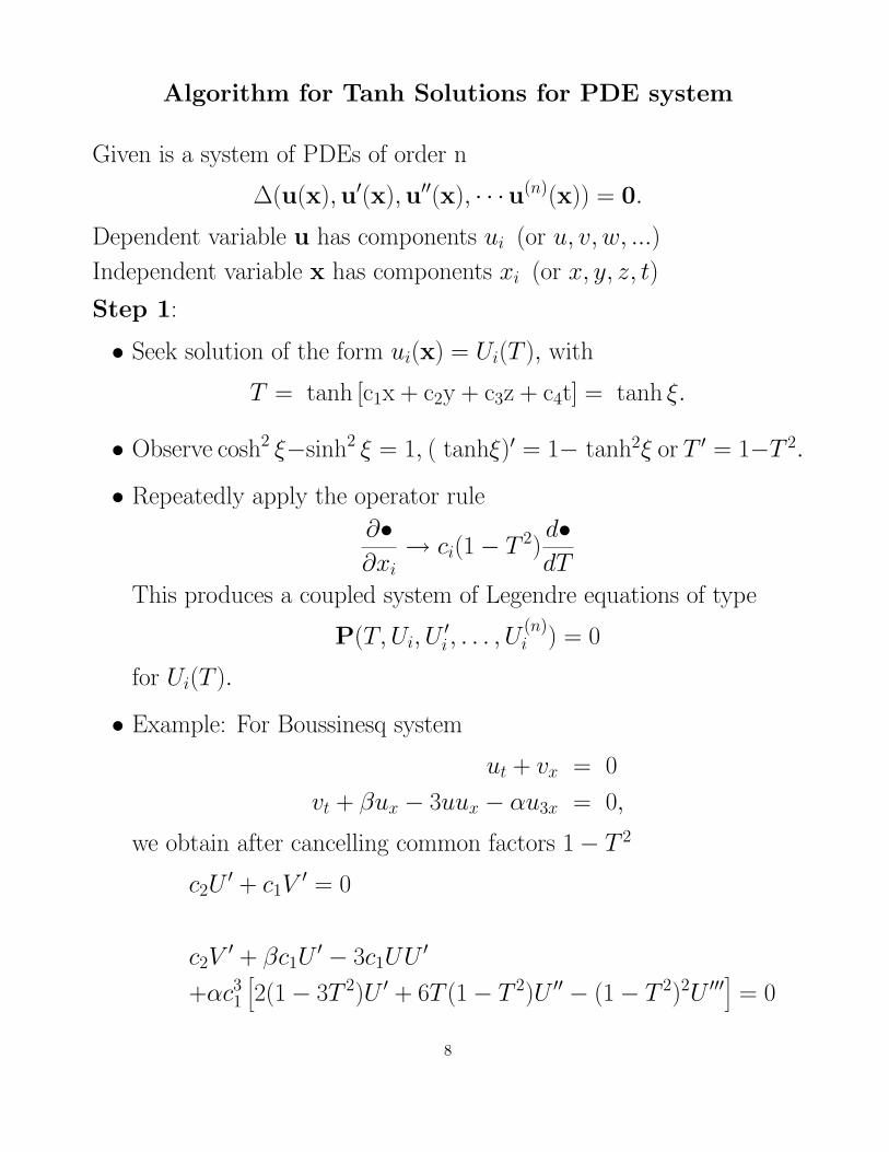
Algorithm for Tanh Solutions for PDE system
Given is a system of PDEs of order n
∆(u(x),u′(x),u′′(x), · · ·u(n)(x)) = 0.
Dependent variable u has components ui (or u, v, w, ...)
Independent variable x has components xi (or x, y, z, t)
Step 1:
• Seek solution of the form ui(x) = Ui(T ), with
T = tanh [c1x + c2y + c3z + c4t] = tanh ξ.
• Observe cosh2 ξ−sinh2 ξ = 1, ( tanhξ)′ = 1− tanh2ξ or T ′ = 1−T 2.
• Repeatedly apply the operator rule
∂•∂xi
→ ci(1− T 2)d•dT
This produces a coupled system of Legendre equations of type
P(T, Ui, U′i , . . . , U
(n)i ) = 0
for Ui(T ).
• Example: For Boussinesq system
ut + vx = 0
vt + βux − 3uux − αu3x = 0,
we obtain after cancelling common factors 1− T 2
c2U′ + c1V
′ = 0
c2V′ + βc1U
′ − 3c1UU ′
+αc31
[2(1− 3T 2)U ′ + 6T (1− T 2)U ′′ − (1− T 2)2U ′′′
]= 0
8

Step 2:
• Seek polynomial solutions
Ui(T ) =Mi∑j=0
aijTj
Balance the highest power terms in T to determine Mi.
• Example: Powers for Boussinesq system
M1 − 1 = M2 − 1, 2M1 − 1 = M1 + 1
gives M1 = M2 = 2.
Hence, U1(T ) = a10 +a11T +a12T2, U2(T ) = a20 +a21T +a22T
2.
Step 3:
• Determine the algebraic system for the unknown coefficients aij by
balancing the coefficients of the various powers of T.
• Example: Boussinesq system
a11 c1 (3a12 + 2α c21) = 0
a12 c1 (a12 + 4α c21) = 0
a21 c1 + a11 c2 = 0
a22 c1 + a12 c2 = 0
βa11 c1 − 3a10 a11 c1 + 2αa11 c31 + a21 c2 = 0
−3a211 c1 + 2β a12 c1 − 6a10 a12 c1 + 16α a12 c3
1 + 2a22 c2 = 0.
9
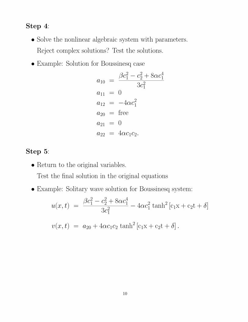
Step 4:
• Solve the nonlinear algebraic system with parameters.
Reject complex solutions? Test the solutions.
• Example: Solution for Boussinesq case
a10 =βc2
1 − c22 + 8αc4
1
3c21
a11 = 0
a12 = −4αc21
a20 = free
a21 = 0
a22 = 4αc1c2.
Step 5:
• Return to the original variables.
Test the final solution in the original equations
• Example: Solitary wave solution for Boussinesq system:
u(x, t) =βc2
1 − c22 + 8αc4
1
3c21
− 4αc21 tanh2 [c1x + c2t + δ]
v(x, t) = a20 + 4αc1c2 tanh2 [c1x + c2t + δ] .
10

Algorithm for Sech Solutions for PDE system
Given is a system of PDEs of order n
∆(u(x),u′(x),u′′(x), · · ·u(n)(x)) = 0.
Dependent variable u has components ui (or u, v, w, ...)
Independent variable x has components xi (or x, y, z, t)
Step 1:
• Seek solution of the form ui(x) = Ui(S), with
S = sech [c1x + c2y + c3z + c4t] = tanh ξ.
• Observe ( sech ξ)′ = − tanh ξ sech ξ or S ′ = −TS = −√
1− S2 S.
Also, cosh2 ξ − sinh2 ξ = 1, hence, T 2 + S2 = 1 and dTdS = −S
T .
• Repeatedly apply the operator rule
∂•∂xi
→ −ci
√1− S2S
d•dS
This produces a coupled system of Legendre type equations of type
P(S, Ui, U′i , . . . , U
(m)i ) +
√1− S2 Q(S, Ui, U
′i , . . . , U
(n)i ) = 0
for Ui(S).
For every equation one must have Pi = 0 or Qi = 0. Only odd
derivatives produce the extra factor√
1− S2.
Conclusion: The total number of derivatives in each term in the
given system should be either even or odd. No mismatch is allowed.
• Example: For the 3D mKdV equation
ut + 6u2ux + uxyz = 0.
11

we obtain after cancelling a common factor −√
1− S2 S
c4U′+6c1U
2U ′+c1c2c3[(1−6S2)U ′+3S(1−2S2)U ′′+S2(1−S2)U ′′′] = 0
Step 2:
• Seek polynomial solutions
Ui(S) =Mi∑j=0
aijSj
Balance the highest power terms in S to determine Mi.
• Example: Powers for the 3D mKdV case
3M1 − 1 = M1 + 1
gives M1 = 1. Hence, U(S) = a10 + a11S.
Step 3:
• Determine the algebraic system for the unknown coefficients aij by
balancing the coefficients of the various powers of S.
• Example: System for 3D mKdV case
a11c1 (a211 − c2 c3) = 0
a11 (6a210 c1 + c1 c2 c3 + c4) = 0
a10 a211 c1 == 0
12
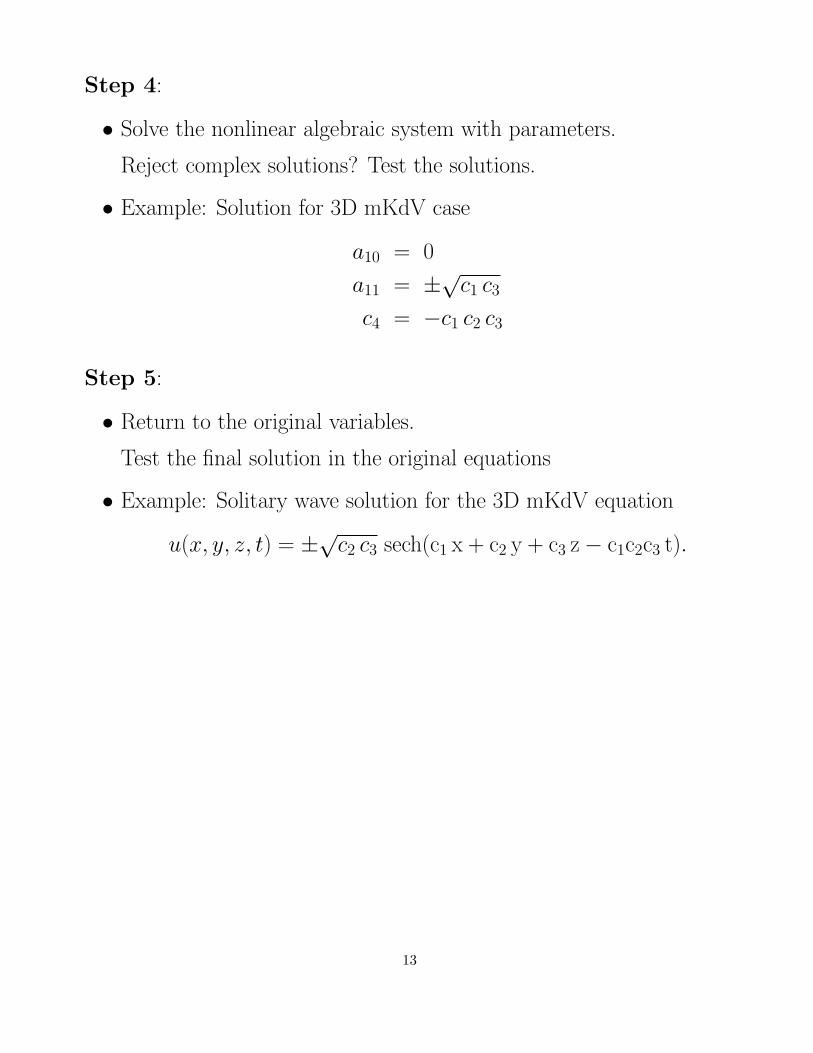
Step 4:
• Solve the nonlinear algebraic system with parameters.
Reject complex solutions? Test the solutions.
• Example: Solution for 3D mKdV case
a10 = 0
a11 = ±√
c1 c3
c4 = −c1 c2 c3
Step 5:
• Return to the original variables.
Test the final solution in the original equations
• Example: Solitary wave solution for the 3D mKdV equation
u(x, y, z, t) = ±√
c2 c3 sech(c1 x + c2 y + c3 z− c1c2c3 t).
13

Extension: Tanh Solutions for DDE system
Given is a system of differential-difference equations (DDEs) of order n
∆(...,un−1,un,un+1, ..., un, ...,u(m)n , ...) = 0.
Dependent variable un has components ui,n (or un, vn, wn, ...)
Independent variable x has components xi (or n, t).
No derivatives on shifted variables are allowed!
Step 1:
• Seek solution of the form ui,n(x) = Ui,n(T (n)), with
T (n) = tanh [c1n + c2t + δ] = tanh ξ.
• Note that the argument T depends on n. Complicates matters.
• Repeatedly apply the operator rule on ui,n
∂•∂t
→ c2(1− T 2)d•dT
This produces a coupled system of Legendre equations of type
P(T, Ui,n, U′i,n, . . .) = 0
for Ui,n(T ).
• Example: Toda lattice
un = (1 + un) (un−1 − 2un + un+1) .
transforms into
c22(1− T 2)
[2TU ′
n − (1− T 2)U ′′n
]+
[1 + c2(1− T 2)U ′
n
][Un−1 − 2Un + Un+1] = 0
14

Step 2:
• Seek polynomial solutions
Ui,n(T (n)) =Mi∑j=0
aijT (n)j
For Un+p, p 6= 0, there is a phase shift:
Ui,n±p (T (n± p) =Mi∑j=0
ai,j [T (n + p)]j =Mi∑j=0
ai,j
T (n)± tanh(pc1)
1± T (n) tanh(pc1)
j
Balance the highest power terms in T (n) to determine Mi.
• Example: Powers for Toda lattice
2M1 − 1 = M1 + 1
gives M1 = 1.
Hence,
Un(T (n)) = a10 + a11T (n)
Un−1(T (n− 1)) = a10 + a11T (n− 1) = a10 + a11T (n)− tanh(c1)
1− T (n) tanh(c1)
Un+1(T (n + 1)) = a10 + a11T (n + 1) = a10 + a11T (n) + tanh(c1)
1 + T (n) tanh(c1).
Step 3:
• Determine the algebraic system for the unknown coefficients aij by
balancing the coefficients of the various powers of T (n).
• Example: Algebraic system for Toda lattice
c22 − tanh2(c1)− a11c2 tanh2(c1) = 0, c2 − a11 = 0
15

Step 4:
• Solve the nonlinear algebraic system with parameters.
Reject complex solutions? Test the solutions.
• Example: Solution of algebraic system for Toda lattice
a10 = free, a11 = c2 = ± sinh(c1)
Step 5:
• Return to the original variables.
Test the final solution in the original equations
• Example: Solitary wave solution for Toda lattice:
un(t) = a0 ± sinh(c1) tanh [c1n± sinh(c1) t + δ] .
16

Example: System of DDEs: Relativistic Toda lattice
un = (1 + αun)(vn − vn−1)
vn = vn(un+1 − un + αvn+1 − αvn−1).
Step 1: Change of variables
un(x, t) = Un(T (n)), vn(x, t) = Vn(T (n)),
with
T (n) = tanh [c1n + c2t + δ] = tanh ξ.
gives
c2(1− T 2)U ′n − (1 + αUn)(Vn − Vn−1) = 0
c2(1− T 2)V ′n − Vn(Un+1 − Un + αVn+1 − αVn−1) = 0.
Step 2: Seek polynomial solutions
Un(T (n)) =M1∑j=0
a1jT (n)j
Vn(T (n)) =M2∑j=0
a2jT (n)j.
Balance the highest power terms in T (n) to determine M1, and M2 :
M1 + 1 = M1 + M2, M2 + 1 = M1 + M2
gives M1 = M2 = 1.
Hence,
Un = a10 + a11T (n), Vn = a20 + a21T (n).
17
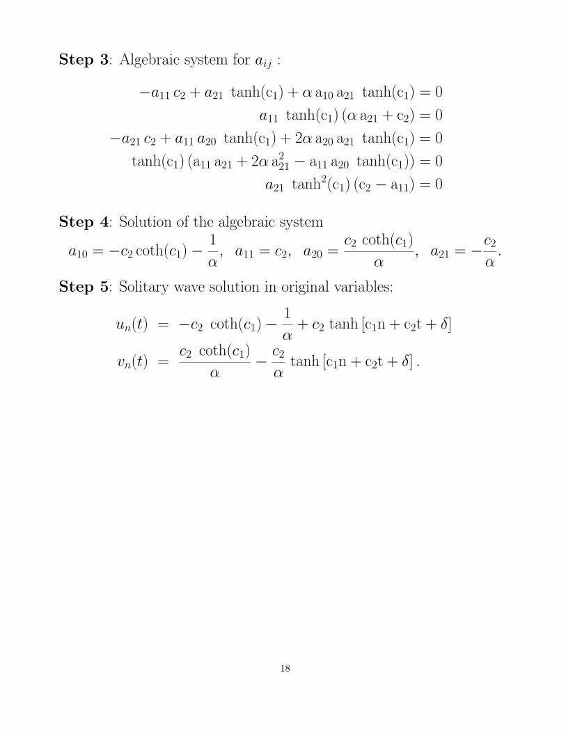
Step 3: Algebraic system for aij :
−a11 c2 + a21 tanh(c1) + α a10 a21 tanh(c1) = 0
a11 tanh(c1) (α a21 + c2) = 0
−a21 c2 + a11 a20 tanh(c1) + 2α a20 a21 tanh(c1) = 0
tanh(c1) (a11 a21 + 2α a221 − a11 a20 tanh(c1)) = 0
a21 tanh2(c1) (c2 − a11) = 0
Step 4: Solution of the algebraic system
a10 = −c2 coth(c1)−1
α, a11 = c2, a20 =
c2 coth(c1)
α, a21 = −c2
α.
Step 5: Solitary wave solution in original variables:
un(t) = −c2 coth(c1)−1
α+ c2 tanh [c1n + c2t + δ]
vn(t) =c2 coth(c1)
α− c2
αtanh [c1n + c2t + δ] .
18

Solving/Analyzing Systems of Algebraic Equations with Parameters
Class of fifth-order evolution equations with parameters:
ut + αγ2u2ux + βγuxu2x + γuu3x + u5x = 0.
Well-Known Special cases
Lax case: α = 310, β = 2, γ = 10. Two solutions:
u(x, t) = 4c21 − 6c2
1 tanh2[c1x− 56c5
1t + δ]
and
u(x, t) = a0 − 2c21 tanh2
[c1x− 2(15a2
0c1 − 40a0c31 + 28c5
1)t + δ]
where a0 is arbitrary.
Sawada-Kotera case: α = 15, β = 1, γ = 5. Two solutions:
u(x, t) = 8c21 − 12c2
1 tanh2[c1x− 16c5
1t + δ]
and
u(x, t) = a0 − 6c21 tanh2
[c1x− (5a2
0c1 − 40a0c31 + 76c5
1)t + δ]
where a0 is arbitrary.
Kaup-Kupershmidt case: α = 15, β = 5
2, γ = 10. Two solutions:
u(x, t) = c21 −
3
2c21 tanh2
[c1x− c5
1t + δ]
and
u(x, t) = 8c21 − 12c2 tanh2
[c1x− 176c5
1t + δ],
no free constants!
Ito case: α = 29, β = 2, γ = 3. One solution:
u(x, t) = 20c21 − 30c2
1 tanh2[c1x− 96c5
1t + δ].
19

What about the General case?
Q1: Can we retrieve the special solutions?
Q2: What are the condition(s) on the parameters α, β, γ for solutions
of tanh-type to exist?
Tanh solutions:
u(x, t) = a0 + a1 tanh [c1x + c2t + δ] + a2 tanh2 [c1x + c2t + δ] .
Nonlinear algebraic system must be analyzed, solved (or reduced!):
a1(αγ2a22 + 6γa2c
21 + 2βγa2c
21 + 24c4
1) = 0
a1(αγ2a21 + 6αγ2a0a2 + 6γa0c
21 − 18γa2c
21 − 12βγa2c
21 − 120c4
1) = 0
αγ2a22 + 12γa2c
21 + 6βγa2c
21 + 360c4
1 = 0
2αγ2a21a2 + 2αγ2a0a
22 + 3γa2
1c21 + βγa2
1c21 + 12γa0a2c
21
−8γa22c
21 − 8βγa2
2c21 − 480a2c
41 = 0
a1(αγ2a20c1 − 2γa0c
31 + 2βγa2c
31 + 16c5
1 + c2) = 0
αγ2a0a21c1 + αγ2a2
0a2c1 − γa21c
31 − βγa2
1c31 − 8γa0a2c
31 + 2βγa2
2c31
+136a2c51 + a2c2 = 0
Unknowns: a0, a1, a2.
Parameters: c1, c2, α, β, γ.
Solve or Reduce should be used on pieces, not on whole system.
20

Strategy to Solve/Reduce Nonlinear Systems
Assumptions:
• All ci 6= 0
• Parameters (α, β, γ, ...) are nonzero. Otherwise the highest powers
Mi may change.
• All aj Mi6= 0. Coefficients of highest power in Ui are present.
• Solve for aij, then ci, then find conditions on parameters.
Strategy followed by hand:
• Solve all linear equations in aij first (cost: branching). Start with
the ones without parameters. Capture constraints in the process.
• Solve linear equations in ci if they are free of aij.
• Solve linear equations in parameters if they free of aij, ci.
• Solve quasi-linear equations for aij, ci, parameters.
• Solve quadratic equations for aij, ci, parameters.
• Eliminate cubic terms for aij, ci, parameters, without solving.
• Show remaining equations, if any.
Alternatives:
• Use (adapted) Grobner Basis Techniques.
• Use combinatorics on coefficients aij = 0 or aij 6= 0.
21

Actual Solution: Two major cases:
CASE 1: a1 = 0, two subcases
Subcase 1-a:
a2 = −3
2a0
c2 = c31(24c2
1 − βγa0)
where a0 is one of the two roots of the quadratic equation:
αγ2a20 − 8γa0c
21 − 4βγa0c
21 + 160c4
1 = 0.
Subcase 1-b: If β = 10α− 1, then
a2 = − 6
αγc21
c2 = − 1
α(α2γ2a2
0c1 − 8αγa0c31 + 12c5
1 + 16αc51)
where a0 is arbitrary.
CASE 2: a1 6= 0, then
α =1
392(39 + 38β + 8β2)
and
a2 = − 168
γ(3 + 2β)c21
provided β is one of the roots of
(104β2 + 886β + 1487)(520β3 + 2158β2 − 1103β − 8871) = 0
22
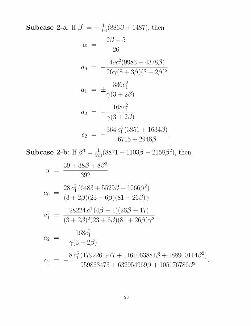
Subcase 2-a: If β2 = − 1104(886β + 1487), then
α = −2β + 5
26
a0 = − 49c21(9983 + 4378β)
26γ(8 + 3β)(3 + 2β)2
a1 = ± 336c21
γ(3 + 2β)
a2 = − 168c21
γ(3 + 2β)
c2 = −364 c51 (3851 + 1634β)
6715 + 2946β.
Subcase 2-b: If β3 = 1520(8871 + 1103β − 2158β2), then
α =39 + 38β + 8β2
392
a0 =28 c2
1 (6483 + 5529β + 1066β2)
(3 + 2β)(23 + 6β)(81 + 26β)γ
a21 =
28224 c41 (4β − 1)(26β − 17)
(3 + 2β)2(23 + 6β)(81 + 26β)γ2
a2 = − 168c21
γ(3 + 2β)
c2 = −8 c51 (1792261977 + 1161063881β + 188900114β2)
959833473 + 632954969β + 105176786β2.
23

Implementation Issues – Mathematica Package
• Demonstration of prototype package
• Demonstration of current package without solver
Future Work
• Look at other types of explicit solutions involving
– hyperbolic functions sinh, cosh, tanh, ...
– other special functions.
– complex exponentials combined with sech or tanh.
• Example: Set of ODEs from quantum field theory
uxx = −u + u3 + auv2
vxx = bv + cv3 + av(u2 − 1).
Try solutions
ui(x, t) =Mi∑j=0
aij tanhj[c1x + c2t + δ] +Ni∑j=0
bij sech2j+1[c1x + c2t + δ].
or
ui(x, t) =Mi∑j=0
(aij + bij sech[c1x + c2t + δ]) tanhj[c1x + c2t + δ].
Obviously, for ODEs c2 = 0.
Solitary wave solutions:
u = ± tanh[
√√√√√√ a2 − c
2(a− c)x + δ]
v = ±√√√√√1− a
a− csech[
√√√√√√ a2 − c
2(a− c)x + δ],
provided b =√
a2−c2(a−c).
24

• Example: Nonlinear Schrodinger equation (focusing/defocusing):
i ut + uxx ± |u|2u = 0.
Bright soliton solution (+ sign):
u(x, t) =k√2
exp[i (c
2x + (k2 − c2
4)t)] sech[k(x− ct− x0)]
Dark soliton solution (− sign):
u(x, t) =1√2
exp[i(Kx− (2k2 + 3K2 − 2Kc +c2
2)t)]
{k tanh[k(x− ct− x0)]− i(K− c
2)}.
• Example: Nonlinear sine-Gordon equation (light cone coordinates):
uxt = sin u.
Setting Φ = ux, Ψ = cos(u)− 1, gives
Φxt − Φ− Φ Ψ = 0
2Ψ + Ψ2 + Φ2t = 0.
Solitary wave solution (kink):
Φ = ux = ± 1√−c
sech[1√−c
(x− ct) + δ],
Ψ = cos(u)− 1 = 1− 2 sech2[1√−c
(x− ct) + δ],
in final form:
u(x, t) = ±4 arctan
exp(1√−c
(x− ct) + δ)
.
25
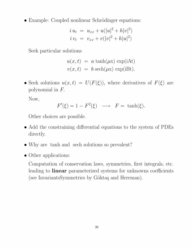
• Example: Coupled nonlinear Schrodinger equations:
i ut = uxx + u(|u|2 + h|v|2)i vt = vxx + v(|v|2 + h|u|2)
Seek particular solutions
u(x, t) = a tanh(µx) exp(iAt)
v(x, t) = b sech(µx) exp(iBt).
• Seek solutions u(x, t) = U(F (ξ)), where derivatives of F (ξ) are
polynomial in F.
Now,
F ′(ξ) = 1− F 2(ξ) −→ F = tanh(ξ).
Other choices are possible.
• Add the constraining differential equations to the system of PDEs
directly.
• Why are tanh and sech solutions so prevalent?
• Other applications:
Computation of conservation laws, symmetries, first integrals, etc.
leading to linear parameterized systems for unknowns coefficients
(see InvariantsSymmetries by Goktas and Hereman).
26