new exact solutions of some nonlinear partial differential ... · pdf filenew exact solutions...
TRANSCRIPT

IJRRAS 18 (2) ● February 2014 www.arpapress.com/Volumes/Vol18Issue2/IJRRAS_18_2_04.pdf
132
NEW EXACT SOLUTIONS OF SOME NONLINEAR PARTIAL
DIFFERENTIAL EQUATIONS VIA THE IMPROVED EXP-FUNCTION
METHOD
M. F. El-Sabbagh, R. Zait and R. M. Abdelazeem
Mathematics Department, Faculty of Science, MiniaUniversity, Egypt.
Corresponding e-mail: [email protected]
ABSTRACT In this paper, we establish new exact solutions of some nonlinear partial differential equations (PDEs) of interest
such as the Kaup–Kupershmidt, the generalized shallow water, the Boussinesq equations via the improved Exp–
function method. Also the method is used to construct periodic and solitary wave solutions for the considered
equations as well.
Keywords: Nonlinear PDEs, Exact solutions, The improved Exp–function method.
1. INTRODUCTION The nonlinear evolution equations (NLEEs) are widely used as models to describe complex physical phenomena in
various field of science, particularly in fluid mechanics, solid state physics, plasma waves and chemical physics.
Nonlinear equations covers also the following subjects: surface wave in compressible fluid, hydro magnetic waves
in cold plasma, acoustic waves in un harmonic crystal, ect. . The wide applicability of these equations is the main
reason for they have attracted so much attention from mathematicians in the last decades. The investigation of the
exact solutions of non linear partial differential equations (PDEs) plays an important role in the study of non-linear
physical phenomena. When we want to understand the physical mechanism of phenomena in nature, described by
non linear PDEs, exact solutions have to be explored. The study of nonlinear PDEs becomes one of the most
important topics in mathematical physics. Recently there are many new methods to obtain exact solutions of
nonlinear PDEs such as sine-cosine function method [1-5], tanh function method [6-8], (𝐺/
𝐺 )-expansion method
[9-13 ], extended Jacobi elliptic function method [14, 15]. He and Wu [16], proposed a straightforward and concise
method, called Exp-function method [17-24], to obtain generalized solitary wave solutions of nonlinear PDEs. Ali
[25] improved this method and obtained new exp-function solutions and periodic solutions as well.
In this paper, we use the improved Exp-function method [25, 26 ] to search for new solitary wave solutions,
compact like solutions and periodic solutions of some nonlinear PDEs, such as the Kaup–Kupershmidt equation
[27-35], the generalized shallow water equation [36, 37], and the Boussinesq equation [38-42].
2. THE IMPROVED EXP-FUNCTION METHOD:
We present the improved Exp-function method [25] in the following steps:
1- Consider the following nonlinear PDE with two independent variables 𝑥, 𝑡 and dependant variable 𝑢:
𝑁(𝑢,𝑢𝑡 ,𝑢𝑥 ,𝑢𝑥𝑥 ,𝑢𝑥𝑡 ,𝑢𝑡𝑡 ,… ) = 0 (1),
where 𝑁 is in general a polynomial function of its argument and the subscripts denote the partial derivatives.
2- We seek a traveling wave solution of Eq. (1) in the form
𝑢 𝑥, 𝑡 = 𝑢 𝜉 , 𝜉 = 𝑘𝑥 + 𝜔𝑡 2 ,
where 𝑘 and 𝜔 are constants to be determined
3- Using the transformation (2), Eq. (1) can be reduced to an ordinary differential equation (ODE):
𝐺 𝑢,𝑢′,𝑢′′,… = 0 3 ,
where 𝐺 is a polynomial of 𝑢 and its derivatives.
4- Through this method, we express the solution of the nonlinear PDE (1) in the form:
IJRRAS 18 (2) ● February 2014 El-Sabbagh & al. ● The Improved Exp-Function Method
133
𝑢 𝜂 = 𝐴𝑗𝑒𝑥𝑝(𝑗𝜉)𝑚
𝑗=0
𝐵𝑖𝑒𝑥𝑝(𝑖𝜉)𝑛𝑖=0
4 ,
where 𝑚 and 𝑛 are positive integers that could be freely chosen.
5- To determine 𝑢 𝑥, 𝑡 explicitly, one may apply the following producer:
(i) Substitute Eq. (4) into Eq. (3), then the lift hand side of Eq. (3) is converted into a polynomial in
𝑒𝑥𝑝(𝜉). Setting all coefficients of 𝑒𝑥𝑝(𝜉) to zero yield a system of algebraic equations for
𝐴0,𝐴1 ,𝐴2,… .𝐴𝑚 , 𝐵0 ,𝐵1 ,𝐵2 ,… .𝐵𝑛 , 𝑘 𝑎𝑛𝑑 𝜔.
(ii) Solve these algebraic equations to obtain A0, A1, A2,… , Am , 𝐵0 ,𝐵1 ,𝐵2 ,… ,𝐵𝑛 , 𝑘 𝑎𝑛𝑑 𝜔.
3. APPLICATIONS In order to illustrate the effectiveness of the above method, examples of mathematical and physical interests are
chosen as follows:
3.1The Kaup–Kupershmidt equation [27-35]
The Kaup–Kupershmidt equation is the nonlinear fifth-order partial differential equation; It is the first equation in a
hierarchy of integrable equations with Lax operator 𝜕3
𝜕𝑥3 + 2𝑢𝜕
𝜕𝑥+
𝜕𝑢
𝜕𝑥. It has properties similar (but not identical) to
those of the better known KdV hierarchy in which the Lax operator has order two.
In the present paper we introduce new exact solutions of the Kaup–Kupershmidt equation via the improved Exp-
function method as follows:
Consider the Kaup–Kupershmidt equation is given as:
𝑢𝑡 = 𝑢𝑥𝑥𝑥𝑥𝑥 − 20𝑢𝑢𝑥𝑥𝑥 − 50𝑢𝑥𝑢𝑥𝑥 + 80𝑢2𝑢𝑥 (5)
Using the transformation:
𝑢 = 𝑢 𝜂 , 𝜂 = 𝑥 − 𝑐𝑡 6 ,
where 𝑐 is a constant to be determined later. Substituting Eq. (6) into Eq. (5) we get
𝑐𝑢′ − 𝑢′′′′′ + 20𝑢𝑢′′′ + 50𝑢′𝑢′′ − 80𝑢2𝑢′ = 0 7 ,
where primes denote derivatives with respect to 𝜂. Now we study the following cases:
𝑪𝒂𝒔𝒆 𝟏: 𝒎 = 𝟐,𝒏 = 𝟐:
According to the improved Exp-function method, the travelling wave solution of Eq. (5) in this case can be written
as:
𝑢 𝑥, 𝑡 = 𝐴0 + 𝐴1𝑒𝑥𝑝(𝜂) + 𝐴2𝑒𝑥𝑝(2𝜂)
𝐵0 + 𝐵1𝑒𝑥𝑝(𝜂) + 𝐵2𝑒𝑥𝑝(2𝜂) (8)
In case 𝐵2 ≠ 0, Eq. (8) can be simplified as:
𝑢 𝑥, 𝑡 = 𝐴0 + 𝐴1𝑒𝑥𝑝(𝜂) + 𝐴2𝑒𝑥𝑝(2𝜂)
𝐵0 + 𝐵1𝑒𝑥𝑝(𝜂) + 𝑒𝑥𝑝(2𝜂) (9)
Substituting Eq. (9) into Eq. (7), and using the Maple, equating to zero the coefficients of all powers of
𝑒𝑥𝑝(𝜂)yields a set of algebraic equations for 𝐴0, 𝐴1, 𝐴2, 𝐵0 ,𝐵1 and c. Solving these system of algebraic equations,
with the aid of Maple, we obtain families of solutions as the following:

IJRRAS 18 (2) ● February 2014 El-Sabbagh & al. ● The Improved Exp-Function Method
134
𝑭𝒂𝒎𝒊𝒍𝒚 𝟏:
𝐵0 = 1,𝐴1 = −5,𝐴0 =1
2, 𝑐 = −11,𝐴2 =
1
2,𝐵1 = 2.
Thus the following solution is
𝑢1 𝑥, 𝑡 =
12− 5𝑒𝑥𝑝(𝑥 + 11𝑡) +
12𝑒𝑥𝑝(2𝑥 + 22𝑡)
1 + 2𝑒𝑥𝑝(𝑥 + 11𝑡) + 𝑒𝑥𝑝(2𝑥 + 22𝑡) (10)
𝑭𝒊𝒈𝒖𝒓𝒆 𝟏. 𝑻𝒓𝒂𝒗𝒆𝒍𝒊𝒏𝒈 𝒘𝒂𝒗𝒆 𝒔𝒐𝒍𝒖𝒕𝒊𝒐𝒏 𝒐𝒇 𝑬𝒒. 𝟓 𝒇𝒐𝒓 𝒔𝒐𝒍𝒖𝒕𝒊𝒐𝒏 𝟏𝟎 .
𝑭𝒂𝒎𝒊𝒍𝒚 𝟐:
𝐵0 = 1,𝐴1 =−5
8,𝐴0 =
1
16, 𝑐 =
−1
16,𝐴2 =
1
16,𝐵1 = 2.
Thus the following solution is
𝑢2 𝑥, 𝑡 =
116
−58𝑒𝑥𝑝(𝑥 +
𝑡16
) +1
16𝑒𝑥𝑝(2𝑥 +
𝑡8
)
1 + 2𝑒𝑥𝑝(𝑥 +𝑡
16) + 𝑒𝑥𝑝(2𝑥 +
𝑡8
) (11)
𝑭𝒊𝒈𝒖𝒓𝒆 𝟐. 𝑻𝒓𝒂𝒗𝒆𝒍𝒊𝒏𝒈 𝒘𝒂𝒗𝒆 𝒔𝒐𝒍𝒖𝒕𝒊𝒐𝒏 𝒐𝒇 𝑬𝒒. 𝟓 𝒇𝒐𝒓 𝒔𝒐𝒍𝒖𝒕𝒊𝒐𝒏 𝟏𝟏 .
𝑪𝒂𝒔𝒆 𝟐: 𝒎 = 𝟑,𝒏 = 𝟑:
According to the improved Exp-function method, the travelling wave solution of Eq. (5) in this case can be written
as:

IJRRAS 18 (2) ● February 2014 El-Sabbagh & al. ● The Improved Exp-Function Method
135
𝑢 𝑥, 𝑡 = 𝐴0 + 𝐴1𝑒𝑥𝑝(𝜂) + 𝐴2𝑒𝑥𝑝(2𝜂) + 𝐴3𝑒𝑥𝑝(3𝜂)
𝐵0 + 𝐵1𝑒𝑥𝑝(𝜂) + 𝐵2𝑒𝑥𝑝(2𝜂) + 𝐵3𝑒𝑥𝑝(3𝜂) (12)
In case 𝐵3 ≠ 0, Eq. (12) can be simplified as:
𝑢 𝑥, 𝑡 = 𝐴0 + 𝐴1𝑒𝑥𝑝(𝜂) + 𝐴2𝑒𝑥𝑝(2𝜂) + 𝐴3𝑒𝑥𝑝(3𝜂)
𝐵0 + 𝐵1𝑒𝑥𝑝(𝜂) + 𝐵2𝑒𝑥𝑝(2𝜂) + 𝑒𝑥𝑝(3𝜂) 13
Substituting Eq. (13) into Eq. (7), and using the Maple, equating to zero the coefficients of all powers of
𝑒𝑥 𝑝 𝜂 yields a set of algebraic equations for 𝐴0, 𝐴1, 𝐴2, 𝐴3, 𝐵0, 𝐵1 ,𝐵2 and c. Solving the system of algebraic
equations given above, with the aid of Maple, we obtain:
𝑭𝒂𝒎𝒊𝒍𝒚 𝟏:
𝐴0 = 0,𝐴1 =1
8𝐵2
2 ,𝐴2 =−5
2𝐵2 ,𝐴3 =
1
2,𝐵0 = 0,𝐵1 =
1
4𝐵2
2 ,𝐵2 = 𝐵2 , 𝑐 = −11.
Thus the following solution is
𝑢5 𝑥, 𝑡 =
14𝐵2
2𝑒𝑥𝑝(𝑥 + 11𝑡) − 5𝐵2𝑒𝑥𝑝(2𝑥 + 22𝑡) + 𝑒𝑥𝑝(3𝑥 + 33𝑡)
12𝐵2
2𝑒𝑥𝑝(𝑥 + 11𝑡) + 2𝐵2𝑒𝑥𝑝(2𝑥 + 22𝑡) + 2𝑒𝑥𝑝(3𝑥 + 33𝑡) (14)
If 𝐵2 = 1, then
𝑢5 𝑥, 𝑡 =
14𝑒𝑥𝑝(𝑥 + 11𝑡) − 5𝑒𝑥𝑝(2𝑥 + 22𝑡) + 𝑒𝑥𝑝(3𝑥 + 33𝑡)
12𝑒𝑥𝑝(𝑥 + 11𝑡) + 2𝑒𝑥𝑝(2𝑥 + 22𝑡) + 2𝑒𝑥𝑝(3𝑥 + 33𝑡)
(15)
𝑭𝒊𝒈𝒖𝒓𝒆 𝟑. 𝑻𝒓𝒂𝒗𝒆𝒍𝒊𝒏𝒈 𝒘𝒂𝒗𝒆 𝒔𝒐𝒍𝒖𝒕𝒊𝒐𝒏 𝒐𝒇 𝑬𝒒. 𝟓 𝒇𝒐𝒓 𝒔𝒐𝒍𝒖𝒕𝒊𝒐𝒏 𝟏𝟓 ,𝑩𝟐 = 𝟏.
𝑭𝒂𝒎𝒊𝒍𝒚 𝟐:
𝐴0 = 0,𝐴1 =1
64𝐵2
2 ,𝐴2 =−5
16𝐵2 ,𝐴3 =
1
16,𝐵0 = 0,𝐵1 =
1
4𝐵2
2 ,𝐵2 = 𝐵2 , 𝑐 = −1
16.
Thus the following solution is
𝑢6 𝑥, 𝑡 =
14𝐵2
2𝑒𝑥𝑝(𝑥 +𝑡
16) − 5𝐵2𝑒𝑥𝑝(2𝑥 +
𝑡8
) + 𝑒𝑥𝑝(3𝑥 +3𝑡16
)
4(𝐵22𝑒𝑥𝑝(𝑥 +
𝑡16
) + 4𝐵2𝑒𝑥𝑝(2𝑥 +𝑡8
) + 4𝑒𝑥𝑝(3𝑥 +3𝑡16
)) (16)
IJRRAS 18 (2) ● February 2014 El-Sabbagh & al. ● The Improved Exp-Function Method
136
If 𝐵2 = 1, then
𝑢6 𝑥, 𝑡 =
14𝑒𝑥𝑝(𝑥 +
𝑡16
) − 5𝑒𝑥𝑝(2𝑥 +𝑡8
) + 𝑒𝑥𝑝(3𝑥 +3𝑡16
)
4(𝑒𝑥 𝑝 𝑥 +𝑡
16 + 4𝑒𝑥 𝑝 2𝑥 +
𝑡8 + 4𝑒𝑥 𝑝 3𝑥 +
3𝑡16
) (17)
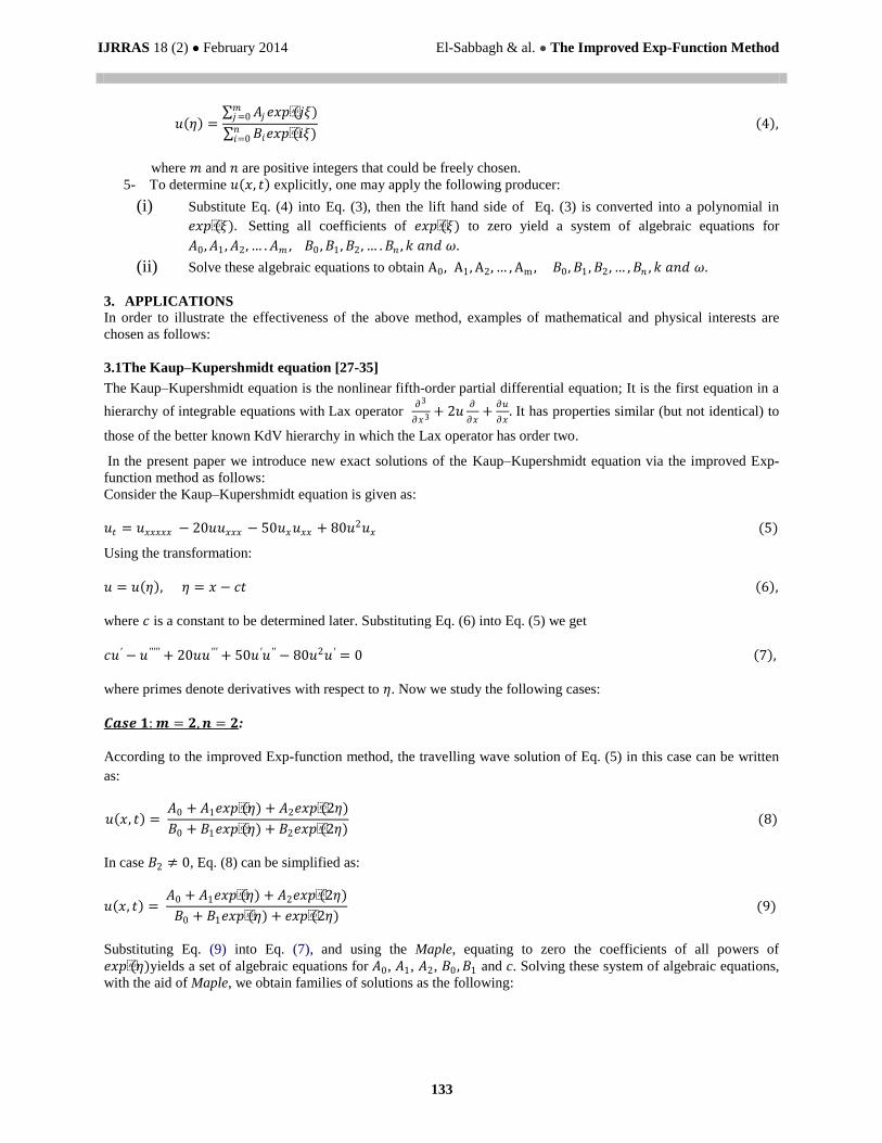
𝑭𝒊𝒈𝒖𝒓𝒆 𝟒. 𝑻𝒓𝒂𝒗𝒆𝒍𝒊𝒏𝒈 𝒘𝒂𝒗𝒆 𝒔𝒐𝒍𝒖𝒕𝒊𝒐𝒏 𝒐𝒇 𝑬𝒒. 𝟓 𝒇𝒐𝒓 𝒔𝒐𝒍𝒖𝒕𝒊𝒐𝒏 𝟏𝟕 ,𝑩𝟐 = 𝟏.
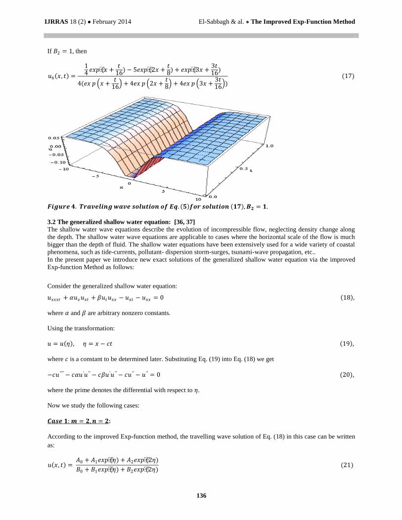
3.2 The generalized shallow water equation: [36, 37]
The shallow water wave equations describe the evolution of incompressible flow, neglecting density change along
the depth. The shallow water wave equations are applicable to cases where the horizontal scale of the flow is much
bigger than the depth of fluid. The shallow water equations have been extensively used for a wide variety of coastal
phenomena, such as tide-currents, pollutant- dispersion storm-surges, tsunami-wave propagation, etc..
In the present paper we introduce new exact solutions of the generalized shallow water equation via the improved
Exp-function Method as follows:
Consider the generalized shallow water equation:
𝑢𝑥𝑥𝑥𝑡 + 𝛼𝑢𝑥𝑢𝑥𝑡 + 𝛽𝑢𝑡𝑢𝑥𝑥 − 𝑢𝑥𝑡 − 𝑢𝑥𝑥 = 0 18 ,
where 𝛼 and 𝛽 are arbitrary nonzero constants.
Using the transformation:
𝑢 = 𝑢 𝜂 , 𝜂 = 𝑥 − 𝑐𝑡 19 ,
where 𝑐 is a constant to be determined later. Substituting Eq. (19) into Eq. (18) we get
−𝑐𝑢′′′′ − 𝑐𝛼𝑢′𝑢′′ − 𝑐𝛽𝑢′𝑢′′ − 𝑐𝑢′′ − 𝑢′′ = 0 (20),
where the prime denotes the differential with respect to 𝜂.
Now we study the following cases:
𝑪𝒂𝒔𝒆 𝟏: 𝒎 = 𝟐,𝒏 = 𝟐:
According to the improved Exp-function method, the travelling wave solution of Eq. (18) in this case can be written
as:
𝑢 𝑥, 𝑡 = 𝐴0 + 𝐴1𝑒𝑥𝑝(𝜂) + 𝐴2𝑒𝑥𝑝(2𝜂)
𝐵0 + 𝐵1𝑒𝑥𝑝(𝜂) + 𝐵2𝑒𝑥𝑝(2𝜂) (21)

IJRRAS 18 (2) ● February 2014 El-Sabbagh & al. ● The Improved Exp-Function Method
137
In case 𝐵2 ≠ 0, Eq.(21) can be simplified as:
𝑢 𝑥, 𝑡 = 𝐴0 + 𝐴1𝑒𝑥𝑝(𝜂) + 𝐴2𝑒𝑥𝑝(2𝜂)
𝐵0 + 𝐵1𝑒𝑥𝑝(𝜂) + 𝑒𝑥𝑝(2𝜂) 22
Substituting Eq. (22) into Eq. (20), and using the Maple, equating to zero the coefficients of all powers of
𝑒𝑥𝑝(𝜂)yields a set of algebraic equations for 𝐴0, 𝐴1, 𝐴2,𝐵0, 𝐵1 and c. Solving the system of algebraic equation
given above, with the aid of Maple, we obtain:
𝐴0 =𝐵0(−24+𝐴2𝛽+𝐴2𝛼)
𝛼+𝛽,𝐴1 = 0,𝐴2 = 𝐴2,𝐵0 = 𝐵0 ,𝐵1 = 0, 𝑐 =
−1
3.
Thus the following solution is
𝑢1 𝑥, 𝑡 =
𝐵0(−24 + 𝐴2𝛽 + 𝐴2𝛼)𝛼 + 𝛽
+ 𝐴2𝑒𝑥𝑝(2𝑥 +2𝑡3
)
𝐵0 + 𝑒𝑥𝑝(2𝑥 +2𝑡3
) (23)
If 𝐴2 = 𝐵0 = 1, 𝛼 = 𝛽 = 2, then
𝑢1 𝑥, 𝑡 =−5 + 𝑒𝑥𝑝(2𝑥 +
2𝑡3
)
1 + 𝑒𝑥𝑝(2𝑥 +2𝑡3
) (24)
𝑭𝒊𝒈𝒖𝒓𝒆 𝟓. 𝑻𝒓𝒂𝒗𝒆𝒍𝒊𝒏𝒈 𝒘𝒂𝒗𝒆 𝒔𝒐𝒍𝒖𝒕𝒊𝒐𝒏 𝒐𝒇 𝑬𝒒. 𝟏𝟖 𝒇𝒐𝒓 𝒔𝒐𝒍𝒖𝒕𝒊𝒐𝒏 𝑬𝒒. 𝟐𝟒 ,𝑨𝟐 = 𝑩𝟎 = 𝟏, 𝜶 = 𝜷 = 𝟐.
𝑪𝒂𝒔𝒆 𝟐: 𝒎 = 𝟑,𝒏 = 𝟑:
According to the improved Exp-function method, the travelling wave solution of Eq. (18) in this case can be written
as:
𝑢 𝑥, 𝑡 = 𝐴0 + 𝐴1𝑒𝑥𝑝(𝜂) + 𝐴2𝑒𝑥𝑝(2𝜂) + 𝐴3𝑒𝑥𝑝(3𝜂)
𝐵0 + 𝐵1𝑒𝑥𝑝(𝜂) + 𝐵2𝑒𝑥𝑝(2𝜂) + 𝐵3𝑒𝑥𝑝(3𝜂) (25)
In case 𝐵3 ≠ 0, Eq.(25) can be simplified as:
𝑢 𝑥, 𝑡 = 𝐴0 + 𝐴1𝑒𝑥𝑝(𝜂) + 𝐴2𝑒𝑥𝑝(2𝜂) + 𝐴3𝑒𝑥𝑝(3𝜂)
𝐵0 + 𝐵1𝑒𝑥𝑝(𝜂) + 𝐵2𝑒𝑥𝑝(2𝜂) + 𝑒𝑥𝑝(3𝜂) 26
Substituting Eq. (26) into Eq. (20), and using the Maple, equating to zero the coefficients of all powers of 𝑒𝑥𝑝(𝜂)
yields a set of algebraic equations for𝐴0, 𝐴1, 𝐴2, 𝐴3, 𝐵0, 𝐵1 ,𝐵2 and c. Solving the system of algebraic equation
given above, with the aid of Maple, we obtain:

IJRRAS 18 (2) ● February 2014 El-Sabbagh & al. ● The Improved Exp-Function Method
138
𝑭𝒂𝒎𝒊𝒍𝒚 𝟏:
𝐴0 = 0,𝐴1 =𝐵1(−24 + 𝐴3𝛽 + 𝐴3𝛼)
𝛼 + 𝛽,𝐴2 = 0,𝐴3 = 𝐴3,𝐵0 = 0,𝐵1 = 𝐵1 ,𝐵2 = 𝐵2 , 𝑐 =
−1
3
Thus the following solution is
𝑢2 𝑥, 𝑡 =
𝐵1(−24 + 𝐴3𝛽 + 𝐴3𝛼)𝛼 + 𝛽
𝑒𝑥𝑝(𝑥 +𝑡3
) + 𝐴3𝑒𝑥𝑝(3𝑥 + 𝑡)
𝐵1𝑒𝑥𝑝(𝑥 +𝑡3
) + 𝑒𝑥𝑝(3𝑥 + 𝑡) (27)
If 𝐵1 = 𝐴3 = 2, 𝛼 = 𝛽 = 1, then
𝑢2 𝑥, 𝑡 =−20𝑒𝑥𝑝(𝑥 +
𝑡3
) + 2𝑒𝑥𝑝(3𝑥 + 𝑡)
2𝑒𝑥𝑝(𝑥 +𝑡3
) + 𝑒𝑥𝑝(3𝑥 + 𝑡) (28)
𝑭𝒊𝒈𝒖𝒓𝒆 𝟔. 𝑻𝒓𝒂𝒗𝒆𝒍𝒊𝒏𝒈 𝒘𝒂𝒗𝒆 𝒔𝒐𝒍𝒖𝒕𝒊𝒐𝒏 𝒐𝒇 𝑬𝒒. 𝟏𝟖 𝒇𝒐𝒓 𝒔𝒐𝒍𝒖𝒕𝒊𝒐𝒏 𝑬𝒒. 𝟐𝟖 ,𝑨𝟑 = 𝑩𝟏 = 𝟐, 𝜶 = 𝜷 = 𝟏.
𝑭𝒂𝒎𝒊𝒍𝒚 𝟐:
𝐴0 =𝐵0(𝐴3𝛽 + 𝐴3𝛼 − 36)
𝛼 + 𝛽,𝐴1 = 0,𝐴2 = 0,𝐴3 = 𝐴3,𝐵0 = 𝐵0 ,𝐵1 = 0,𝐵2 = 0, 𝑐 =
−1
8
Thus the following solution is
𝑢3 𝑥, 𝑡 =
𝐵0(𝐴3𝛽 + 𝐴3𝛼 − 36)𝛼 + 𝛽
+ 𝐴3𝑒𝑥𝑝(3𝑥 +3𝑡8
)
𝐵0 + 𝑒𝑥𝑝(3𝑥 +3𝑡8
) (29)
If 𝐵0 = 𝐴3 = 2, 𝛼 = 𝛽 = 1, then
𝑢3 𝑥, 𝑡 =−32 + 2𝑒𝑥𝑝(3𝑥 +
3𝑡8
)
2 + 𝑒𝑥𝑝(3𝑥 +3𝑡8
) (30)

IJRRAS 18 (2) ● February 2014 El-Sabbagh & al. ● The Improved Exp-Function Method
139
𝑭𝒊𝒈𝒖𝒓𝒆 𝟕. 𝑻𝒓𝒂𝒗𝒆𝒍𝒊𝒏𝒈 𝒘𝒂𝒗𝒆 𝒔𝒐𝒍𝒖𝒕𝒊𝒐𝒏 𝒐𝒇 𝑬𝒒. 𝟏𝟖 𝒇𝒐𝒓 𝒔𝒐𝒍𝒖𝒕𝒊𝒐𝒏 𝑬𝒒. 𝟑𝟎 ,𝑨𝟑 = 𝑩𝟎 = 𝟐,𝜶 = 𝜷 = 𝟏.
3.3 The Boussinesq equation: [38-42]
The Boussinesq-type equations, which include the lowest-order effects of nonlinearity and frequency dispersion as
additions to the simplest non-dispersive linear long wave theory, provide a sound and increasingly well-tested basis
for the simulation of wave propagation in coastal regions. The standard Boussinesq equations for variable water
depth were first derived by Peregrine (1967), who used depth-averaged velocity as a dependent variable.
In the present paper we introduce new exact solutions of the Boussinesq equation via the improved Exp-function
method as follows:
Consider the Boussinesq equation:
𝑢𝑡𝑡 − 𝑢𝑥𝑥 − 𝑢𝑥𝑥𝑥𝑥 − 6(𝑢𝑥)2 − 6𝑢𝑢𝑥𝑥 = 0 (31)
Using the transformation:
𝑢 = 𝑢 𝜂 , 𝜉 = 𝑘𝑥 + 𝜔𝑡 32 ,
where 𝑘,𝜔 are constants to be determined later. Substituting Eq. (32) into Eq. (31) we get
𝜔2𝑢′′ − 𝑘2𝑢′′ − 𝑘4𝑢′′′′ − 6𝑘2(𝑢′)2 − 6𝑘2𝑢𝑢′′ = 0 33 ,
where the prime denotes the differential with respect to 𝜉. Now we study the following cases:
𝑪𝒂𝒔𝒆 𝟏: 𝒎 = 𝟐,𝒏 = 𝟑:
According to the improved Exp-function method, the travelling wave solution of Eq. (31) in this case can be written
as:
𝑢 𝑥, 𝑡 = 𝐴0 + 𝐴1𝑒𝑥𝑝(𝜉) + 𝐴2𝑒𝑥𝑝(2𝜉)
𝐵0 + 𝐵1𝑒𝑥𝑝(𝜉) + 𝐵2𝑒𝑥𝑝(2𝜉) + 𝐵3𝑒𝑥𝑝(3𝜉) (34)
In case 𝐵3 ≠ 0, Eq.(34) can be simplified as:
𝑢 𝑥, 𝑡 = 𝐴0 + 𝐴1𝑒𝑥𝑝(𝜉) + 𝐴2𝑒𝑥𝑝(2𝜉)
𝐵0 + 𝐵1𝑒𝑥𝑝(𝜉) + 𝐵2𝑒𝑥𝑝(2𝜉) + 𝑒𝑥𝑝(3𝜉) 35
Substituting Eq. (35) into Eq. (33), and using the Maple, equating to zero the coefficients of all powers of
𝑒𝑥 𝑝 𝜉 yields a set of algebraic equations for 𝐴0, 𝐴1, 𝐴2, 𝐵0, 𝐵1 ,𝐵2 , 𝑘 𝑎𝑛𝑑 𝜔. Solving the system of algebraic
equation given above, with the aid of Maple, we obtain:

IJRRAS 18 (2) ● February 2014 El-Sabbagh & al. ● The Improved Exp-Function Method
140
𝑭𝒂𝒎𝒊𝒍𝒚 𝟏:
𝐴0 = 0,𝐴1 = 0,𝐴2 = 𝑘2𝐵2 ,𝐵0 = 0,𝐵1 =𝐵2
2
4,𝐵2 = 𝐵2 ,𝜔 = 𝑘 1 + 𝑘2
Thus the following solution is
𝑢1 𝑥, 𝑡 =𝑘2𝐵2𝑒𝑥𝑝(2𝑘𝑥 + 2𝑘𝑡 1 + 𝑘2)
𝐵22
4𝑒𝑥𝑝(𝑘𝑥 + 𝑘𝑡 1 + 𝑘2) + 𝐵2𝑒𝑥𝑝(2𝑘𝑥 + 2𝑘𝑡 1 + 𝑘2) + 𝑒𝑥𝑝(3𝑘𝑥 + 3𝑘𝑡 1 + 𝑘2)
(36)
If 𝑘 = 1, 𝐵2 = 2, then
𝑢1 𝑥, 𝑡 =2𝑒𝑥𝑝(2𝑥 + 2𝑡 2)
𝑒𝑥𝑝(𝑥 + 𝑡 2) + 2𝑒𝑥𝑝(2𝑥 + 2𝑡 2) + 𝑒𝑥𝑝(3𝑥 + 3𝑡 2) (37)
𝑭𝒊𝒈𝒖𝒓𝒆 𝟖. 𝑻𝒓𝒂𝒗𝒆𝒍𝒊𝒏𝒈 𝒘𝒂𝒗𝒆 𝒔𝒐𝒍𝒖𝒕𝒊𝒐𝒏 𝒐𝒇 𝑬𝒒. 𝟑𝟏 𝒇𝒐𝒓 𝒔𝒐𝒍𝒖𝒕𝒊𝒐𝒏 𝑬𝒒. 𝟑𝟕 ,𝑩𝟐 = 𝟐,𝒌 = 𝟏.
𝑭𝒂𝒎𝒊𝒍𝒚 𝟐:
𝐴0 = 0,𝐴1 = 0,𝐴2 = 𝑘2𝐵2 ,𝐵0 = 0,𝐵1 =𝐵2
2
4,𝐵2 = 𝐵2 ,𝜔 = −𝑘 1 + 𝑘2
Thus the following solution is
𝑢2 𝑥, 𝑡 =𝑘2𝐵2𝑒𝑥𝑝(2𝑘𝑥 − 2𝑘𝑡 1 + 𝑘2)
𝐵22
4𝑒𝑥𝑝(𝑘𝑥 − 𝑘𝑡 1 + 𝑘2) + 𝐵2𝑒𝑥𝑝(2𝑘𝑥 − 2𝑘𝑡 1 + 𝑘2) + 𝑒𝑥𝑝(3𝑘𝑥 − 3𝑘𝑡 1 + 𝑘2)
(38)
If 𝐵2 = 2, 𝑘 = 1, then
𝑢2 𝑥, 𝑡 =2𝑒𝑥 𝑝 2𝑥 − 2𝑡 2
𝑒𝑥𝑝(𝑥 − 𝑡 2) + 2𝑒𝑥𝑝(2𝑥 − 2𝑡 2) + 𝑒𝑥𝑝(3𝑥 − 3𝑡 2) (39)

IJRRAS 18 (2) ● February 2014 El-Sabbagh & al. ● The Improved Exp-Function Method
141
𝑭𝒊𝒈𝒖𝒓𝒆 𝟗. 𝑻𝒓𝒂𝒗𝒆𝒍𝒊𝒏𝒈 𝒘𝒂𝒗𝒆 𝒔𝒐𝒍𝒖𝒕𝒊𝒐𝒏 𝒐𝒇 𝑬𝒒. 𝟑𝟏 𝒇𝒐𝒓 𝒔𝒐𝒍𝒖𝒕𝒊𝒐𝒏 𝑬𝒒. 𝟑𝟗 ,𝑩𝟐 = 𝟐,𝒌 = 𝟏.
𝑪𝒂𝒔𝒆 𝟐: 𝒎 = 𝟐,𝒏 = 𝟒:
According to the improved Exp-function method, the travelling wave solution of Eq. (31) in this case can be written
as:
𝑢 𝑥, 𝑡 = 𝐴0 + 𝐴1𝑒𝑥 𝑝 𝜉 + 𝐴2𝑒𝑥 𝑝 2𝜉
𝐵0 + 𝐵1𝑒𝑥 𝑝 𝜉 + 𝐵2𝑒𝑥 𝑝 2𝜉 + 𝐵3𝑒𝑥 𝑝 3𝜉 + 𝐵4𝑒𝑥 𝑝 4𝜉 (40)
In case 𝐵4 ≠ 0, Eq.(40) can be simplified as:
𝑢 𝑥, 𝑡 = 𝐴0 + 𝐴1𝑒𝑥 𝑝 𝜉 + 𝐴2𝑒𝑥 𝑝 2𝜉
𝐵0 + 𝐵1𝑒𝑥 𝑝 𝜉 + 𝐵2𝑒𝑥 𝑝 2𝜉 + 𝐵3𝑒𝑥 𝑝 3𝜉 + 𝑒𝑥 𝑝 4𝜉 41
Substituting Eq. (41) into Eq. (33), and using the Maple, equating to zero the coefficients of all powers of
𝑒𝑥 𝑝 𝜉 yields a set of algebraic equations for 𝐴0, 𝐴1, 𝐴2, 𝐵0 , 𝐵1 ,𝐵2 ,𝐵3 , 𝑘 and 𝜔. Solving the system of algebraic
equation given above, with the aid of Maple, we obtain:
𝑭𝒂𝒎𝒊𝒍𝒚 𝟏:
𝐴0 = 0,𝐴1 = 0,𝐴2 = 𝐴2,𝐵0 =𝐴2
2
64𝑘4,𝐵1 = 0,𝐵2 =
𝐴2
4𝑘2,𝐵3 = 𝐵3 ,𝜔 = 𝑘 1 + 4𝑘2
Thus the following solution is
𝑢3 𝑥, 𝑡 =𝐴2𝑒𝑥𝑝(2𝑘𝑥 + 2𝑘𝑡 1 + 4𝑘2)
𝐴22
64𝑘4 +𝐴2
4𝑘2 𝑒𝑥𝑝(2𝑘𝑥 + 2𝑘𝑡 1 + 4𝑘2) + 𝑒𝑥𝑝(4𝑘𝑥 + 4𝑘𝑡 1 + 4𝑘2)
(42)
If 𝐴2 = 2, 𝑘 = 1, then
𝑢3 𝑥, 𝑡 =2𝑒𝑥𝑝(2𝑥 + 2𝑡 5)
116
+12𝑒𝑥𝑝(2𝑥 + 2𝑡 5) + 𝑒𝑥𝑝(4𝑥 + 4𝑡 5)
(43)
IJRRAS 18 (2) ● February 2014 El-Sabbagh & al. ● The Improved Exp-Function Method
142
𝑭𝒊𝒈𝒖𝒓𝒆 𝟏𝟎. 𝑻𝒓𝒂𝒗𝒆𝒍𝒊𝒏𝒈 𝒘𝒂𝒗𝒆 𝒔𝒐𝒍𝒖𝒕𝒊𝒐𝒏 𝒐𝒇 𝑬𝒒. 𝟑𝟏 𝒇𝒐𝒓 𝒔𝒐𝒍𝒖𝒕𝒊𝒐𝒏 𝑬𝒒. 𝟒𝟑 ,𝑨𝟐 = 𝟐,𝒌 = 𝟏.
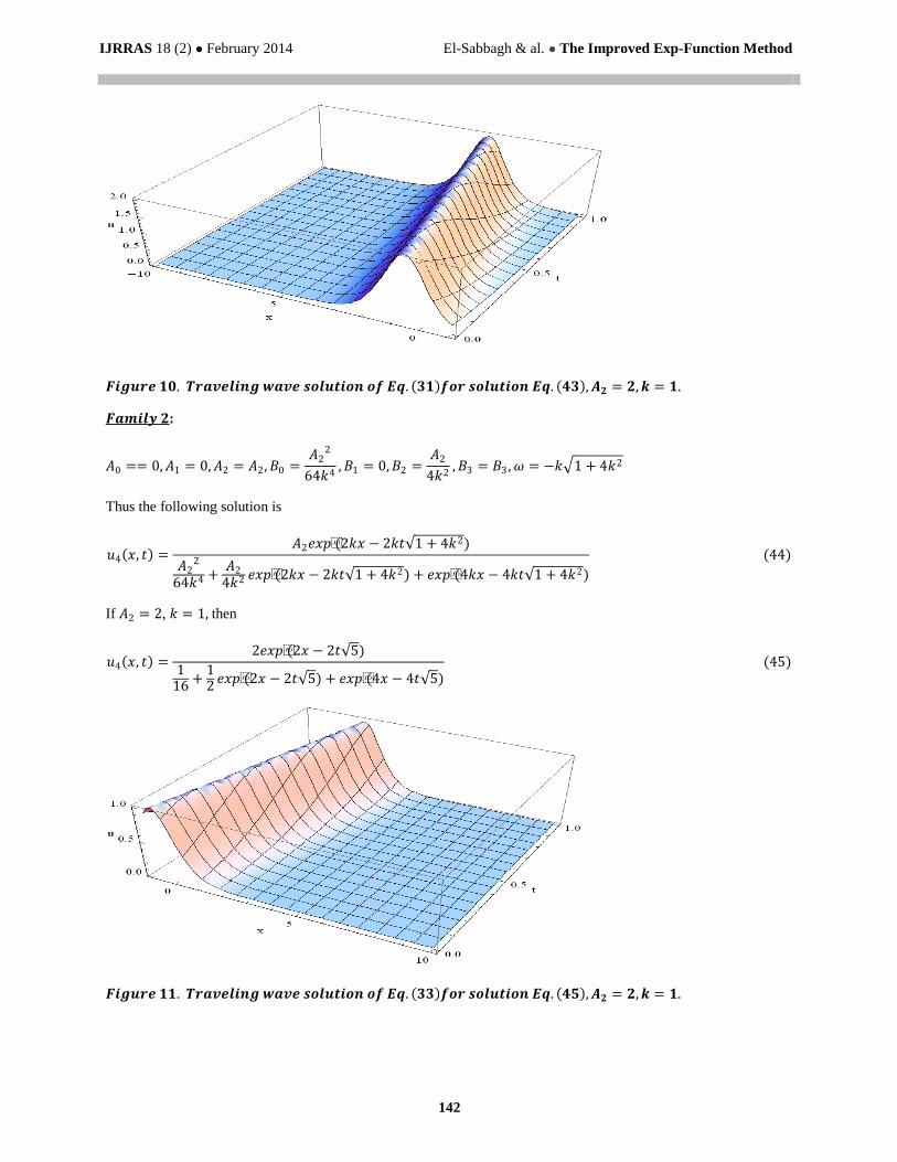
𝑭𝒂𝒎𝒊𝒍𝒚 𝟐:
𝐴0 == 0,𝐴1 = 0,𝐴2 = 𝐴2,𝐵0 =𝐴2
2
64𝑘4,𝐵1 = 0,𝐵2 =
𝐴2
4𝑘2,𝐵3 = 𝐵3 ,𝜔 = −𝑘 1 + 4𝑘2
Thus the following solution is
𝑢4 𝑥, 𝑡 =𝐴2𝑒𝑥𝑝(2𝑘𝑥 − 2𝑘𝑡 1 + 4𝑘2)
𝐴22
64𝑘4 +𝐴2
4𝑘2 𝑒𝑥𝑝(2𝑘𝑥 − 2𝑘𝑡 1 + 4𝑘2) + 𝑒𝑥𝑝(4𝑘𝑥 − 4𝑘𝑡 1 + 4𝑘2)
(44)
If 𝐴2 = 2, 𝑘 = 1, then
𝑢4 𝑥, 𝑡 =2𝑒𝑥𝑝(2𝑥 − 2𝑡 5)
116
+12𝑒𝑥𝑝(2𝑥 − 2𝑡 5) + 𝑒𝑥𝑝(4𝑥 − 4𝑡 5)
(45)
𝑭𝒊𝒈𝒖𝒓𝒆 𝟏𝟏. 𝑻𝒓𝒂𝒗𝒆𝒍𝒊𝒏𝒈 𝒘𝒂𝒗𝒆 𝒔𝒐𝒍𝒖𝒕𝒊𝒐𝒏 𝒐𝒇 𝑬𝒒. 𝟑𝟑 𝒇𝒐𝒓 𝒔𝒐𝒍𝒖𝒕𝒊𝒐𝒏 𝑬𝒒. 𝟒𝟓 ,𝑨𝟐 = 𝟐,𝒌 = 𝟏.

IJRRAS 18 (2) ● February 2014 El-Sabbagh & al. ● The Improved Exp-Function Method
143
4. CONCULSION
In this paper, the improved Exp-function method has been successfully applied to obtain new solutions of three
nonlinear partial differential equations. Thus, the improved Exp-function method can be extended to solve the
problems of nonlinear partial differential equations which arising in the theory of solitons and other areas.
5. REFERENCES
[1]. M.T. Alquran, Solitons And Periodic Solutions To Nonlinear Partial Differential Equations By The Sine-
Cosine Method, Appl. Math. Inf. Sci. 6, No. 1, pp. 85-88, 2012.
[2]. S. A. Mohammad-Abadi, Analytic Solutions Of The Kadomtsev-Petviashvili Equation With Power Law
Nonlinearity Using The Sine-Cosine Method, American Journal of Computational and Applied Mathematics,
Vol. 1,No. 2, pp. 63-66, 2011.
[3]. A. J. M. Jawad, The Sine-Cosine Function Method For The Exact Solutions Of Nonlinear Partial Differential
Equations, IJRRAS, Vol. 13, No. 1, 2012.
[4]. M. Hosseini, H. Abdollahzadeh, M.Abdollahzadeh, Exact Travelling Solutions For The Sixth-Order
Boussinesq Equation, The Journal of Mathematics and Computer Science Vol. 2, No.2, pp. 376-387, 2011.
[5]. S. Arbabi, M. Najafi, M. Najafi, New Periodic And Soliton Solutions Of (2 + 1)-Dimensional Soliton
Equation, Journal of Advanced Computer Science and Technology, Vol.1, No. 4, pp. 232-239, 2012.
[6]. A. J. M. Jawad, M. D. Petkovic and A. Biswas, Soliton Solutions To A few Coupled Nonlinear Wave
Equations By Tanh Method, IJST, 37A2,pp. 109-115, 2013.
[7]. A. J. Muhammad-Jawad, Tanh Method For Solutions Of Non-linear Evolution Equations, Journal of Basrah
Researches (Sciences), Vol. 37. No. 4, 2011.
[8]. W. Malfliet, W. Hereman, The Tanh Method: 1. Exact Solutions Of Nonlinear Evolution And Wave
Equations, Physica Scripta. Vol. 54, pp. 563-568, (1996).
[9]. J. F.Alzaidy, The (G'/G) - Expansion Method For Finding Traveling Wave Solutions Of Some Nonlinear
Pdes In Mathematical Physics, IJMER, Vol.3, Issue.1, pp. 369-376, 2013.
[10]. G. Khaled A, AGeneralized (G´/G)-Expansion Method To Find The Traveling Wave Solutions Of Nonlinear
Evolution Equations, J. Part. Diff. Eq., Vol. 24, No. 1, pp.55-69, 2011.
[11]. J. Manafianheris, Exact Solutions Of The BBM And MBBM Equations By The Generalized (G'/G )-
Expansion Method Equations, International Journal of Genetic Engineering, Vol. 2, No. 3, pp. 28-32, 2012.
[12]. Y. Qiu and B. Tian, Generalized G'/G-Expansion Method And Its Applications, International Mathematical
Forum, Vol. 6, No. 3, pp. 147 – 157, 2011.
[13]. R. K. Gupta, S. Kumar, and B. Lal, New Exact Travelling Wave Solutions Of Generalized Sinh-Gordon And
(2 + 1)-Dimensional ZK-BBM Equations, Maejo Int. J. Sci. Technol.,Vol. 6, pp. 344-355, 2012.
[14]. A. S. Alofi, Extended Jacobi Elliptic Function Expansion Method For Nonlinear Benjamin-Bona-Mahony
Equations, International Mathematical Forum, Vol. 7, No.53, pp. 2639 – 2649, 2012.
[15]. B. Hong, D. Lu2, and F. Sun, The Extended Jacobi Elliptic Functions Expansion Method And New Exact
Solutions For The Zakharov Equations, World Journal of Modelling and Simulation, Vol. 5, No. 3, pp. 216-
224, 2009.
[16]. J. H. He and X. H. Wu, Exp-function Method For Nonlinear Wave Equations, Chaos, Solitons & Fractals,
Vol. 30, pp.700-708, 2006.
[17]. A. Ebaid, Exact Solitary Wave Solutions For Some Nonlinear Evolution Equations Via Exp-function Method,
Physics Letters A 365, pp. 213–219, 2007.
[18]. A. Boz, A. Bekir, Application Of Exp-function Method For (2 + 1)-Dimensional Nonlinear Evolution
Equations, Chaos, Solitons and Fractals, Vol. 40, issue 1, pp. 458-465, 2009.
[19]. A. Boz, A. Bekir, Application Of Exp-function Method For (3 + 1)-Dimensional Nonlinear Evolution
Equations, Computers and Mathematics with Applications, Vol. 56, pp.1451–1456, 2008.
[20]. Z.Sheng, Application Of Exp-function Method To High-dimensional Nonlinear Evolution Equation, Chaos,
Solitons and Fractals, Vol. 38, pp. 270–276, 2008.
[21]. Z. Sheng, Exp-function Method Exactly Solving A KdV Equation With Forcing Term, Applied Mathematics
and Computation, Vol. 197, pp. 128–134, 2008.
[22]. Yusufo˘glu. E, New Solitonary Solutions For Modified Forms Of DP And CH Equations Using Exp-function
Method, Chaos, Solitons and Fractals xxx (2007) xxx–xxx.
[23]. Yusufo˘glu. E, New Solitonary Solutions For The MBBM Equations Using Exp-function Method, Physics
Letters A 372, pp. 442–446, 2008.
[24]. E. Misirli, Y. Gurefe, EXP-Function Method For Solving Nonlinear Evolution Equations, Mathematical and
Computational Applications, Vol. 16, No. 1, pp. 258-266, 2011.

IJRRAS 18 (2) ● February 2014 El-Sabbagh & al. ● The Improved Exp-Function Method
144
[25]. A.T.Ali, A note On The Exp-function Method And Its Application To Nonlinear Equations, Phys. Scr., Vol.
79, Issue 2, id. 025006, 2009.
[26]. M. F. El-Sabbagh , M. M. Hassan and E Hamed , New Solutions For Some Non-linear Evolution Equations
Using Improved Exp-function Method, El-Minia Science Bulletin,Vol. 21, pp. 1-25, 2010.
[27]. A. Khajeh, A. Yousefi-Koma, V. Maryam and M.M. Kabir, Exact Travelling Wave Solutions For Some
Nonlinear Equations Arising In Biology And Engineering, World Applied Sciences Journal, Vol. 9, No. 12,
pp. 1433-1442, 2010.
[28]. F. Dahe, L. Kezan, On Exact Traveling Wave Solutions For (1 + 1) Dimensional Kaup Kupershmidt
Equation, Applied Mathematics, Vol. 2 , pp. 752-756 , 2011.
[29]. F. Qinghua, New Analytical Solutions For (3+1) Dimensional Kaup-Kupershmidt Equation, International
Conference on Computer Technology and Science, Vol. 47, No. 59, 2012.
[30]. F. XIE and X.GAO, A Computational Approach To The New Type Solutions Of Whitham Broer Kaup
Equation In Shallow Water, Commun. Theor. Phys. (Beijing, China), Vol. 41, No. 2, pp. 179–182, 2004.
[31]. H. L¨U and X. LIU, Exact Solutions To (2+1)-Dimensional Kaup Kupershmidt Equation, Commun. Theor.
Phys.(Beijing, China), Vol. 52, No. 5, pp. 795–800, 2009.
[32]. H. Salas Alvaro, Exact Solutions To Kaup-Kupershmidt Equation By Projective Riccati Equations Method,
International Mathematical Forum, Vol. 7, No. 8, pp. 391 – 396, 2012.
[33]. L. Jibin and Z. Qiao, Explicit Soliton Solutions Of The Kaup-Kupershmidt Equation Through The Dynamical
System Approach, Journal of Applied Analysis and Computation, Vol. 1, No. 2, pp. 243–250, 2011.
[34]. P. Saucez , A.Vande Wouwer, W.E. Schiesserc, P.Zegeling, Method Of Lines Study Of Nonlinear Dispersive
Waves, Journal of Computational and Applied Mathematics, Vol. 168, pp. 413–423, 2004.
[35]. V. D. Maria and Nikolai A. Kudryashov, Point Vortices And Polynomials Of The Sawada Kotera And Kaup
Kupershmidt Equations, Regular and Chaotic Dynamics, Vol. 16, No. 6, pp. 562–576, 2011.
[36]. S. A. El-Wakil, M.A. Abdou, A. Hendi, New Periodic Wave Solutions Via Exp-function Method, Physics
Letters A 372, pp. 830 840, 2008.
[37]. V. Anjali, J. Ram and K. Jitender, Traveling Wave Solutions For Shallow Water Wave Equation B𝑦 𝐺\
𝐺 -
Expansion Method, International Journal Of Mathematical Sciences, Vol. 7, No. 1, 2013.
[38]. A. R. Seadawy, The Solutions Of The Boussinesq And Generalized Fifth-Order KdV Equations By Using
The Direct Algebraic Method, Applied Mathematical Sciences, Vol. 6, No. 82, pp.4081 – 4090, 2012.
[39]. E. Yusufo˘glu, New Solitonary Solutions For The MBBM Equations Using Exp-function Method, Physics
Letters A 372, pp. 442–446, 2008.
[40]. L.V. Bogdanov, V.E. Zakharov, The Boussinesq Equation Revisited, Physica D, Vol. 165, pp. 137–162,
2002.
[41]. L.Wei, Z. Jinhua, Z. Yunmei , Exact Solutions For A family Of Boussinesq Equation With Nonlinear
Dispersion, International Journal of Pure and Applied Mathematics, Vol. 76, No. 1, pp. 49-68, 2012.
[42]. M. A. Abdou, A. A. Soliman, S.T. El-Basyony, New Application Of Exp-function Method For Improved
Boussinesq Equation, Physics Letters A 369, pp. 469–475, 2007.