ABSTRACT

MOORE, AMBER DAWN. Modeling erosion on construction sites (Under the direction of

Richard A. McLaughlin and Keith Cassel.)

Our first objective was to develop suitable construction site parameters for the validated

WEPP erosion prediction model. Predicted values were correlated with field observations for

runoff and sediment yield. Runoff volumes and sediment yields similar to those measured on

an active construction site were achieved by removing the A horizon from the soil input

parameter and applying a landcover parameter with no ground cover and minimal roughness.

Increasing critical shear stress to 384 Pa (as recommended by an erosion mat manufacturer)

efficiently predicted runoff volume (E = 0.66) and sediment yield (E = 0.57) when compared

to a construction site stabilized with straw, tar and erosion blankets.

Our second and third objectives were to use to evaluate state-approved sediment traps

and riparian buffers with WEPP and GeoWEPP, and to create erosion and sediment control

scenarios that would achieve the NC water quality standard of 50 Nephlometric Turbidity

Units. Two sediment traps on an actual school construction site were modeled with WEPP,

and a 15.2 m width forest buffer on a planned golf course site was modeled with GeoWEPP.

WEPP predicted average trapping efficiencies of sediment traps A and B to meet the NC

standard of 70 % trapping efficiency. WEPP predicted runoff from sediment trap B met the

turbidity standard for 11 % of the modeled storm events. GeoWEPP predicted that the

riparian buffers would not meet the turbidity standard for any of the modeled storm events.

The existing sediment controls were adjusted to meet water quality standards by increasing

sediment trap size, replacing free-draining traps rock outlets with standing pools behind

culvert outlets, extending the riparian buffer, and adding vegetation to highly erosive areas

iii

determined by GeoWEPP. Turbidity standards were met on watershed A by removing the

outlet from the second sediment trap and increasing the trap area 6-fold. WEPP and

GeoWEPP are useful for modeling construction sites and for designing erosion control

scenarios, although the new parameters and the GeoWEPP model will need to be validated

on other construction sites to improve confidence in the model output.

Modeling Erosion on Construction Sites

by

Amber Moore

A dissertation submitted to the Graduate Faculty of

North Carolina State University

In partial fulfillment of the

Requirements for the degree of

Doctor of Philosophy

In

Soil Science

Raleigh, NC

2004

Approved by:

Rich McLaughlin, Chair of Advisory Committee

Keith Cassel, Co-chair

Helena Mitasova Greg Jennings

ii

BIOGRAPHY

Amber was raised in Soddy-Daisy, Tennessee by her parents, Shirley and Roger, with

her siblings, Eric and Kala. Growing up she enjoyed activities such as playing soccer,

performing the clarinet, and spending summers riding horses at Girl Scout camp. After high

school she moved to Alabama, where she completed a B.S. degree in Environmental Science

at Auburn University. Wanting to combine her interests in working with children and

protecting the environment, Amber moved to Trinity, Texas to work at the Outdoor

Education Center, a state-funded program for fifth grade children from Houston, Texas.

While in Texas, Amber was inspired to return to college to strengthen her environmental

science background. Two years later she moved to Raleigh, N.C. to pursue a M.S. in Soil

Science at North Carolina State University under Rob Mikkelsen, where her research focused

on nitrogen availability of swine lagoon. Shifting her focus from soil fertility to soil physics,

she collaborated with Rich McLaughlin and Helena Mitasova for her Ph.D., focusing her

research on erosion prediction models and best management practices on construction sites.

Upon the completion of her Ph.D. degree, she plans to decompress from five consecutive

years of graduate school, eventually pursuing a postdoctoral research position in the field of

soil erosion. When Amber finds a moment of free time, she practices yoga in her living

room, goes jogging around town, and pretends to pedal on the back of Chloe's tandem

bicycle. She is also fond of trying new vegetarian recipes, watching independent films,

encouraging Chloe's rottweiler to chase the cat, and tending to her tiny garden when the

mood hits her.

iii

ACKNOWLEDGMENTS

There are several people that I would like to recognize for their support toward the

completion of my doctoral dissertation. I would like to thank my advisor Rich McLaughlin

and committee member Helena Mitasova for helping me pick up the pieces of a project that

completely fell apart, and for taking such a personal interest in the progress of my research. I

would also like to thank committee members Greg Jennings and Keith Cassel, who continue

to offer support no matter how many new fancy positions they decide to accept. I would like

to thank Dan Line, who loaned me the data I needed to answer so many of the questions we

were asking. I would like to thank Jamie Stansell, Sara Hayes, Freddie Aldridge, Wesley

Childres, Tabitha Brown, and Dawn Deojay, for retrieving and analyzing an endless amount

of dirty water. I would like to thank Rob Austin for pulling me out of more than one GIS-

related pickle. Finally, I would like to thank Chloe Palenchar, for, again, spending nights in

the lab while I wrote, and for editing my chapters. Thank you.

iv

TABLE OF CONTENTS

LIST OF FIGURES ................................................................................................................................VII

LIST OF TABLES ................................................................................................................................... XI

LIST OF ABBREVIATIONS .............................................................................................................. XIII

CHAPTER 1: INTRODUCTION TO SEDIMENT POLLUTION FROM CONSTRUCTION SITES

AND EROSION PREDICTION MODELING ..................................................................................................1

INTRODUCTION .........................................................................................................................................1

NEGATIVE IMPACTS OF SEDIMENT POLLUTION.........................................................................................1

AQUATIC LIFE...........................................................................................................................................2

ECONOMICS ..............................................................................................................................................3

AESTHETICS..............................................................................................................................................4

TARGET AREAS FOR CONTROLLING EROSION...........................................................................................5

Agriculture ..........................................................................................................................................5

Construction sites ................................................................................................................................5

Regulations..........................................................................................................................................6

USING MODELS TO OPTIMIZE BMP EFFICIENCY........................................................................................8

EROSION PREDICTION MODELING.............................................................................................................9

OBJECTIVES ............................................................................................................................................12

REFERENCES ...........................................................................................................................................12

CHAPTER 2: ADAPTING WEPP MODEL PARAMETERS FOR EROSION PREDICTION ON

CONSTRUCTION SITES .................................................................................................................................18

INTRODUCTION .......................................................................................................................................18

METHODS AND MATERIALS ....................................................................................................................21

Site Description .................................................................................................................................21

v

Field Sampling ..................................................................................................................................25

Watershed monitoring .................................................................................................................................. 25

Sediment yield estimation............................................................................................................................. 26

Model Description.............................................................................................................................28

Model Inputs......................................................................................................................................29

Calibration ........................................................................................................................................30

Calibration of soil inputs .............................................................................................................................. 31

Calibration of landcover inputs..................................................................................................................... 32

RESULTS AND DISCUSSION .....................................................................................................................34

Calibration ........................................................................................................................................34

Pre-construction phase – Centennial A & C watersheds............................................................................... 35

During construction – Carpenter watershed.................................................................................................. 40

Temporary Stabilization – Carpenter watershed........................................................................................... 46

Parameter Recommendations............................................................................................................52

CONCLUSION...........................................................................................................................................53

REFERENCES ...........................................................................................................................................54

APPENDIX ...............................................................................................................................................59

CHAPTER 3: APPLYING PROCESS-BASED MODELS FOR EROSION AND SEDIMENT

CONTROL DESIGN..........................................................................................................................................69

INTRODUCTION .......................................................................................................................................70

METHODS AND MATERIALS ....................................................................................................................72

Site description ..................................................................................................................................72

Model Descriptions ...........................................................................................................................75

WEPP ........................................................................................................................................................... 75

GeoWEPP..................................................................................................................................................... 77

Model Inputs......................................................................................................................................78

WEPP ........................................................................................................................................................... 78

vi

GeoWEPP..................................................................................................................................................... 81

Methods for Optimizing BMPs ..........................................................................................................81

RESULTS AND DISCUSSION .....................................................................................................................85

Efficiency of planned BMPs ..............................................................................................................85

WEPP Impoundments................................................................................................................................... 85

GeoWEPP Vegetation .................................................................................................................................. 87

Using models to meet NC water quality standard .............................................................................89

WEPP Impoundments................................................................................................................................... 89

GeoWEPP Vegetation .................................................................................................................................. 93

CONCLUSION.........................................................................................................................................103

REFERENCES .........................................................................................................................................103

APPENDIX .............................................................................................................................................108

vii

LIST OF FIGURES

Figure 2-1. Landcoverage maps of Centennial watershed A (above) and C (below), located on the North Carolina State University Centennial Campus Middle School in Raleigh, North Carolina. Watersheds were delineated in GeoWEPP with TOPAZ software. . 22

Figure 2-2. . Landcoverage maps of the Carpenter watershed during construction (above) and during site stabilization (below), located on the Carpenter Village Residential Community in Carpenter, North Carolina. Watersheds were delineated in GeoWEPP with TOPAZ software. Watershed boundaries before and after construction were altered as a result of clearing and grading changes made at the site........................... 23

Figure 2-3. Sediment load (as suspended solids) and runoff volume exiting the sediment trap at the Carpenter watershed in Carpenter, North Carolina from December 10, 1997 to April 25, 2000. ............................................................................................................ 26

Figure 2-4. Relationship between TSS and turbidity in runoff samples collected from watershed outlets from the Centennial site. ................................................................ 27

Figure 2-5. Observed and WEPP predicted (a) runoff volumes and (b) sediment yields for Centennial watersheds A (area = 9.3 ha) & C (area = 11.8 ha), applying the Disturbed/forest landcover parameter for the pre-construction phase. ....................... 38

Figure 2-6. GeoWEPP generated annual soil loss map for Centennial watershed A for the pre-construction phase. (DEM elevations exaggerated 5X to clearly illustrate topographical characteristics). .................................................................................... 39

Figure 2-7. GeoWEPP generated annual soil loss map for Centennial watershed C for the pre-construction phase. (DEM elevations exaggerated 5X to clearly illustrate topographical characteristics). .................................................................................... 40

Figure 2-8. Observed and WEPP predicted runoff volumes for Carpenter during the construction phase, applying WEPP clay loam Cutslope soil parameter. .................. 43

Figure 2-9. Observed and WEPP predicted runoff volumes for Carpenter during the construction phase, applying WEPP individual soil series soil parameter with the A horizon. ....................................................................................................................... 43

Figure 2-10. Observed and WEPP predicted runoff volumes for Carpenter watershed , applying WEPP individual soil series soil parameter without the A horizon along with the “Baresoil” landcover. ............................................................................................ 44

viii

Figure 2-11. Observed and WEPP predicted sediment yields for Carpenter watershed , applying WEPP individual soil series soil parameter without the A horizon along with the “Baresoil” landcover. ............................................................................................ 45

Figure 2-12. GeoWEPP generated annual soil loss map for Carpenter watershed, applying optimal parameters for the during construction phase. . (DEM elevations exaggerated 5X to clearly illustrate topographical characteristics). ............................................... 46

Figure 2-13. Observed and WEPP predicted sediment yield for Carpenter watershed for the post-construction phase, applying the short term blankets S75, Ds75 critical shear stress value (tau = 74 Pa) . .......................................................................................... 49

Figure 2-14. Observed and WEPP predicted runoff (a) and sediment yield (b) for Carpenter watershed for the post-construction phase, applying the MacMat-vegetated erosion blanket critical shear stress value (tau = 384 Pa) . ...................................................... 50

Figure 2-15. GeoWEPP generated annual soil loss map for Carpenter watershed, applying optimal parameters for the post construction phase. (DEM elevations exaggerated 5X to clearly illustrate topographical characteristics). ..................................................... 52

Figure A2-1. Soil grid map at 7 m resolution for watersheds Centennial A (above) and Centennial C (below). Watersheds are divided into three hillslopes by GeoWEPP... 59

Figure A2-2. Digital elevation model at 7 m resolution for watersheds Centennial A (above) and Centennial C (below). Watersheds are divided into three hillslopes by GeoWEPP...................................................................................................................................... 60

Figure A2-3. Soil grid map at 5 m resolution for the Carpenter watershed during construction. The watershed is divided into three hillslopes by GeoWEPP............... 61

Figure A2-4. Soil grid map at 5 m resolution for the Carpenter watershed during construction. The watershed is divided into three hillslopes by GeoWEPP............... 62

Figure 3-1. Landcover during construction on watersheds A (upper) and C (lower) watersheds A & C on North Carolina State University's Centennial Campus in Raleigh, North Carolina. ............................................................................................. 74

Figure 3-2. WEPP Watershed view of the three hillslopes (H1, H2, and H3), two channels (C1 and C2), and two impoundments (I1 and I2) modeled in watershed A. Hillslopes H1 and H2 are orange to represent exposed soil; hillslope H3 is green to represent forest. .......................................................................................................................... 75

Figure 3-3. Schematic of the rock check dam impoundment as modeled by WEPP (from Lindley et al., 1998). ................................................................................................... 77

ix

Figure 3-4. Landcover input map for GeoWEPP simulating a forested buffer designed to meet Neuse River Basin Rules, on Watershed C during construction........................ 78

Figure 3-5. Relationship between TSS and turbidity in runoff samples collected from outlets on watersheds A & C on North Carolina State University's Centennial Campus in Raleigh, North Carolina. ............................................................................................. 82

Figure 3-6. Creating landcover on high erosion areas detected by GeoWEPP. ..................... 84

Figure 3-7. Predicted TSS in outlet directly below sediment trap B during construction, with and without the addition of two planned sediment traps. ........................................... 87

Figure 3-8. Predicted TSS in Watershed outlet C during construction, with and without the addition of the design riparian buffer.......................................................................... 88

Figure 3-9. GeoWEPP soil loss map for Watershed C during construction, with the design buffer landcover draped over a 7m DEM. (DEM elevations exaggerated 5X to clearly illustrate topographical characteristics). ..................................................................... 89

Figure 3-10. Schematic of culvert impoundment as modeled by WEPP (from Lindley et al., 1998). .......................................................................................................................... 90

Figure 3-11. Predicted average TSS and sediment in outlet directly below sediment trap B during construction. *Percent of drainage area taken up by the trap.......................... 92

Figure 3-12. Predicted average TSS and sediment in outlet during proposed construction. *Percent of exposed surface on Watershed C for each landcover scenario................ 94

Figure 3-13. Landcover input map for GeoWEPP, simulating a forested buffer extending the length of the stream on Watershed C during construction.......................................... 95

Figure 3-14. GeoWEPP predicted soil loss map, simulating a forested buffer extending the length of the stream on Watershed C during construction.......................................... 96

Figure 3-15. Landcover input map for GeoWEPP, simulating a forested buffer extending the length of the stream along with forest remaining on moderately erosive areas on Watershed C during construction................................................................................ 97

Figure 3-16. GeoWEPP predicted soil loss map, simulating a forested buffer extending the length of the stream along with forest remaining on moderately erosive areas on Watershed C during construction................................................................................ 98

Figure 3-17. Landcover input map for GeoWEPP, simulating a forested buffer extending the length of the stream along with forest remaining on highly erosive areas on Watershed C during construction................................................................................ 99

x

Figure 3-18. GeoWEPP predicted soil loss map, simulating a forested buffer extending the length of the stream along with forest remaining on highly erosive areas on Watershed C during construction.............................................................................. 100

Figure 3-19. Landcover input map for GeoWEPP, simulating a forested cover on Watershed C before construction................................................................................................ 101

Figure 3-20. GeoWEPP predicted soil loss map, simulating a forested cover on Watershed C before construction.................................................................................................... 102

Figure A3-1. Soil grid map at 7 m resolution for watersheds Centennial A (above) and Centennial C (below). Watersheds are divided into three hillslopes by GeoWEPP. 108

xi

LIST OF TABLES

Table 1-1. Examples of sediment impacts on designated or existing use categories[a] ............ 2

Table 1-2. Some reported quantitative effects of man’s activities on surface erosion[a] .......... 6

Table 2-1. Site descriptions of three watersheds monitored in the piedmont region of North Carolina, modeled on landscapes representing before, during, and after construction phases.......................................................................................................................... 24

Table 2-2. Surface soil properties for WEPP input soil parameters for different phases of construction at Centennial and Carpenter watersheds. ............................................... 32

Table 2-3. Selected WEPP landcover parameters used to model before, during, and after construction type conditions at the Carpenter and Centennial A & C watersheds. .... 34

Table 2-4. Model efficiency (E) between WEPP predicted output and measured values for the stable phase over 8 storm events on Centennial A, and 5 storm events on Centennial C.................................................................................................................................. 36

Table 2-5. Model efficiency (E) between WEPP predicted output and measured values for the construction phase....................................................................................................... 41

Table 2-6. Model efficiency (E) between WEPP predicted output and measured values for the post-construction phase............................................................................................... 46

Table 2-7. Recommended WEPP soil and landcover parameters for pre-, during, and post-construction phases. .................................................................................................... 53

Table A2-1. Rainfall, runoff, and sediment measurements from selected storm events at Centennial watersheds A & C..................................................................................... 63

Table A2-2. Rainfall, runoff, and sediment measurements from selected storm events at Carpenter watershed.................................................................................................... 64

Table A2-3. Selected WEPP landcover parameters used to model before, during, and after construction type conditions at the Carpenter and Centennial A & C watersheds. .... 66

Table 3-1. General site description of watersheds A & C on North Carolina State University's Centennial Campus in Raleigh, North Carolina. ........................................................ 73

Table 3-2. WEPP input soil parameters for watersheds A & C on North Carolina State University's Centennial Campus in Raleigh, North Carolina. .................................... 79

xii

Table 3-3. Selected WEPP landcover input parameters for watersheds A & C on North Carolina State University's Centennial Campus in Raleigh, North Carolina. ............ 80

Table 3-4. WEPP impoundment inputs for designed sediment traps A & B on North Carolina State University's Centennial Campus in Raleigh, North Carolina. ........................... 81

Table 3-5. WEPP impoundment output averaged over 1998 and 1999 precipitation events on watersheds A & C on North Carolina State University's Centennial Campus in Raleigh, North Carolina. ............................................................................................. 86

Table 3-6. WEPP impoundment inputs for sample culvert outlets for sediment traps A & B...................................................................................................................................... 91

Table 3-7. Percent cover of various landcovers in Watershed C. ........................................... 93

Table A3-1. WEPP watershed characteristics for Centennial watershed. ............................ 109

Table A3-2. Rainfall measurements from the RDU airport weather station near Raleigh, NC from 1998 to 1999..................................................................................................... 110

Table A3-1. Complete list of WEPP landcover input parameters for watersheds A & C on North Carolina State University's Centennial Campus in Raleigh, North Carolina. 112

Script A3-1. Newlandcover.aml avenue script for converting raster cells to landcover using soil loss categories; for this example, we selecteed soil loss categories greater or equal to 6 for designating highly erosive areas on the landscape. This script was developed by Robert Austin at NC State University.................................................................. 116

xiii

LIST OF ABBREVIATIONS

BMP - Best Management Practice

CRP - Conservation Reserve Program

DEM - Digital Elevation Model

GeoWEPP - Geospatial interface for WEPP

GIS - Geographic Information Systems

GRASS - Geographic Resources Analysis Support System

LIDAR - LIght Detection And Ranging

NPS - Non-Point Source

NTU - Nephelometric Turbidity Units

RUSLE - Revised Universal Soil Loss Equation

SIMWE - Simulated Water Erosion

SSURGO - Soil Survey Geographic Database

TSS - Total Suspended Solids

WEPP - Water Erosion Prediction Project

Chapter 1: Introduction to Sediment Pollution from

Construction Sites and Erosion Prediction Modeling

Introduction

Recently, non-point source pollution (NPS) has been the focus of efforts to reduce

human impacts on streams, lakes, and estuaries. These sources contribute sediment,

nutrients, bacteria, heavy metals, and many other types of contaminants, resulting in a

decline in the function and aesthetics of the receiving waters. The North Carolina Division of

Water Quality (2003) estimated that 3500 miles of stream in our state were polluted with

sediment. Cost of managing sediment pollution in streams in the U.S. is estimated at $16

billion per year (Osterkamp et al, 1998).

NEGATIVE IMPACTS OF SEDIMENT POLLUTION

Sediment pollution has negative impacts on a variety of areas, as seen in Table 1-1. We

will be focusing on problems associated with aquatic life, economics (not listed), and

aesthetics, as these areas are usually the driving force responsible for changes in sediment

pollution policy.

2

Table 1-1. Examples of sediment impacts on designated or existing use categories[a]

Type Resource Problem Sediment Issue Aquatic life Fish Invertebrates Amphibians

Adult migration Spawning Fry emergence Juvenile rearing Escapement Winter rearing habitat Reduced or hidden food supply Reduced diversity, population density Larval development

Passage barriers Cobble/gravel burial or scour Turbidity/suspended sediment Aggradation /scour Changed channel form Loss of riparian vegetation Reduced interstitial dissolved oxygen due to filling of substrate with fines Filling of substrate with fines Loss of riparian vegetation Filling of substrate with fines

Drinking Water Reduced reservoir capacitiy Poor taste/appearance Intakes clogged Impaired treatment

Sediment deposition Turbidity Total suspended solids Aggradation or scour (disturbs intakes)

Recreation/Aesthetics Cloudy water Channel modification impairs fishing, swimming, rafting

Turbidity Channel modification Pool filling

Agriculture Fouled pumps Livestock watering Loss of reservoir capacity

Suspended sediment Turbidity too high to drink Sediment mass load

Industrial Process water Cooling water

Suspended sediment fouls equipment TSS too high to treat water

Navigation Navigation channel changes Sediment deposition [a]Source: U.S.E.P.A, 1999.

AQUATIC LIFE

Deposited sediments can degrade natural habitats for aquatic animals. For example,

Harrison and Elsworth (1958) found that the nymph of the mayfly Pseudocloeon would only

attach itself to clean, sediment-free vegetation. Similarly, Simulium larvae migrated to

portions of vegetation where silt was not deposited (Wu, 1931). And freshwater mussels

could not tolerate silt deposits in streambeds greater than 6.4 mm per year (Ellis, 1936).

Because so many aquatic animals require clean living environments, aquatic habitats must

remain low in silty deposits to ensure their survival.

Sediments that remain in suspension inhibit the growth of rooted aquatic plants by

depositing on the plant leaves and blocking photosynthesis (Cordone and Kelley, 1960).

3

Corfitzen (1939) noted an absence of algae in turbid canals and attributed the phenomena to

the lack of sunlight penetration in the water column. Cordone and Pennoyer (1960) found

that an abundant population of algal pads of the genus Nostoc was virtually destroyed by

sediment discharge. Such a loss of aquatic plants reduces habitat quality, oxygenation, and

food supply for aquatic animals.

Suspended sediments are also harmful to aquatic animals. Shapovalov and Berrian

(1940) found that only 10 % of king salmon eggs deposited in a silty gravel medium in a wire

hatchery trough survived, compared to a 50 % survival rate for eggs deposited in a standard

wire trough with no medium. A large number of partially developed eggs were found in the

silty gravel, indicating that eggs were smothered by the silt and unable to develop to

completion. Wallen (1951) found that warm-water fish did not show observable behavioral

reactions until turbidity concentrations reached 20,000 ppm, with one species not showing a

reaction until 100,000 ppm. Lethal turbidities ranged between 175,000 ppm and 225,000

ppm. After examination, the opercular cavities and gill filaments were clogged with silty clay

particles, inhibiting respiration. In another study, ventilation rates increased 50-70% at

turbidities exceeding 1012 and 898 NTUs at 15 and 25 degrees C, respectively, as a result of

reduced respiratory efficiency (Horkel and Pearson, 1976). These studies illustrate that

reproduction inhibition and respiration reduction produce damaging effects to aquatic

ecosystems, and must be prevented to maintain healthy habitats.

ECONOMICS

The impacts of soil erosion become costly, especially when agricultural fields are

stripped of their valuable topsoil. Cropland in the U.S. decreased by 4.5 million ha, or 2.6%,

4

between 1982 and 1997 as a result of soil erosion (USDA, NRCS, 1997a). It has also been

reported that a third of cropland is threatened by soil erosion (USDA, NRCS, 1997b). On a

larger scale, the world's per capita food supply declined between 1985 and 1995 due to the

erosion and depletion of nutrient-rich soils (Pimental et al., 1995). Limiting cropland limits

food supply, which can cause an area's economy to suffer.

In addition to losing arable land, controlling erosion is also a costly endeavor. Farmers

often cannot afford to exchange cropland for vegetated riparian buffers, or to plant cover

crops when their fields are bare. It has been noted that the economics of conservation

practices are a major reason for their acceptance, or the lack thereof (Weesies et al., 1994).

For instance, in contrast to farming, developers generally incur lower costs by ignoring

erosion altogether. Environmental regulation that can stop the project from proceeding and

certifications are their only economic incentives to prevent sediment pollution in streams.

AESTHETICS

Eroded surfaces and muddy water are generally considered as unattractive sites. Herzog

et al. (2000) discovered that homebuyers and landowners perceived the value of green,

vegetated building sites exceeded that of similar brown, barren sites, even more than the cost

of seeding temporary vegetation. Landowners who pay high prices for waterfront property

expect, and often demand, to see crystal clear waters. Complaints of taxpayers are often the

necessary motivation needed for the adoption of effective erosion practices.

5

TARGET AREAS FOR CONTROLLING EROSION

AGRICULTURE

In recent years, the strongest focus for reducing soil erosion has been on agricultural

areas. In the U.S., we have successfully reduced sediment yields from agricultural areas.

Erosion on cropland and Conservation Resource Protection (CRP) land reportedly decreased

by 32% between 1982 and 1997 (USDA, NRCS, 1997b). Commonly used erosion prediction

models, such as the Revised Universal Soil Loss Equation (RUSLE) and Water Erosion

Prediction Project (WEPP), were designed to simulate topsoil erosion from areas with

agricultural landcover. Although reducing sediment losses from agricultural areas should be

recognized as a major achievement, other areas susceptible to erosion need to be

acknowledged to continue the improvement of soil and water quality in our country.

CONSTRUCTION SITES

As land-development activities require vegetation removal and landscape reshaping,

soils are left exposed to the elements and are subject to erosion. Toy and Hadley (1987)

noted that land disturbance from mining, residential, commercial and highway construction

can accelerate erosion by two or more orders of magnitude. By 1980, construction activities

had disturbed an estimated 1.7% of U.S. land (Toy and Hadley, 1987). Although the impacts

of construction may appear to be short-term, sediment erosion from construction site erosion

can still be very harmful, long past after the disturbance is over. Wolman and Schick (1967)

found that construction areas contributed more sediment per land area than agricultural

fields. The U.S.E.P.A (1976) has also documented the magnitude of construction site impact

6

on surface erosion to be greater for construction than agricultural fields (Table 1-2). From an

environmental perspective, several studies have illustrated that sediment loads from land-

disturbing activities can result in population reductions and imbalances for riffle and pool

macroinvertebrates (Hog and Norris, 1991; Barton, 1977; Taylor and Roff, 1986).

Table 1-2. Some reported quantitative effects of man’s activities on surface erosion[a]

Initial Status Type of disturbances Magnitude of impact[b]

Row crop Construction 10

Pastureland Construction 200

Forestland Construction 2000

Grassland Planting row crops 20 - 100

Forestland Planting row crops 100 - 1000

Forestland Woodcutting and skidding 1.6

Forestland Mining 1000

Forestland Fire 7 - 1500

[a] Source: U.S. E.P.A. (1976). [b] Relative magnitude of surface erosion from disturbed surface, assuming “1” for the initial status.

REGULATIONS

In 1973, the Clean Water Act was passed. Title II, section 208, placed the responsibility

of maintaining water quality from construction sites on state governments. In response, North

Carolina passed and published the Sedimentation Pollution Control Act of 1973 in the NC

General Statutes. Laws governing the control of sediment include the requirement for erosion

control plans to be approved by the Sediment Control Commission (113A-54.d4), for buffer

zones to be established along lakes and water courses (113A-57.1), the vegetation of exposed

surfaces after 15 working or 30 calendar days (113A-57.2), the use of erosion controls on

sites exceeding one acre of land-disturbing activity (113A-57.3), and the issuance of stop-

7

work orders to land-disturbing activities in violation of this act (113A-65.1f). Laws of greater

detail can be found in the NC Administrative Code, 2001, which states that control measures

shall be planned, designed, and constructed to provide protection from the runoff of a 10-year

storm for that area (15ANCAC04B.0124b), that sediment traps have 70 % settling efficiency

for particles greater than or equal to 0.04 mm in diameter for a 2-year storm

(15ANCAC04B.0124c), and the issuance of civil penalties based on the severity of the

violation(s) (15ANCAC04C).

North Carolina has also set standards for turbidity levels, although they seem more

difficult to meet. As stated in the Fresh Surface Water Quality Standards for Class C

Waters,“...the turbidity in the receiving water shall not exceed 50 NTUs in streams not

designated as trout water...compliance with this turbidity standard can be met when land

management activities employ BMPs recommended by the Designated Source Agency”. The

Department of Natural Resources was challenged on this law in 2001 in the cases of Wallace

Burt Jr. et al vs. DENR and Highlands Cove, and Whiteside Estates vs. DENR and Highlands

Cove. In the end, the administrative judge ruled in favor for Wallace Burt Jr. and Whitesides

Estates, stating that either BMPs need to be improved to meet the 50 NTU standard, or the

standard needs to be changed. As can be calculated by Stokes Law, suspended silt and clays

may take days, weeks, and even months before they can settle out of solution. This suggests

that making turbidity much more difficult to control than the sediment typically trapped by

sediment control devices.

8

USING MODELS TO OPTIMIZE BMP EFFICIENCY

Optimal placement of controls is dependent on climate, topography, soil, and landcover.

The traditional method for designing erosion and sediment control plans was based on visual

interpretations of contour maps, soil survey maps, and field surveys (Goldman et al., 1986).

However, this method is labor and time intensive, is heavily dependent on the competency of

the designer, and makes interactions between elevation, soil, and landcover difficult to

predict. Another method uses computer erosion prediction modeling, allowing the user to

identify erosive areas and to compare the effectiveness of different control measures with

each other (Goldman et al., 1986).

There are several computer models being applied by researchers to test the effect of

BMPs on sediment control. Yuan et al. (2001) applied AnnAGNPs Annualized Agricultural

Non-Point Source to test impoundments and winter cover crops as BMPs for reducing

sediment loads on a large watershed. Wright et al. (1992) used CREAMS-DRAINMOD

(Chemicals, Runoff, and Erosion from Agricultural Management Systems - Drainage

Simulation Model) to evaluate the effects of different types of water table management

runoff, erosion, and nitrogen losses. Gerwig et al. (2001) examined the effect of riparian

buffers using GLEAMS (Groundwater Loading Effects of Agricultural Management

Systems) and REMM (Riparian Ecosystem Management Model) on phosphorous and

nitrogen transport from agricultural fields receiving swine effluent.

9

EROSION PREDICTION MODELING

To meet government regulations, land developers and contractors must estimate runoff

volumes and sediment yields from their sites in order to estimate the type, size, quantity, and

placement of erosion and sediment controls. Erosion prediction models can be useful tools

for this purpose, as they reveal new information related to complex interactions in the soil

environment, and allow for new land-use ideas to be evaluated before they are implemented

(Doe and Harmon, 2001).

Erosion prediction models apply physics and mathematics to simulate real-world

processes (Haan et al., 1982). Various types of computer models are used to simulate erosion

processes on landscapes. The empirical model is the simplest and oldest computer model

used, and is based on statistically significant relationships between model inputs and

expected output derived from specific lab and field data. Empirical models are simple to use

and understand, but are not valid for areas or conditions where data is not available. Thus

they are highly limited in their application. For example, the Universal Soil Loss Equation

(USLE) is not capable of estimating runoff volume, does not predict sediment yield from

discrete storm events, and can not be used on complex slopes (Morgan and Quinton, 2001).

Many people prefer process-based models, which attempt to simulate significant processes in

a real-life system, and are based on laws and theories of physical processes. The process-

based models are easily applied to a large variety of landscapes and situations, but they are

very complex and parameter intensive, which makes the isolation of problems within the

model difficult.

10

Process-based models may be spatially averaged, or spatially distributed. Spatially

averaged models lump together components within a landscape into single homogenous units

and follow one-dimensional patterns. These models are relatively easy to use and can be very

effective for simulating erosion-related processes on simple landscapes. However, because

landscapes are inherently complex and follow two-dimensional patterns, these models only

perform an adequate job of simulating erosion processes. In contrast, spatially distributed

models represent the spatial variability of landscape components, and can thus be used to

simulate soil erosion on complex slope, soil, and landcover patterns.

The Water Erosion Prediction Project (WEPP) is a well-documented process-based

erosion prediction model originally designed for the management of sediment on agricultural

areas. WEPP was developed as a replacement for the USLE model to provide users with a

model that 1) could be applied to a variety of situations, 2) could predict erosion losses from

both single storm events and long-term averages, 3) estimate erosion and deposition on both

hillslopes and watersheds, 4) estimate deposition in small impoundments, and 5) is user-

friendly for field technicians (Flanagan et al., 2001). There has been a great effort to calibrate

WEPP parameters for agricultural fields (Zhang et al., 1995a; Zhang et al., 1995b; McIsaac et

al., 1992; Lienbow et al., 1990) and rangelands (Savabi et al., 1995; Simanton et al., 1991;

Wilcox et al., 1990; Nearing et al., 1989), and a moderate effort to calibrate WEPP

parameters for forests (Elliot and Hall, 1997). However, there has been very limited work on

calibrating WEPP parameters for construction sites (Laflen et al., 2001; Lindley et al., 1998).

In contrast to construction site conditions, models designed for agricultural areas work with

relatively small concentrations of sediment, simple slopes, and relatively constant landscape

11

conditions. In addition, erosion output for agriculture is usually expressed as soil loss, as

farmers greatest concern is the conservation of topsoil. Soil loss is irrelevant on construction

sites, with greater emphasis toward sediment pollution in neighboring streams.

WEPP does provide specific options for impoundments in the watershed version of

WEPP, but these are not yet developed for GeoWEPP, the spatially explicit version of WEPP

(see below). WEPP also does not provide options for commonly used BMPs, including

controls that do not impound water (such as rock check dams placed in channels), non-

vegetative BMPs placed outside of channels (such as silt fences and level spreaders), and

added flocculants (such as gypsum and polyacrylamide). Options for disturbed areas have

recently been added to the landcover and soil input parameters in the WEPP model, however,

they were derived from disturbed areas in forested regions and may not represent

construction site conditions in urban areas.

Another limitation of the WEPP model is that the user must manually create landscapes

by estimating parameters such as landcover, soil type, and slope for an entire hillslope.

Because these parameters can vary dramatically over relatively small areas, it is often

necessary to account for these variations in order to accurately predict erosion and deposition

rates. In response, Renschler (2003) developed GeoWEPP, a geospatial interface for WEPP

that operates within ArcView GIS. GeoWEPP uses a Digital Elevation Model (DEM)

supplied by the user to create channels and sub-watersheds, runs the WEPP model on

individual raster cells containing soil, landcover, and elevation information, and outputs the

data both as maps and as estimated runoff volume and sediment yield for each sub-

watershed. This allows the user the capability to pinpoint specific areas of erosion and

12

deposition within the watershed, along with the ability to predict how much runoff and

sediment to expect from a watershed during a rainstorm.

OBJECTIVES

The primary goals of the research documented in this dissertation were to calibrate

WEPP for construction site conditions, apply WEPP and GeoWEPP to determine the

efficiency of planned BMPs on construction sites, and to create BMP scenarios to meet North

Carolina water quality standards.

REFERENCES

Barton, B. A. 1977. Short-term effects of highway construction on the limnology of a small

stream southern Ontario. Freshwater Biol. 7: 99-108.

Cordone, A. J., and D. W. Kelley. 1961. The influences of inorganic sediment on the aquatic

life of streams. Calif. Fish Game. 47:189-228.

Corfitzen, W. E. 1939. A study of the effect of silt on absorbing light which promotes the

growth of algae and moss in canals. U.S. Dept. of Interior, Bur. of Reclamation. 14

pp.

Doe, W. W., and R. S. Harmon. 2001. Introduction to soil erosion and landscape evolution

modeling. In: (Harmon R.S. and W.W. Doe, eds.) Landscape Erosion and Evolution

Modeling, New York, N.Y.: Kluwer Academic/Plenum Publishers. 1-14.

13

Elliot, W. J., and D. E. Hall. 1997. Water Erosion Prediction Project (WEPP) forest

applications. Gen. Tech. Report. INT-GTR-365. Ogden, UT: U.S. Department of

Agriculture, Forest Service, Intermountain Research Station. 11 p.

Ellis, M. M. 1936. Erosion silt as a factor in aquatic environment. Ecology. 17:29-42.

Flanagan, D. C., J. C. Ascough, M. A. Nearing, and J. M. Laflen. 2001. The Water Erosion

Prediction Project (WEPP) Model. . In: (Harmon R.S. and W.W. Doe, eds.)

Landscape Erosion and Evolution Modeling, New York, N.Y.: Kluwer

Academic/Plenum Publishers. 145-199.

Gerwig, B. K., K. C. Stone, R. G. Williams, D. W. Watts, and J. M. Novak. 2001. Using

GLEAMS and REMM to estimate nutrient movement from a spray field and through

a riparian forest. Trans. ASAE 44(3): 505-512.

Goldman, S. J., K. Jackson, and T. Bursztynsky. 1986. Erosion and Sediment Control

Handbook. New York, N.Y.: McGraw-Hill Book Company. 9.1-9.36.

Harrison, A. D., and J. F. Elsworth. 1958. Hydrobiological studies on the Great Berg River,

Western Cape Province. Part I. General description, chemical studies and main

features of the flora and fuana. Trans R. Soc. S. Afr. 35:125-226.

Herzog, M., J. Harbor, K. McClintock, J. Law, and K. Bennet. 2000. J. Soil Water Conserv.

Are green lots wroth more than brown lots? An economic incentive for erosion

control on residential developments. 2000. 55(1):43-49.

Hogg, I. D., and R. H. Norris. 1991. Effects of runoff from land clearing and urban

development on the distribution and abundance of macroinvertebrates in pool areas of

a river. Aust. J. Mar. Freshwater Res. 42:507-518.

14

Horkel, J. D., and W. D. Pearson. 1976. Effects of turbidity on ventilation rates and oxygen

consumption of green sunfish, Lepomis cyanellus. Trans. Am. Fish Soc. 105(1):107-

113.

Hynes, H. B. N. 1960. The biology of pollution. Liverpool, England: Liverpool University

Press.

Laflen, J. M., D. C. Flanagan and B.A. Engel. 2001. Application of WEPP to construction

sites. In: (J.C. Ascough and D.C. Flanagan, eds.) Symp. Proc. Soil Erosion Research

for the 21st Century, 3-5 Jan. 2001, Honolulu, HI. Am. Soc. Agric. Eng., St. Joseph,

MI. 135-138.

Lienbow, A. M., W. J. Elliot, J. M. Laflen, and K. D. Kohl. 1990. Interrill erodibility:

Collection and analysis of data from cropland soils. Trans. ASAE. 33(6):1882-1888.

Lindley, M. R., B. J. Barfield, J. C. Ascough II, B. N. Wilson, E. W. Stevens. 1998. The

surface impoundment element for WEPP. Trans. ASAE. 41(3):555-564.

Line, D. E., and N. M. White. 2001. Efficiencies of temporary sediment traps on two North

Carolina construction sites. Trans. ASAE. 44(5):1207-1215.

McIsaac, G. F., J. K. Mitchell, J. W. Hummel, and W. J. Elliot. 1992. An evaluation of unit

stream power theory for estimating soil detachment and sediment discharge from

tilled soils. Trans. ASAE. 35(2):535-544.

Morgan, R. P. C., and J. N. Quinton. 2001. Erosion modeling. In: (Harmon R.S. and W.W.

Doe, eds.) Landscape Erosion and Evolution Modeling, New York, N.Y.: Kluwer

Academic/Plenum Publishers. 117-139.

15

Nearing, M. A., D. I. Page, J. R. Simanton, and L. J. Lane. 1989. Determining erodibility

parameters from rangeland field data for a process-based erosion model. Trans.

ASAE. 32(3):919-924.

N.C.D.W.Q. 2003. North Carolina Water Quality Assessment and Impaired Waters List.

Raleigh, NC: NCDENR-DWQ.

Osterkamp, W.R., P. Heilman, and L.J. Lane. 1998. Economic considerations of a continental

sediment-monitoring program. Int. J. Sediment Res. 13:12-24.

Pimental, D., C. Harvey, P. Resosudarmo, K. Sinclair, D. Kurz, M.McNair, S. Crist, L.

Shpritz, L. Riton, R. Saffouri, and R. Blair. 1995. Environmental and economic costs

of soil erosion and conservation benefits. Science. 267:1117-1123.

Renschler, C.S. 2003. Designing geo-spatial interfaces to scale process models: the

GeoWEPP approach. Hydrol. Process. 17:1005-1017.

Savabi, M. R., W. J. Rawls, and R. W. Knight. 1995a. Water erosion prediction project

(WEPP) rangeland hydrology component evaluation on a Texas range site. J. Range

Mgmt. 48:535-541.

Simanton, J. R., M. A. Weltz, and H. D. Larsen. 1991. Rangeland experiments to paramterize

the water erosion prediction project model: vegetation canopy cover effects. J. Range

Mgmt. 44(3):276-282.

Shapalov, L. and W. Berrian. 1940. An experiment in hatching silver salmon (Oncorhychus

kisutch) in gravel. Trans. Am. Fish Soc. 69:135-140.

16

Taylor, B. C., and J. C. Roff. 1986. Long-term effects of highway construction on the

ecology of a southern Ontario stream. Environ. Pollution Ser. A. 40:317-344.

Toy, T.J., G.R. Foster, and K.G. Renard. 2002. Soil erosion: Processes, prediction,

measurement, and control. New York, N.Y.: John Wiley and Sons, Inc.

Toy, T.J, and R.F. Hadley. 1987. Geomorphology and reclamation of disturbed lands. San

Diego, California: Academic Press.

U.S. Department of Agriculture, Natural Resources Conservation Service. 1997a. A

geography of hope. U.S. Government Printing Office. Washington, D.C.

U.S. Department of Agriculture, Natural Resources Conservation Service. 1997b (revised

2000). National Resources Inventory, 1997. USDA Summary Report. Available at:

www.nhq.nrcs.usda.gov/NRI/1997.

U. S. Environmental Protection Agency. 1976. Loading functions for assessments of water

pollution from non-point sources. EPA-600/2-76-151. Washington D.C.: US. E.P.A.

U. S. Environmental Protection Agency. 1999. Protocol for developing sediment TMDLs.

EPA-841-B-99-004. Washington D.C.: US. E.P.A. Available at:

www.epa.gov/owow/tmdl/sediment/pdf/sediment.pdf

Wallen, E.L. The direct effect of turbidity on fishes. 1951. Okla. Agric and Mech. Col, Arts

and Science Studies, Biology Series no. 2. 1-27.

Weesies G.A., Livingston S. J., Hosteter W. D., Schertz D.L. 1994. Effect of soil-erosion on

crop yield in Indiana - Results of a 10-year study. J. Soil and Water Conserv. 49 (6):

597-600.

17

Wilcox, B. P., M. Sbaa, W. H. Blackburn, and J. H. Milligan. 1992. Runoff prediction from

sagebrush rangelands using water erosion prediction project (WEPP) technology. J.

Range Mgmt. 45(5):470-474.

Wolman, M.G., and A.P. Schick. 1967. Effects of construction on fluvial sediment, urban

and suburban areas of Maryland. Water Resources Res. 3:451-464.

Wright, J. A., A. Shirmohammadi, W. L. Magette, J. L. Fouss, R. L. Bengston, and J. E.

Parsons. 1992. Water table management practice effects on water quality. Trans.

ASAE 35(3):823-831.

Wu, Y. F. 1931. A contribution to the biology of Simulium. Pap. Mich. Acad. Sci. 13:543-

599.

Yuan, Y., Bingner, R. L., and R. A. Rebich. 2001. Evaluation of AnnAGNPS on Mississippi

Delta MSEA watersheds. Trans. ASAE 44(5):1183-1190.

Zhang, X. C., M. A. Nearing, and L. M. Risse. Estimation of Green-Ampt conductivity

parameters: Part I. Row crops. Trans. ASAE. 38(4):1069-1077.

Zhang, X. C., M. A. Nearing, and L. M. Risse. Estimation of Green-Ampt conductivity

parameters: Part II. Perennial crops. Trans. ASAE. 38(4):1079-1087.

18

Chapter 2: Adapting WEPP Model Parameters for

Erosion Prediction on Construction Sites

ABSTRACT: Soil erosion and sediment losses on construction sties can be much greater than

agricultural fields yet there has been little modeling done for these conditions. Our objective was to adapt the

agriculturally - based erosion prediction model GeoWEPP for pre-, during, and post-construction site

conditions. Data from watersheds in the Piedmont region of North Carolina were used to compare model

results with actual runoff volume and sediment yields. Input parameters were modified with the Water Erosion

Prediction Project (WEPP) model and storm events were simulated with GeoWEPP. Model parameters were

adjusted from the WEPP default parameters as supported by the literature and site observations. Predicted

values were regressed against field data for Nash &Sutcliffe Efficiency (E). After adjustments were made to the

forest landcover input parameter, WEPP predicted runoff adequately (E = 0.21) although not sediment yield (E

= -1033.3) for the pre-construction phase. For the construction phase, the removal of the A horizon in the soil

series soil input parameter resulted in high runoff efficiency (E = 0.78) and sediment yield efficiency (E =

0.66), suggesting that GeoWEPP may be effective for predicting runoff volumes from construction sites.

GeoWEPP efficiently predicted runoff volume (E = 0.66) and sediment yield (E = 0.57) from a residential

development site during post-construction when critical shear stress was adjusted to 384 Pa and the landcover

parameter was set to “cutslope”, as recommended for erosion blanket cover.

Keywords. Erosion, Construction, Watershed, Calibration, Validation, WEPP model, GeoWEPP, GIS,

Sediment, Runoff.

Introduction

In recent years, there has been a lot of focus on controlling erosion on agricultural areas.

Erosion from U.S. croplands and CPR land was reduced by 32% between 1982 and 1997

(USDA-NRCS, 1997). This trend is a result of strong financial incentive to prevent the loss

of nutrient-rich topsoil. Unfortunately, there are other sources of sediment pollution that are

19

overlooked, such as exposed soil on construction sites. Toy and Hadley (1987) noted that

land disturbance from mining, residential, commercial and highway construction can

accelerate erosion by two or more orders of magnitude. By 1980, construction activities had

disturbed an estimated 1.7% of U.S. land (Toy and Hadley, 1987). Wolman and Schick

(1967) noted that construction areas contributed more sediment on an area basis than

agricultural fields. In addition, the U.S.E.P.A. (1976) has also documented the magnitude of

impact to be greater for forested areas disturbed by construction sites than by farmland.

Regarding environmental impacts, several studies have illustrated the harmful impacts of

sediment from land-disturbing activities on riffle and pool macroinvertebrates, resulting in

population reductions and imbalances (Hog and Norris, 1991; Barton, 1977; Taylor and Roff,

1986).

Romkens et al. (1975) noted the challenge of adapting erosion prediction models for

land-disturbing conditions because they have equations that are based on relationships

determined from surface soils that are coarser textured and less dense than soil found on

construction sites. In contrast to construction site conditions, models designed for agricultural

areas work with relatively small concentrations of sediment, simple slopes, and relatively

constant landscape conditions. In addition, erosion output for agriculture is usually expressed

as soil loss, as farmers greatest concern is the conservation of topsoil. Soil loss is irrelevant

on construction sites, with greater emphasis toward sediment pollution in neighboring

streams. Commonly used erosion prediction models, such as the Revised Universal Soil Loss

Equation (RUSLE) and Water Erosion Prediction Project (WEPP) were originally designed

to simulate topsoil erosion from areas with agricultural landcover.

20

There has been a great effort to calibrate WEPP parameters for agricultural fields

(Zhang et al., 1995a; Zhang et al., 1995b; McIsaac et al., 1992; Lienbow et al., 1990) and

rangelands (Savabi et al., 1995; Simanton et al., 1991; Wilcox et al., 1990; Nearing et al.,

1989), and a moderate effort to calibrate WEPP parameters for forests (Elliot and Hall,

1997). However, there has been very limited work on adapting WEPP parameters for

construction sites (Laflen et al., 2001; Lindley et al., 1998). Options for disturbed areas have

recently been added to the landcover and soil input files in the WEPP model, however they

were derived from disturbed areas in forested regions and may not represent construction site

conditions in urban areas.

Another limitation of the WEPP model is that the user must manually create landscapes

by estimating landcover, soil type, and slope characteristics for an entire hillslope. Because

these characteristics can vary dramatically over relatively small areas, it is often necessary to

account for these variations in order to accurately predict erosion and deposition rates. In

response, Renschler (2003) developed GeoWEPP, a geospatial interface for WEPP that

operates within ArcView GIS. GeoWEPP uses a Digital Elevation Model (DEM) supplied by

the user to create channels and sub-watersheds, runs the WEPP model on individual raster

cells containing soil, landcover, and elevation information, and outputs the data both as maps

and as estimated runoff volume and sediment yield for each sub-watershed. GeoWEPP

allows the user the capability to pinpoint specific areas of erosion and deposition within the

watershed, along with the ability to predict how much runoff and sediment to expect from a

watershed during a rainstorm.

21

The goal of this research was to adapt the agriculturally based erosion prediction model

GeoWEPP for typical conditions before, during, and after the occurrence of construction

activities on three different watersheds, and to provide recommendations for landcover and

soil input files to improve erosion prediction on construction sites.

METHODS AND MATERIALS

SITE DESCRIPTION

Three watersheds in Wake County, NC, were selected for modeling purposes, because

each had been monitored for runoff and sediment yield (Figure 2-1, Figure 2-2). Detailed

descriptions for each watershed are listed in Table 2-1. Elevation and soil maps are illustrated

in Figure A2-1, Figure A2-2, and Figure A2-3. Watershed boundaries and stream networks

were determined using TOPAZ software in GeoWEPP.

22

Figure 2-1. Landcoverage maps of Centennial watershed A (above) and C (below), located on the North

Carolina State University Centennial Campus Middle School in Raleigh, North Carolina. Watersheds were

delineated in GeoWEPP with TOPAZ software.

23

Figure 2-2. . Landcoverage maps of the Carpenter watershed during construction (above) and during site

stabilization (below), located on the Carpenter Village Residential Community in Carpenter, North Carolina.

Watersheds were delineated in GeoWEPP with TOPAZ software. Watershed boundaries before and after

construction were altered as a result of clearing and grading changes made at the site.

24

Table 2-1. Site descriptions of three watersheds monitored in the piedmont region of North Carolina, modeled on

landscapes representing before, during, and after construction phases.

Construction Post-construction[a] Pre-construction

Carpenter Carpenter Centennial A Centennial C

Elevation (m) 101 - 114 102 - 114 98 - 115 97 - 128

Area (ha) 4.2 2.5 9.3 11.8

Soil 15 % Worsham

24 % WhiteStore 61 % Creedmoor

22 % Worsham 26 % WhiteStore 52 % Creedmoor

13 % Pavement 29 % Appling

58 % Cecil

1 % Pavement 90 % Cecil 9 % Colfax

Landcover 100 % Bare soil

100 % Seed combined with

stabilizaiton cover (hay straw with tar

or erosion mats)

13 % Pavement 15 % Short grass

15 % Forest 57 % Young forest

1 % Pavement 41 % Tall grass

58 % Forest

# Storm events monitored 37 39 8 5

Sampling period

10 Dec 1997 - 13 Dec 1998

13 Dec. 1998 - 25 Apr. 2000

23 Jan 2002 - 17 Nov 2002

23 Jan 2002 - 17 Nov 2002

[a]Watershed characteristics were altered due to changes in topography that occurred during grading.

The two watersheds selected for the calibration of the stable, primarily forested phase

(referred to as Centennial A & Centennial C) were located within North Carolina State

University's future Centennial Campus golf course site in Raleigh, North Carolina (Figure 2-

1). The Centennial C watershed was mostly forested and the Centennial A watershed was

forested with some pavement and lawn grass at the location of the Centennial Middle School

(Figure 2-1). Both were monitored prior to golf course construction, which was delayed

several years due to financial considerations. The third watershed (referred to as Carpenter)

was located on a 160-ha development site for Carpenter Village residential community in

Carpenter, North Carolina (Figure 2-2). The Carpenter watershed was monitored during and

after construction activity.

25

FIELD SAMPLING

Watershed monitoring

An H-flume and a V-notch weir were placed in the stream outlets of watersheds

Centennial A & C, respectively, for flow measurements taken at one-minute intervals with an

ISCO 730 Flow Bubbler Module (ISCO, Lincoln, NE, USA). The Isco 6712 Samplers were

triggered to retrieve a 200 ml sample once water depth exceeded 1.5 cm above the bottom of

the flume for Centennial A and 3.7 cm above the crest of the V-notch weir for Centennial C,

and continuing to take samples for every 18.7 m3 of runoff passing through the weir or flume.

Four consecutive samples were composited into1000 ml bottles for laboratory analysis.

Rainfall data was collected by an ISCO 674 Tipping Bucket Rain Gauge (ISCO, Lincoln,

NE, USA) calibrated to tip at 0.025 cm of rainfall, and was placed in an open area between

the two watersheds.

A rectangular weir was placed shortly downstream of the sediment trap at the Carpenter

watershed. Flow measurements were taken 0.3 m upstream of the weir at 5-minute intervals.

The automated sampler was triggered to extract samples once water depth exceeded 0.9 cm

above the weir, and continuing to take samples for every 37.8 to 56.8 m3 of runoff passing

through the weir. Samples were combined into one sample per storm for laboratory analysis.

Runoff volume and TSS fluctuations for Carpenter watershed over time are plotted in Figure

2-3 to illustrate the impact of construction on sediment concentrations in runoff. Precipitation

depth was measured at 15-minute intervals with the tipping bucket rain gauge described

earlier. Precipitation data for missed storm events due to equipment malfunction were

obtained from the RDU airport weather station (SCONC, 2004).

26

0

2000

4000

6000

8000

10000

12000

14000

Oct-97 Mar-98 Aug-98 Jan-99 Jun-99 Nov-99 Apr-00

Date

Tota

l Sus

pend

ed S

olid

s (k

g)

0

1000

2000

3000

4000

5000

6000R

unoff (m^3)

TSSRunoffClearing and

grading phaseStabilization phase

Figure 2-3. Sediment load (as suspended solids) and runoff volume exiting the sediment trap at the Carpenter

watershed in Carpenter, North Carolina from December 10, 1997 to April 25, 2000.

Sediment yield estimation

Runoff samples from the Centennial watersheds were analyzed for turbidity using an

Analite 152 Nephlometer Probe (McVan Instruments, Australia). The concentration of total

suspended solids (TSS) from both the Carpenter watershed and the Centennial watersheds

were determined by vacuum filtration as described by Clesceri et al. (1998). Fifty ml

subsamples were filtered through 47 mm glass fiber ProWeigh filters distributed by

Environmental Express (Mt. Pleasant, South Carolina). TSS concentrations for runoff

samples retrieved at the Centennial watersheds from 5/8/02 to 11/17/02 were extrapolated to

minimize lab analysis. A logarithmic regression was developed with the SAS procedure

PROC NLIN using TSS and turbidity data retrieved from 1/23/02 to 4/1/02 (Figure 2-4)

27

(SAS, 1999). Sediment yield (kg) per storm at Centennial watersheds was calculated by

summing the product of the one minute interval flow rate (m3 sec-1) and TSS (mg L-1)

multiplied by a conversion factor of 0.06 for each storm event.

Figure 2-4. Relationship between TSS and turbidity in runoff samples collected from watershed outlets from

the Centennial site.

The following methods for measuring sediment trap deposition were performed by Line

and White (2001). The volume of sediment deposited in the sediment trap at the Carpenter

watershed was determined by establishing cross-sections across the sediment trap every 1-3

m along the length with a standard surveying level. Distances between points along the cross

section varied from 0.1 to 0.5 m depending on differences in the elevations of the surface. A

grid of surveyed points was established for the sediment trap. The survey data was entered

into the Surfer statistical package to create a surface using a kriging method. Each successive

28

surface from later surveys was compared to the original surface to estimate the change in

volume resulting from deposition of sediment during the period. To determine the mass of

sediment collected in the sediment trap, bulk density was measured gravimetrically from

three sediment cores extracted from different areas within the sediment trap. Bulk density for

deposited sediment averaged 1.11 g cm-3.

Sediment trapping efficiency was computed by dividing the mass of sediment deposited

in the sediment trap by the sum of the mass deposited in the sediment trap and passing out of

the sediment trap, and then multiplying by 100 to convert to a percentage. Total sediment

yield per storm event was calculated as follows:

⎥⎦

⎤⎢⎣

⎡⎟⎠⎞

⎜⎝⎛−+=

100%*. efficiencytrapTSSSTSSSTSSSstormperyieldsedTotal

where sediment yield and TSSS (total suspended solids per storm ) expressed as kg of

sediment per storm, and % trap efficiency expresses the percent of sediment remaining in the

sediment trap between depth measurements. Trap efficiency was assumed either as constant

between depth measurements, or as the average trap efficiency (59 %) for periods when

measurements were not taken. To validate this assumption, sediment yield was calculated for

the three bimonthly sediment depth measuring events between 6/26/98 and 10/14/98.

Observed rainfall, runoff, and sediment measurements are listed in Table A2-1 for

Centennial A & C, and Table A2-2 for Carpenter.

MODEL DESCRIPTION

WEPP is a lumped parameter, one-dimensional, process-based erosion model that

simulates the detachment, transport, and deposition of sediment on rectangular hillslopes

29

during runoff events, and predicts sediment yield and runoff volume during storm events

(Flanagan, 1995). Sediment yield and runoff volume were predicted using the GeoWEPP

model with the input parameters adjusted in WEPP. Climate, landcover, and soil inputs were

modified using WEPP Model version 2002.70. Model runs were simulated using GeoWEPP

ArcX 2004.3, which is an ESRI-ArcView extension that directly links Geographic

Information Systems (GIS) to WEPP. GeoWEPP allows the user to model raster cells as

individual hillslopes, thus accounting for spatial variability among slope, soils, and landcover

(Renschler, 2003).

MODEL INPUTS

Data layers for GeoWEPP Arc X 2004.3 were both constructed and modified using

ArcView GIS 3.2a and GRASS 5.0. The digital elevation models (DEMs) were created using

a spline algorithm in GRASS (Neteler and Mitasova, 2000) to interpolate 2 ft (0.6 m) interval

contour maps to 7 m resolution grids for Centennial A and Centennial C, and to a 5 m

resolution grid for the construction phase at the Carpenter watershed. The 5 m DEM for the

stabilized phase was interpolated from LIDAR data with 1 point per 3 m density, using the

same spline algorithm. Soils maps, at a scale of 1:24,000, were downloaded from the USDA-

NRCS Soil Survey Geographic Database (SSURGO) (USDA-NRCS, 2000). The landcover

map for Centennial A & C watersheds was derived from aerial photos of the site (Figure 2-

1). Landcover grids for Carpenter watershed were assumed as bare soil during construction,

and as vegetative cover for Carpenter during stabilization. Soil, landcover, and DEM grids

were exported to the ASCII format required by GeoWEPP

30

CALIBRATION

Soils and landcover parameters were calibrated using sediment yield and runoff volume

measurements for storm events from Carpenter and Centennial watersheds. For the

calibration step, we used WEPP default parameters whenever possible to gain a better

understanding of the current WEPP parameters for construction site conditions, with the

intention of fitting the data to model output based on adjustments supported by previous

research on WEPP parameters, suggestions from the WEPP manual (Alberts et al., 1995),

and personal observations. Predicted values were regressed against field data for model

efficiency (E), which is defined by Nash and Sutcliffe (1970) as the variance of prediction

from a 1:1 line. E is calculated as follows:

∑ ∑ −−−= 22 )()(1 meanobspredobs YYYYE

where

Yobs = measured sediment yield (tonne) or runoff volume (m3) for each storm event

Ypred = model predicted sediment or runoff for each storm event

Ymean = mean measured yield or runoff over all storm events

E ranges from -∞ to one, with a value of one representing a perfect fit between predicted

and measured data. A model efficiency of zero indicates that the mean measured value is as

good an overall predictor as the model, and a negative efficiency indicates that the measured

mean is a better predictor than the model (Zhang et al., 1995). Quinton (1997) suggested that

E values greater than 0.5 indicate satisfactory model performance. We used this suggestion

as a guideline in our study to help us determine the optimal parameters for predicting erosion

for each of the three phases.

31

Calibration of soil inputs

Adjustments made to soil parameters are listed in Table 2-2. The clay loam Cutslope

(CLCS) soil parameter was selected from the WEPP soil database for calibration of

construction and post-construction conditions, as all three soil series on the Carpenter

watershed (Worsham, WhiteStore, and Creedmoor) have clay loam subsoils according to

USDA-NRCS and the WEPP soil database. The Worsham, WhiteStore, and Creedmoor soil

series parameters were also selected for calibration, which were mapped on the site by NRCS

(Figure A2-3, Figure A2-5). Because the WhiteStore soil series was not included in the

WEPP soil archive database, a new profile was created using NRCS soil series descriptions

for soil texture related information and suggestions from the WEPP manual for soil erosion

factors including critical shear stress and erodibility (Alberts et al., 1995). The soil series

were also altered to account for the removal of topsoil during clearing by removing the soil

surface A horizon in the soil files, and replacing it with the B horizon. Effective hydraulic

conductivity (Kef), critical shear stress (tau), interrill erodibility (Ki), and rill erodibility (Kr),

were adjusted manually based on the equation and suggestions from the WEPP manual

(Alberts et al., 1995). Effective hydraulic conductivity is a parameter created for the Green-

Ampt infiltration model, and is generally less than saturated conductivity because it accounts

for entrapped air (Bouwer, 1966).

For the stable forested phase, the WEPP default soil series for the Centennial A & C

watersheds were used (Table 2-2). The soil input parameter for the post-construction phase

was selected based on results from calibration of the construction phase, with the assumption

that soil properties had not significantly changed between grading and stabilization. To

32

simulate a recently stabilized surface, readily available critical shear stress information from

erosion mat manufacturers was used to replace critical shear stress values for each soil series.

The area was stabilized with a combination of grass seed and either erosion mats or hay straw

covered with tar. We applied critical shear stress values for erosion mat products that were

not used on the site, but had been used in previous WEPP model testing (Laflen et al., 2001).

MacMat-vegetated erosion mats produced by Maccaferri Bavions, Inc. (tau = 384 Pa) and

short term mats S75, Ds75 produced by North American Green (tau = 74 Pa) were modeled

on the temporary stabilized- site.

Table 2-2. Surface soil properties for WEPP input soil parameters for different phases of construction at Centennial

and Carpenter watersheds.

Soil description

Soil Texture[a]

Hydologic soil class

Interrill erodibility,

Ki

Kr, Rill erodibility

tau, crit.

shear stress

Hydr. cond., Kef

Sand Clay CEC Rock

kg sec m-4 sec m-1 Pa mm h-1 % % meq/ 100 g

%

Appling SL B 4.97 x 106 1.02 x 10-2 2.5 4.4 65 15 3.0 3

Cecil L B 5.43 x 106 8.50 x 10-3 3.3 4.8 50 12 7.3 3

CLCS CL Not applicable 1.50 x 106 1.00 x 10-3 1.0 2.0 30 30 26.0 20

Colfax L C 5.31 x 106 7.00 x 10-3 3.1 7.1 41 19 7.3 3

Creedmoor SL C 4.88 x 106 9.21 x 10-3 2.8 12.6 68 12 4.5 3

Creedmoor subsoil CL C 4.31 x 106 4.80 x 10-3 4.7 1.9 43 27 5.5 2

Pavement SL Not applicable 1.00 x 103 1.00 x 10-4 100.0 0.1 10 70 25 90.0

WhiteStore FSL D 4.88 x 106 9.20 x 10-3 2.8 0.3 60 10 10.0 3

WhiteStore subsoil CL D 4.31 x 106 4.80 x 10-3 4.7 0.3 30 40 30.0 2

Worsham FSL D 6.02 x 106 9.56 x 10-3 2.7 9.8 55 16 5.8 5

Worsham subsoil C D 2.15 x 106 8.90 x 10-3 2.9 0.3 41 42 8.5 6

[a] SL - Sandy loam, L - Loam, CL - Clay loam, FSL - Fine sandy loam, C - Clay

Calibration of landcover inputs

Complete WEPP landcover input parameters are listed in Table A2-3. Select WEPP

landcover parameters in Table 2-3 were chosen based on degree of sensitivity, using

33

parameters as suggested by Nearing et al., 1990, as being highly sensitive parameters. Four

WEPP forest landcover parameters (Road/forest, Disturbed/forest, Disturbed/2 yr forest, and

Disturbed/ 20 yr forest) were applied to young and mature forested areas to determine the

optimal forest parameter(s) for the Centennial site (Table 2-3). The WEPP Cutslope

landcover parameter was applied to impermeable surfaces combined with the pavement soil

parameter to simulate the absence of vegetation and extremely low permeability and

erodibility. The WEPP continuous grass landcover parameter was applied to lawn grass,

assuming this parameter would demonstrate similar characteristics as cut grass. WEPP

Rangeland/Tall prairie grass landcover was applied to overgrown fields in Centennial

watershed C. The WEPP Cutslope landcover input parameter was applied to represent the

exposed soil surface during the construction phase, as the term "Cutslope" generally refers to

graded areas on construction sites. An experimental "Baresoil" landcover parameter was also

tested, and was originally created for construction site soils based on the WEPP fallow

landcover parameter before the Cutslope parameter was released on WEPP version 2002.7.

For the post-construction phase, the WEPP continuous grass parameter was applied,

assuming full vegetative grass cover. The Cutslope landcover was used in conjunction with

erosion mat soil parameters, assuming constant conditions of erosion mat coverage without

vegetation.

34

Table 2-3. Selected WEPP landcover parameters used to model before, during, and after construction type conditions

at the Carpenter and Centennial A & C watersheds.

Plant Growth and Harvest Parameters

Cut slope

Bare soil

Continuous grass

Tall Prairie Grass

Road/ Forest

Disturbed/ Forest

2 yr Forest

20 yr Forest

Maximum Darcy Weisbach friction factor for living plant 1 0 12 11 1 17 15 17

Days since last tillage 0 200 200 1000 0 1000 1000 1000

Days since last harvest 0 2000 92 900 0 100 100 100

Initial interrill cover (%) 0 0 50 80 0 100 20 100

Initial residue cropping system Fallow Fallow Perennial Perennial Fallow Perennial Perennial Perennial

Initial ridge height after last tillage (cm) 0.6 0 2 10 0.6 10 10 10

Initial rill cover (%) 0 0 50 80 0 100 20 100

Initial roughness after last tillage (cm) 0.6 0.1 2 10 0.6 10 10 10

Initial total dead root mass (kg m-2) 0 0 0.2 0.1 0 0.5 0.5 0.5

RESULTS AND DISCUSSION

CALIBRATION

WEPP model efficiency (E) for predicting sediment yield and runoff was determined for

each of the three phases of construction. Model runs with E values greater than 0.5 were

considered to have satisfactory model performance. Model runs with E values greater than

zero but less than 0.5 were considered to have adequate model performance, and E values

less than zero were considered to have poor performance. Optimal parameters for each phase

of construction was determined by establishing first if runoff volume E was satisfactory, and

35

secondly if sediment yield E was satisfactory. It was our assumption that if runoff volume

efficiency was poor, than sediment yield would also be poor, regardless of value E was.

For the Carpenter watershed modeling, the bimonthly sediment yield E was used when

comparing sediment yield E values between model runs, because it represented a

measurement of sediment yield that was measured and not extrapolated, as was done for the

by storm sediment yield E. The by storm sediment yield E was compared to the bimonthly

sediment yield E to validate our extrapolation of the by storm sediment data.

Pre-construction phase – Centennial A & C watersheds

The WEPP Road/forest landcover parameter was not suitable for representing forest

environments, as it apparently was intended for forest roads as opposed to forested areas. For

this reason, sediment yield as grossly over-predicted (Table 2-4). Both the WEPP

Disturbed/forest and the combined 2-year and 20-year forest landcover parameters applied to

forested areas in the watersheds resulted in adequate runoff efficiencies for Centennial

watersheds A. The combination of the 2-year and 20-year forest landcover parameters were

only slightly more efficient than the Disturbed/forest parameter alone (runs 29.5 and 31.5,

Table 2-4), despite the 80 % increase in rill and interrill covers in the 2 yr forest landcover in

comparison to the 20 yr forest landcover. Therefore it seems that separating the forested

areas based on maturity was probably not necessary, as the model showed little difference in

efficiency.

Runoff volume was underpredicted for all landcovers (Table 2-4), excluding the WEPP

Road/forest landcover for reasons previously discussed. This may have been a result of

incorrect estimation of hydraulic conductivity, because the soil properties were based on

36

NRCS soil surveys soil map drawn at a scale of 1:24,000. For example, if the soil surface had

been more clayey in texture, hydraulic conductivity would have been lower, infiltration

would have been lower, and runoff volume would be greater. Another possible factor for the

underprediction of runoff volume was that WEPP roughness factors for forests may need to

be reduced to increase runoff velocity and lower infiltration rates.

Table 2-4. Model efficiency (E) between WEPP predicted output and measured values for the stable phase over 8

storm events on Centennial A, and 5 storm events on Centennial C.

I.D. Watershed(s) Landcover E, Sediment yield

E, Runoff volume

Sed. yield diff.

(tonne)[a]

Runoff diff.

(m3)[a]

Tall grass Pavement Young forest Mature forest

26 C Tall

Prairie Grass

Cut Slope Road /Forest Road /Forest -3303662.3 -1.57 -238.4 -5.3

27 C Tall

Prairie Grass

Cut Slope Disturbed /Forest

Disturbed /Forest -12.55 -2.54 -0.45 1985.7

29 A Tall

Prairie Grass

Cut Slope Disturbed /Forest

Disturbed /Forest -5911.5 0.39 -3.33 3794.4

29.5 A&C Tall

Prairie Grass

Cut Slope Disturbed /Forest

Disturbed /Forest -1033.3 0.21 -3.78 5780.1

30 C Tall

Prairie Grass

Cut Slope 2 yr Forest 20 yr Forest -12.55 -2.54 -0.45 1985.7

31 A Tall

Prairie Grass

Cut Slope 2 yr Forest 20 yr Forest -6929.3 0.41 -3.61 3739.5

31.5 A&C Tall

Prairie Grass

Cut Slope 2 yr Forest 20 yr Forest -1209.5 0.23 -4.06 5725.3

[a]Sediment yield and runoff differences were between the total predicted and the total measured values for all storm events. Negative values represent an overprediction of runoff or sediment; positive values represent an underprediction.

Under stable pre-construction conditions, WEPP adequately predicts runoff (E = 0.21),

but not sediment yield (E = -1033.3), based on results from Centennial watersheds A & C

(Figure 2-5). It should be noted that model efficiency for sediment yield on watersheds A and

C combined improved from -1033.3 to -11.16 when the largest storm event (109.7 mm) in

Centennial watershed A was removed, reemphasizing the necessity of using a large number

37

of storm events for determining ideal landcover parameters for stable forested areas. We only

had complete runoff and turbidity/TSS data for 8 storms on Centennial watershed A and 5

storms on Centennial watershed C (Table 2-1).

38

Figure 2-5. Observed and WEPP predicted (a) runoff volumes and (b) sediment yields for Centennial

watersheds A (area = 9.3 ha) & C (area = 11.8 ha), applying the Disturbed/forest landcover parameter for the pre-

construction phase.

For both watersheds, soil loss was less than 1 tonne ha-1 on shallow slopes in forested

and lawn grass areas, and between 1 and 4 tonne ha-1 on steeper slopes and some areas of tall

grass (Figure 2-6, Figure 2-7). These patterns most likely occurred due to higher runoff

39

velocities on steeper slopes and lower values for friction factor and interrill cover for tall

grass. The watersheds delineated by GeoWEPP and the stream networks created by the

TOPAZ hydrology model in GeoWEPP closely reflected observed watershed boundaries and

stream locations.

Figure 2-6. GeoWEPP generated annual soil loss map for Centennial watershed A for the pre-construction

phase. (DEM elevations exaggerated 5X to clearly illustrate topographical characteristics).

40

Figure 2-7. GeoWEPP generated annual soil loss map for Centennial watershed C for the pre-construction

phase. (DEM elevations exaggerated 5X to clearly illustrate topographical characteristics).

During construction – Carpenter watershed

Regarding landcover inputs, the Baresoil landcover parameter was a more efficient

representative of exposed subsoil soil conditions on construction sites than the WEPP

Cutslope landcover parameter. The WEPP Cutslope landcover parameter provided high

runoff efficiency when combined with the subsoil soil series soil parameters (E = 0.78),

however the sediment efficiency was poor (E = -0.07) when analyzed on a bimonthly basis.

The “Baresoil” landcover provided the same runoff efficiency as the Cutslope landcover

parameter, and a satisfactory sediment yield efficiency (E = 0.66). The “Baresoil” landcover

provided a smaller difference in soil loss between the total predicted and the total measured

sediment load than the Cutslope landcover, with Cutslope landcover overpredicting by 31.4

tonne, and “Baresoil” overpredicting by 1.1 tonne (Table 2-5).

41

Table 2-5. Model efficiency (E) between WEPP predicted output and measured values for the construction phase.

I.D. Land cover Soil series

E, Runoff volume

E, Sed. yield

E, Sed. yield

Runoff difference

(m3)

Sediment yield

difference (tonne)[a]

Sediment yield

difference (tonne)[a]

Exposed soil Creedmoor WhiteStore Worsham By

storm By

storm Bi-

monthly By storm By storm Bi-monthly

3b Cut slope CLCS[b] CLCS CLCS 0.01 -12.29 -0.04 16602.4 -305.4 -69.3

4b "Bare Soil" CLCS CLCS CLCS 0.26 -28.88 -1.62 16614.4 -304.0 -52.1

5b Cut slope Creedmoor WhiteStore Worsham 0.34 -3.91 0.44 15463.9 -111.5 -12.9

20b2 "Bare Soil" Creedmoor WhiteStore Worsham 0.33 -3.54 0.53 15511.1 -62.0 11.4

6b Cut slope

Creedmoor subsoil

WhiteStore subsoil

Worsham subsoil 0.78 -3.38 -0.07 1475.2 -152.5 -31.4

20 "Bare Soil"

Creedmoor subsoil

WhiteStore subsoil

Worsham subsoil 0.78 -2.90 0.66 1262.5 -81.9 -1.1

[a]Sediment yield and runoff differences were between the total predicted and the total measured values for all storm events. Negative values represent an overprediction of runoff or sediment; positive values represent an underprediction.

[b]Clay loam cutslope soil parameter.

The “Baresoil” landcover had an initial 200 days since the last tillage event, compared

to zero days for the WEPP Cutslope parameter (Table 2-3). Because the WEPP model

calculates sealing and crusting as a function of cumulative days since last soil disturbance

(Alberts et al., 1995), the “Baresoil” landcover is more representative of compacted soils on

sites as opposed to a freshly tilled soil, as exists for the Cutslope parameter. Although

validation of applying the “Baresoil” landcover parameter on other sites would be necessary

to confirm our findings, it seems logical that the sealed and crusted “Baresoil” landcover

should be used on construction sites as opposed to the freshly tilled WEPP Cutslope

parameter.

Regarding soil inputs for construction site conditions, WEPP clay loam Cutslope

(CLCS) soil parameter proved to be inefficient by consistently under predicting runoff

42

volume and over predicting soil loss (Table 2-5, Figure 2-8). The assumption that the

effective hydraulic conductivity would remain constant for all three mapped soil series at 2.0

mm hr-1 was most likely inaccurate, since there were three different soils mapped for that site

with hydraulic conductivities ranging from 0.3 to 12.6 mm hr-1 (Table 2-2). It should also be

noted that rock content was much higher (20 %) than is typical for the Appling, Cecil, and

Colfax soils (Table 2-2). Applying individual WEPP soil series with the A horizon remaining

improved model efficiencies for both sediment and runoff compared to CLCS (run 5b, Table

2-5), but still predicted runoff volume to be less than actually measured (Figure 2-9). This

was likely a result of increased hydraulic conductivity in the soil, which was estimated to be

as high as 12.6 mm hr-1 using the recommended equations from the WEPP manual (Alberts

et al., 1995). The increase in hydraulic conductivity was related to the greater macropore

space associated with surface soil horizons, in comparison to clay loam cutslope soils from

lower subsoil horizons (Table 2-3).

43

Figure 2-8. Observed and WEPP predicted runoff volumes for Carpenter during the construction phase,

applying WEPP clay loam Cutslope soil parameter.

Figure 2-9. Observed and WEPP predicted runoff volumes for Carpenter during the construction phase,

applying WEPP individual soil series soil parameter with the A horizon.

Applying individual WEPP soil series with the A horizon removed further improved

model efficiency for runoff volume from 0.33 to 0.78 and for sediment yield from -0.07 to

44

0.66 when used with the “Baresoil” landcover parameter (Figure 2-10, Figure 2-11, Table 2-

5). This improvement is related to a reduction in infiltration, ranging in effective hydraulic

conductivity from 0.3 to 1.9 mm hr-1. These results suggest that GeoWEPP could be an

effective model for predicting runoff volumes and sediment yields from construction sites,

although the correct input parameters are not always obvious.

Figure 2-10. Observed and WEPP predicted runoff volumes for Carpenter watershed , applying WEPP

individual soil series soil parameter without the A horizon along with the “Baresoil” landcover.

45

Figure 2-11. Observed and WEPP predicted sediment yields for Carpenter watershed , applying WEPP

individual soil series soil parameter without the A horizon along with the “Baresoil” landcover.

All 5 by-storm efficiencies for sediment yield illustrated poor model performance, in

contrast to the bimonthly sediment yield efficiencies, with 2 efficiency values showing

satisfactory model performance (Table 2-5). This illustrates that is was not sufficient to

assume constant trap efficiency between sediment depth measurements in the trap, and that

the method used for measuring sediment by Line and White (2001) was an effective method

for estimating sediment load in runoff.

GeoWEPP delineated the Carpenter watershed as expected in comparison to personal

observations of the site. The critical source area (CSA) was decreased from 5 ha to 1 ha in

order to extend the stream into the watershed, as had been visually observed at the site. The

CSA parameter represents the threshold drainage area necessary for a channel to begin

forming. The model produced patterns of less erosion on gradual slopes near the watershed

46

boundary and more erosion on steeper slopes leading into the stream, as we would expect

(Figure 2-12).

Figure 2-12. GeoWEPP generated annual soil loss map for Carpenter watershed, applying optimal parameters

for the during construction phase. . (DEM elevations exaggerated 5X to clearly illustrate topographical

characteristics).

Temporary Stabilization – Carpenter watershed

We initially selected WEPP grass cover to represent the seed along with the hay/tar and

erosion mat covering on the soil, with assumption that the properties of the germinating grass

combined with the coverings would be similar to lawn grass. The WEPP grass cover was an

adequate landcover for the straw and mat coverings (runoff E = 0.27), but still below the

efficiency target of 0.50 (Table 2-6). The underprediction of runoff was most likely an effect

of the Darcy-Weisbach friction factor of 12, and to the 50 % rill and interrill covers , which

greatly affect the flow velocity of the runoff (Gilley and Weltz, 1995).

Table 2-6. Model efficiency (E) between WEPP predicted output and measured values for the post-construction

phase.

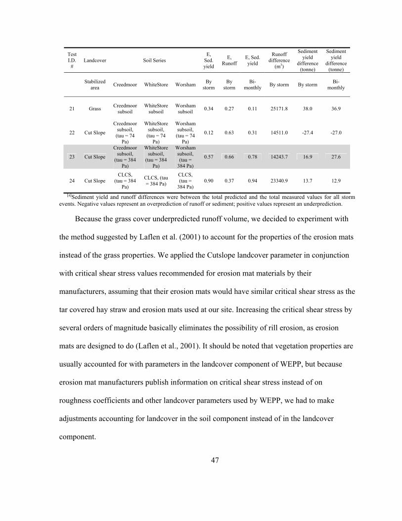
47

Test I.D.

# Landcover Soil Series

E, Sed. yield

E, Runoff

E, Sed. yield

Runoff difference

(m3)

Sediment yield

difference (tonne)

Sediment yield

difference (tonne)

Stabilized area Creedmoor WhiteStore Worsham By

storm By

storm Bi-

monthly By storm By storm Bi-monthly

21 Grass Creedmoor subsoil

WhiteStore subsoil

Worsham subsoil 0.34 0.27 0.11 25171.8 38.0 36.9

22 Cut Slope

Creedmoor subsoil,

(tau = 74 Pa)

WhiteStore subsoil,

(tau = 74 Pa)

Worsham subsoil,

(tau = 74 Pa)

0.12 0.63 0.31 14511.0 -27.4 -27.0

23 Cut Slope

Creedmoor subsoil,

(tau = 384 Pa)

WhiteStore subsoil,

(tau = 384 Pa)

Worsham subsoil, (tau =

384 Pa)

0.57 0.66 0.78 14243.7 16.9 27.6

24 Cut Slope CLCS,

(tau = 384 Pa)

CLCS, (tau = 384 Pa)

CLCS, (tau =

384 Pa) 0.90 0.37 0.94 23340.9 13.7 12.9

[a]Sediment yield and runoff differences were between the total predicted and the total measured values for all storm events. Negative values represent an overprediction of runoff or sediment; positive values represent an underprediction.

Because the grass cover underpredicted runoff volume, we decided to experiment with

the method suggested by Laflen et al. (2001) to account for the properties of the erosion mats

instead of the grass properties. We applied the Cutslope landcover parameter in conjunction

with critical shear stress values recommended for erosion mat materials by their

manufacturers, assuming that their erosion mats would have similar critical shear stress as the

tar covered hay straw and erosion mats used at our site. Increasing the critical shear stress by

several orders of magnitude basically eliminates the possibility of rill erosion, as erosion

mats are designed to do (Laflen et al., 2001). It should be noted that vegetation properties are

usually accounted for with parameters in the landcover component of WEPP, but because

erosion mat manufacturers publish information on critical shear stress instead of on

roughness coefficients and other landcover parameters used by WEPP, we had to make

adjustments accounting for landcover in the soil component instead of in the landcover

component.

48

The critical shear stress for the short term blankets S75, Ds75 produced by North

American Green (tau = 74 Pa) was applied to each subsoil soil series in WEPP, and resulted

in satisfactory runoff efficiency (E = 0.66) and adequate sediment yield efficiency (E = 0.31).

Sediment yields for larger runoff events greatly exceeded measured yields (Figure 2-13),

suggesting that a higher critical shear stress is needed to delay soil detachment. Applying the

critical shear stress of MacMat-vegetated erosion mats produced by Maccaferri Bavions, Inc.

to the same soil series improved model efficiency for sediment yield to exceed our efficiency

target (E = 0.57), most likely because the higher tau value (384 Pa) delayed the release of

sediment to something similar to what was occurring on the site (Figure 2-14).

49

Figure 2-13. Observed and WEPP predicted sediment yield for Carpenter watershed for the post-construction

phase, applying the short term blankets S75, Ds75 critical shear stress value (tau = 74 Pa) .

50

Figure 2-14. Observed and WEPP predicted runoff (a) and sediment yield (b) for Carpenter watershed for the

post-construction phase, applying the MacMat-vegetated erosion blanket critical shear stress value (tau = 384 Pa) .

51

It was noted that bi-monthly and by storm efficiencies were within the same efficiency

class (poor, adequate, or satifactory) for all 4 model simulations with stabilized conditions

(Table 2-6), which was in contrast to simulations with construction site conditions (Table 2-

5). It is not clear why there was a contrast between stabilized and construction conditions.

Watershed delineation by GeoWEPP did not match the watershed boundary from field

observations, with the unexpected removal of a square-shaped piece of land in the lower right

corner of the watershed (Figure 2-15), causing a decrease in size and an alteration of actual

shape of the watershed. The watershed boundaries after clearing and grading were difficult to

delineate because of the installation of storm drains, more shallow and complex changes in

topography, and an increase in impermeable surfaces. GeoWEPP predicted an even

distribution of soil loss between 4 and 12 tonnes ha-1 over most of the watershed, with the

exception of erosion exceeding 16 tonnes ha-1 in and above the channel (Figure 2-15). It was

observed at the site that a gully was forming in the lower half of the channel. Also, because

we did not include the impermeable surfaces of the roads, driveways, and rooftops in the GIS

landcover map, it would be more likely that there would be localized areas of low and

moderate erosion throughout the development.

52

Figure 2-15. GeoWEPP generated annual soil loss map for Carpenter watershed, applying optimal parameters

for the post construction phase. (DEM elevations exaggerated 5X to clearly illustrate topographical characteristics).

PARAMETER RECOMMENDATIONS

A summary of the recommended WEPP parameters based on our findings for the three

construction phases are listed in Table 2-7. For soil series not installed in WEPP, we would

recommend using soil series data from USDA-NRCS, 2002. In addition, Kef, Ki, Kr, and tau

values should be calculated and/or estimated using the WEPP user manual (Alberts et al.,

1995), as it was our experience that WEPP assumes these values to be zero if the "have

model calculate" option in the soil input parameter is selected.

53

Table 2-7. Recommended WEPP soil and landcover parameters for pre-, during, and post-construction phases.

Construction phase Suggested WEPP Soil Inputs Suggested WEPP Landcover inputs

Pre construction (forested and developed arees)

1. WEPP Individual Soil Series 2. Create pavement parameter for impermeable surfaces, applying parameters suggested by Laflen et al. (2001) in Table 2-2

1. WEPP 2yr and 20yr forests for young and mature forests, respectively 2. WEPP Continuous grass for lawn grass 3. WEPP Tall grass for meadows 4. WEPP Cutslope for impermeable surfaces

During construction (graded areas)

1. WEPP Individual Soil Series, A horizon removed and parameters adjusted using WEPP user manual

1. “Baresoil” for all graded areas

Post construction (recently stabilized areas)

1. Same as during construction phase, except tau = 384 for each soil series.

1. WEPP Cutslope for all recently stabilized areas

CONCLUSION

The maximum model efficiency achieved by calibrating GeoWEPP for sediment yield

and runoff volume varied among the three phases of construction. For the pre-construction

phase, the WEPP model adequately predicted runoff volume (E = 0.21) but not sediment

yield (E = -1033.3). Model efficiency for predicting sediment yield improved to -11.16 when

the largest storm event was removed. During construction, we found that the removal of the

A horizon in the soil series soil input parameter and altering specific land cover parameters

resulted in satisfactory runoff (E = 0.78) and sediment yield (E = 0.66). GeoWEPP efficiently

predicted runoff volume (E = 0.66) and sediment yield (E = 0.57) from a residential

development site during post-construction with the application of an erosion blanket critical

shear stress (tau = 384 Pa) in the soil component. Applying the Cutslope landcover with high

critical stress values and the soil series minus A horizon soil parameter, was an effective

method for predicting runoff volume and sediment yield for construction sites in the

stabilization phase.

54

For future work, we would recommend improving WEPP forest parameters to prevent

the underprediction of runoff volume, monitoring sediment yield and runoff volume from

other construction sites to validate our findings, and verifying our post-construction results

with known critical shear stress values of a variety of soils and erosion control products.

REFERENCES

Alberts, E. E., M. A. Nearing, M. A. Weltz, L. M. Risse, F. B. Pierson, X. C. Zhang, J. M.

Laflen, and J. R. Simanton. 1995. Chapter 7. Soil component. In: D. C. Flanagan and

M. A. Nearing (eds.) 1995. USDA-Water Erosion Prediction project: Hillslope profile

and watershed model documentation. NSERL Report No. 10. USDA-ARS National

Soil Erosion Research Laboratory, West Lafayette, IN 47097-1196.

Barton, B. A. 1977. Short-term effects of highway construction on the limnology of a small

stream southern Ontairo. Freshwater Biol. 7: 99-108.

Clesceri, L. S., A. E. Greenberg, and A. D. Eaton (eds.). 1998. Standard methods for the

Examination of Water and Wastewater, 20th ed. American Public Health Association,

American Water Works Association, and Water Environment Federation, pp. 2-57, 2-

58.

Elliot, W. J., and D. E. Hall. 1997. Water Erosion Prediction Project (WEPP) forest

applications. Gen. Tech. Report. INT-GTR-365. Ogden, UT: U.S. Department of

Agriculture, Forest Service, Intermountain Research Station. 11 p.

55

Flanagan, D. C., and M. A. Nearing (eds.). 1995. USDA-Water Erosion Prediction project:

Hillslope profile and watershed model documentation. NSERL Report No. 10. West

Lafayette, IN: USDA-ARS NSERL.

Gilley, J. E., and M. A. Weltz. 1995. Hydraulics of overland flow. In: D. C. Flanagan and M.

A. Nearing (eds.) 1995. USDA-Water Erosion Prediction project: Hillslope profile

and watershed model documentation. NSERL Report No. 10. USDA-ARS National

Soil Erosion Research Laboratory, West Lafayette, IN 47097-1196.

Hogg, I.D., and R.H. Norris. 1991. Effects of runoff from land clearing and urban

development on the distribution and abundance of macroinvertebrates in pool areas of

a river. Aust. J. Mar. Freshwater Res. 42:507-518.

Laflen, J.M., D.C. Flanagan and B.A. Engel. 2001. Application of WEPP to construction

sites. In: (J.C. Ascough and D.C. Flanagan, eds.) Symp. Proc. Soil Erosion Research

for the 21st Century, 3-5 Jan. 2001, Honolulu, HI. Am. Soc. Agric. Eng., St. Joseph,

MI. 135-138.

Lienbow, A. M., W. J. Elliot, J. M. Laflen, and K. D. Kohl. 1990. Interrill erodibility:

Collection and analysis of data from cropland soils. Trans. ASAE. 33(6):1882-1888.

Lindley, M. R., B. J. Barfield, J. C. Ascough II, B. N. Wilson, E. W. Stevens. 1998. The

surface impoundment element for WEPP. Trans. ASAE. 41(3):555-564.

Line, D. E., and N. M. White. 2001. Efficiencies of temporary sediment traps on two North

Carolina construction sites. Trans. ASAE. 44(5):1207-1215.

56

McIsaac, G. F., J. K. Mitchell, J. W. Hummel, and W. J. Elliot. 1992. An evaluation of unit

stream power theory for estimating soil detachment and sediment discharge from

tilled soils. Trans. ASAE. 35(2):535-544.

Nash, J. E., and J. V. Sutcliffe. 1970. River flow forecasting through conceptual models. Part

I - A discussion of principles. J. Hydrology. 10:282-290.

Nearing, M. A., L. Deer-Ascough, and J. M. Laflen. 1990. Sensitivity analysis of the WEPP

hillslope profile erosion model. Trans. ASAE. 33(3):839-849.

Nearing, M. A., D. I. Page, J. R. Simanton, and L. J. Lane. 1989. Determining erodibility

parameters from rangeland field data for a process-based erosion model. Trans.

ASAE. 32(3):919-924.

Neteler, M. and H. Mitasova. 2002. Open Source GIS: A GRASS GIS Approach. Kluwer

Academic Press: Boston, Massachusetts.

Quinton, J. N. 1997. Reducing predictive uncertainty in model simulations: a comparison of

two methods using the European Soil Erosion Model (EUROSEM). Catena.30:101-

117.

Renschler, C. S. 2003. Designing geo-spatial interfaces to scale process models: the

GeoWEPP approach. Hydrol. Process. 17:1005-1017.

Romkens, M. J. M., D. W. Nelson, and C. B. Roth. 1975. Soil erosion on selected high clay

subsoils. J. Soil and Water Conserv. 30(4):173-176.

SAS. 1999. SAS User's Guide: Statistics. Ver. 8.01. Cary, N.C.: SAS Institute, Inc.

57

Savabi, M. R., W. J. Rawls, and R. W. Knight. 1995a. Water erosion prediction project

(WEPP) rangeland hydrology component evaluation on a Texas range site. J. Range

Mgmt. 48:535-541.

Simanton, J. R., M. A. Weltz, and H. D. Larsen. 1991. Rangeland experiments to paramterize

the water erosion prediction project model: vegetation canopy cover effects. J. Range

Mgmt. 44(3):276-282.

S.C.O.N.C. 2004. State Climate Office of North Carolina. Available at http://www.nc-

climate.ncsu.edu/.

Taylor, B. C., and J. C. Roff. 1986. Long-term effects of highway construction on the

ecology of a southern Ontario stream. Environ. Pollution Ser. A. 40:317-344.

Toy, T.J, and R.F. Hadley. 1987. Geomorphology and reclamation of disturbed lands. San

Diego, California: Academic Press.

U. S. Environmental Protection Agency. 1976. Loading functions for assessments of water

pollution from non-point sources. EPA-600/2-76-151. Washington D.C.: US. E.P.A.

USDA - NRCS. 1997. A geography of hope. U.S. Government Printing Office. Washington,

D.C.

USDA - NRCS. 2000. Soil Survey Geographic (SSURGO) Data. Available at:

http://www.ncgc.nrcs.usda.gov/branch/ssb/products/ssurgo/.

USDA - NRCS. 2002. Official Soil Series Descriptions: Soil Survey Division, Natural

Resources Conservation Service, United States Department of Agriculture. Available

at: http://soils.usda.gov/technical/classification/osd/index.html.

58

Wilcox, B. P., M. Sbaa, W. H. Blackburn, and J. H. Milligan. 1992. Runoff prediction from

sagebrush rangelands using water erosion prediction project (WEPP) technology. J.

Range Mgmt. 45(5):470-474.

Wolman, M.G., and A.P. Schick. 1967. Effects of construction on fluvial sediment, urban

and suburban areas of Maryland. Water Resources Res. 3(2):451-464.

Zhang, X. C., M. A. Nearing, and L. M. Risse. Estimation of Green-Ampt conductivity

parameters: Part I. Row crops. Trans. ASAE. 38(4):1069-1077.

Zhang, X. C., M. A. Nearing, and L. M. Risse. Estimation of Green-Ampt conductivity

parameters: Part II. Perennial crops. Trans. ASAE. 38(4):1079-1087.

59

APPENDIX

Figure A2-1. Soil grid map at 7 m resolution for watersheds Centennial A (above) and Centennial C (below).

Watersheds are divided into three hillslopes by GeoWEPP.

60

Figure A2-2. Digital elevation model at 7 m resolution for watersheds Centennial A (above) and Centennial C

(below). Watersheds are divided into three hillslopes by GeoWEPP.

61

Figure A2-3. Soil grid map at 5 m resolution for the Carpenter watershed during construction. The watershed

is divided into three hillslopes by GeoWEPP.

62

Figure A2-4. Soil grid map at 5 m resolution for the Carpenter watershed during construction. The watershed

is divided into three hillslopes by GeoWEPP.

63

Table A2-1. Rainfall, runoff, and sediment measurements from selected storm events at Centennial watersheds A &

C.

Date Watershed Rainfall amount (mm)

Peak rainfall intensity (mm/hr)

Runoff (m^3) TSS (kg)

1/23/02 A 32.8 13.2 17.3 140

3/21/02 A 10.7 4.1 3.4 10

3/26/02 A 18.3 57.9 21.9 99

8/30/02 A 27.9 21.3 397.2 47

10/11/02 A 109.7 57.1 2536.8 318

10/29/02 A 4.3 7.1 164.7 40

11/6/02 A 23.9 35.6 6.1 33

11/17/02 A 24.1 5.1 307.0 34

1/23/02 C 32.8 2.5 547.0 224

3/31/02 C 47.5 61.9 1097.4 119

10/30/02 C 10.4 7.62 285.0 26

11/6/02 C 23.9 8.9 390.0 128

11/12/02 C 21.1 28.4 535.0 220

64

Table A2-2. Rainfall, runoff, and sediment measurements from selected storm events at Carpenter watershed.

Date Construction phase Rain (mm) Runoff (m^3) TSS (kg) Estimated sediment trap efficiency (%)

TSS + trap sediment (kg)

12/10/97 During 13.2 60.6 8.4 59[a] 20.4 12/22/97 During 20.6 535.6 1385.1 59[a] 3353.8 12/24/97 During 13.0 277.5 717.6 59[a] 1737.6 12/27/97 During 22.6 604.4 1563.1 59[a] 3784.9 1/8/98 During 18.8 789.6 4089.9 59[a] 9902.8 1/15/98 During 53.6 1546.4 8710.3 59[a] 21090.3 1/18/98 During 24.9 745.9 2968.4 59[a] 7187.5 1/22/98 During 29.7 1097.3 2114.0 59[a] 5118.7 1/27/98 During 47.2 1439.1 4834.7 59[a] 11706.3 2/3/98 During 23.4 630.3 1462.1 59[a] 3540.1 2/16/98 During 58.7 2234.3 4390.0 59[a] 10629.4 2/22/98 During 11.7 286.7 461.5 59[a] 1117.5 3/8/98 During 60.5 1886.5 2739.8 59[a] 6633.9 3/17/98 During 26.9 1022.6 1485.2 59[a] 3596.2 3/18/98 During 98.8 3185.7 4626.7 59[a] 11202.7 4/4/98 During 11.1 225.9 328.0 59[a] 794.3 4/9/98 During 22.4 595.8 771.5 59[a] 1868.1 5/7/98 During 21.6 374.2 484.6 59[a] 1173.4 5/11/98 During 29.0 417.5 540.6 59[a] 1309.1 5/23/98 During 17.0 415.2 1755.9 59[a] 4251.7 6/3/98 During 20.1 567.8 570.6 59[a] 1381.6 6/15/98 During 26.7 870.6 5205.9 59[a] 12605.1 7/4/98 During 38.9 1155.1 6108.8 77 26559.8 7/27/98 During 20.3 385.3 3632.8 49 7123.2 7/30/98 During 15.7 236.1 1119.2 49 2194.5 8/9/98 During 39.9 809.3 7647.6 49 14995.2 8/10/98 During 11.2 157.1 1485.0 49 2911.8 8/16/98 During 41.2 927.0 13124.6 49 25734.5 9/3/98 During 61.7 682.2 2455.7 71 8467.9 9/8/98 During 12.2 65.1 234.4 71 808.2 10/4/98 During 15.2 124.6 617.8 71 2130.5 10/8/98 During 40.9 977.7 8564.1 71 29531.4 11/3/98 During 24.4 485.7 862.0 23 1119.4 11/4/98 During 10.9 367.6 453.9 23 589.5 11/14/98 During 9.4 198.1 268.4 23 348.6 11/16/98 During 12.9 229.2 310.5 23 403.2 11/26/98 During 5.6 36.0 37.9 23 49.3 12/13/98 Stabilization 21.6 765.5 235.2 23 305.4 12/16/98 Stabilization 17.3 423.8 226.1 23 293.7 12/24/98 Stabilization 33.0 957.2 510.8 23 663.4 1/2/99 Stabilization 45.0 1358.5 1281.0 23 1663.6 1/15/99 Stabilization 10.7 189.2 127.5 69 411.3 1/18/99 Stabilization 16.0 391.5 882.7 69 2847.4 1/23/99 Stabilization 52.3 1650.0 1240.7 69 4002.2 2/1/99 Stabilization 14.2 191.9 63.7 69 205.5 2/17/99 Stabilization 14.2 135.3 83.9 18 102.3 2/19/99 Stabilization 10.9 282.1 213.0 18 259.7 3/14/99 Stabilization 40.9 910.0 1022.7 18 1247.2 3/21/99 Stabilization 27.9 545.5 523.6 18 638.6 4/1/99 Stabilization 21.6 410.4 473.1 18 577.0 4/30/99 Stabilization 42.2 876.3 455.6 18 555.7 7/13/99 Stabilization 36.1 483.2 306.6 47 578.5 8/14/99 Stabilization 34.8 423.2 1498.1 47 2826.7 8/26/99 Stabilization 21.6 369.2 609.0 47 1149.1 9/4/99 Stabilization 168.2 5534.6 9237.0 18 11264.6 9/15/99 Stabilization 123.4 4020.3 4694.2 18 5724.6 9/22/99 Stabilization 15.7 372.1 213.6 18 260.5 9/27/99 Stabilization 43.7 1318.6 819.1 18 998.9

65

Date Construction phase Rain (mm) Runoff (m^3) TSS (kg) Estimated sediment trap efficiency (%)

TSS + trap sediment (kg)

9/28/99 Stabilization 33.0 957.2 315.8 18 385.2 9/30/99 Stabilization 19.6 501.2 299.4 18 365.2 10/17/99 Stabilization 34.8 1017.4 122.1 18 148.9 10/20/99 Stabilization 12.7 252.5 52.0 18 63.4 11/2/99 Stabilization 8.1 122.0 39.8 18 48.5 11/26/99 Stabilization 18.3 404.1 357.7 18 436.3 12/13/99 Stabilization 29.7 917.6 1021.5 18 1245.7 1/9/00 Stabilization 38.3 1246.9 1832.8 18 2235.1 1/20/00 Stabilization 15.2 439.1 65.4 18 79.8 1/24/00 Stabilization 54.1 1121.5 167.1 18 203.8 1/30/00 Stabilization 27.7 776.5 71.4 18 87.1 2/12/00 Stabilization 19.0 484.0 55.8 18 68.0 2/27/00 Stabilization 15.7 359.1 53.5 18 65.2 3/27/00 Stabilization 12.4 416.4 149.7 59[a] 362.4 4/8/00 Stabilization 15.7 394.1 224.6 59[a] 543.9 4/15/00 Stabilization 14.5 292.5 134.5 59[a] 325.8 4/18/00 Stabilization 15.2 378.5 401.2 59[a] 971.5 4/25/00 Stabilization 13.7 228.4 226.1 59[a] 547.5

[a] Sediment trap efficiency based on overall efficiency average.

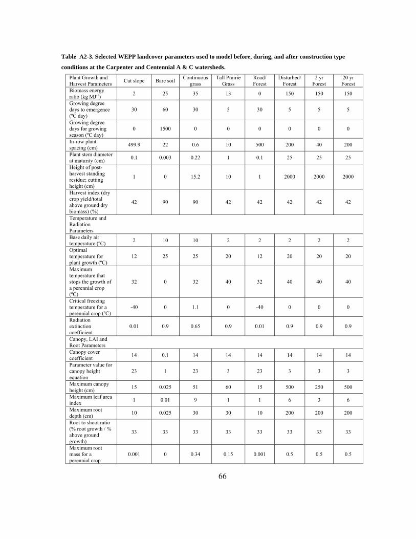
66

Table A2-3. Selected WEPP landcover parameters used to model before, during, and after construction type

conditions at the Carpenter and Centennial A & C watersheds.

Plant Growth and Harvest Parameters Cut slope Bare soil Continuous

grass Tall Prairie

Grass Road/ Forest

Disturbed/ Forest

2 yr Forest

20 yr Forest

Biomass energy ratio (kg MJ-1) 2 25 35 13 0 150 150 150

Growing degree days to emergence (ºC day)

30 60 30 5 30 5 5 5

Growing degree days for growing season (ºC day)

0 1500 0 0 0 0 0 0

In-row plant spacing (cm) 499.9 22 0.6 10 500 200 40 200

Plant stem diameter at maturity (cm) 0.1 0.003 0.22 1 0.1 25 25 25

Height of post-harvest standing residue; cutting height (cm)

1 0 15.2 10 1 2000 2000 2000

Harvest index (dry crop yield/total above ground dry biomass) (%)

42 90 90 42 42 42 42 42

Temperature and Radiation Parameters

Base daily air temperature (ºC) 2 10 10 2 2 2 2 2

Optimal temperature for plant growth (ºC)

12 25 25 20 12 20 20 20

Maximum temperature that stops the growth of a perennial crop (ºC)

32 0 32 40 32 40 40 40

Critical freezing temperature for a perennial crop (ºC)

-40 0 1.1 0 -40 0 0 0

Radiation extinction coefficient

0.01 0.9 0.65 0.9 0.01 0.9 0.9 0.9

Canopy, LAI and Root Parameters

Canopy cover coefficient 14 0.1 14 14 14 14 14 14

Parameter value for canopy height equation

23 1 23 3 23 3 3 3

Maximum canopy height (cm) 15 0.025 51 60 15 500 250 500

Maximum leaf area index 1 0.01 9 1 1 6 3 6

Maximum root depth (cm) 10 0.025 30 30 10 200 200 200

Root to shoot ratio (% root growth / % above ground growth)

33 33 33 33 33 33 33 33

Maximum root mass for a perennial crop

0.001 0 0.34 0.15 0.001 0.5 0.5 0.5

67

Plant Growth and Harvest Parameters Cut slope Bare soil Continuous

grass Tall Prairie

Grass Road/ Forest

Disturbed/ Forest

2 yr Forest

20 yr Forest

(kg/m^2)

Senescence Parameters

Percent of growing season when leaf area index starts to decline

85 70 85 25 85 25 25 25

Period over which senescence occurs (days)

14 14 14 40 14 300 200 300

Percent canopy remaining after senescence

0.1 75 70 30 0.1 50 50 50

Percent of biomass remaining after senescence

1 70 90 25 1 70 70 70

Residue parameters Parameter for flat residue cover equation (m2 kg-1)

5 5 5 5 5 5 5 5

Standing to flat residue adjustment factor (wind, snow, etc.) (%)

99 99 99 99 99 99 99 99

Decomposition constant to calculate mass change of above-ground biomass

0.0074 0.0065 0.009 0.0068 0.0074 0.006 0.006 0.006

Decomposition constant to calculate mass change of root biomass

0.0074 0.0074 0.009 0.0068 0.0074 0.006 0.006 0.006

Use fragile or non-fragile mfo values Non-fragile Non-

fragile Non-

fragile Non-fragile Non-fragile

Non-fragile

Non-fragile

Non-fragile

Other Parameters

Plant specific drought tolerance (% of soil porosity)

10 0 0 10 10 10 10 10

Critical live biomass value below which grazing is not allowed (kg m-2)

0 0 0.1 0 0 0 0 0

Maximum Darcy Weisbach friction factor for living plant

1 0 12 11 1 17 15 17

Harvest Units Wepp WillSet

Wepp WillSet

Wepp WillSet

Wepp WillSet

Wepp WillSet

Wepp WillSet

Wepp WillSet

Wepp WillSet

Optimal yield under no stress conditions (kg m-2)

0 0 0 0 0 0 0

68

Plant Growth and Harvest Parameters Cut slope Bare soil Continuous

grass Tall Prairie

Grass Road/ Forest

Disturbed/ Forest

2 yr Forest

20 yr Forest

Bulk density after tillage (g cm-3) 1.0 1.6 1.1 1.1 1.0 1.1 1.1 1.1

Initial canopy cover (%) 0 0 50 30 0 90 50 90

Days since last tillage 0 200 200 1000 0 1000 1000 1000

Days since last harvest 0 2000 92 900 0 100 100 100

Initial frost depth (cm) 0 0 0 0 0 0 0 0

Initial interrill cover (%) 0 0 50 80 0 100 20 100

Initial residue cropping system Fallow Fallow Perennial Perennial Fallow Perennial Perennial Perennial

Cumulative rainfall since last tillage (mm)

420.1 19.69 500 1000 420.1 1000 1000 1000

Initial ridge height after last tillage (cm)

0.6 0 2 10 0.6 10 10 10

Initial rill cover (%) 0 0 50 80 0 100 20 100

Initial roughness after last tillage (cm)

0.6 0.1 2 10 0.6 10 10 10

Rill spacing (cm) 400.1 0 0 0 400.1 0 0 0

Rill width type Temporary Temp Temp Temp Temp Temp Temp Temp Initial snow depth (cm) 0 0 0 0 0 0 0 0

Initial depth of thaw (cm) 0 0 0 0 0 0 0 0

Depth of secondary tillage layer (cm) 2.54 3.937 10 10 2.54 10 10 10

Depth of primary tillage layer (cm) 2.54 7.874 20 20 2.54 20 20 20

Initial rill width (cm) 0 0 0 0 0 0 0 0

Initial total dead root mass (kg m-2) 0 0 0.2 0.1 0 0.5 0.5 0.5

Initial total submerged residue mass (kg m-2)

0 0 0 0.1 0 0.5 0.5 0.5

69

Chapter 3: Applying Process-Based Models for Erosion

and Sediment Control Design

ABSTRACT. Sediment and erosion controls have been required on construction sites for many years,

but are often not very effective in reducing sediment movement to streams. One approach to investigating the

effectiveness of erosion and sediment controls is to use computer models to evaluate the individual and

combined effect of sediment control measures. WEPP and GeoWEPP models were applied to determine the

efficiency of planned controls on construction sites, and to create Best Management Practices (BMP) scenarios

to meet North Carolina water quality standards. Two small watersheds (A & C) with plans for construction in

Raleigh, NC were selected for modeling. Two sediment traps on watershed A were modeled as impoundments in

WEPP, and a 15.2 m wide forested riparian buffer on watershed C was modeled with GeoWEPP. WEPP

estimated trapping efficiencies within NC standards of 70 % trapping efficiency for particle sizes greater than

0.04 mm. WEPP predicted that the turbidity of runoff from the second sediment trap at the site outlet would be

equal to or less than NC turbidity requirements of 50 Nephlometric Turbidity Units for 11 % of storm events.

Turbidity standards were met on watershed A essentially by capturing the storm runoff, which was done by

removing the outlet from sediment trap B and increasing the trap area 6-fold from 1 % to 8 % of the drainage

area. Replacing rock check dams with culverts greatly reduced TSS concentrations, although the average

turbidity level of 50 NTUs still exceeded standards. The GeoWEPP model predicted that planned riparian

buffer would not meet the turbidity standard for any of the modeled storm event unless combined with other

BMPs. Extending the design buffer in Watershed C decreased TSS concentration predicted with the design

buffer by 57 %, while only increasing vegetation space on the construction site from 13 % to 22 %. Maintaining

forested areas on highly erosive areas surprisingly had little impact on runoff volume or sediment yield, which

may suggest a potential flaw within the GeoWEPP model.

Keywords. Erosion, Construction, Watershed, BMP, sediment, riparian buffer, WEPP model, GeoWEPP,

GIS, Sediment, Runoff.

70

Introduction

Because land-developing activities require vegetation removal and landscape reshaping,

the soil surface is exposed to the elements and subjected to erosion. By 1980, construction

activities had disturbed an estimated 1.7% of U.S. land (Toy and Hadley, 1987). Toy and

Hadley (1987) also noted that land disturbance from mining, residential, commercial and

highway construction can accelerate erosion by two or more orders of magnitude. In 1973,

the Clean Water Act placed the responsibility of maintaining water quality from construction

sites on state governments (Title II, section 208). In response, the state of North Carolina

passed the Sedimentation Pollution Control Act of 1973, which required the approval of

erosion control plans by the Sediment Control Commission of NC (NC General Statutes,

1973), with the distinction that discharge from the site would not exceed a turbidity of 50

Nephlometer Turbidity Units (NTUs). It was also stated that sediment traps are required to

have 70 % settling efficiency for particles greater than or equal to 0.04 mm in diameter for a

2-year storm, which is 88.9 mm in Raleigh, NC.

To meet these standards, land developers and contractors must install sediment and

erosion controls on their sites. Optimal placement of controls is dependent on topography,

soil, and landcover. The traditional method for designing erosion and sediment control plans

has been based on visual interpretations of contour maps, soil survey maps, and field surveys

(Goldman et al., 1986). This method is labor and time intensive, and heavily dependent on

the competency of the designer. Also, it can be difficult to account for interactions between

elevation, soil, and landcover. Another method is computer erosion prediction modeling,

which allows the user to identify erosive areas and to compare the effectiveness of different

71

control measures (Goldman et al., 1986). Process-based erosion prediction models attempt to

simulate significant processes going on in the environment by applying laws and theories of

physical movement, and can be easily applied to a large variety of landscapes and situations

(Doe and Harmon, 2001).

The Water Erosion Prediction Project, or WEPP, is a lumped-parameter process-

based model designed to simulate erosion and deposition on agricultural areas, and is one of

the most widely studied process-based erosion prediction models in current use (Flanagan

and Nearing, 1995). The watershed version of WEPP can be used to simulate sediment

controls such as sediment traps, rock check dams, and emergency spillways (Lindley et al.,

1998). GeoWEPP, which provides a geographical information system GIS interface for

WEPP, can be used to account for spatially variable erosion controls such as vegetative

buffers, erosion mats on steeper slopes, and staged construction (Renschler, 2003).

GIS can also be used for designating optimal placement of BMPs (Best Management

Practices) on watersheds. Tomer et al. (2003) applied GIS to determine optimal buffer width

and placement for reducing nutrients in streams by designating riparian grid cells with large

upslopes and low slopes as optimal sites for buffer placement.

There are several examples of computer models applied by researchers to test the effect

of BMPs on controlling pollutants. Yuan et al. (2001) applied Ann AGNPs Annualized

Agricultural Non-Point Source to test impoundments and winter cover crops as BMPs for

reducing sediment loads on a large watershed. Wright et al., 1992, used CREAMS-

DRAINMOD (Chemicals, Runoff, and Erosion from Agricultural Management Systems -

Drainage Simulation Model) to evaluate the effects of different types of water table

72

management runoff, erosion, and nitrogen losses. Gerwig et al., 2001 examined the effect of

riparian buffers using GLEAMS (Groundwater Loading Effects of Agricultural Management

Systems) and REMM (Riparian Ecosystem Management Model) on phosphorous and

nitrogen transport from agricultural fields receiving swine effluent.

The objective of this research is to experiment with WEPP and GeoWEPP as land

planning tools by determining the efficiency of planned erosion and sediment controls on

sample construction sites, applying erosion controls to erosive areas designated by

GeoWEPP, and creating BMP scenarios on sample construction sites to meet North Carolina

water quality standards.

METHODS AND MATERIALS

SITE DESCRIPTION

Two watersheds in Wake County, NC, were selected for modeling purposes. Detailed

site descriptions are listed in Table 3-1. Both watersheds (referred to as watersheds A & C)

are located on North Carolina State University's Centennial Campus in Raleigh, NC.

Watershed A was modeled using erosion and sediment control plans that were applied during

the development of the Centennial Campus Middle School. The N.C. Sediment Control

Commission (1988) state that sediment storage volume must be at least 126 m3 ha-1 of the

total disturbed area draining into the sediment trap. Thus, sediment trap A had storage

volume of 165 m3 for a drainage area of 1.31 ha and sediment trap B had storage volume of

281.4 m3 for a drainage area of 2.23 ha (Figure 3-1). Both sediment traps contain rock check

dam outlets. Watershed C was modeled using projected erosion control plans for the

73

development of the Centennial Campus Golf Course. Because of the presence of streams,

these plans included a 15.2 m width of undisturbed forested buffer from the perennial portion

of the stream to remain during and after construction in order to comply with Neuse Buffer

Rules (Figure 3-1).

Table 3-1. General site description of watersheds A & C on North Carolina State University's Centennial Campus in

Raleigh, North Carolina.

Watershed A Watershed C Elevation

above mean sea level (m)

98 - 115 97 - 128

Area (ha) 9.3 11.8

Soil 13 % Pavement 29 % Appling

58 % Cecil

1 % Pavement 90 % Cecil 9 % Colfax

Construction period 1998 - 1999 Pending

74

Figure 3-1. Landcover during construction on watersheds A (upper) and C (lower) watersheds A & C on North

Carolina State University's Centennial Campus in Raleigh, North Carolina.

75

MODEL DESCRIPTIONS

WEPP

Water Erosion Prediction Project (WEPP) is a lumped parameter, one-dimensional,

process-based erosion model that simulates the detachment, transport, and deposition of

sediment on rectangular hillslopes during runoff events, predicting sediment yield and runoff

volume during storm events (Flanagan and Nearing, 1995). Figure 3-2 illustrates how

landcover in Watershed A is simplified into one lumped parameter for each hillslope in

WEPP. General soil, landcover, and slope information for each hillslope is listed in Table

A3-1.

Figure 3-2. WEPP Watershed view of the three hillslopes (H1, H2, and H3), two channels (C1 and C2), and two

impoundments (I1 and I2) modeled in watershed A. Hillslopes H1 and H2 are orange to represent exposed soil;

hillslope H3 is green to represent forest.

76

WEPP has been validated for agricultural fields, (Zhang et al., 1995a; Zhang et al.,

1995b; McIsaac et al., 1992; Lienbow et al., 1990), rangelands (Savabi et al., 1995; Simanton

et al., 1991; Wilcox et al., 1990; Nearing et al., 1989), impoundments (Lindley et al., 1998),

and calibrated for forested areas (Elliot and Hall, 1997). Watershed A was modeled using

WEPP Watershed Version 2002.70, which provides input parameters for impoundments with

outlet structures such as culverts, rock check dams, and straw bales. Sedimentation

algorithms for WEPP impoundments were developed by Lindley et al. (1998) and are based

upon principle of conservation of mass for as follows:

dtdDepCQCQ

dtdM

OOii −−= (1)

where

M = Mass in the impoundment (kg)

Ci = Incoming sediment concentration (kg m-3)

Co = Outgoing sediment concentration (kg m-3)

Dep = Deposition (kg)

Qi = Inflow rate (m3 sec-1)

Qo = Outflow rate (m3 sec-1)

While sediment algorithms apply to all impoundments, flow rate equations in WEPP are

specific to impoundment outlets. Figure 3-3 illustrates the equation used to predict flow rates

for the rock check dam outlets in sediment traps A & B.

77

b

RFRFRF aL

HWQ/1

⎥⎦

⎤⎢⎣

⎡=

QRF - Flow rate through check dam (m3 s-1) WRF - Cross-sectional width of check dam (m) H - Head loss through check dam (HOTRF - HRF) (m) LRF - Average flow length of rock check dam (m) a and b- Coefficients, function of rock diameter (DRF) and flow length (LRF)

Figure 3-3. Schematic of the rock check dam impoundment as modeled by WEPP (from Lindley et al., 1998).

GeoWEPP

GeoWEPP ArcX 2004.3 is an ESRI-ArcView extension that directly links GIS to WEPP

(Renschler, 2003). GeoWEPP allows the user to model raster cells as individual hillslopes,

thus accounting for spatial variability among slope, soils, and landcover. Although currently

GeoWEPP is not designed to simulate impoundment hydrology, it is an effective tool for

detecting specific erosive and depositional areas around vegetative BMPs such as riparian

buffers. It should also be noted that GeoWEPP is not a validated model, and therefore must

be validated by the individual user. As the primary BMP for Watershed C was a forested

78

buffer, erosion processes were simulated using GeoWEPP. Figure 3-4 illustrates how

landcover in Watershed C is distributed into one parameter for each raster cell in GeoWEPP.

Figure 3-4. Landcover input map for GeoWEPP simulating a forested buffer designed to meet Neuse River

Basin Rules, on Watershed C during construction.

MODEL INPUTS

WEPP

Climate, soil, landcover, and slope input are required by WEPP for modeling. Input

parameters for both WEPP and GeoWEPP simulations were created in WEPP. All climate

information was retrieved from the RDU airport weather station for the years of 1998 and

1999 for both watersheds and submitted into WEPP CLIGEN format (Table A3-2) (SCONC,

2004). The climate parameter also includes climate data for 1997, to allow the water balance

79

to equilibrate before modeling the target storm events. Soil parameter information required

by WEPP is listed in Table 3-2. Appling and Cecil soil series were not included in the WEPP

database, therefore soil parameters originating from these series were created using the

NRCS soil series descriptions (USDA - NRCS, 2002) and equations from the WEPP manual

(Alberts et al., 1995).

Table 3-2. WEPP input soil parameters for watersheds A & C on North Carolina State University's Centennial

Campus in Raleigh, North Carolina.

Soil description

Soil Texture[a]

Interrill erodibility

(Ki)

Rill erodibility

(Kr)

Critical shear stress (tau)

Effective Hydraulic

conductivity Kef

Sand Clay CEC Rock

kg sec m-4 sec m-1 Pa mm h-1 % % meq/ 100 g %

Appling SL 4.97 x 106 1.02 x 10-2 2.5 4.4 65 15 3.0 3

Appling subsoil CL 4.31 x 106 4.80 x 10-3 4.7 4.4 45 40 8.0 4

Cecil L 5.43 x 106 8.50 x 10-3 3.3 4.8 50 12 7.3 3

Cecil subsoil L 5.43 x 106 8.50 x 10-3 3.3 4.4 45 25 5.5 4

Colfax L 5.31 x 106 7.00 x 10-3 3.1 7.1 41 19 7.3 3

Colfax subsoil L 5.31 x 106 7.00 x 10-3 3.1 7.1 48 27 5.5 4

Pavement SL 1.00 x 103 1.00 x 10-4 100.0 0.1 10 70 25 90 [a] SL - Sandy loam, L - Loam, CL - Clay loam

Complete WEPP landcover input parameters are listed in Table A3-3. Select WEPP

landcover parameters in Table 3-3 were chosen based on degree of sensitivity, using

parameters as suggested by Nearing et al., 1990. In Chapter 2, we found that the subsoil soil

series input parameters used in combination with the WEPP landcover "Cutslope" parameter

resulted in a satisfactory runoff efficiency (E = 0.78) when compared to measured runoff data

from a construction site near Raleigh, NC. Construction site soil conditions were modeled

using soils on Watersheds A & C altered in this manner. Forest and tall grass landcover

parameters from WEPP were selected based on the highest runoff efficiency achieved (E =

80

0.21) for stable watersheds, as determined in Chapter 2. Slope information was derived

manually from contour maps of the area, assuming a simple uniform slope for each hillslope.

Table 3-3. Selected WEPP landcover input parameters for watersheds A & C on North Carolina State University's

Centennial Campus in Raleigh, North Carolina.

Plant Growth and Harvest Parameters

Cut slope

Tall Prairie Grass Disturbed/Forest

Maximum Darcy Weisbach friction factor

for living plant 1 11 17

Initial canopy cover (%) 0 30 90

Days since last tillage 0 1000 1000

Days since last harvest 0 900 100

Initial interrill cover (%) 0 80 100

Initial residue cropping system Fallow Perennial Perennial

Initial rill cover (%) 0 80 100

Initial roughness after last tillage (cm) 0.6 10 10

Initial total dead root mass (kg m-2) 0 0.1 0.5

Sediment trap information was imported from the sediment trap characteristics in the

erosion and sediment control design for the Centennial Campus Middle School (Table 3-4).

Check dam length and cross-sectional width was based on the minimum requirements in the

NC Sediment and Erosion Control Design Manual. The infiltration rate of the sediment traps

was assumed to be the same as infiltration rates for the Cecil subsoils on this site.

81

Table 3-4. WEPP impoundment inputs for designed sediment traps A & B on North Carolina State University's

Centennial Campus in Raleigh, North Carolina.

WEPP Impoundment inputs Sediment trap A Sediment trap B

LRF (m) 1.52 1.52

HRF (m) 0.0 0.0

WRF (m) 1.52 1.52

DRF (m) 0.23 0.23

HOTRF (m) 0.91 1.52

HFULL (m) 0.46 0.76 Infiltration rate (Qinf) (m day-1) 0.11 0.11

Bottom stage area (m2) 131.5 105.9

Top stage area (m2) 237.5 286.1

Bottom stage length (m) 18.0 17.4

Top stage length (m) 21.6 23.5

GeoWEPP

Data layers for GeoWEPP Arc X 2004.3 were constructed and modified using ArcView

GIS 3.2a and GRASS 5.0. The digital elevation models (DEMs) were created by

implementing a spline algorithm in GRASS (Neteler and Mitasova, 2000) to interpolate 2 ft

(0.6 m) interval contour maps to 7 m resolution grids for both watersheds. Soil maps, scaled

at 1:24,000, were downloaded from the USDA-NRCS Soil Survey Geographic Database

(Figure A3-1) (USDA-NRCS, 2000). The landcover map for watersheds A & C watersheds

was derived from aerial photos of the site. Soil, landcover, and DEMs were exported from

grid format to the ASCII format required by GeoWEPP.

METHODS FOR OPTIMIZING BMPS

New erosion control plans for Watersheds A & C were created with the goal of meeting

NC standards for sediment. Specifically, our goal was to reduce turbidity levels to 50 NTUs

in runoff leaving the site, and to design sediment traps with a minimum of 70 % retention

82

efficiency as mandated by the Sediment Control Act of NC. A second-order polynomial was

developed with the SAS procedure PROC NLIN using TSS and turbidity data retrieved from

1/23/02 to 4/1/02 (Figure 3-5) (SAS, 1999). Following this relationship, TSS concentrations

of 16.6 mg L-1 were assumed to be equivalent to 50 NTUs, with the understanding that their

TSS concentrations range greatly at each turbidity level. In this case TSS concentrations

ranged from 2.0 to 22.7 mg L-1 for turbidity values between 45 and 55 NTUs.

Figure 3-5. Relationship between TSS and turbidity in runoff samples collected from outlets on watersheds A

& C on North Carolina State University's Centennial Campus in Raleigh, North Carolina.

GeoWEPP was applied to create erosion control coverage on the Watershed C

construction site in areas of high soil loss, with the objective of optimizing the efficiency of

vegetative cover by allowing the existing forest to remain standing on the most erosion

sensitive areas on the site. GeoWEPP simulations were used to identify erosive areas,

83

applying a landcover input map representing the construction site without vegetated buffers.

Cells that had an estimated soil loss greater than either 128 or 256 tonnes ha-1 were used to

create forested areas on the landcover input map (Figure 3-6). These soil loss tolerance levels

were selected to simulate what we considered to be the upper and lower limits of maintaining

a reasonable amount of space for construction while significantly reducing erosion losses,

and were labeled as high and low cover, respectively. To save on time and effort, the

newlandcover.aml script was developed to convert highly erosive cells from GeoWEPP

output map to landcover on high erosion areas in the landcover input map, based on a soil

loss tolerance which can be determined by the user (Script A3-1).

84

Figure 3-6. Creating landcover on high erosion areas detected by GeoWEPP.

84

85

RESULTS AND DISCUSSION

EFFICIENCY OF PLANNED BMPS

WEPP Impoundments

Trap efficiency, average TSS, peak outflow, inflow and outflow runoff volumes, and

number of days that traps were overtopped were estimated on a yearly basis using WEPP

(Table 3-5). Yearly output was averaged over 1998 and 1999, because there was little

difference between them. Both sediment traps were predicted to have greater than 70 %

trapping efficiencies for particle sizes larger than 0.05 mm in diameter (Table 3-5),

suggesting that the sediment traps would have been within NC sediment trap efficiency

standards. Sediment trap A had a higher trapping efficiency than trap B, despite the fact that

sediment B was 1.7 times larger in storage volume than sediment trap A. Peak outflow rates

were 8 times greater for trap B than trap A (Table 3-5), as sediment trap B received water

from sediment trap A in addition to water from its own surrounding drainage area (Figure 3-

2), which would reduce sediment settling. It should be noted that Line and White (2001)

measured an average sediment trap efficiency of 59 % from a standard-sized trap on a

construction site in Wake County, N.C., similar to what we predicted for total sediment trap

efficiency in sediment trap B.

86

Table 3-5. WEPP impoundment output averaged over 1998 and 1999 precipitation events on watersheds A & C on

North Carolina State University's Centennial Campus in Raleigh, North Carolina.

Trap

efficiency (%)

Trap efficiency, particles > 0.05

mm

Avg. TSS, outflow

(mg L-1 )

Peak outflow rate (m3 sec-1)

Total inflow volume

(m3)

Total outflow volume

(m3)

# Days overtopped

Sediment trap A 85 92.0 3460 0.114 2790.0 2781.3 2

Sediment trap B 52 74.1 1400 0.908 6329.2 6319.2 3

TSS concentration was predicted on a storm event basis for both sediment traps. WEPP

produces output for watersheds with impoundment outlets on a yearly basis, and on an event-

by-event basis for channel outlets. To produce sediment yield information on a storm event

basis from sediment trap B, a small channel with a length of 1.5 m was attached to the outlet

of sediment trap B in the model. This allowed WEPP to produce sediment yield results for

runoff exiting sediment trap B for individual storms (Figure 3-2).

WEPP predicted that runoff leaving the construction site from sediment trap B would

meet turbidity standard of 50 NTUs for only 11 % of the 53 storm events that occurred from

1998 to 1999 (Figure 3-7). Acceptable turbidity levels were predicted to occur during light

precipitation events (20 mm or less). When the site was modeled without sediment traps,

turbidity levels exceeded 50 NTUs for all storm events. From these results we concluded that

while the sediment traps could potentially reduce sediment yields and would most likely

meet NC trap efficiency standards, they would not be effective for meeting NC turbidity

standards without additional BMPs.

87

Figure 3-7. Predicted TSS in outlet directly below sediment trap B during construction, with and without the

addition of two planned sediment traps.

GeoWEPP Vegetation

The GeoWEPP model predicted that the planned forested riparian buffers were not able

to meet the NC 50 NTU turbidity standard for storm events that occurred during 1998 and

1999, with the lowest turbidity of 715 NTUs (304 mg L-1) occurring during a snow melt

event (Figure 3-8). The addition of the design buffer did reduce TSS concentrations for all

storms by 62 % and sediment yield by 47 % compared to no buffer at all, illustrating that the

forested buffers would significantly reduce sediment loads entering the stream. These

sediment capture rates are similar to those found in sediment traps (Line and White, 2001),

suggesting that maintaining natural vegetation around stream banks on developing sites

would be as effective for reducing sediment yields as installing sediment traps. However,

assuming GeoWEPP estimates are valid, the 15.2 m wide buffer required for this site would

88

most likely need to be used in combination with impoundments such as sediment traps and

check dams to meet the state water quality standard.

Figure 3-8. Predicted TSS in Watershed outlet C during construction, with and without the addition of the

design riparian buffer.

GeoWEPP predicted that sediment would be deposited as runoff enters the buffer from

the construction site, according to the GeoWEPP soil loss output map (Figure 3-9). The

deposition of sediment occurs when there is a decrease in runoff velocity. Changes in WEPP

landcover parameters from exposed soil to forest include an increase in surface roughness

from 0.6 cm to 10 cm and in rill cover from 0 to 100 % (Table 3-3), and would reduce runoff

velocities. GeoWEPP did not predict the formation of rills through the buffer (Figure 3-9).

However, GeoWEPP would most likely not illustrate the formation of these rills, because the

7 m cell size that we used for our maps is larger than the general expected width of rills

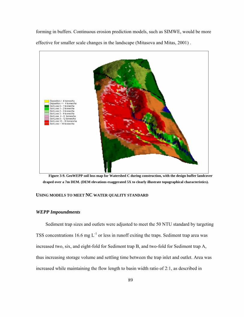
89

forming in buffers. Continuous erosion prediction models, such as SIMWE, would be more

effective for smaller scale changes in the landscape (Mitasova and Mitas, 2001) .

Figure 3-9. GeoWEPP soil loss map for Watershed C during construction, with the design buffer landcover

draped over a 7m DEM. (DEM elevations exaggerated 5X to clearly illustrate topographical characteristics).

USING MODELS TO MEET NC WATER QUALITY STANDARD

WEPP Impoundments

Sediment trap sizes and outlets were adjusted to meet the 50 NTU standard by targeting

TSS concentrations 16.6 mg L-1 or less in runoff exiting the traps. Sediment trap area was

increased two, six, and eight-fold for Sediment trap B, and two-fold for Sediment trap A,

thus increasing storage volume and settling time between the trap inlet and outlet. Area was

increased while maintaining the flow length to basin width ratio of 2:1, as described in

90

NCSCC (1988). The six-fold and eight-fold area simulations of sediment trap B were also

modeled without an outlet to simulate pond hydrology. Culvert outlets with standing pools of

0.46 – 0.76 m were used in place of rock check dams to allow the more sediment laden water

to remain in the trap (Figure 3-10). Culvert inputs were retrieved from default culvert

parameters in WEPP and adjusted to account for sediment trap depth (Table 3-6). This basin

design will be called a “standing pool” hereafter.

NCV - Number of identical culvert outlet structures ACV - Cross-sectional area of culvert (m2) HITCV - Cross-sectional height of culvert (m) for square conduits or diameter for circular conduit HCV - Stage of culvert inlet (m). LCV - Flow length of culvert (m) SCV - Slope of culvert (m/m). HCVOT - Height of culvert outlet above the outlet channel bottom (m)

Figure 3-10. Schematic of culvert impoundment as modeled by WEPP (from Lindley et al., 1998).

91

Table 3-6. WEPP impoundment inputs for sample culvert outlets for sediment traps A & B.

WEPP Impoundment inputs

Culvert parameters

NCV 1

ACV 0.023

HITCV 0.30

HCV

0.46 for Sediment trap A,

0.76 for Sediment trap B

LCV 1.83

SCV 0.01

HCVOT 0.30

Average TSS concentrations and sediment yields in relation to trap size and outlet type

are illustrated in Figure 3-11. Doubling the size of sediment traps A and B had little effect on

sediment yield and runoff volume (Figure 3-11), suggesting that increasing the flow length of

the basin is not an effective method on this site for significantly reducing sediment yield or

runoff. Standing pools with culvert outlets reduced runoff and TSS concentrations in

comparison to the rock check dam outlets (Figure 3-11). Runoff volume for the pool/culvert

design is decreased because runoff remaining in the trap below the culvert outlet exits by

evaporation and infiltration, creating storage for the next storm. TSS concentrations are

reduced because the upper portion of the water column is drained, instead of the entire water

column, as is the case for rock outlets. It should be noted that while culverts do reduce TSS

concentration, the turbidity (550 NTUs, estimated from TSS = 200.5 mg L-1) still far exceeds

the turbidity standard of 50 NTUs. It should also be noted that skimmer outlets are

considered to be far more effective for draining sediment traps than culverts by draining

water consistently from the top portion of the water column (Fennessey and Jarrett, 1997).

Also, skimmers drain the trap until all liquid is removed, allowing for more runoff storage

92

space for the next storm event. Unfortunately skimmer outlets are not modeled by WEPP,

and are in general difficult to model because the outlet position does not remain constant.

Figure 3-11. Predicted average TSS and sediment in outlet directly below sediment trap B during construction.

*Percent of drainage area taken up by the trap.

The N.C. turbidity standard was met when we increased area in trap B 6-fold and 8-fold

and removed the outlet, with turbidity level less than 14 NTUs. When there are no outlets

established for an impoundment in WEPP, runoff exits by overtopping the impoundment.

This was because increasing the area of trap B 6-fold and 8-fold either greatly reduced or

eliminated runoff exiting the trap (Figure 3-11). However, increasing trap area 6-fold would

take up 8 % of the drainage area, and an 8-fold increase would take up 10 % of the drainage

area, which may provide a challenge to most developers.

93

GeoWEPP Vegetation

We attempted to meet the 50 NTU water quality standard in Watershed C by both

adding forest cover to highly erosive areas and by surrounding the entire stream length with a

riparian buffer to prevent sediment from entering the channel. We designed an extended

buffer while maintaining the 15.2 m width set by the original developers, and stretched the

buffer to follow the length of the stream network as delineated by TOPAZ in GeoWEPP.

Forested landcovers for highly erosive areas on the construction site, as detected by

GeoWEPP, were constructed following the method described in Figure 3-6. The landcover

was divided for each scenario as listed in Table 3-7.

Table 3-7. Percent cover of various landcovers in Watershed C.

Landcover No buffer Design buffer Long buffer Long buffer + Low cover

Long buffer + High cover

No construction

Forest and forest buffer 0 11 23 23 23 55

Forested erosion cover 0 0 0 12 32 0

Pavement 1 1 1 1 1 1

Tall grass 21 16 16 16 16 44

Exposed soil surface 78 72 60 48 28 0

Average yearly TSS and sediment yields for various combinations of buffers and

erosive area landcovers are illustrated in Figure 3-12. Extending the design buffer decreased

TSS concentration in comparison to the design buffer by 57 %, and sediment yield by 68 %,

while only increasing vegetation space on the construction site from 13% to 22 %. The large

concentration of yellow raster cells surrounding the channel on the GeoWEPP soil loss map

indicates considerable deposition, thus reducing the amount of sediment reaching the stream

94

(Figure 3-13, Figure 3-14). As mentioned earlier, runoff entering the buffer slows down as a

result of the increased roughness associated with forest landcover, reducing runoff velocities

and increasing deposition. Also providing a vegetative barrier between the exposed soil and

the stream along the length of the stream instead of only the perennial portion (as was

recommended by the developers) prevents direct sediment delivery at the upper half of the

stream. We assumed that the turbidity would far exceed the turbidity standard of 50 NTUs, as

WEPP-predicted TSS concentrations were greater than measured TSS concentrations used to

estimate turbidity using our turbidity-TSS model for this site (Figure 3-5). Overall, extending

the buffer appears to be an effective method for dramatically reducing sediment yields with

minimal use of space, but not effective for meeting water quality standards.

Figure 3-12. Predicted average TSS and sediment in outlet during proposed construction. *Percent of exposed

surface on Watershed C for each landcover scenario.

95

Figure 3-13. Landcover input map for GeoWEPP, simulating a forested buffer extending the length of the

stream on Watershed C during construction.

96

Figure 3-14. GeoWEPP predicted soil loss map, simulating a forested buffer extending the length of the stream

on Watershed C during construction.

GeoWEPP predicted that adding landcover to erosive areas on this site provided little

benefit to reducing sediment yield and TSS (Figure 3-12), which was surprising, as 20 % and

53 % of the previously exposed soil was covered with forest for the low and high cover

scenarios, respectively. This finding may suggest a problem within the GeoWEPP model. It

appears in Figure 3-12 that sediment yield is controlled by runoff volume, and because runoff

volume does not seem to be effected by the addition of cover on erosive areas, then sediment

yield also remains unaffected. In Figure 3-15, Figure 3-16, Figure 3-17, and Figure 3-18,

there appears to be either deposition or soil loss less than 1 tonne ha-1 in the areas of

97

remaining forest, which would be expected, as the increased roughness from bare soil to

forest would reduce runoff and increase deposition.

Figure 3-15. Landcover input map for GeoWEPP, simulating a forested buffer extending the length of the

stream along with forest remaining on moderately erosive areas on Watershed C during construction.

98

Figure 3-16. GeoWEPP predicted soil loss map, simulating a forested buffer extending the length of the stream

along with forest remaining on moderately erosive areas on Watershed C during construction.

99

Figure 3-17. Landcover input map for GeoWEPP, simulating a forested buffer extending the length of the

stream along with forest remaining on highly erosive areas on Watershed C during construction.

100

Figure 3-18. GeoWEPP predicted soil loss map, simulating a forested buffer extending the length of the stream

along with forest remaining on highly erosive areas on Watershed C during construction.

101

Watershed C was modeled under the existing forested conditions to both evaluate

predicted runoff and sediment under pre-construction conditions and to compare to

previously measured runoff and sediment data from that watershed (Figure 3-19). Average

TSS was predicted to be 235.8 mg L-1 (556 NTUs), while the TSS measured in runoff from

Watershed C over 5 storm events averaged at 25.1 mg L-1 (134 NTUs), suggesting that

GeoWEPP is overpredicting sediment concentration in the runoff. This finding is supported

by data generated in Chapter 2, which showed an overestimation of sediment yield on both

Watersheds A and C.

Figure 3-19. Landcover input map for GeoWEPP, simulating a forested cover on Watershed C before

construction.

102

Soil loss was less than 1 tonne ha-1 on shallow slopes in forested areas, and between 1

and 2 tonne ha-1 on steeper slopes and some areas of tall grass (Figure 3-20). These patterns

most likely occurred due to higher runoff velocities on steeper slopes and lower values for

friction factor and interrill cover for tall grass. It should be mentioned that there is not yet an

effective method developed for validating the spatial distribution of erosion on a watershed,

which is why we must use logic and field observations to determine the validity of

GeoWEPP soil loss output maps.

Figure 3-20. GeoWEPP predicted soil loss map, simulating a forested cover on Watershed C before

construction.

103

CONCLUSION

WEPP and GeoWEPP models were applied to determine the efficiency of planned

controls on construction sites and to create BMP scenarios to meet North Carolina water

quality standards. WEPP estimated trapping efficiencies within NC standards of 70 %

trapping efficiency for particle sizes greater than 0.04 mm. WEPP predicted that the runoff

turbidity from the second sediment trap at the site outlet would be equal to or less than NC

turbidity requirements of 50 Nephlometric Turbidity Units for 11 % of storm events. The

GeoWEPP model predicted that planned riparian buffers on Watershed C were not able to

meet the turbidity standard for any of the modeled storm events, and would need to be

combined with other BMPs to decrease the turbidity.

Turbidity standards were met on watershed A by removing the outlet from the second

sediment trap and increasing the trap area 6-fold. Replacing rock check dams with standing

pools with culvert outlets greatly reduced TSS concentrations, although the average turbidity

level of 550 NTUs still exceeded standards. Extending the design buffer decreased TSS

concentration predicted with the design buffer by 57 %, while only increasing vegetation

space on the construction site from 13 % to 22 %. Maintaining forested areas on highly

erosive areas surprisingly had little impact on runoff volume or sediment yield, which may

suggest a potential flaw within the GeoWEPP model.

REFERENCES

Alberts, E. E., M. A. Nearing, M. A. Weltz, L. M. Risse, F. B. Pierson, X. C. Zhang, J. M.

Laflen, and J. R. Simanton. 1995. Chapter 7. Soil component. In: D. C. Flanagan and

104

M. A. Nearing (eds.) 1995. USDA-Water Erosion Prediction project: Hillslope profile

and watershed model documentation. NSERL Report No. 10. USDA-ARS National

Soil Erosion Research Laboratory, West Lafayette, IN 47097-1196.

Doe, W. W., and R. S. Harmon. 2001. Introduction to soil erosion and landscape evolution

modeling. In Landscape Erosion and Evolution Modeling, 1-14. New York, N.Y.:

Kluwer Academic/Plenum Publishers.

Elliot, W. J., and D. E. Hall. 1997. Water Erosion Prediction Project (WEPP) forest

applications. Gen. Tech. Report. INT-GTR-365. Ogden, UT: U.S. Department of

Agriculture, Forest Service, Intermountain Research Station. 11 p.

Fennessey, L. A. J., and A. R. Jarrett. 1997. Influence of principal spillway geometry and

permanent pool depth on sediment retention of sedimentation basins. Trans. ASAE

40(1):53-59.

Flanagan, D. C., and M. A. Nearing (eds.) 1995. USDA-Water Erosion Prediction Project:

WEPP User Summary. NSERL Report No. 10, USDA-ARS National Soil Erosion

Research Laboratory, West Lafayette, Indiana.

Gerwig, B. K., K. C. Stone, R. G. Williams, D. W. Watts, and J. M. Novak. 2001. Using

GLEAMS and REMM to estimate nutrient movement from a spray field and through

a riparian forest. Trans. ASAE 44(3): 505-512.

Goldman, S. J., K. Jackson, and T. Bursztynsky. 1986. Erosion and Sediment Control

Handbook. New York, N.Y.: McGraw-Hill Book Company.

Lienbow, A. M., W. J. Elliot, J. M. Laflen, and K. D. Kohl. 1990. Interrill erodibility:

Collection and analysis of data from cropland soils. Trans. ASAE. 33(6):1882-1888.

105

Lindley, M. R., Barfield, B. J., Ascough II, J. C., Wilson, B. N., and E.W. Stevens. 1998. The

surface impoundment element for WEPP. Trans. ASAE 41(3): 555-564.

Line, D. E., and N. M. White. 2001. Efficiencies of temporary sediment traps on two North

Carolina construction sites. Trans. ASAE. 44(5):1207-1215.

McIsaac, G. F., J. K. Mitchell, J. W. Hummel, and W. J. Elliot. 1992. An evaluation of unit

stream power theory for estimating soil detachment and sediment discharge from

tilled soils. Trans. ASAE. 35(2):535-544.

Mitasova, H., and L. Mitas. 2001. Multiscale soil erosion simulations for land use

management. In Landscape Erosion and Evolution Modeling, 321-347. New York,

N.Y.: Kluwer Academic/Plenum Publishers.

Nearing, M. A., D. I. Page, J. R. Simanton, and L. J. Lane. 1989. Determining erodibility

parameters from rangeland field data for a process-based erosion model. Trans.

ASAE. 32(3):919-924.

North Carolina Sediment Control Commission. 1988. Erosion and sediment control planning

and design manual. Raleigh, NC: Sediment Control Commission.

Neteler, M. and H. Mitasova. 2002. Open Source GIS: A GRASS GIS Approach. Kluwer

Academic Press: Boston, Massachusetts.

Renschler, C. S. 2003. Designing geo-spatial interfaces to scale process models: the

GeoWEPP approach. Hydrol. Process. 17:1005-1017.

SAS. 1999. SAS User's Guide: Statistics. Ver. 8.01. Cary, N.C.: SAS Institute, Inc.

106

Savabi, M. R., W. J. Rawls, and R. W. Knight. 1995a. Water erosion prediction project

(WEPP) rangeland hydrology component evaluation on a Texas range site. J. Range

Mgmt. 48:535-541.

Simanton, J. R., M. A. Weltz, and H. D. Larsen. 1991. Rangeland experiments to paramterize

the water erosion prediction project model: vegetation canopy cover effects. J. Range

Mgmt. 44(3):276-282.

S.C.O.N.C. 2004. State Climate Office of North Carolina. Available at http://www.nc-

climate.ncsu.edu/.

Tomer, M. D., D. E. James, and T. M. Isenhart. 2003. Optimizing the placement of riparian

practices in a watershed using terrain analysis. J. Soil and Water Conserv.58(4): 198-

206.

Toy, T. J, and R. F. Hadley. 1987. Geomorphology and Reclamation of Disturbed Lands. San

Diego, California: Academic Press.

USDA - NRCS. 2000. Soil Survey Geographic (SSURGO) Data. Available at:

http://www.ncgc.nrcs.usda.gov/branch/ssb/products/ssurgo/.

USDA - NRCS. 2002. Official Soil Series Descriptions: Soil Survey Division, Natural

Resources Conservation Service, United States Department of Agriculture. Available

at: http://soils.usda.gov/technical/classification/osd/index.html.

Wilcox, B. P., M. Sbaa, W. H. Blackburn, and J. H. Milligan. 1992. Runoff prediction from

sagebrush rangelands using water erosion prediction project (WEPP) technology. J.

Range Mgmt. 45(5):470-474.

107

Wright, J. A., A. Shirmohammadi, W. L. Magette, J. L. Fouss, R. L. Bengston, and J. E.

Parsons. 1992. Water table management practice effects on water quality. Trans.

ASAE 35(3):823-831.

Yuan, Y., Bingner, R. L., and R. A. Rebich. 2001. Evaluation of AnnAGNPS on Mississippi

Delta MSEA watersheds. Trans. ASAE 44(5):1183-1190.

Zhang, X. C., M. A. Nearing, and L. M. Risse. Estimation of Green-Ampt conductivity

parameters: Part I. Row crops. Trans. ASAE. 38(4):1069-1077.

Zhang, X. C., M. A. Nearing, and L. M. Risse. Estimation of Green-Ampt conductivity

parameters: Part II. Perennial crops. Trans. ASAE. 38(4):1079-1087.

108

APPENDIX

Figure A3-1. Soil grid map at 7 m resolution for watersheds Centennial A (above) and Centennial C (below).

Watersheds are divided into three hillslopes by GeoWEPP.

109

Table A3-1. WEPP watershed characteristics for Centennial watershed.

Left hillslope Top hillslope

Right hillslope Channel

Soil Appling subsoil

Cecil subsoil Cecil Cecil

subsoil Landcover Cutslope Cutslope Forest Cutslope

% Slope 4 10 2 8

Length (m) 94.0 63.4 53.3 72.1

Width (m) 68.7 100.0 68.7 N/A

110

Table A3-2. Rainfall measurements from the RDU airport weather station near Raleigh, NC from 1998 to 1999.

Date Rain (mm) 1/8/98 18.8 1/15/98 53.6 1/18/98 24.9 1/22/98 29.7 1/27/98 47.2 2/3/98 23.4 2/16/98 58.7 2/22/98 11.7 3/8/98 60.5 3/17/98 26.9 3/18/98 98.8 4/4/98 11.1 4/9/98 22.4 5/7/98 21.6 5/11/98 29.0 5/23/98 17.0 6/3/98 20.1 6/15/98 26.7 7/4/98 38.9 7/27/98 20.3 7/30/98 15.7 8/9/98 39.9 8/10/98 11.2 8/16/98 41.2 9/3/98 61.7 9/8/98 12.2 10/4/98 15.2 10/8/98 40.9 11/3/98 24.4 11/4/98 10.9 11/14/98 9.4 11/16/98 12.9 11/26/98 5.6 12/13/98 21.6 12/16/98 17.3 12/24/98 33.0 1/2/99 45.0 1/15/99 10.7 1/18/99 16.0 1/23/99 52.3 2/1/99 14.2 2/17/99 14.2 2/19/99 10.9 3/14/99 40.9 3/21/99 27.9 4/1/99 21.6 4/30/99 42.2 7/13/99 36.1 8/14/99 34.8 8/26/99 21.6 9/4/99 168.2 9/15/99 123.4 9/22/99 15.7 9/27/99 43.7 9/28/99 33.0 9/30/99 19.6 10/17/99 34.8 10/20/99 12.7

111

Date Rain (mm) 11/2/99 8.1 11/26/99 18.3 12/13/99 29.7

112

Table A3-1. Complete list of WEPP landcover input parameters for watersheds A & C on North Carolina State

University's Centennial Campus in Raleigh, North Carolina.

Plant Growth and Harvest Parameters

Cut slope Tall Prairie Grass Disturbed/Forest 20 yr Forest

Biomass energy ratio

(kg MJ-1) 2 13 150 150

Growing degree days to emergence (ºC

day)

30 5 5 5

Growing degree days for growing season (ºC

day)

0 0 0 0

In-row plant spacing (cm) 499.9 10 200 200

Plant stem diameter at

maturity (cm) 0.1 1 25 25

Height of post-harvest

standing residue;

cutting height (cm)

1 10 2000 2000

Harvest index (dry crop yield/total

above ground dry biomass)

(%)

42 42 42 42

Temperature and Radiation

Parameters

Base daily air temperature

(ºC) 2 2 2 2

Optimal temperature

for plant growth (ºC)

12 20 20 20

Maximum temperature

that stops the growth of a

perennial crop (ºC)

32 40 40 40

Critical freezing

temperature for a perennial

crop (ºC)

-40 0 0 0

Radiation extinction coefficient

0.01 0.9 0.9 0.9

Canopy, LAI and Root

Parameters

Canopy cover coefficient 14 14 14 14

113

Plant Growth and Harvest Parameters

Cut slope Tall Prairie Grass Disturbed/Forest 20 yr Forest

Parameter value for

canopy height equation

23 3 3 3

Maximum canopy height

(cm) 15 60 500 500

Maximum leaf area index 1 1 6 6

Maximum root depth (cm) 10 30 200 200

Root to shoot ratio (% root growth / %

above ground growth)

33 33 33 33

Maximum root mass for a

perennial crop (kg/m^2)

0.001 0.15 0.5 0.5

Senescence Parameters

Percent of growing

season when leaf area index

starts to decline

85 25 25 25

Period over which

senescence occurs (days)

14 40 300 300

Percent canopy

remaining after

senescence

0.1 30 50 50

Percent of biomass

remaining after

senescence

1 25 70 70

Residue parameters

Parameter for flat residue

cover equation (m2 kg-1)

5 5 5 5

Standing to flat residue adjustment

factor (wind, snow, etc.) (%)

99 99 99 99

Decomposition constant to

calculate mass change of

above-ground biomass

0.0074 0.0068 0.006 0.006

Decomposition constant to 0.0074 0.0068 0.006 0.006

114

Plant Growth and Harvest Parameters

Cut slope Tall Prairie Grass Disturbed/Forest 20 yr Forest

calculate mass change of root

biomass Use fragile or

non-fragile mfo values

Non-fragile Non-fragile Non-fragile Non-fragile

Other Parameters

Plant specific drought

tolerance (% of soil

porosity)

10 10 10 10

Critical live biomass value below which grazing is not

allowed (kg m-

2)

0 0 0 0

Maximum Darcy

Weisbach friction factor for living plant

1 11 17 17

Harvest Units WeppWillSet WeppWillSet WeppWillSet WeppWillSet Optimal yield under no stress conditions (kg

m-2)

0 0 0 0

Bulk density after tillage (g

cm-3) 1.0 1.1 1.1 1.1

Initial canopy cover (%) 0 30 90 90

Days since last tillage 0 1000 1000 1000

Days since last harvest 0 900 100 100

Initial frost depth (cm) 0 0 0 0

Initial interrill cover (%) 0 80 100 100

Initial residue cropping system

Fallow Perennial Perennial Perennial

Cumulative rainfall since

last tillage (mm)

420.1 1000 1000 1000

Initial ridge height after last tillage

(cm)

0.6 10 10 10

Initial rill cover (%) 0 80 100 100

Initial roughness after last

tillage (cm)

0.6 10 10 10

Rill spacing (cm) 400.1 0 0 0

Rill width type Temporary Temporary Temporary Temporary

115

Plant Growth and Harvest Parameters

Cut slope Tall Prairie Grass Disturbed/Forest 20 yr Forest

Initial snow depth (cm) 0 0 0 0

Initial depth of thaw (cm) 0 0 0 0

Depth of secondary

tillage layer (cm)

2.54 10 10 10

Depth of primary tillage

layer (cm) 2.54 20 20 20

Initial rill width (cm) 0 0 0 0

Initial total dead root mass

(kg m-2) 0 0.1 0.5 0.5

Initial total submerged

residue mass (kg m-2)

0 0.1 0.5 0.5

116

Script A3-1. Newlandcover.aml avenue script for converting raster cells to landcover using soil loss categories; for

this example, we selecteed soil loss categories greater or equal to 6 for designating highly erosive areas on the

landscape. This script was developed by Robert Austin at NC State University.

&args landcov model_cov out_cov &if [null %out_cov%] &then &return &inform Usage new_landcov.aml <landcov> <model_cov> <out_cov> &TYPE &TYPE Starting creation of new landcover.... &TYPE grid /*** Set the size of the analysis environment to the largest extent ***/ setwindow %landcov% setcell %landcov% mapextent %landcov% /*** turn the floating point grid into an integer grid ***/ intgrd = int( %model_cov% ) /*** create a grid with just the 0=not included and 1=included values ***/ selgrid = test( intgrd, 'value <= 10 AND value >= 6' ) /*** fill the nodata values with 0 ***/ bingridfill = con (isnull (selgrid), 0, selgrid) /*** if the boolean grid contains a 1 set it to new class = 10, otherwise keep it the same

***/ %out_cov% = con ( bingridfill == 1, 10, %landcov% ) kill intgrd all kill selgrid all kill bingridfill all &TYPE &TYPE Finised creating %out_cov%.... &TYPE quit &return