ac-514 model based fault-diagnosis for linear systems · teaching affiliation: ... common fault...
TRANSCRIPT

AC-514 Model based Fault-Diagnosis for Linear Systems

Damien Koenig
Research affiliation:
GIPSA-lab, Grenoble Images Speech
Signal and Control, is a joint research
unit of CNRS and University of
Grenoble.
Teaching affiliation:
Grenoble-Inp ESISAR school of
Embedded Systems
My main concerns in automatic control are devoted to state estimation, fault diagnosis and fault tolerant control of complex systems.
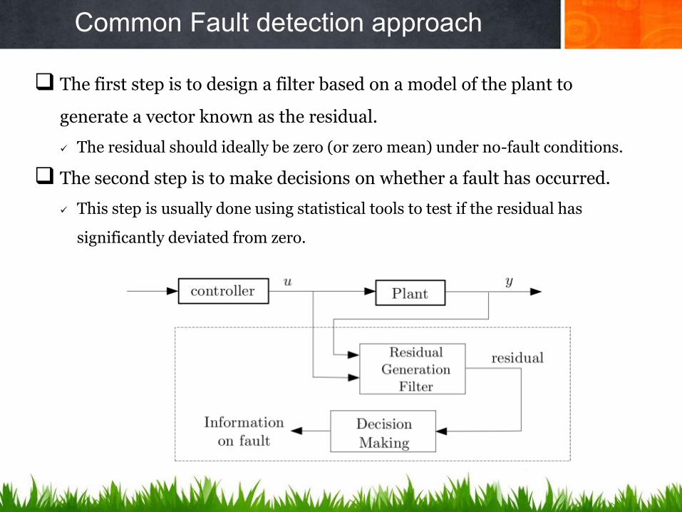
Common Fault detection approach
The first step is to design a filter based on a model of the plant to
generate a vector known as the residual.
The residual should ideally be zero (or zero mean) under no-fault conditions.
The second step is to make decisions on whether a fault has occurred.
This step is usually done using statistical tools to test if the residual has
significantly deviated from zero.

Nomenclature
State and Signals
Fault
An unpermitted deviation of at least one characteristic property or parameter of the system from the acceptable, usual or standard condition.
Failure
A permanent interruption of a system’s ability to perform a required function under specified operating conditions.
Error
A deviation between a measured or computed value of an output variable and its true or theoretically correct one.
Disturbance
An unknown and uncontrolled input acting on a system.
Residual
A fault indicator, based on a deviation between measurements and model-equation-based computations.
Symptom
A change of an observable quantity from normal behavior.

Functions
Fault detection
Determination of faults present in a system and the time of detection
Fault isolation
Determination of the kind, location and time of detection of a fault. Follows fault detection.
Fault identification
Determination of the size and time-variant behavior of a fault. Follows fault isolation
Fault Diagnosis
Determination of the kind, size, location and time of detection of a fault. Follows fault detection. Include Fault detection and identification.
Monitoring
A continuous real-time task of determining the conditions of a physical system, by recording information, recognizing and indication anomalies in the behavior.
Supervision
Monitoring a physical and taking appropriate actions ton maintain the operation in the case of fault.
Nomenclature
Models
Quantitative model
Use of static and dynamic relations among system variables and parameters in order to describe a system’s behavior in quantitative mathematical terms.
Qualitative model
Use of static and dynamic relations among system variables in order to describe a system’s behavior in qualitative terms such as causalities and IF-THEN rules.
Diagnostic model
A set of static or dynamic relations which link specific input variables, to specific output variables, the faults.
Analytical redundancy
Use of more ways to determine a variable, where one way uses mathematical process model in analytical form.
Nomenclature

Models
Reliability (Fiabilité)
Ability of a system to perform a required function under stated conditions, within a given
Safety (Sécurité)
Ability of a system not to cause danger to persons or equipment or the environment.
Availability (disponibilité)
Probability that a system or equipment will operate satisfactorily and effectively at any point of time.
Nomenclature

Time dependency of faults
Abrupt fault
Fault modelled as stepwise function. It represents bias in the monitored signal.
Incipient fault
Fault modelled by using ramp signals. It represents drift (dérive) of the monitored signal.
Intermittent fault
Combination of impulses with different amplitudes.
Nomenclature
Fault terminology
Additive fault
Influence a variable by an addition of the fault itself. They may represent, offsets of sensors.
Multiplicative fault
Are represented by the product of a variable with the fault itself. They can appear as parameter changes within a process.
Nomenclature

Application Examples
Real Processes
FDI applications
DC motor Three tank system Vehicle system

Usual Fault Diagnosis Decomposition
The fault system diagnosis can be decomposed into three parts including
sensors,
actuators,
and system dynamics.
This decomposition is often used in practice. As can be observed from this figure, faults
may occur in any of the three components of the open-loop system as described below.
Furthermore, the plant dynamics and the sensor measurements are always affected by
external system disturbances (or process noises) and measurement noises, respectively.
A reliable fault diagnosis system should be able to distinguish faults from system
disturbances and measurement noise. More precisely, the fault diagnosis system must be
robust to these uncertainties while remaining sensitive to faults.
Sensor faults
Sensors are basically the output interface of a system to the external
world, and convey information about a system’s behavior and its
internal states.
Therefore, sensor faults may cause substantial performance degradation of all
decision-making systems or processes that depend on data integrity for
making decisions.
For example, in a feedback control system, sensors are used either to directly
measure system states or to generate state estimates for the feedback control
law. Thus, the presence of faults in sensors may deteriorate state estimates
and consequently result in inefficient and/or inaccurate control.
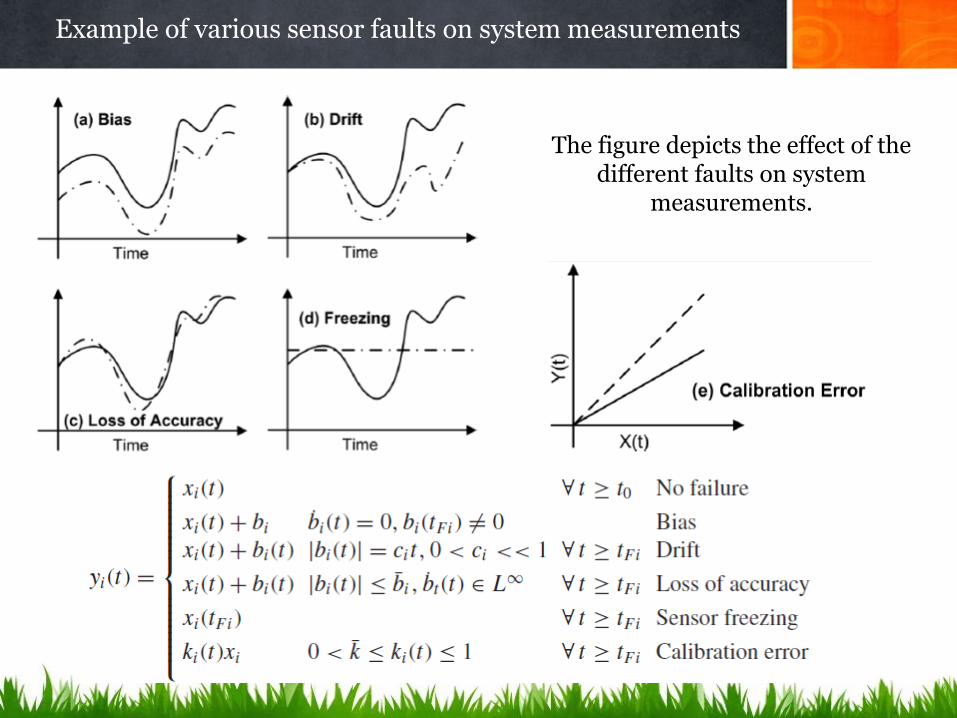
Example of various sensor faults on system measurements
The figure depicts the effect of the different faults on system
measurements.
Actuator faults
In many electromechanical or electrochemical systems, control
signals from the controller (for example, a microprocessor or a
microcontroller) cannot be directly applied to the system. Actuators
are needed to transform control signals to proper actuation signals
such as torques and forces to drive the system.

Common types of actuator faults
For example, common faults in control valve actuators include stuck-open (ouverture coincé), stuck-closed, and abnormal leakage. Another common set of actuator faults especially in servomotors include (a) lock-in-place or freezing; (b) float; (c) hard-over-failure and (d) loss of effectiveness .
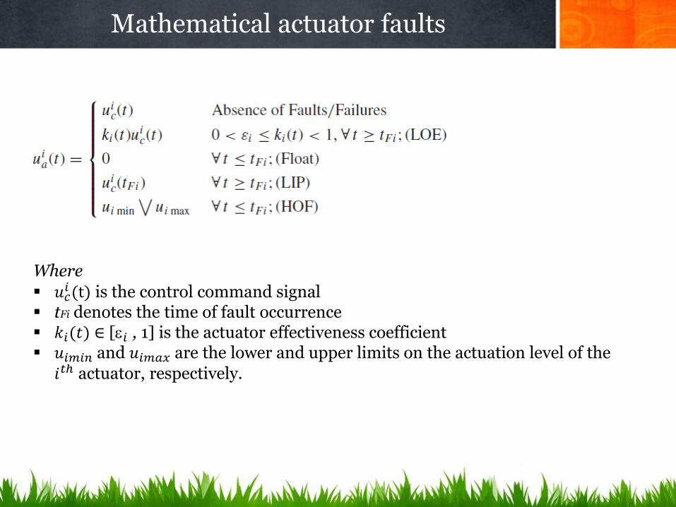
Mathematical actuator faults
Where
𝑢𝑐𝑖 (t) is the control command signal
tFi denotes the time of fault occurrence 𝑘𝑖(𝑡) ∈ [𝑖 , 1] is the actuator effectiveness coefficient 𝑢𝑖𝑚𝑖𝑛 and 𝑢𝑖𝑚𝑎𝑥 are the lower and upper limits on the actuation level of the
𝑖𝑡ℎ actuator, respectively.

Gas Turbine
A gas turbine, also called a combustion turbine, is a type of internal combustion engine. It has an upstream rotating compressor coupled to a downstream turbine, and a combustion chamber in between.
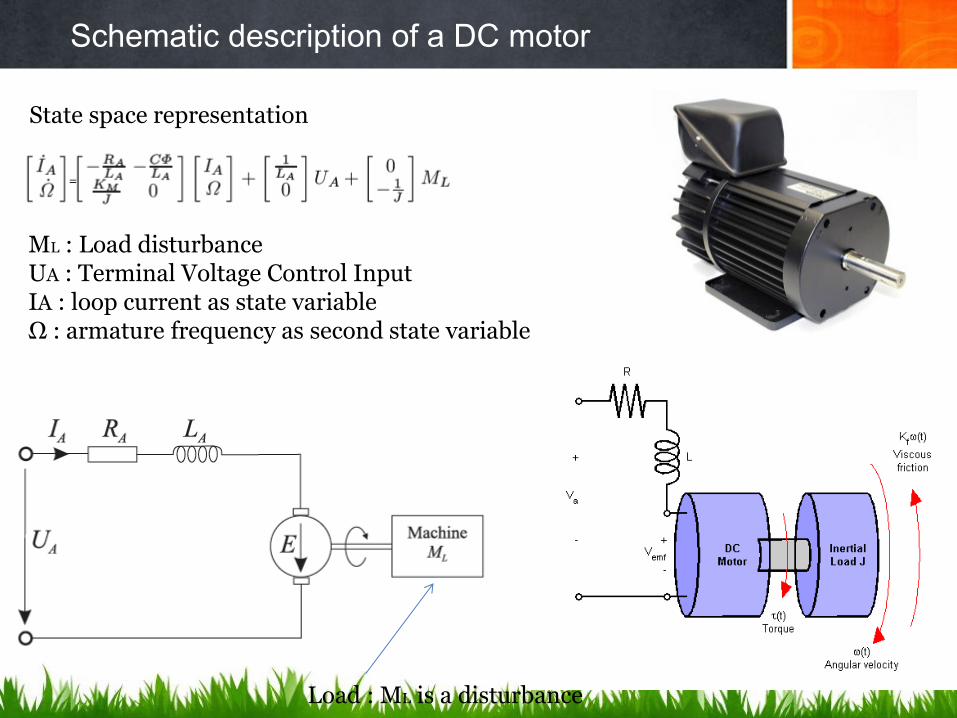
Schematic description of a DC motor
Load : ML is a disturbance
State space representation
=
ML : Load disturbance UA : Terminal Voltage Control Input IA : loop current as state variable Ω : armature frequency as second state variable

Structure of DC motor control system
Load : ML is a disturbance
Plant
y = Ωmeas voltage delivered by the Tacho
For the purpose of speed control, cascade control scheme is adopted with a speed control loop and a current control loop.

Fault diagnosis of DC motor control system
Plant
y = Ωmeas as voltage delivered by the Tacho
Unknown Input
Three faults is considered : • An additive actuator fault fA
• An additive fault sensor fs1
• An multiplicative fault in Tacho fs2
Ωmeas
fS1
fS2
fA

Schematic three tank system
It's typical characteristics of tanks, pipelines and pumps used in chemical industry.

Schematic three tank system
Parameters oh the plant
Linear model at operating point h1=45cm, h2=15cm, and h3 = 30cm

Fault diagnosis of three tank system
Model uncertainty caused by the linearization

Fault diagnosis of three tank system
Modelling of faults Three types of faults are considered :
component faults : leaks in the three tanks, which can be modelled as additional mass flows out of tanks,
where A1, A2 and A3 are unknown and depend on the size of the leaks component faults: plugging between two
tanks sensor faults: three additive faults in the
three sensors, denoted by f1, f2 and f3 actuator faults: faults in pumps, denoted by
f4 and f5
leak
leak

leak
leak
Fault Model diagnosis of three tank
They are modelled as follows
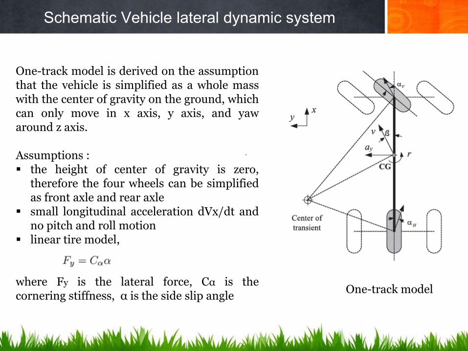
Schematic Vehicle lateral dynamic system
One-track model is derived on the assumption that the vehicle is simplified as a whole mass with the center of gravity on the ground, which can only move in x axis, y axis, and yaw around z axis. Assumptions : the height of center of gravity is zero,
therefore the four wheels can be simplified as front axle and rear axle
small longitudinal acceleration dVx/dt and no pitch and roll motion
linear tire model, where Fy is the lateral force, Cα is the cornering stiffness, α is the side slip angle
One-track model
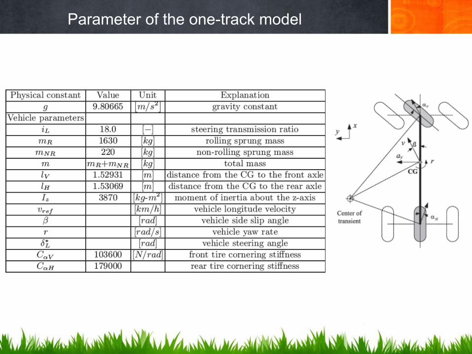
Parameter of the one-track model

Typical sensor noise of vehicle lateral dynamic control systems
In vehicle systems, the variance or standard variance of sensor noises cannot be modelled as constant, since at different driving situations, the sensor noises are not only caused by the sensor own physical or electronic characteristic, but also strongly disturbed by the vibration of vehicle chassis.

Nominal model
The state space presentation of the onetrack model is given by State variables side slip angle β yaw rate r
Typically, a lateral acceleration sensor (ar) and a yaw rate sensor (r) are integrated in vehicles and available, for instance, in ESP (electric stabilization program). The sensor model is given by
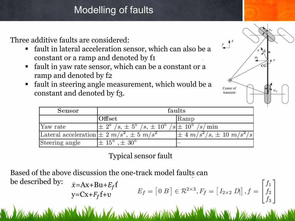
Modelling of faults
Three additive faults are considered: fault in lateral acceleration sensor, which can also be a
constant or a ramp and denoted by f1 fault in yaw rate sensor, which can be a constant or a
ramp and denoted by f2 fault in steering angle measurement, which would be a
constant and denoted by f3.
Based of the above discussion the one-track model faults can be described by:
Typical sensor fault
𝑥 =Ax+Bu+𝐸𝑓f
y=Cx+𝐹𝑓f+υ

Improving the model by including the uncertainties
Vehicle reference velocity vref: the variation of longitudinal vehicle velocity is comparably slow, so it can be considered as a constant during one observation interval.
Vehicle mass: when the load of vehicle varies, accordingly the vehicle spring mass and inertia will be changed. Especially the load variation are very large for the truck, but for the personal car, comparing to large total mass, the change caused by the number of passengers can be neglected normally
Vehicle cornering stiffness Cα: The tire cornering stiffness Cα depends on road-tire, friction coefficient, wheel load, camber(courbure), toe-in(pincement), wheel pressure etc.
is a random number
𝑥 =(A+A)x+(B+B)u+𝐸𝑓f
y=(C+C)x+𝐹𝑓f+υ

Method of Residual Generation
The most relevant analytical model-based residual generation
methods developed have been divided into three categories:
Parity space approach
Observer-based approach
Parameter estimation approach

Model-based FDI Techniques
Residual generation
This block generates residual signals using
available inputs and outputs from the monitored
system. This residual should indicate that a fault
has occurred. It should normally be zero or close
to zero under no fault condition, whilst
distinguishably different from zero when a fault
occurs. This means that the residual is
characteristically independent of process inputs
and outputs, in ideal conditions.

Model-based FDI Techniques
Residual evaluation
This block examines residuals for the likelihood
(probabilité) of faults and a decision rule is then
applied to determine if any faults have occurred.
The residual evaluation block may perform a
simple threshold test on the instantaneous
values or moving averages of the residuals. On
the other hand, it may consist of statistical
methods, e.g., generalized likelihood ratio
testing (assumptions H0, H1).

Modelling of Faulty Systems
Fault diagnosis in a closed-loop system

The controlled system and fault topology
Fault Location:
Actuators
Process or system Components
Input sensors
Output sensors
Controllers
FDI System

Fault and System Modelling
The monitored system and fault topology
State space representation of the plant

Fault and System Modelling
The monitored system and fault topology
State space representation of the plant
Where 𝑒𝑖 is an n-dimensional vector with all zero elements except a 1 in
the 𝑖𝑡ℎ element.
𝑓𝑐 𝑡 = 𝑒𝑖𝑎𝑖𝑗𝑥𝑗(𝑡)

Fault and System Modelling
The monitored system and fault sensor topology
The structure of the plant sensors
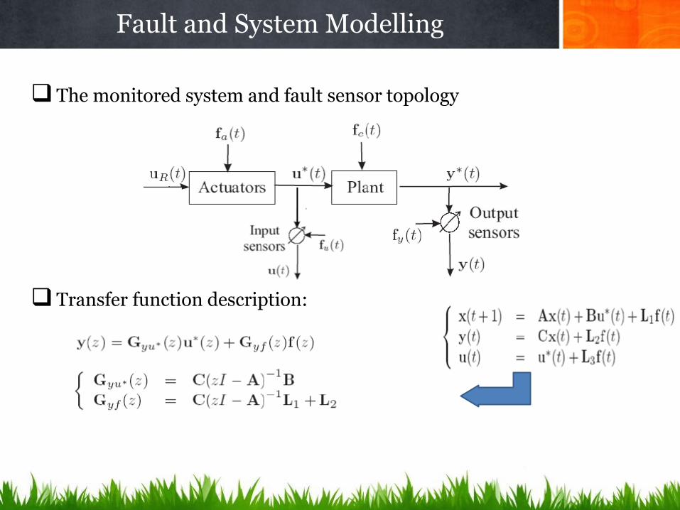
Fault and System Modelling
The monitored system and fault sensor topology
Transfer function description:

Residual Generator Structure
Basic residual generation methods
fault detection filter (FDF)
diagnostic observer (DO)
parity relation based residual generator (PRRG)
parameter estimation
Under fault-free assumptions, the
residual signal r(t) is “almost zero”
Residual Generator Structure
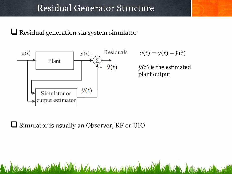
Residual generation via system simulator
Simulator is usually an Observer, KF or UIO
𝑟 𝑡 = 𝑦 𝑡 − 𝑦 (𝑡)
𝑦 (𝑡) is the estimated plant output

Residual Generator Structure
Residual generator:
Constraint conditions: design
𝑟 𝑧 = 𝐻𝑢∗ 𝑧 𝑢∗(z)+𝐻𝑦 𝑧 𝑦 (z)
r(t)=0 if and only if f(t) = 0
y 𝑧 = 𝐺𝑦𝑓 𝑧 𝑓(z)+𝐺𝑦𝑢∗ 𝑧 𝑢∗(z)
𝐻𝑢∗ 𝑧 + 𝐻𝑦 𝑧 𝐺𝑦𝑢∗ 𝑧 =0
𝐻𝑦 𝑧 𝐺𝑦𝑓 𝑧 ≠0
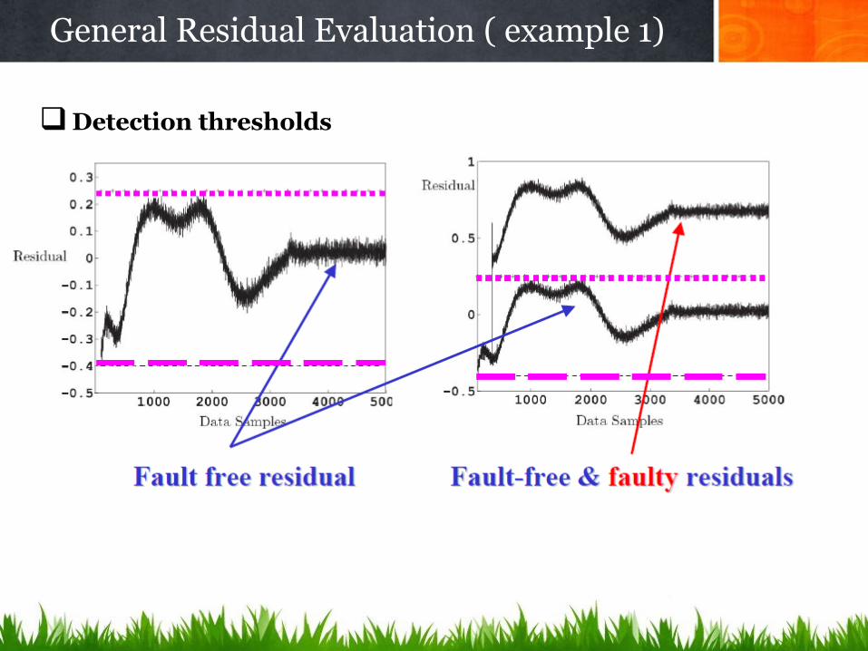
General Residual Evaluation ( example 1)
Detection thresholds
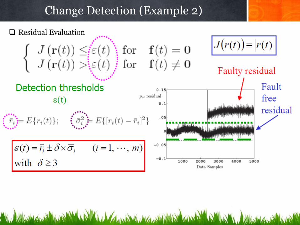
Change Detection (Example 2)
Residual Evaluation

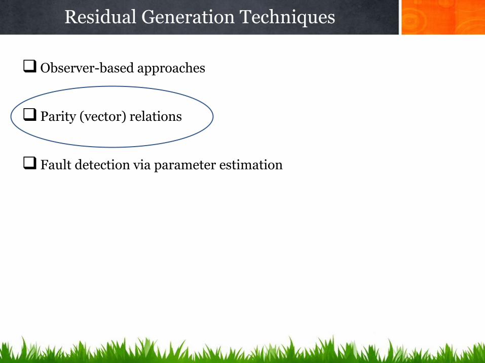
Observer-based approaches
Parity (vector) relations
Fault detection via parameter estimation
Residual Generation Techniques
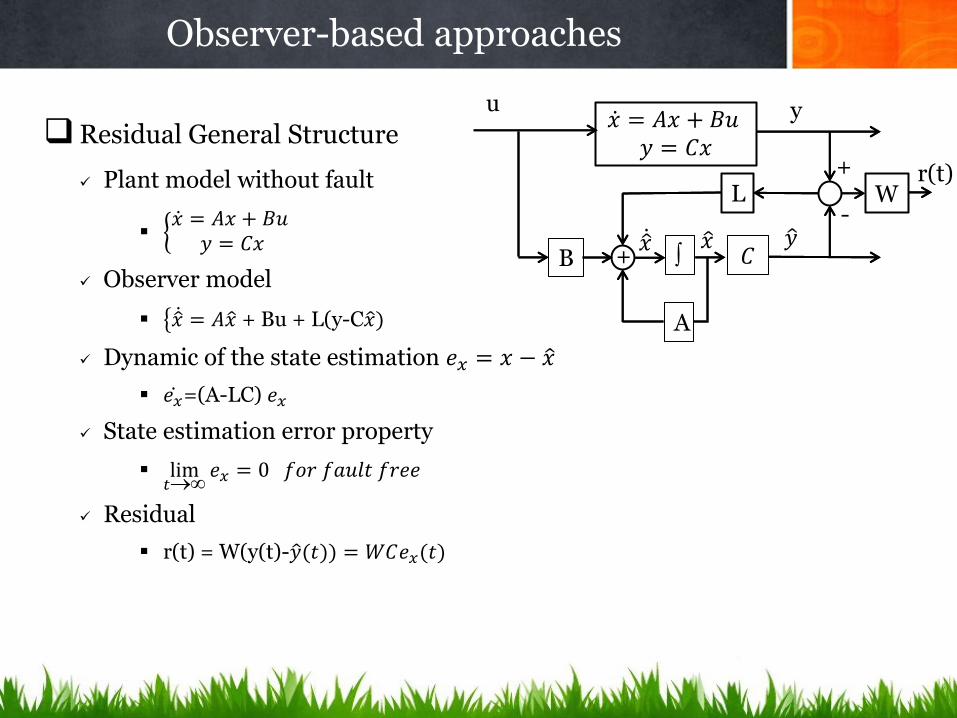
Residual General Structure
Plant model without fault
𝑥 = 𝐴𝑥 + 𝐵𝑢
𝑦 = 𝐶𝑥
Observer model
𝑥 = 𝐴𝑥 + Bu + L(y-C𝑥 )
Dynamic of the state estimation 𝑒𝑥 = 𝑥 − 𝑥
𝑒𝑥 =(A-LC) 𝑒𝑥
State estimation error property
lim𝑡
𝑒𝑥 = 0 𝑓𝑜𝑟 𝑓𝑎𝑢𝑙𝑡 𝑓𝑟𝑒𝑒
Residual
r(t) = W(y(t)-𝑦 (𝑡)) = 𝑊𝐶𝑒𝑥(𝑡)
Observer-based approaches
B
u
𝑥
𝐶
y
𝑥
A
𝑦
𝑥 = 𝐴𝑥 + 𝐵𝑢 𝑦 = 𝐶𝑥
W r(t)
L
+
+
-

Residual General Structure
Plant model with fault
𝑥 = 𝐴𝑥 + 𝐵𝑢+𝐹𝑥f
𝑦 = 𝐶𝑥 + 𝐹𝑠f
Observer model
𝑥 = 𝐴𝑥 + Bu+L(y−C𝑥 )
𝑦 = 𝐶𝑥
Dynamic of the state estimation 𝑒𝑥 = 𝑥 − 𝑥
𝑒𝑥 =(A-LC) 𝑒𝑥+ 𝐹𝑥f −L𝐹𝑠f
Output state estimation error
𝑦 (t)=y(t)-𝑦 (𝑡)=C𝑒𝑥 𝑡 + 𝐹𝑠f(t)
State estimation error property
lim𝑡
𝑒𝑥 ≠ 0 𝑤ℎ𝑒𝑛 𝑎 𝑓𝑎𝑢𝑙𝑡 𝑜𝑐𝑐𝑢𝑟
Residual
r(t) = W(y(t)-𝑦 (𝑡)) = 𝑊𝐶𝑒𝑥(𝑡)+W𝐹𝑠f(t)
lim𝑡
𝑟 𝑡 = −𝑊𝐶 𝐴 − 𝐿𝐶 −1(𝐹𝑥 − 𝐿𝐹𝑠)+W𝐹𝑠 𝑓(𝑡) ≠ 0 𝑤ℎ𝑒𝑛 𝑎 𝑓𝑎𝑢𝑙𝑡 𝑜𝑐𝑐𝑢𝑟
Observer-based approaches
B
u
𝑥
𝐶
y
𝑥
A
𝑦
𝑥 = 𝐴𝑥 + 𝐵𝑢∗
𝑦∗ = 𝐶𝑥
W r(t)
L
+
+
-
𝐹𝑥
f
𝐹𝑦
𝑢∗ 𝑦∗

In order to describe the BFDF, the simple fault model is used
𝑥 = 𝐴𝑥 + 𝐵𝑢+𝑏𝑖𝑓𝑎𝑖(𝑡)
𝑦 = 𝐶𝑥 + 𝐼𝑗𝑓𝑠𝑗(𝑡)
Where
𝑏𝑖𝑓𝑎𝑖(𝑡) (i=1,2, …, r) denotes that a fault occurred in the 𝑖𝑡ℎ 𝑎𝑐𝑡𝑢𝑎𝑡𝑜𝑟, 𝑏𝑖 ∈ 𝑅𝑛 is the 𝑖𝑡ℎ column of the input matrix B and 𝑓𝑎𝑖(𝑡) is an unknown scalar time-varying function which represents the evolution of the fault.
𝐼𝑗𝑓𝑠𝑗(𝑡) (j=1,2, …, m) denotes that a fault occurs in the 𝑗𝑡ℎ 𝑠𝑒𝑛𝑠𝑜𝑟, 𝐼𝑗 ∈ 𝑅𝑚 is a unit vector corresponding to a fault occurs in the 𝑗𝑡ℎ 𝑠𝑒𝑛𝑠𝑜𝑟.
BFDF
𝑥 = 𝐴𝑥 + Bu + L(y-C𝑥 )
State estimation error property
𝑒𝑥 =(A-LC) 𝑒𝑥+𝑏𝑖𝑓𝑎𝑖(𝑡)−L𝐼𝑗𝑓𝑠𝑗(𝑡)
Output state estimation error
𝑦 (t)=C𝑒𝑥 𝑡 + 𝐼𝑗𝑓𝑠𝑗(𝑡)
Residual
lim𝑡
𝑟 𝑡 ≠ 0 𝑤ℎ𝑒𝑛 𝑓𝑎𝑢𝑙𝑡 𝑠𝑒𝑛𝑠𝑜𝑟 𝑜𝑟 𝑎𝑐𝑡𝑢𝑎𝑡𝑜𝑟 𝑜𝑐𝑐𝑢𝑟
Basic principles of fault detection filters (BFDF)

The sensor fault model is described by
𝑥 = 𝐴𝑥 + 𝐵𝑢 𝑦 = 𝐶𝑥 + 𝑓𝑠(𝑡)
Where
𝑓𝑠 𝑡 denotes the faults sensor vector
We build a bank of Observers, where each
observer i is piloted by sensor 𝑦𝑖
𝑥 = 𝐴𝑥 + Bu + 𝐿𝑖(𝑦𝑖 -𝐶𝑖𝑥 )
State estimation error property
𝑒𝑥 =(A-𝐿𝑖𝐶𝑖) 𝑒𝑥−𝐿𝑖𝑓𝑠𝑖(𝑡)
Output state estimation error
𝑟𝑖(t)=𝑦𝑖-𝑦𝑖 = 𝐶𝑖 𝑒𝑥 𝑡 + 𝑓𝑠𝑖(𝑡)
Residual
lim𝑡
𝑟𝑖 𝑡 ≠ 0 𝑤ℎ𝑒𝑛 𝑓𝑠𝑖(𝑡) hold true
𝑟𝑖 𝑡
Case 1 : Simultaneous faults sensor
𝑥 = 𝐴𝑥 + 𝐵𝑢
𝑦𝑖 = 𝐶𝑖𝑥 + 𝑓𝑠𝑖(𝑡)
𝑖𝑡ℎ sensor fault model
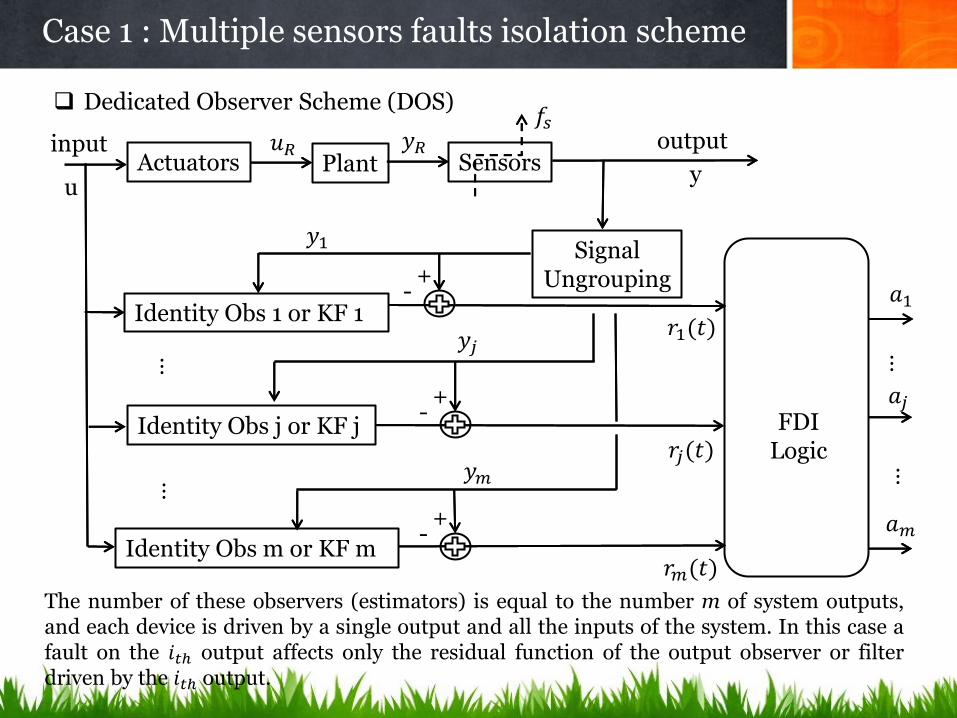
Case 1 : Multiple sensors faults isolation scheme
u
input Actuators Plant Sensors
𝑢𝑅 𝑦𝑅
y
Identity Obs 1 or KF 1
⋮
⋮
Signal Ungrouping
𝑦1
output
FDI Logic
𝑟1(𝑡) 𝑦𝑗
Identity Obs j or KF j
Identity Obs m or KF m
𝑦𝑚 𝑟𝑗(𝑡)
𝑟𝑚(𝑡)
Dedicated Observer Scheme (DOS)
The number of these observers (estimators) is equal to the number m of system outputs, and each device is driven by a single output and all the inputs of the system. In this case a fault on the 𝑖𝑡ℎ output affects only the residual function of the output observer or filter driven by the 𝑖𝑡ℎ output.
𝑓𝑠
⋮
⋮
𝑎1
𝑎𝑗
𝑎𝑚
+ -
+ -
+ -

A simple threshold logic can be used to make decision about the
appearance of a specific fault by the logic decision according to:
‖ 𝑟𝑖 (t)‖≥ 𝑖 implies 𝑓𝑠𝑖≠0
This isolable residual structure is very simple and all faults can be
detected simultaneously, however it is difficult to design in practice.
Case 1 : A simple threshold logic for DOS
𝒓𝟏 𝒓𝟐 … 𝒓𝒎
𝑓𝑠1 1 0 … 0
𝑓𝑠2 0 1 0
⋮ ⋱ 0
𝑓𝑠𝑚 0 0 1
Table 2 : DOS
In the tables above, a "1" in 𝑖𝑡ℎ row and 𝑖𝑡ℎ column denotes that the residual 𝑟𝑖 is sensitive to the fault 𝑓𝑠𝑖, whilst a "0" denotes insensitivity.
𝑎1=1 if 𝑓𝑠1 hold true
𝑎𝑚=1 if 𝑓𝑠𝑚 hold true
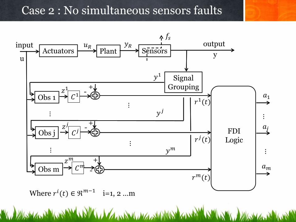
Case 2 : No simultaneous sensors faults
u
input Actuators Plant Sensors
𝑢𝑅 𝑦𝑅
y
Obs 1
Obs j
Obs m
⋮
⋮
Signal Grouping
𝑦1
output
FDI Logic
𝑟1(𝑡)
𝑦𝑗
𝑦𝑚
+
+
+
𝑟𝑗(𝑡)
𝑟𝑚(𝑡)
- 𝐶1
𝑧1
- 𝐶𝑗
𝑧𝑗
- 𝐶𝑚 𝑧𝑚
⋮
⋮
Where 𝑟𝑖(𝑡) ∈ 𝑚−1 i=1, 2 …m
𝑓𝑠
⋮
⋮
𝑎1
𝑎𝑗
𝑎𝑚
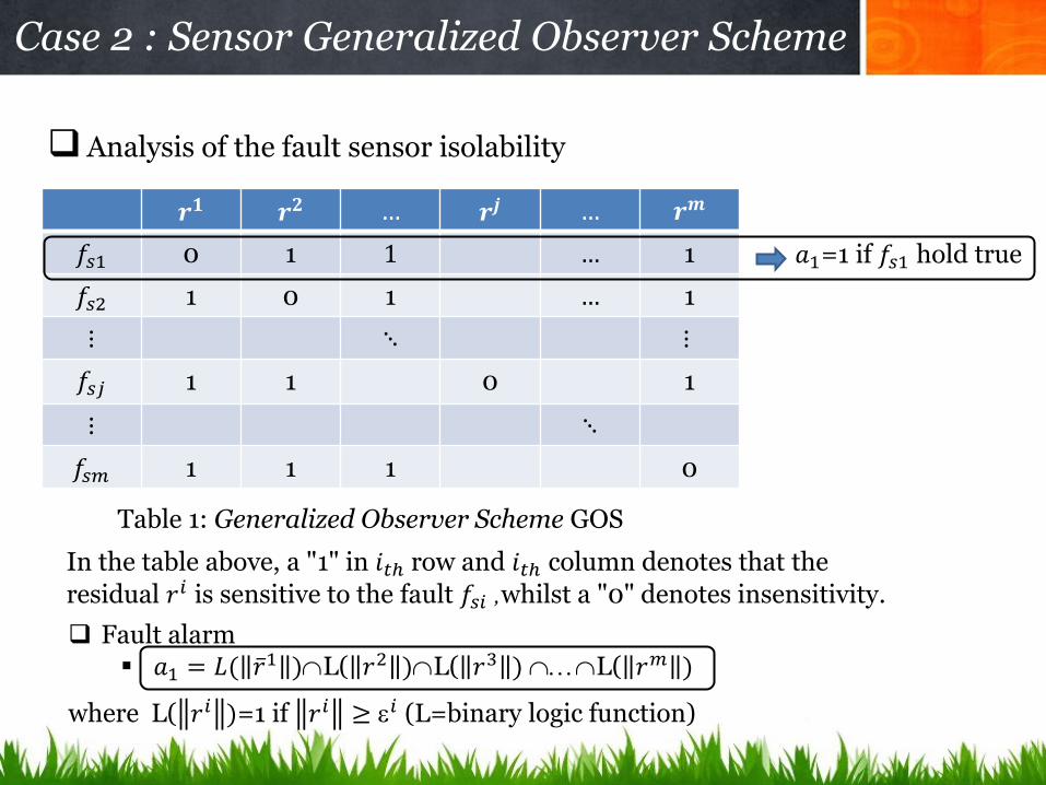
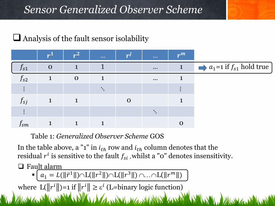
Analysis of the fault sensor isolability
Case 2 : Sensor Generalized Observer Scheme
𝒓𝟏 𝒓𝟐 … 𝒓𝒋 … 𝒓𝒎
𝑓𝑠1 0 1 1 … 1
𝑓𝑠2 1 0 1 … 1
⋮ ⋱ ⋮
𝑓𝑠𝑗 1 1 0 1
⋮ ⋱
𝑓𝑠𝑚 1 1 1 0
Table 1: Generalized Observer Scheme GOS
In the table above, a "1" in 𝑖𝑡ℎ row and 𝑖𝑡ℎ column denotes that the
residual 𝑟𝑖 is sensitive to the fault 𝑓𝑠𝑖 ,whilst a "0" denotes insensitivity.
Fault alarm 𝑎1 = 𝐿( 𝑟 1 )L( 𝑟2 )L( 𝑟3 ) L( 𝑟𝑚 )
where L( 𝑟𝑖 )=1 if 𝑟𝑖 ≥ 𝑖 (L=binary logic function)
𝑎1=1 if 𝑓𝑠1 hold true

The main task of robust FDI is to generate a residual signal which is robust to
the system uncertainty.
According to the previous discussion, a system with possible sensor and actuator
faults can be described as :
𝑥 = 𝐴𝑥 + 𝐵𝑢+𝐸𝑑 𝑡 + 𝐵𝑓𝑎(𝑡)
𝑦 = 𝐶𝑥 + 𝑓𝑠 (𝑡)
Where
𝑓𝑎(𝑡) 𝑟 is the actuator faults
𝑓𝑠(𝑡) 𝑚 is the sensor faults
𝑑𝑞 is the unknown input (or disturbance)
To generate a robust residual an UIO is designed :
𝑧 (𝑡) = 𝐹𝑧(𝑡) + 𝑇𝐵𝑢(t)+𝐺𝑦(𝑡)
𝑥 (𝑡) = 𝑧(𝑡) + 𝑁𝑦(𝑡)
Where 𝑥 𝑛 is the estimated state vector and z𝑛 is the state of the full order
observer, and F, T G, N are matrices to be designed for achieving unknown input de-
coupling and other design requirements.
Residual
r(t)=y(t)-C𝑥 (𝑡)
Robust FDI schemes based on UIOs

When the UIO-based residual is applied to the previous system, the residual and state
estimation errors become:
𝑒𝑥(𝑡) = 𝑥(𝑡) − 𝑥 𝑡 =(I-NC)x- 𝑧 𝑡 − 𝑁𝑓𝑠 𝑡 = Tx(t) − z(t) − N 𝑓𝑠 𝑡
r(t)=y(t)-C𝑥 𝑡 = 𝐶𝑒𝑥 + 𝑓𝑠 (𝑡)
Where T=I-NC
Dynamic of the state estimation error
𝑒 𝑥 = T𝑥 t − 𝑧 t − N𝑓𝑠 𝑡 = 𝑇𝐴 − 𝐺𝐶 𝑥+T𝐸𝑑 𝑡 + 𝑇𝐵𝑓𝑎 𝑡 − 𝐹𝑧 𝑡 − 𝐺𝑓𝑠 𝑡 − N𝑓𝑠 𝑡
𝑒 𝑥= 𝑇𝐴 − 𝐺𝐶 𝑥+T𝐸𝑑 𝑡 + 𝑇𝐵𝑓𝑎 𝑡 − 𝐹(Tx(t) − N 𝑓𝑠 𝑡 − 𝑒𝑥) − 𝐺𝑓𝑠 𝑡 − N𝑓𝑠 𝑡
𝑒 𝑥= F 𝑒𝑥 + 𝑇𝐴 − 𝐺𝐶 − 𝐹𝑇 𝑥+T𝐸𝑑 𝑡 + 𝑇𝐵𝑓𝑎 𝑡 + (𝐹N −G)𝑓𝑠 𝑡 − N𝑓𝑠 𝑡
If one can make the following relations hold true
𝑇𝐴 − 𝐺𝐶 − 𝐹𝑇=0
T=I-NC
K= -(𝐹N−G)=G−FN
TE=0
The state estimation error will then be:
𝑒 𝑥= F 𝑒𝑥 + 𝑇𝐵𝑓𝑎 𝑡 − 𝐾𝑓𝑠 𝑡 − N𝑓𝑠 𝑡
If all eigenvalues of F are stable, then
lim𝑡
𝑟 𝑡 < Threshold for fault free case
lim𝑡
𝑟 𝑡 ≥ Threshold for faulty case
UIO observer design

1) Check the UI decoupled condition
Rank(CE)=Rank(E)=dim(d)
2) Compute
TE=0 (I-NC)E=0 E=NCE N=E(CE)+=E (𝐶𝐸)(𝐶𝐸)𝑇 −1(𝐶𝐸)𝑇 Deduce N and T=I-NC
3) Solve the Syvester equation
𝑇𝐴 − 𝐺𝐶 − 𝐹𝑇=0 TA-GC-F(I-NC)=0F=TA-(G-FN)C F=TA-KC Check the observabilty (or detectability) of the pair(TA, C), if (TA, C) observable
(detectable), a UIO exists and K can be computed using pole placement or LQ method. Deduce K, F, G=K+FN
The UIO-based residual is also reduced to:
𝑒 𝑥= F 𝑒𝑥 + 𝑇𝐵𝑓𝑎 𝑡 − 𝐾𝑓𝑠 𝑡 − N𝑓𝑠 𝑡 r(t)=𝐶𝑒𝑥 + 𝑓𝑠 (𝑡)
It can be seen that the disturbance effects have been de-coupled from the residual.
To detect actuator faults, one has to make:
TB≠0
More specifically, the fault in the 𝑖𝑡ℎ actuator will affect the residual iff:
T𝑏𝑖≠0
Where 𝑏𝑖 is the 𝑖𝑡ℎ column of the matrix B.
UIO design procedure
The fault isolation problem is to located the fault, i.e., to determine
in which sensor (or actuator) fault has occurred.
The sensitivity and insensitivity properties makes isolation possible.
The ideal situation is to make each residual only sensitive to a
particular fault and insensitive to all other faults. However, this ideal
situation is normally difficult to achieve.
Robust fault isolation schemes based on UIOs
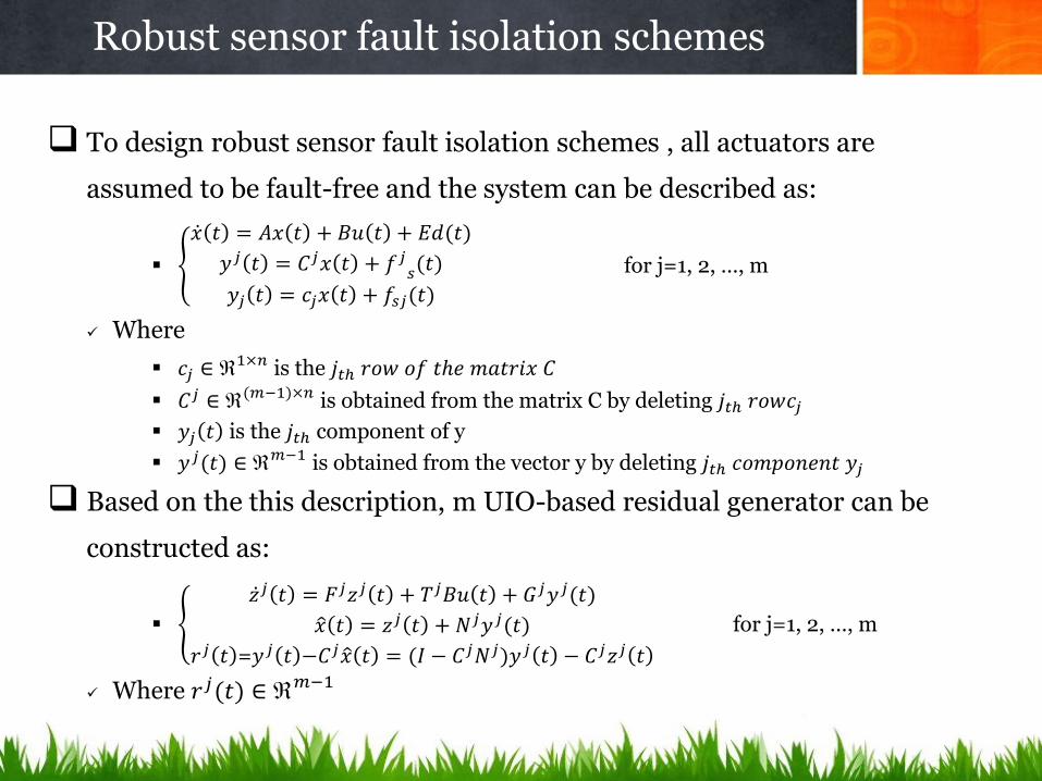
To design robust sensor fault isolation schemes , all actuators are
assumed to be fault-free and the system can be described as:
𝑥 𝑡 = 𝐴𝑥 𝑡 + 𝐵𝑢 𝑡 + 𝐸𝑑(𝑡)
𝑦𝑗 𝑡 = 𝐶𝑗𝑥 𝑡 + 𝑓𝑗𝑠(𝑡)
𝑦𝑗 𝑡 = 𝑐𝑗𝑥 𝑡 + 𝑓𝑠𝑗(𝑡)
for j=1, 2, …, m
Where
𝑐𝑗 ∈ 1×𝑛 is the 𝑗𝑡ℎ 𝑟𝑜𝑤 𝑜𝑓 𝑡ℎ𝑒 𝑚𝑎𝑡𝑟𝑖𝑥 𝐶
𝐶𝑗 ∈ (𝑚−1)×𝑛 is obtained from the matrix C by deleting 𝑗𝑡ℎ 𝑟𝑜𝑤𝑐𝑗
𝑦𝑗 𝑡 is the 𝑗𝑡ℎ component of y
𝑦𝑗(𝑡) ∈ 𝑚−1 is obtained from the vector y by deleting 𝑗𝑡ℎ 𝑐𝑜𝑚𝑝𝑜𝑛𝑒𝑛𝑡 𝑦𝑗
Based on the this description, m UIO-based residual generator can be
constructed as:
𝑧 𝑗 𝑡 = 𝐹𝑗𝑧𝑗 𝑡 + 𝑇𝑗𝐵𝑢 𝑡 + 𝐺𝑗𝑦𝑗(𝑡)
𝑥 𝑡 = 𝑧𝑗 𝑡 + 𝑁𝑗𝑦𝑗(𝑡)
𝑟𝑗 𝑡 =𝑦𝑗 𝑡 −𝐶𝑗𝑥 𝑡 = (𝐼 − 𝐶𝑗𝑁𝑗)𝑦𝑗 𝑡 − 𝐶𝑗𝑧𝑗 𝑡
for j=1, 2, …, m
Where 𝑟𝑗(𝑡) ∈ 𝑚−1
Robust sensor fault isolation schemes

In order to obtain an UIO, the parameter matrices must satisfy the
following equalities:
𝑁𝑗 =E(𝐶𝑗E)+=E (𝐶𝑗𝐸)(𝐶𝑗𝐸)𝑇 −1(𝐶𝑗𝐸)𝑇
𝑇𝑗=I- 𝑁𝑗 𝐶𝑗
𝐹𝑗=𝑇𝑗A- 𝐾𝑗 𝐶𝑗 to be stabilized
𝐺𝑗 = 𝐾𝑗 +𝐹𝑗𝑁𝑗
for j=1, 2, …, m
When all actuators are fault free and a fault occurs in the 𝑗𝑡ℎ sensor,
the residual will satisfy the following isolation logic:
𝑟𝑗(𝑡) < 𝑗
𝑟𝑘(𝑡) ≥ 𝑘 for k=1, …, j-1, j+1, …,m
Where 𝑗 (j=1, 2…,m) are isolation threshold.
Robust sensor fault isolation schemes

A robust sensor fault isolation scheme
u
input Actuators Plant Sensors
𝑢𝑅 𝑦𝑅
y
UIO 1
UIO j
UIO m
⋮
⋮
(𝐼 − 𝐶1𝑁1) Signal
Grouping
𝑦1
output
FDI Logic
𝑟1(𝑡)
(𝐼 − 𝐶𝑗𝑁𝑗)
(𝐼 − 𝐶𝑚𝑁𝑚)
𝑦𝑗
𝑦𝑚
+
+
+
𝑟𝑗(𝑡)
𝑟𝑚(𝑡)
- 𝐶1
𝑧1
- 𝐶𝑗
𝑧𝑗
- 𝐶𝑚 𝑧𝑚
⋮
⋮
Where 𝑟𝑖(𝑡) ∈ 𝑚−1 i=1, 2 …m
𝑓𝑠
⋮
⋮
𝑎1
𝑎𝑗
𝑎𝑚
Analysis of the fault sensor isolability
Sensor Generalized Observer Scheme
𝒓𝟏 𝒓𝟐 … 𝒓𝒋 … 𝒓𝒎
𝑓𝑠1 0 1 1 … 1
𝑓𝑠2 1 0 1 … 1
⋮ ⋱ ⋮
𝑓𝑠𝑗 1 1 0 1
⋮ ⋱
𝑓𝑠𝑚 1 1 1 0
Table 1: Generalized Observer Scheme GOS
In the table above, a "1" in 𝑖𝑡ℎ row and 𝑖𝑡ℎ column denotes that the
residual 𝑟𝑖 is sensitive to the fault 𝑓𝑠𝑖 ,whilst a "0" denotes insensitivity.
Fault alarm 𝑎1 = 𝐿( 𝑟 1 )L( 𝑟2 )L( 𝑟3 ) L( 𝑟𝑚 )
where L( 𝑟𝑖 )=1 if 𝑟𝑖 ≥ 𝑖 (L=binary logic function)
𝑎1=1 if 𝑓𝑠1 hold true

Existence condition : In order to satisfy the constraints
𝑇𝑗E=0 𝑐1 : decoupled condition
𝐹𝑗=𝑇𝑗A- 𝐾𝑗 𝐶𝑗 stable 𝑐2 : detectability condition
the following rank conditions must be verified for each observer :
𝑐1: rank 𝐶𝑗 E𝐸
=rank 𝐶𝑗 E =dim(d)
𝑐2: rank 𝑝𝐼𝑛 − 𝑇𝑗𝐴
𝐶𝑗=n ((𝑇𝑗𝐴))≥0
Proof of 𝑐1 : 𝑇𝑗 E=0 (I- 𝑁𝑗 𝐶𝑗 )E=0 𝑁𝑗 𝐶𝑗 E=E
The solution of 𝑁𝑗 𝐶𝑗 E=E depends on the rank of matrix 𝐶𝑗 E.
A solution exists iff : rank 𝐶𝑗 E𝐸
=rank 𝐶𝑗 E =dim(d) [Rao]
C. R. Rao and S. K. Mitra, Generalized Inverse of Matrices and Its Applications. New York: Wiley, 1971.
Robust sensor fault isolation schemes
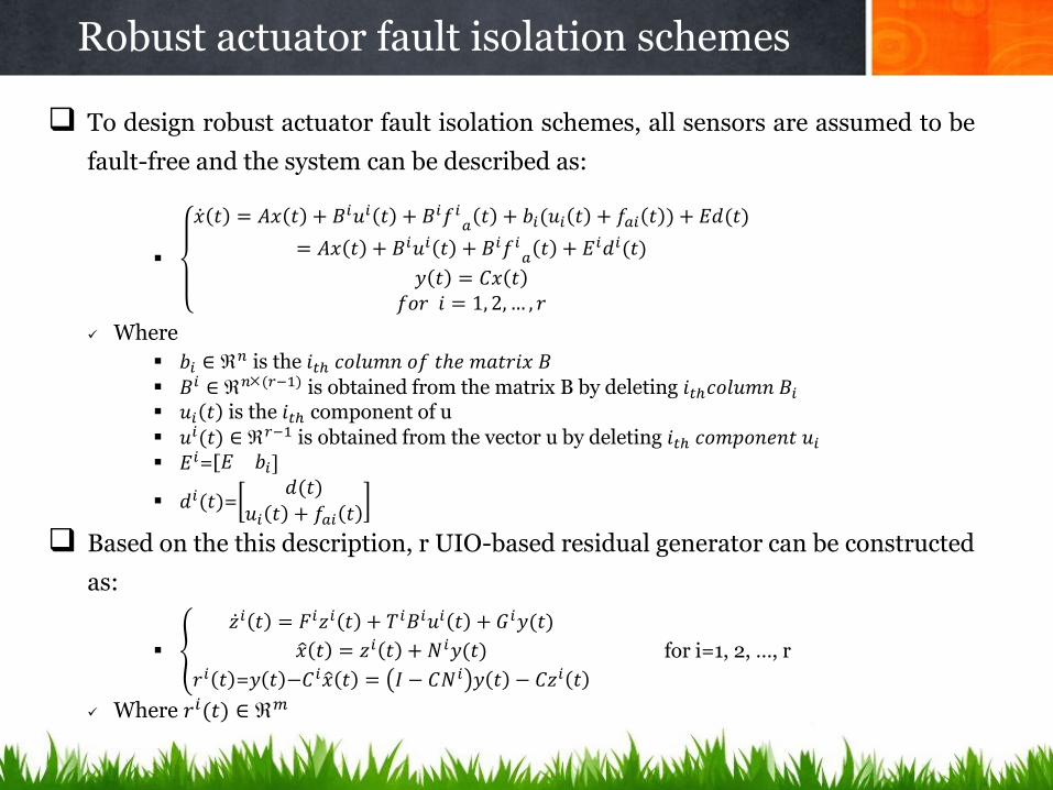
To design robust actuator fault isolation schemes, all sensors are assumed to be
fault-free and the system can be described as:
𝑥 𝑡 = 𝐴𝑥 𝑡 + 𝐵𝑖𝑢𝑖 𝑡 + 𝐵𝑖𝑓𝑖𝑎
𝑡 + 𝑏𝑖(𝑢𝑖 𝑡 + 𝑓𝑎𝑖 𝑡 ) + 𝐸𝑑(𝑡)
= 𝐴𝑥 𝑡 + 𝐵𝑖𝑢𝑖 𝑡 + 𝐵𝑖𝑓𝑖𝑎
𝑡 + 𝐸𝑖𝑑𝑖(𝑡)
𝑦 𝑡 = 𝐶𝑥 𝑡𝑓𝑜𝑟 𝑖 = 1, 2, … , 𝑟
Where
𝑏𝑖 ∈ 𝑛 is the 𝑖𝑡ℎ 𝑐𝑜𝑙𝑢𝑚𝑛 𝑜𝑓 𝑡ℎ𝑒 𝑚𝑎𝑡𝑟𝑖𝑥 𝐵
𝐵𝑖 ∈ 𝑛(𝑟−1) is obtained from the matrix B by deleting 𝑖𝑡ℎ𝑐𝑜𝑙𝑢𝑚𝑛 𝐵𝑖 𝑢𝑖 𝑡 is the 𝑖𝑡ℎ component of u
𝑢𝑖(𝑡) ∈ 𝑟−1 is obtained from the vector u by deleting 𝑖𝑡ℎ 𝑐𝑜𝑚𝑝𝑜𝑛𝑒𝑛𝑡 𝑢𝑖
𝐸𝑖=[𝐸 𝑏𝑖]
𝑑𝑖(𝑡)=𝑑(𝑡)
𝑢𝑖 𝑡 + 𝑓𝑎𝑖 𝑡
Based on the this description, r UIO-based residual generator can be constructed
as:
𝑧 𝑖 𝑡 = 𝐹𝑖𝑧𝑖 𝑡 + 𝑇𝑖𝐵𝑖𝑢𝑖 𝑡 + 𝐺𝑖𝑦(𝑡)
𝑥 𝑡 = 𝑧𝑖 𝑡 + 𝑁𝑖𝑦(𝑡)
𝑟𝑖 𝑡 =𝑦 𝑡 −𝐶𝑖𝑥 𝑡 = 𝐼 − 𝐶𝑁𝑖 𝑦 𝑡 − 𝐶𝑧𝑖 𝑡
for i=1, 2, …, r
Where 𝑟𝑖(𝑡) ∈ 𝑚
Robust actuator fault isolation schemes
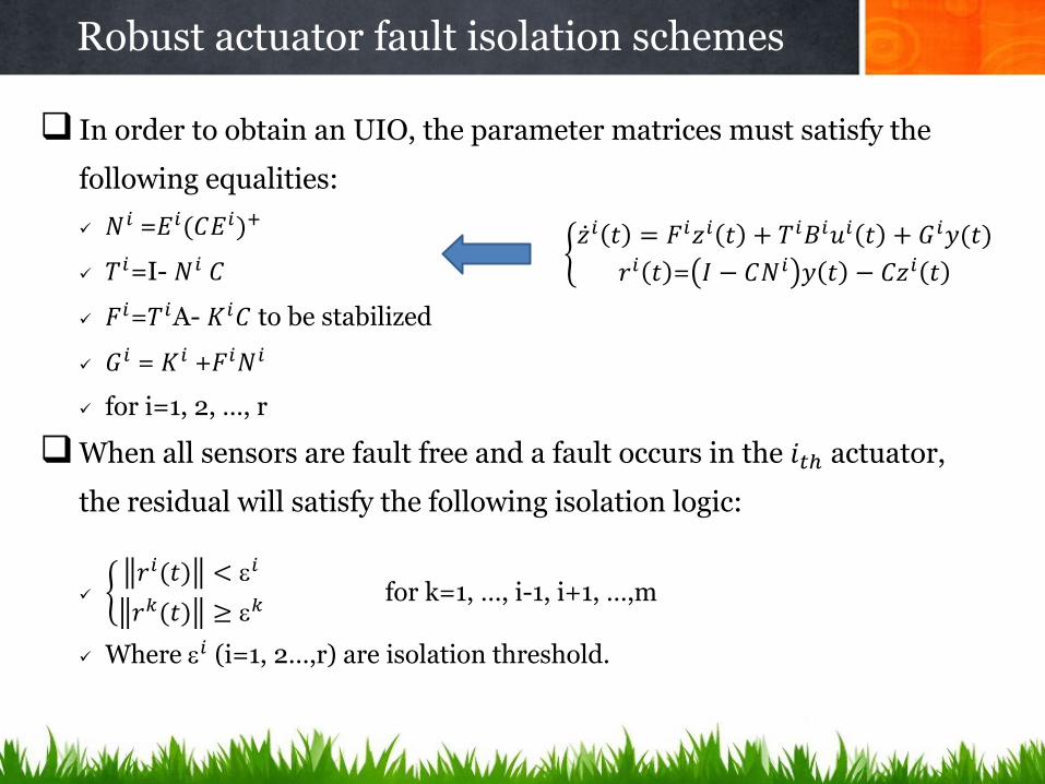
In order to obtain an UIO, the parameter matrices must satisfy the
following equalities:
𝑁𝑖 =𝐸𝑖(𝐶𝐸𝑖)+
𝑇𝑖=I- 𝑁𝑖 𝐶
𝐹𝑖=𝑇𝑖A- 𝐾𝑖𝐶 to be stabilized
𝐺𝑖 = 𝐾𝑖 +𝐹𝑖𝑁𝑖
for i=1, 2, …, r
When all sensors are fault free and a fault occurs in the 𝑖𝑡ℎ actuator,
the residual will satisfy the following isolation logic:
𝑟𝑖(𝑡) < 𝑖
𝑟𝑘(𝑡) ≥ 𝑘 for k=1, …, i-1, i+1, …,m
Where 𝑖 (i=1, 2…,r) are isolation threshold.
Robust actuator fault isolation schemes
𝑧 𝑖 𝑡 = 𝐹𝑖𝑧𝑖 𝑡 + 𝑇𝑖𝐵𝑖𝑢𝑖 𝑡 + 𝐺𝑖𝑦(𝑡)
𝑟𝑖 𝑡 = 𝐼 − 𝐶𝑁𝑖 𝑦 𝑡 − 𝐶𝑧𝑖 𝑡

A robust actuator fault isolation scheme
u
input Actuators Plant Sensors
𝑢𝑅 𝑦𝑅
y
UIO 1
UIO i
⋮
⋮
(𝐼 − 𝐶𝑁1) 𝑦
output
FDI Logic
𝑟1(𝑡)
(𝐼 − 𝐶𝑁𝑖)
(𝐼 − 𝐶𝑁𝑟)
𝑦
𝑦
+
+
+
𝑟𝑖(𝑡)
𝑟𝑟(𝑡)
- 𝐶 𝑧1
- C
𝑧𝑖
- 𝐶 𝑧𝑟
⋮
⋮
Where 𝑟𝑖(𝑡) ∈ 𝑚 i=1, 2 …r
Signal Grouping
𝑢1
𝑢𝑖
𝑢𝑟
UIO r
⋮
⋮
𝑎1
𝑎𝑖
𝑎𝑟
𝑓𝑢

Analysis of the fault actuator isolability
Actuator Generalized Observer Scheme
𝒓𝟏 𝒓𝟐 … 𝒓𝒊 … 𝒓𝒓
𝑓𝑢1 0 1 1 … 1
𝑓𝑢2 1 0 1 … 1
⋮ ⋱ ⋮
𝑓𝑢𝑖 1 1 0 1
⋮ ⋱
𝑓𝑢𝑟 1 1 1 0
Table 1: Generalized Observer Scheme GOS
In the tables above, a "1" in 𝑖𝑡ℎ row and 𝑖𝑡ℎ column denotes that the residual 𝑟𝑖 is sensitive to the fault 𝑓𝑢𝑖, whilst a "0" denotes insensitivity.
𝑎1=1 if 𝑓𝑢1 hold true
Fault alarm 𝑎1 = 𝐿( 𝑟 1 )L( 𝑟2 )L( 𝑟3 ) L( 𝑟𝑚 )
where L( 𝑟𝑖 )=1 if 𝑟𝑖 ≥ 𝑖

Existence condition : In order to satisfy the constraints
𝑇𝑖𝐸𝑖=0 𝑐1 : decoupled condition
𝐹𝑖=𝑇𝑖A- 𝐾𝑖 𝐶 stable 𝑐2 : detectability condition
the following rank conditions must be verified for each UIO:
𝑐1: rank 𝐶𝐸𝑖
𝐸𝑖=rank 𝐶𝐸𝑖 =rank(𝐶[𝐸 𝑏𝑖])=dim(d)+1
𝑐2: rank 𝑝𝐼𝑛 − 𝑇𝑖𝐴𝐶
=n ((𝑇𝑖𝐴))≥0
Robust actuator fault isolation schemes

Remarks
The isolation schemes presented in this previous time can only isolate a
single fault in either a sensor or an actuator, at the same time.
This is based on the fact that the probability for two or more faults to
occurs at the same time is very small in a real situation.
If simultaneous faults need to be isolated, the fault isolation scheme
should be modified based on a regrouping of faults. Each residual will be
designed to be sensitive to one group of faults and insensitive to another
group of faults. See the following Dedicated Observer Scheme (DOS).
A robust sensor fault isolation scheme
Observer-based approaches
Parity (vector) relations
Fault detection via parameter estimation
Residual Generation Techniques

Parity space approach
For static system
Y=CX without UI
For static constraint system
AX=0 Y=CX without UI
For static system without perfect UI decoupled
𝑦𝑘= C𝑥𝑘+𝑘+F𝑑𝑘 𝑦𝑘= C𝑥𝑘+𝑘+𝐹−𝑑−𝑘 +𝐹+𝑑+
𝑘 where 𝑦𝑘
𝑚, 𝑥𝑘𝑛, 𝑘
𝑚, 𝑑𝑘𝑝 are respectively, the measurement vector,
state vector, noise vector and fault vector.
The fault vector is decomposed of two term, 𝑑−𝑘 𝑝−1 denotes the fault vector to
be undetected and 𝑑+𝑘 1 the fault to be detected
Assumption : m > n
Dynamic system
𝑥𝑘+1= A𝑥𝑘+ B𝑢𝑘 + 𝐸1𝑑𝑘 + 𝑅1𝑓𝑘 𝑦𝑘= C𝑥𝑘+ D𝑢𝑘 + 𝐸2𝑑𝑘 + 𝑅2𝑓𝑘 Where 𝑓𝑘
𝑔 denotes a fault vector which may contain actuator, component or sensor faults, 𝑑𝑘
𝑞 denotes the UI (or disturbance) vector.
Parity relation for fault detection and isolation
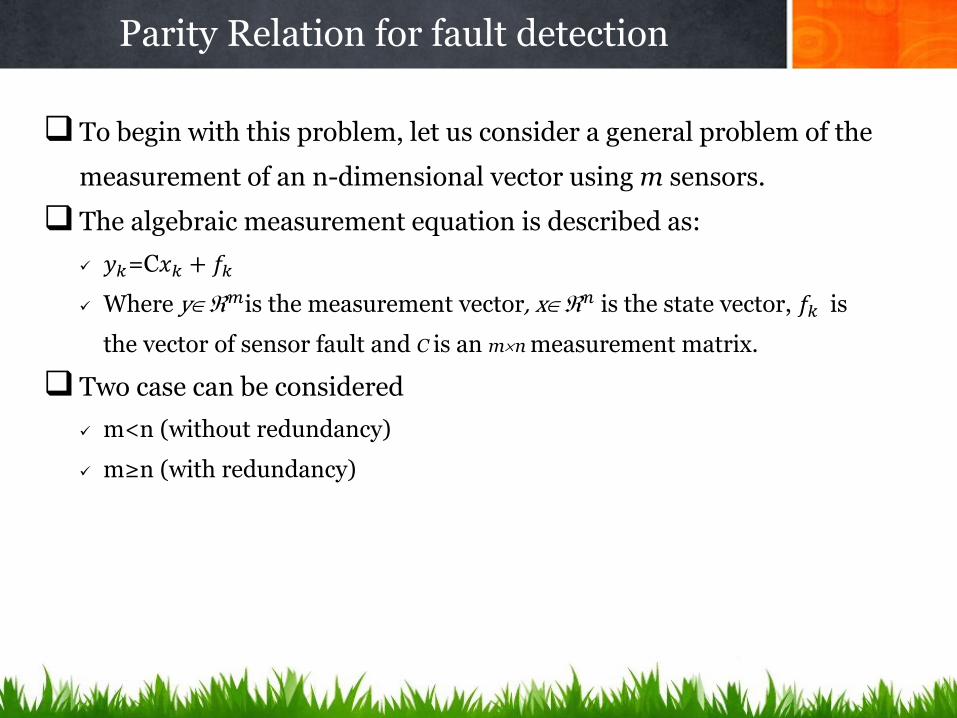
To begin with this problem, let us consider a general problem of the
measurement of an n-dimensional vector using m sensors.
The algebraic measurement equation is described as:
𝑦𝑘=C𝑥𝑘 + 𝑓𝑘
Where y𝑚is the measurement vector, x𝑛 is the state vector, 𝑓𝑘 is
the vector of sensor fault and C is an mn measurement matrix.
Two case can be considered
m<n (without redundancy)
m≥n (with redundancy)
Parity Relation for fault detection

Case 1 : m<n, 𝑦𝑘= 𝐶𝑥𝑘 and rank(C) = m, the direct redundancy
relation does not exist however, we may construct redundancy
relations by collecting sensor outputs over a time interval (data
window):
Y(k-s:k)=
𝑦𝑘−𝑠𝑦𝑘−𝑠+1
⋮𝑦𝑘
This is known as "temporal redundancy" or "serial redundancy". An
example is done at the end of this section.
Parity Relation for fault detection

Case 2 : m≥n and rank(C) = n, this implies that the rows of C are
linearly dependent, i.e., the outputs of the sensors are related by a static
relation.
Example 1:
Isolate a regular of matrix C, as:
Since C1 is invertible, the system becomes
Which is equivalent to
The last relation gives 2 redundancy relation and a third relation can be
obtained
Hence, if a fault occur at sensor 𝑦2, we obtain
and the fault can be detected.
Parity Relation for fault detection
XY
02
11
01
21
02
11
01
2121 C,C
11
122
11
1
22
11
YCCY
XYC
XCY
XCY
02
05.05.00
42
321
2
1112
yy
yyy
Y
YICC
05.05.0 431 yyy
05.05.0
02
05.05.0
431
42
321
yyy
yy
yyy

Example 2 : 𝑦𝑘=C𝑥𝑘 + 𝑓𝑘
The dimension of 𝑦𝑘 is larger than the dimension of 𝑥𝑘, i.e. m> n and
rank(C) = n. For such system configurations, the number of
measurements is greater than the number of variables x.
For FDI purposes, the vector 𝑦𝑘 can be combined into a set of linearly
independent parity equations to generate the parity vector (residual): 𝑟𝑘=V𝑦𝑘=V(C𝑥𝑘 + 𝑓𝑘)
In order to obtain a good characteristic of the residual 𝑟𝑘 (zero-valued for the
fault-free case and insensitive of the unknown x), the matrix V must satisfy
the condition:
VC=0
When this condition holds true, the residual (parity vector) only contains
information on the faults
𝑟𝑘 = 𝑉𝑦𝑘=𝑉𝑓𝑘 𝑟𝑘= 𝑣1𝑓1(𝑘)+ 𝑣2𝑓2(k)+… 𝑣𝑚𝑓𝑚(𝑘)
where 𝑣𝑖 is the column of V, 𝑓𝑖 is the 𝑖𝑡ℎ element of f(k) which denotes
the fault in the 𝑖𝑡ℎ sensor.
Parity Relation for fault detection

Example 3 : 𝑦𝑘= C𝑥𝑘+𝑘+F𝑑𝑘 𝑦𝑘= C𝑥𝑘+𝑘+𝐹−𝑑−𝑘 +𝐹+𝑑+
𝑘
Where the fault vector d is decomposed of two term, 𝑑−𝑘 𝑝−1 denotes
the fault vector to be undetected and 𝑑+𝑘 1 the fault to be detected.
Ideal solution (exact decoupling)
Rewrite the above system as
𝑦𝑘= 𝐶 𝐹−𝑥𝑘
𝑑−𝑘
+ 𝑘 +𝐹+𝑑+𝑘
and find the parity vector P such that
P= 𝑦𝑘= 𝐹+𝑑+𝑘 + 𝑘
𝐶 𝐹− =0
𝐹+0
Therefore P is sensitive to 𝑑+ and insensitive to x and 𝑑−.
Optimization projection (optimal decoupling)
In practice the constraints 𝐶 𝐹− =0 and 𝐹+0 are unfeasible.
One solution is to find an optimal matrix such that :
min
𝐶 𝐹− and max
𝐹+
Parity Relation for fault Isolation
Numerical application

Multi-objective optimization
One of methods to solve the multi-objective optimization problem is to
optimize a new cost function J which accounts for both
𝐽1 = min
𝐶 𝐹− and 𝐽2 = max
𝐹+ . A solution for minimizing J
cannot minimize 𝐽1 at the same time as maximizing 𝐽2.
However, it could lead to a reasonable solution for robust residual design.
A sensible mixture of performance indices is their ratio, i.e.
𝐽 = min
𝐶 𝐹− 2
𝐹+ 2
Hence, the robust residual design is achievable by minimizing J.
Parity Relation for fault Isolation
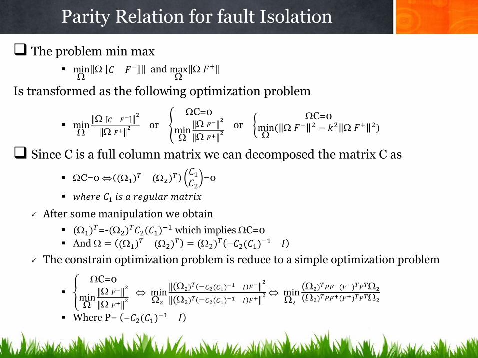
The problem min max
min
𝐶 𝐹− and max
𝐹+
Is transformed as the following optimization problem
min
𝐶 𝐹− 2
𝐹+2 or
C=0
min
𝐹− 2
𝐹+2 or
C=0min
( 𝐹− 2 − 𝑘2 𝐹+ 2)
Since C is a full column matrix we can decomposed the matrix C as
C=0 (1)𝑇 (2)𝑇 𝐶1
𝐶2=0
𝑤ℎ𝑒𝑟𝑒 𝐶1 𝑖𝑠 𝑎 𝑟𝑒𝑔𝑢𝑙𝑎𝑟 𝑚𝑎𝑡𝑟𝑖𝑥
After some manipulation we obtain
(1)𝑇=-(2)𝑇𝐶2(𝐶1)−1 which implies C=0
And = (1)𝑇 (2)𝑇 = (2)𝑇 −𝐶2(𝐶1)−1 𝐼
The constrain optimization problem is reduce to a simple optimization problem
C=0
min
𝐹− 2
𝐹+2 min
2
(2)𝑇 −𝐶2(𝐶1)−1 𝐼 𝐹− 2
(2)𝑇 −𝐶2(𝐶1)−1 𝐼 𝐹+2 min
2
(2)𝑇𝑃𝐹−(𝐹−)𝑇𝑃𝑇2
(2)𝑇𝑃𝐹+(𝐹+)𝑇𝑃𝑇2
Where P= −𝐶2(𝐶1)−1 𝐼
Parity Relation for fault Isolation
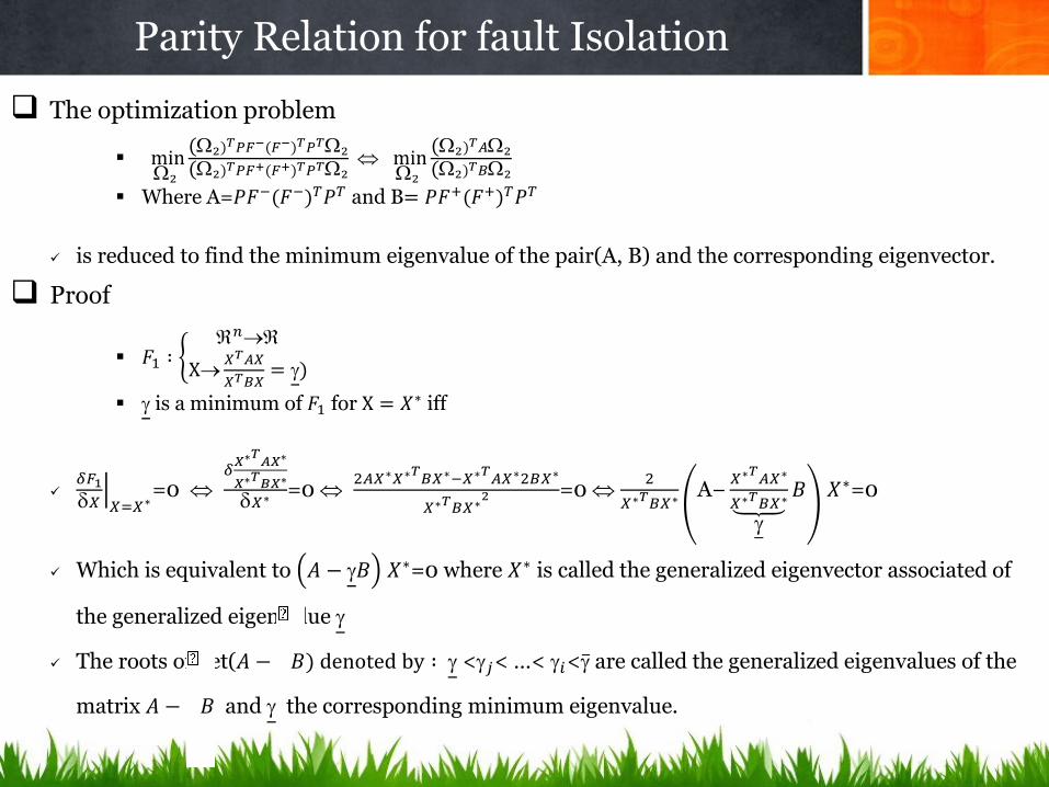
The optimization problem
min2
(2)𝑇𝑃𝐹−(𝐹−)𝑇𝑃𝑇2
(2)𝑇𝑃𝐹+(𝐹+)𝑇𝑃𝑇2 min
2
(2)𝑇𝐴2
(2)𝑇𝐵2
Where A=𝑃𝐹−(𝐹−)𝑇𝑃𝑇 and B= 𝑃𝐹+(𝐹+)𝑇𝑃𝑇
is reduced to find the minimum eigenvalue of the pair(A, B) and the corresponding eigenvector.
Proof
𝐹1 ∶ 𝑛
X𝑋𝑇𝐴𝑋
𝑋𝑇𝐵𝑋= )
is a minimum of 𝐹1 for X = 𝑋∗ iff
𝛿𝐹1
𝑋 𝑋=𝑋∗
=0 𝛿
𝑋∗𝑇𝐴𝑋∗
𝑋∗𝑇𝐵𝑋∗
𝑋∗ =0 2𝐴𝑋∗𝑋∗𝑇
𝐵𝑋∗−𝑋∗𝑇𝐴𝑋∗2𝐵𝑋∗
𝑋∗𝑇𝐵𝑋∗2 =0
2
𝑋∗𝑇𝐵𝑋∗A−
𝑋∗𝑇𝐴𝑋∗
𝑋∗𝑇𝐵𝑋∗
𝐵 𝑋∗=0
Which is equivalent to 𝐴 − 𝐵 𝑋∗=0 where 𝑋∗ is called the generalized eigenvector associated of
the generalized eigenvalue
The roots of det(𝐴 − 𝐵) denoted by ∶ <𝑗< …< 𝑖< are called the generalized eigenvalues of the
matrix 𝐴 − 𝐵 and the corresponding minimum eigenvalue.
Parity Relation for fault Isolation

Consider the discrete-time system with the following description :
Where 𝑢𝑘 ∈ 𝑟 is the known input vector, 𝑦𝑘 ∈ 𝑚 is the known output vector
and 𝑥𝑘 ∈ 𝑛 is the unknown state vector, 𝑓𝑘 ∈ 𝑔 denotes a unknown fault
vector which may contain actuator, component or sensors faults.
𝐴, 𝐵, 𝑅1, 𝑅2, 𝐶 𝑎𝑛𝑑 𝐷 are known real matrices with appropriate dimensions.
How we obtain the redundancy relations ?
Parity Relation for the dynamic systems
𝑥𝑘+1 = 𝐴𝑥𝑘 + 𝐵𝑢𝑘 + 𝑅1𝑓𝑘
𝑦𝑘 = 𝐶𝑥𝑘 + 𝐷𝑢𝑘 + 𝑅2𝑓𝑘
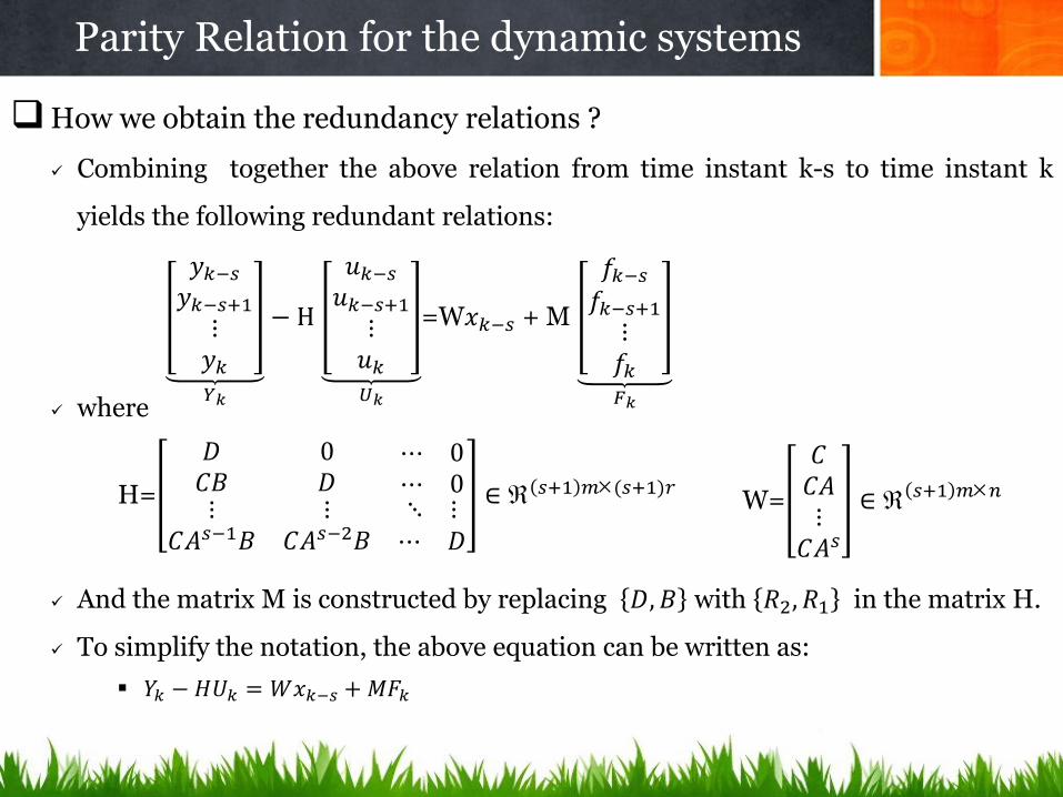
How we obtain the redundancy relations ?
Combining together the above relation from time instant k-s to time instant k
yields the following redundant relations:
where
And the matrix M is constructed by replacing 𝐷, 𝐵 with 𝑅2, 𝑅1 in the matrix H.
To simplify the notation, the above equation can be written as:
𝑌𝑘 − 𝐻𝑈𝑘 = 𝑊𝑥𝑘−𝑠 + 𝑀𝐹𝑘
Parity Relation for the dynamic systems
𝑦𝑘−𝑠
𝑦𝑘−𝑠+1
⋮𝑦𝑘
𝑌𝑘
− H
𝑢𝑘−𝑠
𝑢𝑘−𝑠+1
⋮𝑢𝑘
𝑈𝑘
=W𝑥𝑘−𝑠 + M
𝑓𝑘−𝑠
𝑓𝑘−𝑠+1
⋮𝑓𝑘
𝐹𝑘
H=
𝐷 0 ⋯ 0𝐶𝐵 𝐷 ⋯ 0⋮
𝐶𝐴𝑠−1𝐵⋮
𝐶𝐴𝑠−2𝐵⋱ ⋮
⋯ 𝐷
∈ 𝑠+1 𝑚(𝑠+1)𝑟 W=
𝐶𝐶𝐴⋮
𝐶𝐴𝑠
∈ 𝑠+1 𝑚𝑛

From the following data relation:
𝑌𝑘 − 𝐻𝑈𝑘 = 𝑊𝑥𝑘−𝑠 + 𝑀𝐹𝑘
a residual signal can be defined as:
𝑟𝑘 = 𝑉 𝑌𝑘 − 𝐻𝑈𝑘
Where V ∈ 𝑝 𝑠+1 𝑚 and p is the residual vector dimension. The degree s is called
the order of the parity relation.
In order to analyze the residual, substituting 𝑌𝑘 − 𝐻𝑈𝑘 = 𝑊𝑥𝑘−𝑠 + 𝑀𝐹𝑘 into 𝑟𝑘, we
obtain:
𝑟𝑘 = 𝑉𝑊𝑥𝑘−𝑠 + 𝑉𝑀𝐹𝑘
In order to make the parity vector useful for FDI, one should make it insensitive to
unknown states, i.e.
VW=0
To satisfy the fault detectability condition, the matrix V should also satisfy the
following condition:
VM0
Parity Relation for the dynamic systems

The parity relation approach for residual generation of dynamic system is
shown in the following figure.
Parity Relation for the dynamic systems
System
Memory ‘s’ Samples
H
Memory ‘s’ Samples
V
𝑢𝑘 𝑦𝑘
𝑌𝑘
𝑈𝑘
+
−
𝑟𝑘
Residual generator via temporal redundancy

FDI using the auto-redundance relation approach
Consider the following fault sensor model :
and the decision table
Where
𝑟𝑖𝑘 = 𝑉𝑖 𝑌1𝑘 − 𝐻𝑖𝑈𝑘 = 𝑉𝑖𝑊𝑖𝑥𝑘−𝑠 + 𝑉𝑖𝑀𝑖𝐹𝑖𝑘, i=1, 2, …. m
Parity Relation for the dynamic systems
𝒇𝟏 𝒇𝟐 … 𝒇𝒎
𝑟1 1 0 … 0
𝑟2 0 1 … 0
⋮ ⋮
𝑟𝑚 0 0 … 1
𝑥𝑘+1 = 𝐴𝑥𝑘 + 𝐵𝑢𝑘
𝑦𝑘 = 𝐶𝑥𝑘 + 𝑓𝑘
𝑊𝑖=
𝐶𝑖
𝐶𝑖𝐴⋮
𝐶𝑖𝐴𝑠
H=
0 0 ⋯ 0𝐶𝑖𝐵 0 ⋯ 0⋮
𝐶𝑖𝐴𝑠−1𝐵
⋮𝐶𝑖𝐴
𝑠−2𝐵⋱ ⋮⋯ 0
𝑓𝑖𝑘−𝑠
𝑓𝑖𝑘−𝑠+1
⋮𝑓𝑖𝑘
𝐹𝑖𝑘
Constraints :
𝑉𝑖𝑊𝑖 = 0 𝑉𝑖𝑀𝑖 0

Consider the discrete-time system with the following description :
Where 𝑢𝑘 ∈ 𝑟 is the input vector, 𝑦𝑘 ∈ 𝑚 is the output vector and 𝑥𝑘 ∈ 𝑛 is
the state vector, 𝑓𝑘 ∈ 𝑔 denotes a fault vector which may contain actuator,
component or sensors faults, 𝑑𝑘 ∈ 𝑞 is the unknown input (disturbance) vector.
𝐴, 𝐵, 𝐸1, 𝐸2, 𝑅1, 𝑅2, 𝐶 𝑎𝑛𝑑 𝐷 are known system model matrices with appropriate
dimensions.
In order to detect and isolate the faults a DOS or GOS scheme could be
used.
Parity Relation for the dynamic systems
𝑥𝑘+1 = 𝐴𝑥𝑘 + 𝐵𝑢𝑘 + 𝐸1𝑑𝑘 + 𝑅1𝑓𝑘
𝑦𝑘 = 𝐶𝑥𝑘 + 𝐷𝑢𝑘 + 𝐸2𝑑𝑘 + 𝑅2𝑓𝑘

Observer-based approaches
Parity (vector) relations
Fault detection via parameter estimation
Residual Generation Techniques

The process parameters are not known at all, or they are not known
exactly enough. They can be determined with parameter estimation
methods
The basic structure of the model has to be known
Based on the assumption that the faults are reflected in the physical
system parameters
The parameters of the actual process are estimated on-line using
well-known parameter estimations methods
The results are thus compared with the parameters of the reference
model obtained initially under fault-free assumptions
Any discrepancy (écart) can indicate that a fault may have occurred
Parameter estimation for fault detection

Fault detection of a NL static process via parameter estimation
Example of a Calorimeter
Y=β0 + β1𝑈 + β3𝑈3
The parameters β𝑖 are unknown.
Y = Voltage measure U = Desired Temperature
Objective : Estimated each parameter β
𝑖 by the Least Square (LS) method.
La calorimétrie a pour objet la mesure des quantités de chaleur.
agitateur
Voltage measure Y
U
Measured signals : U(t), Y(t) Basic equation :
Y=β0
+ β1𝑈 + ⋯ + β
𝑞𝑈𝑞
Which is equivalent to Y= 𝑠
𝑇𝑠
𝑠𝑇= β
0β
1… β
𝑞
𝑠𝑇= 1 𝑈 𝑈2 … 𝑈𝑞
Additive faults: 𝑓𝑢input fault; 𝑓𝑦 output fault
Multiplicative faults: β𝑖 parameter faults
First Step : Parameter estimation without fault
An approach for modelling the input-output behavior of the monitored system will be recalled and exploited for fault detection SISO model
Z=H𝜃+ 𝜃 unknown parameter vector noise of the sensor N(0,V) Z sensor H known matrix
Criteria
min𝜃
𝐽( ) = min𝜃
1
2Z−H𝜃 𝑉−1
2 min𝜃
1
2(Z−H𝜃)𝑇𝑉−1(Z−H𝜃)
𝜕𝐽()
𝜕 =
=0 and 𝜕𝐽()
𝜕∗𝜕𝑇>0
Solution
𝜃 =(𝐻𝑇𝑉−1𝐻)−1𝐻𝑇𝑉−1Z
𝜕𝐽()
𝜕∗𝜕𝑇=𝐻𝑇𝑉−1𝐻>0
Example of a Calorimeter
Y=β0 + β1𝑈 + β3𝑈3 Z=H𝜃+
Y= 1 𝑈 𝑈3
β0
β1
β3
+
If V=𝜎2I then 𝜃 =(𝐻𝑇𝐻)−1𝐻𝑇Z=𝐻+𝑍 It’s the Simple LS method
Input/output model
Measured signals:
y(t)=Y(t)-𝑌00; u(t)=U(t)-𝑈00 (Linearized around 𝑌00, 𝑈00)
Basic equation without faults
y(t)+𝑎1𝑦 1 𝑡 + ⋯ + 𝑎𝑛𝑦 𝑛 𝑡 =𝑏0𝑢 𝑡 +𝑏1𝑢 1 𝑡 + ⋯ +𝑏𝑚𝑢 𝑚 𝑡
y(t)=ℎ𝑇 𝑡
ℎ𝑇= −𝑦 1 𝑡 … −𝑦 𝑛 𝑡 𝑢 𝑡 … 𝑢 𝑚 𝑡
𝑇 𝑡 = 𝑎1 … 𝑎𝑛 𝑏0 … 𝑏𝑚
Additive faults
𝑓𝑢 input fault; 𝑓𝑦 output fault
Multiplicative faults
𝑎𝑖 , 𝑏𝑗 𝑝𝑎𝑟𝑎𝑚𝑒𝑡𝑒𝑟𝑠 𝑓𝑎𝑢𝑙𝑡𝑠
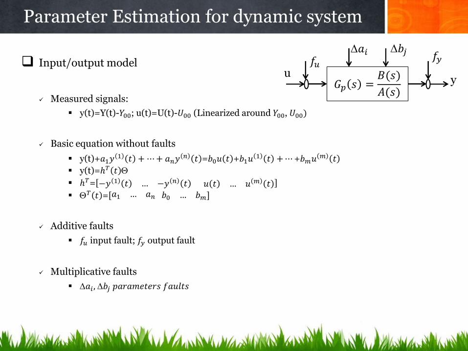
Parameter Estimation for dynamic system
𝐺𝑝 𝑠 =𝐵(𝑠)
𝐴(𝑠)
𝑓𝑦 𝑓𝑢 u
y
𝑎𝑖 𝑏𝑗

Spate space model
Basic equation
𝑥(𝑡) =Ax(t)+bu(t)
y(t)= 𝑐𝑇x(t)
A=
0 0 10 1 −𝑎1
1⋮
0⋮
−𝑎2
⋮
𝑏𝑇= 𝑏0 𝑏1 …
𝑐𝑇= 0 0 … 1
Additive fault
𝑓𝑙 input or state variable fault
𝑓𝑚 output fault
Multiplicative fault
A, B, c parameter faults
Parameter Estimation for dynamic system
b
𝑏𝑖
u
𝑥 𝑐𝑇
𝑐𝑗 m
𝑓𝑚
y x
A
𝑎𝑖
I
𝑓𝑙
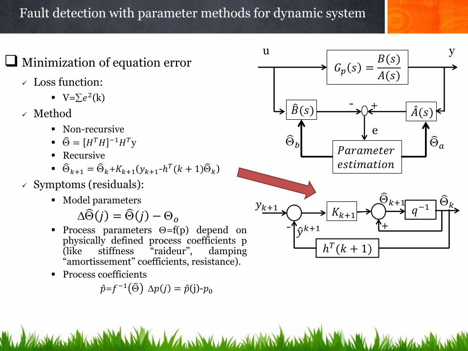
Minimization of equation error
Loss function:
V=𝑒2(k)
Method
Non-recursive
= 𝐻𝑇𝐻 −1𝐻𝑇y
Recursive
𝑘+1 = 𝑘+𝐾𝑘+1(𝑦𝑘+1-ℎ𝑇(𝑘 + 1) 𝑘)
Symptoms (residuals):
Model parameters
𝑗 = 𝑗 − 𝑜 Process parameters =f(p) depend on
physically defined process coefficients p (like stiffness “raideur”, damping “amortissement” coefficients, resistance).
Process coefficients
𝑝 =𝑓−1 𝑝 𝑗 = 𝑝 (j)-𝑝0
Fault detection with parameter methods for dynamic system
𝐺𝑝 𝑠 =𝐵(𝑠)
𝐴(𝑠)
u y
𝐵 (𝑠) 𝐴 (𝑠)
𝑃𝑎𝑟𝑎𝑚𝑒𝑡𝑒𝑟 𝑒𝑠𝑡𝑖𝑚𝑎𝑡𝑖𝑜𝑛
𝑏 𝑎 e
+ -
𝐾𝑘+1 𝑦𝑘+1
𝑦 𝑘+1
ℎ𝑇(𝑘 + 1)
𝑞−1 𝑘 𝑘+1
+ -

Proof of Non-recursive LS method
Consider an ARX model
𝐴 𝑞 𝑦 𝑡 = 𝐵 𝑞 𝑢 𝑡 + (𝑡)
where
𝐴 𝑞 = 1 + 𝑎1𝑞−1+⋯ + 𝑎𝑛𝑎𝑞−𝑛𝑎
B 𝑞 = 𝑏1𝑞−1+⋯ + 𝑏𝑛𝑏𝑞−𝑛𝑏
= 𝑁(0, 2)
Basic equation
𝑦 𝑡 = ℎ𝑇(t)+ (t)
where ℎ𝑇(t)=[-y(t-1) … -y(t-𝑛𝑎) u(t-1) … u(t-𝑛𝑏)] and 𝑇 = [𝑎1 … 𝑎𝑛𝑎 𝑏1 … 𝑏𝑛𝑏]
Data record
Fault detection with parameter methods for dynamic system
)(
)(
)1(
1
1
)()1(1
)()1(21
)1()0(110
)(
)(
1
t
k
nb
na
nbttnatt
nbkknakkk
nbna
b
b
a
a
uuyy
uuyyy
uuyyy
ty
ky
y
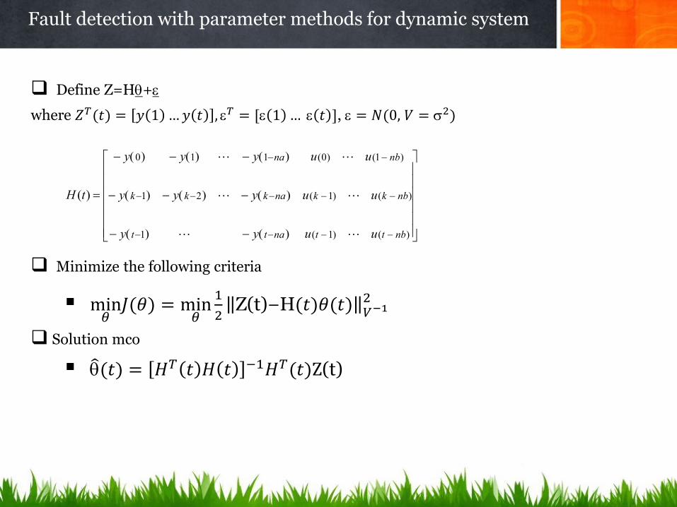
Define Z=H+
where 𝑍𝑇(𝑡) = 𝑦 1 … 𝑦 𝑡 , 𝑇 = [ 1 … 𝑡 ], = 𝑁(0, 𝑉 = 2)
Minimize the following criteria
min𝜃
𝐽(𝜃) = min𝜃
1
2Z(t)−H(𝑡)𝜃(𝑡) 𝑉−1
2
Solution mco
(𝑡) = 𝐻𝑇 𝑡 𝐻 𝑡 −1𝐻𝑇(𝑡)Z(t)
Fault detection with parameter methods for dynamic system
)()1(1
)()1(21
)1()0(110
)(
nbttnatt
nbkknakkk
nbna
uuyy
uuyyy
uuyyy
tH

Proof of Recursive LS method
Data record
Which is equivalent to
From the previous results, we obtain
(𝑡 + 1) = 𝐻𝑇 𝑡 + 1 𝐻 𝑡 + 1 −1𝐻𝑇(𝑡 + 1)Z(t+1)
Fault detection with parameter methods for dynamic system
)1(
)(
)(
)1(
1
1
)()(1
)()1(1
)()1(21
)1()0(110
)1(
)(
)(
1
t
t
k
nb
na
nbttnatt
nbttnatt
nbkknakkk
nbna
b
b
a
a
uuyy
uuyy
uuyyy
uuyyy
ty
ty
ky
y
)1(
)(
)1(
)(
)1(
)(
t
t
T th
tH
ty
tZ
)1()1()()()1()1()()(1ˆ
)1(
)()1()(
)1(
)()1()(1ˆ
1
1
tythtZtHththtHtHt
ty
tZthtH
th
tHthtHt
TTT
TT
T

Proof of Recursive LS method
Using the matrix inversion Lemma, the relation
Becomes
where
Fault detection with parameter methods for dynamic system
)1()1()()()1()1()()(1ˆ1
tythtZtHththtHtHt TTT
)(ˆ)1()1(
)1()()()1(1
)1()()(ˆ1ˆ1
1
tthty
thtHtHth
thtHtHtt T
TT
T
𝐾𝑡+1 𝑦𝑡+1
𝑦 𝑡+1
ℎ𝑇(𝑡 + 1)
𝑞−1 𝑡 𝑡+1
+ -
)1()()1(1
)()1()1()()()1()1()()()1()1()1(
)()()(
)1()()1(1
)1()(
11
1
1
thtPth
tPththtPtPththtHtHtHtHtP
tHtHtP
thtPth
thtPK
T
TTTT
T
Tt
)1(ˆ)1(ˆ1ˆ1 tytyKtt t
Prediction error Gain factor
1111111 DABDACBAABCDA
Matrix inversion Lemma
)1(,1),1(),()( thDCthBtHtHA TT
Fault detection with parameter methods for dynamic system
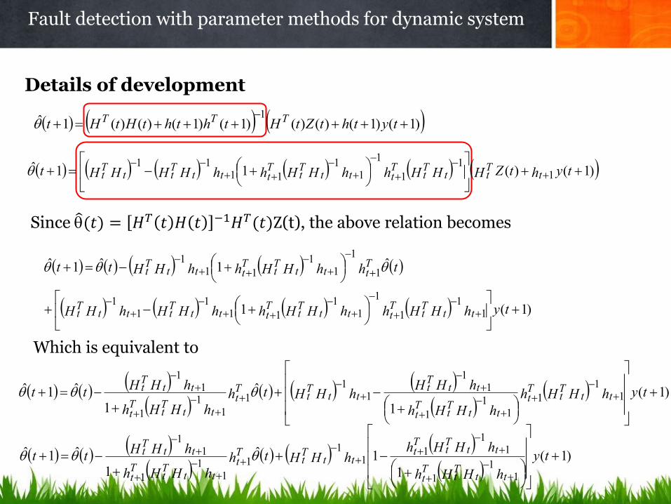
Details of development
)1()(11ˆ1
1
1
1
11
1111
tyhtZHHHhhHHhhHHHHt tTtt
Tt
Tttt
Tt
Tttt
Ttt
Tt
)1()1()()()1()1()()(1ˆ1
tythtZtHththtHtHt TTT
Since (𝑡) = 𝐻𝑇 𝑡 𝐻 𝑡 −1𝐻𝑇(𝑡)Z(t), the above relation becomes
)1(
1
ˆ
1
ˆ1ˆ1
1
1
11
1
11
11
1
11
1
11
tyhHHh
hHHh
hHHhHHth
hHHh
hHHtt tt
Tt
Tt
ttTt
Tt
ttTt
ttTt
Tt
ttTt
Tt
ttTt
)1(1
ˆ1ˆ1ˆ
11
1
1
11
111
11
1
1
11
111
tyhHHhhHHhhHHhHH
thhHHhhHHtt
ttTt
Tttt
Tt
Tttt
Tttt
Tt
Tttt
Tt
Tttt
Tt
Which is equivalent to
)1(
1
1ˆ
1
ˆ1ˆ
11
1
11
11
1
1
11
1
11
ty
hHHh
hHHhhHHth
hHHh
hHHtt
ttTt
Tt
ttTt
Tt
ttTt
Tt
ttTt
Tt
ttTt
Fault detection with parameter methods for dynamic system
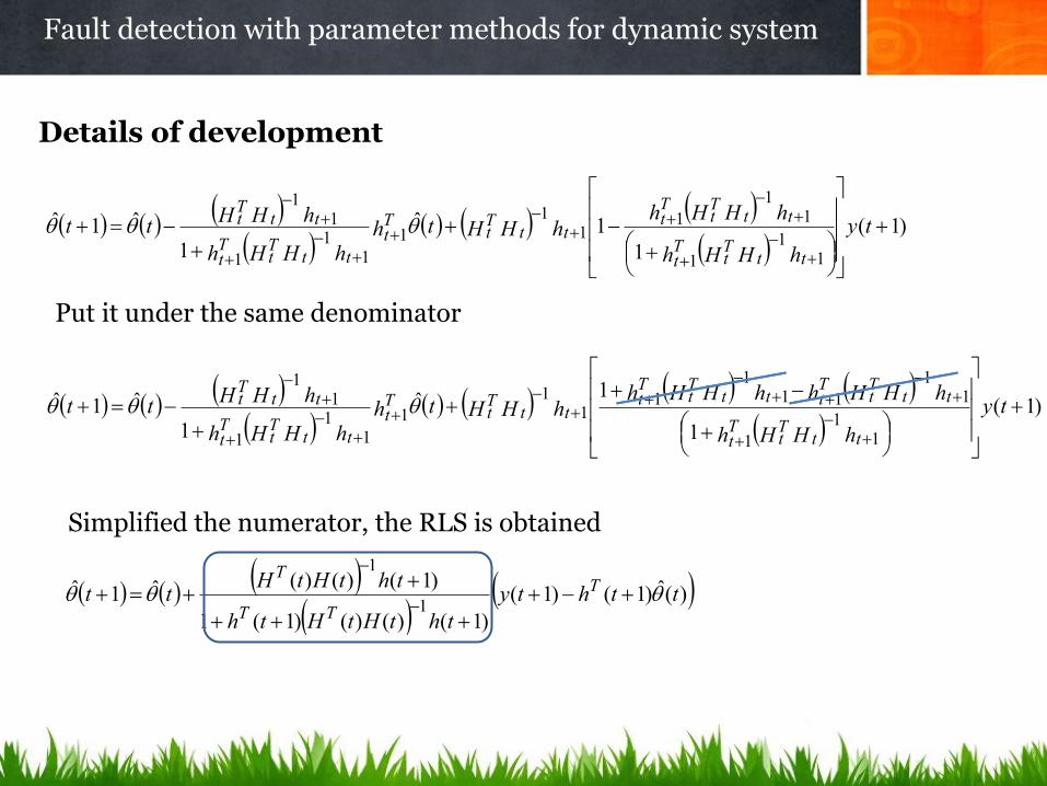
Details of development
)1(
1
1ˆ
1
ˆ1ˆ
11
1
11
11
1
1
11
1
11
ty
hHHh
hHHhhHHth
hHHh
hHHtt
ttTt
Tt
ttTt
Tt
ttTt
Tt
ttTt
Tt
ttTt
)1(
1
1ˆ
1
ˆ1ˆ
11
1
11
111
11
1
1
11
1
11
ty
hHHh
hHHhhHHhhHHth
hHHh
hHHtt
ttTt
Tt
ttTt
Tttt
Tt
Tt
ttTt
Tt
ttTt
Tt
ttTt
)(ˆ)1()1(
)1()()()1(1
)1()()(ˆ1ˆ1
1
tthty
thtHtHth
thtHtHtt T
TT
T
Put it under the same denominator
Simplified the numerator, the RLS is obtained

Consider the following circuit system
Assign 𝑏0 = 1, 𝑏1 = 𝐶 𝑎𝑛𝑑 𝑎1 = 𝑅𝐶
In case 1, we consider 𝑢1 and 𝑢2 as the output measurements :
𝑏0 𝑢1(t)= 𝑢2 𝑡 + 𝑎1𝑑𝑢2(𝑡)
𝑑𝑡
Using the LS method we obtain an estimate of 𝑇=[𝑏0 𝑎1].
The process coefficient 𝑝 =𝑓−1 is not available
In case 2, we consider 𝑢1 and 𝑖 as the output measurements :
𝑏1 𝑑𝑢1(𝑡)
𝑑𝑡= 𝑎1
𝑑𝑖(𝑡)
𝑑𝑡+i(t)
Using the LS method we obtain an estimate of 𝑇=[𝑏1 𝑎1].
The process coefficient 𝑝 =𝑓−1 is available : 𝑝 𝑇=[R C]
Exercise :
Describes the LS procedure
Gives the parameter residual
Application of the LS method
R
C 𝑢2 𝑢1
i

Case 2 :
𝐶 𝑑𝑢1(𝑡)
𝑑𝑡= 𝑅𝐶
𝑑𝑖(𝑡)
𝑑𝑡+i(t)
Using an implicit Euler approximation
𝐶 𝑢1𝑛+1−𝑢1𝑛
𝑡-RC
𝑖𝑛+1−𝑖𝑛
𝑡= 𝑖𝑛+1
𝑖𝑛+1= −𝑖𝑛+1−𝑖𝑛
𝑡
𝑢1𝑛+1−𝑢1𝑛
𝑡
𝑅𝐶𝐶
Application of the LS method
R
C 𝑢2 𝑢1
i
M T K T F
1
...
n nT T T
T tt t
Numeric modelisation : (Mathematical Lecturer of UTC)

Robust residual generation for model-based fault diagnosis of dynamic
systems, phd Thesis of Jie Chen, 1995.
Robust Model based fault diagnosis for dynamic systems, by Jie Chen and
R.J. Patton, Edition Springer 1999.
Fault diagnosis of dynamic systems using model-based and filtering
approaches by Silvio Simani 2006.
Model-based Fault Diagnosis Techniques Design Schemes, Algorithms,
and Tools, by Steven X. Ding, Edition Springer 2007
Fault – Diagnosis Applications, by Rolf Isermann, Edition Springer 2011.
Bibliography