AC STEADY-STATE ANALYSISLEARNING GOALS

SINUSOIDSReview basic facts about sinusoidal signals

SINUSOIDAL AND COMPLEX FORCING FUNCTIONSBehavior of circuits with sinusoidal independent sourcesand modeling of sinusoids in terms of complex exponentials

PHASORSRepresentation of complex exponentials as vectors. It facilitatessteady-state analysis of circuits.

IMPEDANCE AND ADMITANCEGeneralization of the familiar concepts of resistance and conductance to describe AC steady state circuit operation

PHASOR DIAGRAMSRepresentation of AC voltages and currents as complex vectors

BASIC AC ANALYSIS USING KIRCHHOFF LAWS

ANALYSIS TECHNIQUESExtension of node, loop, Thevenin and other techniques

SINUSOIDS

tXtx M ωsin)( =

(radians)argument (rads/sec)frequency angular

valuemaximumor amplitude

===

t

X M

ωω

Adimensional plot As function of time

tTtxtxT ∀+=⇒== ),()(2 Period ωπ

)(cycle/sec Hertz infrequency ===πω2

1T

f

fπω 2=

"by leads" θ

"by lags" θ

BASIC TRIGONOMETRY

)cos(21)cos(

21coscos

)sin(21)sin(

21cossin

sinsincoscos)cos(sincoscossin)sin(

βαβαβα

βαβαβα

βαβαβαβαβαβα

−++=

−++=

+=−−=−

IDENTITIES DERIVED SOME

αααα

βαβαβαβαβαβα

cos)cos(sin)sin(

sinsincoscos)cos(sincoscossin)sin(

=−−=−

−=++=+

IDENTITIESESSENTIAL

)sin(sin)cos(cos

)2

cos(sin

)2

sin(cos

πωωπωω

πωω

πωω

±−=±−=

−=

+=

tttt

tt

tt

NSAPPLICATIO

)90sin()2

sin( °+=+ tt ωπω

CONVENTION EE ACCEPTED

RADIANS AND DEGREES

(degrees) 180(rads)

degrees360 radians

θπ

θ

π

=

=2

LEARNING EXAMPLE

)45cos( °+tω

)cos( tω

Leads by 45 degrees

)45cos( °+− tω)18045cos( ±+tω

Leads by 225 or lags by 135

)36045cos( −+tω

Lags by 315

LEARNING EXAMPLE

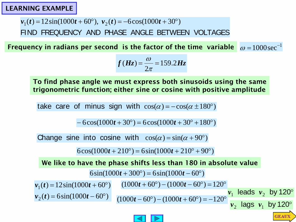
VOLTAGESBETWEEN ANGLEPHASE ANDFREQUENCY FIND)301000cos(6)(),601000sin(12)( 21 °+−=°+= ttvttv

Frequency in radians per second is the factor of the time variable 1sec1000 −=ω

HzHzf 2.1592

)( ==πω

To find phase angle we must express both sinusoids using the sametrigonometric function; either sine or cosine with positive amplitude

)180301000cos(6)301000cos(6 °+°+=°+− tt

)180cos()cos( °±−= αα with sign minus of care take

)90sin()cos( °+= αα with cosine into sine Change

)902101000sin(6)2101000cos(6 °+°+=°+ ttWe like to have the phase shifts less than 180 in absolute value

)601000sin(6)3001000sin(6 °−=°+ tt

)601000sin(6)()601000sin(12)(

2

1

°−=°+=

ttvttv °=°−−°+ 120)601000()601000( tt

°120by leads 21 vv°−=°+−°− 120)601000()601000( tt

°120by lags 12 vv

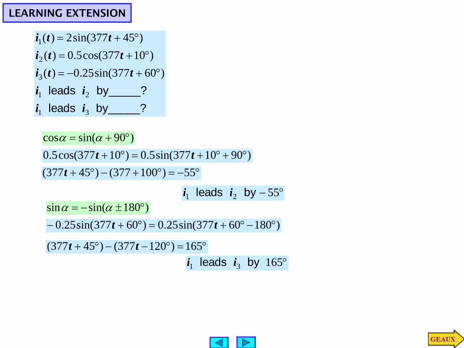
LEARNING EXTENSION

by_____? leads by_____? leads

31

21

3

2

1

)60377sin(25.0)()10377cos(5.0)(

)45377sin(2)(

iiii

ttitti

tti

°+−=°+=

°+=

)90sin(cos °+= αα)9010377sin(5.0)10377cos(5.0 °+°+=°+ tt

°−=°+−°+ 55)100377()45377( t

°− 5521 by leads ii

°16531 by leads ii

)180sin(sin °±−= αα)18060377sin(25.0)60377sin(25.0 °−°+=°+− tt

°=°−−°+ 165)120377()45377( tt

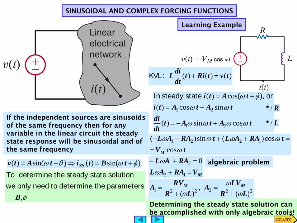
SINUSOIDAL AND COMPLEX FORCING FUNCTIONS

If the independent sources are sinusoidsof the same frequency then for anyvariable in the linear circuit the steadystate response will be sinusoidal and ofthe same frequency

)sin()()sin()( φωθω +=⇒+= tBtitAtv SS

φ,B parameters the determine to needonly wesolutionstatesteady the determine To

Learning Example

)()()( tvtRitdtdiL =+ :KVL

tAtAtdtdi

tAtAtitAti

ωωωω

ωωφω

cossin)(

sincos)()cos()(

21

21

+−=

+=+= or,statesteady In

R/*

L/*

tVtRAALtRAAL

M ωωωωω

coscos)(sin)( 1221

==+++−

MVRAALRAAL

=+=+−

12

21 0ωω algebraic problem

222221 )(,

)( LRLVA

LRRVA MM

ωω

ω +=

+=

Determining the steady state solution canbe accomplished with only algebraic tools!

FURTHER ANALYSIS OF THE SOLUTION

)cos()(cos)(

sincos)( 21

φωωωω

+==

+=

tAtitVtv

tAtAti

M

write can one purposes comparisonFor is voltageapplied The

issolution The

φφ sin,cos 21 AAAA −==

222221 )(,

)( LRLVA

LRRVA MM

ωω

ω +=

+=

1

222

21 tan,

AAAAA −=+= φ

RL

LRVA M ωφω

122 tan,

)(−=

+=

)tancos()(

)( 122 R

LtLR

Vti M ωωω

−−+

=

voltagethelags WAYScurrent ALtheFor 0≠L

90by voltagethelagscurrent theinductor)(pure If °= 0R

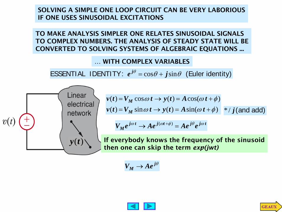
SOLVING A SIMPLE ONE LOOP CIRCUIT CAN BE VERY LABORIOUSIF ONE USES SINUSOIDAL EXCITATIONS

TO MAKE ANALYSIS SIMPLER ONE RELATES SINUSOIDAL SIGNALSTO COMPLEX NUMBERS. THE ANALYSIS OF STEADY STATE WILL BECONVERTED TO SOLVING SYSTEMS OF ALGEBRAIC EQUATIONS ...

… WITH COMPLEX VARIABLES

)(ty

)sin()(sin)()cos()(cos)(

φωωφωω

+=→=+=→=

tAtytVtvtAtytVtv

M

M

identity)(Euler :IDENTITY ESSENTIAL θθθ sincos je j +=

tjjtjtjM eAeAeeV ωθφωω =→ + )(

add)(andj/*

θjM AeV →

If everybody knows the frequency of the sinusoidthen one can skip the term exp(jwt)

Learning Example

tjM eVtv ω=)(

)()( φω += tjM eIti Assume

)()()( tvtRitdtdiL =+ :KVL

)()( φωω += tjM eIjt

dtdi

tjjM

tjM

tjM

tjM

eeIRLj

eIRLj

eRIeLIjtRitdtdiL

ωφ

φω

φωφω

ω

ω

ω

)(

)(

)()(

)(

)()(

+=

+=

+=+

+

++

tjM

tjjM eVeeIRLj ωωφω =+ )(

RLjVeI Mj

M +=

ωφ

LjRLjR

ωω

−−/*

22 )()(

LRLjRVeI Mj

M ωωφ

+−

=

RL

eLRLjRω

ωω1tan22 )(−−

+=−

RL

MjM e

LRVeI

ωφ

ω

1tan

22 )(

−−

+=

RL

LRVI M

Mωφ

ω1

22tan,

)(−−=

+=

)cos(}Re{)(

}Re{cos)()( φω

ωφω

ω

−==⇒

==− tIeIti

eVtVtv

Mtj

M

tjMM

θθ

θ

θ

sin,cos

tan, 122

ryrxyxyxr

rejyx

PCj

==

=+=

=+

↔

−

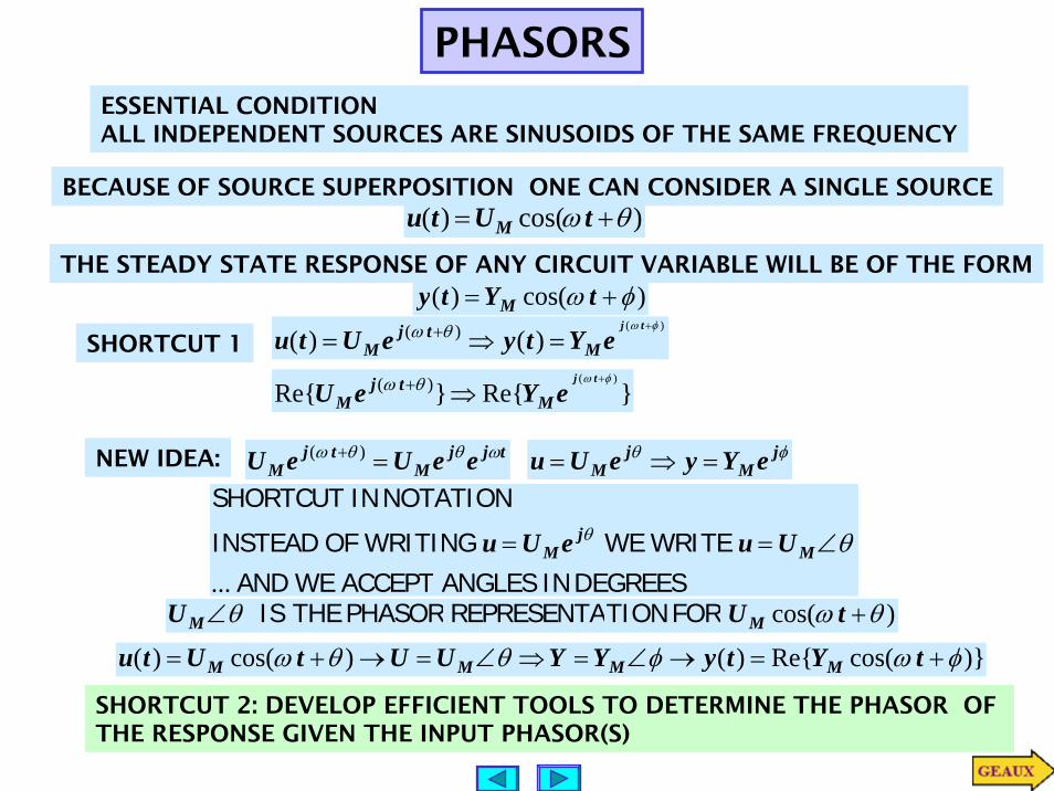
PHASORSESSENTIAL CONDITIONALL INDEPENDENT SOURCES ARE SINUSOIDS OF THE SAME FREQUENCY

BECAUSE OF SOURCE SUPERPOSITION ONE CAN CONSIDER A SINGLE SOURCE)cos()( θω += tUtu M

THE STEADY STATE RESPONSE OF ANY CIRCUIT VARIABLE WILL BE OF THE FORM)cos()( φω += tYty M

SHORTCUT 1)(

)()( )( φωθω +

=⇒= + tj

eYtyeUtu Mtj

M

}Re{}Re{)()( φωθω +

⇒+ tj

eYeU Mtj

M

NEW IDEA: tjjM

tjM eeUeU ωθθω =+ )( φθ j

Mj

M eYyeUu =⇒=

DEGREESINANGLESACCEPTWE AND WRITE WE WRITING OF INSTEAD

NOTATIONINSHORTCUT

...θθ ∠== M

jM UueUu

)cos( θωθ +∠ tUU MM FORTIONREPRESENTAPHASORTHEIS

)}cos(Re{)()cos()( φωφθθω +=→∠=⇒∠=→+= tYtyYYUUtUtu MMMM

SHORTCUT 2: DEVELOP EFFICIENT TOOLS TO DETERMINE THE PHASOR OF THE RESPONSE GIVEN THE INPUT PHASOR(S)

Learning Example

tjM

Vev

VVω=

∠= 0

tjM

Iei

IIω

φ

=

∠=

tjtjtj VeRIeIejL

vtRitdtdiL

ωωωω =+

=+

)(

)()(

LjRVI

VRILIj

ω

ω

+=

=+hasonephasors of termsIn

The phasor can be obtained usingonly complex algebra

We will develop a phasor representationfor the circuit that will eliminate the needof writing the differential equation

°−±∠↔±±∠↔±

90)sin()cos(

θθωθθω

AtAAtA

It is essential to be able to move fromsinusoids to phasor representation

Learning Extensions

↔°−= )425377cos(12)( ttv °−∠ 42512↔°+= )2.42513sin(18)( tty °−∠ 8.8518

↔°∠==2010

400

1VHzf Given

)20800cos(10)(1 °+= ttv π↔°−∠= 60122V )60800cos(12)(2 °−= ttv π

Phasors can be combined using therules of complex algebra

)())(( 21212211 θθθθ +∠=∠∠ VVVV

)( 212

1

22

11 θθθθ

−∠=∠∠

VV

VV

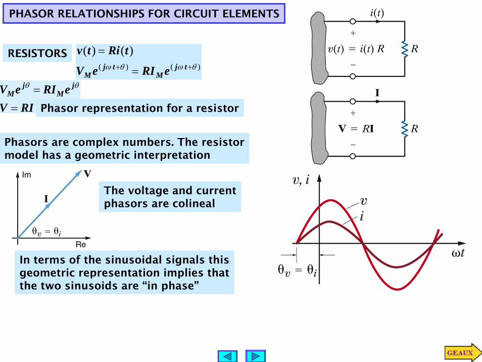
PHASOR RELATIONSHIPS FOR CIRCUIT ELEMENTS

RESISTORS)()(

)()(θωθω ++ =

=tj

Mtj

M eRIeV

tRitv

RIVeRIeV j

Mj

M

== θθ

Phasor representation for a resistor

Phasors are complex numbers. The resistormodel has a geometric interpretation

The voltage and currentphasors are colineal

In terms of the sinusoidal signals thisgeometric representation implies thatthe two sinusoids are “in phase”

INDUCTORS )( )()( φωθω ++ = tjM

tjM eI

dtdLeV

)( φωω += tjM eLIj

LIjV ω=

The relationship betweenphasors is algebraic

°=°∠= 90901 jej

For the geometric viewuse the result

°∠= 90LIV ω

The voltage leads the current by 90 degThe current lags the voltage by 90 deg

φθ ω jM

jM eLIjeV =

Learning Example

)().20377cos(12)(,20 tittvmHL Find °+==

LjVI

V

ω

ω

=

°∠==

2012377

)(902012 A

LI

°∠°∠

=ω

)(701020377

123 AI °−∠

××= −

)70377cos(1020377

12)( 3 °−××

= − tti

Relationship between sinusoids

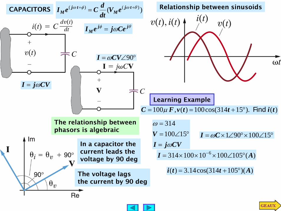
CAPACITORS )( )()( θωφω ++ = tjM

tjM eV

dtdCeI

θφ ω jjM CejeI =

CVjI ω=

The relationship betweenphasors is algebraic

°∠= 90CVI ω

In a capacitor thecurrent leads thevoltage by 90 deg

The voltage lagsthe current by 90 deg

CVjIV

ω

ω

=°∠=

=15100

314

°∠×°∠×= 15100901CI ω

)(10510010100314 6 AI °∠×××= −

))(105314cos(14.3)( Atti °+=

Relationship between sinusoids

Learning Example

)().15314cos(100)(,100 tittvFC Find °+== μ

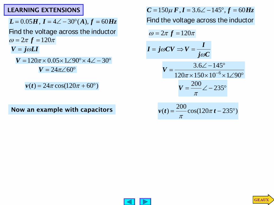
LEARNING EXTENSIONS

inductor the across voltagethe FindHzfAIHL 60),(304,05.0 =°−∠==

ππω 1202 == fLIjV ω=

°−∠×°∠××= 30490105.0120πV°∠= 6024πV

)60120cos(24)( °+= ππtv

inductor the across voltagethe FindHzfIFC 60,1456.3,150 =°−∠== μ

ππω 1202 == f

CjIVCVjIω

ω =⇒=

°∠×××°−∠

= − 901101501201456.3

6πV

°−∠= 235200π

V

)235120cos(200)( °−= ttv ππ

Now an example with capacitors

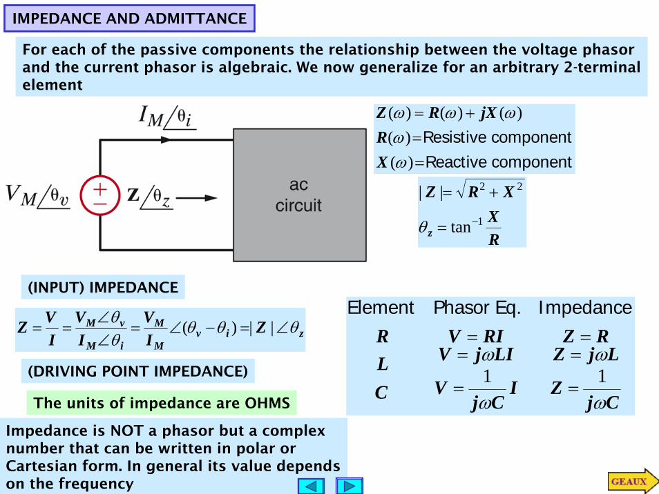
IMPEDANCE AND ADMITTANCE

For each of the passive components the relationship between the voltage phasorand the current phasor is algebraic. We now generalize for an arbitrary 2-terminalelement

zivM

M

iM

vM ZIV

IV

IVZ θθθ

θθ

∠=−∠=∠∠

== ||)(

(INPUT) IMPEDANCE

(DRIVING POINT IMPEDANCE)

The units of impedance are OHMS CjZ

LjZ

ICj

V

LIjV

CL

RZRIVR

ω

ω

ω

ω11

=

=

=

===

ImpedanceEq.Phasor Element

Impedance is NOT a phasor but a complexnumber that can be written in polar or Cartesian form. In general its value dependson the frequency

component Reactivecomponent Resistive

==

+=

)()(

)()()(

ωω

ωωω

XR

jXRZ

RX

XRZ

z1

22

tan

||

−=

+=

θ

KVL AND KCL HOLD FOR PHASOR REPRESENTATIONS

−

+)(1 tv

−

+)(3 tv

−+ )(2 tv)(0 ti

)(1 ti )(2 ti )(3 ti

0)()()( 321 =++ tvtvtv :KVL

3,2,1,0,)(

0)()()()()(

3210

==

=+++−+ keIti

titititiktj

Mkkφω

:KCL

3,2,1,)( )( == + ieVtv itjMii

θω

0)( 321321 =++ tjj

Mj

Mj

M eeVeVeV ωθθθ :KVL

0332211 =∠+∠+∠ θθθ MMM VVV

Phasors! 0321 =++ VVV

−

+

1V−

+

3V

−+ 2V0I

1I 2I 3I

03210 =+++− IIII

The components will be represented by their impedances and the relationshipswill be entirely algebraic!!

In a similar way, one shows ...

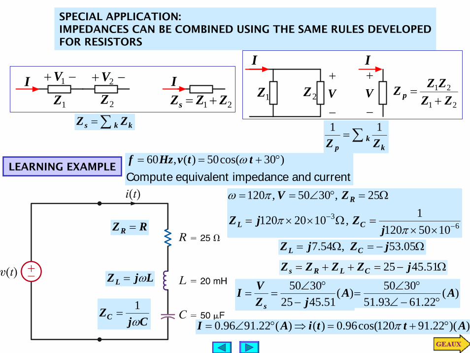
SPECIAL APPLICATION:IMPEDANCES CAN BE COMBINED USING THE SAME RULES DEVELOPEDFOR RESISTORS

I −+ 1V

1Z

−+ 2V

2ZI

21 ZZZs += 1Z 2Z−

+V

I I

−

+V

21

21

ZZZZZ p +

=

∑= kks ZZ∑=

kk

p ZZ11

LEARNING EXAMPLEcurrent and impedance equivalent Compute

)30cos(50)(,60 °+== ttvHzf ω

63

10501201,1020120

25,3050,120

−−

××=Ω××=

Ω=°∠==

ππ

πω

jZjZ

ZV

CL

R

Ω−=Ω= 05.53,54.7 jZjZ CL

Ω−=++= 51.4525 jZZZZ CLRs

)(51.4525

3050 AjZ

VIs −

°∠== )(

22.6193.513050 A

°−∠°∠

=

))(22.91120cos(96.0)()(22.9196.0 AttiAI °+=⇒°∠= π

RZR =

LjZL ω=

CjZC ω

1=

LEARNING EXTENSION )(ti FIND

377=ω

°−∠= )9060(120V

Ω= 20RZ

Ω=××= − 08.151040377 3 jjZL

05.531050377 6 jjZC −=

××= −

)(|| LRCeq ZZZZ += °∠== 239.9963.3097144561630 . + j.Zeq

)(924.39876.3239.9963.30

30120 AZVI

eq°−∠=

°∠°−∠

==

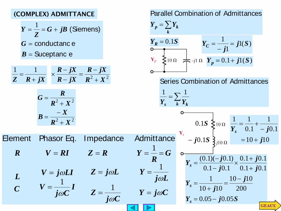
(COMPLEX) ADMITTANCE

eSuceptanc econductanc

(Siemens)

==

+==

BG

jBGZ

Y 1

jXRZ +=

1122 XR

jXRjXRjXR

+−

=−−

×

22

22

XRXB

XRRG

+−

=

+=

CjYCj

Z

LjYLjZ

ICj

V

LIjV

CL

GR

YRZRIVR

ωω

ωω

ω

ω

==

==

=

=

====

1

1

1

1AdmittanceImpedanceEq.Phasor Element

∑=k

kp YYesAdmittancofnCombinatioParallel

∑=k ks YY

11esAdmittancofnCombinatioSeries

SYR 1.0= )(11

1 Sjj

YC =−

=

)(11.0 SjYp +=

10101.0

11.0

11

jjYs

+=−

+=

SjY

jj

Y

jj

jjY

s

s

s

05.005.0200

10101010

11.01.01.01.0

1.01.0)1.0)(1.0(

−=

−=

+=

++

×−−

=

S1.0

Sj 1.0−

LEARNING EXAMPLE

IYVV

p

S

,)(4560

FIND°∠=

4242

jjZ p +

×= )(25.05.0

842 Sj

jjYp −=

+=

)(4560)25.05.0( AjVYI p °∠×−==

)(4560565.26559.0 AI °∠×°−∠=

)(435.1854.33 AI °∠=

)(5.075.025.015.05.0 SjjjYp +=++−=

)(69.339014.0 SYp °∠=

)(79.53014.9

201069.339014.0

AI

VYI p

°∠=

°∠×°∠==

25.05.0 j

YYY LRp

−=

+=

LEARNING EXTENSION

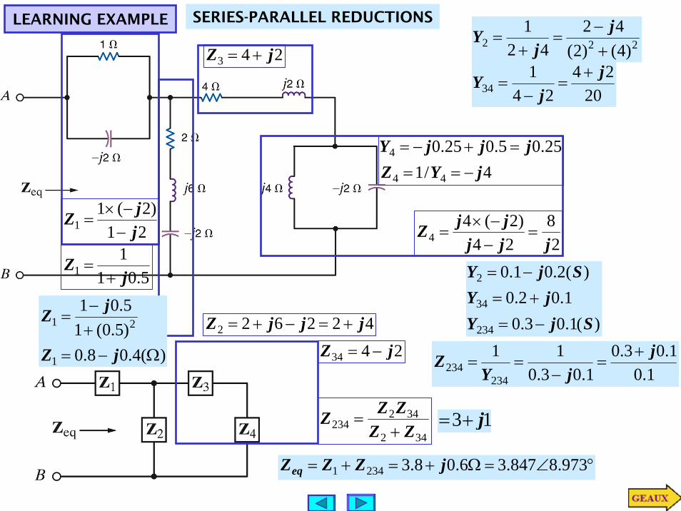
LEARNING EXAMPLE SERIES-PARALLEL REDUCTIONS

243 jZ +=

4/125.05.025.0

44

4

jYZjjjY

−===+−=

28

24)2(4

4 jjjjjZ =

−−×

=

422622 jjjZ +=−+=

21)2(1

1 jjZ

−−×

=

5.011

1 jZ

+=

2434 jZ −=

342

342234 ZZ

ZZZ+

= 13 j+=

)(1.03.01.02.0

)(2.01.0

234

34

2

SjYjY

SjY

−=+=−=

)(4.08.0)5.0(15.01

1

21

Ω−=+−

=

jZ

jZ

°∠=Ω+=+= 973.8847.36.08.32341 jZZZeq

222 )4()2(42

421

+−

=+

=j

jY

2024

241

34j

jY +

=−

=

1.01.03.0

1.03.011

234234

jjY

Z +=

−==

LEARNING EXTENSION TZIMPEDANCETHEFIND

24464

1

1

jZjjZ

+=−+=

222 jZ +=

°∠=→ 565.26472.4)( 1ZPR°−∠= 565.26224.01Y

°∠=→ 45828.2)( 2ZPR°−∠= 45354.02Y

100.0200.0)( 1 jYRP −=→

250.0250.0)( 2 jYRP −=→

35.045.02112 jYYY −=+=°−∠=→ 875.37570.0)( 12YPR

°∠= 875.37754.112Z077.1384.1)( 12 jZRP +=→

222 )2()2(22

221

+−

=+

=j

jY

077.1383.3)1077384.1(2 jjZT +=++=221 )2()4(

2424

1+−

=+

=j

jY

325.035.045.0

35.045.011

1212

jjY

Z +=

−==

1212

2112

1Y

Z

YYY

=

+=

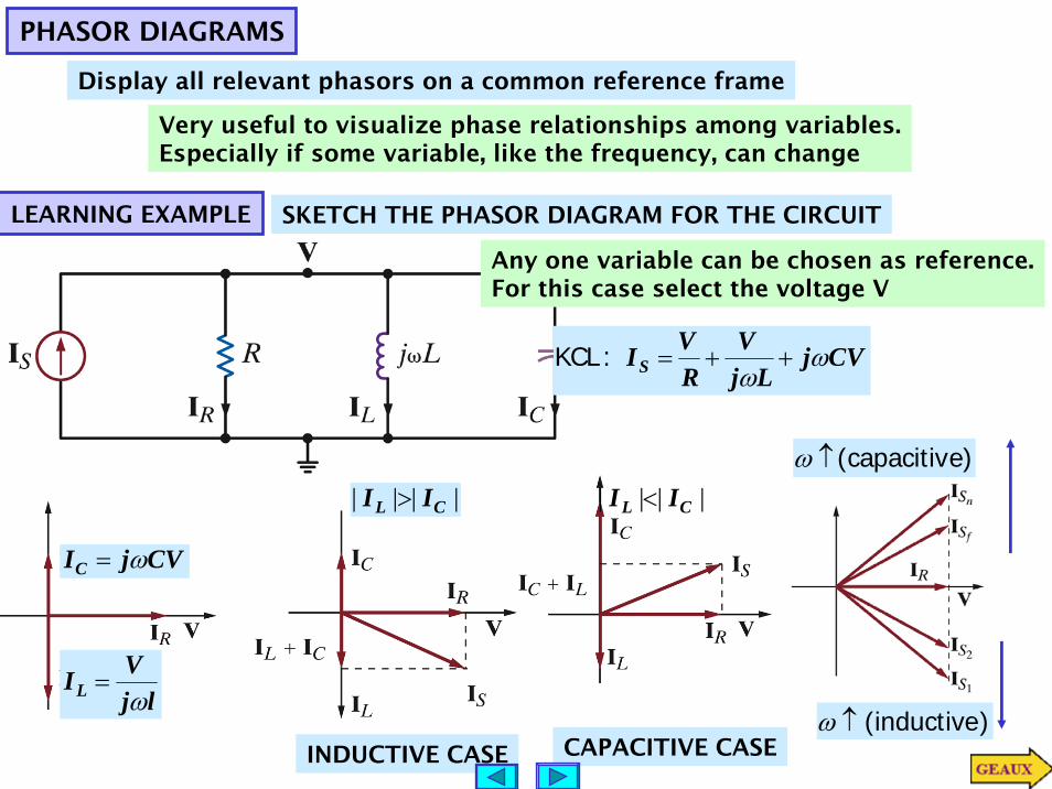
LEARNING EXAMPLE SKETCH THE PHASOR DIAGRAM FOR THE CIRCUIT

PHASOR DIAGRAMS

Display all relevant phasors on a common reference frame

Very useful to visualize phase relationships among variables.Especially if some variable, like the frequency, can change

Any one variable can be chosen as reference.For this case select the voltage V

CVjLj

VRVIS ω

ω++= :KCL

|||| CL II >

INDUCTIVE CASE

|||| CL II <

CAPACITIVE CASE

e)(capacitiv↑ω

)(inductive ↑ω

CVjIC ω=

ljVIL ω

=

LEARNING EXAMPLE DO THE PHASOR DIAGRAM FOR THE CIRCUIT

CLRS

C

L

R

VVVV

ICj

V

LIjVRIV

++=

=

==

ω

ω1

It is convenient to selectthe current as reference

1. DRAW ALL THE PHASORS

)(377 1−= sω 2. PUT KNOWN NUMERICAL VALUES

|||| RCL VVV =−

°∠= 90212SV REFERENCE WITH DIAGRAM

Read values fromdiagram!

s)(Pythagora)(4512 VVR °∠=)(453 AI °∠=∴

°−∠= 456CV

)(13518 VVL °∠=

|||| CL VV >

LEARNING BY DOING

PHASEINAREANDWHICH ATFREQUENCY THEFIND )()( titv

−

+)(tv

lineal-coarefor phasorsthei.e., )(),( tvti

RILIjICj

V ++= ωω1

C

L

R

I

LIjω

ICjω

1 RI

RILIjICj

V ++= ωω1

PHASOR DIAGRAM

01=+

CjLjIV

ωω iff lineal-co are and

LC12 =⇒ω

)/(10162.3101010

1 4963

2 srad×=⇒=×

= −− ωω

Hzf 310033.52

×==πω

Notice that I waschosen as reference

LEARNING EXTENSION Draw a phasor diagram illustrating all voltages and currents

°∠°−∠

°−∠=

−−

= 454435.63472.4

90442

41 I

jjI

)(435.18578.31 AI °∠=

Currentdivider

°∠°−∠

°∠=

−= 454

435.63472.402

421

2 Ij

I

°∠= 435.108789.12I 12 III −=thanSimpler

)(435.18156.72 1 VIV °∠==

DRAW PHASORS. ALL AREKNOWN. NO NEED TO SELECT A REFERENCE

BASIC ANALYSIS USING KIRCHHOFF’S LAWS

PROBLEM SOLVING STRATEGY

For relatively simple circuits use

divider voltageandCurrent KVL KCL AND

and combiningfor rules The i.e.,analysis;for AClawsOhm'YZ

IZV =

For more complex circuits use

PSPICEMATLAB

theorems sNorton' and sThevenin'tiontransforma Source

ionSuperpositanalysis LoopanalysisNode

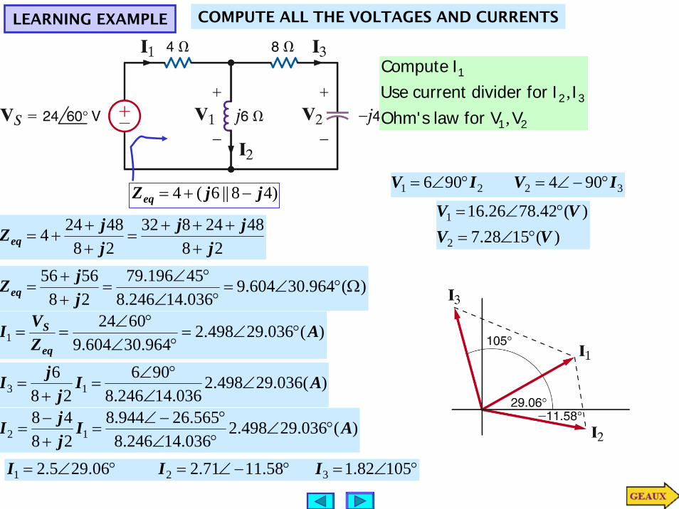
LEARNING EXAMPLE COMPUTE ALL THE VOLTAGES AND CURRENTS

)48||6(4 jjZeq −+=

284824832

2848244

jjj

jjZeq +

+++=

++

+=

)(964.30604.9036.14246.845196.79

285656

Ω°∠=°∠

°∠=

++

=jjZeq

)(036.29498.2964.30604.9

60241 A

ZVI

eq

S °∠=°∠

°∠==

)(036.29498.2036.14246.8

90628

613 AI

jjI ∠

∠°∠

=+

=

)(036.29498.2036.14246.8565.26944.8

2848

12 AIjjI °∠

°∠°−∠

=+−

=

3221 904906 IVIV °−∠=°∠=

°∠=°−∠=°∠= 10582.158.1171.206.295.2 321 III

)(1528.7)(42.7826.16

2

1

VVVV

°∠=°∠=

21

32

1

Vfor V law sOhm'IIfor divider current Use

ICompute

,,

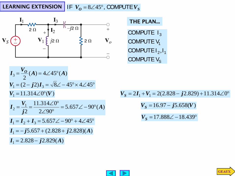
LEARNING EXTENSION SO VV COMPUTE, IF °∠= 458

S

12

1

3

VCOMPUTEII COMPUTE

VCOMPUTEI COMPUTE

,

THE PLAN...

)(454)(23 AAVI O °∠==

°∠×°−∠=−= 454458)22( 31 IjV)(0314.111 VV °∠=

)(90657.5902

0314.1121

2 AjVI °−∠=

°∠°∠

==

°∠+°−∠=+= 45490657.5321 III

))(828.2828.2(657.51 AjjI ++−=

)(829.2828.21 AjI −=

°∠+−=+= 0314.11)829.2828.2(22 11 jVIVS

)(658.597.16 VjVS −=

°−∠= 439.18888.17SV

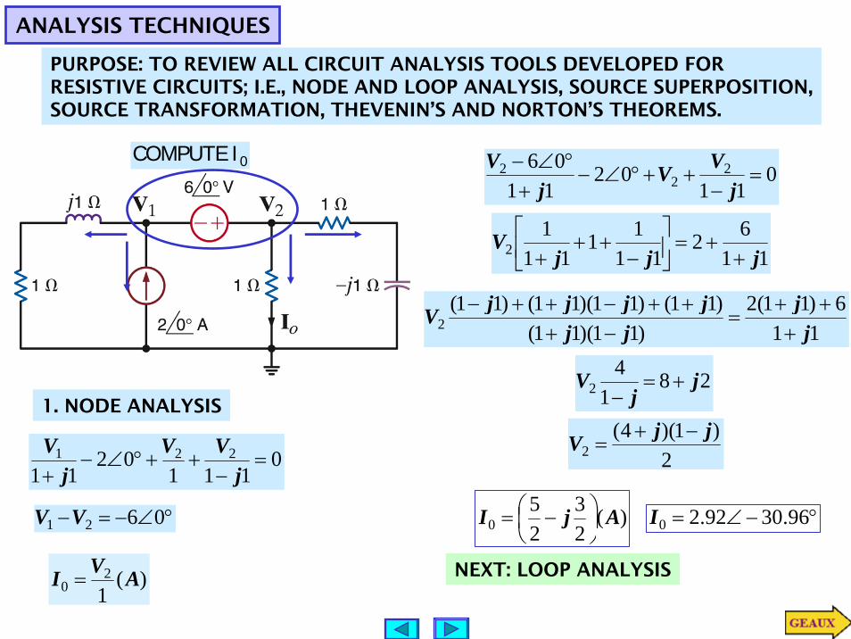
ANALYSIS TECHNIQUES

PURPOSE: TO REVIEW ALL CIRCUIT ANALYSIS TOOLS DEVELOPED FOR RESISTIVE CIRCUITS; I.E., NODE AND LOOP ANALYSIS, SOURCE SUPERPOSITION,SOURCE TRANSFORMATION, THEVENIN’S AND NORTON’S THEOREMS.

0ICOMPUTE

1. NODE ANALYSIS

0111

0211

221 =−

++°∠−+ j

VVj

V

°∠−=− 0621 VV

)(12

0 AVI =

011

021106 2

22 =

−++°∠−

+°∠−

jVV

jV

1162

1111

111

2 jjjV

++=⎥

⎦

⎤⎢⎣

⎡−

+++

116)11(2

)11)(11()11()11)(11()11(

2 jj

jjjjjjV

+++

=−+

++−++−

281

42 j

jV +=

−

2)1)(4(

2jjV −+

=

NEXT: LOOP ANALYSIS

)(23

25

0 AjI ⎟⎠⎞

⎜⎝⎛ −= °−∠= 96.3092.20I

2. LOOP ANALYSIS

SOURCE IS NOT SHARED AND Io IS DEFINED BY ONE LOOP CURRENT

°∠−= 021I :1 LOOP

0))(1(06))(1( 3221 =+−+°∠−++ IIjIIj:2 LOOP

3I FIND MUST

30 II −=

0))(1( 332 =++− IIIj :3 LOOP

)2)(1(6)1(2 32 −+−=−+ jIjI

0)2()1( 32 =−+− IjIj )2(/*)1(/*

−− j

( ) )28)(1()2(2)1( 32 jjIjj +−=−−−

4610

3 −−

=jI )(

23

25

0 AjI +−=

ONE COULD ALSO USE THE SUPERMESHTECHNIQUE

2I

0)1()(0)(06)1(

02

323

321

21

=−+−=−+°∠++

°∠−=−

IjIIIIIj

II

:3 MESH :SUPERMESH:CONSTRAINT

320 III −=

NEXT: SOURCE SUPERPOSITION

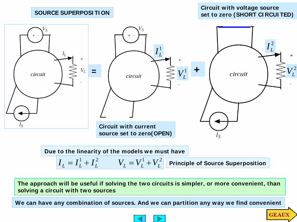
Circuit with currentsource set to zero(OPEN)

1LI

1LV

Circuit with voltage sourceset to zero (SHORT CIRCUITED)

2LI

2LV

SOURCE SUPERPOSITION

= +

The approach will be useful if solving the two circuits is simpler, or more convenient, than solving a circuit with two sources

Due to the linearity of the models we must have2121

LLLLLL VVVIII +=+= Principle of Source Superposition

We can have any combination of sources. And we can partition any way we find convenient

3. SOURCE SUPERPOSITION

1)1()1(

)1)(1()1(||)1(' =−−+−+

=−+=jj

jjjjZ

)(01'0 AI °∠=

)1(||1" jZ −=

)(061"

""

1 VjZ

ZV °∠++

= )(061"

""0 A

jZZI °∠

++=

)(61

21

21

"0 A

jjj

jj

I++

−−

−−

=6

3)1(1"

0 jjjI++−

−=

)(46

46"

0 AjI −=

)(23

25"

0'00 AjIII ⎟

⎠⎞

⎜⎝⎛ −=+=

NEXT: SOURCE TRANSFORMATION

"Z

"0I COMPUTE TO

TIONTRANSFORMASOURCEUSECOULD

Source transformation is a good tool to reduce complexity in a circuit ...

WHEN IT CAN BE APPLIED!!

Source Transformationcan be used to determine the Thevenin or Norton Equivalent...

BUT THERE MAY BE MORE EFFICIENT TECHNIQUES

“ideal sources” are not good models for real behavior of sources

A real battery does not produce infinite current when short-circuited

+-

Improved modelfor voltage source

Improved modelfor current source

SVVR

SI

IRa

b

a

b SS

IV

RIVRRR

===

WHEN SEQUIVALENT AREMODELS THEVZ

IZS S

I VZI V

Z Z Z=

= =

LINEAR CIRCUITMay contain

independent anddependent sources

with their controllingvariablesPART A

LINEAR CIRCUITMay contain

independent anddependent sources

with their controllingvariablesPART B

a

b_Ov+

i

THEVENIN’S EQUIVALENCE THEOREM

LINEAR CIRCUIT

PART B

a

b_Ov+

i

−+

THR

THv

PART A

Thevenin Equivalent Circuit

for PART A

Resistance Equivalent Thevenin SourceEquivalent Thevenin

TH

TH

Rv Impedance

THZ

Phasor

LINEAR CIRCUITMay contain

independent anddependent sources

with their controllingvariablesPART A

LINEAR CIRCUITMay contain

independent anddependent sources

with their controllingvariablesPART B

a

b_Ov+

i

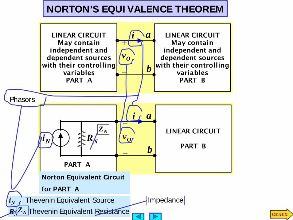
NORTON’S EQUIVALENCE THEOREM

Resistance Equivalent Thevenin SourceEquivalent Thevenin

N

N

Ri

LINEAR CIRCUIT

PART B

a

b_Ov+

i

NRNi

PART A

Norton Equivalent Circuit

for PART A

Phasors

Impedance

NZ

NZ

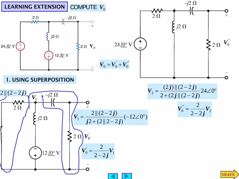
LEARNING EXTENSION 0V COMPUTE

1. USING SUPERPOSITION

'0V

"0V

"0

'00 VVV +=

1V

)012()22||2(2

)22(||21 °∠−

−+−

=jj

jV

1'

0 222 V

jV

−=

2 V

°∠−+−

= 024)22(||2(2

)22(||)2(2 jj

jjV

2"0 22

2 Vj

V−

=

)22(||2 j−

2. USE SOURCE TRANSFORMATION

°∠012 Ω2 °−∠ 906

Ω− 2j

Ω2

−

+

0V1I

Ω2j

2||2 jZ =

eqIZ

j2−

2−

+

0V1I

eqIjZ

ZI221 −+

=

10 2IV =

jIeq 612906012 +=°−∠−°∠=

USE NORTON’S THEOREM

2||2 jZTH =

SCI

°∠012

°−∠− 906

SCI THZ

2j−

2−

+

0V1I

SCTH

TH IjZ

ZI221 −+

=

10 2IV =