AEDC-TR-81-~22

Accelerated Convergence of Structured BandedX • Systems Using Constrained Corrections

Karl KneileSverdrup Technology, Inc.

= December 1981

Final Heport for Period October 1980 - August 1981

DTIC•LEETEa

DEC 221981

Approved for public release; distribution unlimited.

I ____

ARNOLD ENGINEERING DEVELOPMENT CENTERARNOLD AIR FORCE STATION, TENNESSEE

AIR FORCE SYSTEMS CO VIMANDUNITED STATES AIR FORCE

81 12 23 153

----- -~. 1

-A

NOTICES

When U. S. Government drawings specif'cations, or other data Ate uwd for any purpose otherthan a definitely related Gomntment procuremnt operation, the Govemment thereby incurs noresponsibility nor any obliation whatsoever, and the fact that the Government may have "

formulated, fumshd oat m any way supplid the said drawrip. specifications, or other " is gnot to be rgarded by implicaUon or otherwise, or in any mainei licensing the holder or iltyother perw.o or corporation, or conveyig any rights or permission to manufacture, use, or ,ilIany patented invention that may in any way be related thereto.

Qualified users •ay obtain copies of this report from the Defense Techdinlc inhnlrnation Center

Refetrene to named commercul products in this report me not to be cotudr-red in an) sense-is ,n endorse:ent of the product by the United StAtes Air ForCe of the GoWerarne(t.

~1

7" Mpxn has been reveie~l L.y th Offia of PlabdcAt &L- (PA) andi o •icuasv le to e U ]tNpAbIa, mtrTechlucagl forqlnfMUM~ntzas Servce (MWOl~. At NM-LS it wili be avallable te •bc general

APPROVAL. STATEMENT i

LffTpu I- CLpSŽruVtui

kpprovec 1o1 publicaiiorv

FO-* Tell cCMM.cINILIý

I

-J, -

IFqpur Ic• Uper~auonm

4- - -*.--.~- - .- -

"UNCLASSIFIEDSECURITY CLASSIFICATION OF THIS PAGE (When OstafDrntered)i 4

REPORT DOCUMENTATION PAGE READ INSTRUCTIONSBEFORE COMPLETING FORM

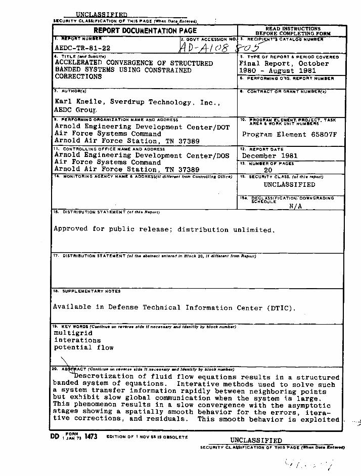
-IREPORT-NUMB|ER 1OVT ACCESSION NO. 3 RECOPIE.T's CATALOG NUMBERAEDC-TR-81-22 ý D-A-/08 .K4. TITLE (and Subtitle) S. TYPE OF REPORT & PERIOD COVEREDACCELERATED CONVERGENCE OF STRUCTURED Final Report, OctoberBANDED SYSTEMS USING CONSTRAINED 1980 - August 1981CORRECTIONS 6. PERFORMING 00. REPORT NUMBER

7. AUTHOR(s) S. CONTRACT OR GRANT NUMBER(s)

Karl Kneile, Sverdrup Technology, Inc.,AEDC Group,9. PERFORMING ORGANIZATION NAME AND ADDRESS 10. PROGRAM ELEMENT. PROJECT. TASK

AREA &WORK UNIT NUMBERSArnold Engineering Development Center/DOTAir Force Systems Command Program Element 65807FArnold Air Force Station, TN 37389II. CONTROLLING OFFICE NAME AND ADDRESS 12. REPORT DATEArnold Engineering Development Center/DOS December 1981Air Force Systems Command 13. NUMBER OF PAGES

Arnold Air Force Station, TN 37389 2014. MONITORING AGENCY NAME & ADDRESS(If' different from Controlling Office) IS. SECURITY CLASS. (of this report)

UNCLASSIFIEDISm. DECLASSIFICATIONDOWNGRADING

SCHEDULEt_ _N/A

16. DISTRIBUTION STAI EMENT (of this Report)

Approved for public release; distribution unlimited.

17. DISTRIBUTION STATEMENT (of the ebstrect entered In Block 20, If different from Report)

IS. SUPPLEMENTARY NOTES

Available in Defense Technical Information Center (DTIC).

19. KEY WORDS (Continue on reverse side if nec'essry amd Identify by block number)multigridinterationspotential flow

20. AB&I"q ACT (Conthue on reverse side It necesnary ind Identify by block number)-Descretization of fluid flow equations results in a structured

banded system of equations. Interative methods used to solve sucha system transfer information rapidly between neighboring pointsbut exhibit slow global communication when the system is large.This phenomenon results in a slow convergence with the asymptoticstages showing a spatially smooth behavior for the errors, itera-tive corrections, and residuals. This smooth behavior is exploited

FORM

DD I JAN 73 1473 EDITION OF I NOV 65 IS OBSOLETE UNCLASSIFIED

SECURITY CLASSIFICATION OF THIS PAGE ('When Data Ented)

Ii] 4

UNCLASSIFIEDSECURITY CLASSIFICATION OP THIS PAO(r••amn Dbda gnteftd)

20. ABSTRACT, Concluded.

ýy approximating the error and corrections with an interpolationover a selected subset of the grid. A variational form is usedto compress the original system of equations into a smaller system.This compression is repeated through several levels of grid sizesto obtain a dramatic improvement in convergence rate. A relaxationparameter is dynamically calculated at each step with a negligibleincrease in computational effort. Although the method was devel- I.oped for solving full potential flow using a variational principle,it is applicable to other problems with the structured bandedproperty.

ILr

fi.

UNCLASSIFIEDSECURITY CLASSIPICATIOW1 OP TUO P•,G(~hen Daoe EntereJ)

L *

AEDC-TR-41-22

fI

PREFACE

The work reported herein was conducted by the Arnold Engineering DevelopmentCenter (AEDC), Air Force Systems Command (AFSC). The Air Force project manager wasDr. Keith Kushman, AEDC/DOT. The results of the research were obtained by SverdrupTechnology, Inc., AEDC Group, operating contractor for propulsion testing at the AEDC,AFSC, Arnold Air Force Station, Tennessee, under Project Number P32A-AH1. The

manuscript was submitted for publication on September 14, 1981.

Aooession For

DTIC TABUnannounced ElJtkstification

By -Distribution/Availability Codes

Avail and/orDist Special

,4.

F-1

ii i -

I!

I ...L " .::2... .. i • - i HI[, ,

ARDC-IR41 -22J

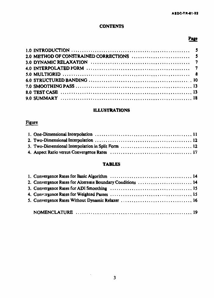
CONTENTS

1.0 INTRODUCTION .................................................. 52.0 METHOD OF CONSTRAINED CORRECTIONS..........................S53.0 DYNAMIC RELAXATION ......................................... 74.0 INTERPOLATED FORM ............................................ 75.0 MULTIGRID ...................................................... 86.0 STRUCTURED BANDING ..................................... .. .107.0 SMOOTHING PASS................................................. 138.0 TEST CASE ....................................................... 139.0 SUMMARY ....................................................... 18

ILLUSTRATIONS

Figure

1. One-Dimensional Interpolation......................................... 112. Two-Dimensional Interpolation......................................... 12 j3. Two-Dimensional Interpolation in Split Form .............................. 124. Aspect Ratio versus Convergence Rates................................... 17

TABLES j1. Convergence Rates for Basic Algorithm................................... 142. Convergence Rates for Alternate Boundary Conditions....................... 143. Convergence Rates for ADI Smoothing................................... 15A4. Convzrgence Rates for Weighted Passes................................... 155. Convergence Rates Without Dynamic Relaxer .............................. 16

NOMENCLATURE................................................. 19

3i

AEDC.TR41-22

1.0 INTRODUCTION

The purpose of this report is to describe an efficient Iteratlve method for solving astructured banded system of equations. Although the method was developed for a fullpotential flow program, it wiM be presented in general terms applicable to a wide range ofproblems. The central Issue here is the solution of a largv linear system of equations. Thelinear system may arise directly in the problem or may result from an iteration in a nonlinearproblem. For large two-dimensional (2-D) and three-dimen~ional (3-D) applications, thislinear system becomes increasingly expensive to solve directly. As a result, efficient iterativemethods have become attractive for large problems. In the nonlinear cases, these iterationsmay be effectively merged to Improve convergence rates.

Conventional iterative methods (Jacobi, Gauss-Seidel, ADI, etc.) rapidly rm .71) a statewhere convergence rates are limited by the large eigenvalues of the system. Thisphenomenon is especially restrictive for large problems. Various approaches have been triedto accelerate convergence. Relaxation made some modest gains, but obtaining an optimumor near-optimum parameter was sometimes difficult. Others have tried more elaborateiterative methods [incomplete Crout, strongly implicit procedure (SIP), and SIP/conjugategradient) with considerable success. However, the most dramatic improvements have beenseen recently with the revival of multigrid concepts.

The method presented in this report uses a basic iteration step (incomplete Croutreduction), a dynamic relation step, and a multigrid concept of constraining iterativecorrections.

2.0 METHOD OF CONSTRAINED CORRECTIONS

The method of constrained corrections uses a variational form of the problem. Thisvariational form may be part of the problem definition or may be artificialiy created tisdescribed later.

The discretized variational form may be represented as L(O), where L is a scalar functionof the n component vector #. The components of 0 are obtained by solving the nsimultaneous equations

F = 0 (1)

An iterative procedure (Newton's) for solving this system is as follows:

A AS = r (2)

5

AEOC-T-t1-22.

where

8.•i+l - f•i'

*-F

andA - ai•/aol, akla/,,l,

For linear problems the iteration procem is trivial and ends with the first iteration.

If a variational principle is not part of the problem, one can define

L* (8) - 48TA8 8T r (3)

and use

80*/a8 - 0 (4)

as the variational form. This is equivalent, both here and in later consilierations, to using

coupled with Newton's method if (5) is nonlinear in 6. The method of constrainedcorrections defines 6 as

8 =Ck (6)

The vector k has p < n comnonents. The matrix C prescribes each component of 6 as alinear combination of the components of k. It will be assumed that C is of rank p (i.e., thecolumns of C are linearly independent). This is equivalent to imposing (n - p) linearcombinations of the components of 6 as zero. That is,

C * 8 .0 (7)

where C* is an (n -p) x n matrix. It is more convenient to use these constraints in the form ofEq. (6).

Substitution of (6) into the variational form results in the system of equations

CTAC k = CTr (8)for the unknown k vector. The 6 vector is then obtained from (6). With judicious selectionsof C and k, the convergence rate can be substantially improved.

6

[iI,• • Im •,•, t .• •! ' l .. _ _• • • •t,, l•_ e '

AIOC.TA41422

3.0 DYNAMIC RELAXATION j

Consider sdaln the basic linear system, (2). When using an iterative method, one obtains jan approximate 6 denoted by 6a. By letting C in (6) be the vector 6a, the relaxationparameter, k, is then given by

k 85Tr/8T/&j (9)a a a

The iteration then takes the form

0i+ 1 0 ka (10)

The residual r in (9) is the original residual vector using *h and is not obtained frJin using*i + 6,. •

4.0 INTERPOLATED FORM

It is easier to describe this form for one-dimensional problems. The components of areassociated with a positional value along this dimension. As mentioned earlier, conventionaliterative methods rapidly reach an asymptotic convergence limited by the larger eigenvalues.It is well known that these iterations rapidly remove the smaller wavelength components,leaving the smooth, longer wavelength components. Conventional multigrid methodsexploit this smoothness to justify using a coarse grid optrator. This paper will also takeadvantage of this smoothing property, but will direct emphasis toward the smoothness of thecorrection vector, 6. A basis vector, 6b, is selected. The correction vector is then constrainedto the following form:

~ L--b (11)

In actual practice the components of 6 b &re interspersed within 6, and the rows of B aremerged with the rows of the identity matrix. The above representation (separated I and B)will be used to simplify notation. For this special case the constraints take the form

C 8 [B:-IjS8O0(12)

The B matrix represents interpolation coefficients for the nonbasis components.Solutions of

CACb 8 CTr (13)

7

A IOC-IR41.I122

coupled with (11) will then "solve the original problem" subject to the constraints. The

effectiveness of this constrained form depends upon the form of interpolation used, the

smoothness of 8, and the difficulty in solving the new system, (13). The smiler thedimension of 6, 'he simpler system (13) is to solve. However, more iterations are needed to

precondition the smoothness required for effective interpolation.

The dynamic relaxation step described in the previous section can be used to improve

overall convergence. The relaxation factor may be calculated using the basis &, as follows:

k 8 T(C Tr)/8 (CTAC)b (14)

5.0 MULTIGRID

The constrained corrections method described in the previous section can be easily

"adapted to a multigrid concept. A nested sequence of basis vectors is defined by

a r-iC i - 1,2, ... , m

C (15)

where be represents the original fine grid and 5m the coarsest level with the fewest

components. The B% values are interpolation coefficients from the ith level to the (i - I) level.

The above interpolations may be combined to form

80 StDi 81

D1 MCI C2 ... C1 i %,Di Ct (16)

I, The constrained system ef equations is

D T ADi T D T (17)

These equations easily lend themselves to the following iterative algorithm.

A smoothing pass is made on the fine grid system.

Ab - r (8

8

Li

AROC-TR41-22

The 4 vector is updated by (10), whereby (18) now represents the next Iterative pass. Acompression step is taken to obtain the system

A1 l 1 - (19)

where IA3 - DiTAD,

and

A smoothing pass is now made on this system. The 4 vector is again updated, and the nextiterative pass is taken at the second level,

A, r2 (20)

where

A2 2AD

andr2 D2r

The process is repeated down through the coarsest level.

The preceding describes a multigrid cycle. This cycle is repeated until sufficient

convergence is obtained. Many variations of the above algorithm are possible. A few ofthese are compared in Section 8.0.

A computational advantage can be obtained from the nesting or recursive definitions ofthe Di. The next level system can be calculated directly from the current level,

Ai 1 =CTA Ci i+1 i 1i +1

Tr1+ iC1+ir

It is not necessary to calculate the updated residuals at the fine grid level. They may becalculated at the current ith level and then compressed down one level.

9

i1

AEDC.TR4i -22

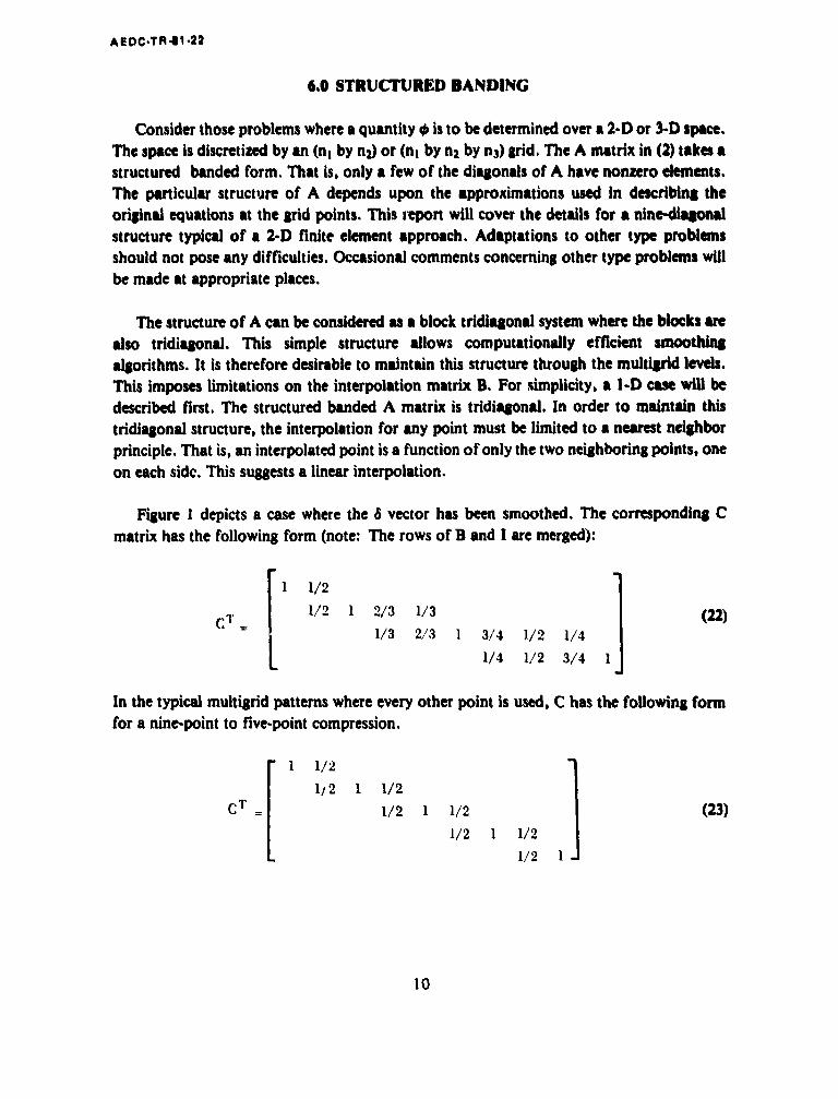
6.0 STRUCTURED BANDING

Consider those problems where a quantity 0 is to be determined over a 2-D or 3-D space.The space is discretized by an (n, by n2) or (n, by n2 by n3) grid. The A matrix in (2) takes astructured banded form. That is, only a few of the diagonals of A have nonzero elements.The particular structure of A depends upon the approximations used in describing theoriginal equations at the grid points. This report will cover the details for a nine-diagonalstructure typical of a 2-D finite element approach. Adaptations to other type problemsshould not pose any difficulties. Occasional comments concerning other type problems willbe made at appropriate places.

The structure of A can be considered as a block tridiagonal system where the blocks arealso tridiagonal. This simple structure allows computationally efficient smoothingalgorithms. It is therefore desirable to maintain this structure through the multigrid levels.This imposes limitations on the interpolation matrix B. For .Implicity, a I.-D case will bedescribed first. The structured banded A matrix is tridiagonal. In order to maintain thistridiagonal structure, the interpolation for any point must be limited to a nearest neighborprinciple. That is, an interpolated point is a function of only the two neighboring points, oneon each side. This suggests a linear interpolation.

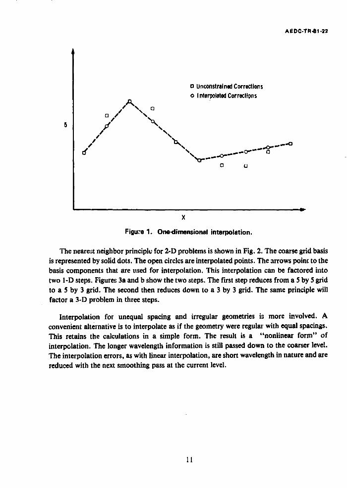
Figure I depicts a case where the 6 vector has been smoothed. The corresponding Cmatrix has the following form (note: The rows of B and I are merged):

SI 1 /2

1/2 1 2/3 1/3cl = T (22)1/3 2/3 1 3/4 1/2 1/4

1/4 1/2 3/4 1

In the typical multigrid patterns where every other point is used, C has the following formfor a nine-point to five-point compression.

11/27t 1/2 1 1/2

cT[ 1/2 1/2 (23)

1/2 1 1/2

1/2 1

10

AEDC-TR.S1.22

o Unconstrained Corrections0 Interpolated Corrections

0/0

/X

6iu- .Oedmninlitroain

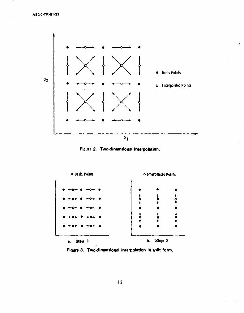
Th narstnighof rnil o - rbesi honi i.2 h oregiai

basiscompoentsFhat ure usd.o interpolation.ahi interpolation. cnb atrdit

two Il-D steps. Figures 3a and b show the two steps. The first step reduces from a 5 by 5 gridto a 5 by 3 grid. The second then reduces down to a 3 by 3 grid. The same principle willfactor a 3-D problem in three steps.

Interpolation for unequal spacing and irregular geometries is more involved. Aconvenient alternative is to interpolate as if the geometry were regular with equal spacings.This retains the calculations in a simple form. The result is a "nonlinear form" ofinterpolation. The longer wavelength information is still passed down to the coarser level..The interpolation errors, as with linear interpolation, are short wavelength in nature and arereduced with the next smoothing pass at the current level.

AEDC-TR-81-22

x * Basis Points

x 2 i

0 Interpolated Points

x i

Figure 2. Two-dimensional interpolation.

* Basis Points o Interpolated Points

: i,'-- : • II•B0 **@0. -

a. Step 1 b. Step 2

Figure 3. Two-dimensional interpolation in split form.

L 1

I

12Ii1

AEDC-TR1-8 22

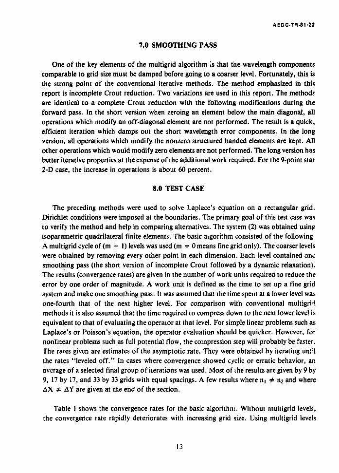
7.0 SMOOTHING PASS

One of the key elements of the multigrid algorithm is that the wavelength components

comparable to grid size must be damped before going to a coarser level. Fortunately, this isthe strong point of the conventional iterative methods. The method emphasized in thisreport is incomplete Crout reduction. Two variations are used in this report. The methodsare identical to a complete Crout reduction with the following modifications during theforward pass. In the short version when zeroing an element below the main diagonal, alloperations which modify an off-diagonal element are not performed. The result is a quick,Aefficient iteration which damps out the short wavelength error components. In the longversion, all operations which modify the nonzero structured banded elements are kept. Allother operations which would modify zero elements are not performed. The long version hasbetter iterative properties at the expense of the additional work required. For the 9-point star2-D case, the increase in operations is about 60 percent.

8.0 TEST CASE

* The preceding methods were used to solve Laplace's equation on a rectangular grid.Dirichlet conditions were imposed at the boundaries. The primary goal of this test case wasto verify the method and help in comparing alternatives. The system (2) was obtained usingisoparametric quadrilateral finite elements. The basic aigorithm consisted of the followingA multigrid cycle of (m + 1) levels was used (m = 0 means fine grid only). The coarser levelswere obtained by removing every other point in each dimension. Each level contained onesmoothing pass (the short version of incomplete Crout followed by a dynamic relaxation).The results (convergence rates) are given in the number of work units required to reduce the

error by one order of magnitude. A work unit is defined as the time to set up a fine gridsystem and make one smoothing pass. It was assumed that the time spent at a lower level wasone-fourth that of the next higher level. For comparison with conventional multigri4methods it is also assumed that the time required to compress down to the next lower level isequivalent to that of evaluating the operator at that level. For simple linear problems such asLaplace's or Poisson's equation, the operator evaluation should be quicker. However, fornonlinear problems such as full potential flow, the compression step will probably be faster.The rates given are estimates of the asymptotic rate. They were obtained by iterating unt'lthe rates "leveled off." In cases where convergence showed cyclic or erratic behavior, anavcrage of a selected final group of iterations was used. Most of the results are given by 9 by9, 17 by 17, and 33 by 33 grids with equal spacings. A few results where nj * n2 and where4X * AY are given at the end of the section.

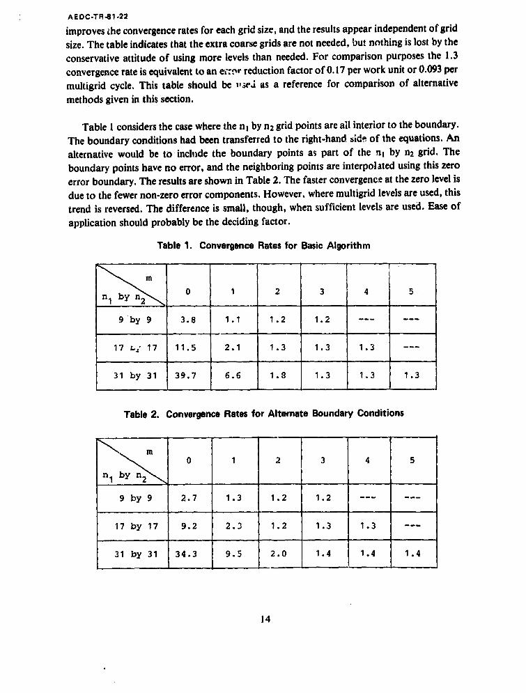
Table 1 shows the convergence rates for the basic algorithm. Without multigrid levels,the convergence rate rapidly deteriorates with increasing grid size. Using multigrid levels

13

AEDC-TR-81 -22

improves the convergence rates for each grid size, and the results appear independent of grid

size. The table indicates that the extra coarse grids are not needed, but nothing is lost by the

conservative attitude of using more levels than needed. For comparison purposes the 1.3

convergence rate is equivalent to an eý.--:r reduction factor of 0. 17 per work unit or 0.093 per Imultigrid cycle. This table should be "ve'j as a reference for comparison of alternative Imethods given in this section.

Table 1 considers the case where the nj by n2 grid points are all interior to the boundary.

The boundary conditions had been transferred to the right-hand S'd!- of the equations. An

alternative would be to include the boundary points as part of the ¶j by n2 grid. The

boundary points have no error, and the neighboring points are interpolated using this zero

error boundary. The results are shown in Table 2. The faster convergence at the zero level is

due to the fewer non-zero error components. However. where multigrid levels are used, this

trend is reversed. The difference is small, though, when sufficient levels are used. Ease of

application should probably be the deciding factor.

Table 1. Convergence Rates for Basic Algorithm

I;0 1 2 3 4 5

9 by ; 9~' 3.8 1.1 1.2 1.2 ___

34b 1 .3 9.5 120 1.4 1.43 .

14

"A EDC-TR-81-22

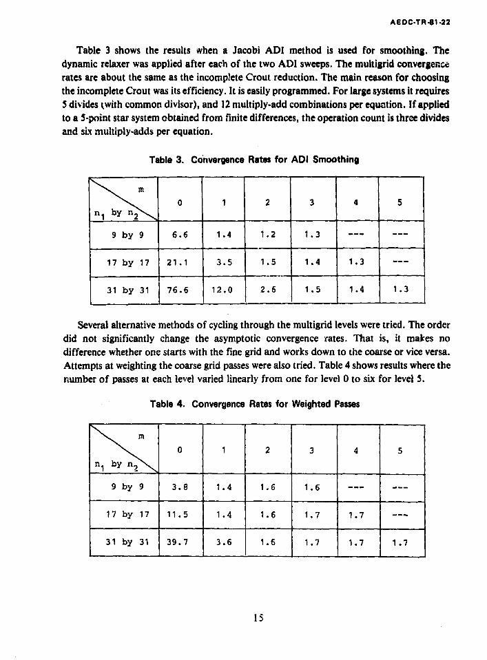
Table 3 shows the results when a Jacobi ADI method is used for smoothing. Thedynamic relaxer was applied after each of the two ADI sweeps. The multigrid convergenccjrates are about the same as the incomplete Crout reduction. The main reason for choosingthe incomplete Crout was its efficiency. It is easily programmed. For large systems it requires5 divides swith common divisor), and 12 multiply-add combinations per equntion. If appliedto a 5-point star system obtained from finite differences, the operation count is three dividesand six multiply-adds per equation.

Table 3. Convergence Rates for ADI Smoothing

m0 1 2 3 4 5

n1 by n

9 by 9 6.6 1.4 1.2 1.3

17 by 17 21.1 3.5 1.5 1.4 1.3

31 by 31 76.6 12.0 2.6 1.5 1.4 1.3

Several alternative methods of cycling through the multigrid levels were tried. The orderdid not significantly change the asymptotic convergence rates. That is, it makes no"difference whether one starts with the fine grid and works down to the coarse or vice versa.Attempts at weighting the coarse grid passes were also tried. Table 4 shows results where the

L number of passes at each level varied linearly from one for level 0 to six for level 5.

Table 4. Convergence Rates for Weighted Passes

0 1 2 3 4 5

n1 by n _ _

9 by 9 3.8 1.4 1.6 1.6

17 by 17 11.5 1.4 1.6 1.7 1.7

31 by 31 39.7 3.6 1.6 1.7 1.7 1.7

15

A EDC-TR4-1 -22

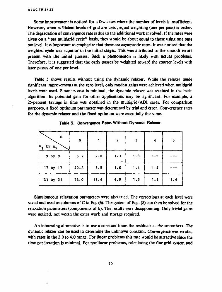
Some improvement is noticed for a few cases where the number of levels is insufficient. IHowever, when su'ficient levels of grid are used. equal weighting (one per pass) is better.The degradation of convergence rate is due to the additional work involved. If the rates weregiven on a "per multigrid cycle" basis, they 'would be about equal to those using one passper level. It Is important to emphasize that these are asymptotic rates. It was noticed that theweighted cycle was superior in the initial stages. This was attributed to the smooth errorspresent with the initial guesses. Such a phenomenon is likely with actual problems.Therefore, it is suggested that the early passes be weighted toward the coarser levels withlater passes of one per level.

Table 5 shows results without using the dynamic relaxer. While the relaxer madesignificant improvements at the zero level, only modest gains were achieved when multigridlevels were used. Since its cost is minimal, the dynamic relaxer was retained in the basicalgorithm. Its potential gain for other applications may be significant. For example, a25-percent savings in time was obtained in the multigrid/ADI cases. For comparisonpurposes, a fixed optimium parameter was determined by trial and error. Convergence rates

for the dynamic relaxer and the fixed optimum were essentially the same.

Table 5. Convergence Rates Without Dynamic Relaxer

0 1 2 345

n by n2

9 by 9 6.7 2.0 1.3 1.3 --

____________________________1 .6___ 1 .4_____________ ______________

17 by 17 20.8 5.5 16 14 1.4

31 by 31 73.0 18.6 4.9 1.5 1.1 1.4

Simultaneous relaxation parameters were also tried. The corrections at each level weresaved and used as columns of C in Eq. (6). The system of Eqs. (8) can then be solved for therelaxation parameters (components of k). The results were disappointing. Only trivial gainswere noticed, not worth the extra work and storage required.

An interesting alternative is to use a constant times the residuals a. +he smoothers. Thedynamic relaxer can be used to determine the unknown constant. Convergence was erratic,with rates in the 2.0 to 4.0 range. For linear problems this rate would be attractive since thetime per iteration is minimal. For nonlinear problems, calculating the fine grid system and

16

AEDC-TR41 -22

compression to coarser levels takes most of the time, and the overall rates would beconsiderably slower. A problem with this alternative is the relative scaling of each equation.

Several rectangular grids were also tried. The convergence rate for a 9 by 33 grid was inthe 1.2 to 1.3 range that was obtained for the square grids. The incomplete Crout smootheris order dependent. That is, different results are obtained depending upon whether the gridis numbered by rows or by columns. The convergence rates for the 9 by 33 grid were

essentially unaffected by the direction of node ordering. Ordering along the short dimensiongave less than a 2-percent improvement over the other dirr-:tion.

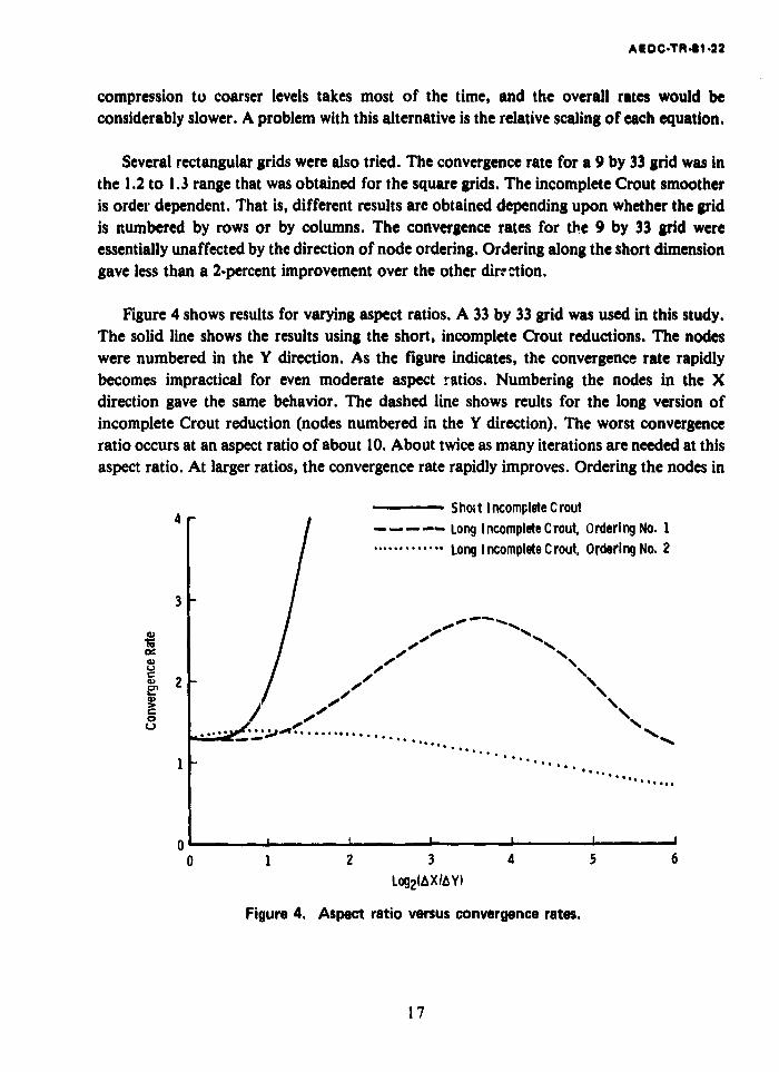
Figure 4 shows results for varying aspect ratios. A 33 by 33 grid was used in this study.The solid line shows the results using the short, incomplete Crout reductions. The nodes

were numbered in the Y direction. As the figure indicates, the convergence rate rapidlybecomes impractical for even moderate aspect ratios. Numbering the nodes in the Xdirection gave the same behavior. The dashed line shows reults for the long version ofincomplete Crout reduction (nodes numbered in the Y direction). The worst convergenceratio occurs at an aspect ratio of about 10. About twice as many iterations are needed at thisaspect ratio. At larger ratios, the convergence rate rapidly improves. Ordering the nodes in

4 Shoit Incomplete CroutLong Incomplete Crout, Ordering No. 1

.............. Long Incomplete C rout, Ordering No. 2

3

is*

*• 2-/,//*\\ 4-00)0-

o / - 0

* .

110 12 3 4 5 6Log2(AXI1AY)

Figure 4. Aspect ratio versus convergence rates.

17

S, i.1

AEDC-TR-81 -22

the X direction gives the results shown by the dotted line. Except for a small increase at thesmaller aspect ratios, this ordering gave better results. The unexpected improvement at largeaspect ratios is probably due to the regular rectangular geometry. Extrapolation of theseresults to more ,eneral geometries would be speculative. Further study is needed,particularly in the selection of the smoother.

9.0 SUMMARY

A constrained corrections algorithm was described in the previous sections. The methodwas used to solve Laplace's equation on a rectangle. A convergence rate of 1.3 fine gridwork units per decade reduction in error was obtained.

The algorithm uses a multigrid concept with the following components:

1. Incomplete Crout reduction is used to smooth the errors.

2. A dynamic relaxation parameter is used.

3. Coarse grid systems are obtained by constraining the corrections at the fine gridlevel. These constraints are In the form of simple interpolation.

The method has some drawbacks. The system of equations needs to be stored.Recalculation of the fine gr•.d at each level would increase the computational effort by a

factor approximately proportional to the number of levels used. For nonlinear problems,updating the nonlinear parts can be accomplished only at the fine grid level. Anotherdrawback occurs with the simple forms typical of finite difference methods. For example, a2-D finite difference method usually uses a 5-point rather than a 9-point star. Theinterpolation used in this paper will not maintain this 5-diagonal system, but expands to a9-diagonal system.

The main advantage of the method is the influence of the interpolation formulas. The

coarse grid systems contain not only the "average residuals," but also fine grid geometryinformation and the implied interpolation of the solution back to the fine grid. It is expectedthat this unification between the multigrid phases will prove advwntageous when generaldistorted geometries are used. The method is easy to use and does not require guesswork fordetermining parameters. Simple interpolation forms are used, producing efficient iterations.

It is the opinion of the author that the advantages will outweigh the disadvantages. A3-D full potential program is being developed using the method presented in this report.

18

AEOC-TR41-22

NOMENCLATURE

A Coefficient matrix for a linear system of equations

SAi Coefficient matrix at ith multigrid level

B Interpolation coefficient matrix

Bi Interpolation coefficient matrix from level i to level (i - 1)

C Augmented interpolation coefficient matrix

C1 Augmented interpolation coefficient matrix from level i to level (i - 1)

C* Matrix defining linear constraints implied by C

Di Interpolation coefficient matrix from level i to fine grid

F Vector defined by aL/ao4

k Vector of unknowns in constrained correction formulation

L Variational form

L* Alternate variational form

m Maximum number of levels used (m = 0 means fine grid only)

nl,n 2,n3 Number of nodes in a given direction of the grid

r Residual vector

ri Residual vector at ith level

6 Correction vector

6• Correction vector approximation

6b A basis vector used for interpolation

6i Basis vector at the ith level

41 Solution vector

i*h iteration for the solution vector

( )T Transpose operator

19

iIL~ _

-- .--------

\EDC.TR41-22

A vector composed of derivatives of L with respect to elements of

a F/f Matrix composed of derivatives of the elements of F wvith respect to elementsof 0 (The F componel ts determine rows, and the 0 components determinecolumns.)

63L/80 2 Alternate notation for 8F/8, (The matrix composed of second derivatives ofL with respect to elements )f 0.)

iI

20