accepted 1984 december 26. received 1984 … · inversion of seismic refraction data 83 gutowski...

$: Accepted 1984 December 26. Received 1984 … · Inversion of seismic refraction data 83 Gutowski & Wagner (1982) computed the plane wave decomposition using the angle of incidence$
Geophys. J. R. astr. SOC. (1985) 82,81-103

Inversion of seismic refraction data in planar dipping structure

B . Milkereit Institute f o r Geophysics, university of Kiel, Kiel, West Germany

w. D. Mooney and W. M. Kohler us Geofogical Survey, 345 Middlefield Road, Mail Stop 77, Menlo Park, CA 94025, USA

Accepted 1984 December 26. Received 1984 December 26; in original form 1984 March 21

Summary. A new method is presented for the direct inversion of seismic refraction data in dipping planar structure. Three recording geometries, each consisting of two common-shot profiles, are considered: reversed, split, and roll-along profiles. Inversion is achieved via slant stacking the common-shot wavefield to obtain a delay time-slowness (tau-p) wavefield. The tau-p curves from two shotpoints describing the critical raypath of refracted and post-critically reflected arrivals are automatically picked using coherency measurements and the two curves are jointly used to calculate velocity and dip of isovelocity lines iteratively, thereby obtaining the final two-dimensional velocity model.

This procedure has been successfully applied to synthetic seismograms calculated for a dipping structure and to field data from central California. The results indicate that direct inversion of closely-spaced refraction/wide- aperture reflection data can practically be achieved in laterally inhomogeneous structures.

Introduction

Investigations of the deep structure of the continental crust commonly utilize the seismic refraction method. Whereas the gross velocity structure of the crust is rather well determined in many regions, there has recently been an increasing effort to obtain higher resolution of the crustal structure in regions of geologic importance, such as fault zones, geothermal areas and other areas of possible exploration interest. This interest has been matched by techno- logical advances that have made it possible to deploy long (1 0 km and greater) seismic arrays with large numbers of sensors at an interstation spacing measured in tens of metres. Such profiles contain both near-vertical and wide angle reflected waves and refractions, thereby rendering obsolete the traditional distinction between ‘reflection’ and ‘refraction’ seismology. Denser sampling of the wavefield has also made possible the application of new automated data interpretation procedures to what was previously a trial and error forward modelling process.

at USG

S Libraries on A

pril 24, 2013http://gji.oxfordjournals.org/

Dow

nloaded from

http://gji.oxfordjournals.org/

82 To date. many of the new procedures have been based on the transformation of the

observed wavefield into the delay time-slowness (tau-p) domain. The most important advantage of the approach is that it provides a convenient display of the information needed to obtain velocity as a function of depth.

In this paper we continue the investigation of the travel-time inversion of tau-p transformed refraction data. We describe a new method for determining the p-tau(p) curve of principal arrivals (critical raypath) in the transformed wavefield, and demonstrate a method in which lateral variations in structure are resolved. We first describe these procedures theoretically, and then apply them to synthetic and real data.

B. Milkereit, W. D. Mooney and W. M. Kohler

Theory

Slant stacking is a procedure that transforms the entire observed wavefield @ ( T , x) in the time-distance domain into a wavefield $( tau .p) in the tau-p plane, with p being the stacking or horizontal slowness and tau the intercept time or delay time (McMechan & Ottolini 1980; Brocher & Phinney 1981a; McMechan, Clayton & Mooney 1982). The quality of the inversion of the $ (tau, p ) wavefield is directly related to the quality of the transformation of the seismic data, hence, we describe tau-p transformations in detail. In preference to integral representation, we have written equation (1) for discrete, finite aperture data as a sum over N seismograms, which is a satisfactory procedure when a sufficient number (A‘) of seismograms with dense geophone spacing is available. Slant stacking may be written:

with @(T, x): seismic true amplitude trace at distance x, and time T = tau + p x , f ( x ) : geometrical spreading correction, and x: horizontal range.

Slant stacking essentially is a summing along lines of constant ‘step out’. The method can be regarded as a generalization of velocity filtering techniques for determining arrival slowness and intercept time (Chapman 1981).

To avoid spatial aliasing at the lowest horizontal phase velocity, the geophone spacing Ax must satisfy (Stoffa etal . 1981a):

Ax Q V(min)/2f(max)

with V(min): lowest horizontal phase velocity, f(max): maximum frequency.

Therefore, the transformation ( 1 ) is restricted to high quality, densely spaced reflection and refraction data. Stoffa et al. (1981a) and Stoffa, Diebold & Buhl (1981b, 1982) applied the slant-stacking technique to marine wide-aperture CMP-data. A coherency measurement (semblance; Taner & Koehler 1969) ensures that coherent arrivals across a subarray will be stacked and transformed.

The slant stack has also been modified by a number of other authors performing a plane wave decomposition for spherical excitation; Muller (197 l), Chapman (1978,198 l ) , Phinney, Chowdhury & Frazer (1981), and Henry, Orcutt & Parker (1980) introduce a convolution operator into the simple slant-stacking algorithm. Kennett (1 98 1 ) showed the possibility of presenting the plane wave reflection coefficients in the slowness-intercept time domain as an element of an approach for a combined travel-time and amplitude inversion. Treitel,

at USG

S Libraries on A


Dow

nloaded from


Inversion of seismic refraction data 83

Gutowski & Wagner (1982) computed the plane wave decomposition using the angle of incidence (at the surface) instead of the horizontal slowness p , and applied deconvolution to the transformed seismic data.

Inversion of slant-stacked data Compared with interpreting the original T-x data, slant stacking is advantageous because it unravels triplications, and since it is a transformation of the who!e record section, there are no problems with hidden low-velocity layers. In the tau-p domain it is possible to dis- tinguish between ‘principle arrivals’ (refracted and critically reflected) and their multiples, and pre-critically and critically reflected arrivals are separated.

If there is no low-velocity zone we can construct the velocity-depth function directly from the critically reflected and refracted wavefield because this tau (p) curve of ‘principal arrivals’ is a single valued monotonic function (except in the case of extreme lateral variations). One inversion method, a tau-sum recursive inversion scheme, was described by Diebold & Stoffa (1981) for horizontal layers and a set of n observed p , tau ( p ) values:

n - 1

i = l tau (p,) = 2 C zi ( u ; ~ - p;)l12

with p , : observed apparent (horizontal) wave slowness, tau (p , ) : intercept time of pn, zi: thickness of a layer with velocity ui, ui: velocity in layer i. The tau-sum recursion for travel-time inversion solves for the layer thicknessvia the equation:

n - 2 [tau (p,)/2] - C zi(u i2 - pi)1”

(Diebold & Stoffa 1981, equation 15). We note that when a [ p , , tau (p , ) ] pair are related to post-critically reflected arrivals, the calculated layer thickness z , - = 0, i.e. a velocity discontinuity is indicated.

Clayton & McMechan (1981) presented an alternate iterative method for inversion of slant-stacked refraction data. Their method is based on the technique of wavefield continuation for which the inverted velocity-depth curve is extracted directly from the input $(tau, p ) wavefield. In their method, convergence of the inversion is determined when the

.output wavefield images the same velocity-depth function as was input to the continuation. The method has recently been applied to several field data sets by McMechan et al. ( I 982).

Carrion & Kuo (1 984) computed velocity profiles by finding the critical path (principal arrivals) in the tau-p domain with an energy approach. Since their minimization procedure is based on the use of relative energies, they do not take into account phase shifts along the p-tau ( p ) curve. Velocity-depth and density-depth profiles for horizontally stratified media were calculated from plane wave reflection coefficients in the tau-p domain by Carrion, Kuo & Stoffa (1 984).

Our approach is to determine the curve of ‘principal arrivals’ directly from the slant- stacked wavefield $ (tau, p ) . When the velocity at the surface ( u l ) is known, then p1 = l/ul, and the intercept time tau ( p l ) = 0. Due to the slant stack the wavefield is sampled in p and tau we have:

p i + < p i with pi +

tau ( p i + 1) > tau (pi), with tau (pi+ 1) = tau ( p i ) + A taui.

= p i - A p ( A p : sample interval in p ) , and

at USG

S Libraries on A


Dow

nloaded from


B. Milkereit, W. D. Mooney and W. M. Kohler 84

tau

.

a I

P

tau(p,) -- -

P3 pz P,

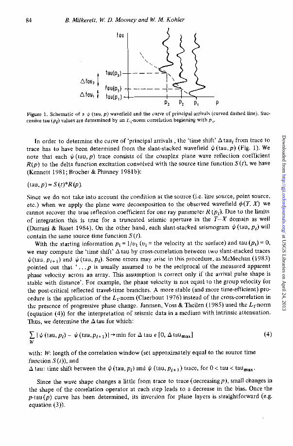
Figure 1. Schematic of a $ (tau, p ) wavefield and the curve of principal arrivals (curved dashed Line). Suc- cessive tau ( p i ) values are determined by an L,-norm correlation beginning with p , .

In order to determine the curve of ‘principal arrivals , the ‘time shift’ A taui from trace to trace has to have been determined from the slant-stacked wavefield $(tau,p) (Fig. 1). We note that each $ (tau, p ) trace consists of the complex plane wave reflection coefficient R ( p ) to the delta function excitation convolved with the source time function S ( t ) , we have (Kennett 1981; Brocher & Phinney 1981b):

(tau, P ) = s (t)*Rb).

Since we do not take into account the condition at the source (i.e. line source, point source, etc.) when we apply the plane wave decomposition to the observed wavefield $(T, X) we cannot recover the true reflection coefficient for one ray parameter R ( p i ) . Due to the limits of integration this is true for a truncated seismic aperture in the T-X domain as well (Durrani & Bisset 1984). On the other hand, each slant-stacked seismogram $ (tau, p i ) will contain the same source time function S(t) .

With the starting information p1 = l / u l ( u l = the velocity at the surface) and tau (pl) = 0, we may compute the ‘time shift’ A tau by cross-correlation between two slant-stacked traces $(tau, p i + and J / (tau, p i ) . Some errors may arise in this procedure, as McMechan (1983) pointed out that ‘ . . . p is usually assumed to be the reciprocal of the measured apparent phase velocity across an array. This assumption is correct only if the arrival pulse shape is stable with distance’. For example, the phase velocity is not equal to the group velocity for the postcritical reflected travel-time branches. A more stable (and more time-efficient) procedure is the application of the LI-norm (Claerbout 1976) instead of the cross-correlation in the presence of progressive phase change. Jannsen, Voss & Theilen (1 985) used the L l-norm (equation (4)) for the interpretation of seismic data in a medium with intrinsic attenuation. Thus, we determine the A tau for which:

IJ/(tau,pi)- J / ( t a u , p i + , ) ( + m i n f o r A t a u ~ [ O , Atau,,,] W

(4)

with: W: length of the correlation window (set approximately equal to the source time function S( t ) ) , and A tau: time shift between the li/ (tau, pi) and J / (tau, p i + trace, for 0 < tau < taumax.

Since the wave shape changes a little from trace to trace (decreasingp), small changes in the shape of the correlation operator at each step leads to a decrease in the bias. Once the p-tau ( p ) curve has been determined, its inversion for plane layers is straightforward (e.g. equation (3)).

at USG

S Libraries on A


Dow

nloaded from


i 2

3.5

Inversion of seismic refraction data

4

RANGE (KM)

2.5

6

V (kmlsec)

0 9 Y

G E O a

w

3 2

8

I-

0

0.24 0.28 0.31 0.35 0.39 0.43 0.47 0.51 0.55

P (SECIKM)

V (KM/SEC) 3.00 4.00

Figure 2. (a) Seismic record section (trace scaled by true amplitude times distance) recorded by the USGS in the Imperial Valley, southern California. Amplitude maxima on the first arrival curve are marked ‘a’ and ‘b’. (b) Slant stack of the time-distance data. Short horizontal bars indicate the p-tau ( p ) curve determined by the automatic picking procedure (see text). (c) Velocity-depth curve obtained by inverting the p-tau ( p ) curve via equation (3).

at USG

S Libraries on A


Dow

nloaded from


86

Application of the picking method

The application of this method of determining (‘picking’) the p-tau@) curve to real data is illustrated with seismic refraction data in a common-shot geometry (Fig. 2). These data were recorded by the US Geological Survey in 1979 in the Imperial Valley of southern California (Fuis et al. 1984). The seismograms are plotted in true amplitude, multiplied by distance. The first arrivals show amplitude maxima, labelled ‘a’ and ‘b’, and secondary, multiply- refracted arrivals following the first arrivals (located 0.6 s behind the first arrivals at 7 km range). This record section has been slant stacked using plane-wave decomposition.

A reliable seismic model can be obtained from the refracted and post-critically reflected wavefield when the slant stack is done for a sufficient number of equally spaced ray parameters if the length of the profile has been chosen to ensure that all ray parameters needed for inversion are within the observed data (Brocher & Phinney 1981a). Throughout this paper the transformed wavefield $ (tau,p) is sampled for 80 ray parameters. The p-tau(p) curve of principal arrivals corresponding to refracted and critical reflected arrivals has been automatically picked using the procedure described above. starting with tau ( p l ) , = 0 s,


0 0 1 2 4

RANGE (Km)

4.00 -0.00 2.00 3.00 ~ ,

7

Figure 3. Ray-theoretical synthetic seismogram calculated using the indicated velocity-depth curve (simplified from Fig. 2c). Only principle arrivals have been calculated. Plotting format as in Fig. 2(a). The amplitudes ‘a’ and ‘b’ in Fig. l(a) have been reproduced, which indicated that the p-tau@) picking procedure and the inversion work well.

at USG

S Libraries on A


Dow

nloaded from



/- 11 Y 1 0

t I

Y n

2 0

22 Figure 4. Dipping-layer velocity model used for the calculation of synthetic record sections. There are two velocity discontinuities which produce reflected phases referred to as R, and R,. respectively. The three shot points used to produce synthetic data in these geornetricies are; roll-along, split, and reversed profiles.

p1 = 0.55 s km-' (corresponding to a surficial velocity of 1.8 km s-l). The picking procedure is stable, even along portions of the wavefield where phase changes occur, for example, near p values of 0.39 and 0.28skm-' (Fig. 2b). This p-tau(p) curve has been inverted to a velocity-depth curve (Fig. 2) using equation (4). The velocity-depth function shows a high velocity gradient and two prominent velocity discontinuities at about 0.9 and 1.6 km depth. Velocities greater than 3.5 km s-' are not properly resolved due to the limited profile length. In order to evaluate the validity of the velocity-depth function obtained, synthetic seismograms were calculated for a slightly simplified velocity-depth function (Fig. 3). These seismograms were calculated using ray theory and include only the primary reflected and refracted P-waves. Comparison of Figs 2(a) and 3(a) shows that the inverted velocity-depth function provides travel times that fit the observed data. Furthermore, the synthetic seismograms show amplitude maxima at about 2.5 and 5.4km that closely match those in the observed data. This agreement indicates that the picking algorithm provides a satisfactory determination of the desired p-tau ( p ) curve of principal arrivals. Having derived a method of automatic picking of the p-tau(p) curve, we apply this algorithm to seismic data in planar dipping structure.

Extension of p-tau inversion to dipping layers Based on a geometrical formulation of the seismic travel time for refracted and critically reflected arrivals, an inversion scheme for plane dipping layers was suggested by Ocola (1972). Cunningham (1974) solved the travel-time problem for repeated single-ended refraction profiles, or 'roll-along' profiles, while Johnson (1 976) inverted split-spread refraction data. Diebold & Stoffa (1981) extended the inversion of slant-stacked seismic data to dipping layers in cases of a CMP-gather where moderate dips < 3" can be easily overlooked. They also demonstrated deformation of a p-tau ( p ) curve due to dipping layers for single shot or receiver geometry, but did not take into account amplitude information.

Following Ocola (1972) and Diebold & Stoffa (1981), the travel time T for a seismic event with an apparent wave slowness p n for a fixed source (or fixed receiver) and a stack of n layers with constant velocity ui can be written:

T ( p , ) = p,x + 1 z i [cos (ai) + cos (bi)]/ui

with p n : apparent horizontal slowness due to dip, x: horizontal range, zi: layer thickness below the shotpoint, ai, bi: angles from vertical (rays going up or down), and a, = sin-' (ul pn).

'

n - 1

i = I

at USG

S Libraries on A


Dow

nloaded from


88

After performing a slant stack for the apparent ray parameter pn, the observable delay time tau ( p n ) becomes:


n - 1

i= 1 tau ( p n ) = 2 zi [cos (ai) + cos (b i ) ] /u i . (5)

We solve equation (5) recursively for the layer thickness zi starting at the surface, where p1 = l / u l and tau(pl) = 0. The relationship of the quantities x, zi, a[ and bi are described in the Appendix.

Equation (5) provides a powerful tool for the inversion of dipping structures. We emphasize that zi, the thickness of a constant velocity layer directly below the shotpoint, is directly related to tau(pi+l), the true layer velocity ui, and the dip of the layer; it is no longer the depth of a bottoming point of a ray in a horizontally inhomogeneous medium (see Appendix).

The procedure to pick the p-tau(p) curve automatically in the tau-p domain from the slant-stacked wavefield and to invert this curve can be easily extended to dipping layers. We interpret the observed wave slowness p (used for the slant stack) as an apparent wave slowness due to dip. There are three possible inversion schemes for seismic refraction data: roll along, split spread, and reversed profile geometries.

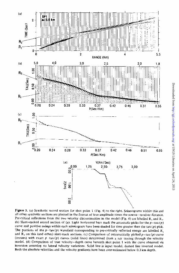
To test the inversion in laterally-varying media we have calculated ray-theoretical synthetic seismograms in a velocity model consisting of three layers, each with a positive velocity gradient (Fig. 4). (Since Diebold & Stoffa (1981) showed that the tau-sum travel-time inversion (equation 2) is perfectly adequate for zero dip velocity gradient models, we do not attempt to justify the extention of equation (5) to velocity gradients.) The interface between the second and third layers has a dip of 4.6" to the left; since the velocity is constant along the top and bottom boundaries ( e g 2.3 km s-' above the first boundary, and 2.65 km s-' below it), the velocity gradient varies laterally in the layer, decreasing from right to left. Similarly, the velocity gradient increases from right to left in the third layer. Velocities are linearly interpolated between the boundaries. The first boundary has a velocity contrast of 0.35 km s-', the second boundary of 1 .O km s-'. Synthetic seismograms have been calculated for shot points at three locations in the model (Fig. 4) in order to have data to test the three recording geometries considered. Each is described in the Appendix.

The synthetic seismogram sections were calculated using the ray theory approach of McMechan & Mooney (1980); in this method, ray paths are calculated through the medium by numerical integration of the eikonal equations (Cerveny, Molotkov & P5enEik 1977). By

. calculating complex transmission and reflection coefficients at boundaries, geometrical spreading between successive rays, and noting phase shifts or caustics, the amplitudes of geometrical rays may be obtained. The computed record section (Fig. 5a) includes refractions and pre- and post-critical reflections. The impulse response of the model has been convolved with a simple source function.

We begin the examination of the inversion for laterally-varying structures with an application of one-dimensional inversion of the synthetic data for shotpoint 1. Throughout this section we are interested in the principal tau-p curve. We note that dipping structures will cause deformation of travel-time curves in the T-X and tau-p domain, and low p values may be out of observation range for common shot gathers (i.e. in shooting downdip). There- fore we do not show low p value slant stacks. The slant-stacked section (Fig. 5b) has been automatically picked using a starting value of tau (pl) = 0, u1 = 1.8 km s-' ( p l = 0.55 s km-'). The display is normalized for the maximum in the $ (tau, p ) array. Shading has been applied to the traces for positive values greater than the picked tau value. Since no multiples or con- verted phases were computed in the synthetic section there are no phases in the tau-p

at USG

S Libraries on A


Dow

nloaded from


0

5.0 4.0

2 4

3.0 2.5 2.0

RANGE (Kin) 5.5

1 ;a

- - - 7 , 0.20 0.24 0.28 0.33 0.37 0.42 0.46 0.51 0.55

P( Sec /Kin)

I -

-~ T-- , R1,TO 1

0-L7---

O0.20 0.24 0.28 0.33 0.37 0.42 0.46 0.51 0.55 P( Sec/ Km)

(d) V(Km/Secl 0.00

T I

1 ;25

r0.J 0 0

Figure 5. (a) Synthetic record section for shot point 1 (Fig. 4) to the right. Seismograms within this and all other synthetic sections are plotted in the format of true amplitude times the source-receiver distance. Precritical reflections from the two velocity discontinuities in the model (Fig. 4) are labelled R, and R,. (b) Slant-stacked record section of (a). Light horizontal bars mark the automatic picks for the p-tau ( p ) curve and positive swings within each seismogram have been shaded for time greater than the tau ( p ) pick. The portions of the p-tau (p) wavefield corresponding to pre-critically reflected energy are labelled R , and R , on this (and other) slant-stack sections. (c) Comparison of automatically picked p-tau ( p ) curve (crosses) with exact p-tau ( p ) curves (solid lines) determined from a ray tracing through the velocity model. (d) Comparison of true velocity-depth curve beneath shot point 1 with the curve obtained via inversion assuming no lateral velocity variations. Solid line is input model, dashed line inverted model. Both the absolute velocities and the velocity gradients have been over-estimated below 0.3 km depth.

at USG

S Libraries on A


Dow

nloaded from


90

plane for delay times greater than the picked curve; this makes the p-tau section appear much simpler than the corresponding section for real data (Fig. 2). Clear phases off the principal branch of the p -tau curve are the two pre-critical reflections labelled R and R2.

The accuracy of the automatic picking algorithm in this case can be easily assessed: the travel-time response of the model (shotpoint 1) has been transformed into a p-tau curve and is compared with the picked value (Fig. Sc). The agreement is excellent in most areas. The largest discrepancy occurs near p = 0.37 s km-' where, due to post-critical reflections, phase changes occur in the

The p-tau (p) curve has been inverted to a velocity-depth curve using the one-dimensional formula (equation 3). The result (Fig. 5d), when compared with the model velocity-depth function beneath the shotpoint, nearly correctly estimates the depths of the layer boundaries, but clearly over-estimates the velocity gradients below the first boundary (0.3 km depth). In addition, the first-order discontinuity at the second boundary has been modelled as a high gradient zone. These discrepancies between a flat layer interpretation and the dipping layer model motivated the application of the inversion method (Appendix) that will correctly model structures with dips.

B. Milkereit, U! D. Mooney and W. M. Kohler

(tau, p) wavefield.

Inversion in laterally-varying media

(1) R O L L - A L O N G G E O M E T R Y

We first apply the inversion formulae (Appendix) to seismic refraction/wide-aperture reflection data in a roll-along geometry. The synthetic seismograms (Fig. 6) are for shotpoints 1 and 2 of the laterally varying velocity model (Fig. 4). The shotpoint separation is 2 km and seismograms are calculated every 50m. The 4.6" dip on the second boundary gives a 0.2 km shallower depth below shotpoint 2 as compared to shotpoint 1. This difference is apparent in the synthetic record section in a shift of the high-amplitude reflection branch, R2, to shorter ranges for shotpoint 2 than for shotpoint I .

G ro, w

Q

RANGE (KM)

2 4 RANGE (KM)

5.5

Figure 6. Synthetic seismograms for shotpoints 1 and 2 for propagation to the right in Fig. 4 (updip direction). Plotting format as in Fig. 5(a). These two sections provide synthetic 'roll-along' data.

at USG

S Libraries on A


Dow

nloaded from



N - -_ x a +zo -

5.0

- f B

R2

R,

0.28

3

V (KM/SEC) 3.0 2.5 2.0 1.8

0.33 0.37 0.42 0.46 0.51 0.55 P (SEC/KM) V (KM/SEC)

3.0 2.5 2.0

0133 0137 0:42 0:46 0 P (SEC/KM)

V (KMISECj V (KMISEC)

1.8

I1 0.55

The two time-distance sections have been slant stacked (equation 1) to obtain J / (tau, p ) record sections (Fig. 7). The automatic picking and display is as previously described for Fig. 5(b). Following the derivation of the inversion for roll-along geometry (Appendix), the two shotpoints record equal values of observed apparent wave slowness, p , but unequal values of tau@> due to the dip. The inversion proceeds through the 80p-tau ( p ) values, iteratively calculating the depth for equal p given the unequal tau(p) values (Appendix, equations A13 and A14).

The comparison with the actual velocity-depth functions beneath the shotpoints indicates an excellent agreement between the model and the inversion result (Fig. 7b). In addition to

at USG

S Libraries on A


Dow

nloaded from


B. Milkereit, W. D. Mooney and W. M. Kohler 92

2

Y

c -

I 10 5 5

RANGE (km) RANGE Ikm)

Figure 8. Synthetic seismograms for shotpoint 2 for propagation to the left and right (up- and downdip, respectively). Plotting format as in Fig. 5(a).

V (KM/SEC)

4;O 3,O

0.24 0.28 0.33 0.37 P (SECIKM)

V (KMISEC)

0.42

4.0 3.0

( b) 0.00

2 J 0

2.0

16

I

1.8

51 0.55

0.20 0.24 0.28 0.33 0.37 P (SECIKM)

0.42 0.46

DIP (DEGREE) V (KMISEC) 2.50 3.75 5.00 -5.00

i

0.51 0.55

Figure 9. (a) Slant-stacked record sections for the synthetic seismograms of Fig. 8. Plotting format as in Fig. 5(b). (b) Result of combined inversion of the p-tau ( p ) curves of (a) above, using the split-spread solution. The calculated model (light lines) closely approximate the true model (heavy lines), but the agreement is not as good as for the roll-along geometry (Fig. 7). Dip is indicated in terms of the dip of isovelocity lines with depth; this function reaches a maximum at 1 km depth, at the 3.0-4.0km s-' interface (cf. Fig. 4).

at USG

S Libraries on A


Dow

nloaded from


Inversion of seismic refraction data 93 determining the differing depths to the second boundary correctly, the inverted velocity- depth functions avoid two deficiencies noted in the one-dimensional inversion (Fig. Sd): the velocity gradients have not been overestimated and the first-order discontinuity has not been modelled as a high gradient zone. As will be seen, when compared to the other acquisition geometries, the inversion in roll-along geometry provides the best fit to the input mo-del because interpolating the p or tau ( p ) values in the inversion process is not necessary.

( 2 ) S P L I T - S P R E A D G E O M E T R Y

The inversion procedure for a split-spread can be evaluated by applying it to synthetic seismograms to the left and right of shotpoint 2 (Fig. 8). The effect of the dip on the second boundary in the velocity model (Fig. 4) is to shift the high amplitude reflection (R,) to greater range on shotpoint 2, left, as compared to shotpoint 2, right. These synthetic sections have been slant stacked, automatically picked using the surficial velocity of 1.8 km s-' ( p = 0.55 s km-'), and displayed with shading for tau ( p ) values greater than the tau ( p ) pick (Fig. 9). As described in the derivation of the inversion procedure (Appendix), split-spread observations show differing p values but equal intercept times (tau ( p ) ) for refractions which bottom at a given isovelocity line. The inversion therefore steps through tau(p) from tau(p) = 0 to tau(p) = max on shotpoint 2, right. At each step we find the p value corresponding to an equal tau ( p ) value on the shotpoint 2, left, slant stack. Since the automatic picking method provides discrete p , tau ( p ) values and will not, in general, result in equal tau ( p ) values for the two slant stacks, it is necessary to interpolate the shotpoint 2, left, p-tau(p) curve to find the value of p corresponding to each p-tau(p) value on shotpoint 2, right, curve. Any appropriate interpolation procedure can be applied; we have

0 2 4 RANGE (Krn)

5.5

5.5 4 2 RANGE (Krn)

Figure 10. Synthetic seismograms for shot point 1 for propagation to the right in Fig. 3 , and for shot point 3 for propagation to the left. These two sections provide synthetic reversed data.

at USG

S Libraries on A


Dow

nloaded from


94

used a linear interpolation. We note that since the inversion requires equal tau ( p ) values on both slant stacks, the inversion can only proceed to the smaller of the two maximum tau ( p ) values on the two slant stacks. Geometrically, this is equivalent to the observation that a dip on an isovelocity line can only be determined if the line is sampled by both record sections on the split-spread.

The combined inversion of the p-tau ( p ) curves, using equation ( S ) , results in a velocity- depth function beneath the shotpoint and an estimate of the dip on the isovelocity lines (Fig. 9b). The inversion has accurately determined the velocity at most depths but has some- what 'smeared' the first-order discontinuity at the second boundary. The inverted dip closely follows the correct trend but is a rather rough function, unlike the input model. Finer sampling in p and tau, and a higher-order interpolation might improve the agreement.


(3) R E V E R S E D - P R O F I L E G E O M E T R Y

The inversion procedure for a reversed profile can be evaluated using synthetic seismograms for shotpoint 1 (right) and shotpoint 3 (left) (Fig. 4). In these reversed profiles (Fig. 10) the effect of the dipping structure can be seen in both the differing intercept time for the R , reflection and in the substantially larger amplitudes on this reflection at distances less than 2 km from shotpoint 3 as compared to the same distance from shotpoint 1 . A well-known relationship that applies to reversing profiles is that reciprocal times are equal; this is true in the present case when comparing the times at the far offset ends of the two synthetic sections. This relationship was used in the derivation of the inversion procedure (Appendix).

These synthetic sections have been slant stacked and automatically picked, and the resulting p-tau ( p ) curve is indicated with shading (Fig. 1 1). The most noticeable difference in the two p-tau(p) curves is the lower amplitude of the curve for values of p less than about 0.26 s km-' for shotpoint 3. This is due to the effective low-velocity gradient encountered below the second boundary in the down-dip direction; successively refracted rays do not encounter significantly higher velocities as the ray turning point moves to the left due to the dipping boundary. Just the opposite situation holds for the up-dip direction: an effective high velocity gradient is encountered.

A second effect of the dip is to cause the apparent velocity to be higher than the true velocity in the up-dip direction. This corresponds to a lower apparent p value. However, as can be seen in the slant stack for shotpoint 1 (Fig. 11) the linear p-scale is non-linear in velocity, and so velocities greater than 4.5 kms-' are only represented by five traces in the slant stack. Thus, despite the clear separation of refracted and reflected branches beyond 4 k m in the synthetic seismogram for shotpoint 1 (Fig. lo), these branches are not well separated in the corresponding slant stack; they should separate better at low p values.

For the inversion of a reversed profile, it is necessary to use a pair of p-tau ( p ) values from the two sections whose reciprocal times are equal, corresponding to the geometrical situation of refractions or reflections from the same isovelocity line in the model. Finding equal reciprocal times requires an interpolation in both p and tau. Since treCp = tau ( p ) + x p , we choose a p and tau(p) value on the first slant stack, calculate rrecp, and then find two p-tau ( p ) picks on the second slant stack that bracketed the desired trecp value. The desired point on the second p-tau ( p ) curve can then be found by interpolation of p and tau ( p ) .

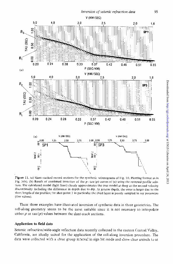
The combined inversion of the p-tau(p) curves using equation (5) results in the two velocity-depth functions beneath the shotpoints (Fig. 11). Both velocity models are in agreement with the input model for the depth to the second boundary. The dip of 4.6" can easily be calculated from the two depth estimates and the known separation between shotpoints. The velocity below the second boundary has not been correctly inverted due to the undersampling in p .

at USG

S Libraries on A


Dow

nloaded from


5.0

0.20

Inversion of seismic refraction data

V (KMISEC)

4;O 3,O 2.0

0.28 0.33 0.37 0.42 0.51 0.24 0.46

0.20 0.24

( b )

0.28

V (KMISEC)

P (SEC/KM)

V (KMISEC) 3.0 2.5

1 0.33 0.37 0.42

P ( S K ' K M )

1

0.46

V (KMISEC)

0.51

Figure 11. (a) Slant-stacked record sections for the synthetic seismograms of Fig. 10. Plotting format as in Fig. 5(b). (b) Result of combined inversion of the p-tau ( p ) curves of (a) using the reversed profile solution. The calculated model (light lines) closely approsimates the true model as deep as the second velocity discontinuity including the difference in depth due t o dip. At greater depth, the error is larger due to the short length o f t h e profiles; for shot point 1 in particular the third layer is poorly sampled in ray parameter (five values).

These three examples have illustrated inversion of synthetic data in three geometries. The roll-along geometry seems t o be the most suitable since it is not necessary to interpolate either p or tau ( p ) values between the slant-stack sections.

Application to field data

Seismic refraction/wide-angle reflection data recently collected in the eastern Central Valley, California, are ideally suited for the application of the roll-along inversion procedure. The data were collected with a close group interval in sign bit mode and show clear arrivals t o at

at USG

S Libraries on A


Dow

nloaded from


DIST

ANCE

(KM

)

Figu

re 1

1. S

eism

ic r

ecor

d se

ctio

ns re

cord

ed f

or t

he U

SGS

in t

he C

entr

al V

alle

y, C

alif

orni

a, i

n si

gn-b

it fo

rmat

with

23

m

grou

p in

terv

al.

Five

exp

losi

ve s

hots

hav

e be

en s

umm

ed t

o m

ake

each

rec

ord

sect

ion.

The

rol

l-alo

ng i

nver

sion

sol

utio

n (F

igs

6 an

d 7)

may

be

appl

ied

to t

his

data

. A

rrow

s in

dica

te t

he c

ross

-ove

r to

the

sei

smic

bas

emen

t w

ith a

n ap

pare

nt

velo

city

of 5

.8 k

m s-

!.

B a a s

at U

SGS

Lib

rari

es o

n A

pril

24, 2

013

http

://gj

i.oxf

ordj

ourn

als.

org/

Dow

nloa

ded

from


P

V (K

MIS

EC)

V (K

MIS

EC)

s L"

a 3

+

0.15

0.

19

0.23

0.

28

0.32

0.

37

0.41

0.

46

0.50

s L"

0.15

0.

19

0.23

0.

28

0.32

0.

37

0.41

0.

46

0.50

P (S

ECIK

M)

P (S

EC/K

M)

(b)

SP 8

70

V(KM

ISEC

) SP

928

V

(KM

ISEC

)

N

Figu

re 1

3. (

a) S

lant

-sta

cked

rec

ord

sect

ions

for

the

field

dat

a of

Fig

. 12

. Plo

tting

form

at a

s in

Fig

, 5(b

). (

b) R

esul

t of

com

bine

d in

vers

ion

of th

e p-

tau

(p)

curv

es o

f (a

) usi

ng t

he 'r

oll-a

long

' so

lutio

n. A

dif

fere

nce

of 1

50 m

in

the

dept

h to

sei

smic

bas

emen

t (v

eloc

ity g

reat

er t

han

6.0

km S-

')

has

been

res

olve

d.

;a" 3 E'

W

4

at U

SGS

Lib

rari

es o

n A

pril

24, 2

013

http

://gj

i.oxf

ordj

ourn

als.

org/

Dow

nloa

ded

from


98

least lOkm offset (Fig. 12). The sign-bit recording mode makes it possible to have a large number of channels (1024) but yields very low dynamic range (0-10 digital counts in this case). Seismic basement has a clear dip in this area; this is evidenced by the greater cross-over distance to the basement refractor for shot point (SP) 928 as compared to SP 870. The inversion procedure was applied to these data to resolve the lateral change in structure.

The record sections in Fig. 12 were slant stacked into the p-tau domain via equation (2) using a semblance threshold of 0.3 (Stoffa et al. 1981a) to obtain a better signal-to-noise ratio from this sign-bit data. The p-tau (p) curve has been automatically picked from the sections (Fig. 13a) using an initial (surface) velocity of 2.0 km s-'. The inverted velocity- depth curves (Fig. 13b) show a great similarity within the sedimentary section. The velocity contrast at the basement is from about 3.1 to 6.0 km s-', with the depth to basement below SP 928 about 150 m greater than below SP 870. This calculated difference is in good agreement with the difference in depth determined by drill-hole measurements (Bartow 1983). The velocity gradient in the basement is poorly resolved by a profile of this length.


Conclusions

The processing of seismic refractionlwide-aperture reflection data for laterally-varying velocity structures is an important aspect of data interpretation. We present a technique for processing densely spaced refraction data collected in three linear geometries (roll-along, split-spread, and reversed profiles), that is both automatic and stable for reasonable dips (up to about 8"). The technique consists of three steps: the slant stacking of the two time- distance wavefields to intercept-slowness wavefields, the picking of the p-tau (p) curve of principal arrivals using an L l-norm coherency measurement, and iterative downward stripping of the p-tau (p) curves. The resulting model consists of planar dipping isovelocity layers between shot points. The method has been successfully applied to all three types of geometries using synthetic data for a simple planar dipping structure. The most accurate results are for 'roll-along' geometry, and the application to real data have been illustrated.

The inversion scheme obtains, from the refracted and critically reflected arrivals, dip- corrected interval velocities which may be used as input data for the stacking of seismic reflection data. The results in all cases are compatible with those obtained from conventional processing, but the present method is significantly more objective and is particularly well suited to the automatic processing of large volumes of data. The present approach does not take into account the possible presence of low-velocity zones. The ease and practicality of the method encourage its further development and application.

Acknowledgments

Critical reviews by T. Brocher, M. Springer, P. A. Spudich, D. A. Stauber, G. A. McMechan and an anonymous reviewer are appreciated. We thank C. Wentworth and A. W. Walter for assistance in obtaining the sign-bit data tapes.

References

Bartow, J . A,, 1983. Map showing configuration of the basement surface, northern San Joaquin, Cali-

Brocher, T. M. & Phinney, R. A., 1981a. Inversion of slant stacks using finite-length record sections,

Brocher, T. M. & Phinney, R. A., 1981b. A ray parameter-intercept time spectral ratio method for seismic

fornia, USgeol. Surv. Misc. Field Studies Map MF-1430, scale 1 : 250,000.

J. geophys. Res., 86,7065-7012.

reflectivity analysis, J. geophys. Rex, 86,1865-1813.

at USG

S Libraries on A


Dow

nloaded from



Carrion, P. M. & Kou, J. T., 1984. A method for computation of velocity profiles by inversion of large

Carrion, P. M., Kuo, J. T. & Stoffa, P. L., 1984. Inversion method in the slant stack domain using ampli-

Eervenq, V., Moltokov, 1. A. & PSenElk, I . , 1977. Ray Method in Seismology, Charles University, Prague. Chapman, C. H., 1978. A new method for computing synthetic seismograms, Geophys. J. R. astr. Soc.,

Chapman, C. H . , 1981. Generalized radon transforms and slant stacks, Geophys. J. R. astr. SOC., 66,

Clayton, R. W. & McMechan, G. A., 1981. Inversion of refraction data by wave field continuation,

Claerbout, J. F., 1976. Fundamentals of Geophysical Data Processing, with Applications to Petroleum

Cunningham, A. S. , 1974. Refraction data from single ended refraction profiles, Geophysics, 39,

Diebold, J . B. & Stoffa, P. L., 1981. The traveltime equation, tau-p-mapping, and inversion of common

Durrani, T. S. & Bisset, D., 1984. The Radon transform and its properties, Geophysics, 49, 1180-1187. Fuis, G. S., Mooney, W. D., Healy, J. H., McMechan, G. A. & Lutter, W. J., 1984. A seismic refraction

studies of the Imperial Valley region, California, J. geophys. Res., 89, 1165-1189. Henry, M., Orcutt, J. A. & Parker, R. L., 1980. A new method for slant stacking refraction data,

Geophys. Res. Lett., 7, 1073-1076. Jannsen, D., Voss, J. & Theilen, F., 1985. Comparison of methods to determine Q in shallow marine

sediments from vertical reflection seismograms, Geophys. Prospect., in press. Johnson, S. H., 1976. Interpretation of split-spread refraction data in terms of plane dipping layers,

Geophysics, 41,418-424. Kennett, B. L. N., 1981. Slowness techniques in seismic interpretation, J. geophys. Res., 86, 1 1 575-

11 584. McMechan, G. A., 1983. p-x imaging by localized slant stacks of T-x data, Geophys. J. R. astr. SOC., 72,

213-221. McMechan, G. A., Clayton, R. W. & Mooney, W. D., 1982. Application of wavefield continuation to the

inversion of refraction data, J. geophys. Res., 87,927-935. McMechan, G . A. & Mooney, W. D., 1980. Asymptotic ray theory and synthetic seismograms for laterally

varying structures: theory and application to the Imperial Valley, California, Bull. seism. SOC. Am,

McMechan, C. A. & Ottolini, R., 1980. Direct observation of a p-tau curve in a slant stacked wavefield,

Muller, G., 1971. Direct inversion of seismic observations, Z. Geophys., 37, 225-235. Ocola, L. C., 1972. A nonlinear least-squares method for seismic refraction mapping - part 11: model

Phinney, R. A., Chowhury, K. R. & Frazer, L. N., 1981. Transformation and analysis of record sections,

Stoffa, P. L., Buhl, P., Diebold, J. B. & Wenzel, F., 1981a. Direct mapping of seismic data to the domain

Stoffa, P. L., Diebold, J. B. & Buhl, P., 1981b. Inversion of seismic data in the tau-p plane, Geophys.

Stoffa, P. L., Diebold, J. B. & BUN, P., 1982. Velocity analysis for wide aperture seismic data, Geophys.

Taner, M. T. & Koehler, F., 1969. Velocity spectradigital derivation and application of velocity functions,

Treitel, S., Gutowski, P. R. & Wagner, D. E., 1982. Plane wave decomposition of seismograms, Geophysics,

offset records, Geophysics, 49, 1249-1258.

tudes of reflection arrivals, Geophys. Prospect., 32, 375-391.

54,481-518.

445-453.

Geophysics, 46, 860-868.

Prospecting, McGraw-Hill, New York.

292-301.

midpoint data, Geophysics, 46,238-254.

70,2021-2035.

Bull. seism. SOC. Am., 70, 775-789.

studies and performance of REFRAMAP method, Geophysics, 37, 273-287.

J. geophys. Res., 86,359-377.

of intercept time and ray parameter - a plane wave decomposition, Geophysics, 46,255-267.

Res. Lett., 8,869-872.

Prospect., 3 0 , 2 5 4 7 .

Geophysics, 34, 859-881.

47,1375-1401.

Appendix: inversion of p-tau ( p ) curves for planar dipping structure

Two spatially dense seismic sets @ ( t , x ) ~ and @ ( t , x ) ~ are available from two shotpoints observed along a single profile line. Both data sets are slant stacked for the same number and range of ray parameters. Beginning with the starting surface velocity information p l = l / u l

at USG

S Libraries on A


Dow

nloaded from


100 and tau (pl) = 0, we automatically determine the curves of the principal arrivals [ p , tau ( p ) ] 1, from the slant stacked wavefields $(tau, p)l and $(tau, p ) 2 (see text). Both sets of discrete Lp, tau ( p ) l l , values are the input for an iterative inversion scheme to compute the layer thickness, velocity and dip.

Fig. A1 shows a model with n dipping layers and with the raypath. travel time and delay time geometry for rays critically reflected or bottoming at the nth boundary. Source or receiver positions are located at the surface at A, B, C, D and E. The intercept time tau (p,) for an apparent wave slowness p n can be expressed in terms of the layer thicknesses, z j , and the velocities, ui, below the shotpoint. Angles ai and bi against the vertical describe the raypath and angles yi describe the dip. We have,


and, at the bottoming point (last layer),

a n - 1 = a n - 1 Y n = bn - 1 + Y n

u, = u, - /sin 01, - 1 .

(A21

(A3 1 At the bottoming point of the critical reflection at the nth boundary, substituting b, - = n - 1 - 2y,, equation (Al) can be separated into two terms:

Term I describes the layer thickness z , - and the dip y , of the nth iayer while term I1 contributes the raypath from the surface to the IZ - 2 layer and back to the surface.

S P L I T - S P R E A D G E O M E T R Y

For split-spread geometry (shotpoint at position C and receivers at A and E; Fig. Al), all angles ai and bi for i = 1, 1.1 - 1 can be calculated using Snell's law recursively starting at the surface. At the receiver A a plane wave with the lower apparent slowness p n a A (updip) is

I g n ' " a " D I

I I I

Figure A l . Cross-section showing recorder and shot point locations (A, B, C, D and E) with geometry of ray paths and of the planar dipping-layer structure and of travel times for up- and downdip observations.

at USG

S Libraries on A


Dow

nloaded from


Inversion of seismic refraction data 101 (downdip) is observed and at receiver F a plane wave with the higher apparent slowness p,,

observed, and p, , A f p , , F. The intercept times at shotpoint C are equal:

tau (P,, A ) = tau @ I * , F ) . (A51

When the velocity at the surface u1 is known we obtain the take-off angles at the surface a l and b l with

a l = sin-' (ulp, , E ) , b l= sin-' ( u l p n , A ) . ('46)

The slant stacked data set for shotpoint C to A will contribute the updip angles b j and the data set C to E will contribute the downdip angles aj. We then solve equation (Al) or (A4) using both curves of principal arrivals [ p , tau(p)]l,2 to determine the unknown layer thickness z , - of the n-1 layer below shotpoint C and the velocity u, with dip y n of the nth layer. Below we present a processing flow chart for an n-layer model with two data sets [p , , tau ( p n ) l l . and a split-spread geometry (Fig. A2).

R E V E R S E D P R O F I L E S

For reversed profiles (shotpoints at A and D, separated by a distance X,) a plane wave from shotpoint A with an apparent downdip slowness p n , c will be observed at receiver C with the

Start with layer 2

Initialize the inversion

Takeoff angles at the surface

Raytracing through the uppermost n - z layers

(A41

Snell's law at

the ( 1 + 1 1 ' ~ interface

Next layer

Dip of the interlace (A21

Critical angle at the interface (A21

Velocity contrast (A31

Thickness 01 the (n - 1) laver (A41

sum = s u m t ( 2 , /v,)(cos(a,)+ coscb,)) I

I

Figure A2. Processing flow chart for an N-layer model with the two data sets [pl, , , tau(pl,,)] and [ p 2 , , , tau ( P ? , ~ ) ] obtained in a split-spread recording geometry.

at USG

S Libraries on A


Dow

nloaded from


102 delay time tau (pn c) . The reciprocal time (time along a given refractor from one shotpoint to the other, Fig. Al) will be


t r e c , A = tau ( P n , C ) +xlPn,C. ('47)

At receiver B a plane wave from shotpoint D bottoming at the same boundary is observed

The reciprocal time will be with an apparent updip slowness pn , B and the delay time tau (pn, B).

trec, D = tau (Pn. B) + xl Pn, B = tau b n , C) + xl Pn, C = t r e c , A (A81

Pn, C # P n , B and tau (Pn, C) # tau (pn, B). (-49)

al = sin-' ( u l p n , c),

but neither the apparent slownesses nor the associated delay times are the same:

Again, we obtain the angles ai and bi recursively for i = 1, n - 1 starting at the surface with:

bl = sin-' ( u l p n , B). (A10)

The data set A to C will contribute the downdip angles ai and the data set D to B will contribute the updip angles bi we need to solve equation (Al) or (A4) for the unknown layer thicknesses z , - of the n-1 layer beneath shotpoints A and D and the velocity u, with dip yn of the nth layer.

R O L L-ALON G P R 0 FILES

For the roll-along technique (shotpoints at positions A and B, separated by a distance X2) a plane wave from shotpoint A with an apparent slowness pn,c will be observed at receiver C with the delay time tau ( p n , c ) (Fig. Al). At receiver D a plane wave from the same interface from Sjlotpoint B is observed with an apparent slowness pn , and the delay time tau (pn, D). The observed apparent slowness p n is not directly related to the layer velocity u, :

P n , C = P n , D f I / U n , n'l. (A1 1)

Planar dipping structure requires different delay times for the same apparent slownesses p n from the two shotpoints:

tau (Pn, C) # tau (Pn, D).

Rewriting equation (A4) for shotpoints A and B:

tau (pn, c ) = n - 1 Z 2 (cos ai + cos bi)

i = l ui.

(A141 B , i n - 1 z

tau (pn, D) =

where zA, i and zB , i are the thicknesses af the ith layer below shotpoints A or B respectively. The data sets A to C and B to D will only contribute the downdip angles ai. Starting at

the surface with

- (COS ai + cos bi) j = l U i

..

al = sin-' ( u l p n , c) = sin-' ( u l p , , D) (A15)

at USG

S Libraries on A


Dow

nloaded from



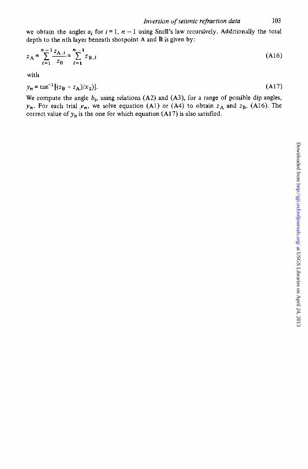
we obtain the angles ai for i = 1, n - 1 using Snell's law recursively. Additionally the total depth to the nth layer beneath shotpoint A and B is given by:

with

yn = tan-' [ ( Z B - zA)/xZ>l. (A1 7) We compute the angle bi, using relations (A2) and (A3), for a range of possible dip angles, y,. For each trial y , , we solve equation ( A l ) or (A4) to obtain Z A and ZB, (A16). The correct value of y, is the one for which equation (A17) is also satisfied.

at USG

S Libraries on A


Dow

nloaded from


accepted 1984 december 26. received 1984 … · inversion of seismic refraction data 83 gutowski...

Documents