HAL Id: hal-01553004https://hal.archives-ouvertes.fr/hal-01553004

Submitted on 3 Jul 2017

HAL is a multi-disciplinary open accessarchive for the deposit and dissemination of sci-entific research documents, whether they are pub-lished or not. The documents may come fromteaching and research institutions in France orabroad, or from public or private research centers.

L’archive ouverte pluridisciplinaire HAL, estdestinée au dépôt et à la diffusion de documentsscientifiques de niveau recherche, publiés ou non,émanant des établissements d’enseignement et derecherche français ou étrangers, des laboratoirespublics ou privés.

Accounting for Acoustic Damping in a Helmholtz SolverFranchine Ni, Maxence Miguel-Brebion, Franck Nicoud, Thierry Poinsot

To cite this version:Franchine Ni, Maxence Miguel-Brebion, Franck Nicoud, Thierry Poinsot. Accounting for AcousticDamping in a Helmholtz Solver. AIAA Journal, American Institute of Aeronautics and Astronautics,2017, 55 (4), pp.1205-1220. �10.2514/1.J055248�. �hal-01553004�

Open Archive TOULOUSE Archive Ouverte (OATAO) OATAO is an open access repository that collects the work of Toulouse researchers andmakes it freely available over the web where possible.

This is an author-deposited version published in : http://oatao.univ-toulouse.fr/Eprints ID : 17947

To link to this article : DOI:10.2514/1.J055248URL : http://dx.doi.org/10.2514/1.J055248

To cite this version : Ni, Franchine and Miguel-Brebion, Maxenceand Nicoud, Franck and Poinsot, Thierry Accounting for AcousticDamping in a Helmholtz Solver. (2017) AIAA Journal, vol. 55 (n° 4).pp. 1205-1220. ISSN 0001-1452

Any correspondence concerning this service should be sent to the repository

administrator: staff-oatao@listes-diff.inp-toulouse.fr

Accounting for Acoustic Damping in a Helmholtz Solver

F. Ni∗

Centre Européen de Recherche et de Formation Avancée en Calcul Scientifique,

31057 Toulouse, France

M. Miguel-Brebion†

Institut de Mécanique des Fluides de Toulouse, 31400 Toulouse, France

F. Nicoud‡

Université de Montpellier, 34095 Montpellier, France

andT. Poinsot§

Institut de Mécanique des Fluides de Toulouse, 31400 Toulouse, France

DOI: 10.2514/1.J055248

Thermoacoustic Helmholtz solvers provide a cheap and efficient way of predicting combustion instabilities.

However, because they rely on the inviscid Euler equations at zeroMach number, they cannot properly describe the

regions where aerodynamics may interact with acoustic waves, in the vicinity of dilution holes and injectors, for

example. A methodology is presented to incorporate the effect of non-purely acoustic mechanisms into a three-

dimensional thermoacoustic Helmholtz solver. The zones where these mechanisms are important are modeled as

two-port acoustic elements, and the corresponding matrices, which notably contain the dissipative effects due to

acoustic–hydrodynamic interactions, are used as internal boundary conditions in theHelmholtz solver.The rest of the

flow domain, where dissipation is negligible, is solved by the classical Helmholtz equation. With this method, the

changes in eigenfrequency and eigenmode structure introduced by the acoustic–hydrodynamic effects are captured,

while keeping the simplicity and efficiency of the Helmholtz solver. The methodology is successfully applied on an

academic configuration, first with a simple diaphragm, then with an industrial swirler, withmatrices measured from

experiments and large-eddy simulation.

I. Introduction

C OMBUSTION instabilities are a major issue for moderncombustion engines, such as rockets, turbojet engines, or gas

turbines [1–3].When the fluctuations of pressure and heat release arein phase, a coupling between flame and acoustics creates strongpressure oscillations in the combustor, potentially leading to animportant structural damage or even a catastrophic engine failure.From an academic perspective, the phenomenon has been studiedsince the 1900s [4], but is still not fully understood. It is, therefore, anintense topic of research among the combustion community [5,6].For engine manufacturers, combustion instabilities must be

avoided, preferably early enough in the design stage. There isconsequently a need for numerical tools capable of predicting thestability of a combustor even before it is built. These tools range fromsimple network models that are fast and easy to implement [7–11]tomore complex and time-consuming large-eddy-simulation (LES)solvers [12–18]. In-between, linearized Navier–Stokes equation(LNSE) solvers and Helmholtz solvers provide a fair tradeoffbetween computational cost and fidelity. They are suitable forcomplex three-dimensional (3-D) industrial geometries, but aresimpler and faster than LES. LNSEs have the merit of directlyincluding acoustic–hydrodynamic effects as demonstrated forsimple two-dimensional (2-D) and 3-D configurations [19–21], butto the authors’ knowledge, most LNSE studies focus on the

propagation of acoustic fluctuations in nonreactive flows. In thecontext of combustion instabilities, we are more interested indetermining the eigenmodes of a reactive flow, and this is wellachieved by a Helmholtz solver. Compared to LNSE solvers,Helmholtz codes solve the linearized inviscid Euler equations witha baseline flow at rest, and require less computational power andless refined meshes. This simplicity comes at a price, because anymechanism implying interactions with fluid viscosity, heat transfer,or hydrodynamics is left apart. In a typical combustor (Fig. 1), evenif the zero Mach-number assumption is justified in most of thedomain, these mechanisms could still have an acoustic impact(Table 1) [22–36].Some of these contributions are well known and can be accounted

for in the Helmholtz solution. This is the case of the acoustic lossescreated at thermoviscous boundary layers. When acoustic wavesinteract with the boundary layers, acoustic energy is dissipatedthrough shear stress and heat losses. A synthetic model has beenproposed by Searby et al. [25] and is of great interest because it can beused to postprocess a Helmholtz computation. The treatment extractsthe damping rate due to thermoviscous effects for any standing modecomputed by the dissipation-free Helmholtz solver.One interesting observation in the study of Searby et al. [25] is

that thermoviscous damping scales as the square root of the frequency,and is therefore a high-frequency phenomenon, more common inrocket engines than in turbojet engines. Most of the unstable modesencountered in turbine combustion chambers have low-enoughfrequencies to neglect thermoviscous damping. At these frequencies,another mechanism is at stake. When a mean flow is present, a shearlayer is created at sudden section changes and can extract energy fromthe acoustics by converting it intovorticity [28,31,37,38]. In the case ofperforated plates, such as the ones involved in cooling the combustorwalls (see Fig. 1), the impact on acoustics can be quantified using, forexample, Howe’s model [28], as recalled in Appendix A.Howe’s model and its counterparts [29,30,39] can be used to

represent perforated plates as homogeneous boundary conditions in aHelmholtz solver [32] or in a computational fluid dynamics (CFD)code [30]. For more complex systems, such as swirlers, no analyticalmodel is available to describe the acoustic–hydrodynamic effects.

Still, provided that such a complex system behaves like a linear time-invariant causal system, it can be abstracted as a 2 × 2 matrix in thefrequency domain. The latter can be measured experimentally[40,41] or numerically [42]. Themethod is well known, and has oftenbeen used in the acoustic analysis of ducts and mufflers [35,43–45],and flame dynamics [46–48]. Some studies also report results onswirlers [34] and heat exchangers [49]. The equivalent matrix can beplugged into an acoustic network to provide results for complexconfigurations by decomposing them into simpler elements[43,50,51].In this paper, we propose to incorporate this matrix formalism into a

Helmholtz solver, in a similarway towhatwasproposedbyCampaandCamporeale [52] and Laera et al. [53].With this approach, the acousticimpact of non-purely acoustic mechanisms can be reproduced in theHelmholtz solver for very general systems (for example, the swirlerand the dilution holes in Fig. 1), so that the result ismore representativeof an actual combustor. Whereas the work of Laera et al. [53] uses thematrix formalism mainly to describe flame–acoustics coupling, thepresent work deals with the dissipative effects due to acoustic–hydrodynamic interaction. Themethodology is applied to an academicconfiguration containing a dissipative element (first a diaphragm, thena swirler), whose dissipative behavior is quantified experimentally andby the proposed enhanced Helmholtz-solver approach. The targetconfiguration is also computedwith LES so that comparisons betweenthe Helmholtz solver, the LES computation, and experimental resultscan be provided.The paper is structured as follows. The methodology and its

practical implementation in a Helmholtz solver are presented inSec. II. To check its validity, comparisons between LES,experiments, and Helmholtz-solver results are performed for anacademic configuration. The overall validation strategy and the targetconfiguration are described in Sec. III. The results are then presentedfor a diaphragm in Sec. IV, and for an industrial swirler in Sec. V.

II. Description of the Methodology

As briefly stated in the Introduction, we propose to model thedissipative behavior of an element inside an inviscid domain by

measuring its two-port matrix. The concept is well definedwhen planemodes are considered. The acoustic states up- and downstream of thedissipative zone are fully described by two quantities, for example, p 0and ρocou 0, the acoustic pressure and velocity fluctuations, orA� ��p 0 � ρo � co � u 0�∕2 and A− � �p 0 − ρo � co � u 0�∕2 the rightand left traveling waves. The direction of the longitudinal axis x ischosen so that u 0 > 0 corresponds to a velocity perturbation movingtoward the right. For a linear system, the upstream and downstreamstates are connectedbya2 × 2matrix; seeFig. 2.WhenA� andA− areused instead, this matrix is called the scattering matrix. Otherconventions exist, and some are listed in Table 2.In the following, we show how the damping effect of acoustic–

hydrodynamic systems can be included in a typical 3-Dthermoacoustics Helmholtz solver (the AVSP solver [54] in thisstudy). For this purpose, the zones that cannot be described byacoustics only are removed from the domain where the Helmholtzequation is solved, and replaced by their 2 × 2 matrix (Fig. 3). Thisoperation requires the coupling of a 3-DHelmholtz solver with a two-port matrix, which is achieved by a matrix boundary condition(MBC) described next. Dissipative effects located at the boundariesof the total fluid domain, such as radiation, aremodeledwith classicalimpedances (Fig. 3).The acoustic quantities are decomposed asp 0�x; t� � R�p�x�e−iωt�

and u 0�x; t� � R�u�x�e−iωt�, assuming a harmonic time dependenceand a spatially varying amplitude. Their behavior in the frequencydomain is determined by the Helmholtz equation (1) (given here in theabsence of a source term) and the linearized momentum equation (2).

Table 1 Examples of non-purely acoustic mechanisms presentin a typical combustor (Fig. 1)

Mechanism Location in combustorAvailablemodels

Acoustic losses in thermal andviscous boundary layers

No-slip walls,nonadiabatic walls

[22–25]

Drag/thermal losses due to liquidparticles

Liquid spray [26,27]

Acoustic–hydrodynamic interactionsat perforated plate

Multiperforated plates [28–33]

Acoustic–hydrodynamic interactionsat other elements

Swirler, dilution holes,T-junctions

[21,34–36]

Fuel supply1

Air supply2

Swirler3

Liquid fuel spray4

Flame5

Multiperforated plate6

Dilution hole7

1

2

3

4

4 5

6

6

7

7

To turbine

To compressor

Fig. 1 Typical turbojet combustor design and its components.

Fig. 2 Modelization of an acoustic system (here, a slit) as a two-portfilter.

Table 2 Examples of acoustic two-port formulation (from [34])

Name State variables Defining equation

Transfer matrix p 0, u 0�p 0d∕�ρo;dco;d�

u 0d

�≡ Ta

�p 0u∕�ρo;uco;u�

u 0u

�

Scattering matrix A�, A−�A�

d

A−u

�≡ S

�A�

u

A−d

�

Mobility matrix p 0, u 0�u 0u

u 0d

�≡M

�p 0u∕�ρo;uco;u�

p 0d∕�ρo;dco;d�

�

γPo�x�∇ ·

�1

ρo�x�∇p�x�

�� ω2p�x� � 0 (1)

u � 1

ρoiω∇p (2)

with γ the ratio of specific heats (constant, equal to 1.4 for ambient air)and Po the temporal average of the pressure. The Helmholtzeigenvalue problemmade up of Eqs. (1) and (2) is discretized at nodesand solved by the AVSP solver [54] with a finite volume strategy. Toclose the problem at boundaries, information about the pressuregradient along the boundary normal must be provided in the form ofpressure boundary conditions (Fig. 4). To account for the two-portmatrix in the truncated flow domain, a new boundary condition shouldtherefore be defined, which relates the pressure fluctuation p to itsgradient. This is obtained by combining the mobility-matrixformulation (last row of Table 2) with the linearized momentumequation (2).

8<:∇pu · nu � M11

iωco;u

pu �M12iωco;d

ρo;uρo;d

pd

∇pd · nd � M22iωco;d

pd �M21iωco;u

ρo;dρo;u

pu

(3)

in which the upstream and downstream boundary normal vectors nu

andnd are defined with an inward normal convention (Fig. 3). System(3) defines a pair of Robin conditions suited to represent the effect of anon-purely acoustic element, including its dissipation (Fig. 3). Theseboundary conditions are applied pointwise to a pair of patches. To linkthe noncoincident upstream and downstream meshes, the nodes ofeach patch are projected onto the other, and the field of p is linearlyinterpolated on the projected nodes.With theMBC, it is possible to account for nonacoustic elements in

a Helmholtz solver with the following strategy:1) Remove all dissipative/nonacoustic zones from the domain.

Note that this is different from the LNSE approach, in which thedissipative elements need to be meshed. Once the dissipationmatrices are obtained, the MBC procedure runs with lighter andsimpler meshes than the LNSE ones.

2) Link the remaining inviscid domains with a pair of internalMBCs, representative of the element previously removed.3) Solve the discretized Helmholtz eigenproblem with the MBC

internal boundaries. Note that the introduction of MBC makes theHelmholtz eigenproblem nonlinear with respect to the eigenvalues,because the eigenproblem operator at boundaries nowdepends on theeigenfrequency; see Eq. (3). The problem remains, however, linearwith respect to the eigenvectors (pressure mode shape), because nodependency with the amplitude is considered in this study. Thenonlinear eigenvalue search is treated in AVSP with a fixed-pointloop described in [54].As a verification test, it was checked (not shown) that the MBC

implementation matches the analytical eigenmodes and eigenfre-quencies in cases inwhich analytical solutions are available [e.g., 2-Dtubes connected by a simple identity matrix or the matrixcorresponding to Howe’s model, Eq. (A1)].

III. Validation Strategy

In the configuration described in Fig. 3, the conventionalHelmholtz solver cannot account for the dissipative effects created byacoustic–hydrodynamic interactions at the swirler even if the wholegeometry of the latter is represented by the finite volume mesh.However, adding the MBC should improve the results. To apply theMBC methodology, the matrix of the dissipative element is requiredand must be retrieved either experimentally or numerically. To checkwhether the resulting eigenfrequencies and eigenmodes are “better”than without MBC, they are compared to reference eigenmodes andeigenfrequencies, which are again either computed by LES ormeasured in experiments.This section explains how the MBC methodology is applied to a

target configuration described in Sec. III.A. For this configuration,the matrix data and reference eigenpairs are obtained fromexperiments (Sec. III.B) and from LES (Sec. III.C). The matrices areused to define MBC in the Helmholtz computation of the truncateddomain. The corresponding numerical setup is presented inSec. III.D.To check the validity of the MBC methodology, four types of

comparisons, called C1, C2-LES, C2-EXP, and C3 in Fig. 5, areperformed:1) C1: Matrices obtained from the experiments and from the LES

are compared, to check their validity and robustness to eithernumerical or experimental artifacts.2) C2-LES: The LES-matrix data are used as an input of the

Helmholtz solver with MBC. The resulting eigenfrequencies andeigenmodes are compared with the LES values, and with the resultsof the Helmholtz solver without MBC.3) C2-EXP: The experimental-matrix data are used as an input of

the Helmholtz solver with MBC. The resulting eigenfrequencies andeigenmodes are compared with the experimental values and with theresults of the Helmholtz solver without MBC.

Invisciddomain 1 Invisciddomain 2

Matrix BoundaryCondition

Dissipative zone

Radiation losses

Helmholtz domain 1 Helmholtz domain 2 Radiation Impedance

Actualconfiguration

Truncatedconfiguration with MBC

Temporal domain

Frequencydomain

nu nd

Fig. 3 Locally dissipative elements inside a globally inviscid domain are modeled by two-port matrices.

Fig. 4 Discretization of a 2-Dboundarynode inAVSP (dual cell in grey).

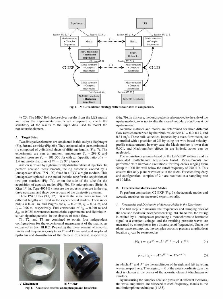
4) C3: The MBC Helmholtz-solver results from the LES matrixand from the experimental matrix are compared to check thesensitivity of the results to the input data used to model thenonacoustic element.

A. Target Setup

Two dissipative elements are considered in this study: a diaphragm(Fig. 6a) and a swirler (Fig. 6b). They are installed in an experimentalrig composed of cylindrical ducts of different lengths (Fig. 7). Theexperiments are run at ambient temperature To � 299 K andambient pressure Po � 101; 550 Pa with air (specific ratio of γ �1.4 and molecular mass of W � 28.97 g∕mol).Airflow is driven by eight uniformly distributed radial injectors. To

perform acoustic measurements, the rig airflow is excited by aloudspeaker (Focal ISN 100) fixed in a PVC airtight module. Thisloudspeaker is placed at the end of the inlet tube for the acquisition oftwo-port matrices (Fig. 7a), or on the side of the tube for theacquisition of acoustic modes (Fig. 7b). Six microphones (Brüel &Kjær 1/4 in. Type 4954-B) measure the acoustic pressure in the rig:three upstream and three downstream of the dissipative element.Three PVC tubes (T1, T2, T3) with the same cross section but

different lengths are used in the experimental studies. Their innerradius is 0.041 m, and lengths are l1 � 0.26 m, l2 � 0.34 m, andl3 � 0.56 m, respectively. End corrections of δin � 0.010 m andδout � 0.025 mwere used tomatch the experimental andHelmholtz-solver eigenfrequencies, in the absence of mean flow.T1, T2, and T3 are combined to obtain four independent

configurations for the experimental measurement of the matrix, asexplained in Sec. III.B.2. Regarding the measurement of acousticmodes and frequencies, only tubes T3 andT2 are used, and are placedupstream and downstream of the element of interest, respectively

(Fig. 7b). In this case, the loudspeaker is also moved to the side of theupstream duct, so as not to alter the closed boundary condition at theupstream end.Acoustic matrices and modes are determined for three different

flow rates characterized by their bulk velocities: U � 0.0, 0.17, and0.34 m∕s. These bulk velocities, imposed by a mass-flow meter, arecontrolled with a precision of 2% by using hot-wire-based velocity-profile measurements. In every case, the Mach number is lower than0.001, and Mach-number effects in the inviscid zones can beneglected.The acquisition system is based on the LabVIEW software and its

associated multichannel acquisition board. Measurements areperformed with harmonic excitations, for frequencies ranging from50 up to 1000 Hz, well below the cutoff frequency of 2500 Hz. Thisensures that only plane waves exist in the ducts. For each frequencyand configuration, samples of 2 s are recorded at a sampling rateof 10 kHz.

B. Experimental Matrices and Modes

To perform comparison C2-EXP (Fig. 5), the acoustic modes andacoustic matrices are measured experimentally.

1. Frequencies and Dissipation of Acoustic Modes in the Experiment

The first step is to measure the frequencies and damping rates ofthe acoustic modes in the experiment (Fig. 7b). To do this, the test rigis excited by a loudspeaker producing a monochromatic harmonicsignal at a constant voltage, and the resulting pressure waves aremeasured bymicrophones for a discrete set of frequencies. Under theplane-wave assumption, the complex acoustic-pressure amplitude atlocation zj can be expressed as

p�zj� � ajeiϕj � A�eik�zj �A−e−ik

−zj (4)

ρocou�zj� � A�eik�zj −A−e−ik−zj (5)

in whichA� andA− are the amplitudes of the right and left travelingwaves, respectively. The origin z � 0 of the axial coordinate zj in theduct is chosen at the center of the acoustic element (diaphragm orswirler).Bymeasuring the complex acoustic pressure at different locations,

the wave amplitudes are retrieved at each frequency, thanks to themultimicrophone technique [41,55].

Experiments LES

MBC-Helmholtz + Radiation impedance

Matrix Matrix Mode structure

+ Complex frequencies

Mode structure + Complex frequencies

Mode structure + Complex frequencies

C1

MBC-Helmholtz

Mode structure + Complex frequencies

C2-EXP C2-LES

NoMBC-Helmholtz + Radiation impedance

Mode structure + Complex frequencies

NoMBC-Helmholtz

Mode structure + Complex frequencies

C3

Section III. B. 1. Section III. B. 2. Section III. C. 1. Section III. C. 2.

Section III. D.

Section III. D.

Section III. D.

Section III. D.

Fig. 5 MBC validation strategy with its four axes of comparison.

Fig. 6 Acoustic elements: a) diaphragm and b) swirler.

0@ eik

�z1 e−ik−z1

: : : : : :eik

�zJ e−ik−zJ

1A

|��������������{z��������������}D

�A�

A−

�|��{z��}

x

�0@ a1e

iϕ1

: : :aJe

iϕJ

1A

|�����{z�����}b

(6)

~x � �D†D�−1D†b (7)

System (6) is overdetermined when more than two microphonesare used, and is inverted with a least-squares approach as donein Eq. (7).The wave amplitudes are combined to reconstruct E, the period-

averaged acoustic energy integrated over the volume V of the rig, asdefined in Eq. (8).

E �ZV

�1

4ρoc2o

jp�z�j2 � 1

4ρoju�z�j2

�dV (8)

For planewaves at lowMach number in a forced harmonic regime,the wave amplitudes are constant in each inviscid rig portion, and theterm in the integral of Eq. (8) is independent of the coordinate z. Theintegration can thus be performed separately over the upstream and

downstream volumes Vu and Vd to obtain Eq. (9).

E�ω� � Vu

�1

2ρoc2o

hjA�

u �ω�j2 � jA−u �ω�j2

i�

� Vd

�1

2ρoc2o

hjA�

d �ω�j2 � jA−d �ω�j2

i�(9)

The spectrum of acoustic energy E�ω� contains information aboutthe eigenfrequencies of the system, in the form of resonance peaks(Fig. 8). A fit is performed on these peaks to retrieve the complexeigenfrequencies [56,57] based on the idea that the complex waveamplitudes A� and A− in the system are solutions of a dampedoscillator equation of the form:

�η�t� − 2ω0i _η�t� � ω20rη�t� � F (10)

in which F � Fe−iωt is the harmonic-forcing term, and η�t� isto be replaced byA�e−iωt orA−e−iωt. The forcing angular frequencyω is to be distinguished from the unknown complex angulareigenfrequencyω0 � 2πf0 � ω0r � iω0i, whose imaginary partω0i

is the growth rate. Equation (10) is valid only for negative values ofω0i, corresponding to purely damped acoustics, as is the case here.

520 540 560 580 600 620 640 660 680 700f (Hz)

0.0

0.2

0.4

0.6

0.8

1.0

f(N

orm

aliz

ed)

Experimentaldata

Model

a) Mode 4 at (603.5 ± 0.1) -i(2.9 ± 0.1) Hz

680 700 720 740 760 780 800 820f (Hz)

0.0

0.2

0.4

0.6

0.8

1.0

1.2

1.4

f(N

orm

aliz

ed)

Experimentaldata

Model

b) Mode 5 at (748.9 ± 3.5) -i(13.4 ± 5.0) Hz

Fig. 8 E�ω� spectra for two modes of the diaphragm case at U � 0.17 m∕s.

a) Matrix measurement. The downstream part can be modified as shown in Fig. 9

b) Acoustic mode measurement

Loudspeaker

Lou

dspe

aker

Fig. 7 Sketch of the experimental setup for a) matrices and b) acoustic modes measurement.

Transposing Eq. (10) in the Fourier domain gives an expression forA� and A− as a function of ω0r and ω0i, which is combined withEq. (9) to yield an expression for E�ω�:

Etheo�ω� �1

2π

G

�ω20r − ω2�2 � 4ω2

0iω2

(11)

with G � jFj2�Vup � Vdown�∕�2ρoc2o�. This is the form used to fitE�ω�. The three parametersG,ω0r, andω0i are tuned so that Eq. (11)produces the best possible match of the measured spectrum E�ω�.This method is equivalent to but more precise than measuring thewidth at half-height of the peaks [57,58]. The quality of the fit isassessed by computing the uncertainty on f0 � �ω0r � iω0i�∕�2π�with a 95% confidence interval. This uncertainty displayed as a value in the captions of Fig. 8 is low when the data are well fitted(Fig. 8a), and increases as soon as the quality of the fit deteriorates,when the signal is noisy, for example (Fig. 8b). In Fig. 8, E�ω� isnormalized by the value fitted at ω0.

Once the eigenfrequencies are estimated, the associatedeigenmodes and acoustic fields can easily be reconstructed usingEqs. (4) and (5).

2. Experimental Two-Port Matrices

The two-port matrix is reconstructed following [59], with thescattering-matrix formalism (see Table 2). This requires at leasttwo linearly independent configurations. More robust results areobtained by using four independent configurations. In this study,this is achieved by combining in different ways the three ducts T1,T2, and T3, and switching the outlet impedance from open to closed(Fig. 9). For each configuration, the wave amplitudes are measuredupstream and downstream of the acoustic element of interest withthe multimicrophone technique exposed previously. As in themultimicrophone technique, an overdetermined system (12) isdefined from the four independent configurations of Fig. 9 with the

matrix coefficients S ��tu rdru td

�as unknowns, and inverted with

a least-squares approach.

0BBBBBBBBBBBBBB@

A�u;1 A−

d;1 0 0

0 0 A�u;1 A−

d;1

..

. ... ..

. ...

A�u;j A−

d;j 0 0

0 0 A�u;j A−

d;j

..

. ... ..

. ...

A�u;N A−

d;N 0 0

0 0 A�u;N A−

d;N

1CCCCCCCCCCCCCCA

|��������������������������{z��������������������������}H

0BB@turdrutd

1CCA

|�{z�}s

�

0BBBBBBBBBBBBBB@

A�d;1

A−u;1

..

.

A�d;j

A−u;j

..

.

A�d;N

A−u;N

1CCCCCCCCCCCCCCA

|����{z����}a

(12)

~s � �H†H�−1H†a; errrelative � kH ~s − ak∕kak (13)

Equation (13) provides the scattering-matrix coefficients, as wellas an estimation of the least-squares error. The second index j runsfrom 1 to N � 4, and denotes the ith independent state. This

scatteringmatrix is easily converted into themobility matrix requiredfor the MBC.

C. LES Matrices and Modes

The two-port matrices and acoustic eigenmodes can also bedetermined through LES computations performed with the AVBPsolver, codeveloped by the Centre Européen de Recherche et deFormation Avancée en Calcul Scientifique (CERFACS) and the InstitutFrançais du Pétrole Energies Nouvelles (IFPEN) [60]. This solver iswidely used and has been validated in numerous situations[15,18,30,61–64], to cite a few. The results will serve to check theexperiments in comparison C1 and to perform comparison C2-LES(Fig. 5). The numerical parameters and boundary conditions based onthemodels in [65–68] aregiven inAppendixB.This section presents themethodology used to obtain the numerical matrices and eigenmodes.

1. LES Matrices

To compute the two-port matrix from the LES data, twoindependent harmonic-forcing states are used [59,69]. In state 1, theacoustic element is excited from the inlet, with a nonreflectivecondition prescribed at the outlet. In state 2, the acoustic element isexcited from the outlet, with a nonreflective inlet. This is the onlydifference with the approach used in the experiments, in which theindependent states were obtained by changing the outlet impedance,while always forcing at the inlet.The geometry and overview of the mesh are shown in Fig. 10 for

the diaphragm, and Fig. 11 for the swirler. The duct lengths used inthe LES do not have to correspond to the experimental tubes. Theywere chosen long enough to let acoustic waves become one-dimensional away from the dissipative elements, and short enough tominimize computational times. The swirler vanes are discretizedwith18 points along the smallest dimension, and the diaphragm ismeshedwith 40 points in the diameter. Both meshes contain a few millionnodes (2.5 million points for the swirler and 1 million points for thediaphragm).The pressure is measured at probes equidistributed along the

pipe circumference for several axial locations. For the diaphragm,7 upstream stations and 11 downstream stations are used. For theswirler, only four upstream stations and five downstream stations areused because the hydrodynamic fluctuations created by the swirlerextend further than in the diaphragm case. The wave amplitudes andthe scattering matrix are then reconstructed with the same method asfor the experimental data.

2. LES Eigenmodes and Damping Rates

The experimental data provide references for the realeigenfrequencies and the associated mode structure. This wasobtained by forcing the experiment at hundreds of frequencies and

Fig. 10 LES geometry and mesh overview for the pulsed computationsof the diaphragm.Fig. 9 Configurations used to measure the matrices in the experiments.

constructing the E�f� curve of Fig. 8, which is not practical in LES.Therefore, a different method is used to obtain the dissipation ratesfrom LES: the acoustic-mode-triggering (AMT) approach [70].The idea of the AMT is to superimpose a given acoustic mode

(computed from a Helmholtz solver, say) to the mean flowfieldscomputed by a nondisturbed LES [70]. The resulting disturbedsolution is used to initialize a new LES computation, in which theinitial acoustic perturbations are damped by the presence of thediaphragm or swirler. No forcing is applied. The acoustic system issimply initially displaced from equilibrium. As for a dampedoscillator, this results in decaying acoustic oscillations, whose decayrate and frequency are captured by the LES (Fig. 12).

The geometries used in the AMT computations are basically thesame as those used for the pulsed computations (Figs. 10 and 11),but the duct lengths are modified to match the experimental ductlengths, plus the end corrections. The mesh refinement is the sameas for the pulsed computations. Avelocity-imposed, fully reflectiveboundary condition is enforced at the inlet. For the outlet, apressure-imposed characteristic condition with relaxation toward atarget value was tuned to obtain a reflection coefficient withradiation losses [71] Rrad�ω� � −�1∕4�ka�2 − 1�∕�1∕4�ka�2 � 1�(with a the pipe radius). The formulation of the outlet boundarycondition is an extension of the one described in the work of Selleet al. [61]. With their notation, the incoming wave amplitude L1 isset to L1 � K�P − P∞� − RKL5, and the associated reflectioncoefficient is (Fig. 13)

RLES�ω� � −RK −1 − RK

1 − �2iω∕K� (14)

with K the relaxation coefficient and RK the value of the reflectioncoefficient when K → 0. A cut-off frequency can be defined asfc � K∕4π, at which the phase is equal to π � ϕ withϕ � tan−1��1 − RK�∕�1� RK��. For the diaphragm, K is fixed toensure no pressure drift, whereasRK is adjusted to set jRLESj�ω0� �jRrad�ω0�j at the desired angular frequency ω0 (Table 3). For theswirler, K is fixed to the highest value allowed in the LES code toobtain a fully reflective boundary, as will be recalled later.To measure the real frequency and damping rate, the dynamic

mode decomposition (DMD) [72] is performed on the pressure andvelocity signals measured at upstream and downstream probes. TheDMD is able to isolate the frequency of the excited mode and itsdecay rate. Figure 12 shows an example of such a filtering for a probe

0 5 10 15 20 25 30Time [ms]

102560

102580

102600

102620

102640

102660

102680

102700

Pres

sure

[Pa]

exp 2π fi t

0 5 10 15 20 25 30Time [ms]

0.20

0.25

0.30

0.35

0.40

0.45

0.50

Vel

ocity

[m/s

]

exp 2π fi t

LES

DMD - reconstruction at f = 284.9-13.2j Hz

Fig. 12 DMD reconstruction of the pressure (left) and velocity (right) signal at a probe.

Fig. 11 LESandmeshoverview for thepulsedcomputationsof the swirler.

0 fc 10 fc

RK

1

RL

ES

0 fc 10 fc

π

π φ

arg

RL

ES

Fig. 13 Modulus (left) and phase (right) of the AMT outlet reflectioncoefficient RLES.

signal in the AMT computation of the swirler (U � 0.34 m∕s andf � �284.9–13.2i� Hz). DMD also provides the amplitude andphase of the acoustic fluctuations for each frequency. Thisinformation could be used directly to reconstruct the eigenmode, butan additional least-squares fit was performed to determine theacoustic quantities as a sumof plane-wave amplitudes, as done for theexperiments in Sec. III.B.1. The pressure signals at LES probes areused to construct system (6) that is inverted using Eq. (7). Thisprocedure smoothes the acoustic fields and helps separate them fromnoise or hydrodynamic fluctuations (Fig. 14).

D. Helmholtz-Solver Eigenmodes and Eigenfrequencies with MBCBoundaries

Once the experimental (Sec. III.B.2) and LES (Sec. III.C.1)matrices are measured, they can be used in the Helmholtz solver withMBC. To use the MBC, the setup geometry has to be modified. Asexplained in Sec. II, the acoustic element is not meshed anymore.Instead, the upstream and downstream tubes are cut so as to removecompletely the acoustic element. The matrices constructed inSecs. III.B.2 and III.C.1 are used to represent adequately thetransition between up- and downstream cuts (Fig. 15b).At the test-rig ends, the boundary conditions are similar for both

swirler and diaphragm cases (Fig. 15b). The inlet and outlet patchesare defined, respectively, as a u 0 � 0 boundary condition with an endcorrection of δin � 1 cm and a p 0 � 0 boundary condition with anend correction of δout � 2.5 cm (see Sec. III.A).With k � ω∕c beingthewave number, the inlet and outlet reduced impedances p∕�ρocou�are then

Zin �e2ikδin � 1

e2ikδin − 1(15)

Zout �e2ikδout − 1

e2ikδout � 1−1

4α�ka�2 (16)

When comparing the Helmholtz eigenmodes with experiments orLES runs with a partially reflective outlet (C2-EXP and C2-LES inFig. 5), α is set to 1, and the term −�1∕4ka2� accounts for radiationlosses [71]. For the diaphragm study, α is therefore fixed to 1. In theswirler case, Helmholtz solutions are compared only to the LES datawith a fully reflective outlet, so that no radiation loss is added in theHelmholtz computation (α � 0).The mean thermodynamic properties are the same as the

experimental ones, given in Sec. III.A.Additionally, Helmholtz computations on the complete geometry

(i.e., with the same duct lengths as the experimental setup and with adiscretized diaphragm/swirler; see Fig. 15a for the diaphragm case)are performed for two reasons: 1) to get acoustic fluctuations for LESeigenmode runswith theAMTapproach, and 2) to compare the resultof a conventional Helmholtz solution (i.e., assuming the Helmholtzequation holds within the diaphragm and the swirler) with the oneobtained, thanks to the MBC methodology in comparisons C2-LESand C2-EXP (Fig. 5).The meshes for the complete geometries and MBC geometries are

optimized for theHelmholtz solver, and are consequently coarser andmore uniform than the LES ones. All but one mesh contain around100,000 nodes and 500,000 cells, with a typical cell size of 3.6 mm.The exception is the complete swirler mesh, which contains 300,000nodes and 1,500,000 cells necessary to discretize the fine swirlervanes. The typical cell size for the latter mesh varies from 1mm in thevanes to 8.2 mm in the pipes.

IV. Application to a Diaphragm

The methodology is first validated on the diaphragmconfiguration. It was checked that the chosen boundary conditionsprovide values of eigenfrequencies close to the experiment whencomputing the complete geometry with the Helmholtz solver; seeTable 4. Taking into account the radiation losses at the outlet onlyintroduces a small damping rate. For the first mode, however, a 10Hzdiscrepancy is observed. This is due to acoustic coupling between thetest rig and the loudspeaker casing. The coupling introduces avelocity discontinuity that is stronger for frequencies close to theHelmholtz resonance frequency of the loudspeaker cavity (≈75 Hz),as is the case for the first main rig eigenmode. For higher-ordermodes, the coupling between the rig and the loudspeaker cavity isnegligible. It was checked but not shown here that the firsteigenfrequency is better predicted (around 90Hz)when including theloudspeaker casing in the Helmholtz geometry. However, to simplifythe LES and Helmholtz computations, we decided to remove theloudspeaker casing from all geometries, keeping in mind that thismakes comparison with the first experimental mode inappropriate.For the diaphragm case, the quality of the results and the subsequent

conclusions are the same for U � 0.17 m∕s and U � 0.34 m∕s.Therefore, all the results shown here are valid for U � 0.34 m∕s if

Table 3 Reflection coefficient RLES effectivelymeasured in the diaphragm AMT computations vs

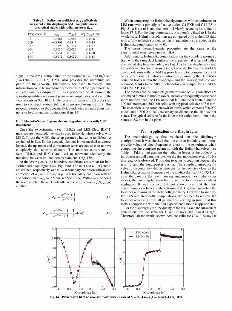
theoretical values with radiation losses Rrad

Frequency, Hz Rrad jRLESj arg�RLES�, rad77 −0.9984 1.0063 3.1408269 −0.9803 0.9847 3.1413387 −0.9596 0.9597 3.1727604 −0.9039 0.9029 3.1551757 −0.8534 0.8500 3.1438894 −0.8012 0.8022 3.1414

− 0.6 − 0.4 − 0.2 0.0 0.2 0.4X coordinate [m]

0.0

0.2

0.4

0.6

0.8

1.0

1.2

abs(

p)

− 0.6 − 0.4 − 0.2 0.0 0.2 0.4X coordinate [m]

0

1

2

3

4

5

arg(

p)

DMD Only

DMD + Fit

Fig. 14 Plane waves fit of an acoustic mode (swirler case at U � 0.34 m∕s, f � �284.9–13.2i� Hz).

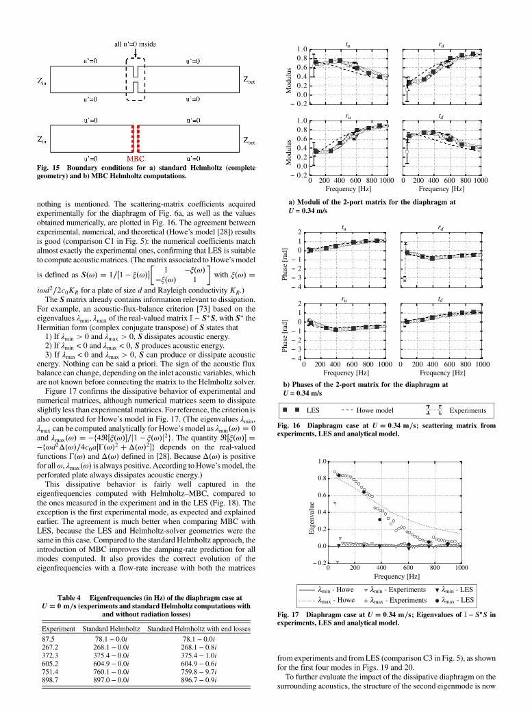
nothing is mentioned. The scattering-matrix coefficients acquiredexperimentally for the diaphragm of Fig. 6a, as well as the valuesobtained numerically, are plotted in Fig. 16. The agreement betweenexperimental, numerical, and theoretical (Howe’s model [28]) resultsis good (comparison C1 in Fig. 5): the numerical coefficients matchalmost exactly the experimental ones, confirming that LES is suitableto compute acousticmatrices. (Thematrix associated toHowe’smodel

is defined as S�ω� � 1∕�1 − ξ�ω���

1 −ξ�ω�−ξ�ω� 1

�with ξ�ω� �

iωd2∕2c0KR for a plate of size d and Rayleigh conductivity KR.)The Smatrix already contains information relevant to dissipation.

For example, an acoustic-flux-balance criterion [73] based on theeigenvalues λmin; λmax of the real-valued matrix I − S�S, with S� theHermitian form (complex conjugate transpose) of S states that1) If λmin > 0 and λmax > 0, S dissipates acoustic energy.2) If λmin < 0 and λmax < 0, S produces acoustic energy.3) If λmin < 0 and λmax > 0, S can produce or dissipate acoustic

energy. Nothing can be said a priori. The sign of the acoustic fluxbalance can change, depending on the inlet acoustic variables, whichare not known before connecting the matrix to the Helmholtz solver.Figure 17 confirms the dissipative behavior of experimental and

numerical matrices, although numerical matrices seem to dissipateslightly less than experimental matrices. For reference, the criterion isalso computed for Howe’s model in Fig. 17. (The eigenvalues λmin,λmax can be computed analytically for Howe’s model as λmin�ω� � 0and λmax�ω� � −f4R�ξ�ω��∕j1 − ξ�ω�j2g. The quantity R�ξ�ω�� �−fωd2Δ�ω�∕4c0a�Γ�ω�2 � Δ�ω�2�g depends on the real-valuedfunctions Γ�ω� and Δ�ω� defined in [28]. Because Δ�ω� is positivefor allω, λmax�ω� is always positive. According to Howe’smodel, theperforated plate always dissipates acoustic energy.)This dissipative behavior is fairly well captured in the

eigenfrequencies computed with Helmholtz–MBC, compared tothe ones measured in the experiment and in the LES (Fig. 18). Theexception is the first experimental mode, as expected and explainedearlier. The agreement is much better when comparing MBC withLES, because the LES and Helmholtz-solver geometries were thesame in this case. Compared to the standard Helmholtz approach, theintroduction of MBC improves the damping-rate prediction for allmodes computed. It also provides the correct evolution of theeigenfrequencies with a flow-rate increase with both the matrices

from experiments and fromLES (comparison C3 in Fig. 5), as shownfor the first four modes in Figs. 19 and 20.To further evaluate the impact of the dissipative diaphragm on the

surrounding acoustics, the structure of the second eigenmode is now

− 0.20.00.20.40.60.81.0

Mod

ulus

tu rd

Frequency [Hz]

− 0.20.00.20.40.60.81.0

Mod

ulus

ru

Frequency [Hz]

td

a) Moduli of the 2-port matrix for the diaphragm atU = 0.34 m/s

b) Phases of the 2-port matrix for the diaphragm atU = 0.34 m/s

− 4− 3− 2− 1

012

Phas

e[r

ad]

tu rd

Frequency [Hz]

− 4− 3− 2− 1

012

Phas

e[r

ad]

ru

0 200 400 600 800 1000

0 200 400 600 800 10000 200 400 600 800 1000

0 200 400 600 800 1000Frequency [Hz]

td

LES Howe model Experiments

Fig. 16 Diaphragm case at U � 0.34 m∕s; scattering matrix fromexperiments, LES and analytical model.

0 200 400 600 800 1000Frequency [Hz]

− 0.2

0.0

0.2

0.4

0.6

0.8

1.0

Eig

enva

lue

λmin - Howe

λmax - Howe

λmin - Experiments

λmax - Experiments

λmin - LES

λmax - LES

Fig. 17 Diaphragm case at U � 0.34 m∕s; Eigenvalues of I − S�S inexperiments, LES and analytical model.

Table 4 Eigenfrequencies (in Hz) of the diaphragm case at

U � 0 m∕s (experiments and standardHelmholtz computations withand without radiation losses)

Experiment Standard Helmholtz Standard Helmholtz with end losses

87.5 78.1 − 0.0i 78.1 − 0.0i267.2 268.1 − 0.0i 268.1 − 0.8i372.3 375.4 − 0.0i 375.4 − 1.0i605.2 604.9 − 0.0i 604.9 − 0.6i751.4 760.1 − 0.0i 759.8 − 9.7i898.7 897.0 − 0.0i 896.7 − 0.9i

Fig. 15 Boundary conditions for a) standard Helmholtz (completegeometry) and b) MBC Helmholtz computations.

compared between experiments, LES, and Helmholtz-solvercomputations. This is done by plotting the modulus and phase ofp, normalized at x � −0.58m. Both experiments (Fig. 21) and LES

(Fig. 22) show that the presence of a mean flow through thediaphragm modifies the pressure jump across the orifice, which is adirect indication of acoustic losses. This effect is captured by the

0 200 400 600 800 1000fr [Hz]

−40

−30

−20

−10

0

f i[H

z]

Standard Helmholtz

Helmholtz with MBC - Experimental matrix

Experiments

a) Helmholtz solver with MBC vs experiments(C2-EXP in Fig. 5)

0 200 400 600 800 1000fr [Hz]

−40

−30

−20

−10

0

f i[H

z]

Standard Helmholtz

Helmholtz with MBC - LES matrix

LES

b) Helmholtz solver with MBC vs LES (C2-LESin Fig. 5)

Fig. 18 Diaphragm case. Eigenfrequencies from standard and MBC Helmholtz vs a) experiments, b) LES.

0.15 0.20 0.25 0.30 0.3570

75

80

85

90

95

f r[H

z]

Mode 1

0.15 0.20 0.25 0.30 0.35260

265

270

275

280

285 Mode 2

0.15 0.20 0.25 0.30 0.35Inlet bulk velocity [m/s]

− 45− 40− 35− 30− 25− 20− 15− 10

f i[H

z]

0.15 0.20 0.25 0.30 0.35Inlet bulk velocity [m/s]

− 35− 30− 25− 20− 15− 10

− 50

Experiments

Helmholtz with MBC - Experimental matrixLES

Helmholtz with MBC - LES matrix

Fig. 19 Diaphragm case. Eigenfrequencies vs U (top: real part, bottom; imaginary part).

0.15 0.20 0.25 0.30 0.35365

370

375

380

385

390

f r[H

z]

Mode 3

0.15 0.20 0.25 0.30 0.35590

595

600

605

610

615 Mode 4

0.15 0.20 0.25 0.30 0.35Inlet bulk velocity [m/s]

− 35− 30− 25− 20− 15− 10− 5

0

f i[H

z]

0.15 0.20 0.25 0.30 0.35Inlet bulk velocity [m/s]

− 35− 30− 25− 20− 15− 10− 5

0

Experiments

Helmholtz with MBC - Experimental matrixLES

Helmholtz with MBC - LES matrix

Fig. 20 Diaphragm case. Eigenfrequencies vs U, continued (top: real part, bottom: imaginary part).

Helmholtz solver with MBC, but not by a standard Helmholtzcomputation (Figs. 21 and 22). These good results support our initialassumption that, at first order, the impact of mean flow is importantonly at locations where damping through vortex shedding is present,and can be neglected elsewhere, so that acoustics arewell representedby the zero-mean-flow Helmholtz equation (1).

V. Application to an Industrial Swirler

In the diaphragm configuration, the flow was laminar and fairlysimple: the only complexity was the shear layer created at thedownstream lips of the diaphragm.Moreover, the analytical model ofHowe [28] was available for comparison. Now, the methodology isapplied to the more challenging swirler element (Fig. 6b) for whichthere is no theoretical formula. Downstream of the swirler, the flowfeatures complex phenomena, such as recirculation zones orprecessing vortex cores. Because the comparison with the LES(C2-LES in Fig. 5) gave the best results for the diaphragm,it is the only comparison performed for the swirler. The LEScomputations were performed for the highest bulk velocity U �0.34 m∕s to maximize the acoustic–hydrodynamic coupling.Compared to the diaphragm case, the outlet is fully reflective bothin the LES and in the Helmholtz solver. Two modes are studied here:mode A and mode B with frequencies around 285 and 590 Hz,respectively, at U � 0.34 m∕s (as assessed by LES, Table 5). Theswirler matrix coefficients were computed at 280, 290, 370, and590 Hz, and are listed in Table 6, and linear interpolation is used toobtain the effective coefficients at the Helmholtz-solver frequency.With the exception of 370 Hz, which is used later to assess the errormade if the matrix is not measured at the correct frequency, the otherfrequencies were chosen close to the frequencies of mode A andmode B.

In Table 5, the results of the Helmholtz solver are comparedto the LES for mode A and mode B. In terms of damping rates, theMBC methodology captures the correct order of magnitude,contrary to the standard Helmholtz solver, which leads toωi � 0, asexpected. The relative error on the frequencies, computed asjfHelmholtz − fLES∕fLESj, remains around 1% for both modes.

X coordinate [m]

0.0

0.2

0.4

0.6

0.8

1.0

1.2

1.4

abs(

p)

−0.6 −0.4 −0.2 0.0 0.2 0.4−0.6 −0.4 −0.2 0.0 0.2 0.4X coordinate [m]

0.0

0.5

1.0

1.5

2.0

2.5

3.0

3.5

arg(

p)

Standard HelmholtzHelmholtz with MBC(Experimental matrix) Experiment

Fig. 21 Diaphragm case. Second eigenmode structure from experiments, standard and MBC Helmholtz computations.

0.0

0.2

0.4

0.6

0.8

1.0

1.2

1.4

0.0

0.5

1.0

1.5

2.0

2.5

3.0

3.5

Standard HelmholtzHelmholtz with MBC(LES matrix) LES

−0.6 −0.4 −0.2 0.0 0.2 0.4X coordinate [m]

−0.6 −0.4 −0.2 0.0 0.2 0.4X coordinate [m]

abs(

p)

arg(

p)

Fig. 22 Diaphragm case. Third mode structure from LES, standard and MBC Helmholtz computations.

Table 5 Complex frequencies (inHz) ofmodeA andmode Bwith theswirler at U � 0.34 m∕s, from LES, Helmholtz solver with LES matrix,

and standard Helmholtz solver

Mode A Mode B

Standard Helmholtz 317.4 − 0.0i 591.2 − 0.0iLES 284.9 − 13.2i 589.1 − 3.2iHelmholtz with LES matrix 287.5 − 13.7i 597.7 − 1.3iRelative error, % 0.9 1.5

The relative difference between Helmholtz and LES results is also displayed.

Table 6 Swirler matrix

280 Hz 290 Hz 370 Hz 590 Hz

tu 0.189�0.002 0.268 − 0.054j 0.465�0.043j 0.043�0.117jrd 0.833�0.099j 0.775�0.076j 0.568�0.203j 0.946�0.012jru 0.806�0.079j 0.712�0.094j 0.538�0.033j 0.955�0.001jtd 0.170 − 0.014j 0.217�0.005j 0.392 − 0.079j 0.034�0.196jλmin −0.006 0.016 0.003 −0.038λmax 0.582 0.741 0.965 0.176

Scattering-matrix coefficients from LES forU � 0.34 m∕s and eigenvalues of I − S�S.

The eigenmode structures are also well retrieved by the MBCapproach, as illustrated in Figs. 23 and 24.In a general case with turbulent complex flow, as is the case with

the swirler, it can be difficult to properly separate acousticfluctuations from hydrodynamic ones. This results in uncertainties inthe acoustic matrix coefficients. Moreover, the frequencies of themodes of interest are not always available beforehand. In this case,thematrix can bemeasured for a chosen set of frequencies, and linearinterpolation is applied to retrieve the coefficients at the desiredfrequency, as was done here. This introduces an additionaluncertainty. To assess the effect of these uncertainties on the result ofthe MBC–Helmholtz methodology, 50 additional Helmholtzcomputations are performed for mode A by varying the coefficientsof the scattering matrix as follows. Each coefficient can have fivedifferent values: the nominal value, the nominal value plus ΔS, thenominal value minus ΔS, the nominal value plus jΔS, and thenominal value minus jΔS. The total number of matrix combinationsamounts to 695, among which 50 combinations are sampledrandomly.ΔS is a real number chosen arbitrarily to 0.03, and accountsfor the uncertainty on the matrix due to the measurement method, butalso on the frequency at whichmeasurements are taken. Variations ofthe order of ΔS on the scattering matrix were observed wheninterpolating the matrix between 280 and 290 Hz instead of 280 and370 Hz (Table 6).Figure 25 shows that the complex eigenfrequency computed

withMBC–Helmholtz is indeed sensitive to the value of the matrixcoefficients (the nominal result is recalled in Fig. 25 as a whitesquare). In particular, the variations of the imaginary part of thefrequency can reach up to 3.5 Hz, corresponding to approximately

25% of the nominal value. The eigenmode structure is also greatlyimpacted (Fig. 26). In Fig. 26, the normalization is different fromthat used in Fig. 23, because fixing p � 1 at x � −0.58 m wouldforce all modes to collapse in the upstream section. To better seethe changes in both upstream and downstream mode structures, pis fixed to 1 at x � 0, the matrix location. The great dispersion ofmode shapes around the nominal result in black suggests that thematrices should be carefully measured to obtain satisfying resultswith the MBC methodology. In our experience, the biggest source

X coordinate [m]

0.0

0.2

0.4

0.6

0.8

1.0

1.2

abs(

p)

X coordinate [m]

−1

0

1

2

3

4

5

Standard HelmholtzHelmholtz with MBC(LES matrix) LES

−0.6 −0.4 −0.2 0.0 0.2 0.4−0.6 −0.4 −0.2 0.0 0.2 0.4

arg(

p)

Fig. 23 Swirler case. Structure of mode A from LES, standard and MBC Helmholtz computations.

X coordinate [m]

0.0

0.2

0.4

0.6

0.8

1.0

1.2

abs

(p

)

X coordinate [m]

−1

0

1

2

3

4

5

arg

(p

)

Standard HelmholtzHelmholtz with MBC(LES matrix) LES

−0.6 −0.4 −0.2 0.0 0.2 0.4−0.6 −0.4 −0.2 0.0 0.2 0.4

Fig. 24 Swirler case. Structure of mode B from LES, standard and MBC Helmholtz computations.

279.00 282.51 286.02 289.53 293.04fr [Hz]

-21.44

-17.93

-14.42

-10.91

-7.41

f i[H

z]

Fig. 25 Swirler case. Sensitivity of the frequency of mode A to matrixcoefficients.

of error is the frequency of measurement, which should ideally bechosen as close as possible to the frequency of the mode foundby AVSP.

VI. Conclusions

A methodology was presented to describe the acousticbehavior of non-purely acoustic elements in a zero-mean-flowHelmholtz solver. Compared to other approaches, such as LNSE,it has the advantage of being slightly faster and compatible withthe prediction of thermoacoustic instabilities (although noinstability was investigated in this paper). Here, the elements ofinterest are represented by their two-port matrix, introduced inthe Helmholtz solver, thanks to an MBC. The methodology wasapplied on an academic configuration to retrieve the dissipativeeffects of two elements: a diaphragm and a swirler. For theseelements, the acoustic–hydrodynamic interaction was the sourceof important damping rates and changes in the eigenmodestructures. These modifications were correctly captured by theHelmholtz solver with MBC, with matrices measured numeri-cally and experimentally, whereas the standard Helmholtzsolution misses them. However, a simple sensitivity analysisshowed that the matrix should be carefully measured to obtainmeaningful results. In particular, the frequency at which thematrix is measured should be as close as possible to thefrequency of the mode of interest.

Appendix A: Howe’s Model for the Acoustic Dampingof a Perforated Plate

Howe [28] derived a model to account for the acoustic dampingcreated by a perforated plate. Across the plate, the acoustic pressure pis discontinuous, whereas the acoustic volume-flow rate G � d2u ·n is conserved; d is the average distance between perforations, seeFig. A1. This creates a difference between the inlet acoustic flux1∕2R�p�G�� and the outlet acoustic flux 1∕2R�p−G��, whichcorresponds to the flux dissipated at the plate. The flux difference isdirectly controlled by a quantity known as the Rayleigh conductivity[32]. The Rayleigh conductivity KR quantifies the ratio of the

acoustic-pressure jump over the acoustic volume-flow rate [4], andwas derived analytically by Howe [28] for perforated plates. For theplate of Fig. A1

KR � iρoωG

�p� − p−� � 2a�ΓSr − iΔSr� (A1)

in which a is the radius of the perforations (assumed of cylindricalshape), and ΓSr andΔSr are two real valued functions of the Strouhalnumber given in [28]. The Strouhal number is definedwith the orificebias speed as Sr � ωa∕Uori.Howe’s model can also be used to compute the Rayleigh

conductivity of one perforation in a circular plate. In this case, theaverage distance between perforations d is replaced by

π

pR, with R

the radius of the plate.

Appendix B: Numerical Parameters for LESComputations

All CFD computations are performed with the LES solver AVBP[60], codeveloped byCERFACS and IFPEN. This tool is widely usedand has beenvalidated in numerous situations [15,18,30,61–64]. Thenumerical scheme two-step Taylor-Galerkin C is third-order accuratein time and space, andwas specifically designed to properly representunsteady compressible flows with or without combustion [65]. The σmodel [66,67] is used to model the subgrid-scale stress tensoraccurately.For all computations, the diaphragm and swirler parts are modeled

as adiabatic no-slipwalls, whereas the ductwalls are representedwithadiabatic slip conditions. The acoustic losses due to shear stress orthermal diffusion in the main duct are therefore neglected. As said inthe Introduction, this is because this effect is small compared toacoustic–hydrodynamic damping in the low-frequency range.

Characteristic Navier–Stokes inlet and outlet boundary conditions[68] are used for pulsed computations. For AMT computations, theinlet and outlet are switched to completely reflecting boundaries, soas to measure the damping rate associated with the diaphragm orswirler, and not the one due to losses at boundaries.

− 0.6 − 0.4 − 0.2 0.0 0 .2 0 .4X coordinate [m]

0.0

0.2

0.4

0.6

0.8

1.0

1.2

1.4

1.6

abs(

p)

− 0.6 − 0.4 − 0.2 0.0 0 .2 0 .4X coordinate [m]

− 4

− 3

− 2

− 1

0

1

arg

(p)

Fig. 26 Swirler case. Sensitivity of the structure of mode A to matrix coefficients.

2a

Uori

d

d

Fig. A1 Quantities used in Howe’s model.

Acknowledgments

The authors wish to thank A. Misdariis for performing thestationary large-eddy-simulation computations used as a startingpoint for this analysis, and M. Bauerheim for the fruitful discussionsabout acoustic-mode triggering. The experiments were performedwith the funding from the European Research Council (ERC) underthe European Union’s Seventh Framework Programme (FP/2007-2013)/ERC grant agreement ERC-AdG 319067-INTECOCIS. Thesupport from A. Cayre and S. Roux at Safran–Société Nationaled’Etude et de Construction de Moteurs d’Aviation is also gratefullyacknowledged.

References

[1] Candel, S., Durox, D., Schuller, T., Bourgouin, J.-F., and Moeck, J. P.,“Dynamics of Swirling Flames,” Annual Review of Fluid Mechanics,Vol. 46, No. 1, Jan. 2014, pp. 147–173.doi:10.1146/annurev-fluid-010313-141300

[2] Culick, F. E. C., and Kuentzmann, P., “Unsteady Motions inCombustion Chambers for Propulsion Systems,” NATO Research andTechnology Organisation AG-AVT-039, Neuilly-sur-Seine, France,2006.

[3] Lieuwen, T. C., Unsteady Combustor Physics, Cambridge Univ. Press,Cambridge, 2012.doi:10.1017/cbo9781139059961

[4] Rayleigh, L., The Theory of Sound, Macmillan, London, 1894, pp. 226–234 (reprinted by Dover, New York, 1945).

[5] Candel, S., “Combustion Dynamics and Control: Progress andChallenges,” Proceedings of the Combustion Institute, Vol. 29, No. 1,Jan. 2002, pp. 1–28.doi:10.1016/S1540-7489(02)80007-4

[6] Lieuwen, T., and Yang, V., Combustion Instabilities in Gas Turbine

Engines: Operational Experience, Fundamental Mechanisms, and

Modeling, Vol. 210, Progress in Astronautics and Aeronautics, AIAA,Reston, VA, 2005.

[7] Evesque, S., and Polifke, W., “Low-Order Acoustic Modelling forAnnular Combustors: Validation and Inclusion of Modal Coupling,”ASME Turbo Expo 2002: Power for Land, Sea, and Air, ASMEInternational, New York, 2002, pp. 321–331.doi:10.1115/gt2002-30064

[8] Schuermans, B., Bellucci, V., and Paschereit, C. O., “ThermoacousticModeling and Control of Multi Burner Combustion Systems,” ASME

Turbo Expo 2003, ASME International, New York, 2003, pp. 509–519.doi:10.1115/gt2003-38688

[9] Stow, S. R., and Dowling, A. P., “Low-Order Modelling ofThermoacoustic Limit Cycles,” ASME Turbo Expo 2004: Power for

Land, Sea, andAir, ASME International, NewYork, 2004, pp. 775–786.doi:10.1115/gt2004-54245

[10] Bauerheim,M., Parmentier, J., Salas, P., Nicoud, F., and Poinsot, T., “AnAnalytical Model for Azimuthal Thermoacoustic Modes in an AnnularChamber Fed by anAnnular Plenum,”Combustion andFlame, Vol. 161,No. 5, May 2014, pp. 1374–1389.doi:10.1016/j.combustflame.2013.11.014

[11] Han, X., Li, J., and Morgans, A. S., “Prediction of CombustionInstability Limit Cycle Oscillations by Combining Flame DescribingFunction Simulations with a Thermoacoustic Network Model,”Combustion and Flame, Vol. 162, No. 10, Oct. 2015, pp. 3632–3647.doi:10.1016/j.combustflame.2015.06.020

[12] Huang, Y., Sung, H. G., Hsieh, S. Y., and Yang, V., “Large EddySimulation of Combustion Dynamics of Lean-Premixed Swirl-Stabilized Combustor,” Journal of Propulsion and Power, Vol. 19,No. 5, Nov. 2003, pp. 782–794.doi:10.2514/2.6194

[13] Schmitt, P., Poinsot, T., Schuermans, B., andGeigle, K. P., “Large-EddySimulation and Experimental Study of Heat Transfer, Nitric OxideEmissions and Combustion Instability in a Swirled Turbulent High-Pressure Burner,” Journal of Fluid Mechanics, Vol. 570, Jan. 2007,pp. 17–46.doi:10.1017/S0022112006003156

[14] Staffelbach, G., Gicquel, L., Boudier, G., and Poinsot, T., “Large EddySimulation of Self-Excited Azimuthal Modes in Annular Combustors,”Proceedings of the Combustion Institute, Vol. 32, No. 2, 2009,pp. 2909–2916.doi:10.1016/j.proci.2008.05.033

[15] Wolf, P., Staffelbach, G., Gicquel, L., Muller, J.-D., and Poinsot, T.,“Acoustic and Large Eddy Simulation Studies of Azimuthal Modes inAnnular Combustion Chambers,” Combustion and Flame, Vol. 159,

No. 11, Nov. 2012, pp. 3398–3413.doi:10.1016/j.combustflame.2012.06.016

[16] Gicquel, L. Y. M., Staffelbach, G., and Poinsot, T., “Large EddySimulations ofGaseous Flames inGasTurbineCombustionChambers,”Progress in Energy and Combustion Science, Vol. 38, No. 6, 2012,pp. 782–817.doi:10.1016/j.pecs.2012.04.004

[17] Hermeth, S., Staffelbach, G., Gicquel, L., and Poinsot, T., “LESEvaluation of the Effects of Equivalence Ratio Fluctuations on theDynamic Flame Response in a Real Gas Turbine CombustionChamber,” Proceedings of the Combustion Institute, Vol. 34, No. 2,2013, pp. 3165–3173.doi:10.1016/j.proci.2012.07.013

[18] Ghani, A., Poinsot, T., Gicquel, L., and Staffelbach, G., “LES ofLongitudinal and Transverse Self-Excited Combustion Instabilities in aBluff-Body Stabilized Turbulent Premixed Flame,” Combustion and

Flame, Vol. 162, No. 11, Nov. 2015, pp. 4075–4083.doi:10.1016/j.combustflame.2015.08.024

[19] Kierkegaard, A., Boij, S., and Efraimsson, G., “Simulations of theScattering of Sound Waves at a Sudden Area Expansion,” Journal of

Sound and Vibration, Vol. 331, No. 5, 2012, pp. 1068–1083.doi:10.1016/j.jsv.2011.09.011

[20] Kierkegaard, A., Allam, S., Efraimsson, G., and Åbom, M.,“Simulations of Whistling and the Whistling Potentiality of anIn-Duct Orifice with Linear Aeroacoustics,” Journal of Sound and

Vibration, Vol. 331, No. 5, Feb. 2012, pp. 1084–1096.doi:10.1016/j.jsv.2011.10.028

[21] Gikadi, J., Ullrich,W. C., Sattelmayer, T., and Turrini, F., “Prediction ofthe Acoustic Losses of a Swirl Atomizer Nozzle Under Non-ReactiveConditions,” ASME Turbo Expo 2013: Turbine Technical Conference

and Exposition, American Soc. of Mechanical Engineers PaperV01BT04A035, New York, June 2013.doi:10.1115/gt2013-95449

[22] Stokes, G. G., “On the Effect of the Inertial Friction of Fluids on theMotions of Pendulums,” Transactions of the Cambridge PhilosophicalSociety, Vol. 9, 1851, pp. 8–23.doi:10.1017/cbo9780511702266.002

[23] Kirchhoff, G., “Ueber den Einfluss derWärmeleitung in einemGase aufdie Schallbewegung,” Annalen der Physik, Vol. 210, No. 6, 1868,pp. 177–193.doi:10.1002/(ISSN)1521-3889

[24] Nielsen,A.K., “AcousticResonators ofCircularCross-Section andwithAxial Symmetry,” Transactions of the Danish Academy of Technical

Sciences, Vol. 10, 1949, pp. 9–70[25] Searby, G., Nicole, A., Habiballah, M., and Laroche, E., “Prediction of

the Efficiency of Acoustic Damping Cavities,” Journal of Propulsionand Power, Vol. 24, No. 3, May 2008, pp. 516–523.doi:10.2514/1.32325

[26] Temkin, S., and Dobbins, R. A., “Attenuation and Dispersion of Soundby Particulate-Relaxation Processes,” Journal of the Acoustical Societyof America, Vol. 40, No. 2, 1966, p. 317.doi:10.1121/1.1910073

[27] Williams, F.A.,CombustionTheory, BenjaminCummings,Menlo Park,CA, 1985, pp. 304–315.

[28] Howe,M. S., “On the Theory ofUnsteadyHighReynoldsNumber FlowThrough a Circular Aperture,” Proceedings of the Royal Society of

London, Series A: Mathematical, Physical and Engineering Sciences,Vol. 366, No. 1725, June 1979, pp. 205–223.doi:10.1098/rspa.1979.0048

[29] Jing, X., and Sun, X., “Effect of Plate Thickness on Impedance ofPerforated Plates with Bias Flow,” AIAA Journal, Vol. 38, No. 9,Jan. 2000, pp. 1573–1578.doi:10.2514/2.1139

[30] Mendez, S., and Eldredge, J., “Acoustic Modeling of Perforated PlateswithBias Flow for Large-Eddy Simulations,” Journal of ComputationalPhysics, Vol. 228, No. 13, July 2009, pp. 4757–4772.doi:10.1016/j.jcp.2009.03.026

[31] Tam, C. K. W., Ju, H., Jones, M. G., Watson, W. R., and Parrott, T. L.,“A Computational and Experimental Study of Resonators in ThreeDimensions,” Journal of Sound and Vibration, Vol. 329, No. 24,Nov. 2010, pp. 5164–5193.doi:10.1016/j.jsv.2010.06.005

[32] Gullaud, E., and Nicoud, F., “Effect of Perforated Plates on theAcoustics of Annular Combustors,” AIAA Journal, Vol. 50, No. 12,Dec. 2012, pp. 2629–2642.doi:10.2514/1.J050716

[33] Scarpato, A., Tran, N., Ducruix, S., and Schuller, T., “Modeling theDamping Properties of Perforated Screens Traversed by aBias Flow andBacked by a Cavity at Low Strouhal Number,” Journal of Sound and

Vibration, Vol. 331, No. 2, 2012, pp. 276–290.doi:10.1016/j.jsv.2011.09.005

[34] Fischer, A., Hirsch, C., and Sattelmayer, T., “Comparison of Multi-Microphone Transfer Matrix Measurements with Acoustic NetworkModels of Swirl Burners,” Journal of Sound and Vibration, Vol. 298,Nos. 1–2, Nov. 2006, pp. 73–83.doi:10.1016/j.jsv.2006.04.040

[35] Föller, S., Polifke, W., and Tonon, D., “Aeroacoustic Characterizationof T-Junctions Based on Large Eddy Simulation and SystemIdentification,” 16th AIAA/CEAS Aeroacoustics Conference, AIAAPaper 2010-3985, June 2010.doi:10.2514/6.2010-3985

[36] Karlsson, M., and Åbom, M., “Quasi-Steady Model of the AcousticScattering Properties of a T-Junction,” Journal of Sound and Vibration,Vol. 330, No. 21, 2011, pp. 5131–5137.doi:10.1016/j.jsv.2011.05.012

[37] Howe,M., “TheDissipation of Sound at an Edge,” Journal of Sound andVibration, Vol. 70, No. 3, June 1980, pp. 407–411.doi:10.1016/0022-460X(80)90308-9

[38] Tam, C. K. W., Ju, H., Jones, M. G., Watson, W. R., and Parrott, T. L.,“A Computational and Experimental Study of Slit Resonators,”Journal of Sound and Vibration, Vol. 284, No. 3, June 2005,pp. 947–984.doi:10.1016/j.jsv.2004.07.013

[39] Rienstra, S. W., and Hirschberg, A., An Introduction to Acoustics,Eindhoven Univ. of Technology, Eindhoven, 2003, pp. 30–32, 68–70.

[40] Åbom, M., “Measurement of the Scattering-Matrix of AcousticalTwo-Ports,”Mechanical Systems and Signal Processing, Vol. 5, No. 2,March 1991, pp. 89–104.doi:10.1016/0888-3270(91)90017-Y

[41] Paschereit, C. O., Polifke, W., Schuermans, B., and Mattson, O.,“Measurement of Transfer Matrices and Source Terms of PremixedFlames,” Journal of Engineering forGas Turbines and Power, Vol. 124,No. 2, 2002, pp. 239–247.doi:10.1115/1.1383255

[42] Polifke, W., Poncet, A., Paschereit, C. O., and Doebbeling, K.,“Reconstruction of Acoustic Transfer Matrices by InstationaryComputational Fluid Dynamics,” Journal of Sound and Vibration,Vol. 245, No. 3, Aug. 2001, pp. 483–510.doi:10.1006/jsvi.2001.3594

[43] Munjal,M. L.,Acoustics of Ducts andMufflers,Wiley,NewYork, 1986,pp. 75–85, 121–147.

[44] Gentemann, A., Fischer, A., Evesque, S., and Polifke, W., “AcousticTransfer Matrix Reconstruction and Analysis for Ducts with SuddenChange of Area,” 9th AIAA/CEAS Aeroacoustics Conference, AIAAPaper 2003-3142, May 2003.doi:10.2514/6.2003-3142

[45] Föller, S., and Polifke, W., “Identification of Aero-Acoustic ScatteringMatrices from Large Eddy Simulation: Application to a Sudden AreaExpansion of aDuct,” Journal of Sound andVibration, Vol. 331,No. 13,June 2012, pp. 3096–3113.doi:10.1016/j.jsv.2012.01.004

[46] Polifke, W., and Paschereit, C. O., “Determination of Thermo-AcousticTransfer Matrices by Experiment and Computational Fluid Dynamics,”ERCOFTAC Bulletin, 1998, p. 38.

[47] Truffin, K., and Poinsot, T., “Comparison and Extension ofMethods forAcoustic Identification of Burners,” Combustion and Flame, Vol. 142,No. 4, Sept. 2005, pp. 388–400.doi:10.1016/j.combustflame.2005.04.001

[48] Bomberg, S., Emmert, T., and Polifke, W., “Thermal Versus AcousticResponse of Velocity Sensitive Premixed Flames,” Proceedings of theCombustion Institute, Vol. 35, No. 3, 2015, pp. 3185–3192.doi:10.1016/j.proci.2014.07.032

[49] Strobio Chen, L., Witte, A., and Polifke, W., “Thermo-AcousticCharacterization of a Heat Exchanger in Cross Flow UsingCompressible and Weakly Compressible Numerical Simulation,”22nd International Congress on Sound and Vibration (ICSV22),ICSV, Acoustical Soc. of Italy, July 2015, Paper 477, http://iiav.org/icsv22.

[50] Jaensch, S., Emmert, T., Silva, C., and Polifke, W., “A Grey-BoxIdentification Approach for Thermoacoustic Network Models,” ASME

Turbo Expo 2014: Turbine Technical Conference and Exposition,American Soc. of Mechanical Engineers Paper V04BT04A051, NewYork, June 2014.doi:10.1115/gt2014-27034

[51] Bourgouin, J. F., Durox, D., Moeck, J. P., Schuller, T., and Candel, S.,“Characterization and Modeling of a Spinning ThermoacousticInstability in an Annular Combustor Equipped with Multiple MatrixInjectors,” Journal of Engineering for Gas Turbines and Power,

Vol. 137, No. 2, June 2015, Paper 021503.doi:10.1115/gt2014-25067

[52] Campa, G., and Camporeale, S., “Eigenmode Analysis of theThermoacoustic Combustion Instabilities Using a Hybrid TechniqueBased on the Finite Element Method and the Transfer Matrix Method,”Advances in Applied Acoustics, Vol. 1, No. 1, 2012, pp. 1–14.

[53] Laera, D., Gentile, A., Camporeale, S. M., Bertolotto, E., Rofi, L., andBonzani, F., “Numerical and Experimental Investigation of Thermo-Acoustic Combustion Instability in a Longitudinal CombustionChamber: Influence of the Geometry of the Plenum,” ASME Turbo

Expo 2015: Turbine Technical Conference and Exposition, AmericanSoc. of Mechanical Engineers Paper V04AT04A028, June 2015.doi:10.1115/gt2015-42322

[54] Nicoud, F., Benoit, L., Sensiau, C., and Poinsot, T., “AcousticModes inCombustors with Complex Impedances and Multidimensional ActiveFlames,” AIAA Journal, Vol. 45, No. 2, Feb. 2007, pp. 426–441.doi:10.2514/1.24933

[55] Poinsot, T., Chatelier, T. L., Candel, S., and Esposito, E., “ExperimentalDetermination of the Reflection Coefficient of a Premixed Flamein a Duct,” Journal of Sound and Vibration, Vol. 107, No. 2, 1986,pp. 265–278.doi:10.1016/0022-460X(86)90237-3

[56] Noiray, N., and Schuermans, B., “Deterministic Quantities Character-izing Noise Driven Hopf Bifurcations in Gas Turbine Combustors,”International Journal of Non-Linear Mechanics, Vol. 50, April 2013,pp. 152–163.doi:10.1016/j.ijnonlinmec.2012.11.008

[57] Silva, C. F., Nicoud, F., Schuller, T., Durox, D., and Candel, S.,“Combining a Helmholtz Solver with the Flame Describing Function toAssess Combustion Instability in a Premixed Swirled Combustor,”Combustion and Flame, Vol. 160, No. 9, Sept. 2013, pp. 1743–1754.doi:10.1016/j.combustflame.2013.03.020

[58] Palies, P., Durox, D., Schuller, T., and Candel, S., “NonlinearCombustion Instability Analysis Based on the Flame DescribingFunctionApplied to Turbulent Premixed Swirling Flames,”Combustionand Flame, Vol. 158, No. 10, 2011, pp. 1980–1991.doi:10.1016/j.combustflame.2011.02.012

[59] Holmberg, A., Åbom, M., and Bodén, H., “Accurate ExperimentalTwo-Port Analysis of Flow Generated Sound,” Journal of Sound and

Vibration, Vol. 330, No. 26, Dec. 2011, pp. 6336–6354.doi:10.1016/j.jsv.2011.07.041

[60] Schönfeld, T., “Steady and Unsteady Flow Simulations Using theHybrid Flow Solver AVBP,” AIAA Journal, Vol. 37, Jan. 1999,pp. 1378–1385.doi:10.2514/3.14333

[61] Selle, L., Lartigue, G., Poinsot, T., Koch, R., Schildmacher, K.-U.,Krebs, W., Prade, B., Kaufmann, P., and Veynante, D., “CompressibleLarge EddySimulation of Turbulent Combustion inComplexGeometryon Unstructured Meshes,” Combustion and Flame, Vol. 137, No. 4,2004, pp. 489–505.doi:10.1016/j.combustflame.2004.03.008

[62] Mendez, S., and Nicoud, F., “Large-Eddy Simulation of a Bi-PeriodicTurbulent Flow with Effusion,” Journal of Fluid Mechanics, Vol. 598,March 2008, pp. 27–65.doi:10.1017/S0022112007009664

[63] Duran, I., Leyko, M., Moreau, S., Nicoud, F., and Poinsot, T.,“ComputingCombustion Noise by Combining Large Eddy Simulationswith Analytical Models for the Propagation of Waves Through TurbineBlades,” Comptes Rendus de l’Académie des Sciences, Series IIB:

Mécanique, Vol. 341, Nos. 1–2, Jan. 2013, pp. 131–140.doi:10.1016/j.crme.2012.10.012

[64] Motheau, E., Nicoud, F., and Poinsot, T., “Mixed Acoustic–EntropyCombustion Instabilities in Gas Turbines,” Journal of Fluid Mechanics,Vol. 749, June 2014, pp. 542–576.doi:10.1017/jfm.2014.245

[65] Colin, O., and Rudgyard, M., “Development of High-Order Taylor–Galerkin Schemes for Unsteady Calculations,” Journal of Computa-

tional Physics, Vol. 162, No. 2, 2000, pp. 338–371.doi:10.1006/jcph.2000.6538

[66] Nicoud, F., Baya Toda, H., Cabrit, O., Bose, S., and Lee, J., “UsingSingular Values to Build a Subgrid-Scale Model for Large EddySimulations,” Physics of Fluids, Vol. 23, No. 8, 2011, Paper 085106.doi:10.1063/1.3623274

[67] Baya Toda, H., Cabrit, O., Truffin, K., Bruneaux, G., and Nicoud, F.,“Assessment of Subgrid-Scale Models with a Large-Eddy Simulation-Dedicated Experimental Database: The Pulsatile Impinging Jet inTurbulent Cross-Flow,” Physics of Fluids, Vol. 26, No. 7, July 2014,Paper 075108.doi:10.1063/1.4890855

[68] Poinsot, T., and Lele, S., “Boundary Conditions for Direct Simulationsof Compressible Viscous Flows,” Journal of Computational Physics,Vol. 101, No. 1, 1992, pp. 104–129.doi:10.1016/0021-9991(92)90046-2

[69] Paschereit, C. O., and Polifke, W., “Characterization of Lean PremixedGas-Turbine Burners asAcousticMulti-Ports,”Bulletin of the AmericanPhysical Society/Division of Fluid Dynamics, Annual Meeting, SanFrancisco, CA, 1997.

[70] Bauerheim, M., “Theoretical and Numerical Study of SymmetryBreaking Effects on Azimuthal Thermoacoustic Modes in AnnularCombustors,” Ph.D. Thesis, Institut National Polytechnique deToulouse, Toulouse, 2014.

[71] Levine, H., and Schwinger, J., “On the Radiation of Sound from anUnflanged Circular Pipe,” Physical Review, Vol. 73, No. 4, Feb. 1948,

pp. 383–406.doi:10.1103/PhysRev.73.383

[72] Schmid, P. J., “Dynamic Mode Decomposition of Numerical andExperimental Data,” Journal of Fluid Mechanics, Vol. 656, July 2010,pp. 5–28.doi:10.1017/S0022112010001217

[73] Aurégan, Y., and Starobinski, R., “Determination of Acoustical EnergyDissipation/Production Potentiality from the Acoustical TransferFunctions of a Multiport,” Acta Acustica United with Acustica, Vol. 85,No. 6, 1999, pp. 788–792.