fastalgorithmsforhelmholtzgreen’sfunctions · fastalgorithmsforhelmholtzgreen’sfunctions ... of...

Fast algorithms for Helmholtz Green’s functions

BY GREGORY BEYLKIN*, CHRISTOPHER KURCZ AND LUCAS MONZON

Department of Applied Mathematics, University of Colorado at Boulder,526 UCB, Boulder, CO 80309-0526, USA

The formal representation of the quasi-periodic Helmholtz Green’s function obtained bythe method of images is only conditionally convergent and, thus, requires an appropriatesummation convention for its evaluation. Instead of using this formal sum, we derive acandidate Green’s function as a sum of two rapidly convergent series, one to be applied inthe spatial domain and the other in the Fourier domain (as in Ewald’s method). We provethat this representation of Green’s function satisfies the Helmholtz equation with thequasi-periodic condition and, furthermore, leads to a fast algorithm for its application asan operator.We approximate the spatial series by a short sum of separable functions given by

Gaussians in each variable. For the series in the Fourier domain, we exploit theexponential decay of its terms to truncate it. We use fast and accurate algorithms forconvolving functions with this approximation of the quasi-periodic Green’s function. Theresulting method yields a fast solver for the Helmholtz equation with the quasi-periodicboundary condition. The algorithm is adaptive in the spatial domain and its performancedoes not significantly deteriorate when Green’s function is applied to discontinuousfunctions or potentials with singularities. We also construct Helmholtz Green’s functionswith Dirichlet, Neumann or mixed boundary conditions on simple domains and use amodification of the fast algorithm for the quasi-periodic Green’s function to apply them.The complexity, in dimension dR2, of these algorithms is O(kd log kCC(log eK1)d),

where e is the desired accuracy, k is proportional to the number of wavelengths contained inthe computational domain and C is a constant. We illustrate our approach with examples.

Keywords: quasi-periodic Green’s functions;Dirichlet and Neumann boundary conditions; fast adaptive solvers; lattice sums;

separated representations; unequally spaced fast Fourier transform

*A

RecAcc

1. Introduction

In this paper, we construct fast and accurate algorithms for applying HelmholtzGreen’s functions incorporating a variety of boundary conditions on simpledomains. We come to this problem from the perspective of developing fastalgorithms for applying operators of mathematical physics with finite butarbitrary accuracy (in operator norm) as we discuss later. Instead of emphasizingcomputing of values of Green’s functions, as is typical in the literature mentionedbelow, we focus on the problem of applying such Green’s functions as operators

Proc. R. Soc. A (2008) 464, 3301–3326

doi:10.1098/rspa.2008.0161

Published online 26 August 2008

uthor for correspondence ([email protected]).

eived 18 April 2008epted 22 July 2008 3301 This journal is q 2008 The Royal Society

G. Beylkin et al.3302

in a fast and accurate manner. We note that the accurate computation of thevalues of a Green’s function does not by itself resolve the issue of its efficientapplication and use as an operator. Towards this end, we develop approxi-mations of Green’s functions that resolve the problem of algorithmic efficiency inapplying them to discontinuous functions or potentials with singularities.

The key element of our approach is a fast algorithm for computingconvolutions with the quasi-periodic Helmholtz Green’s function,

uðxÞZðDGqðxKyÞf ðyÞ dy; ð1:1Þ

for functions f 2LpðDÞ, where D is the primitive cell of a Bravais lattice L. Weconsider the case where the lattice is defined by d linearly independent vectors indimension dR2. Green’s function Gq satisfies

ðDCk2ÞGqðxÞZKdðxÞ; ð1:2Þ

GqðxC lÞZ eKik$lGqðxÞ; ð1:3Þ

where kO0, l2L, x2D and k2Rd. The quasi-periodicity vector k is sometimes

referred to as Bloch or crystal momentum vector. Consequently, the function uin (1.1) satisfies

ðDCk2ÞuðxÞZKf ðxÞ; ð1:4Þ

uðxC lÞZ eKik$luðxÞ: ð1:5Þ

It is well known that the method of images (typically used in dimensions dZ2or 3) gives rise to a natural, yet formal representation,

Gformalq ðxÞZ

1

4p

Xl2L

eikjxClj

jxC lj eik$l ; for dimension d Z 3;

i

4

Xl2L

Hð1Þ0 ðkjxC ljÞeik$l; for dimension d Z 2;

8>>>><>>>>:

ð1:6Þ

where j$j denotes the length of a vector and Hð1Þ0 is the zeroth-order Hankel

function of the first kind. These sums are only conditionally convergent; thus,they require a summation convention to yield a classical solution of (1.4)and (1.5).

The formal sum (1.6) appears in many areas of physics and engineering. Forexample, one of the first applications (Ewald (1913), see Cruickshank et al.(1992) for an English translation) describes X-ray diffraction by crystals using(1.6) as the key mathematical object. In fact, by transforming (1.6) to theFourier domain, it is easy to obtain directions and X-ray frequencies by usingthe so-called Ewald’s sphere. The sum (1.6) occurs in wave propagation inperiodic structures (e.g. Brillouin 1953), in the study of photonic crystals (e.g.Soukoulis 1992; Joannopoulos et al. 1995), in band structure computations insolid-state physics (e.g. Kohn & Rostoker 1954; Ham & Segall 1961), as well asin the analysis of ergodic systems (Berry 1981).

Proc. R. Soc. A (2008)

3303Fast algorithms for Green’s functions

Besides Ewald’s (1921) method, there are other approaches for interpretingand evaluating (1.6) (see Glasser & Zucker (1980) and Linton (1998) for a surveyand references therein). One approach is to use addition theorems for Besselfunctions, which separates the input variables x from the lattice vectors l. In suchcases, Green’s function is written as an expansion with respect to Besselfunctions with coefficients given by a lattice sum. We note that Yasumoto &Yoshitomi (1999), McPhedran et al. (2000) and Dienstfrey et al. (2001) employthis approach and develop different algorithms for evaluating the lattice sum.Although these algorithms yield a method for the fast evaluation of Green’sfunction, they do not provide an algorithm to perform fast convolutions.

In our approach, as in Ewald’s (1921) summation, we split Green’s functioninto two absolutely convergent series, one in the spatial domain and the other inthe Fourier domain. We then verify directly that our representation of Green’sfunction satisfies (1.2) and (1.3) in the usual sense and, thus, (1.1) yields theclassical solution of (1.4) and (1.5). We also provide an alternative derivation ofEwald’s method using a limiting procedure based on analytic continuation, whichmore naturally connects with our approach and goals.

Using the periodic Green’s function (kZ0 in (1.3)) and the method of images,we construct other Helmholtz Green’s functions that incorporate either Dirichlet,Neumann or mixed boundary conditions on simple domains. The resultingintegral operators are no longer convolutions, but the algorithm for applyingthese Green’s functions is similar to that for the quasi-periodic Green’s function.The application of Green’s functions satisfying boundary conditions is also splitbetween the spatial and the Fourier domains resulting in an algorithm with thesame computational complexity as that for the quasi-periodic Green’s function.

In the spatial domain, we approximate operators using separated representationsgiven by a sum of Gaussians and note that this type of approximation (e.g.Beylkin & Mohlenkamp 2002, 2005; Beylkin & Monzon 2005) has been successfullyused by Harrison et al. (2004) and Beylkin et al. (2007, 2008) to construct fast andaccurate algorithms for applying non-oscillatory kernels. In this paper, we extendthe results in Beylkin et al. (submitted) to the quasi-periodic Helmholtz Green’sfunctions as well as Green’s functions with boundary conditions on simple domains.Thus, to apply Green’s function, in the spatial domain we compute convolutionswith Gaussians via an adaptive multiresolution algorithm (e.g. Harrison et al. 2004;Beylkin et al. 2007, 2008), or the fast Gauss transform inGreengard & Strain (1991),Strain (1991) and Greengard & Sun (1998).

In the Fourier domain, we use the unequally spaced fast Fourier transform(USFFT) (e.g. Dutt & Rokhlin 1993; Beylkin 1995; Lee & Greengard 2005). Theresulting algorithm computes (1.1) with controlled accuracy e, computationalcost proportional to (log eK1)d, and maintains its performance when applied tofunctions with discontinuities or singularities (e.g. Coulomb or Lennard-Jonespotentials). The same approach yields algorithms for Green’s functions in simpledomains with either Dirichlet, Neumann or mixed boundary conditions. Thesealgorithms yield fast and adaptive solvers for the Helmholtz equation with theaforementioned boundary conditions and have computational complexityOðkd log kCCðlog eK1ÞdÞ, where C is a constant.

We proceed by providing some preliminaries in §2 and, in §3, derive arepresentation of the quasi-periodic Green’s function as a sum of two convergentseries solving (1.2) and (1.3). Using this representation, in §4 we develop a fast



algorithm for computing convolutions with the quasi-periodic Green’s function andillustrate our approach with examples. Then, in §5, we construct approximations toGreen’s functions satisfying boundary conditions on simple domains. Finally, wediscuss implications of our approach for developing a unified methodology forapplying oscillatory and non-oscillatory Green’s functions.

2. Preliminaries

(a ) Bravais lattice

A Bravais lattice in dimension dZ2 is defined as

LZ fn1l1 Cn2l 2gn1;n22Z;

where the lattice vectors l1; l 2 2R2 are linearly independent. The reciprocal

lattice (in the Fourier domain) is then given by

L� Z fm1d1Cm 2d2gm1;m22Z;

where d1;d2 2R2 are the reciprocal lattice vectors defined to satisfy

li$dj Z1; i Z j;

0; isj:

(

Similarly, in dimension dZ3 we have

LZ fn1l1 Cn2l2Cn3l3gn1;n2;n32Z

and

L� Z fm1d1 Cm 2d2 Cm 3d3gm1;m2;m32Z;

where l1; l2; l3 2R3 and d1;d2;d3 2R

3. An obvious generalization yields Bravaislattices in any dimension d.

In dimension d, we consider the primitive cell to be the d-dimensionalparallelepiped associated with the vectors l1; l2;.; ld. We denote the primitivecell as D and its volume as V. We refer to, for example, Kittel (1986) for adetailed description of Bravais lattices.

(b ) Fourier transform and Poisson summation formula

We use the Fourier transform in dimension d

f ðpÞZðRdf ðxÞeKip$x dx

and its inverse

f ðxÞZ 1

ð2pÞdðRdf ðpÞeix$p dp:

For our purposes, it is sufficient to consider the Schwartz class of functions S(Rd)containing infinitely differentiable functions with derivatives decaying fasterthan any inverse polynomial (e.g. Grafakos 2004, §2b). We have



Proposition 2.1. (Poisson summation formula) Let f2S(Rd), L be a Bravaislattice, L� the reciprocal lattice and V the volume of the primitive cell. Then

Xl2L

f ðxC lÞeik$l Z 1

V

Xd2L�

f ð2pdKkÞeix$ð2pdKkÞ;

for x; k 2Rd.

This result follows from observing that the set of functions fe2pix$dgd2L� forms

an orthonormal basis for S(D) since the linear change of variables xZPd

iZ1 yili,

where yZðy1;.; ydÞ2 ½0; 1�d, reduces the problem to that of the standard

Fourier series fe2piy$ngn2Zd .

(c ) Free-space Green’s function

The outgoing free-space Helmholtz Green’s function in dimension d (where

Hð1ÞðdK2Þ=2 is the Hankel function of the first kind),

GfreeðxÞZi

4

k

2pjxj

� �ðdK2Þ=2H

ð1ÞðdK2Þ=2ðkjxjÞ;

satisfies the Helmholtz equation

ðDCk2ÞGfreeðxÞZKdðxÞ ð2:1Þ

and the Sommerfeld radiation condition

limjxj/N

jxjðdK1Þ=2 vGfree

vjxj K ikGfree

� �Z 0:

In particular, we have

GfreeðxÞZ

1

4p

eikjxj

jxj ; for dimension dZ3;

i

4H

ð1Þ0 ðkjxjÞ; for dimension dZ2:

8>>>><>>>>:

On taking the Fourier transform of (2.1), we obtain

GfreeðpÞZ1

jpj2Kk2:

The inverse Fourier transform of Gfree is a singular integral and we use thelimiting procedure in Beylkin et al. (submitted) to define Green’s function as

GfreeðxÞZ liml/0C

1

ð2pÞdðRd

eix$p

jpj2KðkC ilÞ2dp: ð2:2Þ



3. Quasi-periodic Green’s function via absolutely convergent series

The quasi-periodic Green’s function formally described by (1.6) requires asummation convention for its evaluation. Instead, we construct the quasi-periodicGreen’s function via a sum of two convergent series that yield an explicit (classical)solution of (1.2) and (1.3) and, in §4, describe a fast algorithm for its application.

As a motivation, let us consider

1

V

Xd2L�

eix$ð2pdKkÞ

j2pdKkj2Kk2

and note that this sum formally satisfies (1.2) and (1.3) provided ks 2pdKkj j,where d 2L�. Following the approach in Beylkin et al. (submitted), we choosehO0 and split the above expression as

1

V

Xd2L�

eix$ð2pdKkÞ

j2pdKkj2Kk2exp

Kj2pdKkj2 Ck2

4h2

� �

C1

V

Xd2L�

eix$ð2pdKkÞ

j2pdKkj2Kk21Kexp

Kj2pdKkj2Ck2

4h2

� �� :

We show below that the splitting parameter h is the same as in Ewald’s methodand we discuss practical considerations for its selection in §4.

Observing that the first term is an absolutely convergent series, we define

GFourierðxÞZ1

V

Xd2L�

exp Kj2pdKkj2Ck2

4h2

� �j2pdKkj2Kk2

eix$ð2pdKkÞ; ð3:1Þ

for kO0, ks 2pdKkj j, where d 2L�. Note that the sum in (3.1) is independentof the dimension d.

For the second term, we use the Poisson summation and (still formally) obtain

GspatialðxÞZXl2L

eik$lFsingðxC lÞ; ð3:2Þ

where

FsingðxÞZ1

2dK1pd=2

ðNlogð2hÞ

exp Kjxj2 e2s

4Ck2eK2s CðdK2Þs

� �ds: ð3:3Þ

We note that by replacing eK2s by its maximum on [log (2h), N) and changing

variables tZe2s/4Kh2, we obtain the estimate FsingðxC lÞ%CeKh2jxClj2 with

some constant C and any ls0.This estimate shows that (3.2) is an absolutely convergent series which we use

as a definition for Gspatial. We define

GqðxÞZGspatialðxÞCGFourierðxÞ ð3:4Þas a sumof two absolutely convergent serieswithGspatial in (3.2) andGFourier in (3.1).

Next, we show that Gq in (3.4) satisfies (1.2) and (1.3) in the usual sense and,therefore, we no longer depend on an interpretation of (1.6) as an operator. As a



result, we may consider convolving Gq with functions from various classes, e.g.Lp(D), and the convolution (1.1) gives us a classical solution of (1.4) and (1.5).We prove that

Proposition 3.1. The function Gq in (3.4) is the quasi-periodic Green’sfunction satisfying (1.2) and (1.3) for kO0, ks 2pdKkj j, where d 2L� andk 2R

d. This result holds in any dimension dR2.

Proof. The quasi-periodic condition for GFourier in (3.1) follows from

GFourierðxC lÞZ 1

V

Xd2L�

exp Kj2pdKkj2Ck2

4h2

� �j2pdKkj2Kk2

eix$ð2pdKkÞeKik$l Z eKik$lGFourierðxÞ;

since e2pil$dZ1 for any l2L and d 2L�. For Gspatial in (3.2), a shift in summationyields a factor eKik$l and, thus, it also satisfies the quasi-periodic condition.

We apply DCk2 to (3.1) and (3.2). Using proposition 2.1, we have

ðDCk2ÞGFourierðxÞZK1

V

Xd2L�

expKj2pdKkj2 Ck2

4h2

� �eix$ð2pdKkÞ

ZKhd

pd=2

Xl2L

exp Kh2jxC lj2 C k2

4h2

� �eik$l: ð3:5Þ

For Gspatial in (3.2), we change the variables in the integral, sZ log(2t), and obtain

ðDCk2ÞGspatialðxÞZXl2L

eik$l

2pd=2

ðNh

exp KjxC lj2t2C k2

4t2

� �

!ð4t4jxC lj2K2t2dCk2ÞtdK3 dt: ð3:6Þ

In the previous sum, we separate the lZ0 term and note that for jxC ljO0we have

1

2pd=2

ðNh

exp KjxC lj2t2 C k2

4t2

� �ð4jxC lj2t4K2t2dCk2ÞtdK3 dt

Zhd

pd=2exp Kh2jxC lj2 C k2

4h2

� �: ð3:7Þ

This identity follows by observing that

v

vtexp KjxC lj2t2C k2

4t2

� �ZK

1

2t3ð4jxC lj2t4 Ck2Þexp KjxC lj2t2 C k2

4t2

� �

and using integration by parts. Thus, for x2D and ls0, we have a term-by-termcancellation between (3.6) and (3.5), which yields

ðDCk2ÞGqðxÞZFðxÞ;



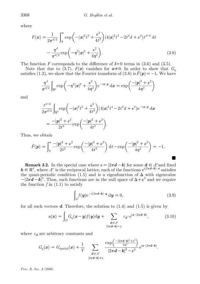
where

FðxÞZ 1

2pd=2

ðNh

exp Kjxj2t2 C k2

4t2

� �ð4jxj2t4K2t2dCk2ÞtdK3 dt

Khd

pd=2exp Kh2jxj2 C k2

4h2

� �: ð3:8Þ

The function F corresponds to the difference of lZ0 terms in (3.6) and (3.5).Note that due to (3.7), F(x) vanishes for xs0. In order to show that Gq

satisfies (1.2), we show that the Fourier transform of (3.8) is FðpÞZK1. We have

hd

pd=2

ðRdexp Kh2jxj2 C k2

4h2

� �eKix$p dx Z exp

Kjpj2Ck2

4h2

� �

and

tdK3

2pd=2

ðRdexp Kjxj2t2C k2

4t2

� �ð4jxj2t4K2t2dCk2ÞeKix$p dx

ZKjpj2Ck2

2t3exp

Kjpj2Ck2

4t2

� �:

Thus, we obtain

FðpÞZðNh

Kjpj2Ck2

2t3exp

Kjpj2 Ck2

4t2

� �dtKexp

Kjpj2Ck2

4h2

� �ZK1:

&

Remark 3.2. In the special case where kZ j2pdKkj for some d 2L�and fixedk 2R

d, where L� is the reciprocal lattice, each of the functions eið2pdKkÞ$x satisfiesthe quasi-periodic condition (1.5) and is a eigenfunction of D with eigenvalueKj2pdKkj2. Thus, such functions are in the null space of DCk2 and we requirethe function f in (1.1) to satisfyð

Df ðyÞeKið2pdKkÞ$y dy Z 0; ð3:9Þ

for all such vectors d. Therefore, the solution to (1.4) and (1.5) is given by

uðxÞZðDGqðxKyÞf ðyÞdyC

Xd2L�

j2pdKkjZk

cd$eix$ð2pdKkÞ; ð3:10Þ

where cd are arbitrary constants and

GqðxÞZGspatialðxÞC1

V

Xd2L�

j2pdKkjsk

exp Kj2pdKkj2Ck2

4h2

� �j2pdKkj2Kk2

eix$ð2pdKkÞ:



Remark 3.3. We note that to derive Gq, it is sufficient to consider the real partof the free-space Green’s function Gfree since the imaginary part of Gfree leads to avanishing sum. Indeed, using the Poisson summation for generalized functions,for kO0, ksj2pdKkj, k 2R

d and x2D, we haveXl2L

ImðGfreeðxC lÞÞeik$l Z p

2Vk

Xd2L�

eix$ð2pdKkÞdðj2pdKkjKkÞZ 0;

where L is a Bravais lattice, L� its reciprocal lattice and V the volume of theprimitive cell. This property may also be seen by replacing the outgoing free-space Green’s function by the incoming one (i.e. its complex conjugate) to obtain(3.2), (3.1) and (3.4). Also, the limiting procedure described in §3a (as analternative to Ewald’s summation) leads to the same conclusion. We were notable to find this fact in the literature except for a particular case in McPhedranet al. (2005).

(a ) A connection with Ewald’s method

Ewald (1921) used an integral representation of the free-space Green’sfunction in dimension dZ3,

1

4p

eikr

rZ

1

2p3=2

ðG

exp Kr2t2 Ck2

4t2

� �dt;

where G is a suitably chosen contour in the complex plane so that the integral iswell defined. Let us consider a different limiting procedure, similar to that in(2.2), to obtain Ewald’s result. Instead of integrating along a contour, we add animaginary part to k, kCil with lOk and consider

Gfreeðr ; lÞZ1

4p

eiðkCilÞr

rZ

1

2p3=2

ðN0exp Kr2t2 C

ðkC ilÞ2

4t2

� �dt ð3:11Þ

with integration over the positive real axis. The expression on the left-hand sideof the formula yields the free-space Green’s function as l/0, whereas theintegral on the right-hand side is well defined only for lOk. However, owing toanalytic dependence on l, it is possible to use the integral in (3.11) to obtain anexpression for the quasi-periodic Green’s function. We proceed with thederivation for dimension dZ3 and note that in dimension dZ2 we may followthe same steps but starting (for lOk) with

i

4H

ð1Þ0 ððkK ilÞrÞZ 1

2p

ðN0exp Kr2t2C

ðkC ilÞ2

4t2

� �dt

t;

instead of (3.11). Similar integrals are available in any dimension d.The fact that the integral in (3.11) is well defined for lOk may be seen using

the primitive

1

2p3=2

ðexp Kr2t2C

ðkC ilÞ2

4t2

� �dt ZK

eðKikClÞr

8prerfc

KikCl

2tCrt

� �

CeðikKlÞr

8prerfc

KikCl

2tKrt

� �



and, using (Abramowitz & Stegun 1970, eqn (7.1.16)) to evaluate the limitsfor lOk,

limt/0C

KeðKikClÞr

8prerfc

KikCl

2tCrt

� �C

eðikKlÞr

8prerfc

KikCl

2tKrt

� �Z 0

and

limt/N

KeðKikClÞr

8prerfc

KikCl

2tCrt

� �C

eðikKlÞr

8prerfc

KikCl

2tKrt

� �Z

1

4p

eðikKlÞr

r:

As a starting point to construct the quasi-periodic Green’s function, we use(3.11) and for lOk consider

Gqðx; lÞZ1

2p3=2

Xl2L

eik$lðh0exp KjxC lj2t2 C ðkC ilÞ2

4t2

� �dt

C1

2p3=2

Xl2L

eik$lðNhexp KjxC lj2t2 C ðkC ilÞ2

4t2

� �dt: ð3:12Þ

As in Ewald (1921), we introduced a real parameter hO0 to split the region ofintegration into two intervals t2(0, h) and t2(h,N).

In the second term in (3.12), we set lZ0 since the integral is convergent for alllR0. Thus, we obtain

GspatialðxÞZ1

2p3=2

Xl2L

eik$lðNh

exp KjxC lj2t2 C k2

4t2

� �dt: ð3:13Þ

We note that explicit integration yields

1

2p3=2

ðNhexp KjxC lj2t2 C k2

4t2

� �dt Z

1

4p

cosðkjxC ljÞjxC lj

�

KeKikjxClj

2jxC lj erfKik

2hC jxC ljh

� �C

eikjxClj

2jxC lj erfKik

2hKjxC ljh

� ��;

an expression that may be found in some numerical procedures for Ewald’smethod. We note that this formula requires appropriate modifications incomputing contributions of the error function to avoid loss of accuracy. Weinstead write

GspatialðxÞZ1

4p3=2

Xl2L

eik$lðNlogð2hÞ

exp KjxC lj2 e2s

4Ck2eK2s Cs

� �ds; ð3:14Þ

where we changed the integration variable from t to s, tZes/2. This expressioncoincides with (3.2) for dZ3.



In the first term in (3.12), we exchange the order of summation and integrationsince lOk. We then use the Poisson summation formula in proposition 2.1to obtain

1

2p3=2

ðh0exp

ðkC ilÞ2

4t2

� �Xl2L

eik$leKjxClj2t 2 dt

Z1

2V

ðh0exp

ðkC ilÞ2

4t2

� � Xd2L�

eix$ð2pdKkÞexp Kj2pdKkj2

4t2

� �dt

t3;

where L� is the reciprocal lattice. By again switching the order of summation andintegration, we arrive at

1

2V

Xd2L�

eix$ð2pdKkÞðh0exp

Kj2pdKkj2 CðkC ilÞ2

4t2

� �dt

t3

Z1

V

Xd2L�

eix$ð2pdKkÞexp Kj2pdKkj2CðkCilÞ24h2

� �j2pdKkj2KðkC ilÞ2

:

Denoting the right-hand side as

GFourierðx; lÞZ1

V

Xd2L�

eix$ð2pdKkÞexp Kj2pdKkj2CðkCilÞ24h2

� �j2pdKkj2KðkC ilÞ2

;

we observe that GFourier(x, l) is an analytic function in l and, thus, may beextended to the region lO0. This leads us to consider the quasi-periodic Green’sfunction defined by the limiting procedure

GqðxÞZGspatialðxÞC liml/0C

GFourierðx; lÞ; ð3:15Þ

valid for any real parameter hO0. To evaluate the limit, we have (e.g. Gel’fand &Shilov 1964, ch. III, §1.3)

liml/0C

1

j2pdKkj2KðkC ilÞ2Z

1

j2pdKkj2Kk2C

ip

2j2pdKkj ðdðj2pdKkjKkÞ

Kdðj2pdKkjCkÞÞ:

For kO0, we arrive at

GFourierðxÞZ liml/0C

GFourierðx; lÞ

Z1

V

Xd2L�

eix$ð2pdKkÞexpKj2pdKkj2Ck2

4h2

� �

!1

j2pdKkj2Kk2C

ip

2kdðj2pdKkjKkÞ

� �: ð3:16Þ

The sum involving the delta function vanishes provided ks 2pdKkj j, whered 2L� and, under this assumption, we obtain (3.1).



4. Fast convolutions with Green’s function

Representation of the quasi-periodic Green’s function as a sum of two rapidlyconvergent series (3.1) and (3.2) yields a fast and accurate algorithm for itsapplication as a convolution. We truncate these series and obtain a separatedrepresentation by approximating the integral in (3.2) via a sum of Gaussians.Using the resulting approximation of Green’s function, we prove an accuracyestimate (in operator norm) for its application. We then present the algorithm toapply the operator, and estimate its computational complexity. We illustrate thealgorithm by presenting several examples.

(a ) Approximation of Green’s function

Let us outline how we obtain an approximation of the quasi-periodic Green’sfunction (3.4).

Owing to the exponential decay of the terms in GFourier, we truncate theFourier sum

~GFourierðxÞZ1

V

Xd2L�

j2pdKkj%kb

exp Kj2pdKkj2Ck2

4h2

� �j2pdKkj2Kk2

eix$ð2pdKkÞ; ð4:1Þ

where we select parameters hO0 and bO0 so that the contribution of thediscarded terms is less than the desired accuracy e.

For Gspatial we perform a similar truncation again using the exponential decayof its terms and, in addition, construct an approximation of Fsing in (3.3) as asum of Gaussians. For a fixed parameter h and given accuracy e, we select aO0to truncate the sum (3.2) as X

l2L

jlj%a

eik$lFsingðxC lÞ;

so that the contribution of the discarded terms is less than e. Then, for fixed k, weapproximate Fsing as in Beylkin et al. (submitted) using a discretization of theintegral. Thus, we obtain an approximation of Fsing as a sum of Gaussians,

SsingðxÞZXNjZ1

qjeKsj jxj2 ; ð4:2Þ

where sjO0 and qjO0. The weights qj depend on the dimension d and theparameter k (see Beylkin et al. (submitted) for details). Using (4.2), weapproximate Gspatial as

~GspatialðxÞZXl2L

jlj%a

eik$lSsingðxC lÞ: ð4:3Þ



Combining (4.1) and (4.3), the quasi-periodic Green’s function is approximated as

~GqðxÞZ ~GspatialðxÞC ~GFourierðxÞ: ð4:4Þ

We note that there are two sources of error in this approximation: (i) a truncationerror due to replacing infinite series by finite sums and (ii) an approximationerror introduced by (4.2). Owing to the exponential decay of the terms inboth series, the number of significant terms depends only logarithmically on thedesired accuracy.

We compute convolutions with ~GFourier in the Fourier domain as

ð~GFourier*f ÞðxÞZ1

V

Xd2L�

j2pdKkj%kb

exp Kj2pdKkj2Ck2

4h2

� �eix$ð2pdKkÞ

j2pdKkj2Kk2f Dð2pdKkÞ; ð4:5Þ

where

f DðpÞZðDf ðxÞeKip$x dx ð4:6Þ

and convolutions with ~Gspatial in the spatial domain as

~Gspatial � f� �

ðxÞZXl2L

jlj%a

eik$lXNjZ1

qj

ðDeKsj jxKyClj2 f ðyÞ dy: ð4:7Þ

We show in dimension dZ2,3 that this approximation of (3.4) by (4.4) yieldsaccurate convolutions in the operator norm.

Proposition 4.1. For any eO0, we may choose the splitting parameter h, theFourier truncation parameter b in (4.1) and the spatial truncation parameter a in(4.3) so that

kðGqK~GqÞ � f kLpðDÞ%ekf kLpðDÞ;

for f 2LpðDÞ, 1%p%N.

We note that the parameters h, b and a are interdependent and their selectionis discussed in §4b.

Proof. Using Minkowski’s inequality for convolutions (e.g. Grafakos 2004,p. 20), we have

kðGqK~GqÞ � f kLpðDÞ%k GqK~Gq

� �kL1ðDÞkf kLpðDÞ

% kGspatialK~GspatialkL1ðDÞCkGFourierK~GFourierkL1ðDÞ

� �kf kLpðDÞ:



We may choose hO0 and bO1 so that

1

V

Xd2L�

j2pdKkjOkb

exp Kj2pdKkj2Ck2

4h2

� �j2pdKkj2Kk2

%e

3V

and, thus, ��GFourierK~GFourier

��L1ðDÞ

%e

3: ð4:8Þ

We now estimate the spatial error by

kGspatialK~GspatialkL1ðDÞ

%

��Xl2L

jlj%a

eik$l FsingðxC lÞKSsingðxC lÞ� �

CXl2L

jljOa

eik$lFsingðxC lÞ��L1ðDÞ

%Xl2L

jlj%a

ðDjFsingðxC lÞKSsingðxC lÞj dxC

ðD

Xl2L

jljOa

FsingðxC lÞdx: ð4:9Þ

Next, we may choose aO0 so that the integrand in the second term satisfiesXl2L

jljOa

FsingðxC lÞ% e

3V;

for x2D and, thus, ðD

Xl2L

jljOa

FsingðxC l Þdx% e

3: ð4:10Þ

In what follows, let us first consider dimension dZ3. To estimate the first termin (4.9), as in Beylkin et al. (submitted), we construct the spatial approximationSsing for accuracy e1O0 and range parameter 0!d%diam(D)/2,

jFsingðrÞKSsingðrÞj%

1

r; for 0%r!d;

e1

r; for rRd:

8>>><>>>:

ð4:11Þ

We use (3.2) and (4.3), where we split the lZ0 term to estimateðDjFsingðxÞK SsingðxÞj dxC

Xl2L

0!jlj%a

ðDjFsingðxC lÞKSsingðxC lÞj dx: ð4:12Þ



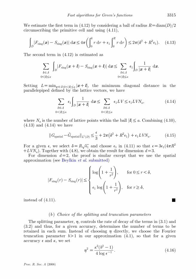
We estimate the first term in (4.12) by considering a ball of radius RZdiam(D)/2circumscribing the primitive cell and using (4.11),ð

DjFsingðxÞKSsingðxÞj dx%4p

ðd0r dr Ce1

ðRdr dr

� �%2pðd2 CR2e1Þ: ð4:13Þ

The second term in (4.12) is estimated as

Xl2L

0!jlj%a

ðDjFsingðxC lÞK SsingðxC lÞj dx%

Xl2L

0!jlj%a

e1

ðD

1

jxC lj dx:

Setting LZminx2D;0!jlj%a jxC lj, the minimum diagonal distance in theparallelepiped defined by the lattice vectors, we have

Xl2L

0!jlj%a

e1

ðD

1

jxC lj dx%Xl2L

0!jlj%a

e1LV%e1LVNa; ð4:14Þ

where Na is the number of lattice points within the ball jlj%a. Combining (4.10),(4.13) and (4.14) we have

kGspatialK ~GspatialkL1ðDÞ%e

3C2p d2CR2e1

� �Ce1LVNa: ð4:15Þ

For a given e, we select dZRffiffiffiffie1

pand choose e1 in (4.11) so that eZ3e1ð4pR2

CLVNaÞ. Together with (4.8), we obtain the result for dimension dZ3.For dimension dZ2, the proof is similar except that we use the spatial

approximation (see Beylkin et al. submitted)

jFsingðrÞKSsingðrÞj%log 1C

1

r2

!; for 0%r!d;

e1 log 1C1

r2

!; for rRd;

8>>>>><>>>>>:

instead of (4.11). &

(b ) Choice of the splitting and truncation parameters

The splitting parameter, h, controls the rate of decay of the terms in (3.1) and(3.2) and thus, for a given accuracy, determines the number of terms to beretained in each sum. Instead of choosing h directly, we choose the Fouriertruncation parameter bO1 in our approximation (4.1), so that for a givenaccuracy e and k, we set

h2 Zk2ðb2K1Þ4 log eK1

: ð4:16Þ



With this selection of h, note that in (3.1) the discarded terms jpjRkb satisfy

exp Kðjpj2Kk2Þ4h2

� �jpj2Kk2

%e

k2ðb2K1Þ :

With h given by (4.16), we now select the spatial truncation parameter a so thatthe contribution of the discarded terms in (3.2) is below the desired accuracy.

Although we only require bO1, in practice the choice of this parameter doesdepend on k and e. For moderate size k we select bw3, for large k we may select asmaller b and for small k we need to choose b larger.

Remark 4.2. Different choices of h have been made in several papers consideringEwald’s summation (e.g. Catti (1978) or Jordan et al. (1986) for kZ0). We wouldlike to point out (see also Moroz 2006; Oroskar et al. 2006 or Beylkin et al.submitted) that some choices of h may induce numerical cancellation resulting in aloss of accuracy. For example, choosing h too small leads to (3.1) and (3.2) to belarge simultaneously and to have opposite signs for jxjw0.

(c ) Algorithm for convolution with the quasi-periodic Green’s function

We describe an algorithm and estimate its complexity for computingvolumetric convolutions with the quasi-periodic Green’s function approximation(4.4). We assume that the input function and its Fourier transform (4.6) aregiven, and we are free to discretize them as needed. In the description of thealgorithm to compute

gðxÞZðD

~GqðxKyÞf ðyÞ dy;

we refer to f and g as the input and the output function, respectively. We want tocompute this convolution for any given accuracy e.

Initialization:

(i) Truncation of the Fourier sum. For a fixed k and a given accuracy e, weselect b that determines h in (4.16).

(ii) Truncation and approximation of the spatial sum. For a fixed k and agiven accuracy e, we construct Ssing as an N-term Gaussian approximation(4.2). We denote by Na the total number of lattice points that satisfyjlj%a. We note that Nwðlog eK1Þ2 (see Beylkin et al. submitted) andNawðlog eK1Þd due to the exponential decay of (3.3).

(iii) Discretization of the input function. We use the multiresolution algorithmin Beylkin et al. (2008) to adaptively discretize the input function using atensor product basis with p scaling functions per dimension. If Nbox is thetotal number of boxes used to represent the input function with accuracye, then the total number of input points is NinZNboxp

d. In practicalapplications, we choose pwlog eK1 since it improves the overallperformance. Thus, we have NinwNboxðlog eK1Þd. We note that it is nothard to construct examples of functions for which an adaptiverepresentation offers no advantage; in such cases, the number of pointsis Ninwkd due to the required Nyquist sampling rate. Thus, in the worst

case, we have NinwkdCC1ðlog eK1Þd.



(iv) Initialization of the output function. The output function, a sum of spatialand Fourier contributions, is evaluated on a user chosen set of Nout points.While the spatial contribution may retain an adaptive structure if we usethe algorithm from Beylkin et al. (2008), the Fourier contribution resultsin O(kd) points due to the required Nyquist sampling rate. Thus, unlessthere are special circumstances, Noutwkd. Again, in the worst case wehave NoutwkdCC2ðlog eK1Þd.

Applying the operator:

(i) Convolution with ~Gspatial. Using the algorithm in Beylkin et al. (2008), the

complexity of applying ~Gspatial in (4.7) is OðNa$p$N$NinÞ. Alternatively, thefast Gauss transform (see Greengard & Strain 1991; Strain 1991;Greengard & Sun 1998) may be used, which results in a similar computa-tional complexity. Although p$N is formally estimated as p$Nwðlog eK1Þ3,we note that within the range of parameters we experimented with, thisproduct behaves effectively as a constant (the overestimation is, in part,due to the fact that the algorithm in Beylkin et al. (2008) does not use allGaussian terms on all scales). Note that in (4.7) the term lZ0 dominatesthe computational cost since this is the only term contributing to fine scalesin a multiresolution representation of the operator. With these caveats, the

computational complexity of computing (4.7) is O kdCC3ðlog eK1Þd� �

,where C3 is a constant.

(ii) Convolution with ~GFourier. We evaluate the Fourier transform of the inputfunction at the reciprocal lattice points within the sphere j2pdKkj%kband denote by NF their total number. We note that NF wðlog eK1Þd due tothe exponential decay of the terms in (3.1). Given a set of locations x toevaluate (4.5), we use the USFFT (Dutt & Rokhlin 1993; Beylkin 1995;Lee & Greengard 2005) to evaluate the trigonometric sum. Thus, thecomputational complexity is OðNoutCNFÞCOðkd log kÞ, or O kd log kC

�C4ðlog eK1ÞdÞ, where C4 is a constant.

We note that the performance of both, the spatial and Fourier, components ofour method has been tested and timed independently in the references mentionedabove. We would like to add that, in some applications, the semi-analytic natureof our approximation may allow for additional savings.

(d ) Examples

We start by comparing values of the quasi-periodic Green’s function computedusing ~Gq in (4.4) and those of its alternative representation in McPhedran et al.(2000). The two-dimensional quasi-periodic Green’s function is written inMcPhedran et al. (2000) as

GLðxÞZi

4H

ð1Þ0 ðkrÞC

Xl2Z

SAl JlðkrÞeKilq

!; ð4:17Þ

where xZðr cos q; r sin qÞ and the coefficients SAl are computed as lattice sums.


−10 −8 −6 −4 −2 0−12

−10

−8

−6

−4

−2

0

(a)

0 0.1 0.2 0.3 0.4 0.5

(b)

Figure 1. Error plots for a two-dimensional quasi-periodic Green’s function with kZð2; 7=10Þ andkZ10 for a hexagonal lattice with lattice vectors l1Zð1; 0Þ and l2Zð1=2;

ffiffiffi3

p=2Þ. (a) The absolute

error jReð~Gqðx1; 0ÞÞKReðGLðx1; 0ÞÞj for x1 2 ð10K10; 1=2Þ using a log–log scale. (b) The absoluteerror jImð~Gqðx1; 0ÞÞKImðGLðx1; 0ÞÞj for x1 2 ð0; 1=2Þ using a log scale on the vertical axis.


We note that the representation in (4.17) allows us only to evaluate Green’sfunction and does not provide an algorithm for its application as an operator. Bycontrast, our approach treats Green’s function as an operator and constructs anapproximation that yields a fast and accurate algorithm for its application. Forthe purpose of comparison, we implemented the evaluation of Green’s function in(4.17) by computing the coefficients SA

l in (4.17) as lattice sums, writingSAl ZDSlCSG

l . We use (McPhedran et al. 2000, eqn (17)) to compute DSl and(Linton 1998, eqns (2.49), (2.53) and (2.54)) to compute SG

l .In figure 1, we display the error between (4.17) and our approximation ~Gq in

(4.4) constructed for accuracy ez10K9. We note that the discrepancy near rZ0is due to our method of approximating Gq and does not affect its application asan operator (beyond accuracy ez10K9) as is demonstrated in proposition 4.1.

Next we verify accuracy of our algorithm by considering the quasi-periodicfunction

uðxÞZffiffiffiffiffiffi2a

p

reKik$x

Xl2L

X3nZ1

eKajxKrnClj2 ð4:18Þ

with parameters aZ300, kZ(1/3, 4/7), r1Z(0, 0), r2Z(1/10, 1/10) and r3Z(K3/20, 1/10), where the sum is over the square lattice generated by the lattice vectorsl1Zð1; 0Þ and l2Zð0; 1Þ. We treat u as a solution of (1.4) and (1.5) and analyticallycompute the corresponding right-hand side in (1.4),

f ðxÞZffiffiffiffiffiffi2a

p

reKik$x

Xl2L

X3nZ1

eKajxKrnClj2

! 4aC jkj2K4a2jxKrn C lj2K4iak$ðxKrn C lÞKk2� �

: ð4:19ÞWe construct an approximate two-dimensional quasi-periodic Green’s function withkZ30, and apply it to f so that we can compare the result with the exact solution u.The parameter a was chosen so that the Fourier transform of the function in (4.19)remains significant well beyond the disc of radius k. Such choice allows us to test


(a) (b)

Figure 3. A quasi-periodic Green’s function with kZ(3, 5) and kZ100 for a two-dimensionalhexagonal lattice with lattice vectors l1Zð1; 0Þ and l2Zð1=2;

ffiffiffi3

p=2Þ plotted in the region

½K1=2; 1=2�!½K1=2; 1=2�: (a) a real part and (b) an imaginary part.

–6

–8

–10

–12

–14

–16–0.6 –0.4 –0.2 0 0.2 0.4 0.6

Figure 2. Absolute error of the difference between the exact and the computed solutions of (1.4)and (1.5) with f in (4.19). The error is plotted along the diagonal of the primitive cell using a logscale on the vertical axis.


both the spatial and Fourier parts of the algorithm. In figure 2, we display theabsolute error plotted along the diagonal of the primitive cell. Green’s function wasapproximated with eZ10K11, whereas the L2-norm of the solution is kuk2z1:76and that of the right-hand side is kf k2z1:31$103. This result agrees with theestimate in proposition 4.1.

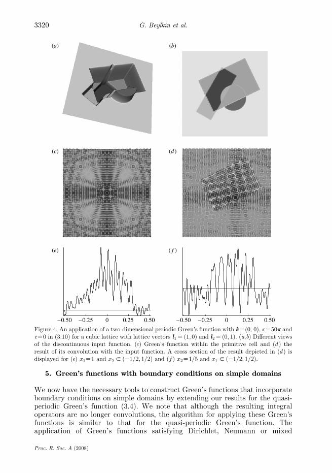
Next, we illustrate the results of convolving with several quasi-periodic Green’sfunctions. In figure 3, we illustrate the application of a two-dimensional quasi-periodic Green’s function to a delta function. The motivation for presenting thisexample is twofold: (i) to demonstrate that our approach is applicable to functionswhose Fourier transforms have slow decay and (ii) to illustrate Green’s functionitself. In figure 4, we display the result of convolving a periodic Green’s functionwitha fairly complicated function with jump discontinuities. We also display crosssections of the (periodic) output function.


(a) (b)

(c) (d )

(e) ( f )

–0.50 –0.25 0 0.25 0.50 –0.50 –0.25 0 0.25 0.50

Figure 4. An application of a two-dimensional periodic Green’s function with kZ(0, 0), kZ50p andcZ0 in (3.10) for a cubic lattice with lattice vectors l1Zð1; 0Þ and l2Zð0; 1Þ. (a,b) Different viewsof the discontinuous input function. (c) Green’s function within the primitive cell and (d ) theresult of its convolution with the input function. A cross section of the result depicted in (d ) isdisplayed for (e) x1Z1 and x2 2 ðK1=2; 1=2Þ and ( f ) x2Z1/5 and x1 2 ðK1=2; 1=2Þ.


5. Green’s functions with boundary conditions on simple domains

We now have the necessary tools to construct Green’s functions that incorporateboundary conditions on simple domains by extending our results for the quasi-periodic Green’s function (3.4). We note that although the resulting integraloperators are no longer convolutions, the algorithm for applying these Green’sfunctions is similar to that for the quasi-periodic Green’s function. Theapplication of Green’s functions satisfying Dirichlet, Neumann or mixed



boundary conditions is again split between the spatial and the Fourier domains.In the spatial domain, we use separated representations involving Gaussians andin the Fourier domain apply a simple combination of multiplication operators.

For ease of notation, we consider the two-dimensional case with Dirichletboundary conditions on the primitive cell DZ ½K1=2; 1=2�!½K1=2; 1=2�. Weconstruct these Green’s functions using the periodic Green’s function (with 2kinstead of k), satisfying

ðDC4k2ÞGpðxÞZKdðxÞand (1.3) with kZ0. We note that the formal description of the periodic Green’sfunction in this case is of the form

G formalp ðx 1; x2ÞZK

1

4

XNn1ZKN

XNn2ZKN

Y0 2k

ffiffiffiffiffiffiffiffiffiffiffiffiffiffiffiffiffiffiffiffiffiffiffiffiffiffiffiffiffiffiffiffiffiffiffiffiffiffiffiffiffiffiffiffiffiffiffiffiffiðx 1Cn1Þ2Cðx 2Cn2Þ2

q� �;

since, in (1.6), the sum associated with the imaginary part of the free-spaceGreen’s function is zero, l1Zð1; 0Þ and l2Zð0; 1Þ.

We write Gp via the sum of two rapidly convergent series in (3.4),

Gpðx 1; x 2ÞZ1

2p

Xn2Z2

ðNlogð2hÞ

exp KjxCnj2 e2s

4C4k2eK2s

� �ds

CXm2Z2

exp Kp2jmj2Ck2

h2

� �4 p2jmj2Kk2� � e2pix$m:

We obtain Green’s function with Dirichlet boundary conditions on D as

GDðx1;x2;y1;y2ÞZGp

x1Ky12

;x2Ky2

2

� �KGp

x 1Cy1C1

2;x 2Ky2

2

� �

KGp

x1Ky12

;x 2Cy2C1

2

� �CGp

x1Cy1C1

2;x2Cy2C1

2

� �:

ð5:1ÞFor xsy, we have DxCk2

� �GDðx; yÞZ0 since each of the four summands in (5.1)

is a Helmholtz Green’s function with parameter 2k. The only singularity is atxZy, in which case the first term in (5.1) yields

Dx Ck2� �

GDðx;yÞZKdðxKyÞ:Since Gp is periodic with period one and is even, the terms in (5.1) cancel eachother on the boundary so that GD satisfies the Dirichlet boundary conditions,GDðG1=2; x 2; y1; y2ÞZ0 and GDðx1;G1=2; y1; y2ÞZ0.

Following the approach in §3, we split (5.1) between the spatial and the

Fourier domains GDZGDspatialCGD

Fourier and then approximate these components.As in §4a, we approximate the spatial part GD

spatial by a sum of Gaussians. For a

desired accuracy e and fixed h, we select aO0 to satisfy (4.10) and construct qjand sj for jZ1,., N in (4.11) to obtain the separated representation

~GDspatialðx1; x2; y1; y2ÞZ

Xffiffiffiffiffiffiffiffiffiffiffin21Cn2

2

p%a

XNjZ1

qjSj;n1ðx1; y1ÞSj;n2

ðx2; y2Þ; ð5:2Þ



where

Sj;nðx; yÞZ exp Ksj

4ðxKyC2nÞ2

� �Kexp K

sj

4ðxCyC1C2nÞ2

� �: ð5:3Þ

Thus, the application of the operator (5.2) separates along each direction and wecompute ð

D

~GDspatialðx; yÞf ðyÞ dy Z

XNjZ1

qjXffiffiffiffiffiffiffiffiffiffiffin21Cn2

2

p%a

ð1=2K1=2

Sj;n2ðx2; y2Þ

!

ð1=2K1=2

Sj;n1ðx1; y1Þf ðy1; y2Þdy1 dy2;

which may be accelerated further using fast algorithms described in §4.In the Fourier domain, for a desired accuracy e and fixed h, we select bO1 to

satisfy (4.8) and obtain

~GDFourierðx1; x2; y1; y2ÞZ

X2p

ffiffiffiffiffiffiffiffiffiffiffiffim2

1Cm2

2

p%kb

expKp2 m2

1Cm22ð ÞCk2

h2

� �4 p2 m2

1 Cm22ð ÞKk2ð Þ e

ipðm1x 1Cm2x 2Þ

! eKipm1y1Keipm1ðy1C1Þ� �

eKipm2y2Keipm2ðy2C1Þ� �

: ð5:4Þ

We apply this operator as

ðD

~GDFourierðx;yÞf ðyÞ dy Z

X2p

ffiffiffiffiffiffiffiffiffiffiffiffim2

1Cm2

2

p%kb

expKp2 m2

1Cm22ð ÞCk2

h2

� �4 p2 m2

1 Cm22ð ÞKk2ð Þ e

ipðm1x 1Cm2x 2Þ

!ðf Dðpm1;pm 2ÞKeipm1f DðKpm1;pm 2Þ

Keipm 2f Dðpm1;Kpm 2ÞCeipðm1Cm 2Þf DðKpm1;Kpm 2ÞÞ;ð5:5Þ

where f D is given in (4.6). We use USFFT to evaluate (5.5) as in §4c.

Remark 5.1. As described by Keller (1953), the method of images in dimensiondZ2 yields Green’s function with prescribed boundary conditions for fourbounded regions: (i) rectangle, (ii) equilateral triangle, (iii) isosceles triangleswith angles p=2;p=4;p=4, and (iv) right triangle with angles p=2;p=3;p=6. As anexample of incorporating the Neumann boundary conditions on D, we have

GNðx1;x2;y1;y2ÞZGp

x1Ky12

;x2Ky2

2

� �CGp

x1Cy1C1

2;x2Ky2

2

� �

CGp

x1Ky12

;x2Cy2C1

2

� �CGp

x1Cy1C1

2;x2Cy2C1

2

� �;

where GNx 2ðG1=2; x2; y1; y2ÞZ0 and GN

x 1ðx1;G1=2; y1; y2ÞZ0, where GN

xi ZvGN=vxi,iZ1, 2.

We note that we can mix Dirichlet and Neumann boundary conditions since itrequires only appropriate sign changes in the previous construction.



Remark 5.2. The construction of Green’s functions with Dirichlet or Neumannboundary conditions on D in dimension dZ3 is completely analogous to the two-dimensional case and is composed of a combination of eight terms. Importantly,their approximations have the same form in all dimensions. For example, in thespatial domain the approximation of Green’s function with Dirichlet boundaryconditions is given by

~GDspatialðx1; x2; x3; y1; y2; y3Þ

Z1

2

Xffiffiffiffiffiffiffiffiffiffiffiffiffiffiffiffiffin21Cn2

2Cn2

3

p%a

XNjZ1

qjSj;n1ðx1; y1ÞSj;n2

ðx2; y2ÞSj;n3ðx3; y3Þ;

where qj are described in (4.2) and Sj,n in (5.3). Similarly, we have an analogueof (5.4),

~GDFourierðx1; x2; x3; y1; y2; y3ÞZ

1

2

X2p

ffiffiffiffiffiffiffiffiffiffiffiffiffiffiffiffiffiffiffim2

1Cm2

2Cm2

3

p%kb

expKp2 m2

1Cm22Cm2

3ð ÞCk2

h2

� �4 p2 m2

1 Cm22 Cm2

3

� �Kk2

� �!eipðm1x 1Cm2x 2Cm3x 3Þ eKipm1y1Keipm1ðy1C1Þ

� �! eKipm2y2Keipm2ðy2C1Þ� �

eKipm3y3Keipm3ðy3C1Þ� �

;

which we apply as a multiplication operator in the Fourier domain. In arbitrarydimension d, we have

~GDspatialðx; yÞZ

1

2dK2

Xjnj%a

XNjZ1

qjYdaZ1

Sj;naðxa; yaÞ;

where Sj;na are given in (5.3) and

~GDFourierðx;yÞZ

1

2dK2

X2pjmj%kb

exp Kp2jmj2Ck2

h2

� �4 p2jmj2Kk2� � eipm$x

YdaZ1

eKipmayaKeipmaðyaC1Þ� �

:

We note that in order to apply Green’s function in higher dimensions, we alsoneed to use a separated representation for the input functions (see Beylkin &Mohlenkamp 2005). Green’s function with Neumann boundary conditions onD has the same form and differs only by changing the sign of appropriate terms.As a result, we may use essentially the same algorithm to apply these operators.To summarize, the results of this section yield fast adaptive solvers for theHelmholtz equation for a variety of boundary conditions.

6. Conclusion and remarks

In this paper, we extend the approach in Beylkin et al. (submitted) for the free-space Helmholtz Green’s function to approximate and apply Green’s functions,which incorporate quasi-periodic Dirichlet or Neumann boundary conditions.The key features of these fast algorithms are: (i) the splitting of application ofoperators between the spatial and the Fourier domains, (ii) the use of separated



representations, and (iii) the ability to achieve a finite, arbitrary accuracy.Algorithms with the last two features have been developed for non-oscillatorykernels and have been used to solve problems in quantum chemistry (seeHarrison et al. 2003, 2004; Yanai et al. 2004a,b). Since these algorithms foroscillatory and non-oscillatory kernels may be considered within the sameframework, we intend to build a unified software framework for their application.We expect further development in this direction. In all cases, we obtainrepresentations of Green’s functions that lead to fast adaptive solvers forcorresponding problems.

Our approach (with minor modifications) is also applicable to the case kZ0.However, using multiresolution, both the interpretation and the application ofthe operator may be kept entirely in the spatial domain and we plan to considerthis case separately.

A natural application of the quasi-periodic Green’s function is in thecomputation of band gaps in crystal structures. We plan to investigate theseapplications with particular attention to potentials (indices of refraction) withsingularities (discontinuities) since, in such cases, the efficiency of our algorithmsdoes not degrade significantly.

We note that our method extends to problems where the lattice dimension isless than the dimension of the embedding space (sometimes referred to asgratings), which will be described elsewhere.

Finally, we note that our results shed new light on Ewald’s approach ofsplitting between spatial and Fourier domains, which we use as a tool to obtainsemi-analytic, separated representations for Green’s functions.

This research was partially supported by NSF grant DMS-0612358, DOE/ORNL grant4000038129, DOE grant DE-FG02-03ER25583 and AFOSR grant FA9550-07-1-0135.

References

Abramowitz, M. & Stegun, I. A. 1970 Handbook of mathematical functions, 9th edn. New York,NY: Dover Publications.

Berry, M. 1981 Quantizing a classically ergodic system: Sinai’s billiard and the KKR method. Ann.Phys. 131, 163–216. (doi:10.1016/0003-4916(81)90189-5)

Beylkin, G. 1995 On the fast Fourier transform of functions with singularities. Appl. Comput.Harmon. Anal. 2, 363–381. (doi:10.1006/acha.1995.1026)

Beylkin, G. & Mohlenkamp, M. J. 2002 Numerical operator calculus in higher dimensions. Proc.Natl Acad. Sci. USA 99, 10 246–10 251. (doi:10.1073/pnas.112329799)

Beylkin, G. & Mohlenkamp, M. J. 2005 Algorithms for numerical analysis in high dimensions.SIAM J. Sci. Comput. 26, 2133–2159. (doi:10.1137/040604959)

Beylkin, G. & Monzon, L. 2005 On approximation of functions by exponential sums. Appl. Comput.Harmon. Anal. 19, 17–48. (doi:10.1016/j.acha.2005.01.003)

Beylkin, G., Cramer, R., Fann, G. & Harrison, R. 2007 Multiresolution separated representationsof singular and weakly singular operators. Appl. Comput. Harmon. Anal. 23, 235–253. (doi:10.1016/j.acha.2007.01.001)

Beylkin, G., Cheruvu, V. & Perez, F. 2008 Fast adaptive algorithms in the non-standard form formultidimensional problems. Appl. Comput. Harmon. Anal. 24, 354–377. (doi:10.1016/j.acha.2007.08.001)

Beylkin, G., Kurcz, C. & Monzon, L. Submitted. Fast convolution with the free space HelmholtzGreen’s function.

Brillouin, L. 1953 Wave propagation in periodic structures. New York, NY: Dover.


http://dx.doi.org/doi:10.1016/0003-4916(81)90189-5

http://dx.doi.org/doi:10.1006/acha.1995.1026

http://dx.doi.org/doi:10.1073/pnas.112329799

http://dx.doi.org/doi:10.1137/040604959

http://dx.doi.org/doi:10.1016/j.acha.2005.01.003






Catti, M. 1978 Electrostatic lattice energy in ionic crystals: optimization of the convergence of

Ewald series. Acta Crystallogr. A 34, 974–979. (doi:10.1107/S0567739478001990)Cruickshank, D., Juretschke, H. & Kato, N. (eds) 1992 P.P. Ewald and his dynamical theory of

X-ray diffraction. Oxford, UK: Oxford University Press.Dienstfrey, A., Hang, F. & Huang, J. 2001 Lattice sums and the two-dimensional, periodic Green’s

function for the Helmholtz equation. Proc. R. Soc. A 457, 67–85. (doi:10.1098/rspa.2000.0656)Dutt, A. & Rokhlin, V. 1993 Fast Fourier transforms for nonequispaced data. SIAM J. Sci.

Comput. 14, 1368–1393. (doi:10.1137/0914081)Ewald, P. 1913 Contributions to the theory of the interferences of X-rays in crystals. Phys. Z 14,

465–472.Ewald, P. 1921 Die berechnung optischer und elektrostatischer gitterpotentiale. Ann. Phys. 64,

253–287. (doi:10.1002/andp.19213690304)Gel’fand, I. M. & Shilov, G. E. 1964 Generalized functions, vol. 1. Properties and operations

(transl. from the Russian by Eugene Saletan). New York, NY: Academic Press.Glasser, M. & Zucker, I. 1980 Lattice sums. In Theoretical chemistry: advances and perspectives

(eds H. Eyring & D. Henderson), pp. 67–139. New York, NY: Academic Press.Grafakos, L. 2004 Classical and modern Fourier analysis. Upper Saddle River, NJ: Pearson

Education, Inc.Greengard, L. & Strain, J. 1991 The fast Gauss transform. SIAM J. Sci. Stat. Comput. 12, 79–94.

(doi:10.1137/0912004)Greengard, L. & Sun, X. 1998 A new version of the fast Gauss transform. In Proc. Int. Congress of

Mathematicians, Berlin, Germany, 18–27 August, vol. III (Extra vol.), pp. 575–584. Bielefeld,Germany: University of Bielefeld.

Ham, F. & Segall, B. 1961 Energy bands in periodic lattice—Green’s function method. Phys. Rev.

124, 1786–1796. (doi:10.1103/PhysRev.124.1786)Harrison, R., Fann, G., Yanai, T. & Beylkin, G. 2003 Multiresolution quantum chemistry in

multiwavelet bases. In Computational science-ICCS 2003, vol. 2660 (eds P. M. A. Sloot,D. Abramson, A. V. Bogdanov, J. Dongarra, A. Y. Zomaya & Y. E. Gorbachev), pp. 103–110.

Lecture Notes in Computer Science. Berlin, Germany: Springer.Harrison, R., Fann, G., Yanai, T., Gan, Z. & Beylkin, G. 2004 Multiresolution quantum chemistry:

basic theory and initial applications. J. Chem. Phys. 121, 11 587–11 598. (doi:10.1063/1.1791051)Joannopoulos, J., Meade, R. & Winn, J. 1995 Photonic crystals: modeling the flow of light.

Princeton, NJ: Princeton University Press.Jordan, K. E., Richter, G. R. & Sheng, P. 1986 An efficient numerical evaluation of the Green’s

function for the Helmholtz operator on periodic structures. J. Comput. Phys. 63, 222–235.

(doi:10.1016/0021-9991(86)90093-8)Keller, J. B. 1953 The scope of the image method. Comm. Pure Appl. Math. 6, 505–512. (doi:10.

1002/cpa.3160060406)Kittel, C. 1986 Introduction to solid state physics, 6th edn. New York, NY: Wiley.Kohn, W. & Rostoker, N. 1954 Solution of the Schrondinger equation in periodic lattices with an

application to metallic lithium. Phys. Rev. 94, 1111–1120. (doi:10.1103/PhysRev.94.1111)Lee, J.-Y. & Greengard, L. 2005 The type 3 nonuniform FFT and its applications. J. Comput.

Phys. 206, 1–5. (doi:10.1016/j.jcp.2004.12.004)Linton, C. M. 1998 The Green’s function for the two-dimensional Helmholtz equation in periodic

domains. J. Eng. Math. 33, 377–402. (doi:10.1023/A:1004377501747)McPhedran, R. C., Nicorovici, N. A., Botten, L. C. & Grubits, K. A. 2000 Lattice sums for gratings

and arrays. J. Math. Phys. 41, 7808–7816. (doi:10.1063/1.1310361)McPhedran, R. C., Nicorovici, N. A. & Botten, L. C. 2005 Neumann series and lattice sums.

J. Math. Phys. 46, 083 509. (doi:10.1063/1.1998827)Moroz, A. 2006 Quasi-periodic Green’s functions of the helmholtz and laplace equations. J. Phys. A

Math. Gen. 39, 11 247–11 282. (doi:10.1088/0305-4470/39/36/009)Oroskar, S., Jackson, D. &Wilton, D. 2006 Efficient computation of the 2D periodic Green’s function

using the Ewald method. J. Comput. Phys. 219, 899–911. (doi:10.1016/j.jcp.2006.06.050)


http://dx.doi.org/doi:10.1107/S0567739478001990

http://dx.doi.org/doi:10.1098/rspa.2000.0656


http://dx.doi.org/doi:10.1002/andp.19213690304


http://dx.doi.org/doi:10.1103/PhysRev.124.1786

http://dx.doi.org/doi:10.1063/1.1791051

http://dx.doi.org/doi:10.1016/0021-9991(86)90093-8

http://dx.doi.org/doi:10.1002/cpa.3160060406

http://dx.doi.org/doi:10.1002/cpa.3160060406

http://dx.doi.org/doi:10.1103/PhysRev.94.1111

http://dx.doi.org/doi:10.1016/j.jcp.2004.12.004

http://dx.doi.org/doi:10.1023/A:1004377501747



http://dx.doi.org/doi:10.1088/0305-4470/39/36/009

http://dx.doi.org/doi:10.1016/j.jcp.2006.06.050


Soukoulis, C. (ed.) 1992 Photonic band gaps and localization. New York, NY: Plenum Press.Strain, J. 1991 The fast Gauss transform with variable scales. SIAM J. Sci. Statist. Comput. 12,

1131–1139. (doi:10.1137/0912059)Yanai, T., Fann, G., Gan, Z., Harrison, R. & Beylkin, G. 2004a Multiresolution quantum

chemistry: analytic derivatives for Hartree–Fock and density functional theory. J. Chem. Phys.121, 2866–2876. (doi:10.1063/1.1768161)

Yanai, T., Fann, G., Gan, Z., Harrison, R. & Beylkin, G. 2004b Multiresolution quantumchemistry: Hartree–Fock exchange. J. Chem. Phys. 121, 6680–6688. (doi:10.1063/1.1790931)

Yasumoto, K. & Yoshitomi, K. 1999 Efficient calculation of lattice sums for free-space periodicGreen’s function. IEEE Trans. Antennas Propagation 47, 1050–1055. (doi:10.1109/8.777130)






fastalgorithmsforhelmholtzgreen’sfunctions · fastalgorithmsforhelmholtzgreen’sfunctions ... of...

Documents