accuracy of cfsr and wfdei precipitation data for brazil: … · accuracy of cfsr and wfdei...
TRANSCRIPT

Accuracy of CFSR and WFDEI PrecipitationData for Brazil: Application in River Discharge
Modelling of the Tocantins Catchment
Jose A.F. Monteiro1,2 Michael Strauch3 Raghavan Srinivasan2
Karim Abbaspour4 Bjorn Gucker1
1Applied Limnology Laboratory, Federal University of Sao Joao del-Rei, MG, BR2Spatial Analysis Laboratory, Texas A&M University, College Station, TX, USA
3Helmholz Centre For Environmental Research (UFZ), Leipzig, Germany4Swiss Federal Institute of Aquatic Science and Technology (Eawag), Dubendorf, Switzerland
SWAT International ConferencePula, Sardinia, Italy
24.06.2015
1

Hydrological Modelling - Input Data Challenges
Input dataI Landscape data
– Topography (DEM)– Soil type– Soil cover (natural vegetation vs. land use)– (River network)
I Weather data– Temperature– Precipitation– (Solar radiation)– (Relative humidity)– (Wind speed)
– Impossible to reassess!
2

Hydrological Modelling - Input Data Challenges
Input dataI Landscape data
– Topography (DEM)– Soil type– Soil cover (natural vegetation vs. land use)– (River network)
I Weather data– Temperature– Precipitation– (Solar radiation)– (Relative humidity)– (Wind speed)– Impossible to reassess!
2

Alternatives to observed weather data
Name Spatial res. Temporal res. Period Reference
CRU 0.5◦ Monthly 1901–2012 Jones et al. (1999)MERRA ∼0.5◦ Hourly 1979–present Rienecker et al. (2011)CFSR ∼0.312◦ Daily 1979–2010 Saha et al. (2010)ERA-Interim 0.75◦ Daily 1979–present Dee et al. (2011)
WFDEI 0.5◦ 3-hourly 1979–2012 Weedon et al. (2014)
CFSR
I First climate reanalysis that includes over the oceans
I More accurate representation of observed mean precipitation intropical regions (Wang et al., 2012)
WFDEI
I WATCH Forcing Data (WFD) methodology applied to ERA-Interim(WFDEI)
I Highest temporal resolution
3

CFSR, WFDEI, INMET and ANA in Brazil
Availability and geographicaldistribution
I INMET observed data– 53* stations: 1980–2010– (15 in the Tocantins
Catchment)
I ANA observed data(precipitation)
– 1974* stations: 1980–2010– (105 in the Tocantins
Catchment)
I CFSR– 7,223 grid cells– (651 in the Tocantins
Catchment)
I WFDEI– 2,822 grid cells– (255 in the Tocantins
Catchment)
* Series with <90% completeness
●●●●
●●●●●
●●
●●●●
●
●●●
●●●
●
●
●
●
●
●●
●●●
●●●
●●●
●● ●●●●
●
●●●
●●
●●●●
●●●●
●●●●●
●●●● ●●
●●
●●
●●●●●
●
●●
●
●
●
●●●●●●
●●●
●
●●
●●●
●
●●
●●●●●●●●●●●
●●
●●
●
●●
●
●
●●
●●
●●●
●●
●●● ●
●●●
●●●●
●●● ●●●●
●
●●●●●
●●
●●
●●
●●●●●
●●
●
●●●●●
●●●
●
●
●●●
●●●
●
●
●
●● ●
●
●● ●●●
●●
●
●●●
●●
●
●
●● ●● ●
● ●●
● ●●●●●
●●
● ●●
●●●
●●●
●●●
●●
●●●●
●
●●
●
●
●●
●●●●
●
●
●●
●
●● ●●●●●●●●● ●
●●●●●
●●
●
●
●●●●
●
●● ●●
●
●●●●●
●● ●
●●●●●
●
●●
●●●●
●
●●
●●●●
●●
●
●●●●
●●●●●●
●●●●
●●
●●●●
●●
●
●
●●
●●
●●
●●
●●●●●
●●
●
● ●
●●●
●●●●●
●●
●● ●
●
●
●●
●
●
●
●●●
●●
●●●●●●
●●●●
●
●
●●●
●
●
●●●
●●
●●
●●
●●
●
●●
●
●●
●
●●● ●
●●
●
●●●
●●●
●●
●
●●
● ●●●
●
●●●
●●●●
●
●●
●
●
●●●●
●●
●●●●
●
●●
●
●
●
●●●●
●
●
●●●
●
●
●
●
●
●●●●
●●●●
●
●●●●
●● ●●
●●●
●
●●●●
●●●
● ●●
● ●●●
●●
●●
●●
●
●
●●
●●●●
●●●
●
●●
●
●●
●●
●●●●
●
●●●
●●●●
●●●●
●
●
●●●
●●●●●
●●
●●●
●
●
●●●
●●● ●
●●
●
● ●
● ●● ●
●
●●●●
●
●● ●●
●
●
●●
●●●
●●●●
●
●
●●●● ●●●●
●●●
●●●
●●●●●
●●●
●●●
●●
●●●●
●●
● ●●●●●
●●
●● ●●●●●
●
●●
●
●●
●●●
●●
●●
● ●
●●●
●● ●
●
● ● ●
●●●
● ●●●●●●
●
●
●
●●
●
● ●●
●●●
●●●
●
●●●
● ● ●●●●
●
●
●●●
●
● ●●●
●●●●●
●
●
●●
●●
●●
●●●
●●●
●●●●
●●
●
●●●●
●●●
● ●
●●●
●●●●●●
●●●●
●●
●● ●
●●●
●●
●
●
●
●●● ●
●●●●
●
●●
●●
● ●●
●●
●●●
●
●●●
●●
●
●●
●
●
●●
●● ●
●●
●●●●
●
●
●●
●●●●
●●
●
●
●
●
●●
●●
●
●●
●●
●●
●●
●●●
●●●
●
●●
●
●●●
● ●
●
●
●●
●●
●●●
●●
●
●
●●
●
●●●
●
● ●●
●●● ●●●
●
●●●
●●
●●●● ●
●
●
●●
●●●
●●●●●
●
●●●
●●
●●●●●
●●●●●●
●
●●
●●●●●●●
●●
●
●
●
●●●●●●
●●
●●
●●
●
●
●●●
●
●
●●
●●●●
●●●
●●●
●
●●●●●●● ●
●●●●
● ●●
●
●●●●
●●●●● ●
●●
● ●●
●●●
●●
●
●
●
●
●●
●●
●
●●
●
●
●●
● ●
●●●●●
●●●●●
●●
●●
●
●●
●●●
●●●
●
●
●●
●●
●●●●●
●●
●
●●●●●●
●●● ●●●●
●●●●●
●●●●●●●●●●●●●●●●●●
●●●●●●●
●
●
●●●●
●●●●●●● ●●●●●
●
● ●●●●●●
●●●●●● ●● ●
●●●
●●●●● ●●● ●
●
●●
●●
●●●
●
●●●●
●●
●●●●●●
●●●●●●●●●●● ●●●●●
●●● ● ●● ●●●
●●●●●●●
● ●
●●●●●●● ●●●
●●
●●●● ●●●
● ●● ●
●●●●
●●●●
●●
●●●●
●●●
●●
●●
●●●●●●● ●●
● ●●●●●●●
●●●
●●●
●●
●●
●●●●●●●●
●●●●●●●
●●● ●●●●●
●
●●●● ●●●●●●●●●●●
●●●●●●
●●●●
●●
●
●●
●●
●● ●●●
●
●●
●● ●●●●●●●●●●●●●
●
●●●
●●●●●
●
●●●●●●●●●
●●
●● ●●●
●●●●●●
●
●
●●●●
●●●●●●●●
●
●●●
●●
●
●
●
●
●
●
●●●
●
●
●●●●●●●●●● ●
●
●●●●●●
●●●
●●●●
●
●●
●●●
●
●
●● ●● ●●●
●●●●●
●●●
●●●
●
●●●●●●●●●●●●
●●
●●
●●
●
●●●●
●
●●●●
●●●
●●●●●
●●
●●
●
●●●●●●●● ●● ● ●●
● ●●●● ●
●●
●
●
●
●
●●
●
●●
●●●●● ●●●●●
●●●●●
●●● ●
●
●●●●●●●●●●●●
●●●
●●●
● ●●●
●●
●●
●
●
●
●●●●
●●●●●●●●● ●●
●●●●●
●●
● ●
●
●●●●
●●●●
●●●● ●●●
●●●●
●●
●●●● ●●●
●●●●●●●●
●●
●●
●●
●
●●●●
●
●
●●●● ●
●
●●●●
●●●
●
●
●
●
●●●
●●●●
●
●●●
●●●●
● ●
●
●●
●
●●●●●● ●
●
●●●●●
●●●●
●●
●●●
●
●●
● ●●●●●● ●●●
●●●●●
●●●
●● ●●
●●
● ●●
● ●●●
●●● ●
●
●●●●
●●
●
●
●●
●●●●●
●●●
●
●●
●
●●
●●
●●●●
●●●●●●
●●
●●
●●
●
●●
●●
●
●●● ●●
●●●●
●
●
●●
● ●
●●●●
●●●●
● ●
●
●●
●
●
●
●●
●●
● ●●●
●●
●●●
●
●
●
●
●
●●
●●
●
●
●●● ●●●●●
●
●●
●●
●●
● ●
●●
●
●●●
●●
●●
●
●●●
●
●
●●
●●●●
● ●
●
●●
●
●
●●● ●
●●
●●●●
●
●
●
●●
●●●●
●●●
●
●●●
●
●●
●●
●
●●●
●
●
●
●
●
●
●
●
●
●
●
●
●
●
●
●
●
●
●
●
●
●
●
●
●
●
●
●
●
●
●
●
●
●
●
●
●
●
●
●
●
●
●
●
●
●
●
●
●
●
●
●
●
−30
−20
−10
0
−70 −60 −50 −40
4

CFSR and WFDEI vs. Observations
Methods
I Analysis restricted to precipitationI Goodness of fit statistics
– Each observation gauge was compared to the nearest CFSR and WFDEIgrid cell
– R2: Coefficient of determination– bR2: Slope × Coeff. of determination (Krause et al., 2005)– NS: Nash-Sutcliffe Efficiency (Nash and Sutcliffe, 1970)– Pbias: Percentage of bias
I Geographical trendsI Comparison of Goodness of fit statistics
– Boxplot– Paired T-test
I Improve further best data set
– CF = ReanalysisObservation
→ ReanalysisCF
= Interpolation– Observation = monthly cumulative precipitation– Observation = monthly averages
5

CFSR and WFDEI vs. Observations
Results
I More general spatial variability in the performance of CFSR
I Worst CFSR performance along the coast and in the South (R2 andbR2)
6
CFSR and WFDEI vs. Observations
Results
●●●●●●●●●●●●●●●●●●●●●●●●●●●●●
●
●●●●●
●●●●●
●●●●●●●●
●●●●●●●●●●●●●●●●●●●●●●●●●●●●●●●●●●●●●●●●
●
●●●
●
●●
●
●
●
●
●●●●●●
●
●
●●
●
●●●●●●●
●
●●●●
●
●●
●
●
●
●
0.00
0.25
0.50
0.75
1.00
Daily Monthly Annual
CFSR
WFDEI
R2
●●●●●●●●●●●●●●●●●●●●●●●●●●●●●●●
●
●
●●
●●●
●
●●●●
●
●●
●
●
●●●●
●
●●●
●
●●
●●●●
●
●
●●●●
●
●●●●
●
●
●●
●●●
●
●●●
●
●
●
●
●
●
●
●
●
●
0.00
0.25
0.50
0.75
1.00
Daily Monthly Annual
bR2
●
●
●
●
●●
●
●
●
●
●
●
●
●
●
●
●
●●●●●●●
●●
●●
●
●
●
●●●●●
●
●
●
●●
●
●●
●●●
●
●
●
●●●
●
●
●●●●●
●●
●
●
●
●
●●
●
●●●
●
●●●●●
●●
●●
●
●
●
●●●●●●●
●
●
●●
●
●
●●●●
●
●
●●●
●
●●●●●
●●
●
●
●
●
●●
●
●●●
●
●●●●●
●●
●●
●
●
●
●●●●●●●
●
●
●●
●
●
●●●●
●
●
●●●
●
●●●●●
●●
●
●
●
●
●
●●●
●●
●
●●
●●●
●●
●●
●
●
●
●●
●
●●
●
●
●
●
●●●
●
●
●
●●●●
●●
●
●
●●●●
●
●●
●
●
●●●●
●
●
●
●
●
●
●
●
●
●●●●●●
●
●●
●
●●●●●●
●
●
●●
●
●●●
●●
●
●●●●
●●
●
●
●
●
●
●
●●●●
●
●●●●●●
●
●
●
●●
●
●
●
●
●●●●●
●●
●
●●
●
●
●
●
●
●●
●
●●
●●●
●●
●
●
●●
●
●
●
●●
●●
●
●
●●●● ●
●●
●
●
●
●
●
●●●●
●
●●
●●
●
●●●●
●
●
●
●
●
●
●
●●●
●●
●
●
●●●●●
●●●●●●●
●
●●●●
●●
●
●
●
●
●
●
●
●●●
●
●●●●●●
●
●●●
●●●●●
●●●●
●
●
●●
●
●
●
●
●
●●
●
●●
●●●
●
●
●●
●
●●
●
●
●●
●●
●
●●
●●●●
●
●
●
●
●
●●●●
●
●●
●●
●
●●●●
●
●
●
●
●
●
●
●●●
●●
●
●
●●●●●
●●●●●●●
●
●●●●
●●
●
●
●
●
●
●
●
●●●
●
●●●●●●
●
●●●
●●●●●
●●●●
●
●
●●
●
●
●
●
●
●●
●
●●
●●●
●
●
●●
●
●●
●
●
●●
●●
●
●●
●
−100
0
100
200
300
Daily Monthly Annual
Pbias●●●●●●●●●●●●●●●●●●●●●●●●●●●●●●●●●●●●●●●●●●●●●●●●●●●●●●●●●●●●●●●●●●●●●●●●
●●●●●●●●●●●●●●●●●●●●●●●●●●●●●●●●●●●● ●●●●●●●●●●●●●●●●●●●●●
●●●●●●●●
●
●●●●●●●●●●●●●●●●
●
●●●●●●●●●●●●●●●●●●●●●●●●●●●●●●●●●●●●●●●●●●●●●●●●●●●●●●●●●●●●●●●●●●●
●●●●●
●●●
●●●●●
●
●●●
●●●●●●
●●
●
●
●
●●●
●
●
●
●
●●
●
●●●●●
●
●
●●
●●
●
●●●●●●
●●
●
●
●
●●
●
●
●
●
●
●●●●●
●●●
●●●
●●
●
●●●
●●●●●
●●
●
●●
●
●
●
●
●
●
●
●
●
●
●
●
●●
●
●
●
●●
●
●
●●
●
●
●
●●●●●●●
●
●●●
●
●
●●●●●●●●●
●
●
●
●
●●
●●●
●●●●●●●●●●●●●●●●●●●●●●●●●●●●●●●●●●●●●●●●●●●●●●●●●●●●●●●●●●●●●●●●●●●●●●●●●●●●●●●●●●●●●●● ●●●●●●●●●●●●●●●●●●●●●●●●●●●●●●●●●●●●●●●●●●●●●●●●●●●●●●●●●●●●●●●●●●●●●●●●●●●●●●●●●●●●●●●●●●●●● ●
●●●●●●●●
●●
●
●●●●●●●●●●●●●●●●●●●
●●
●●●
●●●●●●●●●
●
●●●●●●●●
●
●
●●●●●●●●●●●●●●●●●●●●●●
●●
●
●●●●●●●●●●●●●●●●●●●●●
●
●
●●●●●●●●●●●●●●●●●●●●●●●
●●●●
●
−75
−50
−25
0
Daily Monthly Annual
NS
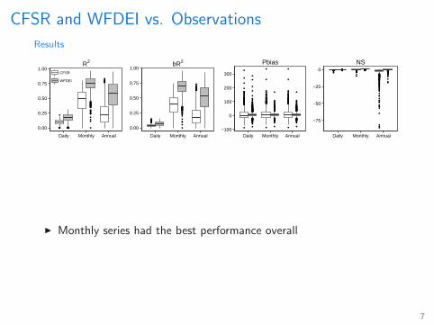
Statistics x CFSR x WFDEI t df p
R2 0.50 0.76 −96.8 2026 p < 0.001bR2 0.39 0.68 −91.5 2026 p < 0.001Pbias 3.4 6.9 −0.031 2026 p = 0.975NS 0.21 0.72 −46.8 2026 p < 0.001
I Monthly series had the best performance overall
I Except for Pbias, all statistics indicated better performance byWFDEI
7

CFSR and WFDEI vs. Observations
Results
●●●●●●●●●●●●●●●●●●●●●●●●●●●●●
●
●●●●●
●●●●●
●●●●●●●●
●●●●●●●●●●●●●●●●●●●●●●●●●●●●●●●●●●●●●●●●
●
●●●
●
●●
●
●
●
●
●●●●●●
●
●
●●
●
●●●●●●●
●
●●●●
●
●●
●
●
●
●
0.00
0.25
0.50
0.75
1.00
Daily Monthly Annual
CFSR
WFDEI
R2
●●●●●●●●●●●●●●●●●●●●●●●●●●●●●●●
●
●
●●
●●●
●
●●●●
●
●●
●
●
●●●●
●
●●●
●
●●
●●●●
●
●
●●●●
●
●●●●
●
●
●●
●●●
●
●●●
●
●
●
●
●
●
●
●
●
●
0.00
0.25
0.50
0.75
1.00
Daily Monthly Annual
bR2
●
●
●
●
●●
●
●
●
●
●
●
●
●
●
●
●
●●●●●●●
●●
●●
●
●
●
●●●●●
●
●
●
●●
●
●●
●●●
●
●
●
●●●
●
●
●●●●●
●●
●
●
●
●
●●
●
●●●
●
●●●●●
●●
●●
●
●
●
●●●●●●●
●
●
●●
●
●
●●●●
●
●
●●●
●
●●●●●
●●
●
●
●
●
●●
●
●●●
●
●●●●●
●●
●●
●
●
●
●●●●●●●
●
●
●●
●
●
●●●●
●
●
●●●
●
●●●●●
●●
●
●
●
●
●
●●●
●●
●
●●
●●●
●●
●●
●
●
●
●●
●
●●
●
●
●
●
●●●
●
●
●
●●●●
●●
●
●
●●●●
●
●●
●
●
●●●●
●
●
●
●
●
●
●
●
●
●●●●●●
●
●●
●
●●●●●●
●
●
●●
●
●●●
●●
●
●●●●
●●
●
●
●
●
●
●
●●●●
●
●●●●●●
●
●
●
●●
●
●
●
●
●●●●●
●●
●
●●
●
●
●
●
●
●●
●
●●
●●●
●●
●
●
●●
●
●
●
●●
●●
●
●
●●●● ●
●●
●
●
●
●
●
●●●●
●
●●
●●
●
●●●●
●
●
●
●
●
●
●
●●●
●●
●
●
●●●●●
●●●●●●●
●
●●●●
●●
●
●
●
●
●
●
●
●●●
●
●●●●●●
●
●●●
●●●●●
●●●●
●
●
●●
●
●
●
●
●
●●
●
●●
●●●
●
●
●●
●
●●
●
●
●●
●●
●
●●
●●●●
●
●
●
●
●
●●●●
●
●●
●●
●
●●●●
●
●
●
●
●
●
●
●●●
●●
●
●
●●●●●
●●●●●●●
●
●●●●
●●
●
●
●
●
●
●
●
●●●
●
●●●●●●
●
●●●
●●●●●
●●●●
●
●
●●
●
●
●
●
●
●●
●
●●
●●●
●
●
●●
●
●●
●
●
●●
●●
●
●●
●
−100
0
100
200
300
Daily Monthly Annual
Pbias●●●●●●●●●●●●●●●●●●●●●●●●●●●●●●●●●●●●●●●●●●●●●●●●●●●●●●●●●●●●●●●●●●●●●●●●
●●●●●●●●●●●●●●●●●●●●●●●●●●●●●●●●●●●● ●●●●●●●●●●●●●●●●●●●●●
●●●●●●●●
●
●●●●●●●●●●●●●●●●
●
●●●●●●●●●●●●●●●●●●●●●●●●●●●●●●●●●●●●●●●●●●●●●●●●●●●●●●●●●●●●●●●●●●●
●●●●●
●●●
●●●●●
●
●●●
●●●●●●
●●
●
●
●
●●●
●
●
●
●
●●
●
●●●●●
●
●
●●
●●
●
●●●●●●
●●
●
●
●
●●
●
●
●
●
●
●●●●●
●●●
●●●
●●
●
●●●
●●●●●
●●
●
●●
●
●
●
●
●
●
●
●
●
●
●
●
●●
●
●
●
●●
●
●
●●
●
●
●
●●●●●●●
●
●●●
●
●
●●●●●●●●●
●
●
●
●
●●
●●●
●●●●●●●●●●●●●●●●●●●●●●●●●●●●●●●●●●●●●●●●●●●●●●●●●●●●●●●●●●●●●●●●●●●●●●●●●●●●●●●●●●●●●●● ●●●●●●●●●●●●●●●●●●●●●●●●●●●●●●●●●●●●●●●●●●●●●●●●●●●●●●●●●●●●●●●●●●●●●●●●●●●●●●●●●●●●●●●●●●●●● ●
●●●●●●●●
●●
●
●●●●●●●●●●●●●●●●●●●
●●
●●●
●●●●●●●●●
●
●●●●●●●●
●
●
●●●●●●●●●●●●●●●●●●●●●●
●●
●
●●●●●●●●●●●●●●●●●●●●●
●
●
●●●●●●●●●●●●●●●●●●●●●●●
●●●●
●
−75
−50
−25
0
Daily Monthly Annual
NS
Statistics x CFSR x WFDEI t df p
R2 0.50 0.76 −96.8 2026 p < 0.001bR2 0.39 0.68 −91.5 2026 p < 0.001Pbias 3.4 6.9 −0.031 2026 p = 0.975NS 0.21 0.72 −46.8 2026 p < 0.001
I Monthly series had the best performance overall
I Except for Pbias, all statistics indicated better performance byWFDEI
7

Interpolating WFDEI
Results
●●●●●●●●●●
●
●
●
●
●
●
●
●
●
●
●
●
0.00
0.25
0.50
0.75
1.00
Daily Monthly Annual
CFSR
WFDEI
WFDEI i.
R2
●
●●●
●
●
●●●●●
●
●●●
●
●
0.00
0.25
0.50
0.75
1.00
Daily Monthly Annual
bR2
●
●
●
●
●
●
●
●
●
●
●
●
●●●
●
●
●
●
●●
●
●
●
●
●
●
●
●
●●
●
●
●
●
●
●●
●
●●
●
●●●●●
●
●
●
●
●
●
●
●
●
●
●
●
●
●
●
●
●
●
●
●
●
●
●
●●
●
●
●
●
●
●
●
●
●
●
−50
0
50
100
Daily Monthly Annual
Pbias●●●●●●● ●
●
●
●
●
●
●
●
●
●●
●●●●●●●●●●● ●●●
●●●●●
●●● ●●●●●
●●
●
●
−50
−40
−30
−20
−10
0
Daily Monthly Annual
NS
Statistics x CFSR x WFDEI t df pCFSR vs. R2 0.58 0.74 −19.6 119 p < 0.001WFDEI bR2 0.50 0.67 −14.6 119 p < 0.001(Tocantins) Pbias 16.3 4.6 5.7 119 p < 0.001
NS 0.37 0.71 −12.5 119 p < 0.001
Statistics x WFDEI x WFDEI i. t df pWFDEI vs. R2 0.74 0.89 −15.3 119 p < 0.001WFDEI i. bR2 0.67 0.88 −15.0 119 p < 0.001(Tocantins) Pbias 4.6 4.0 −0.013 119 p = 0.990
NS 0.71 0.89 −10.4 116 p < 0.001
8

Interpolating WFDEI
Results
0
500
1000
1500
2000
1980 1985 1990 1995 2000 2005 2010Pre
cipi
tatio
n (m
m a
−1)
Observations CFSR WFDEI WFDEI i.
Lowest R2 = 0.36 (ANA 1552001)
0
1000
2000
3000
1980 1985 1990 1995 2000 2005 2010Pre
cipi
tatio
n (m
m a
−1)
Observations CFSR WFDEI WFDEI i.
Lowest bR2 = 0.31 (ANA 1248003)
0
1000
2000
1980 1985 1990 1995 2000 2005 2010Pre
cipi
tatio
n (m
m a
−1)
Observations CFSR WFDEI WFDEI i.
Highest Pbias = 48.0 (ANA 950001)
0
500
1000
1500
2000
2500
1980 1985 1990 1995 2000 2005 2010Pre
cipi
tatio
n (m
m a
−1)
Observations CFSR WFDEI WFDEI i.
Lowest NS = 0.23 (ANA 1146000)
9

Tocantins Catchment SWAT Model
Model set up
Tocantins Catchment
I 803,250 km2
I ∼51% Savannah,∼16% Tropical forest
I Land conversion rateincreasing from Southtowards North
I 10 river gauges3 dams
I SUFI2 with300 simulations
●
●●
●●
●
●
●
●
●1
2
3 4 5
678 9
10 111213
1415
16
171819
2021
2223 24
252627 2829
30
31323334 3536 37
383940
41
42
43444546
4748 49
5051
52
53
54
55
5657 5859
6061 62
63
64 65
666768 69 707172 73
7475 76
7778
7980
81
8283
84
8586
87
88 899091
92939495
9697
9899
100
−15
−10
−5
−55.0 −52.5 −50.0 −47.5
−15
−10
−5
−55.0 −52.5 −50.0 −47.5
Land use
SAVA
FOEB
CRWO
CRDY
Other
10

Tocantins Catchment SWAT Model
Uncalibrated Model Performance
CFSR WFDEI WFDEI interpolated
Gauge Period R2 bR2 NS Pbias R2 bR2 NS Pbias R2 bR2 NS Pbias
Q 2 (16%) Calib. 0.81 0.65 0.36 11.4 0.87 0.58 -0.01 44.4 0.88 0.45 -1.67 104.0Valid. 0.67 0.33 -3.48 110.8 0.83 0.54 -0.20 51.7 0.85 0.40 -2.75 122.1
Q 8 (4%) Calib. 0.73 0.46 -0.78 49.5 0.92 0.78 0.78 11.1 0.90 0.62 0.37 49.2Valid. 0.71 0.36 -2.88 81.1 0.80 0.61 0.24 21.1 0.82 0.53 -0.14 54.5
Q 16 (7%) Calib. 0.69 0.68 0.42 -13.3 0.70 0.52 -0.06 32.7 0.79 0.43 -1.39 97.2Valid. 0.62 0.50 -0.02 28.8 0.55 0.48 0.01 23.4 0.66 0.38 -1.33 95.6
Q 25 (17%) Calib. 0.61 0.52 0.34 -23.4 0.59 0.48 -0.12 24.8 0.69 0.42 -0.95 74.5Valid. 0.61 0.48 -0.22 25.4 0.56 0.44 -0.48 29.5 0.66 0.35 -2.57 99.4
Q 41 (5%) Calib. 0.74 0.74 -0.11 -19.8 0.89 0.75 0.16 -2.8 0.89 0.47 -3.02 67.9Valid. 0.81 0.60 -0.87 16.2 0.79 0.73 0.07 -6.7 0.89 0.45 -4.23 73.1
Q 54 (12%) Calib. 0.88 0.73 0.73 22.8 0.87 0.49 -0.60 83.0 0.84 0.38 -2.78 135.1Valid. 0.47 0.15 -19.61 226.1 0.84 0.38 -4.20 107.5 0.76 0.26 -13.08 198.8
Q 57 (20%) Calib. 0.60 0.49 0.02 -34.9 0.75 0.49 -0.89 40.5 0.73 0.34 -4.40 110.6Valid. 0.71 0.55 -0.31 17.9 0.75 0.43 -2.31 54.9 0.73 0.30 -8.23 130.4
Q 76 (8%) Calib. 0.34 0.20 0.18 -30.9 0.52 0.41 -0.22 54.8 0.57 0.36 -1.06 89.5Valid. 0.71 0.45 -0.60 60.6 0.34 0.29 -0.74 44.4 0.43 0.33 -0.75 55.8
Q 80 (5%) Calib. 0.39 0.17 -0.71 -65.4 0.84 0.60 -0.46 16.9 0.68 0.35 -4.08 84.7Valid. 0.85 0.66 0.22 -37.9 0.94 0.63 -1.23 22.9 0.70 0.33 -7.92 93.1
Q 81 (5%) Calib. 0.80 0.50 -0.56 53.3 0.79 0.54 -0.07 42.0 0.65 0.33 -2.81 108.0Valid. 0.31 0.24 -2.13 39.3 0.30 0.29 -0.63 2.9 0.24 0.24 -0.93 13.5
Weigh. Aver. Calib. 0.66 0.53 0.15 -9.4 0.75 0.53 -0.28 39.3 0.75 0.40 -2.31 96.6Valid. 0.64 0.42 -3.3 63.7 0.68 0.46 -1.22 44.2 0.69 0.34 -4.91 108.7
11

Tocantins Catchment SWAT Model
Model Calibration and Validation
SUFI2 Calibration
Gauge Period p-factor r-factor R2 NS bR2 Pbias
Q 2 (16%) Calib. 0.35 0.35 0.94 0.94 0.91 -3.5Valid. 0.31 0.43 0.93 0.92 0.91 -0.9
Q 8 (4%) Calib. 0.60 0.78 0.88 0.79 0.86 -9.7Valid. 0.72 0.90 0.76 0.61 0.68 -22.0
Q 16 (7%) Calib. 0.36 0.29 0.92 0.92 0.91 -2.1Valid. 0.29 0.27 0.88 0.87 0.77 -9.6
Q 25 (17%) Calib. 0.57 0.46 0.86 0.82 0.70 -16.9Valid. 0.53 0.59 0.83 0.81 0.79 -4.9
Q 41 (5%) Calib. 0.71 2.03 0.85 0.33 0.69 10.4Valid. 0.67 2.18 0.87 0.31 0.73 7.3
Q 54 (12%) Calib. 0.32 0.62 0.84 0.83 0.77 -1.4Valid. 0.29 1.23 0.74 0.43 0.63 16.0
Q 57 (12%) Calib. 0.63 1.14 0.70 0.64 0.59 -15.2Valid. 0.58 1.33 0.64 0.32 0.64 -4.7
Q 76 (12%) Calib. 0.80 1.18 0.60 0.24 0.52 38.4Valid. 0.58 1.12 0.41 0.19 0.38 11.5
Q 80 (12%) Calib. 0.54 1.66 0.58 0.30 0.50 -16.5Valid. 0.47 1.94 0.51 -0.44 0.44 -25.2
Q 81 (5%) Calib. 0.63 1.48 0.53 0.38 0.48 -1.6Valid. 0.52 1.13 0.21 -0.51 0.10 -49.4
Weighed Aver. Calib. 0.52 0.84 0.78 0.70 0.68 -4.5Valid. 0.47 0.99 0.71 0.66 0.47 -4.0
12

Conclusions
I WFDEI and CFSR represent precipitation in Brazilian territoryreasonably well
I WFDEI was significantly more accurate than CFSR
I Interpolation using observation data improved WFDEI further
I Weather reanalysis instead of scarce weather data is a valid optionfor SWAT and allowed for a successful calibration of the TocantinsCatchment
13

Acknowledgements
I Swiss National Science Foundation
I Jaclyn Tech, sending CFSR data
I ANA’s personal, sending flow data
Thank you for your time!
14

References I
Dee, D., S. Uppala, A. Simmons, P. Berrisford, P. Poli, S. Kobayashi, U. Andrae, M. Balmaseda,G. Balsamo, P. Bauer, P. Bechtold, A. Beljaars, L. van de Berg, J. Bidlot, N. Bormann,C. Delsol, R. Dragani, M. Fuentes, A. Geer, L. Haimberger, S. Healy, H. Hersbach, E. Holm,L. Isaksen, P. Kallberg, M. Kohler, M. Matricardi, A. Mcnally, B. Monge-Sanz, J.-J. Morcrette,B.-K. Park, C. Peubey, P. de Rosnay, C. Tavolato, J.-N. Thepaut, and F. Vitart. 2011. TheERA-Interim reanalysis: Configuration and performance of the data assimilation system.Quarterly Journal of the Royal Meteorological Society 137:553–597.
Jones, P. D., M. New, D. E. Parker, S. Martin, and I. G. Rigor. 1999. Surface air temperature andits changes over the past 150 years. Reviews of Geophysics 37:173–199.
Krause, P., D. Boyle, and F. Base. 2005. Comparison of different efficiency criteria for hydrologicalmodel assessment. Advances in Geosciences 5:89–97.
Nash, J., and J. Sutcliffe. 1970. River flow forecasting through conceptual models part I — Adiscussion of principles. Journal of Hydrology 10:282–290.
Rienecker, M., M. Suarez, R. Gelaro, R. Todling, J. Bacmeister, E. Liu, M. Bosilovich, S. Schubert,L. Takacs, G.-K. Kim, S. Bloom, J. Chen, D. Collins, A. Conaty, A. Da Silva, W. Gu, J. Joiner,R. Koster, R. Lucchesi, A. Molod, T. Owens, S. Pawson, P. Pegion, C. Redder, R. Reichle,F. Robertson, A. Ruddick, M. Sienkiewicz, and J. Woollen. 2011. MERRA: NASA’s modern-eraretrospective analysis for research and applications. Journal of Climate 24:3624–3648.
15

References IISaha, S., S. Moorthi, H.-L. Pan, X. Wu, J. Wang, S. Nadiga, P. Tripp, R. Kistler, J. Woollen,
D. Behringer, H. Liu, D. Stokes, R. Grumbine, G. Gayno, J. Wang, Y.-T. Hou, H.-Y. Chuang,H.-M. Juang, J. Sela, M. Iredell, R. Treadon, D. Kleist, P. Van Delst, D. Keyser, J. Derber,M. Ek, J. Meng, H. Wei, R. Yang, S. Lord, H. Van Den Dool, A. Kumar, W. Wang, C. Long,M. Chelliah, Y. Xue, B. Huang, J.-K. Schemm, W. Ebisuzaki, R. Lin, P. Xie, M. Chen, S. Zhou,W. Higgins, C.-Z. Zou, Q. Liu, Y. Chen, Y. Han, L. Cucurull, R. Reynolds, G. Rutledge, andM. Goldberg. 2010. The NCEP climate forecast system reanalysis. Bulletin of the AmericanMeteorological Society 91:1015–1057.
Wang, J., W. Wang, X. Fu, and K.-H. Seo. 2012. Tropical intraseasonal rainfall variability in theCFSR. Climate Dynamics 38:2191–2207.
Weedon, G., G. Balsamo, N. Bellouin, S. Gomes, M. Best, and P. Viterbo. 2014. The WFDEImeteorological forcing data set: WATCH Forcing data methodology applied to ERA-Interimreanalysis data. Water Resources Research 50:7505–7514.
16

Hydrographs
10000
20000
30000
40000
2000 2002 2004 2006 2008 2010Time (months)
Dis
char
ge (
m3 s−1
) Sub−catchment 2
0
1000
2000
3000
2000 2002 2004 2006 2008 2010Time (months)
Dis
char
ge (
m3 s−1
) Sub−catchment 8
5000
10000
15000
20000
25000
2000 2002 2004 2006 2008 2010Time (months)
Dis
char
ge (
m3 s−1
) Sub−catchment 16
5000
10000
15000
20000
2000 2002 2004 2006 2008 2010Time (months)
Dis
char
ge (
m3 s−1
) Sub−catchment 25
10002000300040005000
2000 2002 2004 2006 2008 2010Time (months)
Dis
char
ge (
m3 s−1
) Sub−catchment 41
5000
10000
15000
2000 2002 2004 2006 2008 2010Time (months)
Dis
char
ge (
m3 s−1
) Sub−catchment 54
5000
10000
15000
20000
2000 2002 2004 2006 2008 2010Time (months)
Dis
char
ge (
m3 s−1
) Sub−catchment 57
10002000300040005000
2000 2002 2004 2006 2008 2010Time (months)
Dis
char
ge (
m3 s−1
) Sub−catchment 76
10002000300040005000
2000 2002 2004 2006 2008 2010Time (months)
Dis
char
ge (
m3 s−1
) Sub−catchment 80
1000
2000
3000
4000
2000 2002 2004 2006 2008 2010Time (months)
Dis
char
ge (
m3 s−1
) Sub−catchment 81
17