active learning for multi-objective optimizationactive learning for multi-objective optimization...
TRANSCRIPT
Active Learning for Multi-Objective Optimization
Marcela Zuluaga [email protected] Zurich, Clausiusstrasse 59, 8092 Zurich, Switzerland
Andreas Krause [email protected] Zurich, Universitatstrasse 6, 8092 Zurich, Switzerland
Guillaume Sergent [email protected] de Lyon, 46 Allee d’Italie, 69007 Lyon, France
Markus Puschel [email protected] Zurich, Clausiusstrasse 59, 8092 Zurich, Switzerland
AbstractIn many fields one encounters the challenge ofidentifying, out of a pool of possible designs,those that simultaneously optimize multipleobjectives. This means that usually thereis not one optimal design but an entire setof Pareto-optimal ones with optimal trade-offs in the objectives. In many applications,evaluating one design is expensive; thus, anexhaustive search for the Pareto-optimal setis unfeasible. To address this challenge, wepropose the Pareto Active Learning (PAL)algorithm which intelligently samples the de-sign space to predict the Pareto-optimal set.Key features of PAL include (1) modelingthe objectives as samples from a Gaussianprocess distribution to capture structure andaccomodate noisy evaluation; (2) a methodto carefully choose the next design to evalu-ate to maximize progress; and (3) the abil-ity to control prediction accuracy and sam-pling cost. We provide theoretical bounds onPAL’s sampling cost required to achieve a de-sired accuracy. Further, we show an exper-imental evaluation on three real-world datasets. The results show PAL’s effectiveness;in particular it improves significantly over astate-of-the-art multi-objective optimizationmethod, saving in many cases about 33%evaluations to achieve the same accuracy.
Proceedings of the 30 th International Conference on Ma-chine Learning, Atlanta, Georgia, USA, 2013. JMLR:W&CP volume 28. Copyright 2013 by the author(s).
1. IntroductionA fundamental challenge in many problems in engi-neering and other domains is to find the right balanceamongst several objectives. As a concrete example, inhardware design, one often has to choose between dif-ferent candidate designs that trade multiple objectivessuch as energy consumption, throughput, or chip area.Usually there is not a single design that excels in allobjectives, and therefore one is interested in identify-ing all (Pareto-)optimal designs. Furthermore, oftenin these domains, evaluating the objective functions isexpensive and noisy. In hardware design, for example,synthesis of only one design can take hours or evendays. The fundamental problem addressed in this pa-per is how to predict the Pareto-optimal set at lowcost, i.e., by evaluating as few designs as possible.In this paper we propose a solution that we call thePareto Active Learning (PAL) algorithm. PAL hasseveral key features. It captures domain knowledgeabout the regularity in the design space by using Gaus-sian process (GP) models to predict objective valuesfor designs that have not been evaluated yet. Fur-ther, it uses the predictive uncertainty associated withthese nonparametric models in order to guide the iter-ative sampling. Specifically, PAL’s sampling strategyaims to maximize progress on designs that are likely tobe Pareto-optimal. A set of classification rules iden-tifies designs that are Pareto-optimal and not Pareto-optimal with high probabilty; PAL terminates whenall designs are classified. Finally, PAL is parameter-ized to enable an intuitive, user-controlled tradeoff be-tween sampling cost and prediction accuracy.A main contribution of this paper is the theoreticalperformance analysis of PAL that provides bounds onthe sampling cost required to achieve a desired accu-

Active Learning for Multi-Objective Optimization
racy. These bounds involve the use and quantificationof the so-called hypervolume error, a metric that iscommonly used in multiobjective optimization.Finally, we carry out an extensive empirical evaluation,where we demonstrate PAL’s effectiveness on sev-eral real-world multiobjective optimization problems.Two of these problems (Zuluaga et al., 2012b; Almeret al., 2011) are from different applications in the do-main of hardware design, in which it is very expen-sive to run low level synthesis to obtain the exact costand performance of a single design. The third prob-lem is from software optimization (Siegmund et al.,2012) where different compilation settings are evalu-ated for performance and memory footprint size. Wecompare the performance of PAL against a state-of-the-art multi-objective optimization method calledParEGO (Knowles, 2006). Across all data sets and al-most all desired accuracies PAL outperforms ParEGO,requiring usually about 33% less evaluations.
1.1. Related WorkWe now discuss different lines of related work.Evolutionary algorithms. One class of approachesuses evolutionary algorithms to approximate thePareto frontier using a population of evaluated de-signs that is iteratively evolved (Kunzli et al., 2005;Coello et al., 2006; Zitzler et al., 2002). Most ofthese approaches do not use models for the objectives,and consequently cannot make predictions about un-evaluated designs. As a consequence, a large num-ber of evaluations is typically needed for convergencewith reasonable accuracy. To overcome this challenge,model-based (or “response surface”) approaches ap-proximate the objectives by models, which are fastto evaluate. The best among these appears to beParEGO (Knowles, 2006), which also uses GP modelsof the objective functions. We will compare againstthis approach.Scalarization to the single-obective setting. Analternative approach to multi-objective optimizationproblems is the reduction to a single-objective prob-lem (for which a wealth of methods are available).This is commonly done via scalarization, for exampleby considering convex combinations of the objectivefunctions (Boyd & Vandenberghe, 2004). As a con-crete example, Zhang et al. (2010) proposes a multi-objective evolutionary algorithm framework that de-composes the optimization problem into several single-objective subproblems. A predictive model based onGaussian processes is built for every subproblem, andsample candidates are selected based on their expectedimprovement. A major disadvantage of the scalar-ization approach is that without further assumptions(e.g., convexity) on the objectives, not all Pareto-
optimal solutions can be recovered (Boyd & Vanden-berghe, 2004). Therefore, we avoid scalarization in ourapproach.Heuristics-based methods. Instead of weightedcombinations, numerous domain-specific heuristicshave been proposed that aim at identifying Pareto-optimal solutions. These approaches typically combinesearch algorithms to suit the nature of the problem (D.et al., 2008; Palermo et al., 2009; Zuluaga et al., 2012a)and defy theoretical analysis to provide bounds on thesampling cost. With this work we aim at creating amethod that generalizes across a large range of appli-cations and target scenarios and that is analyzable,i.e., comes with theoretical guarantees.Single-objective active learning and Bayesianoptimization. In the single-objective setting, therehas been much work on active learning, in particularclassification (see, e.g., Settles (2010) for an overview).For optimization, model-based approaches are used toaddress settings where the objective is noisy and ex-pensive to evaluate. In particular in Bayesian opti-mization (see Brochu et al. (2010)), the objective ismodeled as a sample from a stochastic process (oftena Gaussian process). The advantage of this approachis the flexibility in encoding prior assumptions (e.g.,via choice of the kernel and likelihood functions), aswell as the ability to guide sampling: several different(usually greedy) heuristic criteria have been proposedto pick the next sample based on the predictive uncer-tainty of the Bayesian model. A common example isthe EGO approach of Jones et al. (1998), which usesthe expected improvement. Recently, Srinivas et al.(2010) analyzed the GP-UCB criterion, and provedglobal convergence guarantees and rates for Bayesianoptimization. We build on their results to establishguarantees about our PAL algorithm in the multi-objective setting.
1.2. Main ContributionsIn summary, our main contributions include:• the PAL algorithm, which efficiently (i.e., with few
evaluations) identifies the set of Pareto-optimal de-signs in a multi-objective scenario with expensiveevaluations, and which allows user control of accu-racy and sampling cost;• the analysis of PAL that provides theoretical
bounds on the algorithm’s sampling cost to achievea desired target accuracy;• an experimental evaluation to demonstrate PAL’s
effectiveness on three real-world multi-objectiveoptimization problems.

Active Learning for Multi-Objective Optimization
Pareto frontier
df(P )V (P )
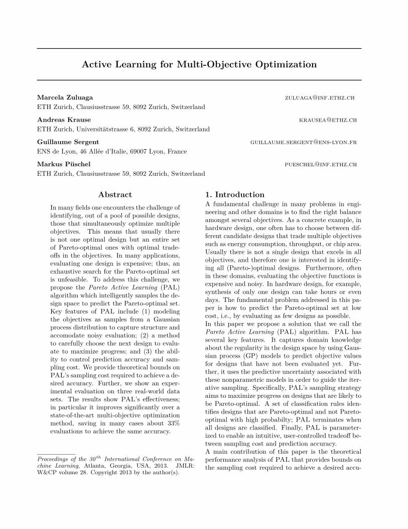
Figure 1. Example of a Pareto frontier in the objectivespace for n = 2 objectives.
2. Background and Problem StatementWe consider a multi-objective optimization problemover a finite1 subset E (called the design space) of Rdfor some d ∈ N. This means we wish to simultaneouslyoptimize n objective functions f1, . . . , fn : E 7→ R. Weuse the notation f(x) = (f1(x), . . . , fn(x)) to refer tothe vector of all objectives evaluated on the input x.The objective space is the image f(E) ⊂ Rn.2Pareto-optimality. The goal in multi-objective op-timization is to identify the Pareto frontier of f . For-mally, we consider the canonical partial order in Rn:y � y′ iff yi ≤ y′i, 1 ≤ i ≤ n, and define the inducedorder on E: x � x′ iff f(x) � f(x′). The set P ⊆ Eof maximal (or Pareto-optimal) points in this order de-termines the Pareto frontier f(P ). Figure 1 visualizesthese concepts for n = 2 objectives.The interest of finding Pareto-optimal points in thedesign space is clear: they represent the best compro-mises amongst the chosen objectives and are the onlydesigns that need to be considered in an application.Problem statement. In many applications, evaluat-ing the objectives f1, . . . , fn is expensive. Therefore,we wish to identify the Pareto-optimal set P ⊂ E with-out evaluating all inputs x ∈ E. Our goal is to developan active learning algorithm that iteratively and adap-tively selects a sequence of designs x1,x2, . . . to beevaluated and that uses this evaluation to classify alldesigns as Pareto optimal or not. The algorithm ter-minates when all designs are classified and returns aprediction P of the Pareto-optimal set P .Prediction quality. A fundamental difference be-tween single- and multi-objective optimization is thatfor the latter it is not obvious which metric to use toevaluate the prediction quality. A very natural pro-posed solution uses the so-called hypervolume (Zitzleret al., 2007), to compute the volumes enclosed by theactual Pareto frontier f(P ) and its prediction f(P ).Formally, we first assume that all the fi are non-
1While our results can be generalized, we focus on thefinite setting to simplify exposition.
2Scalars and functions that evaluate on scalars are writ-ten unbolded; vectors and tuples of functions are boldfaced.
negative (a property that can be established by suit-able shifting if the minimum is known). The hyper-volume V (P ) of a Pareto-optimal set P ⊂ E is thevolume of the area
⋃p∈P {y ∈ Rn : 0 � y � f(p)} en-
closed between the origin and f(P ). In Fig. 1 this areais shaded gray. The hypervolume of an arbitrary setS ⊂ E is defined similarly after all dominated pointsin S have been removed. The quality of a predictionP is then given by the hypervolume error
η = V (P )− V (P ), (1)
which is always positive. The trivial prediction P = Ehas error 0; thus, an important feature of a reasonablealgorithm is that P contains few dominated points.It is clear that prediction is only possible under certainassumptions about f , which are introduced next.Gaussian processes. We model f as a sample froman n-variate Gaussian process (GP) distribution. AGP distribution over a univariate real function f(x)is fully specified by its mean function µ(x) and itscovariance function k(x,x′) (Rasmussen & Williams,2006). The kernel or covariance function k capturesregularity in the form of the correlation of the marginaldistributions f(x) and f(x′).In our multi-objective setting, we model each objectivefunction fi(x) as a sample from an independent3 GPdistribution.On every iteration t in our algorithm we choose adesign xt to evaluate, which yields a noisy sampleyt,i = fi(xt) + νt,i; after T iterations we have a vec-tor yT,i = (y1,i, . . . , yT,i). Assuming νt,i ∼ N(0, σ2)(i.i.d. Gaussian noise), the posterior distribution of fiis a Gaussian process with mean µT,i(x), covariancekT,i(x,x′), and variance σ2
T,i(x):
µT,i(x) = kT,i(x)T (KT,i + σ2I)−1yT,i, (2)kT,i(x,x′) = ki(x,x′)
− kT,i(x)T (KT,i + σ2I)−1kT,i(x′), (3)σ2T,i(x) = kT,i(x,x), (4)
where x,x′ ∈ E, kT,i(x) = (ki(x,xt))1≤t≤T andKT,i = (ki(xj ,x`))1≤j,`≤T . Note that this posteriordistribution captures our uncertainty about f(x) forpoints x ∈ E that have not been evaluated yet. Wenow design an active learning algorithm informed bythis uncertainty.
3. PAL AlgorithmIn this section we describe our algorithm: ParetoActive Learning (PAL). Our approach to predictingPareto-optimal points in E is to train GP models (see
3Note that dependence among the outputs could be cap-tured as well; e.g., (Bonilla et al., 2008).

Active Learning for Multi-Objective Optimization
above) with a small subset of E. The models predictthe objective functions fi, 1 ≤ i ≤ n, allowing us toidentify points in E that are Pareto-optimal with highprobability. A point x, that has not been sampled, ispredicted as f(x) = µ(x) = (µi(x))16i6n. Addition-ally σ(x) = (σi(x))16i6n is interpreted as the uncer-tainty of this prediction. We capture this uncertaintythrough the hyperrectangle4
Qµ,σ,β(x)={y :µ(x)−β1/2σ(x)�y�µ(x)+β1/2σ(x)},(5)
where β is a scaling parameter to be chosen later.We use this uncertainty information to guide our sam-pling and to make a probabilistic assumption on theoptimality of every point x. Since we are only inter-ested in Pareto-optimal points, our algorithm aims atsampling the design space E such that the predictionsgenerated for f(x) are more accurate for points x thatare likely to be Pareto-optimal.At every iteration t, the algorithm uses the predictionsµt(x) and the uncertainties σt(x) to classify a pointx as Pareto-optimal, or not Pareto-optimal. However,some points may remain unclassified. Then, the nextsample to evaluate in the design space is chosen tofurther reduce the number of unclassified points. Thetraining process is terminated when all points are clas-sified; the points classified as Pareto-optimal are thenreturned as the prediction P for P .The pseudocode in Algorithm 1 outlines our approach.After intialization we iterate until a stopping criterionis met; every iteration t consists of three stages: mod-eling, classification, and sampling. These are discussednext including the stopping criterion.Modeling. We use Gaussian process inference to pre-dict the mean vector µt(x) and the standard deviationvector σt(x) of any x ∈ E considering the former eval-uations. Each point x ∈ E is then assigned its uncer-tainty region, which is the hyperrectangle
Rt(x) = Rt−1(x) ∩Qµt,σt,βt+1(x), (6)where βt+1 is a positive value that defines how largethis region is in proportion to σt. Hereby R−1(x) =Rn. In Section 4 we will suggest a value for this pa-rameter. The iterative intersection ensures that alluncertainty regions are non-increasing with t.Within Rt(x), the pessimistic and optimistic outcomesare min(Rt(x)) and max(Rt(x)), respectively, bothtaken in the partial order � and unique.Classification. Our algorithm maintains three setsthat partitions E: in iteration t, Pt is the set of pointsthat are predicted to be Pareto-optimal, Nt the setof points that are predicted to be not Pareto-optimal,and Ut the set of yet unclassified points. In each iter-ation t, each x is assigned to exactly one of the these
4Pessimistically bounding the ellipsoid with radii σi.
Algorithm 1 The PAL algorithm.Input: design space E; GP prior µ0,i, σ0, ki for all 1 ≤ i ≤
n; ε; βt for t ∈ NOutput: predicted-Pareto set P1: P0 = ∅, N0 = ∅, U0 = E {classification sets}2: S0 = ∅ {evaluated set}3: R0(x) = Rn for all x ∈ E4: t = 05: repeat6: Modeling7: Obtain µt(x) and σt(x) for all x ∈ E
{µt(x) = y(x) and σt(x) = 0 for all x ∈ St}8: Rt(x) = Rt−1(x) ∩Qµt,σt,βt+1 (x) for all x ∈ E9: Classification
10: Pt = Pt−1, Nt = Nt−1, Ut = Ut−111: for all x ∈ Ut do12: if there is no x′ 6= x such that min(Rt(x)) + ε �
max(Rt(x′))− ε then13: Pt = Pt ∪ {x}, Ut = Ut \ {x}14: else if there exists x′ 6= x such that
max(Rt(x))− ε � max(Rt(x′)) + ε then15: Nt = Nt ∪ {x}, Ut = Ut \ {x}16: end if17: end for18: Sampling19: Find wt(x) for all x ∈ (Ut ∪ Pt) \ St20: Choose xt+1 = arg maxx∈(Ut∪Pt)\St{wt(x)}21: t = t+ 122: Sample yt(xt) = f(xt) + νt23: until Ut = ∅24: P = Pt
classes. Our algorithm is monotonic in that Pt andNt are non-decreasing sets with respect to t. In otherwords, as soon as a point x is classified as Pareto-optimal (or not Pareto-optimal), it remains classifiedas such. Further, our classification is relaxed by a pa-rameter ε, which informally means inequalities are con-sidered “up to a small error ε”, where ε = (ε, . . . , ε). εis an input to the algorithm.At iteration t, the points in Pt−1 and Nt−1 keep theirclassification. The only points x to be reclassified arethose in Ut−1, done as follows:• If the pessimistic outcome min(Rt(x)) of x is not
dominated by the optimistic outcome max(Rt(x′))of any other point (up to a shift of ε by both),
min(Rt(x)) + ε � max(Rt(x′))− ε,
then x is classified as Pareto-optimal.• If the optimistic outcome max(Rt(x)) of x is dom-
inated by the pessimistic outcome min(Rt(x′)) ofany x′ (up to a shift of ε by both),
max(Rt(x))− ε � min(Rt(x′)) + ε,
then x is classified as non-Pareto-optimal.• All other points remain unclassified.

Active Learning for Multi-Objective Optimization
Intuitively, the parameter ε speeds up classification atthe cost of accuracy, since it makes the requirementsless strict. Figure 2 shows for n = 2 and ε = 0 anexample of a classification at some iteration t.Sampling. After the classification is done, a newpoint xt is selected for sampling with the followingselection rule. Each point x ∈ E is assigned a value
wt(x) = maxy,y′∈Rt(x)
||y − y′||2,
which is the length of the diagonal of its uncertaintyregion Rt(x). Among the points x ∈ Pt ∪ Ut, the onewith the largest wt(x) is chosen as the next sample xtto be evaluated. We refer to wt(xt) as wt.Intuitively, this rule biases the sampling towards ex-ploring, and thus improving the model for, the pointsmost likely to be Pareto-optimal.
f1(x)
f2(x)
d(max(Rt(x)) + ✏
d(min(Rt(x)) + ✏
dwT + 2
p2✏
d
dRt(x) of a point classified as Pareto-optimalRt(x) of a point classified as not-Pareto optimalRt(x) of an unclassified pointSampled points classified as not-Pareto optimalNext sample
Figure 2. Classification and sampling example for n = 2and ε = 0.
Stopping criteria. The training process stops after,say, T iterations when all points in E are classified,i.e., when UT = ∅. The prediction returned is P = PT .The selection of the parameter ε used in the classifica-tion rule impacts both the accuracy and the samplingcost T of the algorithm.
4. Theoretical AnalysisIn this section we analyze the sample complexity ofPAL. Of key importance in the convergence analysisis the effect of the regularity imposed by the kernelfunction k. In our analysis, this effect is quantifiedby the maximum information gain associated with theGP prior. Formally, we consider the information gain
I(y1 . . .yT ;f) = H(f)−H(f | y1 . . .yT ),
i.e, the reduction of uncertainty on f caused by (noisy)observations of f on the T first sampled points. Thecrucial quantity governing the convergence rate is
γT = maxy1...yT
I(y1 . . .yT ;f),
i.e., the maximal reduction of uncertainty achievableby sampling T points. Intuitively, if the kernel k im-
poses strong regularity (smoothness) on f , few sam-ples suffice to gather much information about f , and asa consequence γT grows sublinearly (exhibits a strongdiminishing returns effect). In contrast, if k imposeslittle regularity (e.g., is close to diagonal), γT growsalmost linearly with T . Srinivas et al. (2010; 2012)established γT as key quantity in bounding the regretin single-objective GP optimization. Here, we showthat this quantity more broadly governs convergencein the much more general problem of predicting thePareto-optimal set in multi-criterion optimization.The following theorem is our main theoretical result.Theorem 1. Let δ ∈ (0, 1). Running PAL withβt = 2 log(n|E|π2t2/(6δ)), the following holds withprobability 1− δ.To achieve a maximum hypervolume error of η, it issufficient to choose
ε = η(n− 1)!2nan−1 , (7)
where a = maxx∈E,1≤i≤n{√β1ki(x,x)}.
In this case, the algorithm terminates after at most Titerations, where T is the smallest number satisfying√
T
C1βT γT≥ nan−1
η(n− 1)! . (8)
Here, C1 = 8/ log(1 − σ−2), and γT depends on thetype of kernel used.This means that by specifying δ and a target hypervol-ume error η, PAL can be configured through the pa-rameter ε to stop when the target error is achieved withconfidence 1−δ. Additionally, the theorem bounds thenumber of iterations T required to obtain this result.Later, in Corollary 2, we will specialize the theorem tothe case of a squared exponential kernel.Our strategy for the proof consists of three parts. InSection 4.1, we first analyze how wt decreases with t.We then relate ε and wt to ensure the classification ofall points and thus the termination of the algorithm.In Section 4.2, we relate wt to the hypervolume errorin the predicted Pareto frontier.Finally, in Section 4.3 we analyze the scenario in whichPAL is run with the squared exponential kernel.
4.1. Reduction in UncertaintyThe first step of the proof is to show that with proba-bility at least 1− δ, f(x) falls for all x ∈ E within theuncertainty region (see (5) and (6)):
Rt(x) = Qµ0,σ0,β1(x) ∩ · · · ∩Qµt,σt,βt+1(x),
which is achieved by choosing βt =2 log(n|E|π2t2/(6δ)).

Active Learning for Multi-Objective Optimization
f1(x)
f2(x)d
V (Po)V (Pp)d
dmax(RT (x))
min(RT (x))
dmax(RT (x))
min(RT (x))
Figure 3. Example situation after termation.
Srinivas et al. (2010) showed that information gain canbe expressed in terms of the predicted variances. Sim-ilarly, we show how the cumulative
∑tk=1 wk can also
be expressed in terms of maximum information gainγt. Since the sampling and classification rules used byPAL guarantee that wt decreases with t, we get thefollowing bound for wt. With probability ≥ 1− δ,
wt ≤√C1βtγtt
for all t ≥ 1, (9)
where C1 = 8/ log(1− σ−2) and βt is as before.This means that, with high probability, wt is boundedby O∗(
√γt/t), where O∗ is a variant of the O nota-
tion that hides log factors. The proof is supported byLemmas 3 to 7 found in the supplementary material ofthis paper. Key challenges and differences in compar-ison to Srinivas et al. (2010) include (1) dealing withmultiple objectives; (2) the use of a different samplingcriterion; and (3) incorporating the monotonic classi-fication scheme.We also show that, with probability 1 − δ, all pointswill be classified at iteration T if
wT2 ≤ ε. (10)
This is proved in Lemma 11 found in the supplemen-tary material of this paper.
4.2. Reduction in Hypervolume ErrorWe derive a bound on the hypervolume error (1) thatis achieved once all points have been classified after Titerations and P is returned. As example see Fig. 3,where P has five elements, one of which has been eval-uated (uncertainty due to noise is not shown). Withprobability 1− δ, the points in f(P ) lie inside the un-certainty regions RT (x), x ∈ P . Hence, in this caseη = V (P )− V (P ) ≤ V (Po)− V (Pp), where Po, Pp arethe sets of the optimistic (max(RT (x)) and pessimistic(min(RT (x)) outcomes, respectively, of the points inP . The difference is colored gray in Fig. 3.Using wT , the length of the largest diagonal of anyRT (x), x ∈ P , η is bounded by
η ≤ nan−1wT(n− 1)! , (11)
where a is defined as in Theorem 1. The proof is pre-sented in Lemma 12, which is found in the supplemen-tary material of this paper. Combining (11) with (10)and (9) yields the results from Theorem 1.
4.3. Explicit Bounds for the SquaredExponential Kernel
Theorem 1 holds for general GP models for f(x), withprior µ and covariance function k(x,x′). Srinivas et al.(2010) derived bounds for γT depending on the choiceof kernel for the GP. These can be used to specializeTheorem 1.We illustrate this using the squared exponential ker-nel as example, i.e., k(x,x′) = exp
(l−2‖x− x′‖2
2)
forsome l > 0. From (Srinivas et al., 2010), for n = 1,there exists a constant K such that
γt ≤ K logd+1 t for all t > 1.
For n > 1, since we assume i.i.d. GPs, we thus get
γt ≤ Kn logd+1 t
and hence the following corollary to Theorem 1.Corollary 2. Let ki for all 1 ≤ i ≤ n be the squaredexponential kernels used by PAL. When choosing δ ∈(0, 1), a target hypervolume error η, and an ε that sat-isfies (7), the following holds with probability 1 − δ.PAL terminates after at most T iterations, where Tis the smallest number satisfying√
T log(1− σ−2)
4K√
log(n|E|π2T 2/(6δ)) logd+1 T≥ nan−1
η(n− 1)! .
This result suggests that T increases as η decreases inthe following manner: Asymptotically, for any ρ > 0,as well as fixed n and d, we have T = O( 1
η2+ρ ).
5. Implementation DetailsWe now discuss some aspects that arise when imple-menting and using our PAL algorithm.Parameterization. For practical usage, two param-eters, namely ε and βt, need to be specified. These pa-rameters relate to the desired level of accuracy of theprediction. Although we provide theoretical bounds,these may be loose in practice, and it may be useful tochoose more “aggressive” values than recommended bythe theory. The choice of βt impacts the convergencerate of the algorithm, since it scales the uncertainty re-gions Rt(x). Since the analysis is conservative, scalingdown βt, possibly to be constant, is a viable option.In contrast, the choice of ε should pose no problem.One only may consider, in contrast to our simplify-ing assumption, to choose in ε components of differentmagnitude, proportional to the range of the objectives.

Active Learning for Multi-Objective Optimization
Absolute versus relative values. In our exposition,we consider absolute values for f and thus η, wt, ε andothers. In particular for the hypervolume error η thisposes a problem since, for example, averaging alongone objective fi will underemphasize errors for smallvalues of fi. In contrast to the single-objective case,the relative average error in this case cannot be re-trieved from the absolute average error. This problemcan be solved by transforming all objectives with thelogarithm and then running PAL in the log domain.We take this approach in our experiments later.Kernel hyper-parameters. So far, we have as-sumed, the kernel function is given. Usually, its pa-rameters need to be chosen. Therefore, prior to run-ning PAL, it may be practical to randomly sample asmall fraction of the design space, and optimizing theparameters (e.g., by maximizing the marginal likeli-hood). One may also consider updating the hyperpa-rameters as new points are evaluated.
6. ExperimentsWe evaluate PAL on three real world data sets ob-tained from different applications in computer scienceand engineering. We assess the reduction in hypervol-ume error versus the number of evaluations requiredto obtain it for different settings of the accuracy pa-rameter ε. Further, we compare with a state-of-the-art multi-objective optimization method based on evo-lutionary algorithms, ParEGO (Knowles, 2006), us-ing an implementation provided by the authors andadapted to run with our data sets. ParEGO also usesGP modeling to aid convergence.Before presenting the results we introduce the datasets, discuss the use of log scale, and explain the ex-perimental setup.Data sets. The first data set, called SNW, is takenfrom Zuluaga et al. (2012b). The design space consistsof 206 different hardware implementations of a sortingnetwork for 256 inputs. Each design is characterizedby d = 4 parameters. The objectives are area andthroughput when synthesized for a field-programmablegate array (FPGA) platform. This synthesis is verycostly and can take up to many hours for large designs.The second input set, called NoC, is taken from Almeret al. (2011). The design space consists of 259 differentimplementations of a tree-based network-on-chip, tar-geting application-specific circuits (ASICs) and multi-processor system-on-chip designs. Each design is de-fined by d = 4 configurations. The objectives are en-ergy and runtime for the synthesized designs run onthe Coremark benchmark workload. Again, the eval-uation is very costly. The third data set, called SW-LLVM, is taken from (Siegmund et al., 2012). Thedesign space consists of 1023 different compiler set-
Data Set d n |E|
SNW 4 2 206NoC 4 2 259SW-LLVM 11 2 1023
Table 1. Data sets used in our experiments.
tings for the LLVM compiler framework. Each settingis specified by d = 11 binary flags. The objectives areperformance and memory footprint for a given suiteof software programs when compiled with these set-tings. Note that the Pareto-optimal set consists ofone point only. The main characteristics of the datasets are summarized in Table 1; note that in all casesn = 2. To obtain the ground truth, we completelyevaluated all data sets to determine P in each case.This was very costly, most notably, it took 20 daysfor NoC alone. The evaluations are plotted in Fig. 4;the Pareto frontiers are emphasized. All the data isnormalized so that all objectives are to be maximized.Use of logarithmic scale. As explained in Sec-tion 5, we applied the base-e logarithm to every ob-jective function, thus ensuring that relative instead ofabsolute values are considered. This also allows us toobtain an average percentage error for the predictionP with respect to each objective, based on the hyper-volume error ηT .Formally, we define the average percentage error aftertermination for objective 1 as
ET,1(P ) = (1− e−ηTa2 ) · 100,
where a2 = maxx∈E{f2(x)}; ET,2 analogously.Experimental setup. Our implementation of PALuses the Gaussian Process Regression and Classifi-cation Toolbox for Matlab (Rasmussen & Nickisch,2010). In our experiments we used the squared expo-nential covariance function with automatic relevancedetermination. We fixed the standard deviation of thenoise ν to 0.1, and scaled β
1/2t down by a factor 5
as suggested by Srinivas et al. (2010). The trainingset was initialized with m = max{0.02|E|, 15} sam-ples chosen uniformly at random.All of the experiments were repeated 200 times andthe average outcomes are shown in the plots. Addi-tionally, several values of ε were evaluated, we usedε = (εi)1≤i≤2, where εi is proportional to the range offi: maxx∈E{fi(x)} − minx∈E{fi(x)}. We start withε = 0.001% of each range and increase it through dou-bling up to 0.512%.Quality of Pareto frontier prediction. Fig. 5shows a set of experiments in which we do both explorethe effect of choosing ε and compare against the evo-lutionary algorithm ParEGO (Knowles, 2006). Everyplot in Fig. 5 corresponds to one data set in Table 1.In each case, the x-axis shows the number t of evalua-

Active Learning for Multi-Objective Optimization
0.06 0.08 0.10 0.12 0.14
log(f1)
2
4
6
8
10
12
14
16
log(f
2)
SNW (|E| =206)
0 2 4 6 8 10 12 14 16
log(f1)
2.0
2.5
3.0
3.5
log(f
2)
NoC (|E| =259)
0.124 0.126 0.128 0.130 0.132
log(f1)
3.5
4.0
4.5
5.0
log(f
2)
SW-LLVM (|E| =1023)
Pareto frontier
Pareto frontier
Pareto frontier Pareto frontier
Figure 4. Objective space of the input sets use in our experiments.
0 20 40 60 80 100 120 140
Evaluations
0
5
10
15
20
25
30
35
40
Perc
enta
geE
rror
:ET
,1
SNW (|E| =206)
0 20 40 60 80 100 120 140
Evaluations
0
10
20
30
40
Perc
enta
geer
ror:
E T,2
SNW (|E| =206)
0 20 40 60 80 100
Evaluations
0
1
2
3
4
5
Perc
enta
geE
rror
:ET
,1NoC (|E| =259)
0 20 40 60 80 100
Evaluations
0
1
2
3
4
5
6
7
Perc
enta
geer
ror:
E T,2
NoC (|E| =259)
0 20 40 60 80 100 120 140
Evaluations
0
1
2
3
4
5
6
7
Perc
enta
geE
rror
:ET
,1
SW-LLVM (|E| =1023)
0 20 40 60 80 100 120 140
Evaluations
0
1
2
3
4
5
6
7Pe
rcen
tage
erro
r:E T
,2
SW-LLVM (|E| =1023)
✏ = 0.001%
✏ = 0.002%
✏ = 0.004%
✏ = 0.008%
✏ = 0.016%
✏ = 0.032%
✏ = 0.064%
✏ = 0.128%
✏ = 0.256%
✏ = 0.512%
0 20 40 60 80 100 120 140
Evaluations
0
5
10
15
20
25
30
35
40
Perc
enta
geE
rror
:ET
,1
SNW (|E| =206)
0 20 40 60 80 100 120 140
Evaluations
0
10
20
30
40
Perc
enta
geer
ror:
E T,2
SNW (|E| =206)
0 20 40 60 80 100
Evaluations
0
1
2
3
4
5
Perc
enta
geE
rror
:ET
,1
NoC (|E| =259)
0 20 40 60 80 100
Evaluations
0
1
2
3
4
5
6
7
Perc
enta
geer
ror:
E T,2
NoC (|E| =259)
0 20 40 60 80 100 120 140
Evaluations
0
1
2
3
4
5
6
7
Perc
enta
geE
rror
:ET
,1
SW-LLVM (|E| =1023)
0 20 40 60 80 100 120 140
Evaluations
0
1
2
3
4
5
6
7
Perc
enta
geer
ror:
E T,2
SW-LLVM (|E| =1023)
✏ = 0.001%
✏ = 0.002%
✏ = 0.004%
✏ = 0.008%
✏ = 0.016%
✏ = 0.032%
✏ = 0.064%
✏ = 0.128%
✏ = 0.256%
✏ = 0.512%
PAL!
ParEGO!
PAL!
ParEGO!
PAL!
ParEGO!
0 20 40 60 80 100 120 140
Evaluations
0
5
10
15
20
25
30
35
40
Perc
enta
geE
rror
:ET
,1
SNW (|E| =206)
0 20 40 60 80 100 120 140
Evaluations
0
10
20
30
40
Perc
enta
geer
ror:
E T,2
SNW (|E| =206)
0 20 40 60 80 100
Evaluations
0
1
2
3
4
5
Perc
enta
geE
rror
:ET
,1
NoC (|E| =259)
0 20 40 60 80 100
Evaluations
0
1
2
3
4
5
6
7
Perc
enta
geer
ror:
E T,2
NoC (|E| =259)
0 20 40 60 80 100 120 140
Evaluations
0
1
2
3
4
5
6
7
Perc
enta
geE
rror
:ET
,1
SW-LLVM (|E| =1023)
0 20 40 60 80 100 120 140
Evaluations
0
1
2
3
4
5
6
7
Perc
enta
geer
ror:
E T,2
SW-LLVM (|E| =1023)
✏ = 0.001%
✏ = 0.002%
✏ = 0.004%
✏ = 0.008%
✏ = 0.016%
✏ = 0.032%
✏ = 0.064%
✏ = 0.128%
✏ = 0.256%
✏ = 0.512%
0 20 40 60 80 100 120 140
Evaluations
0
5
10
15
20
25
30
35
40
Perc
enta
geE
rror
:ET
,1
SNW (|E| =206)
0 20 40 60 80 100 120 140
Evaluations
0
10
20
30
40
Perc
enta
geer
ror:
E T,2
SNW (|E| =206)
0 20 40 60 80 100
Evaluations
0
1
2
3
4
5
Perc
enta
geE
rror
:ET
,1
NoC (|E| =259)
0 20 40 60 80 100
Evaluations
0
1
2
3
4
5
6
7
Perc
enta
geer
ror:
E T,2
NoC (|E| =259)
0 20 40 60 80 100 120 140
Evaluations
0
1
2
3
4
5
6
7
Perc
enta
geE
rror
:ET
,1
SW-LLVM (|E| =1023)
0 20 40 60 80 100 120 140
Evaluations
0
1
2
3
4
5
6
7
Perc
enta
geer
ror:
E T,2
SW-LLVM (|E| =1023)
✏ = 0.001%
✏ = 0.002%
✏ = 0.004%
✏ = 0.008%
✏ = 0.016%
✏ = 0.032%
✏ = 0.064%
✏ = 0.128%
✏ = 0.256%
✏ = 0.512%
Figure 5. Avg. percentage error in f1 vs. number of evaluations after termination; for PAL different values for ε are used.
tions (sampling cost) of f . For PAL this is T (the totalnumber of iterations) plus the evaluations of designsin P that have not been evaluated yet while runningPAL. On the y-axis, we show the average percentageerror (as defined above) for the first objective. Theresults corresponding to the second objective functionare analogous and can be found in Fig. 7 of the sup-plementary material of this paper.ParEGO (green line) uses a heuristic to find the num-ber of samples m of the starting population dependingon the characteristics of the design space. Hence theline always starts with a certain minimum number ofevaluations. We measure the error at each iterationm < t < 150, and plot (t, Et,1) and (t, Et,2).As expected, the error in all cases decreases with in-creasing number of evaluations. We observe that PALin almost all cases significantly improves over ParEGO.Only for NoC and high accuracy, the peformance ofParEGO is slightly better. At the other extreme thegains on SW-LLVM are considerable. In most cases,for a fixed desired accuracy, PAL requires about 33%less evaluations than ParEGO.The plots also show the effect of choosing ε on thetermination of PAL. As expected a larger ε causesPAL to stop earlier. Further, the continuous doubling(since the data is in the log domain) of ε shows to offerfine grain control over termination.
7. ConclusionsIn this paper we addressed the challenging problem ofpredicting the set of Pareto-optimal solutions in a de-sign space from the evaluations of only a subset of thedesigns. We use Gaussian processes to predict the ob-jective functions and to guide the sampling process inorder to improve the prediction of the Pareto optimalset. PAL can be intuitively parameterized to achievethe desired level of accuracy at the lowest possibleevaluation cost. We presented an extensive theoreti-cal analysis including bounds for the required numberof evaluations to achieve the target accuracy. Finally,we demonstrated the effectiveness of our approach onthree case studies obtained from real engineering ap-plications. Our results show that we offer better cost-performance trade-offs in comparison to ParEGO. Inmost cases, for a desired accuracy, PAL requires about33% less evaluations. Moreover, we showed that ourparameterization strategy provides a wide range ofcost-performance trade-offs.
Acknowledgments. We would like to thank Alkis Gko-tovos for detailed comments. This research was supportedin part by SNSF grant 200021 137971, DARPA MSEEFA8650-11-1-7156 and ERC StG 307036.
ReferencesAlmer, O., Topham, N., and Franke, B. A Learning-
Based Approach to the Automated Design of MP-

Active Learning for Multi-Objective Optimization
SoC Networks. Architecture of Computing Systems(ARCS 2011, pp. 243–258, 2011.
Bonilla, E., Chai, K.M.A., and Williams, C.K.I. Multi-task Gaussian Process Prediction. In Conferenceon Neural Information Processing Systems (NIPS),2008.
Boyd, S. and Vandenberghe, L. Convex Optimization.Cambridge University Press, 2004.
Brochu, E., Cora, V.M., and de Freitas, N. A Tutorialon Bayesian Optimization of Expensive Cost Func-tions, with Application to Active User Modeling andHierarchical Reinforcement learning. Arxiv preprintarXiv:1012.2599, 2010.
Coello, C., Lamont, G. B., and Veldhuizen, D. Evo-lutionary Algorithms for Solving Multi-ObjectiveProblems. Springer-Verlag New York, Inc., Secau-cus, NJ, USA, 2006.
D., Lanping, Sobti, K., and Chakrabarti, C. AccurateModels for Estimating Area and Power of FPGAImplementations. In Int’l Conference on Acoustics,Speech and Signal Processing (ICASSP), pp. 1417–1420, 2008.
Jones, D. R., Schonlau, M., and Welch, W. J. Effi-cient Global Optimization of Expensive Black-boxFunctions. J Glob. Opti., 13:455–492, 1998.
Knowles, J. ParEGO: a Hybrid Algorithm with On-line Landscape Approximation for Expensive Multi-objective Optimization Problems. IEEE Trans. onEvolutionary Computation, 10(1):50 – 66, 2006.
Kunzli, S., Thiele, L., and Zitzler, E. Modular De-sign Space Exploration Framework for EmbeddedSystems. Computers & Digital Techniques, 152(2):183–192, 2005.
Palermo, G., Silvano, C., and Zaccaria, V. ReSPIR:A Response Surface-Based Pareto Iterative Refine-ment for Application-Specific Design Space Explo-ration. IEEE Trans. on Computer-Aided Designof Integrated Circuits and Systems, 28:1816 –1829,2009.
Rasmussen, C.E. and Nickisch, H. Gaussian ProcessRegression and Classification Toolbox Version 3.1for Matlab 7.x, 2010.
Rasmussen, C.E and Williams, C. K. I. Gaussian Pro-cesses for Machine Learning. MIT Press, 2006.
Settles, Burr. Active Learning Literature Survey.Technical Report 1648, University of Wisconsin-Madison, 2010.
Siegmund, N., Kolesnikov, S.S., Kastner, C., Apel, S.,Batory, D., Rosenmuller, M., and Saake, G. Predict-ing Performance via Automated Feature-InteractionDetection. In Int’l Conference on Software Engi-neering (ICSE), pp. 167 –177, 2012.
Srinivas, N., Krause, A., Kakade, S., and Seeger, M.Gaussian Process Optimization in the Bandit Set-ting: No Regret and Experimental Design. In Int’lConference on Machine Learning (ICML), 2010.
Srinivas, N., Krause, A., Kakade, S.M., and Seeger,M. Information-Theoretic Regret Bounds for Gaus-sian Process Optimization in the Bandit Setting.IEEE Trans. on Information Theory, 58(5):3250 –3265, 2012.
Zhang, Q., Wudong, L., Tsang, E., and Virginas,B. Expensive Multiobjective Optimization byMOEA/D with Gaussian Process Model. IEEETrans. on Evolutionary Computation, 14(3):456 –474, 2010.
Zitzler, E., Laumanns, M., and Thiele, L. SPEA2:Improving the Strength Pareto Evolutionary Al-gorithm for Multiobjective Optimization. In Evo-lutionary Methods for Design, Optimisation, andControl, pp. 95–100, 2002.
Zitzler, E., Brockhoff, D., and Thiele, L. The Hy-pervolume Indicator Revisited: on the Design ofPareto-compliant Indicators via Weighted Integra-tion. In Int’l Conference on Evolutionary Multi-criterion Optimization (EMO), pp. 862–876, 2007.
Zuluaga, M., Krause, A., P.A., Milder, and Puschel,M. “Smart” Design Space Sampling to PredictPareto-optimal Solutions. In Languages, Compilers,Tools and Theory for Embedded Systems (LCTES),pp. 119–128, 2012a.
Zuluaga, M., Milder, P., and Puschel, M. ComputerGeneration of Streaming Sorting Networks. In De-sign Automation Conference (DAC), 2012b.

Active Learning for Multi-Objective Optimization
A. Theoretical Analysis andAsymptotic Bounds
This section provides the proofs of Theorem 1, whichfollows from Lemmas 3 to 12.Lemma 3. Given δ ∈ (0, 1) and βt = 2 log(n|E|πt/δ),the following holds with probability ≥ 1− δ:
fi(x)− µt−1,i(x) ≤ β1/2t σt−1,i(x)
for all 1 ≤ i ≤ n,x ∈ E, for all t ≥ 1. (12)
In other words, with probability ≥ 1− δ:
f(x) ∈ Rt(x) for all x ∈ E, for all t ≥ 1
Proof. According to Lemma 5.1 in (Srinivas et al.,2012), the following inequality holds:
Pr{fi(x)− µt−1,i(x) > β
1/2t σt−1,i(x)
}≤ e−βt/2
Applying the union bound for i, t ∈ N, we obtain thatthe following holds with probability ≥ 1−n|E|e−βt/2:
fi(x)− µt−1,i(x) ≤ β1/2t σt−1,i(x)
for all 1 ≤ i ≤ n, for all x ∈ E. (13)
The lemma holds by choosing n|E|e−βt/2 = δ/πt. Assuggested in (Srinivas et al., 2010), we can use πt =π2t2/6.
Lemma 4. If n = 1 and fT = (f(xt))1≤t≤T , then
I(yT ;fT ) = 12
T∑t=1
log(1 + σ−2σ2t−1(xt)).
This is directly taken from Lemma 5.3 in (Srinivaset al., 2010). I(yT ;fT ) defines the mutual informationbetween f and observations yT = fT + εT , whereεT ∼ N(0, σ2I).Lemma 5. Given δ ∈ (0, 1) and βt = 2 log(n|E|πt/δ),the following holds with probability at least 1− δ:
T∑t=1
w2t ≤ βTC1I(yT ;fT ) ≤ C1βT γT for all T ≥ 1,
where C1 = 8/ log(1 + σ−2).
Proof. One of the rectangles of which Rt(xt) is the in-tersection has a diagonal length of 2β1/2
t ‖σt−1(xt)‖2:as a consequence,
w2t ≤ 4βt‖σt−1(xt)‖2
2.
As βt is increasing, we have that
w2t ≤ 4βTσ2
n∑i=1
σ−2σ2t−1,i(xt)
≤ 4βTσ2C2
n∑i=1
log(1 + σ−2σ2t−1,i(xt))
with C2 = σ−2/ log(1 + σ−2) ≥ 1, since s2 ≤C2 log(1 + s2) for 0 ≤ s ≤ σ−2, and σ−2σ2
t−1,i(xt) ≤σ−2ki(xt,xt) ≤ σ−2.Using C1 = 8σ2C2 and Lemma 4 we have that
T∑t=1
w2t ≤ βTC1
n∑i=1
I(yT ; fT,i)
≤ βTC1I(yT ;fT )
Lemma 6. Given δ ∈ (0, 1) and βt = 2 log(n|E|πt/δ),the following holds with probability ≥ 1− δ:
T∑t=1
wt ≤√C1TβT γT for all T ≥ 1
Proof. This follows from Lemma 5, since (∑Tt wt)2 ≤
T∑Tt=1 w
2t by the Cauchy-Schwarz inequality.
Lemma 7. Running PAL with a monotonic classifi-cation, it holds that wt decreases with t.
Proof. As a direct consequence of the sample pickingrule, wt−1(xt) ≤ wt−1. On the other hand, wt(x) ≤wt−1(x) and thus, wt ≤ wt−1(xt). The lemma follows.
Lemma 8. Running PAL with δ ∈ (0, 1) and βt =2 log(n|E|πt/δ), the following holds:
Pr
{wT ≤
√C1βT γT
Tfor all T ≥ 1
}≥ 1− δ, (14)
where C1 = 8/ log(1− σ−2) and πt = π2t2/6.
Proof. This is derived from Lemmas 6 and 7, since∑Tt=1 wt/T ≥ wT .
Corollary 9. When running PAL with squared expo-nential kernels ki for all 1 ≤ i ≤ n, the following holdswith probability ≥ 1− δ:
wT = O
√n logd+1 T (log T + logn− log δ)T
= O∗(n 1
2T−12 ) (15)

Active Learning for Multi-Objective Optimization
Lemma 10. If when running PAL at iteration t′, apoint x is classified as not Pareto-optimal, i.e. x ∈Nt′ , it can be removed from E as it is not needed forthe classification of points in Ut′ . This means that nopoint x′ ∈ Ut for t > t′ has to be compared with x toattempt its classification at time t > t′.Proof. To attempt the classification of a point x′ ∈ Ut,PAL searches for other points in E that may dom-inate x′ under different outcomes, considering theircorresponding uncertainty regions Rt. If a point x isclassified as not Pareto-optimal, there exist at least apoint x′′ ∈ (Pt ∪ Ut) such that x′′ � x. Then x canbe ignored since if x � x′ then x′′ � x′.
Lemma 11. If when running PAL, at iteration twt ≤ 2ε, then Ut+1 = ∅.Proof. We show that if a point is not classified asPareto-optimal, then it is classified as not Pareto-optimal, when wt ≤ 2ε.If a point x is not classified as Pareto-optimal, thenthere is a point x′ such that
min(Rt(x)) + ε � max(Rt(x′))− ε, (16)
with ε = (ε, . . . , ε). We define a point v(x) ∈ Rn =max(Rt(x))−min(Rt(x)) = (v1(x), . . . , vn(x)). Thus,16 is equivalent to
min(Rt(x)) + ε � min(Rt(x′)) + v(x′)− ε.
If there is a point x′ that meets the relation in (16)and wt ≤ 2ε, then x′ meets the following conditionthat classifies x as not Pareto-optimal
min(Rt(x)) + v(x)− ε � min(Rt(x′)) + ε,since vi(x) ≤ wt, for all 1 ≤ i ≤ n and for all x ∈Pt ∪ Ut, and wt − ε ≤ ε. wt is an upper bound of||max(Rt(x)) − min(Rt(x))||2 for all points that arein Pt and Ut. As shown in Lemma 10, points in Nt donot have to be considered in the classification.
Lemma 12. Let δ ∈ (0, 1), βt = 2 log(n|E|π2t2/(6δ)),ai = maxx∈E{
√β1ki(x,x)}, and a = max1≤i≤n{ai}.
The following holds with probability 1− δ.The hypervolume error obtained by PAL at iterationT when all points have been classified is bounded as:
ηT ≤nan−1
(n− 1)! (wT ), (17)
In particular,
ηT = O∗(
n3/2an−1
T 1/2(n− 1)!
).
H
S
a2 1−12
a1 1−12
f1(x)
f2(x)
a1
a2
H
dwT + 2
p2✏
d
dboundary of Po
dd
dboundary of Pp
dd
Figure 6. Example of hypervolume error bound for n = 2.
Proof. Let 1n = (1, . . . , 1)T and let ei denote the ithcanonical base vector, all assumed ∈ Rn. The lengthof every (one-dimensional) side of a hyperrectangle as-sociated with a point in P is bounded by the lengthof its diagonal wT . Hence the distance between theboundaries defined by Po and Pp along the direction1n is bounded by
√nwT (the diagonal of a hypercube
with side length wt).ai is the maximum value that fi(x) can have, withprobability 1 − δ. ai = maxx∈E{
√β1ki(x,x)} is a
bound obtained from the width of the confidence re-gions, given the Gaussian process prior distribution.Let ai = aiei. The projection ai, 1 ≤ i ≤ n,onto the hyperplane Hn = 〈1n〉⊥ is an n-simplex Sn.V(Po)−V(Pp), and hence ηT , are bounded by the vol-ume of Sn times
√nwt.
We compute an upper bound on the volume of Sn. Theprojection of ai onto Hn is ai = ai(ei − 1/n1), whichhas length ai
√1− 1/n. The ai enclose pairwise the
same angle; hence the volume of Sn is bounded by thevolume of a regular n-simplex with radius a
√1− 1/n,
a = max1≤i≤n{ai}. Using known formulas, this vol-ume is
√nan−1/(n− 1)!. Multiplying by
√nwt yields
the desired result.The second assertion is immediate from (15).
Note that we can get a bound independent of n bysumming over all n in (17) to get
ηT ≤ eawT .
Figure 6 shows an example for n = 2, where the sim-plex is a line. The area between the boundaries of Poand Pp is hence bounded by
√2wT multiplied by the
length of the simplex S, which is formed by the twosides of length: a1
√1− 1/2 and a2
√1− 1/2. There-
fore, ηT ≤ 2awT for n = 2.

Active Learning for Multi-Objective Optimization0 20 40 60 80 100 120 140
Evaluations
0
5
10
15
20
25
30
35
40
Perc
enta
geE
rror
:ET
,1
SNW (|E| =206)
0 20 40 60 80 100 120 140
Evaluations
0
10
20
30
40
Perc
enta
geer
ror:
E T,2
SNW (|E| =206)
0 20 40 60 80 100
Evaluations
0
1
2
3
4
5
Perc
enta
geE
rror
:ET
,1
NoC (|E| =259)
0 20 40 60 80 100
Evaluations
0
1
2
3
4
5
6
7
Perc
enta
geer
ror:
E T,2
NoC (|E| =259)
0 20 40 60 80 100 120 140
Evaluations
0
1
2
3
4
5
6
7
Perc
enta
geE
rror
:ET
,1
SW-LLVM (|E| =1023)
0 20 40 60 80 100 120 140
Evaluations
0
1
2
3
4
5
6
7
Perc
enta
geer
ror:
E T,2
SW-LLVM (|E| =1023)
✏ = 0.001%
✏ = 0.002%
✏ = 0.004%
✏ = 0.008%
✏ = 0.016%
✏ = 0.032%
✏ = 0.064%
✏ = 0.128%
✏ = 0.256%
✏ = 0.512%
0 20 40 60 80 100 120 140
Evaluations
0
5
10
15
20
25
30
35
40
Perc
enta
geE
rror
:ET
,1
SNW (|E| =206)
0 20 40 60 80 100 120 140
Evaluations
0
10
20
30
40
Perc
enta
geer
ror:
E T,2
SNW (|E| =206)
0 20 40 60 80 100
Evaluations
0
1
2
3
4
5
Perc
enta
geE
rror
:ET
,1
NoC (|E| =259)
0 20 40 60 80 100
Evaluations
0
1
2
3
4
5
6
7
Perc
enta
geer
ror:
E T,2
NoC (|E| =259)
0 20 40 60 80 100 120 140
Evaluations
0
1
2
3
4
5
6
7
Perc
enta
geE
rror
:ET
,1
SW-LLVM (|E| =1023)
0 20 40 60 80 100 120 140
Evaluations
0
1
2
3
4
5
6
7
Perc
enta
geer
ror:
E T,2
SW-LLVM (|E| =1023)
✏ = 0.001%
✏ = 0.002%
✏ = 0.004%
✏ = 0.008%
✏ = 0.016%
✏ = 0.032%
✏ = 0.064%
✏ = 0.128%
✏ = 0.256%
✏ = 0.512%
PAL!
ParEGO!
PAL!
ParEGO!
PAL!
ParEGO!
0 20 40 60 80 100 120 140
Evaluations
0
5
10
15
20
25
30
35
40
Perc
enta
geE
rror
:ET
,1
SNW (|E| =206)
0 20 40 60 80 100 120 140
Evaluations
0
10
20
30
40
Perc
enta
geer
ror:
E T,2
SNW (|E| =206)
0 20 40 60 80 100
Evaluations
0
1
2
3
4
5
Perc
enta
geE
rror
:ET
,1
NoC (|E| =259)
0 20 40 60 80 100
Evaluations
0
1
2
3
4
5
6
7
Perc
enta
geer
ror:
E T,2
NoC (|E| =259)
0 20 40 60 80 100 120 140
Evaluations
0
1
2
3
4
5
6
7
Perc
enta
geE
rror
:ET
,1
SW-LLVM (|E| =1023)
0 20 40 60 80 100 120 140
Evaluations
0
1
2
3
4
5
6
7
Perc
enta
geer
ror:
E T,2
SW-LLVM (|E| =1023)
✏ = 0.001%
✏ = 0.002%
✏ = 0.004%
✏ = 0.008%
✏ = 0.016%
✏ = 0.032%
✏ = 0.064%
✏ = 0.128%
✏ = 0.256%
✏ = 0.512%
0 20 40 60 80 100 120 140
Evaluations
0
5
10
15
20
25
30
35
40
Perc
enta
geE
rror
:ET
,1
SNW (|E| =206)
0 20 40 60 80 100 120 140
Evaluations
0
10
20
30
40
Perc
enta
geer
ror:
E T,2
SNW (|E| =206)
0 20 40 60 80 100
Evaluations
0
1
2
3
4
5
Perc
enta
geE
rror
:ET
,1
NoC (|E| =259)
0 20 40 60 80 100
Evaluations
0
1
2
3
4
5
6
7
Perc
enta
geer
ror:
E T,2
NoC (|E| =259)
0 20 40 60 80 100 120 140
Evaluations
0
1
2
3
4
5
6
7
Perc
enta
geE
rror
:ET
,1
SW-LLVM (|E| =1023)
0 20 40 60 80 100 120 140
Evaluations
0
1
2
3
4
5
6
7
Perc
enta
geer
ror:
E T,2
SW-LLVM (|E| =1023)
✏ = 0.001%
✏ = 0.002%
✏ = 0.004%
✏ = 0.008%
✏ = 0.016%
✏ = 0.032%
✏ = 0.064%
✏ = 0.128%
✏ = 0.256%
✏ = 0.512%
Figure 7. Avg. percentage error in f2 vs. number of evaluations after termination; for PAL different values for ε are used.
0 20 40 60 80 100 120 140
Evaluations
0
5
10
15
20
25
30
35
40
Perc
enta
geer
ror:
E T,1
SNW (|E| =206)
0 20 40 60 80 100 120 140
Evaluations
0
10
20
30
40
Perc
enta
geer
ror:
E T,2
SNW (|E| =206)
0 20 40 60 80 100 120 140
Evaluations
0
1
2
3
4
5Pe
rcen
tage
erro
r:E T
,1
NoC (|E| =259)
0 20 40 60 80 100
Evaluations
0
1
2
3
4
5
6
7
Perc
enta
geer
ror:
E T,2
NoC (|E| =259)
0 20 40 60 80 100 120 140
Evaluations
0.0
0.5
1.0
1.5
2.0
Perc
enta
geer
ror:
E T,1
SW-LLVM (|E| =1023)
0 20 40 60 80 100 120 140
Evaluations
0.0
0.5
1.0
1.5
2.0Pe
rcen
tage
erro
r:E T
,2
SW-LLVM (|E| =1023)
PAL with ✏ = 0.001% PAL with random sampling with ✏ = 0.001%
PAL!
ParEGO!
PAL!
ParEGO!
PAL!
ParEGO!
PAL (random)!
PAL (random)!
PAL (random)!
PAL!
ParEGO!
PAL (random)!
PAL!
ParEGO!
PAL (random)!
PAL!
ParEGO!
PAL (random)!
Figure 8. Percentage hypervolume error vs. number of evaluations required by every Pt.
B. Experiments and Comparison withRandom Sampling.
Fig. 7 shows the error obtained in f2 when PAL stops,for different values of ε. The results for f1 are shownin Fig. 5. The x-axis shows the total number of eval-uations of f required to obtain the percentage erroron the Pareto prediction displayed on the y-axis of theplots.We also compare PAL with a variation of PAL that se-lects the points to evaluate at random from the pointsthat have not been evaluated. At every iteration t afterinitialization, we generate a prediction Pt by addingthe Pareto-optimal points of the unclassified points(using predictions µt) to the set Pt that contains the
points that have been classified as Pareto-optimal atiteration t. We then calculate the error and the cost ofthis prediction as it has been done in Section 6. Fig-ure 8 shows the results for our three data sets whenusing an ε = 0.001% of each range of f i. PAL showsfor all data sets better results than PAL with Ran-dom sampling, with significantly better results foundwith the SNW data set. This clearly shows the effec-tiveness of our sampling strategy in evaluating pointsthat are relevant to achieve the goal of predicting thePareto-frontier of a design space.