Active Markov Information-Theoretic Path Planning forRobotic Environmental Sensing

Kian Hsiang LowDepartment of Computer ScienceNational University of Singapore

Republic of Singaporelowkh@comp.nus.edu.sg

John M. Dolan and Pradeep KhoslaRobotics Institute

Carnegie Mellon UniversityPittsburgh PA 15213 USA

jmd@cs.cmu.edu, pkk@ece.cmu.edu

ABSTRACTRecent research in multi-robot exploration and mapping hasfocused on sampling environmental fields, which are typi-cally modeled using the Gaussian process (GP). Existinginformation-theoretic exploration strategies for learning GP-based environmental field maps adopt the non-Markovianproblem structure and consequently scale poorly with thelength of history of observations. Hence, it becomes compu-tationally impractical to use these strategies for in situ, real-time active sampling. To ease this computational burden,this paper presents a Markov-based approach to efficientinformation-theoretic path planning for active sampling ofGP-based fields. We analyze the time complexity of solvingthe Markov-based path planning problem, and demonstrateanalytically that it scales better than that of deriving thenon-Markovian strategies with increasing length of planninghorizon. For a class of exploration tasks called the transectsampling task, we provide theoretical guarantees on the ac-tive sampling performance of our Markov-based policy, fromwhich ideal environmental field conditions and sampling tasksettings can be established to limit its performance degrada-tion due to violation of the Markov assumption. Empiricalevaluation on real-world temperature and plankton densityfield data shows that our Markov-based policy can generallyachieve active sampling performance comparable to that ofthe widely-used non-Markovian greedy policies under lessfavorable realistic field conditions and task settings whileenjoying significant computational gain over them.

Categories and Subject DescriptorsG.3 [Probability and Statistics]: Markov processes, stochas-tic processes; I.2.8 [Problem Solving, Control Methods,and Search]: Dynamic programming; I.2.9 [Robotics]:Autonomous vehicles

General TermsAlgorithms, Performance, Experimentation, Theory

KeywordsMulti-robot exploration and mapping, adaptive sampling,active learning, Gaussian process, non-myopic path planning

Cite as: Active Markov Information-Theoretic Path Planning forRobotic Environmental Sensing, Kian Hsiang Low, John M. Dolan, andPradeep Khosla, Proc. of 10th Int. Conf. on Autonomous Agentsand Multiagent Systems (AAMAS 2011), Tumer, Yolum, Sonen-berg and Stone (eds.), May, 2–6, 2011, Taipei, Taiwan, pp. XXX-XXX.Copyright c© 2011, International Foundation for Autonomous Agents andMultiagent Systems (www.ifaamas.org). All rights reserved.

1. INTRODUCTIONResearch in multi-robot exploration and mapping has re-

cently progressed from building occupancy grids [14] to sam-pling spatially varying environmental phenomena [6, 7], inparticular, environmental fields (e.g., plankton density, pol-lutant concentration, temperature fields) that are charac-terized by continuous-valued, spatially correlated measure-ments (see Fig. 1). Exploration strategies for building occu-pancy grid maps usually operate under the assumptions of(a) discrete, (b) independent cell occupancies, which impose,respectively, the following limitations for learning environ-mental field maps: these strategies (a) cannot be fully in-formed by the continuous field measurements and (b) cannotexploit the spatial correlation structure of an environmentalfield for selecting observation paths. As a result, occupancygrid mapping strategies are not capable of selecting the mostinformative observation paths for learning an environmentalfield map.

Furthermore, occupancy grid mapping strategies typicallyassume that range sensing is available. In contrast, many insitu environmental and ecological sensing applications (e.g.,monitoring of ocean phenomena, forest ecosystems, or pollu-tion) permit only point-based sensing, thus making a high-resolution sampling of the entire field impractical in termsof resource costs (e.g., energy consumption, mission time).In practice, the resource cost constraints restrict the spatialcoverage of the observation paths. Fortunately, the spatialcorrelation structure of an environmental field enables a mapof the field (in particular, its unobserved areas) to be learnedusing the point-based observations taken along the resource-constrained paths. To learn this map, a commonly-usedapproach in spatial statistics [15] is to assume that the envi-ronmental field is realized from a probabilistic model calledthe Gaussian process (GP) (Section 3.2). More importantly,the GP model allows an environmental field to be formallycharacterized and consequently provides formal measures ofmapping uncertainty (e.g., based on mean-squared error [6]or entropy criterion [7]) for directing a robot team to explorehighly uncertain areas of the field. In this paper, we focus onusing the entropy criterion to measure mapping uncertainty.

How then does a robot team plan the most informativeresource-constrained observation paths to minimize the map-ping uncertainty of an environmental field? To address this,the work of [7] has proposed an information-theoretic multi-robot exploration strategy that selects non-myopic observa-tion paths with maximum entropy. Interestingly, this workhas established an equivalence result that the maximum-entropy paths selected by such a strategy can achieve the

arX

iv:1

101.

5632

v1 [

cs.L

G]

28

Jan

2011

dual objective of minimizing the mapping uncertainty de-fined using the entropy criterion. When this strategy is ap-plied to sampling a GP-based environmental field, it can bereduced to solving a non-Markovian, deterministic planningproblem called the information-theoretic multi-robot adap-tive sampling problem (iMASP) (Section 3). Due to thenon-Markovian problem structure of iMASP, its state sizegrows exponentially with the length of planning horizon. Toalleviate this computational difficulty, an anytime heuristicsearch algorithm called Learning Real-Time A∗ [2] is used tosolve iMASP approximately. However, this algorithm doesnot guarantee the performance of its induced explorationpolicy. We have also observed through experiments thatwhen the joint action space of the robot team is large or theplanning horizon is long, it no longer produces a good pol-icy fast enough. Even after incurring a huge amount of timeand space to improve the search, its resulting policy stillperforms worse than the widely-used non-Markovian greedypolicy, the latter of which can be derived efficiently by solv-ing the myopic formulation of iMASP (Section 3.3).

Though the anytime and greedy algorithms provide somecomputational relief to solving iMASP (albeit approximately),they inherit iMASP’s non-Markovian problem structure andconsequently scale poorly with the length of history of ob-servations. Hence, it becomes computationally impracticalto use these non-Markovian path planning algorithms for insitu, real-time active sampling performed (a) at high resolu-tion (e.g., due to high sensor sampling rate or large samplingregion), (b) over dynamic features of interest (e.g., algalblooms, oil spills), (c) with resource cost constraints (e.g.,energy consumption, mission time), or (d) in the presence ofdynamically changing external forces translating the robots(e.g., ocean drift on autonomous boats), thus requiring fastreplanning. For example, the deployment of autonomousunderwater vehicles (AUVs) and boats for ocean samplingposes the above challenges/issues among others [4].

To ease this computational burden, this paper proposes aprincipled Markov-based approach to efficient information-theoretic path planning for active sampling of GP-based en-vironmental fields (Section 4), which we develop by assum-ing the Markov property in iMASP planning. To the proba-bilistic robotics community, such a move to achieve time effi-ciency is probably anticipated. However, the Markov prop-erty is often imposed without carefully considering or for-mally analyzing its consequence on the performance degra-dation while operating in non-Markovian environments. Inparticular, to what extent does the environmental structureaffect the performance degradation due to violation of theMarkov assumption? Motivated by this lack of treatment,our work in this paper is novel in demonstrating both theo-retically and empirically the extent of which the degradationof active sampling performance depends on the spatial cor-relation structure of an environmental field. An importantpractical consequence is that of establishing environmen-tal field conditions under which the Markov-based approachperforms well relative to the non-Markovian iMASP-basedpolicy while enjoying significant computational gain over it.The specific contributions of our work include:• analyzing the time complexity of solving the Markov-based

information-theoretic path planning problem, and show-ing analytically that it scales better than that of deriv-ing the non-Markovian strategies with increasing lengthof planning horizon (Section 4.1);

• providing theoretical guarantees on the active samplingperformance of our Markov-based policy (Section 4.2) fora class of exploration tasks called the transect samplingtask (Section 2), from which various ideal environmentalfield conditions and sampling task settings can be estab-lished to limit its performance degradation;• empirically evaluating the active sampling performance

and time efficiency of our Markov-based policy on real-world temperature and plankton density field data underless favorable realistic environmental field conditions andsampling task settings (Section 5).

2. TRANSECT SAMPLING TASKFig. 1 illustrates the transect sampling task introduced

in [11, 13] previously. A temperature field is spatially dis-tributed over a 25 m × 150 m transect that is discretized intoa 5 × 30 grid of sampling locations comprising 30 columns,each of which has 5 sampling locations. It can be observedthat the number of columns is much greater than the numberof sampling locations in each column; this observed prop-erty is assumed to be consistent with every other transect.The robots are constrained to simultaneously explore for-ward one column at a time from the leftmost to the right-most column of the transect such that each robot samplesone location per column for a total of 30 locations. So, eachrobot’s action space given its current location consists ofmoving to any of the 5 locations in the adjacent column onits right. The number of robots is assumed not to be largerthan the number of sampling locations per column. We as-sume that an adversary chooses the starting robot locationsin the leftmost column and the robots will only know themat the time of deployment; such an adversary can be thedynamically changing external forces translating the robots(e.g., ocean drift on autonomous boats) or the unknown ob-stacles occupying potential starting locations. The robotsare allowed to end at any location in the rightmost column.

In practice, the constraint on exploring forward in a tran-sect sampling task permits the planning of less complex ob-servation paths that can be achieved more reliably, usingless sophisticated control algorithms, and by robots withlimited maneuverability (e.g., unmanned aerial vehicles, au-tonomous boats and AUVs [9]). For practical applications,while the robot is in transit from its current location to adistant planned waypoint [4, 13], this task can be performedto collect the most informative observations during transit.In monitoring of ocean phenomena and freshwater qualityalong rivers, the transect can span a plankton density ortemperature field drifting at a constant rate from right toleft and the autonomous boats are tasked to explore withina line perpendicular to the drift. As another example, thetransect can be the bottom surface of ship hull or other mar-itime structure to be inspected and mapped by AUVs.

3. NON-MARKOVIAN PATH PLANNING

3.1 Notations and PreliminariesLet U be the domain of the environmental field represent-

ing a set of sampling locations in the transect such that eachlocation u ∈ U yields a measurement zu. The columns of thetransect are indexed in an increasing order from left to rightwith the leftmost column being indexed ‘0’. Each planningstage is associated with a column from which every robot in

?

?

Figure 1: Transect sampling task on a temperaturefield (measured in ◦C) spatially distributed over a25 m × 150 m transect that is discretized into a 5×30grid of sampling locations (white dots).

the team selects and takes an observation (i.e., comprisinga pair of location and its measurement). Let k denote thenumber of robots in the team. In each stage i, the team of krobots then collects from column i a total of k observations,which are denoted by a pair of vectors xi of k locations andzxi of the corresponding measurements. Let x0:i and zx0:idenote vectors comprising the histories of robots’ samplinglocations and corresponding measurements over stages 0 toi (i.e., concatenations of x0, x1, . . . , xi and zx0 , zx1 , . . . , zxi),respectively. Let Zu, Zxi , and Zx0:i be random measure-ments that are associated with the realizations zu, zxi , andzx0:i , respectively.

3.2 Gaussian Process-Based Environmental FieldThe GP model can be used to formally characterize an

environmental field as follows: the environmental field is de-fined to vary as a realization of a GP. Let {Zu}u∈U denotea GP, i.e., every finite subset of {Zu}u∈U has a multivariateGaussian distribution [8]. The GP is fully specified by its

mean µu4= E[Zu] and covariance σuv

4= cov[Zu, Zv] for all

u, v ∈ U . We assume that the GP is second-order station-ary, i.e., it has a constant mean and a stationary covariancestructure (i.e., σuv is a function of u− v for all u, v ∈ U). Inparticular, its covariance structure is defined by the widely-used squared exponential covariance function [8]

σuv4= σ2

s exp

{−1

2(u− v)>M−2(u− v)

}+ σ2

nδuv (1)

where σ2s is the signal variance, σ2

n is the noise variance,M is a diagonal matrix with length-scale components `1and `2 in the horizontal and vertical directions of a tran-sect, respectively, and δuv is a Kronecker delta of value 1if u = v, and 0 otherwise. Intuitively, the signal and noisevariances describe, respectively, the intensity and noise ofthe field measurements while the length-scale can be in-terpreted as the approximate distance to be traversed ina transect for the field measurement to change considerably[8]; it therefore controls the degree of spatial correlation or“similarity” between field measurements. In this paper, themean and covariance structure of the GP are assumed to beknown. Given that the robot team has collected observa-tions x0, zx0 , x1, zx1 , . . . , xi, zxi over stages 0 to i, the distri-bution of Zu remains Gaussian with the following posteriormean and covariance

µu|x0:i = µu + Σux0:iΣ−1x0:ix0:i{zx0:i − µx0:i}

> (2)

σuv|x0:i = σuv − Σux0:iΣ−1x0:ix0:iΣx0:iv (3)

where µx0:i is a row vector with mean components µw forevery location w of x0:i, Σux0:i is a row vector with covari-ance components σuw for every location w of x0:i, Σx0:iv isa column vector with covariance components σwv for everylocation w of x0:i, and Σx0:ix0:i is a covariance matrix withcomponents σwy for every pair of locations w, y of x0:i. Notethat the posterior mean µu|x0:i (2) is the best unbiased pre-dictor of the measurement zu at unobserved location u. An

important property of GP is that the posterior covarianceσuv|x0:i (3) is independent of the observed measurementszx0:i ; this property is used to reduce iMASP to a determin-istic planning problem as shown later.

3.3 Deterministic iMASP PlanningSupposing the robot team starts in locations x0 of leftmost

column 0, an exploration policy is responsible for direct-ing it to sample locations x1, x2, . . . , xt+1 of the respectivecolumns 1, 2, . . . , t + 1 to form the observation paths. For-

mally, a non-Markovian policy is denoted by π4= 〈π0(x0:0 =

x0), π1(x0:1), . . . , πt(x0:t)〉 where πi(x0:i) maps the historyx0:i of robots’ sampling locations to a vector ai ∈ A(xi) ofrobots’ actions in stage i (i.e., ai ← πi(x0:i)), and A(xi) isthe joint action space of the robots given their current lo-cations xi. We assume that the transition function τ(xi, ai)deterministically (i.e., no localization uncertainty) movesthe robots to their next locations xi+1 in stage i + 1 (i.e.,xi+1 ← τ(xi, ai)). Putting πi and τ together yields the as-signment xi+1 ← τ(xi, πi(x0:i)).

The work of [7] has proposed a non-Markovian policy π∗

that selects non-myopic observation paths with maximumentropy for sampling a GP-based field. To know how π∗

is derived, we first define the value under a policy π to bethe entropy of observation paths when starting in x0 andfollowing π thereafter:

V π0 (x0)4= H[Zx1:t+1 |Zx0 , π]

= −∫f(zx0:t+1 |π) log f(zx1:t+1 |zx0 , π) dzx0:t+1

(4)where f denotes a Gaussian probability density function.When a non-Markovian policy π is plugged into (4), thefollowing (t+1)-stage recursive formulation results from thechain rule for entropy and xi+1 ← τ(xi, πi(x0:i)):

V πi (x0:i) = H[Zxi+1 |Zx0:i , πi] + V πi+1(x0:i+1)

= H[Zτ(xi,πi(x0:i))|Zx0:i ] + V πi+1((x0:i, τ(xi, πi(x0:i))))

V πt (x0:t) = H[Zxt+1 |Zx0:t , πt]= H[Zτ(xt,πt(x0:t))|Zx0:t ]

(5)for stage i = 0, . . . , t− 1 such that each stagewise posteriorentropy (i.e., of the measurements Zxi+1 to be observed instage i+1 given the history of measurements Zx0:i observedfrom stages 0 to i) reduces to

H[Zxi+1 |Zx0:i ] =1

2log (2πe)k|Σxi+1|x0:i | (6)

where Σxi+1|x0:i is a covariance matrix with componentsσuv|x0:i for every pair of locations u, v of xi+1, each of whichis independent of observed measurements zx0:i by (3), as dis-cussed above. So, H[Zxi+1 |Zx0:i ] can be evaluated in closedform, and the value functions (5) only require the historyof robots’ sampling locations x0:i as inputs but not that ofcorresponding measurements zx0:i .

Solving iMASP involves choosing π to maximize V π0 (x0)(5), which yields the optimal policy π∗. Plugging π∗ into(5) gives the (t+ 1)-stage dynamic programming equations:

V π∗

i (x0:i) = maxai∈A(xi)

H[Zτ(xi,ai)|Zx0:i ] + V π∗

i+1((x0:i, τ(xi, ai)))

V π∗

t (x0:t) = maxat∈A(xt)

H[Zτ(xt,at)|Zx0:t ]

(7)

for stage i = 0, . . . , t− 1. Since each stagewise posterior en-tropy H[Zτ(xi,ai)|Zx0:i ] (6) can be evaluated in closed formas explained above, iMASP for sampling the GP-based field(7) reduces to a deterministic planning problem. Further-more, it turns out to be the well-known maximum entropysampling problem [10] as demonstrated in [7]. Policy π∗ =〈π∗0(x0:0), . . . , π∗t (x0:t)〉 can be determined by

π∗i (x0:i) = arg maxai∈A(xi)

H[Zτ(xi,ai)|Zx0:i ] + V π∗

i+1((x0:i, τ(xi, ai)))

π∗t (x0:t) = arg maxat∈A(xt)

H[Zτ(xt,at)|Zx0:t ]

(8)for stage i = 0, . . . , t− 1. Similar to the optimal value func-tions (7), π∗ only requires the history of robots’ sampling lo-cations as inputs. So, π∗ can generate the maximum-entropypaths prior to exploration.

Solving the myopic formulation of iMASP (7) is often con-sidered to ease computation (Section 4.1), which entails de-riving the non-Markovian greedy policy πG = 〈πG0 (x0:0), . . . ,πGt (x0:t)〉 where, for stage i = 0, . . . , t,

πGi (x0:i) = arg maxai∈A(xi)

H[Zτ(xi,ai)|Zx0:i ] . (9)

The work of [3] has proposed a non-Markovian greedy policyπM = 〈πM0 (x0:0), . . . , πMt (x0:t)〉 to approximately maximizethe closely related mutual information criterion:

πMi (x0:i) = arg maxai∈A(xi)

H[Zτ(xi,ai)|Zx0:i ]−H[Zτ(xi,ai)|Zx0:i+1 ]

(10)for stage i = 0, . . . , t where x0:i+1 denotes the vector com-prising locations of domain U not found in (x0:i, τ(xi, ai)).It is shown in [3] that πM greedily selects new sampling lo-cations that maximize the increase in mutual information.As noted in [7], this strategy is deficient in that it may notnecessarily minimize the mapping uncertainty defined usingthe entropy criterion. More importantly, it suffers a hugecomputational drawback: the time needed to derive πM de-pends on the map resolution (i.e., |U|) (Section 4.1).

4. MARKOV-BASED PATH PLANNINGThe Markov property assumes that the measurements Zxi+1

to be observed next in stage i+ 1 depends only on the cur-rent measurements Zxi observed in stage i and is condition-ally independent of the past measurements Zx0:i−1 observedfrom stages 0 to i− 1. That is, f(zxi+1 |zx0:i) = f(zxi+1 |zxi)for all zx0 , zx1 , . . . , zxi+1 . As a result, H[Zxi+1 |Zx0:i ] (6) canbe approximated by H[Zxi+1 |Zxi ]. It is therefore straight-forward to impose the Markov assumption on iMASP (7),which yields the following dynamic programming equationsfor the Markov-based path planning problem:

Vi(xi) = maxai∈A(xi)

H[Zτ(xi,ai)|Zxi ] + Vi+1(τ(xi, ai))

Vt(xt) = maxat∈A(xt)

H[Zτ(xt,at)|Zxt ] .

(11)for stage i = 0, . . . , t − 1. Consequently, the Markov-basedpolicy π = 〈π0(x0), . . . , πt(xt)〉 can be determined by

πi(xi) = arg maxai∈A(xi)

H[Zτ(xi,ai)|Zxi ] + Vi+1(τ(xi, ai))

πi(xt) = arg maxat∈A(xt)

H[Zτ(xt,at)|Zxt ] .

(12)

4.1 Time Complexity: Analysis & ComparisonTheorem 1. Let A 4

= A(x0) = . . . = A(xt). Derivingthe Markov-based policy π (12) for the transect sampling taskrequires O(|A|2(t+ k4)) time.

Note that |A| = rCk = O(rk) where r is the number ofsampling locations per column and k ≤ r as assumed inSection 2. Though |A| is exponential in the number k ofrobots, r is expected to be small in a transect, which pre-vents |A| from growing too large.

In contrast, deriving iMASP-based policy π∗ (8) requiresO(|A|tt2k4) time. Deriving greedy policies πG (9) and πM

(10) incur, respectively, O(|A|t4k3+|A|2tk4) andO(|A|t|U|3+|A|2tk4) = O(|A|t4r3 + |A|2tk4) time to compute the obser-vation paths over all |A| possible choices of starting robotlocations. Clearly, all the non-Markovian strategies do notscale as well as our Markov-based approach with increasinglength t+ 1 of planning horizon or number t+ 2 of columns,which is expected to be large. As demonstrated empiri-cally (Section 5), the Markov-based policy π can be derivedfaster than πG and πM by more than an order of magnitude;this computational advantage is boosted further for transectsampling tasks with unknown starting robot locations.

4.2 Performance GuaranteesWe will first provide a theoretical guarantee on how the

Markov-based policy π (12) performs relative to the non-Markovian iMASP-based policy π∗ (8) for the case of 1robot. This key result follows from our intuition that whenthe horizontal spatial correlation becomes small, exploitingthe past measurements for path planning should hardly im-prove the active sampling performance in a transect sam-pling task, thus favoring the Markov-based policy. Thoughthis intuition is simple, supporting it with formal theoreticalresults and their corresponding proofs (Appendix A) turnsout to be non-trivial as shown below.

Recall the Markov assumption that H[Zxi+1 |Zx0:i ] (6) is tobe approximated by H[Zxi+1 |Zxi ]. This prompts us to firstconsider bounding the difference of these posterior entropiesthat ensues from the Markov property:

H[Zxi+1 |Zxi ]−H[Zxi+1 |Zx0:i ] =1

2log

σ2xi+1|xi

σ2xi+1|x0:i

=1

2log

(1−

σ2xi+1|xi − σ

2xi+1|x0:i

σ2xi+1|xi

)−1

≥ 0 .

(13)

This difference can be interpreted as the reduction in un-certainty of the measurements Zxi+1 to be observed nextin stage i + 1 by observing the past measurements Zx0:i−1

from stages 0 to i − 1 given the current measurements Zxiobserved in stage i. This difference is small if Zx0:i−1 doesnot contribute much to the reduction in uncertainty of Zxi+1

given Zxi . It (13) is often known as the conditional mutualinformation of Zxi+1 and Zx0:i−1 given Zxi denoted by

I[Zxi+1 ;Zx0:i−1 |Zxi ]4= H[Zxi+1 |Zxi ]−H[Zxi+1 |Zx0:i ] ,

which is of value 0 if the Markov property holds.The results to follow assume that the transect is discretized

into a grid of sampling locations. Let ω1 and ω2 denote thehorizontal and vertical grid discretization widths (i.e., sep-arations between adjacent sampling locations), respectively.

Let `′14= `1/ω1 and `′2

4= `2/ω2 represent the normalized hor-

izontal and vertical length-scale components, respectively.

The following lemma bounds the variance reduction termσ2xi+1|xi − σ

2xi+1|x0:i in (13):

Lemma 2. Let ξ4= exp

{− 1

2`′21

}and ρ

4= 1 +

σ2n

σ2s

. If

ξ <ρ

i, then 0 ≤ σ2

xi+1|xi − σ2xi+1|x0:i ≤

σ2sξ

4

ρi− ξ .

The next lemma is fundamental to the subsequent resultson the active sampling performance of Markov-based policyπ. It provides bounds on I[Zxi+1 ;Zx0:i−1 |Zxi ], which followimmediately from (13), Lemma 2, and the lower bound

σ2xi+1|xi = σ2

xi+1− (σxi+1xi)

2/σ2xi ≥ σ

2s + σ2

n − σ2sξ

2 :

Lemma 3. If ξ <ρ

i, then 0≤ I[Zxi+1 ;Zx0:i−1 |Zxi ]≤∆(i)

where ∆(i)4=

1

2log

(1− ξ4

( ρi− ξ)(ρ− ξ2)

)−1

.

Remark. If j ≤ s, then ∆(j) ≤ ∆(s) for j, s = 0, . . . , t.

From Lemma 3, since ∆(i) bounds I[Zxi+1 ;Zx0:i−1 |Zxi ] fromabove, a small I[Zxi+1 ;Zx0:i−1 |Zxi ] can be guaranteed bymaking ∆(i) small. From the definition of ∆(i), there area few ways to achieve a small ∆(i): (a) ∆(i) depends on`′1 through ξ. As `′1 → 0+, ξ → 0+, by definition. Con-sequently, ∆(i) → 0+. A small `′1 can be obtained us-ing a small `1 and/or a large ω1, by definition; (b) ∆(i)also depends on the noise-to-signal ratio σ2

n/σ2s through ρ.

Raising σ2n or lowering σ2

s increases ρ, by definition. This,in turn, decreases ∆(i); (c) Since i indicates the length ofhistory of observations, the remark after Lemma 3 tells usthat a shorter length produces a smaller ∆(i). To sum-marize, (a) environmental field conditions such as smallerhorizontal spatial correlation and noisy, less intense fields,and (b) sampling task settings such as larger horizontal griddiscretization width and shorter length of history of obser-vations all contribute to smaller ∆(i), and hence smallerI[Zxi+1 ;Zx0:i−1 |Zxi ]. This analysis is important for under-standing the practical implication of our theoretical resultslater. A limitation with using Lemma 3 is that of the suffi-cient condition ξ < ρ/i, which will hold if the field conditionsand task settings realized above to make ∆(i) small are ad-equately satisfied.

The following theorem uses the induced optimal value

V0(x0) from solving the Markov-based path planning prob-

lem (11) to bound the maximum entropy V π∗

0 (x0) of obser-vation paths achieved by π∗ from solving iMASP (7):

Theorem 4. Let εi4=∑ts=i ∆(s) ≤ (t − i + 1)∆(t). If

ξ <ρ

t, then Vi(xi)−εi ≤ V π

∗i (x0:i) ≤ Vi(xi) for i = 0, . . . , t.

The above result is useful in providing an efficient way ofknowing the maximum entropy V π

∗0 (x0), albeit approximately:

the time needed to derive the two-sided bounds on V π∗

0 (x0)is linear in the length of planning horizon (Theorem 1) asopposed to exponential time required to compute the ex-act value of V π

∗0 (x0). Since the error bound εi is defined

as a sum of ∆(s)’s, we can rely on the above analysis of∆(s) (see paragraph after Lemma 3) to improve this errorbound: (a) environmental field conditions such as smallerhorizontal spatial correlation and noisy, less intense fields,and (b) sampling task settings such as larger horizontal grid

discretization width and shorter planning horizon (i.e., fewertransect columns) all improve this error bound.

In the main result below, the Markov-based policy π isguaranteed to achieve an entropy V π0 (x0) of observation paths(i.e., by plugging π into (5)) that is not more than ε0 from

the maximum entropy V π∗

0 (x0) of observation paths achievedby policy π∗:

Theorem 5. If ξ <ρ

t, then policy π is ε0-optimal in

achieving the maximum-entropy criterion, i.e., V π∗

0 (x0) −V π0 (x0) ≤ ε0.

Again, since the error bound ε0 is defined as a sum of ∆(s)’s,we can use the above analysis of ∆(s) to improve this bound:(a) environmental field conditions such as smaller horizontalspatial correlation and noisy, less intense fields, and (b) sam-pling task settings such as larger horizontal grid discretiza-tion width and shorter planning horizon (i.e., fewer transectcolumns) all result in smaller ε0, and hence improve the ac-tive sampling performance of Markov-based policy π relativeto that of non-Markovian iMASP-based policy π∗. This notonly supports our prior intuition (see first paragraph of thissection) but also identifies other means of limiting the per-formance degradation of the Markov-based policy.

For the multi-robot case, a condition has to be imposed onthe covariance structure of GP to obtain a similar guarantee:

|σuv|x0:i | ≤ |σuv|xm | (14)

for m = 0, . . . , i and any u, v, x0, x1, . . . , xi ∈ U . Intuitively,(14) says that further conditioning does not make Zu andZv more correlated. Note that (14) is satisfied if u = v.

Similar to Lemma 3 for the 1-robot case, we can boundI[Zxi+1 ;Zx0:i−1 |Zxi ] for the multi-robot case but tighter con-ditions have to be satisfied:

Lemma 6. Let `′1 = `′2. If ξ < min(ρ

ik,ρ

4k) and (14)

is satisfied, then 0 ≤ I[Zxi+1 ;Zx0:i−1 |Zxi ] ≤ ∆k(i) where

∆k(i)4=k

2log

(1− ξ4

( ρik− ξ)(ρ− 4k

ρξ2)

)−1

.

To improve the upper bound ∆k(i), the above analysis of∆(i) can be applied here as these two upper bounds arelargely similar: (a) environmental field conditions such assmaller spatial correlation and noisy, less intense fields, and(b) sampling task settings such as larger grid discretiza-tion width and shorter planning horizon (i.e., fewer transectcolumns) all entail smaller ∆k(i). Decreasing the number kof robots also reduces ∆k(i), thus yielding tighter bounds onI[Zxi+1 ;Zx0:i−1 |Zxi ]. Using Lemma 6, we can derive guaran-tees similar to that of Theorems 4 and 5 on the performanceof Markov-based policy π for the multi-robot case.

5. EXPERIMENTS AND DISCUSSIONIn Section 4.2, we have highlighted the practical implica-

tion of our main theoretical result (i.e., Theorem 5), whichestablishes various environmental field conditions and sam-pling task settings to limit the performance degradation ofMarkov-based policy π. This result, however, does not re-veal whether π performs well (or not) under “seemingly”less favorable field conditions and task settings that do notjointly satisfy its sufficient condition ξ < ρ/(tk). Theseinclude large spatial correlation, less noisy, highly intensefields, small grid discretization width, long planning horizon

(i.e., many transect columns), and large number of robots.So, this section evaluates the active sampling performanceand time efficiency of π empirically on two real-world datasetsunder such field conditions and task settings as detailed be-low: (a) May 2009 temperature field data of Panther HollowLake in Pittsburgh, PA spanning 25 m by 150 m, and (b)June 2009 plankton density field data of Chesapeake Bayspanning 314 m by 1765 m.

Using maximum likelihood estimation (MLE) [8], the learnedhyperparameters (i.e., horizontal and vertical length-scales,signal and noise variances) are, respectively, `1 = 40.45 m,`2 = 16.00 m, σ2

s = 0.1542, and σ2n = 0.0036 for the temper-

ature field, and `1 = 27.53 m, `2 = 134.64 m, σ2s = 2.152,

and σ2n = 0.041 for the plankton density field. It can be

observed that the temperature and plankton density fieldshave low noise-to-signal ratios σ2

n/σ2s of 0.023 and 0.019, re-

spectively. Relative to the size of transect, both fields havelarge vertical spatial correlations, but only the temperaturefield has large horizontal spatial correlation.

The performance of Markov-based policy π is comparedto non-Markovian policies produced by two state-of-the-artinformation-theoretic exploration strategies: greedy policiesπG (9) and πM (10) proposed by [7] and [3], respectively.The non-Markovian policy π∗ that has to be derived ap-proximately using Learning Real-Time A∗ is excluded fromcomparison due to the reason provided in Section 1.

5.1 Performance MetricsThe tested policies are evaluated using the two metrics

proposed in [7], which quantify the mapping uncertainty ofthe unobserved areas of the field differently: (a) The ENT(π)metric measures the posterior joint entropy H[Zx0:t+1 |Zx0:t+1 ]of field measurements Zx0:t+1 at unobserved locations x0:t+1

where x0:t+1 denotes the vector comprising locations of do-main U not found in the sampled locations x0:t+1 selectedby policy π. Smaller ENT(π) implies lower mapping uncer-tainty; (b) The ERR(π) metric measures the mean-squaredrelative error |U|−1∑

u∈U{(zu−µu|x0:t+1)/µ}2 resulting from

using the observations (i.e., sampled locations x0:t+1 andcorresponding measurements zx0:t+1) selected by policy πand the posterior mean µu|x0:t+1

(2) to predict the field

where µ = |U|−1∑u∈U zu. Smaller ERR(π) implies higher

prediction accuracy. Two noteworthy differences distinguishthese metrics: (a) The ENT(π) metric exploits the spatialcorrelation between field measurements in the unobservedareas whereas the ERR(π) metric implicitly assumes inde-pendence between them. As a result, unlike the ERR(π)metric, the ENT(π) metric does not overestimate the map-ping uncertainty. To illustrate this, suppose the unknownfield measurements are restricted to only two unobserved lo-cations u and v residing in a highly uncertain area and theyare highly correlated due to spatial proximity. The behaviorof the ENT(π) metric can be understood upon applying thechain rule for entropy (i.e., ENT(π) = H[Zu, Zv|Zx0:t+1 ] =H[Zu|Zx0:t+1 ] + H[Zv|Zx0:t+1 , Zu]); the latter uncertaintyterm (i.e., posterior entropy of Zv) is significantly reduced or“discounted” due to the high spatial correlation between Zuand Zv. Hence, the mapping uncertainty of these two un-observed locations is not overestimated. A practical advan-tage of this metric is that it does not overcommit sensing re-sources; in the simple illustration above, a single observationat either location u or v suffices to learn both field measure-ments well. On the other hand, the ERR(π) metric considers

(a) Field 1: `1 = 5.00 m, `2 = 5.00 m.

(b) Field 2: `1 = 5.00 m, `2 = 16.00 m.

(c) Field 3: `1 = 40.45 m, `2 = 5.00 m.

(d) Field 4: `1 = 40.45 m, `2 = 16.00 m.

Figure 2: Temperature fields (measured in ◦C)with varying horizontal length-scale `1 and verticallength-scale `2.

each location to be of high uncertainty due to the indepen-dence assumption; (b) In contrast to the ENT(π) metric, theERR(π) metric can use ground truth measurements to eval-uate if the field is being mapped accurately. Let ENTD(π)4= ENT(π)−ENT(π) and ERRD(π)

4= ERR(π)−ERR(π).

Decreasing ENTD(π) improves the ENT(π) performance ofπ relative to that of π. Small |ENTD(π)| implies that πachieves ENT(π) performance comparable to that of π. ERRD(π)can be interpreted likewise. Additionally, we will considerthe time taken to derive each policy as the third metric.

5.2 Temperature Field DataWe will first investigate how varying spatial correlations

(i.e., varying length-scales) of the temperature field affectthe ENT(π) and ERR(π) performance of evaluated policies.The temperature field is discretized into a 5×30 grid of sam-pling locations as shown in Figs. 1 and 2d. The horizontaland/or vertical length-scales of the original field (i.e., field 4in Fig. 2d) are reduced to produce modified fields 1, 2, and3 (respectively, Figs. 2a, 2b, and 2c); we fix these reducedlength-scales while learning the remaining hyperparameters(i.e., signal and noise variances) through MLE.

Table 1 shows the results of mean ENT(π) and ERR(π)performance of tested policies (i.e., averaged over all possi-ble starting robot locations) with varying length-scales andnumber of robots. The ENT(π) and ERR(π) for all poli-cies generally decrease with increasing length-scales (exceptERR(π) for 1 robot from field 2 to 4) due to increasingspatial correlation between measurements, thus resulting inlower mapping uncertainty.

For the case of 1 robot, the observations are as follows:(a) When `2 is kept constant (i.e., at 5 m or 16 m), reduc-ing `1 from 40.45 m to 5 m (i.e., from field 3 to 1 or field4 to 2) decreases ENTD(πG), ERRD(πG), ENTD(πM ), andERRD(πM ): when the horizontal correlation becomes small,it can no longer be exploited by the non-Markovian poli-cies πG and πM ; (b) For field 3 with large `1 and small `2,

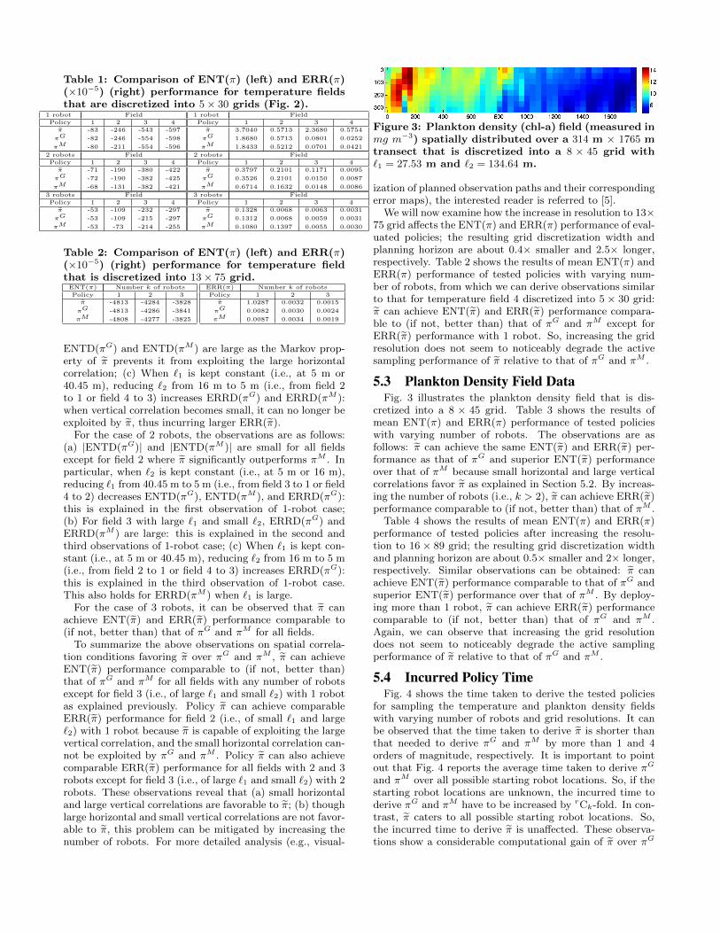
Table 1: Comparison of ENT(π) (left) and ERR(π)(×10−5) (right) performance for temperature fieldsthat are discretized into 5× 30 grids (Fig. 2).

1 robot Field

Policy 1 2 3 4

π -83 -246 -543 -597

πG -82 -246 -554 -598

πM -80 -211 -554 -596

1 robot Field

Policy 1 2 3 4

π 3.7040 0.5713 2.3680 0.5754

πG 1.8680 0.5713 0.0801 0.0252

πM 1.8433 0.5212 0.0701 0.0421

2 robots Field

Policy 1 2 3 4

π -71 -190 -380 -422

πG -72 -190 -382 -425

πM -68 -131 -382 -421

2 robots Field

Policy 1 2 3 4

π 0.3797 0.2101 0.1171 0.0095

πG 0.3526 0.2101 0.0150 0.0087

πM 0.6714 0.1632 0.0148 0.0086

3 robots Field

Policy 1 2 3 4

π -53 -109 -232 -297

πG -53 -109 -215 -297

πM -53 -73 -214 -255

3 robots Field

Policy 1 2 3 4

π 0.1328 0.0068 0.0063 0.0031

πG 0.1312 0.0068 0.0059 0.0031

πM 0.1080 0.1397 0.0055 0.0030

Table 2: Comparison of ENT(π) (left) and ERR(π)(×10−5) (right) performance for temperature fieldthat is discretized into 13× 75 grid.ENT(π) Number k of robots

Policy 1 2 3

π -4813 -4284 -3828

πG -4813 -4286 -3841

πM -4808 -4277 -3825

ERR(π) Number k of robots

Policy 1 2 3

π 1.0287 0.0032 0.0015

πG 0.0082 0.0030 0.0024

πM 0.0087 0.0034 0.0019

ENTD(πG) and ENTD(πM ) are large as the Markov prop-erty of π prevents it from exploiting the large horizontalcorrelation; (c) When `1 is kept constant (i.e., at 5 m or40.45 m), reducing `2 from 16 m to 5 m (i.e., from field 2to 1 or field 4 to 3) increases ERRD(πG) and ERRD(πM ):when vertical correlation becomes small, it can no longer beexploited by π, thus incurring larger ERR(π).

For the case of 2 robots, the observations are as follows:(a) |ENTD(πG)| and |ENTD(πM )| are small for all fieldsexcept for field 2 where π significantly outperforms πM . Inparticular, when `2 is kept constant (i.e., at 5 m or 16 m),reducing `1 from 40.45 m to 5 m (i.e., from field 3 to 1 or field4 to 2) decreases ENTD(πG), ENTD(πM ), and ERRD(πG):this is explained in the first observation of 1-robot case;(b) For field 3 with large `1 and small `2, ERRD(πG) andERRD(πM ) are large: this is explained in the second andthird observations of 1-robot case; (c) When `1 is kept con-stant (i.e., at 5 m or 40.45 m), reducing `2 from 16 m to 5 m(i.e., from field 2 to 1 or field 4 to 3) increases ERRD(πG):this is explained in the third observation of 1-robot case.This also holds for ERRD(πM ) when `1 is large.

For the case of 3 robots, it can be observed that π canachieve ENT(π) and ERR(π) performance comparable to(if not, better than) that of πG and πM for all fields.

To summarize the above observations on spatial correla-tion conditions favoring π over πG and πM , π can achieveENT(π) performance comparable to (if not, better than)that of πG and πM for all fields with any number of robotsexcept for field 3 (i.e., of large `1 and small `2) with 1 robotas explained previously. Policy π can achieve comparableERR(π) performance for field 2 (i.e., of small `1 and large`2) with 1 robot because π is capable of exploiting the largevertical correlation, and the small horizontal correlation can-not be exploited by πG and πM . Policy π can also achievecomparable ERR(π) performance for all fields with 2 and 3robots except for field 3 (i.e., of large `1 and small `2) with 2robots. These observations reveal that (a) small horizontaland large vertical correlations are favorable to π; (b) thoughlarge horizontal and small vertical correlations are not favor-able to π, this problem can be mitigated by increasing thenumber of robots. For more detailed analysis (e.g., visual-

Figure 3: Plankton density (chl-a) field (measured inmg m−3) spatially distributed over a 314 m × 1765 mtransect that is discretized into a 8 × 45 grid with`1 = 27.53 m and `2 = 134.64 m.

ization of planned observation paths and their correspondingerror maps), the interested reader is referred to [5].

We will now examine how the increase in resolution to 13×75 grid affects the ENT(π) and ERR(π) performance of eval-uated policies; the resulting grid discretization width andplanning horizon are about 0.4× smaller and 2.5× longer,respectively. Table 2 shows the results of mean ENT(π) andERR(π) performance of tested policies with varying num-ber of robots, from which we can derive observations similarto that for temperature field 4 discretized into 5 × 30 grid:π can achieve ENT(π) and ERR(π) performance compara-ble to (if not, better than) that of πG and πM except forERR(π) performance with 1 robot. So, increasing the gridresolution does not seem to noticeably degrade the activesampling performance of π relative to that of πG and πM .

5.3 Plankton Density Field DataFig. 3 illustrates the plankton density field that is dis-

cretized into a 8 × 45 grid. Table 3 shows the results ofmean ENT(π) and ERR(π) performance of tested policieswith varying number of robots. The observations are asfollows: π can achieve the same ENT(π) and ERR(π) per-formance as that of πG and superior ENT(π) performanceover that of πM because small horizontal and large verticalcorrelations favor π as explained in Section 5.2. By increas-ing the number of robots (i.e., k > 2), π can achieve ERR(π)performance comparable to (if not, better than) that of πM .

Table 4 shows the results of mean ENT(π) and ERR(π)performance of tested policies after increasing the resolu-tion to 16 × 89 grid; the resulting grid discretization widthand planning horizon are about 0.5× smaller and 2× longer,respectively. Similar observations can be obtained: π canachieve ENT(π) performance comparable to that of πG andsuperior ENT(π) performance over that of πM . By deploy-ing more than 1 robot, π can achieve ERR(π) performancecomparable to (if not, better than) that of πG and πM .Again, we can observe that increasing the grid resolutiondoes not seem to noticeably degrade the active samplingperformance of π relative to that of πG and πM .

5.4 Incurred Policy TimeFig. 4 shows the time taken to derive the tested policies

for sampling the temperature and plankton density fieldswith varying number of robots and grid resolutions. It canbe observed that the time taken to derive π is shorter thanthat needed to derive πG and πM by more than 1 and 4orders of magnitude, respectively. It is important to pointout that Fig. 4 reports the average time taken to derive πG

and πM over all possible starting robot locations. So, if thestarting robot locations are unknown, the incurred time toderive πG and πM have to be increased by rCk-fold. In con-trast, π caters to all possible starting robot locations. So,the incurred time to derive π is unaffected. These observa-tions show a considerable computational gain of π over πG

1 2 310−5

10−4

10−3

10−2

10−1

100

k

Tim

e (s

)

!

!G

!M

~

(a)1 2 3

10−4

10−2

100

102

104

k

Tim

e (s

)

!

!G

!M

~

(b)1 2 3 4

10−4

10−2

100

102

k

Tim

e (s

)

!

!G

!M(c)

~

1 2 310−4

10−2

100

102

104

106

k

Tim

e (s

)

!

!G

!M(d)

~

Figure 4: Graph of time taken to derive policy vs. number k of robots for temperature field 4 discretizedinto (a) 5× 30 and (b) 13× 75 grids and plankton density field discretized into (c) 8× 45 and (d) 16× 89 grids.

Table 3: Comparison of ENT(π) (left) and ERR(π)(×10−3) (right) performance for plankton densityfield that is discretized into 8× 45 grid.

ENT(π) Number k of robots

Policy 1 2 3 4

π -359 -322 -196 -121

πG -359 -322 -196 -121

πM -230 -186 -70 -11

ERR(π) Number k of robots

Policy 1 2 3 4

π 5.6124 2.2164 0.0544 0.0066

πG 5.6124 2.2164 0.0544 0.0066

πM 4.5371 0.5613 0.0472 0.0324

Table 4: Comparison of ENT(π) (left) and ERR(π)(×10−3) (right) performance for plankton densityfield that is discretized into 16× 89 grid.ENT(π) Number k of robots

Policy 1 2 3

π -4278 -3949 -3681

πG -4238 -3964 -3686

πM -4171 -3840 -3501

ERR(π) Number k of robots

Policy 1 2 3

π 3.4328 0.0970 0.0546

πG 1.5648 0.1073 0.0643

πM 0.8186 0.0859 0.0348

and πM , which supports our time complexity analysis andcomparison (Section 4). So, our Markov-based path planneris more time-efficient for in situ, real-time, high-resolutionactive sampling.

6. CONCLUSIONThis paper describes an efficient Markov-based information-

theoretic path planner for active sampling of GP-based en-vironmental fields. We have provided theoretical guaranteeson the active sampling performance of our Markov-basedpolicy π for the transect sampling task, from which idealenvironmental field conditions (i.e., small horizontal spatialcorrelation and noisy, less intense fields) and sampling tasksettings (i.e., large grid discretization width and short plan-ning horizon) can be established to limit its performancedegradation. Empirically, we have shown that π can gen-erally achieve active sampling performance comparable tothat of the widely-used non-Markovian greedy policies πG

and πM under less favorable realistic field conditions (i.e.,low noise-to-signal ratio) and task settings (i.e., small griddiscretization width and long planning horizon) while en-joying huge computational gain over them. In particular,we have empirically observed that (a) small horizontal andlarge vertical correlations strongly favor π; (b) though largehorizontal and small vertical correlations do not favor π,this problem can be mitigated by increasing the number ofrobots. In fact, deploying a large robot team often producessuperior active sampling performance of π over πM in ourexperiments, not forgetting the computational gain of > 4orders of magnitude. Our Markov-based planner can be usedto efficiently achieve more general exploration tasks (e.g.,boundary tracking and those in [6, 7]), but the guaranteesprovided here may not apply. For our future work, we will“relax” the Markov assumption by utilizing a longer (butnot entire) history of observations in path planning. Thiscan potentially improve the active sampling performance in

fields of moderate to large horizontal correlation but doesnot incur as much time as that of non-Markovian policies.

7. REFERENCES[1] G. H. Golub and C.-F. Van Loan. Matrix

Computations. Johns Hopkins Univ. Press, 3rdedition, 1996.

[2] R. Korf. Real-time heuristic search. Artif. Intell.,42(2-3):189–211, 1990.

[3] A. Krause, A. Singh, and C. Guestrin. Near-optimalsensor placements in Gaussian processes: Theory,efficient algorithms and empirical studies. JMLR,9:235–284, 2008.

[4] N. E. Leonard, D. Paley, F. Lekien, R. Sepulchre,D. M. Fratantoni, and R. Davis. Collective motion,sensor networks and ocean sampling. Proc. IEEE,95(1):48–74, 2007.

[5] K. H. Low. Multi-Robot Adaptive Exploration andMapping for Environmental Sensing Applications.Ph.D. Thesis, Technical Report CMU-ECE-2009-024,Department of Electrical and Computer Engineering,Carnegie Mellon University, Pittsburgh, PA, 2009.

[6] K. H. Low, J. M. Dolan, and P. Khosla. Adaptivemulti-robot wide-area exploration and mapping. InProc. AAMAS, pages 23–30, 2008.

[7] K. H. Low, J. M. Dolan, and P. Khosla.Information-theoretic approach to efficient adaptivepath planning for mobile robotic environmentalsensing. In Proc. ICAPS, pages 233–240, 2009.

[8] C. E. Rasmussen and C. K. I. Williams. GaussianProcesses for Machine Learning. MIT Press,Cambridge, MA, 2006.

[9] D. L. Rudnick, R. E. Davis, C. C. Eriksen,D. Fratantoni, and M. J. Perry. Underwater gliders forocean research. Mar. Technol. Soc. J., 38(2):73–84,2004.

[10] M. C. Shewry and H. P. Wynn. Maximum entropysampling. J. Applied Stat., 14(2):165–170, 1987.

[11] A. Stahl, Ringvall, and T. Lamas. Guided transectsampling for assessing sparse populations. ForestScience, 46(1):108–115, 2000.

[12] G. W. Stewart and J.-G. Sun. Matrix PerturbationTheory. Academic Press, 1990.

[13] D. R. Thompson and D. Wettergreen. Intelligent mapsfor autonomous kilometer-scale science survey. InProc. i-SAIRAS, 2008.

[14] S. Thrun, W. Burgard, and D. Fox. ProbabilisticRobotics. MIT Press, Cambridge, MA, 2005.

[15] R. Webster and M. Oliver. Geostatistics for

Environmental Scientists. John Wiley & Sons, Inc.,NY, 2nd edition, 2007.

APPENDIXA. PROOFS

A.1 Proof Sketch of Theorem 1For each vector xi of current robot locations, the time

needed to evaluate the posterior entropy H[Zτ(xi,ai)|Zxi ](i.e., using Cholesky factorization) over all possible actionsai ∈ A(xi) is |A| × O(k4) = O(|A|k4). Doing this over allpossible vectors of current robot locations in each columnthus incurs |A|×O(|A|k4) = O(|A|2k4) time since the vectorspace of current robot locations in each column is of the samesize as that of the joint action space |A|. We do not haveto compute these posterior entropies again for every columnbecause the entropies evaluated for any one column repli-cate across different columns. This computational saving isdue to the Markov assumption and the problem structure ofthe transect sampling task. Propagating the optimal valuesfrom stages t to 0 takes O(|A|2t) time. Hence, solving theMarkov-based path planning problem (11) or deriving theMarkov-based policy π (12) takes O(|A|2(t + k4)) time forthe transect sampling task.

A.2 Proof of Lemma 2Let Σx0:i−1x0:i−1|xi

4= C + E where C is defined to be a

matrix with diagonal components σ2xk = σ2

s + σ2n for k =

0, . . . , i− 1 and off-diagonal components 0, and E is definedto be a matrix with diagonal components −(σxkxi)

2/σ2xi =

−(σxkxi)2/(σ2

s + σ2n) for k = 0, . . . , i − 1 and the same

off-diagonal components as Σx0:i−1x0:i−1|xi (i.e., σxjxk|xi =

σxjxk − σxjxiσxixk/σ2xi for j, k = 0, . . . , i− 1, j 6= k). Then,

||C−1||2 = ||(σ2s + σ2

n)−1I||2 =1

σ2s + σ2

n

. (15)

The last equality follows from σ2s + σ2

n being the smallesteigenvalue of C. So, 1/(σ2

s + σ2n) is the largest eigenvalue of

C−1, which is equal to ||C−1||2.Note that the minimum distance between any pair of lo-

cation components of x0:i−1 cannot be less than ω1. So, itcan be observed that any component of E cannot have anabsolute value more than σ2

sξ. Therefore,

||E||2 ≤ iσ2sξ , (16)

which follows from a property of the matrix 2-norm that||E||2 cannot be more than the largest absolute componentof E multiplied by i [1].

Note that the minimum distance between locations xi andxi+1 as well as between location xi and any location compo-nent of x0:i−1 cannot be less than ω1. So, it can be observedthat any component of Σxi+1x0:i−1|xi cannot have an abso-

lute value more than σ2sξ

2. Therefore,

|σZxi+1Zxk |xi

| ≤ σ2sξ

2 (17)

for k = 0, . . . , i− 1.

Now,

Σxi+1x0:i−1|xi(C + E)−1Σx0:i−1xi+1|xi −Σxi+1x0:i−1|xiC

−1Σx0:i−1xi+1|xi

= Σxi+1x0:i−1|xi{(C + E)−1 − C−1}Σx0:i−1xi+1|xi

≤ ||Σxi+1x0:i−1|xi ||22 ||(C + E)−1 − C−1||2

≤i−1∑k=0

|σZxi+1Zxk |xi

|2 ||C−1||2 ||E||21

||C−1||2− ||E||2

= i(σ2s)2ξ4

||C−1||2 ||E||21

||C−1||2− ||E||2

.

(18)

The first inequality is due to Cauchy-Schwarz inequality andsubmultiplicativity of the matrix norm [12]. The second in-equality follows from an important result in the perturba-tion theory of matrix inverses (in particular, Theorem III.2.5in [12]). It requires the assumption of ||C−1 E||2 < 1.This assumption can be satisfied by ||C−1||2 ||E||2 < 1because ||C−1 E||2 ≤ ||C−1||2 ||E||2. By (15) and (16),||C−1||2 ||E||2 < 1 translates to ξ < ρ/i. The last equalityis due to (17).

From (18),

Σxi+1x0:i−1|xi(C + E)−1Σx0:i−1xi+1|xi

≤ Σxi+1x0:i−1|xiC−1Σx0:i−1xi+1|xi + i(σ2

s)2ξ4||C−1||2 ||E||2

1||C−1||2

− ||E||2

≤ i(σ2s)2ξ4 ||C−1||2

(1 +

||E||21

||C−1||2− ||E||2

)

=i(σ2

s)2ξ4

1||C−1||2

− ||E||2

≤ i(σ2s)2ξ4

σ2s + σ2

n − iσ2sξ

=σ2sξ

4

ρi− ξ

(19)The second inequality is due to

Σxi+1x0:i−1|xiC−1Σx0:i−1xi+1|xi ≤ i(σ

2s)2ξ4 ||C−1||2 ,

which follows from Cauchy-Schwarz inequality and (17). Thethird inequality follows from (15) and (16).

We will need the following property of posterior variancethat is similar to (3):

σ2xi+1|x0:i = σ2

xi+1|xi−Σxi+1x0:i−1|xiΣ−1x0:i−1x0:i−1|xiΣx0:i−1xi+1|xi

(20)where Σxi+1x0:i−1|xi is a posterior covariance vector withcomponents σxi+1xk|xi for k = 0, . . . , i − 1, Σx0:i−1xi+1|xiis the transpose of Σxi+1x0:i−1|xi , and Σx0:i−1x0:i−1|xi is aposterior covariance matrix with components σxjxk|xi forj, k = 0, . . . , i− 1.

By (19) and (20),

σ2xi+1|xi − σ

2xi+1|x0:i

= Σxi+1x0:i−1|xiΣ−1x0:i−1x0:i−1|xi

Σx0:i−1xi+1|xi

≤ σ2sξ

4

ρi− ξ .

A.3 Proof of Theorem 4Proof by induction on i that V π

∗i (x0:i) ≤ Vi(xi) ≤ V π

∗i (x0:i) +∑t

s=i ∆(s) for i = t, . . . , 0.

Base case (i = t): By Lemma 3,

H[Zxt+1 |Zx0:t ] ≤ H[Zxt+1 |Zxt ]≤ H[Zxt+1 |Zx0:t ] + ∆(t) for any xt+1

⇒ maxat∈A(xt)

H[Zxt+1 |Zx0:t ] ≤ maxat∈A(xt)

H[Zxt+1 |Zxt ]

≤ maxat∈A(xt)

H[Zxt+1 |Zx0:t ] + ∆(t)

⇒ V π∗

t (x0:t) ≤ Vt(xt) ≤ V π∗

t (x0:t) + ∆(t) .(21)

Hence, the base case is true.

Inductive case: Suppose that

V π∗

i+1(x0:i+1) ≤ Vi+1(xi+1) ≤ V π∗

i+1(x0:i+1)+

t∑s=i+1

∆(s) (22)

is true. We have to prove that V π∗

i (x0:i) ≤ Vi(xi) ≤ V π∗

i (x0:i) +∑ts=i ∆(s) is true.

We will first show that Vi(xi) ≤ V π∗

i (x0:i) +∑ts=i ∆(s).

By Lemma 3,

H[Zxi+1 |Zxi ] ≤ H[Zxi+1 |Zx0:i ] + ∆(i) for any xi+1

⇒ H[Zxi+1 |Zxi ] + Vi+1(xi+1) ≤ H[Zxi+1 |Zx0:i ] +

V π∗

i+1(x0:i+1) +∑ts=i ∆(s) by (22) for any xi+1

⇒ maxai∈A(xi)

H[Zxi+1 |Zxi ] + Vi+1(xi+1)

≤ maxai∈A(xi)

H[Zxi+1 |Zx0:i ] + V π∗

i+1(x0:i+1) +

t∑s=i

∆(s)

⇒ Vi(xi) ≤ V π∗

i (x0:i) +

t∑s=i

∆(s) .

We will now prove that V π∗

i (x0:i) ≤ Vi(xi). By Lemma 3,

H[Zxi+1 |Zx0:i ] ≤ H[Zxi+1 |Zxi ] for any xi+1

⇒ H[Zxi+1 |Zx0:i ] + V π∗

i+1(x0:i+1)

≤ H[Zxi+1 |Zxi ] + Vi+1(xi+1) by (22) for any xi+1

⇒ maxai∈A(xi)

H[Zxi+1 |Zx0:i ] + V π∗

i+1(x0:i+1)

≤ maxai∈A(xi) H[Zxi+1 |Zxi ] + Vi+1(xi+1)

⇒ V π∗

i (x0:i) ≤ Vi(xi) .

Hence, the inductive case is true.

A.4 Proof of Theorem 5The following lemma is needed for this proof:

Lemma 7. Vi(xi) ≤ V πi (x0:i)+∑ts=i ∆(s) for i = 0, . . . , t.

The proof of the above lemma is provided in Appendix A.6.Proof by induction on i that V π

∗i (x0:i) ≤ V πi (x0:i)+

∑ts=i ∆(s)

for i = t, . . . , 0.

Base case (i = t):

V π∗

t (x0:t) ≤ Vt(xt) ≤ V πt (x0:t) + ∆(t) .

The first inequality is due to Theorem 4. The second in-equality follows from Lemma 7. Hence, the base case is true.

Inductive case: Suppose that

V π∗

i+1(x0:i+1) ≤ V πi+1(x0:i+1) +

t∑s=i+1

∆(s) (23)

is true. We have to prove that V π∗

i (x0:i) ≤ V πi (x0:i) +∑ts=i ∆(s) is true.

V π∗

i (x0:i) ≤ Vi(xi)= H[Zτ(xi,πi(xi))|Zxi ] + Vi+1(τ(xi, πi(xi)))

≤ H[Zτ(xi,πi(xi))|Zx0:i ] + ∆(i) + Vi+1(τ(xi, πi(xi)))

≤ H[Zτ(xi,πi(xi))|Zx0:i ] + ∆(i) + V πi+1( (x0:i, τ(xi, πi(xi))) ) +∑ts=i+1 ∆(s)

= V πi (x0:i) +

t∑s=i

∆(s) .

The first inequality is due to Theorem 4. The first equal-ity follows from (11). The second inequality follows fromLemma 3. The third inequality is due to Lemma 7. The lastequality follows from (5). Hence, the inductive case is true.

A.5 Proof Sketch of Lemma 6Define x

[m]i to be the m-th component of vector xi of robot

locations for m = 1, . . . , k. Let x[1:m]i denote a vector com-

prising the first m components of xi (i.e., concatenation of

x[1]i , . . . , x

[m]i ).

I[Zxi+1 ;Zx0:i−1 |Zxi ]= H[Zxi+1 |Zxi ]−H[Zxi+1 |Zx0:i ]

=

k∑m=1

(H[Z

x[m]i+1

|Z(xi,x

[1:m−1]i+1 )

]−H[Zx[m]i+1

|Z(x0:i,x

[1:m−1]i+1 )

]

)

=1

2

k∑m=1

log

σ2

x[m]i+1|(xi,x

[1:m−1]i+1 )

σ2

x[m]i+1|(x0:i,x

[1:m−1]i+1 )

=

1

2

k∑m=1

log

1−σ2

x[m]i+1|(xi,x

[1:m−1]i+1 )

− σ2

x[m]i+1|(x0:i,x

[1:m−1]i+1 )

σ2

x[m]i+1|(xi,x

[1:m−1]i+1 )

−1

≥ 0 .(24)

The second equality follows from the chain rule for entropy.Similar to Lemma 2, the following result bounds the vari-

ance reduction term

σ2

x[m]i+1|(xi,x

[1:m−1]i+1 )

− σ2

x[m]i+1|(x0:i,x

[1:m−1]i+1 )

in (24):

Lemma 8. If ξ < min(ρ

ik,ρ

4k) and (14) is satisfied,

0 ≤ σ2

x[m]i+1|(xi,x

[1:m−1]i+1 )

− σ2

x[m]i+1|(x0:i,x

[1:m−1]i+1 )

≤ σ2sξ

4

ρik− ξ .

The proof of the above result is largely similar to that ofLemma 2 (Appendix A.2), and is therefore omitted here.

The bounds on I[Zxi+1 ;Zx0:i−1 |Zxi ] follow immediatelyfrom (24), Lemma 8, and the following lower bound on

σ2

x[m]i+1|(xi,x

[1:m−1]i+1 )

:

σ2

x[m]i+1|(xi,x

[1:m−1]i+1 )

= σ2

x[m]i+1

−

Σx[m]i+1(xi,x

[1:m−1]i+1 )

Σ−1

(xi,x[1:m−1]i+1 )(xi,x

[1:m−1]i+1 )

Σ(xi,x

[1:m−1]i+1 )x

[m]i+1

≥ σ2s + σ2

n −σ2sξ

2

ρ2k−1

− ξ≥ σ2

s + σ2n − 4k

ρσ2sξ

2 .

The equality is due to (3). The first inequality is due toCauchy-Schwarz inequality, submultiplicativity of the ma-trix norm [12], and a result in the perturbation theory ofmatrix inverses (in particular, Theorem III.2.5 in [12]). Thesecond inequality follows from the given satisfied condition

ξ <ρ

4k.

A.6 Proof of Lemma 7Proof by induction on i that Vi(xi) ≤ V πi (x0:i)+

∑ts=i ∆(s)

for i = t, . . . , 0.

Base case (i = t):

Vt(xt) = maxat∈A(xt)

H[Zτ(xt,at)|Zxt ]

= H[Zτ(xt,πt(xt))|Zxt ]≤ H[Zτ(xt,πt(xt))|Zx0:t ] + ∆(t)

= V πt (x0:t) + ∆(t) .

The first equality follows from (11). The inequality followsfrom Lemma 3. The last equality is due to (5). So, the basecase is true.

Inductive case: Suppose that

Vi+1(xi+1) ≤ V πi+1(x0:i+1) +

t∑s=i+1

∆(s) (25)

is true. We have to prove that Vi(xi) ≤ V πi (x0:i)+∑ts=i ∆(s)

is true.By Lemma 3,

H[Zxi+1 |Zxi ] ≤ H[Zxi+1 |Zx0:i ] + ∆(i) for any xi+1

⇒ H[Zxi+1 |Zxi ] + Vi+1(xi+1) ≤ H[Zxi+1 |Zx0:i ] +

V πi+1(x0:i+1) +∑ts=i ∆(s) by (25) for any xi+1

⇒ H[Zτ(xi,πi(xi))|Zxi ] + Vi+1(τ(xi, πi(xi)))

≤ H[Zτ(xi,πi(xi))|Zx0:i ] + V πi+1( (x0:i, τ(xi, πi(xi))) ) +∑ts=i ∆(s)by xi+1 ← τ(xi, πi(xi))

⇒ Vi(xi) ≤ V πi (x0:i) +t∑s=i

∆(s) by (11) and (5).

Hence, the inductive case is true.