activities of the sub-working group on data...

Activities of the sub-working group on

data homogenization

Roeland Van Malderen, Royal Meteorological Institute of Belgium (RMI) - Solar-Terrestrial Centre of Excellence (STCE)

Eric Pottiaux, Royal Observatory of Belgium (ROB) – Solar-Terrestrial Centre of Excellence (STCE)

and many others

Royal Observatory

of Belgium

Solar-Terrestrial Centre

of Excellence

Outline

Context and Primary Objectives

The reference dataset and its reference

The first homogenization workshop at Brussels

2

Context

From different presentations at different GNSS4SWEC workshops, it turned out that different groups were showing results from time series

analyses, sometimes based on the same datasets.

They were dealing/struggling with the homogenization of their datasets.

A need for a common activity? send an EoI (22 responses) + Inquiry

(17 participants).

3

Objectives

1. To work on one or two long-term reference datasets.

We start with the IGS repro 1 troposphere products screened and converted to IWV by O. Bock.

2. To work with different homogenization methods/ algorithms:

To inter-compare their results, advantages, drawbacks…

To build a list of commonly identified inhomogeneities (instrumental change, break points, auxiliary data jumps…).

3. To come up with an homogenized version of the reference dataset that can be re-used to study climate trends and time variability by the community.

4

5 IGS Repro 1: 120 stations with data from 1995-2010

From A. Klos

Important note

ERA-interim is used to screen

the ZTD IGS repro 1 data

To convert ZTD to IWV, ERA-

interim is used

Surface pressure of ERA-

interim

Weighted mean temperature

calculated from pressure

levels

6 Good correlation between IGS Repro 1 and ERA-interim

From O. Bock

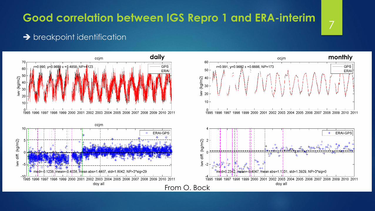
breakpoint identification

7 Good correlation between IGS Repro 1 and ERA-interim

daily monthly

From O. Bock

Dedicated Workshop in Brussels 8

10 Participants from our Action (not all could come) + 1 External Expert (E. Aguilar)

Dedicated Workshop in Brussels 9

Ning Bock et al. KTU (Tanır Kayıkçı-Zengin Kazancı)

monthly monthly daily monthly daily daily daily manual

albh 15/10/2002 15/10/2002 2/05/1998 18/05/2002

albh 15/03/2000 9/07/1998

albh 15/02/2006 2/07/2000

albh 12/03/2001

albh 18/01/2005

algo 7/02/2008 17/05/1997 12/10/2007 1

alic 20/04/2006 15/04/2006 15/04/2006 21/08/1999 26/10/2008 31/07/1999 1

alic 15/08/1999 15/08/1999 20/04/2006 15/06/2003 1

alic 6/05/2010 1

alic 11/10/1999 3

ankr 15/09/2000 15/10/2001 15/10/2001 15/10/2001 15/10/2001 3/01/2001 18/05/2005 7/02/1996 1

ankr 15/08/2000 15/09/2000 11/05/2008 23/07/1996 1

ankr 15/09/2008 15/09/2008 24/07/1997 1

ankr 16/09/1998 1

ankr 4/07/2000 1

ankr 24/11/2000 1

ankr 6/05/2008 1

ankr 4/06/1999 3

ankr 16/09/2000 3

ankr 26/11/2007 3

Elias Van Malderen et al. Klos et al.

Dedicated workshop in Brussels

breakpoints detected in metadata & visual inspection, but not by any of the groups?

breakpoints detected by a number (all) tools, but no metadata

information?

time window! When are breakpoints coincident?

Based on the expertise of E. Aguilar, we decided to focus first on the

generation of a synthetic dataset in which known offsets are

inserted (Anna Klos) and to collect as much as possible (“trustable”)

meta-data, before trying to homogenize our reference IGS repro 1

dataset.

10

Results of the homogenization tools

on the synthetic benchmark IWV

datasets

Roeland Van Malderen, Royal Meteorological Institute of Belgium (RMI) - Solar-Terrestrial Centre of Excellence (STCE) Eric Pottiaux, Royal Observatory of Belgium (ROB) – Solar-Terrestrial Centre of Excellence (STCE) Anna Klos, Military University of Technology, Warsaw, Poland

Olivier Bock, IGN LAREG, University Paris Diderot, Sorbonne Paris, France Janusz Bogusz, Military University of Technology, Warsaw, Poland Barbara Chimani, Central Institute for Meteorology and Geodynamics, Austria Michal Elias, Research Institute of Geodesy, Topography and Cartography, Czech Republic Marta Gruszczynska, Military University of Technology, Warsaw, Poland José Guijarro, AEMET (Spanish Meteorological Agency), Spain

Selma Zengin Kazancı, Karadeniz Technical University, Turkey Tong Ning, Lantmäteriet, Sweden

Royal Observatory

of Belgium


of Excellence

Dedicated Workshop in Warsaw 12

12 participants from our Action + 2 “HOME” experts (B. Chimani + J. Guijarro)

MUT, 23-25 January 2017

scope:

analysis of the

results of different tools on the

synthetic datasets

Summary of the different tools 13

Climatol J. Guijarro

HOMOP B. Chimani

PMTred T. Ning

Non-parametric tests

R. Van Malderen

2-sample t-statistic

M. Elias

Pettitt test

S. Zengin Kazancı, E. Tanir Kayikçi, V.

Tornatore

14 participants 6 different homogenization tools

Summary of the different tools 14

Climatol J. Guijarro

Non-parametric tests

R. Van Malderen

Neighbor-based, based on orthogonal regression between standardized anomalies (x-μx)/σx and (y- μy)/σy.

Missing data are filled in, outliers removed.

Varying amplitude of the corrected offsets (by including e.g. σx in the standardization, you might include seasonality in the amplitudes).

The Standard Normal Homogeneity Test (SNHT) to find shifts in the mean is applied to the anomaly series in two stages.

Detection of multiple change points by applying the test to the remaining segments.

Runs on daily values, but might be also applied for monthly data.

Non-parametric distributional tests that utilize ranks: the Mann-Whitney-Wilcoxon test and the Pettitt-Mann-Whitney test.

The CUSUM test (based on the sum of the deviations from the mean) is also used an additional reference.

Iterative procedure: if 2 out of those 3 tests identify a statistical significant breakpoint, the time series is corrected and the tests are applied again on the complete corrected time series.

Runs on monthly and daily values.

Homogenization Methods and

Contributions Available

Method 1 Method 2 Method 3 Method 4 Method 5 Method 6 Method 7

Operator M. Elias R. Van

Malderen

R. Van

Malderen

J. Guijarro T. Ning S. Zengin B. Chimani

Method / SW PMTred 2 of 3 PMW CLIMATOL PMTred Pettitt HOMOP

Daily/Monthly D+M D+M D+M D+M D+M D X

Easy/Less/Full E+L+F E+L+F E+L+F L+F E+L+F E+L+F E+F

15

in the pipeline: P. Stepanek, O. Bock, M. Gruszczynska, manual detection?

We welcome other contributions (e.g. SSA at GFZ talk by Fadwa Alshawaf)

also possible: try running existing homogenization tools (e.g. HOMER)

Assessment of the performance of the

tools …

16

… on the identification of the epochs of the inserted breakpoints (+

sensitivity analysis) in the synthetic datasets.

work done by Eric Pottiaux, Anna Klos & Janusz Bogusz, next talk by Eric.

… on the estimation of the trends that were or were not imposed to the 3

sets of synthetic IWV differences.

work done by Anna Klos & Janusz Bogusz, presented by me.

Deriving Error Metrics for the Homogenization

of Integrated Water Vapour (IWV) Time Series: THE CASE OF THE SYNTHETIC BENCHMARK DATASETS.


Anna Klos, Military University of Technology (MUT)

Roeland Van Malderen, Royal Meteorological Institute of Belgium (RMI) – Solar-Terrestrial Centre of Excellence (STCE)

Janusz Bogusz, Military University of Technology, Warsaw, Poland

Elias Michal, Geodetic Observatory Pecny (GOP)

Jose A. Guijarro, Spanish Meteorological Agency

Tong Ning, Lantmateriett, Sweden

Barbara Chimani, ZAMG

Selma Zengin Kazanci, Karadeniz Technical University, Trabzon

Royal Observatory

of Belgium


of Excellence

Deriving Error Metrics for the

Homogenization of IWV Time Series METHODOLOGY AND CONTRIBUTIONS

18

Global Methodology for Performance

Assessment

19

BLIND “Data Homogenization”

‘”EASY” ‘”LESS” ‘”FULLY”

Increasing Complexity

Daily Values

Monthly Values

Homogenization Method 1



Homogenization Method N

…

IGS repro 1 Characteristics

ERA-Interim Characteristics

“Truth”

Result Set 1

Result Set 2

Result Set 3

Result Set N

…

Feedback & Enhancement Loop

Synthetic datasets

‘True’ datasets

Summary of Results Contributions 20

Results from Barbara Chimani not yet handled (technical reason) Three more contributors expected (Olivier Bock, Petr Stepanek, Yingbo Li) – More are welcome !

9

11

13

4

5 5 5

6

7

0

2

4

6

8

10

12

14

EASY LESS FULL

Submission Info. w.r.t. Synthetic Dataset Type

Nb of result datasets used Nb. Of Contributors Included Nb. of Methods Used


Homogenization of IWV Time Series METRICS FOR SENSITIVITY AND PERFORMANCE ASSESSMENT

21

Type of Metrics 22

Venema et al. (2012), Benchmarking homogenization algorithms for monthly data, Climate of the Past, 8, 89-115, doi:10.5194/cp-8-89-2012, 2012

(http://www.clim-ast.net/8/89/2012/).

Lev

el 1

.a

Lev

el 1

.b

Lev

el 2

e.g. number of Hits, Misses, …

Statistical Scores

e.g. the Probability of Detection,

False Alarm Rate, Critical Success Index, Pierce Skill Score

Probabilistic and Skill Scores

e.g. impact on trend estimates and their uncertainties

Tailored Metrics (focused on App)

http://www.clim-ast.net/8/89/2012/





4 Basic Statistical Scores

True Positive (TP) – “Hits”

“offset reported by the homogenization method which corresponds to a true synthetic offset within

a certain time window“

True Negative (TN) – “no break present, nor predicted”

“no offset reported by the homogenization method

when no offset was inserted in the synthetic dataset”

False Positive (FP) – “False Alarms”

“offset reported by the homogenization method when no offset was inserted in the synthetic

dataset”

False Negative (FN) – “misses”

“no offset reported by the homogenization method while an offset was inserted in the synthetic

dataset”

“Accuracy of Detection”

23

The 4 Basic Statistical Scores by Example 24

True Positive (TP) False Positive (FP) False Negative (FN)


True Negative (TN)


Need to define a proper time window for offset matches !!!

True Positive (TP) False Positive (FP) False Negative (FN)

Other examples: results from various tools 27

Need to define a proper time window for offset matches !!!

FULLY-COMPLICATED


Homogenization of IWV Time Series DEFINING THE PROPER TIME WINDOW

28

Time Window to Find “Matches” (TP)

To find potential matches between estimated offsets and the true

offsets inserted in the synthetic dataset, it is mandatory to fix some time

window.

29

Defining the proper Time Window

At the moment, it has been done quite empirically

Starting with a large time window of ±186 days (~ ±6 months) around the true offset epoch

Studying the distribution of epoch differences (estimated vs. truth)

30

[-186d,+186d]

Tru

e O

ffse

t

Defining the proper Time Window 31

Defining the proper Time Window 32

We decided (somehow arbitrary) that

A time window of 62 days is convenient for deriving metrics for both, daily

and monthly mean values from the synthetic datasets.

A time window of 31 days can be convenient when working with daily

values.


Homogenization of IWV Time Series HOW MUCH OFFSET ARE DETECTED VERSUS THE TRUE NUMBER ?

33

Number of Offset Estimated A

bso

lute

Va

lue

s

Ra

tio

Est

ima

ted

/Tru

e O

ffse

t N

b.

34

Number of Offset Estimated R

atio

Est

ima

ted

/Tru

e O

ffse

t N

b.

35

Number of Offset Estimated R

atio

Est

ima

ted

/Tru

e O

ffse

t N

b.

Ra

tio

Est

ima

ted

/Tru

e O

ffse

t N

b.

36


Homogenization of IWV Time Series QUESTIONS AND OBJECTIVES

37

Some Questions and Objectives

What is the sensitivity of the homogenization methods w.r.t.

•The complexity of the synthetic dataset, i.e. w.r.t.

•Addition of A.R. noise (from EASY to LESS)

•Addition of gaps and trend (from LESS to FULL)

•The ‘observation’ frequency of the time series (daily vs. monthly)

What are the performances of the homogenization methods w.r.t.

•The timing of the estimated offset epochs (accuracy)

•The amplitude of the estimated offsets (accuracy)

•To the geographical location (more/less TP/FP/FAR in some regions?)

•The station time series characteristics (noises, signals, gaps, trends correlation?)

•Edges vs. ‘inside’ of the station time series (e.g. ranking vs. T-test based methods)

38 Se

nsi

tivity

Fe

ed

ba

ck


Homogenization of IWV Time Series SENSITIVITY W.R.T. THE SYNTHETIC DATASET COMPLEXITY

39

Scores from the EASY Synthetic Dataset

Absolute Value Relative Percentage

40

Ternary Graphs Example 41

Performance Increase

Need to define performance

criteria, such as:

► True Positives + Negatives > 40 %

► False Negatives < 40%

► False Positives < 40%

Gazeaux et al. 2013, Detecting offsets in GPS time series: First results from the detection of offset in GPS experiment, JGR

Sensitivity w.r.t. to the Synthetic Dataset

Complexity

EASY LESS Complicated

42

+ A.R. Noise

Sensitivity w.r.t. to the Synthetic Dataset

Complexity

LESS Complicated FULLY Complicated

43

+ gap and trend


Homogenization of IWV Time Series FEEDBACK AND METHODOLOGY ENHANCEMENTS

44

Feedback : From Blind Homogenization

to Optimization

Releasing the ‘truth’ about the different synthetic dataset (already

done on demand for “EASY”) can help fine-tuning the homogenization

methods.

45


Homogenization of IWV Time Series FEEDBACK: ACCURACY OF THE TIMING OF THE ESTIMATED OFFSETS

46

EASY

LESS

FULLY

Accuracy of the Estimated Offset Epochs 47 W.r.t. the complexity of the synthetic dataset

De

cre

ase

d A

cc

ura

cy o

f th

e T

imin

g

Accuracy of the Estimated Offset Epochs

Easy Less Full

Da

ily

48

Decreased Accuracy of the Timing

W.r.t. the complexity of the synthetic dataset

Decreased Accuracy of the Timing

Accuracy of the Estimated Offset Epochs

Easy Less Full

Mo

nth

ly

Da

ily

49 W.r.t. daily versus monthly mean values from the synthetic dataset

Accuracy of the Estimated Offset Epochs 50 W.r.t. homogenization method

Accuracy of the Estimated Offset Epoch

Depends on

The complexity of the synthetic dataset.

The frequency of the synthetic dataset values (daily versus monthly means).

On the homogenization method.

51


Homogenization of IWV Time Series FEEDBACK: ACCURACY OF THE OFFSET AMPLITUDE ESTIMATED

52

Accuracy of the Estimated Offset Amplitude 53

Amplitudes of reported offsets

EASY (SIM: 291)

ME1: 199

RVM 2of3 M: 202

RVM 2of3 D: 252

RVM PMW M: 213

TN D: 216

TN M: 130


Amplitudes of reported offsets

FULLY-COMPLICATED (SIM: 317)

JG: 146

ME1: 170

ME2: 185

TN D: 264

TN M: 128

RVM 2of3 M: 238

RVM 2of3 D: 386

RVM PMW M: 260


With Gap Filling Without Gap Filling

► Slope quite close to a 1:1 relationship and even slightly closer when filling gap.

► Similar method, same operator but opposite sign (matter of convention, not too much of concerns for trends).


Monthly Daily

► Slope seems rather insensitive to daily versus monthly mean values (at least for this method).

► Systematic underestimation of the offset amplitude (related to the timing accuracy ?).


Homogenization of IWV Time Series FINDING THE ORIGINS OF PERFORMANCE DEGRADATIONS

57

Feedback : From Blind Homogenization

to Optimization

Ongoing work : more elaborated feedback like studying the sensitivity

of the performances w.r.t. the synthetic dataset characteristics using a

bi-variate correlation analysis :

Noise model, coefficient and amplitude

Signal Cycle (Annual, Semi-Annual, Ter-Annual, Quarter-Annual) amplitude and phase

Percentage of gaps

Trend (number and amplitude)

58

Example of Bi-Variate Correlation Analysis

Dataset: FD5

59

FAR versus Signal’s Amplitude and Phase


Homogenization of IWV Time Series TREND AND TREND UNCERTAINTIES AS PERFORMANCE METRICS

60

Methodology 1. For each of the provided solutions, we characterized the number of

epochs found and calculated the amplitudes of those offsets

(consistency!)

2. We corrected the time series with the amplitudes found and we run (HECTOR) the Maximum Likelihood Estimation (MLE) with the epochs

found by different tools.

3. We cross-compared the values of trend, seasonal signals and

parameters of noise when different epochs were applied.

61

The number, amplitudes and epochs of offsets may change:

1. Value of trend.

2. The character of the stochastic part trend uncertainty.

They will not affect:

Amplitudes of seasonal signals.

Changes in seasonals and noise

Maximum change in the annual amplitude of 0.1 mm.

Maximum change in coefficient of autoregressive noise of 0.2 (Less

complicated) & of 0.3 (Fully complicated).

62

Changes in trends 63

EASY

“Hector “ = output from MLE with simulated offsets


LESS COMPLICATED



FULLY COMPLICATED


Future ACTIVITIES OF THE SUB-WORKING GROUP ON DATA HOMOGENIZATION

Roeland Van Malderen, Royal Meteorological Institute of Belgium (RMI) - Solar-Terrestrial Centre of Excellence (STCE)


And many others

Royal Observatory

of Belgium


of Excellence

Assessment Criteria

In terms of scores:

Highest level of True Positive (“Hits”) possible.

Lowest level of False Negative (“False Alarms”) possible.

In terms of estimated offset characteristics:

Estimated offset epoch as close as possible to the epoch of true offset.

Estimated offset amplitude as close as possible to the amplitude of the true offset.

In terms of trends and their uncertainties:

Introducing the selected offset should improve the trend estimation and lower (if possible) the associated trend uncertainties.

68

Workplan Work on the assessment of the tools and provide feedback to the participants.

The participants who provided their solutions, will receive in the coming weeks

the true offsets and amplitudes of the synthetic datasets.

fine-tuning of the tools by the different participants.

A next generation of a fully complicated synthetic dataset will be available in

May:

Fully complicated II ?

Gaps decoupled from trends?

Based on the difference of the synthetic IGS repro 1 minus the real ERA-interim?

A second round of blind homogenization on this next generation dataset(s) will

end in September.

Application of the good performing tools on the IGS repro 1.

69

Workplan Define a common strategy to correct the IGS repro 1. Which criteria should be

used then? Examples:

Break points should be detected by a minimum number of techniques.

Break points should be present in the metadata logfiles.

The amplitude of the offset should be above a certain limit.

Break points should be detected in other IWV difference series (e.g. IGS – NCEPNCAR).

…

Validate the community corrected IGS repro 1 with other datasets:

Radiosondes.

ERA-interim/NCEPNCAR.

Climate models (regional and global).

Satellite datasets.

VLBI/DORIS.

Ground-based networks (AERONET, MWR, …).

70

Workplan & outreach Validate the community corrected IGS repro 1 with alternative corrections of the

IGS repro 1 dataset (manual correction based on log files, combining statistical

homogenization & metadata information).

A third homogenization workshop will be organized at the end of this year (Brussels? Other candidates?)

The homogenization activity will be presented at workshops/conferences related

to GNSS and homogenization.

The outcome of this activity will be published as a series of papers in the

GNSS4SWEC Special Issue (submission deadline: 31 May 2018).

You still want to participate? Contact us! [email protected],

[email protected]

71

mailto:[email protected]

mailto:[email protected]

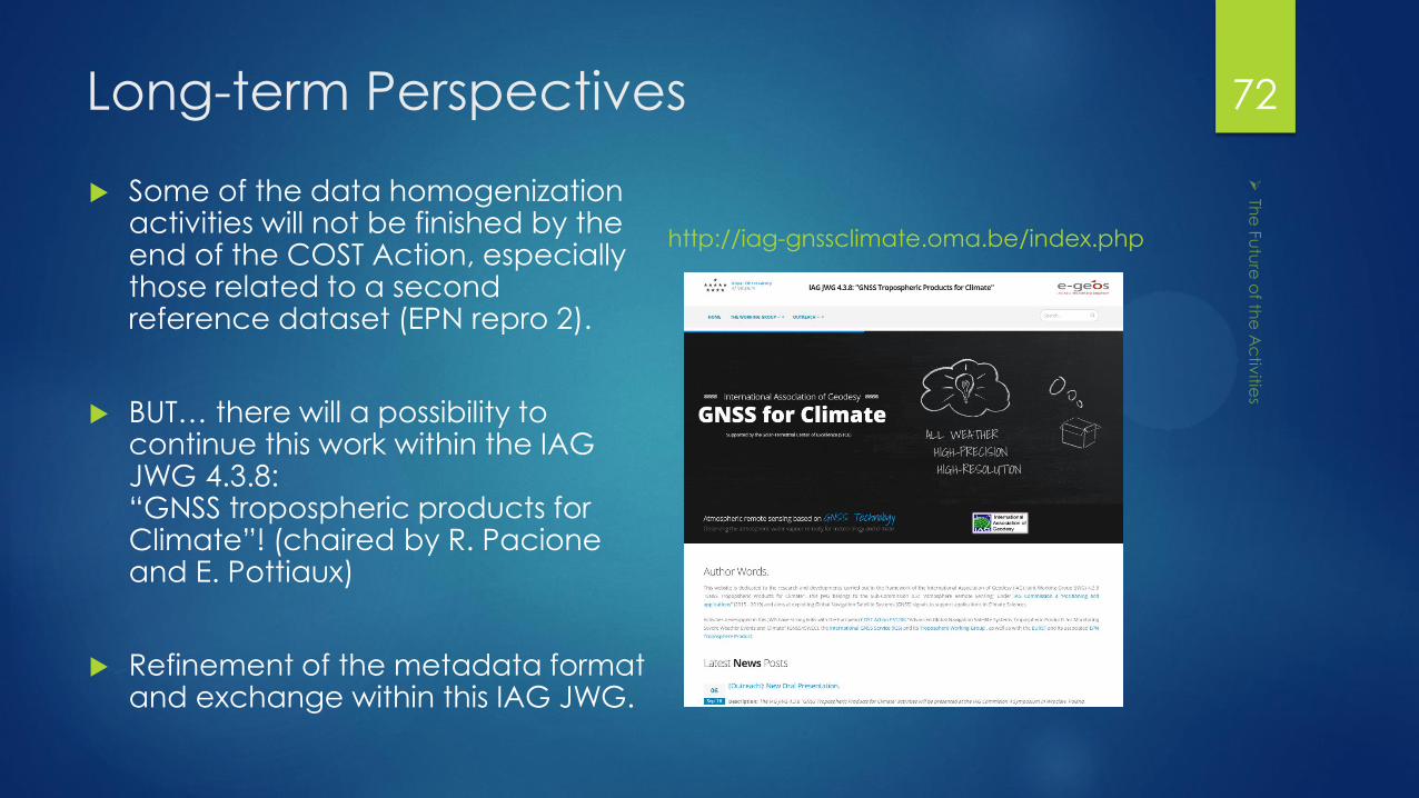
Long-term Perspectives 72

Some of the data homogenization activities will not be finished by the end of the COST Action, especially those related to a second reference dataset (EPN repro 2).

BUT… there will a possibility to continue this work within the IAG JWG 4.3.8: “GNSS tropospheric products for Climate”! (chaired by R. Pacione and E. Pottiaux)

Refinement of the metadata format and exchange within this IAG JWG.

http://iag-gnssclimate.oma.be/index.php

activities of the sub-working group on data...

Documents