ad 42 final 091505 - caltrans - california department of ... 09/15/05 4th issue, final schwarz john...
TRANSCRIPT

..
ILF CONSULTANTS, INC 1440 Broadway, Suite 1010 Telephone: (510) 272 0662 Oakland, CA 94612 Telefax: (510) 272 0647 U.S.A. E-mail: [email protected] Homepage: www.ilf.com
I005/AD-042/FINAL
Devils Slide Tunnel
Geohydrologic Study September 15, 2005
FINAL

D e v i l s S l i d e T u n n e l D e v i l ’ s S l i d e T u n n e l I 0 0 5 / A D - 0 4 2 / F I N A L G e o h y d r o l o g i c S t u d y
I L F C O N S U L T I N G E N G I N E E R S P a g e i ILF/I P:\Devils Slide\Geohydrology Study\ad_42_FINAL_091505.doc
REVISION
3 09/15/05 4th Issue, FINAL Schwarz John Jenkins
2 12/22/2004 3rd Issue, 90% submittal Schwarz John Jenkins
1 11/05/2004 2nd Issue, 65% submittal Schwarz, Gerik
John, Eder
0 10/28/2004 1st Issue Schwarz, Gerik
John, Eder
Rev. Date Issue, Modification Prepared Checked QA/QC

D e v i l s S l i d e T u n n e l D e v i l ’ s S l i d e T u n n e l I 0 0 5 / A D - 0 4 2 / F I N A L G e o h y d r o l o g i c S t u d y
I L F C O N S U L T I N G E N G I N E E R S P a g e ii ILF/I P:\Devils Slide\Geohydrology Study\ad_42_FINAL_091505.doc
TABLE OF CONTENTS
1 INTRODUCTION 1
1.1 Purpose and Scope 1
2 GEOLOGY OF THE PROJECT AREA 1
2.1 Description of Geology 1
2.2 Lithological Units 1
2.3 Type of Aquifer 3
3 DATA BASES 3
3.1 Hydraulic Conductivity K 3
3.2 Hydraulic Heads 5
3.3 Hydrological Data 6
4 ANALYTIC CALCULATIONS 9
4.1 Methodology 9
4.2 Goodman’s Approximation 10
4.3 Asymptotic Solution by Jacob and Lohmann 11
4.4 Cylinder Formula 12
4.5 Herth & Arndts Empiric Approach 12
4.6 General Assumptions 12
5 RESULTS OF THE ANALYTICAL CALCULATIONS 14
5.1 Flush Tunnel Inflow 14

D e v i l s S l i d e T u n n e l D e v i l ’ s S l i d e T u n n e l I 0 0 5 / A D - 0 4 2 / F I N A L G e o h y d r o l o g i c S t u d y
I L F C O N S U L T I N G E N G I N E E R S P a g e iii ILF/I P:\Devils Slide\Geohydrology Study\ad_42_FINAL_091505.doc
5.2 Steady State Tunnel Inflow 15
5.3 Discussion of Results 16
6 NUMERICAL MODELING 17
6.1 Evaluation of the 2001 Geoscience Model 17
6.2 Vertical Models 21
6.3 Model 1 – South Block, km 121+50 22
7 PROPOSED GROUNDWATER INFLOW 26
7.1 Flush Inflow during tunnel excavation 26
7.2 Steady State Groundwater Inflow 27
8 REFERENCES 29
FIGURES Figure 1: Geomorphological Catchment Area for the Devil’s Slide Tunnel Project (red
framed) 8 Figure 2: Early radial inflow (flush inflow) during stage 1 9 Figure 3: Late linear inflow (steady state) during stage 3 10 Figure 4: Position of the numerical models 21
TABLES
Table 1: Localization, Number of Samples, Hydraulic Conductivity (K-Values) and Range of K-Values in orders of magnitude for the individual Lithological and Tectonic Units 4
Table 2: Groundwater Levels applied for Calculations 6 Table 3: Inflow Calculations 14 Table 4: Steady State Inflow Calculations 15 Table 5: Results of the watershed model 18 Table 6: Hydraulic conductivities estimated during the calibration 19 Table 7: Tunnel inflow rates 20

D e v i l s S l i d e T u n n e l D e v i l ’ s S l i d e T u n n e l I 0 0 5 / A D - 0 4 2 / F I N A L G e o h y d r o l o g i c S t u d y
I L F C O N S U L T I N G E N G I N E E R S P a g e iv ILF/I P:\Devils Slide\Geohydrology Study\ad_42_FINAL_091505.doc
APPENDICES
Appendix 1: Groundwater Monitoring Data 31 Appendix 2: Results of the Analytical Tunnel Inflow Calculations 36 Appendix 3: Results of the Numerical Tunnel Inflow Calculations 41 Appendix 4: Tunnel Inflow Calculations by Greg Korbin using Heuer’s Method 51

D e v i l s S l i d e T u n n e l D e v i l ’ s S l i d e T u n n e l I 0 0 5 / A D - 0 4 2 / F I N A L G e o h y d r o l o g i c S t u d y
I L F C O N S U L T I N G E N G I N E E R S P a g e 1 ILF/I P:\Devils Slide\Geohydrology Study\ad_42_FINAL_091505.doc
1 INTRODUCTION
1.1 Purpose and Scope
Groundwater is one of the factors with the highest impact during and after tunnel construction. In order to evaluate (a) the impact of groundwater on tunnel construction and (b) the long and short term impact of tunnel construction on the groundwater system analytical and numerical calculations were conducted. Analytical calculations were applied to (a) estimate flush inflow and (b) steady state inflow for one tunnel bore. In order to calculate the transient inflow and to estimate the influence of the second tube on the groundwater inflow a numeric model was applied.
2 GEOLOGY OF THE PROJECT AREA
2.1 Description of Geology
Two stratigraphic series are expected along the tunnel alignment, namely the Montara granodiorite in the south and Paleocene age sedimentary rocks in the centre and the north. The contact between these two units has been reported to be depositional in some areas and faulted in other areas, but was interpreted in GIR [7] as a fault contact. Montara granodiorite is commonly coarse-grained and may range in composition from quartz diorite to granite, containing pegmatitic veins and hornblende-rich intrusions. The sedimentary rocks include interbedded sandstones, siltstone and claystone as well as conglomerates with individual layers ranging from less than half a meter to perhaps several tens of meters thick. The sedimentary rocks have been extensively folded and faulted. Near the ground surface these rocks are pervasively weathered.
2.2 Lithological Units
Five lithological units are identified along the proposed alignment of the two Devil´s Slide Tunnel bores. The mineralogy, intact rock properties, and discontinuities identified for those units are summarized in EMI documents [4] to [9]. The rock mass description below is a brief compilation of this data.

D e v i l s S l i d e T u n n e l D e v i l ’ s S l i d e T u n n e l I 0 0 5 / A D - 0 4 2 / F I N A L G e o h y d r o l o g i c S t u d y
I L F C O N S U L T I N G E N G I N E E R S P a g e 2 ILF/I P:\Devils Slide\Geohydrology Study\ad_42_FINAL_091505.doc
2.2.1 Granitic Rock
Moderately to very intensely fractured granitic rock. Rock mass is fresh to strongly weathered with partial disintegration of the rock mass. Within the highly fractured rock sections, the appearance of clayey fault gouge is common. Spacing of discontinuities is varying between <3 to 50 cm. The persistence of the discontinuities is in a range of <3 to >6 m.
2.2.2 Claystone
Slightly to intensively fractured claystone. Rock mass is fresh to intensely weathered, in highly fractured and sheared sections, intensely weathered to disintegrated. Spacing of discontinuities is varying between <3 and 40 cm. The persistence is in the range of <3 to >6 m. Highly fractured and sheared sections show soil like rock mass characteristics.
2.2.3 Siltstone
Slightly to intensively fractured siltstone. Rock mass is fresh to intensely weathered, in highly fractured and sheared sections, intensely weathered to disintegrated. Spacing of discontinuities is varying between <3 and 40 cm. The persistence is in a range from <3 to >6 m. Highly fractured and sheared sections show soil like rock mass characteristics.
2.2.4 Sandstone
Slightly to intensively fractured, fine to coarse grained sandstone. The degree of weathering is basically controlled by the intensity of fracturing and varies from fresh to intensely fractured. Spacing of discontinuities is varying between 3 and 40 cm. The persistence is in a range from <3 to 6 m.
2.2.5 Conglomerate
Slightly to intensively fractured, fine to coarse grained conglomerate with transition to coarse grained sandstones. The grain size of the matrix varies from clay to sand. The degree of weathering is controlled by the intensity of fracturing and varies from fresh to intensely fractured. Spacing of discontinuities is varying between 3 and 40 cm. The persistence is in a range from <3 to >6 m.

D e v i l s S l i d e T u n n e l D e v i l ’ s S l i d e T u n n e l I 0 0 5 / A D - 0 4 2 / F I N A L G e o h y d r o l o g i c S t u d y
I L F C O N S U L T I N G E N G I N E E R S P a g e 3 ILF/I P:\Devils Slide\Geohydrology Study\ad_42_FINAL_091505.doc
2.3 Type of Aquifer
2.3.1 Joint Aquifer System
Since the bulk of the rock mass to be expected along the proposed tunnel alignment is bedrock, waterflow is basically taking place along discontinuities (secondary porosity). Therefore it is a function of discontinuity density, aperture and persistence of discontinuities.
2.3.2 Porous Aquifer System
Fault zones, where bedrock is pervasively fractured, constitute soil like rock mass with corresponding hydrogeological properties. Therefore this type of rock mass constitutes a porous aquifer, with a hydraulic conductivity varying from highly permeable (tectonic breccias) to impermeable (fault gouge) depending on the composition of fine grained soils.
3 DATA BASES
3.1 Hydraulic Conductivity K
The values for the hydraulic conductivity K were taken from the well logs and pumping tests as presented in [4], [5] and [11]. ILF has allocated the available data to the lithological units to be encountered along the tunnel alignment. The geological model was obtained from Fig 1-6 of the GIR [9]. The following table shows the K-values of the associated lithological units and their distribution along the tunnel alignment.
D e v i l s S l i d e T u n n e l D e v i l ’ s S l i d e T u n n e l I 0 0 5 / A D - 0 4 2 / F I N A L G e o h y d r o l o g i c S t u d y
I L F C O N S U L T I N G E N G I N E E R S P a g e 4 ILF/I P:\Devils Slide\Geohydrology Study\ad_42_FINAL_091505.doc
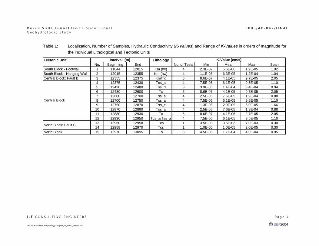
Table 1: Localization, Number of Samples, Hydraulic Conductivity (K-Values) and Range of K-Values in orders of magnitude for the individual Lithological and Tectonic Units
Tectonic Unit LithologyNo. Beginning End No. of Tests Min Mean Max Span
South Block - Footwall 1 11844 12015 Km (fw) 4 2.3E-07 5.6E-06 1.9E-05 1.92South Block - Hanging Wall 2 12015 12355 Km (hw) 4 1.1E-05 6.3E-05 1.2E-04 1.04Central Block: Fault B 3 12355 12375 Km/Tc 5 8.6E-07 4.1E-05 9.7E-05 2.05
4 12375 12430 Tcs_a 4 7.5E-06 6.1E-05 9.5E-05 1.105 12430 12480 Tss_d 3 3.9E-05 1.4E-04 3.4E-04 0.946 12480 12600 Tc 5 8.6E-07 4.1E-05 9.7E-05 2.057 12600 12700 Tss_a 4 2.5E-05 7.6E-05 1.9E-04 0.888 12700 12750 Tcs_a 4 7.5E-06 6.1E-05 9.5E-05 1.109 12750 12870 Tss_c 4 1.3E-06 2.9E-05 6.0E-05 1.6610 12870 12880 Tss_a 4 2.5E-05 7.6E-05 1.9E-04 0.8811 12880 12930 Tc 5 8.6E-07 4.1E-05 9.7E-05 2.0512 12930 12950 Tcs_a/Tss_a 4 7.5E-06 6.1E-05 9.5E-05 1.1013 12950 12958 Tcs 1 3.5E-03 3.5E-03 7.0E-03 0.3014 12958 12970 Tcs 1 1.0E-05 1.0E-05 2.0E-05 0.30
North Block 15 12970 13095 Ts 6 4.5E-05 1.7E-04 4.0E-04 0.95
K-Value [cm/s]Intervall [m]
North Block: Fault C
Central Block

D e v i l s S l i d e T u n n e l D e v i l ’ s S l i d e T u n n e l I 0 0 5 / A D - 0 4 2 / F I N A L G e o h y d r o l o g i c S t u d y
I L F C O N S U L T I N G E N G I N E E R S P a g e 5 ILF/I P:\Devils Slide\Geohydrology Study\ad_42_FINAL_091505.doc
Since values for the hydraulic conductivity K should be regarded as point-specific data, their significance is spatially limited. Even on short distances the K-value may vary over several orders of magnitude for the same lithology. To take this into account, the analytical calculations have been conducted for different K-value to meet these variations:
• The smallest measured value: the inflow calculated with this value has to be expected even under otherwise ideal conditions. The calculated inflow for this value is considered to be the most favorable case.
• The arithmetic mean for all measured values: the arithmetic mean is the sum of all arguments divided by the number of arguments. Its value is always above the ones of the geometric or the harmonic means and it is influenced more strongly by outliers.
• The highest measured value: the calculated inflow for this value is considered to be the most unfavorable case.
It should be kept in mind that the actual variation of the K-value can vary from the available min and max values, as insitu testing can only be carried out randomly. In cases where only single K-value are available, these were assumed to represent the average condition. Instead of a minimum value, the average K-value has been used, while the maximum K-value was assumed to range up to one third of an order of magnitude above the average value.
For the favorable/unfavorable case scenarios, the minimum/maximum water level and the minimum/maximum value for the hydraulic conductivity for the individual sections were applied. The results for average-based calculations were derived using the mean of the water level and the arithmetic mean for the lithology’s hydraulic conductivity.
3.2 Hydraulic Heads
Data regarding hydraulic heads along the tunnel alignment were obtained from the GIR, Fig. 1-6 [9]. These data constitute a snap shot of the groundwater table taken during the soil investigation. Eighteen boreholes have been equipped with piezometers for long term groundwater monitoring. From the available monitoring data [13] it becomes apparent that the annual fluctuation of the groundwater table is small. The standard deviation is, with the exception of BH 02-5B (2.78 m), below 2 m (for most piezometers between 0.5 and 2 m).
The available groundwater monitoring data including hydrographs are summarized in appendix 1. The below table shows minimum and maximum groundwater levels for each of the tectonic and lithological units.

D e v i l s S l i d e T u n n e l D e v i l ’ s S l i d e T u n n e l I 0 0 5 / A D - 0 4 2 / F I N A L G e o h y d r o l o g i c S t u d y
I L F C O N S U L T I N G E N G I N E E R S P a g e 6 ILF/I P:\Devils Slide\Geohydrology Study\ad_42_FINAL_091505.doc
Table 2: Groundwater Levels applied for Calculations (the shown water levels are groundwater levels above the crown)
Tectonic Unit LithologyNo. Beginning End Length Min Max Δh
South Block - Footwall 1 11844 12015 171 Km (fw) 0 10 10South Block - Hanging Wall 2 12015 12355 340 Km (hw) 34 65 31Central Block: Fault B 3 12355 12375 25 Km/Tc 23 34 11
4 12375 12430 50 Tcs_a 20 146 1265 12430 12480 50 Tss_d 102 120 186 12480 12600 120 Tc 82 118 367 12600 12700 100 Tss_a 65 116 518 12700 12750 50 Tcs_a 56 113 579 12750 12870 120 Tss_c 50 109 59
10 12870 12880 10 Tss_a 50 108 5811 12880 12930 20 Tc 42 108 6612 12930 12950 20 Tcs_a/Tss_a 40 107 6713 12950 12958 8 Tcs 18 40 2214 12958 12970 12 Tcs 16 18 2
North Block 15 12970 13095 20 Ts 3 16 13
Tunnel-Water Level [m]Intervall [m]
North Block: Fault C
Central Block
3.3 Hydrological Data
Hydrological data are needed in order to calculate the groundwater recharge rate of the project area. This value, which represents the max. possible steady state tunnel inflow, is used for a plausibility crosscheck of the calculated inflow data. Furthermore hydrological data are essential input for the numerical modeling.
The hydrological data were basically obtained from the Geoscience report [11]. Where possible, other sources were used to check their plausibility. For further analysis Geoscience divided the project area into 4 subareas, estimating values for evapotranspiration, surface runoff and groundwater recharge for each of these subareas. ILF used the mean values of the 4 subareas. Groundwater recharge was calculated by subtracting the evaportranspiration and the surface runoff from the precipitation.
Precipitation
Precipitation data from the San Pedro Valley Park Station of the period between 1989 and 1998 have been used to estimate the mean precipitation of the project area. The period covers wet and dry cycles with a min. value of 501 mm and a max. value of 1515 mm. The mean value of 922 mm is expected to cover the historical average.
Since the San Pedro Valley Park Station is situated 3 km inland of the project site, Geoscience has calculated adjustment factors for the project area. Applying these factors, the annual precipitation in the project area is estimated to range between 700 and 825 mm, depending on the elevation. The derived mean value of 763 mm meets the long term average of the Santa Cruz Station of 758 mm (California Cooperative Snow Surveys [3]).

D e v i l s S l i d e T u n n e l D e v i l ’ s S l i d e T u n n e l I 0 0 5 / A D - 0 4 2 / F I N A L G e o h y d r o l o g i c S t u d y
I L F C O N S U L T I N G E N G I N E E R S P a g e 7 ILF/I P:\Devils Slide\Geohydrology Study\ad_42_FINAL_091505.doc
Evapotranspiration
Geoscience has estimated a potential evapotranspiration rate of 1016 mm (based on information from the NOAA and the mean annual evaporation map in the United States). This corresponds to the information available from the CIMIS (California Irrigation Management Information System) [2], according to which a value of 1003 mm can be estimated (assuming that the project area including the catchment area is situated in evapotranspiration zones 1 to 3).
Based on the potential evapotranspiration an actual transpiration rate with a mean value of 457mm has been calculated.
Surface Runoff
Surface runoff is a function of precipitation, infiltration rate and the slope of an area. Geoscience estimated infiltration rates for the project area based on information provided by the United States Department of Argriculture’s (USDA’s) State Soil Geographic (STATSGO) with a mean value of 5.84 mm/h.
Based on this estimate a surface runoff with an average value of 241 mm was calculated.
Catchment Area
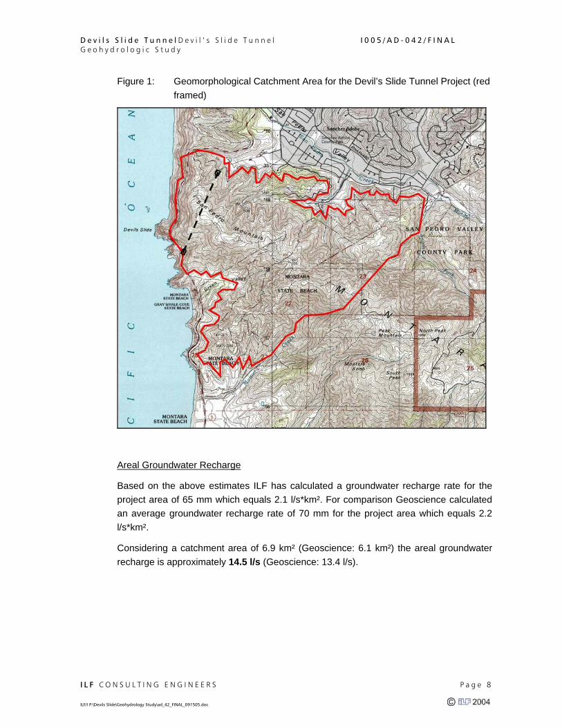
According to the watershed model of Geoscience the catchment area of the Devil’s Slide Tunnel covers 6.1 km². ILF estimated a catchment area of app. 6.9km² considering the following boundaries:
The catchment area roughly forms a triangle (see Figure 1). The north and west boundaries are formed by the 250 feet elevation line running parallel to the Pacific Ocean and the San Pedro Valley. Since the tunnel is situated above 250 feet elevation, groundwater level below this elevation will not be affected by tunnel construction. Furthermore, precipitation falling below this elevation cannot contribute to the tunnel inflow, unless artesic groundwater conditions occur (not assumed on project area scale). The southeastern boundary is formed by the Martini Creek, draining towards the SW into the Pacific Ocean and the South Fork of the San Pedro Creek, draining towards the NW into the Pacific Ocean.
D e v i l s S l i d e T u n n e l D e v i l ’ s S l i d e T u n n e l I 0 0 5 / A D - 0 4 2 / F I N A L G e o h y d r o l o g i c S t u d y
I L F C O N S U L T I N G E N G I N E E R S P a g e 8 ILF/I P:\Devils Slide\Geohydrology Study\ad_42_FINAL_091505.doc
Figure 1: Geomorphological Catchment Area for the Devil’s Slide Tunnel Project (red framed)
Areal Groundwater Recharge
Based on the above estimates ILF has calculated a groundwater recharge rate for the project area of 65 mm which equals 2.1 l/s*km². For comparison Geoscience calculated an average groundwater recharge rate of 70 mm for the project area which equals 2.2 l/s*km².
Considering a catchment area of 6.9 km² (Geoscience: 6.1 km²) the areal groundwater recharge is approximately 14.5 l/s (Geoscience: 13.4 l/s).
D e v i l s S l i d e T u n n e l D e v i l ’ s S l i d e T u n n e l I 0 0 5 / A D - 0 4 2 / F I N A L G e o h y d r o l o g i c S t u d y
I L F C O N S U L T I N G E N G I N E E R S P a g e 9 ILF/I P:\Devils Slide\Geohydrology Study\ad_42_FINAL_091505.doc
4 ANALYTIC CALCULATIONS
4.1 Methodology
In order to predict groundwater inflow into the tunnel analytical calculations were conducted. ILF calculated tunnel inflow using different analytical solutions and included sensitivity analyses for the different tunnel sections. Four different approaches were applied:
• Method by Goodman (1965) • Method by Jacob & Lohmann (1952). • Cylinder formula • Method by Herth & Arndts (1973)
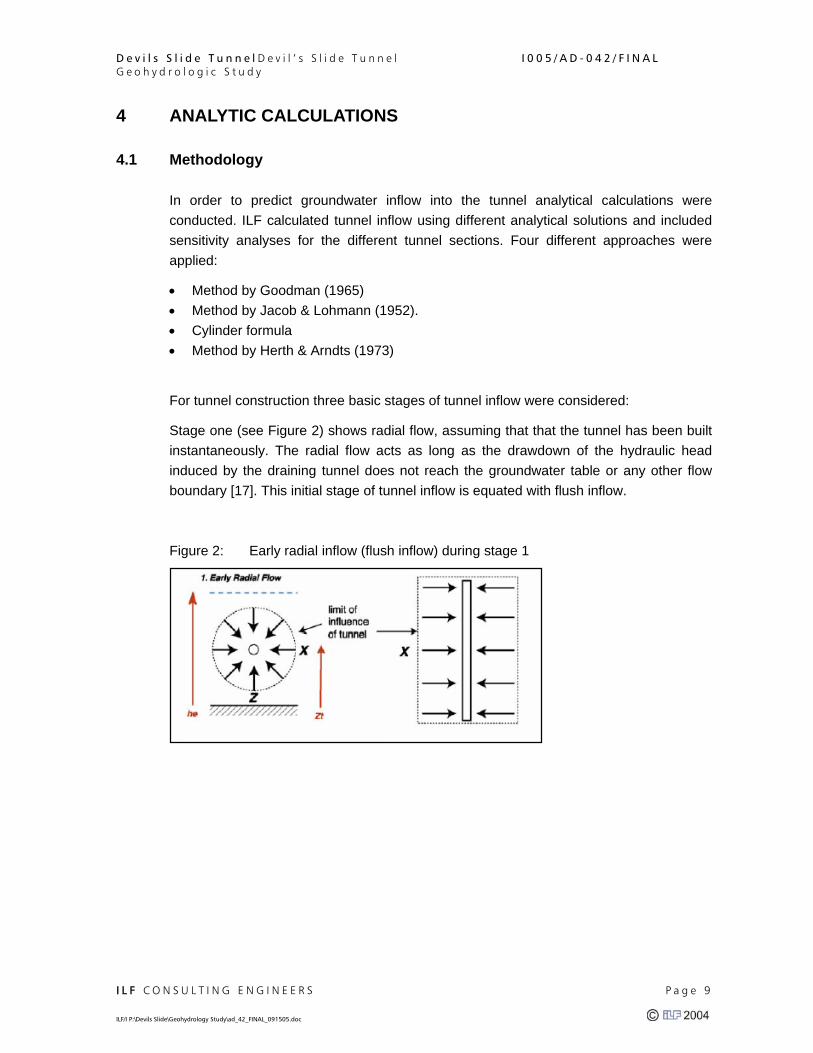
For tunnel construction three basic stages of tunnel inflow were considered:
Stage one (see Figure 2) shows radial flow, assuming that that the tunnel has been built instantaneously. The radial flow acts as long as the drawdown of the hydraulic head induced by the draining tunnel does not reach the groundwater table or any other flow boundary [17]. This initial stage of tunnel inflow is equated with flush inflow.
Figure 2: Early radial inflow (flush inflow) during stage 1

D e v i l s S l i d e T u n n e l D e v i l ’ s S l i d e T u n n e l I 0 0 5 / A D - 0 4 2 / F I N A L G e o h y d r o l o g i c S t u d y
I L F C O N S U L T I N G E N G I N E E R S P a g e 10 ILF/I P:\Devils Slide\Geohydrology Study\ad_42_FINAL_091505.doc
Once the water table drawdown drops to the elevation of the tunnel crown, the inflow can be approximated by purely horizontal flow [17]. This stage of tunnel inflow is equated with steady state inflow.
Figure 3: Late linear inflow (steady state) during stage 3
The transient stage 2 (i.e. between the time when the drawdown cone first affects the groundwater table and the time when the drawdown reaches tunnel elevation) has not been considered in the analytical calculations due to the lack of necessary input data for the analytical calculations. The transient stage has been modeled using numerical modeling.
For calculating the flush inflow the approaches of Goodman [14] and Jacob & Lohmann (in [17]) were used. Steady state inflow was calculated using the cylinder formula (in [18]) and the approach by Herth & Arndts [15].
The calculations were carried out as a parameter study using the minimum, the average and the maximum value of the input data and applying a tunnel radius of 5.6 m.
4.2 Goodman’s Approximation
Polubarinova-Kochina (1962) [19], Goodman (1965) [14], Lei (1999) [16] and El Tani (1999) [12] provide different ways for deriving the same equation of approximating the tunnel inflow for tunnels that are overlain by a constant water column that is much larger than the tunnel’s radius (eq. 1).

D e v i l s S l i d e T u n n e l D e v i l ’ s S l i d e T u n n e l I 0 0 5 / A D - 0 4 2 / F I N A L G e o h y d r o l o g i c S t u d y
I L F C O N S U L T I N G E N G I N E E R S P a g e 11 ILF/I P:\Devils Slide\Geohydrology Study\ad_42_FINAL_091505.doc
The equation itself resembles Thiem’s well formula [20], but it assumes a special geometry with respect to the drawdown.
⎟⎠⎞
⎜⎝⎛ Δ⋅Δ
⋅=
rh
hKQ2ln
2π eq. 1
Q: tunnel inflow [m3 s-1] K: hydraulic conductivity [m/s] Δh: distance between the center of the tunnel and the groundwater table
[m] r: tunnel radius [m]
Goodman’s formula is probably the most commonly used approximation for calculating early tunnel inflow rates. It also serves as the basis of the calculations of the empirical method proposed by Heuer [10].
4.3 Asymptotic Solution by Jacob and Lohmann
A second approach for calculating the first phase radial flow is described by the asymptotic constant head solution of Jacob & Lohmann (1952) (in [17]):
⎟⎠⎞
⎜⎝⎛
⋅⋅⋅⋅
⋅
Δ⋅⋅⋅=
225.2log3.2
4)(
rStLK
hLKtQ π eq. 2
Q: tunnel inflow [m3 s-1] t: point of time [s] K: hydraulic conductivity [m/s] L: length of the tunnel section under construction [m] Δh: distance between the center of the tunnel and the groundwater table
[m] S: elastic storativity r: tunnel radius [m]

D e v i l s S l i d e T u n n e l D e v i l ’ s S l i d e T u n n e l I 0 0 5 / A D - 0 4 2 / F I N A L G e o h y d r o l o g i c S t u d y
I L F C O N S U L T I N G E N G I N E E R S P a g e 12 ILF/I P:\Devils Slide\Geohydrology Study\ad_42_FINAL_091505.doc
4.4 Cylinder Formula
Tunnel inflow can be estimated with a very basic approach by assuming the tunnel to be a perfect cylindrical horizontal drain (eq 3). The inflow has been estimated for the actual tunnel surface with an infinitesimal interface.
KirQ ⋅⋅⋅= π2 eq. 3
Q: tunnel inflow [m3 s-1] i: hydraulic gradient [-] K: hydraulic conductivity [m/s] r: tunnel radius [m]
For solid rock with a low hydraulic conductivity K, the gradient i is usually assumed to be i=1. This of course is a strong simplification, since the hydraulic gradient changes significantly along the drawdown’s surface. While the gradient is steep and therefore i>>1 close to the tunnel itself, it’s declining towards the effective radius of the drawdown. For most of the surface of the drawdown, the gradient is i<<1.
4.5 Herth & Arndts Empiric Approach
Another approach for calculating late linear flow of the steady state is the empirical formula by Herth & Arndts (1973) [15] as stated in eq. 4.
( )21
22
22
1227,073,0 hhrK
hhhQ −⋅⋅⎟⎟⎠
⎞⎜⎜⎝
⎛ −⋅+= eq. 4
Q: tunnel inflow [m3 s-1] K: hydraulic conductivity [m/s] h1: hydraulic head for the proximate observation point with respect to the
tunnel center [m] h2: hydraulic head for the remote observation point with respect to the
tunnel center [m] r2: distance from the tunnel center to the remote observation point [m]
4.6 General Assumptions
All of the analytical solutions for the tunnel inflow describe the hydraulic conductivity as a function of the depression cone’s geometry.
El Tani [12] suggests that the drainage area for a tunnel section without major fluctuations of the groundwater table can be assumed to be four times as wide as the
D e v i l s S l i d e T u n n e l D e v i l ’ s S l i d e T u n n e l I 0 0 5 / A D - 0 4 2 / F I N A L G e o h y d r o l o g i c S t u d y
I L F C O N S U L T I N G E N G I N E E R S P a g e 13 ILF/I P:\Devils Slide\Geohydrology Study\ad_42_FINAL_091505.doc
groundwater head measures vertically. The results for the calculations according to Goodman are based on this assumption.
Similar assumptions are implied for most of the analytical solutions. Assumptions for the interrelationship of the depression cone and its effective radius had to be made only for the application of Herth & Arndt’s approach. As the available data does not cover site-specific data from corresponding pumping tests, values were back-calculated from the results of Geoscience’s study [11].

D e v i l s S l i d e T u n n e l D e v i l ’ s S l i d e T u n n e l I 0 0 5 / A D - 0 4 2 / F I N A L G e o h y d r o l o g i c S t u d y
I L F C O N S U L T I N G E N G I N E E R S P a g e 14 ILF/I P:\Devils Slide\Geohydrology Study\ad_42_FINAL_091505.doc
5 RESULTS OF THE ANALYTICAL CALCULATIONS
5.1 Flush Tunnel Inflow
Table 3: Inflow Calculations for One Tube
ILF Heuer 1995Tectonic Unit
No. Length Fav. Av. Unfav. Fav. Av. Unfav. Fav. Av. Unfav. Fav. Av. Unfav.South Block - Footwall Block 1 171 0,30 0,94 0,36 0,00 0,30 0,65South Block - Hanging Wall Block 2 340 0,94 6,85 15,59 0,66 7,28 20,57 0,80 7,07 18,08Central Block: Fault B 3 25 0,06 3,17 8,30 0,02 1,98 6,29 0,04 2,57 7,30
4 50 0,48 11,01 22,02 0,21 9,09 26,35 0,34 10,05 24,185 50 6,97 27,13 68,25 6,13 8,81 85,13 6,55 17,97 76,696 120 0,13 7,22 19,22 0,08 6,35 21,84 0,10 6,78 20,537 100 3,25 12,35 37,19 2,37 11,40 41,92 2,81 11,88 39,558 50 0,88 11,15 18,22 0,58 9,25 20,39 0,73 10,20 19,319 120 0,14 4,31 11,22 0,07 3,39 10,59 0,11 3,85 10,9110 10 2,72 11,22 35,30 1,82 5,34 39,03 2,27 8,28 37,1611 50 0,08 5,89 18,02 0,04 5,16 19,80 0,06 5,52 18,9112 20 0,71 10,11 17,51 0,41 4,38 7,22 0,56 7,24 12,3713 8 212,73 272,81 660,00 180,37 180,37 427,00 196,55 226,59 543,5014 12 0,58 0,59 1,21 0,23 0,23 0,49 0,40 0,41 0,85
North Block 15 125 3,17 8,17 23,07 0,31 3,44 11,67 1,74 5,80 17,37
Goodmann, 1965 Jacob & Lohman 1952
Central Block
North Block: Fault C
Intervall
5,0
9,51,22 8,31 26,02
30,4
Q for 100m tunnel progress [l/s]
5,0
8,5
18,012,38 17,54 45,03
Arith. Av. Weighted Av.
0,53 4,80 12,25
Legend:
Fav.: Favorable Scenario, using min. values of hydraulic conductivity and hydraulic heads within the considered tunnel section
Av.: Average Scenario, mean values of hydraulic conductivity and hydraulic heads within the considered tunnel section
Unfav.: Unfavorable Scenario, max. values of hydraulic conductivity and hydraulic heads within the considered tunnel section

D e v i l s S l i d e T u n n e l D e v i l ’ s S l i d e T u n n e l I 0 0 5 / A D - 0 4 2 / F I N A L G e o h y d r o l o g i c S t u d y
I L F C O N S U L T I N G E N G I N E E R S P a g e 15 ILF/I P:\Devils Slide\Geohydrology Study\ad_42_FINAL_091505.doc
5.2 Steady State Tunnel Inflow
Table 4: Steady State Inflow Calculations for One Tube
ILF Heuer 1995Tectonic Unit
No. Length Fav. Av. Unfav. Fav. Av. Unfav. Fav. Av. Unfav. Fav. Av. Unfav.South Block - Footwall Block 1 171 0,01 0,34 1,14 0,05 0,32South Block - Hanging Wall Block 2 340 1,32 7,57 14,36 1,27 10,65 26,53Central Block: Fault B 3 25 0,01 0,36 0,85 0,00 0,16 0,44
4 50 0,13 1,26 1,67 0,06 2,18 5,085 50 0,69 2,52 5,98 2,00 7,94 20,416 120 0,04 1,73 4,10 0,06 3,29 9,167 100 0,88 2,66 6,69 1,63 4,56 14,698 50 0,13 1,26 1,67 0,14 3,02 5,369 120 0,05 1,22 2,53 0,08 2,75 7,8510 10 0,09 0,27 0,67 0,13 0,60 2,0511 50 0,02 0,72 1,71 0,01 1,03 3,4912 20 0,05 0,50 0,67 0,04 0,70 1,3513 8 3,36 5,41 14,9014 12 0,01 0,01 0,03
North Block 15 125 0,15 1,38 5,33Sum 8,92 43,72 117,00 16 43,6
IntervallCylinder Formula
1,33 7,91 15,50
North Block: Fault C
Central Block 2,09 12,50 26,53
8,8
6 24,0
1,27 10,70 26,85
4,13 26,22 69,89
7 10,8
Herth & Arendts 1973Q for tunnel section [l/s]
NOT APPLICABLE
incl. Safety Factor of 2
3,52 6,81 20,26
3
Legend:
Fav.: Favorable Scenario, using min. values of hydraulic conductivity and hydraulic heads within the considered tunnel section
Av.: Average Scenario, mean values of hydraulic conductivity and hydraulic heads within the considered tunnel section
Unfav.: Unfavorable Scenario, max. values of hydraulic conductivity and hydraulic heads within the considered tunnel section

D e v i l s S l i d e T u n n e l D e v i l ’ s S l i d e T u n n e l I 0 0 5 / A D - 0 4 2 / F I N A L G e o h y d r o l o g i c S t u d y
I L F C O N S U L T I N G E N G I N E E R S P a g e 16 ILF/I P:\Devils Slide\Geohydrology Study\ad_42_FINAL_091505.doc
5.3 Discussion of Results
5.3.1 General Comments
The results of the analytical calculations produced by ILF were compared with the results of the analytical calculations using Heuers approach (see Appendix 4), carried out independently by Greg Korbin [10]. It has to be mentioned that the results represent tunnel inflow for one tube only. The results of this comparison are provided below.
5.3.2 Flush Tunnel Inflow
Table 3 summarizes the results of the calculations of flush tunnel inflow for 100 m long tunnel sections. To compare ILF results with the results of the Heuer method, ILF calculated the arithmetic mean of the results according to Goodman and Jacob & Lohman for each lithological unit (average values). In a second step the results were summarized for each of the three tunnel sections by calculating the weighted average. These average results are generally in accordance with the results provided by the Heuer method.
Only the calculated tunnel inflow for the North Block is app. 2/3 of the value according to Heuer. This deviation is due to the fact that the Heuer approach does not weight the influence of the length of the tunnel section in the same way this is done by calculating the weighted average. The impact of the tunnel length increases with the increase of the variation of the K-values. It was found that tunnel length has little impact on the results in the South and Central Block since the K-values show only minor variations compared to the setting in the North Block. Here the variation of K-values is high due to the occurrence of the highly permeable zone along fault C.
Choosing 100 m length has been found to be unreasonable for calculating flush tunnel inflow since, especially in highly permeable zones such as fault zones, this approach results in unrealistic high values of several 100 l/s. The extent of fault zones in the project area is limited to few meters. Hence, such high values are will not be encountered during actual tunneling. This fact should be considered when reviewing the results shown in Table 3.
5.3.3 Steady State Tunnel Inflow
The applied numerical calculations are simple solutions for calculating both flush and steady state groundwater inflow into tunnels. However all those methods are based on assumptions which have to be considered assessing the results.
The analytical methods generally assume that the groundwater body is laterally unconfined. In contrary the groundwater’s body at the Devil’s Slide Tunnel Project area is

D e v i l s S l i d e T u n n e l D e v i l ’ s S l i d e T u n n e l I 0 0 5 / A D - 0 4 2 / F I N A L G e o h y d r o l o g i c S t u d y
I L F C O N S U L T I N G E N G I N E E R S P a g e 17 ILF/I P:\Devils Slide\Geohydrology Study\ad_42_FINAL_091505.doc
laterally confined due to the triangular shape of the geomorphological catchment area (see Figure 1). Based on the current standard of knowledge it is believed that the hydrogeological catchment area does not exceed the morphological catchment area. Assuming a catchment area of 6.9 km², an average groundwater recharge ratio of 14.5 l/s can be expected (see Chapter 3.3). This value can be understood as a maximum value for steady state tunnel inflow (the assumption is on the safe side since it implies that all groundwater recharge drains towards the tunnel). Therefore ILF proposes to use the average of the calculated “Favorable Values” (see Table 4) for average steady state tunnel inflow prediction to one tunnel tube, applying an uncertainty factor of two. This factor of safety is found reasonable due to uncertainties in connection with groundwater inflow along fault zones and the occurrence of unknown highly permeable zones. The results show a total discharge for one tunnel tube of 16 l/s.
Due to experiences it is not reasonable to double the proposed inflow value in order to consider the second tunnel tube. In fact numerous tunneling projects have shown that the groundwater inflow increases by the factor of 20% due to the second tube ([10] and [17]). This would result in a steady state inflow of app. 20 l/s for both tunnels. In order to consider the fluctuation of the annual precipitation ratio (dry and wet years) a supplement of 50 % is added, leading to a final figure for steady state inflow of 30 l/s.
6 NUMERICAL MODELING
6.1 Evaluation of the 2001 Geoscience Model
6.1.1 Overview
The model is generated and calibrated based on the findings in Woodward-Clyde (1996) [4].
The more recent data provided by EMI ([5] to [9]) have improved and changed the understanding of the geological structure as well as the spatial distribution of the hydraulic heads. The new findings with respect to the general ground water flow direction or the impact of faults (e.g. fault C and fault 02-5) are not represented within the 2001 numeric model.
Numerical modeling was carried out in order to determine tunnel inflow for the second tube.
6.1.2 Watershed Model
Four subareas are accounted for and named Eastern, Southern, Western and Northern Subarea. For the precipitation, meteorological data from the station at San Pedro Valley Park between 1989 and 1998 is used and fitted to the model area’s morphology by

D e v i l s S l i d e T u n n e l D e v i l ’ s S l i d e T u n n e l I 0 0 5 / A D - 0 4 2 / F I N A L G e o h y d r o l o g i c S t u d y
I L F C O N S U L T I N G E N G I N E E R S P a g e 18 ILF/I P:\Devils Slide\Geohydrology Study\ad_42_FINAL_091505.doc
calculating an adjustment factor from the isohyetal map. In addition, the potential evapotranspiration is calculated. Estimates of the infiltration rate of soil in each subarea are derived from the United States Department of Agriculture’s State Soil Geographic database.
The hydrologic budget for the subareas is computed using the program ‘Hydrological Simulation Program – Fortran’ (HSPF; Bicknelli et al. 1997 [1]). It uses the given precipitation and potential evapotranspiration to estimate surface runoff, evapotranspiration and ground water recharge within the watershed as shown in Table 5.
Table 5: Results of the watershed model
Eastern Southern Western Northern Adjustment Factor 0.89 0.83 0.76 0.81 Calculated Precipitation [mm/a] 821 765 701 747 Surface Runoff [mm/a] 279 254 203 229 Evapotranspiration [mm/a] 483 457 431 457 Ground Water Recharge [mm/a] 76 76 51 76 Mass balance error [%] 2.1% 2.9% -2.3% 2.0% Infiltration Rate [mm/h] 5.84 8.13 6.35 4.83
6.1.3 Numeric Model
6.1.3.1 Boundary Conditions
For the Southern, Western and Northern model boundaries, boundary conditions of the first kind (= Dirichlet boundary condition) are applied. Neither piezometric heights nor mass transfer rates for the calculated in-/outflow are documented in the Geoscience report.
For the Eastern model boundary, a boundary condition of the second kind (= Neumann boundary condition) is applied. The inflow rate is assumed to be 4,600 m³/d (843 gpm). It is reported in the Geoscience Report to act similar to a boundary condition of first kind, but again, no piezometric elevation is mentioned.
The tunnel sections are considered as drains with an initial drain capacity of 77% of their final conductance. The Geoscience Report does not mentioned at what point in time the total drain capacity is applied.
6.1.3.2 Parameterization
The model generation and manipulation is performed using the MODFLOW-based software packages Ground Water Vistas 3.0 and GMS 3.1.
The finite-difference model’s grid covers an area of approximately 6 km² and consists of 267,150 cells (137x195 cells in 10 layers), 117,357 of which are considered to be active
D e v i l s S l i d e T u n n e l D e v i l ’ s S l i d e T u n n e l I 0 0 5 / A D - 0 4 2 / F I N A L G e o h y d r o l o g i c S t u d y
I L F C O N S U L T I N G E N G I N E E R S P a g e 19 ILF/I P:\Devils Slide\Geohydrology Study\ad_42_FINAL_091505.doc
during the computations. Each model cell is approximately a cube, measuring 15 m on a side.
The hydraulic conductivities in Y-direction for the different lithological units are estimated during the calibration by PEST (calibration module of MODFLOW). The values for the hydraulic conductivities in X-direction are lower than the ones in Y-direction by a factor of 5 with respect to the steep gradient.
The hydraulic conductivity in vertical direction is assumed to be 0.02 m/d (2.5E-05 cm/s) independent from the lithological units, including the faults. This assumption is not sustained and it does not correspond with the standard interpretation of the material properties, which would suggest to assume igneous rocks to behave almost isotropic, sedimentary rocks being less permeable in the bedding direction by an order of one magnitude and open faults being highly permeable in their direction of strike and normal to their dip direction, but showing a low permeability in their dip direction.
The storativity is assumed to be independent from the lithological units as well and to be a decreasing function of the depth instead.
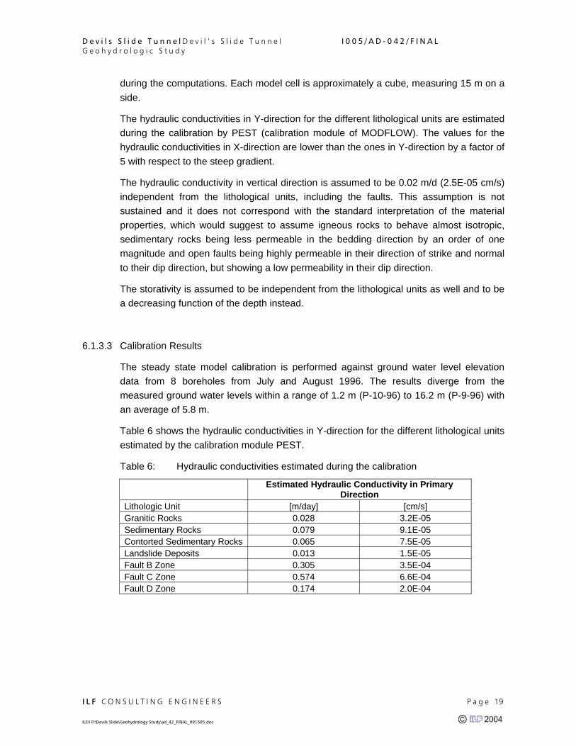
6.1.3.3 Calibration Results
The steady state model calibration is performed against ground water level elevation data from 8 boreholes from July and August 1996. The results diverge from the measured ground water levels within a range of 1.2 m (P-10-96) to 16.2 m (P-9-96) with an average of 5.8 m.
Table 6 shows the hydraulic conductivities in Y-direction for the different lithological units estimated by the calibration module PEST.
Table 6: Hydraulic conductivities estimated during the calibration
Estimated Hydraulic Conductivity in Primary
Direction Lithologic Unit [m/day] [cm/s] Granitic Rocks 0.028 3.2E-05 Sedimentary Rocks 0.079 9.1E-05 Contorted Sedimentary Rocks 0.065 7.5E-05 Landslide Deposits 0.013 1.5E-05 Fault B Zone 0.305 3.5E-04 Fault C Zone 0.574 6.6E-04 Fault D Zone 0.174 2.0E-04

D e v i l s S l i d e T u n n e l D e v i l ’ s S l i d e T u n n e l I 0 0 5 / A D - 0 4 2 / F I N A L G e o h y d r o l o g i c S t u d y
I L F C O N S U L T I N G E N G I N E E R S P a g e 20 ILF/I P:\Devils Slide\Geohydrology Study\ad_42_FINAL_091505.doc
6.1.3.4 Results
The actual model is computed for three different stages: the construction phase, the finalization of the construction after 1.6 years and a near-equilibrium stage 5 years after the construction was completed. Two scenarios are applied:
• Scenario 1 – Average Conditions. An areal recharge of 50-70 mm/a is applied along with values for the effective porosity of 0.02-0.1 and for the storativity of 0.0001-0.02.
• Scenario 2 – Unfavorable Conditions. The values of storativity and effective porosity are increased to account for the uncertainty of these parameters to ranges between 0.0005-0.05 respectively 0.05-0.12. The values for the recharge under wet year conditions are doubled. These assumptions are not sustained by calculations.
For either scenario, the hydraulic head above the tunnel at the end of the tunneling process is predicted to be less than 5 m along the entire tunnel and within 1 m for most of the tunnel. Further predictions include that the hydraulic heads will have lowered to within 2 m of the tunnel elevation along the entire tunnel alignment by five years after the end of construction. The suggested tunnel inflow rates are shown in Table 7.
Table 7: Tunnel inflow rates (for both tunnel tubes)
Scenario 1 Scenario 2 [gpm] [l/s] [gpm
] [l/s]
Total Tunnel Inflow during Construction 339 21.4 495 31.2 Total Tunnel Inflow after Completion 119 7.5 183 11.5 Total Tunnel Inflow at Near-Equilibrium 55 3.5 101 6.4
6.1.4 Recommendations
Geoscience already recommended that the monitoring of the existing boreholes and additional ground water levels in new borings are collected on a regular basis to improve the understanding of the regional ground water table’s behavior and establish baseline conditions before the start of construction. These recommendations include also collecting data from monitoring any streamflow or spring in the model area.
During tunneling, it is recommended that all established piezometers, drainages and springs are continuously monitored in order to asses the effects that the tunneling may have on the ground water discharge.

D e v i l s S l i d e T u n n e l D e v i l ’ s S l i d e T u n n e l I 0 0 5 / A D - 0 4 2 / F I N A L G e o h y d r o l o g i c S t u d y
I L F C O N S U L T I N G E N G I N E E R S P a g e 21 ILF/I P:\Devils Slide\Geohydrology Study\ad_42_FINAL_091505.doc
6.2 Vertical Models
6.2.1 General
Three vertical models situated at different hydrological units have been generated for the estimation of groundwater table – drawdown and inflow to both tunnel tubes. The models are orientated rectangular or nearly rectangular to tunnel axis, groundwater flow will be forced to this direction by the drainage effect of the tunnels (see figure 0-1 in Appendix 3).
Figure 4: Position of the numerical models
The vertical models are simulated as a slice of 1 m thickness. The results can therefore be regarded as inflow for a 1 m long tunnel section. Tunnel inflow for the entire tunnellength is obtained by interpolating and extrapolating these results.
Finite-Element-Technology (FE) based on the software “Feflow” (developed by Wasy-Berlin) was used for modeling. Each model consists of approximately 5000 triangular elements. FE allows a good fit to curved and polylined boundaries like tunnel sections, topography or faults. The baseline of the models was set to a level of –60 m.
The tunnels were simulated by setting the conductivity of the elements within the tunnel boundary to a value of 100 m/s and integrating a constant head boundary at a level close to the tunnel invert. Using this method no numerical instabilities due to internal holes occurred.
Model 1
Model 2
Model 3

D e v i l s S l i d e T u n n e l D e v i l ’ s S l i d e T u n n e l I 0 0 5 / A D - 0 4 2 / F I N A L G e o h y d r o l o g i c S t u d y
I L F C O N S U L T I N G E N G I N E E R S P a g e 22 ILF/I P:\Devils Slide\Geohydrology Study\ad_42_FINAL_091505.doc
First a steady-state calculation for simulating the undisturbed situation (before tunnel excavation) was performed. The calibration of conductivity and groundwater recharge showed that the existing groundwater table could only be simulated by applying low conductivity values (lower bound values) and a groundwater recharge of 150 mm/year (upper bound value).
Using the calibrated models a transient calculation was performed including the following time steps and boundary conditions:
Time step 0: Start of NB-Tunnel excavation Period 0 – 30 days: 300 steps with length 0.1 d each Time step 30 days: Start of SB-Tunnel excavation Period 30 – 400 days: 370 steps with length 1 d each
Note that the following stations refer to stationing of the NB tunnel.
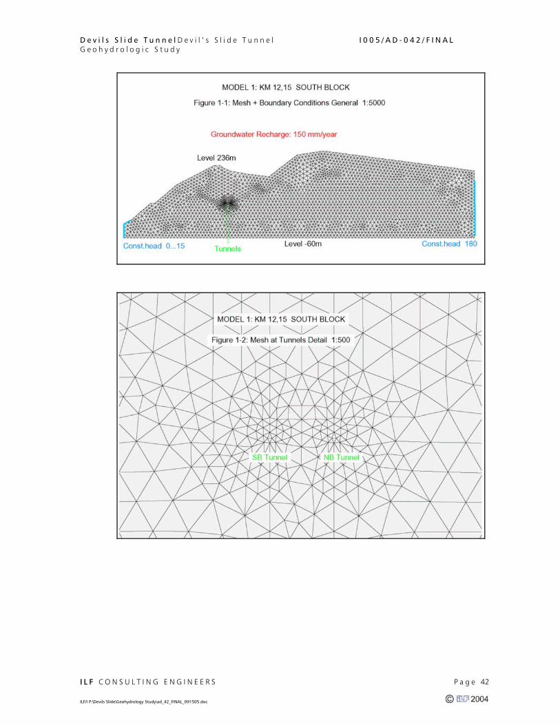
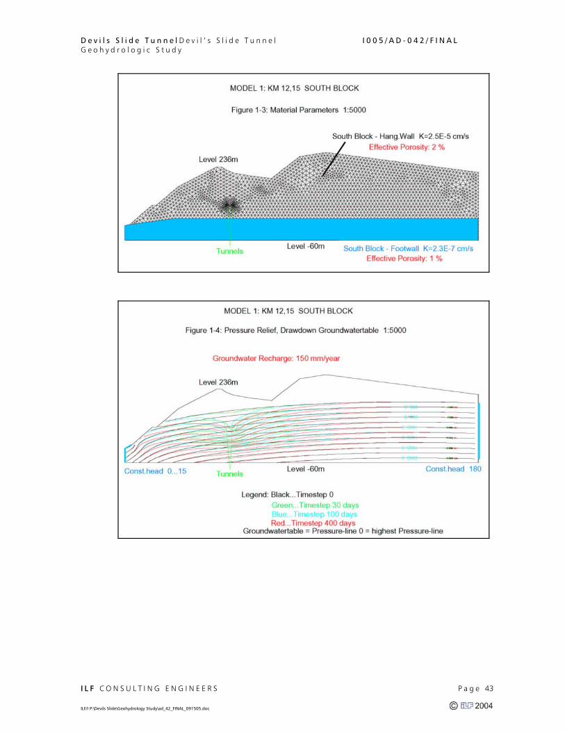
6.3 Model 1 – South Block, km 121+50
Ref.: Figures 1-1 to 1-6 in Appendix 3.
6.3.1.1 Geometry
The model is situated at km 121+50 in the South Block, with a groundwater table of 150 m above sea level. The orientation of the model is perpendicular to the tunnel axis. The model extends from the shoreline 1415 m to the east. The two tunnels are situated 405 respectively 431 m to the east of the shoreline.
6.3.1.2 Boundary Conditions
Left side (shore): Constant head level is 0 to 15 m
The condition was chosen for simulating groundwater outflow of the hanging wall layer with higher conductivity, indicated by springs close to the shoreline in the vicinity of fault A (see Figure 4).
Right Side: Constant head level is 180 m
This level corresponds to results of the 2001 Geoscience model. The flow direction at this boundary is towards the east and it can be assumed that the groundwater table will not to be affected by the tunnel over this distance.

D e v i l s S l i d e T u n n e l D e v i l ’ s S l i d e T u n n e l I 0 0 5 / A D - 0 4 2 / F I N A L G e o h y d r o l o g i c S t u d y
I L F C O N S U L T I N G E N G I N E E R S P a g e 23 ILF/I P:\Devils Slide\Geohydrology Study\ad_42_FINAL_091505.doc
6.3.1.3 Material Parameters
South Block Footwall: K = 2.3E-7 cm/s, Porosity: 1%
South Block Hanging Wall: K = 2.5E-5 cm/s, Porosity: 2%
The two blocks are separated by Fault A which extents between level 0 to 30 m (see Appendix 3 Figure 1-3).
During the calibration process the K-value of the hanging wall formation was varied between 1.1 and 6.3 E-5 cm/s. At a K-value of 2.5 E-5 cm/s the groundwater table showed good coincidence.
6.3.1.4 Results
Drawdown of the Groundwater Table
Figure 1-4 in Appendix 3 shows the groundwater table at time steps 0, 30, 100 and 400 days. After 30 days groundwater drawdown is as much as approx. 8 m, while after 100 days drawdown has reached tunnel level (= 79 m above sea level). The level of undisturbed groundwater table is 150 m above sea level, the magnitude of drawdown 71 m.
Tunnelinflow
Tunnelinflow is shown on Figure 1-6 (Appendix 3). The hydrograph of the inflow to the NB tunnel shows an initial inflow of 13.2 m³/d*m followed by a rapid decrease of the inflow rate to approx. 2.7 m³/d*m after 30 days. After the start of the excavation of SB-Tunnel (timestep 30 days) an initial inflow of 6.6 m³/d*m to the SB tunnel occurs (total tunnel inflow of 8.9 m³/d*m), also followed by a rapid decrease. After 400 days the total inflow reaches 1 m³/d*m, 1/3 from the SB-Tunnel and 2/3 from the NB-Tunnel.
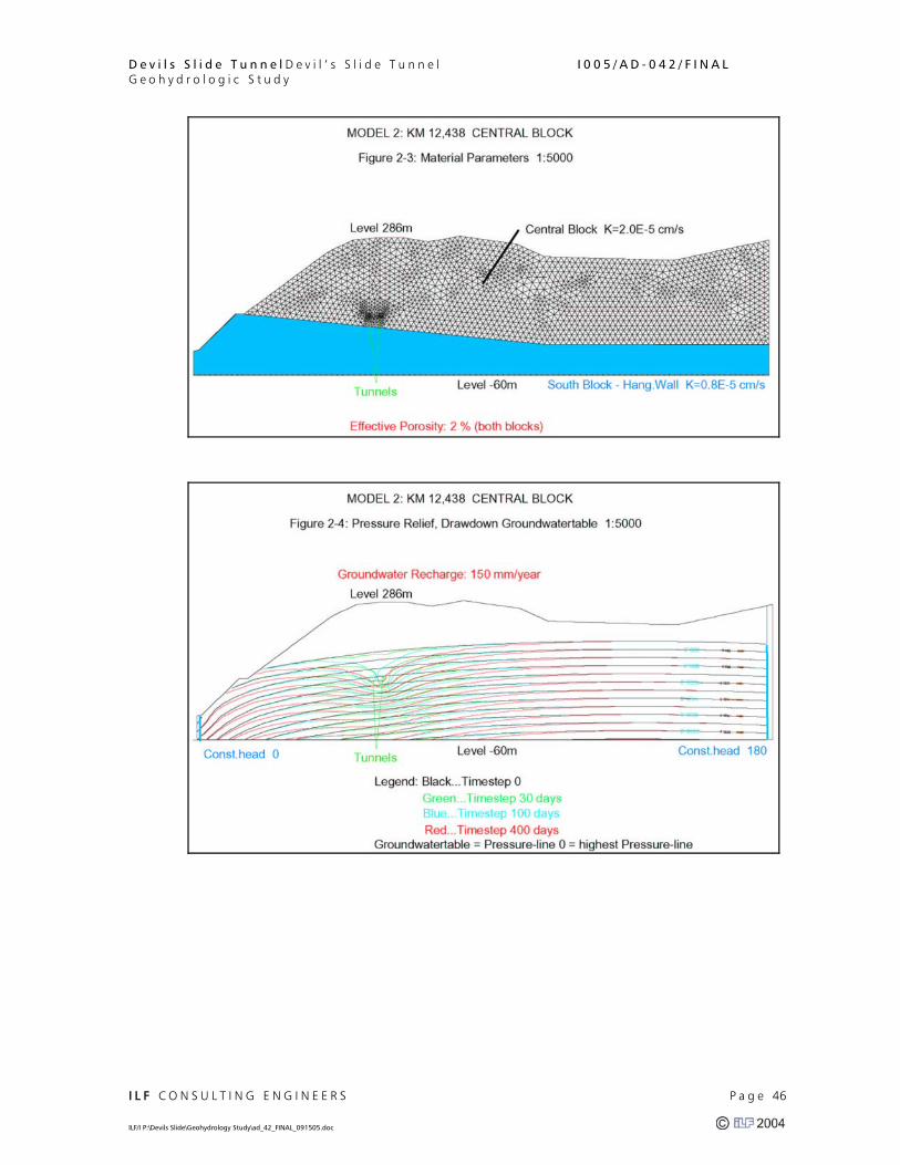
6.3.2 Model 2 – Central Block, km 124+38
Ref.: Figures 2-1 to 2-6 in Appendix 3
6.3.2.1 Geometry
The model is situated at km 124+38 close the southern boundary of the Central Block at the location of the higher groundwater table (157 m). The orientation of the model is parallel to the sub vertical fault zone 02-5 (= 8° to north and 79° to tunnel axis) and perpendicular to tunnel axis (see Figure 4). The model extends from shoreline 1450 m to

D e v i l s S l i d e T u n n e l D e v i l ’ s S l i d e T u n n e l I 0 0 5 / A D - 0 4 2 / F I N A L G e o h y d r o l o g i c S t u d y
I L F C O N S U L T I N G E N G I N E E R S P a g e 24 ILF/I P:\Devils Slide\Geohydrology Study\ad_42_FINAL_091505.doc
the east. The two tunnels are situated 442 respectively 471 m to the east of the shoreline.
6.3.2.2 Boundary Conditions
Left side (shoreline): Constant head level 0 m
Right side: Constant head level 180 m
This level corresponds to results of the 2001 Geoscience model. The flow direction at this boundary is towards the east and it can be assumed that the groundwater table will not to be affected by the tunnel over this distance.
6.3.2.3 Material Parameters
South Block Hanging Wall: K = 0.8E-5 cm/s; Porosity: 2 %
Central Block: K = 2.0E-5 cm/s; Porosity: 2 %
The two blocks are separated by Fault B which extents between level 15 and 90 m, the tunnels are located at a level of 60 m, see Figure 2-3 (Appendix 3).
A groundwater table of 160 m was achieved by using relatively small K-values.
6.3.2.4 Results
Drawdown of the Groundwater Table
Figure 2-4 in Appendix 3 shows the groundwater table at time steps 0, 30, 100 and 400 days. After 30 days groundwater drawdown is approx. 8m, after 100 days approx. 50 m, while after 200 days drawdown has reached tunnel level (=84 m above sea level). The level of undisturbed groundwater table is 157 m above sea level, the magnitude of drawdown 73m.
Tunnelinflow
Figure 2-6 in Appendix 3 shows the hydrographs of the inflow to the NB and SB tunnel as well as the sum of both. The hydrograph for the NB tunnel shows an initial inflow of 13.5 m³/d*m followed by a rapid decrease to 2.4 m³/d*m after 30 days. The initial inflow to the SB tunnel (time step 30 days) reaches 6.8 m³/d*m, also followed by a rapid decrease. After 400 days the total inflow reaches 1 m³/dm, 1/3 from the SB-Tunnel and 2/3 from the NB-Tunnel.

D e v i l s S l i d e T u n n e l D e v i l ’ s S l i d e T u n n e l I 0 0 5 / A D - 0 4 2 / F I N A L G e o h y d r o l o g i c S t u d y
I L F C O N S U L T I N G E N G I N E E R S P a g e 25 ILF/I P:\Devils Slide\Geohydrology Study\ad_42_FINAL_091505.doc
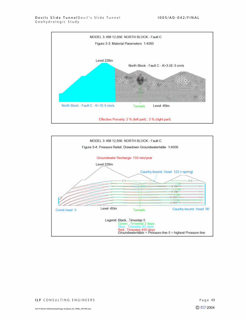
6.3.3 Model 3 – North Block Fault C, km 129+56
Ref.: Figures 3-1 to 3-6 in Appendix 3.
6.3.3.1 Geometry
Model 3 is situated at km 129+56 within the high permeable zone of Fault C at the southern boundary of the north block. The orientation is almost parallel to Fault C (= 78.5° to tunnel axis). The model extends from the shoreline 1079 m to the east. The tunnels are situated 585 respectively 614 m east of the shoreline.
6.3.3.2 Boundary Conditions
Left side (shore): Constant head level 0 m.
Right side: Cauchy-boundary condition level 90 m
Spring 100 m east of tunnel: Cauchy-boundary condition level 122 m
With the help of the Cauchy boundary condition (setting inflow transfer rate to 0) physically incorrect inflow into model can be avoided during groundwater drawdown.
Concentration of Groundwater Recharge
The calibration of the model resulted in much higher inflow rates (factor 10) than a recharge of 150 mm would provide. This can be explained by the draining effect of the permeable Fault C zone, which dewaters the adjacent northern part of the Central Block with its higher groundwater table.
6.3.3.3 Material Parameters
North Block Fault C: see Figure 3-3 in Appendix 3
Central and right profile section (area of fault C): K = 3.5 E-3cm/s
Left profile section (relatively undisturbed rock mass): K = 1E-5 cm/s
For the left profile section the lower k-value was applied in order to raise the groundwater table to 123 m.
6.3.3.4 Results
Drawdown of the Groundwater Table

D e v i l s S l i d e T u n n e l D e v i l ’ s S l i d e T u n n e l I 0 0 5 / A D - 0 4 2 / F I N A L G e o h y d r o l o g i c S t u d y
I L F C O N S U L T I N G E N G I N E E R S P a g e 26 ILF/I P:\Devils Slide\Geohydrology Study\ad_42_FINAL_091505.doc
Figure 3-4 in Appendix 3 shows the groundwater drawdown at time steps 0, 2, 40 and 400 days. After 2 days, drawdown already reaches tunnel level (= 97 m above sea level). The level of the undisturbed groundwater table is 123 m above sea level; the magnitude of drawdown is 26 m. The model shows that groundwater drawdown takes place much faster due to the high conductivity of Fault C.
Tunnelinflow
Figure 3-6 in Appendix 3 shows the tunnel inflow. The initial inflow to the NB tunnel of 95.6 m³/d*m is followed by a rapid decrease to 29.2 m³/dm after 30 days. The initial inflow to the SB tunnel is 20 m³/d*m followed by a rapid decrease of the inflow rate. After 400 days the tunnel inflow drops down to 10 m³/d*m for both tunnels. These inflow rates are about a factor of 10 higher than the inflows rates of model 1 and 2. It has to be mentioned that these high inflow rates only occur within the highly permeable zone of Fault C (estimated length of approx. 8 m in tunnel direction) and not along the entire North Block section.
7 PROPOSED GROUNDWATER INFLOW
7.1 Flush Inflow during tunnel excavation
The following aspects are essential in order to determine the flush flow during the tunnel driving process:
• Tunnel driving is a dynamic process with stepwise actions between excavation and installation of various support elements.
• The water ingress starts during drilling of boreholes for blasting and is further activated by the drillholes for rock dowels.
• By application of shotcrete the rock surface is partially sealed. However, due to the fact that the shotcrete lining is not designed to carry water loads, it will be drained by weep holes.
• Furthermore, the invert of the heading will not be sealed allowing water to ingress. Therefore, most of the groundwater ingress takes place within a distance of several diameters of excavation from the face.
• Due to the fast decrease of groundwater inflow, near steady state conditions will be reached 20 m behind the tunnel face (assuming an average tunneling progress of 3 m per day excavation rate).
• At fault zones, the lowering of the water table will take longer to develop. Therefore, it is assumed that the flush inflow extends over 100 m
D e v i l s S l i d e T u n n e l D e v i l ’ s S l i d e T u n n e l I 0 0 5 / A D - 0 4 2 / F I N A L G e o h y d r o l o g i c S t u d y
I L F C O N S U L T I N G E N G I N E E R S P a g e 27 ILF/I P:\Devils Slide\Geohydrology Study\ad_42_FINAL_091505.doc
Based on these considerations, the following data are derived for inclusion in the GBR:
• The flush inflow to the first tunnel during heading excavation of the granite and sandstone / marl of the North, Central and South Block is derived by extrapolating the initial inflow to the NB tunnel in the South and Central Block (model 1 and 2) for a 20 m long tunnel section.
• The expected inflow for the 2nd tube was extrapolated from the initial inflow to the SB tunnel in model 1 and 2 for a 20 m long tunnel section. These data shall be regarded as maximum for a 20 m long tunnel section starting at the tunnel face.
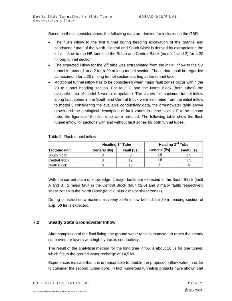
• Additional tunnel inflow has to be considered when major fault zones occur within the 20 m tunnel heading section. For fault C and the North Block (both tubes) the available data of model 3 were extrapolated. The values for maximum tunnel inflow along fault zones in the South and Central Block were estimated from the initial inflow to model 3 considering the available conductivity data, the groundwater table above crown and the geological description of fault zones in these blocks. For the second tube, the figures of the first tube were reduced. The following table show the flush tunnel inflow for sections with and without fault zones for both tunnel tubes.
Table 9: Flush tunnel inflow
Heading 1st Tube Heading 2nd Tube Tectonic unit General [l/s] Fault [l/s] General [l/s] Fault [l/s] South block 3 8 1,5 3.5 Central block 3 12 1,5 3.5 North Block 3 15 1 6
With the current state of knowledge, 2 major faults are expected in the South Block (fault A and B), 1 major fault in the Central Block (fault 02-5) and 3 major faults respectively shear zones in the North Block (fault C plus 2 major shear zones).
During construction a maximum steady state inflow behind the 20m heading section of app. 50 l/s is expected.
7.2 Steady State Groundwater Inflow
After completion of the final lining, the ground water table is expected to reach the steady state even for layers with high hydraulic conductivity.
The result of the analytical method for the long time inflow is about 16 l/s for one tunnel, which fits to the ground water recharge of 14,5 l/s.
Experiences indicate that it is unreasonable to double the proposed inflow value in order to consider the second tunnel bore. In fact numerous tunneling projects have shown that

D e v i l s S l i d e T u n n e l D e v i l ’ s S l i d e T u n n e l I 0 0 5 / A D - 0 4 2 / F I N A L G e o h y d r o l o g i c S t u d y
I L F C O N S U L T I N G E N G I N E E R S P a g e 28 ILF/I P:\Devils Slide\Geohydrology Study\ad_42_FINAL_091505.doc
the groundwater inflow increases by the amount of 20% due to the second bore ([10] and [17]). This would result in a steady state inflow of approximately 20 l/s for both tunnels. In order to consider the fluctuation of the annual precipitation ratio (dry and wet years) a supplement of 50 % is added, resulting in a final figure for steady state inflow of 30 l/s for both tunnel tubes.

D e v i l s S l i d e T u n n e l D e v i l ’ s S l i d e T u n n e l I 0 0 5 / A D - 0 4 2 / F I N A L G e o h y d r o l o g i c S t u d y
I L F C O N S U L T I N G E N G I N E E R S P a g e 29 ILF/I P:\Devils Slide\Geohydrology Study\ad_42_FINAL_091505.doc
8 REFERENCES
1. Bicknelli, B., Imhoff, J., Kitte, J., Donigan, A. & Johanson, R. (1997):Hydrological Simulation Program – Fortran. User’s Manual for Version 11: EPA/600/R-97/080.
2. California Irrigation Management Information System (CIMIS): Map of Reference Evapotranspiration, 1999 (available online from: http://wwwcimis.water.ca.gov/cimis/infoEtoOverview.jsp).
3. California Cooperative Snow Surveys: WY Monthly Precipitation (All Stations) (available online from : http://cdec. water.ca.gov/cgi-progs/printfv/PRECIPOUT.2003.html)
4. Devil’s Slide Tunnel Study: Appendix II of X Volume 1, 2 and 3 of 3, Exploration Data Memorandum, Woodward-Clyde: Sep. 1996
5. Devil’s Slide Tunnel Project: Geologic and Geotechnical Data Report, Volume 3 – In Situ Testing, EMI: Dec. 9, 2002
6. Devil’s Slide Tunnel Project: Phase 2A Geologic Investigation, draft, EMI: October 2001
7. Devil’s Slide Tunnel Project: Phase 2A Supplemental Geologic Investigation, EMI: March 2002
8. Devil’s Slide Tunnel Project: Interpreted Geologic, Geotechnical and Hydrogeological Conditions, final, EMI: May 27, 2004
9. Devil’s Slide Tunnel Project: Figure 1-6: Longitudinal Profile along Centreline between Tunnel Alignments with Interpreted Engineering Parameters along Tunnel Bores, EMI: May 27, 2004
10. Devil’s Slide Tunnel Project: Predicted Groundwater Inflows into the Devil’s Slide Tunnel Using Heuer’s Method. Memorandum by Gregg Korbin, 2004
11. Devil’s Slide Tunnel Project: Geohydraulic Analysis and Ground Water Flow Model of the Proposed Devil’s Slide Tunnel, GEOSCIENCE Support Services, Inc, August 2001.
12. El Tani, M. (1999): Water inflow into tunnels. World Tunnel Congress – Challenges for the 21st Century.
13. EMI (2004): Groundwater Monitoring Data of 11 Piezometers along the tunnel alignment
14. Goodman, R.E. (1965): Ground Water Inflow into a Tunnel Drive. Bulletin of the Association of Engineering Geologists 2(1): 41-56.
15. Herth, W. & Arndts, E. (1973): Theorie und Praxis der Grundwasserabsenkung. Berlin, Ernst & Sohn.
16. Lei, S. (1999): An analytical solution for steady state flow into a tunnel. - Ground Water, Vol. 37 (1): 23-26.
17. Löw, S. (2002): Groundwater hydraulics and environmental impacts of tunnel in crystalline rocks. In: Barla, G. & Barla, M. Bologna (eds.): Le opere in sotterraneo e il rapporto con l'ambiente. 201-218. Patron Editore
D e v i l s S l i d e T u n n e l D e v i l ’ s S l i d e T u n n e l I 0 0 5 / A D - 0 4 2 / F I N A L G e o h y d r o l o g i c S t u d y
I L F C O N S U L T I N G E N G I N E E R S P a g e 30 ILF/I P:\Devils Slide\Geohydrology Study\ad_42_FINAL_091505.doc
18. Prinz, H. (1997): Abriß der Ingenieurgeologie. - 3., neu bearb. und erw. Aufl.. – Stuttgart, Enke.
19. Polubarinova-Kochina, P. Ya (1962): Theory of Ground Water Movement. Princeton, Princeton University. Thiem, G. (1906): Hydrogeologische Methoden. Leipzig, Gebhardt.

D e v i l s S l i d e T u n n e l D e v i l ’ s S l i d e T u n n e l I 0 0 5 / A D - 0 4 2 / F I N A L G e o h y d r o l o g i c S t u d y
I L F C O N S U L T I N G E N G I N E E R S P a g e 31 ILF/I P:\Devils Slide\Geohydrology Study\ad_42_FINAL_091505.doc
Appendix 1: Groundwater Monitoring Data

D e v i l s S l i d e T u n n e l D e v i l ’ s S l i d e T u n n e l I 0 0 5 / A D - 0 4 2 / F I N A L G e o h y d r o l o g i c S t u d y
I L F C O N S U L T I N G E N G I N E E R S P a g e 32 ILF/I P:\Devils Slide\Geohydrology Study\ad_42_FINAL_091505.doc
Groundwater Monitoring Data of the 1996 Piezometers [1]
DATE[ft] [m] [ft] [m] [ft] [m] [ft] [m] [ft] [m] [ft] [m] [ft] [m] [ft] [m]
12.09.2001 216.84 66.11 373.48 113.86 424.90 129.54 199.37 60.78 217.00 66.1624.10.2001 218.93 66.75 372.70 113.63 425.11 129.60 198.69 60.57 216.60 66.0327.11.2001 220.09 67.10 372.19 113.47 425.15 129.62 199.32 60.77 216.82 66.1029.01.2002 223.40 68.11 375.00 114.33 425.65 129.77 203.47 62.03 220.68 67.2826.02.2002 224.95 68.58 375.00 114.33 425.62 129.76 203.77 62.12 222.76 67.9127.03.2002 222.67 67.89 375.00 114.33 426.00 129.87 203.85 62.15 221.36 67.4929.04.2002 221.33 67.48 375.00 114.33 426.20 129.94 202.95 61.87 220.10 67.1030.05.2002 220.56 67.24 375.00 114.33 426.35 129.98 202.32 61.68 219.38 66.8828.06.2002 220.99 67.37 375.00 114.33 426.40 130.00 201.75 61.51 218.85 66.7226.07.2002 218.71 66.68 375.00 114.33 426.40 130.00 201.15 61.32 218.48 66.6130.08.2002 219.24 66.84 375.00 114.33 426.37 129.99 201.00 61.28 218.62 66.6527.09.2002 219.76 67.00 375.00 114.33 426.65 130.07 200.59 61.15 218.33 66.5604.11.2002 219.68 66.97 375.00 114.33 426.48 130.02 200.00 60.97 217.48 66.30 284.14 86.63 250.90 76.49 212.82 64.8826.11.2002 220.51 67.23 375.00 114.33 426.67 130.08 200.35 61.08 217.58 66.3330.12.2002 229.00 69.81 375.00 114.33 426.82 130.12 203.32 61.99 221.62 67.5731.01.2003 223.15 68.03 375.00 114.33 426.80 130.12 203.52 62.05 220.32 67.1728.02.2003 232.38 70.85 375.00 114.33 426.88 130.14 203.89 62.16 222.80 67.9328.03.2003 223.33 68.09 427.25 130.2630.04.2003 223.27 68.07 375.00 114.33 427.12 130.22 203.89 62.16 221.09 67.4030.05.2003 222.19 67.74 375.00 114.33 427.30 130.27 203.55 62.06 220.64 67.2730.06.2003 219.24 66.84 375.00 114.33 427.21 130.24 202.36 61.69 219.46 66.9131.07.2003 220.05 67.09 375.00 114.33 427.35 130.29 201.42 61.41 218.82 66.7129.08.2003 219.30 66.86 427.19 130.24 200.69 61.18 218.32 66.5630.09.2003 219.45 66.90 427.12 130.22 200.15 61.02 217.97 66.4530.10.2003 217.82 66.41 427.18 130.23 199.48 60.82 217.60 66.3426.11.2003 219.62 66.96 427.00 130.18 199.30 60.76 217.36 66.2705.01.2004 237.99 72.56 427.04 130.19 202.90 61.86 222.59 67.8628.01.2004 223.09 68.01 426.98 130.17 203.12 61.93 220.12 67.1127.02.2004 241.83 73.73 426.98 130.17 204.65 62.39 223.57 68.1631.03.2004 223.04 68.00 427.08 130.20 203.70 62.10 220.72 67.2930.04.2004 219.31 66.86 426.86 130.14 202.70 61.80 219.67 66.9730.06.2004 218.02 66.47 427.78 130.42 201.18 61.33 218.50 66.6129.07.2004 219.70 66.98 427.95 130.47 200.67 61.18 218.10 66.4931.08.2004 217.95 66.45 427.83 130.43 200.27 61.06 217.71 66.37Minimum 216.84 66.11 372.19 113.47 424.90 129.54 198.69 60.57 216.60 66.03Maximum 241.83 73.73 375.00 114.33 427.95 130.47 204.65 62.39 223.57 68.16
Mean 222.28 67.77 374.68 114.23 426.70 130.09 201.80 61.52 219.42 66.90Median 220.30 67.16 375.00 114.33 426.87 130.14 201.75 61.51 218.85 66.72
Stand. Deviation 5.47 1.67 0.82 0.25 0.75 0.23 1.72 0.52 1.90 0.58
P-2-96 P-7-96 P-9-96 P-10-96 P-11-96 B-5 B-7 B-9WATER SURFACE ELEVATION - ft (APPROX.)
D e v i l s S l i d e T u n n e l D e v i l ’ s S l i d e T u n n e l I 0 0 5 / A D - 0 4 2 / F I N A L G e o h y d r o l o g i c S t u d y
I L F C O N S U L T I N G E N G I N E E R S P a g e 33 ILF/I P:\Devils Slide\Geohydrology Study\ad_42_FINAL_091505.doc
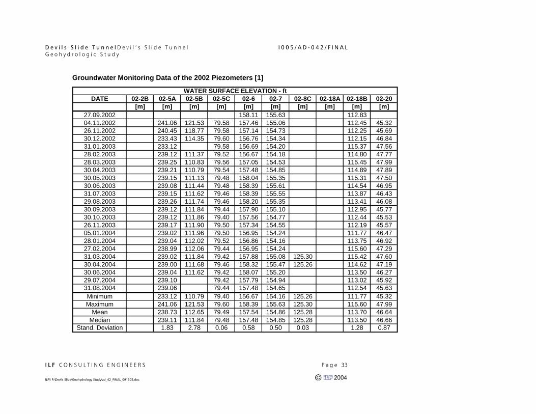
Groundwater Monitoring Data of the 2002 Piezometers [1]
DATE 02-2B 02-5A 02-5B 02-5C 02-6 02-7 02-8C 02-18A 02-18B 02-20[m] [m] [m] [m] [m] [m] [m] [m] [m] [m]
27.09.2002 158.11 155.63 112.8304.11.2002 241.06 121.53 79.58 157.46 155.06 112.45 45.3226.11.2002 240.45 118.77 79.58 157.14 154.73 112.25 45.6930.12.2002 233.43 114.35 79.60 156.76 154.34 112.15 46.8431.01.2003 233.12 79.58 156.69 154.20 115.37 47.5628.02.2003 239.12 111.37 79.52 156.67 154.18 114.80 47.7728.03.2003 239.25 110.83 79.56 157.05 154.53 115.45 47.9930.04.2003 239.21 110.79 79.54 157.48 154.85 114.89 47.8930.05.2003 239.15 111.13 79.48 158.04 155.35 115.31 47.5030.06.2003 239.08 111.44 79.48 158.39 155.61 114.54 46.9531.07.2003 239.15 111.62 79.46 158.39 155.55 113.87 46.4329.08.2003 239.26 111.74 79.46 158.20 155.35 113.41 46.0830.09.2003 239.12 111.84 79.44 157.90 155.10 112.95 45.7730.10.2003 239.12 111.86 79.40 157.56 154.77 112.44 45.5326.11.2003 239.17 111.90 79.50 157.34 154.55 112.19 45.5705.01.2004 239.02 111.96 79.50 156.95 154.24 111.77 46.4728.01.2004 239.04 112.02 79.52 156.86 154.16 113.75 46.9227.02.2004 238.99 112.06 79.44 156.95 154.24 115.60 47.2931.03.2004 239.02 111.84 79.42 157.88 155.08 125.30 115.42 47.6030.04.2004 239.00 111.68 79.46 158.32 155.47 125.26 114.62 47.1930.06.2004 239.04 111.62 79.42 158.07 155.20 113.50 46.2729.07.2004 239.10 79.42 157.79 154.94 113.02 45.9231.08.2004 239.06 79.44 157.48 154.65 112.54 45.63Minimum 233.12 110.79 79.40 156.67 154.16 125.26 111.77 45.32Maximum 241.06 121.53 79.60 158.39 155.63 125.30 115.60 47.99
Mean 238.73 112.65 79.49 157.54 154.86 125.28 113.70 46.64Median 239.11 111.84 79.48 157.48 154.85 125.28 113.50 46.66
Stand. Deviation 1.83 2.78 0.06 0.58 0.50 0.03 1.28 0.87
WATER SURFACE ELEVATION - ft

D e v i l s S l i d e T u n n e l D e v i l ’ s S l i d e T u n n e l I 0 0 5 / A D - 0 4 2 / F I N A L G e o h y d r o l o g i c S t u d y
I L F C O N S U L T I N G E N G I N E E R S P a g e 34 ILF/I P:\Devils Slide\Geohydrology Study\ad_42_FINAL_091505.doc
Hydrographs of Piezometers at the South Portal Area
Groundwater Table South Portal
0
10
20
30
40
50
60
70
8019
.04.
01
05.1
1.01
24.0
5.02
10.1
2.02
28.0
6.03
14.0
1.04
01.0
8.04
17.0
2.05
Date
Elev
atio
n ab
ove
Sea
Leve
l [m
]
02-20P-2-96
Hydrographs of Piezometers at the North Portal Area
Groundwater Table North Portal
0
20
40
60
80
100
120
140
19.0
4.01
05.1
1.01
24.0
5.02
10.1
2.02
28.0
6.03
14.0
1.04
01.0
8.04
17.0
2.05
Date
Elev
atio
n ab
ove
Sea
Leve
l [m
]
02-18BP-7-96P-10-96P-11-96
D e v i l s S l i d e T u n n e l D e v i l ’ s S l i d e T u n n e l I 0 0 5 / A D - 0 4 2 / F I N A L G e o h y d r o l o g i c S t u d y
I L F C O N S U L T I N G E N G I N E E R S P a g e 35 ILF/I P:\Devils Slide\Geohydrology Study\ad_42_FINAL_091505.doc
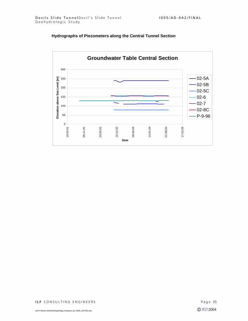
Hydrographs of Piezometers along the Central Tunnel Section
Groundwater Table Central Section
0
50
100
150
200
250
30019
.04.
01
05.1
1.01
24.0
5.02
10.1
2.02
28.0
6.03
14.0
1.04
01.0
8.04
17.0
2.05
Date
Elev
atio
n ab
ove
Sea
Leve
l [m
] 02-5A02-5B02-5C02-602-702-8CP-9-96

D e v i l s S l i d e T u n n e l D e v i l ’ s S l i d e T u n n e l I 0 0 5 / A D - 0 4 2 / F I N A L G e o h y d r o l o g i c S t u d y
I L F C O N S U L T I N G E N G I N E E R S P a g e 36 ILF/I P:\Devils Slide\Geohydrology Study\ad_42_FINAL_091505.doc
Appendix 2: Results of the Analytical Tunnel Inflow Calculations
D e v i l s S l i d e T u n n e l D e v i l ’ s S l i d e T u n n e l I 0 0 5 / A D - 0 4 2 / F I N A L G e o h y d r o l o g i c S t u d y
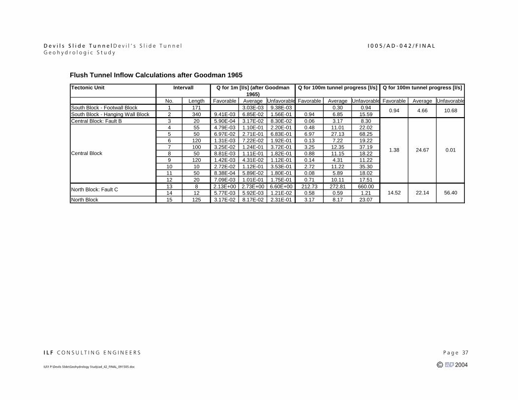
I L F C O N S U L T I N G E N G I N E E R S P a g e 37 ILF/I P:\Devils Slide\Geohydrology Study\ad_42_FINAL_091505.doc
Flush Tunnel Inflow Calculations after Goodman 1965
Tectonic Unit
No. Length Favorable Average Unfavorable Favorable Average Unfavorable Favorable Average UnfavorableSouth Block - Footwall Block 1 171 3.03E-03 9.38E-03 0.30 0.94South Block - Hanging Wall Block 2 340 9.41E-03 6.85E-02 1.56E-01 0.94 6.85 15.59Central Block: Fault B 3 20 5.90E-04 3.17E-02 8.30E-02 0.06 3.17 8.30
4 55 4.79E-03 1.10E-01 2.20E-01 0.48 11.01 22.025 50 6.97E-02 2.71E-01 6.83E-01 6.97 27.13 68.256 120 1.31E-03 7.22E-02 1.92E-01 0.13 7.22 19.227 100 3.25E-02 1.24E-01 3.72E-01 3.25 12.35 37.198 50 8.81E-03 1.11E-01 1.82E-01 0.88 11.15 18.229 120 1.42E-03 4.31E-02 1.12E-01 0.14 4.31 11.2210 10 2.72E-02 1.12E-01 3.53E-01 2.72 11.22 35.3011 50 8.38E-04 5.89E-02 1.80E-01 0.08 5.89 18.0212 20 7.09E-03 1.01E-01 1.75E-01 0.71 10.11 17.5113 8 2.13E+00 2.73E+00 6.60E+00 212.73 272.81 660.0014 12 5.77E-03 5.92E-03 1.21E-02 0.58 0.59 1.21
North Block 15 125 3.17E-02 8.17E-02 2.31E-01 3.17 8.17 23.0714.52 22.14 56.40
4.66 10.68
1.38 24.67 0.01Central Block
North Block: Fault C
Q for 1m [l/s] (after Goodman 1965)
Intervall Q for 100m tunnel progress [l/s]
0.94
Q for 100m tunnel progress [l/s]

D e v i l s S l i d e T u n n e l D e v i l ’ s S l i d e T u n n e l I 0 0 5 / A D - 0 4 2 / F I N A L G e o h y d r o l o g i c S t u d y
I L F C O N S U L T I N G E N G I N E E R S P a g e 38 ILF/I P:\Devils Slide\Geohydrology Study\ad_42_FINAL_091505.doc
Flush Tunnel Inflow Calculations after Jacob & Lohmann 1952 Tectonic Unit Storativity
No. Length Favorable Average Unfavorable Favorable Average Unfavorable Favorable Average UnfavorableSouth Block - Footwall Block 1 171 0.01 3.61E-03 0.36South Block - Hanging Wall Block 2 340 0.01 6.57E-03 7.28E-02 2.06E-01 0.66 7.28 20.57Central Block: Fault B 3 25 0.05 2.20E-04 1.98E-02 6.29E-02 0.02 1.98 6.29
4 50 0.05 2.06E-03 9.09E-02 2.64E-01 0.21 9.09 26.355 50 0.1 6.13E-02 8.81E-02 8.51E-01 6.13 8.81 85.136 120 0.05 7.84E-04 6.35E-02 2.18E-01 0.08 6.35 21.847 100 0.1 2.37E-02 1.14E-01 4.19E-01 2.37 11.40 41.928 50 0.05 5.77E-03 9.25E-02 2.04E-01 0.58 9.25 20.399 120 0.1 7.05E-04 3.39E-02 1.06E-01 0.07 3.39 10.5910 10 0.1 1.82E-02 5.34E-02 3.90E-01 1.82 5.34 39.0311 50 0.05 4.01E-04 5.16E-02 1.98E-01 0.04 5.16 19.8012 20 0.05 4.12E-03 4.38E-02 7.22E-02 0.41 4.38 7.2213 8 0.2 1.80E+00 1.80E+00 4.27E+00 180.37 180.37 427.0014 12 0.05 2.27E-03 2.27E-03 4.91E-03 0.23 0.23 0.49
North Block 15 125 0.05 3.08E-03 3.44E-02 1.17E-01 0.31 3.44 11.67
1.06 6.92 27.49
10.24 12.93 33.66
Q for 100m tunnel progress [l/s]
0.44 4.85 13.81
Intervall
Central Block
North Block: Fault C
Q for 1m [l/s] (after Jacob & Lohmann 1952)
Q for 100m tunnel progress [l/s]

D e v i l s S l i d e T u n n e l D e v i l ’ s S l i d e T u n n e l I 0 0 5 / A D - 0 4 2 / F I N A L G e o h y d r o l o g i c S t u d y
I L F C O N S U L T I N G E N G I N E E R S P a g e 39 ILF/I P:\Devils Slide\Geohydrology Study\ad_42_FINAL_091505.doc
Steady State Tunnel Inflow Calculations using Cylinder Formula
Tectonic Unit
No. Length Favorable Average Unfavorable Favorable Average UnfavorableSouth Block - Footwall Block 1 171 8.09E-05 1.97E-03 6.69E-03 0.01 0.34 1.14South Block - Hanging Wall Block 2 340 3.87E-03 2.23E-02 4.22E-02 1.32 7.57 14.36Central Block: Fault B 3 25 3.03E-04 1.44E-02 3.41E-02 0.01 0.36 0.85
4 50 2.64E-03 2.52E-02 3.34E-02 0.13 1.26 1.675 50 1.38E-02 5.04E-02 1.20E-01 0.69 2.52 5.986 120 3.03E-04 1.44E-02 3.41E-02 0.04 1.73 4.107 100 8.80E-03 2.66E-02 6.69E-02 0.88 2.66 6.698 50 2.64E-03 2.52E-02 3.34E-02 0.13 1.26 1.679 120 4.57E-04 1.02E-02 2.11E-02 0.05 1.22 2.5310 10 8.80E-03 2.66E-02 6.69E-02 0.09 0.27 0.6711 50 3.03E-04 1.44E-02 3.41E-02 0.02 0.72 1.7112 20 2.64E-03 2.52E-02 3.34E-02 0.05 0.50 0.6713 814 12
North Block 15 125Sum
Q for tunnel section [l/s]Intervall
Central Block
North Block: Fault C
Q for 1m [l/s] (Cylindric tunnel)
NOT APPLICABLE NOT APPLICABLE
Cumulative Steady State Tunnel Inflow using Cylinder Formula
Cumulativ Steady State Tunnel Inflow (Cylinder Formula)
Nor
th P
orta
l
Faul
t C
Faul
t B
Sout
h Po
rtal
01020304050607080
1180
0
1200
0
1220
0
1240
0
1260
0
1280
0
1300
0
1320
0
Station [m]
Q [l
/s] Favorable
Average
Unfavorable
D e v i l s S l i d e T u n n e l D e v i l ’ s S l i d e T u n n e l I 0 0 5 / A D - 0 4 2 / F I N A L G e o h y d r o l o g i c S t u d y
I L F C O N S U L T I N G E N G I N E E R S P a g e 40 ILF/I P:\Devils Slide\Geohydrology Study\ad_42_FINAL_091505.doc
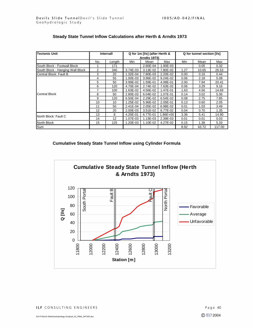
Steady State Tunnel Inflow Calculations after Herth & Arndts 1973
Tectonic Unit
No. Length Min Mean Max Min Mean MaxSouth Block - Footwall Block 1 171 2.80E-04 1.90E-03 0.05 0.32South Block - Hanging Wall Block 2 340 3.74E-03 3.13E-02 7.80E-02 1.27 10.65 26.53Central Block: Fault B 3 20 1.32E-04 7.80E-03 2.20E-02 0.00 0.16 0.44
4 55 1.00E-03 3.96E-02 9.24E-02 0.06 2.18 5.085 50 3.99E-02 1.59E-01 4.08E-01 2.00 7.94 20.416 120 4.70E-04 2.74E-02 7.63E-02 0.06 3.29 9.167 100 1.63E-02 4.56E-02 1.47E-01 1.63 4.56 14.698 50 2.80E-03 6.04E-02 1.07E-01 0.14 3.02 5.369 120 6.50E-04 2.29E-02 6.54E-02 0.08 2.75 7.8510 10 1.25E-02 5.96E-02 2.05E-01 0.13 0.60 2.0511 50 2.41E-04 2.05E-02 6.98E-02 0.01 1.03 3.4912 20 2.00E-03 3.51E-02 6.77E-02 0.04 0.70 1.3513 8 4.20E-01 6.77E-01 1.86E+00 3.36 5.41 14.9014 12 1.07E-03 1.13E-03 2.39E-03 0.01 0.01 0.03
North Block 15 125 1.20E-03 1.10E-02 4.27E-02 0.15 1.38 5.33Sum 8.92 43.72 117.00
North Block: Fault C
Q for tunnel section [l/s]Q for 1m [l/s] (after Herth & Arndts 1973)
Intervall
Central Block
Cumulative Steady State Tunnel Inflow using Cylinder Formula
Cumulative Steady State Tunnel Inflow (Herth & Arndts 1973)N
orth
Por
tal
Faul
t C
Faul
t B
Sout
h Po
rtal
0
20
40
60
80
100
120
1180
0
1200
0
1220
0
1240
0
1260
0
1280
0
1300
0
1320
0
Station [m]
Q [l
/s] Favorable
Average
Unfavorable

D e v i l s S l i d e T u n n e l D e v i l ’ s S l i d e T u n n e l I 0 0 5 / A D - 0 4 2 / F I N A L G e o h y d r o l o g i c S t u d y
I L F C O N S U L T I N G E N G I N E E R S P a g e 41 ILF/I P:\Devils Slide\Geohydrology Study\ad_42_FINAL_091505.doc
Appendix 3: Results of the Numerical Tunnel Inflow Calculations
D e v i l s S l i d e T u n n e l D e v i l ’ s S l i d e T u n n e l I 0 0 5 / A D - 0 4 2 / F I N A L G e o h y d r o l o g i c S t u d y
I L F C O N S U L T I N G E N G I N E E R S P a g e 42 ILF/I P:\Devils Slide\Geohydrology Study\ad_42_FINAL_091505.doc
D e v i l s S l i d e T u n n e l D e v i l ’ s S l i d e T u n n e l I 0 0 5 / A D - 0 4 2 / F I N A L G e o h y d r o l o g i c S t u d y
I L F C O N S U L T I N G E N G I N E E R S P a g e 43 ILF/I P:\Devils Slide\Geohydrology Study\ad_42_FINAL_091505.doc

D e v i l s S l i d e T u n n e l D e v i l ’ s S l i d e T u n n e l I 0 0 5 / A D - 0 4 2 / F I N A L G e o h y d r o l o g i c S t u d y
I L F C O N S U L T I N G E N G I N E E R S P a g e 44 ILF/I P:\Devils Slide\Geohydrology Study\ad_42_FINAL_091505.doc

D e v i l s S l i d e T u n n e l D e v i l ’ s S l i d e T u n n e l I 0 0 5 / A D - 0 4 2 / F I N A L G e o h y d r o l o g i c S t u d y
I L F C O N S U L T I N G E N G I N E E R S P a g e 45 ILF/I P:\Devils Slide\Geohydrology Study\ad_42_FINAL_091505.doc
D e v i l s S l i d e T u n n e l D e v i l ’ s S l i d e T u n n e l I 0 0 5 / A D - 0 4 2 / F I N A L G e o h y d r o l o g i c S t u d y
I L F C O N S U L T I N G E N G I N E E R S P a g e 46 ILF/I P:\Devils Slide\Geohydrology Study\ad_42_FINAL_091505.doc

D e v i l s S l i d e T u n n e l D e v i l ’ s S l i d e T u n n e l I 0 0 5 / A D - 0 4 2 / F I N A L G e o h y d r o l o g i c S t u d y
I L F C O N S U L T I N G E N G I N E E R S P a g e 47 ILF/I P:\Devils Slide\Geohydrology Study\ad_42_FINAL_091505.doc

D e v i l s S l i d e T u n n e l D e v i l ’ s S l i d e T u n n e l I 0 0 5 / A D - 0 4 2 / F I N A L G e o h y d r o l o g i c S t u d y
I L F C O N S U L T I N G E N G I N E E R S P a g e 48 ILF/I P:\Devils Slide\Geohydrology Study\ad_42_FINAL_091505.doc
D e v i l s S l i d e T u n n e l D e v i l ’ s S l i d e T u n n e l I 0 0 5 / A D - 0 4 2 / F I N A L G e o h y d r o l o g i c S t u d y
I L F C O N S U L T I N G E N G I N E E R S P a g e 49 ILF/I P:\Devils Slide\Geohydrology Study\ad_42_FINAL_091505.doc

D e v i l s S l i d e T u n n e l D e v i l ’ s S l i d e T u n n e l I 0 0 5 / A D - 0 4 2 / F I N A L G e o h y d r o l o g i c S t u d y
I L F C O N S U L T I N G E N G I N E E R S P a g e 50 ILF/I P:\Devils Slide\Geohydrology Study\ad_42_FINAL_091505.doc

D e v i l s S l i d e T u n n e l D e v i l ’ s S l i d e T u n n e l I 0 0 5 / A D - 0 4 2 / F I N A L G e o h y d r o l o g i c S t u d y
I L F C O N S U L T I N G E N G I N E E R S P a g e 51 ILF/I P:\Devils Slide\Geohydrology Study\ad_42_FINAL_091505.doc
Appendix 4: Tunnel Inflow Calculations by Greg Korbin using Heuer’s Method