AD-A212 692

AFGL-TR-88-0032ENVIRONMENTAL RESEARCH PAPERS, NO. 994

* Short Term Forecasting of Cloud and Precipitation

A. BOHNEF.I. HARRISP.A. SADOSKID. EGERTON

.15 January 1988

Approved for public release; distribution unlimited.

DTIC*g LICT E

S_ E I 1 i389

ATMOSPHERIC SCIENCES DIVISION PROJECT 6670

AIR FORCE GEOPHYSICS LABORATORYHANSCOM AFB, MA 01731

89 9 20 016

"This technical report has been reviewed and is approved forpublication"

FOR THE COMMANDER

KENPETH M. GLOVER, Chief RMERT A. .CCLATCHEY, Direc rGround Based Remote Sensing Branch Atmospheric Sciences DivisionAtmospheric Sciences Division

This document has been reviewed by the ESD Public Affairs Office (PA)and is releasable to the National Technical Information Service(NTIS).

Qualified requestors may obtain additional copies from the DefenseTechnical Information Center. All others should epply to theNational Technical Information Service.

If your address has changed, or if you wish to be removed from themailing list, or if the addressee is no longer employed by yourorganization, please notify AFGL/DAA, Hanscom AFB, MA 01731. Thiswill assist us in maintaining a current mailing list.

UNCLASSIFIEDSECURITY CLASSFICATION OF THIS PAGE

REPORT DOCUMENTATION PAGE Form ApprovedOMB No. 0704-0188

Ia. REPORT SECURITY CLASSIFICATION lb. RESTRICTIVE MARKINGSUnclassified

2& SECURITY CLASSIFICATION AUTHORITY 3. DISTRIBUTION i AVAILABILITY OF REPORT

Approved for public release;2b. DECLASSIFICATION / DOWNGRADING SCHEDULE distribution unlimited.

4. PERFORMING ORGANIZATION REPORT NUMBER(S) S. MONITORING ORGANIZATION REPORT NUMBER(S)

AFGL-TR-88-0032ERP, NO. 994

6a. NAME OF PERFORMING ORGANIZATION 6b. OFFICE SYMBOL 7a. NAME OF MONITORING ORGANIZATIONAir Force Geophysics ( fYRa e)Laboratory LYR

6c. ADDRESS (Cy, Sote, ad ZIP Code) 7b. ADDRESS (City, State and ZIP Code)

Hanscom AFBMassachusetts 01731-5000

Sa. NAME OF FUNDING / SPONSORING 8b. OFFICE SYMBOL 9. PROCUREMENT INSTRUMENT IDENTIFICATION NUMBERORGANIZATION (If applicable)

Sc. ADDRESS (Ci State, ad ZIP Code) 10. SOURCE OF FUNDING NUMBERS

PROGRAM PROJECT TASK WORK UNITELEMENT NO. NO. NO. ACCESSION NO.

62101F 6670 10 2111. TITLE (indude Secwiy Classificadn)

Short Term Forecasting of Cloud and Precipitation

12. PERSONAL AUTHOR(S)Bohne, A., Harris F.I.*, Sadoski,P.A., Egerton, D.*

13a. TYPE OF REPORT 13b. TIME COVERED 14. DATE OF REPORT (Yea, Month, Day) 15. PAGE COUNTFinal FROM Sep 86 T0 Sep87 1988 January 15 104

16. SUPPLEMENTARY NOTATION

*ST Systems Corporation, Lexington, Massachusetts

17. COSATI CODES 18. SUBJECT TERMS (Contie on revee If necessary and identity by blodk nub.)

FIELD GROUP SUB-GROUP Nowcastingi Forecasting/ Contour Segmentation,Pattern Recognition , Radar, (..

Extrapolation Data Filtering,19. 1 RACT (Continue on rev*e if necessary and Idendfy by block n~mbe

A methodology for real-time operations has been developed for the short-termforecasting of cloud and precipitation fields. Pattern recognition techniques are employedto extract useful features from the data field and extrapolation techniques are used toproject these features into the future. To reduce computational load, contours defined bydirectional codes are used to delineate features. These contours are subdivided andattributes such as length, location, and location of each segment are determined. Segmentmatching is performed for successive observations and attribute changes are monitored overtime. Several techniques for the forecasting of attributes have been explored, and anexponential smoothing filter and a linear trend adaptive smoothing filter have been chosenas most appropriate. Currently analysis is performed on a minicomputer and image processorsystem utilizing radar reflectivity data. Refinement of these techniques and extensioninto a more comprehensive short term forecasting program is planned. ,

20. DISTRIBUTIONtAVAILABILITY OF ABSTRACT 21. ABSTRACT SECURITY CLASSIFICATIONPIUNCLASSIFIEDUNLIMITED 0 SAME AS RPT. 0 DTIC USERS Unclassified

22a. NAME OF RESPONSIBLE INDIVIDUAL 22b. TELEPHONE (Indude Area Code) 22c. OFFICE SYMBOLAlan R. Bohne 617-377-2943 LYP

DD FORM 1473, JUN 86 Previous edtions are obsolete. SECURITY CLASSIFICATION OF THIS PAGEUNCLASSIFIED

Accession For

NTIS GRA&IDT1C TAS

IUnn:,o. L2ed [

JustifICt io-

SBy-

Av: t . Ccdes

, 'J,11 i I ;j/or

Dt Spcia

v Contents

1. INTRODUCTION 1

2. DATA PREPROCESSING 2

2.1 Data Preprocessing Considerations 22.2 Data Coordinate Transformations 2

2.2.1 Radar Data 32.2.2 Satellite Data 3

2.3 Evolution and Vertical Advection Considerations 42.4 Data Editing 6

2.4.1 Median Filtering 62.4.2 Lowpass Filtering 112.4.3 Feature Editing 112.4.4 Gap Filling 14

3. FEATURE MAPPING AND ATTRIBUTE DEFINITION 14

3.1 Data Source and Feature Forecasting Considerations 143.2 Data Representation Considerations 153.3 Contour Extraction 15

3.3.1 Interpolated Cartesian Contours and Geometric Approximatioti 163.3.2 Freeman Chain Code 17

4. FEATURE MOTION AND EVOLUTION 20

4.1 Introduction to Feature Change Detection 204.2 Orthogonal Vector Method 204.3 Contour Segment Matching 20

4.3.1 Matching Straight Line Segments 224.3.2 Crve Fitting Chain Code Segments 24

4.4 Attribute Determination and Evnlution Detection 27

iii

Contents

5. FORECASTING 27

5.1 Forecasting Considerations 275.2 Candidate Techniques 28

5.2.1 Technique Formulations 285.2.2 Technique Initialization and User Options 32

5.3 Forecast Technique Evaluation with Test Data 345.3.1 Generated Test Data 345.3.2 Real Test Data 47

5.4 Computational Complexity 715.5 Reconstruction 87

6. CONCLUSIONS 87

7. REFERENCES 91

APPENDIX A - FORECASTING ALGORITHMS 93

iv

Illustrations

1. The 32 dBZ reflectivity contour at 5.0 km height at(a) 1052 EST, (b) 1058 EST, (c) 1114 EST, and (d) 1121 EST 5

2. The 32 dBZ reflectivity contour for composited reflectivity - times as in Figure 1 7

3. Windows commonly used with median filters: (a) standard areal filter, (b) gapfilter, and (c) horizontal line filter 8

4. Example of effect of a 3x3 median filter on a binary image 9

5. Same data as in Figure 2 but with a 3x3 median filter applied before contouring 10

6. Commonly used lowpass filters in upper row and RAPID formulation in lower row 12

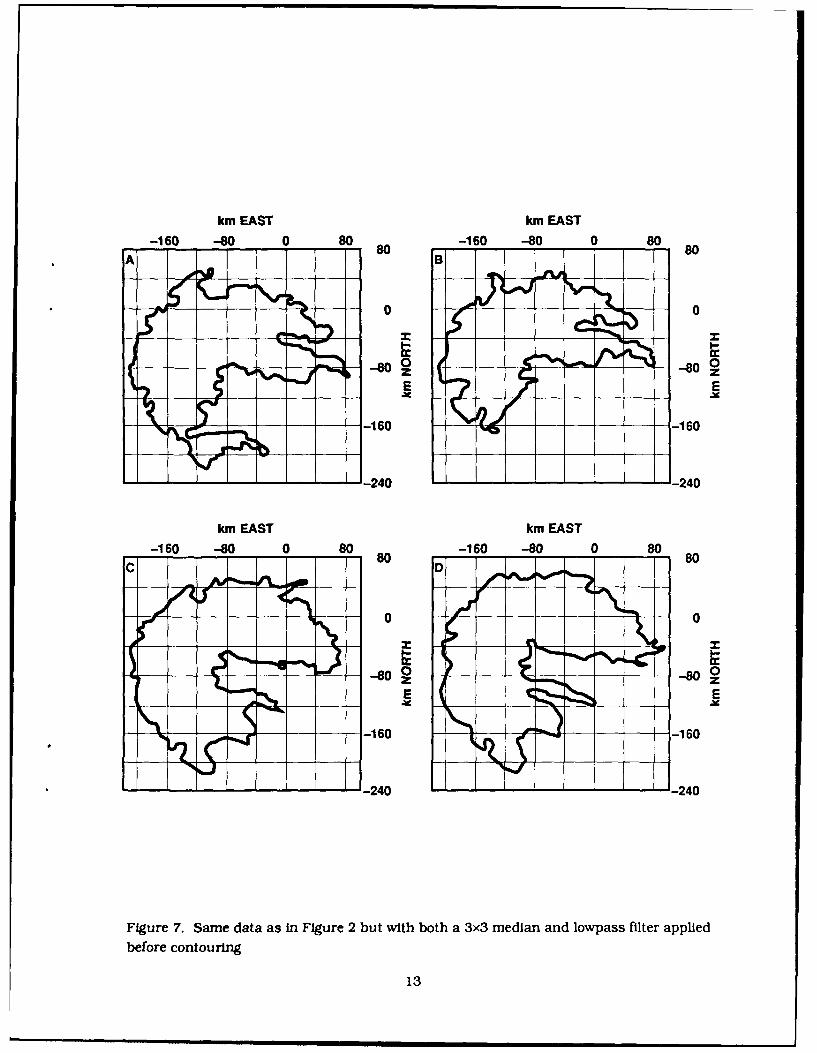
7. Same as in Figure 2 but with both a 3x3 median and lowpass filter applied beforecontouring 13

8. The eight direction vector codes used in the Freeman chain code representation 18

9. A rectangular region of data with a contour boundary defined by the chain code* (3,3,3,5.5,5,5,5,5, 7, 7, 7, 1, 1,, 1, , 1). with origin (1, 1) and length 18 19

10. An example of the Orthogonal Vector Technique. Contours are of infraredtemperature for two scans 30 min apart. The solid contour is for the earlier data.The orthogonal vectors are shown as short dashes 21

11. Evolving rectangular contour of Figure 9 observed at a later time 25

12. Plot of mean difference (solid) and mean square difference (dashed) measurementsresulting from curve fitting a contour segment between two successive times 26

13. Generated test case data for evaluating forecasting routines: (a) stationary data withzero (solid) and negative (dashed) starting values, (b) pure linear, and (c) pure quadraticcases 35

v

Illustrations

14. Plots of actual forecast error for SIMEXP (dash), ADSIMEXP (dash-dot), SIMMOVAV(long/short dash), KALMAN (solid) routines using stationary data (zero start) for(a) one. (b) two, and (c) three-interval forecasts 38

15. Plots of accumulated forecast error corresponding to Figure 14 data 41

16. Plot of forecast error for LINREG method using stationary data (zero start) for one(dash). two (dash-dot), and three-interval (solid) forecasts 46

17. P-oE of foi-ecast error for 13WNQUAD routine using linear data for one (dash), two(dash-dot), and three-interval (solid) forecasts 48

18. Plot of forecast error for BWNQUAD routine using quadratic data for one (dash), two(dash-dot), and three-interval (solid) forecasts 49

19. Plots of center area (COA) image pixel locatiuns for (a) X (east). and (b) Y (north)directions for inner high cirrus area from IR satellite imagery of Hurricane Gloria 52

20. Plot showing the two IR cold dome contours tracked using GOES satellite imagery ofHurricane Gloria: inner (I), and outer (0) contours 54

21. Plots of actual forecast error for SIMEXP (dash), ADSIMEXP (dash-dot), SIMMOVAV(long/short dash), KALMAN (solid) routines using differences of X location data ofFigure 19 for (a) one, (b) two, and (c) three-interval forecasts 55

22. Plots of actual forecast error for SIMEXP (dash), ADSIMEXP (dash-dot), SIMMOVAV(long/short dash). KALMAN (solid) routines using differences of Y location data ofFigure 19 for (a) one, (b) two, and (c) thrce-interval forecasts 58

23. Plots of actual forecast error for LINMOVAV (dash), HOLT2P (dash-dot), BWN 1 PAD(long/short dash), BWNQUAD (solid) routines using X location data of Figure 19 for(a) one, (b) two, and (c) three-interval forecasts 63

24. Plots of actual forecast error for LINMOVAV (dash), HOLT2P (dash-dot), BWN1PAD(long/short dash), BWNQUAD (solid) routines using Y location data of Figure 19 for(a) one, (b) two. and (c) three-interval forecasts 66

25. Plot of forecast error for LINREG method using the position data of Figure 19 for one(dash), two (dash-dot), and three-interval (solid) forecasts: (a) X, and (b) Y position data 69

26. Plots of center of area (COA) image pixel locations for (a) X (east), and (b) Y (north)directions for 32 dBZ contour area from radar observation of Hurricane Gloria 72

27. Plots of actual forecast error for SIMEXP (dash), ADSIMEXP (dash-dot), SIMMOVAV(long/short dash), KALMAN (solid) routines using differences of X location data ofFigure 26 for (a) one. (b) two, and (c) three-interval forecasts 74

28. Plots of actual forecast error for SIMEXP (dash), ADSIMEXP (dash-dot), SIMMOVAV(long/short dash), KALMAN (solid) routines using differences of Y location data ofFigure 26 for (a) one. (b) two. and (c) three-interval forecasts 77

29. Plots of actual forecast error for LINMOVAV (dash), HOLT2P (dash-dot), BWN 1PAD(long/short dash). BWNQUAD (solid) routines using X location data of Figure 26 for(a) one. (b) two, and (c) three-interval forecasts 80

vi

Illustrations

30. Plots of actual forecast error for LINMOVAV (dash), HOLT2P (dash-dot). BWN1PAD(long/short dash), BWNQUAD (solid) routines using Y location data of Figure 26 for(a) one, () two, and (c) three-interval forecasts 83

vii

Tables

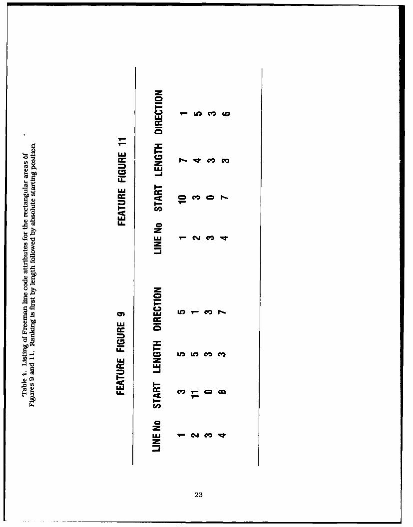
1. Listing of Freeman line code attributes for the rectangular areas of Figures 9 and 11.Ranking is first by length followed by absolute starting position 23

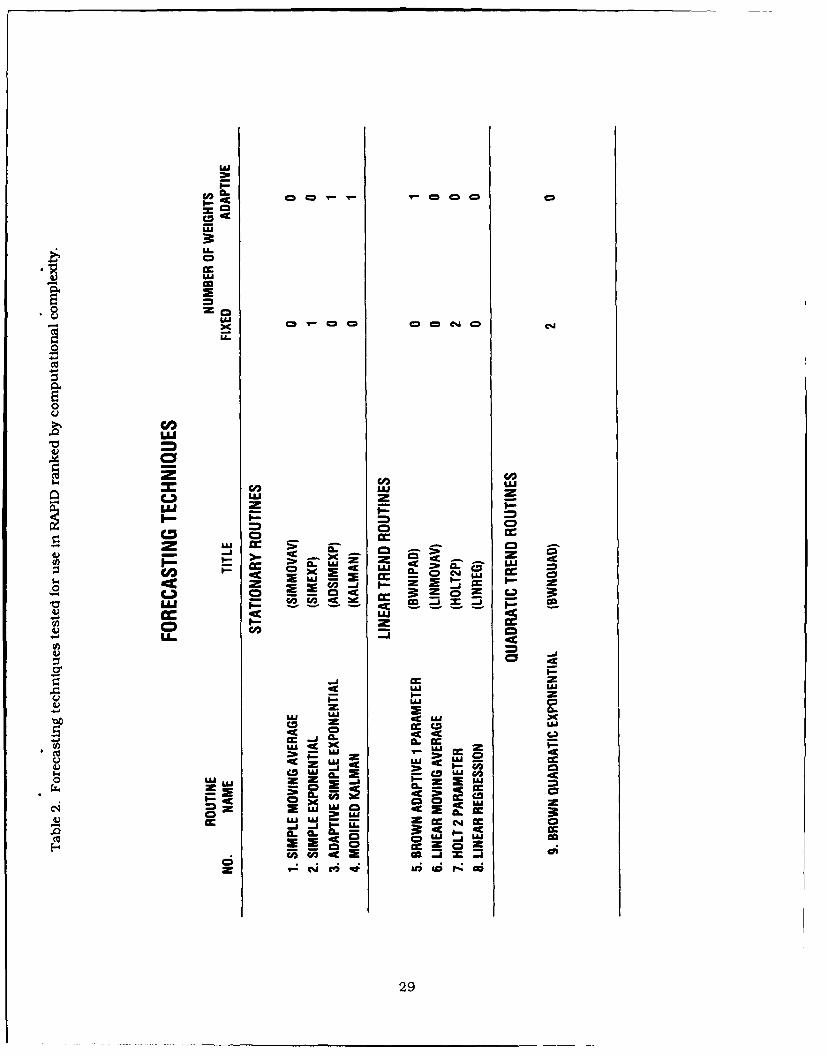
2. Forecasting techniques tested for use in RAPID ranked by computationalcomplexity 29

3. Generic formulations of the ;orecssting techniques listed in Table 2 ranked bycomputational complexity 30

4. Procedures for initializing forecasting techniques listed in Table 2. Techniquemay not develop (none), or may use first observation (obs(1)) as, a first forecastafter first observation. Exact formulation engagement noted by ALGORITHM 33

5. Accumulated absolute forecast error obtained from application of generated testdata with the forecasting techniques. Results for techniques allowing user-selectionof weights are shown for the three weight values W = 0.3, 0.5, and 0.7. 45

6. Accumulated absolute forecast error obtained from application of generated testdifference data with the forecasting techniques. Results for techniques allowing user-selection of weights are shown for the three weight values W = 0.3, 0.5, and 0.7 50

7. Accumulated absolute forecast error obtained from application of Center of Areadata from inner IR contour of Figure 20 with the forecasting techniques. Stationary(nonstationary) techniques employ difference (original) data. Results for techniquesallowing user-selection of weights are shown for the three weight values W = 0.3. 0.5.and 0.7 61

8. Accumulated absolute forecast error obtained from application of Center of Area datafrom outer IR contour of Figure 20 with the forecasting techniques. Stationary(nonstationary) techniques employ difference (original) data. Results for techniquesallowing user-selection of weights are shown for the three weight values W = 0.3, 0.5,and 0.7 62

viii

Tables

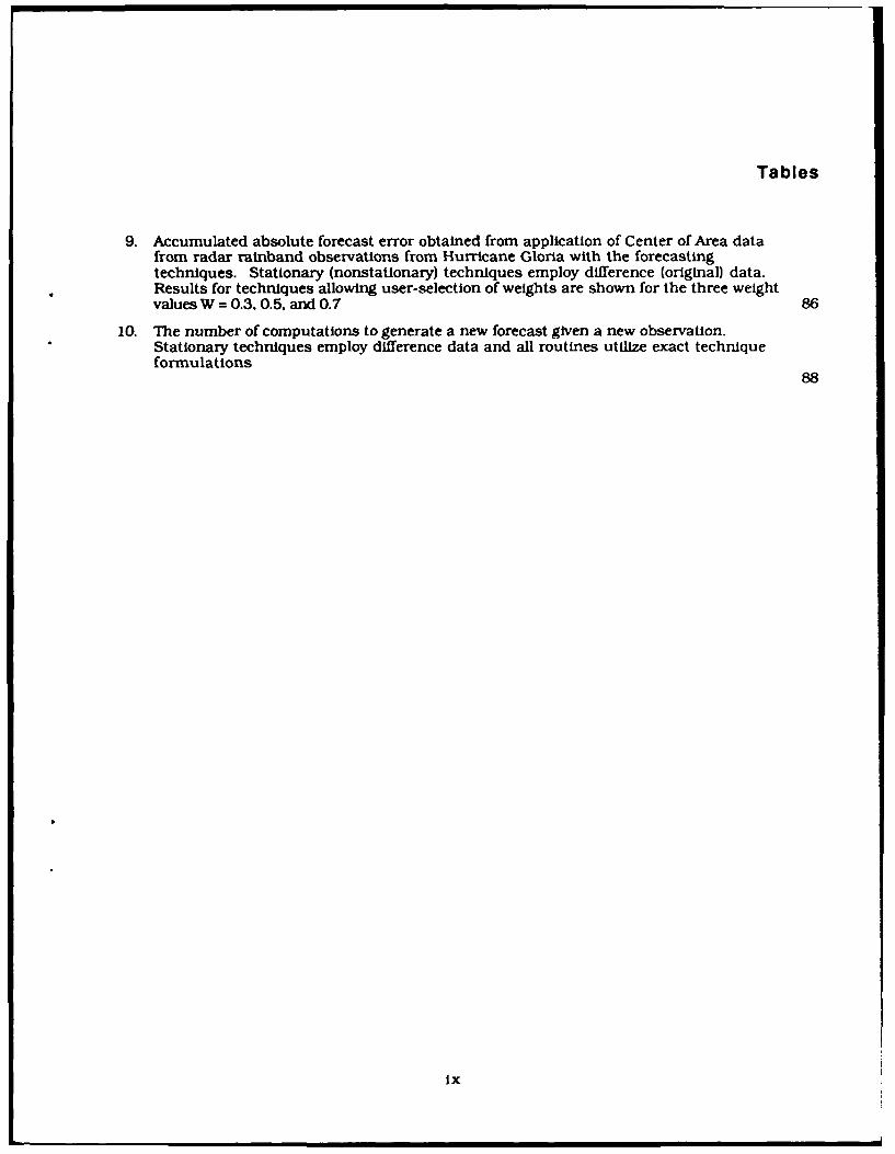
9. Accumulated absolute forecast error obtained from application of Center of Area datafrom radar rainband observations from Hurricane Gloria with the forecastingtechniques. Stationary (nonstationary) techniques employ difference (original) data.Results for techniques allowing user-selection of weights are shown for the three weightvalues W = 0.3, 0.5, and 0.7 86

10. The number of computations to generate a new forecast given a new observation.Stationary techniques employ difference data and all routines utilize exact techniqueformulations

88

ix

Short Term Forecasting ofCloud and Precipitation

1. INTRODUCTION

The Air Force Geophysics Laboratory is developing techniques for accurate nowcasting of cloudand precipitation. Such a capability would be useful in supporting general air and terminaloperations and in predicting periods of communication signal loss. The communication aspect is

particularly important for satellite to ground links utilizing very high frequencies since significantdegradation of signal can result due to intervening cloud or precipitation. The current effortrepresents the development of a computer-based methodology for using continuously updated radar

and satellite data as input for 0 - 0.5 hour forecasts of future cloud and precipitation fields. Theunderlying premise of the procedure Is that future fields may be derived from forecasting selected fieldintensity contours. This requires monitoring the evolving patterns of field intensity and, with

knowledge of the spatial changes of these contours over time, extrapolating to future cloud andprecipitation fields.

The program developed along two lines. One primary effort was the acquisition and integrationof hardware for data assimilation and analysis and the development of a suitable system softwareenvironment. The second effort was the development of the analysis techniques and associatedsoftware. The discussion of hardware and associated system software is presented in a separatereport. I (Sadoski et al. 1987). This report describes the data analysis procedures that have been

developed. A discussion of potential techniques for data analysis and forecasting was presented

(Received for Publication 13 January 1988)

1. Sadoski, P.A., Egerton, D., Harris, F.I, and Bohne, A.R. (1988) The Remote Atmospheric ProbingInformation Display (RAPID), AFGL-TR-88-0036. AD A196314.

1

earlier by Bohne and Harris 2 , where a candidate processing methodology was presented. Themethodology was essentially broken I to four steps: (1) data preprocessing. (2) feature definition andextraction, (3) attribute definition and mapping, and (4), attribute forecasting and featurereconstruction. In this report a discussion of each of these steps will be presented.

2. DATA PREPROCESSING

2.1 Data Preprocessing Considerations

Prior to the application of feature extraction, mapping, and forecasting routines, muchconsideration must be given to providing a data set that supports these efforts. During developmentand testing of potential software techniques, it was quickly realized that successful performance ofthe various methods was correlated with the quality of the input data. Various steps must be employedto develop a well-behaved, yet represe-tative, data set on a suitable coordinate system: specifically,filtering procedures to interpolate data, smooth boundaries, remove errors, and fill gaps must beemployed.

Selection of routines and their specific manner of app~lcation are somewhat dependent upon thehardware environment. The hardware environment is defined by the Remote Atmospheric Processingand Interactive Display (RAPID) System. The RAPID System has as its main components DigitalEquipment Corporation VAX minicomputers, an ADAGE 3000 image processor, and associatedperipherals and communication links. For details regarding the system hardware and software andthe resulting e.ivironment see Sadoski et al. 1 RAPID ingests radar and satellite data from othercomputer systems. These data are then processed and displayed for the forecast problem withinRAPID.

2.2 Data Coordinate Transformations

The raw data received from satellites and radars are in very different coordinate systems. Theradar collects its data in a three-dimensional spherical framework, along radials emanating from theradar itself. The data from the GOES satellite are organized n a distorted planar framework, the

distortion being due to the oblique viewing angle of the satellite sensors relative to the curving earth'ssurface and the mapping of features onto the satellite's flat viewing plane. It is essential that the datafrom these two systems be converted to a common grid if they are to be used together in a quantitativeforecast system. The grid center was chosen to be collocated with the radar at the Ground BasedRemote Sensing Branch (LYR) of AFGL. Because the forecast area is limited to a range of about 250 krmabout the grid center and a regular grid system is most appropriate for data manipulation and displayby the image processor, the grid was selected to be rectangular Cartesian.

2. Bohne, A.R. and Harris, F. Ian (1985) Short Term Forecasting of Cloud and Precipitation,AFGL-TR-85-0343, AD A169744.

2

2.2.1 RADAR DATA

Interpolation of radar data between coordinate systems can be a very computer intensiveoperation in terms of time and memory usage. However, Mohr and Vaughan 3 devised a very efficientalgorithm that minimizes these requirements. Basically, their interpolation algorithm can bedivided into three task areas: data preprocessing, ingestion, and interpolation. In the preprocessingphase the user defines the rectangular Cartesian coordinate system onto which interpolated valueswill be placed. For each Cartesian grid point, the spherical coordinates (range. azimuth, andelevation) are computed. These are then sorted and subsequently stored on disk in the form of levelfiles. Each level file contains the spherical and Cartesian coordinates for all Cartesian grid pointsbetween two consecutive elevation scans of the radar. Thus, as data from a particular elevation scanare read from the radar processor during the ingestion phase, only two level fies need to be searched todetermine data placement on the Cartesian grid. Also, because the spherical coordinates are knownfor each Cartesian grid point, It is unnecessary to compute the Cartesian coordinates for each radardata point as is the case for most conventional interpolation techniques. Thus, a substantialreduction in the number and complexity of the calculations is obtained. Interpolations to theCartesian grid can be made using either a bilinear or nearest grid point technique, both of which lendthemselves very well to this coordinate sorting method. Once calculations are completed in all levelfiles the resultant interpolated data are sorted into the horizontal planes of the rectangular

framework and then output to disk or ADAGE display memory.The National Center for Atmospheric Research developed a software package in which one of the

elements is an interpolation routine that utilizes the Mohr and Vaughan algorithm. While thissoftware package was obtained by AFGL and used to produce data for other aspects of this study, theinterpolation routine within this package is both cumbersome and slow. This results from thesoftware being designed for versatility and not for speed.

As a consequence, an approach that is more efficient and tailored to the AFGL hardwareconfiguration is required for real-time implementation of the Mohr and Vaughan algorithm. It wasdetermined that the interpolation would be performed on the Perkin-Elmer (PE) 3242 which is

directly linked to the Remote Sensing Branch radar processor. The resultant Cartesian fields are thentransferred to RAPID. This approach was taken because the PE 3242 has more memory, iscomputationally faster, and has more disk storage capability than RAPID. The VAX is therefore freed

from this time consuming operation, allowing for more efficient management of data processing byRAPID.

2.2.2 SATELLITE DATA

The intent of the program was to utilize satellite imagery data in those regions not effectivelyinterrogated by radar. This orcurs primarily in storm top regions near the radar, and in theeffectively clear-air boundaly -'yer. Data from the GOES satellite can be shipped over a DECnet linkfrom the Satellite Branc, ! "Y " at AFGL to the VAX minicomputers. The satellite imagery data,

3. Mohr, C.G. and Vaughan, R. (1979) An economical procedure for Cartesian interpolation anddisplay of reflectivity factor data in three-dimensional space. J. Appl. Meteorol. 18:661-670.

3

obtained once every half hour. are first preprocessed at LYS to reduce the field of view to roughly a 500by 500 km region centered over the LYR radar. The visible and infrared Imagery data have resolutionsof about 1 km and 4 kIn. respectively. The data are acquired in the satellite viewing plane and. thus,include mapping effects from the sphertcal surface of the earth. Software was developed to transformthe satellite data from this distorted reference frame to the same Cartesian reference frame in whichthe radar data are analyzed. Because of inaccuracies in determining piecise satellite position and

orientation, the data are also registered, that is, further translated and warped to fit known maplocations on the Earth's surface. Once the satellite fields have been transformed to the Cartesianreference grid system, the data can then be output to disk or moved into ADAGE display memory.

However, because of the very coarse temporal resolution, these data are used primarily to develop a

general overview of the meteorological situation and are not explicitly incorporated into theextrapolative forecasting process.

2.3 Evolution and Vertical Advection Considerations

Of concern in the nowcasting process is the minimum spatial scale that can effectively support

,the forecasting process. This requires consideration of the temporal and spatial scales of both theobserved meteorological phenomena and of the collected data. Certainly, with slowly evolving

stratiform systems, little difficulty Is expected in forecasting field motion and evolution. However,difficulty may be expected with convective phenomena where significant convective cells can have

spatial extents of only 2 to 5 km and lifetimes of 6 to 30 min.4 With the temporal resolution of theradar data no better than 5 min and the spatial resolution as coarse as 3 km or more at long range, it isan unreasonable expectation that all individual convective elements may be effectively tracked. Thiswas demonstrated by Harris and PetrocchI5 who concluded that automated tracking of these features

at single elevation levels was unreliable due to the evolution and vertical motions of the precipitation

distributions.As an illustration of these effects, but on a larger scale than addressed by Harris and Petrocchi,

the 32 dBZ radar reflectivity factor contours at 5 km above -;ea level are plotted in Figures la-d for foursuccessive scans obtained during passage of Hurricane Gloria through New England on 27 Sept 1985.These scans are each 6 minutes apart. The original data were collected every 300 m in range. 0.6 degree

in azimuth, and 0.8 to 2.2 degrees in elevation and interpolated to a Cartesian grid with 2 kanhorizontal resolution using bilinear interpolation. The degree of evolution of the contours between

observations suggests that use of contours at a single level will not support forecasts of any reasonabledetail. One approach to mitigate this problem would be to obtain some assessment of vertical

advection (but probably not of precipitation growth) by monitoring the correlation of changes atsuccessive height levels. This process is very complex and computationally costly. Another approach

4. Foote, G.B. and Mohr. C.G. (1979) Results of a randomized hail suppression experiment innortheast Colorado. Part VI: Post hoc stratification by storm intensity and type, J. Appl.MeteoroL 18:1589-1600.

5." Harris, F.I. and Petrocchi, P.J. (1984) Automated Cell Detection as a Mesocyclone PrecursorToo(, AFGL-TR-84-0266, AD A 154952, 32 pp.

4

km EAST km EAST

Al I -

z z

- -- 160 ----- 160

- - - - - - - - -240 -- "--4

km EAST km EAST

-1080 0s -- 1--- ---- - --- 80

- 8 z 80z

E E

Figure 1. The 32 dBZ reflectivity contour at 5.0 km height at (a) 1052 EST, (b) 1058 EST.(c) 1114 EST, and (d) 1121 EST

5

is to employ a more conservative field, possibly obtained through limited vertical integration orcompositing of the radar reflectivity data.

The desire to ultimately produce forecasts in real time has led to use of the compositing approachin RAPID. An example of the effects of compositing the radar data are shown in Figures 2a-d where thegrid values were determined by retaining the maximum reflectivity factor throughout the depth ofobservations above a horizontal grid point. While there is still significant fine-scale structure, thefield evolution is certainly less explosive, easier to follow in time, and more meaningful in terms ofthe forecasting process. Although a vertical averaging method (that is. averaging data above andbelow the grid point) is not currently employed, this method can also produce a fairly conservativefield. However, the grid values are biased towards smaller reflectivity values and may underestimatethe true hazard potential.

2.4 Data Editing

Once the data have been interpolated and composited, further preprocessing is still required toremove noise, smooth boundaries, de-emphasize small-scale features, and fill any existing data gaps.These processes generally involve passing filters of varying types and shapes across the data field.Several that have been implemented will now be briefly discussed.

2.4.1 MEDIAN FILTERING

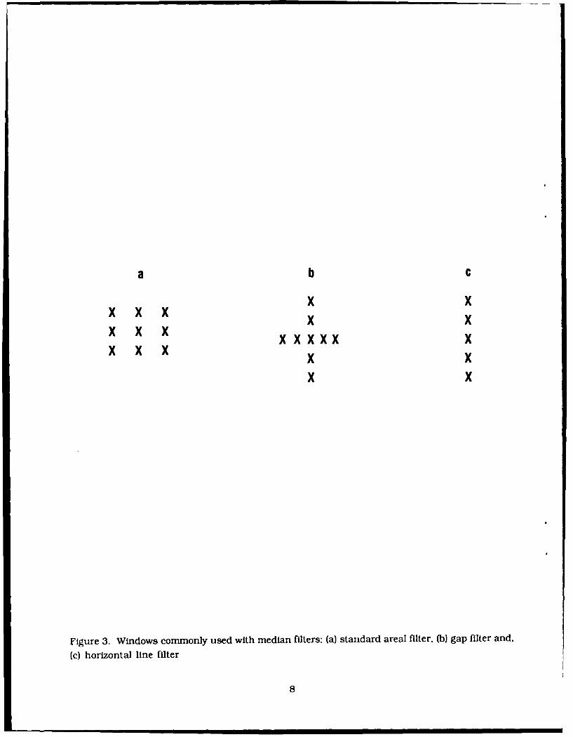
The first step in the processes of noise suppression and data smoothing is the application of amedian filter. The filter is of some specified geometric shape (window) with an odd number ofelements. The center data value within the window area is replaced by the median of all values in thewindow. The filter can be passed across the entire data field, sometimes as many as 2-3 times insuccession, to achieve the desired effect. Some more commonly used windows for a median filter areshown in Figure 3. The RAPID methodology employs the 3x3 box to remove noise spikes often seen inradar data and to smooth field intensity contours. The 1x5 line filter is used to eliminate missingscan lines often found in satellite imagery data.

Median filtering is highly effective for noise suppression. In general, regions that are unchangedafter a single pass of the median filter will remain unchanged in subsequent passes.6 With image dataquantized into various discrete levels, only contour edges will be affected by successive medianfiltering, since these areas are the only locations exhibiting field change. The effect of a simple 3x3filter is demonstrated in Figure 4.

A two-dimensional filter such as the 3x3 box filter generally preserves edges but removes thinlines, raggedness, and smoothes out corners. A plus-shaped filter generally preserves horizontal andvertical lines and comers but removes diagonally oriented lines and comers. Thus, small-scale(relative to the size of the filter) perturbations of a feature will be smoothed by a median filter.

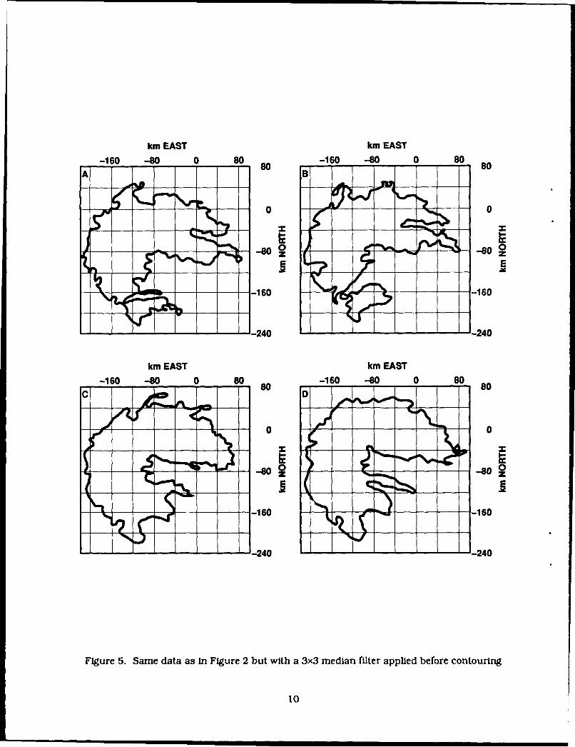
Figures 5a-d show the results of applying a 3x3 median filter to the composited data used togenerate Figures 2a-d. The filter eliminates the small scale raggedness along the contour, resulting in

6. Pratt, William K. (1978) DIgtal Image Processng, Wiley-Intersclence, New York.

6

km EAST km EAST

-160 ~ ~~~ -8 0 s 10 -s o 8 0 z

-80 8 0

E E

- - - - -- -1- 224

Figur 2.S The 32dZrfetvt otu opstdrfESTv ie sFgr

-160 -80 so so -60 W 0 0 7

a b c

x xx xx x xx x x xx x xx x

x x xx xx x

Filgure 3. Windows commnonly used with median filters: (a) standard areal filter, (b) gap filter and,

(c) horizontal line filter

8

C, LU

COD U.

CLu

C'4u

0zo *~- - '- 1

4')

x x

'caI- W

LUU

I---0 Y

0 0.

-A L cmcm D 9

km EAST km EAST-160 -80 0 so0 s -160 -80 0 80 8

80 80

2 ,

-. so- 0 - \. -- s - 0Ik-160 .- 16

-240 -4

km EAST km EAST

-160 -80 0 8 0 -180 0 80

Figure 5. Same data as in Figure 2 but with a 3x3 median filter applied before contouring

10

I II I I

a more conservative field. However, the contour structure in this particular example is still

considered more complex than can be effectively handled in current tracking and forecasting

schemes. This is an example where further applications of the filter are required.

One problem that arises with use of a median filter Is that its response function is basically

unknown. This is because the data value selected to replace the center value can be from any location

within the window area. Thus, there is quantitative uncertainty as to its effects upon the distribution

of small-scale features within the data. However, since the goal is to achieve a conservative field

contour and the filter does preserve the larger scale shape of the contours while smoothing the smaller

scale noise, the effects are considered, and have so far been observed, to be unimportant.

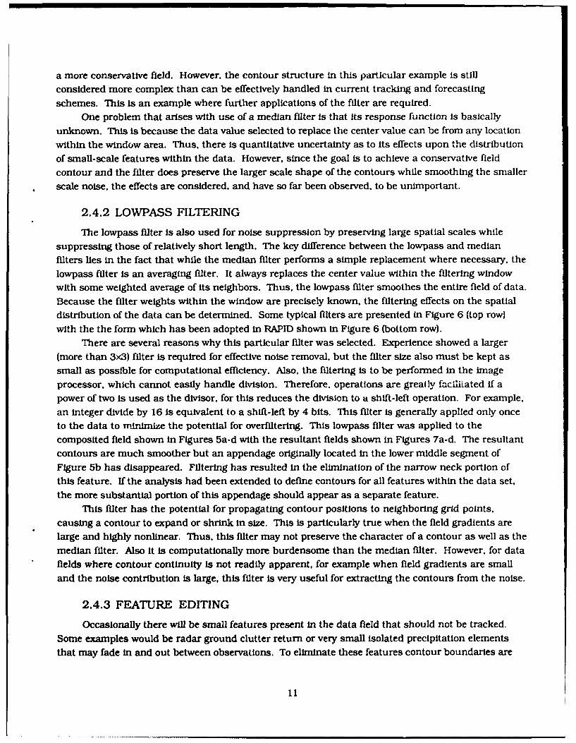
2.4.2 LOWPASS FILTERING

The lowpass filter is also used for noise suppression by vreserving large spatial scales while

suppressing those of relatively short length. The key difference between the lowpass and median

filters lies in the fact that while the median filter performs a simple replacement where necessary, the

lowpass filter is an averaging filter. It always replaces the center value within the filtering window

with some weighted average of its neighbors. Thus, the lowpass filter smoothes the entire field of data.

Because the filter weights within the window are precisely known, the filtering effects on the spatial

distribution of the data can be determined. Some typical filters are presented in Figure 6 (top row)

with the the form which has been adopted in RAPID shown in Figure 6 (bottom row).

There are several reasons why this particular filter was selected. Experience showed a larger

(more than 3x3) filter is required for effective noise removal, but the filter size also must be kept as

small as possible for computational efficiency. Also, the filtering is to be performed in the image

processor, which cannot easily handle division. Therefore, operations are greatly facilitated if a

power of two is used as the divisor, for this reduces the division to a shift-left operation. For example,

an integer divide by 16 Is equivalent to a shift-left by 4 bits. This filter is generally applied only once

to the data to minimize the potential for overfiltering. This lowpass filter was applied to the

composited field shown in Figures 5a-d with the resultant fields shown in Figures 7a-d. The resultant

contours are much smoother but an appendage originally located in the lower middle segment of

Figure 5b has disappeared. Filtering has resulted in the elimination of the narrow neck portion of

this feature. If the analysis had been extended to define contours for all features within the data set,

the more substantial portion of this appendage should appear as a separate feature.

This filter has the potential for propagating contour positions to neighboring grid points.

causing a contour to expand or shrink in size. This is particularly true when the field gradients arelarge and highly nonlinear. Thus, this filter may not preserve the character of a contour as well as the

median filter. Also it is computationally more burdensome than the median filter. However, for data

fields where contour continuity is not readily apparent, for example when field gradients are small

and the noise contribution is large, this filter is very useful for extracting the contours from the noise.

2.4.3 FEATURE EDITING

Occasionally there will be small features present in the data field that should not be tracked.

Some examples would be radar ground clutter return or very small isolated precipitation elements

that may fade in and out between observations. To eliminate these features contour boundaries are

11

ad.

0

10

cm C=

cm C2

V- COJ I-,-

4K)

(0

(0Cu

4K 4)o

I- 1~ Z

12

km EAST km EAST-160 -80 0 80 -160 -80 0 80

" I _fo 1

0 0EE

-- 160 - 16

-240 -240

km EAST km EAST-160 -80 0 80 -160 -80 0 80

80 80 0

E EL -- 160 -160

-240 -240

Figure 7. Same data as in Figure 2 but with both a 3x3 median and lowpass filter applied

before contouring

13

interrogated to determine their length (in pixels). If the boundary size of the region is smaller thansome predetermined value, then the region is considered to be a contaminant and is eliminated byreplacing it with the neighboring field mean value (or lower threshold value if the data are quantizedinto discrete threshold levels).

2.4.4 GAP FILLING

Missing data may be accounted for in a number of ways, the simplest being replacement with avalue determined from the neighboring data field. The gaps usually reside in low radar reflectivityfactor regions, typically along the storm boundaries or internal regions where the missing data areessentially surrounded by useful data. Care is taken to not extend storm boundaries unnecessarily, orto fill in regions where the radar did not scan completely (for example, near storm top). Typically, gapfilling requires minimal intervention and usually is performed during standard median or lowpassfiltering of the data during noise removal.

3. FEATURE MAPPING AND ATTRIBUTE DEFINITION

3.1 Feature Forecasting Considerations

The techniques developed here are generic in the sense that they may be applied to any two-dimensional field of data with distributed values. The methods have been tested on data from bothradar and satellite sensors. The initial intent was to merge satellite and radar data into a single datafield that would be useful for forecast generation. However, radar measures reflectivity factor fromthe precipitation throughout the storm volume while a satellite measures visible and infraredradiance from the cloud boundaries. Since there is no good physical relationship between these

measurements, numerical combination(s) of the three fields is really not possible. Qualitativemerging of the fields is possible if the data are composited in a binary fashion (that is, if grid value is

above a threshold value, the grid value is set to 1) or contours of the respective fields are overlaid.However, the magnitudes and spatial distributions of the individual fields are lost. Also, the temporal

resolution of the radar and satellite data are 5 - 7 min and 30 min, respectively. Neither overlaying anevolving radar data field on a stationary satellite field nor discarding radar data not coincident withsatellite data can be considered as reasonable approaches. Since many of the expected applicationsare affected primarily by precipitation rather than by cloud, and because satellite data are of little usefor the forecasting of rapidly evolving precipitation fields, primary emphasis was placed upon use of

radar data.There are two basic philosophies that may be adopted to derive forecasts of precipitation field

motion and evolution from the radar data. One is to perform correlation analyses over limited areas,until the entire data set has been interrogated. 7 . 8 These techniques work extremely well for tracking

7. Rinehart, RE. (1979) Internal Storm Motions from a Single Non-Doppler Weather Radar,NCAR/TR- 146+STR, National Center for Atmospheric Research, Boulder, CO. 262 pp.

8. Smythe, G.R. and Zrnic', D.S. (1983) Correlation analysis of Doppler radar data and retrieval ofthe horizontal wind. J. Clin. Appl. Meteor. 22:297-311.

14

precipitation features having scales of the order of 5 km. However, they are notoriously slow,9 evenwith limited data sets. Because the 0 to 30 min forecast problem requires utilization of every availableradar scan sequence, and each sequence may result in as many as three two-dimensional fields (threeselected altitudes) of data, with each field containing up to 256x256 grid points, correlation techniqueswould not support real-time operations and are not employed. However, this approach may bereconsidered for a 0 to 2 hr forecast effort to be addressed in a future task.

The second philosophy is to extract features from the data, determine their attributes, and

forecast changes of these attributes. These attributes might include such quantities as centroidpositions or storm boundaries. The intent here is to reduce the amount of data tracked and forecast,while still retaining an accurate description of the spatial distribution of the precipitation field. Thenormal mode of operation for an observer is to view the field of data and first locate features such asmaxima, minima, and gradient zones. That is, the observer mentally thresholds the data todetermine the spatial structure. This natural method of using thresholds to delineate areas of selectedintensity, with each such area identified as a feature, is employed in RAPID.

3.2 Data Representation Considerations

There are several ways one might represent the features and derive characteristics that couldthen be used for generating predictions. One approach is to utilize binary data values where gridpoints with values below the threshold are given a value of 0 and those above a value of 1. The result isa region(s) of is delineating the desired feature(s) surrounded by a field of Os. While this methodcertainly makes features easily identifiable, the resulting data set may still be large and requiresignificant computational time and power.

Another approach is to simply follow the contour of the feature, as defined by some thresholddata value, and retain only sufficient information to describe the contour. This approach thenreduces the two-dimensional intensity distribution to a set of user-selected contour lines. Theworking data set size is significantly reduced with the degree of reduction being dependent upon themethod used to describe the contour. Judicious selection of contour thresholds allows for adequatedescription of the data field. Because of the significant restrictions on computer mermory, andanalysis and forecast update time, this approach was chosen.

3.3 Contour Extraction

Three techniques were considered for extraction and description of the feature contours:specifically, use of interpolated Cartesian contours, geometric approximation methods, and theFreeman chain code. These will %e discussed in terms of their formulation and advantages.

9. Smythe, G.R. and Harris, F.I. (1984) Sub-Cloud Layer Motions from Radar Data UsingCorrelation Techniques, AFGL-TR-84-0272, AD A156477.

15

3.3.1 INTERPOLATED CARTESIAN CONTOUR AND GEOMETRICAPPROXIMATION

There are numerous methods that delineate contours by employing interpolation procedures toprecisely locate the coordinates of contour points. Generally the data are searched until a value is

found that exceeds the desired contour value, and the contour locations about this point are then

determined by interpolating between the current position value and data on neighboring grid points.

The interpolation filter can have a variety of forms such as uniform (average), exponential, and

Cressman. The number of points employed in the filter can be as few as four or as many as containedin the entire field. Obviously, the more complicated the filter and the more points used, the greater

will be the amount of time and memory required for data processing. This technique generally results

in the most accurate determination of the location of a contour, for it allows for interpolation betweengrid points. The resulting data set, a two-dimensional array of the contour coordinates, 1 0 are stored

for further processing. This technique is somewhat cumbersome and the interpolation procedure can

be time consuming if the contour is large and complex. Thus, it is not considered viable in the rapidupdate time frame considered here.

The second technique, geometric approximation, involves fitting a variety of sizes of specific

geometric figures such as ellipses to the feature. This technique has been used in forecasting synopticscale pressure patterns I I and heights of pressure surfaces. 12 The technique is especially suited tothese types of feature forecasts since representations of low and high pressure systems tend to be

somewhat elliptical with smoothly varying contours. Basically, the technique involves locating thecenters of all maxima (and minima for synoptic data) within the data set. Then with an adaptive

nonlinear, least-squares algorithm, 13 ellipses are fitted to the desired contour(s), one for each

maximum. The family of fitted contours are the equivalent representation of the original contour set.Five parameters of the ellipse are allowed to vary: the coordinates (2) of the center of the feature, thelength of the major axes, eccentricity, and orientation angle of the ellipse.

Generally, this technique has been used for features that are relatively conservative in nature,that is. those that evolve slowly between observations. Also the contours generally have simpleoverall shapes and vary smoothly. Unfortunately, as often observed from radar echoes there isusually a high degree of evolution in the precipitation patterns within storms and the contour shapes

are often complex. To make this method robust enough to accommodate these types of data would

require excessive field smoothing to force the contours to adhere to the constraints of simplicity and

slow change. Thus, although this method is attractive by allowing for significant data reduction, the

equivalent representation can be in error and thus this technique is not employed.

10. Dudani. S.A. (1976) Region extraction using boundary following, Pattern Recognition andArtificial Intelligence (C.H. Chen, editor), Academic Press, Inc., New York, NY, ,'p. 216-232.

11. Clodman, S. (1984) Application of automatic pattern methods in very-short-range forecasting.Proc. Nowcasttng II Symposium, Norrkoping, Sweden, ESA SP-208.

12. Williamson, D.L. and Temperton, C. (1981) Normal mode initialization for a multilevel grid-point model, Part It: Nonlinear Aspects. Mon. Wea. Rev. 109:744.

13. Dennis, J.E., Gay, D.M., and Welsch, R.E. (1977) An Adaptive Nonlinear Least-SquaresAlgorithm, Cornell Computer Science TR77-32 1.

16

3.3.2 FREEMAN CHAIN CODE

A simpler concept was introduced by Freeman. 14 As in the interpolated Cartesian contour

method, a threshold is applied to the data. However, for the Freeman technique one needs only to

determine whether grid point data values are above or below the threshold value. This effectively

reduces the data to binary form and makes the desired feature distinct from the background. The

contour of the feature is extracted and stored as a one-dimensional directional array, with each array

entry having only one of eight possible values.

To extract the boundary and form the directional array the two-dimensional data field is

scanned in a left-to-right, top-to-bottom manner until a point on the boundary of the contour islocated. This is referred to as the starting point, or origin, of the contour. Its (xy) position in the grid

is saved as the first element in the contour array. From this grid point the contour of the region is

determined by keeping the feature within the contour always to one side of the path being followed (for

example, to the left) while searching for the next nearest grid point on the contour. Once the next point

is found its location may be represented by the directional code presented in Figure 8. In this figure,

the x represents the original contour point and the numbers represent the direction code (angle) from

that point to the next contour point. Because the grid is regular, these eight directions (angles)

represent all the possibilities that one might encounter. Thus, one simply walks around the feature,

determining a directional code for each boundary point until the starting point is again encountered.

The codes leading to the nearest neighbors for all newly located boundary points are saved in an

array, along with the origin and final length of the code. Collectively, these three elements completely

describe the contour of any closed region and the two-dimensional data array has been reduced to the

one-dimensional representation of the Freeman chain code. 1 5

An example of the process is shown in Figure 9. The boundary of the rectangle is completely

described by:

1) the origin is (1,1)

2) the number of elements in the directional code array is 18

3) the directional code array is ( 3, 3, 3, 5, 5, 55, 5, 5, 7, 7, 71, 1.,1 , 1. .

Thus. a 28 point two-dimensional array (56 elements) has been reduced to a 19 element one-dimensional array. The relative reductions are obviously much more significant for larger features.

The Freeman chain code was adopted because it simplifies the working data set while still

retaining complete information of all contour characteristics. It can make subsequent processing

more manageable while still accurately representing the field of data. This fact is of considerable

importance for it directly affects the real-time capability of the forecasting program. The

precipitation field can vary from very simple stratiform with slowly evolving features to multicell

storm environments where the data fields are complex and can change significantly between

14. Freeman, H. (1961) On the encoding of arbitrary geometric configurations, IRE Trans. Electron.Comput., EC-10:260-269.

15. Wu, Li-De (1982) On the chain code of a line, IEEE Trans. Pat. Anal and Mach. InteL, PAMI-4(#3):347-353.

17

2 3 4

Figure 8. The eight direction vector codes used In the Freeman chain code representation

18

o I 2 3 4 5 6 7 8I I I I I I I I

* \N\\\\\\N\N\NNNN\N\\\\\NNN\\\\\NNN\\\\\NNN\\\\t\S\\\\\N\\\\\\\\\\\N\\\\\\\\\\N\\\\\\lI N\\\\\N\\\N\\\\\\\\NNN\\N\\\N\\\\\\\NN\J\\\\\\\\\\\\NNNN\\\\\\\N\\\\\\\\\\\\N\\\\\\\\

I\\S\N\\N\\N\\\\\\\\\\NN\ N\N\NN\N\\\\\NNNN\\\\\\3 N\\\N\\\\\\\\N\\\\\\\\N\N\\\\NNNN\\S x \ \ \ \ \ \ \ \ \ \ \\ N\ N\ * \ \ \ \ \ \ \ t N \ \ \ \ \ \ N \ N N NO\ \N\N\NNN\\\\\\\\N\\\N\N\\\\N\N\NNN\\\NIN\\\NN\\\\\\\\\\\\\\\\\\\\\\\\\\\\NNNNNN\\\N\

%N\\N N\\N\N\NN\\N\NN\N\\NN\NNNN\\\NNNN\\\\\NN\\NN\D • %\NN \N N N N N N N N N N NNNNN\\ \ \ \ \ \\ \ \ \ N\NNNNNNNNNNNNNN

1\\\\\NNNNN\\\!NNNNNNNN\NNNNNNNN\\NN\\\NNN\NNNNNNNN1

5[

Figure 9. A rectangular region of data with a contour boundary defined by the chain code(33, 3. 3,5. 5, 5. 5, 5 5 7, 7, 7. 1. 1. 1. 1. 1. 1). with origin (1. 1) and length 18

19

I NNNNNNNNNNNNNNNNNNNNNNNNNNNNNNNNNN

N

observations. Thus the methodology must be versatile while remaining representative. Furtherrestrictions imposed by the desire to store data and perform the bulk of the calculations within theADAGE image processor also support the use of this chain code representation. The versatility of theFreeman code will become more apparent in the following discussions of motion detection and

evolution.

4. FEATURE MOTION AND EVOLUTION

4.1 Introduction to Feature Monitoring

A number of methods for monitoring the contour changes over time were investigated. Use of the

chain code representation facilitates, but does not necessarily dictate, that simple analysistechniques will ensue. In fact, direct use of all chain code elements can result in a very complex and

time consuming effort. Use of techniques that employ the chain code to determine "attrlbutes" of thefeature and further reduce the amount of data monitored are required and arc illustrated in the

following sections.

4.2 Orthogonal Vector Method

One of the first algorithms exariined for mapping motions of contour points between successiveobservations involves the use of vectors orthogonal to the contours. For each grid point along acontour, the two neighboring chain code directions are combined to determine a resultant orthogonalvector direction. Once vector directions for all points along the contour have been determined, thecontour Is then aligned with the same contour at the next observation time (for example, by means ofminimizing the areal difference between the two contours or by overlaying the areal centers).Orthogonal vectors are then extended from the first contour until they intersect the second. With theassumption that the intersection points are the new positions of the points from the original contour,the contour point displacements and thus complete contour change between observations, isdetermined.

An example of this technique is plotted in Figure 10. Quite obviously there are regions where thistechnique fails miserably. Where the contours are straight or strictly convex it is quite effective.However, where significant concavity or small irregularities are present many intersecting vectorsare produced, resulting in obviously erroneous contour point displacements. Averaging or thinning ofthe orthogonal vectors to generate smoother contours or fewer contour points tends to alleviate, butnot eliminate, this problem of crossover. Objectively untangling these vectors, although possible,appears too complex for real-time analysis. Thus, this technique is considered unacceptable for thecurrent problem, but may be utilized in later efforts where highly smoothed data fields may beemployed.

4.3 Contour Segment Matching

Examination of the contours in Figures 7a-d indicates that there is reasonable temporalcontinuity between the contours. This suggests the possibility of matching contours from one

20

-30° -20 -10 0 10 20 30 4- - - -45

____ _ _ ___--35

-5

Figure 10. An example of the Orthogonal Vector Technique. Contours are of Infrared temperaturefor two scans 30 mln apart. The heavy contour Is for the earlier data. The orthogonal vectors areshown as short dashes

21

observation to the next. Methods employing the overlaying of two successive contours and movingthem about until the areal overlap difference is minimized or collocating the centers of areas of thetwo contours are useful if the fields are evolving slowly. However, rapid evolution or differentialmotion of the contours easily disables these schemes. It Is more reasonable to break up the contoursinto segments and then find the best matches between segments of successive contours. This methodallows for monitoring the preferential growth, decay, and advection of contour segments.

Two techniques were explored for boundary segment matching:(1) Finding the best match of straight line segments

(2) Performing a least squares fit of fixed length contour segmentsBoth techniques were implemented and are discussed in the next section.

4.3.1 MATCHING STRAIGHT LINE SEGMENTS

A means of classification is utilized to segment a contour chain code into a sequence of straight,or pseudo-straight, lines. Quite obviously, when working with pixel data (Cartesian data) only thoselines oriented parallel to one of the axes is truly straight. Lines canted at some angle (pseudo-straight)are somewhat distorted, being composed of chain code vectors that oscillate about the mean direction.However, they can be conceptually approximated by a straight line through the mean positions. In thediscussions that follow, reference to straight lines also refers to pseudo-straight lines.

The Freeman criteria for a chain code segment to be a straight line are:

(1) at most, two basic directions are present and these can only differ by 1, modulo 8.

(2) one of these values always occurs singly.

(3) successive occurrences of the principal direction occurring singly are as uniformly spaced aspossible.

Application of all three criteria in the operational arena is overly restrictive and results in amultitude of very short line segments that become difficult to track between observations. Therefore,conditions were relaxed by invoking only the first criterion. This reduces the number ofcomputations, tends to decrease the total number of segments, and accordingly increases the size ofsome segments.

Beginning with the first chain code element the subsequent codes are surveyed so as to find thelongest segment including that first element that conforms to the definition of a straight line. Onceidentified, the beginning segment number, length, and primary direction of the line are recorded. Thisprocess Is done iteratively, each new starting point being the first contour point after the end of thepreviously determined line segment. When the absolute starting point is included in a line segmentthe last line segment has been determined and the segmentation process stops. For example, thedirectional code for the box in Figure 9 is given by

C= 3,3,3, 5,5, 5,5,5.57, 7,7, 1, ,1 1, 1, 1

The maximum line lengths for each direction can be easily identified here and are shown in Table 1.In real situations, there are many more straight line segments, each identified by their direction code,length in terms of number of direction codes in the line, and the starting position of the line relative toits !ocation from the absolute beginning of the contour chain code. The listing shown in Table I Is in

22

p

-00

Lu

Lu

z

C.)

LU

I0 IDxLm In Lo~ C2 CV

Lu z

COO)

L Z

LU3

the order determined by the straight-line algorithm which ranks first by length and second by

absolute segment starting location.

Now assume that the feature observed in Figure 9 was observed later (Figure 11) with the

resultant chain code:

C=3,3,3,5. 5, 5, 5, 6.6.6, 1, 1. 1, 1 1, 1

The results from the straight-line analysis are also included in Table 1. Due to evolution, the results

for the two examples are somewhat different. With the straight line segments for a given contour

identified for two successive data fields, the process of matching segments between observations is

begunIt must be noted that a contour is continuous and the starting location is basically arbitrary. In

the example here, the upper-left-most pixel is defined as the origin, but it could just as well have been

the lower-right-most. Therefore, the code and associated data are treated not as an ordered linear list,

but in a circular fashion, for example, a circular queue, Since the chain code is a directional code the

shape and orientation of the contour are always preserved, independent of the absolute starting

location of the contour code.

The rule hierarchy that has shown the greatest success is:

(1) Search for the longest segments in each contour and match the segments that have the same

code.

(2) Proceed iteratively with successively shorter segments until no more matches can be made.

(3) For those remaining line segments attempt to find approximate matches by comparing

starting locations.

For the simple examples of Table 1, the matchups would be line 1 to 2, line 2 to 1, line 3 to 3 and line 4

to 4.

4.3.2 CURVE FITTING CHAIN CODE SEGMENTS

The second approach in curve fitting is to break down the contour chain code into segments

having a fixed number of elements regardless of chain code values. This technique focuses on

matching similar shapes, a method of pattern recognition. While the straight-line segment approach

adopts the simple technique of matching segment lengths and code values, here a more complex

procedure is required: namely, least-squares fitting of the chain code directions between segments in

successive observations. The underlying assumption is that between observations the processes of

advection and evolution still allow contour segments to retain their overall shapes. The chain code ofthe selected contour is divided into segments of specified length, usually 10 to 25 percent of the total

number of codes in the chain. Each one of these segments is then compared with every possible

segment of identical length in the contour chain code set of the next observation. For eachcomparison, the mean difference and the mean square of the differences of the individual chain codedirections are computed regardless of location along the contour. A perfect match is obtained when

the mean difference is zero and the mean square of the differences is a minimum.

An example of this process is shown in Figure 12 where these two parameters are plotted againststalling segment number for the second contour. There is a very obvious minimum of the mean

24

0 0 0

0 *k N NZ T '7

*5E ~\~ \\\\t<~NKK\\\\

Figure N 11 Evlvng rtn gua cotu ofN Figure 9 bevdaaltrtm

NN NN N NN 25N

I--

w w

w w D

w 0

a c

Lu C

C-

z 00

0I w

crz v4.0

cr--to C'J

(sun G3NIH) 3J~JI U.O NV0 4OO(siI~~~~n 300NVO 0N0JI V~

26~

squares of the differences at segment position 308 along with a near zero of the mean difference. Thiscombination represents the best match for this case. Note that the crossover of the mean differencecurve from negative to positive near segment location 175 occurs with a maximum of mean squaredifference, and thus is not a good match. Not all attempts at curve matching produce such pleasingresults, particularly where there is considerable evolution between observations. However, in allcases where the fit looks reasonable to the eye, the best fit Is usually identified with the minimummean square difference. Thus, the resulting matching criteria are a near minimum mean square

combined with a relatively small mean difference.

4.4 Attribute Determination and Evolution Detection

Both the straight line and curve fitting algorithms perform mapping between segments ofcontours from successive observations. Each segment has several associated characteristics;including a segment length, orientation, starting point value, and distance from some point ofreference to a given point in the segment. This limited set of quantities completely describe thecontour segments and are termed the segment "attributes". If there is reasonable continuity betweensuccessive contour observations, that is, if segment matching between the contours may beaccomplished, then one has a mechanism for monitoring the evolution and motion of contoursegments and ultimately the contours themselves. Through use of relatively simple techniques, thetwo-dimensional data fields can be described in terms of selected contours. These contours can besubdivided into contour segments, which can then be described in terms of segment attributes. It isonly necessary to monitor and forecast attributes to develop forecasts of future cloud andprecipitation field distributions. Thus, it is segment attribute histories that will serve as input to theforecasting algorithms.

5. FORECASTING

5.1 Forecasting Considerations

A number of restrictions are imposed upon the forecasting process. First, the desire to develop

forecasts in real-time demands techniques that run quickly and efficiently. Second, the frequentlyshort lifetimes of some storms require that forecasts be developed from limited data histories. Third.the desire to store all necessary historical data and perform the bulk of the data processing within theimage processor demands use of analysis techniques that minimize data storage requirements.Computer memory and time constraints also demand that the number of quantities input to theforecasting process be as small as possible, while still adequately defining the evolving nature of thestorm precipitation intensity contours. These considerations have profoundly influenced thedevelopment of both the data storage and forecasting methods.

These considerations, as previously discussed, have led to tracking and forecasting a highlyreduced set of variables termed contour attributes. These have been identified to include such items asline length, location, and orientation, and chain segment orientation and location. Forecasting theevolution of a contour thus requires monitoring these attribute values for all contour segments.

27

developing the historical attribute data sets. forecasting the future attribute values, andreconstructing and linking the forecast contour chain code segments.

The attributes being followed and forecast are not standard meteorological quantities, but rathera very limited set of arbitrarily defined variables. The forecasting process may thus be approachedfrom a nonmeteorological orientation, at least in the sense that (1) there is no physical model forproviding a priori expectation of the behavior of the attributes and (2) attribute variations may noteasily be linked to other observations of the physical environment. It is assumed that time variationlies somewhere between a state of stationarity to perhaps quadratic variation. For example, if the linelength or orientation for a contour segment were stationary, then Its value would remain constantduring observations. If a linear variation were observed in line length of a non-rotating line, then thetotal number of code elements composing the line would be increasing or decreasing by a constant ratebetween observations. This assumption can be severely strained during periods of rapid stormdevelopment where production of new cloud and precipitation may occur on the order of minutes.However, rapidly evolving storm environments where only a very limited number of observations areavailable make estimation of more complex time trends (for example, quadratic) grossly inaccurate.Thus, the assumption is made that the attributes are random quantities, a combination of somequasi-linear trend variation and noise.

The forecasting process has focused on extrapolation routines that employ smoothing functions.These routines either explicitly or implicitly employ knowledge of past attribute variation. Someprovide for user-selected preferential weighting of current or past observations, or automaticadaptation to the changing environment through monitoring forecast errors. The routines alsoperform automatic filtering of noise contributions. Finally, they are hig r efficient, requiring onlya very limited amount of input information and computer operations to generate new forecast values.The following material will address some relevant features of these classes of routines and presentsome observations of their utility and deficiencies, leading to the selection of preferred forecastingalgorithms.

5.2 Forecasting Techniques

5.2.1 TECHNIQUE FORMULATIONS

A total of nine forecasting techniques were considered, providing an overall capability forassimilating data ranging from stationary to quadratic behavior. The routines are listed in order ofcomputational complexity in Table 2. and the generic formulations describing them are presented inTable 3. Before discussing their performance with data, It is instructive to develop a clearerunderstanding of the characteristics of these classes of routines.

The stationary formulations, as indicated in Tables 2 and 3. inherently assume the variablebeing forecast is statistically stationary (for example, in time), perhaps a combination of a constantmean value with an added random component. The Simple Moving Average (SIMMOVAV) method is amoving box filter, using the average of the latest three observations as the forecast value. The SimpleExponential Filter (SIMEXP) method develops a forecast from a weighted sum of the currentobservation and the previous forecast for the current time and employs a user-selected constantweighting factor allowing for preferential weighting of the two terms. The Adaptive Simple

28

'u

oot- CD~ 0 C 4 c.J

L..

UL

.0

zU C-2 CoCDc C ,l= C4 U 4

00

00 0 -

W-JL

LLU- ~ L m ~ 2L~ 0

Q) P : ccLU 4 A4C LU C CCO 2 Z CDC%

4cc C2

c~i 0C34)cc mIi EE

cr- 29

00

UU

0

V

UU

zc0+

x 0

Cui

0 +I Ulmp

U~C ccS .

cc ~ cc

+ P+

u. w

C6~

4))10 SI

- -

o3

Exponential (ADSIMEXP) method uses the same formulation as SIMEXP but it alluws the relativeweighting of current and historical data to adjust automatically with each new observation. Thisweighting factor is determined from the ratio of total forecast error to total absolute forecast error,where error is defined as the difference between the past forecast for the current time and the current

observation (error = F(t) - X(t)). Since the numerator (total error) may fluctuate between positive andnegative values, and the denominator (total absolute error) continually increases, the magnitude of

the weight decreases with increasing time. Thus the asymptotic trend is for diminishing dependenceupon current observations and growing dependence upon the historical mean value. As more data areacquired the historical mean will approach the population mean (if observations are in fact a sum ofmean and noise terms). The Modified Kalman (KALMAN) filter works similarly to the standardKalman filters except that it employs only the latest three observations and forecasts in determining

the new weights. In this modified form the automatically adjusting weight applied to the currentobservation is equal to the variance of the last three forecasts, divided by the sum of the last threevariances of the observations and forecasts.

While the SIMMOVAV (moving box filter) method employs only the latest three observations inderiving a new forecast, the SIMEXP, ADSIMEXP, and KALMAN methods implicitly utilize the currentand all previous observations, however, old observations become increasingly less important as newobservations are acquired. This dependence upon historical data can be easily shown for the SIMEXP

method:

F(t) = A*X(t) + (I-A)*F(t)

= A*X(t) + (1-A)*(AX(t-1) + (1-A)*F(t-1)).

= A*X(t) + A*(1-A)*X(t-I) + ... A*(1-A)**(N-I)*X(t-N-1)

Except for SIMMOVAV the underlying concept remains the same, namely: (1) the forecasts areweighted sums of all observations; and (2) recent observations are weighted more heavily than old

observations.

The nonstatlonary formulations tested fit either a linear trend or quadratic variation to thedata. The Linear Moving Average (LINMOVAV) filter employs two quantities: (1) a weighted mean ofthe past N observations (MEANOBS(N) = (obs(1) + obs(2) +...obs(N))/N) , and (2) a similarly weightedmean of the past N mean values (MEAN = MEANOBS(1) + MEANOBS(2) + ... MEANOBS(N))/N). Thelinear Adaptive 1-Parameter Brown (BWN1PAD) method revises both the origin and slope parameters

through use of a correction factor determined from the difference between the previous forecast andthe current observation. The linear Holt 2-Parameter (HOLT2P) method performs two smoothingoperations and revises the origin and slope terms independently with differing user-selected weights.The Linear Regression (LINREG) method is of standard form. It explicitly weights all data equally.Current data storage requirements restrict this technique to a maximum of the ten most recentobservations. The Brown Quadratic Exponential (BWNQUAD) formulation employs three averagingactions with a single user-selected weighting factor: namely (1) the average of the observations; (2) theaverage of the mean observations; and (3) the average of the average of the mean observation.

Although it appears somewhat convoluted, this method provides a relatively simple way of estin ting

31

first and second order trends, while at the same time filtering out random noise contributions. Except

for the LINMOVAV routine, these methods also employ all historical data.

5.2.2 TECHNIQUE INITIALIZATION AND USER OPTIONS

Since these routines are designed to employ a number of observations in deriving any individual

forecast, they generally cannot be "turned on" with acquisition of the first or second observation.

Rather, the routines employ initialization procedures that allow for gentration of forecasts throughuse of alternative and simpler methods until sufficient data are acquired to run the exact

formulations. These initialization procedures and the time delays before the first forecasts are

available through use of the exact formulations are presented in Table 4.

In initializing the stationary techniques it is assumed that the first observation is a good

estimate of the population mean and that it can be used as a first guess forecast. Thus, use of the

stationary data routines allows one to develop a forecast after the first observation. Use of

"difference" data. which are the differences between successive observations, delays the forecastingprocess by one observation period. As a result, the first forecast is obtained with acquisition of the

first "difference" data measurement, or second data observation. The time to pass through the

initialization stage and enter the true formulation varies between routines. For example theSIMMOVAV routine, which performs a running average of the latest three observations, does not

employ the exact formulation until the third observation period. On the other hand, the SIMEXProutine, which employs the current observation and the previous forecast, engages the exact

formulation with acquisition of the second observation. To initialize the nonstationary dataroutines, it is assumed that the first two observations represent a good first estimate of any linear

trend present in the data. The various initialization procedures may obviously be suspect in

environments where rapid evolution is underway, or where the observations include significant noise

contributions. However, the lifetimes of some meteorological events can be quite short andinitialization Is necessary for rapid forecasting of future attribute values.

The delay before entry into the exact formulation can be controlled for some techniques (forexample, SIMMOVAV, KALMAN. LINMOVAV) through selection of the number of entries utilized in theexact formulation. The requirement that routines be responsive to new trends in the data translates

to the employment of only a limited number of the most recent observations. Two observations

provide an estimate of change in an attribute value. However, if the noise contributes significantly tothe observed change, then forecasts employing trend estimation tend to be in great error. A greater

number of observations provide additional stability in the trend estimation process. Thecombination of potentially short feature lifetimes and the desire to develop forecasts quickly resulted

in the selection of three data values to drive the exact formulations where user-selection is allowed.The selection of optimum weights for the various routines is determined through observation of

their performance in differing data environments. One would expect an advantage in using adaptive

methods where the weights are adjusted automatically. with the adjustment generally being dependentupon the error between the observed and forecast values. The nine routines were evaluated on a seriesof test data, both simulated and real, to characterize their behavior and ascertain the optimum weight

values.

32

CID 0 00000 0

0 r,E E E

LU uj m C Mv~E 00 C,3 CL CO

0 Z -0 -+ + -

.0 .0. 0 C0 +CJ + +Cj

C.) 0), S -s

o :3. .

00

0 ~0.4-..

LuJ

0 0

U)Uc LU =I CL = C =00n 007C CD CL LCJ4

0. CD 4.c

re M7.. 0- c

.~CDCM Zi= - S

z

33

5.3 Forecast Technique Evaluation with Test Data

5.3.1 GENERATED TEST DATA

A small number of simple, but illustrative, data sets were generated for testing the forecastingroutines. The three data sets, as shown in Figure 13, consist of: (1) a constant mean with oscillation

about the mean: (2) a pure linear trend; and (3) a pure quadratic trend. A real-world scenario wasassumed where only a limited number of observations were made available to the routines. Althoughthese data did not allow for the effects of random noise, the relative performancc of the methods In the

controlled forecasting environment provide insight into the effects of initialization and their generalresponse. Figure 13a is representative of data having constant mean, but with an added error

(oscfllation) component. Two data sets are shown, one starting at zero, and the second starting belowzero. The second set was employed primarily to observe the behavior of nonstationary data routineswhen the initial data erroneously suggested a trend was present in the overall data set. Figure 13b

shows the purely linear data set and Figure 13c the purely quadratic.A number of factors were considered in comparing the relative performance of the various

routines, including: (1) actual forecast error; (2) total accumulated forecast error; (3) total absolute

forecast error, and (4) rate of response to changes in data character. These quantities were determinedfor one-interval, two-interval, and three-interval forecasts. An interval is the time between the start

of two successive observation sequences. Assuming new observations are acquired every 8-10minutes, this would produce the desired forecast warning times of 0 - 0.5 hr. Discussions will first

focus on stationary routines, then later be directed towards nonstationary routines. For thosemethods where user-selected weighting was available the three weights 0.3, 0.5, and 0.7 were employed.The plots shown will present the results from the cases which exhibited minimum error.

Samples of actual forecast error obtained with stationary data routines are presented in Figures14a-c. The range of actual error incurred generally lies between +/-0.2, comparable to the variation of

the input data about the population mean. The initialization procedures all allow a first forecast to begenerated with the first observation and the first measure of forecast error is obtained with the second

observation. Since all the stationary data routines are initialized similarly, they all produce the

same first forecast and incur the same initial error. Differences between routines become apparentwith the third observation, when the exact formulations are in force. These results indicate that allroutines perform quite similarly, the only significant exception being ADSIMEXP which responds

more quickly to input data variation than the other stationary routines. ADSIMEXP was found tooverreact to data variation with all test data sets. The oscillation in forecast error simply reflects

forecasted values that also oscillate, but which lag the input data sequence. The KALMAN methodshows negative (< 0) bias indicating the forecast underestimate Is greater than the magnitude of itsoverestimate. The other routines produce forecast underestimates and overestimates of nearly equal

magnitude.

The accumulated forecast error is useful for indicating the presence of biases in the forecasts and

are shown in Figures 15a-c for the stationary routines. The initial positive (> 0) biases result from thefirst observation being greater than the second, causing forecast overestimates. The error values

oscillate about zero and show no particular trends except for the KALMAN method, which has a trendtowards larger negative values. The results for the second data set (start below zero) are very similar tothose shown here, except that the accumulated errors are all displaced downward by about 0.4. This

34

stationary case

1.3

1 .2 ./ \/

,

/A

e 1.1 \

.,_ 1 .0

-~0.9/

\*\, /. \ /

0 .8 V

0.7

CU M - O r- O )

0 .6 '''''''

observat i on number

Figure 13a. Generated test case data for evaluating forecasting routines: stationary data with zero(dashed) and negative (solid) starting values

35

linear case9.0

8.0

7.0

- 6.0

_ 5.0

~4.0O

3.0

2.0

1.0

0.0 L) (0aC~jM U-) UD r--J CO P 1:

observation number

Figure 13b. Generated test case data for evaluating forecasting routines: pure linear

36

quadratic case90.0

80.0

70.0

4-,60.0

4,50.0

S40.0

30.0

20.0

10.0

0.0i

observation number

Figure 13c. Generated test case data for evaluating forecasting routines: pure quadratic cases

37

forecast I

.60

.40

C_ doC3 20C_C-W ,

.-I .00

4 -. 20

-. 40

-. 60

-. 80 ''''

observation number

Figure 14a. Plots of actual forecast error for SIMEXP (dash), ADSIMEXP (dash-dot),

SIMMOVAV Olong/short dash), KALMAN (solid) routines using stationary data (zero start) for

one-interval forecasts

38

forecast 2

.60

.40 /

0 20 /- ,C-

, .00

- .20 •

-.40

-.60

-.801

observation number

Figure 14b. Plots of actual forecast error for SIMEXP (dash), ADSIMEXP (dash-dot),

SIMMOVAV (long/short dash), KALMAN (solid) routines using stationary data (zero start) for

two-interval forecasts

39

forecast 3.60

.40

C._ -. 20 _C_

.40

-. 60 -

.80'.C__I CU M U) LO rC

observation number

Figure 14c. Plots of actual forecast error for SIMEXP (dash). ADSIMEXP (dash-dot),

'-IMMOVAV (long/short dash), KALMAN (solid) routines using stationary data (zero start) for

three-interval forecasts

40

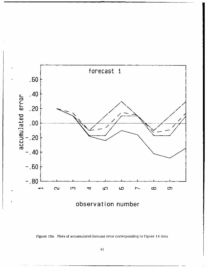
forecast I..60

c_ .40

C3L)(C

.20

CU M' U-) 0O)_ O C

* observation number

Figure 15a. Plots of accumulated forecast error corresponding to Figure 14 data

41

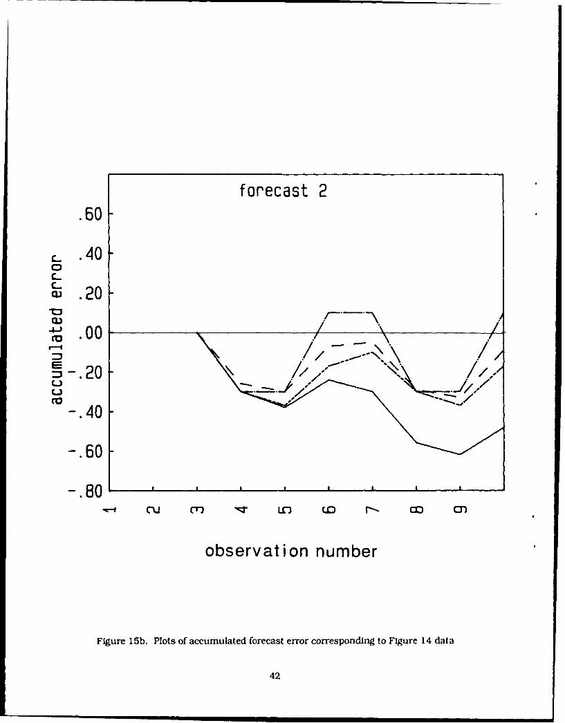
forecast 2.60

c .40C-4-CU .20

= -. 20 " ;

-. 40

-.60

-.80 1 r ' ' ', - '

observation number

Figure 15b. Plots of accumulated forecast error corresponding to Figure 14 data

42

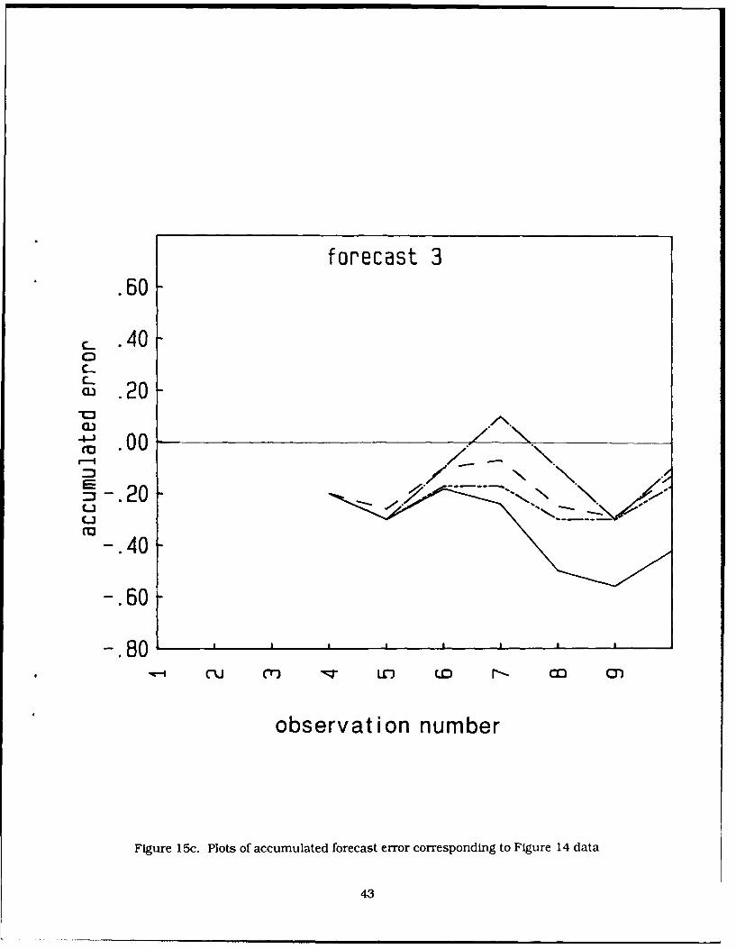
forecast 3.60

c- .40C-CU 20 N.

CU

4-1 .7-.. -.20

C-- .1"

-.40

-.60 -

-.80''''''' '*CU CO U-) LOC-C

observation number

Figure 15c. Plots of accumulated forecast error corresponding to Figure 14 data

43

reflects the first three forecast errors being negative in value, or the generation of forecast

underestimates.

The accumulated absolute forecast error provides a good basis for technique comparison and

results are presented in Table 5. It should be noted that the range of input data values for the

stationary test data is very small in comparison to the ranges encountered in the nonlinear test data

and that forecast error should be expected to increase due both to the data range and degree of

nonstationarity. In these comparisons, of interest are: (1) the response of individual routines to

variation of weighting factors and data type: and (2) the relative performance between the techniques.

Results from use of the stationary routines on stationary input data indicate that all perform

quite similarly. with slight preference given to the KALMAN method. The SIMEXP forecast error

increases with increasing weight applied to the new observations, indicating that the historical mean

is a better approximation to the population mean than the individual observations. This is certainly

an accurate observation for this particular data set. When the forecast is derived primarily from the

historical average the forecast relies upon a quantity which increasingly approximates the true

population mean as the noise effects are filtered out. The trend of decreasing total error for a given

routine from the one to three interval forecasts primarily reflects the smaller number of forecast

errors contributing to this sum for the larger interval forecasts.

These stationary routines behave quite differently when linear and quadratic test data are

introduced. The ADSIMEXP filter appears to be most accurate, reflecting the automatic adaptation of

the weighting factor. The best SIMEXP filter performance is obtained with the largest weight applied

to the new observations, reflecting better adjustment to the changing nature of new data and reduction

of the influence of the historical average. The KALMAN filter, on the other hand, senses less variation

among its forecast values than in the input data set and reduces the weight given to new input data

while increasing the weight applied to the historical data. This causes the KALMAN method to spiral

into a state of larger and larger forecast error. These initial results suggested that the ADSIMEXP and

SIMEXP (weight = 0.7) routines are the preferred stationary techniques.

The nonstationary techniques may be similarly compared. With stationary input data the

methods are all generally similar in response to the stationary routines except they incur slightly

greaLer error due to the attempt to fit linear trends to the data. This is particularly true for the first

one-, two-, and three-interval forecasts, as shown for the LINREG method in Figure 16. With no

historic& data to rely upon, LIN REG projects the trends observed from the first two data values into

the future. The box filter approach of LINREG method offers slightly better performance. This resilts

from averaging equally all available data from the periodic data source. With linearly varying input

data, all linear trend methods naturally return zero error. The BWNQUAD routine, optimized for

quadratic input data, employs a linear trend initialization scheme and suffers the greatest error

among the nonstationary formulations. Even so, this error is still not significant when compared to

the range of input data values, and all these techniques may be gauged satisfactory on stationary and

linear test data.

Significant differences between routine performance are observed when quadratic test data are

employed. The beneficial effect of preferential weighting of new input data (for example, increasing

weight for HOLT2P and BWNQUAD, decreasing weight for BWNIPAD) is easily observed. These

tecbniques have better absolute accuracy and show a greater relative increase in forecast accuracy

than possible with the stationary SIMEXP routine with large preferential weight to new data. While

44

(%J 04 U to U to C)to~- C14 CD n( C4)

* C i- t) Cl mo c'O r-

7-J T-- M m

too CZ ,'~ 7 *j to C~ - iC i cv a

0z CY! p C%! Cl ) CY! U-

i- e.M 4. r- mo c~o - 04 c D r

to C%i U

C.. U13 co i-C) c~j c o r.- C-4j C)

ecj C%j C) C7 C4J C.L CD Cka m~ 4= to

C-i~1' C-4 C= CI04 C

C= (mC1 C%Cl C., CN)C

7)l to

j to r- o =o C=. 0zC4 a

,..,o m- =P. V- C'.10 w)7

C C 0 N C") C--) 6 viJ C') C")

7-J C4 Go C J- CDJ 1 0L U2 =

U) 0 cm C..,='0en U)

CD)cctoC) . - ;t. to .O A o

U- j too LO LU toLOL

L.. .CO).

00

0" Ft, 00Z MC% to 0 0 CD CD to r--C013 0 Q ~

v rl C7! C") C")R i C U :

'U C" = =-C) t r- to )o

C0 - CD cc CD M C". -Cd,04

4) LO too CD C. wto CD C" C" 4 to f

0L U -- - ci C6 c C6! C'

x- 7- CM., " 04 to

7-C M C") R C) C C ."o4 ~- Cs, f ncz Lo

to4 to4 (0C) .0 m~ Owto 7- to . C14 04C t

D <- to C5 , 4 C ". C<, t

C") LI C") LL ccO i- -C) 0" 0L to to J <CL 'I- -3 214r- -:1,P E 0 Z PE

z O) -. cm cs* to cj 0 4a) i

C3.

B ~~~0

45~

forecast 1/2/3.60

.40 -

0 .20C- /C_

r .00 / /

-.202 7/-.40 - /

/-.60 //-.80

CI nC .0 rl- Go~ 0)

observation number

Figure 16. Plot of forecast error for LINREG method using stationary data (zero start) for one(dash), two (dash-dot), and three-interval (solid) forecasts

46

the SIMEXP method does adjust to a new "mean" it only projects Into the future the current mean

value.

Before wholehearted acceptance is given to any routine, other factors need to be considered.

Consider the variation of actual forecast error with observation number for the BWNQUAD routine for

the two cases of linear and quadratic input data as shown in Figures 17 and 18. The rapid decrease of

forecast error magnitude shows that the method adjusts to the true trend if given a long enough

historical data series and that most error occurs during the initial operation of the routine. This

routine performs three recursive smoothing operations. For the first filter, three observations satisfy

the data requirements where an average of the latest three observations is taken. However, the other

two filter operations operate on insufficient data. Five observations are actually required to engage

the true formulation to develop the first forecast. Thus this technique would appear most useful only

for features that may be tracked for long periods of time and for which forecasts are not required

quickly after first observation. This, however, does not address well the problem encountered here. A

tradeoff must be made between deriving forecasts early without the use of an extensive data base and

the desire to use the exact formulation.

Also, why not extend the usefulness of routines by employing "difference" data? This is

particularly attractive for the stationary methods due to their computational simplicity. The results

from use of such data are displayed in Table 6 and show the stationary methods can be effective for

original data having well-behaved linear trends. Use of "differenced" data derived from the test

stationary data results in slightly greater forecast errors since only noise serves as input to the

routines. The relative ranking of the routines remains unchanged with the ADSIMEXP and SIMEXP

methods being the most responsive of the stationary data methods.

Use of "differenced" data with the nonstationary routines results in unacceptable errors when

applied to stationary data but results n improved forecasts for original nonstationary observations.

The nonlinear methods all provide precise forecasts with the differenced data, although the

BWNQUAD method again has slight error due to the differing assumptions employed in the

initialization procedure and exact algorithm. There is little distinction between forecast capability of

nonstationary data routines when applied to "difference" data.

These results provide some initial insight into selection of preferred routines. The generated test

data suggested using the BWNQUAD (weight = 0.7) method for overall use if the features would be long

lived. Alternatively, input data comprised of difference data could be used with a variety of methods,

with preference given to LINREG, HOLT2P (weight = 0.5). BWNIPAD (weight = -0.5) and the LINMOVAV

routines. If the data were known to be essentially stationary in overall character, then the stationary

routines ADSIMEXP and SIMEXP (weight = 0.7) would appear most appropriate.

5.3.2 REAL TEST DATA

Control data brought some Insight into the mechanics and performance of the various routines.

Another test data set, obtained from satellite and radar observations of Hurricane Gloria was also

utilized. One data set, determined from GOES satellite IR imagery, consisted of the locations (XY) of

the center of area (COA) of the high cirrus shield (here termed cold dome) associated with the

hurricane. A second data set consisted of COA positions of hurricane rainbands as determined from

weather radar precipitation intensity contours. The results were somewhat unexpected. They

47

linear data

3.5

3.0

_2.5C-

_ 2.0

S1.5

1.0

0.5 .

0 .0 ;'- - -- ' -' -

observation number

-Figure 17. Plot of forecast error for BWNQUAD routine using linear data for one (dash), two (dash-

dot), and three-interval (solid) forecasts

48

quadratic data

1.0

0.0_

-1 .0 -

.......

C /c -2.0 -C-

-- 3.0

ro

-5.0

-6.0

-7.0

-8.0 ' p p p

observation number

Figure 18. Plot of forecast error for RWNQUAD routine using quadratic data for one (dash), two(dash-dot), and three-interval (solid) forecasts

49

902 c'2 CD C i m - C w LO

qeM CD CM LO I .-- F- CM t-

.JN' cM N N N) Ifl V mt r

CV)a 7- T- T. V V) C - V5 mv en C

02 V- CD C cc CM CD, co Cv, =v C2

r- Ci 00 CO U) 0 0: C CO 0

Si~~~C 04 0- CD C*c L02CDg0- oC

u. 12 Nm Le 0 0 CD Cv2 0V m C) cm

CLJ.. MR C00 to 1 m 0 2 0o mf CD 2

W! CM CM CDO CD wi0 0- ci

< (n 00 CR) R 0c Le Cv) c

UU COcc W

C N Nl c0c)C'

a-- L) cc0 co cm0 0

0v N 0.Os 0

4- 0: 0z w V- to cmz to ~ CV C )-WCzo

dc C.3 (

NM CC. RPI C CoR Ct R C!0u zip C') CM 0 CD 4M C4 C0 CDSM z cI.. CO) eq

0.

CL No 40 cm C)C C), D CD C4 a* o CD

U) 1

cc m to 0o 04 CM 0 D to m CD CD

0 oCo4 C V0 0l 0 0i 6 . N~ - CO

C0 C Co 0 o CM N- CM 0 Co 0) c t

0m @50M C4 0M m 04 N z O

Q Co CC( c 2c

go.- :E CoC-C ) C -

z Lz :E3E SE

50

illuminated some deficiencies in prospective forecasting techniques and point to the necessity for

testing potential techniques In a variety of data environments. The IR cold dome COA locations along

the easterly (x) and northerly (y) directions are shown in Figures 19a and b. Figure 19a shows the

locations for the inner contour (labeled I in Figure 20). The larger contour 0 was also utilized, but

because the results from these two data sets are quite similar, only results for contour I will be

discussed in detail.The forecast error from use of stationary routines with velocity (differences between COA

observations) data are shown in Figures 2 1a-c and 22a-c. These plots represent the best performancesof the individual routines where user-selected weight flexibility was available. The accumulatedabsolute forecast errors are shown in Tables 7 and 8. Overall, greater error is noted with use of x

rather than y position data. Figures 19a and b show that, except for the midpoint deviation, the latter

portion of the x-data series deviates from the initial trend while the y-data series returns to values

suggested by the initial trend. These data series may be loosely termed quadratic in x and linear in y.Utilization of position differences as input reduces the data to nearly linear and constant behavior,

respectively. Some observations previously cited were again noted. The ADSIMEXP routine

overreacts to changes in the data trend and exhibits the greatest range of error, while the KALMANresponse is sluggish.

Of greater Importance, however, are the differences now noted with use of real, somewhat erratic,

data. As shown in Figures 21 and 22 the SIMEXP routine performs best with use of a low weight(weight = 0.3) value, indicating the preferential weighting of the historical data trend over new

observations. All the stationary routines exhibited greater error with use of x position data. TheKALMAN filter, prone to large error with generated test data, behaves very respectably here. The

sluggish response of the KALMAN routine results in greater x-component, and smaller y-componenterror than the other stationary data routines (except ADSIMEXP). This is explained by observation of

the data and the operation of the routine. The KALMAN routine employs a weighted sum of the mostrecent observation and forecast, with the greatest weight applied to the most stable term (that is,

exhibits the smaller variance). Sensing a sudden variation in observation (data input position 4),reduced weight is applied to new observations and emphasis is placed on past forecasts in developing

the new forecast. Naturally, this results in maintenance of past forecast trends.The responses of nonstationary routines to actual position data (not "difference" data) are shown

in Figures 23a-c and 24a-c. The relative performance of these routines also generally differs from that

observed with use of generated test data. The BWNQUAD routine strongly overreacts to the erraticvariations from the long-term trend in the input data. No preferential weight value is found to bring

its response in line with the other nonstationary techniques. In fact, the BWNQUAD results are not

shown for the two and three interval forecasts (y position data) in Figures 24b and c because the values

lie outside the plot range. The BWNQUAD routine appears to be of little use where the data exhibits

sudden and significant changes from any general long-term trend. The LINMOVAV routine alsoresponds poorly and has a sluggish response remininscent of the KALMAN method. The two

techniques that consistently perform best are the BWN 1PAD (weight = -0.5) and HOLT2P (weight = 0.5)

routines.The results for the LINREG method for all forecast intervals are displayed in Figure 25.

Comparison with other nonstationary data techniques (Figures 23 and 24) shows that this methodperforms similarly to the BWNIPAD routine with use of the IR inner contour position data, but

51

inner contour

250.

200.X

.r-c 150.4-J

CO,0- 100.

50.

0.-W-4 (-r) 11" IL-O

observation number

* Figure 19a. Plots of center of area (COA) image pixel locations for X (east) direction for inner high

cirrus area from IR satellite Imagery of Hurricane Gloria

52

inner contour

400.

350. -

c'300.-

250.

200.

150. L 'C-U M q; ICO LO

observation number

Figure 19b. Plots of center of area (COA) image pixel locations for Y (north) direction for inner high

cirrus area from IR satellite imagery of Hurricane Gloria

53

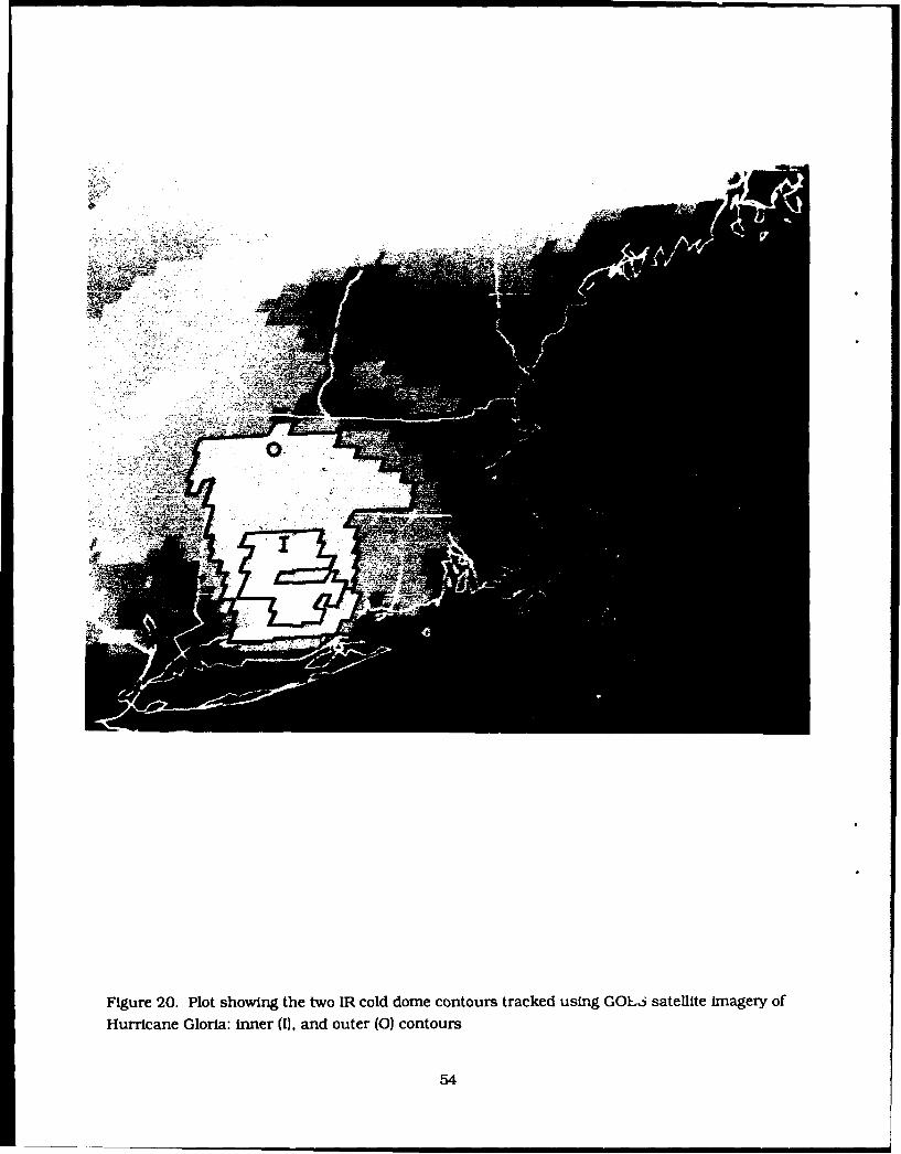
Figure 20. Plot showing the two IR cold dome contours tracked using GOLJ satellite Imagery of

Hurricane Gloria: inner (1), and outer (0) contours

54

forecast 1 (diffx)

40.

30.

20.C_

C2 0.C-

r-0.

U°

-20.

-30.

-40.

-50. p • ,-ICN CO "I L

observation number

Figure 2 la. Plots of actual forecast error for SIMEXP (dash). ADSIMEXP (dash-dot).

SIMMOVAV (long/short dash), KALMAN (solid) routines using differences of X location data of

Figure 19 for one-interval forecasts

55

forecast 2 (diffx)

40.

30.

20.C_

Co.C

0.

2-io. .

-20. -

-30. \

-40.

-50.C'XJ (-r) (flCC:

observation number

Figure 2 1b. Plots of actual forecast error for SIMEXP (dash), ADSIMEXP (dash-dot),

SIMMOVAV (long/short dash), KALMAN (solid) routines using differences of X location data of

Figure 19 for two-interval forecasts

56

forecast 3 (diffx)40.

30.

20.

Cc- 0.C-

r" 0

-20.

-30.

-40.

-50.MU MT 'q-U LO

observation number

Figure 21c. Plots of actual forecast error for SIMEXP (dash). ADSIMEXP (dash-dot).SIMMOVAV (long/short dash), KALMAN (solid) routines using differences of X location data of

Figure 19 for three-interval forecasts

57

forecast I (diffy)

40.

30.

20.C-

cc! 0. XC-

-' -10. '

-20.

-30.

-40.

-50.C%) MD LO

observation number

Figure 22a. Plots of actual forecast error for SIMEXP (dash), ADSIMEXP (dash-dot),SIMMOVAV (long/short dash), KALMAN (solid) routines using differences of Y location data ofFigure 19 for one-interval forecasts

58

forecast 2 (diffy)

40.

30. -

20.C-

210. \C-

-r"10.4 o. -

-20.

--30.

-40.

-50. - ' ' "

observation number

Figure 22b. Plots of actjal forecast error for SIMEXP (dash), ADSIMEXP (dash-dot).

SIMMOVAV (long/short dash), KALMAN (solid) routines using differences of Y location data of

Figure 19 for two-interval forecasts

59

forecast 3 (diffy)

40.

30.

20.010.C-CD

u -.-20.\

-30.

-40.

-50.CxU M 1: L) CL

observation number

Figure 22c. Plots of actual forecast error for SIMEXP (dash), ADSIMEXP (dash-dot).

SIMMOVAV (long/short dash), KALMAN (solid) routines using differences of Y location data of

Figure 19 for three-interval forecasts

60

'": N CM CV)u,) -y l oo iS

co cc

0 £a cy CVza

T- ti CM 7-V

P- C02 a*

00 C0 c 02C-ce) .q a; a;

4)~ 29 EgG - r- r-

,...T - LO ) mt C.) C=9L U" COt £

E .4 14) Li

V - r- cm CV) CC) -C'o £2 C.L

.z Qi; £0;C

0r) CD 0 C1 cm to

cm D 0 0 C14 £o

LO CV) lw in a; ,'g .: r- cc r-

0D L O go P-

-cc C') C'

r- to. :=I, £

. £0u£0 £

zz toC-1z~

- = C.)-i(AC1 toJ co £0 -

£0 cc-zo-0 C.. )A

CC 0to Li- to CC)

.ocOU CO Ln LUF F - £0

cc 4c £0 Cr') to cv) x , C4LA Lo-0UaCO C') £0COD

cro co m CD £O) CO

C.)U ~ ' n 0 t

LU £D m) t) £0a* C

L- LOt C M r

uO 0 04 CO) £o to £o to

CL U-) CL Cci £0 C- cc; c adFzL'X-e in to to m0 4m

,a,.O.LU

C'I-

F-

61

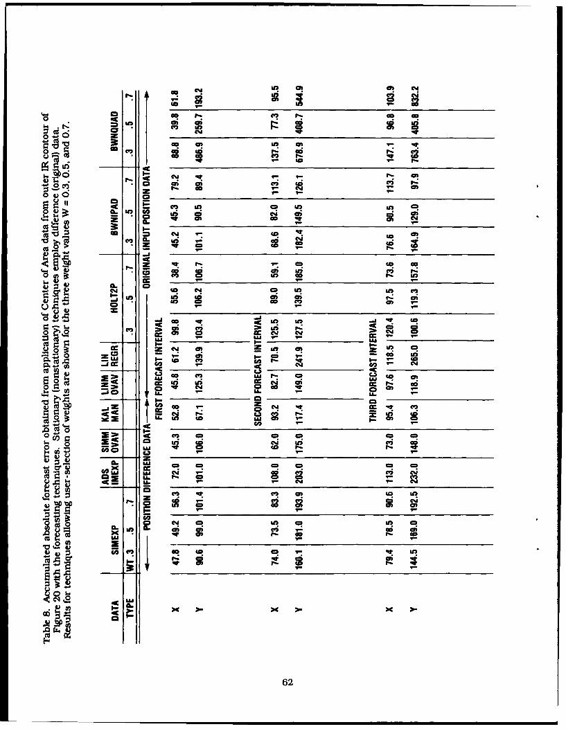
w aa c cm

Go C4

40 T- T0 - 2OD P.r-

tov 3: co 1r

a a!4)oY 1

o ris a; M- cc COD

(C 2 i- a 2L

4 9

F.- C., OR

. a X0 co a) U7 4 P

c 'in ra;

-1 P.2 co COD a)u Q .

-JPZQ0 40 cc;440!z U C O

co) 40 cc CV) -

-~V II. 4

v .3 a* N0 U P- C ao. AU 10 C

mc c C% a r: Ccc Ln cr

qte mo2C oL ) V

Lu _ _ _ _ _ _ _._ _ _ _ _ _ _ _ __D_ _

0~I je _ELL._ _ __cc_ _ _ _a)_CD

622

forecast I (x)

40.

30.

20.C_

-0.C-

-30.

-40.

-50. I ,

observation number

Figure 23a. Plots of actual forecast error for LINMOVAV (dash), HOLT2P (dash-dot),

BWN1PAD (long/short dash), BWNQUAD (solid) routines using X location data of Figure 19 for

one-interval forecasts

63

forecast 2 (x)

40. -

30.

20.C-

, _ 10.C_CD

-20.

-30.

-40.-50. ' "

-I "qn LO

observat i on number

Figure 23b. Plots of actual forecast error for LINMOVAV (dash), HOLT2P (dash-dot),

BWN IPAD (long/short dash), BWNQUAD (solid) routines using X location data of Figure 19 fortwo-interval forecasts

64

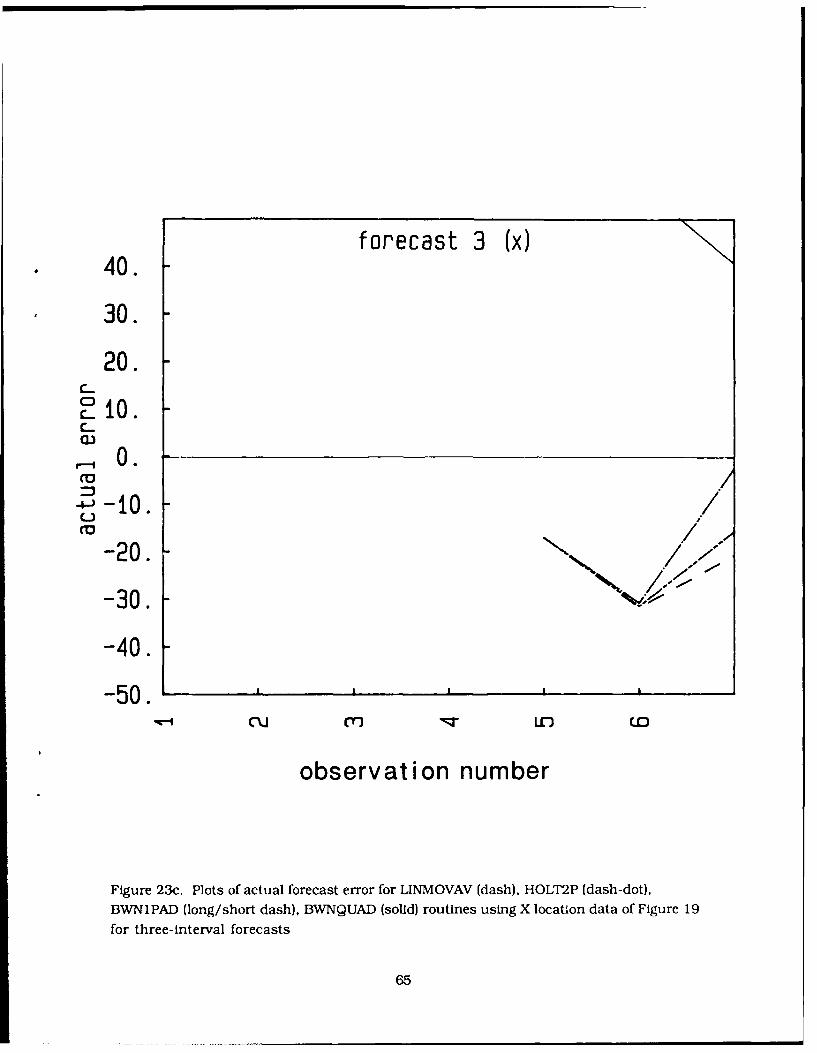
forecast 3 (x)

40.

30.

20.C_

C210.C-

~0.

-10. 7C_,

-20. " .. !

-30. "

-40.

-50.aa

-Ij M "T IO LO

observation number

Figure 23c. Plots of actual forecast error for LINMOVAV (dash), HOLT2P (dash-dot),

BWN1PAD (long/short dash), BWNQUAD (solid) routines using X location data of Figure 19

for three-interval forecasts

65

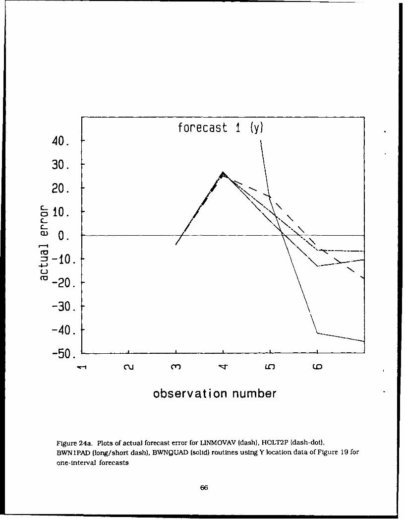
forecast I (y)

40.

30.

20. -

i0. /C-.

-0.

obs r a~4-)UN

~-20.

-30.

-40.-50.II

observat ion number

Figure 24a. Plots of actual forecast error for LINMOVAV (dash), HOLT2P (dash-dot),

BWN1PAD (long/short dash), BWNQUAD (solid) routines using Y location data of Figure 19 for

one-interval forecasts

66

forecast 2 (y)

40.

30.

20.

CC310.._ \

rO.C_

-,- -10.\ ".x-20.

-30.

-40.

-50.

.

COj Mr n riO

observation number

Figure 24b. Plots of actual forecast error for LINMOVAV (dash), HOLT2P (dash-dot),

BWN1PAD (long/short dash), BWNQUAD (solia) routines using Y location data of Figure 19 for

two-interval forecasts

67

forecast 3 (y)

40.

30. -

20.C_V__ 10. \,\C-

CU

-20.

-30.

-40.

-50. , I

CU C' ) ; LO L

observation number

Figure 24c. Plots of actual forecast error for LINMOVAV (dash), HOLT2P (dash-dot),

BWN1PAD (long/short dash), BWNQUAD (solid) routines using Y location data of Figure 19 for

three-interval forecasts

68

forecast 1/2/3 (x)

40.

30.

20.C_

cc!10.C-

3-( 0 N / _. N

-J-10. N-~-K-

-20. -

-30.

-40.

-50.'''''50 U- O I

observat i on number

Figure 25a. Plot of forecast error for LINREG method using the position data of Figure 19 for one

(dash), two (dash-dot), and three-interval (solid) forecasts: X position data

69

forecast 1/2/3 (y)

40.

30. -

20. /_c_10. /C._w /N, 0. / N

- -10.O0

cca-20.

-30.

-40.

-50.

observation number

Figure 25b. Plot of forecast error for LINREG method using the position data of Figure 19 for one

(dash), two (dash-dot), and three-interval (solid) forecasts: Y position data

70

behaves poorly with use of the outer contour position data (not shown). On one hand the relatively

good performance is somewhat surprising since the LINREG routine weights all data evenly in

deriving the best fit trend line. Observation of the outer contour COA data indicated that these dataexhibit greater nonlinear behavior than for the inner contour data. Thus, the reasons for success are

similar to those previously cited for the KALMAN routine. The LINREG method, by weighting all data

equally, tends to preserve the early trends and is less responsive to trend changes than the other

nonstationary data routines.

Finally, the actual forecast errors obtained from use of radar precipitation band COA movementshown in Figures 26a and b are presented in Figures 27 - 30 and the accumulated absolute errors areshown in Table 9. These COA data are similar to the IR data, except the data series are significantly

shorter and thus emphasize the performance over a short data series. The stationary data routinesbehave in a manner quite similar to that observed with use of IR data. The ADSIMEXP method is

overresponsive and prone to large error, particularly for one-interval forecasts. The KALMAN

method is sluggish in response to sudden change. For one-interval forecasts it incurs the greatest

error of all norstationary routines with use of x position data and minimum error with the y positiondata. The two and three-interval forecast errors are all nearly identical since these forecasts do not

incorporate the sudden change at data number 5 and are simply preserving the early trend in the data.The SIMEXP (weight = 0.3) and SIMMOVAV routines respond similarly. The nonstationary data

routines providing the best performance are the HOLT2P (weight = 0.7) and BWNIPAD (weight = -0.5)

methods. The LINREG method again suffers large error in forecasting one-interval change, again aresult of its inability to preferentially weight new observations over the historical trend.

5.4 Computational Complexity

Such tests displayed some relative strengths and weaknesses of the various techniques andnarrowed the field of potentially useful routines. Additional factors were then considered. First, ease

of implementation is of considerable interest. The computer codes for all the routines have beenconfigured to require a data array transfer between the routine and host program of length no more

than ten 32-bit words. The individual routines themselves vary only from about 10-50 lines of code

for the simplest to most complex methods. Thus computer code length and data storage

considerations are not a useful discriminant.

Another concern is the stability of performance; that is, did routine performance changedrastically with introduction of a new data set? The KALMAN and BWNQUAD routines are examples

where a comp'ete reversal in relative performance was noted. Because the attributes to be tracked andforecast may behave in unpredictable ways, it is highly doubtful that these two routines would beuseful for the broad variation in attribute behavior possible. A related concern is whether the

preferred weighting factors, where user-selection was available, varied with introduction of new data.The preferred weight for the HOLT2P method varied between 0.5 and 0.7, whereas the BWN1PAD

optimum weight remained at a value of 0.5 throughout all tests. Thus the BWNIPAD method is favored

over HOLT2P. since it is not just undesirable, but unacceptable to require determination of an

optimum weight while simultaneously deriving forecasts. The ADSIMEXP method attempts to makesuch an automatic adjustment, however, it continually overreacted to data trend variations. The

SIMMOVAV and LINMOVAV routines appear to offer middle of the road performance, while not

71

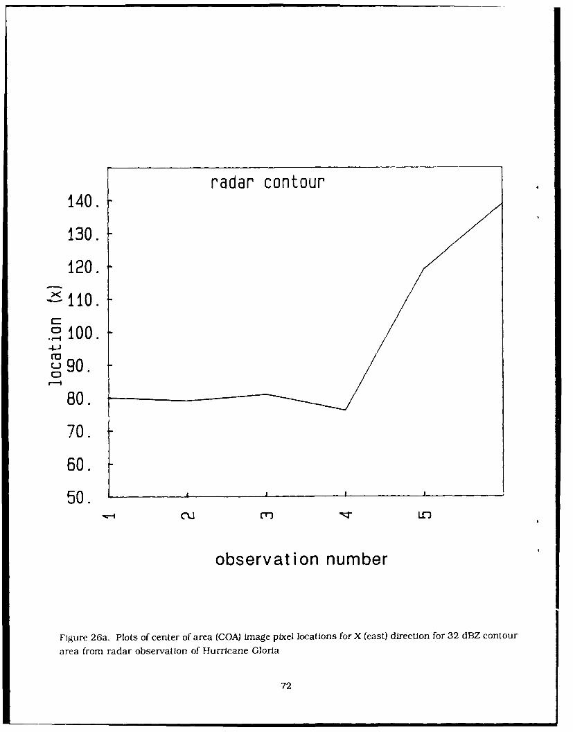
radar contour

140.

130. -

120.

C, 100.

U 90.

80.

70.

60.

50.

observation number

Figure 26a. Plots of center of area (COA) image pixel locations for X (east) direction for 32 dBZ contour

area from radar observation of Hurricane Gloria

72

radar contour170.

160.

150.

- 140.

.I 130. -4 -)

u 120.C3)

110.

100.

90.

80.

observation number

Figure 26b. Plots of center of area (COA) Image pixel loca tlons for Y (north) direction for 32 dBZ

contour area from radar observation of Hurricane Gloria

73

forecast 2 (diffx)

50.

30.C_

E10..1

Ca10. 0

-30.

-50.

-70.°

observation number

Figure 27a. Plots of actual forecast error for SIMEXP (dash). ADSIMEXP (dash-dot). SIMMOVAV(long/short dash), KALMAN (solid) routines using differences of X location data of Figure 26 for one-interval forecasts

74

forecast I (diffx)

50.

30.C_

0.-0.

r-I04-J

- 30.

-50.

-70., ,CU M U-)

observation number

Figure 27b. Plots of actual forecast error for SIMEXP (dash), ADSIMEXP (dash-dot). SIMMOVAV(long/short dash), KALMAN (solid) routines using differences of X location data of Figure 26 for two-interval forecasts

75

forecast 3 (diffx)

50.

30.C-k0.

-10.

-30.

-50.

-70. ,C\jm LO)

observation number

Figure 27c. Plots of actual forecast error for SIMEXP (dash), ADSIMEXP (dash-dot), SIMMOVAV(long/short dash). KALMAN (solid) routines using differences of X location data of Figure 26 forthree-interval forecasts

76

forecast i (diffy)

50.

30.C-

E 0 .

Z3 -10.

-30.

-50.

-70.,

observation number

Figure 28a. Plots of actual forecast error for SIMEXP (dash), ADSIMEXP (dash-dot), SIMMOVAV

(long/short dash). KALMAN (solid) routines using differences of Y location data of Figure 26 for

one-interval forecasts

77

forecast 2 (diffy)

50.

30.C-

-10.

CD ---- -10.-----I

-30.

-50.

-70 . , , p

observation number

Figure 28b. Plots of actual forecast error for SIMEXP (dash), ADSIMEXP (dash-dot), SIMMOVAV(long/short dash), KALMAN (solid) routines using differences of Y location data of Figure 26 fortwo-interval forecasts

78

forecast 3 (diffy)

50.

30.C_C)

Li-o.ID

Z3-10.

CO,

-30.

-50.

-70.CU M ~ --I )

observation number

Figure 28c. Plots of actual forecast error for SIMEXP (dash), ADSIMEXP (dash-dot), SIMMOVAV

(long/short dash), KALMAN (solid) routines using differences of Y location data of Figure 26 for

three-interval forecasts

79

forecast 1 (x)

50.

30.C_

o .

C-10.CO

-30.

-50.

-70 , , ,

observation number

F'gure 29a. Plots of actual forecast error for LINMOVAV (dash), HOLT2P (dash-dot), BWNIPAD

(long/short dash), BWNQUAD (solid) routines using X location data of Figure 26 for one-

interval forecasts

80

forecast 2 (x)

50.

30.4-

cc~

-30.N

-70. \CU

observation number

Figure 29b. Plots of actual forecast error for LINMOVAV (dash), HOLT2P (dash-dot), BWNIPAD(long/short dash), BWNQUAD (solid) routines using X location data of Figure 26 for two-

interval forecasts

81

forecast 3 (x)

50.

30.C-0

10.

cca( 0 .

-50.• -' .... ..

-70.-

observation number

Figure 29c. Plots of actual forecast error for LINMOVAV (dash). HOLT2P (dash-dot), BWN1PAD

(long/short dash). BWNQUAD (solid) routines using X location data of Figure 26 for three-

interval forecasts

82

forecast 1. (y)

50.

30.C-0

CE-10.

Ca

-30.

-50.

-70.C'J M _T )

observation number

Figure 30a. Plots of actual forecast error for UNMOVAV (dash), HOLT2P (dash-dot). EWVNIPAD(long/short dash), BWNQUAD (solid) routines using Y location data of Figure 26 for one-interval forecasts

83

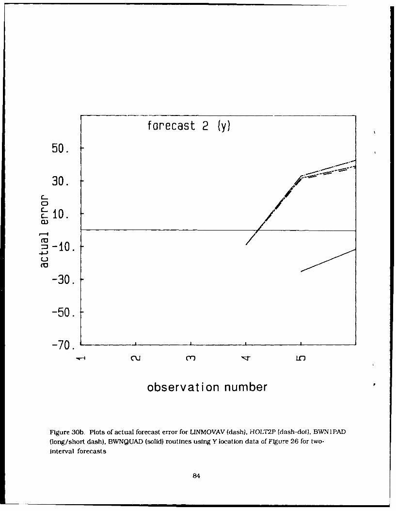
forecast 2 (y)

50.

30. ~/J

CE 10.'I /~-I0.

-30.

-50.

-70. L j

observation number

Figure 30b. Plots of actual forecast error for LINMOVAV (dash), HOUI2P (dash-dot), BWN I PAD(long/short dash), BWNQUAD (solid) routines using Y location data of Figure 26 for two-interval forecasts

84

forecast 3 (y)

50.

30.C-

CE10.

= -10.~4-)

- 30.

-50.

-70.

observation number

Figure 30c. Plots of actual forecast error for LINMOVAV (dash), HOLT2P (dash-dot), BWN1PAD(long/short dash), BWNQUAD (solid) routines using Y location data of Figure 26 for three-interval forecasts

85

00

C3C L2z 1

Vo 3om C)C4 r1 0 0 s.. C-CMC C

zc @0i -9 Cr-

a* CD f-

0c Lq CC! Y C LqCL LO 0 - M c

C# CLC- V- Lei i a; C-

cc Li co p1

CL CN~ CV mCq L

64 LIn c a;fi OLn fr-Z~C U UMa i

o) co r- .V.

0 01 -le - C- r- 1

u~ = C7 0!-c r03 li

0 CC

I CO (0 S Co CCD '

tv 0 1, L n 0 c )

_- C4 a) COjL

CD La S 1 Nq Woa ; 01 = " cm

a: cc (r) CD U2 L La:E qc CO; La COc; ~

L L @0j Cl LO @0Ln

co x- w1L a L

C3 LL U7 cc co ccO

Cu-C

qr C~lcm r86

providing for the flexibility offered in user-selected weighting schemes. The LINREG performed better

than expected, rivaling the BWN1PAD method on numerous occasions. Although it responds slowly to

new data trends it does easily accept non-uniformly spaced data. This last point should not be taken

lightly, for the other routines currently assume uniformly spaced data. Although an aperiodic data

series can be modified to develop a uniform time base, this would require some additional computer

code and calculations.

The efficiency, or speed, of the various routines is also of vital concern. If a large number or

parameters are to be tracked and forecast, then the fastest routine, assuming comparable accuracy,

will best support the real-time operational mode. With the routines under consideration, speed

effectively translates into the number of mathematical operations required to make a simple forecast.

The numbers of operations, utilizing the exact algorithm after reception of an updated data value are

shown m Table 10 for the more reasonable techniques (number of computations to perform data

differencing for stationary routines are included in cited numbers).

The SIMMOVAV and SIMEXP techniques, even employing difference data, are at least twice as

fast as the HOLT2P and BWN1PAD techniques on original data, and at least five times as fast as the

LINREG and KALMAN methods. After taking into consideration all factors the SIMEXP and

BWNIPAD methods were chosen as the primary forecast routines. It is quite likely that a two-tiered

approach, where both routines would be available for use could be employed. This would require

monitoring either the variation (variance, trend, etc.) of the data being received, or the forecasts being

developed, in order for real-time selection to be made. Finally, the LINREG method was also retained

in the event It became necessary to employ aperiodic time series data.

5.5 Reconstruction

The contour segments derived from the forecast attributes must be joined together to form a

continuous and meaningful physical contour. The methods under consideration, as demanded by the

desire to obtain real-time operation, are simple and quick. Only two cases need be considered.namely, when successive segments do not touch and when the segments overlap. In the overlap case,

the simple rule is simply to discard those portions of segments beyond the overlap point which would

not be part of a continuous boundary. For the non-intersecting case, the object is to fit a line segment

between the end points. This can be accomplished by: (1) extending the segments on both sides until an

intersection is obtained, (2) fitting a polynomial across the gap, or (3) fitting a straight line segment

across the gap if the segment would be short and the included angles between the new segment and the

original segments are near 180 degrees.

EL CONCLUSIONS

A methodology has been developed for the short-term forecasting of cloud and precipitation

fields. It employs pattern recognition techniques to extract the useful features from the data field and

extrapolative techniques to project these features into the future. The methodology also relies heavily

on the use of data reduction techniques that significantly reduce the amount of information that must

be tracked and forecast. The methodology is generic in the sense that it may be applied to any data

87

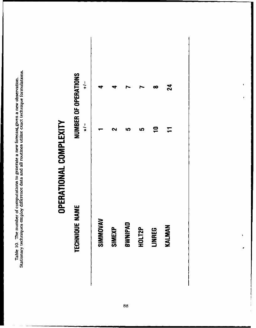
COD0 zP + qt q - r- cc

.0 v LU0 C0

LA.

.?: u LU

~~CD

CI

0.

0~

*cm 2

z

UL

0. 0LUL

a.. "-A cc.

- LU

88

which can be represented as a two-dimensional distribution. For the 0 - 0.5 hr forecast problem

addressed here, the primary data source is radar reflectivity factor. Use of GOES satellite data, having

a temporal scale comparable to the maximum forecast interval, could be employed as an indicator of

the overall large scale environment, but is not incorporated in the quantitative forecasting methods.

The methodology is broken into the four component steps of (1) data preprocessing. (2) feature

definition and extraction, (3) attribute definition and change determination, and (4) attribute

forecasting and feature reconstruction. The techniques employed within each step were strongly

influenced by the desire to develop a real-time capability.

The features tracked are contours of radar reflectivity factor, or equivalently, precipitation

intensity. The contour data, on horizontal grids at selected heights, are composited fields obtained

either by averaging vertical segments or by taking the maximum value above each grid point. The

contour data are smoothed by median and lowpass filters to remove data gaps, errors, and noise.

Initial methods considered for describing whole contours were shown to be inadequate for

accurate measurement of preferential evolution and displacement along the contours. The processes

of feature definition and extraction focuses on two primary algorithms for segmentation of contours.

One method involved objectively segmenting the contour into straight line segments of varying

length. A second method employed fixed length segments, typically 10 - 25 percent of the entire

contour length. The individual segments are describ-d in terms of attributes. a highly limited set of

quantities that accurately describe each segment. Examples of attribute quantities include segment

length, starting location of 'he segment, orientation, and distance from some global reference

location.

The evolution of features was determined by monitoring the changes in the segment attributes

between successive observations and developing a time history of these values. These data form the

data base to be used by the forecasting process.

A number of forecasting techniques were investigated by observing their quantitative andqualitative performance with limited sets of generated and real test data. The generated data included

simple time series representing stationary data with added noise, and noise-free linear and quadratic

trends. The real test data were derived from radar and satellite observations of features associated

with Hurricane Gloria. Tested techniques ranged from simple moving filters to triple smoothing

quadratic filters. It was determined that estimating quadratic trends from data where erratic and

significant changes could occur could easily defeat the quadratic method. Techniques that

automatically determine new weights for current and past observations are found to either overreact

(Adaptive Exponential Smoothing filter) or underreact (Kalman filter) to these sudden changes.

Ultimately two techniques were selected: (1) the Simple Exponential Smoothing filter, and (2) the

Brown One-Parameter Adaptive Smoothing filter. Whereas the exponential filter would operate on a

time series obtained from the differences of the attributes between observations, the Brown filter

operates on the original attribute observations. These routines worked well with stationary and

linear time series data. More complicated trends are handled fairly well by these routines due to their

ability to preferentially weight the most recent observations. From the time series of attribute data,

the forecasting process develops future expectations of attribute values. These values completely

determine future contour segments, and ultimately the future contours.The software developed represents an extensive library of routines. Currently, a major portion

of these routines are accessed from an executive program through interactive menu-driven operations.

89

Further testing of the segment line and curve fitting) routines is required to fine tune thesetechniques. The process of reconstruction of the forecast segments to produce accurate and pleasingfuture contours has not been fully completed. Also, this software package does not currently facilitatereal-time operation, a definite initial objective of the effort. These efforts of fine tuning existingroutines and development of an executive program for real-time operation will be accomplished in anew more comprehensive short-term forecasting program to begin shortly.

90

References

1. Sadoski, PA., Egerton, D., Harris, F.I, and Bohne, A.R. (1988) The Remote Atmospheric ProbingInformation Display (RAPID), AFGL-TR-88-0036, AD A196314.

2. Bohne, A.R and Harris. F. Ian (1985) Short Term Forecasting of Cloud and Precipitation,AFGL-TR-85-0343. AD A169744.

3. Mohr, C.G. and Vaughan, R. (1979) An economical procedure for Cartesian interpolation anddisplay of reflectivity factor data in three-dimensional space, J. AppL MeteoroL 18:661-670.

4. Foote, G.B. and Mohr, C.G. (1979) Results of a randomized hail suppression experiment innortheast Colorado. Part VI: Post hoc stratification by storm intensity and type, J. AppLMeteoroL 18:1589-1600.

5. Harris, F.I. and Petrocchl, P.J. (1984) Automated Cell Detection as a Mesocyclone PrecursorTool, AFGL-TR-84-0266, AD A154952, 32 pp.

6. Pratt, William K (1978) Digital Image Processing, Wiley-Interscience, New York.

7. Rinehart, RLE. (1979) Internal Storm Motions from a Single Non-Doppler Weather Radar,NCAR/TR- 146+STR, National Center for Atmospheric Research, Boulder, CO. 262 pp.

8. Smythe, G.R. and Zrnic', D.S. (1983) Correlation analysis of Doppler radar data and retrieval ofthe horizontal wind, J. Cnim. AppL Meteor. 22:297-311.

9. Smythe, G.R and Harris, F.I. (1984) Sub-Cloud Layer Motions from Radar Data UsingCorrelation Techniques, AFGL-TR-84-0272, AD A156477.

10. Dudani, SA. (1976) Region extraction using boundary following, Pattern Recognition andArtifical Intellence (C.H. Chen, editor), Academic Press, Inc., New York, NY, pp. 216-232.

11. Clodman, S. (1984) Application of automatic pattern methods in very-short-range forecasting,Proc. Nowcastlng II Symposium, Norrkoping, Sweden, ESA SP-208.

12. Williamson, D.L. and Temperton, C. (1981) Normal mode initialization for a multilevel grid-point model, Part I: Nonlinear Aspects, Mon. Wea. Rev. 109:744.

13. Dennis, J.E., Gay, D.M., and Welsch, RE. (1977) An Adaptive Nonlinear Least-SquaresAlgorithm, Cornell Computer Science TR77-32 1.

14. Freeman. H. (1961) On the encoding of arbitrary geometric configurations, IRE Trans. Electron.Corput, EC-10:260-269.

91

References

15. Wu, IU-De (1982) On the chain code of a line, IEEE Trants. Pat. AnaL and Mach. InteL., PAMI-4(#3):347-353.

92

Appendix A

Forecasting Algorithms

Two specific algorithms were selected for use in the RAPID methodology for deriving forecasts of

attribute variables. These were the Simple Exponential Filter and the Brown's One-Parameter LinearExponential Filter. The particular formulations are presented in the following sections.

Al. SIMPLE EXPONENTIAL FILTER

This filter is designed to operate on stationary data. The data is assumed composed of two

components, a population mean and added noise. The form of the filter is

F(t + 1) = WXt) + (1 -W) F(t) (Al)

F(t+ 1) = WXt)+W(I-W)Xt-I)... W (1 -W)**N - 1 Xt - (N - 1)) (A2)

F(t+ 1) = F(t) +W(x M -F(t)) (A3)

in its various forms. Here Fit) is the previous forecast valid for the current time. F(t + 1) is the current

forecast for the next observation period. X(t) is the current observation, and W is a user-selectableweighting factor. The formulation (AI) requires only storage of the current forecast and the weighting

factor while still empoying all data ever input into the filter (A2). As shown in (A2) a small value of W

effectivelV results in near uniform weighting of all data ever input into the filter, whereas a largeweight value biases the filter result towards current observations. In this manner the filter can be

biased to the historical mean (low signal to noise ratio) or can adjust to new trends (high signal to

noise ratio). This adjustment feature Is shown more clearly in (A3) which may be interpreted as a new

93N

forecast being derived from the previous forecast and an adjustment proportional to the errorincurred from the previous forecast.

Because of its simple structure and ease of implementation, this filter may efficiently be usedwith difference data as input, where the input series is now the differences between successive

observations. This allows application where the forecast variable may contain a linear trend. Theresults with test data indicated that preferential weighting should be given to the gistorical triend to

diminish noise effects and overestimation of the rate of change. A value of W = 0.3 was found most

suitable.

A2. BROWN ONE-PARAMETER LINEAR EXPONENTIAL FILTER

This filter is designed for use with data exhibiting an underlying linear trend. It performs anumber of smoothing operations to obtain estimates of the linear equation parameters and filter out

the random noise component. This technique may be written as

F(t m) = A(t) + B(t) m (A4)

where

A(t) = Si(t) + (Si(t) -S2(t)) (A5)

B(t) = (Sl(t) -S2(t))W/(I-W) (A6)

Sl(t) = WX(t)+(I-W Si(t-I) (A7)

S2(t) = W Slt) + (1 -W) S2(t - 1) (A8)

where F(t + m) is the forecast for m intervals from the current (t) time, X(t) is the current observation,

W is a user-selected weight, and A(t), B(t) are the automatically adjusting parameters of the linear trendequation. Setting W large encourages the filter to preferentially adjust the coefficients of the linearequation to the new observations rather than the historical data. This effectively makes the

assumption that noise is a minor contribution and that trend changes suggested by new observationsshould be heavily weighted. If the signal to noise ratio is expected to be large and heavy smoothing isrequired to bring out the trend then a smaller weight must be applied. The test data suggested that a

value of W = 0.5 would accommodate a wide range of data types and is the value employed in RAPID.

*U.S. GOVERNMENT PRINTING 0FFICE:1989-600-0 00 01l

94