AD-A258 904

AFIT/GAE/ENY/92D-17

HELICOPTER FLIGHT CONTROL SYSTEM DESIGNUSING THE LINEAR QUADRATIC REGULATORFOR ROBUST EIGENSTRUCTURE ASSIGNMENT

THESIS

Dempsey D. Solomon, CPT, USA D T Ic

C_7 AFI T/GAE/ENY/92D- 17 F ft

A~jtio 719933

Approved for public release; distribution unlimited

(0

93 1 04110

DISCLAIfI' NOTICE

THIS DOCUMENT IS BESTQUALITY AVAILABLE. THE COPY

FURNISHED TO DTIC CONTAINED

A SIGNIFICANT NUMBER OFPAGES WHICH DO NOTREPRODUCE LEGIBLY,

AFIT/GAE/ENY/92D-17

HELICOPTER FLIGHT CONTROL SYSTEM DESIGN USING THE LINEAR

QUADRATIC REGULATOR FOR ROBUST EIGENSTRUCTURE ASSIGNMENT

THESIS

Presented to the Faculty of the School of Engineering

of the Air Force Institute of Technology

Air University

In Partial Fulfillment of the

Requirements for the Degree of

Master of Science

by

Dempsey D. Solomon, B.S.

Captain, USA

December 1992

Approved for public release; distribution unlimited

Acknowl edaements

My thanks to the staff and faculty at AFIT, especially

Dr. Bradley S. Liebst, who provided an outstanding environment

in which to learn as well as their knowledge and guidance.

Also, thanks to Mr. Doug Burkholder who allowed me to learn as

little about computers as possible.

I would especially like to thank Cindy, Matthew and A.J.

who teach me a little more every day.

Dempsey D. Solomon

Aoaoesion ForNTIS GRA&I &rDTIC TABUnannounoCe 0JustLfIcation

Dl;T •~ "-> ..... _ __ __ _

S........ : utli,/D____

TABLE OF CONTENTS

Page

Acknowledgements ............ ................... ... ii

List of Figures ................. .................... v

List of Tables .............. .................... .. vi

List of Symbols ............. .................... .. vii

Abstract .................... ....................... x

I. Introduction ....................... 1

Helicopters ............... ......... . ._1Flight Control Systems Design ..... ....... 6Program Background .......... ............. 8

II. Cross Coupling Extension ..... ............. ... 11

Theory ............ ................... ... 11

General .. ............ .......... ... 11Cross-Coupling . . . ...... .......... ... 12Matrix Definiteness ... .......... ... 14

Algorithm Changes ......... ........... .... 16

Using the Standard Regulator .... ...... 17Creating Q, R and S .... .......... ... 18Eigenvalue Pairing .... ........... ... 20

III. Stability Robustness ...... .............. ... 24

Theory ................................... .. 24Achievable Robustness with Cross Coupling

Weights ........ ................ ... 25

V. Results ............... ...................... .. 33

Inputs ................ .............. ... 33Analysis of Results. ..... ............. ... 38AH-64 Results ......... ............... ... 40

Achieving a Closer Solution .... ...... 40Convergence Tolerance Effects on

Stability Margins ... ......... ... 44

iii

UH-60 Results ......... ................ ... 47

Dimensional Effects. ....... . ... 47Elgenstructure Input Order Effect . 49Weighting Element Changes .. ....... .. 50

V. Conclusions ............. .................... ... 53

VI. Recommendations .......... ................. ... 54

Appendix A: AH-64 Model ........ ............... ... 56

Appendix B: UH-60 Mathematical Model ... ......... ... 58

Appendix C: Source Code ........ ............... ... 59

Appendix D: Operating Instructions .... .......... ... 77

Bibliography .............. ..................... ... 83

Vita .................. ......................... ... 86

iv

List of Fioures

Figure Page

1 Example of Eigenvalue Pairing 22

2 AH-64 Eigenvalue Pairing 35

3 AH-64 Minimum Singular Values 40

V

List of Tables

Table Page

I Desired Closed Loop Eigenstructure 33

II Sample 3 Convergence 37

III Summary of AH-64 Results (Unity Weighting) 39

IV AH-64 Achieved Closed Loop Eigenstructure(Run 3) 41

V AH-64 Achieved Closed Loop Eigenstructure(Run 6) 42

VI Summary of UH-60 Results (Unity Weighting) 46

VII UH-60 Achieved Eigenstructure 51

vi

List of Symbols

a minimum singular value of return difference matrix

6. lateral cyclic control movement

6b longitudinal cyclic control movement

6. collective control movement

6P tail rotor control movement

a pitch angle

6, ih eigenvector difference minimization parameter

eigenvalue

X. achievable eigenvalue

desired eigenvalue

redefined control vector

p arbitrary constant

0 roll angle

o minimum degree of stability

9 minimum singular value

0 frequency

infinity

o degrees

* multiplication

if integral

I summation

A state matrix

Ago non-dimensional state matrix

ACLS closed loop state matrix

ANEW redefined state matrix

vii

B control matrix

6 non-dimensional control matrix

det determinant of a matrix

dt differential element of time

Ed diagonal matrix of desired eigenvalues

e base of natural logarithms

Fe eigenvalue weighting matrix

Fv eigenvector weighting matrix

G redefined regulator gain matrix

I identity matrix

IGM independent gain margin

IPM independent phase margin

i or j square root of negative one

J LQR performance index

3 algorithm performance index

JA eigenvalue contribution to )

K feedback gain matrix

kmax maximum optimization iterations

MHN matrix used to create weighting matrix QRS

n number of states

P Riccati equation solution matrix

p roll rate

q pitch rate

Q LQR state weighting matrix

j or QRS positive definite weighting matrix formed by Q, R

and S

viii

QH matrix used to create state weighting matrix Q

QNEW redefined state weighting matrix

r yaw rate

R LQR control weighting matrix

RN matrix used to create control weighting matrix R

r-code code specifying type of R matrix to be used

S LQR cross coupling weighting matrix

s-code code specifying type of S matrix to be used

SN matrix used to create weighting matrices

tol convergence tolerance for algorithm

u control vector

u longitudinal velocity

v lateral velocity

v. achieved eigenvector

vd desired eigenvector

Vd matrix of desired eigenvectors

w vertical velocity

x state vector

A derivative of state vector

XGUESS vector used to minimize performance index

z, it' element of vector z

ZIJ element in it" row and jt' column of matrix Z

ZT transpose of matrix Z

Z-1 inverse of matrix Z

Ze Hermitian transpose of matrix Z

ix

AFIT/GAE/ENY/92D-17

Abstract

This thesis applies modern, multi-variable control design

techniques, via a FORTRAN computer algorithm, to U.S. Army

helicopter models in hovering flight conditions.

Eigenstructure assignment and Linear Quadratic Regulator

(LQR) theory are utilized in an attempt to achieve enhanced

closed loop performance and stability characteristics with

full state feedback. The addition of cross coupling weights

to the standard LQR performance index is specifically

addressed. A desired eigenstructure is chosen with a goal

of reduced pilot workload via performance characteristics

and modal decoupling consistent with current helicopter

handling qualities requirements. Cross coupling weighting

is shown to provide greater flexibility in achieving a

desired closed loop eigenstructure. Also, while the

addition of cross coupling weighting is shown to eliminate

stability margin guarantees associated with LQR methods, the

study shows that the modified algorithm can achieve a closer

match to a desired eigenstructure than previous versions of

the program while maintaining acceptable stability

characteristics.

x

HELICOPTER FLIGHT CONTROL SYSTEM DESIGN USING THE LINEAR

QUADRATIC REGULATOR FOR ROBUST EIGENSTRUCTURE ASSIGNMENT

j. Introduction

This thesis applies modern, multi-variable control

design techniques, via a FORTRAN computer algorithm, to U.S.

Army helicopter models in hovering flight conditions.

Eigenstructure assignment and Linear Quadratic Regulator

(LQR) theory are utilized in an attempt to achieve enhanced

closed loop performance and stability characteristics with

full state feedback. The addition of cross coupling weights

to the standard LQR performance index is specifically

addressed. A desired eigenstructure is chosen with a goal

of reduced pilot workload via performance characteristics

and modal decoupling consistent with current helicopter

handling qualities requirements. This work builds upon

previous efforts by Robinson [1] and Huckabone [21 at the

Air Force Institute of Technology (AFIT), the major

difference being the addition of cross-coupling weighting in

the LQR performance index.

Helicopters

Helicopters serve as a good platform for the

application of automatic control. The aerodynamic and

structural design of rotary winged aircraft create inherent

problems with regard to stability and control. In order to

1

apply the tools of control design, a mathematical model of

the system is needed. McRuer [3:chap 4] presents the

assumptions and techniques used to represent an aircraft as

a set of linear differential equations with constant

coefficients, or equations of motion. Reid [4:chap 6]

provides the techniques by which these equations can be

represented as transfer functions or via the state space

model

z = A +÷J (1)

The state space model is used for the design technique

presented in this thesis.

Two helicopter models are used in this thesis. One is

based on the AH-64 (Apache) attack helicopter [5] the other

is the UH-60 (Blackhawk) utility helicopter [6]. Both

aircraft are considered to be conventional helicopters in

that they have a single main rotor to produce primary lift

and a single tail rotor to produce anti-torque and

directional control forces. The models used here represent

the aircraft in hovering flight.

The state vector x in equation (1) is the column vector

comprised of the following respective states:

u - longitudinal (long) velocity (vel) [feet/second]

v - lateral (lat) velocity [feet/second]

w - vertical velocity [feet/second]

2

p - roll rate (radians/second]

q - pitch rate [radians/second]

r - yaw rate [radians/second]

0 - roll angle [radians]

o - pitch angle [radians]

The input vector u is the column vector comprised of the

following respective inputs:

.- collective

.- longitudinal cyclic

6, - lateral cyclic

6, - tail rotor

Collective input refers to a simultaneous change in the

angle of attack of all the main rotor blades that causes a

change in magnitude of the lift produced by the main rotor.

Cyclic input refers to independent angle of attack changes

of the blades that result in a change of main rotor lift

direction. Tail rotor input is similar to collective input

applied to the tail rotor. For the AH-64 model, the inputs

are expressed in degrees of blade movement, while the UH-60

inputs are expressed as inches of control movement.

Standard sign conventions for states and controls are used

as presented in reference [3].

The A and B matrices of equation (1) contain the

constants of the equations of motion. These matrices are

3

presented in appendices A and B for the AH-64 and UH-60,

respectively. The AH-64 model has been non-dimensionalized

as described by Huckabone [2:52-54].

The purpose of designing an automatic control system

for an aircraft is to enhance its handling or flying

qualities.

Flying qualities determine the ease and accuracywith which a pilot can accomplish the varioustasks or maneuvers that constitute the aircraft'smission. The elements which directly affectflying qualities are the stability and controlcharacteristics of the aircraft which link thecontrollers that the pilot manipulates to theaircraft response states that the pilot desires tocontrol [7:2-1].

Factors that can cause adverse flying qualities are:

instabilities, sluggish response and uncommanded responses.

Specific flying quality requirements for helicopters are set

forth in Aeronautical Design Standard-33 (ADS-33) (8].

Analysis of the open loop eigenstructure of the helicopter

model will reveal the presence of instabilities and state to

state coupling. The B matrix of the helicopter model shows

the control-state coupling that is specifically addressed in

this thesis.

The need to improve handling qualities arises from the

desire to reduce the pilot's workload as much as possible.

This is done to allow the pilot to perform tasks, other than

flying, in conjunction with the aircraft's mission.

Examples of tasks include navigation, communication and

weapon delivery. One way that flying qualities may be

improved is by the reduction of control-state coupling or

4

cross coupling. Ideally, a helicopter pilot should have the

ability to command precise control of the hovering

aircraft's position via direct, single axis control. The

desired control-state coupling is:

Collective - Vertical Velocity

Longitudinal Cyclic - Longitudinal Velocity

Lateral Cyclic - Lateral Velocity

Tail Rotor - Yaw Rate

Automatic Flight Control Systems (AFCS) are currently

utilized in helicopters to reduce pilot workload. One of

the most modern aircraft designs, the MH-60K, employs the

following features to augment flying qualities in a hover:

1. Pitch, roll and yaw stability

2. Cyclic, collective and directional trim

3. Pitch and roll attitude hold

4. Heading hold

5. Altitude hold

6. Coupled hover (inputs through automaticpilot) [9]

These functions greatly enhance the mission effectiveness of

the aircraft and crew in a combat aircraft employing many

complicated weapons systems.

5

Flaht Control Systems Desian

AFCS for helicopters are primarily designed using

classical or single input, single output (SISO) methods.

These methods require that the multiple input, multiple

output (MIMO) state space model of the system be broken down

into scalar subsystems or transfer functions. Even recent

research by Osder and Caldwell concludes that "A practical

process for designing such multiple input, multiple output

helicopter systems starts by decoupling controls into four

single input, single output axes ... [10]." The

simplification of the MIMO system is deemed necessary

because SISO techniques become very complicated when all

input-output relationships are addressed, especially cross

coupling of controls and states. This normally leads

control system designers to limit their focus to the worst

cross coupling areas while ignoring the rest.

As an example, the UH-60 helicopter flight control

system incorporates a mechanical mixing unit designed to

eliminate coupled control inputs [11]. The mixing unit

links only four out of the twelve possible cross couplings

of the desired control-state matches. This is done even

though coupling is present in all of the control-state

pairings.

Modern design techniques allow for direct use of the

MIMO state space model in control system design algorithms.

There is no need to break down an integral model into SISO

subsystems. Thus all the control state relationships,

6

including cross couplings, are considered in the design

process. Two popular MIMO design techniques are

eigenstructure assignment and the Linear Quadratic

Regulator.

Eigenstructure assignment allows control system

designers to prescribe desired closed loop eigenvalues and

eigenvectors for a given system, thus achieving desired

performance characteristics. Garrard and Liebst used

eigenstructure assignment "to design a feedback system for

use in precise hovering control for a modern attack

helicopter. Eigenvalue placement is used for stability

enhancement and eigenvector shaping is used for modal

decoupling [12]." But, as Moore has shown, eigenstructure

assignment does not provide a unique control system design

[13]. This flexibility allows the designer to augment

eigenstructure assignment with additional design methods.

The Linear Quadratic Regulator (LQR) is an optimal

control design method that yields a full state feedback

controller which minimizes the quadratic performance index

Jaf (zPg + uaR/u)dt (2)

0

where Q is the symmetric, positive semi-definite state

weighting matrix and R is the symmetric, positive definite

control weighting matrix. Note that this performance index

is quadratic in both state and control variations from

7

nominal conditions, hence minimizing attempts to maintain

small plant deviations with small control inputs. The LQR

method can provide a robust closed loop solution with

guaranteed stability margins [14:sect 6].

Using the eigenstructure assignment method, the control

system designer can specify the desired performance of a

given system. The LQR method provides a robust design

solution. Combined use of these methods yields the best of

both worlds.

Proaram Backaround

Captain Jeffrey D. Robinson developed an algorithm at

AFIT which utilized eigenstructure assignment and the LQR

method in defining linear, full state feedback gain for

aerospace systems [1]. Robinson's algorithm was written

exclusively for use with the MathWorks Inc. software package

MATLABT" [15] and was limited to eigenvalue assignment

only. Captain Thomas C. Huckabone, also at AFIT, augmented

Robinson's work by introducing eigenvector assignment [2].

Huckabone rewrote Robinson's program in FORTRAN using

MATLABT" only as a method of manipulating input and output.

In addition to newly written routines, Huckabone's work

utilized existing subroutines from the LQGLIB [161 and IMSL

[17] packages available on the AFIT computer system.

8

The algorithm minimizes the performance index

n 3[Fe1 (Ad 2. Vd~ 41Va .t (Vd'i4t)]

where

n = number of states

Fe = eigenvalue weighting matrix

Id = desired closed loop eigenvalue

1. = achieved closed loop eigenvalue

Vd = desired closed loop eigenvector

v. = achieved closed loop eigenvector

Fv = eigenvector weighting matrix

0 = eigenvector minimization constant

The feedback controller is obtained via LQR methods, which

minimize the LQR performance index presented in equation

(2). Specifically, the algorithm varies the LQR performance

index state and control weighting matrices, Q and R

respectively, using an optimization method based upon the

Nelder-Mead simplex algorithm presented in reference [18].

This thesis is a direct extension of Huckabone's work.

His algorithm is modified so that the cross coupling

weighting matrix S is included in the LQR performance index.

9

The performance index is now written as

Jdf (4)

0

The modification was added to provide increased flexibility

in achieving the desired eigenstructure. The algorithm is

then applied to mathematical models of conventional, modern

helicopters in hovering flight conditions. The

eigenstructure and stability characteristics achieved via

the modified algorithm are compared with results that do not

utilize the cross coupling weighting matrix.

10

Ii. Cross Couplina Extension

Theory

The majority of the mathematical theory and equations

necessary for development of the algorithm are reported in

detail by Huckabone [2:9-22]. In particular, Garrard,

Liebst [121 and Moore [13] provide eigenstructure assignment

theory while Ridgely [14] provides LQR theory. Some general

equations are presented below for convenience. The theory

necessary to introduce the cross-coupling weighting matrix S

is presented here in detail.

General. Again, the standard state equation of a

multivariable, linear, time invariant, feedback system is

z = az + Bu (5)

Assuming full state feedback and a B matrix with full column

rank yields a linear, feedback control law of

U = -,Jor (6)

Again, the standard LQR method involves minimizing the cost

function

J=f (z'Q+ a PAWu)dt (7)

0

11

where Q is the symmetric, positive semi-definite state

weighting matrix and R is the symmetric, positive definite

control weighting matrix. From LQR theory, an optimal

feedback gain matrix

- R'3"P (8)

is obtained where the symmetric matrix P is the stabilizing

solution to the algebraic Ricatti equation

PA + AtP+ 9 -P=it'PffP -0 (9)

Cross-Couplina. Introduction of the performance index

Tt (10)

0

allows for weighting and, consequently, minimization of

combined state and control terms (i.e. x,u,) via the

matrix S. The original LQR performance index in equation (7)

allows minimization of pure state and control terms (x,x, or

uuj) only'. The integrand of equation (10) can be expanded

via matrix multiplication to

ZVO+ + + uRV#'z+ +(11)

'The standard LQR performance index is equivalent to the newperformance index when all elements of the matrix S are zero,hereafter referred to as S=[0].

12

Simplifying equation (11) via scalar addition and

substituting back into equation (10) yields the rewritten

performance index

,T7 (z"a + 2xz' + a fJau) dt (12)

0

Anderson and Moore [19:56] show that standard LQR methods

can be utilized to find an optimal feedback solution that

minimizes a performance index written in the form of

equation (12) with the following constraints'

A> 0 (13)

O-1'V k 0 (14)

This is shown by rewriting the integrand of equation (12) as

xz(O5Z-'U') Z+ lPW (15)

where

U u +5'18Z (16)

Via substitution, the original state equation (5) is

*The expressions > 0 and k 0, when used with matrices,refer to the matrix being positive definite and positive semi-definite, respectively.

13

rewritten as

=(A -BR -'O) + B (17)

The redefined LQR problem yields an optimal control law of

P = -'BffmX (18)

where P is now the stabilizing solution to the algebraic

Ricatti equation

P(A-B=Off) +(Ar-BR Bf' P-JPz-1Bzp+(Q-82-'Of) = 0 (19)

The optimal control law for the original system is then

found by combining equations (16) and (18) which results in

u = ---R(Bf + or)z (20)

Matrix Definiteness. In order to apply the cross

coupling theory, the algorithm must utilize a method that

provides a standard LQR problem solver with inputs that

satisfy the constraints of equations (13) and (14). This is

done by creating the positive definite matrix

which satisfies the following necessary and sufficient

14

condition for a positive definite matrix (20:331]

zUDX > 0 for a1 vectors z 0 0 (22)

Defining

S-[(23)

and substituting the partitioned matrix of equation (21)

into the inequality (22) yields

A7rL+ 24ý%% + 4r. > 0 (24)

Setting x1=O yields

ffr• > 0 (25)

when x,*O , which meets the necessary and sufficient

condition for positive definiteness of matrix R, thus

ensuring the constraint of equation (13) is met. Rewriting

the inequality (24) as

Jq( M-I'g9,% + xft > 0 (26)

where

X - X2 + ÷ ='opkx (27)

15

and setting X=O, x,*O yields

z4~(Q-A5RLUV)z1i> 0 (28)

which meets the necessary and sufficient condition for

positive definiteness of matrix [Q-SR-IST ], thus satisfying

the constraint of equation (14). A more general proof for

satisfying these constraints is provided in Kreindler and

Jameson [21:147].

Alaorithm Chances

The original FORTRAN program EIGSPACE, as written by

Huckabone, was changed where necessary to allow the use of

the cross coupling weighting matrix S as described in the

theory presented above. In addition, the program was

cleaned up to eliminate unnecessary procedures. Details

presented in this thesis represent only the major changes

made for this thesis. The original EIGSPACE program and

subroutine descriptions are presented in detail as

appendices A and B of Huckabone's work [2:72-1031. The

LQGLIB package of subroutines and the IMSL subroutine were

not altered and are described in references [16] and [17],

respectively. The modified program is presented in

appendix C. Operating instructions and options are

presented in appendix D.

The major changes to the original algorithm occur in

two subroutines. Subroutine PP is modified to allow use of

a standard LQR solver, in this case the LQGLIB

16

subroutine REG. Subroutine MAKEQRS forms the weighting

matrices Q, R and S. Also, the SORT subroutine was

eliminated as it was unnecessary. Otherwise, the

optimization methods and program flow for the algorithm are

unchanged from that presented in detail in Huckabone's

thesis [2:23-301.

Usina the Standard Reaulator (Subroutine PP). As

stated in the cross coupling theory above, to modify a

standard LQR solver to include the cross coupling weighting

matrix S, the Q and A input matrices are redefined as

a= [I 1Og-IsV (29)

and

hý (A-3R1 5'] , (30)

respectively. The regulator gain matrix of the redefined

problem is then given as

a- -1B p (31)

where P is the stabilizing solution to the Ricatti equation

(19). The optimal control law for the desired problem is

given in equation (20) and yields a regulator gain matrix

for the desired system of

S- (B rip + a V(32)

17

Thus the desired closed loop A matrix for the original

system is

A=AW [A-M2 (33)

Creatina 0. R and S (Subroutine MAKEORS). The

parameters varied by the optimization subroutines are

contained in the vector XGUESS. XGUESS makes up the upper

triangular elements of the matrices QH and RM in the case

where S is not varied. In the case where S is varied,

XGUESS also contains all elements of the matrix SN. In both

cases, the initial XGUESS is set such that Q and R are

appropriately dimensioned identity matrices and, when

appropriate, S=[O1.

In the nonvariable S case, Q and R are formed as in the

MAKEQR subroutine from the original program [2:100] with

S=[O] introduced as input to the PP subroutine. The

following description of how the algorithm creates the Q, R

and S matrices applies only to the non-zero S case. While

setting SN equal to an all zero matrix would properly form

the Q and R matrices in the nonvariable S case, the

algorithm requires that the two cases be handled

differently. Specifically, in the non-variable S case, the

XGUESS vector does not contain the additional parameters for

SN as they would be unnecessarily iterated during the

optimization process.

i8

As stated in the matrix definiteness theory, in order

to allow a variable S in the algorithm, the positive

definite matrix

must be created. This matrix, renamed QRS in the program,

can be formed as

w- , m(35)

where MHN is the real symmetric matrix

(36)

Note that equation (35) is equivalent to

l= r(37)

where * denotes the Hermitian transpose of a matrix.

Ridgely and Banda [14:2-71 provides that as long as MMH is

nonsingular, the eigenvalues of QRS are all positive, hence

QRS is positive definite [20:331]. The initial setting of

MHN and the subsequent iteration process, virtually assure

that MHN will always be nonsingular; however, the algorithm

is designed to yield an error message if this occurs.

19

Substituting the partitioned HM matrix of equation

(36) into equation (35) yields:

S= ......... .... .f + (38 )AW*ff+JWSAWVt I MirV*Mfr + I•~

Thus, the weighting matrices generated by the algorithm are:

= - + muom + iN' (39)

Z - J*lEJ + if.sir (40)

a M WOW + ilnuJ (41)

Eiaenvalue Pairina (Subroutine SORT). As stated

previously, the algorithm minimizes the performance index

n.[Fe lAd '-a )a+lv (vd,,l-OtV.,) FVL(Vd1 -- Ve v,)] (42)

where

n = number of states

Fe = eigenvalue weighting matrix

1d = desired closed loop eigenvalue

1. = achieved closed loop eigenvalue

Vd = desired closed loop eigenvector

v. = achieved closed loop eigenvector

Fv = eigenvector weighting matrix

0 = eigenvector minimization constant

20

The above performance index may not accurately reflect the

designer's desired value during execution of the program.

This is due to the fact that the algorithm must select which

desired and achieved eigenvalues are to be paired together.

(Note that the eigenvectors are paired in accordance with

their respective eigenvalues.) Proper pairing can not be

guaranteed by the program as it has no provisions for

identifying eigenvalues by mode. Currently, the algorithm

pairs the eigenvalues by comparing each achieved value with

the value that is designated as the first desired eigenvalue

and selecting the closest as its complement. This procedure

continues for each desired eigenvalue, according to a

selected order. The original EIGSPACE program attempted to

utilize the SORT subroutine as a method of selecting the

order. The subroutine sorted the eigenvalues in order of

increasing magnitude and was used to sort both the desired

and achieved eigenvalues.

Sorting the achieved eigenvalues was determined to be

unnecessary since the algorithm ignores the sorted order

when determining the closest match. Sorting the desired

eigenvalues was also deemed unnecessary as the user may

select the order when the desired eigenstructure is input to

the program. It is important to note that the input order

is important since different orders can yield different

solutions. A simplified example illustrates this problem.

Figure 1 shows a possible mapping of achieved and

desired eigenvalues. It appears obvious that in determining

21

how close the achieved values are to the desired structure,

a designer would pair the complex achieved eigenvalues with

the complex desired eigenvalues and the real achieved value

with the real desired value. However, if the real desired

value is considered first in the pairing method used by the

algorithm, it will pair off with one of the complex values,

as they are closer. Thus the performance index will not

accurately reflect what the designer would like to define as

closeness. This will affect the minimizing path that the

algorithm takes in searching for the best solution.

2i

0.5

0.5

-OS

-0.5-

-1.5+ - ld

-÷-

-4 -3.5 -3 -2.5 -2 -1.5 -1

rod

Figure 1Example of Elgenvalue Pairing

22

It should also be noted that the input order of the

sign of the imaginary component of desired complex

eigenvalues is important as different pairings may occur for

different orders. The algorithm is written so that the

achieved eigenstructure determined by the DLQGLIB subroutine

EIGVV always yields any complex pairs with the positive

imaginary eigenvalue first. Knowing this, the user can

input the desired eigenstructure accordingly.

For the simplified example above, the input order of

the desired structure to avoid the mismatching problem is

obvious. Unfortunately, higher state problems do not always

provide the same easy insight and the number of permutations

increases dramatically. Thus, the input order of the

desired eigenstructure becomes another designer chosen

parameter.

23

III. Stability Robustness

Theory

Ridgely and Banda [141 present theory for stability

robustness of MIMO systems as well as guaranteed stability

margins using the LQR solution. Specifically, the notion of

independent gain and phase margins is introduced as follows:

Independent gain margins (IGM) are limits withinwhich the gains of all feedback loops may varyindependently at the same time withoutdestabilizing the system, while the phase anglesremain at their nominal values. Independent phasemargins (IPM) are limits within which the phaseangles of all loops may vary independently at thesame time without destabilizing the system, whilegains remain at their nominal values [14:3-73].

The following relationships are shown to exist

1 2.1 (43)T+6 1-l

and

where a is the minimum singular value, for all frequencies,

of the return difference matrix given by

a M infA [xz(Jx-A) --D] (45)

Note that equation (45) must satisfy the constraint a S 1.

24

The inequalities (43) and (44) are conservative, thus they

yield guaranteed minimum stability margins.

Ridgely and Banda [14:sect 71 also derive the Kalman

inequality from LQR relationships, which is:

[Z+R1 X(joZ_-A) .3Ij]T[z+lz(jwZ-A) _IJ3-3 ]Z (46)

Guaranteed LQR stability margins are derived from equation

(46) under the restriction R = pl, where p is any positive

scalar. Hence, the Kalman inequality (46) simplifies to

[C+Z(JwXZ-A) '-] r[Z+E(JwXZ-A) -J] a X (47)

This can be true only when

a£-a [(+Er(jo1-A 1 -I 1 (48)

Substituting a = 1 into equations (43) and (44) yields the

following guaranteed minimum LQR stability margins under the

restriction R = pl.

S< XG• < so (49)

-600 ( 1PM < 600 (50)

Achievable Robustness with Cross Coupling Weights

As reported by Huckabone [2), Safonov and Athans [221

show that when R is diagonal, the stability margins of

25

equations (49) and (50) hold as long as the perturbations to

each channel of the system occur independently. Independent

perturbations are implied by an R matrix having elements of

the same relative magnitudes. Huckabone points out that:

For the case of any general R, the independentstability margins ... cannot be guaranteed andoften will go outside of these bounds. However,as previously mentioned, the equations for IGM andIPM provide conservative values. While the choiceof any general R may not provide the guaranteedstability margins ... the system may still provideacceptable stability characteristics [2:22].

Introduction of the S matrix in the algorithm virtually

assures that R will not be diagonal. This is seen by

reviewing the equation

i -=ww + Awf*,A (51)

In the algorithm, the positive definite matrix RIM*RM can be

restricted via input codes as follows:

r-code = 1 RM*RM = pI

r-code = 2 RM'RM is diagonal

r-code = 3 RM*RM is general

In the cases where r-code = 1 or 2, the off-diagonal

elements of R can only be zero if SN'*SN is diagonal. This

would require relationships between elements of SN. Since

each element of SN is independently generated, no forced

correlations between elements exist. While possible, it is

highly unlikely that the elements of SN will randomly meet

26

the requirements for SW*SN to be diagonal. In the case

where r-code = 3, correlations between SN and RN must be

met; therefore, it is even more unlikely that R can be

diagonal.

Fortunately, it is possible that the algorithm will

provide an R matrix close to diagonal. Huckabone's results

for the AH-64 helicopter yield an R matrix close to

diagonal.

The significance of this R matrix is that becauseit comes close to upproximating a diagonal matrix,the minimum singular value of the returndifference matrix is nearly one. It turns outthat R being near diagonal is a general result forall of the cases run with this example for R > 0.Therefore ... the resulting closed loop systemswill still possess good independent stabilitymargins [2:591.

Again looking at equation (51), If RN*RM is close to

diagonal, the resulting R will be close to diagonal if

ICrN*Rj"i0 21 I[SN'*smji, (52)

While the preceding shows that good stability margins

are possible, it also demonstrates that stability margins

are no longer guaranteed. In fact, it can be shown that the

eigenvalues of a system can be placed anywhere within the

stable region of the complex plane using cross coupling

weights.

Robinson [1] demonstrated how his version of the

algorithm would find solutions only within an achievable LQR

27

region for a two state, single input system defined by the

following matrices:

A-1[ 1] M=[O]& 0 0 1

Recall that Robinson's algorithm did not use cross coupling

weights and matched eigenvalues only. Note that for a

single input system, R = p1 is satisfied, thus the LQR

guaranteed stability margins of equations (49) and (50)

apply. In fact these margins restrict the solution, thus

preventing the algorithm from achieving the desired

eigenvalues. The algorithm developed in this thesis, using

cross coupling weights, was able to achieve eigenvalues

outside of that restricted region. In fact, using the

system described by the above A and B matrices, it can be

demonstrated that the LQR with cross coupling weights can

achieve any closed loop stable solution, thus inferring that

there are no guaranteed stability margins when cross

coupling weights are applied in the algorithm.

The closed loop characteristic equation for a system is

defined as:

det[XZ-A+Mj - 0 (53)

28

For the system defined above by A and B, with K defined as:

J[- [k k2]

equation (53) becomes:

12+•X +• - 0 (54)

Thus the ability to arbitrarily assign k, > 0 and k. > 0

would provide closed loop eigenvalue assignability within

the entire stable (or left) half of the complex plane.

For this example, let the LQR weighting matrices be

defined as:

.% °1 it IO= •q= u 0

The regulator gain and Ricatti equations using cross

coupling weights are repeated here for convenience:

E = -' (BD'P + Er) (55)

P(A-BRilS') + (Aff-Wi-1 3') P-§3IB•'zP + (g82-109) =0 (56)

where P for this example can be defined as follows:

JP , M P111 1[1i P 12 A

Solving for the regulator gain in equation (55) for this

29

example yields:

km "p 1 2 + s3 (57)

A2 (58)"

Expanding the Ricatti equation (56) yields the following

relationships:

(%2 + a1) 2 q11 (59)

(p22)2 - q22 + 2P12 (60)

Combining these results yields the following equations for

the scalar gains in terms of the LQR weights:

- (q:L)1/2 (61)

J -2 [q22 + 2((q,) 112 - 83) 1/2 (62)

As was shown earlier, requiring the matrix

1 Q A

to be positive definite satisfies the necessary constraints

for Ricatti equation (56) to provide a stabilizing solution.

In this example, positive definiteness of the above matrix

30

provides the following constraints:

gu.> 0

> 0

q..> B12

These constraints and equation (61) show that k, can be

selected arbitrarily such that k, > 0. Also from the

constraints, s, can be selected such that

(Q .)/2 - '

approaches zero; therefore, from equation (62), k, is solely

dependent on q,& and can also be selected arbitrarily to

satisfy k, > 0. As stated before, this allows for assigning

any closed loop eigenvalues in the left half of the complex

plane.

Recall that the regulator gains and Ricatti equations

given above are extensions of standard LQR theory and are

valid without cross coupling weights. To revert back to the

standard LQR relationships, S=[O] is substituted into the

appropriate equations. For this example, forcing S=[O]

yields the following:

k2 - I [Q 2 + 2(q 1 1 )1/f]1/2 (63)

Notice from equation (61) that k, can still be arbitrarily

31

selected via q,., but k, is now restricted by the selection

of k,. In fact, k, can never be less than (2k,)' and hence

the LQR achievable region is restricted to a closed loop

damping factor of greater than 0.707. Thus it is easily

seen that the addition of the cross coupling weight, s, in

this two state example, directly allows for the arbitrary

placement of the closed loop eigenvalues within the left

half complex plane. Therefore, the restrictions imposed by

the standard LQR solution, without cross coupling, are

removed. Unfortunately, the minimum gain and phase margins

of equations (49) and (50) are now no longer guaranteed.

32

SResults

Inouts

Within this thesis, numerical data has been rounded off

for ease of presentation, with a goal of accuracy to the

fourth significant digit. Input data must be accurate to

the eighth significant digit in order to precisely duplicate

the results presented here. Differences between results in

this thesis with those in Huckabone's work [21 using the AH-

64 model are directly attributable to a difference in

accuracy beyond the fourth significant digit. The AH-64

model, represented in appendix A, is displayed exactly as

input to the algorithm in this thesis. Inputs to the

algorithm include:

A, B - matrices from models

Ed - diagonal matrix containing the desiredeigenvalues

Vd - modal matrix of desired eigenvectors(columns correspond to those of Ed)

Fe - row vector of weights corresponding tothe diagonal elements of Ed

Fv - matrix of weights corresponding to vd

tol - convergence tolerance

r-code - 1 RK*RM = pI2 RM*RM is diagonal3 RI*RN is general

s-code - 0 - S = [0]1 - S is filled

kmax - maximum optimization iterations

33

The desired closed loop eigenstructure for both models

is the same as developed by Garrard and Liebst [121] and is

presented in Table 1. The selected eigenvalues and

eigenvectors were based on work by Hoh [23], which was a

precursor to ADS-33 [8]. Unity values represent desired

state-to-state coupling. The non-unity elements

corresponding to 0 and 8 are the inverses of the desired

roll and pitch eigenvalues, as these states are the

integrals of the respective rates. An X denotes an element

of the eigenvector where coupling is inevitable. These

values are allowed to float freely in the algorithm by

applying a zero weighting factor to the corresponding

element in the matrix Fv.

Table IDesired Closed Loop Eigenstructure

Mode

State Long LatVel Vel Heave Pitch Yaw Roll

-. 801 ± -. 802 ± -1.0 -2.9 -3.0 -3.5.387i .388i

u 1 0 0 x 0 0

v 0 1 0 0 0 x

w 0 0 1 0 0 0

p 0 x 0 0 0 1

q x 0 0 1 0 0

r 0 0 0 0 1 0

* 0 x 0 0 0 -. 2857

o x 0 0 -. 345 0 0

34

A small problem with the algorithm was discovered

during the research to determine stability margins. When

desired eigenvalues were input as unstable, the algorithm

did not work properly. Specifically, the algorithm yielded

an unstable solution. Tt is felt that this result is due to

a fault within the DLQGLIB subroutine REG which allows for

an unstable solution. If an unstable solution is provided

as a possible achieved solution to be compared to an

unstable desired structure, the algorithm may select it as

the solution that minimizes ). In this thesis, unstable

desired structures were input only in an attempt to

determine if any achievable region could be mapped out for

the LQR with cross coupling weights. As there are few

instances where an unstable solution is desired, this

problem does not appear to provide any major obstacles in

the effective use of the algorithm.

As was mentioned before, the order is important in

entering the desired eigenstructure. Figure 2 shows the

desired eigenvalues and achieved elgenvalues for the AH-64

where Q and R are appropriately dimensioned identity

matrices, which is the first guess in the algorithm. Some

insight is gained from this in deciding the input order.

Specifically, the complex desired eigenvalues must be paired

before the real elgenvalues in order to ensure that they are

matched up with complex achieved eigenvalues. Also, the

desired elgenvalue at (-3.5, 0) must be paired last so that

it will match up with the achieved elgenvalue at (-18.1, 0).

35

0.8

0.6

0.4 (2)

0.2-

a 0 0- H V(' IO,) + + ,, +

-0.2 0

-0.4(2)

-0.06+ - dgdrd

-8 -7 -6 -5 -4 -3 -2 -1 0

Figure 2AH-64 Eigenvalue Pairing

Thus the desired helicopter eigenstructure for this thesis

was always input with the most dominant eigenvalue first

proceeding to the least dominant, unless otherwise stated.

The elgenvalue with the positive imaginary component is

always input first.

36

Unity weighting of the eigenvalues refers to each

element of Fe being set equal to one. Unity weighting of

the eigenvectors refers to each element of Fv being set

equal to one except those elements corresponding to the

components of Vd that are free to float (see Table I).

These elements are always set equal to zero.

The convergence tolerance (tol) is used in comparing

for consecutive iterations to determine if a good minimum

has been achieved. It was discovered that the program

occasionally reaches plateaus where very small improvements

to 3 are made which can be followed by much larger

improvements. This is illustrated in Table II. Too high of

a convergence tolerance will prevent the program from

achieving these large improvements. Too low of a tolerance

may not allow the program a natural stopping point, thus a

maximum iteration value, kmax, must be set.

Unless otherwise stated, a value of 10" is used for

tol and 150 is used for kmax. While 10" may be beyond the

accuracy desired in measuring the performance index, there

were cases where higher values for tol were shown to mask a

27% reduction of 3. And, while a kmax value of 150 would

appear to yield adequate opportunity for the program to

converge, cases were run to this limit utilizing over eight

hours of central processing unit time, while continuing to

reduce ) by more than 10". It is felt, however, that these

values provide a good basis for comparison of results using

different r-codes and s-codes.

37

Table IISample 3 Convergence

Iteration Improvement

1 10.961 -2 9.523 1.4383 7.703 1.8204 7.392 0.3115 7.134 0.2586 6.943 0.1917 6.829 0.1148 6.766 0.0639 6.533 0.233

10 6.447 0.08611 6.405 0.04212 6.272 0.13313 6.224 0.04814 6.153 0.07115 6.039 0.11416 5.985 0.05417 5.943 0.042is 5.577 0.36619 5.130 0.44720 4.662 0.468

The r-codes and s-codes are specified for each example.

Recall that for the case where S, is allowed to vary,

s-code = 1. the R matrix can only be restricted to positive

definite.

Analysis of Results

The algorithm's eigenstructure performance index,

presented in equation (42) can be broken down into two

elements depicting the contributions of the eigenvalue and

eigenvector differences. Unfortunately, for weighting

values other than unity, a true measure of the distance from

the achieved to desired eigenstructure will not be reflected

in the performance index or its parts. In addition, the

38

achieved and desired elgenvalues may not be properly paired

by the algorithm, as was previously discussed.

In order to analyze the performance of the algorithm

solutions, the parameter J, is introduced as

4= I- a(64)

where the parameters are paired by mode. This gives a true

measure of the closeness of the achieved solution's

eigenvalues to the desired eigenvalues. Note that when

unity weighting of the eigenvalues is used and the returned

solution does properly match eigenvalues, J, does reflect

the eigenvalue contribution to 1.

Modal decoupling is analyzed via the eigenvectors. The

algorithm normalizes all elgenvectors in the program,

including the output. The achieved eigenvectors presented

here have been multiplied by the inverse of the eigenvector

element corresponding to the primary desired response

element of the desired eigenstructure. These are the

elements valued at unity in Table I. Thus the non-unity

elements of each etgenvector may be viewed as a distance

away from zero coupling of the respective element.'

'The free-to-float and non-unity elements of the desired

eigenstructure are annotated in the data presentation tables

39

AH-64 Results

Achievina a Closer Solution. Table III shows a summary

of the results for the AH-64 model using unity weighting.

Table IIISummary of AH-64 Results (Unity Weighting)

Run # r-code s-code a

1 1 0 4.240 1

2 2 0 3.560 .89371

3 3 0 3.333 .47105

4 1 1 6.219 .88463

5 2 1 11.503 .48946

6 3 1 2.847 .80189

The first three runs of this example show expected results,

in that reduced restrictions on R allow for more flexibility

in reducing 3. Note that the addition of the cross coupling

weights in run 6 results in a 17% decrease of J. Runs 4 and

5 demonstrate a problem with the algorithm. Recall that

when using a filled S matrix, s-code = 1, the r-code

selected can not directly effect the form of the R matrix as

it does with an S=[O], s-code = 0. Thus the r-codes only

effect the path taken by the algorithm in finding an optimal

solution. Additionally, the algorithm does not provide for

the possibility of following the same path as with s-code =

0, which in this case would provide a better solution.

A surprising result from run 3 is relatively poor

robustness. The IGM and IPM associated with run 3 are

[0.680, 1.8901 and [-27.20, 27.20], respectively. These

40

margins indicate that the algorithm will not always produce

an R matrix that yields good robustness properties, even

without the use of cross coupling weights. This problem is

addressed later in the thesis. Run 6 provides acceptable

IGM and IPM of [0.555, 5.0471 and [-47.3o, 47.30°]

respectively. Minimum singular values for runs 1, 3 and 6

are presented in Figure 3 for comparison.

1.4

do" -RunO1.2 duhu - Ruo3

aml - ItIG

0.8-

0.6-

0.41

freqenc (rod/no)j

Figure 3AH-64 Minimum Singular Values

The achieved eigenstructure for runs 3 and 6 are

presented in Table IV and Table V. respectively. The

appropriate gain matrix, K, is presented below each table.

41

Table IVAH-64 Achieved Closed Loop Eigenstructure (Run 3)

ModeState Long Lat

Vel Vel Heave Pitch Yaw Roll

1 -0.592± -0.551± -0.978 -2.853 -2.821 -3.6910.&331 0.2011

u 1 0.089± 2.100 -. 136" 0.064 -0.0010.0531

v -0.078; 1 5.351 -0.028 -0.038 0.043N0.083i

w 0.208± 0.032; 1 -0.053 -0.092 -0.0440.0011 0.0681

p 0.056; 0.345; 7.282 0.097 0.093 10.0181 0.325i'

q -0.650± 0.046; -3.028 1 -0.012 0.2140.528i1 0.019i

r 0.052; 0.061; 0.766 -0.026 1 0.7060.143i 0.029i

* -0.115± -0.754± -7.542 -0.031 -0.070 -0.290'0.015i 0.3201i

o 1.246± -0.088± 3.054 -. 350" -0.014 -0.0670.389i' 0.005i

Notes: x denotes value free to floatP denotes desired value of -0.3450 denotes desired value of -0.286

K = Columns 1 through 4

4.4662e-01 2.0166e-01 -1.0815e+00 -2.6179e-013.1036e-01 -2.2492e-01 4.9597e-01 -8.6887e-023.7330e-02 1.7525e-02 8.8220e-01 9.8005e-02

-1.6387e-01 -2.5946e-02 6.3103e-01 1.9216e-02

Columns 5 through 8

5.6113e-01 1.2189e+00 -8.2418e-02 5.7191e-02-7.0436e-01 -5.8664e-02 -1.7295e-01 -8.3843e-017.3459e-02 2.9645e-01 5.0998e-01 -6.8360e-023.9136e-01 -4.9041e-01 -1.4568e-01 -2.2571e-01

42

Table VAH-64 Achieved Closed Loop Elgenstructure (Run 6)

Mode

State Long LatVel Vel Heave Pitch Yaw Roll

S-0 .7311 -0 .823± -0.281 -2 .941 -2 .859 -3 .6360.334i 0.302i

u 1 0.065± -0.046 -. 1072 -0.012 0.0340.047i

v -0.094; 1 -0.037 -0.018 0.114 0.078N0.075i

w 0.220* 0.108; 1 -0.059 -0.057 -0.0070.016i 0.032i

p 0.039; 0.807; -0.009 -0.144 1.019 10.023i 0.755iN

q -0.950± 0.035; -0.017 1 0.393 -0.2240.897ix 0.005i

r -0.058; -0.053± -0.049 0.196 1 0.5970.214i 0.063i

o -0.069± -1.153± 0.048 0.044 -0.392 -0.292'0.037i 0.486ix

o 1.534; -0.035; 0.069 -. 343P -0.155 0.0530.510i1 0.011i

Notes: x denotes value free to float" denotes desired value of -0.345" denotes desired value of -0.286

K = Columns 1 through 4

-2.3441e-01 5.4556e-01 -1.1410e-01 8.6480e-037.4176e-01 -2.3506e-01 8.1201e-02 2.0316e-031.0283e-01 1.1148e-02 3.5349e-03 2.4469e-01

-7.7074e-02 3.3675e-01 7.8341e-02 -2.1966e-02

Columns 5 through 8

6.1181e-01 6.4257e-01 3.8626e-01 5.4422e-01-6.7483e-01 -5.1553e-02 -1.4942e-01 -1.0433e+00-7.6641e-02 -1.0873e-01 5.2847e-01 -6.8685e-022.3170e-01 1.4014e-01 3.1558e-02 1.7497e-01

43

While the addition of the cross coupling weighting in

run 6 does achieve a desired reduction of J, the eigenvalue

portion, J%, increases from 0.365 to 0.588. This increase

is due to the placement of the heave eigenvalue in run 6,

which accounts for 88% of J j . In fact, all other

eigenvalues are closer to desired in run 6 than in run 3.

The improvements in the overall J lie in the eigenvectors,

particularly the heave associated eigenvector. Coupling is

tremendous in run 3; in fact, vertical velocity (w) is not

the primary response element, as is desired.

As mentioned earlier, a precise comparison between the

above results and Huckabone's [21 results for the same model

was not possible; however, some important differences were

discovered. Of most importance for this thesis is the fact

that the addition of cross coupling weights did allow for a

solution closer to the desired eigenstructure than any

previous solutions without cross coupling weights, where

closeness is measured via 3. Also notable was the reduced

stability robustness obtained without the addition of cross

coupling weights in run 3.

Convergence Tolerance Effects on Stability Margins.

The poor stability margins for run 3 were somewhat

surprising in that they were much worse than those

previously obtained in Huckabone's work [2]. While it has

previously been shown that the addition of cross coupling

weights to the algorithm may yield poor robustness, run 3

did not include this addition. Further research revealed

44

that the convergence tolerance input to the program was

responsible for relaxed stability margins.

Recall that the LQR method of control system design is

utilized primarily to take advantage of good robustness

properties. These properties were shown to be dependent on

the type of R matrix used within LQR theory. As stated

before, an R matrix close to diagonal could be expected to

produce good stability margins. The algorithm begins its

search for an optimal solution by perturbing away from R=I,

which provides the guaranteed stability margins presented in

equations (49) and (50). As R is perturbed away from I, or

more correctly away from p1, R becomes far from diagonal and

the stability margins become worse.

In searching for the lowest possible 3, the convergence

tolerance value was decreased significantly below the values

used by Huckabone [2]. As mentioned above, this was done to

take advantage of the apparently unending improvements that

were gained with the introduction of cross coupling

weighting and to provide for fair comparison of results.

What it also did, was allow R to perturb much farther away

from diagonal than it had been previously allowed, thus

revealing poor stability robustness characteristics.

In order to demonstrate this problem, run 3 was

repeated with an increased tol value of 10-1 versus the

previous 10". The solution yielded 3 = 4.67 and

45

a = 0.9774. i Is slightly higher, but a significant

improvement is seen versus the previous a = 0.4715. The R

matrix of run 3, where tol is 10-', is returned as

2.0325 0.4111 0.5768 0.906210.4111 2.6846 -0.0203 -0.20341

- 0.5768 -0.0203 3.3425 0.77911

10.9062 -0.2034 0.7791 3.39921

The R matrix where tol is 10-1 is

2.0971 0.6235 0.3868 0.44990.6235 2.2980 0.0294 0.04370.3868 0.0294 2.6814 0.6522

0.4499 0.0437 0.6522 2.1886

Notice that for the lower tolerance run, R has a larger

spread between diagonal elements as well as larger off

diagonal elements, which is what is meant by being farther

away from diagonal.

The loss of stability margins can be even more

pronounced when cross coupling weighting is introduced.

While the above logic of perturbing R away from I still

holds, recall that R can now be perturbed by twice as

many variables, and may thus be perturbed away twice as

fast. This is seen by reviewing the equation

R - l•nJW + Awf.Af (65)

46

Nevertheless, the stability margins shown above for run

6 are not completely inadequate. In fact, stability is not

a requirement for the hovering helicopter applications

presented in this thesis according to current handling

qualities requirements [8:201. And, when run 6 is repeated

with a higher convergence tolerance of 10-", a is improved

from 0.8019 to 0.8612 with a resulting 3 = 3.204. This 3 is

still lower than any previous runs for this model without

cross coupling weighting.

UH-60 Results

Dimensional Effects. The UH-60 model was input to the

algorithm with unity weighting on the eigenstructure. A

summary of results is presented in Table VI. The algorithm

was unable to provide close matches to the desired

eigenstructure. Also, introduction of the cross coupling

weighting did not improve the algorithm's performance.

Recall that, unlike the AH-64 model, the UH-60 model is

dimensional. This prevents the algorithm from providing

adequate results.

Table VISummary of UH-60 Results (Unity Weighting)

Run # r-code s-code _ _

7 1 0 12.876

8 2 0 6.693

9 3 0 7.483

10 1 1 8.113

11 2 1 19.707

12 3 1 9.159

47

Because of the absence of dimensional conditioning of

the system, the differences in units of measure forces the

algorithm to select weighting values that make up for the

differences in dimensions. This can be seen by reviewing

the resulting R matrix for the best solution, run 8:

8.04O 0 0 00 0. 826 0 0

JR 0 0 2.448 00 0 0 0.056

As would be expected from the above matrix, robustness for

this solution is poor as demonstrated by a = 0.523. The

requirement to vary the weighting matrices to account for

dimensions effectively constrains the path that the

algorithm must take in finding an optimal solution. Thus

the algorithm reaches a dead end that it would normally

avoid without the dimensionally imposed constraints. To

avoid this problem, the UH-60 model was non-dimensionalized.

Changing scales of dimensions (i.e. ft/sec to m/sec) could

be used to provide the same affect.

The following maximum values were used for the given

states and inputs in non-dimensionalizing the UH-60 model:

60 ft/sec - u, v, w

60 °/sec - p, q, r

45 0 -

8 inches - 6., 8b, 8.

4 inches - 6,

48

For the non-dimensional UH-60, with unity weighting, the

algorithm returned a solution with ) a 4.145 and a = 0.765

with r-code = 3 and s-code = 1. Eigenvalue matching was

very good with J, = 0.185. The achieved eigenvector

associated with the heave mode is

0.2014-1.78301.0000

-3.2322Va- " -0.4236

0.06433.22080.4188

This is obviously a poor match accounting for over 40% of

the eigenvector contribution to 1. Using these results as a

baseline, several variations were run to illustrate some

designer options.

Eiaenstructure InDut Order Effects. First, a unity

weighting case for the non-dimensional UH-60 model was run

with a different desired eigenstructure order to demonstrate

the affect on the optimization path. The new eigenvalue

order was arbitrarily selected as:

1. -0.801 - 0.387i2. -0.801 + 0.38713. -0.802 - 0.38814. -0.802 + 0.38815. -1.06. -2.97. -3.58. -3.0

49

This run yielded the following results: 3 = 3.575,

J& = 0.167 and a = 0.754. This represents a 14% decrease in

I with only a slight reduction in stability margins.

Obviously, as the program approaches a solution where the

achieved eigenvalues are close to the desired values, as is

the case for this and the baseline runs, the elgenvalue

pairing will be correct. But, as was shown before, the

initial solutions may yield eigenvalues far from desired,

resulting in different pairings. This initial pairing

affects the path that the algorithm follows in searching for

an optimal solution. For the Initial run with the non-

dimensional UH-60 model, the solution was achieved after 7

optimization iterations. The run with the new order

completed 67 iterations before yielding a solution. Note

that in both cases, the standard convergence tolerance of

10.' was used.

Weiohtina Element Chanaes. The next change to the

baseline run was a single element weighting change. Since,

the eigenvector associated with the heave mode was poorly

decoupled in the initial run, the weight on the vertical

velocity component (w) was increased from 1 to 4. The

resulting solution yielded

I = 2.815, J, = 0.171 and a = 0.799. The emphasis on the

heave elgenvector, through the increased weight on the

desired response element, allowed the algorithm to find a

closer solution with better stability margins. The heave

50

elgenvector was dramatically decoupled as seen here

-0.0353-0.0299

1.00000.0050

ea-n" -0.0057

0.1083-0.12280.0002

In order to demonstrate the potential of the program,

several iterations of the non-dimensional UH-60 model were

run. The following designer weighting matrices were used:

2 2 2 2 3 2 2 2

1 1 1 1 1 0 1 1

1 1 1 1 1 1 1 01.5 1.5 3 3 6 2 2 1

1 1 0 0 1 3 4 10 0 1 1 1 1 5 2.51 1 2 2 1 4 6 11 1 0 0 1 1 2 10 0 1 1 1 1 3 1

The convergence tolerance was set at 10-0 in an effort to

obtain good stability margins. The algorithm achieved a

Sof 2.276. Note that the algorithm achieved a closer match

than previous iterations even with non-unity weights

included in 1. The minimum singular value, a = 0.808,

51

yields an IPM of [47.70, -47.701 and an IGM of [0.553,

5.214]. The achieved closed loop eigenstructure is

given in Table VII.

Table VIIUH-60 Achieved Closed Loop Eigenstructure

ModeState Long Lat

Vel Vel Heave Pitch Yaw Roll

-0.636± -1.063± -0.901 -2.900 -2.891 -3.6680.3051 0.463i

u 1 0.096; -0.032 -. 134' 0.045 0.0200.0151

v 0.0631 1 -0.029 -0.000 0.001 0.040'0.0391

w -0.083; 0.071; 1 0.021 -0.321 -0.0150.029i 0.0891

p 0.057; 1.668; 0.011 -0.011 0.002 10.0161 1.860i1

q -0.5681 -0.132± -0.008 1 -0.002 -0.1360.6621' 0.1391

r -0.048; 0.002; 0.124 0.009 1 0.0650.1151 0.038i

* -0.086; -1.9621 -0.018 0.004 -0.017 -0.27400.005i 0.8981'

6 1.134; 0.152; 0.002 -. 345" -0.017 0.0360.4941' 0.0631

Notes: denotes value free to float' denotes desired value of -0.345' denotes desired value of -0.286

52

The addition of cross coupling weighting to the

algorithm developed by Captain Thomas Huckabone [21 allowed

greater flexibility in achieving a desired closed loop

eigenstructure for a linearized model of a combat helicopter

at hovering conditions. The designer is able to use the

algorithm to determine a full state regulator that yields

desired performance, decoupling and acceptable robustness.

Non-dimensionalizatlon of the input system was found to

be necessary in achieving good results for the algorithm.

The order of the desired eigenstructure was shown to alter

the results of the algorithm. The convergence tolerance

input to the program was shown to have an impact on the

stability margins of the closed loop system. Also, the

addition of cross coupling weights was shown to remove the

guaranteed stability margins of the standard LQR solution.

53

MI. Recommendations

The algorithm provides several areas for further

research. These include: program maintenance, expanding

the application to non-hovering helicopters, validating the

regulator solution via simulation and altering the algorithm

to improve its robustness properties. Some of the following

proposals should be incorporated into an extension of this

and previous work as a Master's thesis at AFIT.

The source code in appendix C has not been properly

reviewed with respect to operation and can probably be made

much more efficient. A good start would be to eliminate the

use of the DSVRGP subroutine from the IMSL package. In

addition to improving efficiency, this will allow for the

program to be used in a stand alone capacity on any computer

system that uses the FORTRAN language. Additionally, the

DLQGLIB package has exhibited some problems and should be

altered or replaced.

This thesis has limited the application of the

algorithm to two conventional combat helicopter models in

hovering flight. In addition to looking at expanded flight

conditions for helicopters, the algorithm should be applied

to other multi-variable systems that can benefit from the

application of optimal control design techniques.

Since full state feedback is not realistic in most

cases, continued design efforts should be carried out to

verify the performance and stability capabilities yielded by

54

the algorithm via time response simulations. Additionally,

the algorithm could be made to apply to observer design as

well as regulator design.

As reported, the algorithm currently does not directly

provide good stability margins when applying cross coupling

weights. The addition of a stability parameter to the

algorithm would correct this problem. Anderson and Moore

[19:sect. 3.51 show that a prescribed degree of stability

can be introduced to the standard regulator problem via a

redefined LQR performance index

- f e2et (zQFz + uaRu)dt (66)

0

where a specifies the minimum degree of stability of the

resulting closed loop system. The algorithm could be

altered to include a as a designer chosen parameter, thus

enforcing a robust algorithm solution.

55

Appendix A: AH-64 Model

Columns 1 through 3

-2.8600000e-02 -6.3700000e-02 2.0500000e-027.7900000e-02 -2.3100000e-01 5.9000000e-034.6000000e-03 -2.5700000e-02 -2.6100000e-015.6583750e-01 -3.5812500e+00 6.8043750e-013.3663750e-01 8.4517500e-01 1.4325000e-022.7933750e-01 -3.5096250e-01 5.7300000e-020.0000000e+00 0.0000000e+00 0.0000000e+000.O0000000e+00 0.O000000e+00 0.O000000e+00

Columns 4 through 6

3.19720768e-03 1.1127400e-01 -3.5881326e-03-1.15741710e-01 -1.4380454e-02 -2.2897033e-02-5.29144857e-03 3.1413613e-02 3.0575916e-02-2.70000000e+00 -1.3400000e-01 -6.6200000e-01-9.20000000e-03 -7.5000000e-01 2.4400000e-02-1.05000000e+00 4.1300000e-01 -4.00000OOe-011.00000000e+00 -5.1000000e-03 1.0300000e-010.O0000000e+00 9.9900000e-01 4.9900000e-02

Columns 7 through 8

0.O000000e+00 -4.4677138e-014.4677138e-01 2.2897033e-032.2338569e-02 -4.5794066e-020.O000000e+00 0.O000000e+000.O000000e+00 0.O000000e+000.O0000000e+00 0.0000000e+000.0000000e+00 0.0000000e+000.0000000e+00 0.0000000e+00

56

Columns 1 through 3

1.5660000e-01 3.4560000e-01 -3.9900000e-02-5.6936937e-02 8.1194030e-02 1.7180000e-01-1.5372000e-01 3.4500000e-02 -8.7000000e-03-1.1294000e+00 -2.5785000e+00 1.6219500e+011.8570000e-01 -4.3405000e+00 -2.2562000e+002.0628000e+00 4.1690000e-01 5.0137000e+00O.0000000e+O0 0.0000000e+00 0.0000000e+00O.0000000e+00 0.0000000e+00 0.0000000e+00

Column 4

-6.6666667e-042.0870000e-018.8888889e-044.2402000e+001.0070000e-012.4116000e+000.O0000000e+000.0000000e+00

57

Appendix B: UH-60 Mathematical Model

Matrix A:

Columns 1 through 4

-2.11OOe-02 -1.3200e-02 1.2300e-02 -1.2081e+O04.8000e-03 -2.0700e-02 0 -2.5520e-01

-5.00OOe-04 -5.0000e-04 -2.3560e-01 -9.7700e-023.6800e-02 -3.1200e-02 2.3000e-03 -5.7728e+003.8000e-03 6.7000e-03 1.1000e-03 1.5320e-016.00OOe-04 4.1000e-03 0 -6.3800e-02

0 0 0 1.0000e+O00 0 0 0

Columns 5 through 8

2.0151e+00 -2.8160e-01 -3.6500e-02 -3.2066e+01-8.6590e-01 -1.3799e+00 3.2028e+01 7.5000e-021.9317e+00 2.2755e+00 1.6168e+00 -1.4828e+00

-1.6579e+00 1.4310e-01 4.5500e-02 0-9.0940e-01 -1.8500e-02 1.3000e-02 0-1.1250e-01 -2.2380e-01 1.0000e-03 0-2.3000e-03 4.6200e-02 0 09.9870e-01 5.0500e-02 0 0

Matrix B:

5.8590e-01 -1.4993e+00 -7.1600e-02 9.5370e-011.0980e-01 -3.7400e-02 4.1700e-01 -8.7780e-01

-6.4483e+00 -6.5900e-02 -2.2800e-02 4.3320e-01-2.1450e-01 -9.8000e-03 1.3989e+00 -5.9880e-01-3.7700e-02 3.4830e-01 2.2800e-02 -9.4000e-031.0900e-01 1.3200e-02 2.3300e-02 3.9980e-01

0 0 0 00 0 0 0

58

Anpandix C: Source Code

PROGRAM EIGSPACEIMPLICIT COI4PLEX*16 CIMPLICIT REAL*8 (A-BD-HjO-Z)COMMON /INOU/KIN KOUTCOMMON AB,ed~eaGNRNAND,MN,NNACLPEV,

+ WDES,WACH~calpha,lwrite,nrcode~nscodeDIMENSION X(80)sA(1O,1O),B(1O,1O)sR(1O,1O)1 Q(1O,1O),1 RK(1Oa1O),G(1O,10O)ACL(1O,1O)sP(1O.1O)sEV(1O)DIMENSION XGUESS(80),XS(80),GRAD(80),X2(80)DIMENSION v(8O,81),Fvec(81),vs(80),vss(80,81),

+ Fvecl(81)DIMENSION EVS(1O),PS(10s1O)2S(1O,1O)DIMENSION edr(1O),edi(1O),wdesr(1O,1O),wdesl(1O,1O)REAL*8 maged(1O)COI4PLEX*16 ea(1O),edg(1O),WDES(1,1O),WACH(10,1O)COMPLEX*16 ed(10),WDESS(1O,10),calpha(10)INTEGER IPERMM(81)21PERMD(10)EXTERNAL PPFUNCjDMC 3DUMCGFopen(UNIT=10,FILE='input.dat' ,STATUS='oldl)open(UNIT=9,FILE=Ioutput.dat' ,STATUS= old')rewind 10rewind 9K IN= 5KOUT=6

C ------c read model size and set integers for array sizesC ------

iwrite=Oread(1O,*) NNA=NNN=2*NNA2=N*NND=NN* (4*N+3)

C ------c read values for A and B matricesC ------

ii =1i count=Odo 10 l=19NA2

i count= icount+1if(lcount.eq.11) thenjj=jj+1i count=1

endifread(10,*) A(icount,jj)

10 continueread(1O,*) MNR=MNB=N*Mii =1

59

i count=0do 20 il=1NB

i count= icount+lif(lcount.eq.11) thenI count=1JJ=iJ+1

endifread(10,*) B(icount.Jj)

20 continueC ------c read the desired elgenstructure and weightsC ------

do 30 i=19N

ed( i)=DCMPLX(edr(I) ,edl (i))30 continue

ii =1icount=0do 35 i=19NA2

i count= icount+1if(lcount.eq.11) theni count=1JJ=jj+1

endifread(10o*) P(lcountji),wdesr(icount~jj),

"+ wdesi(icount,jj)WDES( icount ii )=DCMPLX(wdesr( icount ii),

"+ wdesl(icount~jj))35 continue

call WNORt4(WDESN)C ------

c read tolerances and codesC ------

read(10,*) toli eval max=1000read(10,*) nrcoderead(10,*) nscoderead(10,*) kuax

c -----c set initial guess for R and Q. Use the identityc matrix in both cases. Put the upper triangularc portion of each in XGUESSc -----

I x=0if(nrcode.eq.1) then

XGUESS( 1) =1.OdOI x=1goto 51

endiflf(nrcode.eq.2) thendo 41 il=1M

ix=lx+iXGUESS(ix)=l.OdO

60

k '~ 71

41 cont inueel se

I count=0do 50 iI=1MI count= icount+ldo 40 jj=icount,M

ixlix+1lf( icount.eq.jj )thenXGUESS( lx)=1.OdO

elseXGUESS(ix)=0.OdO

endif40 continue50 continue

endif51 continue

icount=0do 70 i=19N

I count= icount+ldo 60 jj=icount,N

ix=ix+1if(lcount.eq.jj )thenXGUESS(ix)=l.OdO

elseXGUESS( lx)=0.OdO

endif60 continue70 continue

c ------c add S matrix parameters to end of XG(JESS if applicableC ------

if(nscode.ne.0) thendo 80 i=l,M

do 85 JJ=1,Nix=Ix+1XGIJESS(lx)=0.OdO

85 continue80 continue

endifC------c initialize XsFvec,Fvecl~vs and vssc -----

do 91 1=1 ixX(i )=0.OdOvs(1 )=0.OdO

91 continueIxpl=i x+1do 93 i=l,ixpl

Fvec(i )=0.OdOFvecl(1 )=0.OdOdo 92 jj=1lix

vss(jj , I)=0.OdO92 continue

61

93 continuec ------c first iteration, change XGUESS to first solution (X)

CALL FMINS(lx,XGUESS,X,tol,ixpltvFvecl,vs,vss,+ IPERMM~ievalmax)kcount=0do 100 i=1,ix

XGUESS(1 )=X(i)100 continue

c -----c begin subsequent iterationsc -----

110 continuekcount=kcount+ldo 121 i=l,ix

X2( i)=0.OdOvs(i )=0.OdO

121 continuedo 123 il1,ixpl

Fvec(l )=0.OdOdo 122 jj=l,ix

vss(jj,i )=0.OdO122 continue123 continue

call FMINS(ix,XGUESS,X2,tol,ixpl,vFvec,,vs,+ vss,IPERMM,ievalmax)do 130 i=1,ix

XGUESS( i)=X2( i)130 continue

c -----c check against tolerancec -----

WRITE (*,*) kcount,Fvecl(1),Fvec(1)delJ=dabs(Fvecl(1)-Fvec(1))Fvecl(1)=Fvec(1)if (delJ.gt.tol.and.kcount.1t.50) goto 110

c -----c final iteration using last XGUESSc -----

iwrite=1CALL PPFUNCC lx, XGUESS,RJ)do 238 i=1,Nwrite (*,*) ea~i)

238 continueend

62

SUBROUTINE FMINS(NXXGUESSsXgTOLsNXP1,v, Fvecsvs,"i vssIPERNM~ievalmax)IMPLICIT CO#4PLEX*16 CIMPLICIT REAL*8 (A-BsD-HsO-Z)DIMENSION XGUESS(NX),X(NXhv(NX,NXP1),Fvec(NXPl),"* vs(NX),vss(NX,NXP1),vr(8O),vk(80),ve(8O),"+ vt(80),vc(80),vbar(80)INTEGER I PERM4( NXP1)1=100icallf=Olcount=O

C ------c Build initial simplex near XGUESSc v(i,j)=simplex matrixc vs(i)=scratch vectorc Fvec(i)=function values corresponding to v(i,j)c columnsC ------

xnx=dflotj (NX)aa=0.5d0P=aa*(dsqrt(xnx+1.od0)+xnx-l.0d0)/(xnx*dsqrt(2.OdO))q=aa*(dsqrt(xnx+l.Od0)-l.Od0)/(xnx*dsqrt(2.OdO))do 1010 i=10NXv(il)=XGUESS(i)vs(i )=v(i 1)XCi )=XGUESS(l)

1010 continueical lf=lcal lf+lcall ppfunc(NX~vsFv)Fvec(l)=Fv1=1do 1040 jj=19NX

do 1020 kk=19NXvs(kk)=X(kk)

1020 continueI =jj+1do 1030 kk=1,NX

lf(JJ.eq.kk) thenv(kk, I)=vs(kk)+p

elsev(kk~i)=vs(kk)+q

endifvs(kk)=v(kk~i)

1030 continueical lf=lcal lf~1call PPFUNC(NX~vsFv)Fvec(l )=Fv

1040 continuec ------ sort the simplex in ascending orderc IPERMM(i) = vector of index of sorted simplexc sort is in ascending orderc --- vsum(l) = summation of abs(v(:,l)

do 1050 1=1,NXP1

63

IPERMN#(i )=i1050 continue

call DSVRGP(NXP1,Fvec,Fvec,IPERMM)do 1070 l=1,NXP1

do 1060 jj=1,NXvss(JJqi)=v(jJqi)

1060 continue1070 continue

do 1090 i=19NXP1do 1080 jj=1,NX

v(jj,i )=vss(jj, ipermm(i))1080 continue1090 continue1100 continue

if(icount.gt.ievalmax) goto 1130test=0.OdOvsum=0.OdOdo 1120 i=22NXP1

do 1110 jj=1,NXvsum=dabs(v(jj i )-v(jj 4) )+vsum

1110 continuetest=dmaxl (test5 vsum)

1120 continueif(test.le.tol) go to 1130

c -----c initialize vr,vk,ve~vt,vs~vss~vc~vbarc -----

do 1121 i=1,NXvr(i )=0.OdOvkti ) =0. OdOve i )=0.OdOvt(i )=0.OdOvs(i )0.OdOvc(i )=0.OdOvbar( i)=0.OdOdo 1122 jj=19NXP1

vss( i,jj)=0.OdO1122 continue1121 continue

call FMINSTEP(vNX,NXP1,Fvec~vr~vk,ve,vt~vs~vss,+ vc~vbarIPERMI4)i count= icount+1goto 1100

1130 continuedo 1140 1=12NX

XCi ) =v (1,1)1140 continue

returnend

64

SUBROUTINE FNINSTEP(vNX,NXP1,Fvecvr~vk~ve,+ vt~vs~vss,vc~vbarIPERMI4)IMPLICIT COMPLEX*16 CIMPLICIT REAL*8 (A-BqD-HvO-Z)DIMENSION v(NX,NXP1),Fvec(NXP1),vr(NX),vk(NX),

+ ve(NX),vt(NX),vs(NX),vss(NXNXP1),vc(NX),+ vbar(NX)INTEGER IPERMM(NXP1)icall=0al pha= . OdObeta=O. 5d0gamma=2 .OdOxnx=dflotj (NX)do 2020 i=1,NX

vb=0.OdOdo 2010 jj=1,NX

vb=vb+v( i,jJ)2010 continue

vbar(i )=vb/xnx2020 continue

do 2030 i=19NXvr( i)=vbar( i)+alpha*(vbar( i)-v( i NXPl))

2030 continueical l=ical 1+1call PPFUNC(NX,vr,fr)do 2040 i=19NX

vk(i)=vr(i)2040 continue

fk=frif(fr.lt.Fvec(1)) then

do 2050 i=19NXve( i)=vbar( i)4gamma*(vr( I)-vbar( i))

2050 continueicall=icall + 1call PPFUNC(NX~ve~fe)if(fe.lt.Fvec(1)) thendo 2060 i=l$NX

vkCi)=ve(i)2060 continue

fk=I'eendif

elseif(fr.ge.Fvec(NXP1)) thendo 2070 i=19NX

vt(i )=v( I,NXPl)2070 continue

ft=Fvec( NXP1)else

do 2080 i=19NXvt (I)=vr (I)

2080 continueft=fr

endif

65

do 2090 i=1,NXvc(i )=vbar(i )-beta*(vbar(i )-vt(i))

2090 continueicall=ical 1+1call PPFUNC(NX,vcpfc)if(fc.lt.Fvec(NX)) then

if(fc~ge.fr) goto 2135do 2100 i=1,NX

vk(i)=vc(i)2100 continue

fk=fcelse

do 2120 i=29NXdo 2110 jj=1,NXv(jj~i)=(v(jj,1)+v(jjsi ))/2.OdOvs(JJi)=v( ii, 1)

2110 continueical l=icall+1call PPFUNC(NX~vs,Fv)Fvec( i)=Fv

2120 continuedo 2130 i=1,NX

vk( i)=(v(i ,1)+v( i NXP1) )/2.OdO2130 continue

icall=ical 1+1call PPFUNC(NX~vk~fk)

2135 endifendifdo 2140 i=1,NXv( i,NXP1)=vk( 1)

2140 continueFvec(NXP1)=fkdo 2150 iii=1,NXP1

IPERMN(iii)=iii2150 continue

call DSVRGP(NXP1,Fvec,Fvec,IPERMt4)do 2170 i=10NXP1

do 2160 jj1,vNXvss(Jii ) =v(JJii )

2160 continue2170 continue

do 2190 i=1,NXP1do 2180 jj=1,NX

v(jj ,i )=vss(jj, IPERM4( I))2180 continue2190 continue

returnend

66

SUBROUTINE PPFUNC(NXsX*RJ)IMPLICIT COMPLEX*16 CIMPLICIT REAL*8 (A-BsD-HsO-Z)COMMON /INOU/KIN,KOUTCOMMON AB~ed~ea,G,NR,NA,ND,M,N,NNACL,P,EV,

+ WDES,WACI~calpha, lwrlte,nrcode~nscodeDIMENSION X(80) ,A(1O,1O) ,B(1O,1O) ,R(1O,1O) ,Q(10,1O),1 RK(1O,10),G(1O,1O),ACL(1O,1OV,P(1O,10),EV(1O),evs(1O)DIMENSION RCOPY(10slO)91PVT(1O),WORK(1O)DIMENSION RIST(1O,1O),BRIST(1O,1O),SRIST(1O,1O)DIMENSION GK(1O,1O)DIMENSION ANEW(10,1O)sQNEW(10,10),BK(1O,1O)DIMENSION DUM(860,1),IDUM(20),WR(10)sWI(10),Z(1O,1O),1 IV1(10O)FV1(10)sACLS(1O1lO),S(1O,1O)COMPLEX*16 ea(10),WDES(1O,10),WACH(1O,1O),1 WDESS(10,1O),WACHS(10,1O),calpha(10)COMPLEX*16 ed(10),cedlf(1O),edtmp(10),eatmp(1O)REAL*8 magea(1O)

C ------c this subroutine calls the cost function subroutine,c and allows variable arrays to be setc -----

RJ=O.OdOdo 176 i=1,10

ea(i )=DCMPLX(O.OdO,O.OdO)do 177 jj=1,1O

ACL( igjj)=O.OdOWACH(liii )=dcmplx(O.OdOO.OdO)G(i ,jj)=O.OdO

177 continue176 continue

call PP(NXXgRJsNR,NANDNsMsNN,ABgR,QS,RK,GACL,P,1 EV,evs,DUM,IDUM,WR,WI,Z,IV1,FV1,ea~edWDES,WACH,2 cedif, edtmp~eatmp,magea,ACLS,WDESS,WACHS, calpha,3 iwrite~nrcode,nscode,RCOPY, IPVTWORK,RIST,BRIST,4 SRISTqGKqANEWqQNEWBK)RETURNEND

67

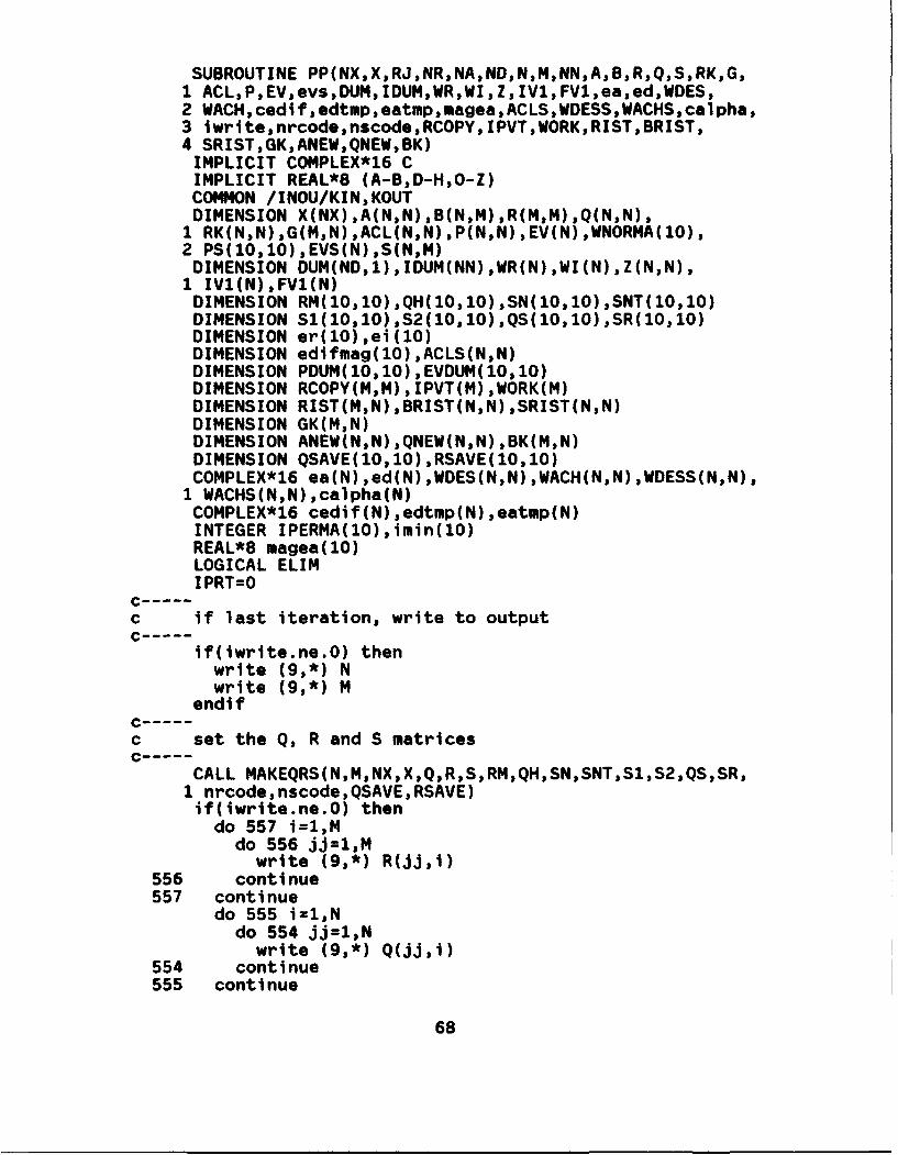
SUBROUTINE PP(NX,XRJ,NRNANDNMNNAsBRsQ,SRKG,1 ACL,P,EV,evsDUM,IDUM,WRWI,Z,IV1,FVI,ea,ed,WDES,2 WACH, cedif,edtmp,eatmp~mageaACLS,WDESSWACHS~calpha,3 iwrite~nrcode,nscodeRCOPY, IPVTWORKRIST,BRIST,4 SRISTsGKgANEW,QNEW$BK)IMPLICIT COMPLEX*16 CIMPLICIT REAL*8 (A-B2D-HjO-Z)COMMON /INOU/KINjKOUTDIMENSION X(NX),A(NN)sB(N3M),R(MM)sQ(NsN),1 RK(NsN)sG(M,N)sACL(NN),P(NN),EV(N)sWNORMA(10),2 PS(10,1O)qEVS(N)2S(NvM)DIMENSION DUM(ND,1),IDUM(NN),WR(N),WI(N),Z(NN),1 1V1(N)sFV1(N)DIMENSION RM(10,1O),QH(10,1O),SN(1091O)sSNT(10,1O)DIMENSION S1(lO,1O)sS2(10,1O),QS(1O,10O)SR(1O,10)DIMENSION er(10),ei(10)DIMENSION edifmag(10) ,ACLS(N,N)DIMENSION PDUM( 10910) ,EVDUM( 10210)DIMENSION RCOPY(MqM)qIPVT(M),WORK(M)DIMENSION RIST(M2N)*BRIST(NqN)tSRIST(N,N)DIMENSION GK(MvN)DIMENSION ANEW(NvN),QNEW(NgN),BK(M,N)DIMENSION QSAVE(10$10),RSAVE(1091O)COMPLEX*16 ea(N),ed(N),WDES(N,N),WACH(N,N),WDESS(N,N),1 WACHS(NN),calpha(N)COMPLEX*16 cedif(N),edtmp(N),eatmp(N)INTEGER IPERMA(10),imin(10)REAL*8 mageaC 10)LOGICAL ELIMIPRT=0

C ------

c if last iteration, write to output

if(iwrite.ne.0) thenwrite (9,*) Nwrite (9,*) M

endifC ------

c set the Q, R and S matricesC ------

CALL MAKEQRS(NgMNXXQRSRMQH,SNsSNTS1,S2,QSsSR,1 nrcode, nscodejQSAVE, RSAVE)if(iwrite.ne.O) thendo 557 i=1,M

do 556 jj=1,Mwrite (9,*) R(jj,i)

556 continue557 continue

do 555 i=19Ndo 554 jj=1,Nwrite (9,*) Q(jj,i)

554 continue555 continue

68

do 553 l.1,Mdo 552 jj=1,Nwrite (9,*) S(JJgi)

552 continue553 continue

endifC ------c calculate the lqr gain matrix, GKC ------

CALL TRNATB(NqM,NqMS2RIST)CALL SAVE(MxMM$MsRRCOPY)CALL MLINEQ(M,MsNRCOPYRIST,NCONDIPVT,WORK,l)CALL MMUL(N,MN,NsMqN2BtRIST,BRIST)CALL MMUL(NM,NNjMNqSRIST,SRIST)CALL MSUB(NNsNtN,NAqBRISTqANEW)CALL MSUB(N2NtNqN,NQSRIST,QNEW)CALL REG(NANRsNMsNN,ANEWB,QNEWR,RK,G,ACL,DUM,IDUM,1 IPRT)CALL MADD(MqM,MsMjN,GRISTOGK)if(iwrlte.ne.O) thendo 530 i=l,N

do 5555 jj=12Mwrite (9,*) GK(jj,i)

5555 continue530 continue

endifc -----c calculate the new closed loop eigenvaluesc -----

CALL MMUL(NtM2NsN,?4,N,B,GK,BK)CALL MSUB(NINvNjNxNA,BK,ACLS)ipc=1CALL EIGVV(NAs,NACLStWRWI,Z,IV1,FV1,IPCI1ERR)

c -----c count complex pairs and configure eigenvectorsc -----

i compl ex=Odo 539 i=19N

lf(WI(i).ne.O.Odo) icomplex=icomplex+1539 continue

NCMP=N- icompl ex/2I I=0do 540 i=19NCMP

ii=ii+1if(dabs(WI(ii)).gt.0.0) thendo 535 jj=1,N

WACH(jj ,ii)=DCMPLX( Z(jjii i)sZCjii ,l+))WACH(Jj ,Iii*1)=DCONJG(WAH ,jii))

535 continue11=11+1

elsedo 536 jj=l,N

WACH(jj,lii)=DCMPLX(Z(jj,ii ),0.OdO)

69

536 continueendif

540 continuecall WNORM(WACH,N)do 30 i=l,Nea(l )=dcmplx(WR(i ),WI(i))

30 continueC ------c write to output if final iterationC ------

40 continueif(iwrite.ne.0) thendo 43 i=lN

eareal=dreal (ea( i))ealmag=dlmag(ea( i))write (9,*) earealwrite (9,*) eaimag

43 continueendifdo 41 i1l,N

eatmp(i )=ea(i)edtmp( i)=ed(i)EVS(i)=EV(i)do 42 jj=l,N

WACHS(jj i )=WACH(jj~i)WDESS(Jjji )=WDES(jj~i)PS(jj Ii)=P(jj Ii)lf(iwrite.ne.0) thenwreal=dreal (wach(jj ,i))wimag=dimag(wach(jj, i))write (99*) wrealwrite (9s*) wimag

endif42 continue41 continue

iii =0do 501 jJ=1*N

do 502 kk=1,Nif(P(jj,kk).ne.0.OdO) jjj=jjj+1

502 continue501 continue

NL=NRJ=0.OdOdo 50 i=l,N

c -----c calculate difference between desired eigenvalues andc achievable elgenvalues. algorithm matches the closestc achieved elgenvalue to the desired eigenvalues, in thec order they were input.c -----

do 51 jj=1sNLcedif(jj )=edtmp(1)-eatmp(jj)

51 continue

70

do 56 jj=1*NLedifmag(jj )=dsqrt~dreal (cedif(jj) )**2+

+ dimag~cedif(jj))**2)56 continue

call imins(NL~edifmag,imin(i))iii=IMIN(i)RJVEC=0.OdOif(jjj.eq.0) then

if(iwrite.ne.O) thengoto 503

endifendif

C ------c calculate the calpha for the eigenvectorsc -----

suml= . OdOsum2=0.OdOif(dimag(eatmp(iii)).ne.0.OdO) then

do 584 jj=l,Nsumi = suml+dimag(WDESS(jj1l))

+ *dreal(WACHS(jj,iii))+ -dreal(WDESS(jj,l))*dimag(WACHS(jjiji))

sum2 = sum2+dreal(WDESS(jj,1))+ *dreal(WACHS(jj,iii))+ +dimag(WDESS(jj,1))*dimag(WACHS(jj,iii))

584 continuephl=datan2(suml,sum2)calphal=dcmplx(dcos(phl) ,dsin(phl))cal pha2=-l*cal phal

elsecalphal=(l.OdO,0.OdO)cal pha2=-l*cal phal

endi fc -----c determine which caipha produces minimum cost andc calculate eigenvector contribution to performancec indexc -----

DELWI 1=0. OdODELW12=0. OdO

do 585 jj=1sNDELWI1=PS(jj,l)*( (OREAL( WDESS(jj 4)-

4 calphal*WACHS(jj iii)) )**2+ +(DIMAG(WDESS(jj,l)-calphal+ *WACHS(jj,iii)))**2)+ +DELWI1

DELW12=PS(jj,l)*( (DREAL(WOESS(jj1l)-+ clh2WC j, ill)) )**2+ +(DIMAG(WDESS(jj1l)-calpha2+ *WACHS(jj,ill)))**2)+ +DELW12

585 continuelf(DELWI1.lt.DZLWI2) then

71

DEIWI =DELWI 1caiphal =calphal

elseDELWI =DELWI2cal phai =cal pha2

endifRJVEC=DELWIif (iwrite.ne.0) thendo 587 jj=l,N

if(eatmp(iii).eq.ea(jj)) calpha(jj)=calphai587 continue

if( i.eq.N)thendo 586 jj=1,N

alreal=dreal (calpha(jj))al imag=dimag(calpha(jj))

586 continueendif

endi f503 continue

c -----c add elgenvalue/elgenvector contribution to performancec indexc -----

RJ=RJ+EVS(1)*edifmag( iii )**2+RJVECc -----c reset the eigenvalue/vector arrays to eliminatec those poles already matched.c -----

k=0NL=NL-1do 52 jj=1,NL

k=k+1ELIM=jj .eq. iiiIF(ELIM) K=k+1eatmp(jj )=eatmp(k)edtmp(jj )=edtmp(jj+1)EVS(jj )=EVS(jj+1)if(jjj.eq.0) goto 591do 590 kk=l,N

WACHS(kk~jj )=WACHS(kk~k)WDESS(kk,jj )=WDESS(kksjj+l)PS(kk,jj )=PS(kk,JJ+1)

590 continue591 continue52 continue50 continue

RETURNEND

72

SUBROUTINE IMINS(NLsEOIF?4AGI)IMPLICIT REAL*8 (A-HqO-Z)DIMENSION EDIFMAG(NL)1=1do 5000 jj=l,nl

lf(dabs(edifmag(jj)).lt.dabs(edifmag(l))) l=jj5000 continue

returnend

73

SUBROUT INE WNORM (WVECq*N)IMPLICIT REAL*8 (A-HO-Z)DIMENSION WNORMV(1O)COMPLEX*16 WVEC(NqN)do 5 i=19NWNORMV(l )=0.OdO

5 continuedo 10 i=ltNdo 20 JJ=1,NWNORMV( I)=WNORMV( i)+(dreal (WVEC(JJ .1)) )**2+

+ (dimag(WVEC(jj3 i)))**220 continue10 continue

do 30 il=,Ndo 40 jj=1,N

WVEC jj )=WVEC(jj ,i )/dsqrt(wnormv( I))40 continue30 continue

returnend

74

SUBROUTINE MAKEQRS(NMNXsXQsRSRMQHsSNsSNT,51,52,1 QSsSRonrcodeanscodesQSAVEsRSAVE)IMPLICIT REAL*8 (A-HtO-Z)DIMENSION X(NX)sQ(NsN)vR(NM)qS(NjM)DIMENSION RM(MsM)sQH(NN)sSN(NsM),SNT(M,N)DIMENSION S1(NN),52(MM)sQS(N,M),SR(NsM),QSAVE(NN),DIMENSION RSAVE(M,M)

C ------c this subroutine reads the upper triangular portionc of matrices RMO QH and all of SN, if applicable, fromc X and returns Q, R and S matrices that meet thec constraints necessary for an LQR solutionc -----

ix=0if(nrcode.eq. 1.or.nrcode.eq.2) thenI x=1do 116 i=19M

do 117 jj=1,Mif(i.eq.jj) then

RM(i ,jj)=X(ix)else

RM(i ,jj )=O.OdOendif

117 continueif(nrcode.eq.2) ix=ix+1

116 continueelse

i count=0do 101 i=l,Mi count= icount+1do 102 jj=icount,M

ix=lx+1RM(i,jj)=Xix)RM(jj,i)=X(ix)

102 continue101 continue

endificount=0do 111 i=1,N

i count= icount+1do 112 jj=icount,Nix=ix+1QH(i,JJ )=X( ix)QH(jj,i )=X(ix)

112 continue111 continue

if(nscode.ne.0) thendo 131 ilsM

do 132 jj=19Mix=ix+1SN(jj,i )=X(ix)SNT(i,jj )=X( ix)

132 continue

75

131 continueendif

call NMUL(N2N2NqNjNqNQH9QHqQ)call Mt4UL(Mt,M,,M,M,M,RM,RM,R)

if(nscode.eq.O) thencall ZPART(N2N2MxS)

elsecall MMUL(N,MgSN,NMgNgSI4,SNT,S1)call MMUL(MNM 2MN,MISNT,SN,S2)call NMUL(N*NvNqNONjMsQHsSNaQS)call MMUL(NqMM,14Njt43MSNqRW4,SR)call SAVE(N2NqNsN,QSQSAVE)call MADD(NsN,NN,N$NQSAVEsS1qQ)call SAVE(M,M,MsM,R,RSAVE)call MADD(M2M,MqM,M2S2sRSAVE*R)call MADD(NSN2NxN2,QSqSRqS)

endifreturnend

76

ADDendix 0: Ooeratina Instructions

General

The following is provided as a guide for using the

included algorithm at AFIT. While the source code is

written in a standard FORTRAN language [24], the program

requires some special handling. Particularly, the specific

subroutines called upon in the program must be properly

accessed. The procedures presented here ensure proper use

of the program. The program is run on the Virtual Memory

System (VMS) cluster at AFIT. The cluster includes three

host computers: Hercules, Lancer and Sabre. Reference [25]

contains more details about the AFIT computer services.

The EIGSPACE source code is compiled using the FORTRAN

compiler on VMS. The object file is linked to the DLQGLIB

and IMSL subroutine packages. The DLQGLIB source code is

available at AFIT. For this project, the DLQGLIB object

file was placed in the same directory as the EIGSPACE

program. The IMSL subroutines must also be linked to the

algorithm. These routines are not available in FORTRAN at

AFIT. Following are the commands used to compile the

algorithm:

FORTRAN eigspace

LINK eigspace,dlqglib,imslibshare/opt

77

MATLABTO InteLCrfacej

The EIGSPACE program requires a single input file and a

single output file. Since most of the input and output are

expressed as matrices, MATLABT" provides a convenient

interface for the program. MATLABTM can be used as a stand

alone interface, via the LQREA.M file, which requires

interactive use of a terminal. The program can be more

efficiently run when submitted via the following command

file EIGSPACE.COM:

$run EIGSPACE$exit

The file, EIGSPACE.LOG is created which contains all screen

output data from the algorithm as well as other information

about the program execution. The LQRSAVE.M file is used to

create the input file for EIGSPACE, while the LQROUT.M file

is used to reformat the output file. The input and output

files should be in the same directory as the EIGSPACE file.

The m-files presented below ensure that the program will run

properly when MATLABTM is used in the same directory.

78

WOREA m-ile

function[QRSseagvaK]=LQREA(agbsedsFelvdFvstol,rcodesscodeskmax)

%LQREA Eigenstructure assignment using the Linear Quadratic%Regul ator.

%Form is [QqRjSqeaqvaqKJ=% ~LQREA(albgedsFe~vd,Fv,tol ,rcode,scode~kmax)

% Input parameters,% a,b~state space matrices of a linear system with n states% and m controls

% ed=nxn diagonal matrix of desired elgenvalues% Fe=nxl matrix weighting each eigenvalue% vd=nxn matrix whose columns are the desired eigenvectors

% (must be in same order as associated elgenvalues)% Fv=nxn matrix whose elements weight corresponding elements

% of vd% tol=convergence tolerance for performance index% rcode=(1) R=ro*I, (2) R=[diagj, (other) R=positive definite% scode=(O) S=nxm zero matrix, (other) S=control-state

% weights% kmax=maximum optimization iterations%Output parameters,% ea=nxn diagonal matrix of achievable eigenvalues% va=nxn matrix of achievable eigenvectors% QR,S=final state and control weighting matrices% K=gain matrix

(n~nc]=size(a);[mr~m]=size(b);

for i=1:n,edd(i ,1)=Fe( i);edd(i ,2)=real (ed(i I );edd (i ,3) =imag (ed ( i,i ));

endvdd( : ,)=Fv(:);vdd( :,2)=real (vd(:));vdd( : ,3) = imag (vd (:));save input.dat n at m bt edd vdd tol rcode scode kmax /ascii!run eigspaceload output.datcount=1;n=output(count);count=count+1;m=output(count);count=count+1;n2=n*n;m2=m*m;nm=n*m;

79

R=zeros~m,m);R( :)=output(count:count+m2-1);count=count+m2;Q=zeros(n~n);Q( :)=output(count:count+n2-1);count=count+n2;S=ones(n~m);SC: )=output(count:count+nm-1);count=count+nm;K=zeros(m,n)K( :)=output(count:count~nm-1)count=count+nmea=zeros(n~n);for 1=1:nea i *i )=output~count)+J*output(count+1);count=count+2;

endva=zeros(n~n);for jj=1:nfor i=1:nvaC iij)=output(count)+j*output(count+1);count=count+2;

endend

s0

LORSAVE 1-file

function LQRSAVE(absedFevdFvtol,rcodescode,kmax)%LQRSAVE saves all required data for the Eigenstructure%assignment algorithm using the Linear Quadratic Regulator.

% Form is LQRSAVE(ab,edFevdFvtolrcodescode)% Input parameters,

a,b = state space matrices of a linear system withn states and m controls

ed = nxn diagonal matrix of desired eigenvalues% Fe = nxl matrix weighting each eigenvalue

vd = nxn matrix whose columns are the desired% eigenvectors (must be in same order as

associated eigenvalues)% Fv = nxn matrix whose elements weight

corresponding elements of vd% tol = convergence tolerance for performance index

rcode = (1) R = pI% (2) R = [diag]

(3) R = positive definite% scode = (0) S=[O]

(1) S=control-state weightskmax = maximum optimization iterations

(n,ncl=size(a);[mr,mJ=size(b);at=a(:);bt=b(:)

for i=1:n,edd(l,1)=Fe(i);edd(i,2)=real(ed(i,i));edd(i,3)=imag(ed(i,i));

endvdd(:,l)=Fv(:);vdd(:,2)=real(vd(:));vdd(:,3)=imag(vd(:));save input.dat n at m bt edd vdd tol rcode scode kmax /ascii

81

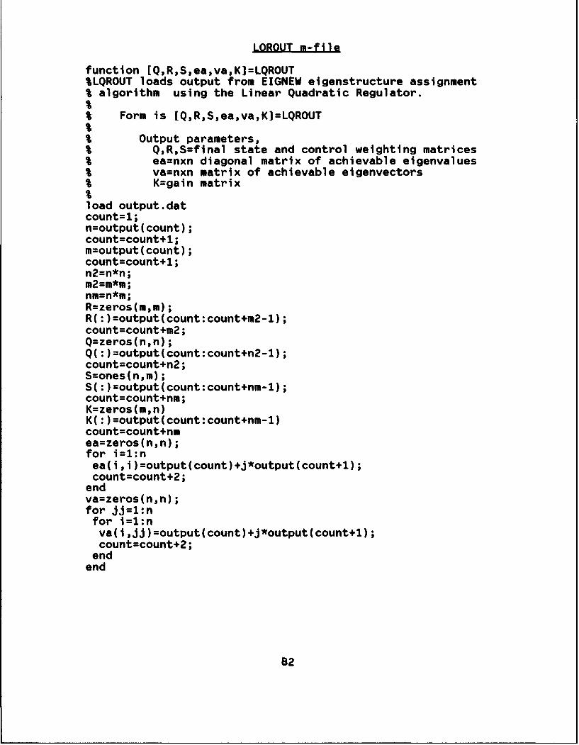
LOROUT rn-file

function [Q9RSea,va,KJ=LQROUT%LQROUT loads output from EIGNEW elgenstructure assignment% algorithm using the Linear Quadratic Regulator.

% Form is [QRqSjeajva,KJ=LQROUT

% Output parameters,% Q,RIS=flnal state and control weighting matrices% ea=nxn diagonal matrix of achievable elgenvalues% va=nxn matrix of achievable elgenvectors% K=gain matrix

load output.datcount=1;n=output(count);count=count+1;m=output(count);count=count+1;n2=n*n;m2=m*m;nm=n*m;R=zeros(m~m);R( :)=output(count:count+m2-1);count=count+m2;Q=zeros(n~n);Q( :)=output(count:count+n2-1);count=count+n2;S=ones(n~m);S : )=output(count:count+nm-1);count=count+nm;K=zeros(m~n)K( :)=output(count:count+nm-1)count=count+nmea=zeros(nn);for i=1:nea i, i )=output(count)+j*output(count+1);count=count+2;

endva=zeros(n.,n);for jj=1:nfor il1:nva(Iiij) =output(count)+J*output(count+1);count=count+2;

endend

82

Bi bl oraphy

1. Robinson, Jeffrey D. A Linear Ouadratlc ReaulatorWeiaht Selection Alaorithm for Robust Pole Assianment:MS Thesis. AFIT/GAE/ENG/9OD-23. School of Engineering,Air Force Institute of Technology, Wright-PattersonAFB, OH, December 1990.

2. Huckabone, Captain Thomas C. An Algorithm for RobustEiaenstructure Assignment Using the Linear OuadraticReaulator: MS Thesis. AFIT/GAE/91D-7. School ofEngineering, Air Force Institute of Technology, Wright-Patterson Air Force Base, Ohio, December 1991.

3. McRuer, Duane, Irving Ashkenas and Dunstan Graham.Aircraft Dynamics and Automatic Control. PrincetonUniversity Press, New Jersey, Princeton, New Jersey,1973.

4. Reid, J. Gary. Linear Systems Fundamentals: Continuousand Discrete. Classic and Modern. McGraw HillPublishing Company, New York, New York, 1983.

5. Tischler, M. B. Digital Control of Highly AuamentedCombat Rotorcraft. NASA Technical Memorandum 88346,May 1987.

6. Takahashi, M. D. A Flight-Dynamic HelicoDterMathematical Model with a Sinale FlaD-Laa-Torsion MainRotor. NASA Technical Memorandum 102267, February1990.

7. Helicooter Stability and Control. Flight Test ManualNo. 105, Naval Air Test Center, Patuxent River,Maryland, November 1983, Preliminary Edition.

8. Aeronautical Desian Standard. Handling QualitiesReauirements for Military Rotorcraft. ADS-33C, UnitedStates Army Aviation Systems Command, St. Louis,Missouri, August 1989.

9. Myers, Michael R., Freddie J. Mills, Floyd L. Dominick,Gary L. Skinner and R. Scott Mair. preliminar=Airworthiness Evaluation Prototype MH-60K HelicoDter(Handling Oualities). TECOM Report No. 4-CO-230-000-020, United States Army Technical Test Center, EdwardsAFB, California, August 1991.

10. Osder, Stephen and Donald Caldwell. "Design andRobustness Issues for Highly Augmented HelicopterControls," AIAA Guidance. Navioation and Control

nference, Volume 3, Session Paper No. 91-2751: pages1370-1380 (AUG 1991).

83

11. Operator's Manual. UH-60A and EH-60A Helicopter,Technical Manual TM-55-1520-237-10, United States ArmyAviation Systems Command, St. Louis, Missouri, January1988.

12. Garrard, William L. and Bradley S. Liebst. "Design ofa Multivariable Helicopter Flight Control System forHandling Qualities Enhancement," Journal of theAmerican Helicooter Society, Volume 35: pages 23-30(OCT 1990).

13. Moore, B. C. "On the Flexibility Offered by StateFeedback in Multivariable Systems Beyond Closed LoopEigenvalue Assignment," IEEE Transactions on AutomaticControl, Volume AC-21: pages 689-692 (OCT 1976).

14. Ridgely, D. Brett and Siva S. 3anda. Introduction toRobust Multivariable Control. AFWAL-TR-85-3102,Control Dynamics Branch, Flight Dynamics Laboratory,Wright-Patterson AFB, Ohio, February 1986.

15. MATLAB" User's Manual. The MathWorks, Inc., SouthNatick, Massachusetts, August 1988.

16. Floyd, Captain R. M. LOGLIB User's Manual: ADescription of Computer Routines for Use in LinearSystems Studies. School of Engineering, Air ForceInstitute of Technology, Wright-Patterson Air ForceBase, Ohio, May 1984.

17. IMSL User's Manual: Math/Library. IMSL, Inc., Houston,Texas, Volume 1, Chapters 1-2, Version 1.0 (APR 1987).

18. Kuester, James L. and Joe H. Mize. OptimizationTechnioues with FORTRAN. McGraw Hill Book Company, NewYork, 1973.

19. Anderson, Brian D. 0. and John B. Moore. OptimalControl. Linear Ouadratic Methods. Prentice Hall Inc.,New Jersey, 1990.

20. Strang, Gilbert. Linear Algebra and Its Applications,Harcourt Brace Jovanovich, San Diego, California, 1988.

21. Kreindler, Eliezer and Anthony Jameson. "Conditionsfor Nonnegativeness of Partitioned Matrices," IEEETransactions on Automatic Control, February 1972.

22. Safanov, Michael G. and Michael Athans. "Gain and PhaseMargin for Multiloop Regulators," IEEE Transactions onAutomatic Control, Volume AC-22: p. 173-1/9 (APR 1977)

84

23. Hoh, Roger, at Al. Prooosed Airworthiness DesianStandard: Handlina Oualities Reouirements for MilitaruRotorcrft. Technical Report no. 1194-2, SystemsTechnology, Inc., Hawthorne, California, December 1985.

24. VAX FORTRAN: Lanauaae Reference Manual. DigitalEquipment Corporation, Mynard, Massachusetts, June1988.

25. Introduction to AFIT Educational Computer Services, AirForce Institute of Technology, May 1991.

85

Vitn

Captain Dempsey D. Solomon was born on 9 July 1960 in

Dallas, Texas. He graduated from Mount Pleasant High School

in Mount Pleasant, Texas in 1978. He then attended the U.S.

Military Academy, at West Point, New York, graduating with a

Bachelor of Science degree in 1982. Captain Solomon was

commissioned into the U.S. Army in May 1982 as an Aviation

Logistics Officer. He completed rotary and fixed wing

flight training in January 1984. In 1988, Captain Solomon

completed the U.S. Naval Test Pilot School at Patuxent

River, Maryland. He served as an Experimental Test Pilot in

the U.S. Army Aviation Technical Test Center (USAATTC) at

Fort Rucker, Alabama and performed developmental testing on

UH-60A/L, CH-47D, OH-58D, AH-64A and non-standard fixed wing

aircraft. He has accumulated over 1800 flight-hours in 45

different aircraft during his career. Captain Solomon

completed his assignment at Fort Rucker as the Company

Commander at USAATTC prior to entering the School of

Engineering, Air Force Institute of Technology (AFIT), in

May 1991. Following graduation from AFIT, Captain Solomon

will be assigned to the 160th Special Operations Aviation

Regiment, 101" Airborne Division, at Fort Campbell,

Kentucky where he will serve as the Test Coordinator for the

U.S. Army's Special Operation's Aircraft program.

Permanent Address: 230 College Street

Pittsburg, Texas 75686

86

R DForm ApprovedREPORT DOCUMENTATION PAGE OMB No 0704-0188

Piulihc feoorting ouroen acr , irs ziection of .ntormation is estimated to a4eraqe I hour oer resooise, inctuding the time for reviewing instructions. searching exslting data sources,.gathering and maintining t!e z.ta needed, and conoieting and reviewmig the .ollection of nformation Send comments regarding this burden estimate or any other asoect Of thisccllection af intormatlon. •'c-•;ng suggestion% for reducing this ourden. to washington Headduarters Services. Directorate for information Doerations, and Reports, 1215 JeffersonsDavis H-iiway. Suite 1;C4. ,r, rqtcn. /A 22202-4302. and to "r'e Office of Management and 8uage'. Paoervfork Reduction Project (0704-0188). Washington. DC 20503.

1. AGENCY USE ONLY LLeave blank) 2. REPORT DATE 3. REPORT TYPE AND DATES COVERED

IDecember 1992 Master's Thesis4. TITLE AND SUBTITLE S. FUNDING NUMBERS

HELICOPTER FLIG14T CONTROL SYSTEMDESIGN USING TI7E LINEAR QUADRATIC REGULATOR FORROBUST EIGENSTRUCTURE ASSIGNMENT

6. -UTHOR(S)

Dempsey D. Solomon, Captain, USA

7. PERFORMING ORGANIZATION NAME(S) AND ADORESS(ES) 8. PERFORMING ORGANIZATIONREPORT NUMBER

Air Force Institute of Technology, AFIT/GAE/ENY/92D-17WPAFB OH 45433-6583

9. SPONSORING i MONITORING AGENCY NAME(S) AND AODRESS(ES) 10. SPONSORING/ MONITORINGAGENCY REPORT NUMBER

11. SUPPLEMENTARY NOTES

12a. DISTRIBUTION/ AVAILABILITY STATEMENT 12b. DISTRIBUTION CODE

Approved for public release;distribution unlimited

13. ABSTRACT (Maximum 200 words)

iTis thesis applies modern, multi-variable control design techniques, via aFORTRAN: computer algorithm, to U.S. Army helicopter models in hovering flightconditiuns. Eigenstructure assignment and Linear Quadratic Regulator (LQR)theory aie use, to achieve enhanced cjosed loop performance and stabilitycharacteristics with full state feedback. The addition of cross coupling weightsLu lhe standar'l LQR performance index is specifically addressed. A desiredeigenstiructure is chosen with a goal of reduced pilot workload via performancecharacteristics and modal decoupling consistent; with current helicopter handlingqualities requirements. Cross coupling weighting is shown to provide greaterflexibility in achieving a desired closed loop eigenstructure. While theaddition of cross coupling weighting is shown to eliminate stability marginguarantees associated with LQR methods, the modified algorithm can achieve acloser match to a desired eigenstructure than previous versions of the programwhile maintaining acceptable stability characteristics.

14. SUBJECT TERMS 15. NUMBER OF PAGES

Eigenstructure Assignment; Linear Quadratic Regulator; 96Cross Coupling; Helicopter Control Design 16. PRICE CODE

17. SECURITY CLASSIFICATION 18. SECURITY CLASSIFICATION 19. SECURITY CLASSIFICATION 20. LIMITATION OF ABSTRACT

UK ?W f ied ru0 a H91 f ied oWITT M f ied UL

NSN 7540-01-280-5500 Standard Form 298 (Rev 2-89)Prescribed by ANSI Std 139-182W1- 102