adaptive codes for physical-layer security · 2018-11-23 · adaptive codes for physical-layer...
TRANSCRIPT

FACULDADE DE ENGENHARIA DA UNIVERSIDADE DO PORTO
Adaptive Codes for Physical-LayerSecurity
João Paulo Patriarca de Almeida
Programa Doutoral em Telecomunicações
Orientador: Doutor João Francisco Cordeiro de Oliveira Barros, Professor Associadocom Agregação do Departamento de Engenharia Eletrotécnica e de Computadores da
Faculdade de Engenharia da Universidade do Porto
24 de Julho de 2014

c© João Paulo Patriarca de Almeida, 2014
Adaptive Codes for Physical-Layer Security
João Paulo Patriarca de Almeida
Programa Doutoral em Telecomunicações
Aprovado em provas públicas pelo Júri:
Presidente: Doutor José Alfredo Ribeiro da Silva Matos, Professor Catedrático da Facul-dade de Engenharia da Universidade do Porto
Arguente: Doutor Matthieu Bloch, Assistant Professor, School of Electrical and Com-puter Engineering, Georgia Institute of Technology, Atlanta, USA
Vogal: Doutor Mikael Skoglund, Associate Professor, School of Electrical Engineering,KTH Royal Institute of Technology, Stockholm, Sweden;
Vogal: Doutor Adriano Jorge Cardoso Moreira, Professor Associado do Departamento deSistemas de Informação da Universidade do Minho;
Vogal: Doutor Jaime dos Santos Cardoso, Professor Associado com Agregação do De-partamento de Engenharia Eletrotécnica e de Computadores da Faculdade de Engenhariada Universidade do Porto
28 de Maio de 2014


Dedicated to Inês, Aurora and to what the future holds.
In memory of Kika.
i

ii

Acknowledgments
The work presented in this thesis is a testament to how much I owe to my family, friendsand professors. The following lines will certainly follow short on acknowledging howdeeply grateful I am of being inspired by so many wonderful people.
First and foremost, a word to Prof. João Barros, the first responsible for having mestarted on this journey. From the moment we met, João put a high expectation on meand gave me the confidence to pursue any goals I was set out to reach. Among the manythings I could thank him for, I choose to thank him for his faith on my work and skills,for the freedom he gave me to work on any research topic I would fall in love with andfor always stimulating me with his curiosity and enthusiasm. It was indeed a pleasure toshare these last years with him.
Second, I would like to thank the committee members, Professors Matthieu Bloch,Mikael Skoglund, Adriano Moreira, Jaime Cardoso and José Matos, for their availabilityto be part of the defense jury, but mostly for allowing me to be part of a great discussionon physical-layer security.
I would also like to thank the opportunity given by Professor Matthieu Bloch andProfessor Muriel Médard for allowing me to spend some time with their research groups atGeorgia Tech Lorraine and MIT, respectively. The experiences have been both rewardingand fulfilling. Additional thanks to Professors Cristiano Torezzan and Willie Harrisonwho visited us in our lab and from whom I learnt so much!
While the journey to the Ph.D. was long and weary, all my colleagues from theNetworking and Information Security group at Instituto de Telecomunicações (IT-Porto)made it a lot more bearable. A salute to the groups former students João Vilela, Lu isaLima, Mate Boban and Sérgio Crisóstomo and best wishes for all of you who are waitingin line: Hana, João Rodrigues, Mari, Pedro, Rui Meireles, Saurabh and Susana.
I was fortunate enough to meet some of my best friends while working at NIS. Theyare role models in every aspect I can think about and will forever stay in my heart. Thankyou Diogo for your spirit, your enthusiasm, for letting me train my parenting skills withyou and for being always a great friend. Thank you minino Lato for having the patienceto teach me how to do research, for setting the bar so high and specially for sharing somany memorable and crazy moments, even those that we do not remember. Thank youPaulo, for always putting doubts in my mind with respect to anything possibly imaginable.While it was always a source of constant laughing, it made me revisit many things whichI would otherwise miss. To Rui, for always taking me back to the roots of greatness andreminding me never to settle for less. For sharing his passion for science and discoveryand the constant seek for elegance. To Tiago, for teaching me so many things and showingme that everything can be built from even the smallest example. For being a constantreference in principles and values that should always be a part of any scientist. To all
iii

iv
of you, I owe this thesis. Not only for the help you provided me with when I was stuckin technical details, but also for your faith in the problems I tackled and for the constantreminders of what we were set out to get when we all started this journey!
Of course that I am also in debt to many of my friends outside work. To all of you, mysincere thanks. A special thank you to Eliana, André, their daughter Mafalda and theirson Benjamim, for always reminding the values for which we should guide our lives withand for keeping in my mind that there is nothing more important than living fully, evenamong times where the hardest sacrifices are needed.
To my parents Vitorino and Belarmina, and my brother Zé , whose sacrifice, en-durance, guidance and example led me to finish this tough path. Without you support,it would be impossible to be who I am today.
Lastly, to my wife Inês and my daughter Aurora. We have taken huge steps these lastyears, suffered great losses, overcame many obstacles and built so many beautiful things.Last time I wrote down we were going to write many stories. Eventually we were able towrite the most beautiful fairy tale. Thank you for your infinite love and support. Thankyou for the endless joy I felt from the moment we met. For being my future.
With the greatest gratitude and love,
João Almeida

Resumo
Os sistemas de comunicação vêem tomando um papel cada vez mais importante nonosso dia-a-dia. O uso difundido da Internet e sistemas de comunicação sem fios não sóalteraram a forma como comunicamos, mas também o tipo de informação quecomunicamos. Dado que a maior parte do canais de comunicação são susceptíveis aescutas, e frequentemente é pretendida a transmissão de dados sensíveis, existe umaclara necessidade de mecanismos que garantam confidencialidade de comunicação.Tradicionalmente, a confidencialidade de dados é gerida na camada de aplicação, usandoprimitivas criptográficas. No entanto, nos últimos anos, outros métodos de segurançaforam desenvolvidos. Em particular, os métodos de segurança na camada física podemactuar como um complemento (ou alternativa) a soluções baseadas em criptografia. Deuma forma geral, a ideia subjacente a estas técnicas é a utilização do ruído inerente aoscanais de comunicação como fonte de aleatoriedade, um elemento essencial no desenhode sistemas de comunicação segura.O tópico fundamental desta tese é precisamente o desenvolvimento de esquemas desegurança para a camada física. Neste contexto, são exploradas várias alternativas aoestado-da-arte na construção de códigos seguros. Em particular, são fornecidasconstruções explícitas para fontes contínuas e discretas, com enfoque em códigos detamanho finito.Primeiro, é desenvolvido um quantizador escalar com restrições de segurança. A ideiaprincipal nesta construção é desenhar um código conjunto de fonte-canal que garantaque um atacante tenha uma distorção acima de um determinado limite. Tal objectivo éatingido usando um desenho cuidado dos parâmetros do quantizador escalar,nomeadamente as fonteiras de quantização e o número de níveis de quantização.Em seguida, é proposto o uso de mapeamentos de expansão de largura de banda paracanais de wiretap com ruído Gaussiano aditivo. Tais mapeamentos são caracterizadospela existência de erros anómalos, quando o ruído de canal se situa acima de um dadonível. Estes erros tipicamente levam a estimativas afectadas por uma grande distorção. Aideia aplicada na construção é desenhar um código que garanta que um atacante éafectado por erros anómalos com elevada probabilidade. Para isso, é usada umaconstrução denominada Torus Layer Spherical Codes, que permite um controle intuitivodo nível a partir do qual erros anómalos surgem.Finalmente, é proposto o uso de puncionamento aleatório como meio de obter segurançaem canais com apagamentos. O prícipio subjacente a esta construção é a interpretação datécnica de puncionamento aleatório como uma técnica de introdução de ruído artificial.Neste sentido, é possível utilizar o puncionamento aleatório para saturar o canal de umatacante com apagamentos, forando-o a operar com elevada equivocação. Duasinstâncias do sistema são consideradas. Primeiro é assumido que o padrão de
v

vi
puncionamento é público. Neste caso, a equivocação do atacante está directamenterelacionada com a sua capacidade de recuperar mensagens através de um canal deapagamentos, em que a probabilidade de apagamento é elevada. Num segundo caso, éassumido que o padrão de puncionamento é um segredo partilhado entre as entidadeslegítimas. Em particular, mostramos que o puncionamento aleatório introduz perdas desincronização ao nível do bit, contribuindo para um grande acréscimo à equivocação doatacante.

Abstract
Communication systems have taken an increasingly important role for most aspects ofour daily lives. The widespread use of the Internet and wireless communications not onlyhave changed the way in which we communicate, but also what type of information wecommunicate. Owing to the fact that most of the communication channels are open toeavesdropping, and often the data we wish to transmit is of a sensitive nature, it is clearthat mechanisms for ensuring confidential communications are required. Traditionally,confidentiality is managed at the application layer using cryptographic primitives.However, in recent years, other means of achieving confidential data transmission haveemerged. Physical-layer security is one of such techniques, which can act as acomplement (or sometimes alternative), to standard cryptographic solutions. Broadly, theidea of physical layer security is to use the noise inherent to communication channels asa source of randomness, an essential element to design secure communication systems.This thesis is fundamentally concerned with the development of security schemes for thephysical-layer. In this context, we explore several alternatives to current state-of-the-artsecrecy codes. In particular, we provide explicit code constructions for both continuousand discrete sources, focusing on codes with finite block-length.First, we develop channel-optimized scalar quantizers with secrecy constraints. Themain idea is to design a joint source-channel code which guarantees that theeavesdropper’s distortion lies above a prescribed threshold. This is achieved by a carefuldesign of the parameters of the scalar quantizer, most notably the quantizationboundaries and the number of quantizations levels.Second, we propose the use of bandwidth expansion mappings over wiretap Gaussianchannels. Bandwidth expansion mappings are characterized by the existence ofanomalous errors, when the channel noise is above a given threshold. These errorstypically lead to estimates of the transmitted messages with high distortion. The mainidea of the proposed code construction is to design codes such that the eavesdropper isgenerally affected by these anomalous errors. To this purpose we employ an instance ofspherical codes construction known as Torus Layer Spherical Codes, which allows for anintuitive control over the threshold above which anomalous errors appear.Finally, we propose the use of random puncturing as means to obtain secrecy for thebinary erasure wiretap channel. The underlying principle of the coding scheme is to lookat random puncturing as a technique for introducing artificial noise. Hence, we can userandom puncturing to saturate the eavesdroppers channel with erasures, forcing theeavesdropper to operate with high equivocation. Two instances of the system areconsidered. We first assume that the puncturing pattern is public. In this case theeavesdroppers equivocation is directly related to the ability of recovering messages froma binary erasure channel with a large erasure probability. We then move to the case
vii

viii
where the puncturing pattern is a shared secret between the legitimate parties. We showthat random puncturing introduces loss of bit-level synchronization, which contributes toa greater increase in the eavesdroppers equivocation.

Contents
1 Introduction 11.1 Two security models: computational and information-theoretic security . 31.2 Motivation . . . . . . . . . . . . . . . . . . . . . . . . . . . . . . . . . . 81.3 Outline and Main Contributions . . . . . . . . . . . . . . . . . . . . . . 10
2 Coding for Secrecy 132.1 The Wiretap Channel Model . . . . . . . . . . . . . . . . . . . . . . . . 132.2 Reliability and Secrecy Metrics . . . . . . . . . . . . . . . . . . . . . . . 15
2.2.1 Reliability Constraints . . . . . . . . . . . . . . . . . . . . . . . 152.2.2 Secrecy Constraints . . . . . . . . . . . . . . . . . . . . . . . . . 16
2.3 Fundamental Limits of Secure Communication . . . . . . . . . . . . . . 192.3.1 Weak and Strong Secrecy . . . . . . . . . . . . . . . . . . . . . 192.3.2 Weak Secrecy with Lossy Reconstruction . . . . . . . . . . . . . 202.3.3 Rate-Distortion Secrecy . . . . . . . . . . . . . . . . . . . . . . 21
2.4 Secrecy over the Wiretap Channel Model . . . . . . . . . . . . . . . . . 212.5 Practical Code Constructions for the Wiretap Channel . . . . . . . . . . . 252.6 Discussion . . . . . . . . . . . . . . . . . . . . . . . . . . . . . . . . . . 29
3 Scalar Quantization under Secrecy Constraints 333.1 Channel-Optimized Scalar Quantizers . . . . . . . . . . . . . . . . . . . 343.2 Scalar Quantizers under Security Constraints . . . . . . . . . . . . . . . 39
3.2.1 Problem Statement . . . . . . . . . . . . . . . . . . . . . . . . . 403.2.2 Overview of the optimization strategy . . . . . . . . . . . . . . . 413.2.3 Encoder Optimization . . . . . . . . . . . . . . . . . . . . . . . 433.2.4 Decoder Optimization . . . . . . . . . . . . . . . . . . . . . . . 51
3.3 Numerical Results . . . . . . . . . . . . . . . . . . . . . . . . . . . . . . 523.4 Discussion . . . . . . . . . . . . . . . . . . . . . . . . . . . . . . . . . . 56
4 Continuous Spherical Codes for Secrecy 594.1 Torus Layer Spherical Codes For Continuous Alphabets . . . . . . . . . . 61
4.1.1 Flat Tori . . . . . . . . . . . . . . . . . . . . . . . . . . . . . . . 624.1.2 Piecewise Torus Layer Spherical Codes . . . . . . . . . . . . . . 634.1.3 Decoding Errors . . . . . . . . . . . . . . . . . . . . . . . . . . 67
4.2 Piecewise Torus Layer Spherical Codes for Secrecy . . . . . . . . . . . . 684.3 Numerical Results . . . . . . . . . . . . . . . . . . . . . . . . . . . . . . 714.4 Discussion . . . . . . . . . . . . . . . . . . . . . . . . . . . . . . . . . . 74
ix

x CONTENTS
5 Randomly Punctured LDPC Codes for Secrecy 775.1 Randomly Punctured LDPC codes . . . . . . . . . . . . . . . . . . . . . 80
5.1.1 Encoding and Decoding of LDPC Codes over Binary ErasureChannels . . . . . . . . . . . . . . . . . . . . . . . . . . . . . . 81
5.1.2 LDPC Decoding Thresholds over Binary Erasure Channels . . . . 865.1.3 LDPC Decoding over Binary Deletion Channels with Erasures . . 89
5.2 Puncturing for Secrecy over the BEWC . . . . . . . . . . . . . . . . . . 915.2.1 Reliability . . . . . . . . . . . . . . . . . . . . . . . . . . . . . . 925.2.2 Secrecy . . . . . . . . . . . . . . . . . . . . . . . . . . . . . . . 925.2.3 Rate-Equivocation Regions . . . . . . . . . . . . . . . . . . . . . 94
5.3 Numerical Results . . . . . . . . . . . . . . . . . . . . . . . . . . . . . . 965.3.1 Asymptotic Performance with Public Puncturing Patterns . . . . . 965.3.2 Finite-Length Performance with Secret Puncturing Patterns . . . . 100
5.4 System Aspects . . . . . . . . . . . . . . . . . . . . . . . . . . . . . . . 1055.4.1 Sharing Secret Keys . . . . . . . . . . . . . . . . . . . . . . . . 1055.4.2 Secret Key Rates . . . . . . . . . . . . . . . . . . . . . . . . . . 1085.4.3 Comparison with the One-Time Pad Cryptosystem . . . . . . . . 108
5.5 Discussion . . . . . . . . . . . . . . . . . . . . . . . . . . . . . . . . . . 109
6 Conclusions 1116.1 Future Research . . . . . . . . . . . . . . . . . . . . . . . . . . . . . . . 112
A Basic Notions on Information Theory 115A.1 Information Sources . . . . . . . . . . . . . . . . . . . . . . . . . . . . . 115A.2 Entropy, Joint Entropy and Conditional Entropy . . . . . . . . . . . . . . 115A.3 Mutual Information and Conditional Mutual Information . . . . . . . . . 116A.4 I-measures . . . . . . . . . . . . . . . . . . . . . . . . . . . . . . . . . . 117A.5 Properties of Entropy and Mutual Information . . . . . . . . . . . . . . . 118A.6 Distortion . . . . . . . . . . . . . . . . . . . . . . . . . . . . . . . . . . 118
B Leakage Bound for Wiretap Codes 121
C Achievable Rate-Equivocation Region for the Wiretap Channel With a SharedKey 123
References 128

List of Figures
1.1 Example of asymmetric encryption. . . . . . . . . . . . . . . . . . . . . 31.2 Example of symmetric encryption. . . . . . . . . . . . . . . . . . . . . . 41.3 Physically degraded wiretap channel (DWTC) model. . . . . . . . . . . . 61.4 Broadcast channel with confidential messages (BCC). . . . . . . . . . . . 7
2.1 Wiretap channel model. . . . . . . . . . . . . . . . . . . . . . . . . . . . 142.2 Binning structure. . . . . . . . . . . . . . . . . . . . . . . . . . . . . . . 252.3 Nested code structure. . . . . . . . . . . . . . . . . . . . . . . . . . . . . 26
3.1 Communication system for transmission of continuous sources using witha joint source-channel code based on a scalar quantizer. . . . . . . . . . . 34
3.2 Example of thresholds and reconstruction values of two scalar quantizerswith n = 3 for a Gaussian source U ∼N (0,1). . . . . . . . . . . . . . . 38
3.3 Wiretap model for analog sources. . . . . . . . . . . . . . . . . . . . . . 393.4 Overview of optimization procedure. . . . . . . . . . . . . . . . . . . . . 423.5 SNR of legitimate receiver and eavesdropper for a channel optimized
scalar quantizer without secrecy constraints. The quantizer resolution isQ = 3 bits (8 levels). . . . . . . . . . . . . . . . . . . . . . . . . . . . . 53
3.6 SNR of legitimate receiver and eavesdropper for a scalar quantizer withsecrecy constraints when the main channel has a crossover probability ofδ = 10−5. The quantizer resolution is Q = 3. . . . . . . . . . . . . . . . 54
3.7 SNR of legitimate receiver and eavesdropper for a scalar quantizer withsecrecy constraints when the main channel has a crossover probability ofδ = 10−2. The quantizer resolution is Q = 3. . . . . . . . . . . . . . . . 55
3.8 SNR of legitimate receiver and eavesdropper for a scalar quantizer withsecrecy constraints for the degraded scenario. The quantizer resolution isQ = 3. . . . . . . . . . . . . . . . . . . . . . . . . . . . . . . . . . . . . 56
3.9 Number of levels of final quantizer design for the three wiretap instanceswhen ∆ = 0.3981. . . . . . . . . . . . . . . . . . . . . . . . . . . . . . . 57
4.1 Examples of 1:2 bandwidth expansion mapping. . . . . . . . . . . . . . . 604.2 Example of a mapping between the line [0,1] and curves over several tori. 624.3 Illustration of the encoding operations. . . . . . . . . . . . . . . . . . . . 664.4 Example of the decoding operations with the possible associated errors. . 684.5 Example of the impact of errors on the estimates of the source message. . 684.6 The AWGN wiretap channel model. . . . . . . . . . . . . . . . . . . . . 694.7 P(‖nb‖ ≤ d/2) and P(‖ne‖> d/2) as a function of distance d, for dimen-
sions n = 2 and n = 24. . . . . . . . . . . . . . . . . . . . . . . . . . . . 72
xi

xii LIST OF FIGURES
4.8 Map of parametrizations for which there exists a solution to the reliabilityand secrecy constraints with n = 2. . . . . . . . . . . . . . . . . . . . . . 73
4.9 P(‖nb‖ ≤ d/2) and P(‖ne‖> d/2) as a function of distance d, for dimen-sions n = 2,3,24 and 48. . . . . . . . . . . . . . . . . . . . . . . . . . . 75
5.1 Wiretap model of a coding scheme that uses puncturing to obtain secrecy.Two cases are considered: to the left the puncturing pattern is public,whereas to the right the the puncturing pattern is a shared secret betweenthe legitimate parties. . . . . . . . . . . . . . . . . . . . . . . . . . . . . 78
5.2 Operational interpretation of random puncturing, when the pattern is pub-lic (top figure) or secret (bottom figure). . . . . . . . . . . . . . . . . . . 79
5.3 Bipartite graph with n = 7 variable nodes (represented by circles) andn− k = 3 check nodes (represented by squares). . . . . . . . . . . . . . . 80
5.4 Example of a peeling decoder that is able to recover the transmitted code-word. . . . . . . . . . . . . . . . . . . . . . . . . . . . . . . . . . . . . 85
5.5 Example of a peeling decoder that is not able to recover the transmittedcodeword. . . . . . . . . . . . . . . . . . . . . . . . . . . . . . . . . . . 86
5.6 Maximum puncturing probability γ∗ as a function of the channel erasureprobability δ for the ensembles C1, C2 and C3 when using a BP and aMAP decoder. . . . . . . . . . . . . . . . . . . . . . . . . . . . . . . . . 98
5.7 Normalized equivocation rate for a publicly known puncturing pattern asa function of the wiretap channel erasure probability ε using a BP decoder. 99
5.8 Normalized equivocation rate for of a publicly known puncturing patternas a function of the wiretap channel erasure probability ε using a MAPdecoder. . . . . . . . . . . . . . . . . . . . . . . . . . . . . . . . . . . . 99
5.9 Rate-equivocation region and achievable rate-equivocation pairs for theensembles C1, C2 and C3, when using the largest admissible puncturingprobabilities for varying values of ε . . . . . . . . . . . . . . . . . . . . . 101
5.10 Equivocation rate for the legitimate receiver for codes C1, C2 and C3 withblock-length n = 12 as a function of the main channel erasure probability δ .102
5.11 Normalized equivocation rate for the eavesdropper for codes C1, C2 andC3 with block-length n = 12, as a function of the wiretap channel era-sure probability ε . The considered puncturing probabilities γ are equal toεMAP, γ1 and γ2. . . . . . . . . . . . . . . . . . . . . . . . . . . . . . . . 103
5.12 Rate-equivocation regions of the considered models and the rate-equivocationpairs for codes C1, C2 and C3 for both the asymptotic and finite block-length case. Wiretap model parameters are δ = 0 and ε = 0.25. . . . . . . 104
5.13 Simulated average bit error rate for the code C4 as a function of the wire-tap channel erasure probability ε , when the main channel erasure proba-bility takes values from δ ∈ {0,0.1,0.25}. . . . . . . . . . . . . . . . . . 106
5.14 Simulated average bit error rate for the code C5 as a function of the wire-tap channel erasure probability ε , when the main channel erasure proba-bility takes values from δ ∈ {0,0.1,0.25}. . . . . . . . . . . . . . . . . . 106
5.15 Bounds on the equivocation of simulated error probability for the code C4as a function of the wiretap channel erasure probability ε , when the mainchannel erasure probability takes values from δ ∈ {0,0.1,0.25}. . . . . . 107

LIST OF FIGURES xiii
5.16 Bounds on the equivocation of simulated error probability for the code C5as a function of the wiretap channel erasure probability ε , when the mainchannel erasure probability takes values from δ ∈ {0,0.1,0.25}. . . . . . 107
5.17 Shannon Cipher System with erasures. . . . . . . . . . . . . . . . . . . . 109

xiv LIST OF FIGURES

List of Tables
2.1 Examples of secrecy criteria . . . . . . . . . . . . . . . . . . . . . . . . 182.2 Comparison of code families . . . . . . . . . . . . . . . . . . . . . . . . 29
3.1 Performance of Lloyd-Max and channel-optimized scalar quantizers for aBSC(δ ) . . . . . . . . . . . . . . . . . . . . . . . . . . . . . . . . . . . 38
4.1 Performance of spherical codes for the wiretap channel with n = 2. . . . . 73
5.1 Equivalence of rate-equivocation regions as a function of the disclosurestrategy and nature of the puncturing pattern. . . . . . . . . . . . . . . . 95
5.2 Degree distributions of LDPC code ensembles C1, C2 and C3. . . . . . . . 975.3 Puncturing probabilities of LDPC code ensembles C1, C2 and C3 with
prescribed level of equivocation. . . . . . . . . . . . . . . . . . . . . . . 1005.4 Degree distributions for the LDPC code ensembles C4, and C5. . . . . . . 105
xv

xvi LIST OF TABLES

Notation
X Alphabet or setpX Probability distribution of XX ∼ pX Random variable X follows distribution pXpX |Y Conditional probability distribution of X given YEX Expected value over XH(X) Entropy of XH(X |Y ) Conditional entropy of X given YI(X ;Y ) Mutual information between X and Y0,1n Binary vector of length nR Field of real numbersF Galois Fieldλ Lagrangian multiplier∇ Gradient functionN (µ,σ2) Gaussian distribution with mean µ and variance σ2
‖n‖ Norm of vector nS1 Sphere in the Euclidean spaceδSB Distance between folds in a curveδT Distance between two tori
xvii

xviii Notation

Abbreviations
AWGN Additive White Gaussian NoiseBCC Broadcast Channel with Confidential MessagesBER Bit error rateBDC Binary Deletion ChannelsBEC Binary Erasure ChannelBEWC Binary Erasure Wiretap ChannelBP Belief PropagationBSC Binary Symmetric ChannelCO-SC Channel-Optimized Scalar QuantizerCSI Channel State InformationCSNR Channel Signal-to-noise RatioKKT Karush-Kuhn-TuckerLDPC Low-Density Parity CheckLM-SC Lloyd-Max Scalar QuantizerMAP Maximum a PosterioriML Maximum LikelihoodMSE Mean Square ErrorMMSE Minimum Mean Square ErrorOPTA Optimum Performance Theoretically AchievablePDF Probability Density FunctionSC Spherical codesSK Shannon-Kotel’nikovSNR Signal-to-noise RatioTLSC Torus Layer Spherical CodesWTC Wiretap Channel ModelWTC-SK Wiretap Channel Model with a Shared Key
xix

xx Abbreviations

Chapter 1
Introduction
Devising schemes for secret communications has been an object of study almost since theinvention of the first alphabets. In ancient civilizations, where the first forms of encryptionappeared, they were mostly used to create an aura of mystery around messages written intombstones [1]. However, they soon became an essential tool for military purposes acrossthe ages. The ability to encrypt (or hide) the contents of messages was a crucial advan-tage in preparing field operations, as well as for secret diplomatic communication [1]. Onthe other hand, the competence on performing cryptanalysis, i.e., the ability to break anencryption scheme and obtaining the respective contents of a hidden message, became aneven greater advantage, as it revealed plans and information from adversaries, allowing toproperly adopt any necessary counter-measures. While in the past the arts of cryptographyand cryptanalysis where mostly restricted to the domain of military and diplomatic com-munications, the evolution of computer networks has changed this paradigm, establishingsecurity as a ubiquitous concern.
In modern communication systems, entities interact using devices as proxies and com-munication takes place through channels that may be remotely eavesdropped/tampered.Such outline suggests a broad scope of security concerns [2]. For instance, communicat-ing entities should be able to corroborate the identity of each other, which implies somesort of mechanism should provide for identity authentication. Users should be able tocorroborate the source of a given received message, as well as being able to verify if thatmessage have not been subject to changes. Therefore, mechanisms that guarantee mes-sage authentication and data integrity are imperative. It could also be the case that theorigin or reception of a given message needs to be proven, for which schemes that ensurenon-repudiation are required. Another relevant question is how to prevent unauthorizedusers from accessing some resource, which could be tackled with appropriate access con-trol mechanisms. These examples illustrate some of the security objectives that should bemet, if required by the communicating entities. Notwithstanding the emergence of thesenew security concerns, data confidentiality is still one of the most crucial security prob-
1

2 Introduction
lems. In general, it is not possible to guarantee that the messages transmitted from somedevice will not be observed by an unintended third party. This fact is even more evidentin wireless networks since wireless transmissions are by nature susceptible to eavesdrop-ping [3, Chapter 5], where intercepting messages (which may contain sensitive data) canbe done with any device equipped with a wireless interface. Such eavesdropping attacksare categorized as a passive attacks [4, Chapter 1.3]1. Clearly, solutions are required toensure that unauthorized entities (or eavesdroppers) are not able to decipher the contentsof a captured message.
Within the context of modern communication networks, cryptography is extensivelyused as the standard technique to achieve data confidentiality. In particular, for networksorganized in a layered architecture, it is common to find suites of security protocols (basedon principles of modern cryptography) that provide confidentiality services for many net-work layers. One such example is the Internet protocol suite, which proposes the use ofconfidentiality mechanisms at the application, transport and network layers for the en-cryption of raw data, the payload of TCP/UDP packets and the payload of IP packets,respectively. Surprisingly, the physical layer is often neglected as a layer where securitymechanisms should be implemented, even though it is ultimately the layer responsiblefor transmitting data (e.g. modern radio-based communication systems do not implementdata confidentiality at the physical-layer, but at layers above). Moreover, it provides anatural source of randomness (the communication channel), an essential ingredient ofany secrecy system. A possible justification lies on the fact that cryptographic-based so-lutions have reached a seemingly mature state. This contrasts with existing solutions thatuse the physical-layer to achieve security, which are still in an early stage of development.In addition, cryptographic solutions are not constrained by the type of source message andhave only a small set of requirements (e.g. the existence of an encryption key). Schemesthat exploit the benefits provided by the physical-layer tend to make several assumptionswith respect to the source and the underlying communication channel, which may behard to guarantee in practice. Consequently developing practical schemes with sufficientabstraction and generality for security purposes at the physical layer is not a simple pro-cess. However, in recent years, remarkable progress has been made both in the theoryand practice of physical-layer security. Consequently, it is anticipated that these schemeswill eventually achieve a state of maturity that allows their adoption on standard commu-nication systems. The main topic of this thesis is precisely this: the design of practicalsecurity schemes for data confidentiality based on physical-layer security principles.
1While active attacks such as jamming might have severe consequences, they are in general easier to detect andappropriate counter-attack measures can be taken. On the other hand, passive attacks such as eavesdropping are almostimpossible to detect. Consequently, one should pro-actively implement mechanisms that prevent eavesdroppers fromacquiring any meaningful information, rather than to react to eavesdropping events.

1.1 Two security models: computational and information-theoretic security 3
Alice Encryption
Kpub
Decryption
Kpriv
Bob
Eve
M C M
Figure 1.1: Example of asymmetric encryption.
1.1 Two security models: computational and information-theoreticsecurity
The motivation behind this thesis will be more evident once we contrast the virtues andlimitations of the computational security model and the information-theoretic securitymodel (under which physical-layer security is based2).
Algorithms based on the computational security model rely on problems that are com-putationally hard to solve unless some side information is available to the user. Thesealgorithms are based on the assumption of the existence of one-way functions [5, Chap-ter 2], i.e. functions that are easy to compute (given a function f and an input x, thereexists a polynomial-time algorithm that computes f (x)) but hard to invert (for a possibleinput x, the average probability of successfully finding an inverse of x under f for anyprobabilistic polynomial-time algorithm is negligible) [5, Chapter 2]. Thus, the essenceof the computational security model lies on considering an adversarial model where themalicious user has limited computational resources.
A broad class of primitives that fall in this domain are based on the concept of asym-metric cryptography (also known as public-key cryptography). A typical setup for public-key encryption/decryption is illustrated in Fig. 1.1. In this class of algorithms, users areequipped with a private/public key pair (Kpriv,Kpub). They distribute their public keys,which are then used to encrypt messages that are destined to them. Once they receive anencrypted message, they use the private key to decrypt the transmitted cipher-text. Essen-tially, the key pair should be constructed in such a way that trying to obtain the privatekey from the public key requires to solve a hard problem (e.g. trying to invert a one-wayfunction). The RSA [6] and ElGamal [7] cryptosystems are natural examples of publickey cryptography. One possible attack on the RSA public key encryption scheme can
2The difference between information-theoretic security and physical-layer security is subtle but exists. The formeris generally concerned with the characterization of the secrecy of a system, based on information theoretic quantities,and does not necessarily assume the existence of a communication channel. On the other hand, physical-layer securitybases itself on the information-theoretic security model to provide secrecy at the physical-layer.

4 Introduction
Alice Encryption Decryption Bob
Eve
K
M C M
Figure 1.2: Example of symmetric encryption.
be performed by solving the problem of prime factorization while an attack on the El-Gamal public key encryption scheme can be performed by solving the discrete logarithmproblem [8]. Both of these problems are believed to be one-way functions, and thereforehard to solve. Generally, the implementation of these primitives requires computationallyexpensive operations such as computing exponentiations and moduli. Therefore, thesestrategies are often used to share a single secret which will act as a key to a more compu-tationally efficient (albeit generally less secure) symmetric-key encryption algorithm. Insymmetric encryption algorithms, the same key is used both for encryption and decryp-tion operations (see Fig. 1.2). Therefore, such key should be shared a priori (e.g. throughthe public-key cryptography framework described above). Symmetric ciphers make useof the principles of confusion and diffusion proposed by Shannon [9]. Confusion refersto creating a complex relationship between the cipher-text C and the secret key K whilediffusion refers to creating a complex relationship between the message M and the cipher-text C3. Ultimately, these ciphers create an avalanche effect where changing one bit ofeither the message or the secret key leads to a cipher-text that is independent of the orig-inal cipher-text, which makes the system hard to attack. On the other hand, this alsomakes it vulnerable to channel noise, since the decryption of a cipher-text contaminatedwith errors will lead to decoding the wrong message.
Given the properties of the systems based on public-key/symmetric-key cryptography,it is not surprising that they have been largely adopted in current communication systems:they are reasonably efficient, data agnostic and apparently secure under the premise oflimited computational resources. Indeed, the existence of one-way functions is not yetmathematically proven [5, Chapter 2] (essentially proving the existence of such functionswould prove that the complexity classes P and NP are not the same, a long-standing prob-lem in theoretical computer science). Even if this is the case, such functions may onlybe applied under the correct computational model (e.g. the problem of factoring largeintegers can be solved in polynomial time in a quantum computer [11]). Thus, the longterm security of these schemes cannot be ensured if, for instance, quantum computers
3The most common way to implement these principles is to use substitution-permutation networks of Feistel net-works [10].
1.1 Two security models: computational and information-theoretic security 5
become ubiquitous. Aside from the security notions, modern ciphers also present somepractical concerns. It is not uncommon that these ciphers suffer from broken implemen-tations which, in practice, means that these schemes can be attacked through alternativemeans. For instance, [12] lists several attacks that can be performed on the RSA cryp-tosystem that range from the wrong choice of parameters for key generation and partialkey exposures to timing/power attacks or attacks based on faulty computations. Theseconcerns are sufficient for at least considering the possibility of using a different securityparadigm.
Information-theoretic security provides an alternative formulation of the secrecy prob-lem. The field was born in Shannon’s landmark paper in 1949 [9] as a natural extensionof information / communication theory. The basic problem in information theory is torecover a message that is transmitted over a noisy channel with an arbitrarily small error.In information-theoretic security one needs not only to ensure the aforementioned con-dition for the legitimate party, but also that a malicious third party (eavesdropper), withaccess to the transmitted messages, possibly corrupted by channel noise, cannot reduceits uncertainty about the transmitted message. More precisely, if a user wishes to transmita secret message M, encoded as C, the average uncertainty of the information obtained bythe eavesdropper can be measured using the conditional entropy H(M|C). This quantityis also commonly denoted as the eavesdropper’s equivocation. If H(M|C) = 0, there isno uncertainty left in the information obtained by the eavesdropper, which means that hisobservation provides him with sufficient information to obtain M without any errors. Onthe other hand, if H(M|C) =H(M), the eavesdropper’s average uncertainty about M is thesame with or without C. Hence, the captured message does not provide any informationto the eavesdropper. A system that ensures H(M|C) = H(M) is called unconditionallysecure or perfectly secure. Such systems are immune to cryptanalysis [9].
The first aspect to be retained is that an information-theoretic formulation of secrecyprovides a precise definition/measure of security. The second aspect is that assumptionsregarding the resources available to the eavesdropper do not need to be made.
Shannon originally worked on an information-theoretic formulation of symmetric en-cryption, where the eavesdropper observes an error-free cryptogram (as in Fig. 1.2). Heshowed that communicating under unconditional security constraints is only possible ifthe entropy of the key is greater or equal than the entropy of the message [9]. This resultimplies that the key of a symmetric encryption scheme should be at least as large as theoriginal message. Eventually, if a key with such characteristics is not available to thelegitimate party, they will have to share it over a possibly unsecured channel. Hence, theproblem of how to communicate the key over an insecure channel remains, which may beeven harder to solve than the original problem. On the other hand, it also shows that sym-metric ciphers based on small secret keys (used in many current systems) cannot ensureunconditionally secure communications, suggesting that such strategies may not be strong

6 Introduction
Alice EncoderMain
ChannelDecoder Bob
WiretapChannel
Eve
M Xn Y n M
Zn
Figure 1.3: Physically degraded wiretap channel (DWTC) model.
enough to provide for secrecy. However, these pessimistic results are a consequence ofthe strict assumptions of the communication model, since the only available source ofrandomness is the secret key.
Inspired by Shannon’s formulation, Wyner [13] contemplated the use of a differentsource of randomness, the communication channel. He proposed a new model for se-crecy, which is now commonly known as the wiretap model [13]. Rather than giving theeavesdropper a noiseless copy of the cipher-text, Wyner assumed that the eavesdropper’sobservations were obtained through a channel that is corrupted by noise. The first wiretapmodel considered that the eavesdropper’s observations were (physically) degraded ver-sions of the messages obtained by the legitimate receiver (see Fig. 1.3). Additionally,Wyner relaxed Shannon’s conditions for unconditionally secure communication. Insteadof requiring that the eavesdropper’s equivocation is equal to the source’s entropy, Wynerproposed the use of equivocation rate as a secrecy metric, in which case it is required thatthe eavesdropper’s equivocation rate is arbitrarily close to the entropy rate of the source,i.e. 1
nH(M|Zn) ≈ 1nH(M), for sufficiently large n. Then, he defined the secrecy capacity
as the maximum rate that satisfies such condition, while ensuring that the error probabilityof the legitimate receiver is arbitrarily small.
Wyner’s model implicitly assumed that the eavesdropper has access to degraded ver-sions of the messages received by the legitimate receiver, and therefore enforces a verystrict assumption with respect to the eavesdropper’s observations. Csizár and Körner [14]generalized the degraded wiretap model to account for a broadcast channel from thesource to the legitimate receiver and the eavesdropper. This model, illustrated in Fig. 1.4,can be thought of as a system with two parallel channels: one between the sender and le-gitimate receiver (main channel) and another between the sender and eavesdropper (wire-tap channel). Furthermore, [14] extends the wiretap model in the following way: sourcemessages have a private and public component. The private message M1 is to be decodedonly by the legitimate receiver and the public message M0 is to be decoded by both thelegitimate receiver and the eavesdropper. While both wiretap models contrast in a fewaspects, the imposed reliability and secrecy constraints are very similar. However, therate-equivocation region and secrecy capacity characterizations are more complex in thelatter case.
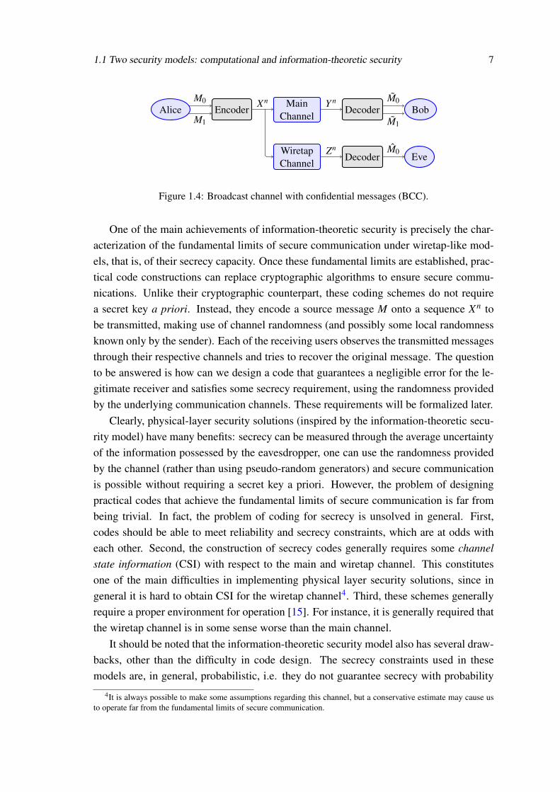
1.1 Two security models: computational and information-theoretic security 7
Alice EncoderMain
ChannelDecoder Bob
WiretapChannel
Decoder Eve
M0
M1
Xn Y n M0
M1
Zn M0
Figure 1.4: Broadcast channel with confidential messages (BCC).
One of the main achievements of information-theoretic security is precisely the char-acterization of the fundamental limits of secure communication under wiretap-like mod-els, that is, of their secrecy capacity. Once these fundamental limits are established, prac-tical code constructions can replace cryptographic algorithms to ensure secure commu-nications. Unlike their cryptographic counterpart, these coding schemes do not requirea secret key a priori. Instead, they encode a source message M onto a sequence Xn tobe transmitted, making use of channel randomness (and possibly some local randomnessknown only by the sender). Each of the receiving users observes the transmitted messagesthrough their respective channels and tries to recover the original message. The questionto be answered is how can we design a code that guarantees a negligible error for the le-gitimate receiver and satisfies some secrecy requirement, using the randomness providedby the underlying communication channels. These requirements will be formalized later.
Clearly, physical-layer security solutions (inspired by the information-theoretic secu-rity model) have many benefits: secrecy can be measured through the average uncertaintyof the information possessed by the eavesdropper, one can use the randomness providedby the channel (rather than using pseudo-random generators) and secure communicationis possible without requiring a secret key a priori. However, the problem of designingpractical codes that achieve the fundamental limits of secure communication is far frombeing trivial. In fact, the problem of coding for secrecy is unsolved in general. First,codes should be able to meet reliability and secrecy constraints, which are at odds witheach other. Second, the construction of secrecy codes generally requires some channelstate information (CSI) with respect to the main and wiretap channel. This constitutesone of the main difficulties in implementing physical layer security solutions, since ingeneral it is hard to obtain CSI for the wiretap channel4. Third, these schemes generallyrequire a proper environment for operation [15]. For instance, it is generally required thatthe wiretap channel is in some sense worse than the main channel.
It should be noted that the information-theoretic security model also has several draw-backs, other than the difficulty in code design. The secrecy constraints used in thesemodels are, in general, probabilistic, i.e. they do not guarantee secrecy with probability
4It is always possible to make some assumptions regarding this channel, but a conservative estimate may cause usto operate far from the fundamental limits of secure communication.

8 Introduction
one but rather with arbitrarily high probability. While this does not constitute a problemper se, care should be taken when specific codes are employed since they may not providethe level of secrecy one was expecting. Furthermore, the security notions are asymptoticby definition. Since any implementation of a physical-layer security system requires theuse of finite block-lengths, one should proceed with caution when moving from codeconstructions based on asymptotic analysis to the finite block-length regime.
In summary, security schemes based on the information-theoretic model may provideseveral benefits over schemes based on the computational model, either in terms of mea-surable secrecy and computational efficiency (secrecy is obtained via coding, which isalready implemented in any communication system for reliability purposes). However, italso has some disadvantages which may not be neglected such as strict assumptions onchannel models or the need to restrict the transmission rate to account for secrecy. Thatbeing said, it is certainly true that such schemes could be used to enhance the securityat the higher layers of the protocol stack. For instance, physical-layer security schemescan be coupled with cryptographic schemes and guarantee that, with high probability, anadversary will have access to a cipher-text that contains errors [16]. Clearly, the task of acryptanalyst is made harder since cryptographic attacks are generally designed under theassumption of a correct cipher-text. They can also simplify the task of key distribution,since they do not require a secure channel a priori. One can use the principles of physical-layer security to develop key agreement schemes based on the fact that an eavesdropperreceives a signal that is different from the legitimate receiver [17]. Both these aspectssuggest that a cross-layer approach to secrecy may be desirable in many cases. Alongthese lines, physical-layer security can be useful to enhance the security levels of currentsystems or to simplify the design of secrecy systems. This represents a departure fromthe complex security architectures that are currently employed, which make use of thirdparties for key distribution. It also provides the means to effectively assess the security ofa system, by filling the lack of secrecy metrics that currently exists.
1.2 Motivation
While the problem of coding for secrecy under the information-theoretic model is stillunsolved in general, code designs that achieve secrecy capacity are in fact known. Manypractical code constructions have been developed under the notion of weak secrecy pro-posed by Wyner [13]. Most of these code constructions share the same guideline, whichis to map every message to possible multiple codewords and randomly choose a messagewithin this set for transmission [15]. This principle can be put into practice using codeswith a nested structure, where a codebook is partitioned onto several sub-codebooks, eachone associated with a message to be transmitted. When the transmitter wishes to send a
1.2 Motivation 9
given message m, he randomly selects a message m′ from the sub-codebook that is as-sociated with m and transmits it. A sufficient condition to guarantee weak secrecy is todesign the sub-codebooks to be capacity-achieving over the wiretap channel [3, Chapter6]. Due to this seemingly simple constraint, nested codes became the prevailing practicalcode construction for physical-layer security. Consequently, most of the research effortson coding for physical-layer security focus on finding codes, based on nested structures,that satisfy this condition.
While useful from a theoretic and practical perspective, the application of nested codescan be limited by the operational environment [15]. These constructions have severalrequirements, some of which we list next. First, codes must have an arbitrarily largeblock-length. Second, channel state information (CSI) for the main and wiretap channelis required to properly dimension the codebook. Third, the code is dependent on suchchannel state information. The following observations, connected to these requirements,motivate the need for alternative code designs for secrecy:
• In any communication system the employed codes must have a finite block-length.This remark has several ramifications: a) source-channel separation theorems maynot hold, meaning that the optimal coding scheme for a communication systemcould involve solving a joint source-channel coding problem; b) the secrecy per-formance of a code may be far from the performance predicted by its asymptoticanalysis; and c) the objective of achieving secrecy capacity becomes unreachablewhich may justify using alternative secrecy metrics.
• While legitimate users may cooperate in order to characterize their communicationchannel, it may be very hard to obtain the CSI for the wiretap channel in practice.Therefore, code constructions should provide a good secrecy performance either fora large range of channel parameters or, if some estimate of the quality of the wiretapchannel is available, under the circumstances of channel mismatch.
• Depending on the communication environment, it may be the case that channelstatistics vary over time. Since codes with nested structures vary the sizes of theirsub-codebooks according the main and wiretap channel statistics, a change in chan-nel condition may imply the design of a new code. Consequently, nested codes maybe unfit for time-varying channels.
The code designs proposed in this thesis attempt to circumvent the aforementionedissues. More precisely, the proposed code constructions are of finite block-length. Con-sequently, the secrecy analysis associated with these codes will reflect this fact. A keypoint is that the proposed codes do not strive to achieve the secrecy capacity, but ratherensure that the eavesdropper’s ability to estimate the sent messages is greatly impaired.We do require that this impact can be quantified through information theoretic quantities.

10 Introduction
However, the secrecy criteria employed on the eavesdropper’s side may not necessarily bethe eavesdropper’s equivocation, but could be, for instance, distortion. A second aspectis that the proposed codes are deterministic. This contrasts with the common approachused to design secrecy codes, which considers the use of stochastic encoders through in-stances of local randomness. The reason is that stochastic encoding is useful to cancel outthe information leaked to the eavesdropper, but this requires CSI for the wiretap channel.Therefore, if such information is not available, it is not clear how to use the local ran-domness at the encoder to satisfy the secrecy constraints. Thus, our general approach tothe problem of code design for secrecy focuses on meeting a certain reliability constraintwhile providing a best-effort approach with respect to secrecy. While deterministic con-structions generally have a worse performance (in terms of secrecy) when compared tostochastic codes, they allow for a simplified design which is sufficient for the purposes weintend (design codes that provide a prescribed level of security for a large range of chan-nel parameters). We do note that the proposed schemes can also be extended to includenested-like structures. Finally, we distinguish code constructions according to the type ofsource. We consider two types of sources: a) sources that are discrete in time and contin-uous in amplitude (herein referred as continuous sources) and b) sources that are discretein time and amplitude (herein referred as discrete sources). While there exists a largebody of research that addresses discrete sources, secrecy codes for continuous sourcesare almost non-existent5. The reason lies in the fact that, if source-channel separationtheorems hold, the secrecy capacity may be achieved by using an optimal source encoderfollowed by an optimal wiretap code, and hence secrecy is achieved on the discrete partof the problem [18]. As mentioned before, these arguments may not hold and even ifthey do, both components may be extremely hard to design, thus motivating a differentapproach to the design of secrecy codes for continuous sources.
1.3 Outline and Main Contributions
In this thesis we propose three coding schemes for the problem of confidential data trans-mission. The first two schemes are directed towards continuous sources, while the thirdfocuses on discrete sources. Within the domain of continuous sources we propose a joint-source channel coding scheme based on scalar quantizers and a coding scheme based onbandwidth expansion mappings. The objectives in each of these constructions are distinct.The former construction forces eavesdroppers to operate bellow a desired performance
5Continuous sources arise in many situations. Audio and video signals can be represented by continuous variablesthat are subject to digitalization prior to transmission. The coefficients of Fourier and other related transforms are alsogenerally represented by continuous variables. For instance, the discrete cosine transform (DCT), that is widely used inimage coding standards, outputs real-valued coefficients. Signal processing techniques make ample use of continuousrandom variables (filtering, signal acquisition, ...). Additionally, natural sources (e.g. the quantities measured by asensor) or artificially induced sources (e.g. sources induced from channel gains) can be represented by continuousvariables. Thus, many applications could benefit from secure coding schemes that operate over continuous alphabets.

1.3 Outline and Main Contributions 11
threshold while the latter tries to ensure that the eavesdropper is bound to operate in aregime of anomalous errors, which greatly impacts the distortion of his estimates. Withinthe domain of discrete sources we propose a scheme based on randomly punctured LDPCcodes. The scheme uses puncturing as a mechanism to introduce artificial noise to createa saturated channel from the eavesdropper’s perspective. It also tries to explore the lack ofbit-level synchronization at the eavesdropper’s side to obtain higher secrecy gains. Thisis accomplished by allowing the puncturing pattern to be secret. The scheme also takesadvantage of the fact that rate-compatible codes enable the adaptation of codes to channelconditions, without the need to design a new code.
The main contributions of this thesis are as follows.
• Scalar Quantization under Secrecy Constraints: We propose a joint source-channel coding approach to secrecy that is based on solving an optimization prob-lem. The main idea is to find a joint source-channel code that minimizes the dis-tortion at the legitimate receiver, subject to a distortion constraint on eavesdropper.The process involves finding the boundaries of a scalar quantizer as well as find-ing the optimal index assignment (channel code) that satisfies the above constraints.Our results demonstrate that such an approach can effectively bound the distortionat which the eavesdropper can operate, even when the channel to the eavesdropperis better than that of the legitimate receiver.
• Piecewise Torus Layer Spherical Codes for Secrecy: We propose code construc-tions for the transmission of continuous sources without the need for quantization.The main technique employed is the transmission of curves over several layers oftorus, which are obtained via spherical codes. By exploiting the geometrical proper-ties of this construction, we find the code parameters which, with a desired probabil-ity, ensure decoding errors at the eavesdropper’s end that induce a large distortion.The construction has the additional advantage of transmitting messages over a di-mension that is double the dimension of encoding and decoding. This feature canbe used to obtain higher secrecy gains since the noise affecting the eavesdropperpossesses more components.
• Randomly Punctured LDPC Codes for Secrecy: We propose a coding schemebased on the principles of rate-compatible codes, where random puncturing is usedto adapt both to the channel conditions as well as for secrecy purposes. We considertwo scenarios: 1) the puncturing pattern is publicly known and 2) the puncturingpattern is a shared secret between the legitimate parties. We analyze the equivo-cation rate achieved by LDPC codes when the legitimate receiver has access to abelief propagation (BP) decoder or a maximum a posteriori (MAP) decoder. Ourresults indicate that using public puncturing patterns while allowing MAP decoding

12 Introduction
leads to maximum equivocation for the eavesdropper (albeit at an increase in termsof rate - which prevents us from achieving perfect secrecy), while only allowing BPdecoding results in a smaller equivocation for the eavesdropper but also a smallertransmission rate. Finally, it is shown that if the puncturing pattern is a shared se-cret, it is possible to achieve high equivocation rates for the eavesdropper, even forvery small block-lengths. The effort to share the puncturing pattern depends onthe puncturing probability. Hence, for large enough puncturing probabilities, therequired secret rate can be deemed small.
The rest of this thesis is organized as follows. Chapter 2 introduces more formallythe wiretap model, its fundamental limits and the state of the art in coding for secrecy. InChapter 3 we present a methodology for the design of scalar quantizers with secrecy con-straints that bound the performance achieved by an eavesdropper. We pose the problem ofsecrecy as a constrained optimization problem and derive necessary conditions for locallyoptimal encoders and decoders (under a mean square error distortion criterion). We thenpresent numerical results highlighting the distortion behaviour of the eavesdroppers opti-mal estimates under several scenarios. Bandwidth expansion mappings are introduced inChapter 4, as well as a particular construction of these mappings that is based on mappinga source onto a set of curves over several layers of tori. We provide a characterizationof the different types of errors that may occur in such construction. Then, assuming themain and wiretap channels are additive white Gaussian noise (AWGN), we use the geo-metrical properties of these codes to characterize the error probabilities associated witheach type of error. Using these probabilities, we find the code parameters that ensurethe eavesdroppers will suffer from the decoding errors that induce a distortion of largestmagnitude. We then present several numerical results that relate to the code parame-ters, as well as the distortion behaviour of the eavesdropper. Chapter 5 addresses thedesign of randomly punctured LDPC codes. We present wiretap channel models that takepuncturing into account, derive the eavesdropper’s equivocation under these models andcharacterize their rate-equivocation regions. We also derive bounds on the allowed punc-turing probabilities based on the code’s thresholds. We characterize the eavesdropper’smaximum likelihood decoder and present simulation results for specific code instancesbased on the derived decoder. We further present numerical results with respect to theeavesdropper’s equivocation rate, in particular asymptotic results for public puncturingpatterns and finite block-length results for secret puncturing patterns. Chapter 6 presentsthe conclusions of this thesis, discussing several directions for future work.
Chapter 2
Coding for Secrecy
In this chapter we will introduce some of the notions regarding the theory and practiceof secrecy systems based on the information-theoretic security model. We assume fa-miliarity with the basic definitions and results from information theory. For the sake ofcompleteness, a necessary set of results that are used in this thesis are summarized inAppendix A. We will first formally introduce the definitions of wiretap channel and wire-tap code, followed by possible definitions of reliability and secrecy constraints. We thenmove towards the characterization of the fundamental limits of secure communication un-der some of these constraints. We also review the design of state-of-the-art wiretap codesbased on nested structures.
2.1 The Wiretap Channel Model
The basic problem we wish to solve is how to transit some source message to a legiti-mate receiver that is able to correctly decode such message while keeping it secret fromunintended recipients. Thus, we wish to solve a communication problem with two con-straints: a reliability constraint for communication between the legitimate party and asecrecy constraint with respect to the eavesdropper’s observations.
In the context of physical-layer security, this problem can be modelled using the so-called wiretap channel model, illustrated in its generalized form in Fig. 2.1. It incorporatesthree users: a sender (Alice), a legitimate receiver (Bob) and an eavesdropper (Eve). BothBob and Eve receive the messages transmitted by Alice through a broadcast channel,which comprised of two parallel channels. The channel from Alice to Bob is called themain channel, while the channel from Alice to Eve is called the wiretap channel. Forsimplicity, we will assume throughout this thesis that both channels are memoryless andthe noise is assumed to be independent for Bob and Eve. It is also possible to considerthe case where noise the main and wiretap channels do not have independent noise. Inthese cases, one generally obtains less secrecy, reason for which one should try to use
13

14 Coding for Secrecy
Alice Encoder PY n|Xn(yn|xn) Decoder Bob
PZn|Xn(zn|xn) Eve
M Xn Y n M
Zn
Figure 2.1: Wiretap channel model.
alternative techniques such as interleaving in the attempt to create independent channels.Formally, the wiretap channel can be defined as follows.
Definition 1 (Wiretap channel). A wiretap channel (X , Y , Z , pY Z|X(y,z|x)) is character-ized by a quadruple that consists of one input alphabet X , two output alphabets Y and Zand a transition probability matrix pY Z|X(y,z|x).
As noted in Section 1.1, secrecy can be ensured through coding. Hence, to commu-nicate over the wiretap channel, Alice chooses a message M that she wishes to securelytransmit to Bob. She then encodes this message onto the channel input vector Xn usingsome wiretap code. Through the main channel, Bob observes a possibly noisy codewordY n, while Eve observes also a possibly noisy codeword Zn through the wiretap channel.Since the main and wiretap channel are memoryless, we have that
pY nZn|Xn(yn,zn|xn) =n
∏i=1
pY Z|X(yi,zi|xi).
The wiretap code is responsible for ensuring that reliable and secure communication ispossible. By reliable it should be understood that Bob can reproduce the source messagewith negligible error, while by secure it should be understood that Eve’s estimates of thesource message are erroneous. How one can exactly measure the reliability and secrecyperformance of a particular code will be briefly addressed. Let us first formally introducewiretap codes. A (discrete) wiretap code can be defined as follows.
Definition 2 (Discrete wiretap code). A (2nR, n) code Cn for a wiretap channel consists of
• A countable message setM= [1, . . . ,2nR];
• An encoding function (possibly stochastic) f : M→X n, mapping source messagesonto channel codewords;
• A decoding function g : Yn→M∪{?}, mapping channel observations to the sourcemessage set or an error message.

2.2 Reliability and Secrecy Metrics 15
Note that the wiretap code needs to introduce sufficient redundancy so that the legit-imate user is able to decode the messages without any errors. This redundancy also pro-vides the eavesdropper useful information. Therefore, allowing the encoder to be stochas-tic is essential to achieve full secrecy. The introduced randomness provides the means tocancel some information leakage that may occur while using a particular codebook fortransmission. On the other hand, as discussed before, unless we have some knowledgeabout the wiretap channel, it is not clear how one can use this randomness. This problemcan be circumvented by designing deterministic secrecy codes, which simply rely on therandomness provided by channel. They do incur in some information leakage, and there-fore do not achieve full secrecy. However, if codes are carefully designed, such leakagemay be small enough that no meaningful information can be extracted from it.
2.2 Reliability and Secrecy Metrics
Recall that our main objective is to design coding schemes that allow two parties to com-municate reliably, while preventing an eavesdropper from acquiring any meaningful in-formation about the transmitted messages. Thus, as mentioned earlier, the system shouldguarantee two constraints: a reliability constraint and a secrecy constraint. Such con-straints may take many forms, although ultimately they aim at the following general goals:an admissible (preferably negligible) error probability for the legitimate party (reliability)and statistical independence between the transmitted messages and the eavesdropper’sobservations (secrecy). The reason why statistical independence is relevant from a secu-rity perspective is that it reduces the best attack strategy of an eavesdropper to randomguessing.
2.2.1 Reliability Constraints
The most common measure used for reliability is the average error probability of thewiretap code
Pe(Cn) , Pr{M 6= M|Cn}, (2.1)
which measures the average probability that the legitimate receiver estimates the wrongmessage. In the discrete case, Pe(Cn) amounts to
Pe(Cn) =1d2nRe
d2nRe
∑m=1
Pr{m 6= m|Cn}. (2.2)

16 Coding for Secrecy
Commonly, we wish that legitimate parties communicate with negligible error. Then,the reliability constraint to be satisfied is formulated as
limn→∞
Pe(Cn) = 0. (2.3)
However, it may be the case that the average error probability is hard to analyze fora given wiretap code. Alternative metrics can be used in such cases, like the average bit-error rate (BER) [19, 20]. The BER is an approximate estimate of the bit error probability,thus capturing a similar idea to the average error probability. The reliability constraint canbe defined in a similar manner to (2.3), by requiring that BER for the legitimate receiverto approach zero in the limit of large block-lengths.
Finally, distortion can also be used to characterize the reliability of a wiretap code. Adistortion formulation of the problem of secure communication was provided in [18] andextended in [21]. The main motivation was to understand how allowing a prescribed levelof distortion for the legitimate receiver could provide a positive impact on the secrecy ofthe system. The reliability constraint to be satisfied can be formulated as
E{d(M,M)} ≤ D+ ε, (2.4)
where E denotes expectation, d(·, ·) is a distortion function and D is the prescribed level ofdistortion. The formulation of reliability is terms of distortions bears an additional chal-lenge, which is to find an appropriate distortion measure, that reflects the cost of choosingthe representation of the source message by its reconstruction point. For instance, forsome sources squared error distortion may be a good candidate, while for others not.
The choice of a particular measure for reliability does not require an extensive jus-tification. As noted before, the general requirement is a vanishing error probability, beit in any type or form. However, the choice of a particular measure for secrecy shouldcertainly be more judicious.
2.2.2 Secrecy Constraints
The first information-theoretic secrecy metric, introduced by Shannon [9], was uncondi-tional security, also known as perfect secrecy. To obtain perfect secrecy exact statisticalindependence1 is required with respect to the source message and the eavesdropper’s ob-servation. Assuming the wiretap code Cn is known to all parties, perfect secrecy is definedas follows.
H(M|Zn) = H(M) (2.5)
1We note that statistical independence could be measured in terms of any distance between joint probability distri-butions. In this thesis we focus on the Kullback-Leibler divergence, which is equivalent to the mutual information.

2.2 Reliability and Secrecy Metrics 17
or alternatively
I(M;Zn) = 0. (2.6)
Systems that provide perfect secrecy have demanding constraints which in practice arevery hard to meet. To circumvent this issue, it is possible to relax the secrecy constraint.Rather than requiring exact statistical independence between M and Zn, consider the caseof asymptotic statistical independence. The secrecy constraint then becomes
limn→∞
I(M;Zn) = 0. (2.7)
This constraint is commonly referred as strong secrecy and implies that the total amountof information leaked to the eavesdropper goes to zero as the size of the codewords goesto infinity. While the strong secrecy constraint is less restrictive than perfect secrecy,designing codes for the strong secrecy constraint is still very challenging.
Most practical code constructions adopt an even less restrictive constraint. Instead ofrequiring a total leakage of zero, they require the leakage rate to the eavesdropper to bevanishing, as the size of the codewords goes to infinity. This constraint can be formalizedas follows.
limn→∞
1n
I(M;Zn) = 0. (2.8)
It should be noted that the same coding rates are achievable under the strong and weak se-crecy constraints [22], although current coding schemes still incur in rate losses to ensurestrong secrecy [23].
All of the above criteria depend on the ability to analyze the equivocation of Cn. Insome cases, most notably when Cn is a code of finite block-length, it may be hard to ex-actly analyze the code’s equivocation. To circumvent this issue, several researchers haveadopted the code’s average error probability or the bit error probability as a secrecy crite-rion. In such cases, it is required that the eavesdropper’s estimates of the source messagesuffer from an arbitrarily high error probability (or alternatively the error probability isbounded above a prescribed threshold). This secrecy formulation was used to analyzethe secrecy of punctured LDPC codes [19] or lattice codes [24] over Gaussian wiretapchannels. The analysis of the secrecy constraint is simplified by using density evolutiontechniques in the former case and geometrical arguments on the latter.
We stress that error based metrics do not guarantee secrecy in an information-theoreticsense, i.e. a high error-rate does not imply a high equivocation. That being said, the error-rate could, in fact, be a pointer to the secrecy performance of a particular code. Moreover,since the equivocation of a code can be bounded with respect to the decoding error [25],this constitutes an alternative way to find codes that may be interesting from a secrecy

18 Coding for Secrecy
perspective.
Alternatively, it is also possible to use distortion as a secrecy measure. In particular,in [26, 27] the authors have considered a distortion-based approach where the goal isto characterize the fundamental limits of communication when we have a bound for theminimum average distortion for the eavesdropper (which they term as payoff ). If, fromZn, the eavesdropper produces an estimate M of the source message M, such secrecycriterion can be cast as
E{d(M,M)} ≥ D− ε, (2.9)
where E denotes expectation, d is a distortion function and D is the minimum distortionallowed at the eavesdropper. This formulation becomes particularly useful for continuoussources, since it is more amenable to analysis than differential entropy. However, itssecrecy interpretation is different to a large extent. Rather than measuring the amountof information obtained by the eavesdropper, it measures its ability to correctly estimatethe source messages. Therefore, it requires the assumption of some decoder, which mayunderestimate the amount of information collected by the eavesdropper. That being said,it also offers some advantages. For instance, a distortion metric is able to connect theperceptual quality to the secrecy metric (under a proper choice of distortion function).
The secrecy obtained through the error-rate and distortion formulations is sometimesreferred to as partial secrecy.
A summary of the described secrecy criteria is provided in Table 2.1.
Table 2.1: Examples of secrecy criteria
Secrecy Goal Constraint
Perfect Secrecy exact statistical independence I(M;Zn|Cn) = 0
Strong Secrecy asymptotic statistical independence limn→∞
I(M;Zn|Cn) = 0
Weak Secrecy asymptotic statistical independence limn→∞
1n I(M;Zn|Cn) = 0
Partial SecrecyNon-decodability E{Pe(Cn)} ≈ |M|−1
|M|
Bounded error-rate E{Pe(Cn)} ≥ Pmine
Bounded distortion E{d(M,M)} ≥ D− ε
It is possible to establish an ordering relationship between the secrecy metrics basedon the distance between probability distributions [28]. In particular, perfect secrecy isstronger than strong secrecy which is stronger than weak secrecy [28]. Such orderingimplies that a metric satisfying a stronger secrecy criterion also satisfies a weaker one.Such ordering is not completely clear with respect a distortion based approach, sincethere exists a dependency on the choice of distortion function [26].
2.3 Fundamental Limits of Secure Communication 19
A final comment is in order with respect to the secrecy metrics. While it is obviouslypreferable to choose a secrecy metric that is as strong as possible, at this point in time,such choice bears an impact in the code design, be it in terms of rate, delay or complexity.Therefore, for a given application, one should in fact choose a secrecy metric that allowsus to trade-off all these quantities while providing a desirable secrecy level. For instance,a streaming application may only require that the distortion of the eavesdropper is highenough to affect is perceptual quality. This would allow an increase in the transmissionrate for the legitimate party that could reduce its own distortion (when compared to a morestrict secrecy constraint).
2.3 Fundamental Limits of Secure Communication
The notions of reliability and secrecy defined above can be used to establish the funda-mental limits of secure communication. These limits answer the question of what is thelargest rate at which we can communicate under a given reliability and secrecy constraint(i.e. the secrecy capacity). It is possible to combine any of the criteria presented above.However, we will restrict our attention to the most common characterizations.
2.3.1 Weak and Strong Secrecy
Weak and strong secrecy have a similar characterization. A system is said to operate withweak secrecy if it satisfies conditions (2.2) and (2.8), while a system is said to operatewith strong secrecy if it satisfies conditions (2.2) and (2.7). The following definitions areneeded for the definition of the weak secrecy capacity.
Definition 3 (Weak rate-equivocation pair). A weak rate-equivocation pair (R, Re) is saidto be achievable for the wiretap channel if there exists a sequence of (2nR, n) codes Cn
such that:
1. limn→∞
Pe(Cn) = 0;
2. limn→∞
1nH(M|Zn)≥ Re.
Definition 4 (Weak rate-equivocation region). The weak-rate equivocation region of awiretap channel is given by the closure of all the achievable weak rate-equivocation pairs(R, Re), i.e.
RWTC , closure ({(R,Re) : (R,Re) is achievable}). (2.10)

20 Coding for Secrecy
Definition 5 (Weak secrecy capacity). The weak secrecy capacity of a wiretap channel isgiven by the supremum of all the achievable weak rate-equivocation pairs (R, Re), suchthat R = Re, i.e.
CWTCs , sup
R{R : (R,R) ∈ RWTC}. (2.11)
To define the strong secrecy capacity we need the following definition.
Definition 6 (Strong rate-equivocation pair). A strong rate-equivocation pair (R, Re) issaid to be achievable for the wiretap channel if there exists a sequence of (2nR, n) codesCn such that:
1. limn→∞
Pe(Cn) = 0;
2. limn→∞
H(M|Zn)≥ Re.
Then, the definition of the achievable strong rate-equivocation region and strong se-crecy capacity are equal to Def. 4 and Def. 5 where the (R, Re) pairs are strong rate-equivocation pairs.
2.3.2 Weak Secrecy with Lossy Reconstruction
If some distortion is allowed at the side of the legitimate receiver, we can provide a rate-distortion formulation to the weak secrecy problem using conditions (2.4) and (2.8). Inthis case, we can extend the previous definition of achievable rate to account for lossyreconstruction.
Definition 7 (Weak rate-equivocation pair with lossy reconstruction). A weak rate-equivocationpair (R, Re) with lossy reconstruction parameter D is said to be achievable for the wiretapchannel if there exists a sequence of (2nR, n) codes Cn such that:
1. liminfn→∞
E{d(M,M)} ≤ D+ ε;
2. limn→∞
1nH(M|Zn)≥ Re.
Then, it is possible to define the admissible region rate-distortion-equivocation regionand find the largest rate at which we can communicate under weak secrecy that satisfiesour rate-distortion constraint.

2.4 Secrecy over the Wiretap Channel Model 21
2.3.3 Rate-Distortion Secrecy
The above formulation relaxes the reliability constraint, but we may also relax the se-crecy constraint by conditioning the eavesdropper to operate under a distortion constraint(rather than equivocation or equivocation rate). The following formulation is particularlyuseful when sources are continuous. Using constraints (2.4) and (2.9) we can define thefollowing pair.
Definition 8 (Rate-distortion pair). A rate-distortion pair (R, D) with lossy reconstructionparameter D is said to be achievable for the wiretap channel if there exists a sequence of(2nR, n) codes Cn such that:
1. liminfn→∞
E{d(M,M)} ≤ D+ ε;
2. limsupn→∞
E{d(M,M)} ≥ D− ε;
2.4 Secrecy over the Wiretap Channel Model
The definitions provided before allow us to perform suitable choices when we wish touse physical-layer security schemes. Depending on the application at hand we may wishenforce a strict secrecy policy or choose to trade-off reliability and/or secrecy for rate.Moreover, depending on the type of source, one might prefer choosing a certain criterionover other criteria. This can only be accomplished if we are able to characterize thesefundamental limits.
For the general wiretap channel introduced in 2.1 the weak rate-equivocation regionand weak secrecy capacity are as follows.
Theorem 1. ([14],[3, Corollary 3.3]) Consider a wiretap channel (X , Y ,Z , pY Z|X(y,z|x)).For any joint distribution pUV X on U ×V ×X that factorizes as pU pV |U pX |V , define theset RWT (pUV X) as
RWT (pUV X) =
{(R,Re) :
0≤ Re ≤ R≤ I(V ;Y )0≤ Re ≤ I(V ;Y |U)− I(V ;Z|U)
}.
Then, the weak rate-equivocation region for this wiretap channel is the convex set
RWT =⋃
pUV X
RWT (pUV X). (2.12)

22 Coding for Secrecy
Corollary 1. ([14], [3, Corollary 3.4]) The weak secrecy capacity of the discrete memo-ryless broadcast wiretap channel is
CWTs = max
pV XI(V ;Y )− I(V ;Z).
The above characterizations introduce two auxiliary random variables U and V . Theyboth relate to the wiretap channel as follow: U relates to the information decodable byBob and Eve while V relates to the encoder randomization. Hence, it is not strange that Udoes not appear in the characterization of the secrecy capacity, since we wish Eve to obtainno information at all. While general, such characterization fails to give a strong intuitionwith respect to how randomization can affect secrecy without solving the associated max-imization problem, which in general is a arduous task. Fortunately, this characterizationcan be simplified for certain classes of channels, notably those that can be characterizedby an explicit advantage.
Definition 9 (Physically degraded channel). A channel (X , Z , pZ|X ) is said to be physi-cally degraded with respect to a channel (X , Y , pY |X ) if, for all triples (x,y,z) ∈ X ×Y×Z , pY Z|X(y,z|x) factorizes as pZ|Y (z|y)pY |X(y|x), i.e. if X →Y →Z .
Definition 10 (Stochastically degraded channel). A channel (X , Z , pZ|X ) is said to bestochastically degraded with respect to a channel (X , Y , pY |X ) if there exists a channelpZ|Y (z|y) such that, for all tuples (x,z) ∈ X ×Z , pZ|X(z,x) can be written as pZ|X(z,x) =∑
y∈YpZ|Y (z|y)pY |X(y|x), i.e. if the channel (X , Z , pZ|X ) has the same marginal distribution
as a channel that is physically degraded w.r.t (X , Y , pY |X ).
Definition 11 (Noisier channel). A channel (X , Z , pZ|X ) is said to be noisier than achannel (X , Y , pY |X ) if, for every V such that V → X→ (Y,Z), we have I(V ;Y )≥ I(V ;Z).
Definition 12 (Less capable channel). A channel (X , Z , pZ|X ) is said to be less capablethan a channel (X , Y , pY |X ) if, for every input X , we have I(X ;Y )≥ I(X ;Z).
Using the above definitions, we refer to degraded wiretap channel when a wiretapmodel is comprised of a wiretap channel that is physically or stochastically degraded w.r.tthe main channel. Likewise, we refer to noisier wiretap channel when a wiretap modelconsists of a wiretap channel that is noisier than main channel and by less capable towiretap model where the wiretap channel is less capable than main channel.
For the degraded wiretap channel, the weak rate-equivocation region and weak secrecycapacity can be characterized as follows.

2.4 Secrecy over the Wiretap Channel Model 23
Theorem 2. ([14], [3, Theorem 3.2]) Consider a wiretap channel (X , Y ,Z , pY Z|X(y,z|x))such that the wiretap channel is physically or stochastically degraded w.r.t the main chan-nel. Define the set RWT (pX) as
RWT (pX) =
{(R,Re) :
0≤ Re ≤ R≤ I(X ;Y )0≤ Re ≤ I(X ;Y )− I(X ;Z)
}.
Then, the weak rate-equivocation region for this wiretap channel is the convex set
RWT =⋃pX
RWT (pX). (2.13)
Corollary 2. ([14], [3, Corollary 3.1]) The weak secrecy capacity of the physically orstochastically degraded wiretap channel is
CWTs = max
pXI(X ;Y )− I(X ;Z).
These regions hold also in the case of noisier wiretap channels and less capable wiretapchannel [3]. In particular, if the same input distribution PX maximizes both I(Xn;Y n) andI(Xn;Zn) we can replace the above terms by the individual channel capacities.
From the above rate-equivocation regions we can see that a strong or weak secrecyformulation has the following implications. If the wiretap channel is less noisy than themain channel, then the secrecy capacity is zero. On the other hand, if the wiretap chan-nel is noisier than the main channel, but if the difference capacities of both channels isvery small, then the secrecy capacity will also be very small. Consequently, the allowedtransmission rate will be reduced, which may impair the viability of many applications.
Let us now consider the general wiretap model, where we allow the legitimate receiverto have some distortion in his estimates. While solutions to more general models areknown [21], we will present the results for the less noisy wiretap channel.
Theorem 3. ([18, Theorem 1]) Consider a wiretap channel (X , Y , Z , pY Z|X(y,z|x)) suchthat the main channel is less noisy than the wiretap channel. A rate-equivocation pair(R,Re) with a lossy reconstruction parameter D is achievable if and only if there exist X,Y and Z such that{
1n I(Xn;Y n)R≥ R(D)
0≤ Re ≤ 1log |M| [H(M)−R(D)]+ 1
n I(Xn;Y n|Zn)R
},
where R(D) is the ordinary rate-distortion function.

24 Coding for Secrecy
This results can be interpreted as follows: if distortion D is allowed at the legitimatereceiver, then a code attaining the rate-distortion function R(D) will induce an uncertainty
1log |M| [H(M)− R(D)], while the channel will induce the remaining part. This furtherindicates that this pair can be achieved by concatenating an optimal source code and anoptimal wiretap code [18].
Intuitively, relaxing the reliability constraint allows us to achieve a larger transmis-sion rate. It also impacts secrecy, as the distortion allowed at the legitimate receiver willalso increase the equivocation of the eavesdropper by the difference between the sourceentropy and the rate-distortion function. The price to pay in this case is an increase in theprobability of error of the legitimate receiver (more precisely increased distortion).
Lastly, consider the case where the legitimate receiver are allowed a maximum distor-tion D and the eavesdropper is imposed a minimum distortion of D.
Theorem 4. ([27, Corollary 4]) Consider a wiretap channel (X , Y , Z , pY Z|X(y,z|x)) suchthat the wiretap channel is physically or stochastically degraded w.r.t the main channel.Define the set RWT
d (pX) as
RWTd (pX) =
{(R, D) :
R≥ 1n I(Xn;Y n)
minz
E{d(X ,Y,z)} ≥ D
}.
Then, the rate-distortion region for this wiretap channel is closure of all the above tuples,i.e.
RWTd =
⋃pY |X
RWTd (pX). (2.14)
This last case considers a relaxation of both the reliability and secrecy constraints.As in the previous case, the transmission rate can be increased by allowing a distortionD. In particular, the allowed transmission rate is larger than the channel capacity. Onthe other hand, the eavesdroppers equivocation is no longer bounded by the distortionallowed at the legitimate receiver, but instead a pre-fixed value for distortion is assigned.This may further allow an increase in transmission rate as this condition may be lessstringent than the one stated in Theorem 3. In this case, the price to be paid in an increasein the distortion of the legitimate receiver’s observations, as well as in the amount ofinformation leaked to the eavesdropper.
Almost all practical code constructions strive to achieve either the weak or strongsecrecy capacity. In fact, to the best of our knowledge, there are no practical code con-structions designed specifically for regions defined in Theorems 3 and 4. However, withrespect to the case of weak/strong secrecy with lossy reconstruction, we point out that therate-equivocation regions can be achieved by the concatenation of an optimal source code

2.5 Practical Code Constructions for the Wiretap Channel 25
≈ 2nI(X ;Y )
codewords
≈ 2nI(X ;Z)
codewordsper bin
≈ 2nI(X ;Y |Z)
bins
Figure 2.2: Binning structure.
and an optimal wiretap code [18] and, therefore, practical weak/strong secrecy achievingcodes can be used within this context. As mentioned in Section 1.2, these code construc-tions are typically based on nested structures. The following section provides an overviewof this design strategy and its connection to the fundamental limits of secure communica-tion.
2.5 Practical Code Constructions for the Wiretap Channel
Most of the practical constructions of secrecy codes draw inspiration from the followingrandom code construction. Let there be 2n(R+R1) codewords with symbols generated inde-pendently according to a distribution PX . Divide the set of codewords into approximately2nR bins of size greater or equal than 2nR1 and associate a source message to each bin.Then, to securely transmit some source message, select (at random) a codeword from thebin that corresponds to that same source message.
Using typicality arguments [3, Chapter 3.4], it is possible to show that reliability isachieved if R+R1 < I(X ;Y )− ε and R1 < I(X ;Z)− ε . On the other hand, it is possibleto show that the leakage rate 1
n I(M;Zn) of this code construction is upper bounded by1n I(M;Zn) ≤ I(X ;Z)−R1 + ε . Therefore, it suffices to choose R < I(X ;Y )− I(X ;Z) andR1 = I(X ;Z)− ε to ensure reliable communications with a vanishing leakage rate (weaksecrecy). An example of a binning structure with such an instantiation for R and R1 isshown in Fig. 2.2.

26 Coding for Secrecy
m
m′
Figure 2.3: Nested code structure.
Such random code constructions are not useful in practice, since they require expo-nentially large memory for storage. However, it is possible to implement a similar ideausing the notion of nested codes. Nested codes can be roughly described as codes that areformed by the union of several sub-codes. More precisely, a nested code C composed of
d2nRe sub-codes can be defined as C =d2nRe⋃i=1Ci, where each sub-code has 2nR1 codewords.
Hence, nested codes are somewhat analogous to the previously described binning struc-ture (in the sense that we can interpret each bin as a sub-code). Transmission is achievedby choosing a message m∈ [1, . . . ,2nR] and an index m′ ∈ [1, . . . ,2nR1 ] uniformly at randomand transmitting the m′-th codeword in from the sub-code Cm. This strategy is illustratedin Fig. 2.3, where now a particular bin is seen as a row of the nested code.
It is possible to show that the leakage rate of a nested code is bounded by 1n I(M;Zn)≤
1n
[I(Xn;Zn)−H(M′)+H(M′|MZn)
]≤ 1
n
[nCe−H(M′)+H(M′|MZn)
], where Ce denotes
the capacity of the wiretap channel (a possible proof is provided in Appendix B). Notethat H(M′) denotes the rate of each sub-code and H(M′|MZn) denotes the uncertainty ofthe eavesdropper with respect to m′ for a given sub-code. Then, it is sufficient to choosesub-codes that are capacity-achieving over the eavesdroppers channel in order to obtainweak secrecy, since in this case we have that 1
nH(M′) ≈Ce and 1nH(M′|MZn) ≈ 0. This
seemingly simple guideline motivated the design of several explicit nested code construc-tions. These code constructions mostly differ in the way that nesting is implemented, byrelying on different properties of the constituent codes. In [15], the general principlesof practical code constructions are described as well as detailed constructions of manycodes. For the sake of completeness, we will briefly review some of the possible codeconstructions.
In [29], the authors design nested codes using the cosets of duals of LDPC codesfor a wiretap model composed of a noiseless main channel and a binary erasure wiretapchannel. The code construction relies on the following property. Let a coset code C beformed by taking the cosets of a (n,n− k) binary linear code C0 with generator matrix G0
and parity check matrix H0, i.e. C =⋃sC0(s), where C0(s) , {x ∈ {0,1}n : H0x = s}. If
any sub-matrix of µ columns of G0 has rank µ it is possible to show that any sequence x′
2.5 Practical Code Constructions for the Wiretap Channel 27
of length n with µ unerased positions will be consistent2 with all cosets of C. Moreover,the number of sequences that are consistent with x′ is the same for all cosets. Thus,a necessary and sufficient condition for perfect secrecy when an eavesdropper observessequences with µ unerased positions is that any sub-matrix of µ columns of G0 has rankµ . This property can be leveraged in the following way. If the wiretap channel is a binaryerasure channel with erasure probability ε , with high probability, we have µ = 1− ε .Consider an LDPC code C with a parity check matrix H, drawn from an ensemble witha belief propagation (BP) decoding threshold α∗3. It is possible to show that, if werandomly select a nα columns of H, with α < α∗, then, with high probability, the rank ofthis matrix will be nα . Hence, to satisfy the aforementioned conditions on the generatormatrix, we can use the parity check matrix of an LDPC code with a BP decoding thresholdα∗ as a generator matrix for our coset code, or in other words, we can use the dual codeC⊥ and its cosets, to ensure perfect (weak) secrecy for a binary erasure wiretap channelwith erasure probability ε > 1−α∗.
In [30], a coset coding solution based on punctured LDPC codes is proposed for theAWGN wiretap model. While in the previous code construction the nested code structurewas induced by coset encoding and the code was constructed using code properties inher-ited from the LDPC decoding thresholds, in [30] the nested structure is induced explic-itly by the puncturing operation and the code is constructed directly using the capacity-achieving properties of LDPC codes. The construction is as follows. Consider an (n′,l)LDPC code C′, with parity check matrix H′ of the from H′ = [H1,H2], where H2 is a(n′− l)× (n′− l) lower triangular matrix. The codewords of C′ can be thought of as vec-tors of the form x = [m,m′,c], where |m| = k , |m′| = l− k and |c| = n′− l, with k < l.Moreover, for fixed m and m′, c = [m,m′]Hᵀ
1(H−12 )ᵀ. We can induce a nested code struc-
ture using C′ by creating an (n,k) code C that consists of all punctured codewords of theform [m′ c], where C is partitioned according to the punctured bits m. Hence, m indicateswhich sub-code will be used for its transmission. The random choice of a codeword inthe sub-code can be performed by randomly choosing the l−k symbols of m′. The trans-mitted codeword is then given by x′ = [m′,c] and weak secrecy can be achieved if C′ isdesigned such that the resulting sub-codes are capacity approaching.
Another possible nested code construction based on two-edge type LDPC codes wasproposed in [31]. Two-edge type LDPC codes provide a natural way of implementing a
nested structure, since their parity-check matrices are of the form H =
[H1
H2
], where H
is a n(1−R)× n matrix and H1 is an n(1−R1)× n matrix, with R1 > R. In particular,
2A sequence x′ with µ erasures is said to be consistent with a sequence x if the values of the unerased positionsin x′ match with the values of the same positions in x. A sequence x′ is said to be consistent with a coset if the cosetpossesses at least one sequence that is consistent with x′.
3The BP decoding threshold is the largest erasure probability such that a BP decoder can ensure vanishing bit errorprobability. It will be formally defined in Chapter 5

28 Coding for Secrecy
the linear code C defined by the matrix H is a sub-code of the linear code C1 defined bythe matrix H1, and the distinct cosets of C in C1 form a partition of C. Each coset of Cin C1 consists of the solutions of the equation Hx = [H1x H2x] = [0 m] for some m. Toencode a secret message m we randomly choose a solution x from all the solutions ofthe equation above. This can be explicitly accomplished by creating a generator matrix
G′ =
[G∗
G
], where G is the generator matrix associated with H, G∗ is a matrix composed
of linearly independent rows and G′ forms a basis for the code with parity check matrix
H1. Then, x can be computed as x = [m,m′]
[G∗
G
], where m′ is a vector of nR random
bits. Consequently, to achieve weak secrecy we only need for the cosets charaterized byH to be capacity-achieving for the eavesdropper’s channel.
Finally, polar codes have also been used to design nested structures [32, 33, 34]. Thebasic idea behind polar codes is to use a specific linear transformation to encode themessages, such that when each bit is transmitted over its respective bit channel, it polarizes(i.e. it becomes either almost noise free or almost noisy). Moreover, these bit channelsalways polarize in the same direction, hence if the quality of the channel is measured, onecan identify the set of bits that will become noise free (also known as good bit channels)and the set of bits that will become noisy (bad bit channels). Additionally, it can be shownthat the fraction of good bit channels converges to the channel capacity. Now suppose thatthe wiretap channel is degraded with respect to main channel. Using the above results itspossible to identify three sets of channels: the set of bits channels that are only decodableby the legitimate receiver, the set of bit channels that are decodable by both receivers, andthe set of bit channel that are not decodable by the legitimate receiver. Then, the secretbits can be sent over the set of channels that is decodable only by the legitimate receiver,while random bits are sent over the bit channels that are decodable by both and frozenbits are sent onto the channels that are not decodable by any. The nested code structure isimplicit in the choice of the set of channels, since partitioning the bit channels induce acoset code.
While in general, the above constructions only achieve weak secrecy, it is possibleto show that under additional constraints they may achieve also strong secrecy. For in-stance, [23] shows that the duals of LDPC codes with large girth are able to ensure strongsecrecy. However, this is achieved at the cost of the achievable rate. If the main chan-nel is noiseless, polar codes can also offer strong secrecy in [32]. Table 2.2 (from [15])summarizes the state-of-the-art in coding for secrecy.

2.6 Discussion 29
Table 2.2: Comparison of code families
Constituent codes Secrecy Main channelEavesdropper’s
channelDuals of LDPC weak [29] noiseless erasureDuals of LDPC strong [35, 23] noiseless erasure
Two-edge LDPC codes weak [31, 36] erasure erasure and degraded
Polar codes weak [32, 34, 33] binary symmetricbinary symmetric and
degradedPolar codes strong [32] noiseless symmetric
2.6 Discussion
In this chapter we reviewed the basic principles underlying the information-theoretic se-curity model. In particular, we reviewed the definitions of the generalized wiretap channeland wiretap codes. We provided the characterization of the fundamental limits of securecommunications for this channel model under multiple reliability and secrecy constraints,as well as examples of common secrecy code constructions for achieving weak secrecycapacity. In the light of these results, let us revisit some of the design choices stated inSection 1.2.
Throughout this thesis, the proposed wiretap codes are deterministic. We have seenthat stochastic encoding can achieve a leakage rate 1
n I(M;Zn) ≤ 1n
[I(Xn;Zn)−H(M′)+
H(M′|MZn)]. In this case, the randomization over the choice of M′ provided a sim-
ple guideline to design codes with vanishingly small leakage: choose a code such that1nH(M′ ≈ 1
n I(Xn;Zn) to cancel the leakage of information to the eavesdropper and suchthat 1
nH(M′|MZn)≈ 0. If codes are deterministic, the leakage rate 1n I(M;Zn)≤ 1
n I(Xn;Zn).This means that the leakage rate of a deterministic code will be less or equal to the chan-nel capacity of the wiretap channel. From an operational perspective, it is still possible toachieve a vanishingly small leakage rate with a deterministic code if somehow one is ableto reduce the wiretap channel to a channel with a vanishingly small capacity. On the otherhand, 1
n I(M;Zn) = 1n
[H(M)−H(M|Zn)
]. This definition suggests the following obvious
observation: reducing the rate of source messages H(M) also reduces the leakage to theeavesdropper. Therefore, the rate of source messages can be used to bound the leakagerate. Of course that reducing the rate of source messages affects negatively the legitimateparty. However, it suggests that it is possible to control the leakage rate to some extent,if the difference between H(M|Zn) and H(M|Y n) is exploited properly. These two as-pects support the intuition behind the proposed code designs. More precisely, the codingscheme presented in Chapter 3 uses the idea of restricting the source rate to ensure that aneavesdropper has a lower bound on his distortion, while allowing the legitimate receiverto lower its own distortion when the channel to the eavesdropper becomes poor. The cod-ing scheme in Chapter 4 uses the idea of emulating a poor wiretap channel by designing

30 Coding for Secrecy
a code that is unfit for that channel. In particular, it uses the noise of the main channelto design a code that operates with negligible error only below this noise threshold. Ifthe wiretap channel in noisier than the main channel, then it is possible to parametrizethe code to induce large errors on the eavesdroppers estimates. Chapter 5 also uses theidea of emulating a poor channel to the eavesdropper by considering a random puncturingstrategy, where puncturing is essentially used to introduce erasures. Therefore, a new (ar-tificial) wiretap channel is created, trying to ensure this channel has a vanishingly smallcapacity.
Another aspect that is present in this thesis is the separation of codes according to thesource type (continuous or discrete). With this respect, we note that wiretap codes (possi-bly stochastic) can also be defined for continuous random variables. They have the samestructure as the codes defined above, though defined over continuous sets. For example,assuming that sources take values from the set of the real numbers R, the message setwould be defined over the support set of the source outputs (i.e. M⊆ R). The encodingfunction would operate over these continuous variables and the decoding function wouldmap channel outputs also onto continuous variables (i.e. g : Ym→M⊆ R∪{?}). Asnoted before, such construction can be avoided if separation theorems hold and assume theexistence of practical optimal source and wiretap codes [37, 38]. For this reason, practicalcode constructions for continuous sources are almost non-existent in their own. For in-stance, [37] proposed the use an optimal vector quantizer, whose outputs are coded usinga wiretap code. To achieve a graceful SNR degradation when there is an SNR mismatch,the authors also superimpose the coded message with a scaled version of the quantizationerror. In [38], the authors propose a scheme that does not use an explicit quantization ofthe source, but a rather pre-coding stage where the encoded message is added with a prop-erly scaled version of the source message and then encoded using a wiretap code. In bothcases, a fixed leakage rate is assumed and the authors study the impact of channel mis-match on the distortion of the legitimate user. In contrast with this approach, our goal isto design codes with finite block-lengths, where the above separation arguments may nothold. Consequently, we explore two strategies for designing codes for continuous sources.The first is a (digital) joint source-channel code based on scalar quantizers and the secondis a (fully) continuous code based on bandwidth expansion mappings. The objectives ofeach construction are different. While the first tries to explore quantization (and chan-nel) noise for secrecy, the second tries to explore the mapping between the source andthe channel space to guarantee secrecy. Clearly, the performance of these codes cannotbe assessed in the same manner as discrete codes. While for discrete codes we can mea-sure efficiency through the code rate R = 1
n log |M|, in the continuous case the efficiencyof the code should to be measured by other characteristics, such as the bandwidth ex-pansion. Furthermore, the metrics that are used in assessing the secrecy performance ofwiretap codes for discrete sources may lose their meaning when moving towards continu-

2.6 Discussion 31
ous sources. For instance, the continuous representation of equivocation is the differentialentropy, which does not have the same operational meaning has its discrete counterpart(and in fact could be negative). In particular, for continuous sources we adopt distortionas a secrecy metric as it is a measurable quantity and provides some operational meaningto secrecy.
Recall that Chapters 3 and 4 address the case of continuous sources, while Chapter 5addresses the case of discrete sources.

32 Coding for Secrecy
Chapter 3
Scalar Quantization under SecrecyConstraints
Scalar quantization generally refers to the process of partitioning a continuous intervalonto a finite set of disjoint sub-intervals, indexed in an arbitrary manner. The main ideais that one can represent the values in each sub-interval through its associated index, thuscompressing the representation of an infinitely large set of values to a finite (or countablyinfinite) one. This partition can be characterized by a set of thresholds (or quantizerboundaries) defining each of the sub-intervals. Obviously, scalar quantization can beused as a building block to a communication system where the source is continuous. Inparticular, it is possible to partition the support set of the source into index sub-intervalsfor which some channel codeword is assigned. Then, each source value falling in a givensub-interval will be mapped onto the channel codeword associated with the sub-interval’sindex. If the quantizer is of fixed rate (meaning that each index can be represented bya binary sequence of the same length), then the rate of the quantizer is a function of thenumber of partitions though the relationship R = dlogNe, where N denotes the number ofpartitions. Decoding can then be accomplished as usual by estimating which source valuewas transmitted given that a particular codeword was observed.
The quality of a quantizer can be assessed through a distortion measure comparingthe original source value with its estimate. Then, designing a good scalar quantizer is thematter of finding a good trade-off between the allocated rate and a prescribed distortion.In general, the distortion associated with a scalar quantizer is a function of the quantizerboundaries. If this quantizer is used in a communication system subject to noise, it is alsoa function of the chosen index assignments. This contrasts with the case where scalarquantization is used in a source coding context, which essentially sees channels as beingnoiseless. Thus, designing a scalar quantizer that performs optimally for a given chan-nel amounts to finding the optimal partitions as well as the optimal index assignments.Consequently, scalar quantizers for channels of different quality may differ in both these
33

34 Scalar Quantization under Secrecy Constraints
SourceEncoder
Γ(·) pY n|Xn(yn|xn)
QmDecoder
Φ(·)U Xn Y n U
Figure 3.1: Communication system for transmission of continuous sources using with a jointsource-channel code based on a scalar quantizer.
parameters. This feature is what we will explore in the context of secrecy. More precisely,we wish to find scalar quantizers, i.e. a set of partitions and index assignments, such thatthe distortion to the legitimate receiver is minimized while placing a lower bound on theeavesdropper’s distortion. In particular, we extend the work of Farvardin and Vaisham-payan [39], which considered the problem of scalar quantizer design for noisy channelswithout secrecy constraints, to account for a third malicious user who obtains noisy ver-sions of the transmitted messages. While both problems can be formalized as optimizationproblems, their nature is different since [39] deals with an unconstrained minimizationproblem and we deal with a constrained optimization problem.
3.1 Channel-Optimized Scalar Quantizers
Consider the communication system illustrated in Fig. 3.1. A continuously-valued, time-discrete, memoryless source U with outputs u ∈ R, drawn according to the probabilitydensity function (PDF) pU(u) is to be transmitted to some receiver over a noisy channel.This can be achieved by using an encoder that operates in a single-letter fashion by map-ping each source output u onto a vector of n channel (input) symbols Xn = (X1,X2, . . . ,Xn).
We will consider a two-stage encoding procedure. First a quantization function q : R→I maps the output of the continuous-valued source U onto a discrete-valued quantizationindex I with realizations i∈ I={0,1, . . . ,L−1}, such that i = q(u) and where L = |I| de-notes the number of quantization intervals. This operation can be described in terms of theboundaries (or quantization thresholds) BL = (B1,B2, . . . ,BL−1) that partition the supportof the PDF pU(u) into L disjoint and exhaustive regionsB(i)=]Bi,Bi+1], i= 0,1, . . . ,L−1,with B0 = −∞ and BL = +∞. A source sample u is mapped onto the quantization indexi, if u ∈ B(i), i.e. if Bi < u ≤ Bi+1. The channel encoder f : I → X n
I ⊆ X n then mapsthe quantization indices I onto a vector of channel symbols Xn such that Xn
i = f (i). Theoverall encoding procedure is expressed in terms of the encoding function Γ : R→X n
Isuch that xn = Γ(u) = f (q(u)), where xn = (x1,x2, . . . ,xn) is a particular realization of thevector Xn and each of its members is chosen within the set X such that xn ∈ X n
I . Thetransmission rate is defined as R = log2(|X n
I |).Subsequently, the vector of channel input symbols Xn is transmitted over the mem-
oryless channel Qm, where the vector of channel output symbols Y n = (Y1,Y2, . . . ,Yn) is

3.1 Channel-Optimized Scalar Quantizers 35
obtained. A particular realization of Y n is given by yn = (y1,y2, . . . ,yn), where each ofits members is drawn from the set Y such that yn ∈ Yn. The channel Qm is thus fullydefined by (X n
I , p(yn|xn),Yn). Given the channel outputs, the receiver forms the estimateof the source message U , with realizations u ∈ R. In particular, the decoding functionis defined as Φ : Yn → R, such that u = Φ(yn). Alternatively, Φ can be described interms of the quantizer reconstructions levels taking values in R. The vector of reconstruc-tion levels is denoted by UM = (U1,U2, . . . ,UM), where M = |Yn| represents the numberof reconstruction levels. Under the distortion metric d(u, u) : R×R→ [0,∞[, the fi-delity of the estimates of the receiver is quantified by the overall end-to-end distortionD(Γ,Φ) = E{d(U,U)}, where E{·} denotes expectation.
If one knows the statistics of the channel, it is possible to design jointly the sourceand channel encoders that minimize the end-to-end distortion under a certain criterion.The design of channel-optimized scalar quantizers without security considerations wasaddressed, among others, by Fine [40] and Farvardin and Vaishampayan [39]. In partic-ular, [39] develops the necessary conditions of an optimal system using the mean squareerror (MSE) as the distortion criterion. For convenience, we will summarize the deriva-tion of the necessary conditions for optimality from [39] with a slightly different notationthat will be subsequently useful.
Let us for now assume that we have a fixed decoder Φ. Our problem is to minimizethe distortion D(Γ,Φ) at the receiving end. We have that
D(Γ,Φ) =
+∞∫−∞
pU(u)E{(U−U)2|U = u}du
=
+∞∫−∞
pU(u)E{(U−U)2|U = u}du
=
+∞∫−∞
∑xn
i ∈X nI
pU(u)pXn|U(Xn = xn
i |U = u)E{(U−U)2|U = u,Xn = xni }du
Since pU(u) is always non-negative and since that for a given xni , pXn
i |U(xni |u) =
1(Γ(u) = xni ), where 1(·) is the indicator function, it is sufficient to consider the mini-
mization over the conditional expectation E{(u−U)2|Xn = xni }. Consequently, we need
to find the mappings between all the possible values of u and the respective codewordsxn
i , such that this conditional expectation is minimized. This can be achieved by findingthe region B(i) associated with xn
i , such that, for u ∈ B(i) the aforementioned conditionalexpectation is minimized with respect to any other codeword xn
j , j 6= i. Formally, we can

36 Scalar Quantization under Secrecy Constraints
define B(i) as
B(i) = {u : E{(u−U)2|Xn = xni } ≤ E{(u−U)2|Xn = xn
j}, for all j 6= i}.
However, a more explicit characterization can be obtained. Define the region B(i, j)as the set on the real line for which mapping its elements on codeword xn
i leads to a lowerMSE when compared to a mapping onto codeword xn
j . We have that
B(i, j) = {u : 2u(E{U |Xn = xn
j}−E{U |Xn = xni })≤ E{U2|Xn = xn
j}−E{U2|Xn = xni }}.
Then, the region B(i) is given by B(i) =M⋂
j=1j 6=i
B(i, j).
Define the following auxiliary variables αi, j, βi, j and ϑi, j respectively as
αi, j , E{U2|Xn = xnj}−E{U2|Xn = xn
i }βi, j , E{U |Xn = xn
j}−E{U |Xn = xni }
ϑi, j ,12
αi, j
βi, j, with βi, j 6= 0.
The set B(i, j) can be found by solving the inequality 2uβi, j ≤ αi, j, whose solution isgiven by
B(i, j) =
/0 , if βi, j = 0 and αi, j < 0R , if βi, j = 0 and αi, j ≥ 0]−∞,ϑi, j] , if βi, j > 0[ϑi, j,∞[ , if βi, j < 0.
It is possible to see that B(i, j) is an interval and consequently so is B(i) since it is thefinite intersection of multiple intervals. Moreover, when B(i, j) is non-empty, it is eitherunbounded (βi, j = 0), left-bounded (βi, j < 0) or right-bounded (βi, j > 0). Hence, we candefine lower and upper endpoints ϑ l
i and ϑ ui as
ϑli , max
j:βi, j<0{ϑi, j}
ϑui , min
j:βi, j>0{ϑi, j}.
If we assume that ϑ li ≤ ϑ u
i , we have that
B(i) =
/0 , if ∃ j : βi, j = 0 and αi, j < 0R , if ∀ j βi, j = 0 and αi, j ≥ 0[ϑ l
i ,ϑui ] , otherwise.
3.1 Channel-Optimized Scalar Quantizers 37
Remark 1. In certain cases it is possible that ϑ li > ϑ u
i , when βi, j 6= 0 for all j. A simpleexample consists of having the βi, j to be all left or right bounded intervals, for whichthe right-bounded intervals are all to the left of the left bounded intervals. This situationgenerally occurs in very noisy channels and leads to empty intersections (in practice itimplies that xi
n should not be used).
Remark 2. Without loss of generality endpoint ambiguities under adjacent intervals areassumed to be solved by considering the intervals to be right-open.
Following the definition of B(i), Lemma 1 summarizes the necessary conditions foroptimal encoding.
Lemma 1 ([39]). The optimal encoder Γ∗ for a fixed decoder Φ is a mapping from u toX nI s.t.
Γ∗ , ΓΦ(u) = xn
i , if u ∈ B(i), i = 1,2, . . . , |XNI | (3.1)
where xni is the i-th channel input vector.
Let us now assume that we have a fixed encoder Γ and wish to find the optimal decoderΦ∗. This problem is recurrent in estimation theory. If we consider the distortion metric tobe the MSE, then we are looking for the minimum mean square error (MMSE) estimatorwhich is given by the conditional mean estimates of the source message. In our particularcontext, we obtain the following description of the optimal decoder.
Lemma 2 ([39]). The optimal decoder Φ∗ for a fixed encoder Γ is given by
Φ∗ , ΦΓ(yn
i ) = E{U |Y n = yni }, i = 1,2, . . . , |Yn|, (3.2)
where yni is the i-th channel output vector.
The developed necessary conditions can be used within the context of an iterativealgorithm, which successfully optimizes the encoder according to (3.1) and the decoderaccording to (3.2), assuming that ϑ u
i < ϑ li for all i. Since these conditions lead to decreas-
ing values of MSE, the algorithm converges. This strategy is similar to the generalizedLloyd-Max algorithm [41], [42].
Remark 3. Individually, (1) and (2) satisfy the necessary and sufficient conditions for op-timality [39]. However, the iterative application of the two conditions does not necessarilysatisfy the sufficient conditions for optimality of the system. Therefore, the application ofsuch iterative algorithm will lead to a locally optimal solution, rather an a global optimalone.
One important characteristic of channel-optimized scalar quantizer is that, dependingon channel conditions, the number of regions that compose the quantizer may be reduced

38 Scalar Quantization under Secrecy Constraints
(a) LM-SC. (b) CO-SC for a BSC(0.1).
Figure 3.2: Example of thresholds and reconstruction values of two scalar quantizers with n = 3for a Gaussian source U ∼N (0,1).
Table 3.1: Performance of Lloyd-Max and channel-optimized scalar quantizers for a BSC(δ )
SNR (dB) δ = 10−3 δ = 10−2 δ = 10−1
OPTA 17.86 16.60 9.59LM-SC 13.82 9.86 1.56CO-SC 13.86 10.55 4.67
with respect to the maximum number of quantization regions allowed by a given rate. Thefollowing example illustrates this property.
Example 1. Consider a Gaussian source U ∼ N (0,1) to be encoded onto sequencesof n = 3 bits and transmitted over a binary symmetric channel (BSC) with crossoverprobability δ . Fig 3.2 shows the thresholds and reconstruction values associated with ascalar quantizer based on the Lloyd-Max algorithm (LM-SC) and a channel-optimizedscalar quantizer (CO-SC) for a BSC(δ ), where δ = 10−1. It can be seen that channel-optimized scalar quantizers may lead to a quantizer that uses less quantization regions, aconsequence of elevated channel-noise. Table 3.1 further summarizes the performance ofboth scalar quantizer designs for channel crossover probabilities δ ∈ {10−3,10−2,10−1},comparing them with the optimum performance theoretically attainable (OPTA). In gen-eral, channel-optimized scalar quantizers offer an advantage with respect to the standardLloyd-Max construction, although the difference is pronounced only when the channel-crossover probabilities are large enough. Still, both approaches are far from the optimumattainable SNR. On one hand this is due to the small value of n, while on the other hand,the form of error correction introduced by the index assignment stage is somewhat rudi-mentary.

3.2 Scalar Quantizers under Security Constraints 39
SourceEncoder
Γ(·) pY n|Xn(yn|xn)
QmDecoder
Φ(·)
pZn|Xn(zn|xn)
Qw
DecoderΨ(·)
U Xn Y n U
Zn U
Figure 3.3: Wiretap model for analog sources.
3.2 Scalar Quantizers under Security Constraints
In the previous section we saw channel-optimized scalar quantizers could be designedwhen two users communicate over a noisy channel. Let us now extend this model toaccount for a third (malicious user). This scenario is depicted in Fig. 3.3. This modelis an instance of the broadcast wiretap channel presented in Section 2.1 when the sourceU is continuous. However, we now consider an explicit decoder for the eavesdropper,mostly because we wish to make explicit statements with respect to the minimum distor-tion achieved by the eavesdropper.
Again, a sender is trying to transmit a confidential message to a given receiver. Letus assume a continuous-valued, time-discrete, memoryless source U with outputs u ∈ Rhaving a PDF pU(u). The source message is quantized and channel coded into a sequenceXn ∈X n
I as described in Section 3.1. The legitimate receiver obtains the vector of channeloutput symbols Y n ∈Yn and forms source estimates U ∈R through the decoding functionΦ.
The unintended recipient has access to the transmitted sequence via the wiretap chan-nel Qw, which provides a vector of channel outputs Zn = (Z1,Z2, . . . ,Zn). A particularrealization of the vector Zn is given by zn = (z1,z2, . . . ,zn), where each of its members isdrawn from the set Z such that zn ∈Zn. The eavesdropper forms source estimates U withrealizations u ∈ R.
Using the distortion metric d(u, u) : R×R→ [0,∞[, the fidelity of the estimates of theeavesdropper is quantified by the overall end-to-end distortion D(Γ,Ψ) = E{d(U,U)},where Ψ is the eavesdroppers decoding function and is defined as Ψ : Zn→ R such thatu = Ψ(z). The decoder Ψ is assumed to produce optimal estimates for the eavesdropperin the sense of minimizing the distortion D(Γ,Ψ). This configures a worst-case scenario.
As with any physical-layer security scheme, we wish to exploit the nature of the com-munication channel to our benefit. In particular, our goal is to design a scalar quantizerthat ensures that the eavesdroppers distortion lies above a prescribed level, while minimiz-ing the distortion of the legitimate receiver. Hence, distortion is used both as a reliabilityand secrecy metric.
40 Scalar Quantization under Secrecy Constraints
In this context, we provide a methodology for the design of a scalar quantizers withsecrecy constraints in the spirit of [39]. More precisely, we formulate the problem ofquantizer design as an optimization problem, where the goal is to minimize the legitimatereceiver’s distortion subject to a lower bound on the distortion of the eavesdropper, i.e.D(Γ,Ψ) > ∆. This secrecy constraint controls the rate-secrecy trade-off and ultimatelydefines the secrecy level of the system.
In the following, we will assume that channel codewords have binary representations,i.e. xi
n ∈ Fn2 for all i, and we will focus on the case where the distortion criterion amounts
to the mean square error, i.e. D(Γ,Φ) = E{(u−u)2} and D(Γ,Ψ) = E{(u−u)2}, whichis a widely accepted distortion metric. However, we note that the problem formulationis sufficiently general to allow for other channel input alphabets as well as distortionmetrics1.
3.2.1 Problem Statement
The general problem we aim to solve is a non-linear constraint optimization problem ofthe form
minimize D(Γ,Φ)
subject to D(Γ,Ψ)> ∆.(3.3)
One way to solve (3.3) is to translate it into an unconstrained optimization problemusing Lagrange multipliers [43, Chapter 5]. To this purpose we define the followingLagrangian function
L(Γ,Φ,Ψ,λ ) = D(Γ,Φ)−λ (D(Γ,Ψ)−∆), (3.4)
where λ is the Lagrange multiplier as well as the Lagrange dual function g : dom(λ )→Rsuch that
g(λ ) = minΓ,Φ,Ψ
{L(Γ,Φ,Ψ,λ )}, (3.5)
Let us denote the optimal solution (if it exists) of the problem with tuple (Γ∗,Φ∗,Ψ∗,λ ∗),giving rise to the solution L(Γ∗,Φ∗,Ψ∗,λ ∗). Under certain conditions it is possible todirectly obtain the necessary conditions for optimality. For instance, if L(Γ,Φ,Ψ,λ ),D(Γ,Φ) and D(Γ,Ψ) are differentiable and D(Γ,Φ)−g(λ ) = 0, i.e. if the duality gap iszero, then the Karush-Kuhn-Tucker (KKT) conditions can be employed [43, Chapter 5].
1The reason for stating such assumptions at this point is due their implications with respect to what we may stateabout the optimality of the proposed approach.

3.2 Scalar Quantizers under Security Constraints 41
In particular, if (Γ∗,Φ∗,Ψ∗,λ ∗) is an optimal solution, then we have that
D(Γ∗,Ψ∗)−∆ ≥ 0
λ∗ ≥ 0
λ∗(D(Γ∗,Ψ∗)−∆) = 0
∇D(Γ∗,Φ∗)−λ∗∇(D(Γ∗,Ψ∗)−∆) = 0,
where ∇ is the gradient function.However, in the context of our quantization problem, the Lagrangian function is not
differentiable in general. For instance, if the MSE is used as a distortion criteria, L(Γ,Φ,Ψ,λ )
is not differentiable with respect to the encoder parameters (boundary thresholds)2. Thus,if we are to use the method of Lagrange multipliers, we are bound to obtain a sub-optimalsolution. Nevertheless, such solution still satisfies our secrecy constraint (it is a local min-imum with respect to the distortion at the legitimate receiver). If we wish to minimize theobjective function given by (3.3) we can find the solution to the following problem
argmaxλ
argminΓ,Φ
L(Γ,Φ,Ψ,λ ), (3.6)
where λ ∈ [0,∞[. We do not need to consider optimization of Ψ since we assume theeavesdropper will always use its optimal decoder. We will employ an iterative optimiza-tion strategy, similar to that of the Lloyd-Max algorithm [41], [42], in which the encoderand decoder are alternately optimized until convergence (or some stopping criterion ismet). An overview of the strategy adopted to solve (3.6) is provided next.
3.2.2 Overview of the optimization strategy
Starting with an encoder/decoder pair Γ and Φ we iteratively compute the optimal encoderΓ∗ (assuming a fixed decoder) and the optimal decoder Φ∗ (assuming the previously foundencoder). This procedure is repeated until convergence is achieved, at which point Γ∗ andΦ∗ are output.
The encoder optimization procedure makes use of the Lagrange dual principle (asdescribed in Section 3.2.3) and tackles the problem of finding the optimal encoder as afunction of the Lagrange multiplier λ . To achieve this, the optimal encoder is found for afixed λ and then the optimal value of λ is found numerically through the Lagrange dualfunction. This two-stage procedure may incur in a loss of global optimality, since thesolution to the Lagrangian dual function only provides, in general, a lower bound to theoptimal solution.
2Changing the encoder parameters leads to an effective change on the size of the associated intervals. Since thischange might lead to the disappearance of some other boundary, a discrete change in the number of quantizationintervals occurs, which reflects as a non-differentiable points in the Lagrangian function.

42 Scalar Quantization under Secrecy Constraints
Initial Γ,Φ
Converges?
Output Γ∗,Φ∗
EncoderOptimization
DecoderOptimization
Realizableregions as
function of λ
Find Γ∗(λ )
Find λ ∗Γ∗(λ ∗)
Φ∗no
yes
Lag
rang
edu
alpr
inci
ple
Figure 3.4: Overview of optimization procedure.
In the context of our problem, there is a further aspect that has to be taken into account.The encoder is a function of λ . In particular, the value of λ affects the encoder structure,in the sense that different values of λ may change for instance the number of quantizationsintervals, as noted before. Accordingly, before finding the optimal encoder as a functionof λ , we first find the regions for which the encoder structure is not changed as a functionof λ , denoted as realizable regions. Then, the above two-stage procedure is used foreach of these realizable regions. Consequently, the optimal encoder and the solution tothe Lagrangian dual function must be found among all the individual solutions for eachrealizable region. An illustration of the flow for the complete optimization procedure isdepicted in Fig 3.4.

3.2 Scalar Quantizers under Security Constraints 43
3.2.3 Encoder Optimization
Following the principles from [39] we wish to develop the necessary optimality conditionsfor the encoder Γ, given a fixed decoder Φ, i.e. for the problem
argmaxλ
argminΓ
L(Γ,Φ,Ψ,λ ). (3.7)
To reduce the complexity of the problem (which involves optimizing both Γ and λ )we can decouple the optimization in two stages, which can be approached subsequently.The encoder can be written as a function of of λ , i.e. Γ = Γ(λ ) and (3.5) can be simplifiedas
g(λ ) = minΓ{L(Γ,Φ,Ψ,λ )}, (3.8)
where Φ and Ψ are considered to be given. From the Lagrange dual principle, we havethat
L∗ ≥maxλ≥0{g(λ )}. (3.9)
If equality holds in (3.9), the global optimal solution (Γ∗,λ ∗) is given by
Γ∗ = Γ
∗(λ ∗), (3.10)
whereΓ∗(λ ) = argmin
Γ
{L(Γ,Φ,Ψ,λ )} (3.11)
andλ∗ = argmax
λ≥0{g(λ )}. (3.12)
Consequently, the solution to (3.7) is L∗ = L(Γ∗,λ ∗). If equality does not hold, then (3.9)merely presents a valid lower bound for L∗ and the derived solution reflects, at most, alocal optimal solution. Equations (3.10)- (3.12) suggest the following two-step procedure:1) derive the encoder setting Γ∗(λ ) and 2) derive λ ∗ leading to the solution Γ∗ = Γ∗(λ ∗).
3.2.3.1 Encoder Optimality Conditions for Fixed λ
Let us assume that λ is fixed. Using the definition of the distortion function we can definethe objective function as a function of λ such that L(λ ) = L(Γ,Φ,Ψ,λ ). In particular, we

44 Scalar Quantization under Secrecy Constraints
have that
L(λ ) = D(Γ,Φ)−λ (D(Γ,Ψ)−∆)
= E{(U−U)2}−λ (E{(U−U)2}−∆)
= E{(U−U)2−λ ((U−U)2−∆)}
=
∞∫u=−∞
E{(U−u)2−λ ((U−u)2−∆)|U = u} · pU(u) du.
The quantization step is deterministic. Therefore, E{(U−u)2−λ ((U−u)2−∆)|U =
u} = E{(U − u)2−λ ((U − u)2−∆)|Xn = xni }. Since pU(u) is non-negative, then L(λ )
is minimized if E{(U −u)2−λ ((U −u)2−∆)|Xn = xni } is also minimized, for all i ∈ I.
Thus, to find the optimal quantization regions and the corresponding channel code weneed to find the optimal partition of u and the respective quantization indices, for all i∈ I.We will denote as B(i,λ ), the optimal partition such that a source symbol u minimizesE{(U − u)2− λ ((U − u)2−∆)|Xn = xn
i }, if u ∈ B(i,λ ). Consider a pair of quantizerindices j,k ∈ I with j 6= k and assume that λ is fixed. The region B( j,k,λ ) of all u’s thatshould be encoded onto j rather than k is given by
B( j,k,λ ) = {u : E{(U−u)2−λ ((U−u)2−∆)|Xn = xnj}
≤ E{(U−u)2−λ ((U−u)2−∆)|Xn = xnk}}. (3.13)
Define ε j,k,λ , δ j,k,λ and ϑ j,k,λ respectively as
ε j,k,λ , E{U2−λU2|Xn = xnk}−E{U2−λU2|Xn = xn
j} (3.14)
δ j,k,λ , E{U−λU |Xn = xnk}−E{U−λU |Xn = xn
j} (3.15)
ϑ j,k,λ ,12·
ε j,k,λ
δ j,k,λ. (3.16)
Then, B( j,k,λ ) can be found by solving the inequality 2uδ j,k,λ ≤ ε j,k,λ . As before, ϑ j,k,λ
represents the threshold on the source samples u for the set associated with the pair ofindices j and k. The quantization region B( j,k,λ ) is given by
B( j,k,λ ) =
]−∞,ϑ j,k,λ ] , if δ j,k,λ > 0
[ϑ j,k,λ ,∞[ , if δ j,k,λ < 0
R , if δ j,k,λ = 0 and ε j,k,λ ≥ 0
/0 , otherwise.
Note that B( j,k,λ ) is either a one-sided open interval, the real line or the empty set.Therefore, the overall quantization regions B( j,λ ) can then be derived by subsequently

3.2 Scalar Quantizers under Security Constraints 45
intersecting the intervals given by B( j,k,λ ) according to
B( j,λ ) =⋂
k∈I:k 6= j
B( j,k,λ ). (3.17)
Since B( j,λ ) is obtained by a subsequent intersection of intervals, it will be a singleinterval or the empty set. In case the intersection results in a single interval, we define thelower endpoint ϑ l
j,λ and the upper endpoint ϑ uj,λ such that
B( j,λ ) = [ϑ lj,λ ,ϑ
uj,λ ]. (3.18)
It is important to point out that there might be cases where ϑ lj,λ ≤ ϑ u
j,λ does not hold.For such cases it is possible to conclude that there is actually no value of u that shouldbe encoded onto xn
j , thus B( j,λ ) = /0. The optimal quantization regions for our scalarquantizer are then given by
B( j,λ ) =
/0 , if ∃k : δ j,k,λ = 0 and ε j,k,λ < 0R , if ∀k δ j,k,λ = 0 and ε j,k,λ ≥ 0[ϑ l
j,λ ,ϑuj,λ ] , otherwise
The partition induced by B( j,λ ) provides us with the optimal encoder subject to ourconstraints, for a particular value of λ . Thus, the optimal encoder is given as follows.
Lemma 3. Let the quantization step be an injective function. For a fixed λ and decoderΦ, the optimal encoder Γ∗(λ ) is given by
Γ∗(λ ), Γ(u,λ ) = xn
j ,u ∈ B( j,λ ), j = 1,2, . . . , |XNI |, (3.19)
where xnj is the j-th channel input vector.
The encoder given in Lemma 3 satisfies the necessary conditions for optimality fora fixed decoder and λ . To find the final quantizer design, we should solve (3.12) withsome care since the value of λ may affect the configuration of the encoder. In particular,some regions of λ may result in configurations that are not possible (upper boundariesare below lower boundaries) or may be contained in some other region of λ and thereforedo not necessarily need to be accounted for. As noted in Section 3.2.2, it is possible toidentify these changes as a function of λ , and therefore efficiently obtain the realizablequantization regions, for which the aforementioned maximization problem can be solvedindividually.

46 Scalar Quantization under Secrecy Constraints
3.2.3.2 Realizable Quantization Regions
To simplify the problem it is possible to partition the range of λ into smaller intervals forwhich the encoder setup, i.e., the number of thresholds and index assignments, remainsunchanged for a smaller λ interval. In particular, the quantizer arrangements can beidentified as a function of λ and the intervals can be computed in a structured way, byconsidering the ordering relationships between the index assignments (and the respectivequantization regions). The following definitions and propositions aim at providing thebasis for finding the λ intervals in an efficient manner.
Definition 13 (Well-defined Quantization Region). A quantization region B( j,λ ) is well-defined if B( j,λ ) is non-empty, for j ∈ I.
Definition 14 (Index Ordering). We say that the index j ∈ I lies to the left of k ∈ I if
E{U−λU |Xn = xnj} ≤ E{U−λU |Xn = xn
k}.
We denote this relationship by j < k.
Definition 15 (Quantization Region Ordering). The quantization regions B( j,λ ) andB(k,λ ) are ordered if B( j,λ ) lies to the left of B(k,λ ).
Let there be an arrangement of indices in I such that each index j = 0,1, . . . , |I|− 2is left of the index k according to Definition 14. Additionally, let the regions B( j,λ )and B(k,λ ) be well-defined according to Definition 13, i.e. B( j,λ ) = [ϑ l
j,λ ,ϑuj,λ ] with
ϑ lj,λ ≤ ϑ u
j,λ and B(k,λ ) = [ϑ lk,λ ,ϑ
uk,λ ] with ϑ l
k,λ ≤ ϑ uk,λ .
Proposition 1. If the index j ∈ I lies left of the index k ∈ I and B( j,λ ), B(k,λ ) arewell-defined, then the quantization region B( j,λ ) lies to the left of B(k,λ ).
Proof. If B( j,λ ) and B(k,λ ) are well-defined, then B( j,λ ) is to the left of B(k,λ ) ifϑ u
j,λ ≤ ϑ lk,λ . Let l ∈ I be an arbitrary index such that B(l,λ ) is well-defined. To find the
upper threshold ϑ uj,λ we simply need to consider those indices such that l > j, i.e. the ones
for which δ j,l,λ > 0. Hence, we have that ϑ uj,λ = min
l> jϑ j,l,λ ≤ ϑ j,k,λ . To find the lower
threshold ϑ lk,λ we simply need to consider those indices such that l < k, i.e. the ones for
which δk,l,λ < 0. Consequently, we have that ϑ lk,λ = max
l<kϑk,l,λ ≥ ϑk, j,λ . By definition we
have that ϑ j,k,λ = 12 ·
ε j,k,λδ j,k,λ
= 12 ·−ε j,k,λ−δ j,k,λ
= 12 ·
εk, j,λδk, j,λ
= ϑk, j,λ . From the above expressions we
can see that ϑ uj,λ ≤ ϑ u
j,k,λ = ϑ uk, j,λ ≤ ϑ l
k,λ and hence, B( j,λ ) is to the left of B(k,λ ).
Proposition 2. If the region B( j,λ ) is well-defined, index j lies to the left of index k andϑ u
j,λ = ϑ j,k,λ for some k ∈ { j+1, . . . ,L−1}, then
3.2 Scalar Quantizers under Security Constraints 47
1. For all indices l ∈ { j+1, j+2, . . . ,k−1} the regions B(l,λ ) are not well-defined;
2. The region B(k,λ ) is well-defined;
3. The upper endpoint of B( j,λ ) corresponds to the lower endpoint of B(k,λ ) and isequal to ϑ j,k,λ , i.e. ϑ u
j,λ = ϑ lk,λ = ϑ j,k,λ
Proof. To prove point 1) note that the indices j, k and l are ordered such that j < l <k. Consider an arbitrary index m 6= k such that m > j. By definition ϑ u
j,λ = minm> j
ϑ j,m,λ
and by the proposition conditions we have that ϑ uj,λ = ϑ j,k,λ . This implies that ϑ j,k,λ ≤
ϑ j,m,λ for any m and, in particular, that ϑ j,k,λ ≤ ϑ j,l,λ for l ∈ { j + 1, . . . ,k− 1}. Nowconsider an index m′ 6= k such that m′≥ l > j. The upper threshold ϑ u
l,λ is such that ϑ ul,λ =
minm′>l
ϑl,m′,λ ≤ϑ j,k,λ =ϑ uj,λ (otherwise ϑ u
j,λ would be ϑ j,m′,λ ). On the other hand, the lower
threshold ϑ ll,λ ≥ ϑ u
j,λ since j is to the left of l and if B(l,λ ) was well-defined it would beto the right of B( j,λ ) (Proposition 1). Consequently, we have that ϑ l
l,λ ≥ ϑ uj,λ ≥ ϑ u
l,λ andwe can conclude that B(l,λ ) is not well-defined. To prove point 2) consider an arbitraryindex m. We have that ϑ u
k,λ = minm>k
ϑk,m,λ ≥minm>k
ϑ j,m,λ ≥ ϑ j,k,λ by the same arguments as
above. On the other hand, we have that ϑ lk,λ = max
m<kϑk,m,λ ≤ ϑk, j,λ = ϑ j,k,λ . Hence, we
have that ϑ lk,λ ≤ ϑ j,k,λ ≤ ϑ u
k,λ and the region B(k,λ ) is well-defined. Finally, to prove3) consider again an arbitrary index m. We have that ϑ l
k,λ = maxm<k
ϑk,m,λ ≥ ϑ j,k,λ = ϑ uj,λ .
At the same time, we know from above that ϑ lk,λ = max
m<kϑk,m,λ ≤ ϑ j,k,λ = ϑ u
j,λ , which
implies that ϑ lk,λ = ϑ u
j,λ .
Propositions 1 and 2 allow us to identify the order of the quantization regions B( j,λ )from left to right along the real line and efficiently sort-out the regions B( j,λ ) that are notwell-defined. Moreover, we know that starting with a well-defined region, it is possibleto derive all other well-defined regions to the right. Thus, we are able to identify thequantizer thresholds that will effectively be used in the final quantizer design.
Considering the aforementioned relationships, we can now identify the ranges of λ
that do not change the encoder setup, i.e. the ranges of λ such that the ordering of indicesis preserved.
Assume that j < k. According to Definition 14 we have that E{U −λU |Xn = xnj} ≤
E{U − λU |Xn = xnk}. Then, with respect to λ we have λ [E{U |Xn = xn
k}−E{U |Xn =
xnj}]≤ E{U |Xn = xn
k}−E{U |Xn = xnj} and therefore j < k if
λ ≤E{U |Xn = xn
k}−E{U |Xn = xnj}
E{U |Xn = xnk}−E{U |Xn = xn
j}. (3.20)

48 Scalar Quantization under Secrecy Constraints
Let η j,k = E{U |Xn = xnk}−E{U |Xn = xn
j} and γ j,k = E{U |Xn = xnk}−E{U |Xn = xn
j}.The set of values of λ for which an index j ∈ I lies to the left of k ∈ I is then defined as
Λ( j,k) =
[0, η j,k
γ j,k
], if γ j,k > 0,[
η j,kγ j,k
,∞
[, if γ j,k < 0,
R , if γ j,k and η j,k ≥ 0
/0 , otherwise.
To obtain the ranges of λ that do not change the encoder setup consider the followingdefinition.
Definition 16 (Sequence of Indices). A sequence of all indices in I is a vector iI =
(i1, i2, . . . , i|I|) containing each index in I exactly once, i.e. iI is a permutation of (0,1, . . . , |I|−1).
Definition 17 (Ordered Sequence of Indices). A sequence of indices iI is ordered if theposition of the indices in iI also reflect the order defined in Definition 14, i.e., for allj ∈ {1, . . . , |I|}, i j < i j+1 where i j and i j+1 are the j-th and ( j+1)-th indices in iI .
Given a sequence iI of all indices in I, let the set of all λ ’s for which iI is ordered bedenoted as Λ(iI). Then, Λ(iI) can be derived by subsequently intersecting the intervalsfor which adjacent indices are ordered:
Λ(iI) =|I|−1⋂
j=1
Λ(i j, i j+1), (3.21)
Since Λ(iI) is obtained by subsequent intersection of the intervals, we conclude that Λ(iI)is a single interval in cases where iI is ordered, or the empty set, otherwise. This providesus with the means to test if a certain sequence is ordered and, at the same time, providesus with the values of λ for which the ordering of the sequence is preserved.
To solve (3.12) we need to find a set of sequences which covers the complete range ofλ . Let S denote a set of subsequences iI . Then, S covers the whole range of λ if⋃
iI∈SΛ(iI) = [0,∞[. (3.22)
Such a set can be found recursively by exploiting (3.21) with the method described next.Consider a single-index sequence iI = ia, with ia ∈ I and a∈ {1, . . . , |I|−1}. Clearly,
for such sequence we have that Λ(iI) = [0,∞[. Now consider the possibility of addingto the sequence iI an index ib such that ib ∈ I\iI . Let us denote the new subsequencei′I = (iI , ib). If Λ(i′I) = /0 it means that this sequence is not ordered, and thus adding

3.2 Scalar Quantizers under Security Constraints 49
further indices will also result in unordered sequences. On the other hand, if Λ(i′I) 6= /0it means that this new sequence is ordered for some value of λ . We can now repeatthe process by taking iI = i′I as the basis for the next step. By recursively applying theprocedure until all the indices have been added or we reach some unordered sequenceand repeating the procedure with the initial single-index sequence to take all possiblevalues from I we can obtain all the valid index arrangements for the quantization regionstogether with the respective values of λ for which they remain valid.
Having established the realizable quantization regions it is useful to explicitly find thequantization thresholds from the ordering relationships defined above.
3.2.3.3 Quantizer Thresholds
We know from the previous discussion that we can find the thresholds by comparison.Let us start by considering a well defined region B( j,λ ), j ∈ I. The upper endpoint ofB( j,λ ) takes the form of ϑ j,k,λ , where j < k. All the regions that are to the left of B( j,λ )should have their respective thresholds to the left of B( j,λ ). Then, we have to determinefor which values of λ the following inequality holds:
ϑ j,k,λ ≤ ϑ j,l,λ . (3.23)
If the quantization indices are sorted according to Definition 14 such that j < k < l,equation (3.23) can be written as a quadratic inequality
κλ2 + τλ +υ ≤ 0, (3.24)
where
κ = E{U22 |Xn = xn
k}E{U2|Xn = xnl }−E{U2
2 |Xn = xnj}E{U2|Xn = xn
l }−E{U2
2 |Xn = xnk}E{U2|Xn = xn
j}−E{U22 |Xn = xn
l }E{U2|Xn = xnk}
+E{U22 |Xn = xn
j}E{U2|Xn = xnk}+E{U2
2 |Xn = xnl }E{U2|Xn = xn
j},
τ = E{U21 |Xn = xn
j}E{U2|Xn = xnl }+E{U2
2 |Xn = xnj}E{U1|Xn = xn
l }+E{U2
1 |Xn = xnk}E{U2|Xn = xn
j}+E{U22 |Xn = xn
k}E{U1|Xn = xnj}
+E{U21 |Xn = xn
l }E{U2|Xn = xnk}+E{U2
2 |Xn = xnl }E{U1|Xn = xn
k}−E{U2
1 |Xn = xnj}E{U2|Xn = xn
k}−E{U22 |Xn = xn
j}E{U1|Xn = xnk}
−E{U21 |Xn = xn
k}E{U2|Xn = xnl }−E{U2
2 |Xn = xnk}E{U1|Xn = xn
l }−E{U2
1 |Xn = xnl }E{U2|Xn = xn
j}−E{U22 |Xn = xn
l }E{U1|Xn = xnj}

50 Scalar Quantization under Secrecy Constraints
and
υ = E{U21 |Xn = xn
k}E{U1|Xn = xnl }−E{U2
1 |Xn = xnj}E{U1|Xn = xn
l }−E{U2
1 |Xn = xnk}E{U1|Xn = xn
j}−E{U21 |Xn = xn
l }E{U1|Xn = xnk}
+E{U21 |Xn = xn
j}E{U1|Xn = xnk}+E{U2
1 |Xn = xnl }E{U1|Xn = xn
j}.
Let ∆ϑ be the discriminant of (3.24) and λ1 and λ2, λ1 ≤ λ2 be the solutions to thequadratic equality with coefficients κ , τ and υ . The solution to (3.23), which we denoteas Π( j,k, l) can then be characterized by
Π( j,k, l) = Λ( j,k, l)∩Θ( j,k, l), (3.25)
where
Θ( j,k, l) =
[λ1,λ2] , if κ > 0, ∆ϑ ≥ 0,]−∞,−υ
τ
], if κ = 0, τ > 0,[
− υ
τ,∞[
, if κ = 0, τ < 0,
]−∞,λ1]∪ [λ2,∞[ , if κ < 0, ∆ϑ ≥ 0,
R , if κ < 0, ∆ϑ < 0 or κ = 0, τ = 0, υ ≤ 0,
/0 , otherwise.
Unlike the previous cases, Π( j,k, l) is either a union of two intervals, a single intervalor the empty set. We can now proceed to define the set of λ ’s for which a certain thresholdϑ j,k,λ , j,k ∈ I, j < k, is smaller than (or equal to) all other thresholds ϑ j,l,λ , l ∈ I, j 6= l,l 6= k using the intersection of the intervals defined by Π( j,k, l). Let us denote this set asΠ( j,k). Then, Π( j,k) can be derived by subsequently intersecting the intervals in (3.25)such that
Π( j,k) = Λ( j,k)⋂
l∈I:k<l
Θ( j,k, l)⋂
l∈I: j<l<k
Θ( j, l,k) (3.26)
We can now extend this result to a sequence of ordered indices iI = (i1, i2, . . . , i|I|).We have that the set of all λ ’s satisfying
ϑi j,i j+1,λ ≤ ϑi j+1,i j+2,λ (3.27)
with i = 1,2, . . . , |I|− 2, denoted as Π(iJ ), can be derived by successive intersection asfollows
Π(iI) = Λ(iI)⋂
j=1,2,. . . ,|I|−1
Θ(i j, i j+1), (3.28)
where Θ( j,k) =⋂
k<lΘ( j,k, l)
⋂j<l<k
Θ( j, l,k)⋂
l< jΘ(l, j,k), with l ∈ I. Using this result

3.2 Scalar Quantizers under Security Constraints 51
together with Proposition 2, we can now derive the final encoder by using a recursiveprocedure similar to the one described in the previous section.
Consider an ordered sequence jJ derived by the successive intersections in (3.21).Now consider a single index sequence iI that is composed by the first entry of jJ , i.e.iI = j1 and a sequence of indices kK that contains the rest of the indices in jJ , i.e. kK =
( j2, . . . , jI). At each step of the procedure we will add an index from kK to iI . Theadded index is essentially the one that guarantees that (3.27) holds. To achieve this wedetermine for each jk ∈ kK the region Π((iI , jk)) according to (3.28) to find out if thereexists any value of λ for which the threshold ϑ j|iI |, jk,λ
is smaller than any other thresholdϑ j|iI |, jl ,λ
, with jl ∈ kK, l 6= k. After choosing jk, we add it to iI which will be the basisfor the next step. Meanwhile, we can neglect all indices to the left of jk in kK, so theycan be removed from kK. We repeat the procedure until there are no more indices in kKto consider and at the end we obtain the threshold sequences iI and the set of all λ ’s forwhich the corresponding arrangement is valid. Like in the previous case, the describedprocedure is also repeated for every possible arrangement of initially ordered sequencesjJ obtained from (3.21).
The previously described procedures enable us to tackle the optimization problemin (3.9), as the computed sequences iI fully describe the optimal configuration of thequantizer q as well as the optimal index assignment function s for all λ ’s that fall in theregion Π(iI). More precisely, the optimal quantizer q is obtained by setting b0 =−∞,b j = ϑ(i j, i j+1,λ ), j= 1,2, . . . , |I|−1, b|I|=∞ and the optimal symbol assignment s ischosen such that the j-th quantization index i is mapped onto the i j-th codeword vectorxn
j .
Thus, the encoder setting Γ∗(λ ), required in (3.9), can be represented for all λ ’s inΠ(iI) by a single analytic expression. If the source PDF pU(u) is differentiable, thenD(Γ∗(λ ),Φ), D(Γ∗(λ ),Ψ), L(Γ∗(λ ),Φ,λ ) and, thus, g(λ ) in (3.9) are also differentiable.This allows for gradient-based methods or an efficient numerical optimization to solve themaximization problem in (3.9). At the end we obtain the best value for λ , i.e. λ ∗, and,thus, the optimal encoder Γ∗ = Γ∗(λ ∗).
3.2.4 Decoder Optimization
The problem of finding the optimal decoder for a fixed encoder Γ is a well-known problemin the literature. In particular, assuming the MSE as the distortion criterion, it is knownthat the optimal decoder simply performs the conditional mean estimation [44, ChapterIV.B]. Thus, for the legitimate receiver we have that the optimal decoder Φ∗ for a fixedencoder Γ is given as before by
Φ∗ , ΦΓ(yn
i ) = E{U |Y n = yni }, i = 1,2, . . . , |Yn|, (3.29)

52 Scalar Quantization under Secrecy Constraints
where yni is the i-th main channel output vector. Hence, the legitimate receiver makes
estimates ui = ΦΓ(yni ). As for the eavesdropper, the same results hold. Hence, the eaves-
dropper’s optimal decoder Ψ∗ for a fixed encoder Γ is given by
Ψ∗ , ΨΓ(zn
i ) = E{U |Zn = zni }, i = 1,2, . . . , |Zn|, (3.30)
where zni is the i-th wiretap channel output vector.The eavesdropper then estimates ui =
ΨΓ(zni ).
3.3 Numerical Results
To highlight the properties of the proposed quantizer in terms of secrecy we evaluatethe performance of our scheme for the case of a Gaussian source U ∼ N (µ,σ2), withmean µ = 0 and variance σ2 = 1. The performance is evaluated by recurring to the SNRof the estimates of both the legitimate receiver and the eavesdropper, defined as SNR= 10log10
σ2
D , where D is the MSE distortion. We will refer to the difference between theSNR of the legitimate receiver and the eavesdropper as secrecy gain.
Before explicitly considering the secrecy gains of a quantizer designed with secrecyconstraints, we consider using the channel optimized scalar quantizers from [39]. Sup-pose our encoder is optimized for the legitimate receiver. It is highly unlikely that aneavesdropper will have access to a channel with the same properties as the main chan-nel. Therefore, the encoding boundaries of the scalar quantizer do not reflect the optimalencoding boundaries for the eavesdropper. This channel mismatch will introduce somedistortion at the eavesdropper, even when he uses an optimal decoder. This effect is il-lustrated in Fig. 3.5, where we consider a binary symmetric main channel with a constantcrossover probability δ = 10−2 and a binary symmetric wiretap channel with crossoverprobability ε , and find the channel-optimized encoders for a quantizer using channel code-words of length n = 3 bits. For reference, we plot the signal-to-noise ratio (SNR) of thelegitimate receiver, represented by the solid horizontal line. The dashed green line showsthe performance of the eavesdropper when we employ a scalar quantizer that is optimizedfor the main channel, whereas the dashed red line (with markers) plots the SNR for aneavesdropper when the scalar quantizer is optimized for the wiretap channel. From theplot we observe (as expected) that the SNR of the eavesdropper degrades with respect to ascalar quantizer optimized for the wiretap channel whenever there is a channel mismatch,irrespective of the wiretap channels quality. E.g. if the wiretap channel has a crossoverprobability ε = 10−3, then an eavesdropper that is forced to use an encoder that is opti-mized for the main channel loses about 0.6dB when n = 3. When ε = 10−1, we have anSNR difference of about 1dB. It is possible to see that a scalar quantizer designed without

3.3 Numerical Results 53
security considerations brings little secrecy benefits for small resolutions3. Moreover, thelegitimate receiver only has an advantage over the eavesdropper when the main channelis better than the wiretap channel.
Figure 3.5: SNR of legitimate receiver and eavesdropper for a channel optimized scalar quantizerwithout secrecy constraints. The quantizer resolution is Q = 3 bits (8 levels).
Let us now consider the iterative optimization approach developed earlier. We con-ducted experiments with different initial conditions that consisted in varying the initialindex assignments and reconstructions levels. The number of iterations considered inthe iterative optimization procedure was three, which already provided good convergenceproperties for relevant system designs. The results presented in this section use distor-tion thresholds ∆ ∈ {0.3981,0.1585,0.0631,0.0251}, which correspond respectively tosignal-to-noise ratios of 4, 8, 12 and 16dB.
Additionally, we consider three instances of the wiretap model defined in Section 3.2.In the first, we consider a binary symmetric main channel with constant crossover proba-bility δ = 10−5 (i.e. almost noiseless) and binary symmetric wiretap channel with varyingcrossover probability ε , such that ε ∈ [10−3,4∗10−1]. Hence, this configures a scenariowhere the main channel is always better than the wiretap channel. In the second case,we allow for the wiretap channel to be better than the main channel. Here, we consider abinary symmetric main channel with constant crossover probability δ = 10−2 and varyingcrossover probability ε for the wiretap channel, where ε ∈ [10−3,4∗10−1]. The third sce-nario consists of a binary symmetric main channel is characterized by a varying crossover
3Increasing the block-length results in a larger gap between the SNR of the legitimate receiver and the eavesdropper.However, this comes at the cost of a better SNR for the eavesdropper as well.

54 Scalar Quantization under Secrecy Constraints
probability δ and a binary symmetric wiretap channel characterized by a crossover prob-ability ε = 2δ (1− δ )). This scenario emulates a stochastically degraded channel wherethe main and wiretap channel have the same crossover probabilities.
The performance of our wiretap scalar quantizer under the aforementioned wiretapscenarios is summarized in Figs. 3.6, 3.7 and 3.8. In each figure, the solid black lines rep-resent the SNR for the legitimate receiver, while the dashed red lines plot the SNR for theeavesdropper. A first observation with respect to every figure is that the proposed scalarquantizer effectively meets the requirement of enforcing an upper bound on the SNR ofthe eavesdropper (lower bound on the distortion). A second observation is that the distor-tion of the legitimate receiver is tightly connected to the distortion of the eavesdropper.Thus, even if the legitimate receiver enjoys a good channel, it may be necessary to reducethe legitimate receiver signal quality in order to obtain secrecy. This shows there existsa fundamental trade-off between the choice of ∆ and the obtained performance for bothreceivers.
Figure 3.6: SNR of legitimate receiver and eavesdropper for a scalar quantizer with secrecy con-straints when the main channel has a crossover probability of δ = 10−5. The quantizer resolutionis Q = 3.
Another interesting consequence of our design is that two performance regions can beidentified. In a first region, the performance is dominated by the quantization parameterswhich limit the eavesdropper’s SNR (and consequently the legitimate receiver’s SNR)until a given threshold on ε . Above this threshold the performance of the eavesdropperbecomes dominated by the channel quality and the legitimate receiver is able to achieveoptimum performance.

3.3 Numerical Results 55
Figure 3.7: SNR of legitimate receiver and eavesdropper for a scalar quantizer with secrecy con-straints when the main channel has a crossover probability of δ = 10−2. The quantizer resolutionis Q = 3.
We note that the largest secrecy gains appear when the eavesdropper’s crossover prob-ability approaches the threshold where its performance is bounded by the channel param-eters. When the main channel is almost noiseless (Fig. 3.6), secrecy gains of approxi-mately 3dB, 7dB and 11dB are obtained when we approach this point, respectively for∆ = 0.0631, 0.1585 and 0.3981. On the other hand, the more strict the value of ∆, thehigher the eavesdropper’s crossover probability needs to be in order to achieve these se-crecy gains. For the degraded scenario (Fig. 3.8), secrecy gains of about 1dB (∆= 0.0631)and 2dB (∆ = 0.1585 and 0.3981) can be achieved. Fig. 3.8 allows us to understand whathappens when the wiretap channel is better than the main channel. Here, the main chan-nel is characterized by a constant crossover probability of δ = 10−2. If the distortionconstraint is loose, then the eavesdropper will outperform the legitimate receiver. How-ever, if we design our encoder with a distortion constraint such that the performance isbounded by the constraint instead of the channel, the performance of both users goes onlevel. Thus, the advantage of the eavesdropper is mitigated by our encoder design. Thisis better understood when we look at the number of levels of the final quantizer (Fig. 3.9).We can observe that for the scenario where the main channel is almost noiseless, we oftenuse all the quantization levels available (the performance of the eavesdropper is limitedby its own channel). On the other hand, if the channel to the legitimate receiver is worsethan the eavesdropper (which happens in the second scenario whenever ε < 10−2), weare forced to use less quantization levels. When we are in the presence of a degraded

56 Scalar Quantization under Secrecy Constraints
Figure 3.8: SNR of legitimate receiver and eavesdropper for a scalar quantizer with secrecy con-straints for the degraded scenario. The quantizer resolution is Q = 3.
wiretap channel (third scenario), then we start be reducing the number of levels until theeavesdroppers performance is dominated by its channel properties. That is the point atwhich we are able to fully use the available resolution to the advantage of the legitimatereceiver.
3.4 Discussion
In this chapter we considered the design of channel-optimized scalar quantizers for securecommunications, by extending the work of Farvardin and Vaishampayan [39] to a systemwith three users comprised by a sender, a legitimate receiver and a wiretapper. To the bestof our knowledge, this work represents the first approach to the design of scalar quantiz-ers with secrecy constraints. The proposed scheme looks at the problem of designing ascalar quantizer as an optimization problem where the goal is to minimize the distortionof the legitimate receiver, subject to a lower bound on the eavesdroppers distortion. Wenote that the proposed strategy can be employed for other secrecy constraints of similartype. We derived the necessary conditions for a locally-optimum system and proposed amethodology for the quantizer design under an MSE criteria. Numerical results for quan-tizers obtained via the iterative optimization procedure assuming binary symmetric mainand wiretap channels were presented. The results highlight several properties that can beobtained by our system when employed both over degraded and non-degraded channels.

3.4 Discussion 57
Figure 3.9: Number of levels of final quantizer design for the three wiretap instances when ∆ =0.3981.
In particular, our design ensures SNR advantage for the legitimate parties while boundingthe quality of the eavesdroppers channel when the main channel is better and ensures aleveraged SNR for both users when the channel statistics of the eavesdropper are betterthan those of the legitimate receiver. The problem formulation allows to fine tune the de-sign of the scalar quantizer to specific secrecy levels, which is a useful property for manyapplications. Given the nature of our results, the proposed scheme may find applicationswithin the domain of wireless sensor networks and near field communications, since theseare applications where quantization is generally a requirement and the physical proximityof the communicating entities practically allows for the legitimate party to enjoy a betterchannel than the eavesdropper.

58 Scalar Quantization under Secrecy Constraints

Chapter 4
Continuous Spherical Codes for Secrecy
In the previous chapter we have seen how to design channel-optimized scalar quantizersto meet some distortion constraint on a third-party. Such construction involved creatinga set of discrete points to be mapped onto discrete channel input sequences. However,it is possible to communicate discrete time continuously-valued sources without requir-ing source discretization. More precisely, it is possible to project the (continuous) sourcespace onto a (continuous) lower dimensional subspace [45] or a (continuous) higher di-mensional space [46]. The former mappings constitute a form of compression (or sourcecoding), whereas the latter constitute a form of channel coding. Hence, the encoding op-erations can be defined through linear or non-linear functions that map source samplesonto the channel space. In particular, non-linear functions project source samples ontocurves defined over the channel space, providing a geometrical interpretation to the prob-lem of communication (as will be seen in Example 2). These mappings are also knownas Shannon-Kotel’nikov mappings [47].
Formally, both source and channel coding can be defined as follows. Consider acontinuously-valued discrete-time memoryless source u ∈ R. If we wish to compressthis source (dimension reduction) we may take a vector of m source samples and take theprojection of this m-dimensional vector onto the channel space Rn, with n < m, using amapping S : Rm → Rn. S can be seen as an n-dimensional locally euclidean manifoldembedded in Rm. On the other hand, if we wish to perform error control coding (dimen-sion expansion), we may take a vector of m source samples and map it onto the channelspace Rn, with n > m, using a similar mapping S : Rm→ Rn, such that this mapping isinjective. In both cases, we may see S as a continuous or piecewise continuous linear ornon-linear transformation between the spaces Rm and Rn, which can be realized througha parametric function.
Let us introduce a simple example of a 1:2 bandwidth expansion mapping, which willbe of help in determining some important characteristics of these mappings.
Example 2. Suppose we wish to transmit a source u that takes values in the interval
59

60 Continuous Spherical Codes for Secrecy
Figure 4.1: Examples of 1:2 bandwidth expansion mapping.
[0,1]. Since we are performing a 1:2 bandwidth expansion we are considering mappingof a one-dimensional line onto a two-dimensional square. One possible way of doingthis would be a linear map of the source values such that u is mapped onto the point(u,u). This mapping is represented on the left side square of Fig. 4.1. On the otherhand, we can use a non-linear mapping similar to the one on the right side square ofFig. 4.1 (this picture appears originally in [45]). In the latter case, the original line wasstretch and twisted to occupy a larger portion of the channel space. Suppose that thesemappings are used to communicate u over a noisy channel. For simplicity, assume thatwe are operating in the high-SNR regime. Then, a decoder that minimizes the Euclideandistance between the received vector and the line or curve is approximately optimal ina mean-square sense [47]. With respect to a linear mapping, the magnitude of the errorvector will remain unchanged after decoding, as the mapping is simply a rotation of thesource vector. With respect to the non-linear mapping, the magnitude of the error vectorwill change after decoding. More precisely, the magnitude of the error vector can decreaseif the original error vector does not send the received vector closer to another curve fold,or increase otherwise. The increase and decrease in the error magnitude is mainly due tothe need for re-scaling after decoding, which depends on how much the line is stretched.
The above example is useful to illustrate the virtues and limitations of linear and non-linear mappings. While linear mappings have a constant error profile, non-linear map-pings introduce a sort of threshold where below that threshold the magnitude of errordecreases and above that threshold the magnitude of error increases. Hence, the existenceof these anomalous errors that induce a threshold implies that non-linear mappings havesome limits as to how much they can stretch the source space. It also illustrates the twomain criteria involved in the design of specific curves. On the one hand, the length of thecurves should be maximized (for a given power constraint) in order to reduce the magni-tude of the error vector. On the other hand, the stretching achieved by the mapping mustbe limited to avoid any anomalous errors (which induce a high distortion). These twoconstraints are at odds with each other.
When compared to other strategies for communicating continuous sources such as
4.1 Torus Layer Spherical Codes For Continuous Alphabets 61
channel-optimized scalar quantizers, bandwidth expansion mappings compare favourablyin terms of performance and complexity, when operating in the high-SNR regime [47].Additionally, these techniques incur in low complexity and delay in comparison withother schemes performing error correction, while allowing control over the bandwidthexpansion (or reduction). From a secrecy perspective, they allow us to take advantageof other types of code characteristics. In particular, they introduce some geometricalmeaning to the process of communication which may be used from a secrecy perspective.
In this chapter we will focus on a particular construction of these bandwidth expansionmapping called Piecewise Torus Layer Spherical Codes, introduced in [48] for discretesources. In essence, these mappings are curves defined over several flat tori. They providea basis for efficient encoding/decoding while guaranteeing a good bandwidth expansionperformance. Moreover, their geometrical properties allow us to control the distances be-tween folds, thus providing means to easily control the code’s error thresholds. In thiscontext, we aim at designing codes guaranteeing, with high probability, that the eaves-droppers error vector will be above the noise threshold defined by the anomalous errors,described in Example 2. If one can achieve this, the distortion of the eavesdropper isbound to be small. With respect to reliability, we wish that the legitimate party operatesbelow this error threshold, and therefore does not incur in fold errors. Thus, the pro-posed codes are based on finding a suitable parametrization that satisfies the reliabilityand secrecy constraints. Formally, we define these constraints achieving an arbitrarilysmall probability of anomalous errors (reliability) and an arbitrarily large probability ofanomalous errors (secrecy). However, these conditions can be relaxed to allow for a spe-cific fraction of anomalous errors. This allows us to find a balance between the distortionexperienced by the legitimate receiver and the eavesdropper explicitly.
4.1 Torus Layer Spherical Codes For Continuous Alphabets
Torus Layer Spherical Codes (TLSC) were recently introduced in [48] as a new classdiscrete spherical codes and were extended in [49] to account for continuous sources.The codes in [49] essentially perform a 1 : 2n bandwidth expansion by mapping sourcevalues u ∈ R onto several curves that are defined over a flat tori contained in the unitsphere S2n−1. Fig. 4.2 serves as an informal illustration of how these codes generallyoperate1. The signal interval is divided into M partitions. Each of these partitions isthen mapped onto a curve defined over a flat torus. Hence, the channel space is dividedonto non-intersecting hyper-surfaces which, ideally, are densely packed. If we choose aproper distance between torus (a distance such that the probability of anomalous errors
1For an easier visualization the depicted torus is not necessarily flat, since embedding a flat torus in 3 dimensionsrequires repeatedly corrugating a regular torus [50]. For our purposes, it is sufficient to illustrate the construction andits properties on non-flat tori.

62 Continuous Spherical Codes for Secrecy
Figure 4.2: Example of a mapping between the line [0,1] and curves over several tori.
is arbitrarily small), the error of the estimates will be bounded by the size of the signalpartition. A dense packing of tori implies smaller partitions and, consequently, smallerdecoding errors. The considered curves are (v1, . . . ,vn)-type knots over the torus. Theseknots have maximal length for a pre-defined fold distance (so it is possible to fulfil theprinciples previously discussed). These notions will be formalized next.
4.1.1 Flat Tori
An n-dimensional flat torus T is a closed surface defined as the Cartesian product of ncircles S1 in R2, where the sum of the squares of the radii of these circles sum up toone. A particular flat torus can be defined through Cartesian coordinates as follows. Letcn = (c1, . . . ,cn) ∈ Rn, such that ci ≥ 0, i = 1, . . . ,n. Then, the flat torus Tcn is the subsetof points on the unit sphere Sn−1 that is given by
Tcn = {(x1, . . . ,x2n) ∈ R2n : x22i−1 + x2
2i = c2i ,1≤ i≤ n} (4.1)
Alternatively, we can define a flat torus through parametric equations. Consider the ap-plication Φcn : Rn→ R2n, defined as
Φcn(vn) =
(c1 cos
v1
c1,c1 sin
v1
c1, . . . ,cn cos
vn
cn,cn sin
vn
cn
), (4.2)
with vn = (v1, . . . ,vn) ∈ Rn. The torus Tcn can then be seen as the image by Φcn .
Tcn is also the image of an injective n-dimensional hyperbox
Pcn , {vn ∈ Rn : 0≤ vi < 2πci}. (4.3)

4.1 Torus Layer Spherical Codes For Continuous Alphabets 63
This can be seen by establishing classes of equivalence between points in Rn. Inparticular, two points x = (x1, . . . ,xn) and y = (y1, . . . ,yn) are equivalent by Φ if Φ(x) =Φ(y). Consequently, for Φcn , x and y are equivalent if xi = yi mod 2πci. Now notethat Pcn is the fundamental parallelotope of a lattice Λ generated by the vectors vi =
2πciei,1 ≤ i ≤ n, where {ei} is the canonical basis of Rn. Then xi = yi mod 2πci isequivalent to x− y ∈ Λ. Since, the image by Φcn is a flat torus Tcn and Φcn is well definedin the quotient Rn/Λ, the flat torus Tcn is also the image by Φcn restricted to the hyperboxPcn [51]. Finally, we note that Φcn is a local isometry between Rn and Tcn , implying thatdistances are preserved by Φcn , whenever Φcn is injective.
Both representations are useful for code construction. For instance, the canonicalrepresentation of the torus by Φ is useful to characterize the code’s distance properties,while the hyperbox representation is useful to design the curves over the torus.
Geometrical distances will play an important role in code design, as they directlyrelate to the existence of anomalous errors. The following properties will be useful to ouranalysis.
Proposition 3 ([48]). The minimum distance between two points in different flat tori Tcn
and Tbn is given by
dmin(Tcn,Tbn) = ‖cn−bn‖=
(n
∑i=1
(ci−bi)2
) 12
. (4.4)
Proposition 4 ([48]). The distance between two points x and y in the same torus Tcn isgiven by
d(Φcn(x),Φcn(y)) = 2
(n
∑i=1
c2i sin2
(xi− yi
2ci
)) 12
. (4.5)
Proposition 5 ([48]). Let cξ = min1≤i≤n
ci and suppose that 0 < ||x−y|| ≤ πcξ
2 . The distance
in (4.5) is bounded in terms of the pre-image distance ||x− y|| by
d(Φcn(x),Φcn(y)) ≥ sin
(‖x− y‖
2cξ
)2cξ . (4.6)
Having defined flat tori and some of their properties, we will describe how these canbe used to define a piecewise continuous code.
4.1.2 Piecewise Torus Layer Spherical Codes
Consider a collection of flat tori T = {T1, . . . ,TM}, where each torus is defined over S2n−1
using M non-negative n-dimensional unit vectors cni = (ci,1, . . . ,ci,n), 1≤ i≤M. These M
64 Continuous Spherical Codes for Secrecy
unit vectors equivalently define a spherical code SC ⊂ Sn−1 with M non-negative code-words cn
i , 1 ≤ i ≤ M. From herein, without loss of generality, we will consider onlynon-degenerate tori, i.e. tori generated by vectors whose coordinates are non-zero2.
These flat tori can be used to design both discrete and continuous spherical codes. Forinstance, we may fill each flat tori with a suitable n-dimensional code (e.g. a lattice code)and take its image by (4.2) to obtain a spherical code in R2n [48]. The minimum distanceof this discrete spherical code is given by the minimum distance between any two tori inT. A similar strategy can be used to design a piecewise continuous code, where instead ofa discrete set of points, we fill each hyperbox Pcn
iwith continuous curves [53, 49].
A curve can be defined as follows. Let s : [a,b]→Rn, a,b∈R, be a mapping of a realvalued signal u within the interval [a,b], onto an n-dimensional point s(u) defined over thereal numbers. If s is a continuous mapping, then s represents a curve in Rn. The stretchS(u) of s is the function ‖s(u)‖, where s(u) is the derivative of s(u), u ∈ [a,b]. The lengthof the curve is given by L =
∫ ba S(u)du. For a given point s(u) in the curve s, the Voronoi
region V (u) of s(u) is the set of all points of Rn such that these points are closer to s(u)than any other point in the curve. We can define the small-ball radius of a curve s as thelargest radius r > 0 such that Br(s(u))∩H(u)⊂V (u), where Br(s(u)) is an Euclidean ballof radius r centred at s(u) and H(u) is the hyperplane orthogonal to s at s(u). A pictorialrepresentation of a small-ball radius would be an n-dimensional cylinder of radius r thatis placed along the curve and does not intersect itself. Hence, the small-ball radius can beseen as a measure of the minimum distance between the folds of a curve [54].
Evoking the previous insights for good bandwidth expansion mappings, a code fortransmission of continuous sources should be a mapping of substantial length, capableof guaranteeing, with high probability, that curve folds are sufficiently apart as to avoidanomalous errors. For our piecewise codes, this translates onto finding a curve of maxi-mum length on the unit sphere, such that the small ball radius is greater than a given δSB,which relates to the noise affecting the communication channel3.
The encoding and decoding operations associated with a piecewise TLSC are as fol-lows. For simplicity, assume that the support set of u is restricted to the interval [0,1].Split the interval [0,1] into M sub-intervals Ik, 1 ≤ k ≤ M. Each of these sub-intervalsIk is then stretched and mapped onto a curve on the i-th torus Ti. We will consider uni-formly spaced intervals and equally stretched sub-intervals. These can be obtained using
2Degenerate tori can also be seen as embeddings in lower dimensional boxes, where the reduction in dimensions isequal to the number of zero coordinates [52].
3Alternatively, one could consider mappings of a certain resolution, i.e. consider a curve of fixed length L, and tryto maximize the small-ball radius for this given length.

4.1 Torus Layer Spherical Codes For Continuous Alphabets 65
a bijective function fk such as
fk : Ik→ [0,1)
fk(u) =u−∑
k−1j=1 l j/L
lk/L,
where Ik =
[∑
k−1j=1 l j
L ,∑
kj=1 l j
L
)and L =
M∑
k=1lk, with k = 1, . . . ,M and where lk is the length
of the curve defined over the torus Tcnk. Note that other mappings can be considered. The
mapping between the stretched sub-intervals and the torus curves can be described asfollows. Define vn
k = cnk ◦ vn
k , where ◦ represents the Hadamard product and vnk ∈ Rn. The
full encoding map s can be defined composing f (·) and Φ(·) as
sk(u) := Φcnk( fk(u)2π vn
k), for u ∈ Ik. (4.7)
In principle, vnk could be any real-valued vector. However, not having a constraint could
lead to knots that have multiple components, meaning a non-negligible probability ofanomalous errors. We are interest in curves that form torus knots, i.e. knots that have alink with one component only. A sufficient condition for such curves is to guarantee thatthe elements of vn
k are co-prime. This ensures that the curve defined over the torus doesnot have any self-intersections.
The full encoding process is illustrated in Fig. 4.3 for a dimension of n = 2. Theupper line illustrates the partition of the signal interval, while below we show the re-stretched interval associated with Ik. After mapping u on the stretched (and normalized)line through fk(·), the final value for sk is computed according to (4.7), by considering theapplication of Φcn
krestricted to the chosen curve vn
k . The hyperbox in the bottom of thefigure illustrates an hyperbox for the torus Tk defined by ck = (ck,1,ck,2) and the associatedcurve defined by vk = (vk,1,vk,2). Note that vk is a (vk,1,vk,2) torus-knot. Hence, the curvesk will turn vk,1 times around the axis of rotational symmetry of the torus and vk,2 timesaround a circle in the interior of the torus, which can be seen through the number ofintersections of the image of the curve with the sides of the hyperbox.
On the other hand, maximum likelihood decoding of a piecewise TLSC (in the highSNR regime) attempts at minimizing the Euclidean distance between the received pointand any other point on the curves of the considered set of tori. Let the vector x =
(x1, . . . ,x2n)∈R2n be the channel input that results from encoding u and let y=(y1, . . . ,y2n)∈R2n be the received vector that is corrupted by channel noise. In particular, if the chan-nel is an Additive White Gaussian Noise (AWGN) channel with zero mean and variance
σ2, the likelihood function is defined as fU |u(U |u) =(
12πσ2
)n
exp‖y−sT (u)‖
2σ2 [55]. The ML

66 Continuous Spherical Codes for Secrecy
Figure 4.3: Illustration of the encoding operations.
decoder is thus given by
u = maxu∈[0,1]
fU |u(U |u)
= maxu∈[0,1]
(1
2πσ2
)n
exp‖y−sT (u)‖
2σ2
= argminu∈[0,1]
‖y− sT (u)‖,
where sT (u) =M⋃
k=1sk(u).
The aforementioned decoding strategy may be computationally expensive as it in-volves a search over curves. Moreover, specific algorithms to solve this search problemmay be hindered by the fact that multiple local minima exist. This can be avoided usinga modified decoder that employs a technique that is specific to torus decoding [53]. Theidea is to find the set of tori that are closest to the received point and project the receivedpoint onto the curves of these tori to find the closest solution [53].
Torus decoding can be accomplished as follows[51]. First re-write the received vector
in a similar form to the parametric equations. Let γi =√
y22i−1 + y2
2i. The received vectory can be expressed as follows
y =
(γ1
(y1
γ1,y2
γ1
), . . . ,γn
(y2n−1
γn,y2n
γn
))=
(γ1
(cos
θ1
γ1,sin
θ1
γ1
), . . . ,γn
(cos
θn
γn,sin
θn
γn
)),
where θi = arccos(
y2i−1γi
)γi. Now compute the projection of y on all tori belonging to

4.1 Torus Layer Spherical Codes For Continuous Alphabets 67
T . Let yi be the projection on torus Tcni. Then we have that ‖y− yi‖ ≤ ‖y− z‖,∀z ∈ Tcn
i.
Defining ∆i = ‖y− yi‖ we may find the minimum distance between the received pointand the torus Tcn
i. Hence, we may order the tori that are candidates for decoding by this
minimum distance. Note that, with high probability, the first candidate will contain thecurve which has the point that is closest to the received vector. Moreover, only tori whichare, at most, at distance d
2 need to be considered, where d denotes the code’s minimumdistance. For each of these tori, say Tcn
i, we may now decode an estimate of the source
value by projecting the received vector on the corresponding curve. This can be doneby using a modified approach to the shortest vector algorithm, which finds the minimumdistance between the received vector and the signal curves based on the torus generatingvectors cn
i and vni [53]. Thus, decoding can be done in the hyperbox Pcn
i.
While torus decoding has a performance very close to that of ML decoding, they areonly useful in the high-SNR regime, where they are near optimal (in the mean squaresense). Nevertheless, we should note that under the low to medium SNR regime, onecan use a minimum mean square error (MMSE) decoder to obtain optimal estimates inthe mean square sense. In this case, the estimates uMMSE = E{U |y} =
∫u up(u|Y )du, i.e.
the estimator is the conditional mean estimator [56]. In particular, the MMSE decoder isnot bound to estimate a point in the curves, but estimates directly any point in the sourcespace. Therefore, the geometrical arguments used latter in this chapter can no longer beapplied. On the other hand, one may formalize a secrecy problem similar to that of Chap-ter 3 and optimize a spherical code for secrecy purposes. While in scalar quantization theencoder optimization involved finding the boundaries and the index assignment functionof a scalar quantizer, one would now need to find the optimal distance between folds andtori, which are sufficient to define our encoder. However, we do not pursue this avenuehere.
Herein, we will assume that we are operating in the high-SNR regime and ML decod-ing is used by all system users.
4.1.3 Decoding Errors
From a geometrical perspective, ML decoding errors from a piecewise TLSC can be cat-egorized in three types. The first type of error is an estimate of the wrong torus. Errors ofthis type translate into estimating the wrong source sub-interval. Consequently, they maylead to a high distortion. The second type of errors is the wrong estimate of the curvefold on the correct torus. In this case, the error will be bound by the size of the sourcesub-intervals. Depending on the size of these sub-intervals, the associated distortion canbe high or low. The last type of error is the estimate of the wrong point on the correcttorus and curve fold. This generally represents small error and low added distortion if thecurve has a large length. The three types of errors are illustrated in Fig. 4.4.

68 Continuous Spherical Codes for Secrecy
Figure 4.4: Example of the decoding operations with the possible associated errors.
The figure illustrates a transmitted point x = sk(u) in a torus Tk, and three receivedvectors y1, y2 and y3. The estimates obtained from each of the vectors represent differenttypes of error. The estimate u1 of the point y1 is located on the wrong torus. The estimatesu2 and u3 are located on the correct torus but in the case of u2 on the wrong fold and u3
on the correct fold. The impact (in terms of distance between the source value and theestimate) is illustrated in Fig. 4.5. As described above, u1 is in a different sub-intervalthan the source message, and therefore will the resulting distortion will be high. Both u2
and u3 are restricted to the correct sub-interval. However, u3 is closer to u than u2, whichlead to a lower distortion value.
4.2 Piecewise Torus Layer Spherical Codes for Secrecy
Consider the following wiretap scenario depicted in Fig. 4.6. A sender wishes to reli-ably transmit a real valued signal u ∈ R to a receiver, while preventing an eavesdropperfrom correctly estimating u. Both the main channel and the wiretap channel are AWGNchannels subject to an input average power constraint P. The wiretap channel is degradedwith respect to the main channel, i.e., σ2
w > σ2m, where σ2
m and σ2w are the noise vari-
ances associated with the main and wiretap channels. To transmit the source value u, thesender employs a piecewise TLSC as described in the previous section, i.e. he employsan encoder that maps u onto a codeword x ∈ R2n. The codeword x is then transmitted
Figure 4.5: Example of the impact of errors on the estimates of the source message.

4.2 Piecewise Torus Layer Spherical Codes for Secrecy 69
to the destination over the main channel and corrupted by the additive noise vector nb,where nb = (nb,1, . . . ,nb,2n), with nb,i ∼ N (0,σ2
m). Similarly, the eavesdropper observesthe transmission of x over the wiretap channel, which is corrupted by the noise vectorne, where ne = (ne,1, . . . ,ne,2n), ne,i ∼N (0,σ2
w). The legitimate receiver obtains the mainchannel output sequence y = x+ nb, while the eavesdropper obtains the wiretap channeloutput sequence z = x+ ne. Then both receivers estimate the source message using theML decoder described in the previous section. The legitimate user estimates the point u,while the eavesdropper estimates the point u.
We have seen in the previous section that there exists a large impact in distortionwhen the decoder chooses the wrong torus. Hence, it is desirable that the eavesdrop-per makes such mistakes. On the other hand, it should be sufficient for the legitimatereceiver to guess the correct torus and fold in order to obtain estimates with small distor-tion. These observation allows us to provide guidelines for code design, that provide areliability/secrecy trade-off. More precisely, let δSB and δT be the small-ball radius andthe minimum distance between tori (δSB < δT ) of a given spherical code. Then, our goalis to find codes that satisfy the following constraints:
P(‖nb‖ ≤ δSB/2)≥ 1−α, (4.8)
P(‖ne‖> δT/2)≥ 1− ε, (4.9)
In the limit of large n, α represents the fraction of noise vectors which we allow togo outside a 2n-dimensional sphere of radius δSB/2. On the other hand, ε represents thefraction of noise vectors which we allow to live inside a 2n-dimensional sphere of radiusδT/2. Ideally, one should consider α and ε arbitrarily small.
Both these probabilities allow for close form expressions that are efficiently com-putable. Let nAWGN = (n1, . . . ,n2n), ni ∼ N (0,σ2), 1 ≤ i ≤ 2n, be a random vector of
additive gaussian noise. Consider the following auxiliary r.v. T =
√2n∑
i=1
(n′i−µi
σi
)2, with
n′i ∼N (µi,σ2i ). Then, T follows chi distribution that is parametrized by 2n. The proba-
nb
u Encoder ⊕ Decoder u
⊕ Decoder u
ne
x y
z
Figure 4.6: The AWGN wiretap channel model.

70 Continuous Spherical Codes for Secrecy
bility density function (pdf ) of T is given by
fT (t) =21−nt2n−1
Γ(n)et22
, (4.10)
where Γ(·) is the gamma function. Its cumulative density function (cdf ) is given by
P(T ≤ a) =21−n
Γ(n)
a∫0
t2n−1e−t2
2 dt, (4.11)
Consequently, we have that
P(‖nAWGN‖ ≤ d) = P
√√√√ 2n
∑i=1
n2i
σ2 ≤dσ
=
21−n
Γ(n)
dσ∫
0
t2n−1e−t2
2 dt. (4.12)
Similarly, we have that
P(‖nAWGN‖> d) = 1− 21−n
Γ(n)
dσ∫
0
t2n−1e−t2
2 dt. (4.13)
For both cases, the integral∫
t2n−1e−t2
2 evaluates to
∫t2n−1e
−t22 dt = −e
−t22
n
∑i=1
(i−1
∏j=1
(2n−2 j)
)t2n−2i. (4.14)
Solving (4.8) and (4.9) is a simple matter of substituting d with δSB/2 in (4.13) and withδT/2 in (4.12).
From (4.8) we can obtain a lower bound on the minimum required distance betweenfolds dSB,min, that satisfy this reliability constraint. Similarly, (4.9) provide us with an up-per bound on the maximum distance dT,max allowed between tori that respect the secrecyconstraints. Therefore, the values of δSB and δT should be chosen such that δSB ≥ dSB,min
and δT ≤ dT,max, with δSB < δT .It should be noted that, depending on the code dimension and channel noise, it may not
be possible to find a parametrization that satisfies the reliability and secrecy constraints.For instance, if the number of dimensions is very small (e.g. n = 2) and the constraintsare very tight (e.g. α ≈ 0,ε ≈ 0), solutions can only be found for larger values of σ2
w.Consequently, it may be necessary to relax either the secrecy or reliability constraints (i.e.

4.3 Numerical Results 71
consider larger values for α and ε) or increasing the number of dimensions (increasingthe bandwidth expansion). The latter solution also allows an increase in the number oftori to be packed onto the channel space, hence a larger number of subdivision of thesource interval. Finally, note that additional constraints similar to those described in (4.8)and (4.9) can be imposed to the eavesdropper and legitimate receiver. For instance, wemay wish to lower bound the probability of an eavesdropper of having fold errors or lowerbound the probability that a legitimate receiver does not have torus errors. This allows formore degrees of freedom in the code design process.
4.3 Numerical Results
Before analyzing the secrecy perfomance of the proposed code construction, let us firstdevelop an intuition with respect to satisfiability of the constraints defined in the previoussection. Consider the three following instances of an AWGN wiretap model: i) σ2
m = 10−3
and σ2w = 10−2, ii) σ2
m = 10−4 and σ2w = 10−2 and iii) σ2
m = 10−4 and σ2w = 10−3. Fig. 4.7
plots the cumulative noise distributions P(‖nb‖ ≤ d/2) and P(‖ne‖> d/2) for a varyingdistance d for the three cases mentioned above when n = 2 (Figs. 4.7a, 4.7c and 4.7eon the left side of the figure) and n = 24 (Figs. 4.7b, 4.7d and 4.7f on the right side ofthe figure).The cumulative distributions allows us to directly understand if there exists asolution that jointly satisfies the reliability and secrecy constraints. The admissible valuesfor δSB can be found by drawing an horizontal line at 1−α and taking the values of dto the right of the intersection. Similarly, the admissible values for δT can be found bydrawing an horizontal line at 1−β and taking the values of d to the left of the intersection.There exists a solution to the parametrization problem if the intersection of these intervalsis non-empty.
The immediate observation is that, for small dimensions, is is impossible to jointlysatisfy strict reliability and secrecy constraints, i.e. α ≈ 0 and ε ≈ 0. The second scenariois the one that best approximates these conditions, i.e. both requirements can be satisfiedfor small (but non-negligible) values of α and ε . Nevertheless, this requires a channeladvantage of 20dB. However, an increase in the number of dimensions almost guaranteesan existence of a solution. For instance, for n = 24 all the scenarios have a satisfiablesolution to this problem.
It is interesting to note that, for increasing n, larger distances are required to satisfy thereliability constraint. On the other hand, the secrecy constraints also hold for longer dis-tances. Note that the reliability and secrecy conditions are still at odds. When we increasedimensions, we are essentially shifting and stretching the cumulative noise distributions,and that is why it is easier to find solutions to the parametrization problem.
As mentioned previously, we may also opt to relax the reliability and secrecy con-straints. This amounts to considering larger values for α and ε . Recall that α controls

72 Continuous Spherical Codes for Secrecy
(a) n = 2 (b) n = 24
(c) n = 2 (d) n = 24
(e) n = 2 (f) n = 24
Figure 4.7: P(‖nb‖ ≤ d/2) and P(‖ne‖ > d/2) as a function of distance d, for dimensions n = 2and n = 24.
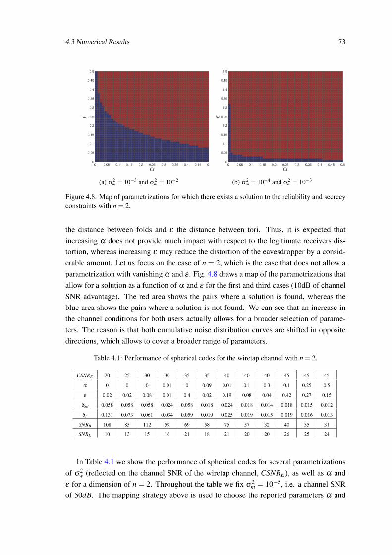
4.3 Numerical Results 73
(a) σ2m = 10−3 and σ2
m = 10−2 (b) σ2m = 10−4 and σ2
m = 10−3
Figure 4.8: Map of parametrizations for which there exists a solution to the reliability and secrecyconstraints with n = 2.
the distance between folds and ε the distance between tori. Thus, it is expected thatincreasing α does not provide much impact with respect to the legitimate receivers dis-tortion, whereas increasing ε may reduce the distortion of the eavesdropper by a consid-erable amount. Let us focus on the case of n = 2, which is the case that does not allow aparametrization with vanishing α and ε . Fig. 4.8 draws a map of the parametrizations thatallow for a solution as a function of α and ε for the first and third cases (10dB of channelSNR advantage). The red area shows the pairs where a solution is found, whereas theblue area shows the pairs where a solution is not found. We can see that an increase inthe channel conditions for both users actually allows for a broader selection of parame-ters. The reason is that both cumulative noise distribution curves are shifted in oppositedirections, which allows to cover a broader range of parameters.
Table 4.1: Performance of spherical codes for the wiretap channel with n = 2.
CSNRE 20 25 30 30 35 35 40 40 40 45 45 45
α 0 0 0 0.01 0 0.09 0.01 0.1 0.3 0.1 0.25 0.5
ε 0.02 0.02 0.08 0.01 0.4 0.02 0.19 0.08 0.04 0.42 0.27 0.15
δSB 0.058 0.058 0.058 0.024 0.058 0.018 0.024 0.018 0.014 0.018 0.015 0.012
δT 0.131 0.073 0.061 0.034 0.059 0.019 0.025 0.019 0.015 0.019 0.016 0.013
SNRB 108 85 112 59 69 58 75 57 32 40 35 31
SNRE 10 13 15 16 21 18 21 20 20 26 25 24
In Table 4.1 we show the performance of spherical codes for several parametrizationsof σ2
w (reflected on the channel SNR of the wiretap channel, CSNRE), as well as α andε for a dimension of n = 2. Throughout the table we fix σ2
m = 10−5, i.e. a channel SNRof 50dB. The mapping strategy above is used to choose the reported parameters α and

74 Continuous Spherical Codes for Secrecy
ε . For smaller value of CSNRE we see that both α and ε may take small values. On theother hand, for values of CSNRE closer to the main channel CSNR, a relaxation of ε (orα) is required. It is interesting to see how the distances δSB and δT vary according tothese parameters. While for the cases of lower CSNRE it is possible to obtain distancesδSB and δT that are already some distance apart, the same is not true with respect to thecases where CSNRE increases. The reason is that for such values of wiretap CSNR, thecumulative curves have a very sharp decay. Moreover, as CSNRE approximates the mainchannel CSNR, the cumulative noise distributions become almost complementary curves.Thus, in such cases one must increase the code’s dimensions in order to be able to exploitthe distance diversity. Fig. 4.9 illustrates this point. Here we fix the main channel CSNRat 50dB and the wiretap channel CSNR at 45dB and let the dimension increase. As it in-creases, we see that the cumulative noise distributions have a less sharp decay. Moreover,the difference between channels becomes more noticeable, as the cumulative distributionsare longer complements of each other. Under such conditions it is now possible to use α
and β to provide for trade-offs that have the desired consequence of ensuring that δSB andδT are sufficiently far apart. Table 4.1 also shows that the eavesdropper’s output SNR,although increasing with the wiretap channel SNR, is constantly kept small. We note thatthere are two effects under play. When δSB and δT are not similar, the eavesdropper’sdistortion is mostly affected by torus errors. However, when both are similar, there is alsoa large distortion contribution from fold errors. This can be seen in the largest values ofCSNRE , where we allow a larger value of ε , but still the eavesdropper as a low outputSNR. From the legitimate receiver’s perspective, we see that when δSB and δT are closer,the distortion is greatly impacted. While the fraction of torus errors for the legitimatereceivers is residual, the fact that the considered values for δSB are very small impactsnegatively on its distortion, especially in such low dimensions.
4.4 Discussion
We have proposed the use of spherical codes based on flat tori as the foundation of acoding scheme for the Gaussian wiretap channel with continuous inputs. The scheme in-herits the advantages of spherical codes: efficient encoding/decoding, good performancein the high SNR regime and bandwidth expansion. We show that a careful parametrizationof these codes (which takes into account their geometrical properties) enables legitimateusers to communicate under a small distortion, while forcing the eavesdropper to operateat larger distortions. Moreover, the proposed construction provides a simple mechanismto trade-off reliability with secrecy.
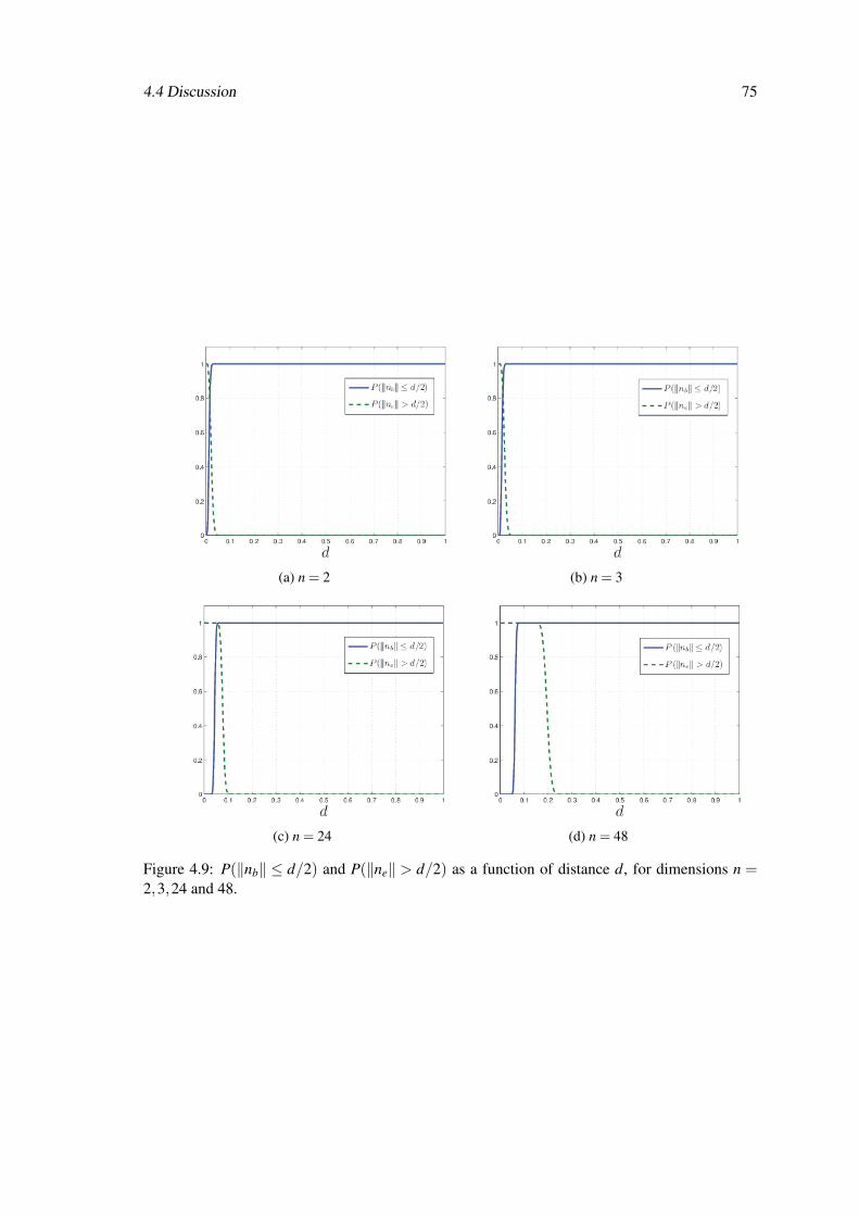
4.4 Discussion 75
(a) n = 2 (b) n = 3
(c) n = 24 (d) n = 48
Figure 4.9: P(‖nb‖ ≤ d/2) and P(‖ne‖ > d/2) as a function of distance d, for dimensions n =2,3,24 and 48.

76 Continuous Spherical Codes for Secrecy

Chapter 5
Randomly Punctured LDPC Codes forSecrecy
Rate-compatible coding [57, 58, 59] is an error-control strategy that allows to adapt therate of a given code to the channel statistics. The design principle behind these codes isto use a low-rate code whenever channel conditions are not favourable and a high-ratecode embedded in the low-rate code whenever channel conditions improve. Hence, rate-compatible codes use the same underlying structure regardless of channel conditions.
One of the most efficient ways of implementing rate compatible codes is throughpuncturing. This technique consists in selecting only a subset of the encoded bits fromthe original codewords for transmission. The bits that are not selected are said to be punc-tured. Typically, the puncturing operation is deterministic in the sense that puncturingpatterns are agreed upon a priori for the desired rates. However, the puncturing operationcan also be stochastic, i.e. bits can be randomly punctured. The latter approach however,requires some sort of mechanism to inform the receiver of the positions of punctured bits.
In the context of physical-layer security, the first secrecy strategy that used puncturingwas developed in the context of the Gaussian wiretap channel [19]. The authors showedthat, under belief propagation decoding, the eavesdropper will experience bit error rates(BER) close to 0.5 if its signal to noise ratio is lower than a given threshold. Consequently,the eavesdropper’s observations contained nearly i.i.d errors, and non-decodability couldbe ensured. With respect to secrecy metrics, [19] introduces a new secrecy metric calledthe security gap, which attempts at measuring the point at which decoding is successfulfor the legitimate receiver and fails for the eavesdropper. Then, puncturing distributionsare optimized in order to reduce the security gap. The idea is that, if the security gap canbe reduced to zero, then any stochastically degraded channel will be enough to ensurenon-decodability. Puncturing has also been used in the context of packet erasure channelswith authenticated feedback [60]. The availability of an authenticated feedback channelenables only the legitimate receiver to request retransmissions for missing packets, thus
77
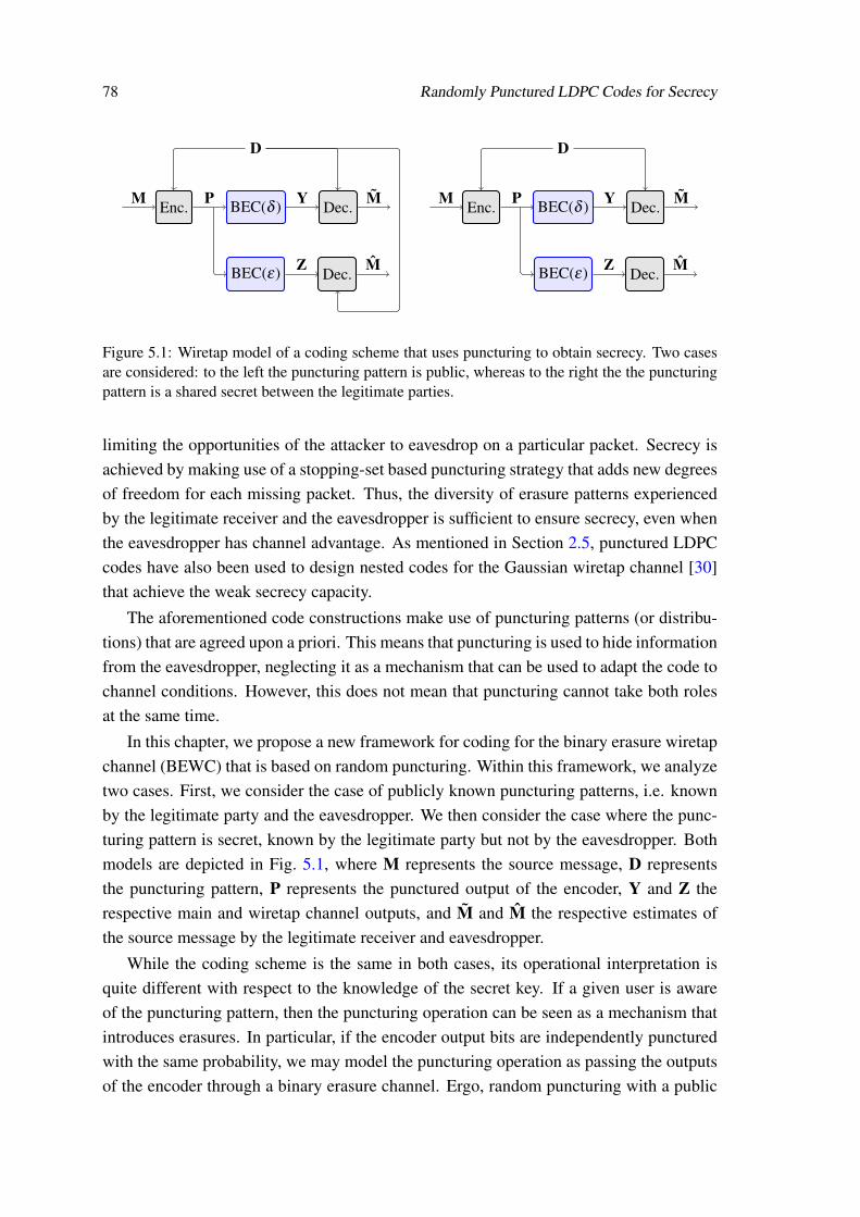
78 Randomly Punctured LDPC Codes for Secrecy
Enc. BEC(δ ) Dec.
BEC(ε) Dec.
D
M P Y M
Z M
Enc. BEC(δ ) Dec.
BEC(ε) Dec.
D
M P Y M
Z M
Figure 5.1: Wiretap model of a coding scheme that uses puncturing to obtain secrecy. Two casesare considered: to the left the puncturing pattern is public, whereas to the right the the puncturingpattern is a shared secret between the legitimate parties.
limiting the opportunities of the attacker to eavesdrop on a particular packet. Secrecy isachieved by making use of a stopping-set based puncturing strategy that adds new degreesof freedom for each missing packet. Thus, the diversity of erasure patterns experiencedby the legitimate receiver and the eavesdropper is sufficient to ensure secrecy, even whenthe eavesdropper has channel advantage. As mentioned in Section 2.5, punctured LDPCcodes have also been used to design nested codes for the Gaussian wiretap channel [30]that achieve the weak secrecy capacity.
The aforementioned code constructions make use of puncturing patterns (or distribu-tions) that are agreed upon a priori. This means that puncturing is used to hide informationfrom the eavesdropper, neglecting it as a mechanism that can be used to adapt the code tochannel conditions. However, this does not mean that puncturing cannot take both rolesat the same time.
In this chapter, we propose a new framework for coding for the binary erasure wiretapchannel (BEWC) that is based on random puncturing. Within this framework, we analyzetwo cases. First, we consider the case of publicly known puncturing patterns, i.e. knownby the legitimate party and the eavesdropper. We then consider the case where the punc-turing pattern is secret, known by the legitimate party but not by the eavesdropper. Bothmodels are depicted in Fig. 5.1, where M represents the source message, D representsthe puncturing pattern, P represents the punctured output of the encoder, Y and Z therespective main and wiretap channel outputs, and M and M the respective estimates ofthe source message by the legitimate receiver and eavesdropper.
While the coding scheme is the same in both cases, its operational interpretation isquite different with respect to the knowledge of the secret key. If a given user is awareof the puncturing pattern, then the puncturing operation can be seen as a mechanism thatintroduces erasures. In particular, if the encoder output bits are independently puncturedwith the same probability, we may model the puncturing operation as passing the outputsof the encoder through a binary erasure channel. Ergo, random puncturing with a public
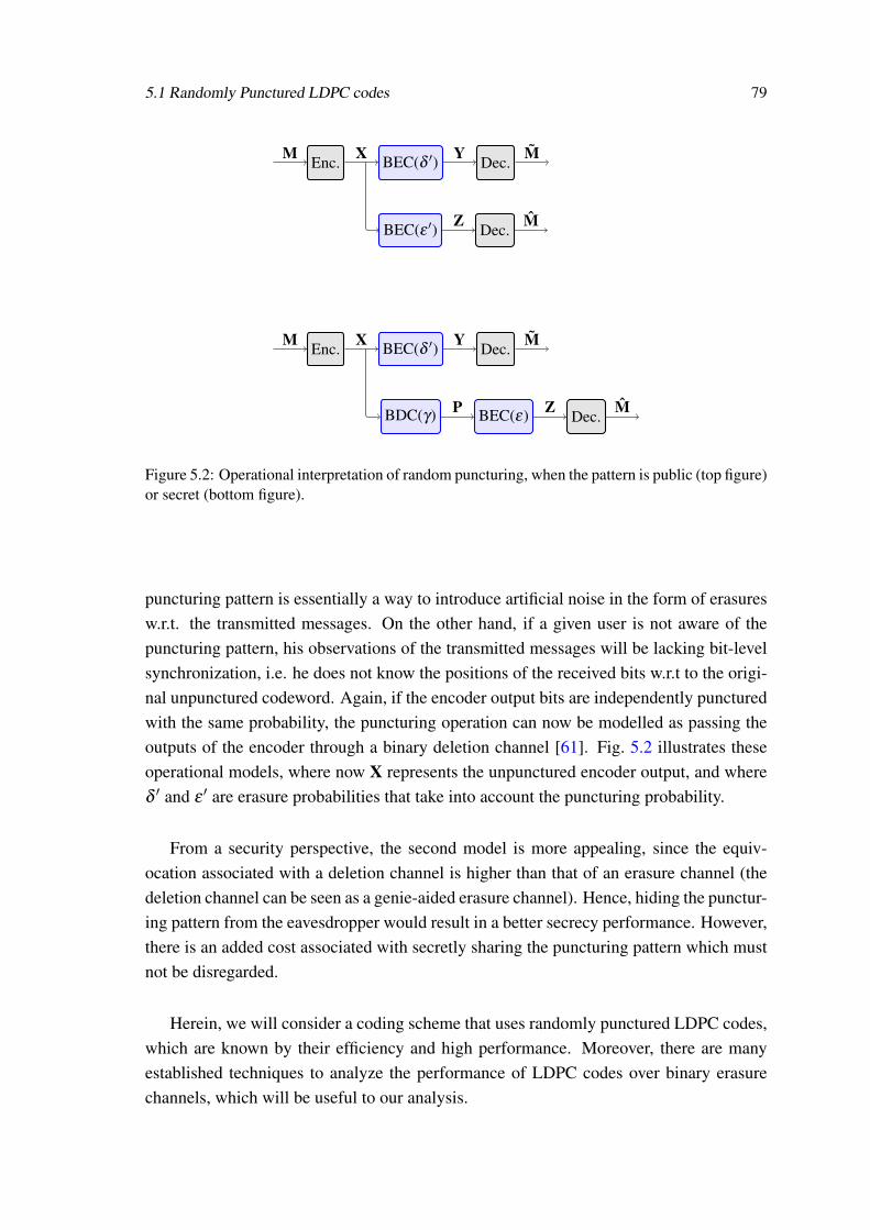
5.1 Randomly Punctured LDPC codes 79
Enc. BEC(δ ′) Dec.
BEC(ε ′) Dec.
M X Y M
Z M
Enc. BEC(δ ′) Dec.
BDC(γ) BEC(ε) Dec.
M X Y M
Z MP
Figure 5.2: Operational interpretation of random puncturing, when the pattern is public (top figure)or secret (bottom figure).
puncturing pattern is essentially a way to introduce artificial noise in the form of erasuresw.r.t. the transmitted messages. On the other hand, if a given user is not aware of thepuncturing pattern, his observations of the transmitted messages will be lacking bit-levelsynchronization, i.e. he does not know the positions of the received bits w.r.t to the origi-nal unpunctured codeword. Again, if the encoder output bits are independently puncturedwith the same probability, the puncturing operation can now be modelled as passing theoutputs of the encoder through a binary deletion channel [61]. Fig. 5.2 illustrates theseoperational models, where now X represents the unpunctured encoder output, and whereδ ′ and ε ′ are erasure probabilities that take into account the puncturing probability.
From a security perspective, the second model is more appealing, since the equiv-ocation associated with a deletion channel is higher than that of an erasure channel (thedeletion channel can be seen as a genie-aided erasure channel). Hence, hiding the punctur-ing pattern from the eavesdropper would result in a better secrecy performance. However,there is an added cost associated with secretly sharing the puncturing pattern which mustnot be disregarded.
Herein, we will consider a coding scheme that uses randomly punctured LDPC codes,which are known by their efficiency and high performance. Moreover, there are manyestablished techniques to analyze the performance of LDPC codes over binary erasurechannels, which will be useful to our analysis.

80 Randomly Punctured LDPC Codes for Secrecy
v1
v2
v3
v4
v5
v6
v7
u1
u2
u3
Figure 5.3: Bipartite graph with n = 7 variable nodes (represented by circles) and n−k = 3 checknodes (represented by squares).
5.1 Randomly Punctured LDPC codes
An LDPC ensemble [62] of length n can be defined as an ensemble of bipartite graphscomprised of variable nodes and parity check nodes (illustrated in Fig 5.3). These bipar-tite graphs can be characterized by polynomial degree distributions [62] either from anedge perspective or from a node perspective. As usual, we will denote the variable nodeand parity check node degree distributions from an edge perspective by λ (x) and ρ(x),
respectively. In particular, we define λ (x) =c∑
l=2λlxl−1 and ρ(x) =
d∑
l=2ρlxl−1, where λl
and ρl represent the fraction of edges connected to variable nodes with degree l and thefraction of edges connected to parity check nodes with degree l and c and d represent themaximum degree of variable and check nodes. Then, we denote an LDPC ensemble asLDPC(n,λ ,ρ).
Similarly, we will denote the degree distributions from a node perspective by Λ(x)
(variable node) and Γ(x) (parity check node). We define Λ(x) =c∑
l=2Λlxl and Γ(x) =
d∑
l=2Γlxl , where Λl and Γl represent, respectively, the fraction of variable nodes with degree
l and the fraction of parity check nodes with degree l and c and d are defined as above.The conversion between the degree distributions from the edge perspective to the nodeperspective (and vice-versa) are given by the following two relations:
λ (x) =Λ′(x)Λ′(1)
, ρ(x) =Γ′(x)Γ′(1)
.

5.1 Randomly Punctured LDPC codes 81
From the degree distributions it is possible to compute the design rate R of an LDPC code.
We have that R = 1− Γ
Λ, where Γ =
d∑
l=2
ρll and Λ =
c∑
l=2
λll .
A puncturing distribution for an LDPC code is similar to that of a code’s degree distri-
bution. We denote such distribution by γ(x) =c∑
l=2γlxl−1, where γl represents the fraction
of variable nodes of degree l that are punctured. The resulting punctured code has a de-
sign rate R∗ given by R∗ = R1−Λp
Λ
, where R is the initial code rate, Λp =c∑
l=2
γlλll , and Λ
is defined as before. As noted before, it is useful to think of the puncturing operation interms of an erasure channel. Therefore, we will specifically consider puncturing distribu-
tions of the form γ(x) =c∑
l=2γxl−1, i.e. each bit is punctured independently and uniformly
at random with probability γ .
5.1.1 Encoding and Decoding of LDPC Codes over Binary Erasure Channels
From an encoding and decoding perspective, LDPC codes are more useful when instancedas linear codes. An (n,k) linear binary block code is a set C ⊂ Fn
2 composed of 2k code-words of length n. The encoder is a bijective map between messages of k bits and code-words of n bits, while a decoder is a surjective map between the set of all binary sequencesof length n and the set C. Moreover, one of the code’s properties is that it is a subspaceof Fn
2 with dimension k. In particular, C is closed under addition, i.e. the sum of any twocodewords in C also belongs to C.
Encoding with linear block codes can be performed by multiplying m by a (k× n)generator matrix G, whose rows form a basis of the linear code, i.e. x=mG. It is possibleto associate with C an (n− k)×n parity check matrix H, with the property that xHᵀ = 0,for any x ∈ C. Then, for any sequence y ∈ Fn
2, it is possible to compute a quantity calledsyndrome which is given by s = yHᵀ. Thus, s = 0 if and only if y ∈ C. While decoding ofa binary linear code may take many forms, these are in general related to the parity checkmatrix. We will describe some possible decoding techniques latter in this section.
The connection between the definition of LDPC codes via degree distributions andvia a linear block code formulation is almost straightforward. Consider a code C ∈LDPC(n,λ ,ρ). LDPC(n,λ ,ρ) is a set of bipartite graphs that satisfy the constraints indi-cated by λ and ρ and C is a specific instance of such bipartite graph. Each of the bipartitegraphs in LDPC(n,λ ,ρ) can be represented (and fully defined) in terms of the paritycheck matrix H for specific values of k and n, where k is the length of the source messageand n is the desired codeword block-length n. The parity-check matrix H is an (n−k)×nmatrix, whose rows are associated with the check nodes of the bipartite graph and whosecolumns are associated with the variable nodes. Denote the set of variable nodes by de-noted V = (v1,v2, . . . ,vn), and the set of check nodes by denoted U = (u1,u2, . . . ,un−k).Then, Hi, j = 1 if and only if there is an edge between check node ui and variable node v j,

82 Randomly Punctured LDPC Codes for Secrecy
where Hi, j denotes the entry in H that corresponds to the i-th row and j-th column. Forthe bipartite graph in Fig. 5.3 we have the following parity check matrix.
H =
1 0 1 0 1 0 10 1 1 0 1 0 00 0 0 1 0 1 1
While the definition of an LDPC code is intrinsically connected to parity check ma-
trices, such connection is not obvious with respect to the generator matrix. However, wecan obtain the generator matrix from the parity check matrix as follows. Assuming thatH has full row rank, it is possible to use Gauss-Jordan elimination to put H into the formH = [A,In−k], from where we take G = [Ik,Aᵀ]1.
Decoding with LDPC codes can be performed using the general maximum a posteriori(MAP) block decoder obtained for linear block codes. If x∈C is the transmitted codewordand y is the received codeword and if codewords have a uniform prior distribution, thenthe MAP decoder is given by
x(y) = argmaxx
P(x|y). (5.1)
Now let E and E denote the set of indices of known bits and erased bits in y, respec-tively. Define the matrices HE and HE to be matrices including only the columns of Hindexed by E and E , respectively. Similarly, let xE and xE be vectors obtained from xthrough indexing of E and E . Since the received bits are either correct or erased, we canwrite 0 = Hxᵀ = HExᵀE +HExᵀE . In particular, since xE = yE , we simply need to solve forthe channel erased bits, i.e.
HExᵀE = sᵀ, (5.2)
where sᵀ = HExᵀE .
There may be more than one solution to (5.2) if it represents an under-determinedsystem of equations. However, it is possible to identify the set of compatible codewordsthat represent solutions to the above problem. Consider the following set XMAP(y) ={x ∈ C : sᵀ = HExᵀE}. Since all the elements in XMAP(y) are equally likely, we may definethe following rule for the MAP decoder (5.1)
x(y) =
x ∈ XMAP(y) , if |XMAP(y)|= 1
? , otherwise,
1It is also possible to use the parity check matrix for encoding [62, Appendix A] by putting H into an upper triangularform and considering codewords of the form x = (p,m), where m are the message bits and p are the parity bits, whichcan be found by back substitution from H.

5.1 Randomly Punctured LDPC codes 83
where ? denotes a decoding error. In particular, the MAP decoder provides a solutiononly when rank(HE) = |E|, i.e. the sub-matrix associated with the erased positions is fullrank2.
We have seen that MAP decoding can be accomplished by solving a system of linearequations. However, such strategy has a cubic polynomial complexity in general. Forefficiency reasons, LDPC decoding is generally accomplished using a belief-propagation(BP) decoder. The BP decoder [62] operates by passing messages (or beliefs) betweenvariable nodes and check nodes iteratively until errors are corrected (or a prescribed num-ber of iterations is reached). This process is summarized in algorithmic form in Algo-rithm 1, where sums are taken modulo 2. Note that BP decoders are sub-optimal withrespect to MAP decoders. The reason stems from the iterative nature of the algorithmthat can get stuck in the so called stopping sets, i.e. subsets of variable nodes such thatall neighbours of the subset are connected to it at least twice. In fact, after BP decodingtakes place, the remaining variable nodes containing erasures is the maximum stoppingset contained in the original set of erasures. In particular, for the possible erasure patterns,it is more frequent for a stopping set to occur than for the erasure pattern to be the sameas the support set of a codeword. Consequently, BP decoding fails in cases where MAPdecoding does not. Still, belief propagation decoders are known to approximate bit-wisemaximum a posteriori decoding and therefore, this decoding strategy generally achievesa good performance.
Algorithm 1 Belief propagation decoding over erasure channels.
1: Initialize: For y j 6=?, set each variable node v j = y j and send v j along the outgoing edges;2: if All variable nodes are known then3: Output the codeword.4: end if5: Processing at check nodes: At each check node ui, if there is an outgoing edge to variable
node v j, send a message to v j containing:6: 1) an erasure if there was some incoming message from vk, k 6= j that was an erasure;7: 2) a message containing the parity p = ∑
vk 6=v j
vk, where vk are the set variable nodes con-
nected to check node ui
8: Processing at variable nodes: At each variable node v j, if there is an incoming message fromcheck node ui that is not an erasure, set v j = ui and send v j along the outgoing edges;
9: if All variable nodes are known or no more progress can be made then10: Output the (possibly partial) codeword.11: else12: Go to Processing at check nodes (line 5).13: end if
While there are many possibilities for improving BP decoding over erasure channels,
2It is possible to further refine the estimate of the transmitted codeword by considering bit-wise map decoding,which leads to estimates of individual bits, rather than codewords.

84 Randomly Punctured LDPC Codes for Secrecy
there is a conceptual decoder that is useful for characterizing the difference in terms ofperformance of BP and MAP decoding. Consider the following variation of the BP de-scribed earlier. In the check node processing stage accumulate the values of the incomingmessages and delete all the edges that stem from variable nodes whose bit is alreadyknown. Then randomly select a check node of degree 1 and send its accumulate valuesonto the remaining outgoing edge. This determines the value of the respective variablenode that is connected to that check node. Now, select this variable node and transmitthe new found value along the remaining outgoing edges of this node and iteratively re-peat the procedure. When there are no more paths connecting either a variable node oran edge node, these can be discarded. At the end of the iterative procedure, a residualgraph will be obtained, containing the variable nodes that could not be resolved. If thisgraph is empty, decoding was successful. Otherwise, the remaining variable nodes forma maximum stopping set, just like in the previous case. This decoder is usually denotedas peeling decoder.
Let us illustrate this decoding process. Suppose that, using the LDPC code whosebipartite graph is depicted in Fig. 5.3, we transmit the codeword x = 1010111 and thechannel erases the second and fifth bits (see Fig. 5.4). In the first iteration, all non-erasedvariable nodes transmit their respective values along the outgoing edges. These values areaccumulated at the check nodes and the respective edges are erased. From the remaininggraph, it is possible to see that check node u1 has an induced degree of 1 and check node u2
has an induced degree of 2. Thus, we select check node u1 and transmit the accumulatedvalue along its outgoing edge, i.e. we send a message bit of 1 to variable node v5. Since wesend the value 1, the accumulated value on u1 is now 0. Furthermore, the edge connectingu1 and v5 can be removed. Upon setting v5 = 1, v5 sends its value along the remainingoutgoing edges, which at this point is only one edge to u2. The accumulated value at u2 isupdated to zero, the edge is erased, leaving u2 with an induced degree of 1. Therefore u2
can send its accumulated value to v2, determining the last erased bit. The residual graphin this case is empty, and the codeword was completely recovered.
Now consider the same code and transmitted codeword, where the channel erased bitsare now the third and fifth (depicted in Fig. 5.5). In this case, after setting the bit values ofthe variable nodes, sending them through the outgoing edges and removing these edges, itcan be seen that no check node as induced degree 1 (both u1 and u2 have induced degreeof 2). The peeling decoder thus gets stuck (it may output the partially decoded codeword)and the obtained residual graph is non-empty. In this case, it can be seen that v2 and v5
form a non-empty stopping set, and in particular, a MAP decoder cannot also decode thiscodeword, since the set of erasures includes a support set of the codeword (the sequences1000011 and 1010111 are valid codewords of the code). It should be noted that, in thelimit of an infinite number of iterations, both BP and peeling decoders have the sameperformance, as they get stuck in exactly the same structures.

5.1 Randomly Punctured LDPC codes 85
v1 = 1
v2 =?
v3 = 1
v4 = 0
v5 =?
v6 = 1
v7 = 1
u1
u2
u3
→
→→
→
→
→
→
1
?
1
0
?
1
1
1
1
0
←
1
?
1
0
1
1
1
0
1
0
→
1
?
1
0
1
1
1
0
0
0
←
1
0
1
0
1
1
1
0
0
0
Figure 5.4: Example of a peeling decoder that is able to recover the transmitted codeword.

86 Randomly Punctured LDPC Codes for Secrecy
v1 = 1
v2 = 0
v3 =?
v4 = 0
v5 =?
v6 = 1
v7 = 1
u1
u2
u3
→
→
→
→
→
→
1
0
?
0
?
1
1
0
0
0
Figure 5.5: Example of a peeling decoder that is not able to recover the transmitted codeword.
The connection between the performance of MAP decoders and BP decoders ariseswhen we consider a decoder known as Maxwell decoder. This decoder is a modificationof a peeling decoder in the following sense: whenever the peeling decoder gets stuck ina non-empty stopping set a symbolic variable, say si, is chosen to represent a value of acertain unresolved variable node vi. The decoder then proceeds as if this value is known.Thus, the messages passed are not only binary symbols but they may be equations. Atsome point, it is possible that such symbolic variable is connected to a check node of in-duced degree 1, which allows us to solve the symbolic variable si and therefore determinethe actual bit-value of the variable node vi. Moreover, we may possibly resolve otherequations that involve si. If all the introduced variables are resolved, we obtain the onlysolution that is compatible with the codeword. On the other hand, if some variables arenot resolved, we obtain a set of equations whose multiple solutions result in compatiblecodewords. Thus, the Maxwell decoder in fact performs MAP decoding by employinga peeling decoder with some sort of guessing device. Moreover, since it performs listdecoding, we may also relate the number of unresolved introduced variables to the con-ditional entropy of the code. These two aspects are what enable the performance analysisof MAP decoding and their connection to BP decoding.
5.1.2 LDPC Decoding Thresholds over Binary Erasure Channels
One way to assess the performance of LDPC codes is through the notion of decodingthresholds. Although the properties behind these thresholds are different in nature, theycapture the idea of characterizing the largest channel parameter that allows for reliablecommunication, given a certain code ensemble and decoding technique. In particular,

5.1 Randomly Punctured LDPC codes 87
they rely on concentration results, which essentially say that, for large enough block-lengths (n→ ∞) most matrices in an LDPC ensemble will exhibit the same properties.
For belief propagation decoding, the BP decoding threshold εBP is defined as thelargest channel erasure probability such that the bit erasure probability goes to zero asthe block-length and the number of decoding iterations goes to infinity. Formally, the BPdecoding threshold can be defined as follows:
limt→∞
Pb(n,ε, t) = 0, if ε < εBP (5.3)
and
limt→∞
Pb(n,ε, t)> 0, if ε > εBP. (5.4)
Here, Pb is the bit erasure probability, n is the code block-length, t is the number ofdecoding iterations and ε is the channel erasure probability.
For a given LDPC ensemble characterized by the polynomial degree distributions λ (x)and ρ(x), it is possible to obtain and analyze the BP decoding threshold with densityevolution techniques [62, 63]. Density evolution techniques track the evolution of theprobability density functions associated with the messages passing from check nodes tovariable nodes and vice-versa. For binary erasure channels, they track the probability thatthese messages are erasure messages. For non-punctured ensembles, the density evolutionequation F(x,ε) is given by [62]
F(x,ε) = x− ελ (1−ρ(1− x)). (5.5)
Thus, the decoding threshold εBP is the maximum value of ε ∈ [0,1], such that F(x,ε) =0 has no solution in x ∈ (0,1]. For punctured LDPC ensembles, the density evolutionequation is similar. Define the polynomials λp(x) and λ p(x) as
λp(x) =c
∑l=2
γlλlxl−1
and
λ p(x) =c
∑l=2
(1− γl)λlxl−1.
Then, the density evolution equation is given by [63]
Fp(x,ε) = x−λp(1−ρ(1− x))− ελ p(1−ρ(1− x)). (5.6)
Consequently, the decoding threshold for puncture codes εBPp is the maximum value of
ε ∈ [0,1], such that Fp(x,ε) = 0 has no solution in x ∈ (0,1].

88 Randomly Punctured LDPC Codes for Secrecy
For maximum a posteriori decoding, the MAP decoding threshold εMAP is defined hasthe largest erasure probability such that the normalized conditional entropy of the codeconverges to zero [64]. The general method for computing the MAP threshold of a certainensemble uses the EXIT curves of a BP decoder. The idea is as follows. Given the BPEXIT curve take a vertical line starting at εBP
p and shift it to the right. When the area underthe BP curve to the left of the line is equal to the area under the BP curve to the right ofthe line, the abscissa of this line marks the MAP threshold, giving rise to a generalizedarea theorem for erasure channels [64].
While determining the MAP threshold may be complicated for many ensembles (BPEXIT curves may have many discontinuities, for certain ensembles it is possible to obtaina straightforward computation of the MAP threshold using the notion of a peeling de-coder. It can be shown that the residual graph obtained by a peeling decoder is uniformlydistributed conditioned on its degree profile [65] and that its degree distribution pair issharply concentrated around its expected value [64]. More precisely, consider an LDPCensemble (n, λ , ρ) which is used for transmission over a BEC(ε). A peeling decodergives rise (w.h.p) to a residual ensemble (Λε , Γε ) with the following distribution [64]
Λε(z) , εΛ(zy) (5.7)
Γε(z) , Γ(x+ zx)−Γ(x)− zxΓ′(x), (5.8)
where x is the fixed point of the density evolution equation of the BP decoder, x , 1− xand y , 1−ρ(1− x).
The normalized equivocation is then given by the average rate of the residual ensem-ble [64]. Moreover, if the design rate of the residual ensemble is equal to its average rate,the normalized equivocation can be computed from this quantity. The following concen-tration lemma [64] provides us a way to identify which ensembles satisfy such constraint.
Lemma 4 ([64], Lemma 7). Consider an LDPC ensemble (n,λ ,ρ) with a design rater , 1− Λ′(1)
Γ′(1) . Let φ(x) = log2(1+ x) and consider the function Ψ(u) defined as
Ψ(u) =−Λ′(1)[φ(uv)−φ(v)]+∑
lΛlφ(ul)+(1− r)∑
lΓlφ
((1− v1+ v
)l)−Λ(1),
where v =(
∑l
λl1+ul
)−1(∑l
λlul−1
1+ul
).
Let G be a code picked uniformly at random from the ensemble LDPC(n,λ ,ρ) with arate rG. If Ψ(u) takes on its global maximum at u = 1, for u ∈ [0,∞), then there existsB > 0 such that, for any ξ > 0 and n > n0(ξ ,Λ,Γ),
Pr{|rG− r|> ξ} ≤ e−Bnξ .

5.1 Randomly Punctured LDPC codes 89
Thus, if the condition from Lemma 4 on Ψ(u) is met for the ensemble LDPC(n,λ ,ρ),with high probability, the design rate of the code will be asymptotically close to the aver-age code rate.
The following theorem provides the basis to compute the average normalized equivo-cation for a randomly chosen code for an ensemble LDPC(n,λ ,ρ).
Theorem 5 ([64], Theorem 10). Consider the LDPC ensemble (n,λ ,ρ). Let G be a codepicked at random from this ensemble, (Λε ,Γε ) be the corresponding residual ensemblewith respect to the transmission over a BEC(ε) and let the conditions of Lemma 4 holdfor the residual ensemble. Then,
limn→∞
1nE[HG(X|Z)]=Λ
′(1)x(1− y)− Λ′(1)Γ′(1)
[1−Γ(1− x)]+ εΛ(y),
where Λ and Γ are the degree distributions of the ensemble from a node perspective, x isthe fixed point of the density evolution equation of the BP decoder and y , 1−ρ(1− x).
Since by definition the MAP threshold is the largest channel erasure probability suchthat the normalized conditional entropy of the code converges to zero, Theorem 5 can beused to numerically find the code’s MAP threshold.
5.1.3 LDPC Decoding over Binary Deletion Channels with Erasures
As noted in the beginning of this chapter, if the puncturing pattern is not known to theeavesdropper, the observations of the eavesdropper can be described as the outputs of adeletion channel concatenated with a binary erasure channel (recall that we are consider-ing a binary erasure wiretap channel model). Therefore, it is useful to derive the MAPdecoder associated for the eavesdropper’s estimates under this setting. This MAP decodercan be described as follows.
Let x ∈ X be a randomly chosen codeword to be transmitted from a uniformly dis-tributed source. Let also p ∈ P be the resulting sequence from puncturing x using thepuncturing pattern d = (d1, . . . ,dn) ∈ D and z ∈ Z be the sequence that results from eras-ing the bits from p using the erasure pattern e = (e1, . . . ,en−nd) ∈ E, where nd = ∑
ni=1 di.
Assuming that bits are punctured and erased uniformly, we can derive the conditionalprobability P(p|x) as follows:
P(p|x) = ∑d
P(p|x,d)P(d|x)
= ∑d
P(p|x,d)P(d).

90 Randomly Punctured LDPC Codes for Secrecy
We know that
P(p|x,d) =
1, if ΠD(x,d) = p
0, otherwise,
with ΠD(x,d) denoting the sequence obtained by puncturing x with the pattern d. Thus,summing over d, we can group all the puncturing patterns that originate the same p.Noting that |p|= n−nd , we can write
P(p|x) = f (p,x)(1− γ)|p|γ |x|−|p|, (5.9)
where f (p,x) denotes the number of times p appears as a subsequence of x. In particular,since the generation of p by puncturing of x implies patterns that always have the sameweight, we have that P(d) = (1− γ)|p|γ |x|−|p| and (5.9) follows. Then, using the fact that(X,D)→ (P,E)→ Z forms a Markov chain, we can write
P(z|x) = ∑p
P(z|p)P(p|x)
= ∑p
P(z|p) f (p,x)(1− γ)|p|γ |x|−|p|
Now note that for a given p, any erasure pattern generates a different sequence z with thesame size as p. Hence, we have that
P(z|x) = ∑p:|p|=|z|
f (p,x)(1−γ)|p|γ |x|−|p|(1−ε)|p|−neεne , (5.10)
where ne is the number of erasures in z. Thus, P(z|x) can be found by computing thenumber of ways a subsequence p can be generated from x and summing over all thesubsequences that are compatible with z through erasures.
Now, let x be a randomly chosen codeword to be transmitted from a uniformly dis-tributed source and let z be the sequence observed by the eavesdropper after puncturingand channel erasures. The MAP estimate x of x is given by
x = argmaxx
P(x|z)
= argmaxx
P(z|x)P(x)P(z)
= argmaxx
P(z|x),
where P(z|x) can be computed from (5.10). signifies There are a couple of aspects toretain from the above derivation. First, the conditional probability P(z|x) depends onthe number of times an erased subsequence z is compatible with a given codeword x.Unfortunately, there are no known bounds on such distribution for arbitrary lengths of x.

5.2 Puncturing for Secrecy over the BEWC 91
Thus, in principle, these have to be computed on a code basis. Hence, for the case of secretpuncturing patterns, we may use a very efficient decoder at the legitimate receiver (e.g.BP decoding), while the eavesdropper’s optimal decoder will be very inefficient (countingthe number of sub-sequences can be solved with polynomial complexity [66]; howeverthis problem must be solved for every possible codeword). On the other hand, since thecomputation of equivocation of the eavesdropper requires this conditional probability, thesame problem will be present. Consequently, an exact equivocation analysis can only bedone for small block-lengths.
5.2 Puncturing for Secrecy over the BEWC
Consider the wiretap models depicted Fig. 5.2. The transmitter (Alice) wishes to send amessage M ∈ {0,1}k to the legitimate receiver (Bob), while preventing an eavesdrop-per (Eve) from obtaining a correct copy of that message. To achieve this, Alice en-codes M into the codeword X ∈ {0,1}n using a code from an ensemble LDPC(n,λ ,ρ).The outputs of the LDPC encoder are further punctured according to the distributionγ(x) = ∑
cl=2 γxl−1, where γ represents the probability of a variable node being punctured
(irrespective of its degree). Let D be a random variable that represents the puncturingpattern, such that D ∈ {0,1}n, where a 0 in the i-th entry of vector D means that the i-th message bit remains unpunctured, whereas a 1 determines that the i-th message bit ispunctured. Then, the channel input P is given by taking the values of X that are indexedby 0-entries in D. Upon transmission of the punctured message, Bob and Eve observe(noisy) copies of P, respectively through the main channel Qm and the wiretap channelQw. Both channels are assumed to be binary erasure channels with erasure probabilitiesδ for Qm and ε for Qw. Bob receives Y ∈ {0,1,?}n−nd , where ”?” represents an erasureand nd is the number of punctured bits, and makes an estimate M of the source message.Eve obtains Z ∈ {0,1,?}n−nd , which she also uses to make an estimate M of the sourcemessage.
By definition, this coding scheme is deterministic (and bijective). We are interested inunderstanding how using this simple encoding procedure can be enough to ensure reliableand secure communication and compare it with a more sophisticated approach, such asusing nested codes. In this context, we say that reliable communication is possible if theprobability of error is vanishing. On the other hand, we will measure secrecy throughthe code’s equivocation. Note that we do not set (a priori) a particular secrecy constraint.The reason is that we are interested in measuring the secrecy associated with the codingscheme, rather than setting up an initial goal such as achieving weak secrecy capacity.That being said, our objective is to maximize the equivocation experienced by the eaves-dropper (similar to a best effort approach to secrecy).

92 Randomly Punctured LDPC Codes for Secrecy
With respect to the nature of the puncturing pattern (public or secret), there is a clearimpact in terms of the secrecy analysis, as it is affected by the side information possessedby the eavesdropper. On the other hand, the reliability analysis is essentially the same,since in both cases the puncturing pattern is known by the legitimate party.
5.2.1 Reliability
The coding scheme under consideration has a single parameter that can be adjusted,namely the puncturing probability. It is possible to obtain very simple bounds on themaximum puncturing probability, for a given code ensemble, such that it allows vanish-ing error probability is obtained. Moreover, for the case of LDPC codes, it is also possibleto connect this puncturing probability to the type of decoder one wishes to use at the le-gitimate receiver through the decoding thresholds.
In general, let ε∗ denote the decoding threshold associated with an ensemble LDPC(n,λ ,ρ).Thus, with high probability, lim
n→∞Pe(Cn) = 0, if δ < ε∗, where Cn is an instance of the
LDPC ensemble.When modelling random puncturing as an erasure channel, our coding scheme can
be seen as using the original LDPC ensemble to transmit over a binary erasure channelcharaterized by an erasure probability of δ ′ = γ +(1− γ)ε . Since reliable communica-tion is only possible if δ ′ < ε∗, we immediately obtain that the puncturing probability isbounded by
γ ≤ ε∗−δ
1−δ. (5.11)
In particular, for BP and MAP decoding, the thresholds can be computed accordingto the descriptions given in Section 5.1.2. Clearly, with increasing decoding thresholds,larger admissible puncturing probabilities are obtained. Thus, the choice of a particulardecoding strategy bears an impact in terms of secrecy, since higher puncturing proba-bilities imply a larger equivocation with respect to the eavesdropper. This introduces atrade-off between decoding complexity and secrecy, which may be useful when design-ing a particular system.
5.2.2 Secrecy
The secrecy performance of the proposed coding scheme will be measured in terms of theequivocation of the eavesdropper’s observations. For the considered model, it is given bythe following lemma.
Lemma 5. Let M, X, Z, D be random variables that represent respectively, the sourcemessage, the unpunctured encoded message, the eavesdropper’s observation and the

5.2 Puncturing for Secrecy over the BEWC 93
puncturing pattern. Then, H(M|Z) = H(M|X,Z)+H(X|Z,D)+H(D|Z)−H(D|X,Z)−H(X|M,Z).
Proof. The proof is obtained by multiple applications of the chain rule of entropy.
H(M|Z) = H(M,Z)−H(Z)
= H(M,X,Z)−H(X|M,Z)−H(Z)
= H(M|X,Z)+H(X,Z)−H(X|M,Z)−H(Z)
= H(M|X,Z)+H(X|Z)−H(X|M,Z)
= H(M|X,Z)+H(X,D|Z)−H(D|X,Z)−H(X|M,Z)
= H(M|X,Z)+H(X|Z,D)+H(D|Z)−H(D|X,Z)−H(X|M,Z)
= H(M|X,Z)+H(X|Z,D)+ I(X;D|Z)−H(X|M,Z)
The next two corollaries specify the eavesdropper’s equivocation to the case of a pub-lic or secret puncturing pattern using the proposed coding scheme, which consists ofdeterministic and bijective encoder.
Corollary 3. Let there be a one-to-one mapping between M and X (and vice-versa). If Dis publicly known, then H(M|Z) = H(X|Z,D).
Corollary 4. Let there be a one-to-one mapping between M and X (and vice-versa).If D is only known by the legitimate receiver, then H(M|Z) = H(X|Z,D) +H(D|Z)−H(D|X,Z).
Corollary 3 states that if the puncturing pattern is public, the eavesdropper’s equiv-ocation is the equivocation associated with the transmission of codewords over a binaryerasure channel with erasure probability γ + (1− γ)ε . On the other hand, Corollary 4states that hiding the puncture pattern from the eavesdropper results in added equivoca-tion since H(D|Z)−H(D|X,Z) = I(D;X|Z), which is always a non-negative quantity. Inparticular, this term is associated with the loss of bit-level synchronization at the eaves-dropper’s decoder. Both are a consequence of having H(M|X,Z)=H(X|M,Z)= 0, whilefor Corollary 3 it is further implied that H(D|Z) and H(D|X,Z) are zero, as D is known.
As noted before, computing the equivocation of certain ensemble can be done straight-forwardly, provided that the ensemble obeys certain criteria. On the other hand, comput-ing the equivocation of a code where D is unknown, requires the computation of condi-tional probabilities over that may take an exponential time to compute. This means that anexact analysis of the equivocation in this case can only be done for small block-lengths.Alternatively, it is possible to bound the equivocation of the eavesdropper by consideringthe connection between the MAP decoder error probability and the respective conditional
94 Randomly Punctured LDPC Codes for Secrecy
entropy. While the MAP decoder itself has exponential complexity, it may be reducedwith respect to the complexity of computing the equivocation. The reason is that theconditional probabilities to be computed in the MAP decoder only need to be computedover sequences of a certain length, meaning that a certain observation defines the weightof the puncturing patterns. This means that one compute the conditional probabilitieswith respect to these patterns, thus reducing the amount of computations that need to beperformed.
In [25], the authors provide expressions for bounding the equivocation using the MAPerror probability. Let Pe be the expected MAP error probability and consider the twofollowing functions Φ(Pe) and Φ∗(Pe) as given in [25]
Φ(Pe) = (1−Pe)i log2 i+h(iPe− (i−1)), (5.12)
and
Φ∗(Pe) = ai
(Pe−
i−1i
)+bi, (5.13)
with i−1i ≤ Pe ≤ i
i+1 , i = 1, . . . ,M−1 and where h(·) is the binary entropy function, M isthe alphabet size, ai = i(i+1) log2((i+1)/i) and bi = log2(i). Then, the equivocation ofthe eavesdropper is bounded according to the following:
Theorem 6 ([25], Theorem 1). Let Pe(X|Z) denote the MAP error probability and H(X|Z)denote the equivocation. Then,
Φ(Pe(X|Z))≥ H(X|Z)≥Φ∗(Pe(X|Z)) (5.14)
5.2.3 Rate-Equivocation Regions
While there are several ways in which the puncturing pattern can be shared among thelegitimate parties (discussed in more detail in Section 5.4), it is possible to do it purelyfrom an information-theoretic point of view. From this perspective, we need to derivethe rate-equivocation regions, as our wiretap model requires some side information. Thisside information can be provided either by an external source3 (genie-aided) or can begenerated and transmitted by the legitimate receiver. The disclosure strategy and natureof the puncturing pattern may define a variant of the wiretap model, which may result in amodified rate-equivocation region. For instance, if we assume that the puncturing patternis obtained via a genie, a model which considers a public puncturing pattern is simply the
3For instance using information-theoretic secret-key agreement schemes [3, Chapter 4].
5.2 Puncturing for Secrecy over the BEWC 95
wiretap model we have considered so far and introduced in Section 2.1. On the other hand,if the puncturing pattern is a shared secret we are dealing with a wiretap with a sharedkey [67]. In the case the puncturing pattern is to be transmitted, considering a puncturingpattern public can be equivalent to have a broadcast wiretap channel with common andconfidential messages (BCC) [14], where the common rate is the rate allocated to thetransmission of the puncturing pattern. This would be a worst case scenario, since inpractice we do not need to require that the eavesdropper decodes de puncturing pattern,and consequently the rate-equivocation region can be further extended. In the event thatwe assume that the puncturing pattern is to be transmitted and kept secret, we have againa simple wiretap channel where now the secret rate has to be split to account for themessages and patterns.
Table 5.1: Equivalence of rate-equivocation regions as a function of the disclosure strategy andnature of the puncturing pattern.
public D secret Dgenie-aided D WTC WTC-SKtransmitted D BCC WTC
In the following, we will consider that the puncturing pattern is obtained via a genie.Therefore, the two rate-equivocation regions of interest are the rate-equivocation regionsfor the wiretap channel and the wiretap channel with a shared key (a proof is provided inAppendix C).
Theorem 7. ([3, Corollary 3.3]) Consider a wiretap channel (X , Y , Z , pY Z|X(y,z|x)).For any joint distribution pUV X on U ×V ×X that factorizes as pU pV |U pX |V , the weakrate-equivocation region for this wiretap channel is the convex set
RWT =⋃
pUV X
RWT (pUV X), (5.15)
where
RWT (pUV X) =
(R,Re) :0≤ Re ≤ R≤ 1
n I(V n;Y n)
0≤ Re ≤ 1n
[I(V n;Y n|Un)− I(V n;Zn|Un)
] .
Theorem 8. Consider a wiretap channel (K, X , Y , Z , pY Z|X(y,z|x)), where K is the keyalphabet. Moreover, assume that the key has a fixed rate Rk. For any joint distributionpUV X on U×V×X that factorizes as pU pV |U pX |V , the weak rate-equivocation region for

96 Randomly Punctured LDPC Codes for Secrecy
this wiretap channel is the convex set
RSK =⋃
pUV X
RSK(pUV X), (5.16)
where
RSK(pUV X) =
(R,Re) :0≤ Re ≤ R≤ 1
n I(V n;Y n)
0≤ Re ≤ 1n
[I(V n;Y n|Un)− I(V n;Zn|Un)
]+Rk
.
For noisier wiretap channel models the above regions can be simplified by taking V n =
Xn and letting Un to be independent of (V n,Xn,Y n,Zn). It is not surprising that a sharedsecret extends the rate equivocation region (in the sense that the maximum equivocationof the eavesdropper saturates at a higher value), since the key-rate is given for free in thiscase. However, it is not clear whether there is an advantage in terms of simplifying thecoding process, since coding using a secret key may be an easier task than its keylesscounterpart. Note that secret-key agreement is generally considered to be easier thancoding for secrecy, and thus there is no added complexity in obtaining this model to starta priori.
5.3 Numerical Results
We have seen in Section 5.2.2 that the eavesdropper’s equivocation depends simply on thecode’s performance over the binary erasure channel when the puncturing pattern is public.When instead we consider a secret puncturing pattern, the eavesdropper’s equivocation isfurther affected by the shared information between the codewords and the puncturing pat-tern, given the eavesdropper’s observation. Given that this is the case, a simple strategyto increase the eavesdropper’s equivocation is to consider codes that allow for a largepuncturing probability, which corresponds to the creation of a wiretap channel with ahigh erasure probability. Note that the manageable puncturing probability is associatedwith the decoder being used. Let us first consider the secrecy performance of the pro-posed coding scheme with public puncturing patterns and then move to secret puncturingpatterns.
5.3.1 Asymptotic Performance with Public Puncturing Patterns
Consider the ensembles defined by the degree distribution pairs in Table 5.2, which iscomprised of three irregular codes. Note that all ensembles have small rates. This isdue to the fact that we wish to have a large puncturing probability and, therefore, enough

5.3 Numerical Results 97
redundancy must be added in order to account for reliability. The BP thresholds εBP andMAP thresholds εMAP are also listed in the same table. In particular, the BP thresholdsof codes C2 and C3 are very similar, while the MAP thresholds of C1 and C3 are also verysimilar.
Table 5.2: Degree distributions of LDPC code ensembles C1, C2 and C3.
C1 C2 C3
λ2 0.057143 - -
λ3 0.942857 0.06383 -
λ4 - 0.93617 0.067797
λ5 - - 0.932203
ρ3 0.085714 - -
ρ4 0.914286 - -
ρ5 - 0.106383 -
ρ6 - 0.893617 0.40678
ρ7 - - 0.59322
R 0.25 0.3333 0.25
εBP 0.6576 0.5129 0.5075
εMAP 0.7444 0.6654 0.7499
To understand how the puncturing probability affects the reliability limits of our code,we will first fix the main channel crossover probability δ . From (5.11), we may obtain thelargest admissible puncturing probability as a function of the decoding threshold. Fig. 5.6plots the largest puncturing probability γ∗ as a function of the main channel erasure proba-bility δ . There exists a symmetry between the admissible puncturing probabilities and thechannel parameter. Obviously, almost noiseless channels allow for very large puncturingprobabilities.
Having found the admissible puncturing probabilities, we may turn our attention to theequivocation rate experienced by the eavesdropper. In particular, the ensemble averageequivocation rate is given by Theorem 5 whenever the required conditions hold, (whichis the case for the considered codes) and can be computed through (5.9) for channelparameters above the MAP threshold (by definition the equivocation evaluates to zerobellow the MAP threshold).
Figures 5.7 and 5.8 plot the normalized equivocation, as a function of the eavesdrop-per’s channel erasure probability ε , for a noisy main channel with erasure probabilityδ = 0.25, for the respective puncturing probability γ∗. Fig. 5.7 illustrates that, punctur-ing up to the BP threshold limit, leads to a constant gap from the maximum achievableequivocation (solid black line) that is a function of the MAP threshold. Thus, if an LDPC

98 Randomly Punctured LDPC Codes for Secrecy
(a) Belief propagation decoding. (b) Maximum a posteriori decoding.
Figure 5.6: Maximum puncturing probability γ∗ as a function of the channel erasure probability δ
for the ensembles C1, C2 and C3 when using a BP and a MAP decoder.
code presents a reasonable gap between the BP and MAP thresholds, using puncturingwith a BP decoding scheme leads to non-negligible leakage to the eavesdropper. On theother hand, if the legitimate receiver is allowed to use a MAP decoder as in Fig. 5.8, theeavesdropper will have near maximum equivocation (the small gap is a function of thegap between the MAP threshold and the Shannon limit [62]). This is a consequence ofhaving artificially saturated the eavesdropper’s channel with erasures until decoding is nolonger possible.
It is interesting to see that, unlike nested codes that require the design of codes thatare capacity achieving for the eavesdroppers channel, puncturing can have a similar effectsimply by artificially creating a noisier channel to the eavesdropper. However, like nestedcodes, this requires the eavesdropper to have a channel that is worse than the main channelto allow for reliable communication and forces the legitimate receiver to use a maximum-likelihood decoder. Consequently, in order to obtain secure communication with randompublic puncturing patterns, these two constraints have to be taken into account.
Another interesting fact is that no care in the code design itself was needed, as long asthe puncturing probability approaches the limit imposed by the MAP threshold. Conse-quently, there is no need to know the statistics of the eavesdropper’s channel in order tomaximize its equivocation.
Finally, note that, due to the linearity of the equivocation, if the BP and MAP thresh-olds of a certain code are very close, the MAP decoder can be replaced by a BP decoderand obtain a similar secrecy performance, enabling more efficient decoding to take place.
Let us now consider how puncturing strategies can be placed within the rate-equivocationregion. For simplicity, let us assume that the channel is degraded and the input distribution
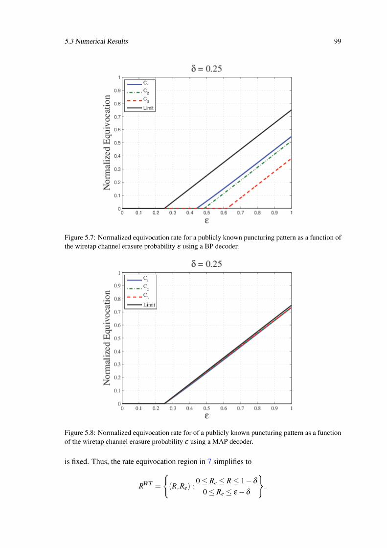
5.3 Numerical Results 99
Figure 5.7: Normalized equivocation rate for a publicly known puncturing pattern as a function ofthe wiretap channel erasure probability ε using a BP decoder.
Figure 5.8: Normalized equivocation rate for of a publicly known puncturing pattern as a functionof the wiretap channel erasure probability ε using a MAP decoder.
is fixed. Thus, the rate equivocation region in 7 simplifies to
RWT =
{(R,Re) :
0≤ Re ≤ R≤ 1−δ
0≤ Re ≤ ε−δ
}.

100 Randomly Punctured LDPC Codes for Secrecy
Fig. 5.9 illustrates, for the case of δ = 0.25, the rate-equivocation region (solid line)and the achievable rate-equivocation pairs for the considered ensembles (markers). Theachievable (R,Re) points are normalized to account for the puncturing probability, i.e., Ris the rate of the punctured code and Re is the equivocation normalized by the numberof unpunctured symbols. The plots shows that punctured LDPC codes, where the punc-turing probability is the largest admissible for a MAP decoder, operate near maximumequivocation at the eavesdropper. Naturally, the punctured code has also near maximumrate. Consequently, the code operates far from secrecy capacity. However, the code ratecan be artificially reduced by transmitting dummy bits. On the other hand, puncturing upto the BP threshold leads in general to considerable leakage rates. For instance, it can beseen that all codes provide no secrecy at all if ε = 0.30 (Fig. 5.9a), while little secrecy isprovided even when the channel advantage is large (Fig. 5.9b and Fig. 5.9b).
5.3.2 Finite-Length Performance with Secret Puncturing Patterns
While an asymptotic analysis is possible when the puncturing pattern is public (by virtueof being able to model the system using only erasure channels), when the puncturing pat-tern is secret, the assessment of the eavesdroppers equivocation is a cumbersome process,since it depends on the realization of the codebook (in particular of the sub-sequences ofcodewords).
In this section we sample the ensembles defined in Table 5.2 to obtain codes witha block-length n = 12. Since at such short block-lengths it is not possible to obtain avanishing error probability, we resort to the analysis of the exact code equivocation tofind the admissible puncturing probabilities. Fig. 5.10 provides a comparison betweenthe equivocation of the considered codes when n = 12 and for the asymptotic case. Asexpected, there is a large gap between the values of δ for which the legitimate receiver cancommunicate with near zero equivocation. Consequently, a reduction on the puncturingprobability is necessary. To allow for a reasonable puncturing probability, we allow thelegitimate receiver to incur in a small equivocation. This is represented in Fig. 5.10 by thedashed horizontal lines, where we mark the points at which the legitimate receiver makesestimates with an equivocation of a prescribed level.
Table 5.3: Puncturing probabilities of LDPC code ensembles C1, C2 and C3 with prescribed levelof equivocation.
C1 C2 C3
εBP 0.6576 0.5129 0.5075
εMAP 0.7444 0.6654 0.7499
γ1 0.3510 0.2645 0.3680
γ2 0.4965 0.4085 0.5150
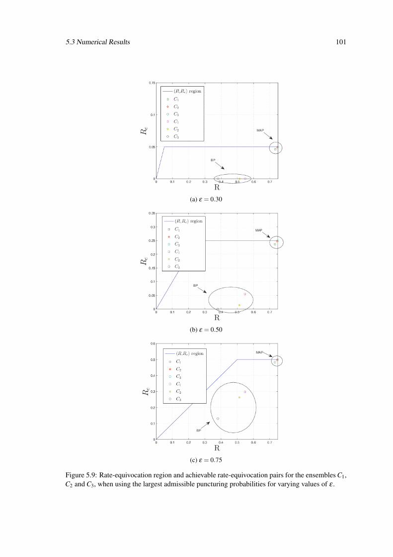
5.3 Numerical Results 101
(a) ε = 0.30
(b) ε = 0.50
(c) ε = 0.75
Figure 5.9: Rate-equivocation region and achievable rate-equivocation pairs for the ensembles C1,C2 and C3, when using the largest admissible puncturing probabilities for varying values of ε .
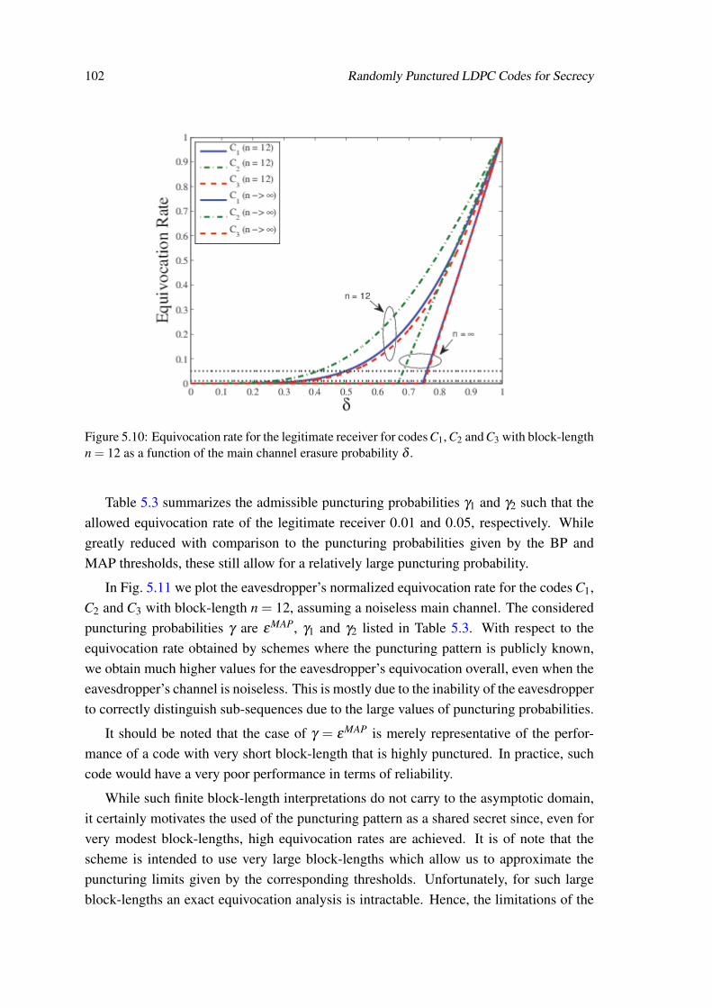
102 Randomly Punctured LDPC Codes for Secrecy
Figure 5.10: Equivocation rate for the legitimate receiver for codes C1, C2 and C3 with block-lengthn = 12 as a function of the main channel erasure probability δ .
Table 5.3 summarizes the admissible puncturing probabilities γ1 and γ2 such that theallowed equivocation rate of the legitimate receiver 0.01 and 0.05, respectively. Whilegreatly reduced with comparison to the puncturing probabilities given by the BP andMAP thresholds, these still allow for a relatively large puncturing probability.
In Fig. 5.11 we plot the eavesdropper’s normalized equivocation rate for the codes C1,C2 and C3 with block-length n = 12, assuming a noiseless main channel. The consideredpuncturing probabilities γ are εMAP, γ1 and γ2 listed in Table 5.3. With respect to theequivocation rate obtained by schemes where the puncturing pattern is publicly known,we obtain much higher values for the eavesdropper’s equivocation overall, even when theeavesdropper’s channel is noiseless. This is mostly due to the inability of the eavesdropperto correctly distinguish sub-sequences due to the large values of puncturing probabilities.
It should be noted that the case of γ = εMAP is merely representative of the perfor-mance of a code with very short block-length that is highly punctured. In practice, suchcode would have a very poor performance in terms of reliability.
While such finite block-length interpretations do not carry to the asymptotic domain,it certainly motivates the used of the puncturing pattern as a shared secret since, even forvery modest block-lengths, high equivocation rates are achieved. It is of note that thescheme is intended to use very large block-lengths which allow us to approximate thepuncturing limits given by the corresponding thresholds. Unfortunately, for such largeblock-lengths an exact equivocation analysis is intractable. Hence, the limitations of the

5.3 Numerical Results 103
Figure 5.11: Normalized equivocation rate for the eavesdropper for codes C1, C2 and C3 withblock-length n = 12, as a function of the wiretap channel erasure probability ε . The consideredpuncturing probabilities γ are equal to εMAP, γ1 and γ2.
analysis are due to fact that we cannot compute the eavesdropper’s equivocation ratherthan on establishing reliable communication.
Let us put the achievable rate-equivocation pairs in perspective. Consider the abovementioned ensembles C1, C2 and C3. Let the main channel be a noiseless channel and theeavesdropper’s channel have an erasure probability ε = 0.25. Let us further assume thatwe have a key of rate Rk ≥ 0.75 available, in the scenario where the puncturing patternsare secret.
Fig. 5.12 illustrates the rate-equivocation regions of both models, where the modelwithout a shared key is represented by a dashed blue line and the model with a sharedkey is represented by the solid black line. For the randomly drawn codes of block-lengthn = 12, consider a puncturing probability γ = γ1. It is possible to see that the achievableequivocation rates are already approaching the rate-equivocation region of the generalwiretap channel without a shared key (the three leftmost points of the plot). This shouldbe interpreted within the respective context, since we are allowing the legitimate receiverto have a small equivocation (as opposed to zero equivocation) and we have a shared keyof a large rate. Nevertheless, it is surprising that, for such small block-lengths, one canalmost reach the rate-equivocation region of the regular wiretap channel. For illustrativepurposes, we also plot the case where we have a block-length of n = 12 and punctureup to the MAP threshold (which implies a large equivocation on the legitimate receiverside). From the plot we can observe that puncturing up to the MAP thresholds pushes

104 Randomly Punctured LDPC Codes for Secrecy
the eavesdropper’s equivocation to near maximum equivocation. This suggests that forincreasing block-lengths, one can rapidly approach the secrecy capacity of this channelmodel. As a further comment, it should be noted that, even considering modest block-lengths, punctured codes with a secret puncturing pattern have a performance that is notvery far from its theoretical limit, considering the code construction in question is usingdeterministic and bijective encoders.
Figure 5.12: Rate-equivocation regions of the considered models and the rate-equivocation pairsfor codes C1, C2 and C3 for both the asymptotic and finite block-length case. Wiretap modelparameters are δ = 0 and ε = 0.25.
As noted before, it is possible to manage slightly larger block-lengths by focusing onthe eavesdroppers MAP decoder. To this purpose, we recur to simulation and computethe average MAP error probability, using Theorem 6 to bound the equivocation obtainedby the simulated average error probability. The employed codes have block-length n =
20 and their degree distribution are defined in Table 5.4, along with the BP threshold.The considered puncturing probability is bounded by the BP decoding threshold and thetransmission of 10000 codewords is considered. We considered both noiseless and noisymain channels, with the main channel erasure probabilities δ ∈ {0,0.1,0.25} and varyingwiretap channel erasure probabilities ε . Note that code C4 is a regular code, while codeC5 is an irregular code. Moreover, the puncturing probability is the maximum allowed byBP decoding.
Figs. 5.13 and 5.14 show the average bit error probability experienced by the eaves-dropper. For this particular case, it can be seen that the irregular code is able to constantlyachieve a high bit error rate, even when the channel to the eavesdropper is noiseless. On
5.4 System Aspects 105
Table 5.4: Degree distributions for the LDPC code ensembles C4, and C5.
C4 C5
λ2 - 0.25105λ3 1 0.30938λ4 - 0.00104λ10 - 0.43853ρ6 1 -ρ7 - 0.63676ρ8 - 0.36324
εBP 0.4294 0.4701
the other hand, the regular code performs well, but is more affected when the main chan-nel error probability increases, i.e. when the puncturing probability needs to be reduced.
The simulated equivocation bounds are plotted in Figs. 5.15 and 5.16, the regular andirregular code, respectively. In each figure, the dashed lines represent the lower bonds onthe equivocation obtained via simulation of the average error probability, while the solidlines represent the upper bounds. Each line color is associated with a particular erasureprobability of the main channel.
For a noiseless main channel, the bounds are tight. With increasing erasure proba-bilities over the main channel, the puncturing limit decreases, hence the eavesdropper’serror probability also decreases and the bounds become loose. For this particular case,even though the BP decoding thresholds are just slightly apart, the irregular code presentsmuch tighter bounds that the regular code.
In summary, it is possible to see that hiding the puncturing pattern results in a higherror rate, even when the eavesdropper’s estimates are optimal. Thus, even for modestblock-lengths, puncturing can provide secrecy benefits.
5.4 System Aspects
In this section we discuss several questions that pertain to the assumptions behind theproposed model as well as other system aspects.
5.4.1 Sharing Secret Keys
We have seen that using the puncturing pattern as a shared secret may help in increasingthe eavesdropper’s equivocation, due to the lack of synchronization. However, this re-quires either the transmission or agreement of a secret key. In practice this can be done inseveral ways. First, it is possible to use cryptographic methods such as the Diffie-Hellmankey agreement scheme [68]. Hence, a cross-layer approach may be taken in the systemdesign. Of course that the derived keys do not obey any information-theoretic secrecy

106 Randomly Punctured LDPC Codes for Secrecy
Figure 5.13: Simulated average bit error rate for the code C4 as a function of the wiretapchannel erasure probability ε , when the main channel erasure probability takes values fromδ ∈ {0,0.1,0.25}.
Figure 5.14: Simulated average bit error rate for the code C5 as a function of the wiretapchannel erasure probability ε , when the main channel erasure probability takes values fromδ ∈ {0,0.1,0.25}.

5.4 System Aspects 107
Figure 5.15: Bounds on the equivocation of simulated error probability for the code C4 as a func-tion of the wiretap channel erasure probability ε , when the main channel erasure probability takesvalues from δ ∈ {0,0.1,0.25}.
Figure 5.16: Bounds on the equivocation of simulated error probability for the code C5 as a func-tion of the wiretap channel erasure probability ε , when the main channel erasure probability takesvalues from δ ∈ {0,0.1,0.25}.

108 Randomly Punctured LDPC Codes for Secrecy
criterion, and therefore, the equivocation of the eavesdropper could in general be less, ashe may obtain some information about the puncturing pattern. Nevertheless, even in aworst case scenario where the eavesdropper obtains a perfect copy of the secret key, wehave seen that puncturing can provide for maximum equivocation (if we puncture up tothe MAP threshold). Thus, from a practical standpoint, using a cross-layer approach maybe sufficient for secrecy purposes.
On the other hand, one may use information-theoretic secret key agreement schemes [3,Chapters 3 and 4]. A possibility is to use a regular wiretap code to share this key. Whileapparently this would defeat the motivation for our scheme, this is not necessarily true, asthe wiretap code can be used in a conservative way (meaning that we use a wiretap codeassuming the quality of the wiretap channel that is very close to the quality of the mainchannel). Consequently, the secure rate would be small. However, if the code allows for alarge enough puncturing probability, the rate required for the secret key is also small, andtherefore such strategy may be sufficient. A second possibility that is more appealing isto use sequential key distillation strategies [3, Chapter 4.3], [69], either using one-way ortwo way communications. Unlike wiretap codes, sequential key distillation strategies donot require a better main channel, but they do require an external source. Lastly, it is alsopossible to use a parallel secure channel of limited rate, if such channel is available.
5.4.2 Secret Key Rates
The examples used in the previous section may suggest a large key rate is always requiredfor the scheme to be effective. Once again, this limitation is imposed in the examples dueto the fact that we may only compute the eavesdropper’s equivocation for small block-lengths. In fact, in the limit of large block-lengths, one expects to find codes of very lowrate and large MAP threshold, which would translate onto a reduced key rate. However,codes with very low rate require a very large block-length.
In particular, the proposed scheme requires Rk = Hb(εMAP), where Hb(·) is the binary
entropy function. Thus, for increasingly larger MAP thresholds (where reliability can beachieved by letting n→ ∞) we would need keys of very low rate. On the other hand, thepuncturing operation ensures that we actually communicate at an increased rate, thereforethe usage of such codes does not force us to operate with a low communication rate.
5.4.3 Comparison with the One-Time Pad Cryptosystem
Consider the system depicted in Fig. 5.17, where we have a BEWC and the encoderperforms one-time pad encryption. Assume that the messages are represented by an n-dimensional random variable M and chosen according to a i.i.d. uniform distribution.Let the employed key K be also an i.i.d. n-dimensional random variable that follows aBinomial distribution with probability γ . The transmitted message is given by X = M⊕

5.5 Discussion 109
Encoder Decoder
BEC(ε)
K
M X M
Z
Figure 5.17: Shannon Cipher System with erasures.
K, where ⊕ represents the modulo 2 addition operation. The normalized equivocation1nH(M|Z) can be upper bounded as follows:
1n
H(Mn|Zn) =1n
H(Mn,Kn|Zn)− 1n
H(Kn|Mn,Zn)
=1n
H(Kn|Zn)+1n
H(Mn|Kn,Zn)− 1n
H(Kn|Mn,Zn)
≤ 1n
H(Kn)+1n
H(Mn|Kn,Zn)− 1n
H(Kn|Mn,Zn)
= (1− ε)H(K)+ εH(M).
Since we have assumed a uniform input distribution, this expression simplifies to1nH(Mn|Zn) = H(K)+ ε(1−H(K)). Obviously, if the wiretap channel is noiseless (ε =
0), the eavesdropper’s equivocation will amount to the key equivocation. Thus, if we haveaccess to a truly random key we will be able to operate at secrecy capacity with a one-timepad. However, if we only have access to a very biased key, the eavesdropper’s equivo-cation will decrease. The same relationship is not true in our scheme. A biased key (oflower rate) will lead to an increase in equivocation, since more bits can be punctured (pro-vided that we satisfy the reliability constraint). Moreover, if by some reason an adversaryobtains the key used in the system, the eavesdropper’s equivocation will amount to theerasure probability of the wiretap channel when the one-time pad scheme is used, whilein the proposed scheme the eavesdropper’s equivocation will amount the modified chan-nel erasure probability, which is always larger than the original wiretap channel erasureprobability.
5.5 Discussion
In this chapter we have proposed the use of random puncturing for secrecy over the erasurewiretap channel. We have shown that, to achieve high equivocation rates using a publicpuncturing pattern and a bijective deterministic encoder, the legitimate user is requiredto use a MAP decoder and puncture bits with a probability up to the MAP threshold. If

110 Randomly Punctured LDPC Codes for Secrecy
the puncturing pattern is used as a shared secret, higher secrecy rates can be achieved. Ifthe secret key is derived using physical-layer security methods, then the equivocation rateanalysis has to take this fact into account. However, this shared secret can also be derivedby public key cryptographic schemes, providing a cross-layer solution to the problem ofconfidential data transmission. Among the benefits provided by random puncturing is aneasy adaptation of the code rate to the main channel, as well as avoidance of the need forchannel statistics of the eavesdropper. It also provides easy guidelines for code design, asthe only requirement is to puncture up to the permitted thresholds. An interesting point isalso worth noting. The use of a puncturing pattern as a shared secret essentially creates awiretap channel model that is fundamentally different from the main channel. This differ-ence implies that the optimal source distribution with respect to the main channel (whichis the one used in practice), may not be optimal for the wiretap channel (for instance, theuniform distribution is not the optimal input distribution for the deletion [61]). This canbe seen as a further advantage in using such schemes.

Chapter 6
Conclusions
Under the paradigm of physical-layer security, we develop several coding schemes toprovide for confidential data transmission. The focus is essentially mostly on practicalcode constructions. Our work differs from other works in this field in several ways. First,we explicitly design codes for finite block-lengths, which contrasts with the traditionalasymptotic code designs. Second, we provide code constructions for continuous sources.Hence, our work does not inherit the assumptions required for separation theorems tohold. Third, we consider deterministic code constructions, thus circumventing the needfor wiretap channel state information, as well as the need to optimize the use of localrandomness. These differences also translate onto several limitations that can be assignedto our code constructions. The greatest perhaps is that, in general, our coding schemesdo not achieve the fundamental limits of secrecy. On the other hand, their performancedepends on the chosen block-length. In particular, for very small block-lengths, we haveshown a relaxation is generally required, with respect to the reliability and secrecy criteria.
In summary, our main contributions can be stated as follows. In Chapters 3 and 4we addressed code designs for continuous sources. In the former, a joint-source channelcode is proposed which hinders the eavesdropper by forcing him to operate at a desireddistortion level. This is accomplished by solving an optimization problem over the codeparameters which constitutes in finding the scalar quantizer boundaries as well as the cor-responding channel code that satisfies the aforementioned secrecy constraint. In the latterchapter, we use a particular instance of bandwidth expansion mappings which allows usto enforce anomalous errors for the eavesdropper, resulting in a large distortion. In partic-ular, the code is parametrized based on its geometrical properties to ensure this constraintis satisfied. As a further advantage, these codes allow for very efficient encoding anddecoding schemes. Chapter 5 proposes the use of random puncturing in order to create awiretap channel of very poor quality to the eavesdropper, ensuring that his equivocationis highly increased. Using the insight that the loss of bit-level synchronization generallycreates a channel with reduced capacity, we propose the use of the puncturing pattern as
111
112 Conclusions
a shared secret, showing that, in such scenarios, the eavesdropper is bound to have a highequivocation, even for very small block-lengths.
6.1 Future Research
The coding schemes and the general framework under which these schemes are treatedcan be extended in multiple ways.
• Nested Code Constructions: While we avoid the use of nested code constructionsto circumvent the issues of the lack of wiretap channel state information, this is notnecessarily true in all cases. Therefore, there it could be interesting to extend thesecode constructions to use nested structures. While this has been largely done inthe context of codes for discrete sources (see e.g.Chapter 2), the design of contin-ues nested codes is practically non-existent. For instance, the code construction inChapter 3 can be extended to the use of multiple scalar quantizers, each one withnon-overlapping channel codes and optimized boundaries. The code constructionin Chapter 4 could be extended to account for a multiple correspondence betweensource intervals and tori or source intervals and parallel curves over a given torus.
• Secrecy from the absence of synchronization: In Chapter 5 we have studied thesecrecy performance of LDPC codes when the puncturing pattern was a shared se-cret. Consequently, this strategy induced a wiretap channel with deletions. Littleis known with respect to the deletion channel. Thus, advances in the understand-ing of this channel model could benefit a more fundamental understanding of theperformance of the secrecy codes proposed here. In particular, it could interestingto understand if it is possible to induce a deletion channel of zero capacity usingthis channel model, which essentially would mean that there is no leakage to theeavesdropper, possibly paving the way to the design of strong secrecy achievingschemes. On the other hand, it would be interesting to understand if expurgatingsome codewords of the randomly punctured ensemble could be useful from a se-crecy perspective.
• Fundamental Limits of Secure Communication over the Finite Block-lengthRegime: In this thesis we avoided the formalization of these fundamental limits.In this regime one inevitably needs to assume non-vanishing error probability forthe legitimate party. We have placed these assumptions heuristically, but analysedthe performance of our constructions with respect to the fundamental limits in theasymptotic regime. However, this comparison is not necessarily fair. Hence, there isa need to establish the fundamental limits of secure communication under the finiteblock-length regime. The recent works of Yury Polyanskiy, Vincent Poor and Sergio

6.1 Future Research 113
Verdú [70] have addressed this problem in the context of communications withoutsecrecy requirements, and perhaps can be used to formalize the fundamental limitsof secure communication under the finite block-length regime.
• Cross-Layer Security: The codes proposed in this thesis have the general goal ofinducing a high distortion or high equivocation to the eavesdropper, with a focuson partial secrecy. In this context, the proposed schemes may be very useful withrespect to a cross-layer implementation of secrecy. However, there is a need toformalize/understand how cryptanalysis is actually impacted by the errors at thelower layers. In this context, the work of Harrison [16] may be seen as a startingpoint for an information-theoretic perspective on the impact of errors achieved byphysical-layer security with respect to cryptanalysis techniques.

114 Conclusions
Appendix A
Basic Notions on Information Theory
In this appendix we summarize several basic definitions and useful theorems from infor-mation theory. Unless noted otherwise, proofs can be found in [71].
A.1 Information Sources
In information theory it is common to model information sources as random variables [72].Here we are interested in sources that are discrete in time, but could be either discrete orcontinuously-valued. Therefore, when we mention to a discrete source we are referringto a discrete random variable X defined over an alphabet X with an associated probabilitymass function (p.m.f.) pX(x) = Pr{X = x},x ∈ X . Similarly, when we mention a contin-uous source we are referring to a continuous random variable X defined over a support setX with an associated probability density function (p.d.f.) pX(x) = ∂
∂xFX(x),x ∈ X , whereFX(x) is the cumulative distribution function (c.d.f). and FX(x) = Pr{X ≤ x}1.
A.2 Entropy, Joint Entropy and Conditional Entropy
For discrete sources, we can define the entropy, joint entropy and conditional entropy asfollows2.
Definition 18 (Entropy). Let X ∈ X be a discrete random variable. The entropy of X isgiven by
H(X),− ∑x∈X
p(x) log p(x). (A.1)
It is also possible to obtain the mutual information between several random variablesby mapping the measures defined above onto the so-called I-measures [73, Chapter 6].
1For simplicity, we may omit the subscript X when it is clear from the context.2Unless specified otherwise, we assume that all logarithms are taken base 2 and therefore the corresponding unit of
information is called “bit“. By convention 0 · log0 , 0
115

116 Basic Notions on Information Theory
I-measures are signed measures on a field Fn, generated by sets X1, . . . , Xn. Fn can beobtained be any sequence of set operation, i.e., union, intersection, complement and dif-ference, on X1, . . . , Xn. In particular, it can be shown that a signed measure µ on F2 canbe completely defined by the values µ(X1∩ X2), µ(Xc
1 ∩ X2), µ(X1∩ Xc2 ) and µ(Xc
1 ∩ Xc2 ),
where Xci denotes the complement of Xc
i .
Definition 19 (Joint entropy). Let X ∈ X and Y ∈ Y be two discrete random variables.The joint entropy of X and Y is given by
H(XY ),− ∑x∈X
∑y∈Y
pXY (x,y) log pXY (x,y). (A.2)
Definition 20 (Conditional entropy). Let X ∈ X and Y ∈ Y be two discrete random vari-ables. The conditional entropy of Y given X is given by
H(Y |X),− ∑x∈X
∑y∈Y
pXY (x,y) log pY |X(y|x). (A.3)
The interpretation of these information theoretic quantities is rather intuitive. Theentropy of a random variable measures the uncertainty associated with guessing the re-alizations of a random variable (equivalently the amount of information contained in therandom variable). Similarly, the joint entropy measures the uncertainty associated withguessing the joint realizations of two random variables and the conditional entropy theuncertainty associated with guessing the realizations of a random variable when anotherrandom variable is known.
A.3 Mutual Information and Conditional Mutual Information
For discrete sources, we can define the mutual information and conditional mutual infor-mation as follows.
Definition 21 (Mutual information). Let X ∈ X and Y ∈ Y be two discrete random vari-ables. The mutual information between X and Y is given by
I(X ;Y ), H(X)−H(X |Y ). (A.4)
Definition 22 (Conditional mutual information). Let X ∈ X , Y ∈ Y and Z ∈ Z be threediscrete random variables. The conditional mutual information between X and Y given Z

A.4 I-measures 117
is given by
I(X ;Y |Z), H(X |Z)−H(X |Y Z). (A.5)
The mutual information measures the amount of information X and Y share in com-mon. Alternatively, we can interpret the mutual information as the uncertainty of a ran-dom variable that is not resolved by knowing another random variable. Similarly, theconditional mutual information measures the amount of information X and Y share incommon when a third random variable Z is given (or alternatively the uncertainty of arandom variable that is not resolved by knowing Y when Z is given).
A.4 I-measures
The information measures defined above are also known as Shannon measures. It ispossible to extend some of the above notions to several random variables (in particularthe mutual information). However, the obtained expressions are typically very involved.This issue can be circumvented by relating these measures with set theory. This canbe done by mapping the Shannon measures onto the so-called I-measures [73, Chapter6]. I-measures are signed measures on a field Fn, generated by sets X1, . . . , Xn. Fn canbe obtained be any sequence of set operation, i.e., union, intersection, complement anddifference, on X1, . . . , Xn. In particular, it can be shown that a signed measure µ on F2 canbe completely defined by the values µ(X1∩ X2), µ(Xc
1 ∩ X2), µ(X1∩ Xc2 ) and µ(Xc
1 ∩ Xc2 ),
where Xci denotes the complement of Xc
i . A one-to-one correspondence between Shannonmeasures and I-measures can be obtained. Let µ? be a signed measure on F2 . Define µ?
the following correspondence.
1. µ?(X1− X2) = H(X1|X2);
2. µ?(X2− X1) = H(X2|X1);
3. µ?(X1∩ X2) = I(X1;X2);
Using set operations, we can obtain the remaining measures: µ?(X1) = H(X1), µ?(X2) =
H(X2) and µ?(X1∪ X2) = H(X1,X2).Generalization to n random variables can be obtained by constructing the I-measure
µ? onFn by defining µ?(XG)=H(XG), where G is a non-empty subset ofNn = {1, . . . ,n}.Then, the mutual information of several random variables X1, . . . ,Xn can be seen the mea-sure µ? of the intersection of the sets X1, . . . , Xn, i.e. I(X1;X2; . . . ;Xn) can be thought of asµ?(X1∩ X2∩ . . . ∩ Xn).
More details regarding I-measures can be found in [73, Chapter 6].

118 Basic Notions on Information Theory
A.5 Properties of Entropy and Mutual Information
Theorem 9 (Chain rule of entropy). Let X1,X2, . . . ,Xn be n discrete random variables witha joint distribution p(x1,x2, . . . ,xn). Then, we have that
H(X1,X2, . . . ,Xn) =n
∑i=1
H(Xi|X i−1), (A.6)
where Xu = (X1, . . . ,Xu).
Theorem 10 (Conditioning reduces entropy). Let X and Y be two discrete random vari-ables. Then, we have that
H(X |Y )≤ H(X), (A.7)
with equality if and only if X and Y are independent
Corollary 5 (Non-negativity of entropy and mutual information). Let X and Y be twodiscrete random variables. Then,
H(X)≥ 0, (A.8)
with equality when X has only one or no possible outcome, and
I(X ;Y )≥ 0, (A.9)
with equality if and only if X and Y are independent.
Corollary 6 (Non-negativity of conditional mutual information). Let X, Y and Z be threediscrete random variables. Then,
I(X ;Y |Z)≥ 0, (A.10)
with equality if and only if X and Y are independent given Z.
Corollary 7 (Conditional mutual entropy of a Markov Chain with four random variables).Let (X1,X2)→ X3→ X4 form a Markov chain. Then, I(X1;X2;X4|X3)+ I(X1;X4|X2,X3)+
I(X2;X4|X1,X3) = I(X1,X2;X4|X3) = 0.
A.6 Distortion
In information theory, distortion generally refers to a cost function that measures somedistance between a random variable and its estimate. Formally, it can be defined as fol-lows.

A.6 Distortion 119
Definition 23 (Distortion). Let x∈X and x∈ X be a continuous random variables, wherex is the reproduction point of x. A distortion function d(·, ·) is a mapping d(x, x) : X ×X → [0,∞[ that measures the cost of representing x by x. The distortion measure isbounded if d(x, x)< ∞.
Common examples of distortion functions are the squared error distortion, instantiatedas d(x, x) = (x− x)2 and the Hamming distortion, instantiated as
d(x, x) =
1 , if x 6= x
0 , otherwise.
This definition can be extended to sequences of random variables. We will defined thedistortion between two sequences as the average of the per letter distortion3.
Definition 24 (Distortion between two sequences). Let xn ∈ X n and xn ∈ X n be twosequences of continuous random variables, where xn is the reproduction point of xn. Thedistortion between the sequences xn and xn is given by
d(xn, xn) =1n
n
∑i=1
d(xi, xi). (A.11)
3There may be other ways to define the distortion between two sequences

120 Basic Notions on Information Theory
Appendix B
Leakage Bound for Wiretap Codes
We wish to show that I(M;Zn)≤ nCe−H(M′)+H(M′|MZn).
Proof. Let (M,M′)→ Xn→ Zn form a Markov chain and M and M′ be independent. Weknow that I(MM′;Zn|Xn) = 0 (see [73, Eq. 6.86]), which implies that I(M;Zn|Xn) = 0and I(M′;Zn|Xn) = 0.
I(MM′;Zn|Xn) = H(MM′|Xn)−H(MM′|XnZn)(a)= H(M|Xn)+H(M′|Xn)− [H(M|XnZn)+H(M′|XnZn)]
= H(M|Xn)−H(M|XnZn)+H(M′|Xn)−H(M′|MXnZn)
= I(M;Zn|Xn)+ I(M′;Zn|Xn),
where (a) follows from the independence of M and M′. Since we have that I(M;Zn|Xn)≥0, I(M′;Zn|Xn) ≥ 0 and I(MM′;Zn|Xn) = I(M;Zn|Xn) + I(M′;Zn|Xn) = 0, it must bethat I(M;Zn|Xn) = 0 and I(M′;Zn|Xn) = 0. Additionally, we have that H(Xn|M) =
H(M′|M) = H(M′) and H(Xn|MZn) = H(M′|MZn). The first equality can be easilyseen from the fact that H(Xn|M) =H(M′|M)−H(M′|XnM)+H(Xn|M′M) =H(M′|M) =
H(M′), where in the second equality we use the fact H(M′|XnM) =H(Xn|M′M) = 0 sincetwo of the random variables completely determine the third and the last equality followsfrom the independence between M and M′. The proof of the second equality follows fromthe same principles. Finally we have that
121
122 Leakage Bound for Wiretap Codes
1n
I(Xn;Zn) =1n
[I(Zn;XnM)− I(Xn;Zn|M)
]=
1n
[I(Zn;Xn)+ I(M;Zn|Xn)− I(Xn;Zn|M)
]=
1n
[I(Zn;Xn)−H(Xn|M)+H(Xn|MZn)
]=
1n
[I(Zn;Xn)−H(M′)+H(M′|MZn)
]≤ 1
n
[nCe−H(M′)+H(M′|MZn)
].

Appendix C
Achievable Rate-Equivocation Regionfor the Wiretap Channel With a SharedKey
A derivation of the secrecy capacity of the wiretap channel model with a shared key isgiven in [74]. However, in [74], the rate-equivocation region is not explicitly established.While it is straightforward to obtain the rate-equivocation region from [74], we providea simplified proof of the achievability, that does not require a separate analysis based onthe key rate. For the converse, we re-direct the reader to [74]. We wish to prove the exis-tence of (2nR,n) codes {Cn}n≥1, such that limn→∞ Pe(Cn)≤ δε(n) and limn→∞
1n I(M;Zn)≤
δε(n), where δε(n) represents a function of ε and n such that limn→∞ δε(n) = 0.
Proof. Let there be three message sets, M, Mk and Md , where M ∈ [1,2nR], Mk ∈ [1,2nRk ]
and Md ∈ [1,2nRd ]. In particular, M represents the set of messages for transmission, the Mk
the set of possible keys and Md a set of dummy messages used to randomize the encoder.Consider the following random code construction. First, generate codewords un(mk),
for m ∈ [1,2nRk ] by generating symbols ui(mk), with i ∈ [1,n] and m ∈ [1,2nRk ] inde-pendently according to pU(u). Then, for every generated un(mk), generate codewordsxn(m,mk,md), for m ∈ [1,2nR], md ∈ [1,2nRd ], by generating symbols xi(m,mk,md) withi ∈ [1,n], m ∈ [1,2nR], md ∈ [1,2nRd ] independently according to pX |U=ui(mk).
The encoding procedure is as follows. Given m, mk and md the sender transmitsxn(m,mk,md). The considered decoder is essentially a typical set decoder, which canbe described as follows.
1. Given yn and mk the legitimate receiver outputs (m, md) if it is the unique tuple suchthat (un(mk),xn(m,mk, md),yn) ∈ T n
ε (UXY ).
2. Given zn, mk and m, the virtual receiver outputs md if it is the unique message suchthat (un(mk),xn(m,mk, md),zn) ∈ T n
ε (UXZ).
123

124 Achievable Rate-Equivocation Region for the Wiretap Channel With a Shared Key
Let us now analyze the error probability of this random code construction. We havethat
E[Pe(Cn)] = ECn
[P[(M,Md) 6= (M,Md) or Md 6= Md|Cn
](a)= ECn
[P[(M,Md) 6= (M,Md) or Md 6= Md|M = 1,Md = 1,K = 1,Cn]
],
where (a) follows from the symmetry of the random-coding construction. Therefore,without loss of generality, we can assume that M = 1, Mk = 1 and Md = 1. Define the twofollowing events:
1. Ei j = (un(1),xn(i,1, j),yn) ∈ T nε (UXY )
2. F j = (un(1),xn(1,1, j),zn) ∈ T nε (UXZ)
We can write E[Pe(Cn)] as a function of Ei j and F j as follows:
E[Pe(Cn)] = P
Ec11∪
⋃(i, j)6=(1,1)
Ei j∪Fc1 ∪
⋃j 6=1
F j
≤ P [Ec
11]+ ∑(i, j)6=(1,1)
P[Ei j]+P [Fc
1 ]+ ∑j 6=1
P[F j]
By the AEP we know that P[Ec
11]≤ δε(n) and P
[Fc
1]≤ δε(n). Additionally, we have
that for (i, j) 6= (1,1), xn(i,1, j) is conditionally independent of yn given un(1) and forj 6= 1, xn(1,1, j) is is conditionally independent of zn given un(1). Therefore, we havethat P
[Ei j]≤ 2−n(I(X ;Y |U)−δε (n)) and P
[F j]≤ 2−n(I(X ;Z|U)−δε (n)).
Consequently, we have that
E[Pe(Cn)] ≤ δε(n)+2n(R+Rd)2−n(I(X ;Y |U)−δε (n))+δε(n)+2nRd 2n(I(X ;Z|U)−δε (n))
= δε(n)+2n(R+Rd−I(X ;Y |U)+δε (n))+2n(Rd−I(X ;Z|U)+δε (n)).
Thus, a sufficient condition for having E[Pe(Cn)] ≤ δε(n) is to choose R and Rd suchthat R+Rd ≤ I(X ;Y |U)−δε(n)
Rd ≤ I(X ;Z|U)−δε(n).

Achievable Rate-Equivocation Region for the Wiretap Channel With a Shared Key 125
With respect to the leakage, it can be upper bounded as follows.

126 Achievable Rate-Equivocation Region for the Wiretap Channel With a Shared Key
1n
I(M;Zn) ≤ 1n
I(M;ZnMk)
=1n
[I(MXn;ZnMk)− I(Xn;ZnMk|M)
]=
1n
[I(Xn;ZnMk)+ I(M;ZnMk|Xn)− I(Xn;ZnMk|M)
]=
1n
[I(Xn;Mk)+ I(Xn;Zn|Mk)+ I(M;ZnMk|Xn)− I(Xn;ZnMk|M)
]=
1n
[I(Xn;Mk)+ I(Xn;Zn|Mk)+ I(M;Zn|Xn)+ I(M;Mk|XnZn)− I(Xn;ZnMk|M)
](a)=
1n
[I(Xn;Zn|Un)+ I(Xn;Mk)+ I(M;Zn|Xn)+ I(M;Mk|XnZn)− I(Xn;ZnMk|M)
]=
1n
[I(Xn;Zn|Un)+ I(Xn;Mk)+ I(M;Zn|Xn)+ I(M;Mk|XnZn)− I(Xn;Zn|M)
−I(Xn;Mk|MZn)
]=
1n
[I(Xn;Zn|Un)+H(Xn)−H(Xn|Mk)+H(M|Xn)−H(Zn|MXn)+H(M|XnZn)
−H(Mk|MXnZn)−H(Xn|M)+H(Zn|MXn)−H(Xn|MZn)+H(Mk|MXnZn)
]=
1n
[I(Xn;Zn|Un)+H(Xn)−H(Xn|Mk)+H(M|Xn)+H(M|XnZn)−H(Xn|M)
−H(Xn|MZn)
]≤ 1
n
[I(Xn;Zn|Un)−H(Xn|Mk)−H(Xn|M)+H(Xn)+H(M|Xn)+H(M|XnZn)
−H(Xn|MZn)
]≤ 1
n
[I(Xn;Zn|Un)−H(Xn|Mk)−H(Xn|M)+H(Xn|MZn)+H(M|Xn)
+H(M|XnZn)−H(Xn|MZn)
]≤ 1
n
[I(Xn;Zn|Un)−H(Xn|Mk)−H(Xn|M)
]≤ 1
n
[I(Xn;Zn|Un)−H(Xn|MMk)−H(Xn|MMd)
]=
1n
[I(Xn;Zn|Un)−H(Md)−H(Mk)
](b)=
1n
I(Xn;Zn|Un)−Rd−Rk,
≤ I(X ;Z|U)−Rd−Rk,
Achievable Rate-Equivocation Region for the Wiretap Channel With a Shared Key 127
where (a) comes from the fact that there is a one-to-one mapping between Mk and Un and(b) comes from the code construction. Let us choose Rd = I(X ;Z|U)−Rk− δε(n) andR = I(X ;Y |U)− I(X ;Z|U)+Rk. Then, we have that 1
n I(M;Zn)≤ I(X ;Z|U)−Rd−Rk =
I(X ;Z|U)− I(X ;Z|U)+Rk + δε(n)−Rk ≤ δε(n) and thus, the secrecy constrain holds.At the same time, we have that R+Rd = I(X ;Y |U)− I(X ;Z|U)+Rk + I(X ;Z|U)−Rk−δε(n) = I(X ;Y |U)− δε(n) and Rd = I(X ;Z|U)−Rk− δε(n) ≤ I(X ;Z|U)− δε(n), thussatisfying the reliability conditions.

128 Achievable Rate-Equivocation Region for the Wiretap Channel With a Shared Key

References
[1] D. Kahn. The Codebreakers: The Story of Secret Writing. Macmillan PublishingCo., 1967.
[2] Alfred J. Menezes, Scott A. Vanstone, and Paul C. Van Oorschot. Handbook ofApplied Cryptography. CRC Press, Inc., Boca Raton, FL, USA, 1st edition, 1996.
[3] Matthieu Bloch and João Barros. Physical-Layer Security: From Information The-ory to Security Engineering. Cambridge University Press, 2011.
[4] William Stallings. Cryptography and Network Security. Prentice-Hall, Inc., UpperSaddle River, NJ, USA, 4th edition, 2005.
[5] Oded Goldreich. The Foundations of Cryptography - Volume 1, Basic Techniques.Cambridge University Press, 2001.
[6] R.L. Rivest, A. Shamir, and L. Adleman. A Method for Obtaining Digital Signa-tures and Public-Key Cryptosystems. Communications of the ACM, 21:120–126,February 1978.
[7] Taher El Gamal. A Public Key Cryptosystem and a Signature Scheme Based onDiscrete Logarithms. In Proceedings of CRYPTO 84 on Advances in Cryptology,pages 10–18, 1985.
[8] Bruce Schneier. Applied Cryptography. John Wiley & Sons, 1996.
[9] Claude E Shannon. Communication theory of secrecy systems. Bell Systems Tech-nical Journal, 28(4):656–715, 1949.
[10] Serge Vaudenay. A classical introduction to cryptography: Applications for commu-nications security. Springer-Verlag New York Incorporated, 2005.
[11] Peter W. Shor. Polynomial-time algorithms for prime factorization and discrete log-arithms on a quantum computer. SIAM Journal on Computing, 26(5):1484–1509,October 1997.
[12] Dan Boneh, Ron Rivest, Adi Shamir, and Len Adleman. Twenty years of attacks onthe RSA cryptosystem. Notices of the American Mathematical Society, 46(2):203–213, 1999.
[13] A. D. Wyner. The Wiretap Channel. Bell Systems Technical Journal, 54:1355–1387,October 1975.
129

130 REFERENCES
[14] I. Csizár and J. Körner. Broadcast Channels with Confidential Messages. IEEETransactions on Information Theory, 24:339–348, May 1978.
[15] W.K. Harrison, J. Almeida, M. Bloch, J. Barros, and S.W. McLaughlin. Codingfor Secrecy: An Overview of Error-Control Coding Techniques for Physical-LayerSecurity. IEEE Signal Processing Magazine, 30(5):41–50, September 2013.
[16] W. K. Harrison. Physical-layer security: practical aspects of channel coding andcryptography. PhD thesis, Georgia Institute of Technology, 2012.
[17] Ueli Maurer. Secret Key Agreement by Public Discussion from Common Informa-tion. IEEE Transactions on Information Theory, 39(3):733–742, May 1993.
[18] H. Yamamoto. Rate-distortion theory for the Shannon cipher system. IEEE Trans-actions on Information Theory, 43(3):827–835, May 1997.
[19] D. Klinc, Jeongseok Ha, S. W. McLaughlin, J. Barros, and Byung-Jae Kwak. LDPCCodes for the Gaussian Wiretap Channel. IEEE Transactions on Information Foren-sics and Security, 6(3):532–540, September 2011.
[20] M. Baldi, M. Bianchi, and F. Chiaraluce. Coding With Scrambling, Concatenation,and HARQ for the AWGN Wire-Tap Channel: A Security Gap Analysis. IEEETransactions on Information Forensics and Security, 7(3):883–894, June 2012.
[21] N. Merhav. Shannon’s Secrecy System With Informed Receivers and its Applicationto Systematic Coding for Wiretapped Channels. IEEE Transactions on InformationTheory, 54(6):2723–2734, June 2008.
[22] Ueli Maurer and Stefan Wolf. Information-Theoretic Key Agreement: From Weak toStrong Secrecy for Free. In Advances in Cryptology — EUROCRYPT 2000, volume1807 of Lecture Notes in Computer Science, pages 351–368, May 2000.
[23] A. T. Suresh, A. Subramanian, A. Thangaraj, M. Bloch, and S. W. McLaughlin.Strong secrecy for erasure wiretap channels. In Proceedings of the IEEE InformationTheory Workshop, pages 1–5, Dublin, Ireland, August-September 2010.
[24] J. C Belfiore and F. Oggier. Secrecy gain: A wiretap lattice code design. In Inter-national Symposium on Information Theory and its Applications, pages 174–178,2010.
[25] M. Feder and N. Merhav. Relations between entropy and error probability. IEEETransactions on Information Theory, 40(1):259–266, January 1994.
[26] C. Schieler, E.C. Song, P. Cuff, and H.V. Poor. Source-Channel Secrecy with CausalDisclosure. In Proceedings of the 50th Annual Allerton Conference on Communica-tion, Control, and Computing, pages 968–973, 2012.
[27] C. Schieler and P. Cuff. Rate-distortion theory for secrecy systems. In Proceedingsof the IEEE International Symposium on Information Theory, pages 2219–2223,2013.
[28] M.R. Bloch and J.N. Laneman. Strong Secrecy From Channel Resolvability. IEEETransactions on Information Theory, 59(12):8077–8098, 2013.

REFERENCES 131
[29] A. Thangaraj, S. Dihidar, A. R. Calderbank, S. W. McLaughlin, and J-M. Merolla.Applications of LDPC Codes to the Wiretap Channel. IEEE Transactions on Infor-mation Theory, 53(8):2933–2945, August 2007.
[30] Chan Wong Wong, T.F. Wong, and J.M. Shea. Secret-Sharing LDPC Codes for theBPSK-Constrained Gaussian Wiretap Channel. IEEE Transactions on InformationForensics and Security, 6(3):551–564, September 2011.
[31] V. Rathi, M. Andersson, R. Thobaben, J. Kliewer, and M. Skoglund. PerformanceAnalysis and Design of Two Edge-Type LDPC Codes for the BEC Wiretap Channel.IEEE Transactions on Information Theory, 59(2):1048–1064, 2013.
[32] H. Mahdavifar and A. Vardy. Achieving the Secrecy Capacity of Wiretap ChannelsUsing Polar Codes. IEEE Transactions on Information Theory, 57(10):6428–6443,2011.
[33] O. Ozan Koyluoglu and Hesham El Gamal. Polar Coding for Secure Transmis-sion and Key Agreement. In Proceedings of the IEEE International Symposium onPersonal Indoor and Mobile Radio Communications, pages 2698–2703, Istambul,Turkey, September 2010.
[34] E. Hof and S. Shamai. Secrecy-achieving polar-coding. In Proceedings of the IEEEInformation Theory Workshop, pages 1–5, Dublin, Ireland, September 2010.
[35] A. Subramanian, A. Thangaraj, M. Bloch, and S. W. McLaughlin. Strong Secrecy onthe Binary Erasure Wiretap Channel Using Large-Girth LDPC Codes. IEEE Trans-actions on Information Forensics and Security, 6(3):585–594, September 2011.
[36] V. Rathi, R. Urbanke, M. Andersson, and M. Skoglund. Rate-equivocation optimalspatially coupled LDPC codes for the BEC wiretap channel. In Proceedings ofthe IEEE International Symposium on Information Theory, pages 2393–2397, St.Petersburg, Russia, August 2011.
[37] M.P. Wilson and K. Narayanan. Transmitting an analog Gaussian source over aGaussian wiretap channel under SNR mismatch. In Proceedings of the 17th IEEEInternational Conference on Telecommunications, pages 44–47, Doha, Qatar, April2010.
[38] G. Bagherikaram and K.N. Plataniotis. Secure hybrid digital-analog Wyner-Ziv cod-ing. In Proceedings of the 22nd IEEE International Symposium on Personal Indoorand Mobile Radio Communications, pages 1161–1166, Toronto, ON, September2011.
[39] N. Farvardin and V. Vaishampayan. Optimal quantizer design for noisy channels: Anapproach to combined source - channel coding. IEEE Transactions on InformationTheory, 33(6):827–838, November 1987.
[40] T. Fine. Properties of an optimum digital system and applications. IEEE Transac-tions on Information Theory, 10(4):287–296, October 1964.
[41] S. Lloyd. Least squares quantization in PCM. IEEE Transactions on InformationTheory, 28(2):129–137, March 1982.

132 REFERENCES
[42] J. Max. Quantizing for minimum distortion. IRE Transactions on Information The-ory, 6(1):7–12, March 1960.
[43] Stephen Boyd and Lieven Vandenberghe. Convex Optimization. Cambridge Univer-sity Press, New York, NY, USA, 2004.
[44] H.V. Poor. An Introduction to Signal Detection and Estimation. Springer-Verlag,1994.
[45] C. E. Shannon. Communication in the Presence of Noise. Proceedings of the IRE,37(1):10–21, January 1949.
[46] Kotel’nikov, V.A. The theory of optimum noise immunity. McGraw-Hill, 1959.
[47] F. Hekland, P.A. Floor, and T.A. Ramstad. Shannon-Kotel’nikov mappings in jointsource-channel coding. IEEE Transactions on Communications, 57(1):94–105,2009.
[48] C. Torezzan, S. I R Costa, and V.A. Vaishampayan. Spherical codes on torus layers.In Proceedings of the IEEE International Symposium on Information Theory, pages2033–2037, Seoul, South Korea, 2009.
[49] A. Campello, C. Torezzan, and S. I R Costa. Curves on torus layers and coding forcontinuous alphabet sources. In Proceedings of the IEEE International Symposiumon Information Theory Proceedings, pages 2127–2131, Cambridge, MA, 2012.
[50] Vincent Borrelli, Saïd Jabrane, Francis Lazarus, and Boris Thibert. Flat tori in three-dimensional space and convex integration. Proceedings of the National Academy ofSciences, 2012.
[51] Cristiano Torezzan. Codigos esféricos em toros planares (Spherical codes on flattorus). PhD thesis, Universidade Estadual de Campinas . Instituto de Matemática,Estatística e Computação Científica, 2009.
[52] Sueli I. R. Costa, Cristiano Torezzan, Antonio Campello, and Vinay A. Vaisham-payan. Flat tori, lattices and spherical codes. In Proceedings of the Information The-ory and Applications Workshop (ITA), pages 1–8, San Diego, CA, February 2013.
[53] V.A. Vaishampayan and S.I.R. Costa. Curves on a sphere, shift-map dynamics, anderror control for continuous alphabet sources. IEEE Transactions on InformationTheory, 49(7):1658–1672, July 2003.
[54] V.A. Vaishampayan, N. Sloane, and S. I R Costa. Dynamical systems, curves andcoding for continuous alphabet sources. In Proceedings of the IEEE InformationTheory Workshop, pages 111–114, 2002.
[55] J. M. Wozencraft and I. M. Jacobs. Principles of communication engineering. JohnWiley & Sons, 1965.
[56] Yichuan Hu, J. Garcia-Frias, and M. Lamarca. Analog Joint Source-Channel CodingUsing Non-Linear Curves and MMSE Decoding. IEEE Transactions on Communi-cations, 59(11):3016–3026, 2011.

REFERENCES 133
[57] David M. Mandelbaum. An adaptive-feedback coding scheme using incrementalredundancy. IEEE Transactions on Information Theory, 20(3):388–389, 1974.
[58] J. Cain, G. Clark, and J. Geist. Punctured Convolutional Codes of Rate and Sim-plified Maximum Likelihood Decoding. IEEE Transactions on Information Theory,25(1):97–100, January 1979.
[59] J. Hagenauer. Rate-compatible punctured convolutional codes (RCPC codes) andtheir applications. IEEE Transactions on Communications, 36(4):389–400, 1988.
[60] W.K. Harrison, J. Almeida, S.W. McLaughlin, and J. Barros. Coding for Crypto-graphic Security Enhancement Using Stopping Sets. IEEE Transactions on Infor-mation Forensics and Security, 6(3):575–584, September 2011.
[61] M. Mitzenmacher. A survey of results for deletion channels and related synchro-nization channels. Probability Surveys, 6:1–33, 2009.
[62] T. Richardson and R. Urbanke. Modern Coding Theory. Cambridge UniversityPress, 2008.
[63] R. Urbanke and I. Andriyanova. Waterfall region performance of punctured LDPCcodes over the BEC. In Proceedings of the IEEE International Symposium on Infor-mation Theory, pages 2644–2648, Seoul, South Korea, 2009.
[64] C. Measson, A. Montanari, and R. Urbanke. Maxwell Construction: The HiddenBridge Between Iterative and Maximum a Posteriori Decoding. IEEE Transactionson Information Theory, 54(12):5277–5307, December 2008.
[65] M.G. Luby, M. Mitzenmacher, M.A. Shokrollahi, and D.A. Spielman. Improvedlow-density parity-check codes using irregular graphs. IEEE Transactions on Infor-mation Theory, 47(2):585–598, February 2001.
[66] Cees Elzinga, Sven Rahmann, and Hui Wang. Algorithms for subsequence combi-natorics. Theoretical Computer Science, 409(3):394–404, December 2008.
[67] Wei Kang and Nan Liu. Wiretap channel with shared key. In Proceedings of theInformation Theory Workshop, pages 1–5, 2010.
[68] W. Diffie and M. Hellman. New directions in cryptography. IEEE Transactions onInformation Theory, 22(6):644–654, November 1976.
[69] R.A. Chou and M.R. Bloch. One-way rate-limited sequential key-distillation. InProceedings of the IEEE International Symposium on Information Theory, pages1777–1781, Cambridge, MA, 2012.
[70] Yury Polyanskiy. Channel coding: non-asymptotic fundamental limits. PhD thesis,Princeton University, 2010.
[71] Thomas M. Cover and Joy A. Thomas. Elements of Information Theory. Wiley-Interscience, 2006.
[72] Robert G. Gallager. Information Theory and Reliable Communication. John Wiley& Sons, Inc., New York, NY, USA, 1968.
134 REFERENCES
[73] Raymond W. Yeung. A First Course in Information Theory (Information Technol-ogy: Transmission, Processing and Storage). Springer-Verlag New York, Inc., Se-caucus, NJ, USA, 2006.
[74] Wei Kang and Nan Liu. Wiretap channel with shared key. In Proceeding of theIEEE Information Theory Workshop, pages 1–5, Dublin, Ireland, 2010.