Adaptive Filtering – An Introduction

Jose C. M. Bermudez

Department of Electrical Engineering

Federal University of Santa Catarina

Florianopolis – SC

Brazil

ENSEEIHT - ToulouseMay 2009

Linear Digital Filters

Statistical Linear Filtering

Optimal Linear Filtering

Adaptive Filtering

Adaptive Filter Applications

The LMS Adaptive Algorithm

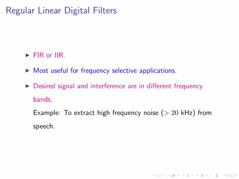
Regular Linear Digital Filters

◮ FIR or IIR.

◮ Most useful for frequency selective applications.

◮ Desired signal and interference are in different frequency

bands.

Example: To extract high frequency noise (> 20 kHz) from

speech.

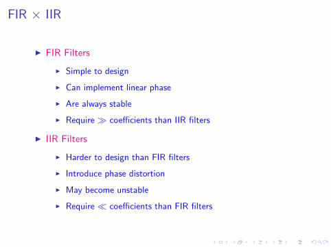
FIR × IIR

◮ FIR Filters

◮ Simple to design

◮ Can implement linear phase

◮ Are always stable

◮ Require ≫ coefficients than IIR filters

◮ IIR Filters

◮ Harder to design than FIR filters

◮ Introduce phase distortion

◮ May become unstable

◮ Require ≪ coefficients than FIR filters

Statistical Linear Filtering

◮ Many applications → more than just frequency band selection

◮ Signal and interference are frequently within the same freq.

band

◮ Solution is based on the statistical properties of the signals

Basic Operations in Linear Filtering

1. Filtering

Extraction of information at a given time n by using data

measured before and at time n.

2. Smoothing

Differs from filtering in that data measured both before and

after n can be used to extract information at time n.

3. Prediction

Predicts how the quantity of interest will be at time n + N for

some N > 0 by using data measured up to and including n.

(The filter is linear if its output is a linear function of the

observations applied to the input.)

How Do We Do Linear Statistical Filtering?

◮ We assume some statistical properties of the useful and

unwanted signals are available

Mean Autocorrelation Cross-correlations etc.

◮ We define some statistical criterion for the optimization of the

filter performance

Optimal Linear Filtering

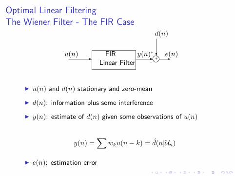
The Wiener Filter - The FIR Case

++

−

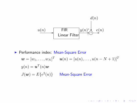
u(n) FIRLinear Filter

y(n)

d(n)

e(n)

◮ u(n) and d(n) stationary and zero-mean

◮ d(n): information plus some interference

◮ y(n): estimate of d(n) given some observations of u(n)

y(n) =∑

wku(n − k) = d(n|Un)

◮ e(n): estimation error

++

−

u(n) FIRLinear Filter

y(n)

d(n)

e(n)

◮ Performance index: Mean-Square Error

w = [w1, . . . , wN ]T u(n) = [u(n), . . . , u(n − N + 1)]T

y(n) = uT (n)w

J(w) = E{e2(n)} Mean-Square Error

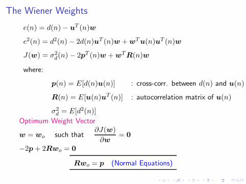
The Wiener Weights

e(n) = d(n) − uT (n)w

e2(n) = d2(n) − 2d(n)uT (n)w + wT u(n)uT (n)w

J(w) = σ2d(n) − 2pT (n)w + wT R(n)w

where:

p(n) = E[d(n)u(n)] : cross-corr. between d(n) and u(n)

R(n) = E[u(n)uT (n)] : autocorrelation matrix of u(n)

σ2d = E[d2(n)]

Optimum Weight Vector

w = wo such that∂J(w)

∂w= 0

−2p + 2Rwo = 0

Rwo = p (Normal Equations)

−20 −10 0 10 20

−20−10

010

200

500

1000

1500

2000

2500

3000

3500

w1

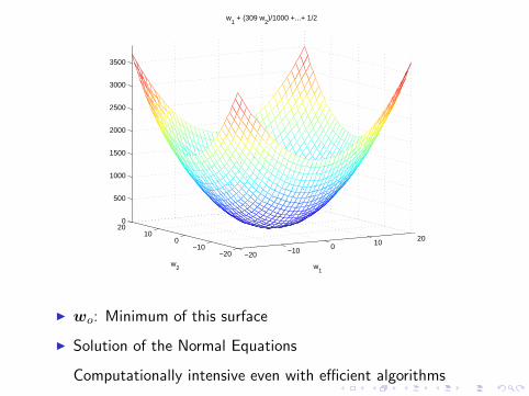
w1 + (309 w

2)/1000 +...+ 1/2

w2

◮ wo: Minimum of this surface

◮ Solution of the Normal Equations

Computationally intensive even with efficient algorithms

60

What is an Adaptive Filter Anyway?

In several practical real-time applications:

◮ The signal involved are nonstationary

◮ Normal equations must be solved for each n!?!

◮ The algorithms used for the stationary case become inefficient

◮ What about Kalman Filters?

◮ Requires a dynamics model (state-space) for d(n)

◮ Computationally heavy for real-time

◮ Signal statistics may be unknown, and there may be no time

to estimate them

◮ Computational complexity between 2 input samples limited by

processor speed and by cost

Adaptive Filters

◮ Change their weights as new input samples arrive

◮ Weight updating is controlled by an adaptive algorithm

◮ Optimal solution is approached by improving performance a

little bit at each iteration

◮ Optimal solution is approximated after several iterations

(iteration complexity × convergence time)

◮ Filter weights become random variables that converge to a

region about the optimum weights

◮ Can track signal and system nonstationarities

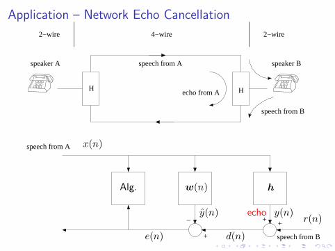
Application – Network Echo Cancellation

H

2−wire 4−wire 2−wire

speaker A speaker Bspeech from A

speech from B

echo from AH

speech from A

speech from B

++

+

_

x(n)

Alg. w(n) h

y(n)

d(n)

r(n)y(n)

e(n)

echo

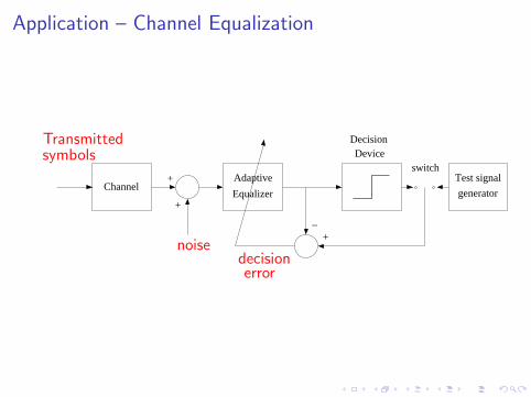
Application – Channel Equalization

ChannelAdaptive

Equalizer

DecisionDevice

Test signal

generator

+

+

+

_

switch

Transmittedsymbols

noisedecisionerror

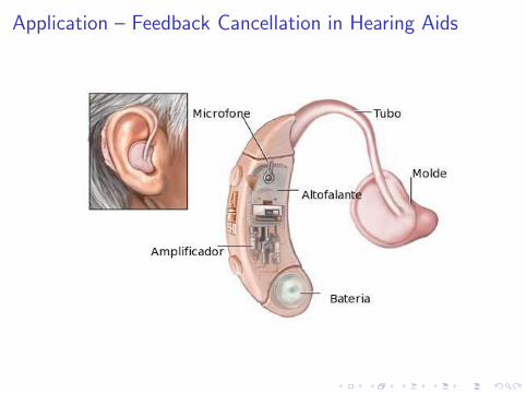
Application – Feedback Cancellation in Hearing Aids

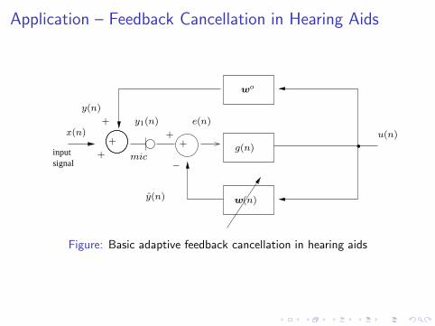
Application – Feedback Cancellation in Hearing Aids

inputsignal

+

+

+−

u(n)

wo

y1(n)

y(n)

++

e(n)

y(n)w(n)

x(n)

g(n)mic

Figure: Basic adaptive feedback cancellation in hearing aids

Adaptive Algorithm - Least Mean Squares (LMS)

Optimization Problem

Determine w that minimizes

J(w)|w=w(n) = σ2

d(n) − 2pT (n)w(n) + w(n)T R(n)w(n)

Steepest Descent Algorithm

Direction contrary to the gradient∂J(w)

∂w

∂J(w)

∂w= −2p + 2Rw(n)

w(n + 1) = w(n) + µ[p − Rw(n)]

(µ controls de adaptation speed)

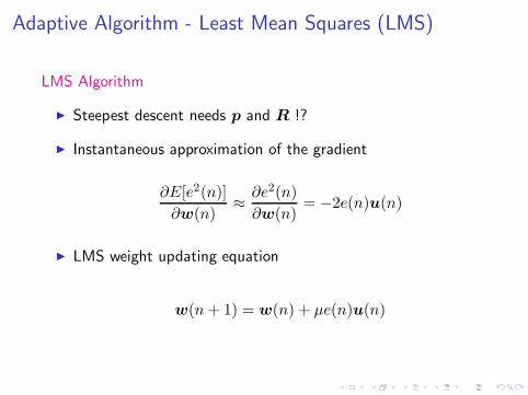
Adaptive Algorithm - Least Mean Squares (LMS)

LMS Algorithm

◮ Steepest descent needs p and R !?

◮ Instantaneous approximation of the gradient

∂E[e2(n)]

∂w(n)≈

∂e2(n)

∂w(n)= −2e(n)u(n)

◮ LMS weight updating equation

w(n + 1) = w(n) + µe(n)u(n)

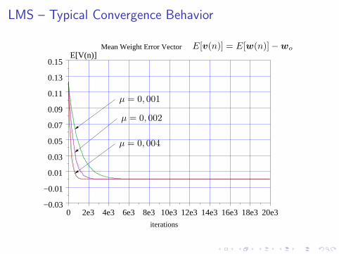
LMS – Typical Convergence Behavior

iterations

Mean Weight Error Vector

0 2e3 4e3 6e3 8e3 10e3 12e3 14e3 16e3 18e3 20e3−0.03

−0.01

0.01

0.03

0.07

0.09

0.11

0.13

0.15E[V(n)]

0.05

E[v(n)] = E[w(n)] − wo

µ = 0, 001

µ = 0, 002

µ = 0, 004

LMS – Typical Convergence Behavior

0 2e3 4e3 6e3 8e3 10e3 12e3 14e3 16e3 18e3 20e3−110

−90

−70

−50

−30

−10

10

30

Mean−Square ErrorMSE (dB)

iterations

µ = 0, 001

µ = 0, 002

µ = 0, 004