Master’s Degreein Computer Science - Software Dependability andCyber SecuritySecond Cycle (D.M. 270/2004)

Computer Science Master’s Thesis

Adaptive query handler for ORMtechnologies

SupervisorAndrea Marin

GraduandPaolo Quartarone,859724

Year2019/2020

2

Abstract

In modern software engineering, the mapping between the software layer andthe persistent data layer is handled by the Object Relational Mapping (ORM)tools. These transform the operations on objects into DBMS CRUD queries.The problem of formulating the query associated with the operations in themost efficient way has been only partially solved by static code annotations.This implies that the programmer must guess the behavior of the softwareonce it is deployed in order to choose the best configuration. In this work,we make a step toward the dynamic configuration of the queries. The ORMwe propose aims to improve the overall system performance monitoring andadapting the behavior of the query. The solution achieves the result bypruning the query in two steps. In the first step, the ORM chooses thecolumns to fetch, taking into account the system load and usage frequencies.In the second step it exploits the join elimination optimization. This is afeature implemented by some DBMS that removes unnecessary tables from aquery, avoiding useless scans and join operations. Then, the ORM proposedapplies together eager and lazy strategies. It loads the expected data eagerly,and it loads lazily the data not expected but subsequently requested. Theefficiency of the proposed solution is assessed through customized tests andthrough the Tsung benchmark tool, comparing the ORM developed with asimple JDBC connection and the Hibernate ORM service.

Keywords: ORM, Java, performance, queueing systems, database, soft-ware engineering

Contents

1 Introduction 51.1 Problem description . . . . . . . . . . . . . . . . . . . . . . . . 51.2 State of art solutions . . . . . . . . . . . . . . . . . . . . . . . 6

1.2.1 Evaluation strategy . . . . . . . . . . . . . . . . . . . . 61.2.2 ORM tools . . . . . . . . . . . . . . . . . . . . . . . . 81.2.3 Auto-Fetch . . . . . . . . . . . . . . . . . . . . . . . . 11

1.3 Proposed solution . . . . . . . . . . . . . . . . . . . . . . . . . 121.4 Document content . . . . . . . . . . . . . . . . . . . . . . . . 13

2 Theoretical Background 152.1 Database . . . . . . . . . . . . . . . . . . . . . . . . . . . . . . 15

2.1.1 Relational database . . . . . . . . . . . . . . . . . . . . 162.1.2 NoSQL . . . . . . . . . . . . . . . . . . . . . . . . . . . 162.1.3 SQL vs NoSQL . . . . . . . . . . . . . . . . . . . . . . 17

2.2 Object Oriented Programming . . . . . . . . . . . . . . . . . . 172.2.1 Patterns . . . . . . . . . . . . . . . . . . . . . . . . . . 18

2.3 Multitier Architecture . . . . . . . . . . . . . . . . . . . . . . 192.4 Queueing system . . . . . . . . . . . . . . . . . . . . . . . . . 20

2.4.1 Little’s Law . . . . . . . . . . . . . . . . . . . . . . . . 222.4.2 PASTA Property . . . . . . . . . . . . . . . . . . . . . 23

2.5 Queueing networks . . . . . . . . . . . . . . . . . . . . . . . . 232.5.1 Open Network . . . . . . . . . . . . . . . . . . . . . . . 242.5.2 Closed Network . . . . . . . . . . . . . . . . . . . . . . 24

2.6 Performance testing . . . . . . . . . . . . . . . . . . . . . . . . 262.7 Statistical inference . . . . . . . . . . . . . . . . . . . . . . . . 27

2.7.1 Hypothesis Testing . . . . . . . . . . . . . . . . . . . . 27

1

3 Implementation of AdaORM 313.1 Software . . . . . . . . . . . . . . . . . . . . . . . . . . . . . . 31

3.1.1 Programming language . . . . . . . . . . . . . . . . . . 313.1.2 Database . . . . . . . . . . . . . . . . . . . . . . . . . 313.1.3 Frameworks . . . . . . . . . . . . . . . . . . . . . . . . 323.1.4 Libraries . . . . . . . . . . . . . . . . . . . . . . . . . . 323.1.5 Patterns . . . . . . . . . . . . . . . . . . . . . . . . . . 323.1.6 Main functionalities . . . . . . . . . . . . . . . . . . . . 343.1.7 Conclusion . . . . . . . . . . . . . . . . . . . . . . . . . 40

4 Experiments and Analysis of AdaORM 414.1 Network architecture . . . . . . . . . . . . . . . . . . . . . . . 41

4.1.1 Application Server . . . . . . . . . . . . . . . . . . . . 424.1.2 Database Server . . . . . . . . . . . . . . . . . . . . . . 43

4.2 Databases Benchmark . . . . . . . . . . . . . . . . . . . . . . 444.2.1 Join Elimination optimization . . . . . . . . . . . . . . 454.2.2 MySQL . . . . . . . . . . . . . . . . . . . . . . . . . . 454.2.3 PostgreSQL . . . . . . . . . . . . . . . . . . . . . . . . 494.2.4 DB2 . . . . . . . . . . . . . . . . . . . . . . . . . . . . 504.2.5 Conclusion . . . . . . . . . . . . . . . . . . . . . . . . . 52

4.3 Application Benchmarks . . . . . . . . . . . . . . . . . . . . . 534.3.1 Configuration . . . . . . . . . . . . . . . . . . . . . . . 544.3.2 Database . . . . . . . . . . . . . . . . . . . . . . . . . 554.3.3 Custom benchmark . . . . . . . . . . . . . . . . . . . . 564.3.4 Web Server benchmark with Tsung . . . . . . . . . . . 614.3.5 Comparison of AdaORM and Hibernate . . . . . . . . . . 72

4.4 Queueing system analysis . . . . . . . . . . . . . . . . . . . . 764.4.1 Adaptive Heavy Query . . . . . . . . . . . . . . . . . . 764.4.2 JDBC Heavy Query . . . . . . . . . . . . . . . . . . . 804.4.3 Conclusion . . . . . . . . . . . . . . . . . . . . . . . . . 84

4.5 Prototype limits . . . . . . . . . . . . . . . . . . . . . . . . . . 844.5.1 Concurrency . . . . . . . . . . . . . . . . . . . . . . . . 854.5.2 System database . . . . . . . . . . . . . . . . . . . . . 854.5.3 Usability . . . . . . . . . . . . . . . . . . . . . . . . . . 85

5 Conclusions and Future Works 875.1 Data prediction . . . . . . . . . . . . . . . . . . . . . . . . . . 885.2 Cost impact . . . . . . . . . . . . . . . . . . . . . . . . . . . . 88

2

6 Acknowledgements 91

3

4

Chapter 1

Introduction

1.1 Problem descriptionNowadays, exist some interesting methodologies to allow communication be-tween software layer and data layer. Avoiding verbose code to fetch data fromthe last layer, it is possible to use the Object Relational Mapping (ORM)tools. These tools implement ORM programming paradigm to favor theintegration among object oriented programming languages (OOP) and rela-tion database management system (RDBMS). ORM tools try to solve theproblem of formulating the query associated with the operations in the mostefficient way by static code annotations. This implies that the programmermust guess the behavior of the software once it is written in order to choosethe best configuration. A wrong static choice will lead to an unnecessarywaste in terms of computation time and resources used, these degrade per-formance. For example, the developer chooses statically a query that loads abig result set but the user always uses only some values. In this case, wherethe user only needs a small amount of data, our application, set statically,loads a lot of them anyway. With this strategy our developer has a heavyapplication, which response time is higher than the optimal time. Then, thedeveloper chooses a cheaper static approach, at least at the beginning. Hechooses to load only values that user asks. This can improve response timeat the beginning, but if the user runs a routine that requires all informationhe will load each parameter individually, giving a big waste of time. Then hedecides to study the entire system to decide how and where the applicationmust load a bigger result set and where a smaller one. But the system is

5

too complex and in continuous evolution. In this case, the developer mustanalyze and maintain too many cases, increasing developing time and costs.

In this thesis we present AdaORM , an ORM prototype that aims to improvedata fetch from database using a new strategy that handles the query afterthe observation of its behavior. AdaORM also allows to reduce the developmentand maintenance times of the application, thus makes the development ofthe application cheaper. AdaORM automatically chooses the most probablequery to submit to RDBMS according to observed behaviors of the query andparameters utilization. To achieve the goal, AdaORM performs optimization intwo steps. In the first step, it collects statistics over query columns usage andchooses dynamically what of them can be removed from the query statement.In the second step, after the submission of the new edited statement tothe DBMS, AdaORM exploits the join elimination optimization, a featureimplemented by some DBMS that removes not useful tables from the query,avoiding unnecessary scans and join operations. AdaORM is able to improvequery execution times because DBMS works with less tables, it improvessystem response time because AdaORM handles less data and, at the end, itreduces the system load.

1.2 State of art solutionsIn this section we describe firstly state-of-art strategies that ORM tools,persistence framework and active record database pattern implement. Forsimplicity, we always talk about these three solution as ORM tool. In fact weare interested to understand how they works and how they try to optimizedata fetch. The strategies are described by treating their strengths andweaknesses, demonstrating on which cases they are the best choice and inwhich the worst one. Then, we talk about the most famous ORM solutions.ORMs are described according to their purpose, their strategies and theirfunctions used to achieve it. So let’s describe their strengths and weaknesses.At the end, we talk about an interesting technique called AutoFetch thatgenerates automatically prefetching using transversal profiling.

1.2.1 Evaluation strategy

Evaluation strategy changes the behavior of execution flow according to theevaluation chosen. An evaluation strategy decides when and how evaluate

6

an expression that is bound to a variable. Applying an evaluation strategyto an ORM changes its behavior according to the static setting defined bythe developer. To understand better how a ORM tool works is important tounderstand how the applied evaluation strategy works.

Strict evaluation: called also eager evaluation, is an evaluation strategywhich evaluates as soon as possible the expression that is bound to a vari-able. Using this strategy it improves code workflow and facility the debug.However, eager evaluation can reduce performance in case of too many andunnecessary evaluations.

An ORM tool that uses this kind of strategy loads immediately all val-ues from the goal table and also loads immediately all values from relationone-to-many. Only many-to-many relations will be performed after request-ing. An application that implements an ORM with this strategy providesslower response times following an object request, but it has no delay whenasked to return the value of an object property with one-to-many relation-ship. Avoiding making new connections to the database, the application ismuch faster providing the required value. However, if the loaded values fromrelations are never used, we can interpret this situation as a waste of timeand system resource.

Non-strict evaluation: also called lazy evaluation, is an evaluation strat-egy which evaluates expressions bound to a variable only in the moment theyare required to complete the execution flow, correctly. This strategy allowsto improve performance in the opposite situation of eager evaluation. In fact,in case we need the results of all evaluations and the strategy that we areusing is lazy, we have worse performance.

An ORM tool that uses this kind of strategy will load immediately allvalues from the goal table and, when requested, the values from other tablewith relations one-to-many or many-to-many. ORMs tool that works withthis strategy responds faster when a client requests the object fetch, but itresponds slower when it asks to return values from one-to-many relations.The performance in this case degrades because ORM tool must pay somefixed time in database connection, even if there is little data to load. However,if the loaded values from relations will be never used, we can interpret thissituation as a gain of time and system resources.

7

Non-deterministic evaluation In this evaluation strategy arguments areloaded after heuristics evaluations at run-time. We cannot know how theworkflow will be. These family of evaluation strategies can give high per-formance improvement, but its result might provide unexpected values. De-bugging can be complicated and the execution flow is decided when choosingwhether to evaluate an expression or not.

AdaORM implements a predictive evaluation strategy that can be mappedin this macro strategy.

1.2.2 ORM tools

Object-Relational Mapping (ORM) is a programming technique that aimsto improve integration among software system, that uses object orientedparadigm and RDBMS systems, creating a virtual object database. A ORMtool solves the problem of translating the information to be stored in a re-lational database, preserving the properties and relationships that involveobject in OOP paradigm. Those tools load data from databases accordingto the chosen evaluation strategy.

Advantages: by introducing this kind of technology, we obtain some ad-vantages. As the reduction of the code to write. The less we write, the lesserror we make. Also, development time is reduced and we are able to avoidboilerplate code. Using an ORM improves the portability over the DBMSused. Only changing some lines of code and importing the correct driver wecan use one specific language instead of SQL.

Disadvantages: there are some unfavorable points. The higher level ofabstraction doesn’t show what happens inside. Sometimes, it can be usefulmaking the process transparent. Other times, it doesn’t give enough infor-mation and/or control to improve the behavior of an application. The lastdisadvantage is the main point that we want to improve with AdaORM .

Also, an ORM tool helps the developer with other features like auto-matic object graph loading, concurrency management, caching support andimprovement on DBMS communication.

8

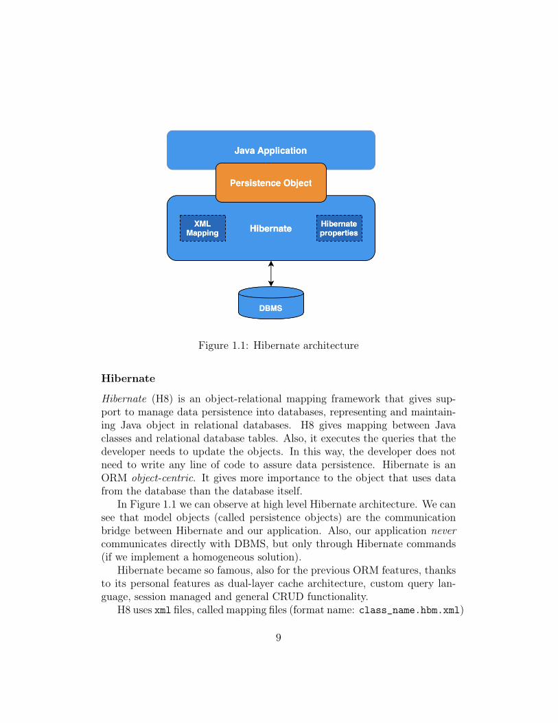
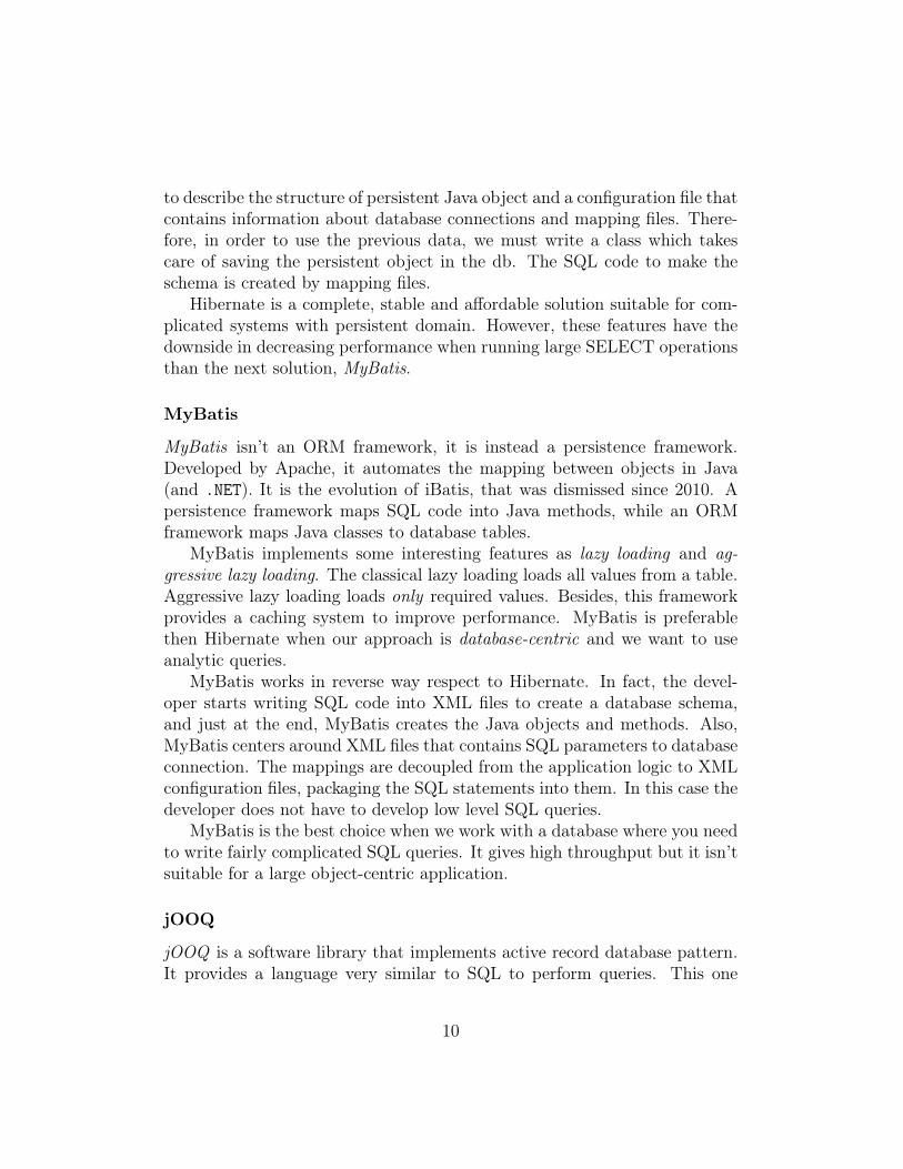
Figure 1.1: Hibernate architecture

Hibernate

Hibernate (H8) is an object-relational mapping framework that gives sup-port to manage data persistence into databases, representing and maintain-ing Java object in relational databases. H8 gives mapping between Javaclasses and relational database tables. Also, it executes the queries that thedeveloper needs to update the objects. In this way, the developer does notneed to write any line of code to assure data persistence. Hibernate is anORM object-centric. It gives more importance to the object that uses datafrom the database than the database itself.

In Figure 1.1 we can observe at high level Hibernate architecture. We cansee that model objects (called persistence objects) are the communicationbridge between Hibernate and our application. Also, our application nevercommunicates directly with DBMS, but only through Hibernate commands(if we implement a homogeneous solution).

Hibernate became so famous, also for the previous ORM features, thanksto its personal features as dual-layer cache architecture, custom query lan-guage, session managed and general CRUD functionality.

H8 uses xml files, called mapping files (format name: class_name.hbm.xml)

9

to describe the structure of persistent Java object and a configuration file thatcontains information about database connections and mapping files. There-fore, in order to use the previous data, we must write a class which takescare of saving the persistent object in the db. The SQL code to make theschema is created by mapping files.

Hibernate is a complete, stable and affordable solution suitable for com-plicated systems with persistent domain. However, these features have thedownside in decreasing performance when running large SELECT operationsthan the next solution, MyBatis.

MyBatis

MyBatis isn’t an ORM framework, it is instead a persistence framework.Developed by Apache, it automates the mapping between objects in Java(and .NET). It is the evolution of iBatis, that was dismissed since 2010. Apersistence framework maps SQL code into Java methods, while an ORMframework maps Java classes to database tables.

MyBatis implements some interesting features as lazy loading and ag-gressive lazy loading. The classical lazy loading loads all values from a table.Aggressive lazy loading loads only required values. Besides, this frameworkprovides a caching system to improve performance. MyBatis is preferablethen Hibernate when our approach is database-centric and we want to useanalytic queries.

MyBatis works in reverse way respect to Hibernate. In fact, the devel-oper starts writing SQL code into XML files to create a database schema,and just at the end, MyBatis creates the Java objects and methods. Also,MyBatis centers around XML files that contains SQL parameters to databaseconnection. The mappings are decoupled from the application logic to XMLconfiguration files, packaging the SQL statements into them. In this case thedeveloper does not have to develop low level SQL queries.

MyBatis is the best choice when we work with a database where you needto write fairly complicated SQL queries. It gives high throughput but it isn’tsuitable for a large object-centric application.

jOOQ

jOOQ is a software library that implements active record database pattern.It provides a language very similar to SQL to perform queries. This one

10

allows to implement some functionalities that cannot be used with otherORM, staying very light. jOOQ has a database-centric approach, as we couldimagine from its syntax. The syntax allows to standardize the language, inthis way it will be independent from under RDBMS layer. Also, jOOQ ismulti-tenancy, it works using many instance of the same service in a sharedenvironment.

jOOQ abstracts SQL through some function. In this way we becomeindependent from the under DB and we are less exposed to risk. It supportsmany SQL features that cannot be used with other ORM. In fact, ORMsuch as Hibernate, are expensive resources and they don’t permit all SQLoperations. jOOQ is very different than Hibernate and MyBatis. It givesto the developer a lot of control, which in inexperienced hands can lead toserious performance problems. jOOQ implements eager loading by default.This means that if you are using a large database and you are loading a lotof data, which of then might not be all used, it will lead to an unnecessarywaste of time and resources.

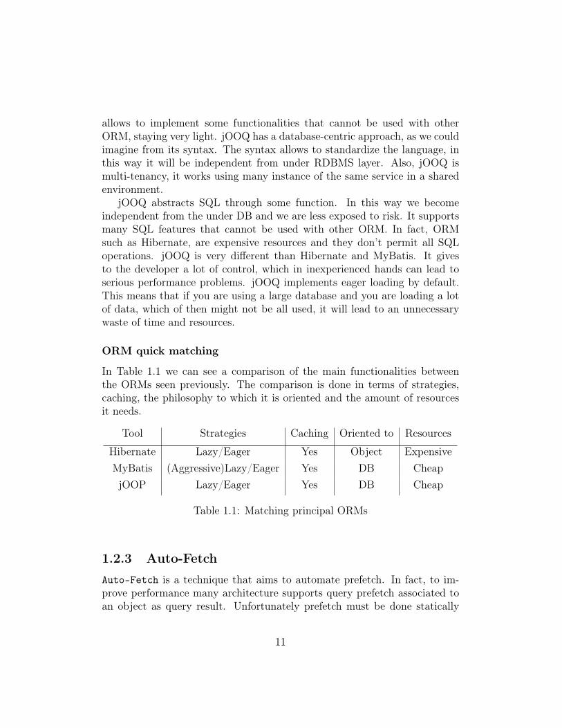
ORM quick matching

In Table 1.1 we can see a comparison of the main functionalities betweenthe ORMs seen previously. The comparison is done in terms of strategies,caching, the philosophy to which it is oriented and the amount of resourcesit needs.

Tool Strategies Caching Oriented to Resources

Hibernate Lazy/Eager Yes Object ExpensiveMyBatis (Aggressive)Lazy/Eager Yes DB CheapjOOP Lazy/Eager Yes DB Cheap

Table 1.1: Matching principal ORMs

1.2.3 Auto-Fetch

Auto-Fetch is a technique that aims to automate prefetch. In fact, to im-prove performance many architecture supports query prefetch associated toan object as query result. Unfortunately prefetch must be done statically

11

in the code and sometimes might be difficult to guess the correct query ofmaintain it, mostly in modular system. Auto-fetch achieves this resultthrough the traversal profiling1 in object persistence architecture. This tech-nique based its prefetch over previous query executions of similar queries.Auto-fetch records traversed associations when we submit a query. Then,recorded information are aggregated to profile a statistical application be-havior. It can prefetches arbitrary transversal patterns. In this way, theapplication performs less queries, improving performance. Auto-fetch mapsexecution flow with a graph, because is the natural representation of relationsin most object persistence architectures. Auto-fetch understands only afterone execution how to prefetch correctly a query. In fact, from the second ex-ecution it is already able to execute the best prefetch. However, it classifiesonly on the criteria, without distinguish the different query utilization. Inthis case the classification is too coarse. Furthermore, Auto-fetch does notimplement the feature to perform lighter prefetch if the load on the systemis higher. It also can possibly aggravating the system load.

1.3 Proposed solutionThe contribution of this thesis is the development of an ORM prototype,AdaORM , that aims to improve system response time and system load. AdaORMuses a predictive strategy that exploits collected statistics and a feature im-plemented in some DBMS, join elimination optimization. join eliminationprunes query statement removing useless tables. In this document we assessthrough customized benchmark test and using Tsung benchmark tool, howthe system response time, the complexity of executed query and system loaddecrease exploiting the features offered by AdaORM .

Achieving the fixed goals is possible to exploit a particular feature im-plemented from a some DBMS, the join elimination optimization. Thisoptimization removes unnecessary tables from a submitted query. In thisway, the DBMS performs less operation, decreasing the query cost and im-proving the response time. Before AdaORM , the developer was forced to hardcode different query for different execution contexts to improve performance,handling the query each time that the system behavior changes. Then, main-taining system efficient and performing each time that the behavior changes,has an expensive cost in term of maintenance and complexity. Now, thanks

1transversal profiling is a technique to collect statistics tracking the control flow.

12

to AdaORM we are able to solve these problems. It works observing the behav-ior of requested query and the mapped column utilization. By the using ofcollected statistics on the application behavior, AdaORM formulates the querystatement by removing the columns which are not evaluated as interesting.Ranges are set up monitoring the current system load. When we reload theinterrogation we have to check the fixed system load. If a column frequencyusage is enough high and according to the full system usage, it is loaded intothe final query.

The tables are not removed by AdaORM but only from DBMS that imple-ments join elimination .

1.4 Document contentIn the first chapter we described the problems that we aim to face, howto improve application response time and save resources. We described thestate-of-art solutions and how they try to solve the problem or someshades of it. Then, we briefly described AdaORM , the proposed solution toprevious problems.

In the second part we give some theoretical knowledge about databases,that are the heart of the problem. Then we describe the Object OrientedProgramming, a programming paradigm to develop structured and modularapplications. After that, we talk about Object Relational Mapping, a pro-gramming technique to improve integrity and develop time among relationaldatabase and Object Oriented Programming, with some principal solutions.Then, we introduce the multitier architecture, a way to describe a particulartype of client-server architecture, to pass after that to talk about queueingnetworks and how to perform performance testing. At the end, we spendsome words to describe the statistical methods that we want to use to assessthe performance improvement given by AdaORM .

In chapter 3 we describe how we implemented AdaORM , describing softwareand hardware components. This chapter is necessary to understand betterthe subsequent one.

In chapter 4 we show the experiments done with different databases toassess the performance improvement gained having the join elimination. Then, we comment some plots obtained from benchmark results of AdaORM. Benchmarks have been done with a custom benchmark and with Tsung inserver configuration. We compare AdaORM with Hibernate and we show some

13

cases of study where the proposed solution overcome Hibernate executiontime. At the end, we give some limits found in my prototype.

In the last chapter we give a last observation over the project and wepropose interesting possible future works to be implemented on AdaORM, fo-cusing on improving data prediction and reducing the computation cost ofthe application layer.

14

Chapter 2

Theoretical Background

To make this self-contained thesis we decided to theoretically introduce themain topics that will be covered. In the next sections we will talk aboutdatabases, that are a key point of our research. We will introduce the ObjectOriented Programming (OOP) paradigm and we will describe principal pat-tern used. After that, we will talk about Object Relational Mapping (ORM),a technique that allows us to link together two different paradigm as RDBMSand OOP. Then, we will describe Multi-tier architecture to represent a par-ticular type of client-server architecture. Studying and testing the adoptedsystem will be possible thanks to Queueing system network, described below.At the end, we will give some theoretical definition over statistics methodsthat we will use to assess the obtained improvements.

2.1 DatabaseIn this section, we will talk about the two families of databases and theirprincipal features.

A database is a collection of data, organized and electronically storedover a computer system.[1] Interacting with a database is possible thanksto the database management system (DBMS). A DBMS is a software layerthat allows users and applications to interact with data layer. According todatabase model, that determines the database logical structure and defineshow data can be stored, organized and manipulated, we split DBMS in twofamilies: Relational database and NoSQL.

15

2.1.1 Relational database

Relational database is a database structured over the concept of relation. It ispossible to interact with a relational database thanks to Relational DatabaseManagement System (RDBMS). Data are presented to the end user and ap-plication as relations of tables. Each table consists of a set of rows, called alsorecords or tuple; and columns, that are the attribute which value describesrows. Each row is uniquely identifiable into the system through the use of aprimary key (PK), a particular attribute or set of attributes that are uniquein the table. PK can be used also as foreign key (FK) to link together rowsand to make relation among them.

SQL: acronym of Structured Query Language, is the query language usedto interact with a RDBMS. A RDBMS can extend SQL with many otherfeatures as new commands or attribute type. This extension takes the nameof dialect.

2.1.2 NoSQL

A NoSQL database is a system that provides methods to store and to retrieveinformation in different ways which are not the classic relational models.NoSQL database can be split in different families that depend from the typeof data model they work with. The most used data models are documentgraph, key-value and wide-column. Using NoSQL databases can offer someadvantages, as design simplicity, flexibility working with unstrucutured data,simpler "horizontal" scaling to cluster, but NoSQL database has an high im-pact over the amount of memory to storage data. However, the cost to storedata is a convenient cost because its simplicity decreases the developmentcosts. Now we explain better the difference between data model used byNoSQL databases.

Document databases: data are stored into document as JSON. Into thedocument we can find a couple of key-value. Values have type, that can beprimitive, or complex type as object. Sometimes, object/variable type intodocument are the same used by programming language used. This simplifiesthe mapping between data into document and classes.

16

Graph databases: data are stored as a graph, where node represent valuesand edges represent the relations among them. Graph representation is aconvenient choice when we have to work with algorithms that nativity requirehandling graph.

Key-value databases: data are memorized in couples key-value. The keyis used to retrieve information linked with it. Key-value is a convenient rep-resentation when we need to retrieve quickly a value, but we do not performcomplex query over our database.

Wide-column stores: data are saved in tables, rows, and dynamic columns.Wide-column is like a relational database, but it provides a lot of flexibilitybecause each row is not required to have the same columns. Wide-columnis a convenient representation when you need to memorize large amounts ofdata and you can predict what your query patterns are.

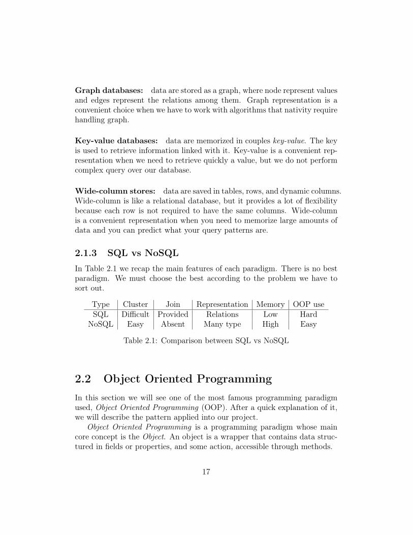
2.1.3 SQL vs NoSQL

In Table 2.1 we recap the main features of each paradigm. There is no bestparadigm. We must choose the best according to the problem we have tosort out.

Type Cluster Join Representation Memory OOP useSQL Difficult Provided Relations Low Hard

NoSQL Easy Absent Many type High Easy

Table 2.1: Comparison between SQL vs NoSQL

2.2 Object Oriented ProgrammingIn this section we will see one of the most famous programming paradigmused, Object Oriented Programming (OOP). After a quick explanation of it,we will describe the pattern applied into our project.

Object Oriented Programming is a programming paradigm whose maincore concept is the Object. An object is a wrapper that contains data struc-tured in fields or properties, and some action, accessible through methods.

17

2.2.1 Patterns

We can define a pattern as a reusable solution to frequently current problems.Exploiting pattern is the best way to develop good codes. In this documentwe will see only pattern that we used developing AdaORM [7].

Strategy: is a behavioral pattern that allows to choose the right algorithmat runtime. Delegating the algorithm choice at runtime, it improves thecode reusability. Validation algorithm and validating object are encapsulatedseparately. In this way we can validate the same object in different contextswithout duplication codes.

Figure 2.1: UML representation of Strategy pattern

In Figure 2.1 we can observe how the Context class does not implementdirectly any action, but delegates its implementation to others classes. Infact, implementing Strategy interface, the Context will be able to change itsbehavior dynamically, changing the referred strategy. Classes RealStrategyAand RealStrategyB implement the Strategy class, then the algorithm thatwill be executed.

Decorator: aims to solve the problem of how adding/removing object re-sponsible dynamically or at runtime, avoiding subclassing explosion.

Decorator does not change the behavior of original class, but wraps it.How we can see in Figure 2.2, Decorator class has an attribute that is of thesame type as the class that extends. In this way Decorator, also appears as

18

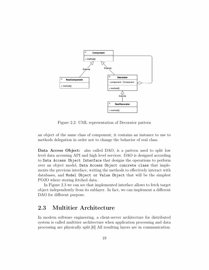
Figure 2.2: UML representation of Decorator pattern

an object of the same class of component, it contains an instance to use tomethods delegation in order not to change the behavior of real class.

Data Access Object: also called DAO, is a pattern used to split lowlevel data accessing API and high level services. DAO is designed accordingto Data Access Object Interface that designs the operations to performover an object model, Data Access Object concrete class that imple-ments the previous interface, writing the methods to effectively interact withdatabases, and Model Object or Value Object that will be the simplestPOJO where storing fetched data.

In Figure 2.3 we can see that implemented interface allows to fetch targetobject independently from its sublayer. In fact, we can implement a differentDAO for different purpose.

2.3 Multitier ArchitectureIn modern software engineering, a client-server architecture for distributedsystem is called multitier architecture when application processing and dataprocessing are physically split.[6] All resulting layers are in communication.

19

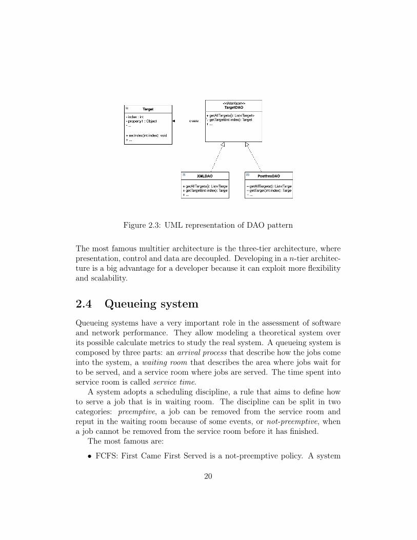
Figure 2.3: UML representation of DAO pattern

The most famous multitier architecture is the three-tier architecture, wherepresentation, control and data are decoupled. Developing in a n-tier architec-ture is a big advantage for a developer because it can exploit more flexibilityand scalability.

2.4 Queueing systemQueueing systems have a very important role in the assessment of softwareand network performance. They allow modeling a theoretical system overits possible calculate metrics to study the real system. A queueing system iscomposed by three parts: an arrival process that describe how the jobs comeinto the system, a waiting room that describes the area where jobs wait forto be served, and a service room where jobs are served. The time spent intoservice room is called service time.

A system adopts a scheduling discipline, a rule that aims to define howto serve a job that is in waiting room. The discipline can be split in twocategories: preemptive, a job can be removed from the service room andreput in the waiting room because of some events, or not-preemptive, whena job cannot be removed from the service room before it has finished.

The most famous are:

• FCFS: First Came First Served is a not-preemptive policy. A system

20

set with this rule will serve before the job, according to their arrivalorder.

• LCFS: Last Came First Server is a preemptive policy. A system setwith this discipline will serve job on inverse arrival order.

• RR: Round Robin is a preemptive discipline. The system spends acertain amount of time for each job.

• SJF: Short Job First discipline is a preemptive rule that aims to max-imize throughput serving first shorter jobs.

• SRTP: Shortest Remaining Processing Time is a preemptive disciplinewith resume that serves always the job that has the shortest comple-tation time. It tries to minimize the response time.

• RAND: policy not-preemptive that chooses randomly a job wheneverthe server is free.

Describing a queueing system can be very verbose. It is possible to avoidthis issue using Kendall’s notation. A system can be described using a stringas A/B/m/K/P/D where:

• A and B describe the inter-arrival times and the distribution of theservice times of jobs. A and B can be replaced with the followingletters to describe the distribution type:

– M denotes the exponential distribution. If M replaces A the rep-resents the Poisson distribution.

– D describes the deterministic distribution.

– G denotes the general distribution. It is in most of the generalcase.

– many others

• m is the number of identical servers in the system.

• K represents the capacity of the queue.

• P describes the population size.

• D is the scheduling discipline.

21

For example, M/M/1 is the Kendall’s notation to describe a system withPoisson distribution at arrival process, exponential distribution at departureprocess and one server, with infinite capacity and infinity population, andthe scheduling discipline is FCFS.

To study a queueing system it is necessary to introduce some performanceindices that describe some particular behavior of the case of study.

• N(t) is the number of jobs in the system in a certain epoch t.

• W is the random variable that describes the waiting time of a job intothe waiting room.

• S is the service time of a job.

• µ is the service rate. E[s] = µ−1.

• R is the amount of time that a job spends into the system. R = W +S.

• λ is the arrival rate of a job into the system.

• U is the utilization of a single system queue defined as U = λµ

2.4.1 Little’s Law

Little’s Law is one of the most important result in queueing system theory.It requires very few constraints to be applied. In fact, it is independentfrom arrival/departure distribution used to describe the system, but it allowshowever to calculate the number of jobs in a system in a defined time t.

Little’s law: A queueing system without internal loss or generation of jobsis given, then the following relation holds for any finite time t:

N(t) = R(t)X(t)

From the previous law we can deduce the next theorem setting t→∞.

22

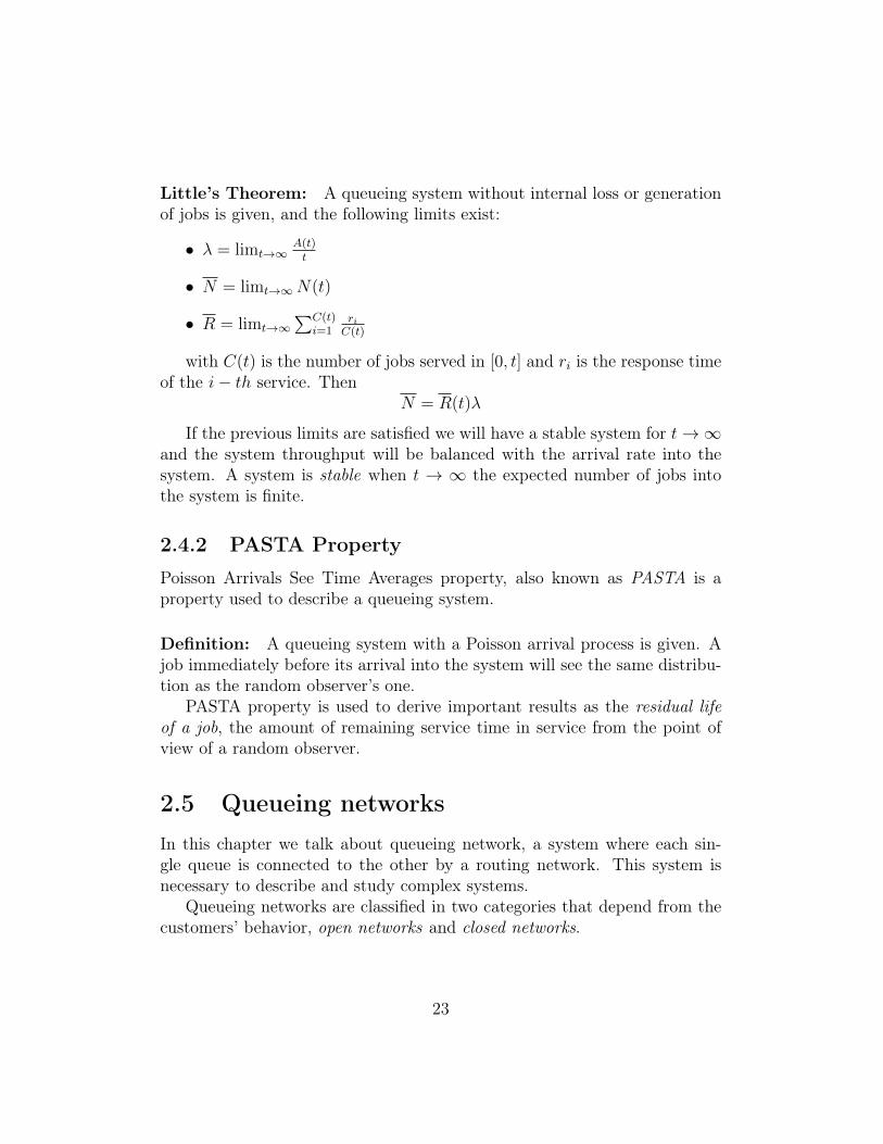
Little’s Theorem: A queueing system without internal loss or generationof jobs is given, and the following limits exist:

• λ = limt→∞A(t)t

• N = limt→∞N(t)

• R = limt→∞∑C(t)

i=1riC(t)

with C(t) is the number of jobs served in [0, t] and ri is the response timeof the i− th service. Then

N = R(t)λ

If the previous limits are satisfied we will have a stable system for t→∞and the system throughput will be balanced with the arrival rate into thesystem. A system is stable when t → ∞ the expected number of jobs intothe system is finite.

2.4.2 PASTA Property

Poisson Arrivals See Time Averages property, also known as PASTA is aproperty used to describe a queueing system.

Definition: A queueing system with a Poisson arrival process is given. Ajob immediately before its arrival into the system will see the same distribu-tion as the random observer’s one.

PASTA property is used to derive important results as the residual lifeof a job, the amount of remaining service time in service from the point ofview of a random observer.

2.5 Queueing networksIn this chapter we talk about queueing network, a system where each sin-gle queue is connected to the other by a routing network. This system isnecessary to describe and study complex systems.

Queueing networks are classified in two categories that depend from thecustomers’ behavior, open networks and closed networks.

23

2.5.1 Open Network

An open network is characterized by one or more input customers streamand one or more output customers stream. We study steady-state behaviorof queueing network. To achieve this goal is necessary to understand andtest when a queueinq network is unstable.

Definition: An open queueing network is defined unstable when the num-ber of jobs into the system go to infinity for t→∞ with higher probability.Let N the expected number of user into the system. If exists the limit

N = limn→∞N(t)

t

the the system will be stable. If a open queueing network is stable, thenall its stations will be stable.

In a stable open queueing network, the total input flow into a stationwill be equal to its throughput. The trough, then, is independent from theservice rates of the stations.

2.5.2 Closed Network

A network can be defined closed if the number of user that interact with thesystem is fixed. Then, there are not arrival and departure to the system.The closed loop networks are classified in two categories: interactive systemsand batch systems. In the interactive system, a customer can pass from athinking state to a submitted state, and from a submitted state to a thinkingstate. The time spent in thinking state is called thinking time (Z). Here thecustomer consumes the obtained result. The time spent in submitted stateis called response time (R). The fixed number of users in the system is alsocalled level of multiprogramming of the system. The combination of thinkingtime and response time allow defining the next definition of system time, sothe time spent from a customer for the entire processing into the system. Toperform it, it is necessary use the expected values.

T = R + Z

We define the response time for an interactive system, emphasizing overthe number of customer into the system, with the following result

24

R(N) =N

X(N)− Z

We can observe that increasing N the response time will increase. Thisbecause there will be more competition into the system. From that relationwe remove the thinking time Z because it does not depend from N but occursin parallel. The response time depends on both level of multiprogrammingand service rates.

We assume that for each station in the network the job service timeis independent from the number of visits for each of them. Then, we canintroduce the service demand. Service demand is a index that measures thetotal amount of service that a customer needs to each station for each visitdone to a reference station

Di = Vi1

µ

And, since 1µis the expected service time for each visit, we can write the

next relation that represents the bottleneck law

pi =Xi

µ=X1Viµ

= X1Di

That relates the service demand to the system throughput and the queuesload factors.

The system speed is bounded by the bottleneck. A bottleneck is theslowest component in the system and the higher system bound are limitedfrom it. Finding the slowest component is possible thanks to the relations

X ≤ min(N

D + Z,

1

Db

)

andR ≥ max(D,NDb − Z)

then

D =K∑j=2

Dj

where Db is the bottleneck of the system that is the max Di. So,

(if pb → 1 when N →∞)→ Xb → µb and ∀b Qb, Ub → 1

25

The last metric that we see in this paragraph is the optimal number ofconcurrent user that the system can accept without degrading its responsetime.

Nopt =D + Z

Db

2.6 Performance testingIn this section we talk about performance testing, an important aspect inthe life cycle of real hardware and software architecture. It allows to analyzeand study the system, describing it. Performance test are classified by goalsand architecture:

1. Performance regression testing : aims to check if system performancehas been degraded after some changes in the code.

2. Performance optimization testing : aims to find the best software con-figuration that improves the performance.

3. Performance benchmarking testing : aims to give a performance de-scription to end users.

4. Scalability testing : aims to find the maximum number of simultaneoususers into the system before performance degradation.

To measure automatically the performance of a system it is necessarythat the employed software simulates the user behavior. Here we distinct thetwo main components: System under test (SUT) and the software that aimsto study its performance, the benchmark. We classify the benchmarks in twocategories:

• Competitive benchmark is a standardized test that aims to assess thesoftware and hardware performance. In this way we can perform con-sistent tests to compare machines or applications.

• Research benchmark is a tool developed to measure the performance ofa certain system. Using this kind of application aims to improve thesoftware performance after and during development time.

We can also split the performance test in four categories:

26

• Synthetic: aims to produce fictitious workload to simulate real cus-tomer behavior.

• Micro: aims to test only one aspect of SUT, without considering therest of application.

• Kernel : aims to test performance from the most important part of theentire application.

• Application: aims to test each single feature of the under analysis ap-plication.

2.7 Statistical inferenceIn this section we talk about the background necessary to understand howand why we have used statistical inference methods to assess the performance[3]. Statistical inference is a process that aims to deduce properties using dataanalysis of a probability distribution. Inferential statistical analysis infersproperties of a population, using a large sample from the population, forexample by testing hypotheses. In this document we decided to use statisticalinference methods to estimate the expected value of AdaORM execution andsimple JDBC execution, assessing the performance improvements in termsof execution time. First of all, we introduce now for the next paragraph twoimportant contents, estimator and hypothesis testing.

Estimator: is an approximation Θ̂ of a distribution parameter Θ per-formed using a sample of the total population. An estimator tries to approx-imate the real value of a population parameter. It’s value is called estimate.

2.7.1 Hypothesis Testing

Hypothesis testing is statistical inference method used to verify statements,claims, conjecture or in general, hypothesis. Hypothesis testing is wide dif-fused in computer science to verify the efficiency of a new algorithm or ahardware upgrade. First of all, we must define what we want to test. Wecall them null hypothesis H0 and alternative hypothesis HA. H0 and HA aremutually exclusive. The rejection of H0 means that we must accept HA. The

27

not rejection of H0 means that we cannot accept HA. To reject H0 in favorof HA is possible only with significant evidence provided by data.

We can describe three different cases for alternative hypothesis HA: two-side alternative, left-side alternative and right-side alternative hypothesis.

two-side alternative H0 : Θ = Θ̂ HA : Θ 6= Θ̂

left-side alternative H0 : Θ < Θ̂ HA : Θ ≥ Θ̂

right-side alternative H0 : Θ > Θ̂ HA : Θ ≤ Θ̂

Table 2.2: Recap of different type of alternative hypothesis

Performing an hypothesis test could make some mistakes. Type I erroroccurs when we reject the true null hypothesis, Type II error occurs when weaccept a false null hypothesis. The type I error is the most dangerous andwe want to avoid it absolutely. We assign a probability to commit this error,called significance level α of a test.

α = P (reject H0 | H0 is true)

Hypothesis test is based on test statistic T. Then, to test our estimatorwe must first of all normalize the value

TΘ̂ =Θ̂−Θ0

SE(Θ̂)

Figure 2.4: Acceptance and rejection regions

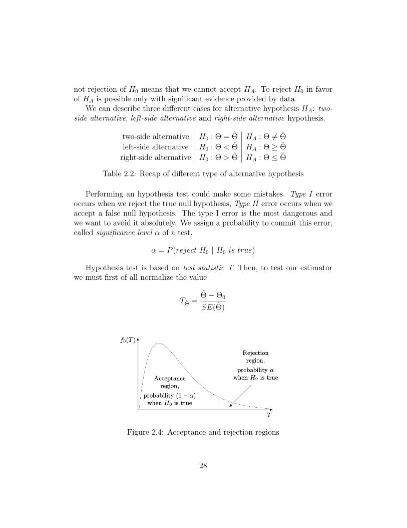
28

Using T statistic we are assessing that we are using null distribution.Then, we split the distribution in two areas acceptance region with probability(1 − α) when H0 is true and rejection region α when H0 is true. Rejectionregions are the tail (or the tails in two-side alternative) of the null distribution(in Figure 2.41 we can see a right tail of the null distribution).

Supposing that the estimator Θ̂ is unbiased and normally distributed, thenull hypothesis can be tested usingZ-statistic

Z =Θ̂−Θ0

SE(Θ̂)

that has a normal null distribution. When Θ̂ is consistent and asymptot-ically normal, if the sample size is large enough Z has approximate standardnormal distribution under the null.

We interpret Z values in the following manner{close to zero→ insufficient evidence against H0

far to zero→ evidence against H0

According to three alternative seen before, now we explain how interpret-ing z − statistics

Right-tail alternative

H0 : Θ = θ0 vs HA : Θ > Θ0

The rejection region R consists of ’large values’ of Z:

R = [zα,+∞) and A = (−∞, zα)

Significance level:

Pr(Type we error) = Pr(Z ∈ R|H0)

= Pr(Z > zα)

= α

(2.1)

1Figure from [3]

29

Left-tail alternative

H0 : Θ = θ0 vs HA : Θ < Θ0

The rejection region R consists of ’small values’ of Z:

R = (−∞,−zα) and A = [−zα,+∞)

Significance level:

Pr(Type we error) = Pr(Z ∈ R|H0)

= Pr(Z < −zα)

= α

(2.2)

Two-side alternative

H0 : Θ = θ0 vs HA : Θ 6= Θ0

The rejection region R consists of ’large’ and ’small’ values of Z:

R = (−∞,−zα/2) ∪ [zα/2,+∞) and A = (−z∞/2, zα/2)

Significance level:

Pr(Type we error) = Pr(Z ∈ R|H0)

= Pr(Z < −zα/2Pr(Z > zα/2)

=α

2+α

2= α

(2.3)

In this chapter we have covered the main topics to provide a sufficientbackground for the complete understanding of the following chapters. Weexplained what a database is and what a DBMS is. We have seen the differ-ences between relational and non-relational DBMS. So, we have seen someof the main patterns that we have implemented describing the problem theyaim and how they solve it. Then, we have given an introduction to the multi-tier architecture of computer systems. We provided the knowledge necessaryto understand the theory of queues and we motivated the need to apply per-formance tests. Finally, we have described the statistical method used toaffirm the improvement in response times. Now, we are ready to move on tothe next chapters.

30

Chapter 3

Implementation of AdaORM

In this chapter, we explain what technologies we used to develop AdaORM andwhy we chose them. We talk about the programming languages, frameworks,libraries, patterns and their integration in the project. Then, we explain themost interesting parts and we give an explanation of the three main cores ofthe system.

3.1 Software

3.1.1 Programming language

AdaORM has been implemented using Java 8 programming language. We chosethis language with this version because it is enough evolved and diffused,that it has given us the opportunity to have access to many libraries thatcan improve my work. Also, some features as lambda functions aren’tavailable in previous versions.

3.1.2 Database

Choosing the correct DBMS according to the case can improve the systemperformance. In our case of study the choice of DBMS is fundamental. Todevelop AdaORM we have chosen as host DBMS, the DBMS that stores infor-mation that we want to fetch, IBM DB2[10] because, as we can see in nextchapter, it implements a mandatory feature that we exploited to achieve ourgoals.

31

However, AdaORM uses two DBMS, the first is the host database, IBM DB2,the second is the system database, SQLitethat contains the collected execu-tion statistics. We chose to use SQLitebecause the database is not sharedexternally with any other process and using a database on the network wouldhave led to problems due to network latency. Furthermore, it is preferablethat the statistics are calculated in the application server in order not to loadthe database server.

3.1.3 Frameworks

A framework is a platform to develop software application. A frameworkprovides an essential behavior that developers can exploit to build specificsoftware. We have used Spring-boot to create an efficient and convenientweb server to expose API. API is used from a client to start routines thatload data from database, according to specific behavior. In this way, we canuse Tsung tool to benchmark AdaORM .

3.1.4 Libraries

Using libraries to develop an application is the best solution. Using thelibraries allows to decrease the development time, it makes the system mod-ular, debuggable and safe. Libraries can also provide essential functions forthe integration of some components such as a DBMS. These are the librariesused in the project

1. sqlite-jdbc version 3.30.1 allows us to interact with SQLitedatabase,our system database.

2. sqlparser version 3.1 implements methods to parse a SQL state-ment. [20].

3. db2jcc version 4.0 allows connection among AdaORM and IBM DB2database, our host database.

4. All mandatory libraries to allow Spring-Boot to work.

3.1.5 Patterns

A pattern is a standard solution to a recurrent problem. Pattern helps im-proving application architecture. The application of these working methods

32

avoids needless bugs and problems. To design a good application we decideto use the following patterns.

Singleton: we made many singleton class. This pattern is very useful tostore data as personal user queries, or to develop some tool class that storesstatus that must be shared uniquely. Also, using singleton instead of staticclasses allow to implement interfaces. Implementing interfaces are a keyfeature to improve code reusability and to decrease coupling.

DAO: Submitting database queries is possible thanks to the use of DataAccess Object (DAO). We made this choice to centralize requests for eachdatabase. Also, we used a customized version of this pattern. In fact, weexploits the fact that each class that wants to use the prediction featuresmust implement an interface. In this way, we are able to generalize objectcreation, asking to the user only to override two particular methods:

• makeBean(ResultSet rs) → T

• getQuery() → String

Implementing these two functions the user teaches to the system howto get the correct kind of object with the correct query. The DAO that weimplement exploits two main functionality: generalization and dynamic cast-ing. Each POJO must be extended by a decorator that implements interfaceDBPredicted. In this way, DAO is able to work with this type of object, call-ing getParameters() → SmartMap a methods that return a Map that hasas key a string that represents the name of POJO property, and as value awrapper that contains all information about the loading and storing methodsto interact with the POJO property.

Strategy with lambdas: is a pattern used to split algorithm from data.In this way, we can reach the aim to develop classes with single responsibilityand improve code reusability. However, for our purpose, it is not enough.We decided to use this pattern combined with lambda functions to modelthe getting procedures of a property in a class. When we load objects, itcould happen that to improve performance, the application doesn’t load allproperties values. Then, to get the next requested values but not loaded,is necessary to develop a procedure that allows us to do it. This procedure

33

follows always the same procedure, but changes the applied functions that getand set object properties (in fact depend from which properties we want tofetch). To solve this problem, we have a main algorithm inside the class, andas parameters we pass getting and setting object methods. So, writing only ageneral class we can define the properties fetching method for all parametersthat respect our constraints.

Factory: Factory pattern centralizes object creation. We exploit featuresof factory and DAO patterns to generalize object instance. The factorycentralize methods to allow creation of collections of items. A method wrapsa generic abstract DAO that requires the implementation of two methods:

• makeBean() → DBPredicted

• getQuery() → QuerySmart

makeBean() requires to be implemented so that it returns the item typethat must be stored into the required collection. getQuery() requires to beimplemented so that it returns a QuerySmart, a wrapper that contains SQLinformation to fetch collection from DB.

Decorator: Decorator plays a very important role in AdaORM design, be-cause it allows to reduce inheritance explosion and adapt the functionalityand data of an existing POJO to a new object that contains methods to talkwith the system, without changing too many lines of the code in a (possible)existing project.

3.1.6 Main functionalities

We can split AdaORM into three main cores:

1. Object mapping and recording

2. Statistic computation

3. Query prediction

Now we explain all the three parts.

34

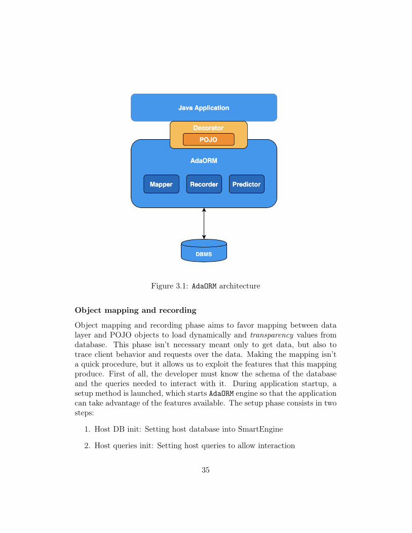
Figure 3.1: AdaORM architecture

Object mapping and recording

Object mapping and recording phase aims to favor mapping between datalayer and POJO objects to load dynamically and transparency values fromdatabase. This phase isn’t necessary meant only to get data, but also totrace client behavior and requests over the data. Making the mapping isn’ta quick procedure, but it allows us to exploit the features that this mappingproduce. First of all, the developer must know the schema of the databaseand the queries needed to interact with it. During application startup, asetup method is launched, which starts AdaORM engine so that the applicationcan take advantage of the features available. The setup phase consists in twosteps:

1. Host DB init: Setting host database into SmartEngine

2. Host queries init: Setting host queries to allow interaction

35

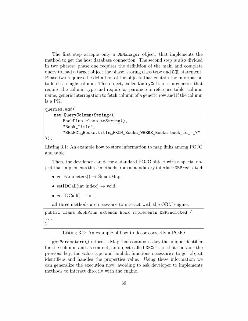
The first step accepts only a DBManager object, that implements themethod to get the host database connection. The second step is also dividedin two phases: phase one requires the definition of the main and completequery to load a target object the phase, storing class type and SQL statement.Phase two requires the definition of the objects that contain the informationto fetch a single column. This object, called QueryColumn is a generics thatrequire the column type and require as parameters reference table, columnname, generic interrogation to fetch column of a generic row and if the columnis a PK.

queries.add(new QueryColumn<String>(

BookPlus.class.toString(),"Book_Title","SELECT␣Books.title␣FROM␣Books␣WHERE␣Books.book_id␣=␣?"

));

Listing 3.1: An example how to store information to map links among POJOand table

Then, the developer can decor a standard POJO object with a special ob-ject that implements three methods from a mandatory interface DBPredicted:

• getParameters() → SmartMap;

• setIDCall(int index) → void;

• getIDCall() → int;

all three methods are necessary to interact with the ORM engine.

public class BookPlus extends Book implements DBPredicted {...}

Listing 3.2: An example of how to decor correctly a POJO

getParameters() returns a Map that contains as key the unique identifierfor the column, and as content, an object called DBColumn that contains theprevious key, the value type and lambda functions necessaries to get objectidentifiers and handles the properties value. Using these information wecan generalize the execution flow, avoiding to ask developer to implementsmethods to interact directly with the engine.

36

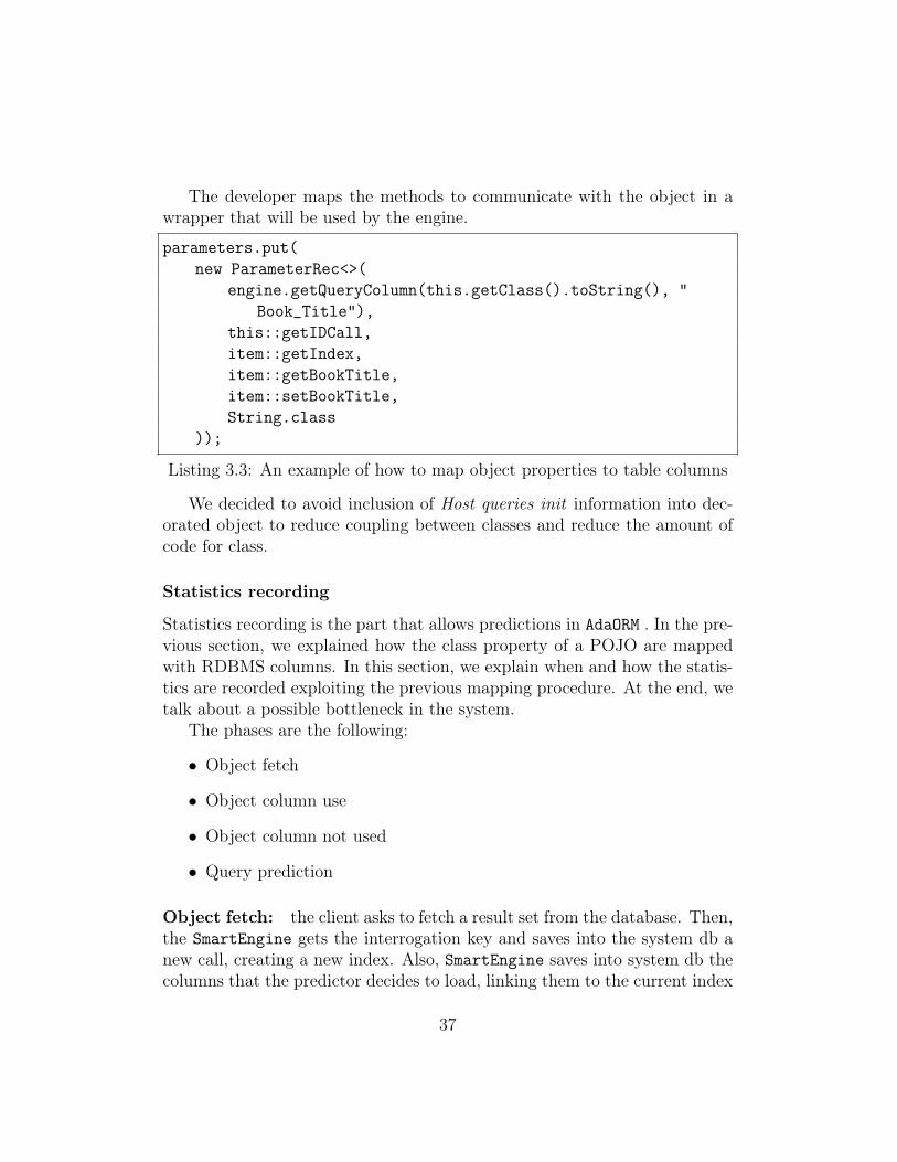
The developer maps the methods to communicate with the object in awrapper that will be used by the engine.

parameters.put(new ParameterRec<>(

engine.getQueryColumn(this.getClass().toString(), "Book_Title"),

this::getIDCall,item::getIndex,item::getBookTitle,item::setBookTitle,String.class

));

Listing 3.3: An example of how to map object properties to table columns

We decided to avoid inclusion of Host queries init information into dec-orated object to reduce coupling between classes and reduce the amount ofcode for class.

Statistics recording

Statistics recording is the part that allows predictions in AdaORM . In the pre-vious section, we explained how the class property of a POJO are mappedwith RDBMS columns. In this section, we explain when and how the statis-tics are recorded exploiting the previous mapping procedure. At the end, wetalk about a possible bottleneck in the system.

The phases are the following:

• Object fetch

• Object column use

• Object column not used

• Query prediction

Object fetch: the client asks to fetch a result set from the database. Then,the SmartEngine gets the interrogation key and saves into the system db anew call, creating a new index. Also, SmartEngine saves into system db thecolumns that the predictor decides to load, linking them to the current index

37

query call. At the end, the query call index ia set into all fetched items. Inthis way we can memorize the purpose of the query and then increment theutilization of the right column.

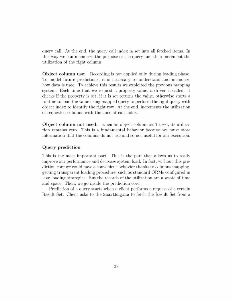
Object column use: Recording is not applied only during loading phase.To model future predictions, it is necessary to understand and memorizehow data is used. To achieve this results we exploited the previous mappingsystem. Each time that we request a property value, a driver is called: itchecks if the property is set, if it is set returns the value, otherwise starts aroutine to load the value using mapped query to perform the right query withobject index to identify the right row. At the end, increments the utilizationof requested columns with the current call index.

Object column not used: when an object column isn’t used, its utiliza-tion remains zero. This is a fundamental behavior because we must storeinformation that the columns do not use and so not useful for our execution.

Query prediction

This is the most important part. This is the part that allows us to reallyimprove our performance and decrease system load. In fact, without this pre-diction core we could have a convenient behavior thanks to columns mapping,getting transparent loading procedure, such as standard ORMs configured inlazy loading strategies. But the records of the utilization are a waste of timeand space. Then, we go inside the prediction core.

Prediction of a query starts when a client performs a request of a certainResult Set. Client asks to the SmartEngine to fetch the Result Set from a

38

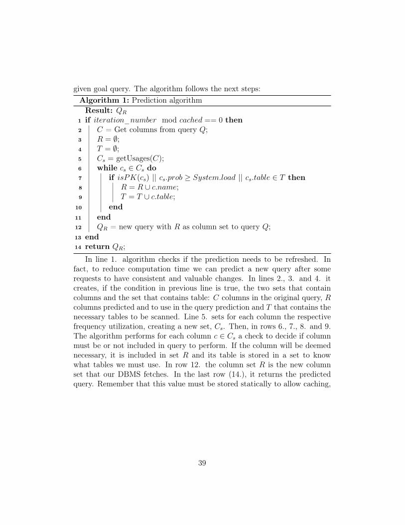
given goal query. The algorithm follows the next steps:Algorithm 1: Prediction algorithmResult: QR

1 if iteration_number mod cached == 0 then2 C = Get columns from query Q;3 R = ∅;4 T = ∅;5 Cs = getUsages(C);6 while cs ∈ Cs do7 if isPK(cs) || cs.prob ≥ System.load || cs.table ∈ T then8 R = R ∪ c.name;9 T = T ∪ c.table;

10 end11 end12 QR = new query with R as column set to query Q;13 end14 return QR;

In line 1. algorithm checks if the prediction needs to be refreshed. Infact, to reduce computation time we can predict a new query after somerequests to have consistent and valuable changes. In lines 2., 3. and 4. itcreates, if the condition in previous line is true, the two sets that containcolumns and the set that contains table: C columns in the original query, Rcolumns predicted and to use in the query prediction and T that contains thenecessary tables to be scanned. Line 5. sets for each column the respectivefrequency utilization, creating a new set, Cs. Then, in rows 6., 7., 8. and 9.The algorithm performs for each column c ∈ Cs a check to decide if columnmust be or not included in query to perform. If the column will be deemednecessary, it is included in set R and its table is stored in a set to knowwhat tables we must use. In row 12. the column set R is the new columnset that our DBMS fetches. In the last row (14.), it returns the predictedquery. Remember that this value must be stored statically to allow caching,

39

avoiding useless computation.Algorithm 2: Algorithm to get frequenciesResult: Cs

1 Cs = ∅;2 while c ∈ C do3 frequency = getFrequency(c);4 Cs = Cs ∪ (c, frequency);5 end6 return Cs;

In line 1. We create a new data structure where we store our result. In line2. the while loop where for each column we want to get its frequency starts.Line 3. performs a database call that fetches from view into the database thealready performed frequency. In the next step we save the column and itsfrequency into the Cs map. In the last step returns the data structure filled.We have used a view to maintain always updated the columns frequencies.In this way, when we want to fetch the requested values we have not executea complex and expensive query, but we retrieve information faster becausethey are already computed.

Complexity: the complexity of the prediction algorithm depends from thenumber of columns that the submitted query has. In fact, to get columnfrequencies the methods complexity is Θ(|C|) and to check which columnsload has a complexity always of Θ(|CS|) = Θ(|C|). Then we can concludethat the asymptotic complexity of AdaORM prediction algorithm is

Θ(|C|+ |C|) = Θ(2|C|) = Θ(|C|)

3.1.7 Conclusion

In this chapter we have seen how AdaORM has been developed. We have talkedabout databases, frameworks, libraries choice. We explained because we usedsome pattern and how they are integrated in AdaORM . Then, we have seenhighlights code parts, for example how to write a POJO compatible withAdaORM and how to perform communication among decorated POJOs andsystem engine. At the end, we have shown prediction algorithm and we havetalked about its complexity.

40

Chapter 4

Experiments and Analysis ofAdaORM

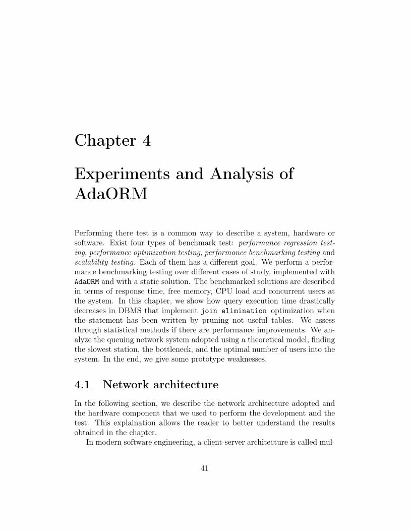
Performing there test is a common way to describe a system, hardware orsoftware. Exist four types of benchmark test: performance regression test-ing, performance optimization testing, performance benchmarking testing andscalability testing. Each of them has a different goal. We perform a perfor-mance benchmarking testing over different cases of study, implemented withAdaORM and with a static solution. The benchmarked solutions are describedin terms of response time, free memory, CPU load and concurrent users atthe system. In this chapter, we show how query execution time drasticallydecreases in DBMS that implement join elimination optimization whenthe statement has been written by pruning not useful tables. We assessthrough statistical methods if there are performance improvements. We an-alyze the queuing network system adopted using a theoretical model, findingthe slowest station, the bottleneck, and the optimal number of users into thesystem. In the end, we give some prototype weaknesses.

4.1 Network architectureIn the following section, we describe the network architecture adopted andthe hardware component that we used to perform the development and thetest. This explaination allows the reader to better understand the resultsobtained in the chapter.

In modern software engineering, a client-server architecture is called mul-

41

titier architecture when the application processing layer and data processingare physically split.

The developing and testing of AdaORM is based on this architecture thatis commonly adopted in a real systems. By this assumption, we are able toperform some interestings test with Tsung benchmark tool that show us howthe system performance changes in a real architecture.

Figure 4.1: Two tier architecture implemented

In figure 4.1 we see how the system architecture has been developed. Theleft-hand panel contains some clients that perform requests to the applicationserver to get results through the call of APIs. The right-hand side panelcontains the developed system: the web server that contains an applicationthat uses AdaORM and sends predicted queries (and column queries to fetchmissing values) to the DB server.

Using this kind of architecture we can study the performance of our sys-tem. In fact, each application/db servers can be replicate many times forreliability or performance reason. In this way, if a node fails, our system cancontinue to work. However, in this thesis we did not focus over this aspect,letting the implementation of the system to developer preference and cases.

4.1.1 Application Server

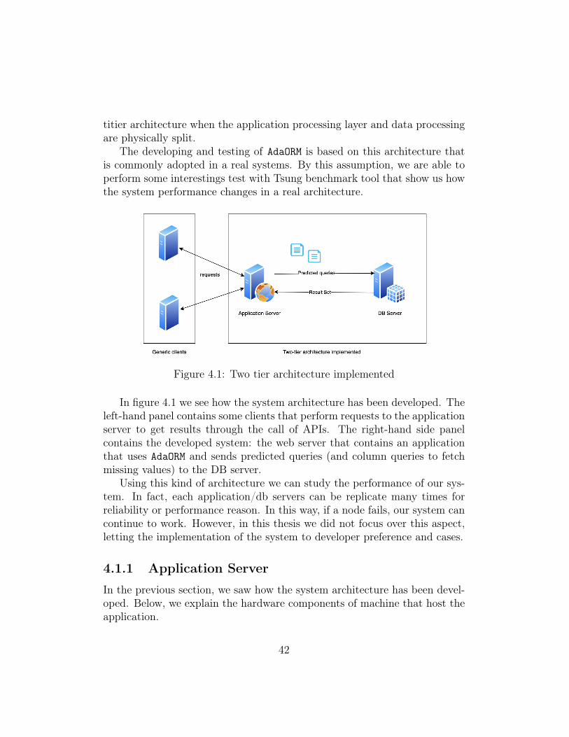
In the previous section, we saw how the system architecture has been devel-oped. Below, we explain the hardware components of machine that host theapplication.

42

Components Characteristic

Device Apple MacBook Pro 13"CPU 2 GHz Dual-Core Intel Core i5 6th generation

Cache L1 32k/32k x2Cache L2/L3 256k x2, 4 MB*

RAM 8 GB 1867 MHz LPDDR3VRAM 1.5 GBGPU -

Secondary memory 250 GB SSDOperative System macOS Catalina 10.15.5 (19F101)

Table 4.1: Developing machine skills

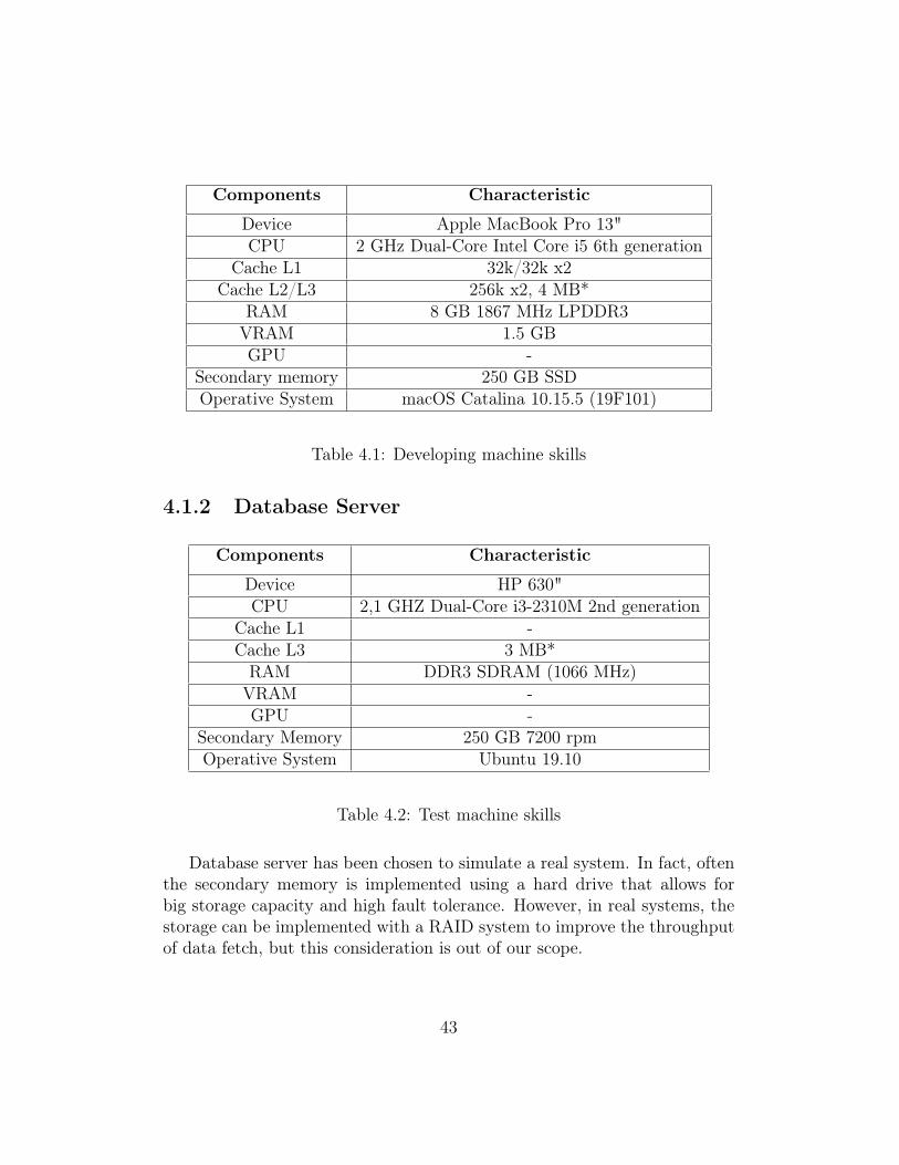
4.1.2 Database Server

Components Characteristic

Device HP 630"CPU 2,1 GHZ Dual-Core i3-2310M 2nd generation

Cache L1 -Cache L3 3 MB*RAM DDR3 SDRAM (1066 MHz)VRAM -GPU -

Secondary Memory 250 GB 7200 rpmOperative System Ubuntu 19.10

Table 4.2: Test machine skills

Database server has been chosen to simulate a real system. In fact, oftenthe secondary memory is implemented using a hard drive that allows forbig storage capacity and high fault tolerance. However, in real systems, thestorage can be implemented with a RAID system to improve the throughputof data fetch, but this consideration is out of our scope.

43

4.2 Databases BenchmarkIn this thesis database benchmark is not a way to assess wich is the fastestDMBS, but a way to study how the presence of join elimination , thefeature that prunes unnecessary joins, can drastically improve performance.First of all, we specify the three kinds of queries that we have performed.

1. Query type #1 (or Heavy query): is an optimized statement that callsat least one parameter for each table that has been requested. Thisquery is the most expensive that we have decided to test.

2. Query type #2 (or Light query): is an optimized which requires to scanonly a table. This is the cheapest query that we have decided to test.

3. Query type #3 (or Critical query): is a statement that calls onlycolumns from the principal table inserted in FROM clause. This is acritical interrogation because, although it calls only columns from asingle table without the needs to join or filter other tables, if the joinelimination optimization is not implemented in DBMS, the execu-tion time is close to that of the heavy query. Instead, if the DBMSimplements this optimization, the execution time of the statement isclose to the light query.

All queries introduce the DISTINCT keyword because if we do not use it theDBMS in any case scans and join all the tables specified in the query. Inthe case of many-to-many relationships, to provide a consistent and correctresult, it will have to calculate the multiplicity relations of each row. Then, weassess that if a DBMS implements the join elimination optimization, theexecution time for a critical query is closed to the execution time required by alight query. Otherwise, the execution time is close to that of the heavy queryif the DBMS does not implement the optimization. The comparison has beendone among different queries over the same data set. We never comparedthe execution time among databases because we are not interested in whatdatabase is the fastest, but we want to test how execution times changeusing the three types of queries described above, with or without the joinelimination optimization. Also, for the moment, we do not talk aboutdatabase size and the number of fetched queries because the experiment isconsistent also without these assumptions.

44

In next sections, we analyze the DBMS benchmarks and EXPLAINEDPLANs, a sequence of operations that the DBMS performs to run a SE-LECT, INSERT, UPDATE or DELETE statement, about three DBMS:MySQL, Postgres and DB2. We want to study how the system responds withdifferent kind of queries, to prove that our handled query does not degradethe system performance.

4.2.1 Join Elimination optimization

The implementation of AdaORM largely exploits the join elimination op-timization. join elimination is an optimization implemented in someDBMS that removes unnecessary JOINs to load the right required resultset. Avoiding operations on not mandatory tables can considerably decreasethe query execution time. AdaORM takes advantage of join elimination todelegate the removal of unnecessary tables in the query that it sends to theDBMS.

4.2.2 MySQL

MySQL is a relational DBMS developed by Oracle. It is a free software,one of the most popular RDBMS. We choose this software as a case studyfollowing some of its main features[11]:

• Client/Server architecture: one of the environments where it is neces-sary to manage a high number of requests and therefore it is necessaryto optimize.

• Diffusion: given the strong diffusion, the experiment becomes interest-ing for a large number of users.

Experiment explanation

We have used the following frameworks to perform the experiment:

• RDBMS: MySQL version 8.0.19

• Benchmark tool: mysqlslap [16]

• Dataset: Sample Employees database [17]

45

mysqlslap: is a diagnostic command line application to simulate client loadto a MySQL server. It allows us to get and report the execution time for eachstatement or stage. Using this technology we are able to get the executiontime of our queries to understand how the system manages the critical query.mysqlslap has been customized with the following options:

• –concurrency=1 calculate service time of a query with one user.

• –iterations=50 set the number of experiment iteration.

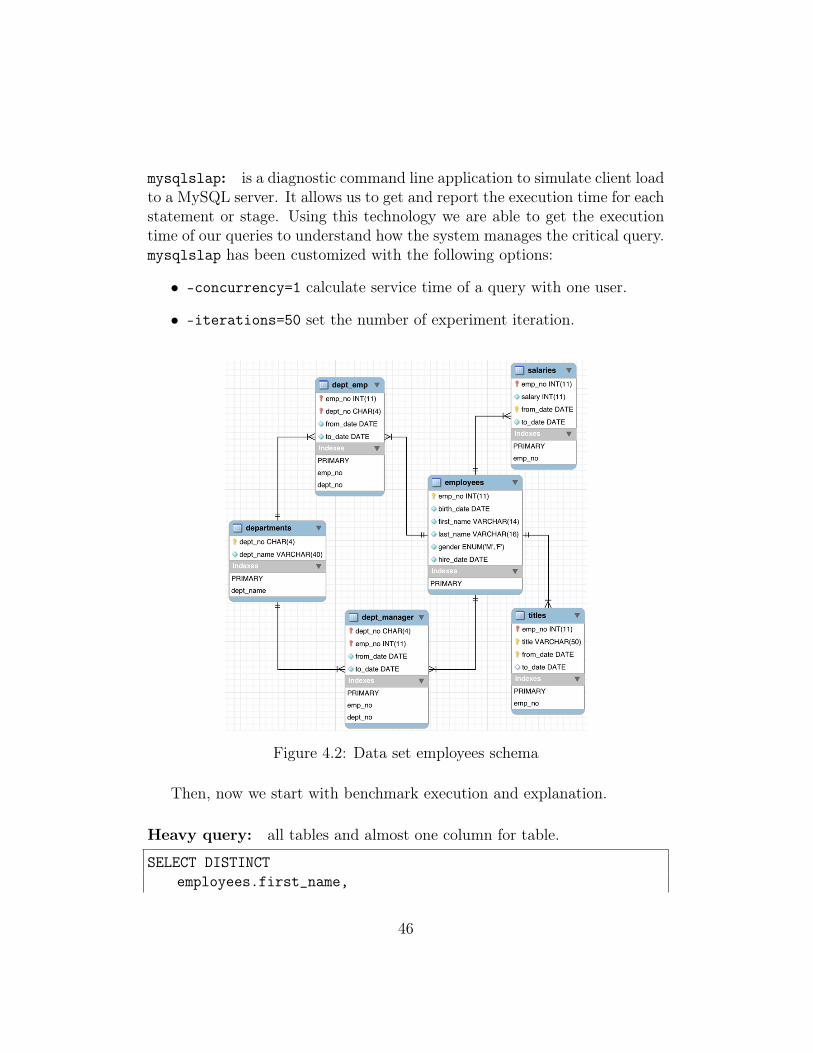
Figure 4.2: Data set employees schema

Then, now we start with benchmark execution and explanation.

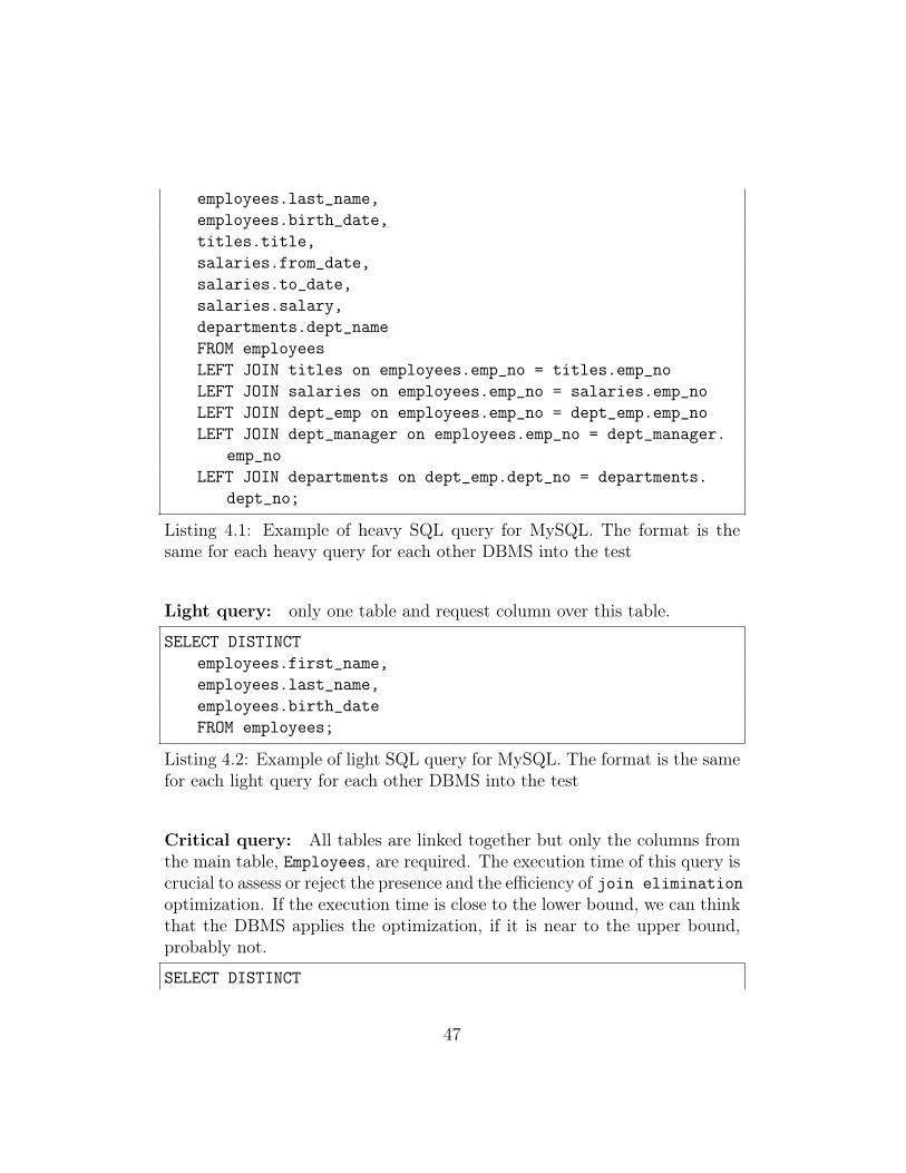
Heavy query: all tables and almost one column for table.

SELECT DISTINCTemployees.first_name,

46

employees.last_name,employees.birth_date,titles.title,salaries.from_date,salaries.to_date,salaries.salary,departments.dept_nameFROM employeesLEFT JOIN titles on employees.emp_no = titles.emp_noLEFT JOIN salaries on employees.emp_no = salaries.emp_noLEFT JOIN dept_emp on employees.emp_no = dept_emp.emp_noLEFT JOIN dept_manager on employees.emp_no = dept_manager.

emp_noLEFT JOIN departments on dept_emp.dept_no = departments.

dept_no;

Listing 4.1: Example of heavy SQL query for MySQL. The format is thesame for each heavy query for each other DBMS into the test

Light query: only one table and request column over this table.

SELECT DISTINCTemployees.first_name,employees.last_name,employees.birth_dateFROM employees;

Listing 4.2: Example of light SQL query for MySQL. The format is the samefor each light query for each other DBMS into the test

Critical query: All tables are linked together but only the columns fromthe main table, Employees, are required. The execution time of this query iscrucial to assess or reject the presence and the efficiency of join eliminationoptimization. If the execution time is close to the lower bound, we can thinkthat the DBMS applies the optimization, if it is near to the upper bound,probably not.

SELECT DISTINCT

47

employees.first_name,employees.last_name,employees.birth_dateFROM employeesLEFT JOIN titles on employees.emp_no = titles.emp_noLEFT JOIN salaries on employees.emp_no = salaries.emp_noLEFT JOIN dept_emp on employees.emp_no = dept_emp.emp_noLEFT JOIN dept_manager on employees.emp_no = dept_manager.

emp_noLEFT JOIN departments on dept_emp.dept_no = departments.

dept_no;

Listing 4.3: Example of critical SQL query for MySQL. The format is thesame for each critical query for each other DBMS into the test

Results

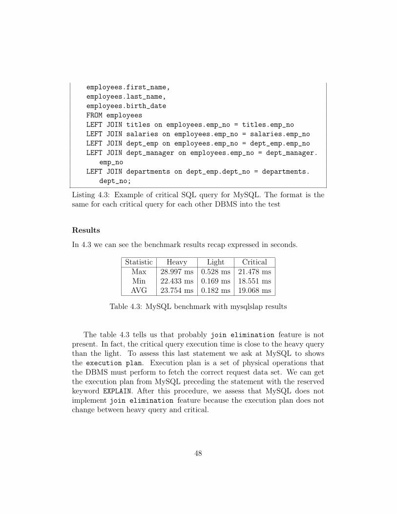
In 4.3 we can see the benchmark results recap expressed in seconds.

Statistic Heavy Light CriticalMax 28.997 ms 0.528 ms 21.478 msMin 22.433 ms 0.169 ms 18.551 msAVG 23.754 ms 0.182 ms 19.068 ms

Table 4.3: MySQL benchmark with mysqlslap results

The table 4.3 tells us that probably join elimination feature is notpresent. In fact, the critical query execution time is close to the heavy querythan the light. To assess this last statement we ask at MySQL to showsthe execution plan. Execution plan is a set of physical operations thatthe DBMS must perform to fetch the correct request data set. We can getthe execution plan from MySQL preceding the statement with the reservedkeyword EXPLAIN. After this procedure, we assess that MySQL does notimplement join elimination feature because the execution plan does notchange between heavy query and critical.

48

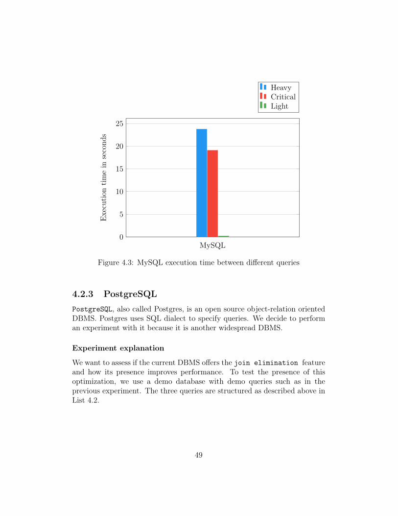
MySQL0

5

10

15

20

25

Execution

timein

second

s

HeavyCriticalLight

Figure 4.3: MySQL execution time between different queries

4.2.3 PostgreSQL

PostgreSQL, also called Postgres, is an open source object-relation orientedDBMS. Postgres uses SQL dialect to specify queries. We decide to performan experiment with it because it is another widespread DBMS.

Experiment explanation

We want to assess if the current DBMS offers the join elimination featureand how its presence improves performance. To test the presence of thisoptimization, we use a demo database with demo queries such as in theprevious experiment. The three queries are structured as described above inList 4.2.

49

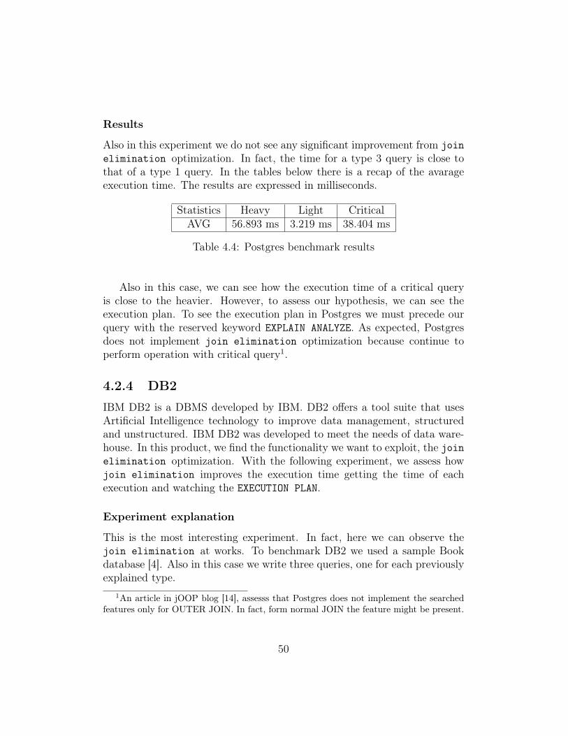
Results

Also in this experiment we do not see any significant improvement from joinelimination optimization. In fact, the time for a type 3 query is close tothat of a type 1 query. In the tables below there is a recap of the avarageexecution time. The results are expressed in milliseconds.

Statistics Heavy Light CriticalAVG 56.893 ms 3.219 ms 38.404 ms

Table 4.4: Postgres benchmark results

Also in this case, we can see how the execution time of a critical queryis close to the heavier. However, to assess our hypothesis, we can see theexecution plan. To see the execution plan in Postgres we must precede ourquery with the reserved keyword EXPLAIN ANALYZE. As expected, Postgresdoes not implement join elimination optimization because continue toperform operation with critical query1.

4.2.4 DB2

IBM DB2 is a DBMS developed by IBM. DB2 offers a tool suite that usesArtificial Intelligence technology to improve data management, structuredand unstructured. IBM DB2 was developed to meet the needs of data ware-house. In this product, we find the functionality we want to exploit, the joinelimination optimization. With the following experiment, we assess howjoin elimination improves the execution time getting the time of eachexecution and watching the EXECUTION PLAN.

Experiment explanation

This is the most interesting experiment. In fact, here we can observe thejoin elimination at works. To benchmark DB2 we used a sample Bookdatabase [4]. Also in this case we write three queries, one for each previouslyexplained type.

1An article in jOOP blog [14], assesss that Postgres does not implement the searchedfeatures only for OUTER JOIN. In fact, form normal JOIN the feature might be present.

50

Postgres0

10

20

30

40

50

60

Execution

timein

ms

HeavyCriticallight

Figure 4.4: PostgreSQL execution time between different queries

IBM provides a command line tool to benchmark the database, db2batch.db2batch can be ran from command line environment setting the follow op-tions (to see the full list, you see the official documentation[8]):

• -d set the database over run the test

• -o set an options

– o set optimization level

– e set

• -q set the query visibility

• -f set the file that contains SQL code to execute

The experiment is performed with the statement db2batch -d demo -o o9 -q del -o e yes -f query.sql

51

The tool that the DB2 production company provides to see the EXECUTIONPLAN is db2expln. Also in this case we have some options to set before ranthe explanation (too read the full documentation see [9]):

• -d set the database over run the test

• -statement set the statement to explain

• -terminal set the terminal as standard output

The explanation is performed with the statement db2expln -d demo-statement "<query>" -terminal

Results

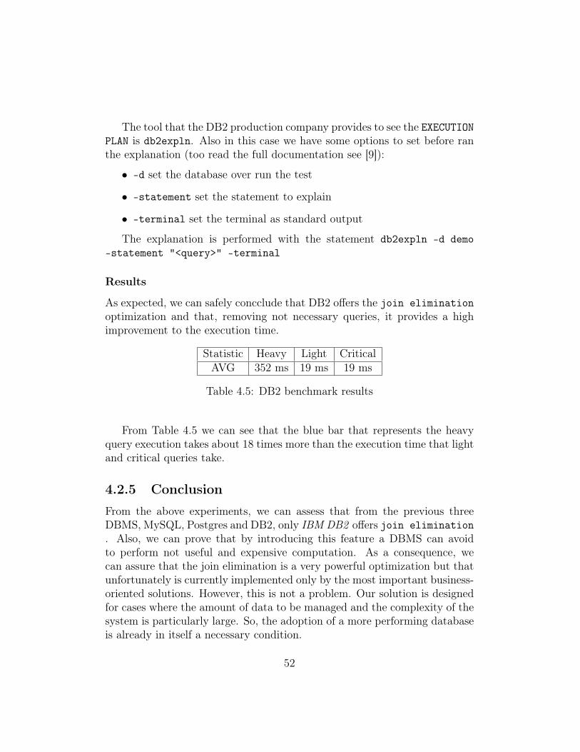
As expected, we can safely concclude that DB2 offers the join eliminationoptimization and that, removing not necessary queries, it provides a highimprovement to the execution time.

Statistic Heavy Light CriticalAVG 352 ms 19 ms 19 ms

Table 4.5: DB2 benchmark results

From Table 4.5 we can see that the blue bar that represents the heavyquery execution takes about 18 times more than the execution time that lightand critical queries take.

4.2.5 Conclusion

From the above experiments, we can assess that from the previous threeDBMS, MySQL, Postgres and DB2, only IBM DB2 offers join elimination. Also, we can prove that by introducing this feature a DBMS can avoidto perform not useful and expensive computation. As a consequence, wecan assure that the join elimination is a very powerful optimization but thatunfortunately is currently implemented only by the most important business-oriented solutions. However, this is not a problem. Our solution is designedfor cases where the amount of data to be managed and the complexity of thesystem is particularly large. So, the adoption of a more performing databaseis already in itself a necessary condition.

52

DB20

0.1

0.2

0.3

Execution

timein

second

s

HeavyCriticalLight

Figure 4.5: DB2 execution time between different queries

4.3 Application BenchmarksIn this section, we explain how we have performed the benchmarks overAdaORM configured with DB2 database. In the first part, we talk about thetest configurations, then we describe the custom benchmark where we havecompared AdaORM with static JDBC solution. In the third part, we showthe plots and the results obtained through the use of Tsung [15] benchmarktool, comparing a web server that uses AdaORM with a web server, with thesame network configuration, that implements a static solution with JDBC.To perform the previous benchmark, we used Spring-Boot to build quickly anefficient and reliable web server, where we write API to interact with DBMS.In the last benchmark that we perform, we compare AdaORM vs HibernateORM tool, showing some results and giving some observations. To assess theconvenience of use AdaORM against a static solution with JDBC or Hibernatewe have used statistic methods hypothesis testing explained in Chapter 2. Inthe last two sections, we explain the queueing network model adopted using

53

the metrics and model introduced in Chapter 2, to conclude giving the limitsof proposed prototype.

4.3.1 Configuration

We include a test package where we implement some demo cases. In thedemo, we write the class to link the host database, we design the POJO thatrepresents the main database item (in this case the Book class). In the end,we write all the queries necessary to fetch the data from database. After weperform this configuration phase, we develop a main class where we simulatefour different cases:

1. (AHQ) Adaptive heavy query

2. (ALQ) Adaptive light query

3. (JHQ) JDBC heavy query

4. (JLQ) JDBC light query

Each case takes its name from the type of query that is performed toload the same goal result set and from the technology used. Then, in eachcase, we want to fetch the same result set but using different strategies. AHQcase applies AdaORM to exploit its features. The case uses a heavier and moreexpensive query, but AdaORM understands, using collected statistics, that notall the columns are useful. So, it predicts a new and lighter query, thatimproves the performance. ALQ applies, also in this case, AdaORM features.Now, it starts using a light query, that loads less data than required. So,it must to fetch in lazy loading missing columns until AdaORM learns, usingcollected statistics, what is the correct dataset to fetch. AHQ and ALQ afterthe wrong prediction, they learn how to predict a faster query and, sincethey want the same result, execution times converge to optimal.

JHQ applies a simple static JDBC connection to fetch a big result setfrom database. Unfortunately, not all fetched columns are useful, but thesystem it is not prepared to manage this case. Then, at each call we havea waste of time and a higher system load. The last case is JLQ that appliesa lighter query, but after the execution, at run-time, it needs to fetch otherinformation, increasing the database requests, execution time and systemload. JHQ and JLQ never converge in analyzed case to optimal solution.They are statically set to load always the same result sets, that are too big

54

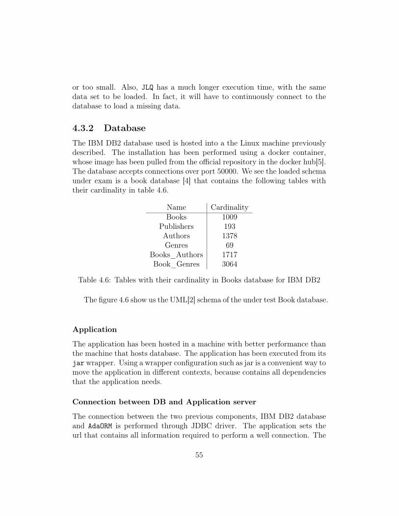
or too small. Also, JLQ has a much longer execution time, with the samedata set to be loaded. In fact, it will have to continuously connect to thedatabase to load a missing data.

4.3.2 Database

The IBM DB2 database used is hosted into a the Linux machine previouslydescribed. The installation has been performed using a docker container,whose image has been pulled from the official repository in the docker hub[5].The database accepts connections over port 50000. We see the loaded schemaunder exam is a book database [4] that contains the following tables withtheir cardinality in table 4.6.

Name CardinalityBooks 1009

Publishers 193Authors 1378Genres 69

Books_Authors 1717Book_Genres 3064

Table 4.6: Tables with their cardinality in Books database for IBM DB2

The figure 4.6 show us the UML[2] schema of the under test Book database.

Application

The application has been hosted in a machine with better performance thanthe machine that hosts database. The application has been executed from itsjar wrapper. Using a wrapper configuration such as jar is a convenient way tomove the application in different contexts, because contains all dependenciesthat the application needs.

Connection between DB and Application server

The connection between the two previous components, IBM DB2 databaseand AdaORM is performed through JDBC driver. The application sets theurl that contains all information required to perform a well connection. The

55

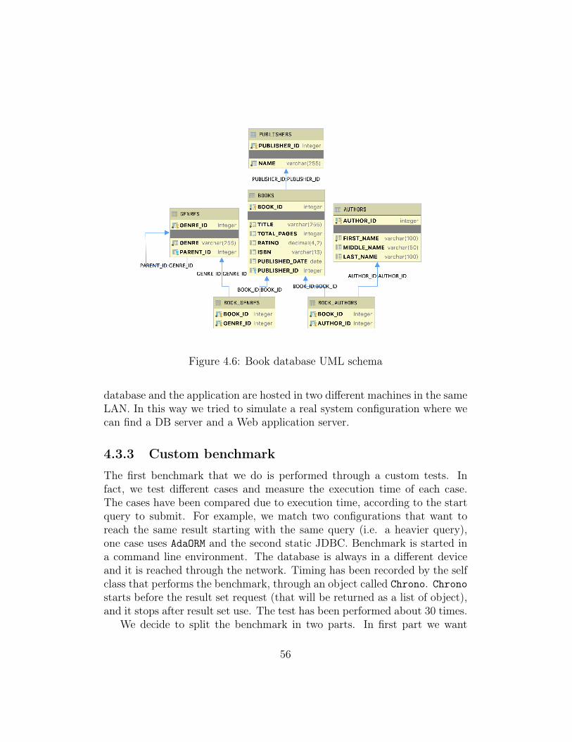
Figure 4.6: Book database UML schema

database and the application are hosted in two different machines in the sameLAN. In this way we tried to simulate a real system configuration where wecan find a DB server and a Web application server.

4.3.3 Custom benchmark

The first benchmark that we do is performed through a custom tests. Infact, we test different cases and measure the execution time of each case.The cases have been compared due to execution time, according to the startquery to submit. For example, we match two configurations that want toreach the same result starting with the same query (i.e. a heavier query),one case uses AdaORM and the second static JDBC. Benchmark is started ina command line environment. The database is always in a different deviceand it is reached through the network. Timing has been recorded by the selfclass that performs the benchmark, through an object called Chrono. Chronostarts before the result set request (that will be returned as a list of object),and it stops after result set use. The test has been performed about 30 times.

We decide to split the benchmark in two parts. In first part we want

56

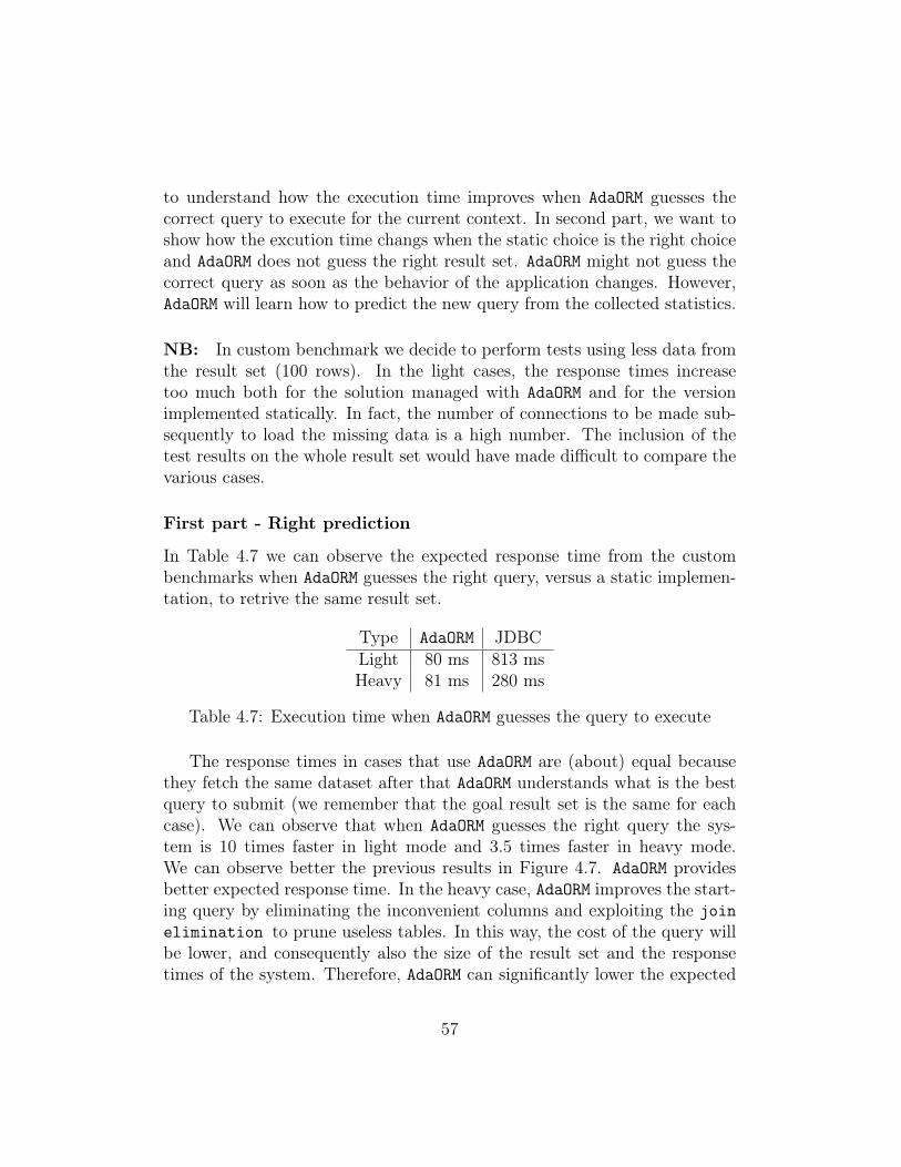
to understand how the execution time improves when AdaORM guesses thecorrect query to execute for the current context. In second part, we want toshow how the excution time changs when the static choice is the right choiceand AdaORM does not guess the right result set. AdaORM might not guess thecorrect query as soon as the behavior of the application changes. However,AdaORM will learn how to predict the new query from the collected statistics.

NB: In custom benchmark we decide to perform tests using less data fromthe result set (100 rows). In the light cases, the response times increasetoo much both for the solution managed with AdaORM and for the versionimplemented statically. In fact, the number of connections to be made sub-sequently to load the missing data is a high number. The inclusion of thetest results on the whole result set would have made difficult to compare thevarious cases.

First part - Right prediction

In Table 4.7 we can observe the expected response time from the custombenchmarks when AdaORM guesses the right query, versus a static implemen-tation, to retrive the same result set.

Type AdaORM JDBCLight 80 ms 813 msHeavy 81 ms 280 ms

Table 4.7: Execution time when AdaORM guesses the query to execute

The response times in cases that use AdaORM are (about) equal becausethey fetch the same dataset after that AdaORM understands what is the bestquery to submit (we remember that the goal result set is the same for eachcase). We can observe that when AdaORM guesses the right query the sys-tem is 10 times faster in light mode and 3.5 times faster in heavy mode.We can observe better the previous results in Figure 4.7. AdaORM providesbetter expected response time. In the heavy case, AdaORM improves the start-ing query by eliminating the inconvenient columns and exploiting the joinelimination to prune useless tables. In this way, the cost of the query willbe lower, and consequently also the size of the result set and the responsetimes of the system. Therefore, AdaORM can significantly lower the expected

57

response time predicting the right query in the light case, which starts ap-pling the lazy strategy. In fact, it will not need to make further connectionsto the database.

Heavy Light0

200

400

600

800

Execution

timein

ms

JDBCAdaORM

Figure 4.7: Home made benchmark comparison - guessed

It is interesting to see how the system works during the first executions.So, in next two-line plot (Figure 4.8 and Figure 4.9), we can see the evolutionof the executions time before AdaORM predicts the right query and after itsprediction.

From Figure 4.8 and Figure 4.9 is evident that the first execution is moreexpensive because the data set to be loaded is the largest, as in the staticchoice. Furthermore, with AdaORM , it is also necessary to carry out operationson the loaded data, which have a cost. However, after few iterations (if theprediction calculation is made at each iteration) AdaORM understands whatis the best query to execute to fetch the right dataset according to the clientbehavior. In the end, at the first execution it is better to run the heavier querybecause, in case we need all the data, we should not make many connectionsto the database. In fact, we can assess from ligh cases that too many database

58

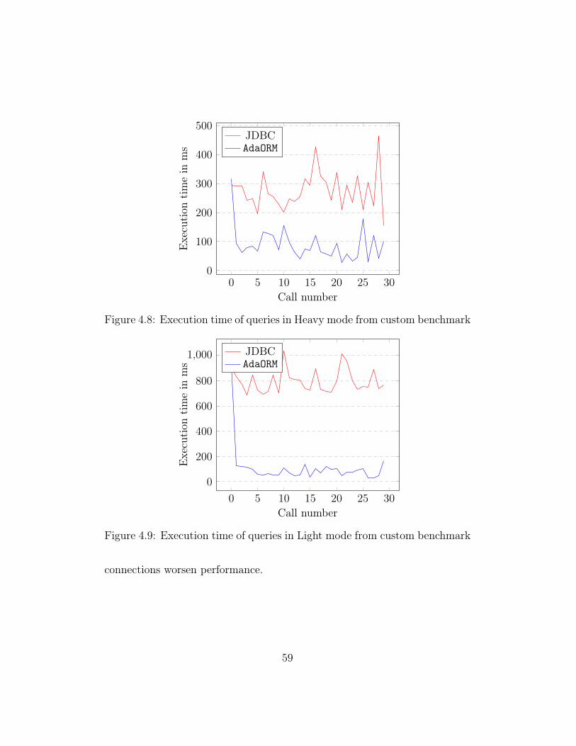
0 5 10 15 20 25 300

100

200

300

400

500

Call number

Execution

timein

ms

JDBCAdaORM

Figure 4.8: Execution time of queries in Heavy mode from custom benchmark

0 5 10 15 20 25 30

0

200

400

600

800

1,000

Call number

Execution

timein

ms

JDBCAdaORM

Figure 4.9: Execution time of queries in Light mode from custom benchmark

connections worsen performance.

59

Second part - Wrong prediction

Now, we analyze the expected response time before AdaORM guesses the rightquery. The guess is wrong because the predictor compute a query with lessparameters and then AdaORMmust load missing data. Notice that, at a certainpoint, the predictor will understand the new application behavior and willcompute the right query.

Type AdaORM JDBCLight 933 ms 813 msHeavy 302 ms 280 ms

Table 4.8: Execution time when AdaORM does not guess the query to execute

Heavy Light0

200

400

600

800

1,000

Execution

timein

ms

JDBCAdaORM

Figure 4.10: Home made benchmark comparison - not guessed

The static cases do not change because, by definition, the query thatwe want to perform is always the same. The most interesting values inthe Table 4.8 are those obtained by AdaORM experiments. This is a very

60

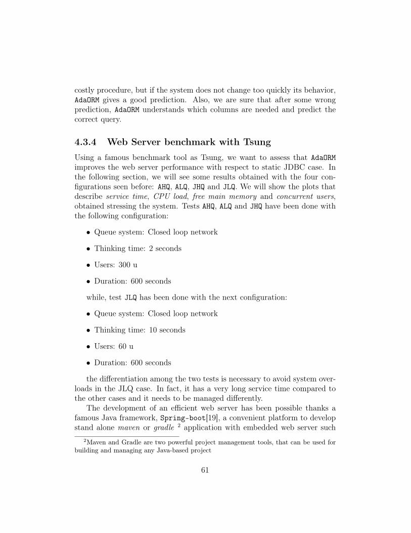
costly procedure, but if the system does not change too quickly its behavior,AdaORM gives a good prediction. Also, we are sure that after some wrongprediction, AdaORM understands which columns are needed and predict thecorrect query.

4.3.4 Web Server benchmark with Tsung

Using a famous benchmark tool as Tsung, we want to assess that AdaORMimproves the web server performance with respect to static JDBC case. Inthe following section, we will see some results obtained with the four con-figurations seen before: AHQ, ALQ, JHQ and JLQ. We will show the plots thatdescribe service time, CPU load, free main memory and concurrent users,obtained stressing the system. Tests AHQ, ALQ and JHQ have been done withthe following configuration:

• Queue system: Closed loop network

• Thinking time: 2 seconds

• Users: 300 u

• Duration: 600 seconds

while, test JLQ has been done with the next configuration:

• Queue system: Closed loop network

• Thinking time: 10 seconds

• Users: 60 u

• Duration: 600 seconds

the differentiation among the two tests is necessary to avoid system over-loads in the JLQ case. In fact, it has a very long service time compared tothe other cases and it needs to be managed differently.

The development of an efficient web server has been possible thanks afamous Java framework, Spring-boot[19], a convenient platform to developstand alone maven or gradle 2 application with embedded web server such

2Maven and Gradle are two powerful project management tools, that can be used forbuilding and managing any Java-based project

61

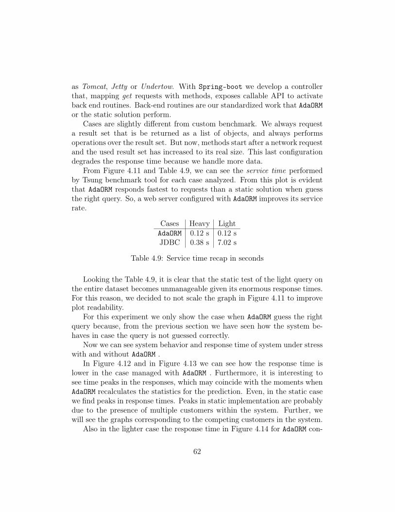
as Tomcat, Jetty or Undertow. With Spring-boot we develop a controllerthat, mapping get requests with methods, exposes callable API to activateback end routines. Back-end routines are our standardized work that AdaORMor the static solution perform.

Cases are slightly different from custom benchmark. We always requesta result set that is be returned as a list of objects, and always performsoperations over the result set. But now, methods start after a network requestand the used result set has increased to its real size. This last configurationdegrades the response time because we handle more data.

From Figure 4.11 and Table 4.9, we can see the service time performedby Tsung benchmark tool for each case analyzed. From this plot is evidentthat AdaORM responds fastest to requests than a static solution when guessthe right query. So, a web server configured with AdaORM improves its servicerate.

Cases Heavy LightAdaORM 0.12 s 0.12 sJDBC 0.38 s 7.02 s

Table 4.9: Service time recap in seconds

Looking the Table 4.9, it is clear that the static test of the light query onthe entire dataset becomes unmanageable given its enormous response times.For this reason, we decided to not scale the graph in Figure 4.11 to improveplot readability.

For this experiment we only show the case when AdaORM guess the rightquery because, from the previous section we have seen how the system be-haves in case the query is not guessed correctly.

Now we can see system behavior and response time of system under stresswith and without AdaORM .

In Figure 4.12 and in Figure 4.13 we can see how the response time islower in the case managed with AdaORM . Furthermore, it is interesting tosee time peaks in the responses, which may coincide with the moments whenAdaORM recalculates the statistics for the prediction. Even, in the static casewe find peaks in response times. Peaks in static implementation are probablydue to the presence of multiple customers within the system. Further, wewill see the graphs corresponding to the competing customers in the system.

Also in the lighter case the response time in Figure 4.14 for AdaORM con-

62

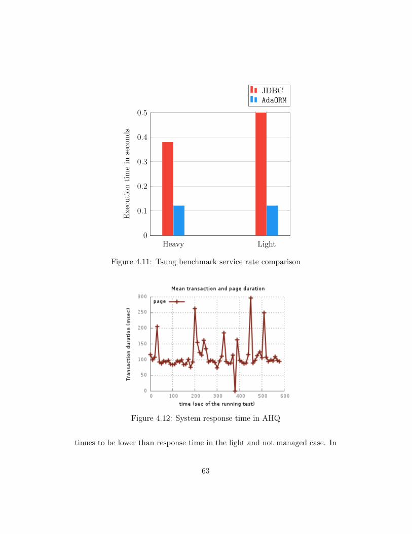
Heavy Light0

0.1

0.2

0.3

0.4

0.5

Execution

timein

second

s

JDBCAdaORM

Figure 4.11: Tsung benchmark service rate comparison

Figure 4.12: System response time in AHQ

tinues to be lower than response time in the light and not managed case. In

63

Figure 4.13: System response time in JHQ

fact, predicting the right result set AdaORM avoids to perform other databaseconnections. Also in this case, peaks in response times are evident, probablydue to the time spent in recalculating the statistics. In Figure 4.15 the situ-ation is slightly different. The peaks in this graph represent a distortion dueto the great expectation in response times.

Figure 4.14: System response time in ALQ

64

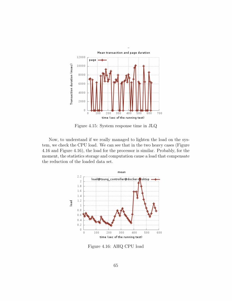
Figure 4.15: System response time in JLQ

Now, to understand if we really managed to lighten the load on the sys-tem, we check the CPU load. We can see that in the two heavy cases (Figure4.16 and Figure 4.16), the load for the processor is similar. Probably, for themoment, the statistics storage and computation cause a load that compensatethe reduction of the loaded data set.

Figure 4.16: AHQ CPU load

65

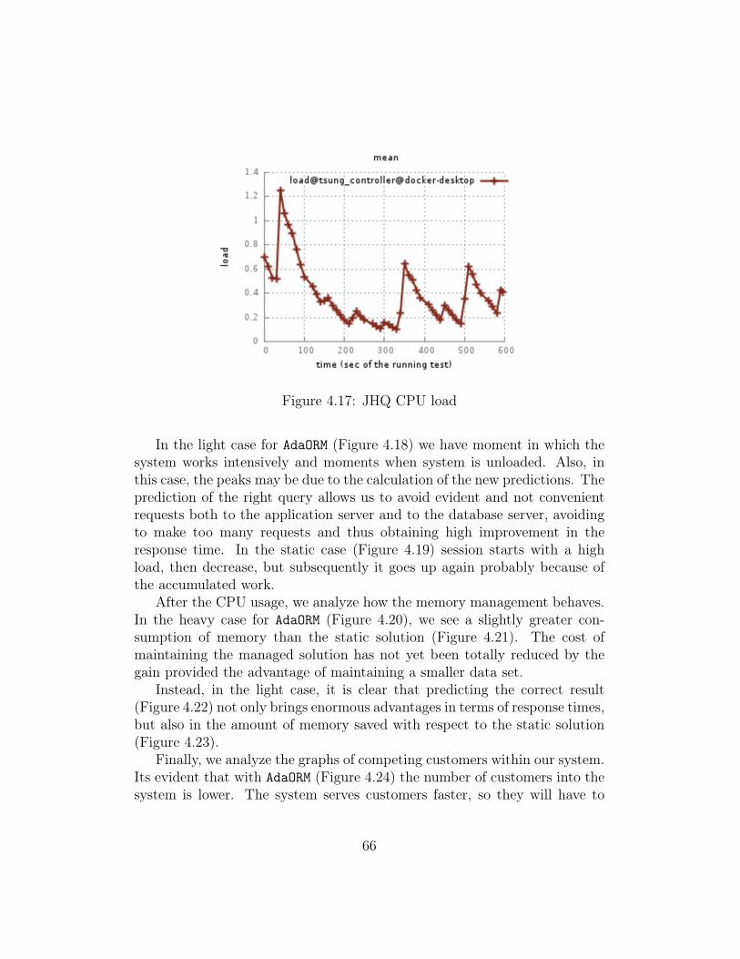
Figure 4.17: JHQ CPU load

In the light case for AdaORM (Figure 4.18) we have moment in which thesystem works intensively and moments when system is unloaded. Also, inthis case, the peaks may be due to the calculation of the new predictions. Theprediction of the right query allows us to avoid evident and not convenientrequests both to the application server and to the database server, avoidingto make too many requests and thus obtaining high improvement in theresponse time. In the static case (Figure 4.19) session starts with a highload, then decrease, but subsequently it goes up again probably because ofthe accumulated work.

After the CPU usage, we analyze how the memory management behaves.In the heavy case for AdaORM (Figure 4.20), we see a slightly greater con-sumption of memory than the static solution (Figure 4.21). The cost ofmaintaining the managed solution has not yet been totally reduced by thegain provided the advantage of maintaining a smaller data set.

Instead, in the light case, it is clear that predicting the correct result(Figure 4.22) not only brings enormous advantages in terms of response times,but also in the amount of memory saved with respect to the static solution(Figure 4.23).

Finally, we analyze the graphs of competing customers within our system.Its evident that with AdaORM (Figure 4.24) the number of customers into thesystem is lower. The system serves customers faster, so they will have to

66

Figure 4.18: ALQ CPU load

Figure 4.19: JLQ CPU load

spend less time within the system by Little’s law.To conclude the plot explanation, we analyze the last test. In the light

cases, a system that uses AdaORM (Figure 4.26, guessing the right query,reduces response times. Then the number of concurrent users into the systemdecreases with respect to the static solution (Figure 4.27).

67

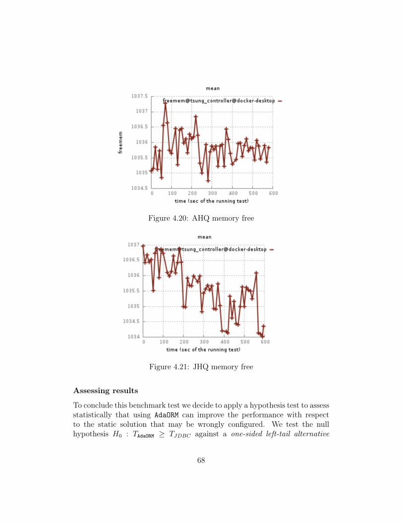
Figure 4.20: AHQ memory free

Figure 4.21: JHQ memory free

Assessing results

To conclude this benchmark test we decide to apply a hypothesis test to assessstatistically that using AdaORM can improve the performance with respectto the static solution that may be wrongly configured. We test the nullhypothesis H0 : TAdaORM ≥ TJDBC against a one-sided left-tail alternative

68

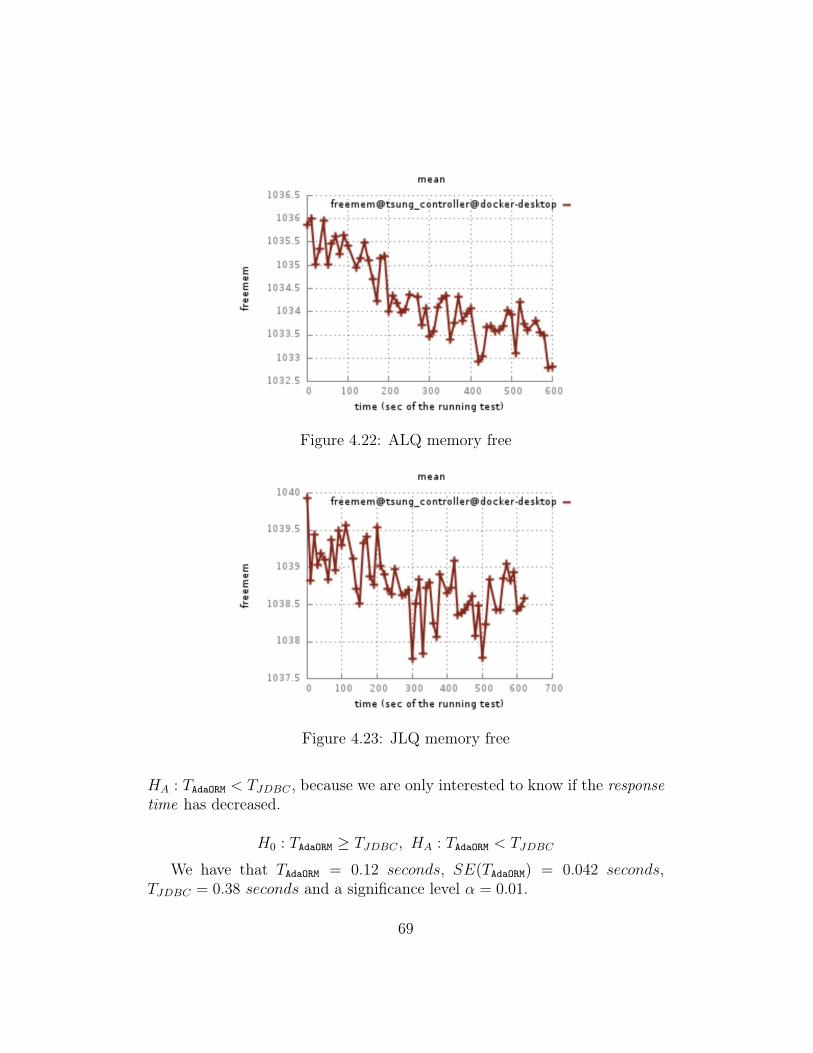
Figure 4.22: ALQ memory free

Figure 4.23: JLQ memory free

HA : TAdaORM < TJDBC , because we are only interested to know if the responsetime has decreased.

H0 : TAdaORM ≥ TJDBC , HA : TAdaORM < TJDBC

We have that TAdaORM = 0.12 seconds, SE(TAdaORM) = 0.042 seconds,TJDBC = 0.38 seconds and a significance level α = 0.01.

69

Figure 4.24: AHQ concurrent users

Figure 4.25: JHQ concurrent users

H0 : TAdaORM ≥ 0.38 s, HA : TAdaORM < 0.38 s

Then we compute the test statistic

Z =TAdaORM − TJDBCSE(TAdaORM)

=0.12− 0.38

0.042= −6.19

70

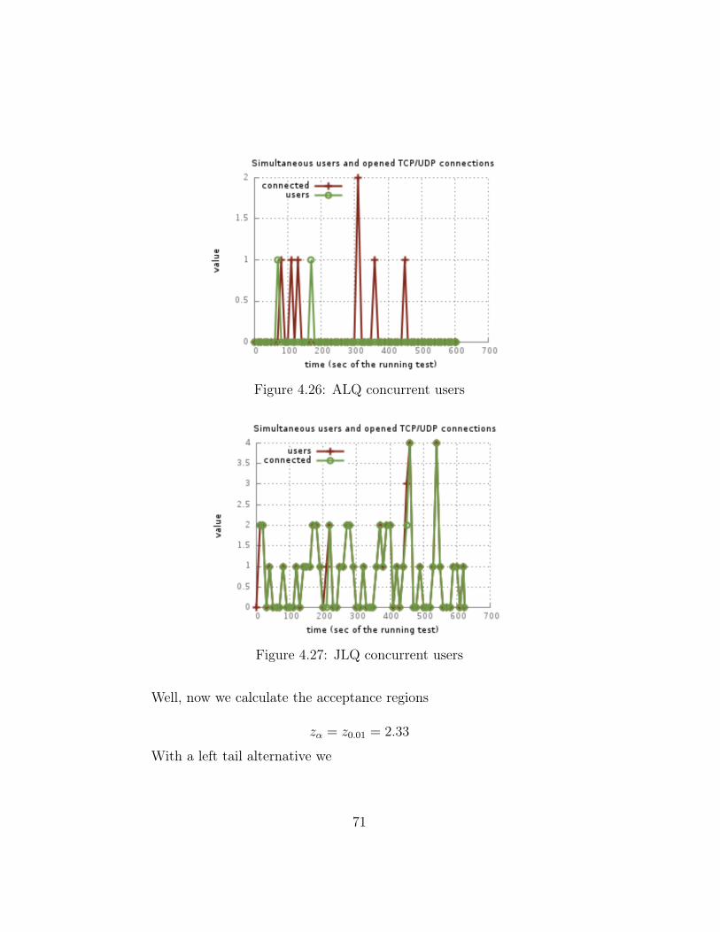
Figure 4.26: ALQ concurrent users

Figure 4.27: JLQ concurrent users

Well, now we calculate the acceptance regions

zα = z0.01 = 2.33

With a left tail alternative we

71

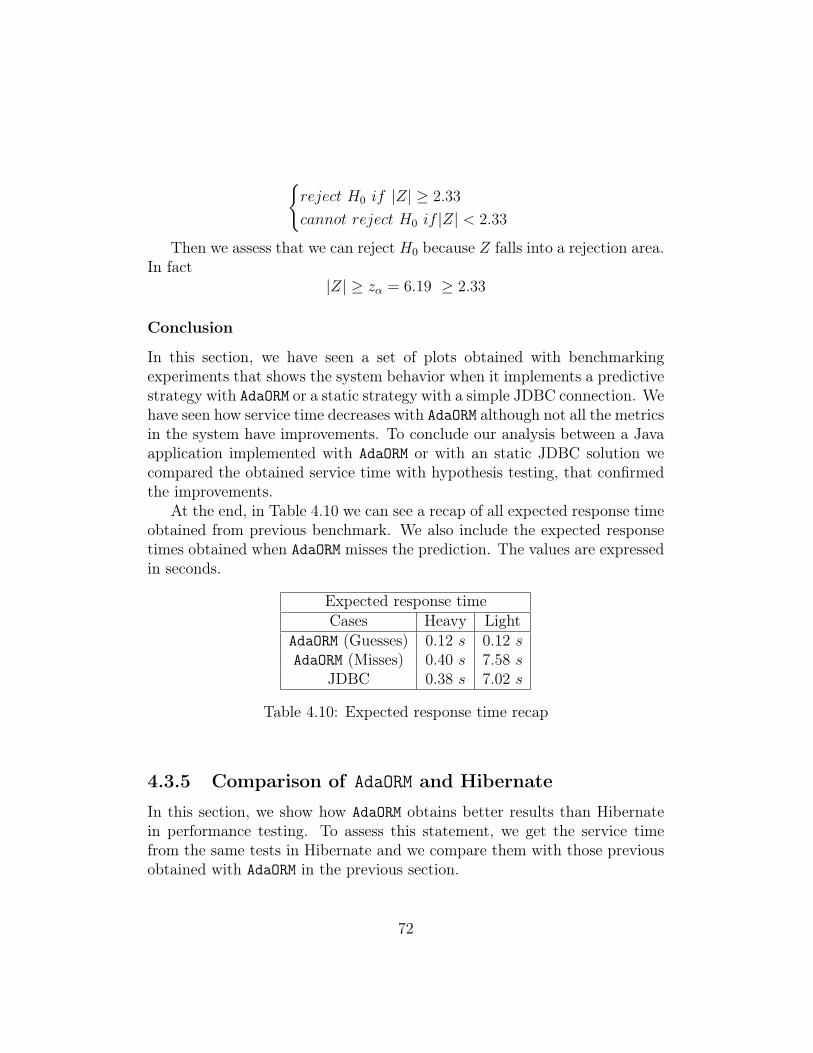
{reject H0 if |Z| ≥ 2.33

cannot reject H0 if |Z| < 2.33

Then we assess that we can reject H0 because Z falls into a rejection area.In fact

|Z| ≥ zα = 6.19 ≥ 2.33

Conclusion

In this section, we have seen a set of plots obtained with benchmarkingexperiments that shows the system behavior when it implements a predictivestrategy with AdaORM or a static strategy with a simple JDBC connection. Wehave seen how service time decreases with AdaORM although not all the metricsin the system have improvements. To conclude our analysis between a Javaapplication implemented with AdaORM or with an static JDBC solution wecompared the obtained service time with hypothesis testing, that confirmedthe improvements.

At the end, in Table 4.10 we can see a recap of all expected response timeobtained from previous benchmark. We also include the expected responsetimes obtained when AdaORM misses the prediction. The values are expressedin seconds.

Expected response timeCases Heavy Light

AdaORM (Guesses) 0.12 s 0.12 sAdaORM (Misses) 0.40 s 7.58 s

JDBC 0.38 s 7.02 s

Table 4.10: Expected response time recap

4.3.5 Comparison of AdaORM and Hibernate

In this section, we show how AdaORM obtains better results than Hibernatein performance testing. To assess this statement, we get the service timefrom the same tests in Hibernate and we compare them with those previousobtained with AdaORM in the previous section.

72

To improve readability of experiments and analysis, we introduce newcases of study for Hibernate:

1. (PR) Prefetching

2. (LL) Light Lazy

3. (LLR) Light Lazy Request

4. (LE) Light Eager

5. (LER) Light Eager Request

Cases of study require the same result set but they apply different strate-gies. Also, we decide to test the cases when we apply request() methods.request() allows the program to load all properties of an object but, howwe will see, it affects performances.

PR: it applies prefetching submitting a heavy query to retrieve all valuesfrom a database. It is equivalent to the static case JHQ seen previously, butimplemented with Hibernate.

LL: it does not apply prefetching and its loading strategy is lazy.

LLR: it does not apply prefetching, its loading strategy is lazy and it appliesthe request() method.

LE: it does not apply prefetching and it uses eager loading strategy. Thisstrategy provides a waste in terms of time and resources if the extra datafetched are not used.

LER: it does not apply prefetching and it uses eager loading strategy andrequest() method to load all data. This strategy provides a large waste oftime and resource if the extra data fetched are not used.

In Table 4.11 we can see at the left-side panel the obtained results fromHibernate benchmarking, at the right-side panel the previously obtained re-sults with AdaORM benchmarking.

From the Figure 4.28 is easy to see that cases in which we ask Hibernate toload all information about a result set, the response times grow exponentially.

73

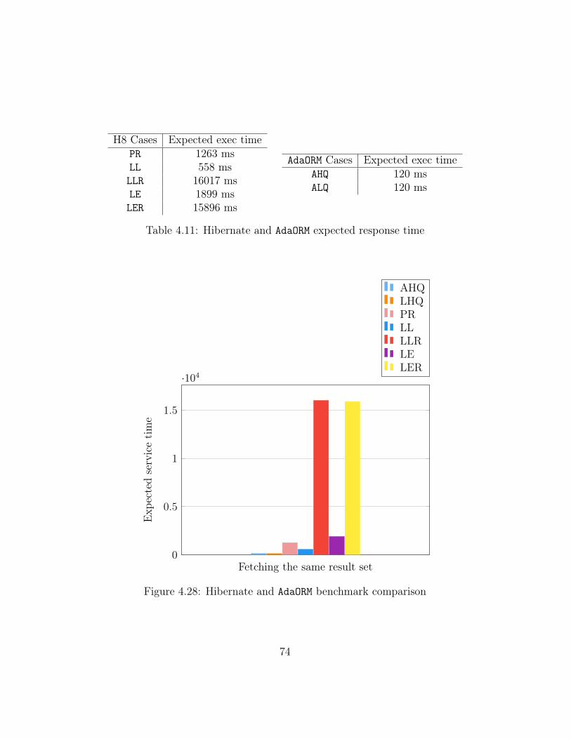
H8 Cases Expected exec timePR 1263 msLL 558 msLLR 16017 msLE 1899 msLER 15896 ms

AdaORM Cases Expected exec timeAHQ 120 msALQ 120 ms

Table 4.11: Hibernate and AdaORM expected response time

Fetching the same result set0

0.5

1

1.5

·104

Exp

ectedservicetime

AHQLHQPRLLLLRLELER

Figure 4.28: Hibernate and AdaORM benchmark comparison

74

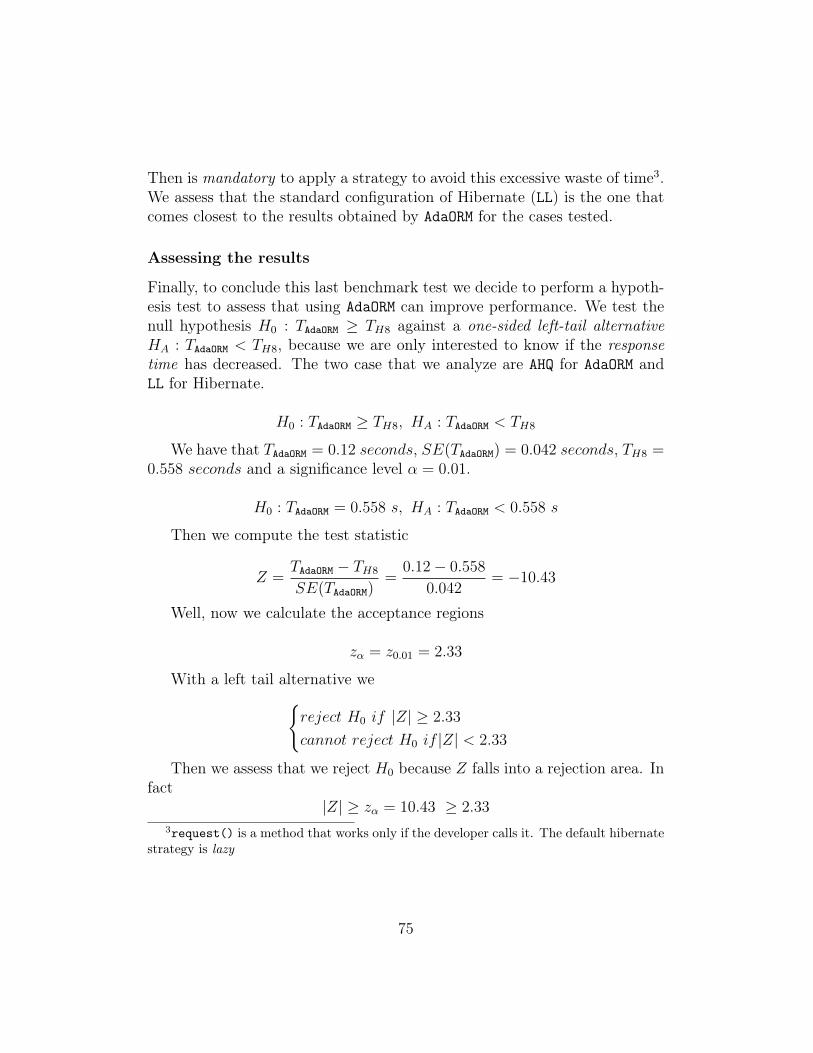
Then is mandatory to apply a strategy to avoid this excessive waste of time3.We assess that the standard configuration of Hibernate (LL) is the one thatcomes closest to the results obtained by AdaORM for the cases tested.

Assessing the results

Finally, to conclude this last benchmark test we decide to perform a hypoth-esis test to assess that using AdaORM can improve performance. We test thenull hypothesis H0 : TAdaORM ≥ TH8 against a one-sided left-tail alternativeHA : TAdaORM < TH8, because we are only interested to know if the responsetime has decreased. The two case that we analyze are AHQ for AdaORM andLL for Hibernate.

H0 : TAdaORM ≥ TH8, HA : TAdaORM < TH8

We have that TAdaORM = 0.12 seconds, SE(TAdaORM) = 0.042 seconds, TH8 =0.558 seconds and a significance level α = 0.01.

H0 : TAdaORM = 0.558 s, HA : TAdaORM < 0.558 s

Then we compute the test statistic

Z =TAdaORM − TH8

SE(TAdaORM)=

0.12− 0.558

0.042= −10.43

Well, now we calculate the acceptance regions

zα = z0.01 = 2.33

With a left tail alternative we{reject H0 if |Z| ≥ 2.33

cannot reject H0 if |Z| < 2.33

Then we assess that we reject H0 because Z falls into a rejection area. Infact

|Z| ≥ zα = 10.43 ≥ 2.33

3request() is a method that works only if the developer calls it. The default hibernatestrategy is lazy

75

Conclusion

We can assess that AdaORM works better than Hibernate in the analyzed cases.However, we must say that these results should be considered carefully. Infact, Hibernate provides many features that we have not incorporated inAdaORM and then an absolute comparison is unfair. However, the conclusionthat dynamic configuration of the fetching strategy can improve the perfor-mance drastically emerge from the experiments in a clear way. Indeed, wethink that the inclusion of an adapting strategy can be a good improvementin object relational mapping tools as Hibernate.

4.4 Queueing system analysisAccording to the definitions in Chapter 2, now we analyze the theoreticalqueueing model behind AdaORM [12]. In Figure 4.29 we can see the closednetwork designed to perform the previous tests and now defining metrics.

4.4.1 Adaptive Heavy Query

First of all, we define the analysis context. The parameters used in this anal-ysis are obtained from Adaptive Heavy Query (AHQ) service rate describedin the previous section. We assume that the service times are exponentiallydistributed with FCFS scheduling discipline. Under these assumptions, wecan compute the expected response time and the throughput. Let the ser-vice time of AHQ be Tservice = 0.12 seconds and thinking time Tthinking = 2seconds. Tservice is the total time required by a customer to be served. Split-ting this time in each station we obtain that the time spent over softwarelayer (AdaORM ) is Tsw = 0.1 seconds and time spent at the database isTdatabase = 0.02 seconds. According to those values we can start our analysis.

Variable SecondsTthinking 2.0 sTsw 0.1 s

Tdatabase 0.02 s

Table 4.12: Expected service time at each station

76

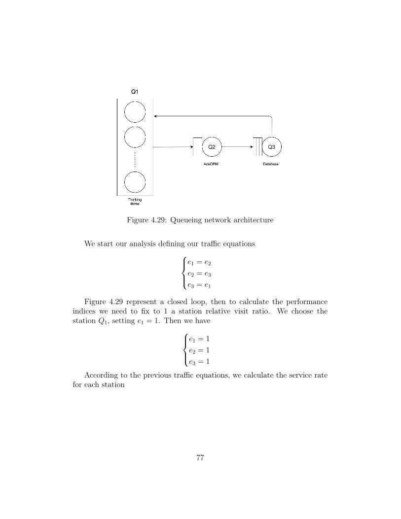
Figure 4.29: Queueing network architecture

We start our analysis defining our traffic equationse1 = e2

e2 = e3

e3 = e1

Figure 4.29 represent a closed loop, then to calculate the performanceindices we need to fix to 1 a station relative visit ratio. We choose thestation Q1, setting e1 = 1. Then we have

e1 = 1

e2 = 1

e3 = 1

According to the previous traffic equations, we calculate the service ratefor each station

77

µ1 =1

Tthinking=

1

2.0= 0.5 s−1

µ2 =1

Tsw=

1

0.1= 10 s−1

µ3 =1

Tdatabase=

1

0.02= 50 s−1

(4.1)

and solving the next equation we can retrieve the service demand for eachstation to find the slowest component.

D1 =e1

µ1

=1

0.5= 2.0 s

D2 =e2

µ2

=1

10= 0.1 s

D3 =e3

µ3

=1

50= 0.02 s

(4.2)

from previous results we have not take into account the thinking time aspossible bottleneck. Then the slowest component is the software layer, withservice time is Db = D2 = 0.1.

Now, we want to discover what could be our maximum level of multipro-gramming. Using the theoretical results deriving from operational analysison the upper bounds of the throughput we can achieve our intent. We knowthese bounds are given by

X ≤ min(1

Db

,N

D + Z)

where D is the sum of each service demand, Db the service demand of thebottleneck, N is the level of multiprogramming and Z is the thinking time.

78

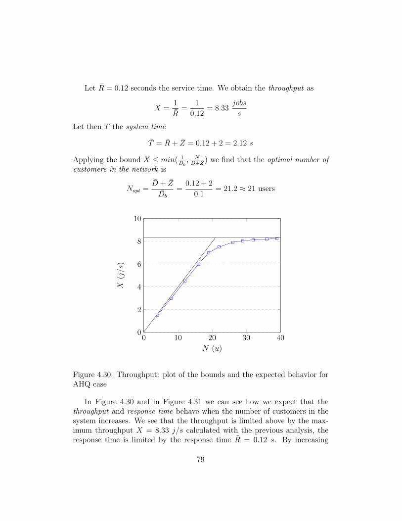
Let R̄ = 0.12 seconds the service time. We obtain the throughput as

X =1

R̄=

1

0.12= 8.33

jobs

s

Let then T the system time

T̄ = R̄ + Z̄ = 0.12 + 2 = 2.12 s

Applying the bound X ≤ min( 1Db, ND+Z

) we find that the optimal number ofcustomers in the network is

Nopt =D̄ + Z̄

D̄b

=0.12 + 2

0.1= 21.2 ≈ 21 users

0 10 20 30 400

2

4

6

8

10

N (u)

X(j/s

)

Figure 4.30: Throughput: plot of the bounds and the expected behavior forAHQ case

In Figure 4.30 and in Figure 4.31 we can see how we expect that thethroughput and response time behave when the number of customers in thesystem increases. We see that the throughput is limited above by the max-imum throughput X = 8.33 j/s calculated with the previous analysis, theresponse time is limited by the response time R̄ = 0.12 s. By increasing

79

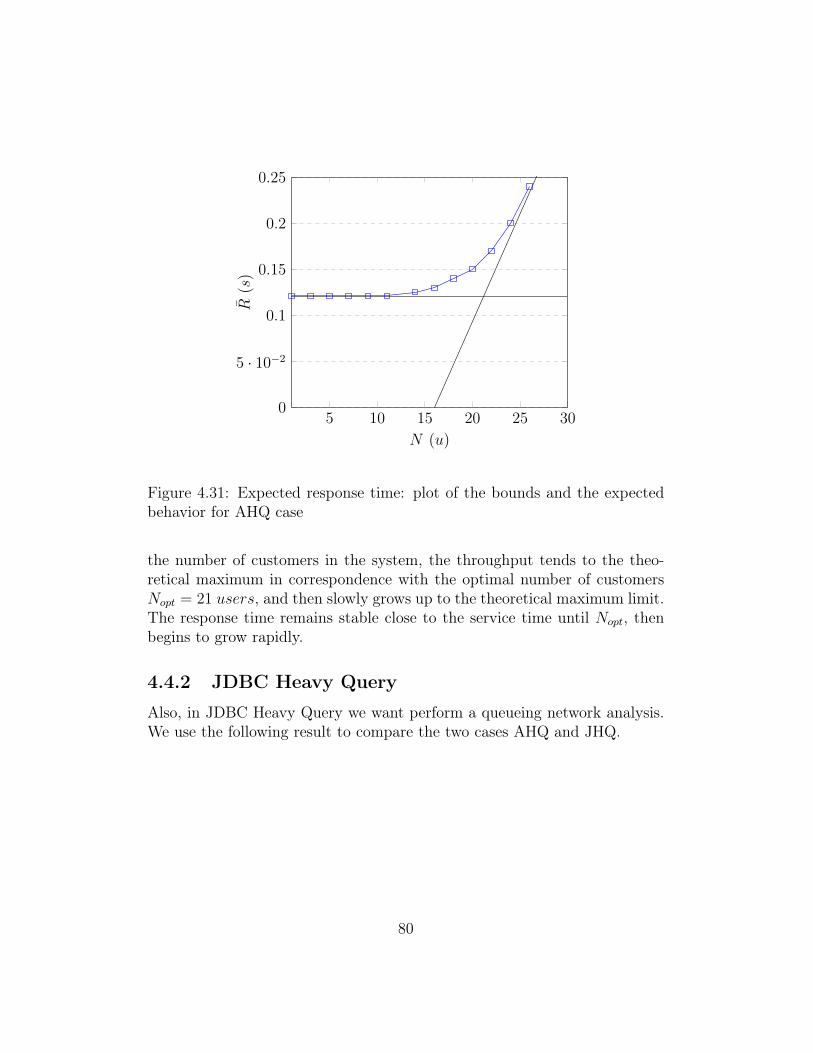
5 10 15 20 25 300

5 · 10−2

0.1

0.15

0.2

0.25

N (u)

R̄(s

)

Figure 4.31: Expected response time: plot of the bounds and the expectedbehavior for AHQ case

the number of customers in the system, the throughput tends to the theo-retical maximum in correspondence with the optimal number of customersNopt = 21 users, and then slowly grows up to the theoretical maximum limit.The response time remains stable close to the service time until Nopt, thenbegins to grow rapidly.

4.4.2 JDBC Heavy Query

Also, in JDBC Heavy Query we want perform a queueing network analysis.We use the following result to compare the two cases AHQ and JHQ.

80

Tthinking = 2 s

Tservice = 0.38 s

Tsw = 0.03 s

Tdatabase = 0.35 s

(4.3)

service times exponentially distributed with FCFS scheduling disciplinefor JHQ cases. We define our traffic equations, that define a relation amongthe relative visit ratios in closed queueing networks.

e1 = e2

e2 = e3

e3 = e1

And setting also in this case e1 = 1 we havee1 = 1

e2 = 1

e3 = 1

So, we obtain the next results

µ1 =1

Tthinking=

1

2.0= 0.5 s−1

µ2 =1

Tsw=

1

0.03= 33.3 s−1

µ3 =1

Tdatabase=

1

0.35= 2.86 s−1

(4.4)

and to get the bottleneck we must solve the follow equations, finding theslowest component

81

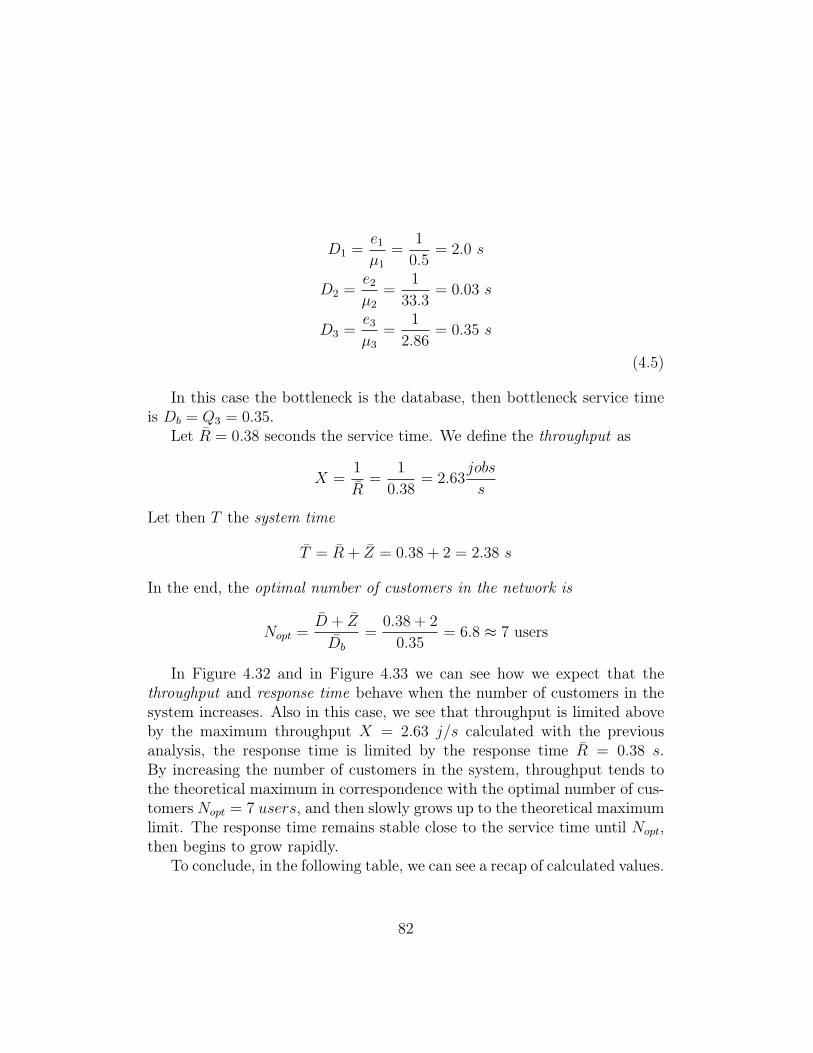
D1 =e1

µ1

=1

0.5= 2.0 s

D2 =e2

µ2

=1

33.3= 0.03 s

D3 =e3

µ3

=1

2.86= 0.35 s

(4.5)

In this case the bottleneck is the database, then bottleneck service timeis Db = Q3 = 0.35.

Let R̄ = 0.38 seconds the service time. We define the throughput as

X =1

R̄=

1

0.38= 2.63

jobs

s

Let then T the system time

T̄ = R̄ + Z̄ = 0.38 + 2 = 2.38 s

In the end, the optimal number of customers in the network is

Nopt =D̄ + Z̄

D̄b

=0.38 + 2

0.35= 6.8 ≈ 7 users

In Figure 4.32 and in Figure 4.33 we can see how we expect that thethroughput and response time behave when the number of customers in thesystem increases. Also in this case, we see that throughput is limited aboveby the maximum throughput X = 2.63 j/s calculated with the previousanalysis, the response time is limited by the response time R̄ = 0.38 s.By increasing the number of customers in the system, throughput tends tothe theoretical maximum in correspondence with the optimal number of cus-tomers Nopt = 7 users, and then slowly grows up to the theoretical maximumlimit. The response time remains stable close to the service time until Nopt,then begins to grow rapidly.

To conclude, in the following table, we can see a recap of calculated values.

82

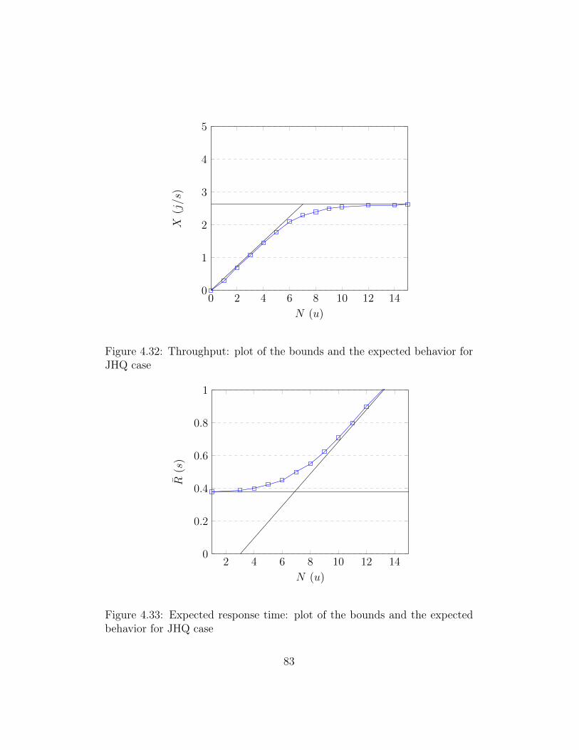
0 2 4 6 8 10 12 140

1

2

3

4

5

N (u)

X(j/s

)

Figure 4.32: Throughput: plot of the bounds and the expected behavior forJHQ case

2 4 6 8 10 12 140

0.2

0.4

0.6

0.8

1

N (u)

R̄(s

)

Figure 4.33: Expected response time: plot of the bounds and the expectedbehavior for JHQ case

83

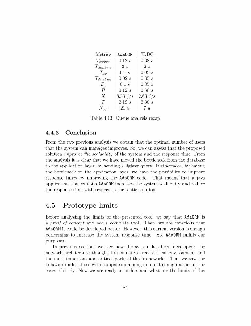
Metrics AdaORM JDBCTservice 0.12 s 0.38 sTthinking 2 s 2 sTsw 0.1 s 0.03 s

Tdatabase 0.02 s 0.35 sDb 0.1 s 0.35 sR̄ 0.12 s 0.38 sX 8.33 j/s 2.63 j/sT 2.12 s 2.38 sNopt 21 u 7 u

Table 4.13: Queue analysis recap

4.4.3 Conclusion

From the two previous analysis we obtain that the optimal number of usersthat the system can manages improves. So, we can assess that the proposedsolution improves the scalability of the system and the response time. Fromthe analysis it is clear that we have moved the bottleneck from the databaseto the application layer, by sending a lighter query. Furthermore, by havingthe bottleneck on the application layer, we have the possibility to improveresponse times by improving the AdaORM code. That means that a javaapplication that exploits AdaORM increases the system scalability and reducethe response time with respect to the static solution.

4.5 Prototype limitsBefore analyzing the limits of the presented tool, we say that AdaORM isa proof of concept and not a complete tool. Then, we are conscious thatAdaORM it could be developed better. However, this current version is enoughperforming to increase the system response time. So, AdaORM fulfills ourpurposes.

In previous sections we saw how the system has been developed: thenetwork architecture thought to simulate a real critical environment andthe most important and critical parts of the framework. Then, we saw thebehavior under stress with comparison among different configurations of thecases of study. Now we are ready to understand what are the limits of this

84

type of implementation.

4.5.1 Concurrency

AdaORM has been developed without considering big improvements given byintroduction of concurrency. The only threads introduced were used to recordstatistics asynchronously into the system database. Introducing concurrencyat beans creation or prediction computation can improve response time.

4.5.2 System database

SQLiteis not a client-server database engine. It is though to be included intoa client program, but its application in this case can be enough performaning.However, if we would implement concurrency parts, we should change DBMSbecause SQLite does not suggest to manage high degree of parallelism[18].

4.5.3 Usability

Hibernate implements mapping using annotations. Also, we can find sometools that, given the database schema generate the respective class withannotations. AdaORM is a very young ORM project born to assess if is possibletrying to guess the best result set through the collected statistics.

Given this observations is "normal" that there are some imperfection andits integration with an RDBMS and java application is slow. The mappingbetween POJO object and database tables can be improved, but this im-provement would not changes the goals of this project.

In this chapter, we have seen some cases where is convenient use AdaORMand other where AdaORM perform worse than a static solution. We haveseen how a good prediction can boost our execution time, and we have alsoseen how a wrong prediction can gives us a little or a big waste of time.However, the algorithm guarantees us that in case the program’s "habits"change by making us make a mistake, AdaORM will learn how to adapt to thecurrent behavior, offering us again high performance and avoiding long andcomplicated code maintenance.

85

86

Chapter 5

Conclusions and Future Works

In this thesis we have addressed the problem of the dynamic configuration ofORM tools. We have proposed AdaORM, a prototype tool that decides policyof data fetching at runtime, according to the user behavior. To assess theconvenience of the tool we have performed many experiments, performancetests and we have compared the results with state of art solutions.

It is evident that, using AdaORM , the response time and the system per-formance improve when the predictor guesses the right query to submit. Thegreat improvement is given in that by guessing the right result set, the sys-tem will not need to make new connections to the database, or to retrieveunnecessary data, reducing response times. Instead, when AdaORM misses thequery to execute, especially in the case in which it loads a smaller dataset, itwill have large delays, than the static solution, due to the multiple databaseconnections necessary to collect usage statistics. If it loads a larger dataset,we will still have delays comparable to the static solution since the servicetimes are dominant by the application needs.

However, we know that is always do better. This development is onlya proof of concept to assess that is possible improve execution time andsystem load handling the statement before its execution and exploiting joinelimination optimization.

Developing the project we realized that it is possible to introduce inter-esting and convenient optimizations to improve the impact of the ORM inthe system and improve the data prediction.

In conclusion, the dynamic decision of the policy of fetching is very usefulin those cases in which the programmer cannot know which will be the usagepattern of the application and hence the static decision may lead too poor

87

performance. The overhead introduced by predictor is tolerable where theapplication is data intensive while it may become heavy otherwise.

5.1 Data predictionProposed work 1: Collecting many information about execution and datautilization, we can apply different data mining algorithm. For example, wecan find a pattern over the data using PaNDa+ algorithm [13]. The patternwill be the set of columns called together most frequently. Balancing thethresholds using the system load, we can shrink our prediction: with highersystem load we will allow less noyse, with lower system load we will allowmore noyse, then more columns.

Proposed work 2: An other possible prediction implementation could bethe use of a machine learning algorithm. We can use an algorithm that canlearn when we need a particular set of columns.

Proposed work 3: Another interesting feature that could be implementedis the introduction of the clustering of statistics to make the predictor moreflexible to change. In fact, calculating the predictions on many values, if thebehavior of the system changes, the change in the predictions will not be asfast.

Proposed work 4: In the end, the last possible future work that we wantto suggest changing the core of the prediction from columns to the tables. Infact, after the prediction of a column, we require the fetching of all requestedcolumns that belongs to the same table because it is more convenient loadnow the information. Changing the observed elements, the granularity of thesystem changes but the predicted result set does not change. In this way, wecan store less data and the predictor will do less computation.

5.2 Cost impactProposed work 1: By introducing asynchronous calls and promises, wecan improve system performance. In fact, while AdaORM retrieves information

88

from the database, it is possible to use another thread (or an asynchronouscall) to start composing an object.

Proposed work 2: In the current version, the prediction will be performedafter its request, caching the results for 10 requests before re computation.However, computing the prediction after its request can decrease the speedof the system. To avoid this issue, it is possible an offline prediction. Anoffline prediction is a prediction performed not after its requests, but afterthe fetching of the result set using the cached predicted query. Also, we canplan the new query computation by keeping in mind the system load: whenthe system is unloading we can perform the planned execution after a lessnumber of requests.

Proposed work 3: Applying the Data prediction proposed work 3 we canreduce the cost to perform prediction. In fact, |tables| ≤ |columns|, then, theasymptotically cost of the prediction function change in terms of cardinalityfrom columns to tables.

89

90

Chapter 6

Acknowledgements

This has been a long and demanding course of study, but I have come toits end. Every single step towards the achievement of this title has costme effort and sweat. I must thank my determination, my commitment, myorganization and my resilience for having supported me every single day ofthe past few years to get where I am here today.

I want to thank my supervisor Andrea Marin, who has patiently followedme remotely, with all the difficulties of the case, in my latest interesting andstimulating academic project. Also, I want to thank him since he acceptedme to work with him. I also want to thank professor Alvise Spanò, whosedeep knowledge in software architecture, has given me some excellent adviceon how to model AdaORM . Thanks also to Stefano Calzavara, who madehimself available in giving me tips about DBMS problems. Thanks to myboss, who gave me a lot of flexibility to follow my studies. Thanks to myfamily, who gave me the opportunity to attend this academic path and andthey bear me even in my worst moments.

Last but not least, all my friends, who have always been there, whosupported me in difficult times and with whom we celebrated in moments ofjoy. I want to thank all my fellow students with whom I spent entire days,first shoulder to shoulder, then by teleconference, to complete projects andto prepare exams. Teamwork has made us stronger.

This is not only the end of a course of study for me, but this is the finishof an era. From tomorrow my life will never be the same, again. But, I can’twait to face all the new challenges that life has to offer me.

Thank you again, Paolo.

91

List of Figures

1.1 Hibernate architecture . . . . . . . . . . . . . . . . . . . . . . 9

2.1 UML representation of Strategy pattern . . . . . . . . . . . . 182.2 UML representation of Decorator pattern . . . . . . . . . . . . 192.3 UML representation of DAO pattern . . . . . . . . . . . . . . 202.4 Acceptance and rejection regions . . . . . . . . . . . . . . . . 28

3.1 AdaORM architecture . . . . . . . . . . . . . . . . . . . . . . . . 35

4.1 Two tier architecture implemented . . . . . . . . . . . . . . . . 424.2 Data set employees schema . . . . . . . . . . . . . . . . . . . . 464.3 MySQL execution time between different queries . . . . . . . . 494.4 PostgreSQL execution time between different queries . . . . . 514.5 DB2 execution time between different queries . . . . . . . . . 534.6 Book database UML schema . . . . . . . . . . . . . . . . . . . 564.7 Home made benchmark comparison - guessed . . . . . . . . . 584.8 Execution time of queries in Heavy mode from custom bench-

mark . . . . . . . . . . . . . . . . . . . . . . . . . . . . . . . . 594.9 Execution time of queries in Light mode from custom benchmark 594.10 Home made benchmark comparison - not guessed . . . . . . . 604.11 Tsung benchmark service rate comparison . . . . . . . . . . . 634.12 System response time in AHQ . . . . . . . . . . . . . . . . . . 634.13 System response time in JHQ . . . . . . . . . . . . . . . . . . 644.14 System response time in ALQ . . . . . . . . . . . . . . . . . . 644.15 System response time in JLQ . . . . . . . . . . . . . . . . . . 654.16 AHQ CPU load . . . . . . . . . . . . . . . . . . . . . . . . . . 654.17 JHQ CPU load . . . . . . . . . . . . . . . . . . . . . . . . . . 664.18 ALQ CPU load . . . . . . . . . . . . . . . . . . . . . . . . . . 674.19 JLQ CPU load . . . . . . . . . . . . . . . . . . . . . . . . . . 67

92

4.20 AHQ memory free . . . . . . . . . . . . . . . . . . . . . . . . 684.21 JHQ memory free . . . . . . . . . . . . . . . . . . . . . . . . . 684.22 ALQ memory free . . . . . . . . . . . . . . . . . . . . . . . . . 694.23 JLQ memory free . . . . . . . . . . . . . . . . . . . . . . . . . 694.24 AHQ concurrent users . . . . . . . . . . . . . . . . . . . . . . 704.25 JHQ concurrent users . . . . . . . . . . . . . . . . . . . . . . . 704.26 ALQ concurrent users . . . . . . . . . . . . . . . . . . . . . . 714.27 JLQ concurrent users . . . . . . . . . . . . . . . . . . . . . . . 714.28 Hibernate and AdaORM benchmark comparison . . . . . . . . . 744.29 Queueing network architecture . . . . . . . . . . . . . . . . . . 774.30 Throughput: plot of the bounds and the expected behavior

for AHQ case . . . . . . . . . . . . . . . . . . . . . . . . . . . 794.31 Expected response time: plot of the bounds and the expected

behavior for AHQ case . . . . . . . . . . . . . . . . . . . . . . 804.32 Throughput: plot of the bounds and the expected behavior

for JHQ case . . . . . . . . . . . . . . . . . . . . . . . . . . . 834.33 Expected response time: plot of the bounds and the expected

behavior for JHQ case . . . . . . . . . . . . . . . . . . . . . . 83

93

List of Tables

1.1 Matching principal ORMs . . . . . . . . . . . . . . . . . . . . 11

2.1 Comparison between SQL vs NoSQL . . . . . . . . . . . . . . 172.2 Recap of different type of alternative hypothesis . . . . . . . . 28

4.1 Developing machine skills . . . . . . . . . . . . . . . . . . . . 434.2 Test machine skills . . . . . . . . . . . . . . . . . . . . . . . . 434.3 MySQL benchmark with mysqlslap results . . . . . . . . . . . 484.4 Postgres benchmark results . . . . . . . . . . . . . . . . . . . 504.5 DB2 benchmark results . . . . . . . . . . . . . . . . . . . . . . 524.6 Tables with their cardinality in Books database for IBM DB2 554.7 Execution time when AdaORM guesses the query to execute . . 574.8 Execution time when AdaORM does not guess the query to execute 604.9 Service time recap in seconds . . . . . . . . . . . . . . . . . . 624.10 Expected response time recap . . . . . . . . . . . . . . . . . . 724.11 Hibernate and AdaORM expected response time . . . . . . . . . 744.12 Expected service time at each station . . . . . . . . . . . . . . 764.13 Queue analysis recap . . . . . . . . . . . . . . . . . . . . . . . 84

94

Bibliography

[1] Antonio Albano, Dario Colazzo, Giorgio Ghelli, and Renzo Orsini. Re-lational dbms internals, 2015.

[2] Sinan Si Alhir. Learning Uml. " O’Reilly Media, Inc.", 2003.

[3] Michael Baron. Probability and statistics for computer scientists. CRCPress, 2014.

[4] Db2Tutorial. Db2tutorial - book database. https://cdn.db2tutorial.com/wp-content/uploads/2019/06/books.zip.

[5] Docker. Docker. https://www.docker.com/.

[6] J. Dollimore G. Coulouris and T. Kindberg. Distributed Systems: con-cepts and design. Addison Wesley Professional, 5 edition, 2011.

[7] Erich Gamma. Design patterns: elements of reusable object-orientedsoftware. Pearson Education India, 1995.

[8] IBM. db2batch - benchmark tool command. https://www.ibm.com/support/producthub/db2/docs/content/SSEPGG_11.5.0/com.ibm.db2.luw.admin.cmd.doc/doc/r0002043.html.

[9] IBM. db2expln - sql and xquery explain command. https://www.ibm.com/support/knowledgecenter/SSEPGG_11.1.0/com.ibm.db2.luw.admin.cmd.doc/doc/r0005736.html.

[10] IBM. Ibm db2 – data management software. https://www.ibm.com/analytics/db2.

[11] Javapoint. Mysql features. https://www.javatpoint.com/mysql-features.

95

[12] Edward D Lazowska, John Zahorjan, G Scott Graham, and Kenneth CSevcik. Quantitative system performance: computer system analysis us-ing queueing network models. Prentice-Hall, Inc., 1984.

[13] Claudio Lucchese, Salvatore Orlando, and Raffaele Perego. A unifyingframework for mining approximate top-k binary patterns. IEEE Trans-actions on Knowledge and Data Engineering, 26(12):2900–2913, 2013.

[14] Lukaseder. Join elimination: An essential optimiser feature for advancedsql usage, September 2017. https://blog.jooq.org/2017/09/01/join-elimination-an-essential-optimiser-feature-for-advanced-sql-usage/.

[15] N. Niclausse. Tsung, 06 2017. http://tsung.erlang-projects.org/.

[16] Oracle. Mysql slap. https://dev.mysql.com/doc/refman/8.0/en/mysqlslap.html.

[17] Oracle. Sakila structure. https://dev.mysql.com/doc/employee/en/sakila-structure.html.

[18] Mike Owens. The definitive guide to SQLite. Apress, 2006.

[19] Spring. Spring-boot, June 2020. https://spring.io/projects/spring-boot.

[20] Wumpz. Jsqlparser. https://github.com/JSQLParser/JSqlParser.

96