adaptive sequential experiments with unknown information flows · adaptive sequential experiments...

Adaptive Sequential Experiments with Unknown Information Flows

Yonatan Gur

Stanford University

Ahmadreza Momeni∗

Stanford University

February 7, 2019

Abstract

An agent facing sequential decisions that are characterized by partial feedback needs to strike a

balance between maximizing immediate payoffs based on available information, and acquiring new

information that may be essential for maximizing future payoffs. This trade-off is captured by the

multi-armed bandit (MAB) framework that has been studied and applied under strong assumptions

on the information collection process: at each time epoch a single observation is collected on the

action that was selected at that epoch. However, in many practical settings additional information

may become available between pulls, and might be essential for achieving good performance. We

introduce a generalized MAB formulation that relaxes the strong assumptions on the information

collection process, and in which auxiliary information on each arm may appear arbitrarily over time.

By obtaining matching lower and upper bounds, we characterize the (regret) complexity of this family

of MAB problems as a function of the information flows, and study how salient characteristics of

the information impact policy design and achievable performance. We introduce a broad adaptive

exploration approach for designing policies that, without any prior knowledge on the information

arrival process, attain the best performance (regret rate) that is achievable when the information

arrival process is a priori known. Our approach is based on adjusting MAB policies designed to

perform well in the absence of auxiliary information by using dynamically customized virtual time

indexes to endogenously control the exploration rate of the policy. We demonstrate the effectiveness

of our approach through establishing performance bounds and evaluating numerically the performance

of adjusted well-known MAB policies. Our study demonstrates how decision-making policies designed

to perform well with very little information can be adjusted to also guarantee optimality in more

information-abundant settings.

Keywords: sequential decisions, data-driven decisions, online learning, adaptive algorithms, multi-

armed bandits, exploration-exploitation, minimax regret.

1 Introduction

1.1 Background and motivation

In the presence of uncertainty and partial feedback on payoffs, an agent that faces a sequence of decisions

needs to strike a balance between maximizing instantaneous performance indicators (such as revenue)

and collecting valuable information that is essential for optimizing future decisions. A well-studied

∗The authors are grateful to Omar Besbes and Lawrence M. Wein for their valuable comments. Correspondence:[email protected], [email protected].

1

framework that captures this trade-off between new information acquisition (exploration), and optimizing

payoffs based on available information (exploitation) is the one of multi-armed bandits (MAB) that first

emerged in Thompson (1933) in the context of drug testing, and was later extended by Robbins (1952)

to a more general setting. In this framework, an agent needs to repeatedly choose between K arms,

where at each trial the agent pulls one of the arms, and receives a reward. In the formulation of this

problem (known as the stochastic MAB setting), rewards from each arm are assumed to be identically

distributed and independent across trails and arms. The objective of the agent is to maximize the

cumulative return over a certain time horizon, and the performance criterion is the so-called regret : the

expected difference between the cumulative reward received by the agent and the reward accumulated by

a hypothetical benchmark, referred to as oracle, who holds prior information and the reward distribution

of each arm (and thus repeatedly selects the arm with the highest expected reward). Since its inception,

this framework has been analyzed under different assumptions to study a variety of applications including

clinical trials (Zelen 1969), strategic pricing (Bergemann and Valimaki 1996), packet routing (Awerbuch

and Kleinberg 2004), online auctions (Kleinberg and Leighton 2003), online advertising (Pandey et al.

2007), and product recommendations (Madani and DeCoste 2005, Li et al. 2010), among many others.

Classical MAB settings (including the ones used in the above applications) focus on balancing

exploration and exploitation in environments where at each period a reward observation is collected

only on the arm that is selected by the policy at that time period. However, in many practical settings

additional information (that may take various forms, see example below) may become available between

decision epochs and may be relevant also to arms that were not selected recently. While in many

real-world scenarios utilizing such information flows may be fundamental for achieving good performance,

the MAB framework does not account for the extent to which such information flows may impact the

design of learning policies and the performance such policies may achieve. We next discuss one concrete

application domain to which MAB policies have been commonly applied in the past, and in which such

auxiliary information is a fundamental part of the problem.

The case of cold-start problems in online product recommendations. Product recommendation

systems are widely deployed in the web nowadays, with the objective of helping users navigate through

content and consumer products while increasing volume and revenue for service and e-commerce platforms.

These systems commonly apply various collaborative filtering and content-based filtering techniques

that leverage information such as explicit and implicit preferences of users, product consumption and

popularity, and consumer ratings (see, e.g., Hill et al. 1995, Konstan et al. 1997, Breese et al. 1998).

While effective when ample information is available on products and consumers, these techniques tend

to perform poorly encountering consumers or products that are new to the system and have little

or no trace of activity. This phenomenon, termed as the cold-start problem, has been documented

2

and studied extensively in the literature; see, e.g., Schein et al. (2002), Park and Chu (2009), and

references therein. With this problem in mind, several MAB formulations were suggested and applied for

designing recommendation algorithms that effectively balance information acquisition and instantaneous

revenue maximization, where arms represent candidate recommendations; see the overview in Madani

and DeCoste (2005), as well as later studies by Agarwal et al. (2009), Caron and Bhagat (2013), Tang

et al. (2014), and Wang et al. (2017). Aligned with traditional MAB frameworks, these studies consider

settings where in each time period observations are obtained only for items that are recommended by the

system at that period. However, additional browsing and consumption information may be maintained

in parallel to the sequential recommendation process, as a significant fraction of website traffic may

take place through means other than recommendation systems (for example, consumers that arrive to

product pages directly from external search engines); see browsing data analysis in Sharma and Yan

(2013) and Mulpuru (2006), as well as Grau (2009), who estimate that recommendation systems are

responsible to only 10-30% of site traffic and revenue. This additional information could potentially be

used to better estimate the “reward” from recommending new products and improve the performance of

recommendation algorithms facing a cold-start problem (we will discuss in more detail how this could be

done after laying out our formulation).

Key challenges and research questions. The availability of additional information (relative to the

information collection process that is assumed in classical MAB formulations) fundamentally impacts

the design of learning policies and the way a decision maker should balance exploration and exploitation.

When additional information is available one may potentially obtain better estimators for the mean

rewards, and therefore may need to “sacrifice” less decision epochs for exploration. While this intuition

suggests that exploration can be reduced in the presence of additional information, it is a priori not

clear how exactly should the appropriate exploration rate depend on the information flows. Moreover,

monitoring the exploration levels in real time in the presence of arbitrary information flows introduces

additional challenges that have distinct practical relevance. Most importantly, an optimal exploration

rate may depend on several characteristics of the information arrival process, such as the amount of

information that arrives on each arm, as well as the time at which this information appears (e.g., early

on versus later on along the decision horizon). Since it may be hard to predict upfront the salient

characteristics of arbitrary information flows, an important challenge is to adapt in real time to an

a priori unknown information arrival process and adjust the exploration rate accordingly in order to

achieve the performance that is optimal (or near optimal) under prior knowledge of the sample path of

information arrivals. This paper is concerned with addressing these challenges.

The main research questions we study in this paper are: (i) How does the best achievable performance

(in terms of minimax complexity) that characterizes a sequential decision problem change in the presence

3

of arbitrary information flows? (ii) How should the design of efficient decision-making policies change in

the presence of such information flows? (iii) How are achievable performance and policy design affected

by the characteristics of the information arrival process, such as the frequency of observations, and their

timing? (iv) How can a decision maker adapt to a priori unknown and arbitrary information arrival

processes in a manner that guarantees the (near) optimal performance that is achievable under ex-ante

knowledge of these processes (“the best of all worlds”)?

1.2 Main contributions

The main contribution of this paper lies in introducing a new, generalized MAB framework with unknown

and arbitrary information flows, characterizing the regret complexity of this broad class of MAB problems,

and proposing a general policy design approach that demonstrates how effective decision-making policies

designed to perform well with very little information can be adjusted in a practical manner that

guarantees optimality in information-abundant settings characterized by arbitrary and a priori unknown

information flows. More specifically, our contribution is along the following dimensions.

(1) Modeling. We formulate a new class of MAB problems in the presence of a priori unknown

information flows that generalizes the classical stochastic MAB framework, by relaxing strong assumptions

that are typically imposed on the information collection process. Our formulation considers a priori

unknown information flows that correspond to the different arms and allows information to arrive at

arbitrary rate and time. Our formulation therefore captures a large variety of real-world phenomena, yet

maintains mathematical tractability.

(2) Analysis. We establish lower bounds on the performance that is achievable by any non-anticipating

policy in the presence of unknown information flows, where performance is measured in terms of regret

relative to the performance of an oracle that constantly selects the arm with the highest mean reward.

We further show that our lower bounds can be achieved through suitable policy design. These results

identify the minimax complexity associated with the MAB problem with unknown information flows,

as a function of the information arrivals process, as well as other problem characteristics such as the

length of the problem horizon, the number of arms, and parametric characteristics of the family of

reward distributions. In particular, we obtain a spectrum of minimax regret rates ranging from the

classical regret rates that appear in the stochastic MAB literature when there is no or very little auxiliary

information, to a constant regret (independent of the length of the decision horizon) when information

arrives frequently and/or early enough.

(3) Policy design. We introduce a general adaptive exploration approach for designing policies that,

without any prior knowledge on the auxiliary information flows, approximate the best performance that

is achievable when the information arrival process is known in advance. This “best of all worlds” type of

4

guarantee implies that rate optimality is achieved uniformly over the general class of information flows

at hand (including the case with no information flows, where classical guarantees are recovered).

Our approach relies on using endogenous exploration rates that depend on the amount of information

that becomes available over time. In particular, it is based on adjusting in real time the effective

exploration rate of MAB policies that were designed to perform well in the absence of any auxiliary

information flows, while leveraging the structure of said policies. More precisely, various well-known

MAB policies govern the rate at which sub-optimal options are explored through some monotonously

decreasing function of the time period, where the precise structure of said function may change from

one algorithm to another. Our approach leverages the optimality of these functional structures in the

absence of any auxiliary information flows, while replacing the time index with virtual time indexes

that are dynamically updated based on information arrivals. Whenever auxiliary information on a

certain arm arrives, the virtual time index that is associated with that arm is advanced using a carefully

selected multiplicative factor, and thus the rate at which the policy is experimenting with that arm is

reduced. We demonstrate the effectiveness and practicality of the adaptive exploration approach through

establishing performance bounds and evaluating numerically the performance of the adjusted versions of

well-known MAB policies.

(4) Reactive information flows. Our formulation focuses on information flows that are arbitrary and

unknown to the decision maker, but are fixed upfront and independent of the decision path of the policy.

In §6 of the paper we extend our framework to consider a broad class of information flows that are

reactive to the past actions of the decision-making policy. We study the impact endogenous information

flows may have on the achievable performance, and establish the optimality of the adaptive exploration

approach for a broad class of endogenous information flows.

1.3 Related work

Multi-armed bandits. For a comprehensive overview of MAB formulations we refer the readers to the

monographs by Berry and Fristedt (1985) and Gittins et al. (2011) for Bayesian / dynamic programming

formulations, as well as to Cesa-Bianchi and Lugosi (2006) and Bubeck et al. (2012) that cover the

machine learning literature and the so-called adversarial setting. A sharp regret characterization for the

more traditional framework (random rewards realized from stationary distributions), often referred to as

the stochastic MAB problem, was first established by Lai and Robbins (1985), followed by analysis of

important policies designed for the stochastic framework, such as the ε-greedy, UCB1, and Thompson

sampling; see, e.g., Auer, Cesa-Bianchi, and Fischer (2002), as well as Agrawal and Goyal (2013).

The MAB framework focuses on balancing exploration and exploitation, typically under very little

assumptions on the distribution of rewards, but with very specific assumptions on the future information

5

collection process. In particular, optimal policy design is typically predicated on the assumption that

at each period a reward observation is collected only on the arm that is selected by the policy at that

time period (exceptions to this common information structure are discussed below). In that sense,

such policy design does not account for information (e.g., that may arrive between pulls) that may

be available in many practical settings, and that might be essential for achieving good performance.

In the current paper we relax the information structure of the classical MAB framework by allowing

arbitrary information arrival processes. Our focus is on: (i) studying the impact of the information

arrival characteristics (such as frequency and timing) on policy design and achievable performance; and

(ii) adapting to a priori unknown sample path of information arrivals in real time.

As alluded to above, there are few MAB settings (and other sequential decision frameworks) in which

more information can be collected in each time period. One example is the so-called contextual MAB

setting, also referred to as bandit problem with side observations (Wang et al. 2005), or associative

bandit problem (Strehl et al. 2006), where at each trial the decision maker observes a context carrying

information about other arms. Another important example is the full-information adversarial MAB

setting, where rewards are not characterized by a stationary stochastic process but are rather arbitrary

and can even be selected by an adversary (Auer et al. 1995, Freund and Schapire 1997). In the

full-information adversarial MAB setting, at each time period the agent not only observes the reward

generated by the arm that was selected, but also observes the rewards generated by rest of the arms.

While the adversarial nature of the latter setting makes it fundamentally different in terms of achievable

performance, analysis, and policy design, from the stochastic formulation that is adopted in this paper,

it is also notable that the above settings consider very specific information structures that are a priori

known to the agent, as opposed to our formulation where the characteristics of the information flows are

arbitrary and a priori unknown.

Balancing and regulating exploration. Several papers have considered different settings of sequential

optimization with partial information and distinguished between cases where exploration is unnecessary

(a myopic decision-making policy achieves optimal performance), and cases where exploration is essential

for achieving good performance (myopic policies may lead to incomplete learning and large losses); see,

e.g., Harrison et al. (2012) and den Boer and Zwart (2013) that study policies for dynamic pricing

without knowing the demand function, Besbes and Muharremoglu (2013) for inventory management

without knowing the demand distribution, and Lee et al. (2003) in the context of technology development.

In a recent paper, Bastani et al. (2017) consider the contextual MAB framework and show that if the

distribution of the contextual information guarantees sufficient diversity, then exploration becomes

unnecessary and greedy policies can benefit from the natural exploration that is embedded in the

information diversity to achieve asymptotic optimality. In related studies, Woodroofe (1979) and Sarkar

6

(1991) consider a Bayesian one armed contextual MAB problem and show that a myopic policy achieves

is asymptotic optimal when the discount factor converges to one.

On the other hand, few papers have studied cases where exploration is not only essential but should

be particularly frequent in order to maintain optimality. For example, Besbes et al. (2014) consider a

general MAB framework where the reward distribution may change over time according to a budget of

variation, and characterize the manner in which optimal exploration rates increase as a function of said

budget. In addition, Shah et al. (2018) consider a platform in which the preferences of arriving users

may depend on the experience of previous users. They show that in such setting classical MAB policies

may under-explore, and introduce a balanced-exploration approach that results in optimal performance.

The above studies demonstrate a variety of practical settings where the extent of exploration that is

required to maintain optimality strongly depends on particular problem characteristics that may often

be a priori unknown to the decision maker. This introduces the challenge of endogenizing exploration:

dynamically adapting the rate at which a decision-making policy explores to identify the appropriate

rate of exploration and to approximate the best performance that is achievable under ex ante knowledge

of the underlying problem characteristics. In this paper we address this challenge from information

collection perspective. We identify conditions on the information arrival process that guarantee the

optimality of myopic policies, and further identify adaptive MAB policies that guarantee (near) optimal

performance without prior knowledge on the information arrival process (“best of all worlds”).

In addition, few papers considered approaches of regulating exploration rates based on a priori known

characteristics of payoff structure, in settings that are different than ours. For example, Traca and

Rudin (2015) consider an approach of regulating exploration in a setting where rewards are scaled by

an exogenous multiplier that temporally evolves in an a priori known manner, and show that in such

setting the performance of known MAB policies can be improved if exploration is increased in periods of

low reward. Another approach of regulating the exploration is studied by Komiyama et al. (2013) in a

setting that includes lock-up periods in which the agent cannot change her actions.

Adaptive algorithms. One of the challenges we address in this paper lies in designing policies that

adapt in real time to the arrival process of information, in the sense of achieving ex-post performance

which is as good (or nearly as good) as the one achievable under ex-ante knowledge on the information

arrival process. This challenge dates back to studies in the statistics literature (see Tsybakov (2008) and

references therein), and has seen recent interest in the machine learning and sequential decision making

literature streams; examples include Seldin and Slivkins (2014) that present an algorithm that achieves

(near) optimal performance in both stochastic and adversarial multi-armed bandit regimes without prior

knowledge on the nature of environment, Sani et al. (2014) that consider an online convex optimization

setting and derive algorithms that are rate optimal regardless of whether the target function is weakly

7

or strongly convex, Jadbabaie et al. (2015) that study the design of adaptive algorithms that compete

against dynamic benchmarks, and Luo and Schapire (2015) that address the problem of learning under

experts’ advices and compete in an adversarial setting against any convex combination of experts.

2 Problem formulation

In this section we formulate a class of multi-armed bandit problems with auxiliary information flows.

We note that many of our modeling assumptions can be generalized and are made only to simplify

exposition and analysis. Some generalizations of our formulation are discussed in §2.1.

Let K = {1, . . . ,K} be a set of arms (actions) and let T = {1, . . . , T} denote a sequence of decision

epochs. At each time period t ∈ T , a decision maker selects one of the K arms. When selecting an arm

k ∈ K at time t ∈ T , a reward Xk,t ∈ R is realized and observed. For each t ∈ T and k ∈ K, the reward

Xk,t is assumed to be independently drawn from some σ2-sub-Gaussian distribution with mean µk.1 We

denote the profile of rewards at time t by Xt = (X1,t, . . . , XK,t)> and the profile of mean-rewards by

µ = (µ1, . . . , µK)>. We further denote by ν = (ν1, . . . , νK)> the distribution of the rewards profile Xt.

We assume that rewards are independent across time periods and arms. We denote the highest expected

reward and the best arm by µ∗ and k∗ respectively, that is:2

µ∗ = maxk∈K{µk}, k∗ = arg max

k∈Kµk.

We denote by ∆k = µ∗−µk the difference between the expected reward of the best arm and the expected

reward of arm k. We assume prior knowledge of a positive lower bound 0 < ∆ ≤ mink∈K\{k∗}

∆k as well

as a positive number σ > 0 for which all the reward distributions are σ2-sub-Gaussian. We denote by

S = S(∆, σ2) the class of ∆-separated σ2-sub-Gaussian distribution profiles:

S(∆, σ2) :={ν = (ν1, . . . , νK)> | ∆ · 1{k 6= k∗} ≤ ∆k and E

[eλ(Xk,1−µk)

]≤ eσ2λ2/2 ∀k ∈ K,∀λ ∈ R

}.

Auxiliary information flows. Before each round t, the agent may or may not observe reward

realizations for some of the arms without pulling them. Let ηk,t ∈ {0, 1} denote the indicator of

observing an auxiliary information on arm k just before time t. We denote by ηt = (η1,t, . . . , ηK,t)>

1A real-valued random variable X is said to be sub-Gaussian if there is some σ > 0 such that for every λ ∈ R one has

Eeλ(X−EX) ≤ eσ2λ2/2.

This broad class of distributions include, for instance, Gaussian random variables, as well as any random variable with a

bounded support (if X ∈ [a, b] then X is (a−b)24

-sub-Gaussian) such as Bernoulli random variables. Notably, if a randomvariable is σ2-sub-Gaussian, it is also σ2-sub-Gaussian for all σ > σ.

2For the sake of simplicity, in the formulation and hereafter in the rest of the paper when using the arg min and arg maxoperators we assume that ties are broken in favor of the smaller index.

8

the vector of indicators ηk,t’s associated with time step t, and by H = (η1, . . . ,ηT ) the information

arrival matrix with columns ηt’s; we assume that this matrix is independent of the policy’s actions (this

assumption will be relaxed later on). If ηk,t = 1, then a random variable Yk,t ∼ νk is observed. We

denote Yt = (Y1,t, . . . , YK,t)>, and assume that the random variables Yk,t are independent across time

periods and arms and are also independent from the reward realizations Xk,t. We denote the vector of

new information received just before time t by Zt = (Z1,t, . . . , ZK,t)> where for any k one has:

Zk,t = ηk,t · Yk,t.

Admissible policies, performance, and regret. Let U be a random variable defined over a prob-

ability space (U,U ,Pu). Let πt : Rt−1 × RK×t × {0, 1}K×t × U → K for t = 1, 2, 3, . . . be measurable

functions (with some abuse of notation we also denote the action at time t by πt ∈ K) given by

πt =

π1(Z1,η1, U) t = 1,

πt(Xπt−1,t−1, . . . , Xπ1,1,Zt, . . . ,Z1,ηt, . . . ,η1, U) t = 2, 3, . . ..

The mappings {πt : t = 1, . . . , T}, together with the distribution Pu define the class of admissible policies.

We denote this class by P . We further denote by {Ht, t = 1, . . . , T} the filtration associated with a policy

π ∈ P , such that H1 = σ(Z1,η1, U), and Ht = σ({Xπs,s}t−1

s=1, {Zs}ts=1, {ηs}ts=1, U)

for all t ∈ {2, 3, . . . }.

Note that policies in P depend only on the past history of actions and observations as well as auxiliary

information arrivals, and allow for randomization via their dependence on U .

We evaluate the performance of a policy π ∈ P by the regret it incurs under information arrival

process H relative to the performance of an oracle that selects the arm with the highest expected reward.

We define the worst-case regret as follows:

RπS(H, T ) = supν∈S

Eπν

[T∑t=1

(µ∗ − µπt)

],

where the expectation Eπν [·] is taken with respect to the noisy rewards, as well as to the policy’s actions

(throughout the paper we will denote by Pπν , Eπν , and Rπν the probability, expectation, and regret when

the arms are selected according to policy π and rewards are distributed according to ν.). In addition, we

denote by R∗S(H, T ) = infπ∈PRπS(H, T ) the best achievable guaranteed performance: the minimal regret

that can be guaranteed by an admissible policy π ∈ P . In the following sections we study the magnitude

of R∗S(H, T ) as a function of the information arrival process H.

9

2.1 Discussion of model assumptions and extensions

2.1.1 Generalized information structure and the cold-start problem

In our formulation we focus on auxiliary observations that have the same distribution as reward

observations, but all our results hold for a broad family of information structures as long as unbiased

estimators of mean rewards can be constructed from the auxiliary observations, that is, when there exists

a mapping φ(·) such that E [φ(Yk,t)] = µk for each k. Notably, the compatibility with such generalized

information structure allows a variety of concrete practical applications of our analysis, including the

cold-start problem referred to in §1.1.

In particular, in the context of a product recommendation system, the reward of recommending an

item k is typically proportional to both the click-through rate (CTR) of item k, measuring the tendency

of users to click on the recommendations, as well as the conversion rate (CVR) of that item, measuring

the payoff from the actions taken by the user after the click (for example, average revenue spent once a

user arrives to the product page); namely, it is common to assume that µk = EXk,t = ck ·CTRk ·CVRk,

for some constant ck. Notably, several methods have been developed to estimate click-through rates in

the absence of historical information on new products. These include MAB-based methods that were

discussed in §1.1, as well as other methods such as ones that focus on feature-based or sematic-based

decomposition of products; see, e.g., Richardson et al. (2007) who focus on feature-based analysis, as

well as Regelson and Fain (2006) and Dave and Varma (2010) that estimate click-through rates based on

semantic context.

However, since click-through rates are typically low (and since clicks are prerequisites for conversions),

and due to a common delay between clicks and conversions, estimating conversion rates may be still

challenging long after reasonable click-through estimates were already established; see, e.g., Chapelle

(2014), Lee et al. (2013), Lee et al. (2012), and Rosales et al. (2012), as well as the empirical analysis

and comparison of several recommendations methods in Zhang et al. (2014). Leveraging this time-scale

separation, and given estimated click-through probabilities CTR1, . . . ,CTRK , our formulation allows

system optimization through online learning of the mean rewards {µk} not only from recommending

the different items and observing rewards Xk,t (such that µk = EXk,t) of recommended products, but

also through auxiliary unbiased estimators of the form CTRk · Yk,t (such that µk = CTRk ·EYk,t), where

Yk,t is the revenue spent by a user arriving to a product page of item k through means other than the

recommendation system itself (e.g., from an external search engine).

2.1.2 Other generalizations and extensions

For the sake of simplicity, our model adopts the basic and well studied stochastic MAB framework

(Lai and Robbins 1985). However, our methods and analysis can be directly applied to more general

10

frameworks such as the contextual MAB where mean rewards are linearly dependent on context vectors;

see, e.g., Goldenshluger and Zeevi (2013) and references therein.

For the sake of simplicity we assume that only one information arrival can occur before each time

step for each arm (that is, for each time t and arm k, one has that ηk,t ∈ {0, 1}). Notably, all our results

can be extended to allow more than one information arrival per time step per arm.

We focus on a setting where the information arrival process (namely, the matrix H) is unknown, yet

fixed and independent of the sequence of decisions and observations. While fully characterizing the

regret complexity when information flows may depend on the history is a challenging open problem, in

§6 we analyze the optimal exploration rate, and study policy design under a broad class of information

flows that are reactive to the past decisions of the policy.

We finally note that for the sake of simplicity we refer to the lower bound ∆ on the differences in

mean rewards relative to the best arm as a fixed parameter that is independent of the horizon length T .

This corresponds to the case of separable mean rewards, which is prominent in the classical stochastic

MAB literature. Nevertheless, we do not make any explicit assumption on the separability of mean

rewards and note that our analysis and resultss hold for the more general case where the lower bound ∆

is a function of the horizon length T . This includes the case where mean rewards are not separable, in

the sense that ∆ is decreasing with T .

3 The impact of information flows on achievable performance

In this section we study the impact auxiliary information flows may have on the performance that one

could aspire to achieve. Our first result formalizes what cannot be achieved, establishing a lower bound

on the best achievable performance as a function of the information arrival process.

Theorem 1 (Lower bound on the best achievable performance) For any T ≥ 1 and information

arrival matrix H, the worst-case regret for any admissible policy π ∈ P is bounded below as follows

RπS(H, T ) ≥ C1

∆

K∑k=1

log

(C2∆2

K

T∑t=1

exp

(−C3∆2

t∑s=1

ηs,k

)),

where C1, C2, and C3 are positive constants that only depend on σ.

The precise expressions of C1, C2, and C3 are provided in the discussion below. Theorem 1 establishes a

lower bound on the achievable performance in the presence of unknown information flows. This lower

bound depends on an arbitrary sample path of information arrivals, captured by the elements of the

matrix H. In that sense, Theorem 1 provides a spectrum of bounds on achievable performances, mapping

many potential information arrival trajectories to the best performance they allow. In particular, when

11

there is no additional information over what is assumed in the classical MAB setting (that is, when

H = 0), we recover a lower bound of order K∆ log T that coincides with the bounds established in Lai

and Robbins (1985) and Bubeck et al. (2013) for that setting. Theorem 1 further establishes that when

additional information is available, achievable regret rates may become lower, and that the impact of

information arrivals on the achievable performance depends on the frequency of these arrivals, but also

on the time at which these arrivals occur; we further discuss these observations in §3.1.

Key ideas in the proof. The proof of Theorem 1 adapts to our framework ideas of identifying a

worst-case nature “strategy”; see, e.g., the proof of Theorem 6 in Bubeck et al. (2013). While the full

proof is deferred to the appendix, we next illustrate its key ideas using the special case of two arms. We

consider two possible profiles of reward distributions, ν and ν ′, that are “close” enough in the sense

that it is hard to distinguish between the two, but “separated” enough such that a considerable regret

may be incurred when the “correct” profile of distributions is misidentified. In particular, we assume

that the decision maker is a priori informed that the first arm generates rewards according to a normal

distribution with standard variation σ and a mean that is either −∆ (according to ν) or +∆ (according

to ν ′), and the second arm is known to generate rewards with normal distribution of standard variation

σ and mean zero. To quantify a notion of distance between the possible profiles of reward distributions

we use the Kullback-Leibler (KL) divergence. The KL divergence between two positive measures ρ and

ρ′ with ρ absolutely continuous with respect to ρ′, is defined as:

KL(ρ, ρ′) :=

∫log

(dρ

dρ′

)dν = Eρ log

(dρ

dρ′(X)

),

where Eρ denotes the expectation with respect to probability measure ρ. Using Lemma 2.6 from Tsybakov

(2008) that connects the KL divergence to error probabilities, we establish that at each period t the

probability of selecting a suboptimal arm must be at least

psubt =

1

4exp

(−2∆2

σ2

(Eν [n1,T ] +

t∑s=1

η1,s

)),

where n1,t denotes the number of times the first arm is pulled up to time t. Each selection of suboptimal

arm contributes ∆ to the regret, and therefore the cumulative regret must be at least ∆T∑t=1

psubt . We

further observe that if arm 1 has mean rewards of −∆, the cumulative regret must also be at least

∆ · Eν [n1,T ]. Therefore the regret is lower bounded by ∆2

(T∑t=1

psubt + Eν [n1,T ]

)which is greater than

σ2

4∆ log

(∆2

2σ2

T∑t=1

exp

(−2∆2

σ2

t∑s=1

η1,s

)). The argument can be repeated by switching arms 1 and 2. For

12

K arms, we follow the above lines and average over the established bounds to obtain:

RπS(H, T ) ≥ σ2(K − 1)

4K∆

K∑k=1

log

(∆2

σ2K

T∑t=1

exp

(−2∆2

σ2

t∑s=1

ηs,k

)),

which establishes the result.

3.1 Discussion and subclasses of information flows

Theorem 1 demonstrates that information flows may be leveraged to improve performance and reduce

regret rates, and that their impact on the achievable performance increases when information arrives

more frequently, and earlier. This observation is consistent with the following intuition: (i) at early

time periods we have collected only few observations and therefore the marginal impact of an additional

observation on the stochastic error rates is large; and (ii) when information appears early on, there are

more future opportunities where this information can be used. To emphasize this observation we next

demonstrate the implications on achievable performance of two concrete information arrival processes of

natural interest: a process with a fixed arrival rate, and a process with a decreasing arrival rate.

3.1.1 Stationary information flows

Assume that ηk,t’s are i.i.d. Bernoulli random variables with mean λ. Then, for any T ≥ 1 and admissible

policy π ∈ P, one obtains the following lower bound for the achievable performance:

1. If λ ≤ σ2

4∆2T, then

EH [RπS(H, T )] ≥ σ2(K − 1)

4∆log

((1− e−1/2)∆2T

σ2K

).

2. If λ ≥ σ2

4∆2T, then

EH [RπS(H, T )] ≥ σ2(K − 1)

4∆log

(1− e−1/2

2λK

).

This class includes instances in which, on average, information arrives at a constant rate λ. Analyzing

these arrival process reveals two different regimes. When the information arrival rate is small enough,

auxiliary observations become essentially ineffective, and one recovers the performance bounds that were

established for the classical stochastic MAB problem. In particular, as long as there are no more than

order ∆−2 information arrivals over T time periods, this information does not impact achievable regret

rates.3 When ∆ is fixed and independent of the horizon length T , the lower bound scales logarithmically

3This coincides with the observation that one requires order ∆−2 samples to distinguish between two distributions thatare ∆-separated; see, e.g., Audibert and Bubeck (2010).

13

with T . When ∆ can scale with T , a bound of order√T is recovered when ∆ is of order T−1/2. In

both cases, there are known policies (such as UCB1) that guarantee rate-optimal performance; for more

details see policies, analysis, and discussion in Auer et al. (2002).

On the other hand, when there are more than order ∆−2 observations over T periods, the lower bound

on the regret becomes a function of the arrival rate λ. When the arrival rate is independent of the

horizon length T , the regret is bounded by a constant that is independent of T , and a myopic policy

(e.g., a policy that for the first K periods pulls each arm once, and at each later period pulls the arm

with the current highest estimated mean reward, while randomizing to break ties) is optimal. For more

details see sections C.1 and C.2 of the Appendix.

3.1.2 Diminishing information flows

Fix some κ > 0, and assume that ηk,t’s are random variables such that for each arm k ∈ K and at each

time step t,

E

[t∑

s=1

ηk,s

]=

⌊σ2κ

2∆2log t

⌋.

Then, for any T ≥ 1 and admissible policy π ∈ P, one obtains the following lower bound for the

achievable performance:

1. If κ < 1 then:

RπS(H, T ) ≥ σ2(K − 1)

4∆log

(∆2/Kσ2

1− κ((T + 1)1−κ − 1

)).

2. If κ > 1 then:

RπS(H, T ) ≥ σ2(K − 1)

4∆log

(∆2/Kσ2

κ− 1

(1− 1

(T + 1)κ−1

)).

This class includes information flows under which the expected number of information arrivals up to

time t is of order log t. This class demonstrates the impact of the timing of information arrivals on the

achievable performance, and suggests that a constant regret may be achieved even when the rate of

information arrivals is decreasing. Whenever κ < 1, the lower bound on the regret is logarithmic in T ,

and there are well-studied MAB policies (e.g., UCB1, Auer et al. 2002) that guarantee rate-optimal

performance. When κ > 1, the lower bound on the regret is a constant, and one may observe that when

κ is large enough a myopic policy is asymptotically optimal. (In the limit κ→ 1 the lower bound is of

order log log T .) For more details see sections C.3 and C.4 of the Appendix.

3.1.3 Discussion

One may contrast the classes of information flows described in §3.1.1 and §3.1.2 by selecting κ = 2∆2λTσ2 log T

.

Then, in both settings the total number of information arrivals for each arm is λT . However, while in

14

the first class the information arrival rate is fixed over the horizon, in the second class this arrival rate is

higher in the beginning of the horizon and gradually decreasing over time. The different timing of the λT

information arrivals may lead to different regret rates. To demonstrate this, further select λ = σ2 log T∆2T

,

which implies κ = 2. The lower bound in §3.1.1 is then logarithmic in T (establishing the impossibility of

constant regret in that setting), but the lower bound in §3.1.2 is constant and independent of T (in the

next section we will see that constant regret is indeed achievable in this setting). This observation echoes

the intuition that earlier observations have higher impact on achievable performance, as at early periods

there is only little information that is available and therefore the marginal impact of an additional

observation on the performance is larger, and since earlier information can be used for more decision

periods (as the remaining horizon is longer).4

The analysis above demonstrates that optimal policy design and the best achievable performance

depend on the information arrival process: while policies such as UCB1 and ε-greedy, that explore over

arms (and in that sense are not myopic) may be rate optimal in some cases, a myopic policy that does

not explore (except perhaps in a small number of periods in the beginning of the horizon) can achieve

rate-optimal performance in other cases. However, the identification of a rate-optimal policy relies on

prior knowledge of the information flow. Therefore, an important question one may ask is: How can a

decision maker adapt to an arbitrary and unknown information arrival process in the sense of achieving

(near) optimal performance without any prior knowledge on the information flow? We address this

question in the following sections.

4 General approach for designing near-optimal adaptive policies

In this section we suggest a general approach for adapting to a priori unknown information flows. Before

laying down our approach, we first demonstrate that classical policy design may fail to achieve the lower

bound in Theorem 1 in the presence of unknown information flows.

The inefficiency of naive adaptations of MAB policies. Consider a simple approach of adapting

classical MAB policies to account for arriving information when calculating the estimates of mean

rewards, while maintaining the structure of the policy otherwise. Such an approach can be implemented

4This observation can be generalized by noting that the subclasses described in §3.1.1 and §3.1.2 are special cases ofthe following setting. Let ηk,t’s be independent random variables such that for each arm k and every time period t, theexpected number of information arrivals up to time t satisfies

E

[t∑

s=1

ηk,s

]= λT

t1−γ − 1

T 1−γ − 1.

The expected number of total information arrivals for each arm, λT , is determined by the parameter λ. The concentrationof arrivals, however, is governed by the parameter γ. When γ = 0 the arrival rate is constant, corresponding to the classdescribed in §3.1.1. As γ increases, information arrivals concentrate in the beginning of the horizon, and γ → 1 leads toE[∑t

s=1 ηk,s]

= λT log tlog T

, which corresponds to the class in §3.1.2. Then, one may apply similar analysis to observe that

when λT is of order T 1−γ or higher, the lower bound is a constant independent of T .

15

using well-known MAB policies such as UCB1 or epsilon-greedy. One observation is that the performance

bounds of these policies (analyzed, e.g., in Auer et al. 2002) do not improve (as a function of the horizon

length T ) in the presence of unknown information flows. Moreover, it is possible to show through lower

bounds on the guaranteed performance that these policies indeed achieve sub-optimal performance. To

demonstrate this, consider the subclass of stationary information flows described in §3.1.1, with an

arrival rate λ that is large compared to σ2

4∆2T. In that case, we have seen that the regret lower bound

becomes constant whenever the arrival rate λ is independent of T . However, the ε-greedy policy, employs

an exploration rate that is independent of the number of observations that were obtained for each arm

and therefore effectively incurs regret of order log T due to performing unnecessary exploration.

A simple rate-optimal policy. To advance our approach we provide a simple and deterministic

adaptive exploration policy that includes the key elements that are essential for appropriately adjusting

the exploration rate and achieving good performance in the presence of unknown information flows. In

what follows, we denote by nk,t and Xk,nk,t the number of times a sample from arm k has been observed

and the empirical average reward of arm k up to time t, respectively, that is,

nk,t = ηt +

t−1∑s=1

(ηk,s + 1{πs = k}) , Xk,nk,t =

ηk,tYk,t +t−1∑s=1

(ηk,sYk,s + 1{πs = k}Xk,s)

nk,t.

Consider the following policy:

Adaptive exploration policy. Input: a tuning parameter c > 0.

1. Initialization. Set initial virtual times τk,0 = 0 for all k ∈ K, and an exploration set W0 = K.

2. At each period t = 1, 2, . . . , T :

(a) Observe the vectors ηt and Zt.

• Advance virtual times indexes: τk,t = (τk,t−1 + 1) · exp(ηk,t∆

2

cσ2

)for all k ∈ K

• Update the exploration set: Wt ={k ∈ K | nk,t < cσ2

∆2 log τk,t

}(b) If Wt is not empty, select an arm from Wt with the fewest observations: (exploration)

πt = arg mink∈Wt

nk,t.

Otherwise, Select an arm with the highest estimated reward: (exploitation)

πt = arg maxk∈K

Xk,nk,t .

In both cases, let ties be broken in favor of the arm with the lowest k index.

16

(c) Receive and observe a reward Xπt,t

Clearly π ∈ P. At each time step, the adaptive exploration policy checks for each arm k whether the

number of observations that has been collected so far (through arm pulls and auxiliary information

together) exceeds a dynamic threshold that depends logarithmically on a virtual time index τk,t, that is,

whether arm k satisfies the condition nk,t ≥ cσ2

∆2 log τk,t. If yes, the arm with the highest reward estimator

Xk,nk,t is pulled (exploitation). Otherwise, the arm with the fewest observations is pulled (exploration).

The condition nk,t ≥ cσ2

∆2 log τk,t, when satisfied by all arms, guarantees that enough observations have

been collected from each arm such that a suboptimal arm will be selected with a probability of order

t−c/8 or less (a rigorous derivation appears in the proof of Theorem 2).

The adaptive exploration policy generalizes a principle of balancing exploration and exploitation

that is common in the absence of auxiliary information flows, by which the exploration rate is set in a

manner that guarantees that the overall loss due to exploration would equal the expected loss due to

misidentification of the best arm; see e.g., Auer et al. (2002) and references therein, the related concept

of forced sampling in Langford and Zhang (2008), as well as related discussions in Goldenshluger and

Zeevi (2013) and Bastani and Bayati (2015). In the absence of auxiliary information flows, a decreasing

exploration rate of order 1/t guarantees that the arm with the highest estimated mean reward can be

suboptimal only with a probability of order 1/t; see, e.g., the analysis of the ε-greedy policy in Auer

et al. (2002), where at each time period t exploration occurs uniformly at random with probability 1/t.

Recalling the discussion in §3.1.3, the decay of exploration rates over time captures the manner in which

new information becomes less valuable over time.

In the presence of additional information stochastic error rates may decrease. The adaptive exploration

policy dynamically reacts to the information flows by effectively reducing the exploration rates for different

arms to guarantee that the loss due to exploration is balanced throughout the horizon with the expected

loss due to misidentification of the best arm. This balance is kept by adjusting virtual time indexes

τk,t that are associated with each arm (replacing the actual time index t, which is appropriate in the

absence of auxiliary information flows). In particular, the adaptive exploration policy explores each arm

k at a rate that would have been appropriate without auxiliary information flows at a future time step

τk,t. Every time additional information on arm k is observed, a carefully selected multiplicative factor is

used to further advance the virtual time index τk,t according to the update rule:

τk,t = (τk,t−1 + 1) · exp (δ · ηk,t) , (1)

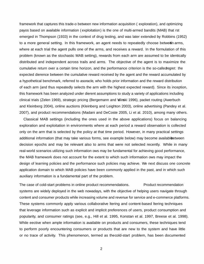
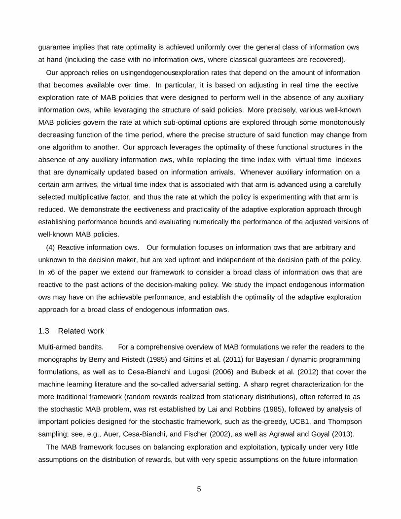
for some suitably selected δ. The general idea of adapting the exploration rate of a policy by advancing

17

t

Virtual time τ

Informationarrivals

MultiplicativeaccelerationMultiplicativeaccelerationMultiplicativeacceleration

t

Exploration rate f(τ) = 1/τ

Informationarrivals

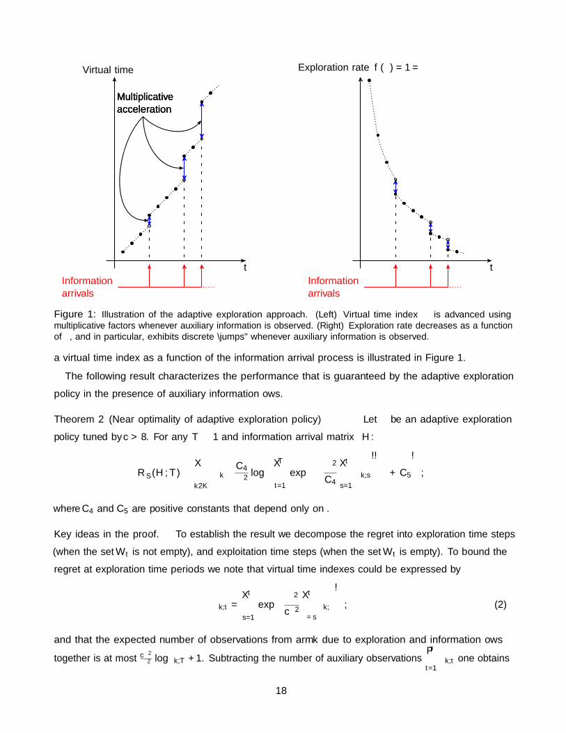
Figure 1: Illustration of the adaptive exploration approach. (Left) Virtual time index τ is advanced usingmultiplicative factors whenever auxiliary information is observed. (Right) Exploration rate decreases as a functionof τ , and in particular, exhibits discrete “jumps” whenever auxiliary information is observed.

a virtual time index as a function of the information arrival process is illustrated in Figure 1.

The following result characterizes the performance that is guaranteed by the adaptive exploration

policy in the presence of auxiliary information flows.

Theorem 2 (Near optimality of adaptive exploration policy) Let π be an adaptive exploration

policy tuned by c > 8. For any T ≥ 1 and information arrival matrix H:

RπS(H, T ) ≤∑k∈K

∆k

(C4

∆2log

(T∑t=1

exp

(−∆2

C4

t∑s=1

ηk,s

))+ C5

),

where C4 and C5 are positive constants that depend only on σ.

Key ideas in the proof. To establish the result we decompose the regret into exploration time steps

(when the set Wt is not empty), and exploitation time steps (when the set Wt is empty). To bound the

regret at exploration time periods we note that virtual time indexes could be expressed by

τk,t =

t∑s=1

exp

(∆2

cσ2

t∑τ=s

ηk,τ

), (2)

and that the expected number of observations from arm k due to exploration and information flows

together is at most cσ2

∆2 log τk,T + 1. Subtracting the number of auxiliary observationsT∑t=1

ηk,t one obtains

18

the first term in the upper bound. To analyze regret at exploitation time periods we use Chernoff-

Hoeffding inequality to bound the probability that a sub-optimal arm would have the highest estimated

reward, given the minimal number of observations that must be collected on each arm.

The upper bound in Theorem 2 holds for any arbitrary sample path of information arrivals that is

captured by the matrix H, and matches the lower bound in Theorem 1 with respect to dependence

on the sample path of information arrivals ηk,t’s, as well as the time horizon T , the number of arms

K, and the minimum expected reward difference ∆. This establishes a minimax regret rate of orderK∑k

log

(T∑t=1

exp

(−c ·

t∑s=1

ηk,s

))for the MAB problem with information flows that is formulated here,

where c is a constant that may depend on problem parameters such as K, ∆, and σ. Theorem 2

also implies that the adaptive exploration policy guarantees the best achievable regret (up to some

multiplicative constant) under any arbitrary sample path of information arrivals. Notably, the optimality

of the adaptive exploration policy applies to each of the settings that are described in §3.1, and matches

the lower bounds that were established in §3.1.1 and §3.1.2 for any parametric values of λ and κ.

Corollary 1 (Near optimality under stationary information flows) Let π be an adaptive explo-

ration policy with c > 8. If ηk,t’s are i.i.d. Bernoulli random variables with parameter λ then, for every

T ≥ 1:

EH [RπS(H, T )] ≤

(∑k∈K

∆k

)(cσ2

∆2log

(min

{T + 1,

cσ2 + 10∆2

∆2λ

})+ C

),

for some absolute constant C.

Corollary 2 (Near optimality under diminishing information flows) Let π be an adaptive explo-

ration policy with c > 8. If ηk,t’s are random variables such that for some κ ∈ R+, E [ηk,s] = d σsκ2∆2 log te

for each arm k ∈ K at each time step t, then for every T ≥ 1:

EH [RπS(H, T )] ≤

(∑k∈K

∆k

)cσ2

∆2log

2 +T 1− κ

4c − 1

1− κ4c

+T 1− κσ2

20∆2 − 1

1− κσ2

20∆2

+ C

,

for some absolute constant C.

While the adaptive exploration policy can be used for achieving near optimal performance, it serves us

mainly as a tool to communicate a broad approach for designing rate-optimal policies in the presence of

unknown information flows: adjusting policies that are designed to achieve “good” performance in the

absence of information flows, by endogenizing their exploration rates through virtual time indexes that

are advanced whenever new information is revealed. Notably, the approach of regulating exploration

rates based on realized information flows through advancing virtual time indexes (as specified in equation

(1) and illustrated in Figure 1) can be applied quite broadly over various algorithmic approaches. In

19

the following section we demonstrate that rate-optimal performance may be achieved by applying this

approach to known MAB policies that are rate optimal in the absence of auxiliary information flows.

5 Adjusting practical MAB policies

In §4 we introduced an approach to design efficient policies in the presence of auxiliary information by

regulating the exploration rate of the policy using a virtual time index, and by advancing that virtual

time through a properly selected multiplicative factor whenever auxiliary information is observed. To

demonstrate the practicality of this approach, we next apply it to adjust the design of the ε-greedy and

UCB1 policies, that were shown to achieve rate-optimal performance in the classical MAB framework.

5.1 ε-greedy with adaptive exploration

Consider the following adaptation of the ε-greedy policy (Auer et al. 2002).

ε-greedy with adaptive exploration. Input: a tuning parameter c > 0.

1. Initialization: set initial virtual times τk,0 = 0 for all k ∈ K

2. At each period t = 1, 2, . . . , T :

(a) Observe the vectors ηt, and Zt

(b) Update the virtual time steps for all k ∈ K:

τk,t =

τk,t−1 + 1 if t <

⌈Kcσ2

∆2

⌉(τk,t−1 + 1) · exp

(t∑

s=1

ηk,s∆2

cσ2

)if t =

⌈Kcσ2

∆2

⌉(τk,t−1 + 1) · exp

(ηk,t∆

2

cσ2

)if t >

⌈Kcσ2

∆2

⌉

(c) With probability min

{cσ2

∆2

K∑k′=1

1τk′,t

, 1

}select an arm at random: (exploration)

πt = k with probability

1τk,t

K∑k′=1

1τk′,t

, for all k ∈ K

Otherwise, select an arm with the highest estimated reward: (exploitation)

πt = arg maxk∈K

Xk,nk,t ,

(d) Receive and observe a reward Xπt,t

20

The ε-greedy with adaptive exploration policy chooses arms uniformly at random (explores) up to time

step t∗ =⌈Kcσ2

∆2

⌉. Then, at period t∗ the policy advances the virtual time indexes associated with the

different arms according to all the auxiliary information that has arrived up to time t∗. From period t∗+1

and on, the policy advances the virtual time indexes based on auxiliary information that has arrived

since the last period. Finally, at each step t > t∗, the policy explores with probability that is proportional

toK∑k′=1

τ−1k′,t, and otherwise pulls the arm with the highest empirical mean reward. In exploration periods,

arm k is explored with a probability that is weighted by τ−1k,t , based on the virtual time index that is

associated with that arm. Notably, in the ε-greedy with adaptive exploration policy virtual time indexes

are advanced in the same manner that was detailed in §4 in the description of the adaptive exploration

policy, except for an initial phase when for simplicity of analysis these indexes are set equal to the

time index t. The following result characterizes the guaranteed performance and establishes the rate

optimality of ε-greedy with adaptive exploration in the presence of unknown information flows.

Theorem 3 (Near optimality of ε-greedy with adaptive exploration) Let π be an ε-greedy with

adaptive exploration policy tuned by c > max{

16, 10∆2

σ2

}. Then, there exists a time index t∗ such that

for every T ≥ t∗, and for any information arrival matrix H, one has:


∆k

(C6

∆2log

(T∑

t=t∗+1

exp

(−∆2

C6

t∑s=1

ηk,τ

))+ C7

),

where C6, and C7 are positive constants that depend only on σ.

Key ideas in the proof. The proof of Theorem 3 follows ideas that are similar to the ones described

in the proof of Theorem 2, applying them to adjust the analysis of ε-greedy policy in Auer et al. (2002).

We decompose overall regret into exploration and exploitation time periods. To bound the regret at

exploration time periods, we express the virtual times similarly to (2). Letting tm denote the time

step at which the mth auxiliary observation for arm k realizes. We establish an upper bound on the

expected number of exploration time periods for arm k in the time interval [tm, tm+1 − 1], which scales

linearly with cσ2

∆2 log(τk,tm+1

τk,tm

)− 1. Summing over all possible values of m, we obtain that the regret

over exploration time periods is bounded from above by

∑k∈K

∆k ·cσ2

∆2log

(e

t∗ − 1/2

T∑t=t∗+1

exp

(−∆2

cσ2

t∑s=1

ηk,τ

)+ e

).

To analyze regret over exploitation time periods we first lower bound the number of observations

of each arm using Bernstein inequality, and then apply Chernoff-Hoeffding inequality to bound the

probability that a sub-optimal arm would have the highest estimated reward, given the minimal number

21

of observations on each arm. This regret component is constant term whenever c > max{

16, 10∆2

σ2

}.

5.2 UCB1 with adaptive exploration

Consider the following adaptation of the UCB1 policy (Auer et al. 2002).

UCB1 with adaptive exploration. Inputs: a tuning constant c, and estimated reward differ-

ences{

∆k

}k∈K

.

1. Initialization: set initial virtual times τk,0 = 0 for all k ∈ K

2. At each period t = 1, . . . , T :

(a) Observe the vectors ηt, and Zt

(b) Update the virtual times: τk,t = (τk,t−1 + 1) · exp

(ηk,t∆

2k

4cσ2

)for all k ∈ K

(c) Select the arm

πt =

t if t ≤ K

arg maxk∈K

{Xk,nk,t +

√cσ2 log τk,t

nk,t

}if t > K

(d) Receive and observe a reward Xπt,t

The UCB1 with adaptive exploration policy takes actions using the upper-confidence bounds Xk,nk,t +√cσ2 log τk,t

nk,t, where virtual time indexes τk,t are advanced multiplicatively (using the parameters {∆k})

whenever new information is realized. Notably, even though there are no explicit exploration periods in

UCB1, in the absence of auxiliary information flows this policy selects suboptimal actions at rate 1/t, and

therefore essentially explores at the same rate. Therefore, virtual times indexes is advanced essentially

as in previously discussed policies that explicitly explores at rate 1/t. The following result establishes

the rate optimality of UCB1 with adaptive exploration in the presence of unknown information flows.

Theorem 4 Let π be the adaptive UCB1 algorithm run with ∆k = ∆ for all k ∈ K. Then, for any

T ≥ 1, K ≥ 2, and auxiliary information arrival matrix H:


∆k

(C8

∆2log

(T∑t=1

exp

(−∆2

C8

t−1∑s=1

ηk,s

))+ C9

),

where C8, and C9 are positive constants that depend only on σ.

Key ideas in the proof. The proof adjusts the analysis of original UCB1 policy. Pulling a suboptimal

arm k at time step t implies at least one of the following three possibilities: (i) the empirical average of

22

the best arm deviates from its mean; (ii) the empirical mean of arm k deviates from its mean; or (iii)

arm k has not been pulled sufficiently often in the sense that

nk,t−1 ≤ lk,t −t∑

s=1

ηk,s,

where lk,t =4cσ2 log(τk,t)

∆2k

and nk,t−1 is the number of times arm k is pulled up to time t. The probability

of the first two events can be bounded using Chernoff-Hoeffding inequality, and the probability of the

third one can be bounded using:

T∑t=1

1

{πt = k, nk,t−1 ≤ lk,t −

t∑s=1

ηk,s

}≤ max

1≤t≤T

{lk,t −

t∑s=1

ηk,s

}.

Therefore, we establish that for any ∆k ≤ ∆k, one has

RπS(H, T ) ≤∑

k∈K\{k∗}

∆k

(C8

∆2k

· max1≤t≤T

log

(t∑

m=1

exp

(∆2k

C8

t∑s=m

ηk,s −∆2k

C8

t∑s=1

ηk,s

))+ C9,

).

plugging in ∆k = ∆, the result follows.

5.3 Numerical analysis

To demonstrate the practical value of the adaptive exploration approach and the validity of the

performance bounds that were established in the previous sections we analyze the empirical performance

policies in the presence of unknown information flows.

Setup. For each of the three reward distribution profiles that are listed in Table 1 (capturing three

levels of problem “hardness”), we considered three information arrival processes: stationary information

flows with ηk,t’s being i.i.d. Bernoulli random variables with mean λ = 500/T ; diminishing information

flows wheret∑

s=1ηk,t = b4

t c for each time period t and for each arm k; and no auxiliary information flows,

a basic setting that is used as a benchmark for the former two cases. We experimented with the three

policies that have been discussed in the previous sections: Adaptive exploration, ε-greedy with adaptive

exploration, and UCB1 with adaptive exploration, with a variety of tuning parameters. For each of the

reward profiles in Table 1 we tracked the average empirical regretT∑t=1

(µ∗ − µπt), that is, the average

performance difference between the best arm and the policy, over a decision horizon of T = 106 periods.

Averaging over 100 repetitions the outcome approximates the expected regret.

Results and discussion. Plots comparing the regret accumulation of the various algorithms for the

three different reward profiles appear in Figures 2, 3, and 4, and least squares estimation of the linear

23

Profile Mean rewards of different arms

1 0.9 0.8 0.8 0.8 0.8 0.8 0.8 0.8 0.8 0.82 0.9 0.8 0.8 0.8 0.7 0.7 0.7 0.6 0.6 0.63 0.9 0.6 0.6 0.6 0.6 0.6 0.6 0.6 0.6 0.6

Table 1: Three profiles of mean rewards, each includes mean rewards of 10 arms

approximations of these plots in the interval 105 ≤ t ≤ 106 are presented in Tables 2, 3, and 4. The

standard error of the estimated linear approximations are all smaller than 10−5. The presented results

were established using a tuning parameter of c = 0.2 for all three policies; we note that different

parametric values lead to similar results.5

No auxiliary Diminishing StationaryPolicy information flows information flows information flows

slope intercept slope intercept slope intercept

Adaptive exploration 17.98 0.59 14.65 4.19 0.26 187.85

Adaptive ε-greedy 17.92 −69.43 14.42 −60.02 0.25 124.36

Adaptive UCB1 20.72 −63.67 18.84 −68.62 3.92 131.41

Table 2: Slope and intercept estimates for profile 1




Adaptive ε-greedy 35.79 −144.01 29.03 −142.81 0.53 224.55

Adaptive UCB1 12.69 −30.51 7.37 −15.56 1.17 96.25





Adaptive ε-greedy 5.88 −2.51 2.58 0.95 0.00 54.73

Adaptive UCB1 6.58 −8.30 3.75 −3.91 0.00 59.91


Comparing the results under diminishing information flows with those without any auxiliary informa-

tion flows verifies the analysis in §3.1.2. One may observe that diminishing information flows lead to

5A selection of c = 0.2 achieved the best performance in the case without auxiliary information flows, and in thatsense this selection guarantees no loss relative to the best empirical tuning of the adjusted policies in the case withoutinformation flows. While achieving good performance, the value c = 0.2 does not belong to the range of parametric valuesfor which the theoretical performance bounds were established. This is aligned with observations in the MAB literaturewhere performance of tuning parameters belonging to a parametric region performance guarantees is dominated by theperformance of some parametric values that do not belong to this region; see, e.g., related discussions in Auer et al. (2002).

24

100 102 104 1060

50

100

150

200

250

100 102 104 1060

50

100

150

200

250

100 102 104 1060

50

100

150

200

250

Figure 2: Comparing regret accumulation for profile 1. (Left) no auxiliary information flows; (Middle) diminishinginformation flows; (Right) stationary information flows

100 102 104 1060

50

100

150

200

250

300

350

400

450

500

100 102 104 1060

50

100

150

200

250

300

350

400

450

500

100 102 104 1060

50

100

150

200

250

300

350

400

450

500


lower accumulated regret, but the rate of regret is logarithmic rather than constant since information

arrivals are not sufficiently frequent. Comparing the results with stationary information flows to those

without any auxiliary information flow validates the analysis in §3.1.1, demonstrating that if the rate

of information arrival, λ, is sufficiently high then the cumulative regret will be bounded from above

by a constant that depends on the information arrival rate λ. More precisely, we observe that for the

stationary information flows, the regret of the adaptive policies asymptotically converge to a constant

that is independent of T .

In addition to validating performance bounds, the results demonstrate the practical value that may

be captured by following the adjusted exploration approach in the presence of unknown information

flows. Our performance bounds show that by appropriately utilizing available information flows that are

sufficiently rich, one may reduce regret rates to a constant that is independent of T (as is apparent from

observing the left sides of Figures 2, 3, and 4 as well as observing the slope estimates in Tables 2, 3, and

4 for the stationary information flows). However, even when information flows are not rich enough to

25

100 102 104 1060

10

20

30

40

50

60

70

80

90

100 102 104 1060

10

20

30

40

50

60

70

80

90

100 102 104 1060

10

20

30

40

50

60

70

80

90


allow reduced regret rates, utilizing this information may have big impact on the empirical performance

in terms of reducing the accumulated regret and the multiplicative constant in the regret (as is apparent

from comparing accumulated regret values and the reduced slopes in the middle parts relative to the left

parts of Figures 2, 3, and 4, as well as comparing the values in Tables 2, 3, and 4, for the respective

information flows). Such regret reduction is very valuable in addressing many practical problems for

which MAB policies have been applied.

6 Reactive information flows

So far we have analyzed the performance of policies when information arrival processes are unknown,

but fixed. In particular, information flows were assumed to be independent of the decision trajectory of

the policy. In this section, we address some potential implications of endogenous information flows by

considering a simple extension of our model in which information flows depend on the past decisions of

the policy. For the sake of concreteness, we assume that the information flow on each arm is polynomially

proportional (decreasing or increasing) to the number of times various arms were selected. For some

global parameters γ > 0 and ω ≥ 0 that are fixed over arms and time periods, we assume that for each

time step t and arm k, the number of auxiliary observations received up to time t on arm k can be

described as follows:t∑

s=1

ηk,s =

ρk · nωk,t−1 +∑

j∈K\{k}

αk,jnγj,t−1

, (3)

where nk,t =t∑

s=11{πs = k} is the number of times arm k is selected up to time t, ρk ≥ 0 captures the

dependence of auxiliary observations of arm k on the past selections of arm k, and for each j 6= k the

parameter αk,j ≥ 0 capture the dependence of auxiliary observations of arm k on the past selections

of arm j. We assume that there exist non-negative values ρ, ρ, α, and α such that ρ ≤ ρk ≤ ρ and

26

α ≤ αk,j ≤ α for all arms k, j in K.

While the structure of (3) introduces some limitation on the impact the decision path of the policy

may have on the information flows, it still captures many types of dependencies. For example, when

γ = 0, information arrivals are decoupled across arms, in the sense that selecting an action at a given

period can impact only future information on that action. On the other hand, When γ > 0 a selection of

a certain action may impact future information arrivals on all actions.

A key driver in the regret complexity of this MAB formulation with endogenous information flows is

the order of the total number of times an arm is observed, nk,t = nk,t−1 +t∑

s=1ηk,t, relative to the order

of the number of times that arm is pulled, nk,t−1. Therefore, a first observation is that as long as nk,t

and nk,t−1 are of the same order, one recovers the classical regret rates that appear in the stationary

MAB literature; in particular, this is the case whenever ω < 1. Therefore, in the rest of this section we

focus on the case of ω ≥ 1.

A second observation is that when pulling an arm increases information arrival rates to other arms

(that is, whenever γ > 0 and α > 0), constant regret is achievable, and a myopic policy can guarantee

rate-optimal performance. This observation is formalized by the following proposition.

Proposition 1 Let π be a myopic policy that for the first K periods pulls each arm once, and at each

later period pulls the arm with the highest estimated mean reward, while randomizing to break ties.

Assume that α > 0 and γ > 0. Then, for any horizon length T ≥ 1 and for any history-dependent

information arrival matrix H such that (3) holds, one has

RπS(H, T ) ≤∑

k∈K\{k∗}

C10 · Γ( 1γ )

γ∆2γ−1

k

,

where Γ(·) is the gamma function, γ = min{γ, 1}, and C10 > 0 is a constant that depends on α.

We next turn to characterize the case in which information flows are decoupled across arms, in the

sense that selecting a certain arm does not impact information flows associated with other arms. To

evaluate the performance of the adaptive exploration approach under this class of reactive information

flows we use the adaptive exploration policy given in §4. We note that the adjusted policies presented in

§5 could be shown to maintain similar performance guarantees.

Theorem 5 (Near Optimality under decoupled endogenous information flows) Assume that

γ = 0 and ω ≥ 1. Then:

(i) For any T ≥ 1 and history-dependent information arrival matrix H that satisfies (3), the regret

27

incurred by any admissible policy π ∈ P, is bounded below as follows

RπS(H, T ) ≥ C11K

ρ∆2ω−1

(log (T/K))1/ω ,

for some positive constant C11 > 0 that depends on σ.

(ii) Let π be the adaptive exploration policy (detailed in §4), tuned by c > 8. Then, for any T ≥⌈

4cKσ2

∆2

⌉RπS(H, T ) ≤ C12 · (log T )1/ω ·

∑k∈K\{k∗}

1

ρ∆2ω−1

k

+∑

k∈K\{k∗}

C13∆k,

where C12, and C13 are positive constants that depend on σ and c.

Theorem 5 introduces matching lower and upper bounds that establish optimality under the class of

decoupled endogenous information flows defined by (3) with γ = 0 and ω ≥ 1. For example, Theorem 5

implies that under our class of reactive information flows, whenever mean rewards are separated (that is,

for each k one has that ∆k is independent of T ), the best achievable performance is a regret is of order

(log T )1/ω.

Key ideas in the proof. The first part of the result is derived by replacing the sum∑t

s=1 ηk,s by

its upper bound, ρnωk,t−1, and following the proof of Theorem 1. To establish the second part of the

result, we rely on the proof of Theorem 2 and perform a worst-case analysis for the part of the regret

that is caused by exploration. We show that in this case, the jth exploration of arm k are separated by

cσ2

∆2 τk,tk,j time periods from other explorations of that arm, where tk,j is the time step at which the jth

exploration of arm k took place. The result is then obtained by plugging (3) into the expression of τk,t

and observing that tk,j − tk,j−1 ≤ T for all possible j.

Notably, in proving the second part of Theorem 5 we assume no prior knowledge of either the class of

information arrival processes given by (3), or the parametric values under this structure. Therefore, the

adaptive exploration policy is agnostic to the structure of the information flows.

7 Concluding remarks

Summary of results. In this paper we considered a generalization of the stationary multi-armed

bandits problem in the presence of unknown and arbitral information flows on each arm. We studied the

impact of such auxiliary information on the design of efficient learning policies and on the performance

that can be achieved. In particular, we studied the design of learning policies that adapt in real time to

the unknown information arrival process. We introduced a general approach of adjusting existing MAB

policies that are designed to perform well in the absence of auxiliary information flows by controlling

28

the exploration rate that is governed by the policy through advancing a virtual time indexes that are

customized for each arm every time information on this arm arrives. We established that using this

approach one may guarantee the best performance (in terms of minimax regret) that is achievable under

prior knowledge on the information arrival process, and demonstrated through performance bounds as

well as empirical experiments the effectiveness of this approach in adapting “of the shelf” MAB polices.

Inseparable mean rewards. As mentioned in §2.1, all our results hold also when ∆, the lower bound

on the minimum difference of expected rewards relative to the best arm, is allowed to scale with T , and

in particular, to decrease with T . When ∆ is of order T−1/2, this leads to a spectrum of minimax regret

rates, from order T 1/2 in the absence of information flows (coinciding with the worst case of inseparable

mean rewards in the classical stochastic MAB framework), and constant regret that is independent of T .

Avenues for future research. As mentioned in §2, our results hold when there exists some invertible

mapping φ such that the auxiliary information Y has the same distribution as φ(X). One interesting

direction for future research is to study cases where the mapping φ is a priori unknown; such case may

require more sophisticated estimation of mean rewards relative to the empirical mean that was used

in this paper. One possible approach for addressing this challenging problem might be to estimate

the mapping φ throughout some initial period, form an estimated inverse mapping φ−1, and only then

leverage auxiliary information flows for improving the estimators of the mean rewards.

In §6 we considered information flows that are allowed to be reactive to the history of decisions

and observations, and established that optimality of our approach for a class of such information

flows. Nevertheless, the characterization of minimax regret rates and optimal policy design for general

endogenous information flows is a challenging open problem.

29

A Proofs of Main results

A.1 Preliminaries

In all the following proofs, we will have the following notations: Let nk,t be the number of times arm k

is pulled by the policy up to time t (the time steps that the output of the arm is observed due to free

information arrival are excluded):

nk,t =t∑

s=1

1{πs = k}.

Let nk,t be the number of samples observed from arm k up to time t:

nk,t = nk,t−1 +

t∑s=1

ηk,s.

Denote by Xk,nk,t the empirical average of the kth arm reward after nk,t observations:

Xk,nk,t =

ηk,tYk,t +t−1∑s=1

(ηk,sYk,s + 1{πs = k}Xk,s)

nk,t.

For any policy π, and profile ν, let Pπν , Eπν , and Rπν denote the probability, expectation, and regret when

the arm rewards are distributed according to ν.

A.2 Proof of Theorem 1

Step 1 (Notations and definitions). We define the distribution profiles ν(m,q) withm, q ∈ {1, . . . ,K}

as follows:

ν(m,q)k =

N (0, σ2) if k = m

N (+∆, σ2) if k = q 6= m

N (−∆, σ2) o.w.

.

For example one has that,

ν(1,1) =

N (0, σ2)

N (−∆, σ2)

N (−∆, σ2)...

N (−∆, σ2)

, ν(1,2) =

N (0, σ2)

N (+∆, σ2)

N (−∆, σ2)...

N (−∆, σ2)

, ν(1,3) =

N (0, σ2)

N (−∆, σ2)

N (+∆, σ2)...

N (−∆, σ2)

, . . . , ν(1,K) =

N (0, σ2)

N (−∆, σ2)

N (−∆, σ2)...

N (+∆, σ2)

.

30

Step 2 (Lower bound decomposition). We note that

RπS(H, T ) ≥ maxm,q∈{1,...,K}

{Rπν(m,q)(H, T )

}≥ 1

K

K∑m=1

maxq∈{1,...,K}

{Rπν(m,q)(H, T )

}. (4)

Step 3 (A naive lower bound for maxq∈{1,...,K}

{Rπν(m,q)(H, T )}). We note that

maxq∈{1,...,K}

{Rπν(m,q)(H, T )} ≥ Rπ

ν(m,m)(H, T ) = ∆ ·∑

k∈K\{m}

Eν(m,m) [nk,T ]. (5)

Step 4 (An information theoretic lower bound). For any profile ν, denote by νt the distribution

of the observed rewards up to time t under ν. By Lemma 2, for any q 6= m, one has

KL(ν(m,m)t ,ν

(m,q)t ) =

2∆2

σ2· Eν(m,m) [nq,t] =

2∆2

σ2

(Eν(m,m) [nq,t−1] +

t∑s=1

ηq,s

). (6)

One obtains:

maxq∈{1,...,K}

{Rπν(m,q)(H, T )} ≥ 1

KRπν(m,m)(H, T ) +

1

K

∑q∈K\{m}

Rπν(m,q)(H, T )

≥ ∆

K

T∑t=1

∑k∈K\{m}

Pν(m,m){πt = k}+∆

K

∑q∈K\{m}

T∑t=1

Pν(m,q){πt = m}

=∆

K

T∑t=1

∑q∈K\{m}

(Pν(m,m){πt = q}+ Pν(m,q){πt = m})

(a)

≥ ∆

2K

T∑t=1

∑q∈K\{m}

exp(−KL(ν(m,m)t ,ν

(m,q)t ))

(b)=

∆

2K

T∑t=1

∑q∈K\{m}

exp

[−2∆2

σ2

(Eν(m,m) [nq,t−1] +

t∑s=1

ηq,s

)](c)

≥ ∆

2K

T∑t=1

∑q∈K\{m}

exp

[−2∆2

σ2

(Eν(m,m) [nq,T ] +

t∑s=1

ηq,s

)]

=∑

q∈K\{m}

∆ · exp(−2∆2

σ2 · Eν(m,m) [nq,T ])

2K

T∑t=1

exp

(−2∆2

σ2

t∑s=1

ηq,s

), (7)

where (a) follows from Lemma 1, (b) holds by (6), and (c) follows from nq,T ≥ nq,t−1 for t ∈ T .

31

Step 5 (Unifying the lower bounds in steps 3 and 4). Using (5), and (7), we establish:

maxq∈{1,...,K}

{Rπν(m,q)(H, T )} ≥ ∆

2

∑k∈K\{m}

Eν(m,m) [nk,T ] +exp

(−2∆2

σ2 · Eν(m,m) [nk,T ])

2K

T∑t=1

exp

(−2∆2

σ2

t∑s=1

ηk,s

)≥ ∆

2

∑k∈K\{m}

minx>0

x+exp

(−2∆2

σ2 · x)

2K

T∑t=1

exp

(−2∆2

σ2

t∑s=1

ηk,s

)(a)

≥ σ2

4∆

∑k∈K\{m}

log

(∆2

σ2K

T∑t=1

exp

(−2∆2

σ2

t∑s=1

ηk,s

)), (8)

where (a) follows from x+ γe−κx ≥ log γκκ for γ, κ, x > 0. (Note that the function x+ γe−κx ≥ log γκ

κ is a

convex function and we can find its minimum by taking its derivative and putting it equal to zero.) The

result is then established by putting together (4), and (8).


Step 1 (Decomposing the regret). Fix T ≥ 1, K ≥ 2, and H ∈ {0, 1}K×T , and profile ν. For

simplicity of notation, define events Ek,t that at time t, and for arm k we have

nk,t ≥cσ2

∆2log (τk,t) .

In words, this event means at time t the policy has seen arm k an enough number of times and will

not perform exploration on this arm at this time step. Let π be the Adaptive-exploration policy. We

decompose the regret of a suboptimal arm k 6= k∗:

∆k · Eπν

[T∑t=1

1 {πt = k}

]≤ ∆k ·

Jk,1︷︸︸︷Eπν

[T∑t=1

1

{k = arg min

j∈Wt

nj,t ∧ Ek,t}]

+ ∆k · Eπν

[T∑t=1

1

{k = arg max

j∈KXj,nk,t ∧ ∩j∈KEj,t

}]︸︷︷︸

Jk,2

, (9)

where Ek,t is the complement of Ek,t. The component Jk,1 is the expected number of times arm k is

pulled due to exploration, while the the component Jk,2 is the one due to exploitation.

32

Step 2 (Analysis of τk,t). We will later find upper bounds for the quantities Jk,1, and Jk,2 that are

functions of the virtual time τk,T . A simple induction results in the following expression:

τk,t =t∑

s=1

exp

(∆2

cσ2

t∑τ=s

ηk,τ

). (10)

Step 3 (Analysis of Jk,1). Define

Ek,t = ηk,t +t−1∑s=1

(ηk,s + 1

{k = arg min

j∈Ws

nj,s ∧ Ek,s})

. (11)

By induction, we next show that for t = 1, . . . , T + 1:

Ek,t ≤cσ2

∆2log (τk,t) + 1. (12)

The base case is

Ek,1 = ηk,1 =cσ2

∆2log

(exp

(∆2

cσ2ηk,1

))=cσ2

∆2log (τk,1) ≤ cσ2

∆2log (τk,1) + 1.

Assume that (12) holds for all s ≤ t. To establish that it also holds for t+ 1, we will show that

Ek,t+1 ≤cσ2

∆2log (τk,t) + 1 + ηk,t+1. (13)

We consider two cases. In the first one, 1{k = arg minj∈Ws nj,s ∧ Ek,s

}= 0. As a result, we have

Ek,t+1 = Ek,t + ηk,t+1 ≤cσ2

∆2log (τk,t) + 1 + ηk,t+1.

In the second case, 1{k = arg minj∈Wt nj,t ∧ Ek,t

}= 1. This impliesEk,t ≤ nk,t <

cσ2

∆2 log (τk,t). There-

fore,

Ek,t+1 = Ek,t + ηk,t+1 + 1 ≤ cσ2

∆2log (τk,t) + 1 + ηk,t+1,

and therefore (13) is established. The following inequality completes the induction:

cσ2

∆2log (τk,t) + 1 + ηk,t+1 =

cσ2

∆2log

(τk,t · exp

(∆2

cσ2ηk,t+1

))+ 1 ≤ cσ2

∆2log (τk,t+1) + 1.

33

Therefore, one obtains:

Jk,1(a)= Eπν [Ek,T+1]−

T∑t=1

ηk,t

(b)

≤ cσ2

∆2log (τk,T+1) + 1−

T∑t=1

ηk,t

=cσ2

∆2log (τk,T+1) + 1 +

cσ2

∆2log

(exp

(−∆2

cσ2

T∑t=1

ηk,t

))(c)

≤ cσ2

∆2log

(1 +

T∑t=1

exp

(−∆2

cσ2

t∑s=1

ηk,τ

))+ 1, (14)

where (a) and (b) follow from (11) and (12) respectively, and (c) holds by replacing τk,T+1 with the

expression in (10).

Step 4 (Analysis of Jk,2). We note that:

Jk,2 ≤T∑t=1

P{Xk,nk,t > Xk∗,nk∗,t ∧ Ek,t

}. (15)

We upper bound each summand as follows:

P{Xk,nk,t > Xk∗,nk,t ∧ Ek,t

}≤ P

{Xk,nk,t > µk +

∆k

2∧ Ek,t

}+ P

{Xk∗,nk∗,t < µk∗ +

∆k

2∧ Ek,t

}. (16)

We next upper bound the first term on the right-hand side of the above inequality; the second term can

be treated similarly. Now, one obtains:

P{Xk,nk,t > µk +

∆k

2∧ Ek,t

}(a)

≤ P{Xk,nk,t > µk +

∆k

2| Ek,t

}(b)

≤ exp

(−∆2

kc

8∆2log τk,t

)≤ 1

(τk,t)c/8

(c)

≤ 1

tc/8, (17)

where (a) holds by the conditional probability definition, (b) follows from Lemma 3, and the fact that

nk,t ≥ nk,t, and (c) is a result of (10). The results is then established by putting together (9), (14), (15),

(16), and (40). This concludes the proof.

34

A.4 Proof of Corollary 1

EH [RπS(H, T )](a)

≤ EH

[∑k∈K

cσ2∆k

∆2log

(T∑t=1

exp

(−∆2

cσ2

t∑s=1

ηk,s

))+ C∆k

](b)

≤∑k∈K

[cσ2∆k

∆2log

(EH

[T∑t=1

exp

(−∆2

cσ2

t∑s=1

ηk,s

)])+ C∆k

](c)

≤

(∑k∈K

∆k

)·

(cσ2

∆2log

(1− exp (−Tλ/10)

λ/10+

1− exp(−∆2Tλ/cσ2

)∆2λ/cσ2

)+ C

)

≤

(∑k∈K

∆k

)·(cσ2

∆2log

(1

λ/10+

1

∆2λ/cσ2

)+ C

), (18)

where: (a) holds by Theorem 2, (b) follows from Jensen’s inequality and the concavity of log(·), and (c)

holds by Lemmas 5 and 6. By noting thatT∑t=0

exp

(−∆2

cσ2

t∑s=1

ηk,s

)< T + 1, the result is established.

A.5 Proof of Corollary 2

EH [RπS(H, T )](a)

≤ EH

[∑k∈K

cσ2∆k

∆2log

(T∑t=1

exp

(−∆2

cσ2

t∑s=1

ηk,s

))+ C∆k

](b)

≤∑k∈K

[cσ2∆k

∆2log

(EH

[T∑t=1

exp

(−∆2

cσ2

t∑s=1

ηk,s

)])+ C∆k

](c)

≤

(∑k∈K

∆k

)·

(cσ2∆k

∆2log

(T∑t=1

exp

(−κ4c

log t

)+ exp

(−κσ2

20∆2log t

))+ C

)

=

(∑k∈K

∆k

)·

(cσ2∆k

∆2log

(T∑t=1

t−κ4c + t

−κσ2

20∆2

)+ C

)

≤

(∑k∈K

∆k

)·(cσ2∆k

∆2log

(2 +

∫ T

1

(t−κ4c + t

−κσ2

20∆2

)dt

)+ C

)

=

(∑k∈K

∆k

)·

cσ2∆k

∆2log

2 +T 1− κ

4c − 1

1− κ4c

+T 1− κσ2

20∆2 − 1

1− κσ2

20∆2

+ C

(19)

where: (a) holds by Theorem 2, (b) follows from Jensen’s inequality and the concavity of log(·), and (c)

holds by Lemma 5.


The structure of this proof is very similar to that of the proof of Theorem 2. Let t∗ = dKcσ2

∆2 e, and fix

T ≥ t∗, K ≥ 2, H ∈ {0, 1}K×T , and profile ν ∈ S.

35

Step 1 (Decomposing the regret). We decompose the regret of a suboptimal arm k 6= k∗:

∆k · Eπν

[T∑t=1

1 {πt = k}

]= ∆k ·

Jk,1︷︸︸︷Eπν

[T∑t=1

1 {πt = k, policy does exploration}

]

+ ∆k · Eπν

[T∑t=1

1 {πt = k, policy does exploitation}

]︸︷︷︸

Jk,2

. (20)

The component Jk,1 is the expected number of times arm k is pulled due to exploration, while the the

component Jk,2 is the one due to exploitation.

Step 2 (Analysis of τk,t). We will later find upper bounds for the quantities Jk,1, and Jk,2 that are

functions of the virtual time τk,T . Assume t ≥ t∗. A simple induction results in the following expression:

τk,t = t∗ exp

(∆2

cσ2

t∑τ=1

ηk,τ

)+

t∑s=t∗+1

exp

(∆2

cσ2

t∑τ=s

ηk,τ

). (21)

Step 3 (Analysis of Jk,1). Let M =T∑t=1

ηk,t, and M =t∗∑t=1

ηk,t. Let tm be the time step at which the

mth auxiliary observation for arm k is received, that is,

tm =

max

{t∗,min

{0 ≤ t ≤ T |

t∑s=1

ηk,s = m

}}if M ≤ m ≤ M

T + 1 if m = M + 1

.

36

Note that we dropped the index k in the definitions above for simplicity of notation. Also define

τk,T+1 = (τk,T + 1) · exp(ηk,t∆

2

cσ2

). One has:

Jk,1 =T∑t=1

min

{cσ2

∆2

K∑k′=1

1

τk′,t, 1

}·

1τk,t

K∑k′=1

1τk′,t

=t∗ − 1

K+

T∑t=t∗

cσ2

∆2τk,t

=t∗ − 1

K+

M∑m=M

tm+1−tm−1∑s=0

cσ2

∆2(τk,tm + s)

(a)

≤ t∗ − 1

K+

M∑m=M

cσ2

∆2log

(τk,tm + tm+1 − tm − 1 + 1/2

τk,tm − 1/2

)(b)

≤ t∗ − 1

K+

M∑m=M

cσ2

∆2log

exp(−∆2

cσ2

)·(τk,tm+1 − 1/2

)τk,tm − 1/2

=t∗ − 1

K+cσ2

∆2log

(τk,tM+1

− 1/2

τk,tM − 1/2

)−

T∑t=t∗+1

ηk,t

=t∗ − 1

K+cσ2

∆2log

(τk,T+1 − 1/2

τk,t∗ − 1/2

)−

T∑t=t∗+1

ηk,t

≤ t∗ − 1

K+cσ2

∆2log

(τk,T+1 − 1/2

t∗ − 1/2

)−

T∑t=1

ηk,t

(c)

≤ t∗ − 1

K+cσ2

∆2log

(1

t∗ − 1/2

T∑t=t∗+1

exp

(−∆2

cσ2

t∑s=1

ηk,τ

))+ 1

≤ cσ2

∆2log

(e

t∗ − 1/2

T∑t=t∗+1

exp

(−∆2

cσ2

t∑s=1

ηk,τ

))+ e, (22)

where (a), (b), and (c) follow from Lemma 7, the fact that exp(

∆2

cσ2

)(τk,tm + tm+1,k − tm) = τk,tm+1 ,

and (21), respectively.

Step 4 (Analysis of nk,t). To analyze Jk,2 we bound nk,t, the number of samples of arm k at each

time t such that t ≥ t∗. Fix t ≥ t∗. Then, nk,t is a summation of independent Bernoulli r.v.’s. One has

E [nk,t] =t∗ − 1

K+

t∑s=1

ηk,s +t−1∑s=t∗

cσ2

∆2τk,s. (23)

37

The termt−1∑s=t∗

cσ2

∆2τk,scan be bounded similar to Step 3. Let Mt =

t−1∑s=1

ηk,s and M =t∗∑s=1

ηk,s. Let tm,t be

the time step at which the mth auxiliary observation for arm k is received up to time t− 1, that is,

tm,t =

max

{t∗,min

{0 ≤ s ≤ T |

q∑s=1

ηk,q = m

}}if M ≤ m ≤ Mt

t− 1 if m = Mt + 1

.

One has that

t−1∑s=t∗

cσ2

∆2τk,s=

Mt∑m=M

tm+1,t−tm,t−1∑s=0

cσ2

∆2(τk,tm,t + s)

(a)

≥Mt∑

m=M

cσ2

∆2log

(τk,tm,t + tm+1,t − tm,t

τk,tm,t

)

=

Mt∑m=M

cσ2

∆2log

exp(−∆2

cσ2

)τk,tm+1,t

τk,tm,t

=cσ2

∆2log

(τk,t−1

τk,t∗

)−

t−1∑s=t∗+1

ηk,s

=cσ2

∆2log(τk,t−1

t∗

)−

t−1∑s=1

ηk,s, (24)

where (a) follows from Lemma 7. Putting together (23) and (24), one has

E [nk,t] ≥t∗ − 1

K+cσ2

∆2log(τk,t−1

t∗

)≥ −1

K+cσ2

∆2log(eτk,t−1

t∗

):= xt. (25)

Now by Lemma 4, we have

P{nk,t ≤

xt2

}≤ exp

(−xt10

)= exp

(−1

10K

)·(

t∗

eτk,t−1

)−cσ2

10∆2

≤ exp

(1

10K

)·(

t∗

e(t− 1)

)−cσ2

10∆2

, (26)

where the last inequality follows from (21).

Step 5 (Analysis of Jk,2). We note that:

Jk,2 ≤T∑t=t∗

P{Xk,nk,t > Xk∗,nk∗,t

}. (27)

38


P{Xk,nk,t > Xk∗,nk,t

}≤ P

{Xk,nk,t > µk +

∆k

2

}+ P

{Xk∗,nk∗,t < µk∗ +

∆k

2

}. (28)

We next bound the first term on the right-hand side of the above inequality; the second term can be

treated similarly. One obtains:

P{Xk,nk,t > µk +

∆k

2

}(a)

≤ P{Xk,nk,t > µk +

∆k

2| nk,t >

xt2

}+ P

{nk,t ≤

xt2

}(b)

≤ exp

(−∆2

kxt16σ2

)+ exp

(1

10K

)·(

t∗

e(t− 1)

)−cσ2

10∆2

≤ exp

(∆2k

16Kσ2

)· exp

(−c16

log(eτk,t−1

t∗

))+ exp

(1

10K

)·(

t∗

e(t− 1)

)−cσ2

10∆2

(c)

≤ exp

(∆2k

16Kσ2

)·(

t∗

e(t− 1)

)−c16

+ exp

(1

10K

)·(

t∗

e(t− 1)

)−cσ2

10∆2

, (29)

where: (a) holds by the conditional probability definition; (b) follows from Lemma 3 together with (26);

and (c) holds by (21). Putting together (20), (22), (27), (28), and (29), the result is established.


Fix a profile ν ∈ S and consider a suboptimal arm k 6= k∗. If arm k is pulled at time t, then

Xk,nk,t +

√cσ2 log τk,t

nk,t≥ Xk∗,nk∗,t +

√cσ2 log τk∗,t

nk∗,t.

Therefore, at least one of the following three events must occur:

E1,t =

{Xk,nk,t ≥ µk +

√cσ2 log τk,t

nk,t

}, E2,t =

{Xk∗,nk∗,t ≤ µk∗ −


nk∗,t

},

E3,t =

{∆k ≤ 2

√cσ2 log τk,t

nk,t

}.

To see why this is true, assume that all the above events fail then, we have

Xk,nk,t +

√cσ2 log τk,t

nk,t< µk + 2

√cσ2 log τk,t

nk,t< µk + ∆k = µk∗ < Xk∗,nk∗,t +


nk∗,t.

39

For any sequence {lk,t}t∈T , and {lk,t}t∈T , such that lk,t ≥ lk,t for all t ∈ T , we can see that

Eπν [nk,T ] = Eπν

[T∑t=1

1 {πt = k}

]= Eπν

[T∑t=1

1 {πt = k, nk,t ≤ lk,t}+ 1 {πt = k, nk,t > lk,t}

]

≤ Eπν

[T∑t=1

1

{πt = k, nk,t ≤ lk,t

}+ 1 {πt = k, nk,t > lk,t}

]

≤ Eπν

[T∑t=1

1

{πt = k, nk,t−1 ≤ lk,t −

t∑s=1

ηk,s

}]+

T∑t=1

P {πt = k, nk,t > lk,t}

≤ max1≤t≤T

{lk,t −

t∑s=1

ηk,s

}+

T∑t=1

P {πt = k, nk,t > lk,t} .

If we set

lk,t =4cσ2 log (τk,t)

∆2k

, and lk,t =4cσ2 log (τk,t)

∆2k

(30)

then, to have nk,t > lk,t, it must be the case that E3,t does not occur. Therefore,

Eπν [nk,T ] ≤ max1≤t≤T

{lk,t −

t∑s=1

ηk,s

}+

T∑t=1

P {πt = k,E3,t fails}

≤ max1≤t≤T

{lk,t −

t∑s=1

ηk,s

}+

T∑t=1

P {E1,t or E2,t}

≤ max1≤t≤T

{lk,t −

t∑s=1

ηk,s

}+

T∑t=1

2

τc/2k,t

, (31)

where the last inequality follows from Lemma 3, and union bound. Using an induction, one may obtain

that

τk,t =

t∑s=1

exp

(∆2k

4cσ2

t∑τ=s

ηk,τ

)≥ t. (32)

Plugging in this expression into (31), one obtains

Eπν [nk,T ] ≤ max1≤t≤T

{4cσ2

∆2k

log

(t∑

s=1

exp

(−∆2

k

4cσ2

s−1∑τ=1

ηk,τ

))}+

T∑t=1

2

τc/2k,t

=4cσ2

∆2k

log

(T∑t=1

exp

(−∆2

k

4cσ2

t−1∑s=1

ηk,s

))+

T∑t=1

2

τc/2k,t

≤ 4cσ2

∆2k

log

(T∑t=1

exp

(−∆2

k

4cσ2

t−1∑s=1

ηk,s

))+

T∑t=1

2

tc/2

Putting ∆k = ∆k concludes the proof.

40


First, we prove the lower bound.The first three steps of the proof of Theorem 1 holds for the new setting

as well. In step 4, equation (6) can be modified as follows:

KL(ν(m,m)t ,ν

(m,q)t ) =

2∆2

σ2·Eν(m,m) [nq,t] =

2∆2

σ2Eν(m,m)

[nq,t−1 +

t∑s=1

ηq,s

]≤ 2∆2

σ2Eν(m,m)

[(1 + ρ)nωq,t−1

],

(33)

where the last inequality follows from nωq,t−1 ≥ nq,t−1 for ω ≥ 1. Accordingly, (7) can be modified as well:

maxq∈{1,...,K}

{Rπν(m,q)(H, T )}

(a)

≥ ∆

2K

T∑t=1

∑q∈K\{m}

exp

(−2∆2(1 + ρ)

σ2Eν(m,m)

[nωq,t−1

])(b)

≥ ∆T

2K

∑q∈K\{m}

exp

(−2∆2(1 + ρ)

σ2Eν(m,m) [nωq,T ]

), (34)

where (a) follows from the steps in (7), and (33), and (b) holds by (33). Using (5), and (34), we establish:

maxq∈{1,...,K}

{Rπν(m,q)(H, T )} ≥ ∆

2

∑k∈K\{m}

(Eν(m,m) [nk,T ] +

T

2Kexp

(−2∆2(1 + ρ)

σ2Eν(m,m) [nωq,T ]

))

≥ ∆

2

∑k∈K\{m}

minx>0

(x+

T

2Kexp

(−2∆2(1 + ρ)

σ2xω))

(a)

≥ ∆(K − 1)

2

(σ2

2∆2(1 + ρ)ωlog

(Tω∆2(1 + ρ)ω

2ω−1Kωσ2

))1/ω

, (35)

where (a) follows from (x+ γe−κx)ω ≥ xω + γωe−κωx ≥ log(γωκω)

κω for γ, κ, x > 0, and ω ≥ 1. The lower

bound follows from putting (4), and (35) together.

Now, we analyze the regret of the adaptive exploration policy. Similar to the proof of the regret lower

bound, we will modify the proof of Theorem 2 to make it work for the setting of §6. Steps 1, 2, and 4 of

the mentioned proof hold for this setting as well. We will focus on adjusting step 3 in the proof, that is,

analyzing Jk,1. Define

Jk,1 :=

T∑t=1

1

{k = arg min

j∈Wt

nj,t ∧ Ek,t},

By the structure of the adaptive exploration policy, if t ≥ t∗ := 4cKσ2

∆2 then

nk,t ≥cσ2

∆2log (τk,t)−

t∑s=1

ηk,s.

41

Note that by the definition of τk,t’s, we have

cσ2

∆2log(τk,t)−

cσ2

∆2log(τk,t−1) =

cσ2

∆2log(1 +

1

τk,t−1) + ηk,t,

which implies

nk,t ≥cσ2

∆2log (τk,t)−

t∑s=1

ηk,s =t∑

s=2

cσ2

∆2log(1 +

1

τk,s−1). (36)

Let tk,j be the time step at which the jth exploration is performed on arm k. By the structure of the

policy, and (36), for tk,j ≥ t∗, we have

tk,j+1−1∑s=tk,j

cσ2

∆2log(1 +

1

τk,s−1) ≥ 1.

Note that τk,t is a decreasing sequence, which implies

tk,j+1 − tk,j ≥cσ2

∆2

log(1 + 1τk,tk,j−1

)

(a)

≥ cσ2

∆2τk,tk,j

(b)

≥ cσ2

∆2exp

(∆2(ρ(j − 1)ω − 1)

cσ2

), (37)

where (a) follows from log(1 + x) ≤ x for every x ≥ 1, and (b) follows from (10). Let j = Jk,1 in (37):

cσ2

∆2exp

(∆2(ρ(Jk,1 − 1)ω − 1)

cσ2

)≤ tk,Jk,1 − tk,Jk,1−1 ≤ T − t

∗ ≤ T,

which implies

Jk,1 ≤ 1 +

(1

ρ+cσ2

ρ∆2(2 + log T )

) 1ω

.

This concludes the proof.

A.9 Proof of Proposition 1

Define γ = min{1, γ}, and α = min{1, α}. First, we will show that for any arm k, and at any time step

t, we have

nk,t ≥ α(t− 1)γ . (38)

42

We will consider two cases. In the first one, assume γ ≥ 1 then, we will have

nk,t = nk,t−1 +t∑

s=1

ηk,s ≥ nk,t−1 +∑

j∈K\{k}

αnγj,t−1

≥ nk,t−1 +∑

j∈K\{k}

αnj,t−1

≥ min{1, α}K∑j=1

nj,t−1 = min{1, α}(t− 1) = α(t− 1)γ .

In the second case, assume γ < 1. One obtains

nk,t ≥ nk,t−1 +∑

j∈K\{k}

αnγj,t−1 ≥ nγk,t−1 +

∑j∈K\{k}

αnγj,t−1

≥ min{1, α}K∑j=1

nγj,t−1 = α(t− 1)γ ,

where the last step follows from the fact that xγ + yγ ≥ (x+ y)γ for x, y ≥ 0, and γ < 1.

In order to upper bound the regret, we will use the usual decomposition

Rπgreedy

S (H, T ) =T∑t=1

∑k∈K\{k∗}

∆kP {πt = k} .


P {πt = k} ≤ P{Xk,nk,t > Xk∗,nk,t

}≤ P

{Xk,nk,t > µk +

∆k

2

}+ P

{Xk∗,nk∗,t < µk∗ −

∆k

2

}. (39)

We next upper bound the first term on the right-hand side of the above inequality; the second term can

be treated similarly. Now, one obtains:

P{Xk,nk,t > µk +

∆k

2

}(a)

≤ E[exp

(−∆2

k

8σ2nk,t

)](b)

≤ exp

(−∆2

k

8σ2α(t− 1)γ

)(40)

where (a), and (b) hold by Lemma 3, and (38). Finally, note that

T∑t=1

P {πt = k} ≤T∑t=1

2 exp

(−∆2

k

8σ2α(t− 1)γ

)≤ 2 +

Γ( 1γ )

γ

(8σ2

∆2k

)1/γ

, (41)

where the last inequality follows form∞∑t=1

exp(−tγ) ≤Γ( 1γ

)

γ .

43

B Auxiliary Lemmas

Lemma 1 (Tsybakov 2008, Lemma 2.6) Let ρ0, ρ1 be two probability distributions supported on

some set X, with ρ0 absolutely continuous with respect to ρ1. Then for any measurable function

Ψ : X→ {0, 1}, one has:

Pρ0{Ψ(X) = 1}+ Pρ1{Ψ(X) = 0} ≥ 1

2exp(−KL(ρ0, ρ1)).

Lemma 2 (Gerchinovitz and Lattimore 2016, Lemma 1) Consider two profiles ν, and ν ′. De-

note by νt (ν ′t) the distribution of the observed rewards up to time t under ν (ν ′ respectively). Let

nk,t be the number of times a sample from arm k has been observed up to time t, that is nk,t =

ηk,t +t−1∑s=1

(ηk,s + 1{πs = k}). For any policy π, we have

KL(νt,ν′t) =

K∑k=1

Eν [nk,t] ·KL(νk, ν′k).

Lemma 3 (Chernoff-Hoeffding bound) Let X1, . . . , Xn be random variables such that Xt is a σ2-

sub-Gaussian random variable conditioned on X1, . . . , Xt−1 and E [Xt |X1, . . . , Xt−1] = µ. Let Sn =

X1 + · · ·+Xn. Then for all a ≥ 0

P{Sn ≥ nµ+ a} ≤ e−a2

2nσ2 , and P{Sn ≤ nµ− a} ≤ e−a2

2nσ2 .

Lemma 4 (Bernstein inequality) Let X1, . . . , Xn be random variables with range [0, 1] and

n∑t=1

Var [Xt |Xt−1, . . . , X1] = σ2.

Let Sn = X1 + · · ·+Xn. Then for all a ≥ 0

Pr{Sn ≥ E[Sn] + a} ≤ exp

(− a2/2

σ2 + a/2

).

Lemma 5 Let X1, . . . , Xn be i.i.d. Bernoulli random variable with parameters p1, . . . , pn, respectively,

then, for any κ > 0:

E

e−κ n∑j=1

Xj

≤ e− n∑j=1

pj/10

+ e−κ

n∑j=1

pj/2

.

44

Proof. Define event E to ben∑j=1

Xj <n∑j=1

pj/2. By Lemma 4, we have:

P {E} ≤ e−

n∑j=1

pj/10

. (42)

By the law of total expectation:

E

e−κ n∑j=1

Xj

≤ E

e−κ n∑j=1

Xj

∣∣∣∣∣∣ E · P{E}+ E

e−κ n∑j=1

Xj

∣∣∣∣∣∣ E · P{E}

(a)

≤ P{E}+ E

e−κ n∑j=1

Xj

∣∣∣∣∣∣ E ≤ e− n∑

j=1pj/10

+ e−κ

n∑j=1

pj/2

,

where (a) holds by (42).

Lemma 6 For any κ > 0, we haven2∑j=n1

e−κj ≤ 1κ(e−κ(n1−1) − eκn2).

Lemma 7 For any t > 1/2, and n ∈ {0, 1, 2, . . . }, we have log t+n+1t ≤

n∑s=0

1t+s ≤ log t+n+1/2

t−1/2 .

Lemma 8 (Pinsker’s inequality) Let ρ0, ρ1 be two probability distributions supported on some set X,

with ρ0 absolutely continuous with respect to ρ1 then,

‖ρ0 − ρ1‖1 ≤√

1

2KL(ρ0, ρ1),

where ‖ρ0 − ρ1‖1 = supA⊂X |ρ0(A)− ρ1(A)| is the variational distance between ρ0 and ρ1.

45

C Auxiliary proofs

C.1 Proof of Subsection 3.1.1

We note that:

EH [RπS(H, T )](a)

≥ EH

σ2(K − 1)

4K∆

K∑k=1

log

∆2

σ2K

T∑t=1

e− 2∆2

σ2

t∑s=1

ηs,k

(b)

≥ σ2(K − 1)

4∆log

(∆2

σ2K

T−1∑t=0

e−2∆2

σ2 tλ

)

=σ2(K − 1)

4∆log

∆2

σ2K· 1− e−

2∆2

σ2 Tλ

1− e−2∆2

σ2 λ

(c)

≥ σ2(K − 1)

4∆log

1− e−2∆2

σ2 Tλ

2Kλ

, (43)

where (a) holds by Theorem 1, (b) follows from the fact that log-sum-exp is a convex function (see (Boyd

and Vandenberghe 2004, Example 3.1.5)), and (c) follows from 1− e−2∆2

σ2 λ ≤ 2∆2λ/σ2. Now we consider

the following cases:

1. If 2∆2Tλ ≤ σ2/2 then, by inequality 1− e−x ≥ 2(1− e−1/2)x for 0 ≤ x ≤ 1/2, and (45), we have

EH [RπS(H, T )] ≥ σ2(K − 1)

4∆log

((1− e−1/2)∆2T

σ2K

).

2. If 2∆2Tλ ≥ σ2/2 then, by inequality 1− e−2∆2

σ2 Tλ ≥ 1− e−1/2, and (45), we have

EH [RπS(H, T )] ≥ σ2(K − 1)

4∆log

(1− e−1/2

2λK

). (44)

C.2 Analysis of the myopic policy under the setting of Example 3.1.1.

Assume that π is a myopic policy. Consider a suboptimal arm k. One has

P {πt = k} ≤ P{Xk,nk,t > Xk∗,nk,t

}≤ P

{Xk,nk,t > µk +

∆k

2

}+ P

{Xk∗,nk∗,t < µk∗ +

∆k

2

}.

We will upper bound P{Xk,nk,t > µk + ∆k

2

}. P{Xk∗,nk∗,t < µk∗ + ∆k

2

}can be upper bounded similarly.

46

P{Xk,nk,t > µk +

∆k

2

}≤ P

{Xk,nk,t > µk +

∆k

2

∣∣∣∣∣t∑

s=1

ηk,s >λt

2

}+ P

{t∑

s=1

ηk,s ≤λt

2

}(a)

≤ e−∆2

kλt

16σ2 + e−λt10 ,

where (a) follows from Lemma 3, and Lemma 4. As a result the cumulative regret is upper bounded by

∑k∈K\k∗

(32σ2

λ∆k+

20∆k

λ

).

Therefore, if ∆ is a constant independent of T then the regret is upper bounded by a constant.

C.3 Proof of Subsection 3.1.2.

We note that:

EH [RπS(H, T )](a)

≥ EH

σ2(K − 1)

4K∆

K∑k=1

log

∆2

σ2K

T∑t=1

e− 2∆2

σ2

t∑s=1

ηs,k

(b)

≥ σ2(K − 1)

4∆log

(∆2

σ2K

T∑t=1

e−κ log t

)

=σ2(K − 1)

4∆log

(∆2

σ2K

T∑t=1

t−κ

)

≥ σ2(K − 1)

4∆log

(∆2

σ2K

∫ T+1

t=1t−κdt

)=σ2(K − 1)

4∆log

(∆2

σ2K· (T + 1)1−κ − 1

1− κ

), (45)

where (a) holds by Theorem 1, (b) follows from the fact that log-sum-exp is a convex function (see (Boyd

and Vandenberghe 2004, Example 3.1.5)).

C.4 Analysis of the myopic policy under the setting of Example 3.1.2.

In this section we will shortly prove that ift∑

s=1ηs,k = d σ2κ

2∆2 log te for each arm k and time step t then a

myopic policy achieves an asymptotic constant regret if ∆2kκ > 16σ2. For any profile ν, we have:

Rπν(H, T ) ≤∑

k∈K\{k∗}

∆k ·T∑t=1

Ee−∆2nk,t

8σ2 + Ee−∆2nk∗,t

8σ2

≤∑

k∈K\{k∗}

∆k ·T∑t=1

t−∆2

kκ

16∆2 + t−∆2

kκ

16∆2 ≤∑

k∈K\{k∗}

32∆2

κ∆k.

47

References

Agarwal, D., B.-C. Chen, P. Elango, N. Motgi, S.-T. Park, R. Ramakrishnan, S. Roy, and J. Zachariah (2009).Online models for content optimization. In Advances in Neural Information Processing Systems, pp. 17–24.

Agrawal, S. and N. Goyal (2013). Further optimal regret bounds for thompson sampling. In Artificial Intelligenceand Statistics, pp. 99–107.

Audibert, J.-Y. and S. Bubeck (2010). Best arm identification in multi-armed bandits. In COLT-23th Conferenceon Learning Theory-2010, pp. 13–p.

Auer, P., N. Cesa-Bianchi, and P. Fischer (2002). Finite-time analysis of the multiarmed bandit problem. Machinelearning 47 (2-3), 235–256.

Auer, P., N. Cesa-Bianchi, Y. Freund, and R. E. Schapire (1995). Gambling in a rigged casino: The adversarialmulti-armed bandit problem. In Foundations of Computer Science, 1995. Proceedings., 36th Annual Symposiumon, pp. 322–331. IEEE.

Awerbuch, B. and R. D. Kleinberg (2004). Adaptive routing with end-to-end feedback: Distributed learning andgeometric approaches. In Proceedings of the thirty-sixth annual ACM symposium on Theory of computing, pp.45–53. ACM.

Bastani, H. and M. Bayati (2015). Online decision-making with high-dimensional covariates. Preprint, available atSSRN: http://ssrn.com/abstract=2661896.

Bastani, H., M. Bayati, and K. Khosravi (2017). Exploiting the natural exploration in contextual bandits. arXivpreprint arXiv:1704.09011 .

Bergemann, D. and J. Valimaki (1996). Learning and strategic pricing. Econometrica: Journal of the EconometricSociety , 1125–1149.

Berry, D. A. and B. Fristedt (1985). Bandit problems: sequential allocation of experiments (Monographs onstatistics and applied probability), Volume 12. Springer.

Besbes, O., Y. Gur, and A. Zeevi (2014). Stochastic multi-armed-bandit problem with non-stationary rewards.Advances in Neural Information Processing Systems 27, 199–207.

Besbes, O. and A. Muharremoglu (2013). On implications of demand censoring in the newsvendor problem.Management Science 59 (6), 1407–1424.

Boyd, S. and L. Vandenberghe (2004). Convex optimization. Cambridge university press.

Breese, J. S., D. Heckerman, and C. Kadie (1998). Empirical analysis of predictive algorithms for collaborativefiltering. In Proceedings of the Fourteenth conference on Uncertainty in artificial intelligence, pp. 43–52. MorganKaufmann Publishers Inc.

Bubeck, S., N. Cesa-Bianchi, et al. (2012). Regret analysis of stochastic and nonstochastic multi-armed banditproblems. Foundations and Trends R© in Machine Learning 5 (1), 1–122.

Bubeck, S., V. Perchet, and P. Rigollet (2013). Bounded regret in stochastic multi-armed bandits. In Conferenceon Learning Theory, pp. 122–134.

Caron, S. and S. Bhagat (2013). Mixing bandits: A recipe for improved cold-start recommendations in a socialnetwork. In Proceedings of the 7th Workshop on Social Network Mining and Analysis, pp. 11. ACM.

Cesa-Bianchi, N. and G. Lugosi (2006). Prediction, learning, and games. Cambridge university press.

Chapelle, O. (2014). Modeling delayed feedback in display advertising. In Proceedings of the 20th ACM SIGKDDinternational conference on Knowledge discovery and data mining, pp. 1097–1105. ACM.

48

Dave, K. S. and V. Varma (2010). Learning the click-through rate for rare/new ads from similar ads. In Proceedingsof the 33rd international ACM SIGIR conference on Research and development in information retrieval, pp.897–898. ACM.

den Boer, A. V. and B. Zwart (2013). Simultaneously learning and optimizing using controlled variance pricing.Management science 60 (3), 770–783.

Freund, Y. and R. E. Schapire (1997). A decision-theoretic generalization of on-line learning and an application toboosting. Journal of computer and system sciences 55 (1), 119–139.

Gerchinovitz, S. and T. Lattimore (2016). Refined lower bounds for adversarial bandits. In Advances in NeuralInformation Processing Systems, pp. 1198–1206.

Gittins, J., K. Glazebrook, and R. Weber (2011). Multi-armed bandit allocation indices. John Wiley & Sons.

Goldenshluger, A. and A. Zeevi (2013). A linear response bandit problem. Stochastic Systems 3 (1), 230–261.

Grau, J. (2009). Personalized product recommendations: Predicting shoppers’ needs.

Harrison, J. M., N. B. Keskin, and A. Zeevi (2012). Bayesian dynamic pricing policies: Learning and earningunder a binary prior distribution. Management Science 58 (3), 570–586.

Hill, W., L. Stead, M. Rosenstein, and G. Furnas (1995). Recommending and evaluating choices in a virtualcommunity of use. In Proceedings of the SIGCHI conference on Human factors in computing systems, pp.194–201. ACM Press/Addison-Wesley Publishing Co.

Jadbabaie, A., A. Rakhlin, S. Shahrampour, and K. Sridharan (2015). Online optimization: Competing withdynamic comparators. In Artificial Intelligence and Statistics, pp. 398–406.

Kleinberg, R. and T. Leighton (2003). The value of knowing a demand curve: Bounds on regret for onlineposted-price auctions. In Foundations of Computer Science, 2003. Proceedings. 44th Annual IEEE Symposiumon, pp. 594–605. IEEE.

Komiyama, J., I. Sato, and H. Nakagawa (2013). Multi-armed bandit problem with lock-up periods. In AsianConference on Machine Learning, pp. 100–115.

Konstan, J. A., B. N. Miller, D. Maltz, J. L. Herlocker, L. R. Gordon, and J. Riedl (1997). Grouplens: applyingcollaborative filtering to usenet news. Communications of the ACM 40 (3), 77–87.

Lai, T. L. and H. Robbins (1985). Asymptotically efficient adaptive allocation rules. Advances in appliedmathematics 6 (1), 4–22.

Langford, J. and T. Zhang (2008). The epoch-greedy algorithm for multi-armed bandits with side information. InAdvances in neural information processing systems, pp. 817–824.

Lee, J., J. Lee, and H. Lee (2003). Exploration and exploitation in the presence of network externalities.Management Science 49 (4), 553–570.

Lee, K.-C., A. Jalali, and A. Dasdan (2013). Real time bid optimization with smooth budget delivery in onlineadvertising. In Proceedings of the Seventh International Workshop on Data Mining for Online Advertising, pp.1. ACM.

Lee, K.-c., B. Orten, A. Dasdan, and W. Li (2012). Estimating conversion rate in display advertising from pasterformance data. In Proceedings of the 18th ACM SIGKDD international conference on Knowledge discoveryand data mining, pp. 768–776. ACM.

Li, L., W. Chu, J. Langford, and R. E. Schapire (2010). A contextual-bandit approach to personalized news articlerecommendation. In Proceedings of the 19th international conference on World wide web, pp. 661–670. ACM.

49

Luo, H. and R. E. Schapire (2015). Achieving all with no parameters: Adanormalhedge. In Conference on LearningTheory, pp. 1286–1304.

Madani, O. and D. DeCoste (2005). Contextual recommender problems. In Proceedings of the 1st internationalworkshop on Utility-based data mining, pp. 86–89. ACM.

Mulpuru, S. (2006). What you need to know about third-party recommendation engines. Forrester Research.

Pandey, S., D. Agarwal, D. Chakrabarti, and V. Josifovski (2007). Bandits for taxonomies: A model-basedapproach. In Proceedings of the 2007 SIAM International Conference on Data Mining, pp. 216–227. SIAM.

Park, S.-T. and W. Chu (2009). Pairwise preference regression for cold-start recommendation. In Proceedings ofthe third ACM conference on Recommender systems, pp. 21–28. ACM.

Regelson, M. and D. Fain (2006). Predicting click-through rate using keyword clusters. In Proceedings of theSecond Workshop on Sponsored Search Auctions, Volume 9623, pp. 1–6.

Richardson, M., E. Dominowska, and R. Ragno (2007). Predicting clicks: estimating the click-through rate fornew ads. In Proceedings of the 16th international conference on World Wide Web, pp. 521–530. ACM.

Robbins, H. (1952). Some aspects of the sequential design of experiments. Bulletin of the American MathematicalSociety 58 (5), 527–535.

Rosales, R., H. Cheng, and E. Manavoglu (2012). Post-click conversion modeling and analysis for non-guaranteeddelivery display advertising. In Proceedings of the fifth ACM international conference on Web search and datamining, pp. 293–302. ACM.

Sani, A., G. Neu, and A. Lazaric (2014). Exploiting easy data in online optimization. In Advances in NeuralInformation Processing Systems, pp. 810–818.

Sarkar, J. (1991). One-armed bandit problems with covariates. The Annals of Statistics, 1978–2002.

Schein, A. I., A. Popescul, L. H. Ungar, and D. M. Pennock (2002). Methods and metrics for cold-startrecommendations. In Proceedings of the 25th annual international ACM SIGIR conference on Research anddevelopment in information retrieval, pp. 253–260. ACM.

Seldin, Y. and A. Slivkins (2014). One practical algorithm for both stochastic and adversarial bandits. InInternational Conference on Machine Learning, pp. 1287–1295.

Shah, V., J. Blanchet, and R. Johari (2018). Bandit learning with positive externalities. arXiv preprintarXiv:1802.05693 .

Sharma, A. and B. Yan (2013). Pairwise learning in recommendation: experiments with community recommendationon linkedin. In Proceedings of the 7th ACM Conference on Recommender Systems, pp. 193–200. ACM.

Strehl, A. L., C. Mesterharm, M. L. Littman, and H. Hirsh (2006). Experience-efficient learning in associativebandit problems. In Proceedings of the 23rd international conference on Machine learning, pp. 889–896. ACM.

Tang, L., Y. Jiang, L. Li, and T. Li (2014). Ensemble contextual bandits for personalized recommendation. InProceedings of the 8th ACM Conference on Recommender Systems, pp. 73–80. ACM.

Thompson, W. R. (1933). On the likelihood that one unknown probability exceeds another in view of the evidenceof two samples. Biometrika 25 (3/4), 285–294.

Traca, S. and C. Rudin (2015). Regulating greed over time. arXiv preprint arXiv:1505.05629 .

Tsybakov, A. B. (2008). Introduction to Nonparametric Estimation (1st ed.). Springer Publishing Company,Incorporated.

50

Wang, C.-C., S. R. Kulkarni, and H. V. Poor (2005). Bandit problems with side observations. IEEE Transactionson Automatic Control 50 (3), 338–355.

Wang, L., C. Wang, K. Wang, and X. He (2017). Biucb: A contextual bandit algorithm for cold-start anddiversified recommendation. In Big Knowledge (ICBK), 2017 IEEE International Conference on, pp. 248–253.IEEE.

Woodroofe, M. (1979). A one-armed bandit problem with a concomitant variable. Journal of the AmericanStatistical Association 74 (368), 799–806.

Zelen, M. (1969). Play the winner rule and the controlled clinical trial. Journal of the American StatisticalAssociation 64 (325), 131–146.

Zhang, W., S. Yuan, J. Wang, and X. Shen (2014). Real-time bidding benchmarking with ipinyou dataset. arXivpreprint arXiv:1407.7073 .

51

adaptive sequential experiments with unknown information flows · adaptive sequential experiments...

Documents