adjustment of the basin-scale circulation at 26 n to...

Ocean Sci., 5, 421–433, 2009www.ocean-sci.net/5/421/2009/© Author(s) 2009. This work is distributed underthe Creative Commons Attribution 3.0 License.

Ocean Science

Adjustment of the basin-scale circulation at 26◦ N to variations inGulf Stream, deep western boundary current and Ekman transportsas observed by the Rapid array

H. L. Bryden1, A. Mujahid 1,2, S. A. Cunningham1, and T. Kanzow1,3

1National Oceanography Centre, Empress Dock, Southampton SO14 3ZH, UK2Universiti Malaysia Sarawak, 94300 Kota Samarahan, Sarawak, Malaysia3Leibniz-Institut fur Meereswisschenschaften, Dusternbrooker Weg 20, 24105 Kiel, Germany

Received: 30 March 2009 – Published in Ocean Sci. Discuss.: 30 April 2009Revised: 11 September 2009 – Accepted: 11 September 2009 – Published: 19 October 2009

Abstract. The Rapid instrument array across the AtlanticOcean along 26◦ N provides unprecedented monitoring of thebasin-scale circulation. A unique feature of the Rapid arrayis the combination of full-depth moorings with instrumentsmeasuring temperature, salinity, pressure time series at manydepths with co-located bottom pressure measurements so thatdynamic pressure can be measured from surface to bottom.Bottom pressure measurements show a zonally uniform rise(and fall) of bottom pressure of 0.015 dbar on a 5 to 10 daytime scale, suggesting that the Atlantic basin is filling anddraining on a short time scale. After removing the zonallyuniform bottom pressure fluctuations, bottom pressure varia-tions at 4000 m depth against the western boundary compen-sate instantaneously for baroclinic fluctuations in the strengthand structure of the deep western boundary current so thereis no basin-scale mass imbalance resulting from variationsin the deep western boundary current. After removing themass compensating bottom pressure, residual bottom pres-sure fluctuations at the western boundary just east of the Ba-hamas balance variations in Gulf Stream transport. Again thecompensation appears to be especially confined close to thewestern boundary. Thus, fluctuations in either Gulf Streamor deep western boundary current transports are compensatedin a depth independent (barotropic) manner very close to thecontinental slope off the Bahamas. In contrast, compensa-tion for variations in wind-driven surface Ekman transportappears to involve fluctuations in both western basin andeastern basin bottom pressures, though the bottom pressuredifference fluctuations appear to be a factor of 3 too large,perhaps due to an inability to resolve small bottom pressurefluctuations after removal of larger zonal average, baroclinic,

Correspondence to:H. L. Bryden([email protected])

and Gulf Stream pressure components. For 4 tall mooringswhere time series dynamic height (geostrophic pressure) pro-files can be estimated from sea surface to ocean bottom andbottom pressure can be added, there is no general correlationbetween surface dynamic height and bottom pressure. Dy-namic height on each mooring is strongly correlated with seasurface height from satellite observations and the variabilityin both dynamic height and satellite sea surface height de-crease sharply as the western boundary is approached.

1 Introduction

The extensive Rapid instrument array deployed across theAtlantic at 26◦ N (Kanzow et al., 2008) provides a uniqueopportunity to examine the dynamics of the large-scale oceancirculation. 26◦ N was selected as the location for monitor-ing the Atlantic meridional overturning circulation for sev-eral reasons. First, at 26◦ N, the Gulf Stream is confined toflow through Florida Straits and its transport has been mea-sured there by a subsea electromagnetic cable nearly contin-uously since 1981 (Baringer and Larsen, 2001). Secondly,the bathymetry near the western boundary of the mid-oceansection at the Bahamas is relatively simple: there is a verysteep continental slope from the reef at Abaco to a depthof 4000 m at an offshore distance of only 23 km. In addi-tion, there is a small escarpment just north of 26.5◦ N witha depth of about 1500 m (see detailed bathymetry near thewestern boundary in Fig. 2 of Johns et al., 2008) that deflectsthe deep western boundary current offshore so that we candeploy a tall deep water mooring at 26.5◦ N in its shadow,out of the strong depth-independent deep boundary currentflow that would normally make the uppermost instrumentsdip down substantially. Thirdly, 26◦ N is a zone of relatively

Published by Copernicus Publications on behalf of the European Geosciences Union.

http://creativecommons.org/licenses/by/3.0/

422 H. L. Bryden et al.: Adjustment of the basin-scale circulation

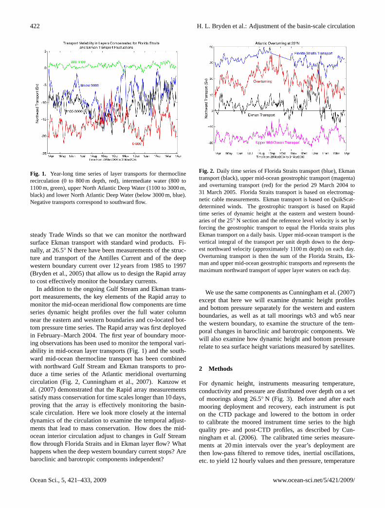
Fig. 1. Year-long time series of layer transports for thermoclinerecirculation (0 to 800 m depth, red), intermediate water (800 to1100 m, green), upper North Atlantic Deep Water (1100 to 3000 m,black) and lower North Atlantic Deep Water (below 3000 m, blue).Negative transports correspond to southward flow.

steady Trade Winds so that we can monitor the northwardsurface Ekman transport with standard wind products. Fi-nally, at 26.5◦ N there have been measurements of the struc-ture and transport of the Antilles Current and of the deepwestern boundary current over 12 years from 1985 to 1997(Bryden et al., 2005) that allow us to design the Rapid arrayto cost effectively monitor the boundary currents.

In addition to the ongoing Gulf Stream and Ekman trans-port measurements, the key elements of the Rapid array tomonitor the mid-ocean meridional flow components are timeseries dynamic height profiles over the full water columnnear the eastern and western boundaries and co-located bot-tom pressure time series. The Rapid array was first deployedin February–March 2004. The first year of boundary moor-ing observations has been used to monitor the temporal vari-ability in mid-ocean layer transports (Fig. 1) and the south-ward mid-ocean thermocline transport has been combinedwith northward Gulf Stream and Ekman transports to pro-duce a time series of the Atlantic meridional overturningcirculation (Fig. 2, Cunningham et al., 2007). Kanzow etal. (2007) demonstrated that the Rapid array measurementssatisfy mass conservation for time scales longer than 10 days,proving that the array is effectively monitoring the basin-scale circulation. Here we look more closely at the internaldynamics of the circulation to examine the temporal adjust-ments that lead to mass conservation. How does the mid-ocean interior circulation adjust to changes in Gulf Streamflow through Florida Straits and in Ekman layer flow? Whathappens when the deep western boundary current stops? Arebaroclinic and barotropic components independent?

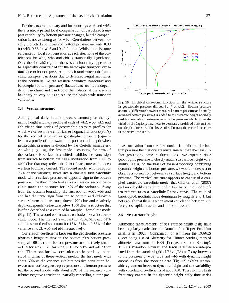
Fig. 2. Daily time series of Florida Straits transport (blue), Ekmantransport (black), upper mid-ocean geostrophic transport (magenta)and overturning transport (red) for the period 29 March 2004 to31 March 2005. Florida Straits transport is based on electromag-netic cable measurements. Ekman transport is based on QuikScat-determined winds. The geostrophic transport is based on Rapidtime series of dynamic height at the eastern and western bound-aries of the 25◦ N section and the reference level velocity is set byforcing the geostrophic transport to equal the Florida straits plusEkman transport on a daily basis. Upper mid-ocean transport is thevertical integral of the transport per unit depth down to the deep-est northward velocity (approximately 1100 m depth) on each day.Overturning transport is then the sum of the Florida Straits, Ek-man and upper mid-ocean geostrophic transports and represents themaximum northward transport of upper layer waters on each day.

We use the same components as Cunningham et al. (2007)except that here we will examine dynamic height profilesand bottom pressure separately for the western and easternboundaries, as well as at tall moorings wb3 and wb5 nearthe western boundary, to examine the structure of the tem-poral changes in baroclinic and barotropic components. Wewill also examine how dynamic height and bottom pressurerelate to sea surface height variations measured by satellites.

2 Methods

For dynamic height, instruments measuring temperature,conductivity and pressure are distributed over depth on a setof moorings along 26.5◦ N (Fig. 3). Before and after eachmooring deployment and recovery, each instrument is puton the CTD package and lowered to the bottom in orderto calibrate the moored instrument time series to the highquality pre- and post-CTD profiles, as described by Cun-ningham et al. (2006). The calibrated time series measure-ments at 20 min intervals over the year’s deployment arethen low-pass filtered to remove tides, inertial oscillations,etc. to yield 12 hourly values and then pressure, temperature

Ocean Sci., 5, 421–433, 2009 www.ocean-sci.net/5/421/2009/

H. L. Bryden et al.: Adjustment of the basin-scale circulation 423

Longitude

Latitude

−80 −70 −60 −50 −40 −30 −20 −1022

24

26

28

30

0

100020003000400050006000

6000

5000

4000

3000

2000

1000

0

1.92

2

333

4444

666888 10101010 121212

141414161616

181818 202020 222222 2424

MA

R1 MA

R3

MA

R2

0

6000

5000

4000

3000

2000

1000

1.8

1.8

1.91.9

22

33

44

6688 1010 1212 1414 1616

18182022

24

Dep

th(m

etre

s)

WB

1

WB

2

WB

3

WB

H2

WB

H1

WB

5

6000

5000

4000

3000

2000

1000

0

2

33

444

666

888

101010121212

14 14 14161616

1818182020

CTD

Current Meter

BPREB

1

EB

H1

EB

H2

EB

H3

EB

H4

EB

H5

3

77o 76.8o 76.6o 76.4o 76.2o 76o 74o 72o 70o

Longitude (degrees West)24o 22o 20o 18o 16o 14o

Longitude (degrees West) Longitude (degrees West)50o 48o 46o 44o 42o

Western Boundary Sub-Array - 2004 Mid-Atlantic Ridge Sub-Array - 2004 Eastern Boundary Sub--Array - 2004

Longitude

Latitude

−80 −70 −60 −50 −40 −30 −20 −1022

24

26

28

30

0

100020003000400050006000

6000

5000

4000

3000

2000

1000

0

1.92

2

333

4444

666888 10101010 121212

141414161616

181818 202020 222222 2424

MA

R1 MA

R3

MA

R2

0

6000

5000

4000

3000

2000

1000

1.8

1.8

1.91.9

22

33

44

6688 1010 1212 1414 1616

18182022

24

Dep

th(m

etre

s)

WB

1

WB

2

WB

3

WB

H2

WB

H1

WB

5

6000

5000

4000

3000

2000

1000

0

2

33

444

666

888

101010121212

14 14 14161616

1818182020

CTD

Current Meter

BPREB

1

EB

H1

EB

H2

EB

H3

EB

H4

EB

H5

3

77o 76.8o 76.6o 76.4o 76.2o 76o 74o 72o 70o

Longitude (degrees West)24o 22o 20o 18o 16o 14o

Longitude (degrees West) Longitude (degrees West)50o 48o 46o 44o 42o

Western Boundary Sub-Array - 2004 Mid-Atlantic Ridge Sub-Array - 2004 Eastern Boundary Sub--Array - 2004

Fig. 3. Rapid array along 26.5◦ N during 2004–2005:(a) location in latitude and longitude of each mooring;(b) location of instruments versusdepth and longitude along 26.5◦ N. Only instruments that returned year-long time series are shown. Principal components are 15 bottompressure records and 12 dynamic height moorings concentrated near the western and eastern boundaries.

and salinity are used to calculate specific volume anomalytime series that are then integrated vertically to produce dy-namic height profiles at each mooring site. Cunningham etal. (2007) described how the dynamic height profile fromthe surface to 4820 dbar at the western boundary is createdby joining measurements on wb2, wbh1 and wbh2 and howthe dynamic height profile at the eastern boundary from thesurface to 5200 dbar is created by joining measurements onmoorings eb1, ebh2, ebh3, ebh4 and ebh5 crawling up thecontinental slope. We will refer to these western and easternboundary profiles as dynamic height at wb2 and ebh. Sim-ilarly, dynamic height profiles are created for the tall wb3and wb5 moorings 50 km and 500 km east from the westernboundary. For each site (wb2, wb3, wb5 and ebh), we thencreate a temporal mean dynamic height profile over the pe-riod March 2004 to April 2005. The difference between themean eastern and western dynamic height profiles, when di-vided by the Coriolis parameter and vertically integrated, isequal to the mean geostrophic mid-ocean meridional trans-port. This geostrophic mid-ocean transport must balance themean Gulf Stream plus Ekman transport and this constrainteffectively sets the mean reference level velocity (and meanbottom pressure difference), as described by Cunningham etal. (2007). Here, we examine the 12 h anomalies in dynamicheight with respect to the mean profiles at each site.

For bottom pressure, the 2004–2005 Rapid array included15 bottom pressure gauges: from west to east, they were atthe following moorings (Fig. 3):

wb1, wb2, wbh1, wbh2, wb3, wb5, mar2, mar1, mar3, eb1,ebh1, ebh2, ebh3, ebh4, and ebh5.

wb1 and ebh5 are very shallow; wbh2 is not consistent withsurrounding records on wb2, wbh1 and wb3; mar1 suffers

from mooring motion as it floated slightly above the bottom;and ebh1 appears to have a jump in mid record. Thus, weconcentrate here on 10 deep bottom pressure records acrossthe width of the North Atlantic at about 26.5◦ N:

wb2, wbh1, wb3, wb5, mar2, mar3, eb1, ebh2, ebh3, andebh4.

Four are near the western boundary, two on the Mid AtlanticRidge, and four near the eastern boundary, so there is a rel-atively even distribution across the Atlantic but with fournear the eastern and four near the western boundaries. Eachrecord consists of 20 min time series of pressure and tem-perature. Each record is low-pass filtered to remove semi-diurnal and diurnal tides, and an exponential trend is re-moved to account for drift in each pressure sensor (Fig. 4;Kanzow, 2006). In addition, each record has been analysedto estimateMf andMm 14-day and 28-day tidal constituentsand these components have been subtracted out of the pres-sure records. Finally, since the exact depth of each pressuregauge is not known, the record-length average pressure is re-moved for each pressure gauge and we examine here the 12 hanomaly in bottom pressure for each site.

Gulf Stream transport is obtained on a daily basis fromthe Florida Straits cable time series (www.aoml.noaa.gov/phod/floridacurrent). Ekman transport is estimated on a dailybasis by dividing QuikScat zonal wind stress values (http://winds.jpl.nasa.gov/missions/quikscat/index.cfm) by the sur-face density and by the Coriolis parameterf and integratingzonally across the basin at 26◦ N.

To examine relations between dynamic height, bottompressure, sea surface height, Gulf Stream and Ekman trans-ports, we calculate correlation coefficients versus time lag.In general maximum correlation occurs with zero time lag,

www.ocean-sci.net/5/421/2009/ Ocean Sci., 5, 421–433, 2009

www.aoml.noaa.gov/phod/floridacurrent

www.aoml.noaa.gov/phod/floridacurrent

http://winds.jpl.nasa.gov/missions/quikscat/index.cfm

http://winds.jpl.nasa.gov/missions/quikscat/index.cfm


Fig. 4. Bottom pressure record at mooring wb2. 20 min valuesexhibit strong tidal oscillations and a clear exponential drift withtime is also apparent due to sensor creep (upper curves offset by1 dbar). After tidal filtering and removing the exponential drift, thelow-passed 12 hourly time series of bottom pressure (lower curve,mean removed) reveals an rms amplitude of 0.022 dbar.

unless reported otherwise. Cunningham et al. (2007) haveestimated the integral time scales for temporal variability inthe time series used here to be 24 days. For the 366 daytime series, there are then 15 independent time periods, or13 degrees of freedom, from which we determine that cor-relations greater than 0.514 are significantly different fromzero at a 95% confidence level. We therefore concentratediscussion in the text on correlations greater than 0.51.

3 Analysis

3.1 Baroclinic variability

We first assess the contributions to variability resulting fromtemperature and salinity anomalies at the western and easternboundaries; we will call this baroclinic variability. Dynamicheight anomaly profiles divided by Coriolis parameter yieldgeostrophic velocity anomaly profiles that can be integratedvertically to yield local transport variability following themethodology described by Longworth (2007). First we inte-grate the dynamic height anomalies from bottom to surface toestimate the total west (wb2) and east (ebh) baroclinic trans-port variability (Fig. 5). The variance in the west is a factorof five larger than that at the east with standard deviations inwestern and eastern baroclinic transport of 7.9 Sv and 3.3 Svrespectively. We can also do the vertical integration over lay-ers and we choose the same depth intervals used by Cun-ningham et al. (2007) to estimate the transport variability inthe thermocline recirculation (0 to 800 m depth), intermedi-ate water (800 to 1100 m), upper North Atlantic Deep Water

Fig. 5. Baroclinic transport variability near the western and easternboundaries. Dynamic height anomaly profiles are vertically inte-grated on a daily basis and divided by the Coriolis parameter toyield baroclinic transport variability in Sverdrups. Dynamic heightat the west is made up from temperature-salinity-pressure time se-ries on moorings wb2, wbh1 and wbh2 and at the east from timeseries on moorings eb1, ebh1, ebh2, ebh3 ebh4, as described byCunningham et al. (2007).

(UNADW, 1100 to 3000 m) and lower North Atlantic DeepWater (LNADW, below 3000 m) for the western (wb2) andeastern (ebh) sites (Table 1). The transport variability in thethermocline recirculation (0 to 800 m depth) is only slightlylarger in the west than in the east; but variability in deepwater transports is much greater in the west as there is verylittle deep transport variability in the east at ebh. Thus, asfound also by Longworth (2007) in an analysis of historicalhydrographic stations, baroclinic variability near the westernboundary is much larger than that at the eastern boundary.

3.2 Bottom pressure

For bottom pressure, the first notable feature of the 10 bot-tom pressure records is that the pressure goes up and downin unison for all 10 pressure gauges (Fig. 6a). The stan-dard deviation (equal to the root mean square value or rms)of the 12 hourly zonal average (over 10 records) pressure is0.0150 dbar. All across the ocean at 26.5◦ N, bottom pressurerises and falls on about a 5 to 10 day time scale with an rmsamplitude equivalent to an rms rise and fall in sea level ofabout 1.5 cm. The entire Atlantic Ocean at 26◦ N appears tobe filling and draining (see Appendix A for a brief analysisof the origins of the zonally averaged pressure fluctuations).To remove this signal so as to avoid contaminating local bot-tom pressure fluctuations with the strong fluctuations in zon-ally averaged bottom pressure, we subtract the zonal averagepressure (Fig. 6b, a straight average of the 10 bottom pres-sure records) from each individual record at each 12 h inter-val. The resulting rms pressure signal is reduced from about



Fig. 6. Bottom pressure time series:(a) at 10 sites across the At-lantic at 26.5◦ N (each offset by 0.08 dbar) and(b) the zonal aver-age bottom pressure on each day (offset by−0.05 dbar). Note thatbottom pressure appears to rise and fall in phase at all 10 sites.

0.019 dbar to about 0.012 dbar, a 60% reduction in variance(Table 2). To put the values in context, a 0.02 dbar bottompressure signal, if it is depth independent over 5000 m depthand in geostrophic balance and unmatched by the same signalon the other side of the basin, would represent a geostrophictransport signal of 15 Sv. Clearly, however, to first order thehigh frequency bottom pressure fluctuations on the west andon the east have similar amplitude so their difference whichis proportional to a barotropic transport is much smallerthan their individual amplitudes. Again the variance in bot-tom pressure is larger at the west than at the east, but onlyslightly larger (excluding the wb5 record that looks some-what anomalous).

3.3 Baroclinic-barotropic compensation

Baroclinic transport anomalies arise due to changes in tem-perature and salinity. Right at the western boundary, they areperhaps due to Rossby waves or eddies propagating west-ward and hitting the boundary or perhaps due to Kelvinwaves propagating southward along the continental slope. Atthe eastern boundary the anomalies may be due to changes inthe upwelling regime or to Kelvin waves propagating north-ward along the continental slope. In the calculations byCunningham et al. (2007) that assumed mass compensation,a baroclinic transport anomaly is compensated by a depth-independent or barotropic adjustment in the basin-scale flow.We might hypothesise a local barotropic adjustment to abaroclinic transport anomaly whereby the bottom pressurechanges each day at the base of the mooring so that the ver-tical integral of the bottom pressure anomaly (bottom pres-sure anomaly times 4800 m depth) exactly cancels the baro-

Table 1. Baroclinic Transport Standard Deviation (Sv). Transportsare vertically integrated dynamic height anomaly divided byf .

East West

Overall 3.32 7.89

0–800 m 2.43 2.97800–1100 m 0.49 0.871100–3000 m 0.70 4.22Below 3000 m 0.08 0.77

Table 2. Bottom Pressure Variability. Each pressure record hashad an exponential drift removed, each has been low-pass filteredto remove high frequency tidal and intertial oscillations, and eachhas been fitted to remove fortnightlyMf and monthlyMm tidalcomponents. The resulting bottom pressure variations exhibit stan-dard deviations ranging from 0.016 to 0.026 dbar. All records ex-hibit synchronous rise and fall of pressure on a 5 to 10 day timescale. Thus we estimate a zonally averaged bottom pressure overthe 10 records (Fig. 4b) and remove it from each bottom pressurerecord. The zonally averaged bottom pressure has a standard devia-tion of 0.0150 dbar. After removing the zonally avearged pressure,the resulting bottom pressure records exhibit standard deviationsranging from 0.009 to 0.022 dbar, a 60% reduction in variance.

Mooring Individual-Averagestd dev std dev(dbar) (dbar)

wb2 0.0218 0.0118wbh1 0.0226 0.0131wb3 0.0210 0.0109wb5 0.0261 0.0215mar2 0.0173 0.0105mar3 0.0168 0.0100eb1 0.0189 0.0146ebh2 0.0157 0.0094ebh3 0.0165 0.0102ebh4 0.0165 0.0095

clinic transport anomaly observed on the mooring that day.The resulting pressure profile (dynamic height profile rel-ative to the bottom + predicted bottom pressure) then haszero vertical integral, and the total transport anomaly is zero.Thus, locally we can predict a compensating bottom pres-sure anomaly for each day so that the overall local transportanomaly (barotropic + baroclinic transport) is zero.

Remarkably, at the western boundary at wb2 this pre-dicted bottom pressure anomaly is strongly correlated withthe observed bottom pressure time series after subtracting outthe zonally uniform signal (Fig. 7): observed and predictedbottom pressures at wb2 have similar amplitude, no appar-ent phase shift and a significant correlation of 0.62. Thus,the bottom pressure at the western boundary appears to be



Fig. 7. Bottom pressure at wb2. The bottom pressure anomaly(blue) is defined to be the bottom pressure measured at wb2 mi-nus the zonal average bottom pressure shown in Fig. 6b. Predictedbottom pressure (red) is that required to compensate for local baro-clinic transport variability shown in Fig. 5. The difference betweenbottom pressure anomaly and predicted bottom pressure at wb2 isshown in black. The blue and red curves have been offset from theblack curve by adding 0.06 dbar to them.

responding to local changes in baroclinic transport due tofluctuations in temperature and salinity and compensating forvariations in baroclinic transport.

To describe this baroclinic transport compensation mech-anism with an example, we examine the event in earlyNovember 2004 that is the largest event in both baroclinictransport anomaly and bottom pressure anomaly. In earlyNovember, deep temperatures at the western boundary (wb2)warmed substantially with isotherms deepening by about700 m (Fig. 8). Such anomalous warming leads to positivedynamic height anomaly as indicated in Fig. 9 (blue) leadingto a mid-ocean southward transport anomaly if the easternboundary dynamic height anomaly remains constant. For thisevent the transport anomaly is more than 30 Sv (Fig. 5). Thepredicted bottom pressure anomaly to compensate the trans-port anomaly is a negative offset whose vertical integral bal-ances the vertically integrated dynamic height. Remarkably,the observed bottom pressure anomaly at wb2 is almost ex-actly equal to the predicted compensation pressure as shownin Fig. 7. The resulting dynamic pressure anomaly profile,bottom pressure + dynamic height (Fig. 9, green) is then sub-tracted from the mean transport per unit depth profile (Fig. 9,black) to produce the mid-ocean transport per unit depth pro-file (Fig. 9, red) that shows that the southward transport oflower North Atlantic Deep water (LNADW) below 3000 meffectively stopped during this event. From associated directmeasurements during this event, Johns et al. (2008) also ob-served the stoppage in the southward flow of LNADW.

Fig. 8. Contoured time series of temperature profiles measuredon wb2 at the western boundary. Note the steep descent of deepisotherms in early November 2004 that marks the shutdown in thesouthward flow of lower North Atlantic Deep water.

Fig. 9. Vertical profiles of transport per unit depth during theNovember 2004 event at wb2. The mean mid-ocean transport perunit depth profile (black line) is derived from the difference betweentime-averaged dynamic height profile2 at ebh and wb2. The dy-namic height anomaly profile for the November event at wb2 (blueline) reflects the presence of warmer deep waters at the westernboundary as seen in Fig. 8. The dynamic height profile + the ob-served bottom pressure anomaly at wb2 (green line) represents thetotal anomaly profile for the November event at the western bound-ary. The final mid-ocean transport per unit depth profile for theNovember event (red line) is the difference between the mean pro-file and the anomaly profile and assumes zero anomaly at the easternboundary. Note the shutdown in the southward flow of lower NorthAtlantic Deep water below 3000 m depth with an actual reversal tonorthward flow below 3500 m depth.



For the eastern boundary and for moorings wb3 and wb5,there is also a partial local compensation of baroclinic trans-port variability by bottom pressure changes, but the compen-sation is not as strong as for wb2. Correlations between lo-cally predicted and measured bottom pressure are only 0.09for wb3, 0.38 for wb5 and 0.42 for ebh. Whilst there is someevidence for local compensation at each site, none of the cor-relations for wb3, wb5 and ebh is statistically significant.Only the site wb2 right at the western boundary appears tobe especially constrained for the barotropic transport varia-tions due to bottom pressure to match (and cancel) the baro-clinic transport variations due to dynamic height anomaliesat the boundary. At the western boundary, baroclinic andbarotropic (bottom pressure) fluctuations are not indepen-dent; baroclinic and barotropic fluctuations at the westernboundary co-vary so as to reduce the basin-scale transportvariations.

3.4 Vertical structure

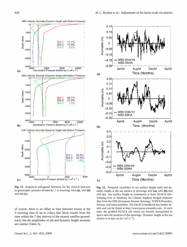
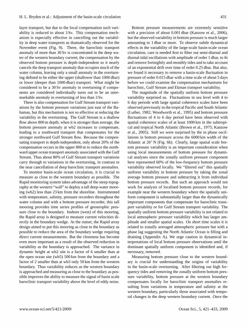
Adding local daily bottom pressure anomaly to the dy-namic height anomaly profile at each of wb2, wb3, wb5 andebh yields time series of geostrophic pressure profiles forwhich we can estimate empirical orthogonal functions (eof’s)for the vertical structure in geostrophic pressure (equiva-lent to a profile of northward transport per unit depth whengeostrophic pressure is divided by the Coriolis parameter).At wb2 (Fig. 10), the first mode accounting for 56% ofthe variance is surface intensified, exhibits the same signfrom surface to bottom but has a modulation from 1000 to4000 dbar that may reflect the 2-lobed structure of the deepwestern boundary current. The second mode, accounting for23% of the variance, looks like a classical first baroclinicmode with a surface pressure of opposite sign to the bottompressure. The third mode looks like a classical second baro-clinic mode and accounts for 14% of the variance. Awayfrom the western boundary, the first eof for wb3, wb5 andebh has the same sign from top to bottom and exhibits asurface intensified structure above 1000 dbar and relativelydepth-independent structure below 1000 dbar, a structure thatis often described as a coupled barotropic – baroclinic mode(Fig. 11). The second eof in each case looks like a first baro-clinic mode. The first eof’s account for 71%, 61% and 61%and the second eof’s account for 18%, 31% and 37% of thevariance at wb3, wb5 and ebh, respectively.

Correlation coefficients between the geostrophic pressure(dynamic height relative to the bottom plus bottom pres-sure) at 100 dbar and bottom pressure are relatively small:−0.14 for wb2, 0.20 for wb3, 0.16 for wb5 and−0.23 forebh. The reason for low correlation can be partially under-stood in terms of these vertical modes: the first mode withabout 60% of the variance exhibits positive correlation be-tween near-surface geostrophic pressure and bottom pressurebut the second mode with about 25% of the variance con-tributes negative correlation, partially cancelling out the pos-

Fig. 10. Empirical orthogonal functions for the vertical structurein geostrophic pressure divided byf at wb2. Bottom pressureanomaly (difference between measured bottom pressure and zonallyaveraged bottom pressure) is added to the dynamic height anomalyprofile at each day to estimate geostrophic pressure which is then di-vided by the Coriolis parameter to generate a profile of transport perunit depth in m2 s−2. The first 3 eof’s illustrate the vertical structurein the daily time series.

itive correlation from the first mode. In addition, the bot-tom pressure fluctuations are much smaller than the near sur-face geostrophic pressure fluctuations. We expect surfacegeostrophic pressure to closely match sea surface height vari-ability. Thus, on the basis of these 4 moorings combiningdynamic height and bottom pressure, we would not expect toobserve a correlation between sea surface height and bottompressure. The vertical structure appears to consist of a cou-pled barotropic-baroclinic mode, that Chelton et al. (2007)call an eddy-like structure, and a first baroclinic mode, of-ten referred to as a baroclinic Rossby wave. The coupledbarotropic-baroclinic mode dominates by roughly 2 to 1, butnot enough that there is a consistent correlation between sur-face geostrophic pressure and bottom pressure.

3.5 Sea surface height

Altimetric measurements of sea surface height (ssh) havebeen regularly made since the launch of the Topex-Poseidonsatellite in 1992. Comparison of ssh from the DUACS(Developing Use of Altimetry for Climate Studies) mergedaltimeter data from the ERS (European Remote Sensing),TOPEX/Poseidon, Envisat, and Jason satellites are interpo-lated from the standard grid (1/3◦

×1/3◦) at 7-day intervalsto the positions of wb2, wb3 and wb5 with dynamic heightanomalies from the mooring data (Fig. 12) exhibit reason-able agreement between dynamic height and ssh variabilitywith correlation coefficients of about 0.8. There is more highfrequency content in the dynamic height daily time series



(a)

(b)

(c)

Fig. 11. Empirical orthogonal functions for the vertical structurein geostrophic pressure divided byf at moorings wb3(a), wb5 (b)and ebh(c).

of course; there is an offset in time between events at the3 mooring sites of up to 2 days that likely results from thetime within the 7 day interval of the nearest satellite ground-track; but the amplitudes of ssh and dynamic height anomalyare similar (Table 3).

(a)

(b)

(c)

Fig. 12. Temporal variability in sea surface height (ssh) and dy-namic height at the sea surface at moorings wb2(a), wb3 (b) andwb5 (c). Sea surface height in centimetres is from DUACS (De-veloping Use of Altimetry for Climate Studies) merged altimeterdata from the ERS (European Remote Sensing), TOPEX/Poseidon,Envisat, and Jason satellites. The DUACS handbook has further de-tails and can be found athttp://www.jason.oceanobs.com. At eachtime, the gridded DUACS ssh values are linearly interpolated inspace onto the position of the moorings. Dynamic height at the seasurface is in dyn cm (0.1 m2 s−2).


http://www.jason.oceanobs.com


Table 3. Standard Deviation of Sea Surface Height (ssh) and Dy-namic Height. The ssh values are for the time period 29 March2004 to 31 March 2005 to match the time period of the dynamicheight variations. The ssh values in parentheses are for the 13 yeartime period 1992–2005. 100 dbar is typically the shallowest instru-ment depth in the Rapid array so dynamic height at the surface is anextrapolation of the dynamic height anomaly from 100 dbar to thesurface.

ssh dynamic height dynamic height(100 dbar) (0 dbar)

Site (cm) (dynamic cm) (dynamic cm)

wb2 4.83 (5.50) 3.46 4.66wb3 6.22 (6.78) 5.40 7.24wb5 7.66 (9.66) 8.64 10.57

It is notable that both ssh and dynamic height show a de-crease in variance toward the boundary (Fig. 13). On itsown, the striking decrease in the variance in ssh as land isapproached might have reasonably been considered to be theresult of boundary effects in the satellite altimetric measure-ments. However, the dynamic height time series also showa striking decrease in variance with the standard deviation in100 dbar dynamic height decreasing from 8.6 dynamic cen-timetres at wb5, 500 km from the boundary, to 5.4 at wb350 km from the shore, to 3.5 at wb2 23 km from Abaco. Re-markably, the western boundary appears to exert a strongconstraint on the size of variability in ssh and dynamic heightrelative to offshore variability. Kanzow et al. (2009) providedynamical arguments for how eddies interact with the west-ern boundary leading to this sharp decrease in eddy ampli-tude close to the boundary.

3.6 Gulf Stream and Ekman transport compensation

It is of interest to know how the fluctuations in Gulf Streamtransport are balanced by the mid-ocean flow. Cunninghamet al. (2007) already reported that the Gulf Stream, Ekmanand mid-ocean thermocline components of the overturningare not significantly correlated, so we concentrate here oncompensation by bottom pressure fluctuations. We first re-moved the predicted bottom pressure based on baroclinictransport variations from the observed bottom pressure atwb2 in order to examine how this reduced pressure anomalyrelates to the Gulf Stream transport through Florida Straits.We multiply the reduced bottom pressure at wb2 by 4000 mdepth and divide by the Coriolis parameter to derive a timeseries of geostrophic mid-ocean transport due to fluctuationsat wb2. The baroclinic transport anomaly has already beencompensated by the predicted part of the bottom pressurethat we removed. Thus, the reduced pressure anomaly rep-resents the residual geostrophic transport that is effectivelybarotropic. The resulting geostrophic mid-ocean transport

Fig. 13. Standard deviation in sea surface height variabil-ity (cm) versus longitude at 26.5◦ N. The continuous curve isfrom DUACS (Developing Use of Altimetry for Climate Studies)merged altimeter data from the ERS (European Remote Sensing),TOPEX/Poseidon, Envisat, and Jason satellites. The standard de-viation in dynamic height at moorings wb2, wb3, wb5 and ebh areindicated by crosses at the appropriate longitudes. The horizontalscale is expanded west of 70◦ W to show the sharp drop in ssh (anddynamic height) variability as the western boundary is approached.

time series is correlated to the fluctuations in Gulf Streamtransport through Florida Straits: for daily values the corre-lation is 0.51 and for 10-day low-passed values the correla-tion is 0.61. The sign of the correlation is notable: higherGulf Stream transport is correlated with higher bottom pres-sure at the western boundary at wb2 which indicates south-ward barotropic geostrophic transport in the interior basin at26◦ N. The correlation falls rapidly, at wb3 50 km east of theBahamas the correlation has dropped to 0.34 and by wb5 thecorrelation has effectively vanished. The geostrophic trans-port associated with the bottom pressure anomaly at the west-ern boundary is noisy but a scatter plot (Fig. 14) shows a clearrelationship between reduced bottom pressure anomalies andGulf Stream transport fluctuations. Arguably, the amplitudeof the reduced bottom pressure is even correct, remarkable inthat we just chose 4000 m as the depth over which to applythe barotropic transport; choosing 4230 m for the depth scalewould have led to the barotropic transport variations havingthe same rms amplitude as the Gulf Stream transport varia-tions.

We were unable to increase the correlation between GulfStream transport and bottom pressure fluctuations, for exam-ple by using the difference between wb2 and wb3 or betweenwb2 and eb1. Thus, fluctuations in the Gulf Stream transportthrough Florida Straits appear to be balanced by a compen-sating change in bottom pressure right at the western bound-ary of the mid-ocean section. The compensation appears tobe instantaneous though we admit that the remnant bottom



Fig. 14. Scatter plot of bottom pressure at wb2 and Gulf Streamtransport anomaly (Sv). The bottom pressure is the difference be-tween bottom pressure anomaly at wb2 and the predicted bottompressure required to compensate for baroclinic transport variationsat wb2 (as described in Fig. 7). This bottom pressure is then multi-plied by a scale depth of 4000 m and divided byf to convert it intoa western boundary transport anomaly in Sv. Both bottom pressureand Gulf Stream transport time series have been low-passed filteredwith a cut-off at 10-day period. The correlation coefficient for thetwo time series is 0.62.

pressure time series remains quite noisy after removing thetides, an exponential drift, a fluctuating basin-scale averagebottom pressure and a bottom pressure component that com-pensates for baroclinic transport variations at wb2.

For fluctuations in Ekman transport, we first examinedcorrelations between Ekman transport and bottom pressurerecords at wb2, wbh1, wb3, wb5, wb2, wbh1, wb3, wb5,mar3, mar2, eb1, ebh2, ebh3, ebh4 and found highest cor-relations at wbh1 (0.41) and eb1 (−0.44). Taking the dif-ference wbh1–eb1 led to an even higher correlation of 0.47and for 10-day low-passed series the correlation increased to0.57. An eof analysis for the zonal structure in bottom pres-sure yields a first mode with high pressure near the westernboundary and low pressure in the eastern boundary account-ing for 46% of the variance. The first mode time series is alsocorrelated with Ekman transport variability at 0.36. Thus,variations in Ekman transport appear to be compensated bya bottom pressure difference that spans the ocean basin fromthe western boundary at wbh1 to the eastern boundary at eb1.We rationalise the small correlation (0.11) between Ekmantransport and wb2 bottom pressure as being due to the sig-nal at wb2 being masked by the larger baroclinic and GulfStream compensations at wb2. More troubling is that the bot-tom pressure difference fluctuations (when turned into trans-port by multiplying by 4000 m depth and dividing byf ) ap-pear to be a factor of 3 larger than the variations in Ekman

transport. Thus, although there is good correlation betweenbasin-scale bottom pressure difference and Ekman transport,the magnitude of the barotropic flow derived from the bottompressure difference is much larger than the Ekman transportand as a result we feel we do not yet understand how the vari-ations in Ekman transport are compensated in the basin-scalecirculation.

4 Discussion

The variability in the meridional overturning circulation at26◦ N reported by Cunningham et al. (2007) is smaller thananticipated. Based on satellite altimetric estimates of sea sur-face height variability associated with eddies, Wunsch (2008)has recently argued that the rms variability in overturningshould be 16 Sv. In sharp contrast, Cunningham et al. (2007)estimated variability in the upper mid-ocean transport of only3.3 Sv. On the basis of the analysis here, the smallness ofthe observed variability in the overturning at 26◦ N has twocauses: first, eddy variability reduces sharply as the westernboundary is approached; and secondly, there is strong com-pensation between components of the overturning so that theoverall variability in overturning is much smaller than thevariability in individual components.

Eddy variability in both upper ocean dynamic height andsea surface height (ssh) decreases markedly westward along26◦ N as the western boundary of the Bahamas is approached(Fig. 11). When we first plotted ssh variability from satellitealtimeters versus longitude, colleagues said that the reduc-tion in variability near the western boundary was due to landeffects in the satellite measurements. But the dynamic heighttime series from the moorings show agreement in amplitudeand timing with the satellite ssh time series and the dynamicheight variance also decreases toward the boundary. Thus theevidence is compelling that variability in sea surface heightindeed decreases toward the western boundary. Our initialqualitative argument was that eddies generate most of theupper ocean variability in ssh and that the centre of a cir-cular eddy could not make it to the coastline because theflow of the eddy toward the boundary would quickly moveaway along the boundary so the eddy would decay as it ap-proached the boundary. Kanzow et al. (2009) have now putsuch a qualitative argument into a dynamical framework toshow how eddies or waves dissipate as they approach thewestern boundary.

In terms of compensating components, Kanzow etal. (2007) showed a remarkable compensation between whatthey called the internal and external modes of variability.Here we find that the baroclinic transport (internal mode)variability at the western boundary with an rms value of7.9 Sv (Table 1) is compensated locally and instantaneouslyby variability in bottom pressure (external mode) that effec-tively cancels the depth-integrated baroclinic transport vari-ability (Fig. 7). There is still variability in upper (or lower)



layer transport, but due to the local compensation such vari-ability is reduced to about 3 Sv. This compensation mech-anism is especially effective in cancelling out the variabil-ity in deep water transports as dramatically observed for theNovember event (Fig. 9). There, the baroclinic transportanomaly of more than 30 Sv is concentrated in the deep wa-ter of the western boundary current; the compensation by theobserved bottom pressure is depth-independent so it nearlycancels the deep transport anomaly that occupies much of thewater column, leaving only a small anomaly in the overturn-ing defined to be either the upper (shallower than 1000 dbar)or lower (deeper than 1000 dbar) transport. What might beconsidered to be a 30 Sv anomaly in overturning if compo-nents are considered individually turns out to be an unre-markable anomaly in overturning of less than 3 Sv.

There is also compensation for Gulf Stream transport vari-ations by the bottom pressure variations just east of the Ba-hamas, but this mechanism is not so effective at reducing thevariability in the overturning. The Gulf Stream is a shallowflow above 800 m depth; when it is stronger than average, thebottom pressure anomaly at wb2 increases to compensate,leading to a southward transport that compensates for thestronger northward Gulf Stream flow. Because the compen-sating transport is depth-independent, only about 20% of thecompensation occurs in the upper 800 m to reduce the north-ward upper ocean transport anomaly associated with the GulfStream. Thus about 80% of Gulf Stream transport variationscarry through to variations in the overturning, in contrast tothe near cancellation of deep baroclinic transport anomalies.

To monitor basin-scale ocean circulation, it is crucial tomeasure as close to the western boundary as possible. TheRapid monitoring system takes advantage of the steep topog-raphy at the western “wall” to deploy a tall deep-water moor-ing (wb2) less than 23 km from the shoreline. Instrumentedwith temperature, salinity, pressure recorders throughout thewater column and with a bottom pressure recorder, this tallmooring provides time series profiles of geostrophic pres-sure close to the boundary. Inshore (west) of this mooring,the Rapid array is designed to measure current velocities di-rectly in the boundary wedge. At the outset, the Rapid arraydesign aimed to put this mooring as close to the boundary aspossible to reduce the area of the boundary wedge requiringdirect current measurements. But the closeness has becomeeven more important as a result of the observed reduction invariability as the boundary is approached. The variance indynamic height at wb2 site is a factor of 6 smaller than atthe open ocean site (wb5) 500 km from the boundary and afactor of 2 smaller than at wb3 only 50 km from the westernboundary. Thus variability reduces as the western boundaryis approached and measuring as close to the boundary as pos-sible improves the ability to measure the signal of basin scalebaroclinic transport variability above the level of eddy noise.

Bottom pressure measurements are extremely sensitivewith a precision of about 0.001 dbar (Kanzow et al., 2006),but the observed variability in bottom pressure is much largeramounting to 1 dbar or more. To observe subtle dynamicaleffects in the variability of the large-scale basin-scale oceancirculation, care is needed first to filter out semi-diurnal anddiurnal tidal oscillations with amplitude of order 1 dbar, to fitand remove fortnightly and monthly tides and to take accountof an exponential drift over time of order 0.25 dbar. But also,we found it necessary to remove a basin-scale fluctuation inpressure of order 0.015 dbar with a time scale of about 5 daysbefore we could examine the compensation mechanisms forbaroclinic, Gulf Stream and Ekman transport variability.

The magnitude of the spatially uniform bottom pressurevariability surprised us. Fluctuations in sea level with 4 to6 day periods with large spatial coherence scales have beenobserved previously in the tropical Pacific and South Atlantic(Luther, 1982; Woodworth et al., 1995) and bottom pressurefluctuations of 4 to 6 day period have been observed withspatial coherence scales of at least 1000 km in the subtropi-cal and tropical North Atlantic (Brown et al., 1975; Kanzowet al., 2005). Still we were surprised by the in phase oscil-lations in bottom pressure across the 6000 km width of theAtlantic at 26◦ N (Fig. 6b). Clearly, large spatial scale bot-tom pressure variability is an important consideration whenusing local measurements of bottom pressure for dynami-cal analyses since the zonally uniform pressure componenthere represented 60% of the low-frequency bottom pressurevariability observed locally. We “filtered out” this spatiallyuniform variability in bottom pressure by taking the zonalaverage bottom pressure and subtracting it from individualbottom pressure records. But such an approach would notwork for analysis of localised bottom pressure records, forexample near the western boundary where the spatially uni-form component is substantially larger than the dynamicallyimportant components that compensate for baroclinic trans-port variability or for Gulf Stream transport variability. Thespatially uniform bottom pressure variability is not related tolocal atmospheric pressure variability which has larger am-plitude and smaller spatial scales. On short time scales it isrelated to zonally averaged atmospheric pressure but with aphase lag suggesting the North Atlantic Ocean is filling anddraining (Appendix A). We urge caution in dynamical in-terpretations of local bottom pressure observations until thedominant spatially uniform component is identified and, ifnecessary, removed.

Measuring bottom pressure close to the western bound-ary is crucial for understanding the origins of variabilityin the basin-scale overturning. After filtering out high fre-quency tides and removing the zonally uniform bottom pres-sure variability, bottom pressure at the western boundarycompensates locally for baroclinic transport anomalies re-sulting from variations in temperature and salinity at thewestern boundary, particularly those associated with tempo-ral changes in the deep western boundary current. Once the



baroclinic transport compensating pressure is removed fromthe bottom pressure time series, the residual variability inbottom pressure close to the boundary compensates for GulfStream transport anomalies. This Gulf Stream compensatingbottom pressure appears to decay quickly eastward from theboundary as it has mostly disappeared at wb3 50 km east ofwb2. There may also be a component that compensates forEkman transport variability but the small errors in estimatingthe residual bottom pressure fluctuations by subtracting outthe tidal, zonally uniform, baroclinic and Gulf Stream com-ponents compromises our ability to observe this componentat the western boundary site wb2. Thus to understand themechanisms that balance variations in Gulf Stream transportand deep western boundary current structure, it is essentialto measure bottom pressure right at the western boundary.

It is rare to have full-depth moorings measuring temper-ature and salinity time series throughout the water columnwith associated bottom pressure measurements so that sealevel, atmospheric pressure, geostrophic pressure throughoutthe water column and bottom pressure can be intercomparedand combined to quantify the vertical structure of ocean vari-ability. The Rapid array had 4 tall moorings during 2004–2005: wb2, wb3 and wb5 near the western boundary and ebhnear the eastern boundary. For these moorings we find no sta-tistically significant correlation between bottom pressure andsea surface height (defined to be dynamic height referencedto the bottom plus bottom pressure). Empirical orthogonalmodes reveal no simple projection onto a consistent verti-cal modal structure. Only at the westernmost mooring, wb2,is there a significant anti-correlation between vertically inte-grated dynamic height and bottom pressure fluctuations indi-cating mass compensation between baroclinic and barotropicfluctuations and suggesting a first baroclinic mode structurewith no net vertically integrated flow.

That fluctuations in Gulf Stream and deep western bound-ary current mass transport are instantaneously compensatedby bottom pressure adjustments at the western boundarydemonstrates how tight the overall mass conservation con-straint is for an ocean basin like the North Atlantic that isnearly closed at its northern boundary. Gulf Stream transportfluctuations, rms of 3.3 Sv, or deep western boundary trans-port fluctuations, rms of 4.2 Sv, cannot be compensated byequal inflow or outflow through the shallow Bering Straits.Thus, such transport fluctuations quickly lead to changes insea level height and hence in bottom pressure that can prop-agate at deep water wave speeds of

√gH, or 200 m s−1 for

ocean water depth of 4000 m, to adjust the circulation tobalance the initial transport anomaly. Here we find that theGulf Stream and deep western boundary current fluctuationsare compensated by bottom pressure at the western bound-ary, while Ekman transport fluctuations appear to have a sig-nature in bottom pressure at both the eastern and westernboundaries.

Appendix A

After low-pass filtering the individual bottom pressurerecords to remove high frequency tides, there was a sur-prisingly large pressure variation common to all individualrecords that had a standard deviation of 0.0182 dbar repre-senting about 75% of the low frequency variance in bottompressure. One component of this spatially uniform bottompressure variability is clearly related to the fortnightly andmonthly tidal forcing so we removed these components byfitting and subtractingMf and Mm signals from individ-ual bottom pressure records. TheseMf and Mm compo-nents have a standard deviation of 0.0106 dbar and the rmseast-west bottom pressure difference for these low frequencytidal fluctuations is 0.0048 dbar, suggesting a north-southgeostrophic transport at these tidal frequencies of 3 Sv.

After removing the low frequency tidal components, thezonally averaged bottom pressure had a standard deviationof 0.0150 dbar (Table 2). Much of the variability occursat periods less than 10 days so we examined the relationbetween 10-day high-passed zonally avearged bottom pres-sure, zonally averaged atmospheric pressure and barotropicgeostrophic transport (proportional to east minus west bot-tom pressure difference). For the 4–5 day period, variationsin zonally averaged bottom pressure are coherent with zon-ally averaged atmospheric pressure at 26◦ N (from NCEP)but there is a 30◦ phase difference such that bottom pres-sure peaks 30◦ before atmospheric pressure. There appearsalso to be a phase lag where southward geostrophic trans-port (ebh3–wb2) lags maximum bottom pressure by about30◦. If we combine atmospheric pressure and bottom pres-sure to estimate a sea level time series (sea level = bottompressure – atmospheric pressure), then sea level peaks 30◦

before bottom pressure and southward geostrophic transportoccurs when sea level is falling rapidly, slightly after maxi-mum bottom pressure. As far as we can tell from atmosphericpressure, bottom pressure and barotropic geostrophic trans-port (not sea level directly), the phasing matches the global5-day oscillations driven by atmospheric pressure variationsdescribed by Hirose et al. (2001). Here at 26◦ N, the 4–5 dayperiod fluctuations have an rms amplitude in geostrophictransport of about 3.5 Sv with associated sea level variationsof 0.5 cm. More observations of sea level and bottom pres-sure throughout the North Atlantic are needed to refine theunderstanding of these 4–5 day variations in zonally aver-aged bottom pressure found here at 26◦ N.

Acknowledgements.The Rapid monitoring project is jointly sup-ported by the Natural Environmental Research Council (NERC),the National Science Foundation and National Oceanic and At-mospheric Administration. The authors thank NERC for ongoingsupport of our research efforts. A. Mujahid’s PhD studentshipwas supported by the Malaysian Public Services Departmentand Universiti Malaysia Sarawak has enabled her continuingcontributions to the analysis reported here.



Edited by: A. Sterl

References

Baringer, M. O. and Larsen, J. C.: Sixteen years of Florida Currenttransport at 27◦ N, Geophys. Res. Lett., 28, 3179–3182, 2001.

Brown, W., Munk, W., Snodgrass, F., Mofjeld, H., and Zetler, B.:MODE Bottom Experiment, J. Phys. Oceanogr., 5, 75–85, 1975.

Bryden, H. L., Johns, W. E., and Saunders, P. M.: Deep westernboundary current east of Abaco: Mean structure and transport, J.Mar. Res., 63, 35–57, 2005.

Chelton, D. B., Schlax, M. G., Samelson, R. M., and de Szoeke, R.A.: Global observations of large oceanic eddies, Geophys. Res.Lett., 34, L15606, doi:10.1029/2007GL030812, 2007.

Cunningham, S. A., Kanzow, T., Rayner, D., Baringer, M. O.,Johns, W. E., Marotzke, J., Longworth, H. R., Grant, E. M.,Hirschi, J. J.-M., Beal, L. M., Meinen, C. S., and Bryden, H.L.: Temporal Variability of the Atlantic Meridional OverturningCirculation at 26.5◦ N, Science, 317, 935–938, 2007.

Cunningham, S. A., Rayner, D., and Marotzke, J., et al.: Rapidmooring cruise report April–May 2005, RRS Charles Dar-win Cruise CD170 and RV Knorr Cruise KN182-2, NationalOceanography Centre Southampton Cruise Report 2, Southamp-ton, UK, 147 pp., 2006.

Hirose, N., Fukumori, I., and Ponte, R. M.: A non-isostatic globalsea level response to barometric pressure near 5 days, Geophys.Res. Lett., 28, 2441–2444, 2001.

Johns, W. E., Beal, L. M., Baringer, M. O., Molina, J. R., Cun-ningham, S. A., Kanzow, T., and Rayner, D.: Variability of shal-low and deep western boundary currents off the Bahamas during2004–05: Results from the 26◦ N RAPID-MOC Array, J. Phys.Ocean., 38, 605–623, 2008.

Kanzow, T., Cunningham, S. A., Rayner, D., Hirschi, J. J.-M.,Johns, W. E., Baringer, M. O., Bryden, H. L., Beal, L. M.,Meinen, C. S., and Marotzke, J.: Observed flow compensationassociated with the MOC at 26.5◦ N in the Atlantic, Science, 317,938–941, 2007.

Kanzow, T., Flechtner, F., Chave, A., Schmidt, R., Schwintzer, P.,and Send, U.: Seasonal variation of ocean bottom pressure de-rived from Gravity Recovery and Climate Experiment (GRACE):Local validation and global patterns, J. Geophys. Res., 110,C09001, doi:10.1029/2004JC002772, 2005.

Kanzow, T., Hirschi, J. J.-M., Meinen, C., Rayner, D., Cunning-ham, S. A., Marotzke, J., Johns, W. E., Bryden, H. L., Beal,L. M., and Baringer, M. O.: A prototype system for observingthe Atlantic meridional overturning circulation – scientific ba-sis, measurement and risk mitigation strategies, and first results,Journal of Operational Oceanography, 1, 19–28, 2008.

Kanzow, T., Johnson, H., Marshall, D., Cunningham, S. A., Hirschi,J. J.-M., Mujahid, A., Bryden, H. L., and Johns, W. E.: Ob-serving basin-wide integrated volume transports in an eddy-filledocean, J. Phys. Ocean., doi:10.1175/2009JPO4185.1, in press,June 2009.

Kanzow, T., Send, U., Zenk, W., Chave, A., and Rhein, M.: Mon-itoring the deep integrated deep meridional flow in the tropicalNorth Atlantic: Long-term performance of a geostrophic array,Deep-Sea Res. Pt. I, 53, 528–546, 2006.

Longworth, H. R.: Constraining variability of the Atlantic merid-ional overturning circulation at 25◦ N from historical observa-tions, 1980–2005, Ph.D. thesis, School of Ocean and Earth Sci-ence, University of Southampton, Southampton, UK, 200 pp.,2007.

Luther, D. S.: Evidence of a 4–6 day barotropic, planetary oscilla-tion in the Pacific Ocean, J. Phys. Oceanogr., 12, 644–657, 1982.

Woodworth, P. L., Windle, S. A., and Vassie, J. M.: Departuresfrom the local inverse barometer model at periods of 5 days inthe central South Atlantic, J. Geophys. Res., 100, 18281–18290,1995.

Wunsch, C.: Mass and volume transport variability in an eddy-filledocean, Nat. Geosci., 1, 165–168, doi:10.1038/ngeo126, 2008.


adjustment of the basin-scale circulation at 26 n to...

Documents