advanced cash flows in the npv framework · – asset or resource value if sold rather than used 4....

FIN 614 DCF Analysis and XLS Simulations:

Reality Check

Professor Robert B.H. Hauswald

Kogod School of Business, AU

3/14/2011 Sensitivity and Scenario Analysis © Robert B.H. Hauswald 2

Advanced Cash Flows in the NPV Framework

• Projecting cash flows out in time– calculate NPV– calculate IRR

• Assumptions on decision making: management’s role?– project is a now or never decision– all operational decisions made up-front– project will not be revised

• Biggest assumption: all cash flows known– what about cash flow uncertainty?– how to model cash flows…


Incremental is Key

What happens if project is not undertaken? seven items (four costs, 2 B/S related, 1 general)

1. Sunk costs: a cash flow already paid or already promised to be paid– these costs should not be included in the incremental

flows of a project– example: allocated overhead – Conclusion: ignore sunk costs unless adding new

overhead in proportion to expenditure.

2. Transfer pricing: need market prices


Opportunity Costs

3. Opportunity costs: any cash flow lost or foregone by taking one course rather than another– asset or resource value if sold rather than used

4. Side effects: sales cannibalization or erosion– multi-line firms: projects often affect one another -

sometimes helping, sometimes hurting– erosion: revenues gained by a new project at expense of

the firm's other existing products or services– example: Kellogg's brings out a new oat cereal causing

some erosion of existing product sales– caveat: if another firm were to produce this product any

sales erosion should be ignored (water over the dam)


Funding Needs and Assets5. Net working capital: incremental investments in cash,

inventories, and receivables – to be included in cash flows if they are not offset by

changes in payables, such as taxes or accounts payable– as projects end, this investment is often recovered

6. Financing costs: cash flows do not include any interest or principal on debt, any dividends, etc.– discount rate addresses financing costs: soon to come– financing costs represent the division of cash flows to

providers of capital as a result of the financing decision– distinction: financial forecasting vs. project/firm valuation

7. After-Tax vs. Before-Tax Cash Flows– use after-tax cash flow - not accounting earnings


Fundamental Inputs for Cash Flow Forecasts

1. Initial sales:S

2. Rate of sales growth (marketing gurus):g

3. The after-tax profit margin:

4. Capital intensity (engineering):• capacity utilization: fixed assets• fixed vs. variable cost: net working capital

SALES

NWCFA +=α

SALES

EBIAT=π


The Importance of Sales Forecasts

• Estimating market demand is often difficult– rely on specialized expertise


Cash Flows from Assets– Using these four inputs we can express CFs as:

CF = (Free) Cash Flow from Assets EBIAT= Earnings before interest, after taxFA = Fixed AssetsNWC = Net Working Capitalg = growth rate in sales

– Dividing both sides by SALES we get:

SALESg

g

SALES

NWCFA

SALES

DAEBIAT CF ⋅

+⋅

+−=1

g

g

SALES

NWCFA

SALES

DAEBIAT

SALES

CF

+⋅

+−=1


The Importance of Profit Margins

• Comcast?


Cash-Flow Economics

• This formula highlights the followingeconomic points (some obvious):

1. Cash Flows increase with profit margins:

2. Cash Flows decrease with capital intensity ofassets: conclusion?

3. Cash flows decrease with growth:g

SALES

NWCFA +=α

SALES

EBIAT=π


Corporate Investment Strategy and Positive NPV

– Introduce new produce• Apple Corporation

– Develop core technology• Honda

– Create barrier to entry• Polaroid

– Introduce variations on existing products• Chrysler

– Create product differentiation• Coca-Cola

– Utilize organizational innovation• Motorola


Varying Key Parameters: Sensitivity Analysis

• Fundamental principle: garbage in, garbage out– any analysis is only as good as its assumptions– how would one go about assessing parameter

sensitivity?

• Two perspectives– how do results change with changes in parameters?– what parameter values would generate assumed cash

flows

• Economic effects and sensitivity analysis– Sensitivity analysis– Plausibility check


Crunching Numbers: Where does Value Come from?

1. How sensitive is value to changes in:– discount rate– growth rate of sales– capital intensity ratio– profitability ratios

2. Given a valuation level and a discount rate what value of key variables required?

1. Will the company be able to sustain its profit margins?2. Do the growth rates make sense, given the growth rate of the

economy, the industry and the company's market share3. Are the capital intensity ratios sensible, given the company's

strategy and comparable ratios in the industry?


The Charm of Assumptions

• Project choice vs. cost uncertainty


Monte Carlo Simulation

• Monte Carlo simulation is a further attempt to model real-world uncertainty.

• This approach takes its name from the famous European casino, because it analyzes projects the way one might analyze gambling strategies.


Monte Carlo Simulation: Intuition

• Imagine a blackjack player: should she take the third card - her first two cards total 16– se could play thousands of hands for real

money to find out: hazardous to her wealth

– she could play thousands of practice hands to find out

– she could go to MIT

• Monte Carlo simulation of capital budgeting projects should be viewed in this spirit


Simulation allows you to quickly and inexpensively acquire knowledge concerning a problem that is usually gained through experience (which is often costly and time consuming).

An experimental device (simulator) will “act like” (simulate) the financial model of interest in a quick, cost-effective manner.

Goal: To create an environment in which information about alternative actions can be gathered through experimentation rather than trial and error.

Learning through Experience


In an optimization model, the values of the decision variables are outputs.

In a simulation model, the values of the decision variables are inputs. The model evaluates the objective function for a particular set of values.

The result of the model is a set of values for the decision variables that will maximize (or minimize) the value of the objective function.

The result of the model is a measure of the qualityof a suggested solution and the variability in various performance measures due to randomness in the inputs.

Simulations vs. Optimization


Simulation is one of the most frequently used tools of quantitative analysis today because:

1. Analytic models may be difficult or impossible toobtain, depending on complicating factors.

2. Analytical models typically predict only average or“steady-state” (long-run) behavior.

3. Simulation can be performed with a variety ofsoftware on a PC or workstation. The level ofcomputing and mathematical skill required todesign and run a simulator has been substantiallyreduced.

Why Simulate?


Simulation models are often used to analyze a decision under risk. Under risk, the behavior of one or more factors is not known with certainty. For example:

demand for a product during the next month

the return on an investment

the debt-service coverage ration

The factor that is not known with certainty is called the random variable.

The behavior of the random variable can be described by a probability distribution.

The Monte Carlo Method


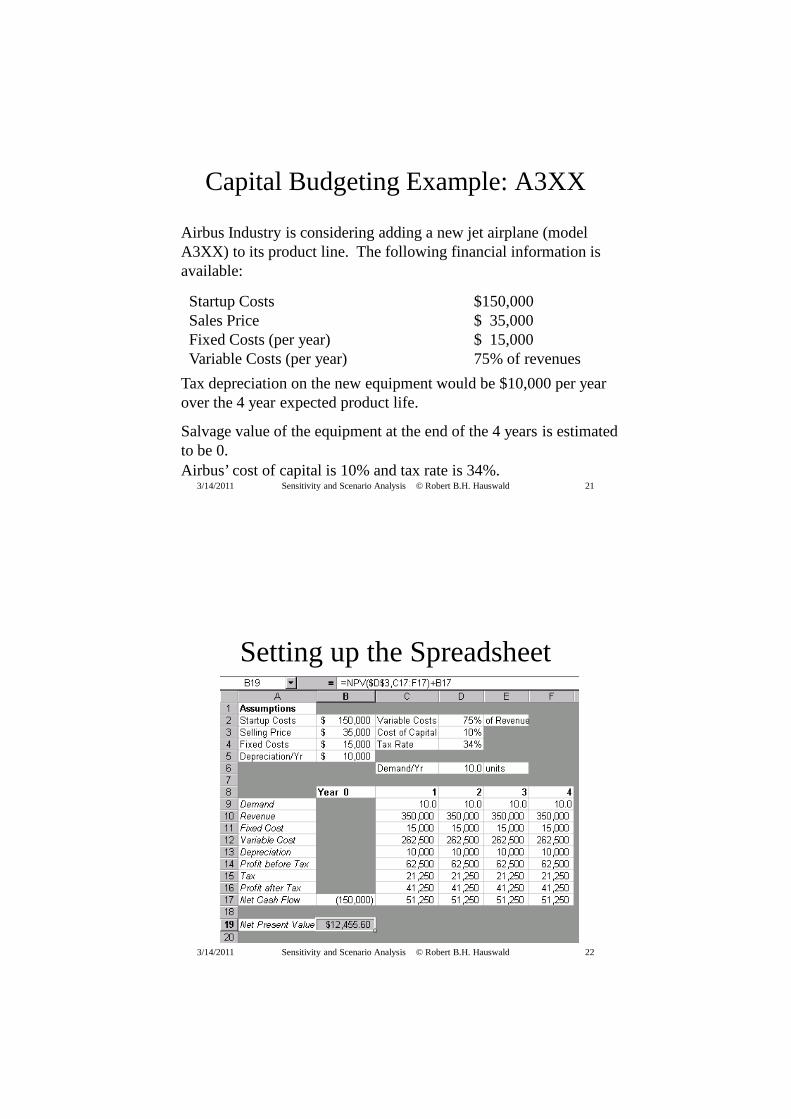
Airbus Industry is considering adding a new jet airplane (model A3XX) to its product line. The following financial information is available:

Startup Costs $150,000Sales Price $ 35,000Fixed Costs (per year) $ 15,000Variable Costs (per year) 75% of revenues

Tax depreciation on the new equipment would be $10,000 per year over the 4 year expected product life.

Salvage value of the equipment at the end of the 4 years is estimated to be 0.Airbus’ cost of capital is 10% and tax rate is 34%.

Capital Budgeting Example: A3XX


Setting up the Spreadsheet


If demand is known, then a spreadsheet can be used to calculate the net present value(NPV). For example, assume that the demand for A3XXs is 10 units for each of the next 4 years

=C9*$B$3=$B$4

=C10*$D$2=$B$5

=C10-SUM(C11:C13)=$D$4*C14=C14 – C15=C16 + C13

=-$B$2

=NPV($D$3,C17:F17)+B17

Formula Details


To model a discrete uniform distribution of demand where the values of 8 through 12 all have the same probability of occurring

The spreadsheet has a function, =RAND(), that returns a random number between 0 and 1. However, this will result in a continuous uniform distribution.To create a discrete uniform distribution, use the INT() function. For example:

In general, if you want a discrete, uniform distribution of integer values between x and y, use the formula:INT(x + (y – x + 1)*RAND())

Uniform Random Variables


It is unlikely that demand will be the same every year; in a more realistic model demand each year is a sequence of random variables.

In this model of demand a constant base level of demand that is subject to random fluctuations from year to year.

Sampling Demand with a Spreadsheet: Assume initially that the demand in a year will be either 8, 9, 10, 11, or 12 units with each value being equally likely to occur.

This is an example of a discrete uniform distribution.

Now, use the formula =INT(8 + 5*RAND() ) to sample from a discrete uniform distribution on the integers 8, 9, 10, 11, 12 .

Multiple trials can be performed by pressing the recalculation key for the spreadsheet (e.g., F9).

Modeling Demand for Airbus


=INT(8+5*RAND() )

Hitting the F9 key would result in a different sample of demands, and possibly a different NPV.

The demands are random variables, therefore, the NPV is also a random variable.


Two key questions need to be answered about the NPV distribution:

1. What is the meanor expected value of the NPV? Statistics?

2. What is the probability that the NPV assumes a negative value (making the proposal to add the A3XX less attractive)?

To answer these questions, a simulation model must be built. To run the simulation automatically and capture the resulting NPV in a separate spreadsheet, use the Data Tablecommand.

Set Calcuations to Manual (F9) to speed up XLS.

Evaluating the Project


Start with a blank worksheet by clicking on the Insertmenu and select Worksheet

Next, rename this blank worksheet 100 Iterations

The Simulation Spreadsheet


Type the starting value (1) in cell A2 and hit Enter, then return to cell A2.

Click the Edit menu and choose Fill – Series.

In the resulting dialog, select Series in Columnsand enter a stop value of 100. Click OK to fill series.

Creating the Data Table


Add column titles and the following formula to cell B2; IRR would be in the C col.

Now select the range A2:B101 and click Data – Table.

Defining the Data Table


In the dialog, enter C1 (D1 with IRR) for the column input cell and click OK.

Note that since a random number generator is used in the formula, you should get different values than those on the right.

Excel recalculates the values and stores the resulting NPV in the adjacent cells in column B (Col input cell: always adjacent to right-most output col).

Running the Simulation


To turn the formulae into actual values first select the range of cells B2:B101, then right-click or select the Edit – CopymenuNext, select the upper left cell of your output range (new worksheet, same columns) and select the Edit – Paste Specialmenu option (or simply right-click the cell) and in the resulting dialog, choose Values.

Saving the Output


To get a summary of the 100 iterations, use Excel’s built-in data analysis tool. Click on Tools – Data Analysis.

If you do not have this option, click on the Add-inoption on the Toolsmenu and in the resulting dialog, click on Analysis ToolPak. After clicking OK, the Data

Analysisdialog will open.

Select the Descriptive Statistics option and click OK.

Analyzing the Output


In the resulting dialog, choose the Input Range

to include the 100 iterations.

Now click on Output Rangeand enter the cell where the output will be placed.

In addition, select Summary Statisticsand click OK.

Descriptive Statistics


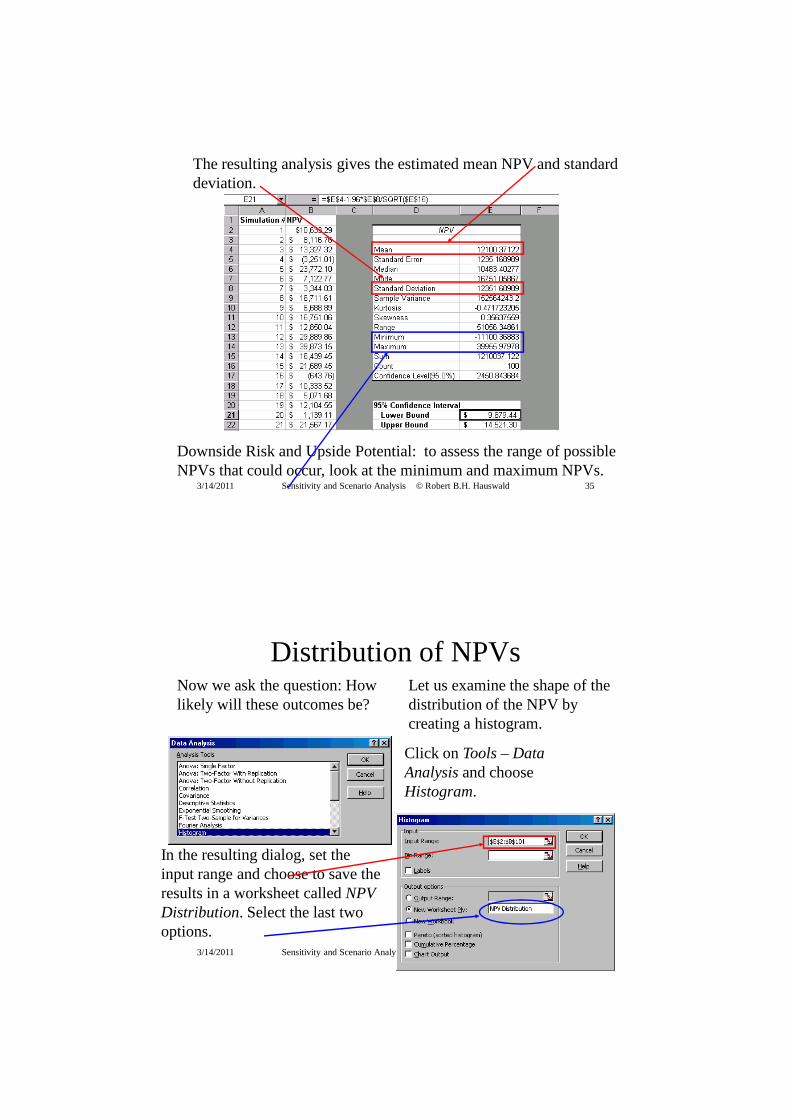
The resulting analysis gives the estimated mean NPV and standard deviation.

Downside Risk and Upside Potential: to assess the range of possible NPVs that could occur, look at the minimum and maximum NPVs.


Now we ask the question: How likely will these outcomes be?

Let us examine the shape of the distribution of the NPV by creating a histogram.

Click on Tools – Data Analysisand choose Histogram.

In the resulting dialog, set the input range and choose to save the results in a worksheet called NPV Distribution. Select the last two options.

Distribution of NPVs


In the resulting analysis, the Frequency(column B) indicates the number of trials that fell into the bins (categories) defined by column A.

The cumulative % column indicates the cumulative percentage of observations that fall into each category or bin.

Frequencies of NPV Realizations


The histogram gives a visual representation of the distribution of NPVs. Note that it is somewhat bell shaped: implies what?

Histograms


Recall our two questions about the distribution that we now can answer together with other statistical information:

1. What is the meanor expected value of the NPV?

2. What is the probability that the NPV assumes a negative value (making the proposal to add the A3XX less attractive) defining the project’s VaR?

In this trial, the mean is $12,100. Standard deviation?

In this trial, the probability is > 15%.

Value-at-Risk: VaR


The next set of questions concerns the faith we put into the simulation: how reliable are the results?

1. How much confidence do we have in the answers from the first trial?

2. Would we be more confident if we ran more trials?

Confidence Intervals

For a 95% confidence interval, the formula is:

estimated mean +1.96(standard deviation)


In our case, the standard deviation is the standard error: the standard deviation divided by the square root of the number of trials.

Based on this trial, the upper and lower confidence limits are:

=$E$4-1.96*$E$8/SQRT($E$16)

=$E$4+1.96*$E$8/SQRT($E$16)

So, we have 95% confidence that the true mean NPV is somewhere between $9,679 and $14,521.

Computing Confidence Intervals


Conclusion

• Simple example how to use XLS for simulation: two crucial commands– RAND(): can be used to model all distributions– Data Table: let XLS automatically generate and store

realizations– Myerson’s SIMTOOLS extend these functions

• Instructive but cumbersome to use– rely on XLS add-ins instead: INFRISK, @Risk,

SIMTOOLS or Crystal Ball– automate simulations and their statistical analysis


Monte Carlo in Perspective

• Monte Carlo analysis of capital-budgeting decisions is a step beyond either sensitivity analysis or scenario analysis

• Interactions between the variables are explicitly specified in Monte Carlo analysis– at least theoretically, this methodology provides a

more complete analysis

– pharmaceutical industry has pioneered applications of this methodology

– its use in other industries is far from widespread


Self-Interested Management

• Managers face conflicts of interest that often destroy project value– career concerns, appropriation of benefits

– can distort information to serve own interests


Conclusions and Generalizations

• It is not appropriate to value earnings, per se – take into account fixed assets and working capital required to

support the sales and generate the earnings.

• Discounted cash flow analysis is not short term– NPV depends on the discount rate used to value the future cash

flows; it properly takes into account long term cash flows.

• Consider economic questions which emphasize change in assessing a company's performance– operating strategies: has the company lowered price to gain a

future payoff (Airlines?)– if a large portion of cost is fixed: future scale economies?– how to value management and strategy (intangibles): beyond the

scope of this class


Assignment

• Add IRR as second output variable and col – Column input cell in Data Table is now: D1

• Random variable cost: uniform• Random fixed cost: lognormal • Random investment amount: uniform• 1,000 iterations• 5,000 iterations• Automate data analysis: hard

advanced cash flows in the npv framework · – asset or resource value if sold rather than used 4....

Documents