Advanced Planning and optimizer – Supply Network Planning

Supply Network Planning

APO Supply Network Planning (SNP) integrates purchasing, manufacturing, distribution, and transportation so that comprehensive tactical planning and sourcing decisions can be simulated and implemented on the basis of a single, global consistent model. Supply Network Planning uses advanced optimization techniques, based on constraints and penalties, to plan product flow along the supply chain. The result is optimal purchasing, production, and distribution decisions; reduced order fulfillment times and inventory levels; and improved customer service.

Starting from a demand plan, Supply Network Planning determines a permissible short- to medium-term plan for fulfilling the estimated sales volumes. This plan covers both the quantities that must be transported between two locations (for example, distribution centre to customer or production plant to distribution center), and the quantities to be produced and procured. When making a recommendation, Supply Network Planning compares all logistical activities to the available capacity.

The Deployment function determines how and when inventory should be deployed to distribution centers, customers, and vendor-managed inventory accounts. It produces optimized distribution plans based on constraints (such as transportation capacities) and business rules (such as minimum cost approach, or replenishment strategies).

The Transport Load Builder (TLB) function maximizes transport capacities by optimizing load building.

In addition, the seamless integration with APO Demand Planning supports an efficient S&OP process.

Integration with Other APO Applications

To... Do this... Other Information

Set up the Supply Chain Model

Use the Supply Chain Engineer (SCE)

In the SCE, you assign the locations, products, resources, and PPMs to a model. You then add transportation lanes to link supply to demand locations, allocate products to the transportation lanes, and maintain quota arrangements.

Make the unconstrained forecast available in Supply Network Planning

Release the Demand Plan to Supply Network Planning and vice versa.

The supply chain planner can then plan resources based on a full and reliable picture of demand, and, likewise, the demand planner can later monitor where adjustments to the demand plan have been necessary due to production, distribution and other constraints.

Make the Supply Network Plan available to PP/DS

Convert the SNP orders into PP/DS orders

In PP/DS, production planning is synchronized with execution to resolve all constraints and bottlenecks and create a viable production plan.

Features

Supply Network Planning is used to calculate quantities to be delivered to a location in order to match customer demand and maintain the desired service level. Supply Network Planning includes both heuristics and mathematical optimization methods to ensure that demand is covered and transportation, production, and warehousing resources are operating within the specified capacities.

The interactive planning desktop makes it possible to visualize and interactively modify planning figures. You can present all key indicators graphically. The system processes any changes directly via live Cache.

Supply Network Planning Process

You use Supply Network Planning (SNP) to model your entire supply network including all associated constraints. You can use this model to synchronize activities and plan the flow of material along the supply chain. This allows you to create feasible plans for purchasing, manufacturing, inventory, and transportation, and to closely match supply and demand.

Process

The following diagram shows the SNP cycle and the integration of SNP with the other components of SAP APO.

The sequence of the process steps described here is generally the sequence in which you should carry out the cycle. However, you may need to repeat certain steps or to proceed in a different order. Also, not all activities are mandatory.

Page 1 of 251

Advanced Planning and optimizer – Supply Network Planning

Planning Area Administration

Take all the necessary steps to set up your planning area. The planning area is the basis for all activities in SNP. It is a collection of parameters that define the scope of all planning tasks.

SAP APO Master Data Setup

Master data is a crucial aspect of the SNP component in SAP APO. You have to configure this master data very carefully to achieve satisfactory results. SNP master data includes information about locations, products, resources, production process models (PPMs) or production data structures (PDS), and transportation lanes.

Model/Version Creation

Before you set up the model in the Supply Chain Engineer (SCE), you have to create a model name and assign the model to at least one version. You can assign the model to several different versions for simulation purposes. The version is also used for releasing the demand plan (final forecast) to SNP and for releasing the supply network plan to Demand Planning.

Supply Chain Model Setup

You set up the supply chain model for SNP in SCE. There you assign the locations, products, resources, and PPMs or PDS to a model. You then add transportation lanes to link supply locations to demand locations, allocate products to the transportation lanes, and define quota arrangements.

Release Forecast Data to SNP

You release forecast data to SNP by first loading the data in a planning area in demand planning (DP) and then releasing it, or by directly releasing it from an Info Provider. The data is often unconstrained by any production or distribution restrictions. Either the demand planner or the SNP planner can execute this step.

Page 2 of 251

Advanced Planning and optimizer – Supply Network Planning

Definition of Planning Method and Profile Settings

You choose whether you want to use optimization-based planning, heuristic-based planning, or supply and demand propagation as your planning method. You also decide if you want to perform safety stock planning before the Supply Network Planning run. You then make the settings in the appropriate profiles for each of the methods requiring settings. You can still change these profiles during planning for simulation purposes. You may need to define additional master data specifically for the method you are using.

Supply Network Planning Run

You perform the planning run once you have chosen the method and carried out the prerequisite steps.

The result of a Supply Network Planning run using the heuristic, the optimizer, supply and demand propagation, or Capable-to-Match is a medium-term production and distribution plan.

Interactive Planning

After the SNP run, you review the plan in the interactive planning desktop. If you run heuristic-based planning, you can also level capacities from the interactive planning table.

Release SNP Plan to DP

You release the final supply network plan back to Demand Planning (DP) to compare the demand plan (without constraints) with the constraint-based supply network plan. Major discrepancies between these two plans could trigger re-forecasting, and, ultimately, re-planning. For example, you may want to release the supply network plan back to DP if the capacity situation is not sufficient to fulfill demand created by a promotion and you need to make adjustments to the promotion planning strategy.

Converting SNP Orders into PP/DS Orders

This is not part of the SNP process since it can only be done in Production Planning and Detailed Scheduling (PP/DS). However, it is included in the cycle because this step is usually performed before running deployment and the Transport Load Builder.

In PP/DS, you convert SNP orders into PP/DS orders to make them available for Production Planning and Detailed Scheduling.

Production Planning and Detailed Scheduling (PP/DS)

This is not part of the SNP process because it can only be run in PP/DS. However, it is included in the cycle because Production Planning and Detailed Scheduling is usually run before deployment and the Transport Load Builder, which are both part of the Supply Network Planning application component.

In PP/DS, you create a viable production plan based on the planned orders generated in SNP.

Deployment Run

After production planning is complete and the system knows what will actually be produced (this information is saved automatically in liveCache), the deployment run generates deployment stock transfers.

Transport Load Building

The Transport Load Building (TLB) run groups the deployment stock transfers resulting from the deployment run into TLB shipments. You can also manually create TLB shipments for stock transfers that could not be taken into account during the TLB run due to specified constraints.

Planning Area Administration

The set up of the Supply Network Planning (SNP) system environment is integral to successful planning. Planning area administration is the first step in this setting-up process?

Prerequisites

You have understood the differences between the different storage methods in Supply Network Planning and Demand Planning, and know which functions are supported by which storage methods. For more information, see Data Storage in Supply Network Planning and Demand Planning.

You have understood the role and purpose of the following:

Key Figure

Characteristic

Master Planning Object Structure

Storage Buckets Profile

Planning Area

Planning Book

Page 3 of 251

Advanced Planning and optimizer – Supply Network Planning

Note that the attribute object (navigation attribute for instance) is only used in Demand Planning. You cannot create aggregate objects yourself, as opposed to Demand Planning, where you can do this. If you create and activate your own master planning object structure (see step five below), SNP aggregates are generated automatically.

Process

1. For Supply Network Planning, SAP delivers pre-defined standard key figures and characteristics, which mean you, do not have to create your own key figures and characteristics. The characteristics in master planning object structure 9ASNPBAS and key figures in the planning areas 9ASNP01, 9ASNP02, 9ASNP03, or 9ASNP04 are displayed in Administration of Demand Planning and Supply Network Planning (APO Easy Access menu → Supply Network Planning → Environment → Current Settings → Administration of Demand Planning and Supply Network Planning). If you do not see these key figures and characteristics there, go to the ABAP Editor to create them in your system (APO Easy Access Menu → Tools → ABAP/4 Workbench → Development → ABAP Editor) and run the program /sapapo/ts_d_objects_copy.

If the key figures that are delivered with the system are not sufficient for your purposes, you can create additional key figures in the Administrator Workbench (from Administration of Demand Planning and Supply Network Planning, choose Administrator Workbench and then Tools ® Edit Info Objects). If the system asks you to choose between an APO key figure and a BW key figure, choose APO key figure. When creating a key figure for quantities, select Quantity and enter the data type QUAN and the unit 0BASE_UOM or 0Unit.

2. You create storage bucket profiles from SNP Current Settings by choosing Periodicities for Planning Area. For more information, see Storage Buckets Profile.

3. You create planning bucket profiles in Customizing from Supply Network Planning by choosing Define planning bucket profiles. For more information, see Planning Buckets Profile.

4. You create the planning versions that you want to use for SNP and assign them to a supply chain model. For more

information, see Model/Version Creation.

5. SNP comes with the standard master planning object structures 9ASNPBAS and 9ASNPSA (for scheduling agreement processing). You also have the option of creating your own master planning object structure. However, this does not have any advantages over using the standard master planning object structures. To create a new master planning object structure, from the SAP Easy Access screen, choose Supply Network Planning → Environment → Current Settings ® Administration of Demand Planning and Supply Network Planning. Then, from the top left pull-down menu Administration, choose Planning Object Structures, right-click the Planning Object Structures folder, and choose Create Planning Object Structure. If you select the SNP Planning indicator, the SNP standard characteristics are adopted into the master planning object structure automatically.

It is not possible to use additional characteristics in SNP. The delivered standard characteristics mentioned above should not be changed either. In particular, you are not permitted to add navigation attributes to characteristics, as SNP does not support them (apart from the standard navigation attributes), which means that using navigation attributes leads to problems.

When you activate the master planning object structure, you are asked whether you want the SNP standard planning level to be created. Confirm this to trigger generation of the SNP aggregates (that is, master data objects such as location product or resource). You also still have the option of creating the SNP standard planning level at a later point in Administration of Demand Planning and Supply Network Planning using the context menu function from the master planning object structure.

For more information, see Master Planning Object Structure and IMG.

6. SAP delivers the following standard planning areas for SNP:

9ASNP01 (time series-based)

9ASNP02 (order-based)

9ASNP03 (for scheduling agreement processing)

9ASNP04 (for optimization-based planning with time-dependent restrictions)

9ASNP05 (for safety stock planning)

9AVMI03 (for deployment heuristic with consideration of demands in the source location)

You can also create your own planning areas: From the SAP Easy Access screen, choose Supply Network Planning → Environment → Current Settings ® Administration of Demand Planning and Supply Network Planning, and choose Planning Areas from the pull-down menu Administration on the top left.

To create an order-based SNP planning area, you should copy an order-based SNP standard planning area. That way you can ensure that your own planning area contains the entire key figures with their necessary attributes required in SNP. To create a time-series-based SNP planning area, you should choose menu function Edit ® SNP Time Series Object, which adds the standard SNP time series key figures to the planning area. You can also assign additional key figures to your planning area to store data that is calculated by a macro, for example. Note that you should not make any

Page 4 of 251

Advanced Planning and optimizer – Supply Network Planning

settings for the additional key figures in the key figure details since these key figures would then be created in liveCache time series objects.

For more information, see Planning Area and IMG.

7. You set up your master data for SNP. For more information, see Master Data for Supply Network Planning.

8. You initialize the planning area by right-clicking the planning area and choosing Initialize Planning Version. Note that the context menu function for initializing is only called Initialize Planning Version if no time series key figures are included in the planning area. If at least one of these key figures exists in the planning area, the context menu function is called Create time series objects.

If you need to re-initialize a planning area after updating your master data or in order to extend the planning horizon, you do not need to de-initialize it first or delete the time series objects. The system recognizes new and deleted planning objects and updates accordingly.

6. Create planning books and planning views. You can assign the planning books and planning views to individual users. For more information, see Planning Book.

SNP provides the following standard planning books and data views for the different types of planning. For SNP, we recommend that you use these standard-planning books. If you need to create additional planning books, you should use the standard books as templates.

9ASNP94 (Interactive Supply Network Planning and Transport Load Builder (TLB)) - This planning book offers the

standard functions for running interactive Supply Network Planning and the interactive Transport Load Builder.

9ASOP (Sales & Operations Planning (SOP)) - You use this planning book to run SNP planning method supply and demand propagation.

9ADRP (Distribution Resource Planning (DRP)) – This user interface is almost identical to the interactive Supply Network Planning interface, the only difference being that here it is also possible to display distribution receipts and issues.

9AVMI (Interactive VMI) - In addition to the typical SNP data that you can display, you can also display the values for your VMI receipts and demands (planned, confirmed, and TLB-confirmed).

9ASA (interactive scheduling agreements) – You use this planning book to display and change all data that is

relevant for scheduling agreement processing.

9ASNPAGGR (Aggregated Planning) – You use this planning book to perform aggregated planning and planning with aggregated resources.

9ASNP_PS (product interchangeability) – You use this planning book if you want to consider product interchangeability when planning.

9ATSOPT – You use this planning book to define time-based constraints for optimization-based planning.

9ASNP_SSP – You must use this planning book (or one based on it) if you want to apply certain standard safety

stock planning methods. You can also use this book for extended safety stock planning.

9DRP_FSS – You can use this planning book (or one based on it) if you want the deployment heuristic to also

consider customer demands or planned independent demands in the source location. For more information, see Consideration of Demands in the Source Location.

Master Planning Object Structure

Definition

A master planning object structure contains plannable characteristics for one or more planning areas. In Demand Planning, the characteristics can be either standard characteristics and/or ones that you have created yourself in the Administrator Workbench. Characteristics determine the levels on which you can plan and save data. Specific characteristics are required for Supply Network Planning, Characteristics-Based Forecasting and forecasting of dependent demand; these characteristics can be included on demand in the master planning object structure.

The use of additional characteristics for Supply Network Planning is not supported. For an example of a master planning object structure with the correct characteristics for Supply Network Planning, see 9ASNPBAS.

The master planning objects structure is the structure on which all other planning object structures are based. Other planning object structures are aggregates and standard SNP planning levels.

A master planning object structure forms part of the definition of a planning area. The existence of a master planning object structure is therefore a prerequisite for being able to create a planning area.

Integration

Page 5 of 251

Advanced Planning and optimizer – Supply Network Planning

Before you can start planning, that is entering data for key figures; you must have created characteristic combinations. You do this for each master planning object structure.

Working with Master Planning Object Structures

Master planning object structures are prerequisites for creating planning areas in Supply and Demand Planning.

In Demand planning you can assign any characteristics that exist in the system to the master planning object structure.

The following applications have fixed sets of standard characteristics:

Supply Network Planning

Characteristic-based forecasting

Forecasting with bills of material

Prerequisites

You have created the characteristics with which you wish to work.

Procedure

To edit master planning object structures you work in Supply and Demand Planning Administration, which you access by choosing Demand Planning/Supply Network Planning → Environment → Current Settings → Administration of Demand Planning and Supply Network Planning.

In S&DP Administration you can edit:

Planning areas

Master planning object structures

To edit master planning object structures choose Planning object structures on the selection button (top left of the screen).

Creating Master Planning Object Structures

1. Choose Create master planning object structure from the context menu.

2. On the dialog box that appears enter a name for the new master planning object structure and choose . The Configure Planning Object Structure screen appears.

3. Enter a descriptive text for the master planning object structure.

4. You now assign characteristics from the table on the right of the screen. If the master planning object structure is for use in one of the applications listed above in the Use section, simply select the relevant indicator. The standard characteristics are transferred automatically. Otherwise select the characteristics that you want to use and then choose

. Similarly you can choose to remove characteristics from the master planning object structure.

5. You can also assign dimensions to the characteristics in your master planning object structure. Dimensions here are similar to dimensions in InfoCubes and are used to improve performance. To assign dimensions use the pull-down box

in the dimension ( ) column of the left hand table. You can add further dimensions by choosing the Add button at the bottom of the screen.

6. If you want to use other characteristics for product and location than 9AMATNR and 9ALOCNO, you must specify these characteristics in the master planning object structure. In general you should use the two SAP characteristics as the basis for the new characteristics. The main reason for changing these characteristics is to be able to use navigational attributes in Demand Planning without causing problems afterwards in SNP (SNP does not support navigational attributes). To assign the product / location characteristics in the master planning object structure choose Edit → Assign prod. /loc. Enter the relevant characteristics in the dialog box that appears.

7. Save your master planning object structure.

Changing Planning Object Structures

SAP recommends that you do not change master planning object structures that have been activated and that are in use in planning books.

To remove a characteristic from a master planning object structure you must first deactivate the structure.

When you deactivate a master planning object structure, all characteristic value combinations are deleted and the existing liveCache time series objects become inconsistent.

Activating/Deactivating Master Planning Object Structures

Before you can work with a master planning object structure (for example create characteristics combinations or assign them to a planning area) you must activate it.

You can do this either:

Page 6 of 251

Advanced Planning and optimizer – Supply Network Planning

From the planning object structure workspace in S&DP Administration by selecting the master planning object structure and then choosing Activate or Deactivate from the context menu.

On the Configure Planning Object Structure screen by choosing to activate or to deactivate.

Read the cautions above before deactivating master planning object structures.

Storage Buckets Profile

There are two kinds of time bucket profiles: one is used for storing data (the storage buckets profile), and the other for planning the data (the planning buckets profile).

A storage buckets profile defines the time buckets in which data based on a given planning area is saved in Demand Planning or Supply Network Planning.

In a storage buckets profile, you specify:

One or more periodicities in which you wish the data to be saved

The horizon during which the profile is valid.

You can also include a time stream in storage bucket profile. You use time streams to incorporate factory calendars and other planning calendars in Demand Planning. You can thus specify which days are workdays and which days are holidays. You define time streams in Customizing under APO → Master Data → Calendar → Maintain Planning Calendar (Time Stream). Refer to the implementation guide (IMG) before editing time streams.

You assign the time stream to the storage bucket profile in the relevant field at the bottom of the screen.

You select the periodicities month and week in the storage buckets profile. You do not enter a time stream. Data for the months of June and July 2001 is stored in the following buckets, also known as technical periods.

Time span Number of days

Friday through Sunday, June 1-3 3 days

Monday through Sunday, June 4-10 7 days

Monday through Sunday, June 11-17 7 days

Monday through Sunday, June 18-24 7 days

Monday through Saturday, June 25-30 6 days

Sunday, July 1 1 days

Monday through Sunday, July 2-8 7 days

Monday through Sunday, July 9-15 7 days

Monday through Sunday, July 16-22 7 days

Monday through Sunday, July 23-29 7 days

Monday and Tuesday, July 30-31 2 days

The definition procedure for storage bucket profiles is the same for Demand Planning and Supply Network Planning.

Include in the storage buckets profile only the periodicities you need because the technical periods take up storage space. On the other hand, you must include all the periodicities in which you intend to plan. For example, if you intend to plan in months, you must include the periodicity month in the storage buckets profile.

You need a storage buckets profile before you can create a planning area.

The storage buckets profile can be used for the release to SNP. For more information, see Release of the Demand Plan to SNP.

The way data is saved is further defined by the way you customize the Calculation type and Time-based disaggregation

in the planning area. For more information, see Aggregation and Disaggregation and the F1 Help for these fields.

To define the buckets in which data is displayed and planned in interactive planning, create a planning buckets profile. For more information, see Planning Buckets Profile.

You maintain storage bucket profiles in Customizing under Supply Chain Planning → Demand Planning → Basic Settings → Define Storage Bucket Profile.

Once a storage buckets profile is in use, it is not possible to change it. It is therefore sensible to specify a relatively long horizon. Since the storage bucket profile does not take up any room in liveCache, this does not affect performance.

Page 7 of 251

Advanced Planning and optimizer – Supply Network Planning

Planning Buckets Profile

Information, which is incorporated into the definition of the past or future time horizon of demand planning. The planning buckets profile defines the following:

Which time buckets are used for planning

How many periods of the individual time units are used

The sequence in which the time periods with the various time units appear in the planning table

Use

You can plan in monthly, weekly, daily or (combined with fiscal year variants) self-defined periods.

When you create a planning buckets profile, only use the periodicities or a subset of the periodicities that are also defined in the storage buckets profiles (see storage buckets profiles) on which the planning area is based. In a planning buckets profile, do not include a periodicity that is not in the storage buckets profile.

You can have multiple planning buckets profiles, and therefore multiple planning horizons, for one planning book. The planning buckets profile is attached to the data view within the planning book. You could have three data views for three users, for example, where a different planning buckets profile is valid for each view: Marketing plans in months, sales plans in months and weeks, and logistics plans in weeks and days.

To switch to a different planning buckets profile in interactive planning, you open the planning book wizard by changing to Design mode and choosing the Change Planning Book button. On the Data View tab page, enter a name and description for the new view as well as the required time bucket profiles and any other necessary data.

If you specify a historical planning horizon in the data view, the first historical time bucket starts on the day before the future planning horizon start date. The second historical period begins further back in the past, and so on. If you plan in weeks, the first day of the week is always Monday.

If you plan in weeks and the planning horizon start date as specified in the data view of the planning book is not a Monday, the first week of the planning horizon is predated to the previous Monday. For example, if the planning horizon starts date as specified in the planning book is November 1, 2001 (a Thursday), the first week of the planning horizon begins on October 29, 2001 (a Monday).

If the planning buckets profile contains smaller and larger time buckets, for example weeks and months, the smaller time buckets take precedence if any conflict arises. If, for instance, you have specified that the first month is to be planned in weeks and the month does not start or end on a Monday, the system creates 5 time buckets of a week's duration. For example, you start planning on January 01, 2001 and specify that the first month (January) is to be planned in weeks. The first 5 time buckets from January 1 to February 4 are in weeks. The first month bucket is shortened and is from February 5 through February 28.

If you forecast using mass processing jobs, the length of the planning horizon is a vital prerequisite for being able to save corrected history and the corrected forecast. The historical planning horizon in the planning book must include the historical forecast horizon in the master forecast profile. It may also go further back into the past than the historical forecast horizon in the master forecast profile. It must not be shorter than in the master forecast profile. Similarly, the future-planning horizon in the planning book must include the future forecast horizon that is defined in the master forecast profile. It may also extend further into the future than the future forecast horizon in the master forecast profile. It must not be shorter than in the master forecast profile. This restriction is necessary for performance reasons. It does not apply if you forecast in interactive demand planning.

To read the data for the online release of the demand plan to SNP, you can use a planning buckets profile. For more

information, see Release of the Demand Plan to SNP.

To release the demand plan to Supply Network Planning in daily buckets, you use a daily buckets profile, that is a planning buckets profile containing daily buckets only. The use of a time buckets profile to release data to Supply

Network Planning is optional. See also Release of the Demand Plan to SNP and Release from an Info Provider to SNP.

To see the start and end dates of a period in a planning book or in the demand-planning table, double-click with the right mouse button on the column heading. In this dialog box, you can also configure what information you want to see in the column heading.

The buckets in which the data is stored in the system are known as storage buckets or technical periods. You define these technical periods when you create a storage buckets profile. For information on how technical periods affect

disaggregation and rounding, see Example of Disaggregation and Rounding.

Structure

After you have created the planning buckets profile, use it for the definition of the future planning horizon and of the past horizon by entering them in a planning book: one horizon as future planning horizon and one as past horizon. The system displays the horizons in interactive demand and supply planning starting with the smallest time bucket and finishing with the

Page 8 of 251

Advanced Planning and optimizer – Supply Network Planning

largest time bucket. The future horizon starts with the smallest time bucket; on the planning horizon start date, and works forwards, finishing with the largest time bucket. The past horizon starts with the smallest time bucket the day before the start of the future horizon and works backwards, finishing with the largest time bucket:

Example

Number of periods

Basic periodicity

Fiscal year variant of basic periodicity (optional)

Display periodicity

Fiscal year variant of display periodicity (optional)

2 Y

1 Y M

2 M W

In the above example, the time horizon spans two years. Of these two years, the first year is displayed in months. The first two months of this year are displayed in weeks.

The first row defines the entire length of the time horizon. The following rows define the different sections of the horizon. You make entries in the columns Number and Display periodicity. The content of the other columns is displayed automatically when you press Enter. To see exactly which buckets will be displayed, choose Period list.

Key Figure

Contains data that is represented as a numerical values either a quantity or a monetary value. Examples of key figures used in Demand Planning are planned demand and actual sales history. Examples of key figures used in Supply Network Planning are production receipts and distribution receipts.

You create key figures in the Administration Workbench, even if you only intend to use the key figures in LiveCache. Choose Tools, Edit Info Objects.

In APO, create APO key figures (not BW key figures).

There are three types of key figure that are of interest for demand planning:

Quantity- Use this type for physical quantities

Amount - This type is amounts of money

Number - Use this type for numbers that do not have units of measure or currencies, such as factors.

The unit of measure and currency are always taken from the planning area.

There are different places in which a key figure can be stored. For detailed information, see Data Storage in Demand Planning and Supply Network Planning.

Characteristic

A planning object such as a product, location, brand or region.

The master data of Demand Planning or Supply Network Planning encompasses the permitted values of the characteristics, the characteristic values. Characteristic values are discrete names or numbers. For example, the characteristic 'location' could have the values London, Delhi and New York.

The characteristics used in Demand Planning are the same as those used in the SAP Business Information Warehouse. You

create and edit characteristics in the Administration Workbench. For more information, see InfoObject and Creating InfoObject: Characteristics.

SAP delivers several characteristics for use in SAP APO as Business Content. These characteristics have the prefix 9A as opposed to 0 for other BW characteristics. As SAP reserves the right to change these characteristics without notice, we strongly recommend that you do not change them.

Compared to BW characteristics there are the following restrictions for the use of characteristics in Demand Planning.

Data types DATS – Date and TIMS – Time are not permissible.

Similarly lowercase characteristic names are not permissible. (You can of course use lowercase in the description fields.

We recommend that you do not use compound characteristics.

Page 9 of 251

Advanced Planning and optimizer – Supply Network Planning

Planning Area

Planning areas are the central data structures for Demand Planning and Supply Network Planning.

The planning area is created as part of the Demand Planning/Supply Network Planning setup. A planning book is based on a planning area. The end user is aware of the planning book, not the planning area. The liveCache objects in which data is saved are based on the planning area, not the planning book.

The planning area specifies the following:

Unit of measure in which data is planned

Currency in which data is planned (optional)

Currency conversion type for viewing planning data in other currencies (optional)

Storage buckets profile that determines the buckets in which data is stored in this planning area

Aggregate levels on which data can be stored in addition to the lowest level of detail in order to enhance performance

Key figures that are used in this planning area

Settings that determine how each key figure is disaggregated, aggregated, and saved

The assignment of key figures to aggregates

Supply Network Planning comes with predefined planning areas. You can also define your own planning areas.

You define planning areas in S&DP Administration.

Structure

You assign a planning area to a master planning object structure, which in turn is assigned characteristics and aggregates, which in turn are assigned characteristics and aggregates.

You assign the key figures with which you want to work directly to the planning area.

Mass Maintenance of Time Series Key Figures

In Supply Network Planning (SNP), planning is generally based on order key figures. However, in some areas, you can also

use time series key figures, for defining time-dependent restrictions for optimization-based planning, for instance.

You can use this function to carry out mass maintenance of time series key figures, that is, you can select several key figures and planning objects, and either define the key figure values for individual periods, or for all periods.

You can also use this function to process time series key figures for Demand Planning (DP).

Features

Selection of Key Figures

You can select the key figures for a particular planning area and planning time period, as well as for particular planning objects. As when defining a planning book, you determine the planning time period and the period schedule lines, by entering a planning buckets profile and a planning start date. You can also shorten the planning time period further by entering a time period for maintenance.

You select the planning objects with the shuffler, as in interactive planning. In addition to the standard planning objects, in this function, you can also use the SNP aggregate APO – Product Transport (a product on a transportation lane). The APO – PPM/PDS aggregate also includes the header product for the production process model (PPM) or the production

data structure (PDS). If you select Display Selected Objects,

Definition of Key Figure Values

You can define key figure values for individual periods or for all periods. The options available are:

Set Key Figure Values: You can define the values for the individual periods. You can use the distribution function to distribute values over periods, as in interactive planning.

Change Key Figures: You can define or change the values for all periods in the planning time period. You can also determine, for example, that you want the system to add or subtract specific values or percentages to (or from) existing values.

Note that values saved earlier or in liveCache are not displayed, but are overwritten by the new values.

Activities

1. Select Advanced Planning and Optimization ® Supply Network Planning ® Environment ® Mass Maintenance of Time Series Key Figures from the SAP Easy Access screen.

2. Select the key figures as detailed above, and then select Set Key Figures or Change Key Figures.

Page 10 of 251

Advanced Planning and optimizer – Supply Network Planning

3. After entering the values, select (with tool tip Save) or (in the Background). If you select the latter option, you carry out the saving procedure as a background job.

Data Storage in Demand Planning and Supply Network Planning

In Demand Planning and Supply Network Planning, you can store data in three ways:

In liveCache time series objects

In liveCache orders

In an InfoCube

Each key figure in a planning area has its own storage method.

Integration

Since planning areas for Supply Network Planning can contain only the standard SNP characteristics, you can only use a joint planning area for Demand Planning and Supply Network Planning, if demand planning in your company is done at product level or at product and location level. If you want to do demand planning at other levels, such as brand or regional level, you must have separate planning areas.

Features

LiveCache Time Series Objects

The data is stored in buckets, with no reference to orders. This storage method is suitable for tactical, aggregated planning. It is the usual method for saving current Demand Planning data. It also supports the Sales & Operations Planning process. If you save a key figure to liveCache time series objects, you can use the following functions:

Constraint propagation up and down stream (material constraints, capacity constraints, stock level constraints)

Aggregation and disaggregation

Freely definable macros

Product allocation checks

Characteristics-Based Forecasting (CBF)

Single- and multilevel infinite heuristics

Capacity leveling

MILP Optimizer

Capable-to-Match

Deployment

Vendor-Managed Inventory (VMI)

There are a number of standard key figures that are saved to liveCache time series objects which you can include in an SNP planning area by choosing Edit → SNP time series objects.

The prerequisites for saving a key figure to liveCache time series objects are that:

You have created time series objects for the planning area.

When creating the planning area, you made no entries for the key figure in the fields InfoCube, Category or Category Group.

When creating the planning area, any entry you made in the field Key figure semantics is prefixed with TS (an entry in this field is optional).

For an example of Sales & Operations Planning using the time series storage method, see planning book 9ASOP, planning area 9ASNP01 (transaction /SAPAPO/SNPSOP) in the standard APO system.

LiveCache Orders

The data is stored with reference to orders. This storage method is suitable for operative planning, such as in a classical SNP setup. If you save a key figure to liveCache orders, you can use the following functions:

Real-time integration with R/3

Full pegging

Freely definable macros

Single- and multilevel infinite heuristics

Capacity leveling

MILP Optimizer

Page 11 of 251

Advanced Planning and optimizer – Supply Network Planning

Capable-to-Match (CTM)

Deployment

One-step deployment

Transport Load Builder (TLB)

Vendor-Managed Inventory (VMI)

There are a number of standard key figures that are saved to liveCache orders which you can include in an SNP planning area by choosing Edit → SNP standard.

The prerequisites for saving a key figure to liveCache orders are that:

You have created time series objects for the planning area (even though you are saving to orders).

When creating the planning area, you either specified a Category or Category Group or entered a Key figure semantic prefixed with LC.

When creating the planning area, you made no entry for the key figure in the field InfoCube.

For an example of Supply Network Planning using the orders storage method, see planning book 9ASNP94, planning area 9ASNP02 (transaction /SAPAPO/SNP94) in the standard APO system.

InfoCubes

The data is stored in an InfoCube in the Administrator Workbench. This storage method is suitable for data backups, old planning data, and actual sales history. In Demand Planning, actual sales history is used to generate master data and as the basis for forecasting.

In APO Demand Planning you can only read from InfoCubes if you have specified the InfoCube in planning area configuration. For details of how to save data to InfoCubes see Exchange of Data Between InfoCubes and Planning Areas.

To specify an InfoCube from which the key figure is read in all versions:

1. Select the planning area in S&DP Administration.

2. Choose Change in the context menu.

3. On the Key figs tab page choose Details.

4. Select the relevant key figure and enter the InfoCube in the relevant field.

It is possible to use different InfoCube for different versions. Continue as above up to step 3. In Step 4 do not enter an

InfoCube. Choose . A dialog box appears, in which you enter the InfoCube for each version. After you entered the

necessary information, choose to save the data and return to the previous screen. You can see that such data has been

entered by the icon.

Extracting Data from a Planning Area

There are two purposes for which you might follow this procedure:

For ad hoc reporting for planning area data

To save data persistently to the database

Procedure

1. Generate an export Data Source for the planning area. To do so, proceed as follows:

a. On the SAP Easy Access screen, choose Demand Planning → Environment → Administration of Demand Planning and Supply Network Planning.

b. Select the planning area and, in the context menu, choose Change/Display.

c. In planning area maintenance, choose Extras → Generate Data Source.

A dialog box appears in which you enter a name for the data source.

d. Choose Execute.

A screen with details for the data source appears.

e. Specify the fields that you want to be able to select later for reporting purposes. This step enables you to limit a query to specific objects or ranges of objects. Your selection here does not influence the fields that are included in the export structure. Select the Suppress field indicator for the fields (InfoObjects) that you do not want to transfer.

The number of fields that you transfer directly affects performance. Therefore, we recommend that you only transfer those fields that you require for reporting purposes in the InfoCube.

Page 12 of 251

Advanced Planning and optimizer – Supply Network Planning

The field for the planning version is selected by default; you cannot deselect it. This means that you must enter a planning version in the InfoPackage later.

f. Make a note of the DataSource name.

g. Choose Save.

2. Replicate the DataSource. To do so, right mouse click the source system and choose Replicate DataSources in the Data Warehousing Workbench. In this case, the source system is the system in which you are performing Demand Planning. For example, if you are planning in the SAP SCM system, client 002, the technical name of the source system is APOCLNT002.

When the system messages at the bottom of your screen cease, a background job is triggered. Check in the job overview that this job has finished before proceeding to the next step.

3. In the Data Warehousing Workbench, you are still in the source system view. Right-click the source system and choose DataSources Overview in the context menu.

4. Assign an InfoSource to the DataSource: To do so, proceed as follows:

a. In the DataSource overview under Data Marts, select the DataSource and choose Assign InfoSource from the context menu.

b. In the dialog box, choose Create.

c. In the next dialog box, enter a name and a short description for the InfoSource.

d. When the InfoSource has been created, choose Enter.

e. Answer the system prompt with Yes.

This saves the InfoSource/DataSource assignment.

If the above procedure is unsuccessful, use the following alternative:

Switch to the InfoSource view.

Create an InfoSource (right-click a suitable InfoArea and choose Create InfoSource).

Right-click the InfoSource and choose Assign DataSource from the context menu.

A dialog box appears with an overview of all DataSources in the Data Mart, including the export DataSources you have generated yourself.

Select the DataSource you created in step 1.

5. In the Data Warehousing Workbench, branch to the InfoSource view.

6. Right-click the InfoSource that you have just created and choose Change.

The screen in which you can specify the assignment of the communication structure to the transfer structure appears. You see the communication structure in the upper half of the screen and the transfer structure in the lower half. Some of the assignment information is proposed by the system. You must fill in the missing information.

This is another opportunity to remove superfluous InfoObjects from the communication structure. See also step 1.

7. Define the assignment of the communication structure to the transfer structure. To do so, proceed as follows:

a. In the lower half of the screen, enter the source system and the DataSource for the transfer structure.

b. On the Transfer Structure tab page, copy the objects from the DataSource to the transfer structure (from right to left).

c. Click the Transfer Rule tab page.

d. Check where the assignment of transfer structure fields to communication structure InfoObjects is not proposed by the system.

e. Where the assignment has not been proposed:

Include new InfoObjects in the communication structure in the upper half of the screen.

In the lower half of the screen, select the new InfoObjects in the communication structure on the left and copy the InfoObjects to the appropriate fields in the transfer structure on the right.

f. Choose Activate.

8. If you need an InfoCube to carry out reporting with a BI front end, create an SAP Remote InfoCube, specifying the InfoSource that you created in step 4 as the InfoSource, Otherwise, see the note below.

9. Activate the SAP Remote InfoCube.

Result

In the SAP Business Explorer Browser, you can now create queries based on this SAP Remote InfoCube. See also Ad Hoc Reporting on Data in a Planning Area

Page 13 of 251

Advanced Planning and optimizer – Supply Network Planning

If you want to copy planning area data to an InfoCube for backup purposes or to save old planning data, create a basic InfoCube during step 8 (for example, by running program /SAPAPO/TS_PAREA_TO_ICUBE) and proceed as you would when uploading data from an ERP system or a flat file.

Tools for Extraction from Planning Areas

SAP provides a group of tools for checking and working with DataSources and other objects used in conjunction with planning areas.

Most of the functions available here are also available in other transactions, in particular in the Data Warehousing Workbench and in Administration of Demand Planning and Supply Network Planning. The data extraction functions described here has been bundled together for ease of use.

DataSource Management

Generate DataSource

You use this function to generate a DataSource. This is the existing SAP APO function that you can also access from the context menu for a planning area under Generate Export DataSource.

You can only create one DataSource for each basis planning object structure and each aggregate assigned to a planning area.

You can choose any characteristic to be used for selection purposes. The characteristic 9AVERSION for the planning version is always used for selection and cannot therefore be changed here. You cannot use key figures or units for selection purposes.

You must enter the version in the selection when you call up the DataSource. Otherwise, the system issues an error message.

You use the Suppress field indicator to exclude key figures from a DataSource. These key figures are not extracted. This reduces the amount of data to be handled, and thus improves performance.

For performance reasons, we recommend that you only use export DataSources for extracting data from liveCache. You can extract key figures from an InfoCube directly by creating an export DataSource in the Data Warehousing Workbench.

For technical reasons, extracting data from planning areas to InfoCubes using DataSources is only possible with full uploads. However, you can use Data Store objects to simply update the changes. For more information, see Updating InfoCubes Using Data Store Objects.

Change/Display DataSource

This function allows you to change or display a DataSource using the same screen as above.

Check DataSource

This function runs a consistency check on the selected DataSource and displays a log if errors are found.

Repair DataSource

This function attempts to repair errors found in the above checks.

Test DataSource

You can use this function to test data extraction using the selected DataSource.

Restrictions

Do not use F4 help.

The system uses the internal representation of characteristic values. This means:

When entering numeric characteristic values, use leading zeros, if necessary

Enter dates in internal formal, that is, YYYYMMDD, YYYYMM, YYYYWW, for example

Assigning DataSources to InfoSource

The system automatically suggests a name for the InfoSource when you make the assignment in the Data Warehousing Workbench. The InfoObjects from the DataSource are then automatically assigned to the InfoSource per default. On the dialog box that appears, the name is in the Applicant Proposal field and the corresponding indicator is selected by default. If

you want to use another name for the InfoSource, choose others and then . In this case, some InfoObjects may not be transferred automatically from the DataSource.

This function is only available for DataSources that were created in release 4.0 or after release 3.0 SP 22, or after release 3.1 SP 9. If the DataSources were created before these releases, execute the function Check DataSource and then the function Repair DataSource as described above.

Virtual Provider Management

You use these functions (ad hoc reporting) to check and test Virtual Providers.

Page 14 of 251

Advanced Planning and optimizer – Supply Network Planning

Information About Virtual Provider

This function provides information about the selected Virtual Provider, such as the names of the objects involved (DataSource, InfoSource, planning area, for example), the initialized versions, and the number of characteristic combinations.

Virtual Provider Consistency Check

You can use this function to run a consistency check on the selected Virtual Provider. The system displays a log if errors are found. For example, the system checks if the same InfoObjects exist in the planning area and the Virtual Provider.

Test Virtual Provider Automatically

This function chooses an existing characteristic combination and reads it from the planning area. It then checks for the same characteristic combination in the Virtual Provider. If the characteristic combination exists in both objects, it reads the data for all key figures in one period from the planning area and the Virtual Provider. If the values of the individual key figures are the same in the planning area and the Virtual Provider, the system completes the test successfully.

A log is produced in which the various steps are documented. You can find details of most steps in the long texts.

Start the Report Monitor

This starts a Box query in the SAP APO environment (does not use Microsoft Excel). You can use it to test queries for basic InfoCubes and Virtual Providers. Other functions are also available for testing queries.

Basic Cube Management

You use this function to generate a Basic Cube based on a planning area. You can use Basic Cubes for backing up data and for reporting purposes.

This function only generates the InfoCube. It does not generate other objects required for data extraction, such as DataSources or InfoSource. Similarly, it does make any assignments.

Activities

To access the tools described here, call the planning area maintenance. There, choose Extras ® Data Extraction Tools and then one of the following functions:

To call Data Source management, choose DataSource management.

To call Virtual Provider management, choose Ad-Hoc reporting.

To generate a basic Info Cube, choose Data backup.

Updating InfoCubes Directly

You can update an existing InfoCube directly from the planning area without Data Store objects. This results in better performance.

If you use this procedure, the system deletes the contents of the InfoCube before it creates a backup of the planning area.

Prerequisites

The InfoCube, DataSource, InfoSource, and update rules already exist. For information about how to create these objects,

see Extracting Data from a Planning Area, DP Data Mart, and the subordinate topics.

Procedure

1. Create an InfoPackage for the InfoSource. To do this, select the InfoSource for the source system on the InfoSource screen of the Data Warehousing Workbench.

2. Go to the Data Targets tab page. Here, the following methods are available for deleting data while adding new information to the InfoCube:

To delete all the data in the data target before uploading the current data, select the relevant data target and set the Delete entire content of data target indicator.

Since the system does not check the existing data before deleting, this is the quicker method. However, data can be lost if problems occur during the update.

To delete data selectively, click the icon in the Automatic loading of…column. (This icon is either or depending on whether entries have already been made or not).

A dialog box appears in which you can restrict the selection conditions.

3. Proceed with the update as usual.

The settings that you make in the InfoPackage can be critical for performance. For more information, see SAP Note 482494.

Page 15 of 251

Advanced Planning and optimizer – Supply Network Planning

After your update process has run smoothly, update the data directly in the data target without using the Persistent Staging Area (PSA). This improves performance.

Updating InfoCubes Using Data Store Objects

Extracting data directly has the disadvantage that the complete data set is copied to the InfoCube at each update. The following procedure allows you to update the data in an InfoCube without adding superfluous data.

You can also use this procedure for uploading data from flat files.

The procedure that is described here using Data Store objects can be time consuming. Therefore, we only recommend that you use it if you require delta functionality. For most purposes, it is sufficient to delete the contents of the InfoCube before conducting a full update. For more information, see Updating InfoCubes Directly.

Prerequisites

You have generated an export DataSource for the planning area (see Extracting Data from a Planning Area).

Do not create any update rules for an InfoCube that has an InfoSource as the data source.

Procedure

1. If necessary, replicate the DataSource. To do so, you can use the following options in the Data Warehousing Workbench:

Select the source system in the source system overview and choose Replicate DataSources in the context menu. This replicates all data sources in the source system.

Select the data source in the DataSource overview and choose Replicate Metadata in the context menu. This replicates just the one DataSource.

2. Create an InfoSource and assign the data source to it. To do so, choose your application component on the InfoSource page of the Data Warehousing Workbench. In the context menu, choose Create InfoSource. On the next dialog box, select Transactional Data. Another dialog box appears. Enter a name and description for the new InfoSource and choose Enter. In the tree, select the new InfoSource. In the context menu, choose Assign DataSource. On the dialog box that appears, enter the source system. A list of DataSources appears. Select the required DataSource. Choose Enter.

Alternatively you can remain in the DataSource overview. An icon indicates that no InfoSource has been assigned yet. Either click the icon or choose Assign InfoSource in the context menu. On the dialog box that appears, enter a

name for the InfoSource. Choose . On the next dialog box, enter a description and choose . Confirm the following dialog box. You can now maintain the InfoSource.

You can assign a DataSource to one InfoSource only.

3. Create a Data Store object in the InfoProvider overview of the Data Warehousing Workbench.

a. Enter a name and a short description. If required, you can also specify a DataStore object to use as a template.

Choose . The Edit DataStore Object dialog box appears.

b. On the left-hand side of the screen, you can select InfoObjects, for example, InfoCubes or InfoObjectCatalogs. You can copy characteristics or key figures from these InfoObjects to the DataStore object. We suggest that you select either the InfoCube to which you want to copy the data, or the InfoSource.

c. Copy the characteristics to the key fields in the right-hand tree in the DataStore object and copy the key figures to the data fields. In both cases, use drag and drop. You might have to transfer the 0RECORDMODE InfoObject from the Business Content.

d. In the Settings branch of the DataStore tree, set the following indicators:

Set quality status to 'OK' automatically

Activate DataStore object data automatically

Update data targets from DataStore object automatically

e. Activate the DataStore object.

For more information, see DataStore Object.

4. Create update rules for the DataStore object.

a. Select the DataStore object in the data targets page (Data Warehousing Workbench).

b. Choose Create update rules from the context menu. The Create Update Rules screen appears.

c. Enter the InfoSource that you created in step 2. Choose . Edit the update rules as necessary.

Activate the update rules by choosing .

5. Create update rules for the InfoCube as above, but with the DataStore object as the data source.

Page 16 of 251

Advanced Planning and optimizer – Supply Network Planning

6. Create an InfoPackage for the InfoSource. In contrast to the normal procedure, on the Processing tab page, set the Only PSA and Update subsequently in data targetsindicators. Start or schedule the data load. For more information, see

Upload Process.

Planning Book

A planning book determines the content and layout of the interactive planning screen.

Use

You use planning books in Supply Network Planning (SNP) and Demand Planning (DP). They allow you to design the screen to suit individual users’ planning tasks. A planning book is based on a planning area. There is no restriction on the number of planning books you can have for a planning area.

Within a planning book, you can also define one or more views. Views allow you, for instance, to tailor the information displayed to various users (for example, displaying different key figures for different users).

Supply Network Planning comes with the following standard planning books:

9ASNP94 for traditional Supply Network Planning

9ASOP for Sales & Operations Planning (SOP)

9ADRP for Distribution Resource Planning (DRP)

9AVMI for Vendor-Managed Inventory

9ASA for scheduling agreement processing

9ASNPAGGR for aggregated planning and planning with aggregated resources

9ASNP_PS for planning that takes into account product interchangeability

9ATSOPT for optimization-based planning that takes into account time-based constraints

9ASNP_SSP for safety stock planning

9ADRP_FSS for planning with the deployment heuristic with consideration of demands in the source location

We recommend that you use the standard planning books for Supply Network Planning. If you need to create additional planning books, you should use standard books as templates. To create your own planning books, from the SAP Easy Access menu, choose Supply Network Planning ® Planning ® Interactive Supply Network Planning. Then choose the Design icon and Create new planning book.

If you create additional planning books, you can define the following elements:

Characteristics

Key figures and other rows

Functions and applications that can be accessed directly from this planning book

User-specific views for the planning book, including initial column, number of grids and accessibility of the view for other users (there is no limit on the number of views you can have within one planning book.)

You can use context menus in interactive design mode to configure these and additional elements of the interactive planning screen (such as the position of columns and rows, the use of colors and icons in rows, the visibility or not of the rows, the appearance of the graphic, and macros).

Planning Book Maintenance

Supply Network Planning (SNP) offers a variety of standard planning books (and planning views) for the different planning methods. However, you can also create your own planning books. We recommend that you use the standard planning books as templates when you create your own planning books.

Prerequisites

You have created a planning area.

You have created a planning buckets profile.

Process Flow

1. On the SAP APO Easy Access screen, choose Demand Planning → Planning → Interactive Demand Planning. On the interactive desktop, choose Design and Planning Book.

2. You then work through the tab pages guided by the planning book wizard and choose Continue after entering the relevant data on each tab page.

a. Planning Book tab page

Page 17 of 251

Advanced Planning and optimizer – Supply Network Planning

On the Planning Book tab page, you give a longer description for the planning book, the planning area on which the planning book is based, the SNP functions (for example, Supply Network Planning, Capacity Planning, and so on) to be included in your planning book, and, if you are also using Demand Planning, the views to which you can navigate.

b. Key Figures tab page

On the Key Figures tab page, you specify which key figures you want to use in this planning book. To add all key figures from the planning area to the planning book, choose the Add all key figures icon below the planning area window.

The planning areas you are using (such as 9ASNP01 or 9ASNP02) determine which key figures are transferred to your planning book.

c. Characteristics tab page

On the Characteristics tab page, you specify which characteristics you want to use in this planning book. You can add all characteristics to your planning book or choose individual characteristics only.

d. Key Figure Attributes tab page

On the Key Figure Attribute stab page, you define the attributes of specific rows in the planning book. When you create a planning book, this tab page is available in Display mode. The tab page is available in Change mode when you edit a planning book.

On this tab page, you can also create auxiliary key figures that are not stored in the database but that can be displayed in interactive planning. You can use auxiliary key figures with macros, for example.

You can also define that a key figure refers to a specific planning version. The implication of this is that you can work with different versions of a key figure in the same planning book. If you carry out SNP planning with different planning versions, you can compare the results in interactive SNP planning.

If you specify that the key figure refers to a variable planning version, you can select the planning version for the key figure in interactive SNP planning.

e. Data View tab page

On the Data View tab page, you create one or more data views for the planning book. You need at least one view to use the planning book. You can have multiple views for multiple users within one planning book. In the data view, you specify the planning horizon.

f. Key Figures tab page (after Data View)

On the Key figures tab page (after Data View), you specify which key figures in the planning book the users of this particular data view use.

3. When you have finished working through the tab pages and wish to save the planning book, choose Complete and confirm any messages that may appear.

Advanced Macros

Use advanced macros to perform complex calculations quickly and easily.

Macros are executed either directly by the user in interactive planning or automatically at a predefined point in time during a background job.

The definition of macros is optional.

You do not have to write macros yourself. Some stock level and days' supply macros are also delivered with the standard SNP planning books. You can create your own planning book for SNP using one of the existing books as a template, and copy the standard macros to the new book.

Integration

You create an advanced macro either when creating or chaning a planning book in Customizing, or in design mode of interactive planning. You can define a macro either for an entire planning book or for a specific data view.

Prerequisites

1. You have created a planning area.

2. You have created a planning buckets profile.

3. You have created a planning book with at least one data view.

Features

You can:

Control how macro steps are processed through control instructions and conditions.

Build a macro consisting of one or more steps.

Page 18 of 251

Advanced Planning and optimizer – Supply Network Planning

Control how macro results are calculated through control instructions and conditions.

Use a wide range of functions and operators (see Operators and Functions in Macros).

Define offsets so that, for example, the result in one period is determined by a value in the previous period.

Restrict the horizon in which the macro is executed to a specific period or periods.

Write macro results to either a row, or a column, or a cell.

Write the results of one macro step to a row, column, cell or variable, and use them only in subsequent iterations, macro steps or macros.

Trigger an alert in the Alert Monitor showing the outcome of a macro execution.

To create authorizations for the creation and execution of macros, choose Tools → Administration → User Maintenance → Roles from the SAP Easy Access menu. For more details see Authorization in Supply Network and Demand Planning.

Macro Builder Screen

When defining advanced macros, you work in a special desktop environment known as the MacroBuilder.

There are two methods of accessing the MacroBuilder:

From the SAP Easy Access screen, choose Demand Planning ® Environment ® Current Settings ® Macro Workbench. For

more details, see Macro Workbench.

From design mode of interactive demand planning, choose MacroBuilder => Planning Book or MacroBuilder => Data View.

Structure

The Macro Builder consists of the several screen areas:

Macro elements in a tree on the top left

Depot with parked macros on the bottom left

Keep all macros that you are not currently editing in the depot. This improves the performance when starting the Macro Builder.

Demand planning table (grid) in the top center

Processing area where you edit macros

Macro tree with the macro tools in the bottom center

Page 19 of 251

Advanced Planning and optimizer – Supply Network Planning

To see the attributes of any item in the tree, double-click on the item.

Standard macros on the top right

Clipboard on the bottom right

Results area for semantic checks

Auxiliary table

The last two screen areas are hidden when you open the Macro Builder. You can make them visible by dragging the lower edge of the processing area upwards. Similarly you then drag the lower edge of the semantic check area upwards.

For more information on how to edit macros, see Definition of Macros in the Macro Builder.

Advanced Macro Structures

An advanced macro consists of one or more macro steps. To define the conditions under which individual macro steps are carried out, you use control structures. Each macro step consists of one or more calculations. To define these calculations in the macro tree, you use calculation structures.

Structure

A macro can comprise of up to 4 levels. The following figure shows a simple

Example:

1. Macro level

This is the top level and consists of the macro name only.

2. Step level

At this level you can enter either a step or a control structure. A macro must contain at least one step. A step contains a calculation or series of calculation. A step is also an iteration loop. The calculation or operation is repeated over a predefined period, if you work with rows.

3. Result level

At this level you specify the macro object to which the results of a calculation or operation is written. This can be a key figure in the planning book, or an element in the auxiliary table that you use to store an intermediate result temporarily. At this level you can also enter control structures, action boxes, documents, procedural messages, or alerts.

4. Argument level

At this level you enter the calculations or operations. Similarly conditions are defined at argument level, if the control structure is entered at result level.

The following figure is a concrete example of the structure above. The macro calculates the adjusted forecast by adding the manual adjustment to the sales forecast. This is done for the period of one year in the future.

Page 20 of 251

Advanced Planning and optimizer – Supply Network Planning

Control Structures

As mentioned above, you use control structures at either step level or result level. In the first case you can control structures to decide which step to execute depending on which conditions are satisfied.

The statements that are available here are based on the corresponding ABAP statements, such as IF, DO, CASE, WHILE

and are similar in most programming languages. For further information see Controlling the Program Flow. Not all ABAP statements are supported in macro control structures.

There are more options when working at the step level than the result level. For instance, you can use CASE WHEN structures to branch to different steps depending on the value of a variable or key figure.

The following is an example of a macro that makes extensive use of control structures. Note the level of the various objects. For information on the functions used, see Functions for Info Objects and Planning Book.

Calculation Structures

You use calculation structures not only to execute calculations but also to carry out other actions in which a value is not directly assigned to a key figure or variable. Examples of such actions are:

Triggering an alert

Displaying a message or dialog box

Sending an e-mail

Calculation structures always consist of at least one step.

In general a calculation step consists of a macro element at the result level followed by one or more elements at the argument level. A simple example is the second graphic above.

Page 21 of 251

Advanced Planning and optimizer – Supply Network Planning

Using Macro Elements

To define macros, use macro elements in combination with macro tools (see Using Macro Tools) and drag&drop techniques (see Definition of Macros in the MacroBuilder).

Features

Icon Element Description

MacroUsed in Demand Planning or Supply Network Planning (SNP) to carry out complex or frequent planning tasks quickly and easily. You can execute a macro in interactive planning or as part of mass processing.

BAdI/User Exit Macro

A complex macro used in Demand Planning or SNP and that you implement in ABAP yourself. You can use this Business Add-In (BAdI) in a collective macro.

Step

A macro step consists of one or more macro calculations or macro activities. For each macro step, you define how much iteration of the macro calculations or macro activities are to be performed; that is, the area of the table to which the macro calculations/activities apply.

The sequence of the macro calculations/activities in a step is not significant; that is, a calculation/activity cannot use the results of another calculation/activity within the same iteration.

Control statement Used together with a condition (see below) to control macro steps and calculations.

ConditionUsed for the definition of a logical condition that, together with a control instruction, is used for macro steps and calculations.

Row

Row in the table. You can assign the results of a calculation to a row (a results row). A row can be used as an argument in a calculation. A row can also be an argument in a logical condition (an argument row). The calculation is repeated for all the cells that lie within the period defined for the step.

Column

Column in the table. You can assign the results of a calculation to a column (a results column). A column can be used as an argument in a calculation. A column can also be an argument in a logical condition (an argument column). As for rows, calculations are repeated for all the cells in the column.

CellCell in the table. You can assign the results of a calculation to a cell (a results cell). A cell can be used as an argument in a calculation. A cell can also be an argument in a logical condition (an argument cell).

Area

Several adjacent cells in the table. You can assign the results of a calculation to an area. Use an area if the function of a macro step changes several cells in one iteration. For example, the function CPY copies values from one area to another area, such as to the auxiliary table. In the "copy to" area, you select only the top left cell of the area before pasting. Another use of areas is in mathematical operations, for example where a sum is formed over a range of cells or a maximum value is found.

Auxiliary table

Holds data that is used subsequently as part of the macro execution. Use the auxiliary table to retain intermediary results for subsequent calculations, or to collect data for calculations.

The same elements are available in the auxiliary table as in the planning book table.

The system differentiates between a local auxiliary table and a global auxiliary table. A global auxiliary table is available in every macro book. If you do not set the Do Not Initialize Auxiliary Table indicator, the system uses a local auxiliary table for this macro and you cannot access the global auxiliary table. You can use the global auxiliary table if you set the indicator Do Not Initialize Auxiliary Table.

Values in an auxiliary table cannot be saved. To save them, you must assign the values to elements in the planning book table.

Operator/function

Symbolizes:

1. Comparative operators such as < or >

2. Arithmetic operators such as + or -

3. A wide range of complex functions that enable you to manipulate data in your planning book. These functions include several useful DP and SNP tools.

See also Operators and Functions in Macros.

Page 22 of 251

Advanced Planning and optimizer – Supply Network Planning

Icon Element Description

Function

You define functions for a rectangular section of the table. The section borders either are fixed or move with each iteration.

If an "$" appears next to a function in the macro tree, this means that the coordinates of the section are fixed and are not relative to the iterations.

Alert/status

You can use this element to send an alert to the Alert Monitor: For example, you can define an alert that is triggered if a specific condition is met (such as demand > 1,000 boxes).

A status alert displays the status after the execution of the macro. Any previous statuses are deleted from the Alert Monitor. If you run a macro twice, you see only the latest alert.

A message alert displays the current status after the execution of the macro, and also any previous statuses. If you run a macro twice, you see two alerts.

You assign one of the following priorities to an alert:

1. Error

2. Warning

3. Information

You also assign a text to an alert. This is the text that appears in the Alert Monitor; for example, MAPE is too big: &. In the Alert Monitor, the actual value of MAPE appears in place of the &.

You can assign the alerts that are generated in a planning book/ data view to another planning book/data view. This is particularly useful when working with background jobs.

Process message

Using this element, you can have the system issue a message. You define the message text yourself. In interactive forecasting, an information message appears in a dialog box, while warning, success and error messages appear at the bottom of the screen. In mass processing, the messages are shown in the job log.

Note that if the system issues a procedural message with type ‘Warning’ or ‘Error’, it also terminates the macro. The background job is not terminated. Any changes that the macro has already made are revoked.

Action box

Use an action box if a macro function does not return a result or if you do not want to assign the result of a macro function to an element of the planning table or auxiliary table. Always use the following functions in an action box:

1. HELPTAB_CLEAR

2. OUTPUT_POPUP()

3. REPORT_SUBMIT()

Document

Using this element, you can have the system send an email. The recipients can be a single internal user, a distribution list, or an external user. There are options for sending to Internet addresses, for sending regular or express mails, and for including the demand planning table as an attachment to the email.

If you do not enter a recipient, a dialog box requesting the details appears when the macro is run.

You can also use a variable to create the address at runtime. Enter LAYOUTVARIABLE (‘variable name’) in the recipient field.

Using Macro Tools

Use macro tools in combination with macro elements and drag&drop techniques to define macros. For more information about macro elements, see Using Macro Tools and for more information about drag&drop techniques, see Definition of Macros in the MacroBuilder.

Features

Symbol

Tool Use

AttributesDisplay or change an element's attributes.

Select the element, whose attributes you want to change or display. Click on the icon.

Page 23 of 251

Advanced Planning and optimizer – Supply Network Planning

Symbol

Tool Use

A dialog box with the attributes of the selected element appears.

This has the same effect as double-clicking on the element or selecting it and choosing Attributes from the context menu.

See also Macro Attributes.

DeleteDelete an element in the macro tree. The deleted element is automatically copied to the macro clipboard.

Check Check the syntax of one macro or of all macros in the tree.

GenerateGenerate one macro or all macros. You must generate a macro before it can be executed.

Active/inactive

Activate/deactivate an element in the macro tree. For example, use this tool to check individual sections of complex macros by deactivating some sections and then checking the remaining section(s).

Copy to macro clipboard

Copy an element in the macro tree to the clipboard.

Paste Paste the contents of the clipboard to the macro tree.

Undo Undo the previous step. You can undo up to 20 steps.

Redo Redo the step you have just undone. You can redo up to 20 undone steps.

Expand all Expand all nodes in the macro tree.

Collapse all Collapse all nodes in the macro tree.

Save layout settingsSave the MacroBuilder's new layout after you have adjusted the size of some of the screen areas. The new screen layout is then retained and appears the next time you open the MacroBuilder.

Definition of Macros in the Macro Builder

There are two basic methods of working in the Macro Builder:

The context menu

Drag&Drop techniques

You define macros in planning books in combination with macro elements and macro tools.

Activities

Context Menu

You use the context menu primarily in the macro tree section. If you select an existing macro element (this can even be at

the Macro level), the system displays a menu with all the available options for this element at the current position in the macro. Each macro element is listed separately.

Terminology

Insert – Enter the new element before the selected element

Attach – Enter the new element after the last element at the same level

Add – Enter the new element after the selected element at the next level

The context menu offers two options that are not available with Drag&Drop:

Active/inactive

Activate/deactivate an element in the macro tree as in the macro toolbar.

Breakpoint On/Off

Sets a breakpoint. This means that during execution of the macro the macro stops at this element. A dialog box appears in

which the value of the element is displayed. You continue processing by choosing .

These two options are for use when creating macros, particularly for debugging complex macros.

Page 24 of 251

Advanced Planning and optimizer – Supply Network Planning

Drag & Drop

Use Drag & Drop to do any of the following:

Add or insert any macro element in the macro tree

When you drop the element, the system offers you a choice of options if more than one option is available.

Move elements within the macro tree

Drag a macro from the macro tree to the standard macros screen area

Change the sequence of the standard macros

Copy a part of the macro tree to the clipboard

If the icon appears, you cannot carry out the action for this element. If the + icon appears, you can carry out the action for this element. In this case, you can release the left mouse button.

For more information on the different areas of the Macro Builder screen, see Macro Builder Screen.

Menu Functions in the Macro Builder

Use

To be able to use some of the MacroBuilder menu functions, you need some additional information, which you can find below. The functions described here are available to you if you access the MacroBuilder as a stand-alone application (Demand Planning or Supply Network Planning ® Environment ® Current Settings ® Macro Workbench) as opposed to through interactive planning.

Features

Menu Option Function

Edit → Import Macro(s)

Imports either all macros or one macro from another planning book.

After the import, check the macros in the target book. This is especially necessary if the source book contains key figures that are not in the target book. If required, make the appropriate adjustments. Then activate the macros in the target book.

Edit → Edit User Function…

Adds a function that you have programmed in your own system to the list of possible operators/functions in the MacroBuilder.

You have programmed the function and defined the corresponding interface in transaction SE37. In the dialog box, which appears after choosing the menu entry, enter the technical name of the user function. Choose Enter. Another screen appears in which you select the interface parameters of the function. You must select the exact same interface parameters that you used when defining the interfaces of the user function.

Note that the parameters GRID_LINES, GRID_COLS, GRID_CELLS, GRID_FIXED_LINES; GRID_FIXED_COLS and GRID_FIXED_TAB are obsolete and should no longer be used. If you use one of these parameters in a user function, the performance may suffer when a macro is executed that uses this user function.

Settings → Expert Mode On/Off

If you turn the export mode off, certain fields are not visible on the attribute screens of macro elements.

Utilities → Versions See Macro Book Versions

Utilities → Test Macros

A new screen appears with an empty test planning book. You can enter test data in the grid and select a macro that has been generated. Choose Execute Macro to test the macro. Similarly you can test the default macros by choosing the Default button.

For more information, see SAP Note 893691.

Operators and Functions in Macros

You enter functions in the following manner:

1. Drag and drop the operator/function icon to the relevant line in the macro work area. A dialog box appears.

2. On the bottom line choose the function you want to insert by using the pull-down box or F4 help. The function automatically appears in both lines. On the top line you can add alphanumeric arguments to the functions.

For more details of individual function see the following topics according to the type of function you want to use:

Mathematical Operators and Functions

Page 25 of 251

Advanced Planning and optimizer – Supply Network Planning

Statistical Functions

Logical (Boolean) Functions

Functions for Info Objects and Planning Books

Date Functions

General and Planning Table Functions

SNP Functions

3. If you want to add another macro element (an icon) to your macro, do not close the parentheses (in other words delete

the right-hand parenthesis) and choose . Enter the macro element as usual. After you have made all the necessary

entries, finish the function by adding ) as the last line.

You can nest macro functions within each other. In the following example the macro step converts the value of row 1 from the internal unit of the current resource to the external unit contained in the resource master.

You can also define and use your own functions. For more information, see "User function" in Menu Functions in the Macro Builder.

Entry Conventions

An argument is an input parameter, an independent variable, in a function. Enter character-based values of an argument in quotation marks and numerical values of an argument without quotation marks. Character strings inside quotation marks cannot have any blanks.

Use a semicolon as a separator between the arguments of a function. Leave no space between a function operator and a parenthesis, but insert blanks before and after arguments in the parentheses; for example,

o ROUND( X ; Y )

o ROUND( SUM ( X ; Z ) ; Y )

$ represents a fixed coordinate.

Changing Attributes

Most of the functions available are value functions, controlling the numbers or values stored within APO. However, SAP APO also delivers a further category of functions that is the attribute-based functions. These functions do not control the stored values but rather the properties of the data views. For instance, these functions change the color of a cell, row, or column, hide or unhide rows or columns, or change the ready-for-input status.

If you want to use one of these functions, you must change the Change scope field on the attributes of the result (row, column, or element) to Attributes.

The results of attribute functions are not persistent in APO. In other words, if you turn a row’s background color green, this change is not stored permanently by the system. So when you make a new selection in interactive planning or leave and reenter the planning view, that green color change will be lost. Therefore, if you want to see the results of the attribute change next time you enter the selection, you will need to rerun the relevant macros again. In some circumstances you may also need an additional key figure to save the results of actions from previous sessions or selections.

It is not possible to modify the same result row with two or more attribute functions at the same time. The example below would lead to an error during the check. You must repeat the results row for each attribute function.

Similarly if you wish to use the attribute of a cell, column, or row in a calculation, you must change the Data Source field in the attributes of the argument to Row attributes or Column attributes.

Page 26 of 251

Advanced Planning and optimizer – Supply Network Planning

Mathematical Operators and Functions

Mathematical Operators

Operator Explanation

( Opening bracket

) Closing bracket

* Multiplication

** Power (e.g. 2 * * 3 = 2 * 2 * 2)

+ Addition

- Subtraction

/ Division

;Separator between arguments. An argument is an input parameter. For example, in function f, expressed as f( X1 ; X2 ), the arguments are X1 and X2.

< Smaller than

<= Smaller than or equal to

> Larger than

>= Larger than or equal to

Mathematical Functions

Refer to the following table to find the function of your choice. The functions are listed in alphabetical order.

Function Explanation

ABS()ABS( X ) returns the absolute value |X| for X. The argument can be either a number that you enter in an Operator/function dialog box or one of the macro elements cell, row or column from the planning table or auxiliary table.

ACOS()Arccos( X ) where X is between –1 and 1, so that the function has values in the range [-π/2, π/2]. The argument can be either a number that you enter in an Operator/function dialog box, or one of the macro elements cell, row, or column from the planning table or the auxiliary table.

ASIN()Arc sin( X ) where X is between –1 and 1, so that the function has values in the range [-π/2, π/2]. The argument can be either a number that you enter in an Operator/function dialog box, or one of the macro elements cell, row, or column from the planning table or the auxiliary table.

ATAN()Arc tan( X ) has values in the range [-π/2, π/2]. The argument can be either a number that you enter in an Operator/function dialog box, or one of the macro elements cell, row, or column from the planning table or the auxiliary table.

BETWEENOperator: For example, X BETWEEN 0 AND 10 returns the value 1 if X falls within the range 0 through 10.

COS()COS( X ) returns the cosine of an angle measured in radians. The argument can be either a number that you enter in an Operator/function dialog box, or one of the macro elements cell, row, or column from the planning table or the auxiliary table.

COSH()COSH ( X ) returns the hyperbolic cosine. The argument can be either a number that you enter in an Operator/function dialog box, or one of the macro elements cell, row, or column from the planning table or the auxiliary table.

DIV Whole number divisions (quotient) operator: For example, 6 DIV 4 returns 1.

EXP()EXP( X ) is the exponential function. The argument can be either a number that you enter in an Operator/function dialog box, or one of the macro elements cell, row, or column from the planning table or the auxiliary table.

FAC()

FAC( n ) returns the factor of n, that is, the result of multiplying the integers from 1 through n, expressed as n! If n = 3, then 3! = 3 * 2 * 1 = 6. The argument can be either a number that you enter in an Operator/function dialog box, or one of the macro elements cell, row, or column from the planning table or the auxiliary table.

FLOOR() FLOOR( X ) returns the largest integer value that is not greater than X. The argument can be either a number that you enter in an Operator/function dialog box, or one of the macro elements cell, row or

Page 27 of 251

Advanced Planning and optimizer – Supply Network Planning

Function Explanation

column from the planning table or the auxiliary table.

FRAC()FRAC( X ) returns the decimal part of X. The argument can be either a number that you enter in an Operator/function dialog box, or one of the macro elements cell, row or column from the planning table or auxiliary table.

LOG()LOG( X ) returns the natural logarithm of X. The argument can be either a number that you enter in an Operator/function dialog box, or one of the macro elements cell, row or column from the planning table or the auxiliary table.

LOG10()LOG10( X ) returns the power to which the basis of 10 must be raised to get the number X. The argument can be either a number that you enter in an Operator/function dialog box, or one of the macro elements cell, row, or column from the planning table or the auxiliary table.

MOD Operator for whole number divisions (remainder): For example, 6 MOD 4 returns 0.5.

PARTIALSUM()

PARTIALSUM( X ; Y1 ; ... ; Yn ) allows you to sum a variable number of values in a time series where X specifies the number of values and Y1 through Yn specify the time series.

ROUND()ROUND( X ; Y ) rounds X to Y decimal places. The arguments can be numbers that you enter in Operator/function dialog boxes, as well as cell(s), row(s) or column(s) from the planning table or the auxiliary table.

SIGN()

SIGN( X ) returns

the value of 1 if X > 0

the value of 0 if X = 0

the value of -1 if X < 0

The argument can be either a number that you enter in an Operator/function dialog box, or one of the macro elements cell, row or column from the planning table or the

auxiliary table.

SIN()SIN( X ) returns the sine of angle X measured in radians. The argument can be either a number that you enter in an Operator/function dialog box, or one of the macro elements cell, row, or column from the planning table or the auxiliary table.

SQRT()SQRT( X ) returns the square root of a non-negative number. The argument can be either a number that you enter in an Operator/function dialog box, or one of the macro elements cell, row, or column from the planning table or the auxiliary table.

SUM() SUM ( X1 ; X2;... Xn ) returns the sum of the specified numbers.

TAN()TAN( X ) returns the tangent of angle X measured in radians. The argument can be either a number that you enter in an Operator/function dialog box, or one of the macro elements cell, row, or column from the planning table or the auxiliary table.

TANH()TANH( X ) returns the hyperbolic tangent of X. The argument can be either a number that you enter in an Operator/function dialog box, or one of the macro elements cell, row or column from the planning table or the auxiliary table.

TRUNC()TRUNC( X ) returns the integer part of X. The argument can be either a number that you enter in an Operator/function dialog box, or one of the macro elements cell, row or column from the planning table or the auxiliary table.

Vector operators

Vector operators are operators whose operands are areas. Within the macro the operation is only performed once. Since the respective function module is only called once, performance is in general improved with respect to operators that have rows or cells as operands. The areas involved in such operations must be mutually compatible.

Function Explanation

VEC_DIV()VEC_DIV( area1 ; area2 ) carries out real division of the two areas. The ith member of area1 is divided by the ith member of area2.

VEC_MULT()VEC_MULT(area1 ; area2 ) multiplies area1 by area2. The ith member of area1 is multiplies by the ith member of area2.

VEC_SUB()VEC_SUB(area1 ; area2 ) subtracts area2 from area1. The ith member of area2 is subtracted from the ith member of area1.

VEC_SUM()VEC_SUM(area1 ; area2 ) adds area2 to area1. The ith member of area2 is added to the ith member of area1

Page 28 of 251

Advanced Planning and optimizer – Supply Network Planning

Statistical Functions

Refer to the following table to find the function of your choice. The functions are listed in alphabetical order.

Function Explanation

AVG()AVG( X1 ;...; Xn ) returns the mean average of X1 through Xn. The arguments can be numbers that you enter in Operator/function dialog boxes, as well as rows, columns, cells or areas from the planning table or auxiliary table.

BINOM()

BINOM( n ; k ) calculates the binomial coefficient based on the formula n! / k!(n-k)! Use this function to determine the total number of possible combinations without repetition of k items in a set of n items. The arguments can be numbers that you enter in Operator/function dialog boxes, as well as rows, columns or cells from the planning table or auxiliary table.

CDFB()

CDFB( X ; n ; p ) returns the probability that the value of a binomial ( n ; p ) distributed variable (see DFB() ) is less than or equal to X; thus, the cumulative probability function of the binomial distribution in a sample of size n where p is the probability that a faulty item is drawn. The arguments can be numbers that you enter in Operator/function dialog boxes, as well as rows, columns or cells from the planning table or auxiliary table.

CDFH()

CDFH( X ; n ; M ; N ) returns the probability that the value of a distributed variable (see DFH() ) is less than or equal to X; thus, the cumulative probability function of the hypergeometric distribution, where n is the size of the sample, M is the number of faulty items in the sample, and N is the size of the population. The arguments can be numbers that you enter in Operator/function dialog boxes, as well as rows, columns or cells from the planning table or auxiliary table.

CDFN()

CDFN( X ) returns the probability that the value of a standard normal distributed variable is less than X; thus, the cumulative function of the standard normal distribution. The argument can be either a number that you enter in an Operator/function dialog box, or one of the macro elements row, column or cell from the planning table or auxiliary table.

CDFT()

CDFT( X ; n ) returns the probability that the value of a standard normal distributed variable is less than X; thus, the cumulative density function of Student's t distribution where n is the degrees of freedom (n >= 4). The arguments can be numbers that you enter in Operator/function dialog boxes, as well as rows, columns or cells from the planning table or auxiliary table.

CONSTANT()

CONSTANT( X1 ; ... ; Xn ; Y1 ; ... ; Yn ) returns the constant A of a linear regression line Y = A + BX for a series of observed values. X1 through Xn gives the values of the explanatory variable. Y1 through Yn gives the values of the dependent variable. The number of the values Xi and Yi must be the same. The arguments of the function can be number(s) that you enter in Operator/function dialog boxes as well as cell(s), row(s), column(s) or area(s) from the planning table or the auxiliary table.

COR()

COR( X1 ; ... ; Xn ; Y1 ; ... ; Yn ) returns the correlation coefficient for a two-dimensional random variable for which the values X1 through Xn and Y1 through Yn are observed. This allows you to examine the relationship between two random variables. The number of the values Xi and Yi must be the same. The arguments of the function can be number(s) that you enter in Operator/function dialog boxes as well as cell(s), row(s), column(s) or area(s) from the planning table or the auxiliary table.

COV()COV( X1 ; ... ; Xn ; Y1 ; ... ; Yn ) returns the covariance for the two data sets X1 through Xn and Y1 through Yn. The arguments of the function can be number(s) that you enter in Operator/function dialog boxes as well as cell(s), row(s), column(s) or area(s) from the planning table or the auxiliary table.

DFB()

DFB( m ; n ; p ) returns the probability of the binomial distribution where m is the number of faulty items in a sample of size n, and p is the probability that a faulty item will be drawn. The arguments can be numbers that you enter in Operator/function dialog boxes, as well as rows, columns or cells from the planning table or auxiliary table.

DFH()

DFH( m ; n ; M ; N ) returns the probability of the hypergeometric distribution, that is, the probability of finding m faulty items in a sample of size n where M is the number of faulty items in the population and N is the size of the population. The arguments can be numbers that you enter in Operator/function dialog boxes, as well as rows, columns or cells from the planning table or auxiliary table.

E_STDEV()

E_STDEV( X1 ; ... ; Xn ) returns the estimated value for the standard deviation of a random variable based on the observed values X1 through Xn, i.e. SQRT( E_VAR( X1 ; ... ; Xn ) ). The arguments can be number(s) that that you enter in Operator/function dialog boxes, as well as row(s), column(s), cell(s), or area(s) from the planning table or auxiliary table.

E_VAR()

E_VAR( X1 ; ... ; Xn ) returns the unbiased estimated value for the variance of a random variable based on the observed values X1 through Xn. The arguments can be number(s) that that you enter in Operator/function dialog boxes, as well as row(s), column(s), cell(s), or area(s) from the planning table or auxiliary table. The correction factor n / n-1 is the difference between the functions E_VAR() and VAR().

Page 29 of 251

Advanced Planning and optimizer – Supply Network Planning

Function Explanation

GAMMA()GAMMA( X ) returns the gamma function for X. The argument can be either a number that you enter in an Operator/function dialog box, or one of the macro elements cell, row or column from the planning table or the auxiliary table.

MAD()MAD( X1 ; ... ; Xn ) returns the mean absolute deviation of the values of the values X1 through Xn. The arguments can be numbers that you enter in Operator/function dialog boxes, as well as cell(s), row(s), column(s) or area(s) from the planning table or the auxiliary table.

MAPE()MAPE( X1 ; ... ; Xn ; Y1 ; ... ; Yn ) returns the mean absolute percentage error for the values X1, Y1 through Xn, Yn. The arguments can be numbers that you enter in Operator/function dialog boxes, as well as cell(s), row(s), column(s) or area(s) from the planning table or the auxiliary table.

MAX()MAX( X1 ; ... ; Xn ) returns the greatest value in the range X1 through Xn. The arguments can be either numbers that you enter in Operator/function dialog boxes, or cell(s), row(s), column(s) or area(s) from the planning table or the auxiliary table.

MEAN()MEAN( X1 ; ... ; Xn ) returns the mean of the values X1 through Xn. The arguments can be numbers that you enter in Operator/function dialog boxes, as well as cell(s), row(s), column(s) or area(s) from the planning table or the auxiliary table.

MEDIAN()MEDIAN( X1 ; ... ; Xn ) returns the median of the values X1 through Xn. The arguments can be numbers that you enter in Operator/function dialog boxes, as well as cell(s), row(s), column(s) or area(s) from the planning table or the auxiliary table.

MIN()MIN( X1 ; ... ; Xn ) returns the smallest value of the values X1 through Xn. The arguments can be numbers that you enter in Operator/function dialog boxes, as well as cell(s), row(s), column(s) or area(s) from the planning table or the auxiliary table.

MPE()MPE( X1 ; ... ; Xn ; Y1 ; ... ; Yn) returns the mean percentage error for the values X1, Y1 through Xn, Yn. The arguments can be numbers that you enter in Operator/function dialog boxes, as well as cell(s), row(s), column(s) or area(s) from the planning table or the auxiliary table.

MSE()MSE( X1 ; ... ; Xn ; Y1 ; ... ; Yn ) returns the mean square error for the values X1, Y1 through Xn, Yn. The arguments can be numbers that you enter in Operator/function dialog boxes, as well as cell(s), row(s), column(s) or area(s) from the planning table or the auxiliary table.

PERMUT()

PERMUT( X ; Y ) returns the number of possible permutations when X objects are selected from a set of Y objects where Y > X or Y = X. PERMUT (X ; Y ) = X! /(X - Y)! The arguments can be numbers that you enter in an Operator/function dialog box, as well as cell(s), row(s) or column(s) from the planning table or the auxiliary table.

RMSE()RMSE( X1 ; ... ; Xn ; Y1 ; ... ; Yn ) returns the root of the mean square error for the values X1, Y1 through Xn, Yn. The arguments can be numbers that you enter in Operator/function dialog boxes, as well as cell(s), row(s), column(s) or area(s) from the planning table or the auxiliary table.

STDEV()STDEV( X1 ; ... ; Xn ) returns the standard deviation of the values X1 through Xn. The arguments can be numbers that you enter in Operator/function dialog boxes, as well as cell(s), row(s), column(s) or area(s) from the planning table or the auxiliary table.

TREND()

TREND( X1 ; ... ; Xn ; Y1 ; ... ; Yn ) returns the trend B in a linear regression line Y = A + BX for a series of observed pairs of values. X1 through Xn gives the values of the explanatory variable. Y1 through Yn gives the values of the dependent variable. The number of the values Xi and Yi must be the same. The arguments can be numbers that you enter in Operator/function dialog boxes, as well as cell(s), row(s), column(s) or area(s) from the planning table or the auxiliary table.

VAR()VAR( X1 ; ... ; Xn ) returns the variance of the values X1 through Xn. The arguments can be numbers that you enter in Operator/function dialog boxes, as well as cell(s), row(s), column(s) or area(s) from the planning table or the auxiliary table.

VX()

VX( X1 ; ... ; Xn ) returns the coefficient of variation for the values X1 through Xn, calculated as the standard deviation STDEV( X1 ; ... ; Xn ) divided by the mean MEAN ( X1 ; ... ; Xn ). The arguments can be numbers that you enter in Operator/function dialog boxes, as well as cell(s), row(s), column(s) or area(s) from the planning table or the auxiliary table.

Logical (Boolean) Functions

Function Explanation

AND Boolean operator for conditions: true only if both conditions are true.

NOT Boolean operator for conditions: logical negation.

OR Logical operator: true if either one or both conditions are true.

Page 30 of 251

Advanced Planning and optimizer – Supply Network Planning

SNP Functions

Refer to the following table to find the function of your choice. The functions are listed in alphabetical order. You can find examples of macros that use some of these functions in the standard planning book 9ASNP94, view SNP94(1).

Function Explanation

ACT_LOCATION_PRODUCTS or ACT_LOCATION _PRODUCTS()

ACT_LOCATION_PRODUCTS provides all the product-location combinations that are in the current selection. ‘GRID=2’ is an optional parameter. If you enter this parameter, the system returns the location products of the selection in the second grid.

COVER_CALC()

COVER_CALC(rows for stock on hand ; area for demand from the next period to the end of the time period ; area containing the number of workdays ; demand from the next period to the end of the time period) returns the days’ supply of a product by considering the current stock on hand, the total demand of subsequent time periods, and the number of workdays in this time period. For example:

Time span w11 w12 w13 m04 m05

Total demand: 0 20,0 0 25,0 27,5

Stock level 68,7 48,7 48,7 23,7 0

Days’ supply 70 63 57 26 0

Workdays 7 7 7 30 31

Result at the end of m04:

Total demand is 23.7

Total demand in the future is 27.5

Total number of work days in the next period is 31.

Thus, (23.7/27.5) x 31 ~ 26 (only 26 days can be covered)

Using the above value (26)

for w12: Days’ supply is 63 = 7 (from w13) + 30 (from m04) + 26 (from m05).

for w11: Days’ supply is 70 = 7 (from w12) + 30 (from m13) + 26 (from m04) + 26 (from m05).

COVERAGE_SUM()

COVERAGE_SUM (necessary days’ supply ; area containing quantity ; area containing days in the period) returns the total quantity that corresponds to the days' supply required. Instead of the area, you can also enter two sequences with the same number of entries.

For example:

COVERAGE_SUM ( 10 ; 20 ; 30 ; 40 ; 50 1 ; 2 ; 7 ; 10 )provides the sum of the values 20, 30, 40 = 90, since the sum of days in the first three periods corresponds to the necessary days’ supply.

DEMAND_CALC ()

DEMAND_CALC( 'product' , ' location' , 'version' , 'period' , key figure for demand , forecast key figure ) returns the demand of a period taking the settings in the master record for the location product (requirements strategy, forecast horizon) into account.The arguments for the key figures can be rows or areas.

DEP_LOCATION_PRODUCTS()

DEP_LOCATION_PRODUCTS('locations’ ; 'product’ ; ‘version’ ; ‘direction’ ; ‘location type’ ;...) returns all product-location combinations that are connected to the given location product using the transportation land in the given direction (A = all, F = forwards, B = backwards). You can enter several location types.

FORWARD_CALC() FORWARD_CALC( number of days ; area containing the values ; area containing the number of working days in a period) returns the sum of the values in the area over the number of days specified. If the number of days does not coincide with the end of the period, the value for this last period is calculated proportionally.

Period 1 2 3 4 5 6

Demand 100 120 130 120 100

Page 31 of 251

Advanced Planning and optimizer – Supply Network Planning

Function Explanation

Working 20 22 21 22 20days

In the above example for period 1, FORWARD_CALC ( 63; ..) returns the value 350 (100 + 120 + 130). FORWARD_CALC ( 74;...) returns 410 (100 + 120 + 130 + 120 11*22).

INITIAL_STOCK()INITIAL_STOCK( 'version' ) returns the initial stock for the version. The system determines the parameters (stock category group from the location master) from the current selection.

INTEGER_CALC()

INTEGER_CALC( Row(nattribute) ) provides the integral sum of values from the detailed level of a key figure. For example:

KF1 total 10.25

Detail 1 3.75

Detail 2 6.50

INTEGER_CALC (KF1 as attribute) provides 10.

It must be executed on the “all planning objects” level, or on “specific level(s)”, but not on detail level.

MATLOC_INC()

Syntax

MATLOC_INC( ‚Field name’ ; Product ; Location ; <Version> ; Date )

Field name: Literal in quotation marks containing the name of the field from the master data for product interchangeability. The following are valid names:

VALIDFR: Valid from

VALIDTO: Valid to

USEUPDATE: Use up date

Product: Product ID

Location: Location ID

Version: Version ID (optional)

You can enter the product, the location, and the version with other operators or functions, such as ACT_PRODUCT, ACT_LOCATION and ACT_VERSION, or as a literal in quotation marks. If you do not enter a version, the system uses the active version.

Date: You can enter the date with operators or functions, such as BUCKET_EDATE() for instance.

Description

MATLOC_INC() provides the content of the numerical master data fields for product interchangeability executed above.

MATLOC_INC_C() Syntax

MATLOC_INC_C( ‘Field name’ ; Product ; Location ; <Version> ; Date )

Field name: Literal in quotation marks containing the name of the field from the master data for product interchangeability. The following are valid names:

PRODUCTID: Internal product ID (GUID)

PRODUCT: External product ID

SUCEPRODID: Internal product ID of the successor product (GUID).

SUCEPROD: External product ID of the successor product.

USEUPFLG: Use-up strategy

ICTYPE: Type of interchangeability group

Page 32 of 251

Advanced Planning and optimizer – Supply Network Planning

Function Explanation

Product: Product ID

Location: Location ID

Version: Version ID (optional)

You can enter the product, the location, and the version with other operators or functions, such as ACT_PRODUCT, ACT_LOCATION and ACT_VERSION, or as a literal in quotation marks. If you do not enter a version, the system uses the active version.

Date: You can enter the date with other operators or functions, such as BUCKET_EDATE() for instance.

Description: MATLOC_INC_C() provides the content of the alphanumeric master data fields for product interchangeability executed above.

MAX_STOCK()MAX_STOCK( 'version' ) returns the storage capacity for the location product. The system uses the current selection to find this information in the product master.

MULTILEVEL_DEMAND_MEAN()

MULTILEVEL_DEMAND_MEAN( forecast key figure, actual key figure, product, location, version, <period>) returns the sum of demands from all locations in the supply chain. Values for the future are taken from the forecast key figure, for the past from the actual key figure, in both cases for the given product, location (here for instance the plant or distribution center for which you are planning), and version. The entries actual key figure and period are not strictly necessary but improve performance, if you use MULTILEVEL_DEMAND_VAR in the same macro. For more information, see Multilevel Functions in the Supply Chain Network.

MULTILEVEL_DEMAND_VAR()

MULTILEVEL_DEMAND_VAR( forecast key figure, actual key figure, product, location, version, <period> ) returns the error variance between the forecast demand and actual demand for all locations in the supply chain. This value is determined for the whole historical period or the period specified. As above you also enter the product, location, and version of interest, for example ACT_PRODUCT, ACT_LOCATION, and ACT_VERSION. For more information, see Multilevel Functions in the Supply Chain Network.

MULTILEVEL_LEAD_MEAN()

MULTILEVEL_LEAD_MEAN( forecast key figure, actual key figure, product, location, version, <period>) is similar to MULTILEVEL_DEMAND_MEAN(). From a customer view it calculates the lead time for a product in a location. For more information, see Multilevel Functions in the Supply Chain Network.

MULTILEVEL_LEAD_VAR()

MULTILEVEL_LEAD_VAR( forecast key figure, actual key figure, product, location, version, <period> ) returns the error variance between the forecast lead time and actual lead time for the specified product and location. This value is determined for the whole historical period or the period specified. As above you also enter the product, location, and version of interest, for example ACT_PRODUCT, ACT_LOCATION, and ACT_VERSION. For more information, see Multilevel Functions in the Supply Chain Network.

NET_DEMAND() Syntax

NET_DEMAND( Stock ; reorder point ; target stock level ; net demand ; ‘method’ ; ‘material’ ; ‘location’ ; ‘version’ )

Stock: Current period stock

Net demand: Net demand of previous period

Method: 1, 2, 3 or 4

Description

NET_DEMAND() calculates the net demand using various methods. For methods 1 and 2, the system cumulates the net demand. For methods 3 and 4, the system only considers the Net Demand parameter.

If you have defined the reorder point method for the product Material at location Location, the system calculates the net demand according to the following formula, irrespective of the method selected: Net demand = Target stock level – current stock level. The following applies: Current stock level = stock + (cumulative) Net demand (of previous periods). A negative net demand is set to 0.

If you have not defined a reorder point method in the location product master, the

Page 33 of 251

Advanced Planning and optimizer – Supply Network Planning

Function Explanation

system calculates the net demand depending on the method selected:

Methods 1 and 3: If the current stock level is lower than the reorder point, the system calculates the net demand using the following formula: Net demand = Target stock level – current stock level. In other cases, the following formula is used: Net demand = Reorder point – current stock level.

Methods 2 and 4: If the current stock level is lower than the reorder point, the system calculates the net demand using the following formula: Net demand = Target stock level – reorder point.. In other cases, the following formula is used: Net demand = Reorder point – current stock level.

ORDER_DATA_LOCPRODS()

ORDER_DATA_LOCPRODS( ‘buffering (y/n)’ ; ‘category group’ ; ‘version’ ; from-date ; to-date ; ‘location 1’ ; ‘product 1’ ; ‘location 2’ ;…) provides the cumulated order quantities of any number of location products in the specified time series and in the specified category group.

PHYSICAL_STOCK()PHYSICAL_STOCK( ‘product’ ; ‘location’ ; version ; ‘category’ ; ‘category’ ; …) returns the stock of a location product of one or more categories.

PHY_STOCK_LOCPRODS()PHY_STOCK_LOCPRODS( ‘category group’ ; ‘version’ ; ‘location 1’ ; ‘product 1’ ; ‘location 2’ ;…) returns the cumulated stock of multiple location products from the specified category group.

PRODUCTION_COST()PRODUCTION_COST( 'product' ; 'location' ; date in period ; <'version'> ) returns the production costs for the product in the location for the period specified using the PPM.

REORDER_CALC()

REORDER_CALC( 'product' ; 'location' ; 'version' ; reorder days ; reorder point' ; offset ; key figure for planned demand ; row for number of workings days per period ) returns the reorder point for the location product referring to the parameters saved in the location production master data. For instance if the reorder point process in the master data requires a manual entry for the reorder point, you must enter a value, otherwise enter 0.The arguments for the key figures can be rows or areas.

REORDER_DAYS()

REORDER_DAYS('product' ; 'location' ; 'version' ; days' supply ) returns the days' supply referring to the parameters saved in the location production master data. If these parameters require a manual entry for the days' supply, enter a value , otherwise enter 0.

SAFETY_CALC()

SAFETY_CALC( 'product' ; 'location' ; 'version' ; safety days’ supply ; '<name of key figure for safety days’ supply>’ ; safety stock ; '<name of key figure for safety stock>' ; key figure for planned demand ; key figure for number of workdays per period ) returns the safety stock for the location product while taking the parameters defined in the location product master data into account. If these parameters require a manual entry for the safety days' supply or the safety stock, enter a value , otherwise enter 0.

You can use the optional parameters name of key figure for safety days' supply and

name of key figure for safety stock in aggregated planning (see SAP note 858794).

The arguments for the key figures can be rows or areas.

SAFETY_DAYS()

SAFETY_DAYS('product' ; 'location' ; 'version' ; safety days' supply ; ‘<name of key figure for safety days’ supply>’) returns the safety days’ supply for the location product while taking the parameters defined in the location production master data into account. If these parameters require a manual entry for the safety days' supply enter a value , otherwise enter 0.

You can use the optional parameter name of key figure for safety days’ supply in aggregated planning (see above).

SB_ALPHA_CYCLE()

SB_ALPHA_CYCLE( service level ; demand forecast ; forecast error demand (%) ; replenishment lead time ; forecast error replenishment lead time (%) ; days' supply ) returns the safety stock level for the Alpha service level according to the cycle method.

The demand forecast is a quantity per day. The replenishment lead time and the days’ supply are measured in seconds.

For more information, see Safety Stock Planning.

Page 34 of 251

Advanced Planning and optimizer – Supply Network Planning

Function Explanation

SB_ALPHA_POINT()SB_ALPHA_POINT( service level ; demand forecast ; forecast error demand (%) ; replenishment lead time ; forecast error replenishment lead time (%)) returns the safety stock level for the Alpha service level according to the point method.

SB_BETA_CYCLE()

SB_BETA_CYCLE( service level ; demand forecast ; forecast error demand (%) ; replenishment lead time ; forecast error replenishment lead time (%) ; days' supply ) returns the safety stock level for the Beta service level according to the cycle method.

SB_BETA_POINT()SB_BETA_POINT( service level ; demand forecast ; forecast error demand (%) ; replenishment lead time ; forecast error replenishment lead time (%) ; days' supply ) returns the safety stock level for the Beta service level according to the point method.

SOS_CHECK_MULTI()

Syntax

SOS_CHECK_MULTI( procurement indicator ; version ; product ; location ; resource )

Procurement indicator: E (in-house production) or F (external procurement)

Description

SOS_CHECK_MULTI() provides the value X, if there are multiple sources of supply in the planning time period for the location product, or combination of location and product. In other cases the value SPACE (no value) is returned.

STOCK_BALANCE_OPT()

Syntax

STOCK_BALANCE_OPT( Version ; location ; product ; maximum delay ; return value ; demand area ; total demand area; total receipt area )

Version: Version ID

Location: Location ID

Product: Product ID

You can enter the version, the location, and the product with other operators or functions, such as ACT_PRODUCT, ACT_LOCATION and ACT_VERSION, or as a literal in quotation marks.

Maximum Delay: Maximum delay in days

Return value: Literal in quotation marks for defining the return value of the macro function. If you enter ‘S’ as the return value, the macro function provides the stock on hand. If you enter ’P’, the function provides the demand not covered due to capacity restrictions.

Demand area: The system uses the planned independent demand available in this area as the input data for the macro function.

Total demand area: The system uses the total demand available in this area as the input data for the macro function.

Total receipts area: The system uses the total receipts available in this area as the input data for the macro function.

Description

STOCK_BALANCE_OPT() calculates the stock on hand for a location product by considering a maximum delay for the demand.

For more information on using this macro function, see SAP note 701992.

STOCK_CALC()STOCK_CALC( total demand key figure ; total receipts key figure ; stock level of the previous period ) returns the stock level. The arguments for the key figures can be rows or areas.

TARGET_CALC()

TARGET_CALC( 'product' ; 'location' ; 'version' ; target days’ supply ; target stock level ; offset (such as safety stock); key figure for planned demand ; key figure for number of workings days per period ) returns the target stock level referring to the parameters saved in the location production master data. If these parameters require a manual entry for the target days' supply or the target stock level, enter a value , otherwise enter 0.

TARGET_DAYS() TARGET_DAYS( 'product' ; 'location' ; 'version' ; target days' supply ) returns the

Page 35 of 251

Advanced Planning and optimizer – Supply Network Planning

Function Explanation

target days' supply referring to the parameters saved in the location production master data. If these parameters require a manual entry for the target days' supply, enter a value , otherwise enter 0.

TRANSPORT_COST()

TRANSPORT_COST( 'product' ; 'source location' ; 'destination location' ; 'means of transport' ; date ; <'version'> ) returns the transport costs incurred transporting the product from source location to destination location using the means of transport on the given date. The system uses the information stored in the relevant transportation lane.

VEC_COVER_CALC()

VEC_COVER_CALC(area for stock on hand ; area for demand from the next period to the end of the time period ; area containing the number of workdays ; demand from the next period to the end of the time period) returns the days’ supply of a product by considering the current stock on hand, the total demand of subsequent time periods, and the number of workdays in this time period.

The vector functions correspond to the largest possible extent to the functions with the same names, but without the VEC prefix (in this case COVER_CALC). You are, however, working using vectors, so the operands are areas and not rows. This means that there are no loops within the step and performance is better.

VEC_GRID_PREQ_QUANTITYVEC_GRID_PREQ_QUANTITY provides the part quantities in the distribution receipt for the SNP key figure procured externally.

VEC_REORDER_CALC()

VEC_REORDER_CALC( 'product' ; 'location' ; 'version' ; reorder days ; reorder point' ; offset ; key figure (area) for planned demand ; area for number of workings days per period ) returns the reorder point for the location product referring to the parameters saved in the location production master data. If the reorder point method in the master data requires a manual entry for the reorder point, for instance, you must enter a value, otherwise enter 0. This is the vector version of REORDER_CALC.

The result is an area.

VEC_SAFETY_CALC()

VEC_SAFETY_CALC('product' ; 'location' ; 'version' ; safety days' supply ; safety stock , key figure for planned demand ) returns the safety stock for the location product referring to the parameters saved in the location production master data. If these parameters require a manual entry for the safety days' supply or the safety stock, enter a value , otherwise enter 0.The arguments for the key figures are areas, as for the result.

This is the vector version of SAFETY_CALC.

VEC_STOCK_CONSUMPTION() VEC_STOCK_CONSUMPTION() is a vector function that carries out consumption using stock and demand values.

Function arguments:

1: Strategy (Characteristics values: FIFO, BIFO, LIFO)

2: Time (days) for backwards consumption

3: Time (days) for forwards consumption

4: Number of decimal places for consumption

5: Initial stock on hand

6 - n+6 Vector with n storage values

n+7 - 2n+6 Vector with n stock values

2n+7 - 3n+6 Vector with n period lengths (days)

For example:

VEC_STOCK_CONSUMPTION( 'LIFO' ; 3 ; 999 ; 0 ; 0 ; Area: Sum of receipts (1) ; sum of receipts (n) ; area: Sum of demand (1) ; sum of demand (n) ; area: Workdays (1) ; workdays (n) ) provides a vector with n values that display the result of consumption. The resulting values can be interpreted as follows:

Negative values: The demand of the corresponding periods cannot be covered completely. The amount indicates the quantity of demand not covered.

Positive values: In the period concerned, stock is still available after consumption. This can then be used for covering further demand. The amount

Page 36 of 251

Advanced Planning and optimizer – Supply Network Planning

Function Explanation

indicates the stock quantity.

VEC_TARGET_CALC()

VEC_TARGET_CALC( 'product' ; 'location' ; 'version' ; target days' supply ; target stock level ; offset ( safety stock) ) returns the target stock level referring to the parameters saved in the location production master data. If these parameters require a manual entry for the target days' supply or the target stock level, enter a value , otherwise enter 0.

This is the vector version of TARGET_CALC. The result and all key figures are areas.

VMI_LEADTIME()VMI_LEADTIME( 'version' ) returns the procurement time for VMI. The system uses the information from the current selection (product and location) to find the data in the master data.

Functions for Scheduling Agreements

Refer to the following table to find the function of your choice. The functions are listed in alphabetical order.

The field BZQID is referred to in several functions. This field is the internal number of an item in a scheduling agreement, and can be determined by using function ACT_SCHED_AGREEMENT_ID (see below).

Function Explanation

ACT_LOGSYACT_LOGSY returns the name of the current logical system that is being used for planning (9ALOGSY).

ACT_SCHED_AGREEMENTACT_SCHED_AGREEMENT returns the name (document number) of the current scheduling agreement that is being used for planning (9ADOCNO).

ACT_SCHED_AGREEMENT_ID()ACT_SCHED_AGREEMENT_ID returns the internal number (field BZQID) of the current scheduling agreement item. It is determined from the logical system name, scheduling agreement name, and the item number.

ACT_SCHED_AGREEMENT_PS()

ACT_SCHED_AGREEMENT_PS returns the item number that is currently being processed.

SA()SA ( BZQID ; ‘field_name‘ returns the value of any nunerical field (field_name) in a scheduling agreement item (BZQID). This function is particularly useful for user fields.

SA_C()SA_C ( BZQID ; ‘field_name‘ returns the value of any character field (field_name) in a scheduling agreement item (BZQID). This function is particularly useful for user fields.

SA_CALLOFF_HIST()

SA_CALLOFF_HIST( BZQID ; from_date ; ‘type‘ ; N ; <’R/I’>) returns the release history for a scheduling agreement item (BZQID) from the from_date date. In ‘type‘ you specify whether the scheduling agreement is relevant to delivery (S) or a forecast (F). In N you specify which version is read. The default is the last version (1); the last but one has n = 2 etc. In the last field you can specify whether the system views receipts (R) or issues (I). The default is I.

SA_CONF_HIST()

SA_CALLOFF_HIST( BZQID ; from_date ; ‘type‘ ; N ; <’R/I’>) returns the confirmation history for a scheduling agreement item (BZQID) from the from_date date. In ‘type‘ you specify whether the scheduling agreement is relevant to delivery (S) or a forecast (F). In N you specify which version is read. The default is the last version (1); the last but one has n = 2 etc. In the last field you can specify whether the system views receipts (R) or issues (I). The default is I.

SA_LAST_DEL_DATE()SA_LAST_DEL_DATE ( BZQID ) returns the date of the last delivery in a scheduling agreement (BZQUID).

SA_LAST_DEL_QUANTITY()SA_LAST_DEL_ QUANTITY ( BZQID ) returns the quantity of the last delivery in a scheduling agreement (BZQUID). This field is only used in the case of stock transfer.

SA_LAST_GI_QUANTITY()SA_LAST_GI_ QUANTITY ( BZQID ) returns the last goods issue quantity in a scheduling agreement (BZQUID)

SA_LAST_GR_DATE()SA_LAST_GR_DATE ( BZQID ) returns the date of the last goods receipt in a scheduling agreement (BZQUID)

SA_LAST_GR_ QUANTITY() SA_LAST_GR_ QUANTITY ( BZQID ) returns the quantity of the last goods receipt

Page 37 of 251

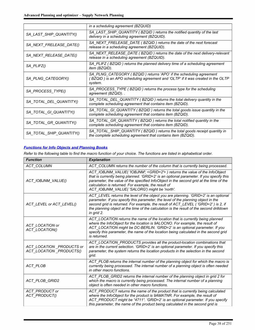
Advanced Planning and optimizer – Supply Network Planning

in a scheduling agreement (BZQUID)

SA_LAST_SHIP_QUANTITY()SA_LAST_SHIP_QUANTITY ( BZQID ) returns the notified quantity of the last delivery in a scheduling agreement (BZQUID).

SA_NEXT_FRELEASE_DATE()SA_NEXT_FRELEASE_DATE ( BZQID ) returns the date of the next forecast release in a scheduling agreement (BZQUID).

SA_NEXT_RELEASE_DATE()SA_NEXT_RELEASE_DATE ( BZQID ) returns the date of the next delivery-relevant release in a scheduling agreement (BZQUID).

SA_PLIFZ()SA_PLIFZ ( BZQID ) returns the planned delivery time of a scheduling agreement item (BZQID).

SA_PLNG_CATEGORY()SA_PLNG_CATEGORY ( BZQID ) returns ‘APO’ if the scheduling agreement ( BZQID ) is an APO scheduling agreement and ‘OLTP’ if it was created in the OLTP system.

SA_PROCESS_TYPE()SA_PROCESS_TYPE ( BZQID ) returns the process type for the scheduling agreement (BZQID). .

SA_TOTAL_DEL_QUANTITY()SA_TOTAL_DEL_QUANTITY ( BZQID ) returns the total delivery quantity in the complete scheduling agreement that contains item (BZQID).

SA_TOTAL_GI_QUANTITY()SA_TOTAL_GI_QUANTITY ( BZQID ) returns the total goods issue quantity in the complete scheduling agreement that contains item (BZQID).

SA_TOTAL_GR_QUANTITY()SA_TOTAL_GR_QUANTITY ( BZQID ) returns the total notified quantity in the complete scheduling agreement that contains item (BZQID).

SA_TOTAL_SHIP_QUANTITY()SA_TOTAL_SHIP_QUANTITY ( BZQID ) returns the total goods receipt quantity in the complete scheduling agreement that contains item (BZQID).

Functions for Info Objects and Planning Books

Refer to the following table to find the macro function of your choice. The functions are listed in alphabetical order.

Function Explanation

ACT_COLUMN ACT_COLUMN returns the number of the column that is currently being processed.

ACT_IOBJNM_VALUE()

ACT_IOBJNM_VALUE( 'IOBJNM'; <GRID=2'> ) returns the value of the InfoObject that is currently being planned. ‘GRID=2’ is an optional parameter. If you specify this parameter, the value of the specified InfoObject in the second grid at the time of the calculation is returned. For example, the result of ACT_IOBJNM_VALUE( 'SALORG') might be 'north'.

ACT_LEVEL or ACT_LEVEL()

ACT_LEVEL returns the level of the object you are planning. ‘GRID=2’ is an optional parameter. If you specify this parameter, the level of the planning object in the second grid is returned. For example, the result of ACT_LEVEL ( 'GRID=2' ) is 2, if the planning object at the time of the calculation is the result of the second drilldown in grid 2.

ACT_LOCATION or ACT_LOCATION()

ACT_LOCATION returns the name of the location that is currently being planned where the InfoObject for the location is 9ALOCNO. For example, the result of ACT_LOCATION might be DC-BERLIN. ‘GRID=2’ is an optional parameter. If you specify this parameter, the name of the location being calculated in the second grid is returned.

ACT_LOCATION _PRODUCTS or ACT_LOCATION _PRODUCTS()

ACT_LOCATION_PRODUCTS provides all the product-location combinations that are in the current selection. ‘GRID=2’ is an optional parameter. If you specify this parameter, the system returns the location products in the selection in the second grid.

ACT_PLOBACT_PLOB returns the internal number of the planning object for which the macro is currently being processed. The internal number of a planning object is often needed in other macro functions.

ACT_PLOB_GRID2ACT_PLOB_GRID2 returns the internal number of the planning object in grid 2 for which the macro is currently being processed. The internal number of a planning object is often needed in other macro functions.

ACT_PRODUCT or ACT_PRODUCT()

ACT_PRODUCT returns the name of the product that is currently being calculated where the InfoObject for the product is 9AMATNR. For example, the result of ACT_PRODUCT might be “4711“. ‘GRID=2’ is an optional parameter. If you specify this parameter, the name of the product being calculated in the second grid is

Page 38 of 251

Advanced Planning and optimizer – Supply Network Planning

Function Explanation

returned.

ACT_RESOURCE or ACT_RESOURCE()

ACT_RESOURCE returns the name of the resource that is currently being planned where the InfoObject name of the resource is 9ARNAME. For example, the result of ACT_RESOURCE might be RES-20_1000_001. ‘GRID=2’ is an optional parameter. If you specify this parameter, the name of the resource being calculated in the second grid is returned.

ACT_USER ACT_USER returns the user name of the current planner.

ACT_VERSION or ACT_VERSION()

ACT_VERSION returns the version that is currently being planned where the InfoObject name of the version is 9AVERSION. 'GRID=2' is an optional argument. If you specify this argument, the version being planned in the second grid is returned.For example, the result of ACT_VERSION( 'GRID=2' ) might be 001.

AGG_LEVEL()

Syntax

AGG_LEVEL('characteristic' [; EXCLUDE_IMP] [GRID=2] )

Characteristic = Technical name of the characteristic that is to be analyzed

EXCLUDE_IMP: If you set this optional indicator ('X'), implicitly strong characteristics are not taken into account in the analysis.

GRID=2: If you set this optional parameter, the analysis is applied to the planning object of the second grid.

Description

The AGG_LEVEL() function analyzes whether the planning object being currently processed is detailed or aggregated with regards to the characteristic characteristic. If detailed, the return value is ‘0’; if aggregated, the value is ‘1’.

The return value of the AGG_LEVEL() function is complementary to the return value of the DET_LEVEL() function.

ALERT_BDATE()

ALERT_BDATE( ALERT ) returns the start date of the earliest valid alert/status of the alert/status type specified by ALERT for the current selection. The argument of this function is an alert/status element. For more information about macro elements, see the Application Help for Demand Planning.

ALERT_EDATE()ALERT_EDATE( ALERT ) returns the finish date of the latest valid alert/status of the alert/status type specified by ALERT for the current selection. The argument of this function is an alert/status element.

ALERT_EXIST()ALERT_EXIST( ALERT ) returns the number of alerts/statuses that exist for alert/status type ALERT for the current selection. The argument of this function is an alert/status element.

ALERT_PROFILE_THRESH()ALERT_PROFILE_THRESH( ‘profile’ ; ‘alert type’ ; ‘alert priority’ ; <’alert object type’> ; <’application’>) returns the threshold value for a particular alert type and priority (information, warning, error) in an alert profile.

ALLOC()

ALLOC( n ; m ; X1 ; ... ; Xn + m + 1 ; Y1 ; ... ; Yn + m + 1 ) returns the open allocation quantity that is available for satisfying sales orders, where n is the number of allocation periods before the current period, m is the number of allocation periods after the current period, Xi is the allocation quantity for period i ( i = 1 ... n + m + 1 ), and Yi is the incoming orders quantity for period i. The arguments can be numbers that you enter in Operator/function dialog boxes as well as rows, columns, cells, or areas from the planning table or auxiliary table.

ALLOC_MISQTY()

ALLOC_MISQTY( n ; m ; X1 ; ... ; Xn + m + 1 ; Y1 ; ... ; Yn + m + 1 ) returns the amount by which the customer has already exhausted their allocation, where n is the number of allocation periods before the current period, m is the number of allocation periods after the current period, Xi is the allocation quantity for period i ( i = 1 ... n + m + 1 ), and Yi is the incoming orders quantity for period i. The arguments can be numbers that you enter in Operator/function dialog boxes as well as rows, columns, cells, or areas from the planning table or auxiliary table.

BUCKET_BDATE()

BUCKET_BDATE( X1 ; ... ; Xn ) returns the earliest start date of the periods given by the cell(s), row(s), and/or column(s) (not areas) X1 through Xn of the planning table or the auxiliary table. This date is expressed in whole numbers with reference to the date 01.01.0001. In the attributes of the argument elements, you must specify Period data as the data source.

Page 39 of 251

Advanced Planning and optimizer – Supply Network Planning

Function Explanation

BUCKET_DATE_IN()

BUCKET_DATE_IN( X ; Y1 ; ... ; Yn ) returns 1 if date X falls within the periods given by the cell(s), row(s), and/or column(s) (not areas) Y1 through Yn. Otherwise, 0 is returned. The date X (for example, the function TODAY or DATE()) is expressed in whole numbers with reference to the date 01.01.0001. The argument can be either a number that you enter in an Operator/function dialog box, or one of the macro elements cell, row, or column from the planning table or the auxiliary table. In the attributes of the argument elements Y1 through Yn, you must specify Period data as the data source.

BUCKET_DAYS()

BUCKET_DAYS( X1 ; ... ; Xn ) returns the number of Gregorian calendar days of the periods given by the cell(s), row(s), and/or column(s) (not areas) X1 through Xn. In the attributes of the argument elements, you must specify Period data as the data source.

BUCKET_DESCRIPTION()BUCKET_DESCRIPTION( X ) returns for the specified column X the text that appears in the column of that period in the planning table.

BUCKET_EDATE()

BUCKET_EDATE( X1 ; ... ; Xn ) returns the latest finish date of the periods given by the cell(s), row(s) and/or column(s) (not areas) X1 through Xn. This date is expressed in whole numbers with reference to the date 01.01.0001. In the attributes of the argument elements, you must specify Period data as the data source.

BUCKET_WDAYS()

BUCKET_WDAYS( <calendar> ; X1 ; ... ; Xn) returns the number of workdays in the periods given by the cell(s), row(s), and/or column(s) (not areas) X1 through Xn. In the attributes of the argument elements, you must specify Period data as the data source. The specification of a calendar as the first argument is optional. If you do not specify a calendar, the system reads the calendar given by the time stream in the storage buckets profile. If no time stream is defined, the system uses calendar days.

CALC_ERRORCALC_ERROR returns the value X if an error has occurred during execution of the macro.

CALENDAR()

CALENDAR( 'location' ; 'calendar type' ; <version> ) returns the calendar of the specified type that is used by the specified location in the specified version. The specification of a version as the third argument is optional. CALENDAR( ACT_LOCATION ; 'PP' ) would return the production planning calendar of the location you are currently planning.

CALENDAR_WDAYS()CALENDAR_WDAYS( ‘calendar’ ; from date ; <to date> ) returns the number of workdays between the from-date and the to-date in the calendar specified.

CBF_DISPLAY_TO_INT()CBF_DISPLAY_TO_INT( row 1 ; …row n ) writes the displayed values in a CBF planning book into the internal memory.

CBF

CBP_SET_INDICATOR()CBP_SET_INDICATOR ('mode') switches the display of the CBP progress indicator on or off. The argument is either 'ON' or 'OFF'. The default value is 'ON'.

CBP_SET_ROUNDING()CBP_SET_ROUNDING ('mode') switches rounding on or off for CBP. The argument is either 'ON' or 'OFF'. The default value is 'ON'.

COLLABORATION()COLLABORATION ( NAME ) returns a value of 1 if you are currently planning collaboration NAME; otherwise, 0. You enter the name NAME of the collaboration as an argument in an Operator/function dialog box.

DELTA_SUM()DELTA_SUM( key figure, drilldown level) runs the DELTA_SUM function for the specified key figure at the specified drilldown level. For more information, see SAP Note 610517. This macro function can only be used at detail level.

DET_LEVEL() Syntax

DET_LEVEL('characteristic' [; EXCLUDE_IMP] [GRID=2] )

Characteristic = Technical name of the characteristic that is to be analyzed

EXCLUDE_IMP: If you set this optional indicator ('X'), implicitly strong characteristics are not taken into account in the analysis.

GRID=2: If you set this optional parameter, the analysis is applied to the planning object of the second grid.

Description

The DET_LEVEL() function analyzes whether the planning object being currently

Page 40 of 251

Advanced Planning and optimizer – Supply Network Planning

Function Explanation

processed is detailed or aggregated with regards to the characteristic characteristic. If detailed, the return value is ‘1’; if aggregated, the value is ‘0’.

Examples

Example 1:

You have selected the products P1 and P2 (characteristic 9AMATNR). DET_LEVEL( '9AMATNR' ) will provide the return value '0' for this planning object because you are at aggregated level with regards to the characteristic 9AMATNR.

Example 2:

The products P1 and P2 are only in location L1 (characteristic 9ALOCNO) due to the characteristics combinations maintained (in DP) or location products (in SNP). You have selected the products P1 and P2 (characteristic 9AMATNR). DET_LEVEL( '9ALOCNO' ) will provide the return value '1' for this planning object because you are at detailed level with regards to the characteristic 9ALOCNO. The 9ALOCNO characteristic is implicitly strong in this case (namely location L1) due to the selection of products P1 and P2 and it is used in the analysis. DET_LEVEL( '9ALOCNO' ; 'X' ) will deliver the return value '0' for this planning object because implicitly strong characteristics are not used for the analysis. A drilldown to the characteristic ‘location’ would characterize it explicitly.

DRILL_DOWN()

DRILL_DOWN( 'characteristic’ , <'internal'>, <’CBF’> ) carries out a drilldown using the specified characteristic (technical name). The display is as for Details (all) in the planning table. If you set the optional argument 'internal,' the display is not changed. This option improves performance if you intend to drill-up in the same macro subsequently.

Set the ‘CBF’ argument if you are working in a CBF planning book and the characteristic is a CBF characteristic. If you want to drill down on a non-CBF characteristic, do not set this argument.

DRILL_IOBJNM()

DRILL_IOBJNM( drill-down level ) returns the technical name of the characteristic that was drilled down on at a particular drill-down level. The drill-down level can be a number 1, 2, and so on or ACT_LEVEL as the current level.

This function is only available if you have drilled down in the grid using the header or by using the DRILL-DOWN macro function.

DRILL_UP()

DRILL_UP( 'characteristic’ , <'internal'>, <’CBF’> carries out a drill-up using the specified characteristic (technical name). If you set the optional argument 'internal,' the display is not changed. This option improves performance if you intend to drill-up in the same macro subsequently.

Set the ‘CBF’ argument if you are working in a CBF planning book and the characteristic is a CBF characteristic. If you want to drill up on a non-CBF characteristic, do not set this argument.

The same rules for drill-down and drill-up apply as in interactive planning.

FIX_CALC()

FIX_CALC( X1; X2: <input check> ) performs fixing calculation with X1 as the row containing the key figure with the value to be fixed and X2 the key figure for the fixed values. If the input check indicator is set (for instance X), the system tries to correct any inconsistencies that may occur due to changes being made on the detail level. For example, a key figure has, at aggregate level, the value 100 and at detail level it has three values (50, 30, and 20). You then change the last value to 40; the system reduces the amounts of the remaining levels so that the total is still 100. Macros that use this function should not be used at detail level.

FORCONS_LOGIC() Syntax

FORCONS_LOGIC( product ; location )

Product: Product ID

Location : Customer location ID

These arguments can be entered using other operators/functions such as ACT_PRODUCT, ACT_LOCATION or as literals in single inverted commas.

Description

FORCONS_LOGIC returns the value 1 if the following conditions are fulfilled:

Page 41 of 251

Advanced Planning and optimizer – Supply Network Planning

Function Explanation

In the customer location, the standard consumption logic has been chosen.

The location product has been assigned a requirements strategy for which the assignment mode is Assign customer requirements to planning with assembly, for example, in the standard requirements strategy 20 – Planning with Final Assembly.

Otherwise, the function returns the value 0.

This function is intended for use with the VMI scenario.

FORECAST_CONSUMPTION()

Syntax

FORECAST_CONSUMPTION( product ; location )

Product: Product ID

Location : Customer location ID

These arguments can be entered using other operators/functions such as ACT_PRODUCT, ACT_LOCATION or as literals in single inverted commas.

Description

FORECAST_CONSUMPTION executes consumption of the VMI forecast by customer requirements for the given customer location and product.

FORECAST_PROFILE_SET()

FORECAST_PROFILE_SET('profile'; 'profile type'; 'version';< key figure 'IOBJNM'> ) sets the forecast profile 'profile' for the forecasting type 'profile type' (S - univariate, M - MLR, C - composite) and the version 'version'. An optional entry is the key figure for which the profile is valid, for example, 9AFCST for the standard forecast key figure.

IOBJNM_VALUE()

IOBJNM_VALUE( 'IOBJNM' ; 'VALUE' ) determines whether the current selection contains only data for the specified characteristic value VALUE of the InfoObject IOBJNM. If yes, the system returns the value 1; otherwise, 0. Enter the arguments in a dialog box of the Operator/function element. Use this function to find out, for example, if the current selection contains data for product VALUE.

INTERNAL_RESOURCE_UNIT()INTERNAL_RESOURCE_UNIT( 'resource' ; 'version' ) returns the unit of measure in which a resource is saved in liveCache.

INVENTORY_COST()

INVENTORY_COST( 'product' ; 'location' ; <'version'> ) returns the inventory cost of the specified product at a specified location in the specified version. The third argument for the version is optional. INVENTORY_COST( ACT_PRODUCT ; ACT_LOCATION ) returns the inventory cost of the currently planned product in the currently planned location.

ITERATION_COUNTERITERATION_COUNTER returns the number of iterations that have been carried out in the current step.

KEYFS_PLOB()KEYFS_PLOB(X) returns the internal number of planning object in row X. In the attributes of the argument row, the value in the Data field must be Row attributes. You can use this function as an argument in other macro functions.

KEYFS_VERSION()KEYFS_VERSION( X ) returns the version of the key figure values in row X. In the attributes of the argument row, the value in the Data field must be Row attributes.

LAYOUTVAR_VALUE()

Syntax

LAYOUTVAR_VALUE( 'my_Variable' )

my_Variable = Name of variables

Description

LAYOUTVAR_VALUE () returns the value of the numeric variables my_Variable. You must assign this value to the variables first with the function LAYOUTVARIABLE_SET ().

LAYOUTVARIABLE() Syntax

LAYOUTVARIABLE( 'my_Variable' )

my_Variable = Name of variables

Description

LAYOUTVARIABLE () returns the character string of the alphanumeric variables my_Variable. You must assign this character string to the variables first with the

Page 42 of 251

Advanced Planning and optimizer – Supply Network Planning

Function Explanation

function LAYOUTVARIABLE_SET ().

LAYOUTVARIABLE_SET()

Syntax

LAYOUTVARIABLE_SET( 'my_Variable' ; value)

my_Variable = Name of variables

Value = numeric value

'Value' = alphanumeric character string

Description

LAYOUTVARIABLE_SET() assigns the numeric value or the alphanumeric character string 'value' to the variable my_Variable . If you want to assign an alphanumeric character string, you set the argument in single inverted commas, that is, 'value'. If you want to assign a numeric value, you use the argument without single inverted commas. You can access the variable my_Variable with the functions LAYOUTVAR_VALUE () and LAYOUTVARIABLE () in other macros of the same planning book. The content of the variables is deleted when new data is loaded into interactive planning. The declaration of the type of variables (numeric or alphanumeric) takes place automatically when setting the variables with LAYOUTVARIABLE_SET ().

LOC()

LOC( 'FIELD_NAME' ; <'location'> ; <'version'> ) returns the content of a numeric field in the location master record of the specified location. The arguments for the location and version are optional. If you do not specify an argument for the location, the system uses the currently planned location. However, it is better for performance reasons to use the ACT_LOCATION function. For example, LOC( 'DURAT' ; ACT_LOCATION ) returns the maximum duration during continuous move of the current location.

LOC_C()

LOC_C( 'FIELD_NAME' ; <'location'> ; <'version'> ) returns the content of a character field in the location master record of the specified location. The arguments for the location and version are optional. If you do not specify an argument for the location, the system uses the currently planned location. However, it is better for performance reasons to use the ACT_LOCATION function. For example, LOC_C( 'PARTNER' ; ACT_LOCATION ) returns the partner for the current location.

LOC_EXTRA()

LOG_EXTRA( n ; <'location'> ; <'version'> ) gets the value of an extra field in the location master record for the specified location in the specified version, where n represents the number of the extra field. For example, LOC_EXTRA( 1 ; ACT_LOCATION ) gets the value in extra field 1 for the currently planned location. The arguments for the location and version are optional. If you do not specify an argument for the location, the system uses the currently planned location. However, it is better for performance reasons to use the ACT_LOCATION function. Use this function for numeric fields.

LOC_EXTRA_C()

LOG_EXTRA_C( n ; <'location'> ; <'version'> ) gets the value of an extra character field in the location master record for the specified location in the specified version, where n represents the number of the extra field. For example, LOC_EXTRA_C( 1 ; ACT_LOCATION ) gets the value in extra field 1 for the currently planned location, if this field is of type character. The arguments for location and version are optional. If you do not specify an argument for the location, the system uses the currently planned location. However, it is better for performance reasons to use the ACT_LOCATION function.

LOC_EXTRA_SET()

LOG_EXTRA_SET( n ; 'field_value' ; <'location'> ; '<version>' ) sets the value of an extra field in the location master record for the specified location in the specified version, where n represents the number of the extra field and 'field_value' represents the character or numerical value you want to give the field. Enter a numerical value without single inverted commas. The arguments for location and version are optional. If you do not specify an argument for the location, the system uses the currently planned location. However, it is better for performance reasons to use the ACT_LOCATION function.

LOC_SET() LOC_SET( ‘field name’ ; 'field_value' ; <'location'> ; '<version>' ) sets the value of the specified field in the location master record for the specified location in the specified version. The arguments for location and version are optional. If you do not specify an argument for the location, the system uses the currently planned location.

Page 43 of 251

Advanced Planning and optimizer – Supply Network Planning

Function Explanation

However, it is better for performance reasons to use the ACT_LOCATION function.

LOCATION_TYPE()LOCATION_TYPE ( 'location' ) returns the location type of the location in the argument, for example ACT_LOCATION.

MAT()

MAT( 'FIELD_NAME' ; <'product'> ; <'version'> ) returns the content of a numerical field in the product master record of the specified product. MAT( 'BRGEW' ; ACT_PRODUCT ) returns the gross weight of the current product. The arguments for product and version are optional. If you do not specify an argument for the product, the system uses the currently planned product. However, it is better for performance reasons to use the ACT_LOCATION function.

MAT_C()

MAT_C( 'FIELD_NAME' ; <'product'> ; <'version'> ) returns the content of a character field in the product master record of the specified product. The arguments for product and version are optional. If you do not specify an argument for the product, the system uses the currently planned product. However, it is better for performance reasons to use the function ACT_PRODUCT. For example, MAT_C( 'KOSCH' ; ACT_PRODUCT ) returns the product allocation procedure for the current product.

MAT_EXTRA()

MAT_EXTRA( n ; <'product'> ; <'version'> ) gets the value of an extra field in the product master record for the specified product in the specified version, where n represents the number of the extra field. The arguments for product and version are optional. If you do not specify an argument for the product, the system uses the currently planned product. However, it is better for performance reasons to use the function ACT_PRODUCT. For example, MAT_EXTRA( 1 ; ACT_PRODUCT ) gets the value in extra field 1 for the currently planned product.

MAT_EXTRA_C()

MAT_EXTRA_C( n ; <'product'> ; <'version'> ) gets the value of an extra character field in the product master record for the specified product in the specified version, where n represents the number of the extra character field. The arguments for product and version are optional. If you do not specify an argument for the product, the system uses the currently planned product. However, it is better for performance reasons to use the function ACT_PRODUCT. For example, MAT_EXTRA( 1 ; ACT_PRODUCT ) gets the value in extra character field 1 for the currently planned product.

MAT_EXTRA_SET()

MAT_EXTRA_SET( n ; 'field_value' ; <'product'> ; '<version>' ) sets the value of an extra field in the product master record for the specified product in the specified version, where n represents the number of the extra field and 'field_value' represents the character or numerical value you want to give the field. Enter a numerical value without single inverted commas. The arguments for product and version are optional. If you do not specify an argument for the product, the system uses the currently planned product. However, it is better for performance reasons to use the function ACT_PRODUCT.

MAT_SET()

MAT_SET ( ‘field name’ ; field_value' ; <'product'> ; '<version>' ) sets the value of the specified field in the product master record for the specified product in the specified version. The arguments for product and version are optional. If you do not specify an argument for the product, the system uses the currently planned product. However, it is better for performance reasons to use the function ACT_PRODUCT.

MATLOC()

MATLOC( 'FIELD_NAME' ; <'product'> ; <'location'> ; <'version'> ) returns the content of a numerical field in the location/product master record of the specified product and location. The arguments for product, location, and version are optional. If you do not specify an argument for the product and/or location, the system uses the current product/location. However, it is better for performance reasons to use the functions ACT_LOCATION and ACT_PRODUCT. For example, MATLOC( 'BSTMA' ; ACT_PRODUCT ; ACT_LOCATION ) returns the maximum lot size for this location product.

MATLOC_C() MATLOC_C( 'FIELD_NAME' ; <'product'> ; <'location'> ; <'version'> ) returns the content of a character field in the location/product master record of the specified product and location. The arguments for product, location, and version are optional. If you do not specify an argument for the product and/or location, the system uses the current product/location. However, it is better for performance reasons to use the functions ACT_LOCATION and ACT_PRODUCT. For example, MATLOC( 'BESKZ' ; ACT_PRODUCT ; ACT_LOCATION ) returns the procurement type for this location

Page 44 of 251

Advanced Planning and optimizer – Supply Network Planning

Function Explanation

product.

MATLOC_EXTRA()

MATLOC_EXTRA( n ; <'product'> ; <'location'> ; <'version'> ) gets the value of an extra field in the product/location master record for the specified product and location in the specified version, where n represents the number of the extra field. The arguments for product, location, and version are optional. If you do not specify an argument for the product and/or location, the system uses the current product/location. However, it is better for performance reasons to use the functions ACT_LOCATION and ACT_PRODUCT. For example, MATLOC_EXTRA( 1 ; ACT_PRODUCT ; ACT_LOCATION ) gets the value in extra field 1 for the currently planned location product. Use this function for numeric fields.

MATLOC_EXTRA_C()

MATLOC_EXTRA( n ; <'product'> ; <'location'> ; <'version'> ) gets the value of an extra character field in the product/location master record for the specified product and location in the specified version, where n represents the number of the extra character field. The arguments for product, location, and version are optional. If you do not specify an argument for the product and/or location, the system uses the current product/location. However, it is better for performance reasons to use the functions ACT_LOCATION and ACT_PRODUCT. For example, MATLOC_EXTRA( 1 ; ACT_PRODUCT ; ACT_LOCATION ) gets the value in extra character field 1 for the currently planned location product.

MATLOC_EXTRA_SET()

MATLOC_EXTRA_SET( n ; 'field_value' ; <'product'> ; <'location'> ; '<version>' ) sets the value of an extra field in the location product master record for the specified product and location in the specified version, where n represents the number of the extra field and 'field_value' represents the character or numerical value you want to give the field. Enter a numerical value without single inverted commas. The arguments for product, location, and version are optional. If you do not specify an argument for the product and/or location, the system uses the current product/location. However, it is better for performance reasons to use the functions ACT_LOCATION and ACT_PRODUCT.

MATLOC_SET()

MATLOC_SET(( ‘field name’ ; ; 'field_value' ; <'product'> ; <'location'> ; '<version>' ) sets the value of the specified field in the location product master record for the specified product and location in the specified version. The arguments for product, location, and version are optional. If you do not specify an argument for the product and/or location, the system uses the current product/location. However, it is better for performance reasons to use the functions ACT_LOCATION and ACT_PRODUCT.

PARTNER()PARTNER( NAME ) returns the value 1 if planning is currently being done by partner NAME; otherwise, 0. You enter the name NAME of the partner as an argument in an Operator/function dialog box. Use this function in Collaborative Planning.

PLOBS_FOR_LEVEL()

PLOBS_FOR_LEVEL( X ) returns the number of planning objects on the specified level where X represents the planning level. For example, PLOBS_FOR_LEVEL( 1 ) returns the number of products in the product group selection if you have first selected a product group and then drilled down to product level.

PRODUCT_LIFE()

PRODUCT_LIFE( X ; <'product'> ) returns the value 1 if data is selected for exactly one product and if the specified date X comes after the phase-in time span and before the phase-out time span of the product. Otherwise, 0 is returned. For example, PRODUCT_LIFE ( DATE ( 20010220 ) ) returns the value 1 if the product is in its growth or maturity phrase on February 20, 2001. The argument can be either a number that you enter in an Operator/function dialog box, or one of the macro elements cell, row, or column from the planning table or the auxiliary table. The argument for product is optional.

PRODUCT_PHIN_END or PRODUCT_PHIN_END()

PRODUCT_PHIN_END( <'GRID=2'> ; <'product'> ) returns the end date of the specified product's launch phase as maintained for the phase-in profile in the product master record. The arguments for grid 2 and product are optional. If you do not specify a product, the system returns the end date of the phase-in time span of the currently planned product. However, for performance reasons, we recommend that you use the function ACT_PRODUCT to represent the current product.

PRODUCT_PHIN_START or PRODUCT_PHIN_START()

PRODUCT_PHIN_START( <'GRID=2'> ; <'product'> ) returns the start date of the specified product's launch phase as maintained for the phase-in profile in the product master record. The arguments for grid 2 and product are optional. If you do not specify a product, the system returns the start date of the phase-in time span of

Page 45 of 251

Advanced Planning and optimizer – Supply Network Planning

Function Explanation

the currently planned product. However, for performance reasons, we recommend that you use the function ACT_PRODUCT to represent the current product.

PRODUCT_PHOUT_END or PRODUCT_PHOUT_END()

PRODUCT_PHOUT_END( <'GRID=2'> ; <'product'> ) returns the end date of the specified product's decline phase as maintained for the phase-out profile in the product master record. The arguments for grid 2 and product are optional. If you do not specify a product, the system returns the end date of the phase-out time span of the currently planned product. However, for performance reasons, we recommend that you use the function ACT_PRODUCT to represent the current product.

PRODUCT_PHOUT_START or PRODUCT_PHOUT_START()

PRODUCT_PHOUT_START( <'GRID=2'> ; <'product'> ) returns the start date of the specified product's decline phase as maintained for the phase-out profile in the product master record. The arguments for grid 2 and product are optional. If you do not specify a product, the system returns the start date of the phase-out time span of the currently planned product. However, for performance reasons, we recommend that you use the function ACT_PRODUCT to represent the current product.

RESOURCE_COST()RESOURCE_COST( 'resource' ; 'resource variant' ; DATE ) returns the cost of the specified resource for the specified capacity variant on the specified date.

RESOURCE_EDIT()RESOURCE_EDIT( 'resource' ; 'version' ) returns the value ' X ' if the resource can be edited in the specified version, ' ' if it cannot.

RESOURCE_OVERLOAD()

RESOURCE_OVERLOAD( 'resource' ; 'version' ) returns the resource overload for the specified resource in the specified version. For example, RESOURCE_OVERLOAD ( ACT_RESOURCE ; ACT_VERSION ) might return 10%.

RESOURCE_RESTYPE()

RESOURCE_RESTYPE( 'resource' ; 'version' ) returns the resource type of the specified resource in the specified version. For example, RESOURCE_RESTYPE( ACT_RESOURCE ; ACT_VERSION ) returns resource type 'P', 'T', 'S,' or 'H' (production, transportation, storage or handling) for the current resource in the current version.

RESOURCE_UNDERLOAD()

RESOURCE_UNDERLOAD( 'resource' ; 'version' ) returns the resource underload for the specified resource in the specified version. For example, RESOURCE_UNDERLOAD ( ACT_RESOURCE ; ACT_VERSION ) might return 10%.

RESOURCE_UNIT()RESOURCE_UNIT ( 'resource' ; 'version' ) returns the unit for the resource that is contained in the resource master record in the specified version.

RESOURCE_VARIANT()RESOURCE_VARIANT( 'version' ; 'resource_variant' ; 'from_date' ; 'to_date' ) returns the available capacity for the specified resource variant in the specified time span.

SUM_CALC()SUM_CALC( key figure ) calculates the sum of all detail levels of the specified key figure.

STDV_DEMAND_GET()

Syntax

STDV_DEMAND_GET([key figure])

Key figure = Enter the name of the combined key figure here (that is, the result key figure).

Description

This function combines the values of one or more forecast key figures to form a single key figure, the combined key figure. The prerequisite for this function is that

you have maintained the master data for demand combination.

STDV_WRITE_ALERTS()

Syntax

STDV_WRITE_ALERTS()

Description

This function generates data base alerts for demand combination, which the Alert Monitor displays. You must call the function STDV_DEMAND_GET() in the same macro before the alerts can be generated.

TIMESHIFT_BACKWARDS()

TIMESHIFT_BACKWARDS( X1 ; ... ; Xn ; Y1 ; ... ; Yn ) shifts the values of time series X1 through Xn backward in time by the number of periods given in time series

Page 46 of 251

Advanced Planning and optimizer – Supply Network Planning

Function Explanation

Y1 through Yn. For example:

The time series look like this: X 10 20 30 40 50Y 1 2 1 3 1. The result looks like this:

30 40 30 - 50 -

The value 10 is shifted back one period in time, the value 20 is shifted back two periods in time, and so on.

TIMESHIFT_FORWARDS()

TIMESHIFT_FORWARDS( X1 ; ... ; Xn ; Y1 ; ... ; Yn ) shifts the values of time series X1 through Xn forward in time by the number of periods given in time series Y1 through Yn. Example: The time series look like this:X 10 20 30 40 50Y 1 3 1 2 1.

The result looks like this: 10 - 30 20 90The value 10 is shifted forward one period in time, the value 20 is shifted forward three periods in time, and so on.

TS_GET()

TS_GET( 'TS_TYPE' ; 'key_value_1' ; 'key_value_2' ; 'key_value_3' ; <value_from> ; <value_to> ) reads the values of a database time series where 'TS_TYPE' defines the time series type, the second, third and fourth arguments represent the values from the three possible key fields of the time series, and the fifth and sixth arguments (which are optional) define the value range that you want to read.

The mandatory fields have the following types:

TSTYPE = CHAR 20key_value1 = CHAR 60key_value2 = CHAR 60key_value3 = CHAR 60

Example: A time series with ID 'I'', 'A'; 'B'; 'C' is

Item 1 2 3 4 5 6 7 8 9Value 10 10 20 30 50 50 60 90 120.

TSGET ( ''I'', 'A' ; 'B' ; 'C' ; 2 ; 9 ) returns10 20 30 50 50 60 90 120

Use an area as the macro result element.

TS_SET()

TS_SET( 'TS_TYPE' ; 'key_value_1' ; 'key_value_2' ; 'key_value_3' ; from_value ; Y1 ; ... ; Yn ) writes values to a database time series where 'TS_TYPE' defines the time series type, the second, third and fourth arguments represent the values from the three possible key fields of the time series. These fields are defined for TS_GET(). The fifth argument specifies at which bucket the system should start to write the data (for example, 5 = start at bucket 5). The value of this argument must be a whole number ≥ 1. Y1 through Yn are the values to be written. These values can be numbers or other functions that define these values.

VALUE_CONTAINED()VALUE_CONTAINED( value ; range ) returns the value 1 if the value is contained in the specified range.

VEC_LAYOUTVARIABLE() Syntax

VEC_LAYOUTVARIABLE( 'my_vector' [; from_index [; to_index ] ] )

my_vector = Name of vector

from_index = Index that specifies the start of the interval to be read

to_index = Index that specifies the end of the interval to be read

Description

The contents of the vector my_vector are assigned to a results area (tableau element area). Optionally, you can specify an index from_index so that the contents of the vector my_vector are assigned as of the index from_index. If you have specified an index from_index, you can also specify the index to_index so

Page 47 of 251

Advanced Planning and optimizer – Supply Network Planning

Function Explanation

that the contents of the vector are only assigned to the results area up to the index to_index.

VEC_LAYOUTVARIABLE_SET()

Syntax

VEC_LAYOUTVARIABLE_SET ( ‘my_vector’ ; table_element )

my_vector = Name of vector variable

table_element = Row, column, cell, or area

Description

VEC_LAYOUTVARIABLE_SET() assigns the numerical values in table_element to the vector variable my_vector.

VEC_LAYOUTVARIABLE_APP()

Syntax

VEC_LAYOUTVARIABLE_APP ( ‘my_vector’ ; table_element )

my_vector = Name of vector variable

table_element = Row, column, cell, or area

Description

VEC_LAYOUTVARIABLE_APP() assigns the values in table_element to the vector variable my_vector.

W_AVG_CALC()W_AVG_CALC (key figure with values; key figure with weighting factors) calculates the weighted average of the first key figure using the weighting factors given in the second key figure.

Multilevel Functions in the Supply Chain Network

These four functions enable you to determine statistical values for use with multilevel scenarios.

In the above graphic example, the figures represent the planned consumption of a product at different levels in the supply chain for one particular period. As well as aggregating the demand from the lower levels the locations also have their own consumption.

The function MULTILEVEL_DEMAND_MEAN forms the sum of these planned demands, in this case 100 + 150 + 130 + 40 + 20 = 440.

The function MULTILEVEL_DEMAND_VAR determines the error variance between the planned and actual values for the whole specified period or if you have not specified a period, the complete past.

(Error variance = where and are the planned and actual values respectively.)

Page 48 of 251

Advanced Planning and optimizer – Supply Network Planning

The function MULTILEVEL_LEAD_MEAN calculates the planned lead-time for a customer to a receive a product in the period. The system always uses the longest lead-time that is the values from the critical path. The system considers the time from the customer back to the next location that has safety stock. In the above graphic the value would be 6 days.

The function MULTILEVEL_LEAD_VAR determines the error variance between the planned and actual values for the whole specified period or if you have not specified a period, the complete past.

(Error variance = where and are the planned and actual values respectively.)

Date Functions

Refer to the following table to find the function of your choice. The functions are listed in alphabetical order.

Function Explanation

ALERT_BDATE()ALERT_BDATE( ALERT ) returns the start date of the earliest valid alert/status of the alert/status type specified by ALERT for the current selection. The argument of this function is an alert/status element.

ALERT_EDATE()ALERT_EDATE( ALERT ) returns the finish date of the latest valid alert/status of the alert/status type specified by ALERT for the current selection. The argument of this function is an alert/status element.

BUCKET_BDATE()

BUCKET_BDATE( X1 ; ... ; Xn ) returns the earliest start date of the periods given by the cell(s), row(s), and/or column(s) (not areas) X1 through Xn of the planning table or the auxiliary table. This date is expressed in whole numbers with reference to the date 0001/01/01. In the attributes of the argument elements, you must specify Period data as the data source.

BUCKET_DATE_IN()

BUCKET_DATE_IN( X ; Y1 ; ... ; Yn ) returns 1 if date X falls within the periods given by the cell(s), row(s), and/or column(s) (not areas) Y1 through Yn. Otherwise, 0 is returned. The date X (for example, the function TODAY or DATE()) is expressed in whole numbers with reference to the date 0001/01/01. The argument can be either a number that you enter in an Operator/function dialog box, or one of the macro elements cell, row, or column from the planning table or the auxiliary table. In the attributes of the argument elements Y1 through Yn, you must specify Period data as the data source.

BUCKET_DAYS()BUCKET_DAYS( X1 ; ... ; Xn ) returns the number of Gregorian calendar days of the periods given by the cell(s), row(s), and/or column(s) (not areas) X1 through Xn. In the attributes of the argument elements, you must specify Period data as the data source.

BUCKET_EDATE()

BUCKET_EDATE( X1 ; ... ; Xn ) returns the latest finish date of the periods given by the cell(s), row(s) and/or column(s) (not areas) X1 through Xn. This date is expressed in whole numbers with reference to the date 0001/01/01. In the attributes of the argument elements, you must specify Period data as the data source.

BUCKET_FISCAL_PERIOD() see FISCAL_PERIOD()

BUCKET_WDAYS() BUCKET_WDAYS( <calendar> ; X1 ; ... ; Xn) returns the number of workdays in the periods given by the cell(s), row(s), and/or column(s) (not areas) X1 through Xn. In the attributes of the argument elements, you must specify Period data as the data source. The specification of a calendar as the first argument is optional. If you do not specify a calendar, the system reads the calendar given by the time stream in the storage buckets

Page 49 of 251

Advanced Planning and optimizer – Supply Network Planning

Function Explanation

profile. If no time stream is defined, the system uses calendar days.

CALENDAR_WDAYS()CALENDAR_WDAYS (‘calendar’; from date; <to date> ) returns the number of workdays between the from-date and the to-date in the calendar specified. The calendar is the timestream ID.

DATE()

DATE (YYYYMMDD ) returns the integer value which corresponds to the number of days between 0001/01/01 and the specified date. You enter the date YYYYMMDD in the format YYYYMMDD in an Operator/function dialog box. For example, DATE (19990101) = 729756. Use this function in order to include a fixed, known date in a macro.

DATE_TO_CHAR ()

Syntax

DATE_TO_CHAR (Number of days)

Number of days: Number of days since 0001/01/01.

Description

DATE_TO_CHAR () returns the date as a string. The function calculates the date starting at 0001/01/01 and adding the Number of days. The system uses the date format that is saved in user master data.

DAY()

DAY( X ) returns the day in a date that is expressed in whole numbers with reference to the date 0001/01/01. Example: DAY( DATE( 19990220)) = 20. The argument can either be a number you enter in an Operator/Function dialog box or one of the macro elements cell, row, or column from the planning table or auxiliary table.

FISCAL_BDATE()

FISCAL_BDATE( X, 'fiscal year variant' ) returns the start of the posting period that contains the date X (expressed in whole numbers with reference to the date 0001/01/01). You can enter the date as DATE ( 19990101 ) or use other date functions such as BUCKET_EDATE(). The second argument specifies the fiscal year variant.

FISCAL_EDATE()

FISCAL_EDATE( X, 'fiscal year variant' ) returns the end of the posting period that contains the date X (expressed in whole numbers with reference to the date 0001/01/01). You can enter the date as DATE ( 19990101 ) or use other date functions such as BUCKET_EDATE(). The second argument specifies the fiscal year variant.

FISCAL_PERIOD() FISCAL_PERIOD(X) returns the number of the posting period specified by column X.

FISCAL_YEAR FISCAL_YEAR (X) returns the fiscal year of the period specified by column X.

MONTH()

MONTH( X ) returns the month in a date that is expressed in whole numbers with reference to the date 01/01/0001. Example: MONTH( DATE( 19990220 )) = 2. The argument can either be a number you enter in an Operator/Function dialog box or one of the macro elements cell, row, or column from the planning table or auxiliary table.

MONTH_BDATE()MONTH_BDATE( X ) returns the start date of the month given in the argument in integer format with reference to the date 0001/01/01.

MONTH_EDATE()MONTH_EDATE( X ) returns the finish date of the month given in the argument in integer format with reference to the date 0001/01/01.

PRODUCT_PHIN_END or PRODUCT_PHIN_END()

PRODUCT_PHIN_END( <'GRID=2'> ; <'product'> ) returns the end date of the specified product's launch phase as maintained for the phase-in profile in the product master record. The arguments for grid 2 and product are optional. If you do not specify a product, the system returns the end date of the phase-in time span of the currently planned product. However, for performance reasons, we recommend that you use the function ACT_PRODUCT to represent the current product.

PRODUCT_PHIN_START or PRODUCT_PHIN_START()

PRODUCT_PHIN_START( <'GRID=2'> ; <'product'> ) returns the start date of the specified product's launch phase as maintained for the phase-in profile in the product master record. The arguments for grid 2 and product are optional. If you do not specify a product, the system returns the start date of the phase-in time span of the currently planned product. However, for performance reasons, we recommend that you use the function ACT_PRODUCT to represent the current product.

PRODUCT_PHOUT_END or PRODUCT_PHOUT_END()

PRODUCT_PHOUT_END( <'GRID=2'> ; <'product'> ) returns the end date of the specified product's decline phase as maintained for the phase-out profile in the product master record. The arguments for grid 2 and product are optional. If you do not specify a product, the system returns the end date of the phase-out time span of the currently planned product. However, for performance reasons, we recommend that you use the

Page 50 of 251

Advanced Planning and optimizer – Supply Network Planning

Function Explanation

function ACT_PRODUCT to represent the current product.

PRODUCT_PHOUT_START or PRODUCT_PHOUT_START()

PRODUCT_PHOUT_START( <'GRID=2'> ; <'product'> ) returns the start date of the specified product's decline phase as maintained for the phase-out profile in the product master record. The arguments for grid 2 and product are optional. If you do not specify a product, the system returns the start date of the phase-out time span of the currently planned product. However, for performance reasons, we recommend that you use the function ACT_PRODUCT to represent the current product.

QUARTER()

Syntax

QUARTER ( Number of days )

Number of days: Number of days since 0001/01/01.

Description

QUARTER() returns the quarter (as a number 1 to 4) in which the date, expressed as the number of days since 0001/01/01, lies. You can convert a date in the normal format to the number of days format by using functions DATE or TODAY.

QUARTER_BDATE()

Syntax

QUARTER_BDATE ( Number of days )

Number of days: Number of days since 0001/01/01.

Description

QUARTER_BDATE() returns the first date of the quarter in which the date, expressed as the number of days since 0001/01/01, lies. You can convert a date in the normal format to the number of days format by using functions DATE or TODAY.

QUARTER_EDATE()

Syntax

QUARTER_EDATE ( Number of days )

Number of days: Number of days since 0001/01/01.

Description

QUARTER_EDATE() returns the last date of the quarter in which the date, expressed as the number of days since 0001/01/01, lies. You can convert a date in the normal format to the number of days format by using functions DATE or TODAY.

SEASON_BDATE

Syntax

SEASON_BDATE ( Column )

Column: Row, column, or cell element (data source = column attributes)

Description

The SEASON_BDATE function determines the start date of a season if all the characteristic values combinations selected for the planning object have the same start date.

SEASON_EDATE

Syntax

SEASON_EDATE ( Column )

Column: Row, column, or cell element (data source = column attributes)

Description

The SEASON_EDATE function determines the end date of a season if all the characteristic values combinations selected for the planning object have the same end date.

TIMESHIFT_BACKWARDS() Syntax

TIMESHIFT_BACKWARDS( <’E’;> Area 1 ; Area 2 )

'E': optional parameter for controlling the behavior at the end of the period

Area 1: Name of the area that contains the data to be moved

Area 2:Name of the area that contains the offsets

The two areas should have the same length and consist of only one line.

Description

TIMESHIFT_BACKWARDS() moves the values of the time series in area 1 back by the

Page 51 of 251

Advanced Planning and optimizer – Supply Network Planning

Function Explanation

number of periods specified in area 2. If you set the optional parameter 'E', values that are moved back beyond the first period in area 1, are either lost or are added to the first period.

For example:

the time series look like this:

Area 1 10 20 30 40 50

Area 2 1 2 1 3 1.

The result looks like this if parameter E was set:

Results 40 30 0 50 0

If E is not set, the result is as follows:

Result 70 30 0 50 0

TIMESHIFT_FORWARDS()

Syntax

TIMESHIFT_ FORWARDS ( <’E’;> Area 1 ; Area 2 )

'E': optional parameter for controlling the behavior at the end of the period

Area 1: Name of the area that contains the data to be moved

Area 2:Name of the area that contains the offsets

The two areas should have the same length and consist of only one line.

Description

TIMESHIFT_FORWARDS() moves the values of the time series in area 1 forward by the number of periods specified in area 2. If you set the optional parameter 'E', values that are moved forward beyond the last period in area 1, are either lost or are added to the last period.

TODAY

TODAY returns today's date in integer format with reference to the date 0001/01/01. For example, you can use this function as the argument of another function:

DAY ( TODAY )

WEEK ( TODAY )

MONTH ( TODAY )

PRODUCT_LIFE ( TODAY )

WEEKDAY ( TODAY )

WEEK_BDATE( TODAY )

WEEK_EDATE( TODAY )

YEAR ( TODAY )

YEAR_BDATE( TODAY )

YEAR_EDATE( TODAY )

BUCKET_DATE_IN ( TODAY ; ... )

WEEK()

WEEK( X ) returns the week in a date X that is expressed in whole numbers with reference to the date 0001/01/01. Example: WEEK( DATE( 20001220)) = 51. The argument can either be a number you enter in an Operator/Function dialog box or one of the macro elements cell, row, or column from the planning table or auxiliary table.

WEEK_BDATE()WEEK_BDATE( X ) returns the start date of the week in which the specified day X falls. For example, if today's date is Wednesday, December 20th in the year 2000, WEEK_BDATE( TODAY ) returns 20001218.

WEEK_EDATE()WEEK_EDATE( X ) returns the end date of the week in which the specified day X falls. For example, if today's date is Wednesday, December 20th in the year 2000, WEEK_EDATE( TODAY ) returns 20001224.

YEAR_BDATE()YEAR_BDATE( X ) returns the start date of the year in which the specified day X falls. For example, if today's date is Wednesday, December 20th in the year 2000, YEAR_BDATE( TODAY ) returns 20000101.

YEAR_EDATE() YEAR_EDATE( X ) returns the end date of the year in which the specified day X falls. For example, if today's date is Wednesday, December 20th in the year 2000, YEAR_EDATE(

Page 52 of 251

Advanced Planning and optimizer – Supply Network Planning

Function Explanation

TODAY ) returns 20001231.

WEEKDAY()

WEEKDAY( X ) returns as a number between 1 and 7 the weekday of a date that is expressed in integer format with reference to the date 0001/01/01, where 1 = Monday and 7 = Sunday. For example, for January 20th 1999 WEEKDAY( DATE( 19990120 ) ) returns 3. The argument can be either a number that you enter in an Operator/function dialog box, or one of the macro elements cell, row or column from the planning table or the auxiliary table.

YEAR()

YEAR( X ) returns the year of a date that is in whole numbers with reference to the date 0001/01/01. Example: For January 20th 1999 YEAR( DATE( 19990120 ) ) returns 1999. The argument can be either a number that you enter in an Operator/function dialog box, or one of the macro elements cell, row or column from the planning table or the auxiliary table.

General and Planning Table Functions

Refer to the following table to find the macro function of your choice. The functions are listed in alphabetical order.

Function Explanation

CELL_BG()

Syntax

CELL_BG( Color [; ToolTip] )

Color: Whole number color code between 0 and 64

ToolTip: String displayed as a ToolTip of the cell (optional)

Description

CELL_BG sets the background color of a cell.

CELL_FG()

Syntax

CELL_FG( Color [; ToolTip] )

Color: Whole number color code between 0 and 64

ToolTip: String displayed as a ToolTip of the cell (optional)

Description

CELL_FG sets the foreground color of a cell.

CELL_INPUT()

Syntax

CELL_INPUT( Read_only_mode )

Read_only_mode: Whole number value 0, 1, or 2

Description

The CELL_INPUT function sets the ready for input status of a cell. The Read_only_mode parameter determines the status. The value 0 sets the cell's status to Not ready for input. The value 1 sets the cell's status to Ready for input. The value 2 determines that the cell adapts the status of the corresponding row. If no status has been set for the row, the value 2 determines that the cell adapts the status of the corresponding column.

CELL_LICON()

Syntax

CELL_LICON( Icon [; ToolTip] )

Icon: Whole number icon code between 0 and 29

ToolTip: String displayed as a ToolTip of the icon (optional)

Description

CELL_LICON sets an icon left-aligned in a cell.

CELL_RICON()

Syntax

CELL_RICON( Icon [; ToolTip] )

Icon: Whole number icon code between 0 and 29

ToolTip: String displayed as a ToolTip of the icon (optional)

Description

CELL_RICON sets an icon right-aligned in a cell.

Page 53 of 251

Advanced Planning and optimizer – Supply Network Planning

Function Explanation

CELL_TOOLTIP()

Syntax

CELL_TOOLTIP( ToolTip )

ToolTip: String displayed as a ToolTip of the cell

Description

CELL_TOOLTIP sets a ToolTip for a cell. The ToolTip can be entered directly as a string or can be determined using the macro function GET_TEXT (language-dependent), for example.

CHAR_VALUES_INPUT()

CHAR_VALUES_INPUT ( 'dialog_box_description' ; 'field_label_1' ; ... ; 'field_label_n' ) prompts the user to enter n character strings in a dialog box that appears automatically when this function is executed. A maximum of 10 character strings can be entered. Thus, you can have a maximum of 11 arguments for this function. As the first argument you specify the text that will appear in the title bar of the dialog box. Write this text in single inverted commas with underscores between each word. As the other arguments, you specify the field labels for the fields in which the user will enter the character strings.

COL_BG()

Syntax

COL_BG( Color [; ToolTip] )

Color: Whole number color code between 0 and 64, 100 and 164, or 200 and 264.

ToolTip: String displayed as a ToolTip of the column (optional)

Description

COL_BG sets the background color of a column.

COL_FG()

Syntax

COL_FG( Color [; ToolTip] )

Color: Whole number color code between 0 and 64, 100 and 164, or 200 and 264.

ToolTip: String displayed as a ToolTip of the column (optional)

Description

COL_FG sets the foreground color of a column.

COL_INPUT()

COL_INPUT( X ) sets the input status of a column. If X = 1, the status of the column is ready for input. If X = 0, the status of the column is read-only. The argument can be either a number that you enter in an Operator/function dialog box, or one of the macro elements cell, row, or column from the planning table or the auxiliary table. You can apply this function to a column or cell of the planning table. In the attributes of the column or cell, set the Scope of change to Attributes. This applies to Grid 1. To refer to Grid 2 use X = 20 for read-only, and X = 21 for ready for input. Similarly X = 10 and X = 11 to refer just to GRID 1.

COL_LICON()

Syntax

COL_LICON( Icon [; ToolTip] )

Icon: Whole number icon code between 0 and 29

ToolTip: String displayed as a ToolTip of the icon (optional)

Description

COL_LICON sets an icon left-aligned in a column.

COL_RICON()

Syntax

COL_RICON( Icon [; ToolTip] )

Icon: Whole number icon code between 0 and 29

ToolTip: String displayed as a ToolTip of the icon (optional)

Description

COL_RICON sets an icon right-aligned in a column.

COL_TOOLTIP() Syntax

COL_TOOLTIP( ToolTip )

ToolTip: String displayed as a ToolTip of the column.

Description

COL_TOOLTIP sets a ToolTip for a column. The ToolTip can be entered directly as a string or can be determined using the macro function GET_TEXT (language-dependent), for

Page 54 of 251

Advanced Planning and optimizer – Supply Network Planning

Function Explanation

example.

COL_VISIBLE()

COL_VISIBLE( X ) sets the visibility of a column. If X = 1, the column is visible. If X = 0, the column is not visible. The argument can be either a number that you enter in an Operator/function dialog box, or one of the macro elements cell, row, or column from the planning table or the auxiliary table. You can apply this function to a column or cell of the planning table. In the attributes of the column or cell, set the Data source to Attributes. This applies to Grid 1. To refer to Grid 2 use X = 20 for read-only, and X = 21 for ready for input. Similarly X = 10 and X = 11 to refer just to GRID 1.

COLUMN_FROM

Syntax

COLUMN_FROM

Description

The COLUMN_FROM function provides the index of the first column of a macro step interval (compare ACT_COLUMN and COLUMN_TO).

COLUMN_MARKED()COLUMN_MARKED returns the value 1 if the column specified in the argument has been selected. Otherwise the value is 0. In the attributes of the row or cell, set the Data source to Row Attributes.

COLUMN_TO

Syntax

COLUMN_TO

Description

The COLUMN_TO function provides the index of the last column of a macro step interval (compare ACT_COLUMN and COLUMN_FROM).

CURR_CONV_FAC()

CURR_CONV_FAC( 'source currency' ; 'target currency' ; 'exchange rate type' ; DATE ) returns the currency conversion factor for the specified source currency, target currency and exchange rate type on the specified date. This date can be TODAY (that is, the system date) or another (see the functions DATE() and TODAY). TODAY is a function, so you do not need to put it in inverted commas. Example: CURR_CONV_FAC( 'USD' ; 'EUR' ; 'M' ; TODAY ).

DATA_IS_LOCKEDDATA_IS_LOCKED returns the value 1, if the data is locked for the current user, meaning they can edit the data. It returns the value 0, if the data is locked by another user, meaning the current user cannot edit the data.

DISPLAY_CONV_FACTOR()

DISPLAY_CONV_FACTOR (Row) returns the conversion factor between the unit in which the data is stored internally and the unit in which it is displayed for the row. For example, time data may be stored in LiveCache in seconds but it is displayed in the planning table in hours. DISPLAY_CONV_FACTOR would then return 3600 In the attributes of the row or cell, set the Data source to Row Attributes.

EVAL()

EVAL() is an auxiliary function for constructing more complicated functions. EVAL() evaluates the arithmetic expression in the argument so that this result can be used in another function. The argument can be either a number that you enter in an Operator/function dialog box, or one of the macro elements cell, row, or column from the planning table or the auxiliary table.

Use this function to calculate the argument of other functions at runtime.

For example EVAL ( ( 1 + 2 ) * 3 ) = 9

GET_TEXT() Syntax

GET_TEXT( TextID [; Language] )

TextID: Text ID for identifying the text element to be read.

Language: Parameter for specifying the language (optional)

Description

GET_TEXT returns the language-dependent text of the text element TextID. The text element TextID must exist as a macro text in at least one language.

If you do not specify the language parameter, the text element is read in the logon language. If the text element is not available in the logon language, it is returned in English or in whatever language is available.

If you specify the language parameter, the system first looks for the text element in that language. If the text element is not available in this language, it is returned in English or in

Page 55 of 251

Advanced Planning and optimizer – Supply Network Planning

Function Explanation

whatever language is available.

HELPTAB_CLEARHELPTAB_CLEAR initializes the values in the auxiliary table. You can use this function anywhere in a macro. If you wish to initialize the values in the auxiliary table at the beginning of a macro, leave unchecked the macro attribute Do not initialize auxiliary table.

IS_FIXED()

Syntax

IS_FIXED( Key Figure )

Key Figure: Row, column, or cell element (data source = row attributes)

Description

The IS_FIXED function returns the value 1 if the cell is completely fixed. (The column results from the current step iteration; the row is determined by the Key Figure parameter.) If the cell is not fixed or partially fixed, the return value is 0. The function is not available if the compatibility mode is activated for the macro book.

IS_INITIAL()

Syntax

IS_INITIAL( Key Figure )

Key Figure: Row, column, or cell element (data source = row attributes)

Description

The IS_INITIAL function returns the value 1 if the cell is initial. (The column results from the current step iteration; the row is determined by the Key Figure parameter.) Apply this function for key figures that can distinguish between zero values and initial values. This function is not available if the compatibility mode is activated for the macro book.

IS_PARTLY_FIXED()

Syntax

IS_PARTLY_FIXED( Key Figure )

Key Figure: Row, column, or cell element (data source = row attributes)

Description

The IS_PARTLY_FIXED function returns the value 1 if the cell is partially fixed. (The column results from the current step iteration; the row is determined by the Key Figure parameter.) If the cell is not fixed or is completely fixed, the return value is 0. The function is not available if the compatibility mode is activated for the macro book.

MARKED_COLUMN() or

MARKED_COLUMN

MARKED_COLUMN(<'FIRST/LAST'>) returns the column numbers of all marked columns. If 'FIRST' or 'LAST' is included as an argument, the function returns the first or last marked column in the time series. 'FIRST' and 'LAST' are the only possible arguments.

MARKED_PLOBMARKED_PLOB returns the internal planning object number of the marked rows. Using this number has the advantage in comparison to the row number that this number remains constant irrespective of where the object appears in the grid.

MARKED_ROW() orMARKED_ROW

MARKED_ROW(<'FIRST/LAST'>) returns the row numbers of all marked rows. If 'FIRST' or 'LAST' is included as an argument, the function returns the first or last marked row. 'FIRST' and 'LAST' are the only possible arguments.

NUM_VALUES_INPUT()

NUM_VALUES_INPUT ( 'dialog_box_description' ; 'field_label_1' ; ... ; 'field_label_n' ) prompts the user to enter n numerical values in a dialog box that appears automatically when this function is executed. As the first argument you specify the text that will appear in the title bar of the dialog box. Write this text in single inverted commas with underscores between each word or use the function STRING_CONCATENATE () . As the other arguments, you specify the field labels for the fields in which the user will enter the numerical values. A maximum of 10 numerical values can be entered. Thus, you can have a maximum of 11 arguments for this function.

NUMBER()

NUMBER( E1 ; ... ; En ) returns the total number of cells in the macro elements E1 through En. E1 through En can be cell(s), row(s), column(s) and/or area(s) from either the planning table or the auxiliary table.For instance, you can use this function to determine the number of time buckets in the current grid.

OUTPUT_POPUP

OUTPUT_POPUP('dialog_box_description' ; 'field_label_1' ; value in field 1 ; ... ; 'field_label_10' ; value in field 10 ) opens a dialog box that shows the alphanumeric or numerical values of extra fields in the product and/or location master record. A maximum of 10 field values can be displayed in this box.

Page 56 of 251

Advanced Planning and optimizer – Supply Network Planning

Function Explanation

PLOB_DATA_VISIBLE()

PLOB_DATA_VISIBLE( X; 'planning object'...'planning object n' ) sets the visibility of the specified planning object(s). You use this function if you are working with drill-down in the Details (all) view. If X =1 the planning objects are displayed. If X=0 the planning objects are hidden. Use functions ACT_PLOB, MARKED_PLOB, or KEYFS_PLOB to specify the planning objects.

PLOB_MARKED()PLOB_MARKED returns the value 1 if the planning object specified in the argument has been selected. Otherwise the value is 0. Use functions ACT_PLOB, MARKED_PLOB, or KEYFS_PLOB to specify the planning objects.

REPORT_SUBMIT()

REPORT_SUBMIT( 'program_name' ; <'job_name'> ; <'job_number'>; <'newmode'>) causes the specified program to be executed. Use the optional arguments, job name and job number, if you wish the program to run in the background. If you set the argument 'newmode', the results are displayed in a new window.

ROW_BG()

Syntax

ROW_BG( Color [; ToolTip] )

Color: Whole number color code between 0 and 64

ToolTip: String displayed as a ToolTip of the row (optional)

Description

The function ROW_BG set the background color of a row.

ROW_CLEAR()

Syntax

ROW_CLEAR( key figure)

Key figure: Rows of the key figure of the planning area. You can enter the key figure two ways:

● As the internal number of the key figure. This is the position of the key figure in the table on the Key Figure tab page of planning area maintenance

● By including the row as the argument. In this case you must the data source to Row Attributes in the Macro Workbench

Description

ROW_CLEAR() deletes all values of the key figure at aggregate (total) level. The value 0 is then disaggregated to all detail levels. Thus it is sufficient to execute the macro only at aggregate level. Similarly it is sufficient to include the function in a step with only one iteration.

ROW_FG()

Syntax

ROW_FG( Color [; ToolTip] )

Color: Whole number color code between 0 and 64

ToolTip: String displayed as a ToolTip of the row (optional)

Description

The function ROW_FG set the foreground color of a row.

ROW_INPUT()

ROW_INPUT( X ) sets the input status of a row. If X = 1, the status of the cell is set to ready-for-input. If X = 0, the status of the cell is set to read-only. The argument can be either a number that you enter in an Operator/function dialog box, or one of the macro elements cell, row, or column from the planning table or the auxiliary table. You can apply this function to a row or cell. In the attributes of the row or cell, set the Scope of change to Attributes.

Note: It is not possible to use this function in conjunction with key figure-specific locking and

the Do not lock read-only key figures option. For more information, see Key Figure Specific Locking.

ROW_LICON() Syntax

ROW_LICON( Icon [; ToolTip] )

Icon: Whole number icon code between 0 and 29

ToolTip: String displayed as a ToolTip of the icon (optional)

Page 57 of 251

Advanced Planning and optimizer – Supply Network Planning

Function Explanation

Description

The function ROW_LICON sets an icon left-aligned in a row.

ROW_MARKED()ROW_MARKED returns the value 1 if the row specified in the argument has been selected. Otherwise the value is 0.

ROW_RICON()

Syntax

ROW_RICON( Icon [; ToolTip] )

Icon: Whole number icon code between 0 and 29

ToolTip: String displayed as a ToolTip of the icon (optional)

Description

The function ROW_RICON sets an icon right-aligned in a row.

ROW_TOOLTIP()

Syntax

ROW_TOOLTIP( ToolTip )

ToolTip: String displayed as a ToolTip of the row

Description

The function ROW_TOOLTIP sets a ToolTip for a row.

ROW_VALUES_CHANGED()

ROW_VALUES_CHANGED( X ) returns 1 if the user has changed one or more values in row X in the current planning session since last pressing Enter. In the attributes of the row, enter Row Attributes as the data source. Note: Since you generally choose Enter when entering values, SAP recommends that you use macros with this functions as default macros.

ROW_VISIBLE()

ROW_VISIBLE( X ) sets the visibility of a row. If X = 1, the row is visible. If X = 0, the row is not visible. The argument can be either a number that you enter in an Operator/function dialog box, or one of the macro elements cell, row, or column from the planning table or the auxiliary table. You can apply this function to a row or cell. In the attributes of the row or cell, set the Scope of change to Attributes.

STEP_AREA_SET()

Syntax

STEP_AREA_SET( From-Column ; To-Column )

From-column: Column index

To-column: Column index

Description

The STEP_AREA_SET function sets the step interval of all the following macro steps to from-column to to-column. This way, the macro step interval that you defined in the MacroBuilder is overridden. However, the step interval of the macro step in which the STEP_AREA_SET function is called is not changed.

The step interval set by the STEP_AREA_SET function is valid until the end of the macro execution or can be cancelled by calling STEP_AREA_SET( 0 ; 0 ).

STEP_CALC_STOP

Syntax

STEP_CALC_STOP

Description

The STEP_CALC_STOP function leaves a macro step after carrying out the current step iteration. Any assignments and macro functions that exist after calling STEP_CALC_STOP will still be executed.

STRINGS_CONCATENATE()

STRINGS_CONCATENATE('string1'...'stringn') inserts blanks between several character strings to produce one string.

UNIT_CONV_FAC()UNIT_CONV_FAC( NAME1 ; NAME2 ) returns the conversion factor for conversion from unit NAME1 to unit NAME2. You enter the names of the units in Operator/function dialog boxes; for example, UNIT_CONV_FAC ( KG ; TO ) = 1000.

USER()USER( NAME ) = 1 if the user name of the person who logged on is NAME; for example, USER( SUCHANEK ) = 1 if the logon name of the planner is Suchanek. Otherwise, USER( SUCHANEK ) = 0. You enter the argument in an Operator/function dialog box.

VALUE_OF_ROW_CHAN VALUE_OF_ROW_CHANGED( X ; Y1 ; ... Yn ) returns 1 if the user has changed one or

Page 58 of 251

Advanced Planning and optimizer – Supply Network Planning

Function Explanation

GED()more key figure values in columns Y1 through Yn of row X in the current planning session since last pressing Enter. In the attributes of the row, enter Row Attributes as the data source.

Attributes of Macro Elements

You can change the attributes of the various macro elements (macros, steps, conditions, and so on). The attributes that can be edited vary with the element type and include the periods for which the element is valid and additional functions.

Features

For each macro element, you can change the name in the attributes.

Macro

Here you specify:

Whether the macro can be executed directly

Whether a confirmation prompt appears when you execute the macro

Whether the auxiliary table is initialized when you call the macro

If the auxiliary table is not initialized when you call the macro, any values that are in the table from the execution of previous macros remain in the table and can be used in the current macro. All entries in the auxiliary table are lost when you leave the planning book.

Which change mode is to be performed, for example, a value change or an attribute change (see Change Mode for Key Figures)

The level on which the macro is used

The level is defined by the current drill-down situation. This means in interactive planning that the aggregate level is the level at which you enter the planning book by making a selection. If you drill down on characteristic A, this is level 1. If you then drill down on another characteristic (characteristic B), this is level 2.

Whether cells that have no entries (initial) are left blank or are given the value "0".

To improve performance, we recommend that you set this indicator.

This indicator does not have any effect on key figures that differentiate between initial values and zero values.

You can also assign an icon to the macro that appears in the planning table. You can then execute the macro by clicking this icon.

You also see if the macro is used as a standard macro and if so, which type and at which position the macro appears in the list for the relevant type (start, exit, level change, or default).

You can also define collective macros. These consist of other macros in the planning book. These macros are then executed automatically in the given order.

You define a macro as a collective macro when you create it, by setting the Macro type field to Collective macro. If you have already assigned other elements (steps, conditions, and so on) to it, you can no longer define the macro as a collective macro.

Step

In the step attributes, you primarily define the time period for which the step applies. You can specify that it applies to:

The whole period

The past

The future

Freely definable

Here you can enter existing time buckets or columns. This means that the position of the column in the table remains constant, but that the dates might move. For example, the macro applies to the second time bucket in the future to the tenth time bucket in the future.

Date-dependent

Here the time buckets are selected that contain the specified dates. The dates remain constant, but the time bucket might change. Example: The macro is valid from January 01, 2001 to June 30, 2001. You can specify whether only those periods are taken into account that is entirely in the specified time frame.

Whether the columns at the start and end are adjusted automatically.

Page 59 of 251

Advanced Planning and optimizer – Supply Network Planning

This function is only available if the start column or end column contains the first or last past period or the first or last future period (see SAP Note 674239).

Activities

When you create a new macro element, the attribute dialog box appears automatically. You can access it later via the context menu, or by double-clicking the element in the workspace.

Several of these functions are only available in expert mode. You can switch the export on or off by choosing Settings → Expert Mode On/Off. This reverts to the default the next time you enter the Macro Builder. To save the setting in a user-specific way, choose Settings → Save Mode Setting.

Standard Macros

A standard macro is a macro that is executed automatically; the planner does not trigger its execution manually.

A standard macro is one of the following types:

Default

A default macro is executed when the planner opens the planning desktop and loads data, regenerates the screen (for example, by choosing Enter or Tab), or saves the plan. If other types of standard macros can be executed, these are executed before the default macros.

Level change

A level change macro is executed when the planner drills up or down in interactive planning.

Start

A start macro is executed when the system loads data. This is for instance when a planner selects characteristic values in the shuffler and loads the data.

The systems always reload data after the user saves the data. This means that start macros are also carried out after saving.

Exit

An exit macro is executed when the planner saves the plan.

Use

To define a macro as a standard macro:

1. Drag and drop the macro from the macro tree to the appropriate standard macro icon in the Events section of the MacroBuilder (top right corner).

2. Set the attribute No direct execution for the macro; as required. Since these macros are automatically executed, it often makes sense to prevent users from executing them manually.

One possible use of standard macros is to calculate the difference between forecasts of different periods. This is part of the

process for Statistical Error Analysis.

Macro Sequence

You can specify in which sequence the standard macros are executed. This is the order in which the macros are listed under the requisite heading in the Events screen section. This sequence is also displayed in the Macros screen section of the Macro Workbench. To change the order use drag & drop.

Example

You have defined start, end and default macros. You have entered or changed data in interactive and now save the planning book. The system first executes the end macro and saves the data in liveCache. Since it reloads the data, the start macro is executed followed by the default macro. Note that the data changed by the start and default macros have not been saved.

Master Data for Supply Network Planning

Master data is the essential data (about products, locations, resources, production process models (PPMs), and so on) that is necessary to build a supply chain model and execute planning.

In addition to the general data mentioned, you also have to create specific master data for each of the planning methods used in Supply Network Planning (SNP). For example, to execute extended safety stock planning, you have to enter specific data on the Lot Size tab page in the product master. This specific data includes information about safety stock, safety stock method, service level, and so on. For information about the master data considered by the different planning methods, see the topics listed below.

Page 60 of 251

Advanced Planning and optimizer – Supply Network Planning

Process

1. You create the general master data for Supply Network Planning.

2. You decide which method to use in Supply Network Planning and create the master data specifically for it.

Configuring Master Data for the Optimizer

This section lists all the master data that must be created to successfully run the optimizer in Supply Network Planning. It also lists all the required entry fields and other data that the optimizer takes into account. Use this information as a checklist before you run the optimizer to make sure you have maintained all the master data for your supply chain model.

For detailed information, see the field-level help (F1 help). For more information, see the SAP APO master data documentation.

If you want to work with local time zones, you have to set the Local Time Zone indicator in Model and Version Management. If you do not set this indicator, we recommend that you use the UTC time zone. When using local time zones, we also recommend that you use the same time zone for both the location and the planning calendar or for the location and the resource.

Process

1. You create locations (that are not product-dependent).

Location type

Storage resource

Handling resource

Calendar

Time zone

2. You create products.

Tab Page/Screen Field

Header Data Base Unit of Measure

Attributes

Gross Weight and Unit

Volume and Unit

Shelf Life

Units of MeasureDefine a conversion from the volume unit into the base unit of measure (based on the unit of measure of the planning area)

SNP 1

For customer demand, demand forecast, and the corrected demand forecast. Location-dependent penalty costs are also available.

No delivery penalty

Delay penalty

Maximum lateness

SNP 2

SNP production horizon

SNP stock transfer horizon

These two horizons are also relevant if you are using Production Planning and Detailed Scheduling (PP/DS).

The SNP optimizer does not consider the forecast horizon. It calculates total demand as a total of the forecast plus sales orders. If you want the SNP optimizer to consider the forecast horizon, you can set this by making changes in Customizing and to the source code. To do this, see SAP Note 412551.

Procurement

Procurement type

Planned delivery time (with external procurement)

Cost function (with external procurement)

Procurement costs

Production storage costs

Penalty costs for shortfall of safety stock

GR/GI Handling capacity consumption - if not specified, the optimizer uses the Volume specified on

Page 61 of 251

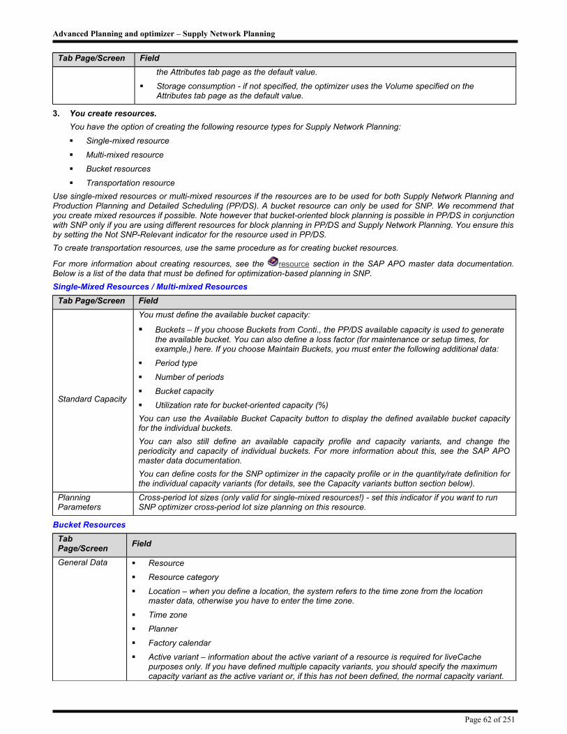
Advanced Planning and optimizer – Supply Network Planning

Tab Page/Screen Field

the Attributes tab page as the default value.

Storage consumption - if not specified, the optimizer uses the Volume specified on the Attributes tab page as the default value.

3. You create resources.

You have the option of creating the following resource types for Supply Network Planning:

Single-mixed resource

Multi-mixed resource

Bucket resources

Transportation resource

Use single-mixed resources or multi-mixed resources if the resources are to be used for both Supply Network Planning and Production Planning and Detailed Scheduling (PP/DS). A bucket resource can only be used for SNP. We recommend that you create mixed resources if possible. Note however that bucket-oriented block planning is possible in PP/DS in conjunction with SNP only if you are using different resources for block planning in PP/DS and Supply Network Planning. You ensure this by setting the Not SNP-Relevant indicator for the resource used in PP/DS.

To create transportation resources, use the same procedure as for creating bucket resources.

For more information about creating resources, see the resource section in the SAP APO master data documentation. Below is a list of the data that must be defined for optimization-based planning in SNP.

Single-Mixed Resources / Multi-mixed Resources

Tab Page/Screen Field

Standard Capacity

You must define the available bucket capacity:

Buckets – If you choose Buckets from Conti., the PP/DS available capacity is used to generate the available bucket. You can also define a loss factor (for maintenance or setup times, for example,) here. If you choose Maintain Buckets, you must enter the following additional data:

Period type

Number of periods

Bucket capacity

Utilization rate for bucket-oriented capacity (%)

You can use the Available Bucket Capacity button to display the defined available bucket capacity for the individual buckets.

You can also still define an available capacity profile and capacity variants, and change the periodicity and capacity of individual buckets. For more information about this, see the SAP APO master data documentation.

You can define costs for the SNP optimizer in the capacity profile or in the quantity/rate definition for the individual capacity variants (for details, see the Capacity variants button section below).

Planning Parameters

Cross-period lot sizes (only valid for single-mixed resources!) - set this indicator if you want to run SNP optimizer cross-period lot size planning on this resource.

Bucket Resources

Tab Page/Screen

Field

General Data Resource

Resource category

Location – when you define a location, the system refers to the time zone from the location master data, otherwise you have to enter the time zone.

Time zone

Planner

Factory calendar

Active variant – information about the active variant of a resource is required for liveCache purposes only. If you have defined multiple capacity variants, you should specify the maximum capacity variant as the active variant or, if this has not been defined, the normal capacity variant.

Page 62 of 251

Advanced Planning and optimizer – Supply Network Planning

Tab Page/Screen

Field

During the capacity check in interactive planning, the system considers the active variant. For more information, see the explanation of the Capacity Variants button.

Planning Parameters

Day -/Day + - The resource capacity’s validity period

Capacity overload (%)

Minimum load (%)

Cross-period lot size planning - Activate this indicator if you want to run an SNP optimizer cross-period lot size planning on this resource.

Standard Capacity

Period type

Number of periods

Bucket capacity

Utilization rate for bucket-oriented capacity (%)

Capacity Variants Button

Capacity variant

Valid from/to

Capacity utilization

Qty/rate definition

You can define multiple capacity variants and use a status indicator to label the available capacity of this variant as normal capacity, maximum capacity, or minimum capacity. You can define costs for using the normal or maximum capacity and for falling below the minimum capacity in the quantity/rate definition or the capacity profile of the resource. The SNP optimizer then takes these costs into account during planning. However, the SNP optimizer only takes into account the minimum available capacity and the costs you defined for a capacity variant with the status Normal Capacity for production resources.

You define the status indicator globally for all resources that have been assigned with the capacity variant. From the resource initial screen, choose Current Settings ® Capacity Variants. The default value is a maximum capacity (blank field). If you have defined multiple capacity variants with the same status, the system uses the smallest numbered variant.

We recommend that on the General Data tab page you always define the maximum capacity variant as the active variant or, if this has not been defined, the normal capacity variant.

The system includes the default available capacity for periods for which you have not created a capacity variant. If the normal capacity is below the minimum capacity, the system uses the normal capacity as the minimum capacity. If the normal capacity exceeds the maximum capacity, the system uses the normal capacity as the maximum capacity.

The SNP optimizer does not consider the Workdays field for planning. The optimizer considers the entries within this field when calculating the available capacity of the capacity variant but always uses the factory calendar for planning.

Definitions Button - the Quantities/Rates Tab Page

You use the Qty/Rate Definition to define the available capacity for the capacity variant.

Qty/rate definition (name)

Valid to

Planner

Number of periods

Period type

Bucket capacity

Unit

Costs – You define costs for falling below a minimum capacity or for using a normal or maximum capacity (you define costs for a capacity variant that you assign with status Minimum Capacity, Normal Capacity, or blank ( = maximum capacity). For more information, see the Capacity Variants Button section above. The optimizer only takes into account costs you define for a capacity variant with status Normal Capacity if the resource is a production resource.)

4. You assign resources to locations in the location master data.

Page 63 of 251

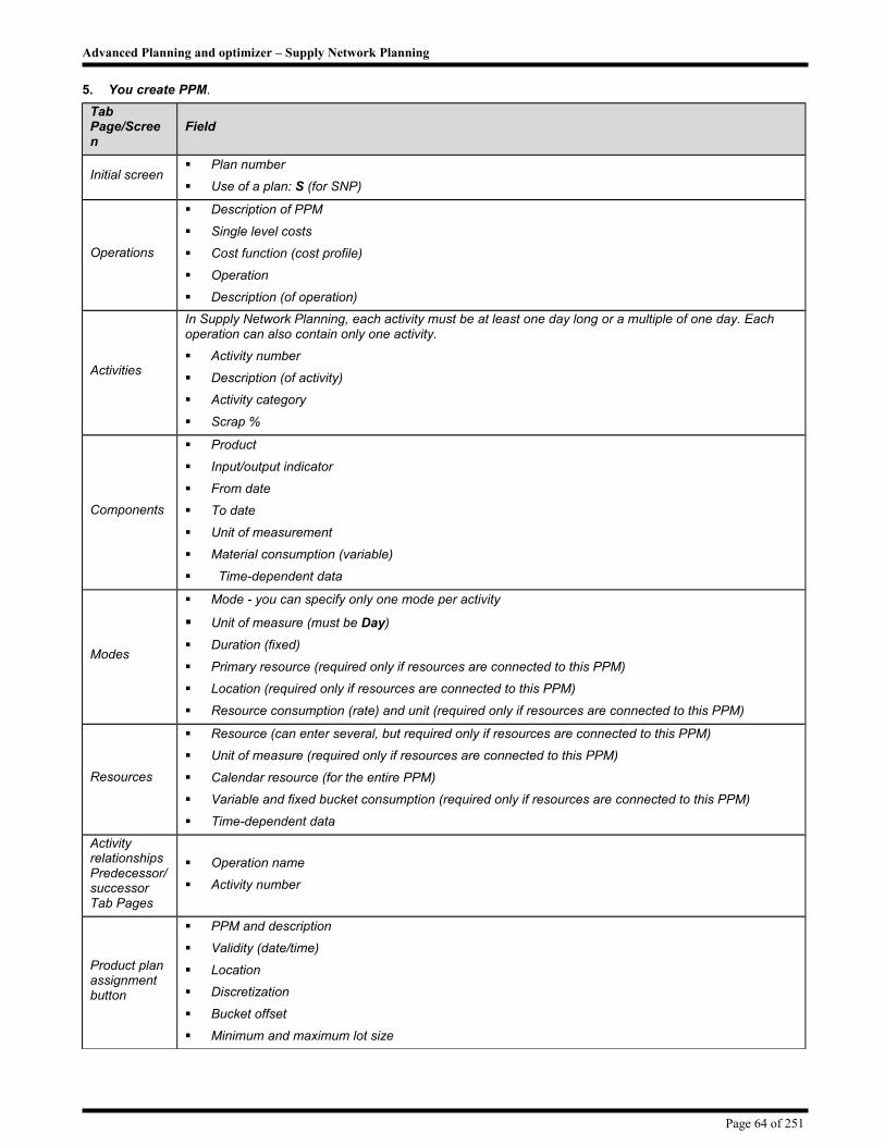
Advanced Planning and optimizer – Supply Network Planning

5. You create PPM.

Tab Page/Screen

Field

Initial screen Plan number

Use of a plan: S (for SNP)

Operations

Description of PPM

Single level costs

Cost function (cost profile)

Operation

Description (of operation)

Activities

In Supply Network Planning, each activity must be at least one day long or a multiple of one day. Each operation can also contain only one activity.

Activity number

Description (of activity)

Activity category

Scrap %

Components

Product

Input/output indicator

From date

To date

Unit of measurement

Material consumption (variable)

Time-dependent data

Modes

Mode - you can specify only one mode per activity

Unit of measure (must be Day)

Duration (fixed)

Primary resource (required only if resources are connected to this PPM)

Location (required only if resources are connected to this PPM)

Resource consumption (rate) and unit (required only if resources are connected to this PPM)

Resources

Resource (can enter several, but required only if resources are connected to this PPM)

Unit of measure (required only if resources are connected to this PPM)

Calendar resource (for the entire PPM)

Variable and fixed bucket consumption (required only if resources are connected to this PPM)

Time-dependent data

Activity relationships Predecessor/successor Tab Pages

Operation name

Activity number

Product plan assignment button

PPM and description

Validity (date/time)

Location

Discretization

Bucket offset

Minimum and maximum lot size

Page 64 of 251

Advanced Planning and optimizer – Supply Network Planning

Results

After you have configured the master data, you must set up the supply chain model in the Supply Chain Engineer, including the creation and maintenance of transportation lanes, before you can perform any planning runs.

Master Data Setup for the Heuristic

This section lists all the master data you have to create to run the heuristic successfully in Supply Network Planning. It lists all of the required fields and other data considered by the heuristic. Use this information as a checklist before you run the heuristic to make sure you have created all the master data for your supply chain model.

For detailed information, see the field-level help (F1 help). For more information, see the APO master data document.

If you want to work with local time zones, you have to set the Local Time Zone indicator in Model and Version Management. If you do not set this indicator, we recommend that you use the UTC time zone. When using local time zones, we also recommend that you use the same time zone for both the location and the planning calendar or for the location and the resource.

Process Flow

1. Create Locations (that are not product-dependent)

Location type

Storage resource

Handling resource

Calendar (production, shipping)

ATD category groups (for deployment, TLB)

Time zone

2. Create products

Tab page/screen

Field

Initial screen and header data

Lot size profile

Demand profile

SNP demand profile

SNP supply profile

Deployment profile

Base unit

Attributes Gross weight

Volume

Units of Meas.Define a conversion from the volume unit into the base unit of measure (based on the unit of measure of the planning area)

Lot size Procedure (lot-for-lot, fixed lot size etc.)

Safety stock method

SNP 2

SNP production horizon

SNP stock transfer horizon

These two horizons are also relevant if you are using Production Planning and Detailed Scheduling (PP/DS).

Procurement Procurement type

Planned delivery time (with external procurement)

GR/GI Handling capacity consumption

Storage consumption

3. Create Resources (optional).

You have the option of creating the following resource types for Supply Network Planning:

Single-mixed resource

Page 65 of 251

Advanced Planning and optimizer – Supply Network Planning

Multi-mixed resource

Bucket resource

Transportation resource

Use single-mixed or multi-mixed resources if you want to use the resources for both Supply Network Planning and Production Planning and Detailed Scheduling (PP/DS). Bucket resources can only be used for SNP. We recommend that you create mixed resources if possible. Note however that bucket-oriented block planning is possible in PP/DS in conjunction with SNP only if you are using different resources for block planning in PP/DS and Supply Network Planning. You ensure this by setting the Not SNP-Relevant indicator for the resource used in PP/DS.

To create transportation resources, use the same procedure as for creating bucket resources.

For general information about creating resources, see the resource section in the APO master data document. Below is a list of the exact data you have to define for heuristic-based planning in SNP.

Single / Multi-mixed Resources

Tab page/screen

Field

Standard Capacity

You must define the available bucket capacity:

Bucket definiton - if you choose From Cont. Capacity, the PP/DS available capacity is used to generate the available bucket capacity. You can also define a loss factor here (for maintenance or setup times for example). If you choose Maintain, you must enter the following additional data:

Period type

Number of periods

Bucket capacity

Rate of bucket-oriented capacity utilization (%)

You can use the Bucket Capacity button to display the available bucket capacity that was defined for the individual buckets.

You can also still define an available capacity profile and capacity variants, and change the periodicity and capacity of individual buckets. For more information, see the APO master data document.

Bucket Resources

Tab page/screen

Field

General Data

Resource

Resource category

Location – if you define a location, the system adopts the time zone from the location master data; if not, you have to enter the time zone

Time zone

Planner group

Factory calendar

Active variant

Reference resource

Planning Parameters

Day -/Day + - validity period for the resource capacity

Overload (%)

Minimum load (%)

Standard Capacity

Period type

Number of periods

Bucket capacity

Rate of bucket-oriented capacity utilization (%)

Capacity variants button

You can define up to 99 capacity variants in order to define the available capacity for specific validity periods.

Capacity variant

Page 66 of 251

Advanced Planning and optimizer – Supply Network Planning

Valid from/to

Rate of bucket-oriented capacity utilization (%)

Quantity/rate definition

The system takes into account the default available capacity for periods without a capacity variant.

Definitions button

You use the quantities/rates definition to define the available capacity for the capacity variant.

Qty/rate definition (name)

Valid to

Planner group

Number of periods

Period type

Bucket capacity

Unit

4. You assign resources to locations in location master data

5. You create PPM

Tab page/screen

Field

Initial screen Plan number

Use of a plan: S (for SNP)

Operations

Description of PPM

Operation

Description (of operation)

Activities

In Supply Network Planning, each activity must be at least one day long or a multiple of one day. Each operation can contain only one activity.

Activity number

Description (of activity)

Activity type

Scrap %

Components

Product

Input/output indicator

From date

To date

Unit of measure

Material consumption (variable)

Time-dependent data, if required

Modes

Mode - you can specify only one mode per activity

Unit of measure (must be Day)

Fixed duration

Primary resource (required only if resources are connected to this PPM)

Location (required only if resources are connected to this PPM)

Resource consumption (rate) and Unit (required only if resources are connected to this PPM)

Resources Resource (can enter several, but required only if resources are connected to this PPM)

Unit of measure (required only if resources are connected to this PPM)

Calendar resource (for the entire PPM)

Variable and fixed bucket consumption (required only if resources are connected to this PPM)

Page 67 of 251

Advanced Planning and optimizer – Supply Network Planning

Time-dependent data, if required

Activity relationships - Predecessor/successor tab pages

Operation name

Activity number

Product plan assignment button

PPM and description

Output product

Validity (date/time)

Location

Procurement priority

Period factor

Minimum and maximum lot size

6. You create transportation lanes in the Supply Chain Engineer or in master data.

Means of transport (using the Aggr. Planning key figure)

Transportation calendar

Procurement priority

For more information, see Supply Chain Model Set Up.

7. You have the option of creating quota arrangements in the Supply Chain Engineer or in master data.

Quota arrangement at location, external procurement relationship, or in-house production (PPM)

Quota arrangement (percentage)

If you do not define any quota arrangements, you must determine a procurement priority on the transportation lane, or in the PPM for automatic source determination. If both quota arrangements and procurement priorities have been defined, the heuristic includes the quota arrangements.

Result

Once you have set up the master data, you have to set up the supply chain model in the Supply Chain Engineer before you can perform any planning runs.

See also:

The APO master data documentation

The APO Supply Chain Engineer documentation

Master Data Setup for Supply & Demand Propagation

The master data fields that are supported by Supply & Demand Propagation are listed below.

Process Flow

1. You must enter the products and locations and assign the location products to a model.

2. You can enter the data, which should be taken into account during Supply & Demand Propagation, in the fields listed below:

Product Master

Tab Field

Attributes

Gross weight and unit

Volume and unit

SDP relevance (Optional field)

Product Location Master

Tab Field

Procurement Procurement type

The procurement type in the location product master is essential for Supply & Demand Propagation. By choosing a procurement type, you prioritize the various procurement options used in propagation. The options available are:

Page 68 of 251

Advanced Planning and optimizer – Supply Network Planning

E and no PPM: Check inventory first.

E and PPM: Check storage location first, then produce

F and no incoming transportation lanes: Check storage location first, then create external procurement

F and incoming transportation lanes: Check storage location first, then create stock transfer receipts

X and PPM and incoming transportation lanes: Check storage location first, then produce, then use stock transfer receipts

Other combinations using X: Analogous to E and F.

P: Check storage location first.

GR/GI

Optional Fields:

Goods rcpt time

Goods issue time

Hand l Cap consumption. GR and unit

Hand l Cap consumption. GI and unit

Master Data Setup for Aggregated Planning

In aggregated planning, you execute the SNP heuristic or the SNP optimizer at header location product level of a location product hierarchy. To do so, you must first have made the general master data settings for running the SNP heuristic or the SNP optimizer. For more information, see Master Data Setup for the Heuristic and Master Data Setup for the Optimizer. There are also some distinct features for aggregated planning described below that you must remember when defining the master data.

You must define all the master data at sub product level as well as at header product level. That means that the system cannot automatically generate the master data from sub product level.

In the following setting recommendations, the use of the word “should” means that planning can otherwise lead to incorrect or unexpected results.

Settings

Create Products and Locations

The following distinct features apply to aggregated planning:

You execute aggregated planning at header location product level. A header location product is the header product of a location product hierarchy that you have generated from a location hierarchy and a product hierarchy (see Create Hierarchies section). You create all the levels of these two-level hierarchies as standalone products and locations in the product and location master data.

If you want to plan multiple levels (locations) of your network, the same header products should be defined in all locations. There should not be any cycles in your network.

SNP disaggregation takes into account the rounding values and lot size parameters defined for the individual header and sub products. If you want to ensure that during SNP disaggregation there are no remainders at header product level, the rounding values defined at sub product level must be the same within a location product hierarchy. The rounding value of the header product must be a multiple of the value at sub product level. In addition, the minimum lot size at header level should be larger than or equal to the minimum lot size defined at sublevel.

The procurement type defined at header product level should also be supported at sub product level.

The same SNP production horizon, extended SNP production horizon, and SNP stock transfer horizon should be defined for all products of the location product hierarchy (including the header product).

Create Resources, PPM / PDS and Transportation Lanes

The following distinct features apply to aggregated planning:

If you carry out optimization-based planning with resources, you must also always create a resource at header product level. The SNP optimizer uses the resource and costs defined at header product level for aggregated planning. Creating resources is optional for the SNP heuristic.

To ensure that the resource consumption of fixed orders at sub product level is correctly taken into account during planning, you should note the following restrictions for creating resources:

You should use the same resources at header and sub product level. If you use a resource hierarchy, this restriction does not apply.

Page 69 of 251

Advanced Planning and optimizer – Supply Network Planning

The resource consumption of the production process models (PPMs) or production data structures (PDSs), and transportation lanes at header and sub product level should be similar.

The total of the resource capacities defined at header product level should form the resource capacity at sub product level. If you are using several PPMs/PDSs at sub product level, the resource consumption of the PPM/PDS at header product level should form the resource consumption of the different PPM/PDS’s at sub product level.

For external procurement, the same transportation lanes must apply for the header and sub products, since SNP aggregation and disaggregation use the source determination decisions from header product level.

Create Hierarchies

Standard hierarchy structures are already assigned to the standard planning area 9ASNP02. You can create hierarchies for location products, resources, and PPMs based on these structures. In SNP Customizing, you can also create your own hierarchy structures and assign them to your planning area. A standard hierarchy structure is also predefined for a PDS hierarchy. However, it is not assigned to the standard planning area 9ASNP02, so you have to assign it to your own planning area.

For more information, see the Implementation Guide (IMG) under Advanced Planning and Optimization → Master Data → Hierarchy → Define Hierarchy Structure.

Location Product Hierarchy

To create a location product hierarchy required for the standard aggregated planning process, first create a product hierarchy and a location hierarchy in the SAP-APO master data. You then generate a location product hierarchy from the product hierarchy and the location hierarchy. The header location product is at the top of a hierarchy tree of this hierarchy. The sub location products are at the second level. A hierarchy can consist of several hierarchy trees.

You can create the location product hierarchy as a location hierarchy for a product or as a product hierarchy for a location, for example. In the first instance, you must create a location hierarchy with one header location and multiple child locations as well as a product hierarchy. In this instance, the product hierarchy can only consist of one hierarchy level and must contain a sub product. In the second instance (in which you create a product hierarchy for a location), you have to do the opposite. In addition, when you define the hierarchy structure (see above), you must specify in the HierPos field the position in which the hierarchies will be in the generated location product hierarchy.

Example for Creating a Location Product Hierarchy

The figure shows the different possible combinations when you create a location product hierarchy. In this example, the product hierarchy consists of header product A with sub products B and C. The location hierarchy consists of header location 1 with sub location 2. In addition, there are location products A/1, A/2, C/2, and B/3, and location 3.

The generated location product hierarchy consists of the following levels: Header product/sub location level (level 1) and sub product/ sub location level (level 2). A/2 is located on level 1 and C/2 on level 2. C/2 is subordinate to A/2. A/1 is not a component of the generated location product hierarchy since the header product/header location level was not defined in the generated hierarchy. B/3 is not a component of the hierarchy since location 3 is not a component of the location hierarchy and nor are there any header product/sub location nodes for B/3 (which would then have to be called A/3).

PPM / PDS Hierarchy

For in-house production, you must also create a PPM or PDS hierarchy that contains its own hierarchy tree for each PPM or PDS at header product level, since SNP aggregation and disaggregation use the source determination decisions of the header product level. The PPM or PDS hierarchy should be consistent with the location product hierarchy.

Page 70 of 251

Advanced Planning and optimizer – Supply Network Planning

For more information about creating hierarchies, see the hierarchy section in the SAP APO master data documentation.

Resource Hierarchy

If you want to display the resource consumption at header level and you are not using the same resources at header and sub level in the PPMs or PDS, you should create a resource hierarchy so that the resource consumption is displayed correctly. This hierarchy should be consistent with the PPM/PDS hierarchy used.

Master Data Setup for Safety Stock Planning

This document describes which specific master data you must define for safety stock planning in Supply Network Planning (SNP). For more information, see the associated F1 Help.

Process

1. Determine whether you want to use standard or extended safety stock planning.

2. If you use standard safety stock planning, enter the relevant data in the following fields on the Lot Size tab page in the location product master:

Safety Stock Method – Methods SB, SZ, SM for time-independent determination and methods MB, MZ, MM for time-dependent determination.

Safety Stock - is considered by the system during safety stock methods SB and SM.

Safety Days’ Supply - Considered by the system during safety stock methods SZ and SM.

3. If you use extended safety stock planning, enter the relevant data in the following fields on the Lot Size tab page in the location product master:

Safety Stock Method – Methods AT, AS, BT and BS.

Service Level (%)

Demand Forecast Err. (%) – Can also be calculated by the system using historical data.

RLT Forecast Error (%)– Can also be calculated by the system using historical data.

Target Days’ Supply – During safety stock methods AT and BT the system interprets this value as an order cycle. During safety stock method BS the system uses this value to calculate the purchase order quantity.

Replens. Lead Time – Can also be calculated by the system using historical data.

Min. SFT

Max. SFT

Master Data Setup for the Deployment Heuristic

This section lists the master data you have to create to run the deployment heuristic successfully in Supply Network Planning (SNP). It lists all of the required fields and other data considered by deployment. Use this information as a checklist before you run deployment to make sure you have maintained all the master data for your supply chain model.

For more information, see the SAP APO master data documentation.

Process Flow

1. Create locations (choose the SNP tab page in the location master)

ATD receipt

ATD issue

You can define these fields in the location master as well as the location product master. During the deployment run, the system first checks whether the category group is specified for the location product. If not, the system checks the entry at location level. If no category group is defined for the location either, the system uses the standard category groups ATR or ATI.

You define category groups in the Customizing for SNP under Basic Settings → Maintain Category Groups.

Push not allowed

You set this indicator to restrict the locations to which the system distributes the supply available during deployment. For example, you may not wish to push supply to a location that has low demand.

2. Create products

Deployment profile

If you choose fair share rule C or push rule Q, the system uses the quota arrangements defined in the Supply Chain Engineer (SCE); therefore, you must also define the quota arrangements when you set up the supply chain model.

Page 71 of 251

Advanced Planning and optimizer – Supply Network Planning

SNP supply profile

SNP demand profile

SNP 2 tab page

ATD receipt

ATD issue - (see above)

Lot Size tab page

Maximum lot size

Rounding value

If you have assigned an SNP lot size profile for transportation lanes to the relevant transportation lane, the system first takes into account the rounding data that you have defined in this profile.

The deployment heuristic does not consider the minimum lot size or the rounding profile, which you can define on the Lot Size tab page in the location product master data, as well as in the SNP lot size profile for transportation lanes.

Note in addition that deployment heuristic values generally round down.

Result

After you have set up the master data, you must set up the supply chain model in the Supply Chain Engineer before you can execute a planning run. This includes creating and maintaining transportation lanes.

See also:

The SAP APO master data documentation

Supply Chain Model Setup

Master Data Setup for the Deployment Optimizer

This section lists all the master data you have to create to successfully run the deployment optimizer in Supply Network Planning. It lists all of the required entry fields and other data that the deployment optimizer considers. Use this information as a checklist before you run the deployment optimizer to make sure you have maintained all the master data for your supply chain model.

For more information, see the SAP APO master data documentation.

If you want to work with local time zones, you have to set the Local Time Zone indicator in Model and Version Management. If you do not set this indicator, we recommend that you use the UTC time zone. When using local time zones, we also recommend that you use the same time zone for both the location and the planning calendar or for the location and the resource.

Process Flow

1. Create Locations (that are not product-dependent)

Location type

Storage resource

Handling resource

Calendar

ATD category groups (for deployment and the TLB); if you do not make any entries, the optimizer uses default values

Time zone

2. Create products

Tab Page/Screen Field

Header data Base unit

Properties

Gross weight and unit

Volume and unit

Shelf life

Units of Meas.Define a conversion from the volume unit into the base unit of measure (based on the unit of measure of the planning area)

SNP 1 Penalty costs for customer demand, the demand forecast, and the corrected demand forecast (required only for products that fulfill demand; not required for components):

Page 72 of 251

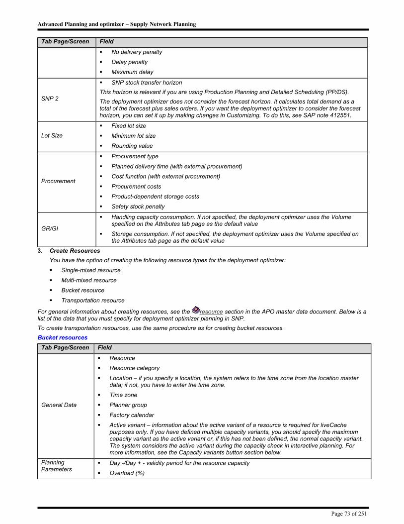
Advanced Planning and optimizer – Supply Network Planning

Tab Page/Screen Field

No delivery penalty

Delay penalty

Maximum delay

SNP 2

SNP stock transfer horizon

This horizon is relevant if you are using Production Planning and Detailed Scheduling (PP/DS).

The deployment optimizer does not consider the forecast horizon. It calculates total demand as a total of the forecast plus sales orders. If you want the deployment optimizer to consider the forecast horizon, you can set it up by making changes in Customizing. To do this, see SAP note 412551.

Lot Size

Fixed lot size

Minimum lot size

Rounding value

Procurement

Procurement type

Planned delivery time (with external procurement)

Cost function (with external procurement)

Procurement costs

Product-dependent storage costs

Safety stock penalty

GR/GI

Handling capacity consumption. If not specified, the deployment optimizer uses the Volume specified on the Attributes tab page as the default value

Storage consumption. If not specified, the deployment optimizer uses the Volume specified on the Attributes tab page as the default value

3. Create Resources

You have the option of creating the following resource types for the deployment optimizer:

Single-mixed resource

Multi-mixed resource

Bucket resource

Transportation resource

For general information about creating resources, see the resource section in the APO master data document. Below is a list of the data that you must specify for deployment optimizer planning in SNP.

To create transportation resources, use the same procedure as for creating bucket resources.

Bucket resources

Tab Page/Screen Field

General Data

Resource

Resource category

Location – if you specify a location, the system refers to the time zone from the location master data; if not, you have to enter the time zone.

Time zone

Planner group

Factory calendar

Active variant – information about the active variant of a resource is required for liveCache purposes only. If you have defined multiple capacity variants, you should specify the maximum capacity variant as the active variant or, if this has not been defined, the normal capacity variant. The system considers the active variant during the capacity check in interactive planning. For more information, see the Capacity variants button section below.

Planning Parameters

Day -/Day + - validity period for the resource capacity

Overload (%)

Page 73 of 251

Advanced Planning and optimizer – Supply Network Planning

Tab Page/Screen Field

Minimum load (%)

Finite scheduling – is used for lot size planning, that is, the set up status from Production Planning and Detailed Scheduling

Standard Capacity

Period type

Number of periods

Bucket capacity

Rate of bucket-oriented capacity utilization (%)

Capacity variants button

Capacity variant

Valid from/to

Rate of bucket-oriented capacity utilization (%)

Quantity/rate definition

You can define multiple capacity variants and use a status indicator to label the available capacity of this variant as normal capacity, maximum capacity, or minimum capacity. You can define costs for using the normal or maximum capacity and for falling below the minimum capacity in the quantity/rate definition or the capacity profile of the resource. The deployment optimizer then takes these costs into account during planning. However, the optimizer only takes into account the minimum available capacity and the costs you defined for a capacity variant with the status Normal Capacity for production resources.

You define the status indicator globally for all resources that have been assigned with the capacity variant. From the resource initial screen, choose: Current Settings ® Capacity Variants. The default value is a maximum capacity (blank field). If you have defined multiple capacity variants with the same status, the system uses the smallest numbered variant.

We recommend that on the General Data tab page you always define the maximum capacity variant as the active variant or, if this has not been defined, the normal capacity variant.

The system includes the default available capacity for periods that you have not created a capacity variant for. If the normal capacity is below the minimum capacity, the system uses the normal capacity as the minimum capacity. If the normal capacity exceeds the maximum capacity, the system uses the normal capacity as the maximum capacity.

The deployment optimizer does not consider the Workdays field for planning. The optimizer does consider the entries within this field when calculating the available capacity of the capacity variant but always uses the factory calendar for planning.

Definitions button – the Quantities/Rates tab page

You use the Qty/Rate Definition to define the available capacity for the capacity variant.

Qty/rate definition (name)

Valid to

Planner group

Number of periods

Period type

Bucket capacity

Unit

Costs – You define costs for falling below a minimum capacity or for using a normal or maximum capacity (you define costs for a capacity variant that you assign with status: Minimum Capacity, Normal Capacity, or blank ( = maximum capacity) – for details, see the Capacity variants button section above. The optimizer only takes into account costs you define for a capacity variant with status Normal Capacity if the resource is a production resource.)

4. Assign resources to locations in location master data

Result

After you have set up the master data, you must set up the supply chain model in the Supply Chain Engineer before you can execute a planning run. This includes creating and maintaining transportation lanes.

Page 74 of 251

Advanced Planning and optimizer – Supply Network Planning

Master Data Setup for the Transport Load Builder

In addition to the general master data settings for planning in Supply Network Planning (SNP), or in the SAP Inventory Collaboration Hub (SAP ICH), you can also make additional settings for the Transport Load Builder (TLB). The following is intended to provide an overview of the TLB settings. For more information, see the F1 Help for the individual fields.

For more information on the master data settings that you can make for the additional TLB settings in SAP ICH, see Additional TLB Functions in SAP ICH.

Settings

Product Master Data

You make the following settings in the product, or location product, master data:

Tab Field

Properties

Stacking Factor

This fields is relevant if you want to use the Pallet Positions TLB parameter in the TLB profile

The stacking factor indicates how many pallets of a product can be stacked on top of each other. For mixed pallets, the system uses the smallest stacking factor of all products.

Units of Meas.For the parameters, weight, volume, and pallet positions (only SNP TLB) that you use in the TLB profile, you must determine conversion of the parameter unit of measure into the base unit of measure for the product.

SNP 2

VMI Purchasing. Group.

The TLB can divide the TLB shipments into individual orders according to the purchasing group of the VMI customer.

ATD Receipt and ATD Issue

These fields are only considered by the SNP TLB. You can enter the category groups that you have defined in the SNP Customizing under Basic Settings ® Maintain Category Groups. Using the category groups, you define which order categories are included in the quantity that is available for transport load building.

If you do not enter a value here, the system uses the value from the location master data or the standard category groups ATR and ATI.

Lot Size/Quantity and Date Determination

Rounding value

The TLB uses the rounding value for building transport loads. However, the TLB first uses the value that you have defined in the transportation lane, that is, in the lot size profile (SNP) or transportation guideline set (SAP ICH). If no value is assigned, the TLB then uses the value specified here or 1.

So that the SNP TLB can use this rounding value, you must set the relevant indicator in the SNP Customizing under Basic Settings ® Maintain Global SNP Settings. Otherwise, the SNP TLB uses the rounding value from the transportation lane.

GR/GI

Handling unit G

The TLB can only pack products with the same handling unit group together in the same handling unit (HU). In the SNP TLB, which does not use handling units, this field applies to pallets.

Max. Coverage

The TLB considers the maximum coverage time during shipment upsizing. The system only brings forward as many deployment stock transfers as are necessary to cover demand within this time period.

Shipment Upsizing

For the location product, you specify whether shipment upsizing is allowed and whether is is permitted beyond the maximum coverage time period.

Loading Group

The TLB considers the loading group for the straight loading method.

Not Palletable

You specify whether the location product may be stacked on pallets. If you set this indicator, the TLB considers no pallet positions for this product.

Location Master Data

You make the following settings in the location master data:

Page 75 of 251

Advanced Planning and optimizer – Supply Network Planning

Tab Page/Screen Field

Initial screen

Loc. Type

This field is relevant if you want to use transportation zones. For more information, see Use of Transportation Zones.

SNP ATD Receipt and ATD Issue

If you have not defined category groups for the location product (see above), the SNP TLB considers the category groups defined here.

Transportation Lane Master Data

You make the following settings for the means of transport in the transportation lane master data:

Section Field

Means of Transport

TLB Profile

You must assign a TLB profile that you created previously.

Loading Method

You specify whether you want the TLB to consider the straight loading oder load balancing loading method.

Pull-In Horizon

If the TLB carries out a shipment upsizing, it considers the pull-in horizon.

Siz.Desn and Shpmt Thr.Val.

In the Siz.Decsn field, you determine how the TLB calculates the value it uses to decide about shipment sizing. The system compares the base value calculated with the value you have entered in the Shpmt Thr.Val field, and then carries out shipment upsizing or downsizing.

Product-specific transportation

T. Lot Prfl

The SNP TLB only considers this field. You can enter a profile here that you created in the SNP Customizing under Basic Settings ® Profiles ® SNP-Lot Size Profile (Transportation Lane). The TLB considers the value defined in this profile (see above).

Model/Version Creation

In this process, you create a model name and assign the model to a planning version so that you can you can model the supply chain in the Supply Chain Engineer in the next step. You must define the model name before you can set up the supply chain model.

Creating multiple versions of the model allows you to perform simulative planning and what-if scenarios without corrupting the supply chain model.

Only the active version receives data from R/3 via CIF.

Process Flow

1. Create a model name and give it a description.

2. Assign the model to at least one planning version

Planning version name and description

SNP: Change planning active (set flag to active)

PP/DS: Change planning active (set flag to active)

If you use PP/DS, you must set the PP/DS: Change planning active and SNP: Change planning active indicators to enable automatic planning to be triggered or planning file entries to be created when changes relevant to planning occur. These indicators are important when converting Supply Network Planning orders into PP/DS orders and vice-versa. You must set these indicators for the target-planning version; otherwise you will have to plan all orders manually.

Planning Version Merge

You use this function to copy selected Supply Network Planning (SNP) key figures that you planned in an APO planning version (copy of the active version) back into the active version. You can limit your selection to location products and SNP planners.

Page 76 of 251

Advanced Planning and optimizer – Supply Network Planning

Multiple SNP planners can first make copies of the active version’s master data and transaction data:

The SNP planners then revise these copies within their individual planning environments. Each SNP planner has his or her own planning section (product and location):

The SNP planners then copy the revised planning versions back into the active version:

You have to ensure that the plans of the various SNP planners do not overlap since, when the individual planning versions are copied back into the active version, the version that is copied back last overwrites the data from all the previously copied versions.

Prerequisites

You have created one or more copies of the active version (000) as planning versions.

An SNP planner has been assigned to all the location products in master data.

Page 77 of 251

Advanced Planning and optimizer – Supply Network Planning

You have authorization for the relevant locations and products to copy the data from the planning version back into the active version (authorization object C_APO_PLNR). The SNP planner controls authorization.

Features

You can use this function to copy four SNP key figures from a planning version back into the active version. PP/DS order data cannot be copied. The following is a list of the SNP key figures:

Planned Production (key figure 9APPROD, key figure function 2001)

SNP Distribution Receipt (key figure 9APSHIP, key figure function 4001)

Deployment Distribution Receipt (key figure 9AFSHIP, key figure function 4005)

Safety Stock (key figure function 3003)

Selection of SNP Key Figures

You choose the SNP key figures that you want to copy back into the active version in transaction /SAPAPO/VERMER:

Planning area: Indicates the SNP planning area that key figures are to be copied from into the active version.

Key figures: Indicates the SNP key figures that are to be copied back.

Planning version (source): Name of the planning version to be copied back.

Planning version (target): Name of the active version. You cannot modify this entry.

Product: Name of one or more location products whose previously chosen key figures are to be copied back. This entry is optional. If you do not make an entry here, the key figures of all the location products that you are authorized to use and that belong to the underlying model are copied back.

Location: Limits you to specific locations whose location products the key figures are to be copied back from. This entry is optional. If you do not make an entry here, the key figures of the location products you are authorized to use are copied back from all locations belonging to the underlying model.

Planner: Limits you to specific SNP planners whose assigned location products the key figures are to be copied back from. This entry is optional. If you do not make an entry here, the key figures of the assigned location products you are authorized to use are copied back for all SNP planners belonging to the underlying model.

The copying of planning versions back to the active version is not a copy process in the strict sense of the word. In fact, the SNP key figures concerned are first deleted from the active version and then recreated in it from the planning versions.

Log File Creation

The system generates a log file for storing messages about the copy process. If you run this process online, the log file is displayed automatically once the copying is complete.

If you run the process in the background, the log file is created but not displayed. You can then call it up using the identification numbers from the job log.

Log file creation is activated by the system and cannot be deactivated.

Do Not Permit Errors

If this option is set, copying can only proceed if all objects can be copied without errors. If you do not set this option, it is possible that not all of the objects will be copied.

Test Run

The system runs the entire copy process as a simulation without actually copying the data into the active version. It runs through all stages of the copy process (authorization checks, log file creation, and so on) apart from the final copy into the active version. To then start the actual copy process, remove the Test Run indicator.

Stop CIF Queues

If this option is set, the system stops all data transfers from R/3 systems into the SAP APO system through the Core Interface before starting the copy process. Only inbound queues in the same system are stopped. You have to stop outbound queues in the source system

During the copy process, stop Core Interface (CIF) using either this function, the monitor, or a background job in order to prevent lock problems from occurring.

To stop CIF queues, you need authorization object S_ADMI_FCD.

Constraints

SNP orders are not permitted to be published directly into the SAP R/3 system. Communication with the SAP R/3 system is only permitted to take place using the Production Planning and Detailed Scheduling (PP/DS) component. The system performs a technical check of the corresponding Customizing for this.

Page 78 of 251

Advanced Planning and optimizer – Supply Network Planning

It is not permitted for any releases to be made into or out of SNP until all the planning versions that came from an active version have been copied back into this active version. In particular, no order is permitted to be converted for PP/DS and no data can be transferred into the active version from Demand Planning.

An authorization check is made during the copy process. You can only copy key figures for location products whose SNP planner is assigned to your user.

The copy process ignores scheduling agreement schedule lines.

Activities

1. Start transaction: Supply Network Planning → Environment → Planning Version Merge (/SAPAPO/VERMER).

2. Enter the necessary SNP key figures, planning version, and required restrictions (product, location, SNP planner).

3. If required, set the following options:

Do Not Permit Errors

Test Run

Stop CIF Queues

Choose Execute to start the function.

4. Choose Supply Network Planning → Environment → Planning Version Merge: Message Log to display the log file.

You can also call up the log file directly from transaction /SAPAPO/VERMRM.

Supply Chain Model Setup

The supply chain model consists of individual nodes (locations) and links (transportation lanes). You can assign several different planning versions to a model. It is also possible to create multiple models for simulation purposes.

Only the active version receives data from the R/3 system through the Core Interface (CIF).

Prerequisites

You have to set up the master data for planning in accordance with how you are using this model:

Locations

Resources

Products

PPMs

For more information, see the corresponding SNP documentation sections on setting up master data for the individual planning methods (the heuristic, the optimizer, and so on).

Process Flow

1. You create a model and assign objects to it that you want in your model:

Locations

Resources

Products

PPM

For more information, see APO Model Maintenance.

2. Add transportation lanes to the model. For general information about creating transportation lanes, see Transportation Lane Maintenance. The SNP-relevant fields are listed below:

Header data:

Transportation planner

The product procurement area:

Procurement priority (heuristic and deployment only)

Distribution priority (deployment only)

From and to lot sizes (heuristic only)

External procurement relationship data (transferred using CIF – this is relevant when working with scheduling agreements)

The means of transport area:

Page 79 of 251

Advanced Planning and optimizer – Supply Network Planning

Aggregated planning (indicator must be set)

Transportation calendar

Transportation duration

Additional retention period

Transportation distance

Transportation costs (optimizer only)

Cost function (optimizer only)

TLB profile (for the Transport Load Builder)

Bucket offset (optimizer only)

Period factor (heuristic only)

Discrete means of transport (optimizer only)

The product-specific means of transport section:

Transportation costs (optimizer only)

Consumption (of transportation resource)

SNP lot size profile for transportation lanes

Stacking factor (for the Transport Load Builder)

3. You maintain quota arrangements, if required. For more information about the role of quota arrangements in supply

source determination within the SNP heuristic, see Source Determination (Heuristic). The optimizer creates quota

arrangements automatically during the planning run. For more information about creating quota arrangements, see Quota Arrangement Maintenance.

Production Data Structure in SNP

Structure containing the master data for planning in SAP APO. Production data structures vary in the following ways:

Origin:

Generated from iPPE data (product structure, process structure, factory structure)

Generated from SAP R/3 data, that is, classical master data, such as bill of materials, phantom assembly, work plan, and master recipe.

In both cases, the production version serves as the basis for generating the production data structure.

Application:

Demand Planning (DP)

Supply Network Planning (SNP)

Capable-to-Match Planning (CTM)

Production Planning and Detailed Scheduling (PP/DS)

In SAP APO, the production data structure is used as a source of supply.

Use

In Supply Network Planning, you can use the production data structure as an alternative to the production process model (PPM) Similar to the PPM, the PDS is a combination of the work plan and the bill of materials. Compared to the PPM, the PDS offers more flexible ways of combining and reusing data from individual work plans and bills of materials.

The SNP PDS is supported by all SNP planning processes, except for demand and stock propagation. There is a further restriction for the Delete Transaction Data function. With this function, you cannot select or delete according to specific PDSs.

The following options are available for creating an SNP production data structure:

Generation of an SNP Production Data Structure from iPPE Data

You can either create the iPPE data in a connected DIMP system, and then transfer it to an SAP SCM system using the APO Core Interface (CIF), or you can create the data directly in the SAP SCM system. Note that, for SNP, you must use an SNP work plan in the iPPE data. You then create a product version for the iPPE data, and generate an SNP production data structure from there.

Page 80 of 251

Advanced Planning and optimizer – Supply Network Planning

You determine the validity of a product and a location in the production version, as in a PPM or an SAP R/3 production version. You can also define costs and enter co-products. If necessary, you can also specify a PP/DS production version in the production version, which is considered by PP/DS when converting SNP orders into PP/DS orders.

Generation of an SNP Production Data Structure from SAP R/3 Data

You can generate the SNP PDS directly from work plan, bill of materials, and production version data in SAP R/3. To do this, you must select SNP or SNP Subcontracting as the PDS type in the CIF integration model. The relevant SAP R/3 data is then transferred to the SAP SCM system automatically, and an SNP PDS is then generated from it in the SAP SCM system.

If you select SNP Subcontracting, the master data (also for components) is automatically created at the subcontractor location. The transportation lane between plant and subcontractor is also generated automatically (this is not possible when using SNP PPM).

You can also influence the generation of a SNP PDS from SAP R/3 data with the following Business Add-Ins (BAdIs).

/SAPAPO/CURTO_SNP: You can calculate bucket consumption of resources with the CALC_BUCKET_CONSUMPTION method of this BAdI. This method, which executes standard calculation of bucket consumption, is active automatically.However, you can change the calculation.

/SAPAPO/CULLRTOSNP: If you want to carry out optimization-based SNP planning, you can use the FILL_COST_FIELDS method of this BAdI to fill the SNP PDS cost fields.

You can use both BAdIs to change the SNP PDS data to be generated.

Once an SNP PDS has been generated, you can only display that source of supply. You can make changes in the iPPE or SAP R/3. You must then, however, regenerate the PDS.

The SNP PDS is used in SNP like the SNP PPM. The source determination considers all existing sources of supply, irrespective of whether it concerns an SNP PPM or an SNP PDS.

Note that most SNP PPM procedures also apply for the SNP PDS. This is not always explicitly mentioned in SNP documentation

You cannot generate an SNP PDS from Production Planning and Detailed Scheduling structures (PP/DS PDS).

The SNP PDS can also be used in CTM planning.

See also:

For more information, see the SAP APO master data documentation entitled Production Data Structure and Integrated Product and Process Engineering (iPPE)

Generating SNP PPMs from PP/DS PPMs

SAP APO allows you to generate SNP production process models (PPMs) based on existing PP/DS PPMs. For instance, this may be a good idea if you are using both Production Planning and Detailed Scheduling (PP/DS) and Supply Network Planning and after the SNP planning want to convert SNP orders into PP/DS orders. During order conversion, the system is then able to automatically determine the correct PP/DS PPM mode combination that is appropriate for the SNP order. The following is a list of the generation options available:

• SNP PPM generation with lot size margin:

You use this generation function to generate SNP PPMs from PP/DS PPMs for lot size margins and several mode combinations of a PP/DS PPM. The system creates an SNP PPM per PP/DS PPM mode combination. For more information, see SNP PPM generation with lot size margin.

As the number of mode combinations and therefore also the number of SNP PPMs will possibly become very large depending on the number of activities and alternative PP/DS PPM modes, you can choose specific PP/DS PPM mode combinations for the SNP PPM before the function is run or enter specific parameters to restrict the SNP PPMs generated. For more information, see specifying mode combinations for SNP PPM generation.

SNP PPM generation without lot size margin:

You use this generation function to generate SNP PPMs from PP/DS PPMs for one individual lot size and exactly one PP/DS PPM mode combination. Each generation report run can generate exactly one SNP PPM corresponding to one specific PP/DS PPM mode combination. For more information, see SNP PPM generation without lot size margin.

For example, you can use this function when SNP PPM generation with lot size margins is not possible.

SNP PPM Generation With Lot Size Margin

You use the SNP PPM Generation With Lot Size Margin function to generate SNP production process models (PPMs) from PP/DS PPMs for lot size margins and multiple mode combinations of a PP/DS PPM. Due to the fact that PP/DS PPMs can

Page 81 of 251

Advanced Planning and optimizer – Supply Network Planning

have multiple modes defined per activity whereas SNP PPMs can only have one mode per activity, the system generates one SNP PPM per PP/DS PPM mode combination.

Integration

It is possible that the number of mode combinations and therefore also the number of SNP PPMs generated will become very large, depending on the number of activities and alternative PP/DS PPM modes. For this reason, there is a different function available that you use before running this function to select certain PP/DS PPM mode combinations or enter parameters in order to restrict the number of SNP PPMs generated. You then flag the chosen PPM plans so that they are considered the next time this function is executed. For more information, see Specifying Mode Combinations for SNP PPM Generation.

You can also run the function described here directly without first defining the mode combinations. Parameters are available on the selection screen for this function, which you use to restrict the number of SNP PPMs generated. However, manual preselection of mode combinations is only possible in the function mentioned above.

Prerequisites

In the system, you have created the appropriate PP/DS PPMs from which you want to generate the SNP PPMs. For more

information, see the PPM Plan section of the APO master data document.

During generation, the system only takes into account multi mixed resources or single mixed resources that have not been set with the indicator Not SNP Rel. on the Planning Parameters tab page from resource master data. Also, the system only takes into account products with the activated SDP relevance indicator on the Properties tab page within product master data.

Activities

1. You maintain the control parameters for executing the function. From the SAP APO Easy Access menu, choose Master Data Production Process Model SNP PPM Generation With Lot Size Margin.

On the selection screen, if you leave the PP/DS plan number and SNP plan number fields blank, the flagged PPM plans and associated control parameters are adopted from the transaction SNP PPM Generation: Determine Mode Combinations. On the selection screen, if you specify a specific PP/DS plan number and SNP plan number, you must also enter the associated control parameters on the screen. If you do not enter any values, the system uses the maximum values possible.

For example, you use the control parameters to specify how the operations, activities, and resource consumption from the PP/DS PPM are transferred to the SNP PPM that has been setup for bucket-oriented SNP planning. You can also restrict the number of SNP PPMs generated by limiting the PP/DS PPM mode combinations considered.

The following control parameters are available:

Parameter Use

Start Date of Generation Period

You use this date to specify when bucket generation for the SNP PPM plan is to start. The temporary PP/DS order created by the system, from which the SNP plan is to be generated, is also scheduled from this start date on.

If possible, you should choose the start date so that the PPM generation horizon corresponds to a typical horizon for your work processes (based on leave periods, public holidays, and so on).

For generation, it is not possible to shift the start date into the past.

Bucket Size

You use bucket size (period length) to specify which PP/DS plan activities are to become an SNP plan activity during SNP plan generation. To do this, a temporary PP/DS order over a certain lot size (typical order lot size, see below) is created by forward scheduling from the Start Date of the Generation Period specified. All activities from the planned order that fall within a bucket of the pre-specified size, then become one production activity in the generated SNP plan. This means that the longer the bucket is, the more PP/DS plan activities can be included within one SNP plan activity. This production activity is one day long. If necessary, the remaining time from the bucket is occupied by a wait activity.

You should choose the bucket size so that it corresponds to the period length for SNP planning (that is, the period length specified in the planning buckets profile).

Lowest Mode Priority

You use lowest mode priority to specify which PP/DS plan modes are to be considered for the mode combination, that is, how many SNP plans are generated. Modes with a lower priority than the one specified here are not considered for SNP plan generation.

Consumption Calculation

You use the consumption calculation parameter to specify how the variables and fixed bucket resource consumptions from SNP plan activities are to be calculated, which means how the corresponding PP/DS plan consumptions are to be transferred to the SNP plan. There are the following two types of calculation:

1. Consumption is calculated on a one to one basis, so that one PP/DS order corresponds to one SNP order (generation variant without PP/DS campaign):

The system uses the fixed duration and fixed resource consumption from the PP/DS plan plus the

Page 82 of 251

Advanced Planning and optimizer – Supply Network Planning

Parameter Use

duration of sequence-dependent setup activities to calculate the fixed bucket consumption of the SNP plan. The duration of these activities is calculated as the setup duration of an initial setup group/setup key (as specified in the setup matrix) to the setup group/setup key of the operation considered. Variable bucket consumption is determined from the PP/DS plan variable duration and variable resource consumption.

2. Consumption is calculated on a many to one basis, so that n PP/DS orders correspond to one SNP order (generation variant with PP/DS campaign):

The system calculates fixed bucket consumption from the duration of sequence-dependent setup activities only (see above). The fixed PP/DS plan durations are made linear and go into the variable bucket consumptions from the SNP plan. Variable durations and resource consumptions are also used to determine the variable bucket consumption.

Typical Order Lot Size

This is the lot size over which the system creates a temporary PP/DS order. The system uses the temporary PP/DS order to assign PP/DS PPM operations to the respective SNP buckets (periods) using normal scheduling rules.

As the order length is usually based on the lot size, you should enter the typical order lot size in this field. When choosing this lot size, it should correspond to the typical SNP lead time, because all orders that you create from the generated SNP PPM receive the duration derived from the temporary PP/DS order.

As a rule, the larger the typical order lot size, the longer the duration of activities in the generated SNP PPM. Note that if you choose an order lot size that is too large, the duration of activities may exceed the bucket size, and the system will not be able to generate an SNP PPM. Because of this, there are several options available for determining the typical order lot size (see the selection help).

Maximum Number

You use this parameter to specify an upper limit on the number of SNP plans to be generated.

If this number is exceeded, the system terminates generation.

2. You run the function.

3. The system generates SNP PPMs from the specified PP/DS PPMs according to the parameters you defined.

4. It is possible to view the results of the function and messages in a log. From the SAP APO Easy Access menu, choose Master Data Production Process Model SNP PPM Generation: Display Log.

Specifying Mode Combinations for SNP PPM Generation

You use this function before running SNP PPM Generation with Lot Size Margin to choose certain PP/DS PPM mode combinations for the SNP-PPMs or to enter specific parameters in order to restrict the number of SNP PPMs generated. Because the automatic generation function generates exactly one SNP PPM per PP/DS PPM mode combination, it is possible that the number of SNP PPMs generated will become very large, depending on the number of activities and alternative PP/DS PPM modes. After you have made your selection, you can flag the PPM plans so that they are part of the next run of SNP Generation with Lot Size Margin.

This function can also be used to change the mode combinations and parameters for SNP PPM plans that have already been generated by the SNP PPM Generation with Lot Size Margin function (for example, you can choose new mode combinations), and then flag the plans for a new generation report run.

Prerequisites

In the system, you have created the appropriate PP/DS PPMs from which you want to generate the SNP PPMs. For more

information, see the PPM Plan section of the APO master data document.

During generation, the system only takes into account multi mixed resources or single mixed resources that have not been set with the indicator Not SNP Rel. on the planning parameters tab page from resource master data. Also, the system only takes into account products with the activated SDP relevance indicator on the Properties tab page within product master data.

Procedure

1. From the SAP APO easy access menu, choose Master Data Production Process Model SNP PPM Generation: Determine Mode Combinations. The Select Worklist screen appears.

2. In the upper part of the screen, specify a PP/DS PPM plan or range of PP/DS plans that you want to convert into SNP PPM plans using the SNP Generation with Lot Size Margin function (you can also choose PP/DS plans by entering one or more products or location products). Alternatively, in the lower part of the screen, you specify SNP plans that have already been generated with the SNP PPM Generation with Lot Size Margin function, which you want to change and flag to be run in a new generation report run.

Page 83 of 251

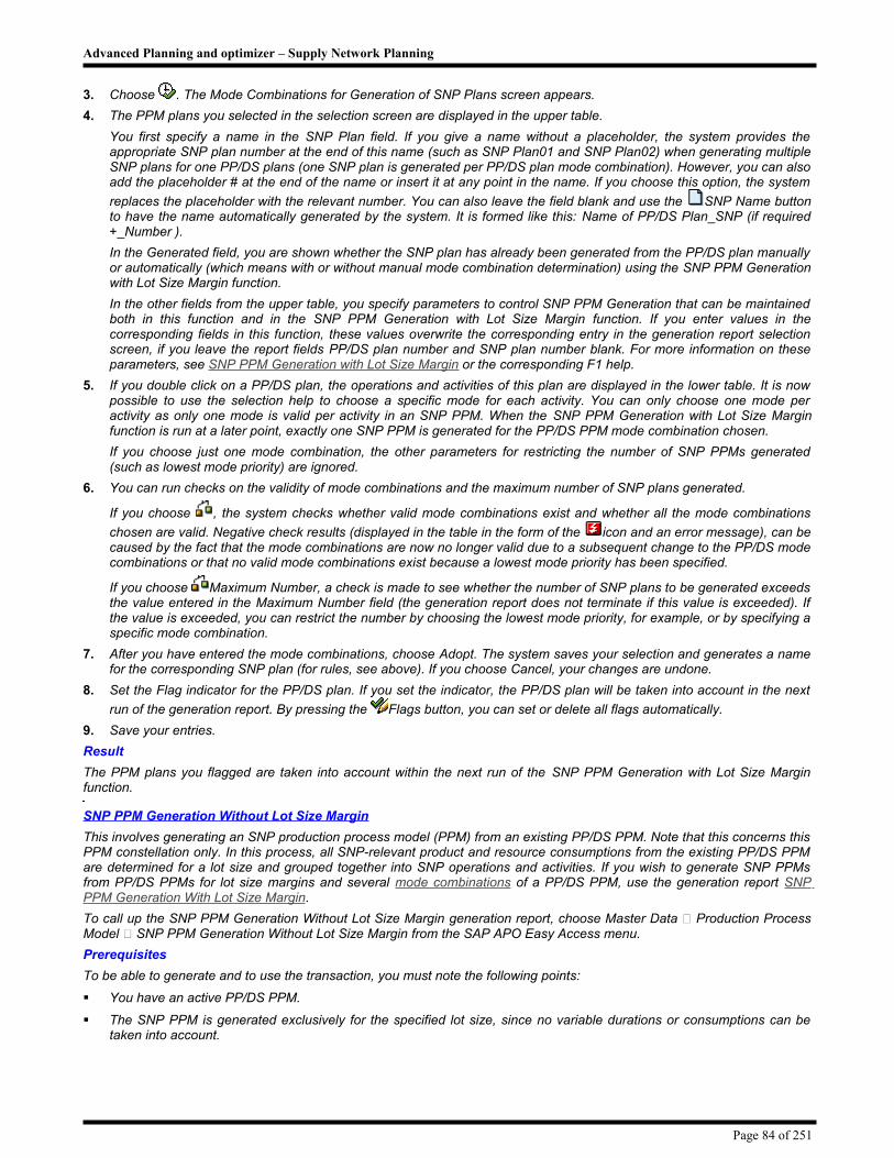
Advanced Planning and optimizer – Supply Network Planning

3. Choose . The Mode Combinations for Generation of SNP Plans screen appears.

4. The PPM plans you selected in the selection screen are displayed in the upper table.

You first specify a name in the SNP Plan field. If you give a name without a placeholder, the system provides the appropriate SNP plan number at the end of this name (such as SNP Plan01 and SNP Plan02) when generating multiple SNP plans for one PP/DS plans (one SNP plan is generated per PP/DS plan mode combination). However, you can also add the placeholder # at the end of the name or insert it at any point in the name. If you choose this option, the system

replaces the placeholder with the relevant number. You can also leave the field blank and use the SNP Name button to have the name automatically generated by the system. It is formed like this: Name of PP/DS Plan_SNP (if required +_Number ).

In the Generated field, you are shown whether the SNP plan has already been generated from the PP/DS plan manually or automatically (which means with or without manual mode combination determination) using the SNP PPM Generation with Lot Size Margin function.

In the other fields from the upper table, you specify parameters to control SNP PPM Generation that can be maintained both in this function and in the SNP PPM Generation with Lot Size Margin function. If you enter values in the corresponding fields in this function, these values overwrite the corresponding entry in the generation report selection screen, if you leave the report fields PP/DS plan number and SNP plan number blank. For more information on these parameters, see SNP PPM Generation with Lot Size Margin or the corresponding F1 help.

5. If you double click on a PP/DS plan, the operations and activities of this plan are displayed in the lower table. It is now possible to use the selection help to choose a specific mode for each activity. You can only choose one mode per activity as only one mode is valid per activity in an SNP PPM. When the SNP PPM Generation with Lot Size Margin function is run at a later point, exactly one SNP PPM is generated for the PP/DS PPM mode combination chosen.

If you choose just one mode combination, the other parameters for restricting the number of SNP PPMs generated (such as lowest mode priority) are ignored.

6. You can run checks on the validity of mode combinations and the maximum number of SNP plans generated.

If you choose , the system checks whether valid mode combinations exist and whether all the mode combinations

chosen are valid. Negative check results (displayed in the table in the form of the icon and an error message), can be caused by the fact that the mode combinations are now no longer valid due to a subsequent change to the PP/DS mode combinations or that no valid mode combinations exist because a lowest mode priority has been specified.

If you choose Maximum Number, a check is made to see whether the number of SNP plans to be generated exceeds the value entered in the Maximum Number field (the generation report does not terminate if this value is exceeded). If the value is exceeded, you can restrict the number by choosing the lowest mode priority, for example, or by specifying a specific mode combination.

7. After you have entered the mode combinations, choose Adopt. The system saves your selection and generates a name for the corresponding SNP plan (for rules, see above). If you choose Cancel, your changes are undone.

8. Set the Flag indicator for the PP/DS plan. If you set the indicator, the PP/DS plan will be taken into account in the next

run of the generation report. By pressing the Flags button, you can set or delete all flags automatically.

9. Save your entries.

Result

The PPM plans you flagged are taken into account within the next run of the SNP PPM Generation with Lot Size Margin function.

SNP PPM Generation Without Lot Size Margin

This involves generating an SNP production process model (PPM) from an existing PP/DS PPM. Note that this concerns this PPM constellation only. In this process, all SNP-relevant product and resource consumptions from the existing PP/DS PPM are determined for a lot size and grouped together into SNP operations and activities. If you wish to generate SNP PPMs from PP/DS PPMs for lot size margins and several mode combinations of a PP/DS PPM, use the generation report SNP PPM Generation With Lot Size Margin.

To call up the SNP PPM Generation Without Lot Size Margin generation report, choose Master Data Production Process Model SNP PPM Generation Without Lot Size Margin from the SAP APO Easy Access menu.

Prerequisites

To be able to generate and to use the transaction, you must note the following points:

You have an active PP/DS PPM.

The SNP PPM is generated exclusively for the specified lot size, since no variable durations or consumptions can be taken into account.

Page 84 of 251

Advanced Planning and optimizer – Supply Network Planning

In the generation process, only single or multi-mixed resources for which the Not SNP Rel. indicator has not been set on the Planning Parameters tab page are taken into account. In addition, only those products for which the SDPrelevance indicator has been activated on the Properties tab page of the product master data are taken into account.

Operations and activities in the SNP PPM do not necessarily match those of the PP/DS PPM from which they were generated. The reason for this is that activities and operations that are contained in non-relevant resources or components are omitted, or are grouped together with other activities in a time bucket because of short duration.

Activities

Using the plan or PPM entered and the lot size, an order is dispatched infinitely to liveCache (without taking into account resource schedules that possibly exist).

Using a time bucket, consumption of the SNP-relevant resources and components can be determined per SNP bucket and grouped together into SNP operations or SNP activities.

Only the valid components and the mode, which is selected automatically via the order explosion, are relevant for generating the SNP PPM.

Consecutive consumptions of the same type are consolidated into one activity, while bucket durations and material consumptions are added together.

If a new component or resource is added to, or removed from a bucket in an SNP PPM, a new activity is generated in this SNP PPM.

If there is a change of primary resource, the system generates a new operation. If several PP/DS activities with different primary resources lie within an SNP bucket, the system checks the resources to see whether the dimensions are the same. The primary resource for the SNP mode is then determined from the PP/DS activity with the highest resource consumption.

Data from the setup matrix is only relevant if the Setup indicator has been set for a setup activity.

Only fixed consumptions and durations can be generated within the SNP plan, because the consumptions arising are determined via a dummy order (fixed lot size). However, if the SNP PPMs generated are also to be valid for lot size margins, the variable portions must likewise be manually calculated out of the fixed portions (see also SNP PPM Generation With Lot Size Margin).

In calculating the bucket consumption, the planned delivery time is also considered. If, for example, a planned delivery time of one day has been specified, the system generates a wait activity for this time. If a PPM is generated in the past, the days up to the generation date are consolidated to form a wait activity.

After generation, you must manually maintain the following texts:

Plan

Product plan assignment

Operation

Activity

This manual maintenance is necessary because the texts cannot be adopted from the PP/DS PPM automatically.

Release of Forecast Data

You can release forecast data to Supply Network Planning (SNP). Depending on your approach, you can choose between the following release methods:

You load data into a Demand Planning planning area and then release the data. For more information, see Release of the Demand Plan to Supply Network Planning.

You release the data directly from an InfoProvider. For more information, see Release from an InfoProvider to SNP.

Release of the Demand Plan to SNP

This process makes the demand plan available to the supply chain planner if the supply chain planner performs Supply Network Planning using liveCache orders. The process also makes the data available in Production Planning and Detailed Scheduling (PP/DS), depending on the horizons that have been maintained for the products involved. (For more information, see the input help for the SNP Prod. Hor. field of the location product master – SNP 2 tab.) In SNP, the supply chain planner can then use the demand plan as a basis for making sourcing, deployment, and transportation decisions. The actual production is then planned in PP/DS.

From a technical point of view, you are copying data from liveCache time series objects to a forecast category in the liveCache orders.

Page 85 of 251

Advanced Planning and optimizer – Supply Network Planning

If Supply Network Planning is performed in liveCache time series, see Copy Management.

In a separate process, the supply chain planner releases the SNP plan to Demand Planning. The data of particular categories in the SNP plan, which has been created or changed by the supply chain planner, is thereby copied to a predefined key figure in a DP planning book. Here, you can perform reporting on the released data and, in particular, compare the original "unconstrained" demand plan with the "constrained" SNP plan. For more information, see Transfer of the SNP Planning Results.

Prerequisites

You have created product master records for your products.

You have created location master records for your locations.

You have set up your supply chain models.

If you are using descriptive characteristics, you need to have previously created a consumption group and assigned it to the relevant products.

If applicable, you have defined the location split for the release to Supply Network Planning. For more information, see

Location Split.

If applicable, you have defined a product split. For more information, see Product Split.

Process Flow

There are two methods for releasing data to SNP:

Online

You can release small amounts of data using an online transaction. For more information, see Releasing the Demand Plan Online.

In the background

You plan mass releases as background jobs that can then be executed when there is little system activity. For more information, see Releasing the Demand Plan with Mass Processing.

Result

Example 1

You create a demand plan in months in Demand Planning. The storage buckets profile contains weeks and months. The technical periods in which the data is stored are as follows:

Time Span of Technical PeriodNumber of Days in Technical Period

Planned Demand Quantity

Monday and Tuesday, February 28 and 29 2 40

Wednesday, March 1 through Sunday, March 5 5 100

Monday, March 6 through Sunday, March 12 7 70

Monday, March 13 through Sunday, March 19 7 70

Monday, March 20 through Sunday, March 26 7 70

Monday, March 27 through Sunday, March 31 5 50

Saturday and Sunday, April 1 and 2 2 20

For the release to Supply Network Planning, you do not specify a planning buckets profile or a daily buckets profile. You specify a release horizon from March 1 through March 31. The system reads the following data and releases it in the same periods to Supply Network Planning. The shipping calendar of the location determines which days are workdays in Supply Network Planning. In this example, all days from Monday through Sunday are workdays.

From-Date To-Date Planned Demand Quantity

March 1 March 5 100

March 6 March 12 70

March 13 March 19 70

March 20 March 26 70

March 27 March 31 50

Page 86 of 251

Advanced Planning and optimizer – Supply Network Planning

Example 2

You create a demand plan in months in Demand Planning. The storage buckets profile contains weeks and months. The technical periods in which the data is stored are as in example 1 above.

For the release to Supply Network Planning, you do not specify a planning buckets profile; you specify a daily buckets profile with 12 days. You specify a release horizon from March 1 through March 31. The system reads the following data:

From-Date To-Date Planned Demand Quantity

March 1 March 5 100

March 6 March 12 70

March 13 March 19 70

March 20 March 26 70

March 27 March 31 50

The following demands are released to Supply Network Planning. The shipping calendar of the location determines which days are workdays in Supply Network Planning. . In this example, all days from Monday through Sunday are workdays.

Period Planned Demand Quantity

March 1 20

March 2 20

March 3 20

March 4 20

March 5 20

March 6 10

March 7 10

March 8 10

March 9 10

March 10 10

March 11 10

March 12 10

March 13 through 19 70

March 20 through 26 70

March 27 through 31 50

Example 3

You create a demand plan in months in Demand Planning.

For the release to Supply Network Planning, you specify a planning buckets profile containing months only but no daily buckets profile. You can specify a planning buckets profile only when releasing data online. You specify a release horizon from March 1 through March 31. The system reads the following data and releases it in the same period to Supply Network Planning.

From-Date To-Date Planned Demand Quantity

March 1 March 31 360

Example 4

You create a demand plan in months in Demand Planning.

For the release to Supply Network Planning, you specify a planning buckets profile containing months only, as well as a daily buckets profile containing 12 days. You can specify a planning buckets profile only when releasing data online. You specify a release horizon from March 1 through March 31. The system reads the following data:

From-Date To-Date Planned Demand Quantity

March 1 March 31 360

The following demands are released to Supply Network Planning. The shipping calendar of the location determines which days are workdays in Supply Network Planning. In this example, all days from Monday through Sunday are workdays.

Period Planned Demand Quantity

Page 87 of 251

Advanced Planning and optimizer – Supply Network Planning

March 1 360/31 = 11.6

March 2 360/31 = 11.6

March 3 360/31 = 11.6

March 4 360/31 = 11.6

March 5 360/31 = 11.6

March 6 360/31 = 11.6

March 7 360/31 = 11.6

March 8 360/31 = 11.6

March 9 360/31 = 11.6

March 10 360/31 = 11.6

March 11 360/31 = 11.6

March 12 360/31 = 11.6

March 13 through 31 360 - (12 * 11.6) = 220.8

The number of decimal places to which the system rounds depends on the number of decimal places defined for the unit of measure in Customizing.

In mass processing, the release horizon is given by the horizon attached to the data view that you specify in the mass processing activity and job.

The Period Split on the SNP2 tab page of the product master record also determines the results of the release to SNP. For more information, see the input help for this field.

If you plan in weeks in Supply Network Planning, the system aggregates the daily quantities into weekly buckets.

If you require a time split other than the ones illustrated above, use functional enhancement APODM017 (transaction CMOD); for example, if you want to create demand quantities in Supply Network Planning on day one and day 15 of every month.

Two Business Add-Ins (BAdIs) are also available for the release function:

Change Data During Release to SNP

Set Requirements Strategy During Release

For more information, see the Implementation Guide (IMG) for Demand Planning under Business Add-Ins → Release to SNP.

Releasing the Demand Plan Online

Use this procedure to release a limited amount of data (a few product / location combinations only) from Demand Planning to Supply Network Planning. Do not use it for mass releases, for example large planning books.

If you try to release too much data with this transaction, memory problems are likely, since the system tries to read all the data simultaneously. For mass processing, use the procedure described in Releasing the Demand Plan with Mass Processing.

Prerequisites

See Release of the Demand Plan to SNP.

Procedure

1. On the SAP Easy Access screen, choose Demand Planning → Planning → Release → Release to Supply Network Planning.

Field Entry

Data Source:

Planning AreaThe planning area from which you want to release the demand plan; that is, the source planning area.

Data Source: Planning Version

The version from which you want to release the demand plan.

Data Source: Key Figure

The key figure that represents the demand plan.

Target: The version to which you want to release the demand plan.

Page 88 of 251

Advanced Planning and optimizer – Supply Network Planning

Planning Version

Target: Category

The order category.

Categories serve to group orders according to different kinds of stocks, goods receipts, goods issues and order types. Enter a category that represents orders or forecasts such as FA or FB. The system creates demand orders with reference to the category in the liveCache order area (also called Order liveCache). The category is determined during the release to SNP as follows:

1. Has a category been entered in the release profile? If yes, this category is used.

2. If no, has a category been set in the definition of the requirements strategy in Customizing? (You define the product’s strategy in the Proposed strategy field on the Demand tab page of the product master record.) If yes, this category is used.

3. If no, the category FA (forecasts) is used.

Add data

If you set this indicator, new order quantities are created in SNP when you release the demand plan from Demand Planning to SNP. The system ignores existing orders in the same SNP version for the same product, location and periods. This means that if you release to SNP twenty times, twenty separate orders are created in SNP.

If you do not set this indicator, existing order quantities in the same SNP version for the same product, location and periods are overwritten.

Set this indicator only in exceptional circumstances.

From-DateA date that defines the beginning of the release horizon.

An entry in this field is compulsory.

To-DateA date that defines the end of the release horizon.

An entry in this field is compulsory.

Planning Buckets Profile

A planning buckets profile that determines how the demand plan is read from liveCache time series for the release to Supply Network Planning.

The use of a planning buckets profile for the release from DP to SNP is optional. If you use a planning buckets profile, the system releases the demand plan in the buckets in which data was planned. The planning buckets profile must be as big as or bigger than the release horizon specified by the From and To dates.

If you do not enter a planning buckets profile, the data is read in technical periods. The storage buckets profile determines what the technical periods are. Technical periods are not visible to the demand planner.

The period split also determines how the demand plan is released to SNP. You set the period split in the product master record (the SNP2 tab).

See also the examples in Release of the Demand Plan to SNP.

Daily Buckets Profile

A planning buckets profile containing days if you wish demand orders to be created in Supply Network Planning in daily buckets.

The use of a daily buckets profile containing days to release the demand plan to SNP is optional. If you use a daily buckets profile, it must contain days only.

During the release, the system works forward in time. For example, if your daily buckets profile contains 40 days, the system releases data to:

The 40 workdays starting on and following the From date if you are releasing the data online.

The first 40 workdays of the planning horizon if you perform the release using mass processing. The planning horizon that is used is the planning horizon of the data view you specify in the mass processing activity and job. Make sure the planning horizon begins in the future, unless you want to release data in the past.

The factory calendar determining which days are workdays is the shipping calendar that you enter in the location master record.

The period split also determines how the demand plan is released to SNP. You set the period split in the product master record (the SNP2 tab).

See also the examples in Release of the Demand Plan to SNP.

Period Split Profile See Time-Based Demand Distribution.

Product Product or range(s) of products for which you wish to release the demand plan.

Page 89 of 251

Advanced Planning and optimizer – Supply Network Planning

Location Location or range(s) of locations for which you wish to release the demand plan.

Extended

If the InfoObjects in the source planning area that represent products and locations are not 9AMATNR and 9ALOCNO, click here to specify the correct InfoObjects.

If you are working with Descriptive Characteristics, you must enter a consumption group. Only then are the descriptive characteristics transferred to order liveCache. You can also specify whether forecasts are generated in order LiveCache for all values of the descriptive characteristics or just for specified values. If you select this option, a button appears with which you can access a selection box.

Results LogTo see the results of the release, check this box. For example, you may wish to do this if the demand plan was created in months but you are releasing to SNP in days. Any errors that occurred during the release are shown in the log.

2. Choose Program → Execute.

Results

See the examples in Release of the Demand Plan to SNP.

Releasing the Demand Plan with Mass Processing

You can use this procedure for releasing any amount of data from Demand Planning to Supply Network Planning in the background. You must use it for large amounts of data, for example whole planning books.

Prerequisites

1. You have created a data view for this task. The use of a separate data view to release a mass demand plan has performance benefits. The data view contains:

A future planning horizon only (no historical horizon, unless you want to release data in the past)

The start date for which data is released is the first day of the planning horizon. The planning horizon is defined in the data view you specify in the planning job.

Only the key figure(s) that you want to release to Supply Network Planning

No actual data rows

2. See also Release of the Demand Plan to SNP.

Procedure

1. Create a release profile.

2. Create an activity.

3. Create a planning job.

4. Schedule the planning job.

5. Review the results in the job log, and take any necessary action.

Release from an Info Provider to SNP

You can use this function to release forecast data from the InfoProvider to Supply Network Planning (SNP). The release takes place directly to SNP. In other words, you do not need to load the forecast data first into a planning area in Demand Planning and thus into the time series liveCache.

Features

You can use the categories for forecast orders (FA, FB, FC, and FD) for the release to SNP. You can release the forecast data from the following objects of the SAP Business Information Warehouse (BW):

InfoCube

VirtualProvider

DataStore Object

MultiProvider

Selection of Data Source

As data sources for the release, you choose an InfoProvider and a planning version and key figure contained in the InfoProvider. If you do not specify any characteristics for product and location under Data Source: Extended Settings, the system uses the characteristics 9AMATNR and 9ALOCNO.

Page 90 of 251

Advanced Planning and optimizer – Supply Network Planning

If you are working with descriptive characteristics for the release, you must specify a consumption group. You must also create at least one planning object structure and a planning area in Demand Planning. This planning area is only required so that you can generate consumption groups. You do not need to create a characteristics combination or store any planning data in liveCache.

Restriction to the Data Source

The standard settings for the grouping condition are product and location, since the release to SNP always takes place at location product level. SNP can only evaluate additional characteristics if you are working with descriptive characteristics. To do so, you must specify a consumption group for the release that contains these characteristics. You must also specify these characteristics in the grouping condition.

If you are working with location splits, you restrict the characteristics exclusively to the location. The system does not evaluate any other characteristics during the release.

Usage of Periodicities

For the release, you can use all periodicities that are available in the InfoProvider. If the selected InfoProvider contains months and weeks, for example, you can select precisely these periodicities, but you cannot select days. For a release of the periodicity month or week or day, the system reads the data from the InfoProvider aggregated to week, month, or day level, and releases the data in the same periodicity to SNP. If you choose more than one periodicity (for example, month and week), the system performs the release with technical periods. If the InfoProvider contains the week and day periodicities and you choose both periodicities for the release, the system also reads the data here from the InfoProvider in technical periods. In this case, the technical periods are identical to the day periodicity.

If you use fiscal year as the periodicity, the selected InfoProvider must only contain one single fiscal year variant.

If you want to release the data aggregated at the level of a periodicity, but this periodicity is not available in the InfoProvider, you can either use a daily buckets profile or a period split profile. For more information about daily buckets profiles, see

Planning Buckets Profile. For information about period split profiles, see Time-Based Demand Distribution.

If you use a period split profile, select exactly one periodicity in the InfoProvider.

Determining the Number of Hits in the InfoProvider

Before the release, you can find out how large the data quantity is that you transfer to SNP. To do so, use Number of Hits in InfoProvider. The system then determines the amount of data for the planning version in the InfoProvider in the specified period.

The system adjusts the specified period automatically to the smallest periodicity available in the InfoProvider. For example, if only the periodicity “month” is available in the InfoProvider, and you enter January 15, 2005 to December 15, 2005 as the period, the system determines the data in the period January 01, 2005 to December 31, 2005.

Activities

If you want to release forecast data from the InfoProvider to SNP, on the SAP Easy Access screen, choose Demand Planning → Planning → Release → Release from InfoProvider to SNP.

Example

In the selected InfoProvider, the data is available in the month and week periodicities. You have chosen both periodicities for the release. The following figure shows how the system determines the technical periods:

The period displayed in the figure comprises the months January to March. A technical period corresponds to the smallest unit of the periodicity you have chosen, that is, a week. January starts in the middle of the first week of the year, whereby the start of the following months can also be within one week. As a result, technical periods, which are shorter than a week, occur at the start and end of the affected months.

Safety Stock Planning

Safety stock planning in Supply Network Planning (SNP) allows you to attain a specific service level by creating safety stock for all intermediate and finished products at various locations throughout the entire supply chain.

Safety stock is used to safeguard stock in the supply chain against uncertain influencing factors. Supply chain planning is susceptible to a number of influencing factors that cannot be predicted with certainty in advance. For example, when forecasting customer demand, the quantity required is usually uncertain. In addition to this, disruptions in production or transportation time fluctuations lead to discrepancies in planned replenishment lead times. To safeguard yourself against such uncertainties when planning, you can take one or more of the following measures:

Page 91 of 251

Advanced Planning and optimizer – Supply Network Planning

Overestimate customer demand

Underestimate production output quantity

Overestimate procurement lead times

Use safety stock

While overestimating customer demand is a Demand Planning tool for safeguarding against forecasting errors, you can model an underestimation of production output quantity and an overestimation of procurement lead times using production process models (PPMs) and transportation lanes.

You have to address the following questions as part of safety stock planning:.

1. At which locations within the supply chain do you want to have safety stock?

2. How much safety stock do you want to hold at a particular location?

Example

With the aid of this simple supply chain, it immediately becomes clear that the question about where to hold safety stock is a highly complex problem due to the variety of possible combinations (calculated as 2 to the power n – in this example, there are already 64 possibilities). Due to this wide range of possibilities, it is advisable to make use of the planner’s experience and allow the planner to simulate selected planning scenarios.

Safety Stock Methods

Since safety stock is usually necessary for products at different locations, you can select a safety stock method in the product master for every location product. The different methods are split into standard and extended methods here.

Standard Methods

The standard methods differ from one another in their observance of time. For these methods, the planner enters the safety stock information directly into the system:

Not time-based (static) Time-based (dynamic)

Safety Stock SB MB

Safety days' supply SZ MZ

Max {Safety stock, safety days’ supply} SM MM

For example, you might want to define safety stock directly as a safety days’ supply or as the maximum of the safety stock and safety days’ supply. With the maximum option, safety stock can be adjusted dynamically to meet the demand flow, and not fall below the defined safety stock. You specify safety stock that is not time-based on the Lot Size tab page in the product master, but define safety stock that is time-based in interactive Supply Network Planning.

Note that for safety stock method MM, the SNP optimizer only considers independent requirements as well as dependent and distributed demands caused by fixed orders, since these demands and the demand locations are already known before the optimization run.

Extended Methods

While the standard methods are based exclusively on the planner’s experience, the proposed safety stock levels of the extended methods are determined by the system based on scientific safety stock planning algorithms. The starting point is a service level that you want to attain through observance of the calculated safety stock. You can define this service level in the Lot Size tab page in the product master. It can be interpreted as follows (based on the business process):

Page 92 of 251

Advanced Planning and optimizer – Supply Network Planning

Shortfall-event-oriented (alpha service level): The service level in percentage means that no shortfall is expected in x percent of the buckets within the planning period.

Shortfall-quantity-oriented (beta service level): The service level in percentage means that x percent of the expected total customer demand can be fulfilled within the planning period.

Example

Bucket 1 2 3 4 5 6 7 8 9 10

Expected demand 100 100 100 100 100 100 100 100 100 100

Shortfall quantity 0 0 0 0 0 10 0 0 0 10

Shortfall event - - - - - x - - - x

Total of shortfall quantities: 20 -> beta service level: 1 – (20 / 1000) = 98%

Total of shortfall events: 2 -> alpha service level: 1 – (2 / 10) = 80%

To decide which service level to use, answer this question: Are the costs for subsequently delivering a shortfall quantity dependent on the shortfall quantity or not? If these costs are not dependent on the shortfall quantity (fixed costs), we recommend that you use an alpha service level; if they are dependent on the shortfall quantity (variable costs), a beta service level would be more appropriate.

The stockholding method used by SNP when planning demands has a major influence on the algorithm for calculating safety stock. The following two different stockholding methods exist:

Reorder cycle method: With this method, the system makes a purchase order decision on a time basis, which means that procurement can only be triggered for all t buckets.

Reorder point method: With this method, the system makes a purchase order decision on the basis of stock, which means that procurement can be triggered if stocks fall below a certain level s (the reorder point).

Stockholding Method

The two service levels result in these four model-supported safety stock methods:

Reorder cycle method Reorder point method

Alpha service level AT AS

Beta service level BT BS

The prerequisite for using this method is that shortfall quantities are delivered subsequently (“back order case” as opposed to “lost sales case”). If this prerequisite is met, the system can calculate the safety stock on any step of the supply chain and for each bucket in the planning period.

Forecast Error Determination

When calculating the safety stock, the system can take into account a forecast error in both demand and procurement. The following key figures form the starting point for the forecast error calculations:

Demand Procurement

Planned demand quantity key figure Planned replenishment lead time key figure

Realized demand quantity key figure Realized replenishment lead time key figure

Page 93 of 251

Advanced Planning and optimizer – Supply Network Planning

The system calculates the forecast error by determining the planned actual deviation of the relevant key figures. The standard deviation of the planned actual deviations is interpreted as the forecast error. A forecast error is thus determined from the historical data and the future forecast is based on this forecast error. To more accurately support the future forecast, it is a good idea to interpret this forecast error as a relative forecast error, so that instead of keeping the forecast error itself, you keep the relationship between forecast error and forecast (variation coefficient). This is clarified in the following example:

Example

Mean value of the planned demand quantity: 100

Standard deviation of the planned actual deviations: 10

Bucket 1 2 3 4 5

Demand Forecast 100 1000 1000 100 100

Forecast error if the standard deviation is constant 10 10 10 10 10

Forecast error if the variation coefficient is constant 10 100 100 10 10

If the forecast error is not dependent on the forecast, an incremental forecast unexpectedly causes the safety stock to fall because the forecast error decreases in relation to the forecast. For this reason, it is more advisable to use relative forecast errors in a dynamic environment than constant forecast errors.

If there is a forecast error in procurement (a replenishment lead time forecast error), the demand forecast error is adjusted based on the assumption that the two forecast errors are independent of each other.

You can also enter the demand forecast error and replenishment lead time forecast error directly in the location product master. We recommend that you do this in the following circumstances:

If there is no historical data (because the product is new for instance)

If the amount of historical data is so small that it is impossible to calculate a statistically relevant forecast error

If the forecast error can be considered constant

In the safety stock planning profile, you can specify if the system is to calculate the forecast error during extended safety stock planning from the historical data or from the location product master data.

Modifying the Parameters

Multilevel safety stock planning is a very complex issue for any supply chain structure. It is therefore a good idea to implement high-performance heuristics. Algorithms are thus the focus of attention for single-level, non-time-based safety stock planning that is then incorporated within a multilevel, time-based supply chain planning by adjusting the input parameters.

This makes it necessary for the system to adjust the forecast and forecast error for demand and procurement.

For demand, the system first determines all the location products supplied by the safety stock location product. It then projects all the forecasts and forecast errors onto the safety stock location product (considering all the quantity and time relationships) to calculate the safety stock.

For procurement, the system first determines all the location products that are to supply the safety stock location product. It will do this until it finds a safety stock location product, or until it finds external supply for the supply chain. It then determines the critical supply path by calculating the maximum replenishment lead time. All forecasts and forecast errors along this critical path are then projected onto the safety stock location product for safety stock planning.

See also:

Standard Safety Stock Planning, Extended Safety Stock Planning, Master Data Setup for Safety Stock Planning

Standard Safety Stock Planning

You use standard safety stock planning in Supply Network Planning (SNP) to build up safety stock for location products according to values that match past experience. You can define these values as time-independent in the location product master data or time-dependent in interactive SNP planning. When doing so, you can choose from six different safety stock methods with which you define the safety stock directly using the safety days’ supply or as a maximum of safety stock and safety days’ supply.

The values you have defined are then considered during heuristic or optimization-based SNP planning.

Prerequisites

You have defined the specific master data for standard safety stock planning. For more information see Master Data Setup for Safety Stock Planning.

Page 94 of 251

Advanced Planning and optimizer – Supply Network Planning

If you wish to use safety stock methods MZ, MB, or MM, you have to use standard SNP planning area 9ASNP05 and standard planning book 9ASNP_SSP (or a planning area and planning book based on these) that contain the following key figures: 9ASAFETY – Safety Stock (Planned) and 9ASVTTY – Safety Days’ Supply.

Note that for safety stock method MM, the SNP optimizer only considers independent demands as well as dependent and distributed demands caused by fixed orders, since these demands and the demand locations are already known before the optimization run.

Activities

The safety stock values you defined are shown in interactive SNP planning and the system considers them during the SNP planning runs.

Extended Safety Stock Planning

Extended safety stock planning in Supply Network Planning (SNP) automatically calculates the safety stock using data that you specified as mandatory in the system. This includes, for example, a service level that you want to attain through observance of the calculated safety stock. You also specify the current demand forecast and the historical data using the demand forecast and the replenishment lead time (RLT) as key figures. The system uses the historical data to calculate the forecast error for the demand forecast and the RLT.

Prerequisites

You have assessed your supply chain and determined at which stages you want to plan safety stock.

You have determined the special master data for safety stock planning next to the basic SNP planning master data (including quota arrangements). This includes, for example, the service level and the safety stock methods in the location product master data. For more information see Master Data Setup for Safety Stock Planning.

You have created a safety stock planning profile (SFT planning profile). In this profile you can, for example, determine how the system calculates the forecast error (from historical or master data), and specify the demand type (regular or sporadic). For more information, see Safety Stock Planning Profile.

Features

The system considers the following factors when calculating the safety stock:

Demand forecast and demand forecast error

Replenishment lead time (RLT) and RLT forecast error

Service level

Safety stock method

Demand type

The reorder point method that you determined in the location product master data does not influence safety stock planning.

The system determines these factors as follows:

Demand Forecast Determination

The forecasted demand for a product at a location is the sum of the independent and dependent demands at the location and all downstream locations. You specify the independent demands in the system as a key figure for the demand forecast. The system determines the dependent demands using transportation lanes and production process models (PPM) or production data structures (PDS). The system also takes into account inbound quota arrangements.

The system determines the demands forecast error from the historical data or location product master data that you specified as mandatory (settings in SFT planning profile).

Replenishment Lead Time Determination

The RLT for a product at a location is the total time for the in-house production or the external procurement of a product (including its components). The system determines the RLT using the supply chain model or from location product master data (settings in SFT planning profile).

If the system determines the RLT using the supply chain model, it adds up the respective production times, good issue processing times, transportation times, goods receipt processing times, and planned delivery times. If there are alternative procurement options, the system always considers the option that takes the longest time. The system does not consider restrictions on capacity size, lot size, or warehouse stock. Procurement from upstream safety stock is not restricted.

The system determines the RLT forecast error from the historical data or location product master data that you specified as mandatory (settings in SFT planning profile).

Service Level Determination and Safety Stock Method Determination

Page 95 of 251

Advanced Planning and optimizer – Supply Network Planning

The system determines the service level and the safety stock method from the location product master data (Lot Size tab page). With the safety stock method you determine the combination of service level and order policy that the system is to consider.

During the reorder cycle methods AT and BT the system interprets the target days’ supply from the location product master data as an order cycle.

During the reorder point method BS the system uses the target days’ supply from the location product master data to calculate the purchase order quantity.

During the reorder point methods AS and BS the system accepts a monitoring interval (period of time between successive reviews of the warehouse stock) from one period.

Demand Type Determination

You can use safety stock planning both for products with regular demand and also for products with sporadic demand. For the former, the formulas used assume normal distribution, for the latter they use gamma distribution.

The system determines the demand type from the settings you made in the SFT planning profile. You can determine whether it is regular or sporadic demand, or whether the system is to automatically determine the demand type using historical data.

Activities

On the SAP Easy Access screen, choose Advanced Planning and Optimization →Supply Network Planning → Planning → Safety Stock Planning. On the Safety Stock Planning screen, you then enter the data described below:

Section Input data

Planning Data

In this section you then specify the planning area where the planning objects and key figures are. You can use, for example, the SNP standard planning area 9ASNP05 (or a planning area based on it) that contains the key figures 9ADFCST, forecasting, and 9ASAFETY, safety stock (planned).

You can also specify the key figure for the demand forecast, based on which the system calculates the safety stock (for example, 9ADFCST). You can also specify the key figure in which the system saves the safety stock (for example, 9ASAFETY) and the SFT planning profile the system uses.

Object Selection

In this section you specify the location products for extended safety stock planning. The system plans the safety stock for those location products for which you have determined an extended safety stock method in the master data.

Historical Data

In this section you specify the key figures for the demand forecast historical data which the system uses to calculate the forecast error. You can, however, determine the forecast error in the location product master data yourself.

Application Log

In this section you specify how the system creates the application log (level of detail, immediate display, length of storage).

You can display the calculated safety stock as a key figure in interactive Supply Network Planning and, if required, manually change it or copy it into another planning version. You can also use the calculated safety stock in Production Planning & Detailed Scheduling (PP/DS) and Capable-to-Match (CTM).

Safety Stock Planning Profile

This profile contains settings for extended safety stock planning in Supply Network Planning (SNP).

If you execute extended safety stock planning in SNP, you must specify a safety stock planning profile (SFT planning profile). In this profile you determine settings for safety stock planning that rarely have to be changed. This includes, for example, how the system calculates the replenishment lead time (RLT) forecast and the RLT forecast error.

Structure

The profile consists of the following sections:

Profile

In this section you give the profile a name and a description.

Demand

In this section you determine how the system calculates the demand forecast error (from historical data or location product master data). You can also correct the level of the demand forecast and the demand forecast error up or down.

Replenishment Lead Time

In this section you determine how the system calculates the replenishment lead time forecast (from the supply chain structure or location product master data).

Page 96 of 251

Advanced Planning and optimizer – Supply Network Planning

You also determine how the system calculates the forecast error (from historical data or location product master data). You can also correct the level of the RLT forecast and the RLT forecast error up or down.

Safety Stock Calculation

In this section you determine the requirements category that the extended safety stock planning is to use as the basis for its calculation (regularly, sporadically, or automatically).

You can also specify that the system takes into account the location product fixed lot size, defined in the location product master data, while calculating the procurement qualities.

Further settings

In this section you determine the block size with which the extended safety stock planning saves the result in the liveCache. You can also specify that the system checks the supply chain in cycles to avoid endless loops during the planning.

If you want to carry out aggregated safety stock planning, you can specify the level at which the system is to consider the sources of supply: sub location product level, header location product level, or at both levels (default value).

When you specify a new profile, the system offers you default values. You can also use the SNP standard profile SAPDEFAULT that also contains default values.

Supply Network Planning Run

You can use any of the following planning methods to perform the planning run in Supply Network Planning (SNP):

Optimization-Based Planning

Heuristic-Based Planning

Supply and Demand Propagation

You can run optimization-based and heuristic-based planning interactively from the interactive planning desktop in Supply Network Planning or you can run them in the background. You run supply and demand propagation in a dedicated planning book in interactive Supply Network Planning.

Based on these planning methods, SNP supports special planning processes, such as:

Aggregated Planning

Planning with Aggregated Resources

Product Interchangeability

Procurement Scheduling Agreement in Heuristic-Based SNP Planning

Subcontracting with Source Location in SNP

Subcontracting with Third-Party Provision of Components in SNP

Direct Delivery from Production Plant to Customer

For detailed information about the individual planning methods and processes, see the related sections of this documentation.

Your individual planning environment influences which planning method would be the most suitable for your requirements. For a comparison of the heuristic and optimization planning methods with Capable-to-Match (see below), see Comparison of the Planning Methods.

See also

Capable-to-Match planning (CTM) is an alternative to the optimization-based or heuristic-based planning methods from

Supply Network Planning. For more information, see the Multilevel Supply and Demand Matching section of the SAP APO documentation.

Comparison of the Planning Methods

Optimization-based planning and heuristic-based planning are the two main planning methods of Supply Network Planning

(SNP). This topic compares these two planning methods with the Capable-to-Match (CTM) planning method.

We recommend that you use optimization-based planning or CTM planning if one of the following conditions applies to you:

Your business environment is subject to strict constraints (for example, you must take into account production capacities, transportation capacities, storage capacities, and/or handling capacities)

You have alternative production locations and sources of supply (locations, production process models, and external procurement relationships)

You can decide between early production and late production

Page 97 of 251

Advanced Planning and optimizer – Supply Network Planning

You share resources, meaning that multiple products are produced simultaneously on the one resource

We recommend that you use heuristic-based planning or CTM planning if any of the following conditions apply:

You wish to plan on an infinite basis (meaning that you do not wish to consider capacities) for the medium to long-term horizon (heuristic).

You wish to take into account predefined quota arrangements; for sources of supply, for instance (heuristic or CTM).

You wish to plan or fulfill demands on the basis of priorities (CTM).

The following table describes the main features of each planning method:

Business Environment

AreaHeuristic and Capacity Leveling

Capable-to-Match Optimizer

Business Objective To create a feasible plan

with few bottleneck resources

To create a feasible plan by fulfilling the highest priority demand first

To create a feasible plan with minimum costs

To maximize profits

Demand Type Not relevant Prioritized demand and

demand-specific supply strategies

Demand can be aggregated for three demand classes or by customer locations

Capacity

Heuristic run: Based on the assumption that capacity is infinite (infinite capacity planning)

Capacity leveling: This is a step following on from the heuristic run to level capacities

Finite capacity planning (taking capacity constraints into account) or a simulation of infinite planning

Finite or infinite capacity planning

Planning Approach Bucketed (period-based) planning

Bucketed or continuous planning

Bucketed planning

Constraints and Business Scenarios

AreaHeuristic and Capacity Leveling

Capable-to-Match Optimizer

Resources

Production

Transportation

Handling (heuristic only)

Production

Production

Transportation

Storage

Handling

Target Stock Levels

Flexible definitions for the heuristic but capacity levelling does not consider the target stock level method specified

Can use absolute target stock levels or target days’ supply for planning

Can use absolute target stock levels or target days’ supply for planning. The optimizer calculates the target days’ supply before the actual optimization run

Lot Sizes

Considers lot sizes for production, transportation, and procurement

Considers lot sizes for production, transportation, and procurement

Considers lot sizes for production and transportation

Considers cross-period lot sizes for production

Transportation lot sizes have to be used to map lot sizes for procurement

Source Determination (sourcing)

Based on quota arrangements and

Based on costs (PPM/PDS and transportation),

Cost-based sourcing decisions

Page 98 of 251

Advanced Planning and optimizer – Supply Network Planning

AreaHeuristic and Capacity Leveling

Capable-to-Match Optimizer

priorities

priority, or quota arrangements (quota arrangement does not split orders unless necessary to fulfill demands on time)

Does not take quota arrangements into account but can be used to modify quota arrangements

Time-Based Production Parameters Considered Considered Considered

Material Constraints

Material staging is not a constraint. A backlog is created for externally planned products

Considers material constraints; external products are not planned and do not represent a material constraint

Can consider material constraints for externally planned products or by setting a high procurement cost for procured products

Supply Categorization Not supported You can define supply

categories Not supported

Supersession and Discontinuation of Products

1:1 - Supports supersession (supersession chains and form-fit-function classes)

1:1 - Supports supersession (forward interchangeable supersession chains only)

1:1 - Supports supersession (supersession chains and form-fit-function classes)

Hierarchical Planning Supports aggregation

planning and disaggregation

Does not support aggregation based on hierarchies but you can choose to aggregate demands and supply on a time basis or by order types for product

Supports aggregation planning and disaggregation

Maximum Stock Levels by Product Not considered Not considered

Considered as a constraint

Push Distribution Stock to Downstream Locations

Not supported (but is supported by deployment)

Not supported (but is supported by deployment and by supply distribution in CTM)

Can be controlled using storage costs

Minimum Resource Utilization Not supported Not supported

You can define a minimum available capacity for a resource and assign costs for falling below this minimum level (this only applies to production resources)

Resource Capacity

Does not make a distinction between standard and extended capacity

Does not make a distinction between standard and extended capacity

Can make a distinction between standard and extended capacity

Demand Prioritization Capacity leveling does

not recognize demand priorities

Demand can be sorted by different sort criteria

Demand can be aggregated for three demand classes or by customer locations

Shelf life Not considered Not considered

Can consider shelf life constraints in a restricted way (see SAP note 579556)

Batches are not recognized

Page 99 of 251

Advanced Planning and optimizer – Supply Network Planning

AreaHeuristic and Capacity Leveling

Capable-to-Match Optimizer

Subcontracting

Supported (the subcontractor has to be modeled as a location)

Supported (the subcontractor has to be modeled as a location)

Supported (the subcontractor has to be modeled as a location)

Scheduling Agreement Processing Supported Not supported Not supported

Configuration

AreaHeuristic and Capacity Leveling

Capable-to-Match Optimizer

Relevant Master Data

Locations

Products

Resources (single-mixed, multi-mixed, and bucket resources)

PPMs and PDSs (SNP)

Transportation lanes

Locations

Products

Resources (single-mixed or multi-mixed, and bucket resources)

PPMs and PDSs (SNP and PP/DS, but some restrictions)

Transportation lanes

CTM profile (supply profiles, demand profiles, and so on)

Locations

Products

Resources (single-mixed or multi-mixed, and bucket resources)

PPMs and PDSs (SNP)

Transportation lanes

SNP optimizer profile

Optimizer costs

Flexibility of Algorithm Macros can be used to

modify heuristic values that are entered

You can modify aspects of the calculation by changing profile settings and maintaining parameters

Has a user function for modifying the optimizer input log

Macros can be used to modify optimizer values that are entered

Average Effort Minimal

Medium to large, depending on the complexity of the supply chain

Medium to large, depending on the complexity of the supply chain

Cost fine-tuning is the major effort

Current Application Capacity leveling only

considers one resource at a time

After the parameters have been configured, CTM can be run automatically

After costs are fine-tuned, the optimizer can be run automatically

Comprehensibility Transparent results

Transparent results based on priorities. The analysis complexity is governed by the supply chain complexity

Order tracking by pegging

Graphical representation of results

Requires some understanding of cost tradeoffs

Cost summaries are available after the optimization run

Integration with PP/DS Bucketed plans need

to be converted into continuous plans

Bucketed plans need to be converted into continuous plans

Continuous plans can be created

Bucketed plans need to be converted into continuous plans

Recognizes material flow, capacity consumption, and setup statuses from PP/DS

Net Change Planning Supported Supported - with options for dynamic and fixed

Have to replan all

Page 100 of 251

Advanced Planning and optimizer – Supply Network Planning

pegging

demands

Can use the SNP optimization bound profile to restrict replanning

Optimization-Based Planning

The SNP optimizer offers cost-based planning. This means that it searches through all feasible plans in an attempt to find the most cost-effective (in terms of total costs). Total costs refers to the following:

Production, procurement, storage, and transportation costs

Costs for increasing the production capacity, storage capacity, transportation capacity, and handling capacity

Costs for violating (falling below) the safety stock level

Costs for late delivery

Stock out costs

You use the SNP cost profile to fine-tune the relative importance of different cost types.

In the optimizer view, a plan is feasible when it satisfies all the Supply Chain Model constraints that you set in the SNP optimizer profile. A feasible solution might involve due date or safety stock constraint violations. Due dates and safety stocks are Soft Constraints (constraints to which you assign violation costs). The optimizer only proposes a plan that will violate soft constraints if, according to the costs specified in the system, it is the most cost-effective plan.

The optimizer makes sourcing decisions within optimization-based planning. This means that it uses costs as a basis for deciding the following:

Which products are to be produced, transported, procured, stored, and delivered and in which quantities (product mix)

Which resources and which production process models (PPMs) or production data structures (PDSs) to use (technology mix)

The dates and times for production, transportation, procurement, storage, and delivery

The locations for production, procurement, storage, delivery, and the source and destination locations for transportation

Since you can enter PPMs or PDSs with fixed resource consumption in master data, you can also include setup operations in Supply Network Planning. Therefore, you can also use the SNP optimizer for lot size planning. The optimizer also supports cross-period lot size planning where orders are grouped into large lots due to high set up costs.

The optimizer uses the linear programming method to take account of all planning-problem-related factors simultaneously within one optimal solution. As more constraints are activated, the optimization problem becomes more complex, which usually increases the time required to solve the problem. As a rule, you should run optimization as a background job.

The optimizer makes a distinction between continuous linear optimization problems and discrete optimization problems.

Linear Optimization

You can choose one of the three following methods in the SNP optimizer profile to solve continuous linear optimization problems:

Primal simplex method

Dual simplex method

Interior point method

All three methods arrive at an optimal solution. Runtime could be the main influencing factor when deciding which of these methods to use. However, there is no general rule for selecting the best method for a given problem (apart from to test each method individually). A good way of assessing the application is to do a benchmarking based on a test scenario. This is because the optimal choice of method depends more on the structure of the supply chain and less on the input data. Therefore, in a productive environment, daily benchmarking is not necessary.

Discrete Optimization

A problem is not continuous (and is therefore discrete) in Supply Network Planning, when the model contains:

Discrete (integer-value) lot sizes for transportation or PPMs/PDSs

Discrete means of transport

Discrete increase of production capacity

Minimum lot sizes for transportation or PPMs/PDSs

Piecewise linear cost functions for transportation, production, or procurement

Page 101 of 251

Advanced Planning and optimizer – Supply Network Planning

Fixed PPM/PDS resource consumption

Fixed PPM/PDS material consumption

Cross-period lot size planning

If you want the optimizer to consider any of the above constraints, you must use one of the discrete optimization methods from the SNP optimizer profile.

The piecewise linear cost function that you can define in master data makes a distinction between the convex cost function (cost per unit increases for higher volumes; for modelling overtime or night shifts for instance) and the concave cost function (cost per unit decreases for higher volumes; for modelling freight rates for instance).

Convex cost functions do not complicate the planning problem and can be solved efficiently. However, they can also be modelled using alternative modes without using piecewise linear cost functions.

Mode 1 with $50 per unit and a limited capacity of eight models

Mode 2 with $100 per unit and a limited capacity of six models

Convex functions of labour cost per day, assuming eight normal working hours and a maximum of six hours of overtime paid at double time

In contrast, concave piecewise linear cost functions cannot be solved by an LP solver but only by using discretization methods (mixed integer linear programming). If piecewise linear functions are modelled but the optimizer is run without discretization or the discretization horizon is smaller than the planning horizon, the optimizer takes into account the linear cost function defined in addition to the piecewise linear cost function.

The discrete optimization method cannot be used with strict prioritization (see below).

Using the discrete optimization method can significantly increase runtime requirements. Note that Supply Network Planning is a medium-term planning function and its focus should not be on solving integer problems (that is, using the discrete optimization method).

Prioritization

The optimizer can differentiate between the priority of sales orders and forecast demand. With strict prioritization, sales orders always have priority 1, the corrected demand forecast priority 5, and the demand forecast priority 6. Within every priority class, the system uses all available cost information to determine the final solution. When cost-based prioritization is used, the optimizer uses penalty cost information from the product master data (the SNP1 tab page) to determine the optimal solution.

Decomposition

You can use the decomposition methods, defined in the SNP optimizer profile, to reduce runtime and memory requirements for optimization. Decomposition may also represent the only way for the optimizer to find a feasible solution in the event of large discrete problems. For more information, see Decomposition.

Aggregated Planning - Vertical

To reduce the size of the model to be optimized, the optimizer can restrict planning to location product group level (assuming you have defined the demands at the lower level). Plans are distributed to lower level products based on demand for the lower level products. To plan at product group level, you must define hierarchies for products and locations in the hierarchy master. This data is used to generate the location product hierarchy. You also must define the PPMs or PDSs for the product groups and create the PPM or PDS hierarchy in the hierarchy master. In the SNP optimizer profile, if you set the Aggregated Planning - Vertical indicator, the products are automatically aggregated to the relevant groups for planning and after planning is complete, they are disaggregated again.

Aggregated Planning - Horizontal

This function allows you to plan a subset of your supply chain. You can limit the products or locations to be taken into account during the optimization run. For example, if optimization is only run to plant level but forecasts are at customer level, the optimizer can sum (aggregate) the demands to plant level and use this value during the optimization run. The transportation times, for example, from the plant to the distribution center and to the customer, as well as the duration of the PPMs or PDSs, are also taken into account.

Incremental Optimization

Incremental optimization is the name given to optimization-based planning that is run for only part of the model or on the basis of an already existing plan. The plan might be infeasible with this type of optimization since the optimizer cannot plan receipts for shortages that are the result of fixed orders from previous planning runs. It is also possible that the optimizer will ignore input products (and associated stock) that are defined in PPMs / PDSs or products that are available for procurement at a source location using a transportation lane (source location products).

To prevent this, you can specify in the SNP optimizer profile that the optimizer is to take into account the stocks of non-selected input products or source locations products. You can also specify that the dependent demand and distribution demand of fixed orders is to be treated as an independent requirement, meaning that the optimizer will permit shortages subject to the calculation of penalty costs for not delivering. You define penalty costs for not delivering for customer demand,

Page 102 of 251

Advanced Planning and optimizer – Supply Network Planning

the demand forecast, and corrected demand forecast in the product master data. You can also set that the optimizer is to consider the dependent demand and distribution demand of fixed orders, and the stocks of non-selected input products or source location products as a pseudo-hard constraint. This means that shortages are possible but are subject to the calculation of infinitely high penalty costs that are internally defined in the optimizer. Setting this ensures that the optimizer will only permit shortages if it cannot find any other feasible solution.

Process Flow

1. You run the optimizer.

2. You run deployment.

3. You run the TLB.

The Optimization Run

Note: The optimizer plans all distribution demands for all locations in the distribution network before exploding the BOM and processing dependent demand at the production locations.

Factors Considered During the Run

Valid transportation lanes

Lead times

Transportation capacity

Transportation costs

Handling capacity

Handling costs

Production capacity

Production costs

Storage capacity

Storage costs

Time stream (location master data)

Lot size (minimum, maximum, and rounding value)

Scrap

Application Examples for the SNP Optimizer

Below is a list of examples showing where you can use the SNP optimizer within production planning and distribution resource planning and what you should keep in mind:

Page 103 of 251

Advanced Planning and optimizer – Supply Network Planning

1. Finite Capacity Planning

It is particularly advisable to use the SNP optimizer to plan capacities as finite if you have limited business resource capacities and these limited capacities have an impact on your production planning and distribution resource planning. By already planning capacities as finite in Supply Network Planning (SNP), you can take capacities into account and make it easier for the subsequent detailed scheduling (such as SAP APO Production Planning and Detailed Scheduling, PP/DS) to create feasible plans.

Furthermore, by using the SNP optimizer to plan finite capacities, you can include a possible extension of your capacities into your plan, subject to the calculation of additional costs.

You can use the SNP optimizer to plan the following resource categories and types as finite:

Resource categories:

Production resources

Transportation resources

Handling resources

Storage resources

Resource types:

Single-mixed and multi-mixed resources

Bucket resources

Transportation resources

Integration

The SNP optimizer takes into account the net available capacity only, meaning that it checks whether the capacity available in SNP is already being used by other system application areas (PP/DS, deployment, or the Transport Load Builder, for example) or by fixed SNP orders.

For single-mixed and multi-mixed resources, the SNP optimizer subtracts the capacity consumed by PP/DS, for instance, from the capacity available in SNP. If the capacity consumed by PP/DS exceeds the aggregated available capacity in a bucket in SNP, the optimizer assumes that there is an available capacity of 0 in the corresponding bucket and plans no further capacity consumption in this bucket.

Prerequisites

The prerequisites for finite capacity planning are the same as those for general optimization-based planning:

Planning Area Administration

Master Data Setup for the Optimizer

Model/Version Creation

Supply Chain Model Setup

Release of the Demand Plan to SNP

Features of Finite Capacity Planning

General Information

Generally, the SNP optimizer takes into account all model constraints simultaneously. This means that the optimizer takes into account the available capacity of all resources at the same time. Thus, during multilevel production, for example, all the manufacturing levels are incorporated simultaneously into planning.

In the SNP optimizer profile, you can set which capacity constraints (production capacity, transportation capacity, handling capacity, or storage capacity) you want the optimizer to take into account.

The optimizer determines the available capacity based on the defined factory calendar, meaning that it only uses days defined as workdays to determine the bucket capacity.

You can define multiple capacity variants for resources and label these as the minimum, normal, or maximum available capacity. Thus, you can let the optimizer decide to increase capacity or fall below the minimum capacity subject to the calculation of additional costs. Since the optimizer generally chooses the solution with the lowest costs, it will only increase capacity or fall below the minimum if this course of action is the most cost-effective total solution despite the additional costs.

You define the costs for the capacity variants with minimum, normal, or maximum capacity in the quantities/rate definition or the capacity profile of the resource master data. To set the status indicator, go to the resource initial screen

and choose: Current Settings -> Capacity Variants (see also, Master Data Setup for the Optimizer).

Page 104 of 251

Advanced Planning and optimizer – Supply Network Planning

Note that the optimizer takes into account the minimum available capacity and the costs you defined for a capacity variant with the status Normal Capacity only for production resources.

Production Resources

Capacity Consumption

The SNP optimizer takes into account the capacity consumption of a production resource, which you define in the production process model (PPM) mode. One PPM can load several resources and one resource can be loaded by several PPMs. The duration of an SNP PPM (that is, the sum of the duration of all PPM activities) is fixed. It has no influence on resource consumption and instead is used only for scheduling within the PPM.

The resource consumption defined per activity is distributed evenly over the length of the activities. This means that the optimizer ignores the consumption type defined for the activity and always assumes that consumption is continuous (consumption type C).

If you use the linear optimization method, the optimizer only takes into account the variable resource consumption defined in the PPM. If you want the optimizer to also take into account fixed resource consumption, you have to choose discrete optimization in the SNP optimizer profile and define a discretization horizon for the Fixed Material and Resource Consumption. This is necessary if, for instance, you want to use fixed resource consumption to model setup times during lot size planning with the SNP optimizer (see also, Lot Size Planning).

Note that the optimizer ignores the fixed resource consumption defined in the PPM if you choose the linear optimization method in the SNP optimizer profile. However, fixed resource consumption is taken into account if orders are created in liveCache during planning. This can cause a resource overload to be displayed in the capacity view of interactive Supply Network Planning. Therefore, if you want the optimizer to take into account the fixed resource consumption, choose discrete optimization or do not define a fixed resource consumption in the PPM.

If you are running an integrated SNP and PP/DS planning and set the Lot Size Planning: Not Cross-Period indicator in the SNP optimizer profile (the Integration tab page), fixed resource consumption is not taken into account when creating SNP orders in liveCache if there is already an existing PP/DS order for the associated PP/DS PPM (see also the F1 help at the indicator). This also applies for Cross-Period Lot Size Planning if you set the accompanying Cross-Period Lot Size Planning indicator.

The optimizer also takes into account time-based resource consumption that you defined in the PPM. You can use time-based consumption to model varying consumption levels over the course of the bucket. For example, you could include the following information in your plan: A machine consumes more lubricant at the beginning of production than it does towards the end.

Available Capacity

For the maximum available capacity variant of production resources (see above), you can define that the optimizer is permitted to either increase the capacity by this variant’s entire available capacity (an entire layer, for example), or not increase it at all. In this instance, the optimizer either takes into account the entire costs of the increase or no costs at all. In the SNP optimizer profile, choose the discrete optimization method and define a discretization horizon in the Discrete Production Capacity Increase field.

Capacity Costs

You can also define time-based costs for increasing the capacity of production resources. For a daily planning buckets profile, you can define that the increase costs more on a Monday than it does on a Tuesday, for example.

You also have the option of defining costs for the normal capacity variant (standard capacity) for production resources. You can specify these costs (also on a time basis) per capacity unit and bucket. The costs incurred are proportional to the resource usage.

If you wish to define a minimum available capacity (see the General Information section), you have to define costs for falling below it. You can also specify these costs for each capacity unit and bucket. The costs incurred are proportional to the amount fallen below the minimum available capacity.

Constraints

Since you can only create one mode per activity in the SNP PPM, you cannot define any alternative resources for a production activity. To define alternative resources, you must create one PPM per mode combination. You can use

the SNP PPM Generation With Lot Size Margin function to generate SNP PPMs automatically for multiple PP/DS PPM mode combinations.

Transportation Resources

Capacity Consumption

The SNP optimizer only takes into account the means of transport’s variable capacity consumption (per day) that you specified in the Consumption field of the Product-Specific Means of Transport section. You specify consumption for the product that is defined in this section. Consumption is dependent on the transportation duration. If the transportation duration is 0, no resource consumption exists.

Page 105 of 251

Advanced Planning and optimizer – Supply Network Planning

If you do not enter a value in the Consumption field or do not define any data for the Product-Specific Means of Transport, the optimizer calculates consumption using the conversion factor for units of measure that you specified on the Units of Measure tab page in product master data.

Available Capacity

You can assign transportation resources to multiple transportation lanes and so limit the transportation capacity on these transportation lanes. To do this, specify a transportation resource in the Resource field of the Means of Transport section in the transportation lane.

In the SNP optimizer profile, you can set that you want the available means of transport to be treated as discrete (in non-divisible integer numbers). If you do this, the means of transport is treated as discrete for each transportation lane. You define the capacity of the means of transport in the Transp.Res.Size field of the resource master data.

You can use this option to model the means of transport that are available in your company (a truck, for example). However, if you commission external transportation service providers, considering means of transport as discrete is not relevant for you.

Capacity Costs

The transportation costs considered by the optimizer consist of the product-specific transportation costs (that is, the transportation costs you entered in the Product-Specific Means of Transport section in the transportation lane) and the transportation costs for the means of transport (that is, the transportation costs entered in the Means of Transport section). The means of transport costs are dependent on the transportation resource consumption of all the products transported on the transportation lane and the distance that was defined for the transportation lane between the start location and destination location.

You can define the means of transport costs either as costs per transportation resource unit or as costs per means of transport. For the costs per transportation resource unit, you do not define a size for the transportation resource. However, for the costs per means of transport, you do define a size (5 t, for example) and set the Integral Means of Transport indicator in the SNP optimizer profile, if required (when activating this indicator, you must also choose the discrete optimization method in the SNP optimizer profile).

If, for instance, you want to model discount scales for the costs per transportation resource unit option, you can use cost functions. Cost functions are most appropriate when you are working together with external transportation service providers.

Handling Resources

Capacity Consumption

You can assign handling units to a location (on the Resources tab page) as handling-in resources or handling-out resources in location master data. The handling-in resource is loaded by inbound shipments (SNP stock transfers) and external procurement during the goods receipt processing time and the handling-out resource is loaded by outbound shipments during the goods issue processing time.

You can define the capacity consumption of the handling-in and handling-out resources for the respective location product in location product master data (on the GR/GI tab page). Resource consumption refers to the handling operation and is therefore proportional to quantity but not time.

Constraints

You can define a maximum of one handling-in resource and one handling-out resource per location.

Storage Resources

Capacity Consumption

The optimizer takes into account the capacity consumption of the storage resource that you define for the respective location product in location product master data (on the GR/GI tab page).

Available Capacity

The optimizer considers the storage capacity constraint as a soft constraint that can be violated by the optimizer, subject to the calculation of penalty costs. These penalty costs are assigned by the optimizer, which means that you cannot set them in the master data.

Storage capacity is a soft constraint due to the integration between Supply Network Planning, PP/DS, and SAP R/3. There might be initial on-hand stocks or fixed material receipts (from PP/DS, for example) because of this integration that cannot be reduced within a bucket and exceed the storage capacity. To be able to find a solution, the optimizer must be allowed to violate the storage capacity and incur penalty costs. However, due to the high penalty costs incurred, the optimizer will always try not to exceed the storage capacity.

In contrast to other resource categories, the available capacity of the storage resource is not aggregated by bucket. The optimizer always takes into account the capacity that is available on the final day of a bucket.

Page 106 of 251

Advanced Planning and optimizer – Supply Network Planning

For the storage resource, we recommend that you choose a factory calendar with no non-working days. If the final day of a bucket were a non-working day, the optimizer would assume an available capacity of 0.

In addition to the storage resource capacity, you can define a product-specific upper bound for on-hand stock in the location product master. The optimizer takes this upper bound into account if you set the Maximum Product-Specific Quantity Stored indicator in the SNP optimizer profile. The optimizer considers this a soft constraint, meaning that it can be violated subject to the calculation of penalty costs. These penalty costs are assigned by the optimizer, which means that you cannot set them in the master data.

You can also define a time-based upper bound for stock. For more information about this, see Definition of Time-Based Constraints in Interactive Planning.

Constraints

You can assign a maximum of one storage resource to each location.

2. Source Determination (Optimizer)

If your company has alternative source of supply options with different costs, you can use the optimizer in Supply Network Planning (SNP) to solve the following issues:

Where to produce, procure, store, and deliver (for example, it can decide whether to use in-house production or external procurement)

Which products and product quantities to produce, transport, procure, store, and deliver (product mix)

Which resources and which production process models (PPMs) or production data structures (PDSs) to use (technology mix)

The dates and times for production, transportation, procurement, storage, and delivery

Which locations to transport from and to (for example, production plant-> distribution center or distribution center -> customer)

Unlike heuristic-based planning and Capable-to-Match planning (CTM), the SNP optimizer does not base its sourcing decisions on predefined quota arrangements or rules but instead bases its decisions on costs. The optimizer uses the following as possible sources:

Transportation lanes

PPMs / PDSs

The main purpose of optimized source determination using the SNP optimizer is to define the production locations in such a way as to reduce the number of stock transfers and associated stock transfer costs.

Constraints

The SNP optimizer does not take into account quota arrangements or procurement priorities. However, it can be used to create quota arrangements for subsequent heuristic-based planning runs. For example, after a longer term optimization-based planning (monthly, for instance) you can run shorter term heuristic planning runs using the quota arrangements created in the optimization planning run as a basis for the heuristic planning runs. For this, set the Modify quota arrangements indicator when you run the optimizer in the background (see also the F1 help).

Since the optimizer does not take into account quota arrangements, it does not support an even distribution of production over various locations either (regarding resource utilization or quantity-based quota arrangement). Nor does it support single sourcing (procuring a product from only one preferred source).

The optimizer does not take into account external procurement relationships as sources of supply; that is, no scheduling agreements, contracts, nor purchasing info records. If you have assigned a means of transport to the transportation lane generated from the external procurement relationship, the optimizer takes this transportation lane into account. However, the optimizer does not create any orders for scheduling agreements or contracts during planning (it only takes into account existing orders as fixed orders).

Prerequisites

The prerequisites for source determination are the same as those for general optimization-based planning:

Set Up of Planning Area

Set up of Master Data for the Optimizer

Creation of Model Name and Version

Set Up of Supply Chain Model

Release of Demand Plan to Supply Network Planning

Page 107 of 251

Advanced Planning and optimizer – Supply Network Planning

Using Costs to Control Source Determination

Since the SNP optimizer simultaneously takes into account all the conditions of a model to determine an optimal (most cost-effective) solution, it is generally only possible to influence its choice of sources by using costs. For example, you can use costs to prioritize sources by reducing the production costs at your preferred location. However, remember that the optimizer always takes all influencing factors into account:

Using Production Costs to Prioritize Production Resources

You can influence the optimizer’s decision regarding which location and resources to use for production by defining corresponding production costs in the PPM/PDS. For example, if you want to define priorities for three different PPMs/PDSs, you can specify the lowest production costs for your highest priority PPM/PDS, higher costs for the PPM/PDS with medium priority, and the highest costs for the PPM/PDS with lowest priority. To do this, define single-level production costs or a cost function in the PPM/PDS.

Note however that in addition to taking into account production costs when making its decision, the optimizer considers the costs for storing the PPM/PDS products and the available capacity of the resources required for the PPM/PDS.

Using Transportation Costs to Prioritize the Procurement Location

You can influence the optimizer’s decision regarding which locations to procure from, by defining corresponding costs in the transportation lane. For example, if you want to define the priorities of two different procurement locations, enter lower transportation costs for the transportation lane of your preferred location than those for the other transportation lane. Transportation costs consist of the means of transport costs (costs from the Means of Transport section of the transportation lane) and the product-specific means of transport costs (from the Product-Specific Means of Transport section).

Note however that in addition to taking into account transportation costs when making its decision, the optimizer also considers other influencing factors, such as the storage costs and production costs of the location.

System Action if Source Cannot Be Found

If there is no valid transportation lane for procurement type F (external procurement), the system creates an SNP stock transfer with no reference to a source of supply. If there is no valid PPM/PDS for procurement type E (in-house production), the system’s behavior is governed by whether or not the SNP: No Planned Order indicator has been set in the planning version. If this indicator is set, the SNP optimizer does not create any planned orders; if it is not set, the SNP optimizer creates planned orders with no reference to a PPM/PDS.

3. Lot Size Planning

You use lot size planning to specify which demand quantities are to be made available in which buckets (periods). You can choose to do one of the following:

To procure or produce the exact demand quantities of a product. The order size corresponds to the demand quantity.

The main advantage of this method is the low storage costs. Its disadvantages include high costs for procurement and setup.

To group several product demand quantities from consecutive buckets into larger procurement lots or production lots. With this method, procurement or production is done in advance and you can make use of the economy of scale cost savings.

The advantages of this method include low procurement and setup costs. Its main disadvantage is the high storage costs.

The SNP optimizer uses all the costs to determine the optimal (most cost-effective) procurement lot sizes, production lot sizes, and transportation lot sizes. For Finite Capacity Planning with the SNP optimizer, both costs and available capacities are relevant for lot size planning.

Increased setup consumption and/or higher setup costs can be taken into account during planning or rough-cut planning in Supply Network Planning (SNP) to facilitate integration with subsequent Production Planning and Detailed Scheduling (SAP APO PP/DS). This makes it easier for Production Planning and Detailed Scheduling to create feasible plans.

Prerequisites

The prerequisites for lot size planning are the same as those for general optimization-based planning:

Planning Area Administration

Master Data Setup for the Optimizer

Model/Version Creation

Supply Chain Model Setup

Release of the Demand Plan to SNP

Page 108 of 251

Advanced Planning and optimizer – Supply Network Planning

Lot Size Planning for Production

When using the SNP optimizer for lot size planning in production, you can model both setup consumption and setup costs in the system. You can also influence lot size planning by defining minimum lot sizes, maximum lot sizes, and discrete (integer value) lot sizes.

Setup Consumption

You can choose any of the following three options for modeling setup consumption in the system:

1. If the past setup consumption amount per you know bucket, you can model setup consumption by reducing the available capacity of the production resource accordingly. If the setup consumption remains the same across all buckets, you can reduce the rate of the resource utilization in resource master data. For example, for a setup consumption of 20%, enter a bucket capacity utilization rate of 80%.

If setup consumption varies across the different buckets, you can reduce the standard capacity for individual buckets accordingly.

In this instance, you can choose the linear optimization method for the optimization run, meaning that discretization is not required.

2. If the setup consumption level is not known but setup consumption is relatively low in comparison to bucket capacity, you can define setup consumption in the PPM as a fixed bucket resource consumption.

In order for the optimizer to be able to take into account the fixed resource consumption defined in the PPM, you must define a discretization horizon in the Fixed Material and Resource Consumption field of the SNP optimizer profile. You also have to choose the discrete optimization method in this profile.

3. If the setup consumption level is not known and setup consumption is relatively high in comparison to bucket capacity, you can run cross-period lot size planning. For more information, see Cross-Period Lot Size Planning.

Setup Costs

The optimizer primarily uses setup and storage costs as a basis for determining optimal lot sizes and lot numbers. If setup costs are high and storage costs low, the optimizer is most likely to plan large lots whereas if setup costs are low and storage costs high, it will plan small lots.

You can define the setup costs as fixed costs within the PPM cost function (choose the Maintenance pushbutton near the Cost Profile field and enter the setup costs in the Fixed costs field). You also have to choose the discrete optimization method in the SNP optimizer profile and enter a discretization horizon in the PPM Execution field on the Discrete Constraints tab page.

Integration

If you have integrated SNP and PP/DS planning (the SNP PPM and PP/DS PPM are linked), the optimizer takes into account setup statuses from PP/DS. This means that the optimizer does not take into account setup consumption and setup costs if a PP/DS order for the associated PP/DS PPM already exists in the corresponding bucket. For this, you have to set the Cross-Period Lot Size Planning indicator (for Cross-Period Lot Size Planning) or the Lot Size Planning: Not Cross-Period indicator (if your lot size planning is not cross-period) on the Integration tab page.

Minimum and Maximum Lot Sizes

If, due to technical constraints for instance, a minimum or maximum lot size is required for your production (for example, at least one entire tank of active ingredient must be produced), you can define minimum and maximum lot sizes. You can choose one of the following two options for defining these minimum and maximum lot sizes:

1. You define the minimum and maximum lot size in the PPM.

2. You define the minimum lot size on the Lot Size tab page in location product master data in conjunction with the Fixed Lot Size or Lot-for-Lot lot-sizing procedure. The SNP optimizer takes these settings into account for integration purposes (with PP/DS, for example). The minimum lot size defined in the product master applies to all the PPMs that use this product as the header material. If the minimum lot size in the product master is larger than the minimum lot size in the PPM, the optimizer takes into account the value from the product master. The maximum lot size defined in the product master has no relevance for the SNP optimizer.

Fixed lot size: The SNP optimizer considers the value you specified for the fixed lot size as the minimum lot size. Every time the PPM is executed, the PPM output quantity (the output component quantity) corresponds to this fixed lot size.

Lot-for-lot: The optimizer takes into account the minimum lot size defined in the location product master as the minimum lot size.

In order for the SNP optimizer to be able to take into account the minimum lot sizes defined in the PPM or location product master, you also have to choose the discrete optimization method in the SNP optimizer profile and enter a discretization horizon in the Minimum PPM Lot Size field on the Discrete Constraints tab page. The optimizer also takes into account the maximum PPM lot size defined in the PPM when the linear optimization method has been chosen. For this, you must set the Maximum PPM Lot Size indicator from the General Constraints tab page of the SNP optimizer profile.

Page 109 of 251

Advanced Planning and optimizer – Supply Network Planning

Discrete (Integer Value) Lot Sizes

If, due to technical constraints for instance, you can only produce integer multiples of a lot (for example, you can only produce entire tanks of active ingredient and not 1.5 tanks), you can set the Discretization indicator in the PPM. In order for the optimizer to be able to consider this indicator, you must also choose the discrete optimization method in the SNP optimizer profile and enter a discretization horizon in the Integral PPMs field on the Discrete Constraints tab page. If you do this, the optimizer always plans production in integer multiples of the output component quantity.

Defining a fixed lot size or lot-for-lot on the Lot Size tab page of the location product master data for integration purposes (with PP/DS, for instance) has the following implications:

Fixed lot size: Every time the PPM is executed, the SNP optimizer sets the output quantity in the PPM to the value you entered for the fixed lot size.

Lot-for-lot: Every time the PPM is executed, the SNP optimizer sets the output quantity in the PPM to the value you entered in the Rounding Value field (on the Lot Size tab page) of the location product master.

The quantity of input components and amount of resource consumption are adjusted accordingly. Since you can also use the lot sizes defined in the location product master when creating PP/DS orders, you can plan with greater precision.

Lot Size Planning for Transportation

Fixed Means of Transport Costs

As with setup costs for production, the SNP optimizer primarily uses fixed means of transport costs as a basis for determining optimal transportation lot sizes. If these costs are high, the optimizer is most likely to plan larger transportation lots (meaning less shipments; once every two weeks, for example).

You can define these fixed means of transport costs in the Means of Transport section of the transportation lane. In the Cost Function field, enter a transportation cost function for which you have defined fixed costs. You also have to choose the discrete optimization method in the SNP optimizer profile and enter a discretization horizon in the Means of Transport field on the Discrete Constraints tab page.

Minimum and Maximum Lot Sizes

You can define minimum and maximum lot sizes for transportation in the SNP lot size profile (transportation lanes). You then specify this lot size profile for a particular product in the Product-Specific Means of Transport section of the transportation lane. You can thus define minimum and maximum transportation lot sizes for specific products.

In order for the optimizer to be able to consider the minimum lot size that has been defined, you must choose the discrete optimization method in the SNP optimizer profile and enter a discretization horizon in the Minimum Transportation Lot Size field on the Discrete Constraints tab page. If you set the Maximum Transportation Lot Size indicator of the General Constraints tab page in the SNP optimizer profile, the SNP optimizer also takes the maximum transportation lot size into account when the linear optimization method is chosen.

Discrete (Integer Value) Transportation Lots and Means of Transport

If you only want to transport integer multiples of a transportation lot size (only entire pallets of a product, for example), you can define that you want the optimizer to take this into account during planning by choosing the discrete optimization method in the SNP optimizer profile and by entering a discretization horizon in the Integral Transportation Lots field of the Discrete Constraints tab page. You usually define the transportation lot size as a rounding value in the SNP lot size profile (transportation lanes). Alternatively however, you can set in the Maintain Global SNP Settings activity in Customizing for SNP that the optimizer is to use the rounding value defined in the destination location’s location product master as the transportation lot size.

Similarly, you can define that you want the optimizer to plan means of transport only in integer values, by only scheduling whole trucks for a shipment, for example. To do this, enter a discretization horizon in the Integral Means of Transport field.

Lot Size Planning for Procurement

Fixed Procurement Costs

As with setup costs for production and fixed means of transport costs for transportation, the SNP optimizer primarily uses fixed procurement costs as a basis for determining optimal lot sizes for procurement. If these costs are high, the optimizer is most likely to plan large procurement lots (meaning less procurement operations; once every two weeks, for example).

You can define these fixed procurement costs on the Procurement tab page of the location product master. In the Cost function field, specify a procurement cost function, for which you have defined fixed costs. You must also choose the discrete optimization method in the SNP optimizer profile and enter a discretization horizon in the Procurement Quantity field on the Discrete Constraints tab page.

Minimum, Maximum, and Integral Lot Sizes

At present, the SNP optimizer cannot take into account minimum, maximum, and integer value procurement lot sizes during lot size planning. However, there is a workaround for modeling these lot size constraints:

Page 110 of 251

Advanced Planning and optimizer – Supply Network Planning

...

a. First create your supplier as a location in your model

b. Create a transportation lane between the supplier and the demand location

c. You can now model the procurement lot size constraints as transportation lot size constraints (see the section on Lot Size Planning for Transportation)

4. Stock Planning

Companies have stock on hand to safeguard against uncertainties and fluctuations in demand. However, holding an excessive amount of stock ties up too much capital and generates high storage costs. If there is insufficient on-hand stock, there is a danger that unexpected demand might arise that cannot be fulfilled.

Therefore, the SNP optimizer’s main purpose in stock planning is to keep the on-hand stock between specific upper and lower bounds.

Prerequisites

The prerequisites for stock planning using the SNP optimizer are the same as those for general optimization-based planning:

Set Up of Planning Area

Set up of Master Data for the Optimizer

Creation of Model Name and Version

Set Up of Supply Chain Model

Release of Demand Plan to Supply Network Planning

Integration

When planning the on-hand stock, the SNP optimizer takes into account goods receipts and issues that were caused by other system application areas (PP/DS, deployment, or Transport Load Builder, for example) or fixed SNP orders.

If these orders involve goods issues that cannot be balanced by the optimizer within the relevant bucket (period), the optimizer has an infeasible problem. To avoid this, you can specify in the SNP optimizer profile (in the Integration tab) that goods issues caused by stock transfers or planned orders are to be treated the same as the customer demand, demand forecast, or corrected demand forecast, meaning that these demands do not have to be fulfilled. In the product master on the SNP1 tab page, you define penalty costs for non-fulfillment of these demands, which the SNP optimizer takes into account. This makes the problem feasible for the optimizer. However, the solution provided may contain shortfall quantities.

Storage costs

First, you can set for the storage cost calculation whether you want the SNP optimizer to interpret the on-hand stock per bucket as the average stock on hand per bucket or as the stock on hand at the end of the bucket:

Average stock on hand: The optimizer calculates the storage costs by multiplying together the on-hand stock, the storage costs defined in the location product master (see below), and the number of days in the bucket. This option is most appropriate when receipts and issues are evenly distributed over a bucket.

Stock on hand at end of period: The optimizer calculates the storage costs by multiplying the stock on hand with the storage costs defined in the location product master. This option is most appropriate when receipts and issues are unevenly distributed over a bucket.

You define storage costs for a specific product at a specific location in the Prod. Storage Costs field on the Procurement tab page of location product master data.

You should always define storage costs since this is how you ensure that the SNP optimizer does not plan any unnecessary production. Using storage costs helps you to ensure that production, procurement, and transportation always match demand as near to the time as possible.

Since storage costs are defined on a product-specific basis, you can use them to control where (in which locations) a product is stored.

Storage costs are independent of storage resource consumption, which means you can define storage costs without creating a corresponding storage resource.

Adhering to a Lower Bound for Stock

Safety Stock Planning

The SNP optimizer decides whether safety stock is to be created for a product in specific locations, and if so, how it is to be created.

Page 111 of 251

Advanced Planning and optimizer – Supply Network Planning

You have to provide the optimizer with the information about the level of safety stock that is required. You can either

enter this level directly in the location product master based on past experience or use extended safety stock planning to allow the system to determine it. The optimizer automatically includes the results of extended safety

stock planning in a key figure. For more information, see Safety Stock Planning.

The optimizer considers safety stock as a soft constraint that can be violated with incurring penalty costs. In order for the optimizer to take safety stock into account, you have to either define penalty costs for violating safety stock in the Safety Stock Penalty field on the Procurement tab page of the location product master, or define them as a time-based key figure in interactive planning (planning book 9ATSOPT for instance); see also Definition of Time-Based Constraints in Interactive Planning. These costs must be higher than the storage costs. If not, the optimizer would never plan safety stock.

In the SNP optimizer profile (on the General Constraints tab page), you can define whether you want the optimizer to take into account safety stock at all, and if so, whether you want it to use the absolute deviation value or the relative deviation value when calculating the penalty costs for falling below the safety stock level. For absolute deviation, the optimizer multiplies the absolute value fallen below with the penalty costs defined in the product master (per day). For relative deviation, the optimizer multiplies the percentage fallen below with the penalty costs defined in the product master (per day).

The safety stock level is not permitted to exceed the product-specific upper bound for storage defined in the location product master (the Maximum Stock Level field of the Lot Size tab page).

Days’ Supply Planning

You can also use safety stock for static days’ supply planning with the SNP optimizer. When using static days’ supply planning, it should be ensured that there is at all times at least as much on-hand stock of a product as is required within the days’ supply horizon.

To do this, define a safety stock method for the appropriate product on the Lot Size tab page in the location product master (SZ, MZ, SM, or MM) and enter either a safety days’ supply that is not period-dependent in the location product master or a safety days’ supply that is period-dependent in the interactive planning table. Note that for safety stock methods SM and MM, the SNP optimizer only considers independent requirements as well as dependent and distributed demands caused by fixed orders, since these demands and the demand locations are already known before the optimization run.

The optimizer uses the days’ supply planning results as a basis for creating the safety stock.

Adhering to an Upper Bound for Stock

Static Upper Bound for Stock

You can define a product-specific stock upper bound for a location product in the location product master data. To do this, enter a value in the Maximum Stock Level field of the Lot Size tab page. The SNP optimizer takes this upper bound into account when planning if you set the Maximum Product-Specific Quantity Stored indicator of the General Constraints tab page in the SNP optimizer profile. The optimizer considers the upper bound for stock as a soft constraint, meaning that it can be violated subject to the calculation of penalty costs. These penalty costs are assigned by the optimizer, which means that you cannot set them in master data.

You can also define a time-based upper bound for stock in interactive Supply Network Planning. For more information about this, see Definition of Time-Based Constraints in Interactive Planning.

You can specify a multi-product stock upper bound by defining the available capacity of a storage resource in the resource master data. The SNP optimizer takes this upper bound into account when planning if you set the Storage Capacity indicator on the General Constraints tab page in the SNP optimizer profile (see also, Finite Capacity Planning).

Dynamic Upper Bound for Stock

You can use the shelf life functionality to define a dynamic stock upper bound for optimization-based planning. In product master data, if you set the Plng with Shelf Life indicator of the Attributes tab page and enter a horizon in the associated Shelf Life field, the optimizer ensures when planning that at no time is there more stock on hand than required in the specified horizon.

For example, if you enter a shelf life horizon of a week, you are specifying that you do not want any goods receipts to be planned for the demand that exists in the week before this horizon, which means that no stock should be kept on hand for longer than a week prior to the demand.

In order for the SNP optimizer to be able to take into account the product’s shelf life that you defined in the product master, you must set shelf life as a soft constraint in the SNP optimizer profile. To do this, go to the General Constraints tab and select the Continue Using Expired Product radio button. The optimizer then plans to continue using products that have passed their expiration date, but calculates penalty costs for doing so. We also recommend that you set the Product-Indep. Key figure Use Penalty Costs. If you do this, the optimizer does not use the procurement costs of the location product to calculate penalty costs (the default setting) but instead uses penalty costs that are not product-dependent, which you set yourself in the accompanying field.

Page 112 of 251

Advanced Planning and optimizer – Supply Network Planning

Product Shelf Life

The SNP optimizer can also take into account the shelf life of a product but in a restricted way. At no point in time does it try to plan more on-hand stock of this product than is required in the corresponding bucket. However, if a larger product quantity has to be stored than the quantity to be used in the bucket, the optimizer considers the surplus as quantities that are to be disposed of as waste and calculates corresponding penalty costs.

For this, first set the Plng with Shelf Life indicator of the Attributes tab page in the product master data (as previously mentioned) and enter a horizon in the associated Shelf Life field. Then, in the SNP optimizer profile, define shelf life as a hard constraint by selecting the Dispose of Expired Product radio button on the General Constraints tab page.We do not recommend that you set the Product-Indep. Key figure Use Penalty Costs. In this case, the optimizer calculates the costs for procuring the location product (defined in the product master) as penalty costs.

Constraints

When creating orders at the end of the optimization run, the system does not distinguish between the quantities the optimizer considers as waste and the other planned quantities. This means that the sum from both quantities is displayed as the planning results (in interactive planning, for example).

The product shelf life defined in the product master data is not passed onto all the manufacturing levels, which means for instance that the shelf life of an input component has no effect on the shelf life of an output component. For example, if you define the shelf life of an active ingredient, the system does not transfer this shelf life to the subsequent pills containing this ingredient or their packaging.

As with production, the product shelf life defined in the product master is not passed onto multiple locations during transportation. This means that if a product is transported from one location to another, the shelf life horizon starts anew.

The consequence of this is that when there are cycles in the distribution network (transporting a product from one location through another and then back to the start location), products lose their shelf life upon return arrival. In this instance, the optimizer would be able to continue using a product that, in fact, needed disposing as waste.

Optimization Profiles

The following table describes the profiles used by the SNP optimizer. To access each profile individually, choose Supply Network Planning ® Environment ® Current Settings ® Profiles from the SAP Easy Access screen. You can also define the profiles in the Customizing for Supply Network Planning (SNP). For more information, see the Implementation Guide (IMG) or the field-level help (F1 help).

Profile Used in Optimization Planning Run

SNP optimizer profile

In this profile, you choose which optimization method you want to use during the optimization run (linear optimization or discrete optimization) and which constraints you want the system to take into account.

SNP cost profile

In this profile, you assign a weighting to different cost elements in the objective function (thus determining how the costs relate to one another).

We recommend that you only change the standard settings for test purposes when modeling. To avoid undesired side-effects, you should not change the default setting of 1.0 in the production system if possible. This setting corresponds to the costs entered in cost maintenance.

SNP lot size profile (transportation lanes)

In this profile, you define minimum and maximum lot sizes for the shipment. You then specify this profile for one specific product in the Product-Specific Means of Transport section of the transportation lane. You can thus define minimum and maximum transportation lot sizes for specific products.

If you wish to make shipments in integer multiples of a transportation lot size only, you can also define the transportation lot size as a rounding value in this profile.

To enable the optimizer to take into account the minimum lot sizes and rounding values defined, you have to choose the discrete optimization method in the SNP optimizer profile.

SNP optimization bound profile

If you want to perform a new planning run after an SNP optimizer planning run, you use this profile to improve planning stability by restricting possible decision variable deviations from the previous optimization plan. For example, you can permit smaller deviations at the start of the planning horizon and then increase these towards the end of the horizon to avoid too many last-minute planning changes.

Your new plan does not have to be based on the directly preceding optimization run, you can also choose earlier runs.

SNP Priority Profile

You can use the SNP priority profile to define priorities for product decomposition and resource decomposition , that is, you can change the sequence in which the optimizer groups and plans

Page 113 of 251

Advanced Planning and optimizer – Supply Network Planning

Profile Used in Optimization Planning Run

products and resources in partial problems. For more information, see Decomposition.

SNP planning profile

In this profile, you can make basic settings for the various SNP planning procedures, such as heuristic, optimizer, deployment heuristic, deployment optimizer, and Transport Load Builder (TLB).

The SNP planning profile that you activate in the SNP Customizing under Maintain Global SNP Settings applies globally for all SNP planning procedures. For some planning procedures, you can overwrite the settings of the active profile by entering another SNP planning profile during execution of planning in the background.

Parallel processing profile

You use this profile to define how background jobs are divided in parallel processes. You can specify the number of concurrent parallel processes, the number of objects per processing block, and the server group. In each case, you define the profile for one specific application function, such as the SNP optimizer.

You can also maintain the SNP optimizer profile, the SNP cost profile, and the SNP optimization bound profile in the interactive planning desktop of Supply Network Planning.

Decomposition

Using the decomposition methods can reduce optimization runtime and memory requirements in Supply Network Planning (SNP). Decomposition may also represent the only way for the SNP optimizer to find a feasible solution in the event of large discrete problems.

Decomposition is a flexible tool for balancing the tradeoff between optimization quality and required runtime. When runtime is unrestricted, the SNP optimizer usually provides a better (optimal) solution without decomposition; however, when a fixed runtime has been specified, using decomposition could assist the optimizer to find a better or, in fact, feasible solution.

Features

Decomposition Methods

The following decomposition methods are available: Time decomposition, product decomposition, and resource decomposition. You can use time decomposition as well as product decomposition in conjunction with the linear and discrete optimization methods. It is only advisable to use resource decomposition in conjunction with discrete optimization.

Time decomposition speeds up the solution process by dividing the source problem into a series of partial problems. The system then solves these partial problems sequentially.

Product decomposition speeds up the solution process by forming product groups. The system solves the complete model for one product group at a time according to the window size selected. The rule of thumb is as follows: The smaller the window size, the less time it will take the system to find a solution, but the larger the window size, the better the quality of the solution found.

Resource decomposition speeds up the solution process by analyzing the material flow and basic optimizer decisions about production, procurement, and transportation to determine a resource sequence. The optimizer can then create sub-problems for the individual resources, which are solved in sequence. The optimizer makes decisions in every sub-problem that cause the resource to be loaded.

It is particularly advisable to use resource decomposition if the production processes always load the resources in a similar sequence. Resource decomposition does not reduce memory requirements. If you would like to reduce memory requirements, you could use time decomposition alongside this decomposition method. You cannot use resource decomposition in conjunction with strict prioritization If you want to use product and resource decomposition together, the system carries out the resource decomposition first. The product decomposition then tries to improve upon the results of the resource decomposition.

SNP Priority Profile

You can use the SNP priority profile to define priorities for product and resource decomposition, that is, you can change the sequence in which the optimizer groups and plans products and resources in partial problems.

For product decomposition, the sequence of planning is normally based on the costs for non-delivery and the total demand quantity of the product. You can use the priority profile to assign priorities for important products and, thus, control the sequence for planning. The following rules apply:

The system groups the products into partial problems according to their priorities and their dependencies defined in the bill of materials. If a partial problem contains products with different priorities, due to product dependencies, the partial problem takes on the priority of the product with the highest priority (that is, the priority with the lowest number).

The system plans partial problems with different priorities separately, so no overlapping occurs.

If many products have the same or no priority, division into partial problems and the sequence of planning are also based on the costs of non-delivery and the product quantity.

Page 114 of 251

Advanced Planning and optimizer – Supply Network Planning

For product decomposition, you can also control division into partial problems using window size, which you can specify for the decomposition methods in the SNP optimizer profile. If you select a small window size, the optimizer plans products with the same priority separately, since the partial problems are very small (0% = separate planning). If you select a larger window size, the optimizer plans products with the same priority together in one partial problem (99% = planning together in one partial problem).

Note that, due to prioritization, the optimizer no longer exclusively considers the defined costs when covering demand. Instead, the system plans the products with the highest priority first. The system only considers costs when solving the individual partial problems.

For resource decomposition, the planning sequence is generally predetermined by the production process models (PPMs) or production data structures (PDSs). If the sequence is not clear, or if you want another sequence, you can change it by assigning priorities to resources. In this way, you can reverse the standard order that the system uses to plan the assembly and then the end products, or you can plan important resources that must be utilized for cost reasons first.

Activities

1. You specify a decomposition method in the SNP optimizer profile. To do this, select SNP Optimizer Profile in the SNP Customizing or in the current settings, and then select the Solution Methods tab page.

2. If necessary, specify a priority profile in the current settings of SNP, under Define SNP Priority Profiles, and assign it to the decomposition methods on the Solution Methods tab page.

Running the Optimizer from the Interactive Planning Desktop

The optimizer proposes a plan for multiple products simultaneously based on the minimum procurement costs, storage costs, transportation costs, and production costs without overloading resources.

Prerequisites

You have set up the planning area and planning book

Master Data Setup for the Optimizer

You have maintained optimization profiles

Model/Version Creation

Supply Chain Model Setup

Release of the Demand Plan to SNP

Procedure

1. Select Advanced Planning and Optimization ® Supply Network Planning ® Planning ® Interactive Supply Network Planning from the SAP Easy Access screen. The Planning Book: SNP Interactive Planning / SNP Plan (Live) screen appears.

2. Choose to display the shuffler. You then choose the location products you want to be used in the optimization run from here.

3. From the dropdown box in the first sort statement (Show...), choose: APO location product. You can also choose specific location products to be used by choosing the icon to the right of this dropdown box. In addition, you can perform a consistency check for this data by choosing Check Entry.

4. If required, limit the range of location products to be planned by making selections from the dropdown boxes under the second sort statement (that fulfill the following conditions...). For example, you can choose different planning versions.

5. Choose . The location products are now displayed in the selector.

6. Double-click on a location product to display the current situation in the workspace to the right of the selector, or place your cursor on a location product and choose the Load data icon.

7. Select the location products to be planned. You can choose either all the location products displayed (choose Select all), or particular location products by placing your cursor on a location product, clicking and holding down the left mouse button while dragging the cursor until all desired location products have been highlighted (alternatively, use the Shiftand Arrow keys on your keyboard).

8. Choose Optimizer, to call the optimizer. The SNP Optimizer window appears.

The Optimizer icon is displayed on the interactive desktop automatically if you are using the standard SNP planning book SNP94. However, If you create your own planning books and wish to use the optimizer in interactive planning, you must specify that you want this icon to be displayed. You do this in the Design mode of the interactive planning desktop.

9. On the Optimization tab page in the SNP Optimizer window, you choose one of your predefined optimization profiles,

cost profiles, and optimization bound profiles. By choosing the icons , , and , you branch to the maintenance

Page 115 of 251

Advanced Planning and optimizer – Supply Network Planning

screens for the SNP optimizer profiles, cost profiles, and optimization bound profiles to make changes to existing profiles, for example.

10. Choose to start the optimization run.

The current solution resulting costs determined by the optimizer are displayed in the Current Solution area of the Optimization tab page. The individual steps of the optimization process are displayed in the Status area during the optimization run and information about intermediary solutions is displayed in the Solution Run area. In addition to this, messages about the current optimization run are displayed in the Messages area.

You can also display the products that were selected for this optimization run by choosing . Choose to branch to the Supply Network Planning: Optimizer log file screen. From there, you can decide which type/form of log to display (the message log, input log, or results in a text file for example.)

11. Choose the Solutions tab page to view information about the previous optimization runs. If you select a solution in the right-hand screen area, the data corresponding to that solution appears in the left-hand area.

12. Choose the Messages tab page to view messages about the previous optimization runs. If you select an optimization run in the left-hand screen area, the messages corresponding to that optimization run appear in the right-hand area.

Definition of Time-Based Constraints in Interactive Planning

A number of constraints are taken into account during the SNP optimization run, including capacity constraints that have been defined for resources. You usually use the SNP optimizer profile to specify which constraints you want the optimizer to consider during the optimization run. However, in certain circumstances, it might be necessary to define constraints that are time-based; for example, if a supplier provides varying quantities of a product from bucket to bucket. You can define these time-based constraints in interactive planning. You can set the following bounds:

An upper bound for external procurement (at product-location level)

An upper bound for stock on hand (at product-location level)

An upper bound for production (at product-PPM level)

An upper bound for transportation (at product-transportation lane level)

You cannot define any time-based lower bounds because this could prevent the optimizer from finding a feasible solution. Stock on hand is an exception here since a time-based lower bound can be defined using safety stock.

Prerequisites

You have not set the Ignore Time-Based Constraints indicator in the SNP optimizer profile.

Features

There is a table available on the lower part of the screen in standard SNP planning book 9ATSOPT (planning area 9ASNP04, data view OPT_TSBD; go to the SAP Easy Access screen and choose Supply Network Planning ® Interactive Supply Network Planning (All Books)) that, in addition to the standard interactive Supply Network Planning functionality, has the following four key figures available: Upper Procurement Bound, Upper Bounds for Stock, Production Upper Bound, and Transportation Upper Bound. You can define upper bounds for the individual key figures in specific periods. The system takes these upper bounds into account when you run SNP optimization (see Running the Optimizer from the Interactive Planning Desktop).

You can use the Display Dependent Objects function to define the upper bound for production for specific PPMs and the upper bound for transportation for specific transportation lanes. You define the upper bounds for external procurement and stock on hand at location product level.

Only the relevant upper bounds are displayed on screen, based on your selection. Thus, if you choose a location product, only the upper bounds for external procurement and stock on hand are displayed.

Note that when entering the upper bound for production, you do not enter the production quantity, instead enter the number of times the PPM concerned is to be executed. To do this, you set how often you want PPM execution to be started within a period. The duration of the PPM then determines the period in which product quantities are available. For example, if you wish to define a quantity of 30 pieces as the upper bound on the third workday and the associated PPM produces 10 pieces each time it is executed (taking 3 days), on the first workday you have to specify that you want the PPM to be executed for a maximum of three times - and therefore enter 3 as the value for the first workday.

In an additional key figure for the individual upper bounds, you can show that an upper bound value of 0 is to be interpreted as an actual upper bound by specifying not equal to 0. Otherwise, a value of 0 signifies that there is no upper bound.

In the SNP optimizer profile, you can also specify whether you want the optimizer to consider the upper bounds for stock as a soft constraint or a pseudo-hard constraint (on the Extended Settings tab page, activate or deactivate the Consider Upper Bounds for Stock as a Soft Constraint indicator). The optimizer can violate soft constraints by calculating penalty costs. You can define these penalty costs in a time-based key figure in planning book 9ATSOPT.

Page 116 of 251

Advanced Planning and optimizer – Supply Network Planning

Pseudo-hard constraints can be violated but only by calculating infinitely high penalty costs, which means that the optimizer only violates this type of constraint if it cannot find any other feasible solution. The optimizer considers all the other time-based upper bounds that you define as pseudo-hard constraints.

Safety stock is a time-based lower bound for stock on hand that you can define. The optimizer always considers safety stock to be a soft constraint that can be violated subject to the calculation of penalty costs. There is another time-based key figure in planning book 9ATSOPT that you use to define penalty costs for falling below the safety stock level.

Furthermore, you can specify in the SNP optimizer profile that you would like the system to ignore the time-based constraints in the optimization run (by going to the Extended Settings tab page and setting the Ignore Time-Based Constraints indicator). This can be a good idea if you want to use an SNP optimization bound profile for the optimization run, for example. If you use time-based constraints in conjunction with the bounds from the optimization bound profile, the constraints might cancel each other out. If this occurs, the optimizer will not be able to find a feasible solution.

However, if you do use the SNP optimization bound profile in conjunction with the time-based constraints, the optimizer takes into account the smaller of the upper bound values that have been defined. Note that you can also define lower bounds in the optimization bound profile. If the lower bound defined here is higher than the upper bound defined in interactive planning, the optimizer will not be able to find a feasible solution.

You can also define values for key figures using mass processing. To do this, select the Mass Maintenance of Time Series Key Figures (Advanced Planning and Optimization ® Supply Network Planning ® Environment ® Mass Maintenance of Time Series Key Figures from the SAP Easy Access screen).

Running the Optimizer in the Background

The optimizer proposes a plan for multiple products simultaneously based on the minimum procurement costs, storage costs, transportation costs, and production costs without overloading resources.

Prerequisites

You have set up the planning area and planning book

You have set up the master data for the optimizer

You have maintained optimization profiles

You have created a model name and version

You have set up the supply chain model

You have released the demand plan to Supply Network Planning

You have locked any inbound or outbound queues in the ERP system during the time of the optimization run:

If you cannot rule out that data will be transferred from an ERP system to the SAP SCM system (or from SAP SCM to ERP) using the Core Interface (CIF) during the optimization run, you can lock inbound or outbound queues in the ERP system from the SAP SCM system. This should prevent plan inconsistencies due to transaction data that is transferred from the ERP system to SAP SCM during the optimization run, which the optimizer then ignores. During the CIF transfer, you can also prevent planning objects from being locked for CIF or the optimizer.

To lock outbound queues, you can use the /SAPAPO/CIFSTOPQUEUES and /SAPAPO/CIFSTARTQUEUES reports in SAP SCM. Reports RSTRFCI1 and RSTRFCI3 are available for locking inbound queues (see also, OSS note 487261).

Procedure

1. From the SAP Easy Access screen, choose Advanced Planning and Optimization ® Supply Network Planning → Planning → Supply Network Planning in the Background → Supply Network Optimization.

2. Enter the planning book and data view.

3. Enter an SNP planning profile that you may have defined in Customizing for SNP. This contains basis settings for the SNP planning procedures. If you do not specify a profile, the system uses the default profile activated in Customizing.

4. Enter a parallel processing profile that you may have defined in Customizing for SNP. This determines how the background jobs are divided into parallel processes.

5. Enter a selection profile in which you stored your selections in interactive Supply Network Planning or manually select data for planning. To enter data manually, follow this procedure:

a. Enter the planning version.

b. Enter the products and locations you wish to plan. If you intend to plan all the products and locations of the planning version, you can leave these fields blank.

6. If you also want to plan all the products of a supersession chain as part of product interchangeability in SNP, make the relevant setting.For more information, see Product Interchangeability in Supply Network Planning.

Page 117 of 251

Advanced Planning and optimizer – Supply Network Planning

7. In the Source Determination field, select the level of a source of supply hierarchy at which you want the system to consider sources of supply for in-house production. The default value is All Levels.

You can use this field in the planning with aggregated resources process, for example.

8. Specify the start and end date that you want the system to consider for planning. This entry is optional. If you do not enter a start and end date, the system uses the planning buckets profile that was specified in the data view.

9. Enter the name of the optimizer profile that you want to use for this optimization run.

10. Enter the name of the cost profile that you want to use for this optimization run.

11. Enter the identifier for the optimization bound profile you want to use for this optimization run. This entry is optional.

12. If required, set the Modify Quota Arrangements indicator.

The results of the optimization run can be used to calculate quota arrangements for use in the heuristic (inbound quota arrangements) and the deployment heuristic (outbound quota arrangements). If you set the Modify Quota Arrangements indicator, the system automatically creates optimal quota arrangements, which means that you do not need to maintain them manually in the Supply Chain Engineer.

You use the Inbound, Outbound, and Both indicators to set whether the optimizer is to modify and create inbound quota arrangements, outbound quota arrangements, or both. In the Start Date for Modification and End Date for Modification fields, you can specify the horizon within which the system is to modify and create quota arrangements. If you leave these fields blank, the system modifies quota arrangements over the entire planning horizon. You can also specify the smallest period size for which the system is to modify and create quota arrangements. These options can help you to improve performance.

You should use this feature with caution since there is no back-up of the original quota arrangements.

If you define a subset of the model for the optimization run (for example, some of the locations), then the quota arrangements will only be changed for the locations that are part of the subset. The quota arrangements for the other locations remain unchanged.

We recommend that you either optimize for the whole model or check the quota arrangements for the remaining locations and manually change them if necessary. Only use this function if the planning situation for the optimization run can be viewed as a representative planning situation and the overall planning environment is fairly stable. Otherwise the results of optimization will not lead to adequate quota arrangements.

13. Choose Execute.

Results

At the end of the optimization run, you access the results by choosing Supply Network Planning ® Reporting ® Optimizer Log Data. Alternatively, you can display the results in interactive SNP planning (Supply Network Planning ® Planning ® Interactive Supply Network Planning).

Automatic Cost Generation

Costs play an essential role for optimization-based planning in Supply Network Planning (SNP). The optimizer selects the plan with the lowest total costs from all the permitted production and distribution plans. This means that the optimizer also makes business decisions based on the costs involved for covering a demand at a certain point in time, for example.

You can provide the optimizer with the costs for planning by specifying your actual costs such as production and transportation costs in the system. You can also define control costs that are in accordance with your business goals. For the planner, however, the conversion of business goals into control costs is not easy.

With the automatic cost generation function, you can easily generate all the control costs relevant to the optimizer (that is, the cost model). Thesystem generates these costs automatically based on the business goals you have defined. The system requires the main goal to be the maximization of the service level. You can also define the following goals:

Consideration of demand and product priorities

Consideration of procurement priorities

In addition, you can use this function to quickly and easily create an optimization-based production plan. To create a finite (capacity-based) production plan, you only have to make a few additional settings (such as the consideration of capacities).

Features

Generating the Cost Model

The system generates the following control costs:

Storage costs

Production costs, that is, costs of the production model (PPM) or of the production data structure (PDS).

Product-specific transportation costs

Page 118 of 251

Advanced Planning and optimizer – Supply Network Planning

Procurement costs

Penalty costs for shortfall of safety stock

Penalty costs for non-delivery

Penalty costs for late delivery

In order for the system to be able to calculate the costs for a late delivery, you must define a maximum delay in the product master data on the SNP 1 tab page.

The system ignores all the costs you may have defined in the master data. They remain unchanged in the system even after cost generation, however.

The system does not generate the following costs, because it would require additional information from the planner or because the costs are only relevant to complex scenarios:

Cost functions (production, shipment, procurement)

Costs for means of transport

Costs for the use of the available capacity of resources (costs for using the normal and maximum available capacities or for falling short of the minimum available capacity)

In addition, the system does not consider the cost profile for weighting costs that you can define for optimization-based planning.

Properties of the Generated Cost Model

The system ensures the following properties of the generated cost model:

The model has no anomalies.

The system defines the costs such that undesired effects do not arise, such as:

a. Not covering a demand due to too low penalties costs for non-delivery

b. Planning a shipment due to too low costs at the destination location

c. Planning a shipment to save storage costs

The system also covers the demands as timely as possible.

The model is stable.

The costs are, for example, independent of period length and transaction data.

The model is coherent.

For example, the transportation costs increase proportionally to the shipment length and the product value increases with the depth of production.

The system automatically uses the value 1 for the value of raw products (products without input products). If you want the system to base the calculation of the product value on the actual storage costs, you can make this setting in the SNP or deployment optimizer profiles on the Automatic Cost Generation tab page.

The system cannot guarantee this model property, because the first two properties have higher priority and it is not always possible to guarantee all three.

The generated cost model is independent from the costs defined in the master data (except for possible consideration of storage costs). The system does not support a combination of these two cost models (for example, completion of the master data cost model).

Definition of the Business Goals

The system calculates the costs based on the business goals you have defined. For further information see Definition of the Business Goals.

Actions

1. Define your goals for optimization-based planning as described.

2. If, for example, you want to create a finite (capacity-based) plan, set the corresponding indicator for the consideration of capacity restrictions on the General Restrictions tab page of the SNP or deployment optimizer profile.

3. Set the Automatic Cost Generation indicator in the SNP or deployment optimizer profile.

4. Execute an SNP or deployment optimization run. For more information, see Running the Optimizer in the Background,

Running the Optimizer from the Interactive Planning Desktop, or Running Deployment Optimization.

5. Display the application log that is in the Results Log section and contains information about the generated costs. For more information about optimization logs, see Application Logs for Optimizers.

Page 119 of 251

Advanced Planning and optimizer – Supply Network Planning

Definition of the Business Goals

If you want to create an optimization-based production plan with the automatic cost generation function, first define your business goals for planning. The system then uses these goals to automatically generate the corresponding control costs, based on which the optimizer makes planning decisions.

The main goal of planning is to maximize the service level. You can also define the following additional goals:

Consideration of demand and product priorities

Consideration of procurement priorities

You define these goals in the SNP or deployment optimizer profile on the Automatic Cost Generation tab page.

Features

Consideration of demand and product priorities

You can define priorities for three different priority classes of the demand and the safety stock:

Customer demand

Corrected demand forecast

Demand forecast

Safety stock

The standard setting is that all priority classes and the safety stock have the same priority.

In addition, you can define that the system also considers the priority of products. You can enter this priority in the master data of the location product on the SNP 2 tab page. The system considers the product priority in combination with the demand priority. You can define which priority is more important and is to be considered by the system first.

To simplify this combination of both priority types, you must also subdivide the product priorities into three classes of A, B, and C products.

The following figure shows exactly how the system proceeds if the demand priority is more important than the product priority or vice versa:

If the demand priority is more important than the product priority, the system covers all the demand with priority class 1 (such as customer demand) for all location products first. It then covers all the demand with priority class 2, and so on. If the product priority is more important, the system covers all the demand of all priority classes for the location products with class A first, then all the demand for the location products with class B, and so on.

Consideration of procurement priorities

You can define that the system considers the procurement priorities of production process models (PPMs) or production data structures (PDS) as well as transportation lanes. You define this priority in the master data of the PPMs/PDS and transportation lanes (specific to the product). The procurement priority of sources of supply for in-house production is always more important than the priority of sources of supply for external procurement (same as the SNP heuristic procedure).

The system always tries to first cover all the demand of a period with receipts from all the sources of supply available in this period (in the sequence of the procurement priority of these sources of supply). Only after this does it try to cover the demand with receipts from sources of supply from an earlier period. If the system has to switch to an earlier or later period, it may not be able to follow this principle in this period.

Page 120 of 251

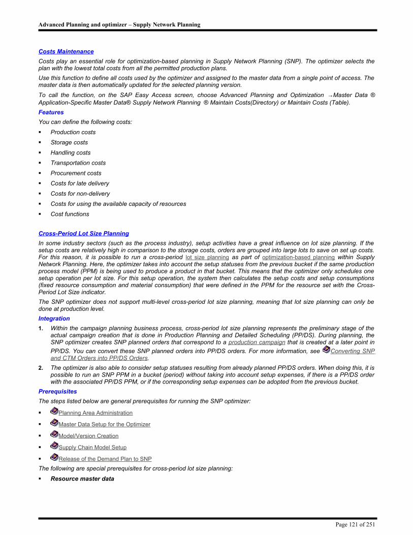
Advanced Planning and optimizer – Supply Network Planning

Costs Maintenance

Costs play an essential role for optimization-based planning in Supply Network Planning (SNP). The optimizer selects the plan with the lowest total costs from all the permitted production plans.

Use this function to define all costs used by the optimizer and assigned to the master data from a single point of access. The master data is then automatically updated for the selected planning version.

To call the function, on the SAP Easy Access screen, choose Advanced Planning and Optimization →Master Data ® Application-Specific Master Data® Supply Network Planning ® Maintain Costs(Directory) or Maintain Costs (Table).

Features

You can define the following costs:

Production costs

Storage costs

Handling costs

Transportation costs

Procurement costs

Costs for late delivery

Costs for non-delivery

Costs for using the available capacity of resources

Cost functions

Cross-Period Lot Size Planning

In some industry sectors (such as the process industry), setup activities have a great influence on lot size planning. If the setup costs are relatively high in comparison to the storage costs, orders are grouped into large lots to save on set up costs. For this reason, it is possible to run a cross-period lot size planning as part of optimization-based planning within Supply Network Planning. Here, the optimizer takes into account the setup statuses from the previous bucket if the same production process model (PPM) is being used to produce a product in that bucket. This means that the optimizer only schedules one setup operation per lot size. For this setup operation, the system then calculates the setup costs and setup consumptions (fixed resource consumption and material consumption) that were defined in the PPM for the resource set with the Cross-Period Lot Size indicator.

The SNP optimizer does not support multi-level cross-period lot size planning, meaning that lot size planning can only be done at production level.

Integration

1. Within the campaign planning business process, cross-period lot size planning represents the preliminary stage of the actual campaign creation that is done in Production Planning and Detailed Scheduling (PP/DS). During planning, the SNP optimizer creates SNP planned orders that correspond to a production campaign that is created at a later point in

PP/DS. You can convert these SNP planned orders into PP/DS orders. For more information, see Converting SNP and CTM Orders into PP/DS Orders.

2. The optimizer is also able to consider setup statuses resulting from already planned PP/DS orders. When doing this, it is possible to run an SNP PPM in a bucket (period) without taking into account setup expenses, if there is a PP/DS order with the associated PP/DS PPM, or if the corresponding setup expenses can be adopted from the previous bucket.

Prerequisites

The steps listed below are general prerequisites for running the SNP optimizer:

Planning Area Administration

Master Data Setup for the Optimizer

Model/Version Creation

Supply Chain Model Setup

Release of the Demand Plan to SNP

The following are special prerequisites for cross-period lot size planning:

Resource master data

Page 121 of 251

Advanced Planning and optimizer – Supply Network Planning

The optimizer only takes into account the setup statuses from previous buckets for the resource for which the cross-period lot size indicator has been set.

Production process model (PPM)

1. The PPM is permitted to use a maximum of one resource only for which the cross-period lot sizeindicator has been set.

2. The PPM is not permitted to use any other resources that have been specified with a fixed resource consumption.

3. The PPM duration must be less than or equal to the smallest bucket from the planning buckets profile used.

4. The minimum PPM lot sizes and the discrete (integer value) lot sizes refer to the cross-period lot quantity.

5. The optimizer plans a maximum of one setup operation per bucket.

Profiles

In Supply Network Planning, you have also maintained the relevant profiles for SNP optimization, in particular the SNP optimizer profile (from the Implementation Guide (IMG), choose SAP Advanced Planner and optimizer (SAP APO) ® Supply Chain Planning ® Supply Network Planning ® Profiles ® Define SNP Optimizer Profiles). For more information, see Optimization Profiles and the corresponding Implementation Guide (IMG) documentation.

In particular, you have made the following settings for cross-period lot size planning in the SNP optimizer profile:

You have chosen Discrete Optimization as your optimization method.

You have entered the horizon over which you want the optimizer to take into account the setup statuses from this previous bucket in the Cross-Period Lot Size field from the Discrete Constraints tab page. The optimizer can only do this if the PPM from the previous bucket is used to produce a product.

If you want the optimizer to take account of setup statuses resulting from already planned PP/DS orders, you must have activated the indicator Cross-Period Lot Size Planning on the Integration tab page. A prerequisite for this is that the corresponding PP/DS PPM must be assigned to the SNP PPM.

Activities

You run the optimizer from the interactive planning desktop or in the background. For more information, see Running the Optimizer from the Interactive Planning Desktop and Running the Optimizer in the Background. For general information on the SNP optimizer, see Optimization-Based Planning.

The optimizer determines the most cost-effective solution to fulfil the demands. For example, to decide about lot sizes, the optimizer uses storage costs and setup costs. Having larger lot sizes and only one setup operation per lot size saves on setup costs but results in higher storage costs. With smaller lot sizes, multiple setups mean that more capacity is required and this results in higher setup costs.

You display the individual stages and final results of the optimization run in interactive planning on the Optimization tab page within the optimizer window. You also receive a list of the costs determined by the optimizer.

Application Logs for Optimizers

When you execute an optimization-based planning function in Supply Network Planning (SNP) in the background (mass processing), the system automatically generates an application log. Amongst other things, this log contains planning results,

Page 122 of 251

Advanced Planning and optimizer – Supply Network Planning

such as planned orders and stock transfers created, as well as error, warning, and information messages. The input data for the optimization run and the costs of the solution determined by the optimizer are also displayed, for example.

The central Optimizer Log Data function is available for accessing optimization run logs. From the SAP Easy Access screen, choose Advanced Planning and Optimization ® Supply Network Planning ® Reporting ®Optimizer Log Data. You can use this function to access the following SNP planning functions:

SNP Optimizer

Deployment Optimizer

Capacity Leveling (optimization-based method)

Sourcing of Forecast

Features

The Optimizer Log Data function provides an overview of the generated logs. Amongst other things, the list of logs contains the following data:

Log status

A traffic light or flag indicates whether the optimization run is still in progress, has already ended, or was terminated with a message (see F1 help).

Log creator

Optimizer profile used

Start and finish time of the run

Runtimes of the individual optimization steps

An optimization run has three steps (data reading, model consistency check, and solution calculation, as well as order creation).

Total costs of solution

Log expiration date

You specify the log expiration date globally for all optimization logs in Customizing for Advanced Planning and Optimization (APO) under Basis Settings → Optimization ® Basic Functions ® Maintain Global Settings. However,

you can also change this date for one specific optimization run by choosing Change Expiration Date. The log is automatically deleted after the expiration date if you execute the /SAPAPO/OM_REORG_DAILY report.

You can also delete the log from the list, set filters and sort entries.

If you double click a log or choose Display Log, you receive the following data and sub-logs for the log.

Input Parameter

Contains the settings that you made on the initial screen for the planning function.

Location Products

Contains the location products selected for the optimization run.

Deletion Time Period

Specifies a time period in which the system deletes existing planned orders and stock transfers before actual optimization.

Input Log

Contains the input data considered by the system during the optimization run (that is, master data and transaction data). The data is divided into a number of tables (such as ET_LOCMAT). You can display the content of these tables on the right-hand side of the screen. For more information, see Optimization Input Log.

Results Log

Contains all results of the optimization run, such as planned orders, stock transfers, resource consumption, costs, and penalty costs. The data is divided into a number of tables (such as ET_PROMO). You can display the content of these tables on the right-hand side of the screen.

Result Indicators

Contains indicators that display the quality of the optimization solution, such as service level and shortfall of safety stock. For more information, see Result Indicators.

Explanations

Contains the results of an explanation tool run (see below).

Extended Results Log

Page 123 of 251

Advanced Planning and optimizer – Supply Network Planning

In this log, you can display the results of the optimization run in the interactive SNP planning form.

Message Log

Contains error messages, warning messages, and information messages generated by the system during the optimization run. They are ordered according to meaning, that is, whether they refer to the optimization run settings or to the three main steps of the run.

Trace File

All individual optimization run steps are logged in this text file. It is saved on the optimization server, but you can also download it to your own computer.

Costs

Contains detailed information about the costs of the solution determined by the optimizer. For more information, see Resulting Costs of Optimization.

Solution Quality

Contains the costs of the best solution determined by the optimizer up to the time displayed. If you used a decomposition method, you can also relate the costs the partial problem solved up to this time.

You can use the log to determine whether you can reduce the optimizer runtime without effecting solution quality.

Note that the input log and the results log, as well as the deletion time period, are only displayed if you have set the Write All Log Data indicator in the optimizer profile being used. Even if an error occurred in the first step of the optimization run (data reading), the log may not be available.

You can also download the input log and the results log to your own computer. To do this, choose Download

Input Log or Download Results Log. The logs are then saved in RELATIOM text format.

If you select a log and choose Explain, you go to the Explanations of SNP Optimization Resultsscreen. From this screen you can execute the explanation tool which explains two important exceptional situations of an optimization run: non-deliveries and shortfall of safety stock.

Optimization Input Log

Log generated during an optimization run in Supply Network Planning (SNP). It contains all input data considered by the system during the optimization run (that is, master data and transaction data). The data is utilized in numerous tables (such as ET_LOCMAT).

Use

The input log is part of the application log that you can access by selecting Advanced Planning and Optimization ® Supply Network Planning ® Reporting ® Optimizer Log Data from the SAP Easy Access screen. For more information, see Application Logs for Optimizer.

You can download the log and give it to SAP support as a text file for analysis.

Structure

The individual sections of the log are detailed below.

Legend

Flag: X = Active, ' ' = Inactive

Prof: SNP optimizer profile

Units: BTime = Base unit of time (days)

BCurr = Base currency

BProd = Base unit of measure of the product

HanUn = Handling unit

StoUn = Storage unit

BRes = Base unit of measure of the resource

ES_CTRL

These entries describe the general properties of the model. The entries are determined from the SNP optimizer profile or directly from the model. Discrete (integer value) transportation lots are displayed in the history of the optimization runs (the ‘trace file’); choose Tools → APO Administration → Optimization →Log Display.

NBUCK Number of buckets

NPROD Number of products

Page 124 of 251

Advanced Planning and optimizer – Supply Network Planning

NLOCS Number of locations

NSUBL Number of sublocations

NPROM Number of production process models

NRESO Number of resources

NREFA Number of resource families

NARCS Number of arcs

NFLEE Number of fleets

NDEMC Actual number of demand classes

NDEMA Number of demand vectors

DISRF Prof: End bucket for increasing production resource discretely

DISRZ Prof: End bucket for using fixed production resource consumption

DISTR Prof: End bucket for using discrete fleet on transportation lanes

DISPR Prof: End bucket for using integral PPM

KAMPA Prof: End bucket for campaign + D416 planning

TRLOS Prof: End bucket for using minimum transportation lot size

PRLOS Prof: End bucket for using minimum production lot size

COSTR Prof: End bucket for using transportation cost function

COSPD Prof: End bucket for using production cost function

COSPC Prof: End bucket for using procurement cost function

ET_INEXKEY

These entries are the external keys for internal object keys. In particular, there is a list of calendar data for the day numbers, and a list of product and location numbers for the GUIDs.

INKEY GUID (unique internal key)

EXKEY Corresponding external key

ET_BUCKDF

These entries show the bucket definition (time intervals) upon which all optimizer planning is based. The source of this information is either the selected planning buckets profile or the planning start and end date.

BUCKE* Bucket no.

VALTO End date of the bucket (day no., 1st day is 1/1/1970) BTime

VALFR Begin date of the bucket (day no., 1st day is 1/1/1970) BTime

ET_MATERIAL

The validity period of all products selected for optimization is stored here. At present, this always encompasses the entire planning horizon.

MATID* Product GUID

BCKTO Valid to bucket no.

BCKFR Valid from bucket no.

ET_LOC

Information about the existence or non-existence of a defined handling capacity (handling resource) is stored here for locations.

LOCID* Location GUID

RESIN Handling-in resource GUID or dummy resource, if no handling-in resource is maintained

MAXIN Prof: Flag: Handling-in resource active (not activated, if dummy resource is used)

RESOU Handling-out resource GUID or dummy resource, if no handling-out resource is maintained

MAXOU Prof: Flag: Handling-out resource active (not activated, if dummy resource is used)

Page 125 of 251

Advanced Planning and optimizer – Supply Network Planning

ET_SUBLOC

A storage resource is defined here with information about whether it can be extended. SUBID is currently the resource ID. The source of this information is the location master and, if in existence, storage resource maintenance. Extension is allowed if the resource has two capacity variants.

SUBID* Storage resource GUID or dummy resource, if no storage resource is maintained

MAXFL Prof: Flag: Storage resource active (not activated, if dummy resource is used)

ET_LOCMAT

The properties of location-dependent products are shown here. Resource consumption is listed, in particular. The source for this is the location product master.

LOCID* Location GUID

MATID* Product GUID

SUBID Storage GUID

HCOST Storage cost BCurr/BProd

BUCFL Prof: Flag: Storage cost: Multiply by bucket length

SSPEN Penalty for not covering safety stock BCurr/BProd

MAXST Maximum stock level of the product

MAXFL Flag: Maximum stock level active

STOCK Initial stock BProd

CONIN Consumption of input handling capacity HanUn/BProd

COSIN Handling-in cost BCurr/BProd

CONOU Consumption of output handling capacity HanUn/BProd

COSOU Handling-out cost BCurr/BProd

RECTI Goods receipt processing time in days BTime

ISSTI Goods issue processing time in days BTime

CACON Storage capacity consumption StoUn/BProd

WASFL Flag: Shelf life penalty is active

WASTE Shelf life: Penalty for wasted quantity BCurr/BProd

STODU Shelf life: Storage duration BTime

FCOST Linear procurement cost BCurr/BProd

FPERF Procurement permitted and/or product subject to incremental optimization

SSMTH Safety stock method

ET_RESOURCE

Production resources that are used in the production process models are listed here (see the ET_PRORES section below). UNIVO is currently always equal to 1.

RESID* Resource GUID

RFAID Resource family GUID (currently the same as resource)

UNIVO Unitary volume BRes

KAMPA Flag: Resource is a campaign resource

ET_RESFAM

Production resources are allowed to be extended here if a second capacity variant has been defined in the resource master. The resource family is currently always the same as the production resources (one-to-one).

RFAID* Resource family ID

MAXFL Flag: Resource has a capacity constraint

DISCR Prof: Flag: Discrete increase of resource family

ET_FLEET

Fleet refers to the transportation resource that has been specified for a transportation lane. A possible extension and the costs related to it are determined from the resource’s second capacity variant.

FLEID* Fleet GUID

Page 126 of 251

Advanced Planning and optimizer – Supply Network Planning

MAXFL Flag: Consider maximum fleet capacity

TUNIA Capacity 1 of one truck TraUn1

TUNIB Capacity 2 of one truck (not used) TraUn2

TUNIC Capacity 3 of one truck (not used) TraUn3

ET_ARC

All the transportation lanes that have been defined for the model in the Supply Chain Engineer are listed here. ARC refers to a transportation lane/means of transport combination.

ARCID* Arc GUID

FLEID Fleet GUID

LOCFR Location from GUID

LOCTO Location to GUID

TTYPE ID for means of transport

DURAT Duration of shipment (base time unit) BTime

RNDTR Bucket offset (rounding limit for transportation times)

TCTYP Variable transportation cost for the fleet BCurr/TraUn1

DISCR Flag: Using discrete transportation fleets

RLDUR Resource load duration BTime

ET_ARCMAT

Product-dependent properties for the transportation lane are shown here. Data is taken from the Supply Chain Engineer. Standard entries are generated if the product has not been assigned to the transportation lane and the All Products indicator has been set at the transportation lane. The lot size information is taken from the lot size profile (transportation lanes) defined at the transportation lane.

ARCID* Arc GUID

MATID* Product GUID

VALTO Valid to date (base unit of time) BTime

VALFR Valid from date (base unit of time) BTime

MINLO Minimum number of lots TRVOL

MAXLO Maximum number of lots TRVOL

MAXFL Flag: MAXLO active

TRVOL Lot size in product units BProd

TCONA Capacity consumption for 24 hours TraUn1/BProd

TCONB Capacity consumption for the transportation time that is less than 24 hours TraUn1/BProd

TCONC Capacity consumption (not used)

TCOST Variable transportation cost for "arc product" BCurr/BProd

SUBCO Flag: ‘X’ Product will be subcontracted

ET_LOCC

The handling resource’s available capacity is listed here. Figures are determined from the resource’s first capacity variant. Gaps in the intervals are defined by the resource calendar or shipping calendar of the location.

RESID* Handling resource GUID

VALTO* Valid to date (base unit of time) BTime

VALFR Valid from date (base unit of time) BTime

MAXHA Handling capacity HanUn/BTime

COUND Minimum resource consumption

UNPEN Penalty per unitary volume dropping minimum capacity BCurr/Univo

Page 127 of 251

Advanced Planning and optimizer – Supply Network Planning

ET_LOCUC

A possible extension of the handling resource’s available capacity is listed here. Figures are determined from the resource’s second capacity variant by subtracting the first capacity variant values. Gaps in the intervals are defined by the resource calendar or shipping calendar of the location.

RESID* Handling resource GUID

VALTO* Valid to date (base unit of time) BTime

VALFR Valid from date (base unit of time) BTime

INCHA Upper bound for increasing handling capacity HanUn/BTime

INPEN Penalty per unitary volume for increasing capacity BCurr/Univo

ET_SUBLOCC

The storage resource’s available capacity is listed here. Figures are determined from the resource’s first capacity variant. The interval gaps are defined by the resource calendar.

SUBID* Sublocation GUID

VALTO* Valid to date (base unit of time) BTime

VALFR Valid from date (base unit of time) BTime

MAXSL Capacity volume of storage (sublocation) StoUn

COUND Minimum resource consumption

UNPEN Penalty per unitary volume dropping minimum capacity BCurr/Univo

ET_SUBLOCUC

A possible extension of the storage resource’s available capacity at a location is listed here. Figures are determined from the resource’s second capacity variant by subtracting the first capacity variant values. The interval gaps are defined by the resource calendar.

SUBID* Sublocation (storage) GUID

VALTO* Valid to date (base unit of time) BTime

VALFR Valid from date (base unit of time) BTime

INCSL Upper bound for increasing storage capacity StoUn

INPEN Penalty per unitary volume for increasing capacity BCurr/Univo

ET_RESC

The production resource’s available capacity is listed here. Figures are determined from the resource’s first capacity variant. The interval gaps are defined by the resource calendar.

RESID* Resource GUID

VALTO* Valid to date (base unit of time) BTime

VALFR Valid from date (base unit of time) BTime

MAXRE Production resource capacity BRes/BTime

COUND Minimum resource consumption

UNPEN Penalty per unitary volume dropping minimum capacity BCurr/Univo

CCOST Cost per unitary volume for capacity BCurr/Univo

ET_RESFAMC

A possible extension of the production resource’s available capacity is listed here. Figures are determined from the resource’s second capacity variant by subtracting the first capacity variant values. The interval gaps are defined by the resource calendar.

RFAID* Resource family GUID

VALTO* Valid to date (base unit of time) BTime

VALFR Valid from date (base unit of time) BTime

INCRF Upper bound for increasing production resource Univo/BTime

INPEN Penalty per unitary volume for increasing capacity BCurr/Univo

Page 128 of 251

Advanced Planning and optimizer – Supply Network Planning

ET_FLEETC

The transportation resource’s available capacity is listed here. Figures are determined from the resource’s first capacity variant. The interval gaps are defined by the resource calendar.

FLEID* Fleet GUID

VALTO* Valid to date (base unit of time) BTime

VALFR Valid from date (base unit of time) BTime

MAXFL Capacity measured in trucks Truck/BTime

COUND Minimum resource consumption

UNPEN Penalty per unitary volume dropping minimum capacity BCurr/Truck

ET_FLEETUC

A possible extension of the transportation resource’s available capacity is listed here. Figures are determined from the resource’s second capacity variant by subtracting the first capacity variant values. The interval gaps are defined by the resource calendar.

FLEID* Fleet GUID

VALTO* Valid to date (base unit of time) BTime

VALFR Valid from date (base unit of time) BTime

INCFL Upper bound for increasing fleet capacity Truck/BTime

INPEN Penalty per unitary volume for increasing capacity BCurr/Truck

ET_PROMO

The properties of the production process model (plan or PPM) are stored here. However, the PPM needs to have been assigned to the model in the Supply Chain Engineer. This information is defined in master data maintenance for the PPM. Time-dependent PPMs are converted into multiple entries for the optimizer, and the validity period of each one is set accordingly. The master resource is the PPM calendar resource.

PROID* Production process model GUID

LOCID Location GUID

MATID Product GUID

LOTSZ Fixed lot size of the location product BProd

BCKTO Valid to date in buckets

BCKFR Valid from date in buckets

PMINQ Minimum production lot size ProMod

PMAXQ Maximum production lot size ProMod

MAXFL Flag: PMAXQ active

DURAT Duration: 0 = one day, 1 = two days BTime

DISCR Flag for using discrete production

PCOST Variable cost of PPM BCurr/ProMod

RNDPR Bucket offset

RESID Resource GUID for calendar

ET_PRORES

Consumption of production resources for the PPM is listed here, as defined in the production process model master data in Mode →Capacity Consumption.

PROID* Production process model GUID

RESID* Resource GUID

OFSTO* Consumption time offset BTime

BCKTO* Valid to date of bucket interval

VCONS Variable consumption of the resource BRes

FCONS Fixed consumption of the resource BRes

Page 129 of 251

Advanced Planning and optimizer – Supply Network Planning

ET_PROMAT

The product flow for the PPM, as defined in the Products section of production process model master data, is listed here. It represents the bill of materials (BOM) structure, where finished products have a plus sign and input products a minus sign.

PROID* Production process model GUID

MATID* Product GUID

OFSTO* Input/output time offset BTime

LOCID* Location GUID

BCKTO* Valid to date of bucket interval

OUTIN Output(+) or input(-) quantity BProd

FCONS Fixed input(-) quantity BProd

ET_RESINI

Contains the initial setup statuses of the resources for cross-period lot size planning (set up or not set up).

RESID* Resource GUID

PROID* Production process model GUID

EDATE* End date BTime

BDATE* Start date BTime

QUANT Output quantity for master product BProd

APPLI Application: P->PP/DS S->SNP

SETUP Flag: Order with setup

ET_LOCPROD

The required safety stock (target stock levels), fixed demands (FPROD with minus sign), and receipts for the products are defined in this table. The latter entries result from planned orders and stock transfers that had been fixed before the optimizer was run. This fixing is done both manually and when orders are transferred to the PP/DS application. Receipts and issues are also fixed when the optimizer has been run incrementally (for a subset of products from the model).

LOCID* Location GUID

MATID* Product GUID

BUCKE* Date bucket of safety stock and FPROD

SAFTY Safety stock (not a demand!) BProd

MAXST Maximum stock level of the product BProd

SAPEN Penalty for not covering safety stock BCurr/BProd

STPEN Penalty for violating the maximum stock level BCurr/BProd

FPROD Confirmed production, includes intransit quantities BProd

SVTTY Safety days’ supply

ET_DEMCLTIM

The maximum delay that is to be allowed for finished products is defined here. The values are taken from the product master (the SNP 1 tab page). There are currently only three categories: 1 for customer demands, 2 for corrected demand forecasts, and 3 for demand forecasts. Costs for delivering the finished products late, or for not delivering them at all are also defined. The values are taken from the product master (the SNP 1 tab page). The values are not defined as time-dependent in SAP APO, meaning that BCKTO is the same as the planning end date.

DEMCL* Demand class (highest priority = 1)

LOCID* Location GUID

MATID* Product GUID

BCKTO* Valid to bucket

LAPEN Penalty for lateness BCurr/(BTime*BProd)

MAXLA Maximum lateness BTime

NDPEN Penalty for not delivering BCurr/BProd

ET_DEMAND

This table contains all the customer demands and forecast demands that have been read for the model from liveCache.

Page 130 of 251

Advanced Planning and optimizer – Supply Network Planning

LOCID* Location GUID

MATID* Product GUID

DEMCL* Demand class (highest priority = 1)

BUCKE* Demand date given in bucket

DEMAN Quantity of demand BProd

ET_PROCBND

Target procurement corridor.

LOCID* Location GUID

MATID* Product GUID

BUCKE* Bucket

LOWBN Lower bound BProd

UPPBN Upper bound BProd

INITV Initial value (result of previous run) BProd

BNDFL Flag: Upper bounds are active

ET_PRODBND

Target production corridor.

PROID* Production process model GUID

BUCKE* Bucket

LOWBN Lower bound ProMod

UPPBN Upper bound ProMod

INITV Initial value (result of previous run) ProMod

BNDFL Flag: Upper bounds are active

ET_TRANBND

Target stock transfer corridor.

ARCID* Arc GUID

MATID* Product GUID

BUCKE* Bucket

LOWBN Lower bound BProd

UPPBN Upper bound BProd

INITV Initial value (result of previous run) BProd

BNDFL Flag: Upper bounds are active

ET_STCKBND

Target stock level corridor.

LOCID* Location GUID

MATID* Product GUID

BUCKE* Bucket

LOWBN Lower bound BProd

UPPBN Upper bound BProd

INITV Initial value (result of previous run) BProd

BNDFL Flag: Upper bounds are active

ET_DELIBND

Target demand fulfillment corridor.

LOCID* Location GUID

MATID* Product GUID

DEMCL* Demand class (highest priority = 1)

DELAY* Lateness measured in buckets

Page 131 of 251

Advanced Planning and optimizer – Supply Network Planning

BUCKE* Bucket

LOWBN Lower bound BProd

UPPBN Upper bound BProd

INITV Initial value (result of previous run) BProd

BNDFL Flag: Upper bounds are active

ET_TRANCOS

Stock transfer cost functions are defined here. These functions are analyzed on the basis of this formula: Cost = FIXCO + VARCO* (X – ORIGN). The cost function is assigned to the product-dependent transportation lane in the Supply Chain Engineer.

ARCID* Arc GUID

ORIGN* Smallest value TraUn1

FIXCO Fixed cost BCurr

VARCO Variable cost BCurr/TraUn1

ET_PRODCOS

Production cost functions are defined here. These functions are analyzed on the basis of this formula: Cost = FIXCO + VARCO* (X – ORIGN). The cost function is assigned to the plan in master data maintenance for the production process model.

PROID* Production process model GUID

ORIGN* Smallest value ProMod

FIXCO Fixed cost BCurr

VARCO Variable cost BCurr/ProMod

ET_PROCCOS

Procurement cost functions are defined here. These functions are analyzed on the basis of this formula: Cost = FIXCO + VARCO* (X – ORIGN). This cost function is assigned to the product in the location product master.

LOCID* Location GUID

MATID* Product GUID

ORIGN* Smallest value BProd

FIXCO Fixed cost BCurr

VARCO Variable cost BCurr/BProd

Resulting Costs of Optimization

Log generated during an optimization run in Supply Network Planning (SNP). It contains detailed information about the costs of the solution determined by the optimizer.

Use

The log is part of the application log that you can access by selecting Advanced Planning and Optimization ® Supply Network Planning ® Reporting ® Optimizer Log Data from the SAP Easy Access screen. For more information, see Application Logs for Optimizers.

Structure

The individual fields of the log are detailed below.

Field Information displayed

User The planner's name.

Current date The date the Optimization run was executed.

Time The time when the Optimization run was executed..

version The planning version used for the optimization run.

Optimizer profile The optimizer profile used for optimization run.

Cost profile The cost profile used for optimization run.

Bound profile The SNP optimization bound profile used for optimization run.

Page 132 of 251

Advanced Planning and optimizer – Supply Network Planning

Field Information displayed

Total costs The total costs associated with the solution proposed by the system. The cost categories are displayed in total values for all objects throughout the supply chain. The total costs are made up of all the cost categories displayed in this log.

Production costs The total production costs for this plan based on the pieces produced using the production process models PPMs with the associated cost data, displayed in total values for all objects throughout the supply chain.

Procurement costs The total procurement costs for this plan.

Storage costs The total storage costs for this plan based on the capacity consumption of products stored at the storage resource, displayed in total values for all objects throughout the supply chain.

Storage expansion The total costs incurred as a result of a requirement to expand storage capacity for this plan displayed in total values for all objects throughout the supply chain.

Penalty costs for safety stock deficit

The total penalty costs incurred because the safety stock level falls below the specified requirement for safety stock for this plan displayed in total values for all objects throughout the supply chain.

Transportation costs The total transportation costs for this plan displayed in total values for all objects throughout the supply chain.

Handling capacity expansion

The total costs incurred as a result of a requirement to expand the handling capacity of one or more resources for this plan displayed in total values for all objects throughout the supply chain.

Transportation capacity expansion

The total costs incurred as a result of a requirement to expand the transportation resource capacity for this plan displayed in total values for all objects throughout the supply chain.

Production resource expansion

The total costs incurred as a result of a requirement to expand the production resource capacity for this plan displayed in total values for all objects throughout the supply chain.

Delay penalty The total penalty costs incurred as a result of all deliveries that are late displayed in total values for all objects throughout the supply chain.

Shortfall penalty The total penalty costs incurred as a result of all deliveries of all products that are less than the quantity ordered displayed in total values for all objects throughout the supply chain.

Penalty costs for exceeding maximum stock on hand

The total penalty costs incurred for exceeding maximum stock on hand.

Penalty costs for falling short of minimum resource utilization

The total penalty costs incurred for falling short of the minimum resource utilization defined in the resource master data.

Result Indicators

Indicators that show the quality of an optimization solution.

Use

If you have successfully executed an optimization run and have created a log for this run, the log contains a series of result indicators. They show the quality of the optimization solution with reference to the following factors:

Demand Fulfillment

Stock Level

Resource Utilization

From the SAP Easy Access screen, you choose Advanced Planning and Optimization →Supply Network Planning → Reporting →Optimizer Log Data. You then select an optimization run with a double-click. The tree structure of the logs contains the entry Result Indicatorswith the two aggregation levels Model-Dependent Indicators and Location Product-Dependent Indicators.

Structure

The system calculates the following indicators for the quality of an optimization solution:

Demand Fulfillment

Service level (in percent)

Delayed demand fulfillment (in percent)

Page 133 of 251

Advanced Planning and optimizer – Supply Network Planning

Average delay (in days)

The system also calculates these indicators separately for the following priority classes:

Customer requirement

Demand forecast

Corrected demand forecast

“Pseudo-hard” demand (if you have made the setting in the optimizer profile that the system considers the dependent demand and/or distribution demand of fixed orders as a pseudo-hard constraint. That means that the system may allow shortages for which it calculates penalty costs).

Stock Level

Fulfillment of safety stock demand in percent

Average stock level

Utilization

The system calculates the resource consumption for the following resource types.

Production resources

Storage resources

Transportation resources

Handling resources

You can also display the resource utilization for each period in the capacity view of interactive SNP planning. The capacity view always shows the current resource utilization based on the data saved in liveCache. However, the data calculated by the explanation tool is available for as long as the output log of the optimization run is available.

The system calculates the result indicators at the level of the model and each location product or resource, and displays this data directly in the optimization run log or under the Result Indicators entry. The indicators for the utilization of the individual resources are displayed in the result log.

To aggregate the data of each location product at different levels (such as location level or product level), you can transfer the data to the SAP NetWeaver Usage Type Business Intelligence (BI) using the DataSource 0APO_SNP_INDICATOR. For more information, see the documentation for component SAP NetWeaver under BI Content → Supply Chain Management → Planning. You can also simulate a simple aggregation with the SAP List Viewer (ALV).

The following table shows the aggregation levels at which the result indicators are displayed in the optimization log:

Service Level

Delay in Percent

Average Delay

Service Level per Demand Class

Delay in Percent per Demand Class

Average Delay per Demand Class

Average Stock Level

Safety Stock Shortfall

Utilization per Resource

Model x x x x x x x x

Location Product

x x x x x x x x

Resource

x

Explanation of the Optimization Results

Optimization-based planning in Supply Network Planning (SNP) pursues a global solution approach by considering all restrictions and costs simultaneously and across the entire model. It therefore frequently finds a better solution than is possible with other planning methods. However, the results of the optimization run are not always easy to understand.

You can use the explanation tool to have the system explain two significant exceptional situations of an optimization run:

Non-delivery

Shortfall of safety stock

This function shows you the possible causes for the exceptional situations in the optimization run log. You can use the causes shown to check whether you can solve the problem by increasing capacities or extending horizons, for example. The system also suggests additional orders that you could use to remedy the missing quantities.

Among other things, you can specify the location products for which you want the explanation, and how detailed it should be.

Page 134 of 251

Advanced Planning and optimizer – Supply Network Planning

Prerequisites

You have executed an optimization run and created a log for this run (that is, you have set the Write All Log Data indicator in the SNP or deployment optimizer profile). The explanation tool refers to the result of the optimization run as you see it in the log.

Between the optimization run and explanation run, you have not changed the SNP or deployment optimizer profile you used for the optimization run. You have also not changed the optimization-relevant settings in planning version management.

In the case of a deployment optimization run, you have chosen an optimal cost allocation. The explanation tool does not support fair share or push distribution.

Features

Non-deliveries and lack of safety stock can have the following five causes:

Capacity Constraints

Time-Based Constraints and Maximum Lot Sizes

Product Availability

Lead Time

Costs

The explanation tool displays these causes, but does not explain why the optimizer fulfills the demand of one product but not of another when there is a lack of capacity.

Capacity Constraints

In the SNP or deployment optimizer profile, you have defined that the optimizer is to consider certain capacity constraints. The optimizer considers the resource capacity defined in the resource master data.

A possible cause for non-deliveries is that the system cannot fulfill the demand with the available resource capacity.

The system shows you the following data of the capacity problem:

Resource with the capacity problem.

Number of the period (bucket) where the capacity problem occurs.

Missing capacity of the resource.

If your planning buckets profile also includes daily periods, the system cannot determine any capacity problems caused by calendar problems within the time frame covered by daily periods. For example, the system cannot suggest working on a holiday could make up capacity.

Time-Based Constraints and Maximum Lot Sizes

In interactive SNP planning, you have defined time-based constraints (upper limits) for the capacity of specific sources of supply (such as for production or transportation). For more information, see Definition of Time-Based Constraints in Interactive Planning. In the SNP or deployment optimizer profile, you have also or alternatively defined that the optimizer is to consider maximum lot sizes.

The system displays the following data:

Name of the source of supply for which you have set the upper limit or maximum lot size.

Name of the product for which you have set the upper limit or maximum lot size.

Procurement type of the location product (in-house production, external procurement, and so on).

Number of the period where the capacity problem occurs.

Quantity by which you must raise the upper limit to solve the problem. In the case of the production upper limit, the system does not show the quantity but rather the number of executions of the production model (PPM) or production data structure (PDS). An execution of the PPM or PDS corresponds to the output quantity you specified in the PPM/PDS.

Product Availability

A possible cause for non-delivery can be that products are not available because a source of supply does not exist (for example, because the bill of material has not been completely defined).

The system shows you the following data of the product availability:

Name of the product and location

Number of the period in which the product quantity is missing

Missing quantity of the product

Page 135 of 251

Advanced Planning and optimizer – Supply Network Planning

The system does not check the validity of PPMs/PDSs or transportation lanes. It also does not check the validity of time-dependent parameters of PPMs/PDS (such as material consumption).

If you have defined a PPM/PDS that is not valid until the middle of the planning horizon, for example, the system does not determine any availability problems in the first half of the planning horizon.

Lead Time

Due to a long duration of shipment and production, the lead time it takes for a product to be available in a specific period can stretch over several periods. The system therefore frequently cannot fulfill demands because the lead time stretches into the production or stock transfer horizon, or the planned delivery time. The lead time can even stretch back into the past (before the planning period).

The system shows you the following data of the lead-time:

Name of the product and location

Name of the source of supply

Procurement type of the location product

If the lead-time stretches into the past, the procurement type is S (initial stock level).

Missing quantity of the product

Start and finish time of the order

Number of days by which the corresponding horizon (production or stock transfer horizon) or the planned delivery time has been violated.

Costs

The fulfillment of the demand and the safety stock requirement is called a soft constraint for the SNP or deployment optimizer. That means there are penalty costs for not fulfilling the demand. If you have set the penalty costs for non-delivery and safety stock shortfall too low in the location product master data, the optimizer may decide not to fulfill the demand. This may be the case if the total costs are lower when demand is not fulfilled.

The system displays this possible cause in a message.

If you have not defined penalty costs for safety stock shortfall, the optimizer cannot determine the cause. If you run a model consistency check, you will, however, see a corresponding message.

Order Suggestions

The system suggests additional orders that you could use to remedy the missing quantities.

If you use the suggested orders or try to solve the exceptional situations another way depending on the displayed causes, a new optimization run can however still lead to similar or different problems due to the dependencies.

For example, if you increase the capacity of a resource to remedy the missing quantities of a specific product, the system can use the additional capacity to cover the missing quantities of another product with higher priority.

Further Information

The explanation tool only generates one possible explanation for each exceptional situation. However, there may be other explanations as well. For example, if the system finds a capacity bottle-neck for a resource and suggests increasing the capacity of this resource, another solution might be to increase the capacity of an alternative resource.

If the results of the explanation tool are incorrect, this might be because the optimization solution on which they are based was not optimal (for example, due to runtime restrictions).

Activities

To execute the explanation tool, from the SAP Easy Access screen, choose Advanced Planning and Optimization ® Supply Network Planning ® Reporting ® Optimizer Log Data. Then select an optimization run and choose Explain. The Explanations of the SNP Optimization Results screen appears. Here you make settings such as the target and level of detail of the explanation, and choose Execute. For more information, see Configuration of the Explanation Tool.

After you have executed the explanation run, you see the Optimization Run X screen that displays the logs for the selected optimization run. The tree structure contains the entry Explanations with the subentries Configuration and Explanation Results. If you double-click on these entries, you see your entry data and/or the results of the explanation run on tab pages on the right side of the screen. If the upper table on the right side of the screen contains several entries, you can double-click on an entry in the lower table to see its detailed data.

You can also execute the explanation tool from the Optimization Run X screen by choosing Explain.

If you want to execute the explanation tool in the background, choose Advanced Planning and Optimization ® Supply Network Planning ® Reporting ® Explanation of Optimization Results.

Page 136 of 251

Advanced Planning and optimizer – Supply Network Planning

Configuration of the Explanation Tool

You can configure the explanation tool for an optimization log in Supply Network Planning (SNP) according to your requirements. This means you can choose which exceptional situations you want explained and how detailed you want the explanation to be. This affects, for example, the complexity of the calculation and thus the runtime as well.

Process:

1. Selection of the Optimization Run

You can select a specific optimization run directly or you can specify which run of a specific user is to be explained (going backward: the fourth to last run is run no. 4, for example).

2. Target of the Explanation

You can specify whether you want an explanation for the causes for non-delivery only, or for the causes for safety stock shortfall only, or both. In addition, you can specify the priority classes of the demand for which you want the system to determine these causes (demand forecast, customer demand, and so on).

You also have to show the system how your model is structured. By doing so, you are giving the system information about the sequence in which it is to check the possible causes for an exceptional situation. Depending on whether your model is based on control costs or actual costs or whether it is in the structure phase, other causes for the exceptional situation could be possible. Since the causes are dependent on one another, the check sequence of these causes is crucial for the analysis.

The following table shows the sequence of the analysis depending on the model:

Model based on control costs

(Such as high non-delivery costs with the goal of maximizing the service level)

Model based on business (actual) costs

(Such as prices as costs for non-delivery)

Model in the structure phase

(master data is in the structure phase and might not yet be complete)

Costs

Time-based constraints and maximum lot sizes

Capacity restrictions

Horizons (such as production horizon)

Product availability

Planning horizon

Time-based constraints and maximum lot sizes

Capacity restrictions

Horizons

Costs

Product availability

Planning horizon

Costs

Product availability

Time-based constraints and maximum lot sizes

Capacity restrictions

Horizons

Planning horizon

In the explanation results, the analysis phase displayed is the one in which the system has determined the cause.

You have defined high penalty costs for non-delivery in the location product master data to ensure that the system covers as many demands as possible. Since your model is therefore based on control costs, you set this as the target of the explanation.

However, the explanation tool ascertains that a demand was not covered. A probable cause is that you have not set the penalty costs for non-delivery high enough to prevent non-deliveries. According to your setting, the system first checks whether or not the penalty costs are the cause for the non-delivery. If so, the system does not have to check for any other causes (such as lack of capacity).

3. Object Selection

In many cases, explanations are only useful and necessary for a subgroup of the location products in an optimization run. For example, you can choose to see the explanations only for the non-deliveries for the most important products and/or customer locations.

You can select the location products with a selection you have created in interactive SNP planning or you can enter them directly.

4. Level of Detail of the Explanation

You can specify how detailed you want the system’s explanations to be. For example, the most detailed explanation would explain the non-delivery for each location product, period, and priority class. The least detailed explanation level would explain the non-delivery for all location products in the entire explanation horizon.

You can specify the following parameters:

Level of detail: You specify how detailed you want the explanations to be. The options available are:

Aggregated explanations for all selected location products

Aggregated explanations for all products in a location

Aggregated explanations for a product in all locations

Page 137 of 251

Advanced Planning and optimizer – Supply Network Planning

Explanations for each location product

You have defined that you want the system to generate aggregated explanations for all selected location products. You see the explanation that a total of 8 hours of production capacity are missing for all selected location products.

In this case, you cannot tell how much production capacity is necessary to remedy the missing quantity of a specific location product. To see this information, you must specify that you want the system to generate explanations for each location product.

Explanation horizon: You can enter a time frame for which you want the system to generate explanations.

Explanation for each period/priority class: You can specify whether you want the system to generate the explanation for each period and each priority class, or for the entire explanation horizon and not separately according to priority classes.

Discrete restrictions: You can specify whether or not you want the system to consider the discrete restrictions defined in the SNP optimizer profile or deployment optimizer profile when it runs a cause analysis.

Runtime: You can restrict the runtime of the explanation tool. If you have defined that the system also considers discrete restrictions (see above), we recommend that you restrict the runtime.

Optimization Run Termination

You can use this function to terminate optimization runs in a ‘gentle’ fashion, without interrupting current processes. It is particularly suited to runs that were started interactively but can also be used for background runs. If you start an optimization run interactively, you might want to use this function in the following circumstances:

If you discover that you have defined a runtime that is too long and would like to perform a new optimizer run with a shorter runtime.

If you can conclude from the messages or graphics displayed during the optimization run that the system has already found a solution but the optimizer continues the run, trying to improve on this solution, and you want to accept the solution that has already been found and terminate the run.

Prerequisites

You can only terminate optimization runs that you have started yourself. To terminate runs started by other users, you need system administrator authorization (authorization object S_RZL_ADM that must include authorization field ACTVT – activity).

Features

If you terminate an optimization run, the system brings the run to a proper conclusion, which means that it saves all the data that has been determined by this point in time and creates a complete log. Any solutions found by this time are also saved and recorded in the log.

The system makes regular checks to see if the user has terminated the optimization run. However, it might take some time before the system receives this information and terminates all the current processes. It is not possible to ‘gently’ terminate the optimization run during its initial data collection (data reading) period.If it takes too long to terminate the optimization run with this function, you can also terminate the run immediately. If you do this, the system does not save any data from the current run and also terminates log creation immediately, which means that the log generated might be incomplete. You need system administrator authorization to perform this abrupt optimization run termination (see the Prerequisites).

Activities

Terminating an Optimization Run Gently

1. Follow this SAP APO Easy Access menu path: APO Administration ® Optimization ® System Monitoring ® Terminate Optimization Runs.

2. Select the optimization run you wish to terminate and choose with the quick info, Finish Optimization Run.

3. The system completes the data collection period if necessary, saves the data, and generates a complete log.

Terminating an Optimization Run Abruptly

1. Follow this SAP APO Easy Access menu path: APO Administration ® Optimization ® System Monitoring ® Process Overview.

2. Choose with quick info, Display Optimizer Processes.

3. Select the optimization run you wish to terminate and choose Finish Process.

4. The system terminates the optimization run and log generation immediately. It does not save any data.

Page 138 of 251

Advanced Planning and optimizer – Supply Network Planning

Heuristic-Based Planning

The heuristic is used as part of a repair-based planning process consisting of the heuristic, capacity leveling, and deployment. The heuristic run processes each planning location sequentially and determines sourcing requirements. The heuristic processing groups all demands for a given product at a location into one demand for the bucket. The heuristic run

determines valid sources of supply and corresponding quantity based on pre-defined percentages for each source of supply (quota arrangements), or procurement priorities for transportation lanes and production process models (PPMs) or production data structures (PDS). The demands are then passed through the supply chain to calculate a plan. However, this plan is not necessarily feasible. The planner can then use capacity leveling to adjust the plan and formulate a feasible plan.

Both the key figures upon which the heuristic is based and the planning horizon are determined by the planning book. Macros can also be used to define how you want to calculate general key figures such as Total Demand and Stock on Hand,

or product-specific key figures such as Safety Stock, Reorder Point, and Target Stock Level (for more information, see

Advanced Macros and SNP Functions).

Process

1. You run the heuristic.

2. You run capacity leveling.

3. You run deployment.

4. You run the Transport Load Builder (TLB).

The Heuristic Run Process Flow

The heuristic plans all distribution demands for all locations within the distribution network before exploding the BOM and processing dependent demand at the production locations. The system explodes the BOM only when you choose a multilevel heuristic run.

Factors Considered in Processing

Location products

Low-level codes of the location products

Valid production process models (PPMs)

Valid transportation lanes

Quota arrangements or procurement priorities

Lead times

Calendars

Lot size rules

Scrap

Component availability

SNP demand profile

Page 139 of 251

Advanced Planning and optimizer – Supply Network Planning

SNP supply profile

Demand profile

Other Considerations

The heuristic run considers all demand for a given product/location combination within one period as one demand.

The heuristic planning sequence is governed by the low-level codes of the location products. For more information, see Low-Level Code Determination.

The initial solution produced by the heuristic run may not be feasible because the system assumes that capacity is infinite. The planner must then adjust the plan by leveling resource capacity. For more information, see Capacity Leveling.

The heuristic run results do not include pegging orders back to the original individual requirement because requirements are bucketed.

Heuristic Profiles

The following table describes the profiles used by the SNP heuristic. You can define these profiles partly in the location product master and partly in the Customizing or in the current settings for Supply Network Planning (SNP). For more information, see the Implementation Guide (IMG) or the field-level help (F1 help).

Profile Use in Heuristic Planning Run

Planning calendar (time streams)

Specifies the planning calendars the system uses to determine when you can produce, transport, and so on.

SNP demand profile (product master)

Specifies how the system calculates demand.

SNP supply profile (product master)

Specifies how the system calculates supply, that is, key figures such as production, and distribution receipts.

SNP rounding profile

Specifies how the system is to round order proposal quantities to create deliverable units.

Lot size profile (product master)

Specifies which lot-sizing procedure is to be used during planning. In this profile, you can also define additional constraints, such as minimum or maximum lot sizes, or a rounding value.

SNP lot size profile (transportation lanes)

In this profile, you define minimum and maximum lot sizes for the shipment. You then specify this profile for one specific product in the Product-Specific Means of Transport section of the transportation lane. You can thus define minimum and maximum transportation lot sizes for specific products.

If you wish to make shipments in integer multiples of a transportation lot size only, you can also define the transportation lot size as a rounding value in this profile.

SNP requirements strategy

Specifies how quantities forecasted in Demand Planning are to be produced and how the demand forecast is consumed by sales orders.

SNP planning profile

In this profile, you can make basic settings for the various SNP planning procedures, such as heuristic, optimizer, deployment heuristic, deployment optimizer, and Transport Load Builder (TLB).

The SNP planning profile that you activate in the SNP Customizing under Maintain Global SNP Settings applies globally for all SNP planning procedures. For some planning procedures, you can overwrite the settings of the active profile by entering another SNP planning profile during execution of planning in the background.

Parallel processing profile

You use this profile to define how background jobs are divided in parallel processes. You can specify the number of concurrent parallel processes, the number of objects per processing block, and the server group. In each case, you define the profile for one specific application function, such as the SNP heuristic.

Low-Level Code Determination

You use this function to determine the low-level codes of location products before running heuristic-based planning in Supply Network Planning (SNP). The low-level code specifies the bill of material (BOM) level and supply chain location at which a location product is situated. The SNP heuristic needs this information to be able to determine the correct planning sequence for the location products, thus ensuring that demands are fulfilled correctly. It is important to maintain the planning sequence if you are running the SNP heuristic for only a part of your supply chain model.

We recommend that you always execute this function before an SNP heuristic run if changes have been made to the production process model (PPM) or transportation lane master data that are relevant to low-level code determination and thus for the SNP heuristic planning sequence.

Page 140 of 251

Advanced Planning and optimizer – Supply Network Planning

Features

The system determines the low-level codes for a given planning version; that is, for an entire model. You cannot restrict it to individual products and locations of the model since there would be no way of ensuring that the low-level codes for the supply chain were determined correctly.

The system takes into account all SNP-relevant sources of supply, such as PPMs and transportation lanes, for the individual products that are valid from any date within the planning horizon. There cannot be any cycles in the transportation lanes.

The system uses the product’s position in the bill of material and the location assigned to the product to determine the low-level code. The highest low-level code (a code of 0) is attributed to the finished product assigned to the final location in the supply chain (a customer location for instance). The second highest low-level code (1) is attributed to the finished product at the penultimate location (a distribution center for instance), and so on. The system assigns low-level codes to the individual components at the different BOM levels in the same way.

The SNP heuristic then plans the location products in the low-level code sequence, first planning the location product with low-level code 0 and so on.

After running this function, a list of location products with assigned low-level codes is generated for the specified planning version. You display this list by choosing Display Results.

Activities

1. To access the low-level code determination function, follow this SAP APO Easy Access menu path: Supply Network Planning ® Planning ® Supply Network Planning in the Background ® Determine Low-Level Code.

2. Enter the planning version and execute the function.

3. If required, display the results (see above).

4. Run the SNP heuristic in the background or from interactive Supply Network Planning. The heuristic uses the low-level codes to determine the correct planning sequence for location products. For more information, see Running the Heuristic in the Background.

You can also restrict planning to specific low-level codes on the initial screen for running the SNP heuristic.

Running the Heuristic in the Background

The heuristic in Supply Network Planning (SNP) is used to create a mid-term procurement, production, and transportation plan.

Prerequisites

You have set up the planning area and planning book

You have maintained the heuristic profiles (optional)

You have set up the master data for the heuristic

You have created a model name and version

You have set up the supply chain model

You have released the demand plan to Supply Network Planning

You have determined the low-level codes

You have locked any inbound or outbound queues in the ERP system during the time of the heuristic run:

If you cannot rule out that data will be transferred from an ERP system to the SAP SCM system (or from SAP SCM to ERP) using the Core Interface (CIF) during the heuristic run, you can lock inbound or outbound queues in the ERP system from the SAP SCM system. This should prevent plan inconsistencies due to transaction data that is transferred from the ERP system to SAP SCM during the heuristic run, which the heuristic then ignores. During the CIF transfer, you can also prevent planning objects being locked for either CIF or the heuristic.

To lock outbound queues, you can use the /SAPAPO/CIFSTOPQUEUES and /SAPAPO/CIFSTARTQUEUES reports in SAP SCM. Reports RSTRFCI1 and RSTRFCI3 are available for locking inbound queues (see also, OSS note 487261).

Procedure

1. From the SAP Easy Access screen, choose Supply Network Planning ® Planning ® Supply Network Planning in the Background ® Supply Network Planning in the Background. The Supply Network Planning: Planning Run screen appears.

2. Enter the planning book and data view.

3. Enter an SNP planning profile that you may have defined in Customizing for SNP. This contains basis settings for the SNP planning procedures. If you do not specify a profile, the system uses the default profile activated in Customizing.

Page 141 of 251

Advanced Planning and optimizer – Supply Network Planning

4. Enter a parallel processing profile that you may have defined in Customizing for SNP. This determines how the background jobs are divided into parallel processes.

5. Specify that you want to use the horizon you defined as the planning buckets profile in the planning book for planning (select Entire Planning Horizon) or specify a shorter planning horizon.

6. Enter the planning version and the product or range of products that you want to be planned during this planning run. If you choose the location heuristic (see step 7), you also have to enter the location or range of locations for which you want the heuristic to be run. If you leave this field blank, the system plans all eligible locations.

Alternatively, you can specify a selection profile that you saved in interactive Supply Network Planning.

If you choose the location heuristic, you also have the option of restricting planning to specific low-level code, see step 7

7. Define the scope of the planning run:

If you select Network (Heuristic), the system plans the specified products at all locations of the supply chain model where these products are assigned.

If you select Location (Heuristic), the system plans the specified products at the specified locations. You can thus choose to plan only a part of the model for instance.

With both heuristic options, you can specify whether you want the system to take into account all the bill of material (BOM) components of the chosen products during planning. To do this, set this indicator: Take into account found components in planning run. The system then also plans the dependent demand of the products. However, with the location heuristic, the system plans only those components that have been assigned to the specified locations.

The planning sequence is governed by the low-level codes of the location products. You use the Determine Low-Level Code function to determine these low-level codes before running the heuristic (see also: Low-Level Code Determination). The heuristic first plans the product with the highest low-level code 0 (such as a finished product at a customer location), then the one with the second highest low-level code 1 (such as a finished product at a distribution center), and so on. This guarantees correct demand coverage even when a part model is selected.

If you wish to run the heuristic in interactive Supply Network Planning, you have the option of running a network heuristic, a location heuristic, or a multilevel heuristic. The multilevel heuristic is a network heuristic that also takes into account BOM components. Interactive Supply Network Planning does not have a location heuristic that takes into account BOM components.

Furthermore, you can specify that you also want to plan all the products of a supersession chain as part of product interchangeability in SNP. For more information, see Product Interchangeability in Supply Network Planning.

8. If you wish to run net change planning, select Net Change Planning. This means that the heuristic run plans only those location products for which a planning file entry has been set. The system sets this planning file entry if a planning-relevant change has been made to the location product since the last heuristic run; for instance, if the demand situation of the location product has changed.

Net change planning can be performed only if you set the SNP: Change Planning Active indicator beforehand in the planning version. The active planning version is the only version to support net change planning.

9. In the Source Determination field, select the level of a source of supply hierarchy at which you want the system to consider sources of supply for in-house production. The default value is All Levels.

You can use this field in the planning with aggregated resources process, for example.

10. Choose whether you want the heuristic to also consider a maximum vendor capacity (that may have been specified for scheduling agreements) when taking into account scheduling agreements as supply sources. The options available to you are listed below:

If you select Unrestricted Capacity, the system does not take into account vendor capacities.

If you select Transportation Lne SA Capacity, the heuristic, during planning, takes into account the vendor capacity specified in the Key Figure: Maximum Capacity field for the transportation lanes of a scheduling agreement item. When working with scheduling agreements, you use this option, for example, if you want to restrict the capacity of means of transport that have been maintained for transportation lanes.

If you select Location Product SA Capacity, the heuristic, during planning, takes into account the vendor capacity for the entire scheduling agreement item that you specified in the key figure entered in the Key Figure: Maximum Capacity field.

11. If necessary, enter the appropriate key figures for determining maximum vendor capacity, plus the planning book and data view that you want the system to use to derive these key figures.

12. Make settings for the application log generated in the planning run. In the Log Availability field, enter the number of days you want the log to be saved for. The default value is 30 days.

1. You can also define whether the log contains detailed information, such as data for SNP planned orders and stock transfers created, and whether this is displayed directly at the end of the planning run. You can also display the log after the heuristic run by choosing Display Logs.

Page 142 of 251

Advanced Planning and optimizer – Supply Network Planning

13. Choose Execute.

Capacity Leveling

The capacity leveling function is an extension of heuristic-based planning in Supply Network Planning (SNP). The SNP heuristic run is an infinite form of planning that does not take into account capacities and can thus cause resource overloads. You can use SNP capacity leveling to clear resource overloads by moving orders or partial order quantities into previous or subsequent periods using forward or backward scheduling. In addition, you can transfer orders to alternative resources in the same period.

SNP capacity leveling is used to level specific bottleneck resources. It is run locally on a resource in a specified horizon, which means that dependencies with other resources are ignored. Leveling capacity for the entire supply chain would, in effect, be the same as performing a new planning run and is not within the scope of this function.

You can run capacity leveling in both interactive Supply Network Planning and in the background. Interactive planning has the advantage that you can display the resource load directly before and after leveling. If you run capacity leveling in the background, you can select several resources for leveling (which can then be processed in sequence). You can also use a selection profile. Running capacity leveling in the background is especially suited to large data volumes and complex models. A detailed log is displayed whether you run capacity leveling in interactive planning or in the background.

Prerequisites

You have run the SNP heuristic before capacity leveling. Although it is possible to run capacity leveling after an SNP optimization run or Capable-to-Match (CTM) run, in most cases it is not advisable to do so.

In addition, the same prerequisites apply for running capacity leveling as for heuristic-based planning in general. For more information, see Running the Heuristic in the Background.

Features

Supported Resource Categories and Order Types

Capacity leveling supports the following resource categories:

Production resources

Transportation resources

It does not support storage or handling resources.

Capacity leveling supports all the resource types supported by SNP in general. It supports the following resource types in particular:

Bucket resource

Single-mixed resource

Multi-mixed resource

Transportation resource

It does not support any other resource types.

Capacity leveling only takes into account SNP planned orders and SNP stock transfers. Deployment stock transfers, TLB shipments, and Production Planning and Detailed Planning orders (PP/DS orders) are not leveled; however, the system does take into account the resource load caused by these orders.

Capacity leveling does not take dependent demands into account. Since leveling is only performed locally on a resource, it can lead to other resources being overloaded, additional on-hand stocks being created, or shortfall quantities being generated.

For more information about which master data the system considers, such as lot sizes and rounding values, see Consideration of Lot Sizes and Other Master Data.

Capacity Leveling Profile

You can control capacity leveling using various parameters. You define these parameters in a profile that you specify when running capacity leveling in interactive planning or in the background. However, you can also specify the parameters manually or overwrite individual profile parameters before each capacity leveling run. You define the capacity leveling profile in Customizing for SNP under Profiles ® Define SNP Capacity Leveling Profiles or in the SAP Easy Access screen under Supply Network Planning ® Environment ® Current Settings ® Profiles ® Define SNP Capacity Leveling Profiles.

You use the profile to define the following specific parameters:

The capacity leveling method (heuristic, optimizer, or BAdI)

The scheduling direction (forward, backward, or combined)

Order prioritization (that is, which orders you want capacity leveling to process first)

Page 143 of 251

Advanced Planning and optimizer – Supply Network Planning

Handling of fixed orders and order fixing during capacity leveling

The maximum resource utilization

The maximum runtime for capacity leveling

For more information, see Capacity Leveling Profile.

Consideration of Alternative Resources

You can specify that capacity leveling also considers alternative resources. This means that the system considers production process models (PPMs) or production data structures (PDS) that produce the same location product with alternative resources.

For more information, see Consideration of Alternative Resources.

Log and Alerts

The system generates a detailed log for capacity leveling that is displayed automatically after the planning run both in interactive planning and when executed in the background. It includes the following information:

Quantities in each period before and after capacity leveling

Resource utilization before and after capacity leveling

Surplus or shortage in the supply of output products

Error and warning messages (that excessively large lot sizes will cause leveling problems, for instance)

Parameters selected by the user

If you run capacity leveling in the background, you can hide the quantities in each period and the resource capacity load in the log. This helps you improve performance and reduce data volume. You can also specify for how long you want the log to be saved and display logs from previous capacity leveling runs.

Capacity leveling does not generate alerts directly. However, you can run a background job for a macro to generate alerts (for example, the SNP standard macro for database (DB) alerts). You can then view these alerts in the Alert Monitor. For more information, see the following Demand Planning documentation under Demand Planning Process ® Creation of the

Demand Forecast ® Macro Execution with Mass Processing (see also the subordinate topics).

Activities

Capacity Leveling in Interactive Supply Network Planning

1. On the SAP Easy Access screen, choose Advanced Planning and Optimization → Supply Network Planning ® Planning ® Interactive Supply Network Planning and go to the capacity view (Capacity Check data view).

2. Select a resource.

3. If the resource is overloaded, choose Capacity Leveling.

You can choose the planning horizon in the planning table by selecting one or more periods. To select several periods, select the first and last period of the horizon (by choosing the left-hand mouse button and the control key). You can also choose individual products for capacity leveling by drilling down for products and selecting the products you require. Capacities are then only leveled for the selected products within the chosen horizon.

4. A dialog box appears where you can choose a capacity leveling profile or manually specify the parameters.

5. You run capacity leveling and, if required, view the log.

6. You display the new load situation in the capacity view.

Capacity Leveling in the Background

On the SAP Easy Access screen, choose Advanced Planning and Optimization → Supply Network Planning ® Planning ® Supply Network Planning in the Background ® Capacity Leveling.

1. You select one or more resources for capacity leveling. To do this, you can also specify a selection profile that you previously saved in interactive planning.

2. You select a capacity leveling profile or manually specify the parameters.

3. You run capacity leveling in the background and, if required, view the log.

4. You display the new load situation in the capacity view of interactive Supply Network Planning.

See also:

Heuristic-Based Planning

Running the Heuristic in the Background

Interactive Planning Desktop

Page 144 of 251

Advanced Planning and optimizer – Supply Network Planning

Consideration of Lot Sizes and Other Master Data

Capacity leveling that you execute after an SNP heuristic run considers – like the heuristic run - the master data created for it. However, there are some special features, which are explained below.

Features

Capacity leveling takes into account lot size data that is defined in the master data, that is, it takes into account fixed lot sizes, maximum lot sizes, and minimum lot sizes. The system does not take period lot sizes or lot sizes from production process models (PPMs) or production data structures (PDS) into account.

The capacity leveling method that you choose governs the way in which the system takes into account lot sizes. If you choose heuristic-based capacity leveling, the system uses the same rules as for the SNP heuristic when taking lot sizes into account; if you choose optimization-based capacity leveling, the system uses the same rules as for the SNP optimizer.

Capacity leveling takes into account the rounding value defined in the location product master. The system does not consider the SNP rounding profile.

Capacity leveling does not take into account the target days’ supply defined in the location product master.

Capacity leveling (like SNP in general) does not support local time zones for transportation resources (which means you can only use the UTC time zone).

Capacity leveling ignores the minimum available capacity of a resource.

The following details are specific to optimization-based capacity leveling:

The optimizer does not support transportation lanes that have different source locations but the same destination location.

The optimizer does not support cyclical transportation lanes.

PPM or PDS sequences, where the output products of one PPM or PDS are also used as the input products of another and only the last PPM or PDS of this sequence is run (with procurement indicator P), are not valid if the resource that is to be leveled is being used in at least two of the PPMs or PDS involved.

PPMs or PDS, in which the output product is completed in an activity other than the last activity, are not valid (this applies to SNP optimization in general).

Capacity Leveling Profile

Profile, with which you can specify parameters for controlling capacity leveling in Supply Network Planning (SNP).Parameters include scheduling direction, leveling method, and consideration of priorities. You can enter the profile when you run capacity leveling in the background and in interactive planning.

Structure

Capacity Leveling Method

You can choose one of the following three leveling methods:

Heuristic: The heuristic processes the individual orders on a period basis. That means, when a resource is overloaded, the system moves order quantities into subsequent or previous periods depending on the direction of scheduling (forward or backward) until the desired maximum load for the resource is reached. The total order quantities in the planning horizon are not changed. In contrast to the optimizer, the heuristic does not always find optimal resource utilization results.

Optimizer: The optimizer considers the quantities per period; that is, not the individual orders. At the start of processing, it deletes all existing orders that are not fixed (based on the setting) and then creates new orders. As with the heuristic, the total order quantities in the planning horizon are not changed. You can achieve a more even utilization of resources than you can using the heuristic.

Optimization-based capacity leveling uses the SNP optimizer to level resources. However, in contrast to the SNP optimizer, the constraints and costs taken into account are defined automatically and cannot be influenced by the user. The costs are only used to control capacity leveling. They have no business significance.

BAdI: The Business Add-In /SAPAPO/SNP_CAP provides an interface that you can use to connect your own method to capacity leveling. You can choose it here once you have activated the BAdI.

For more information, see Comparison of the Capacity Leveling Methods and Heuristic-Based Capacity Leveling: Examples.

Scheduling Direction

You can define the direction in which the system executes capacity leveling; that is, the direction in which the system moves order quantities from the order availability date when a resource is overloaded.

Page 145 of 251

Advanced Planning and optimizer – Supply Network Planning

The quantities are moved within the planning horizon. For the planning horizon, the system uses either the planning buckets profile defined in the planning book or the planning buckets profile you specified in the capacity leveling profile. You can also define the planning horizon in interactive Supply Network Planning by selecting the start and end time period or by entering a ‘from’ and ‘to’ date in the function for running capacity leveling in the background.

The options available are:

Forward scheduling: The order quantities are moved from the availability date into the future.

Backward scheduling: The order quantities are moved from the availability date into the past (until today's date at the latest, minus the defined horizons).

Combined forward and backward scheduling: The order quantities are moved both into the future and the past.

Prioritizing Orders

You can specify which orders are to be considered first during heuristic-based capacity leveling for a resource, meaning which orders will be the first to be moved to a different period. For instance, during forward scheduling, the orders are moved to a later period first and during backward scheduling, they are moved to an earlier period.

The options available are:

No priority: With this option, capacity leveling does not take into account any product or order priorities. We recommend that you use this setting if you want to have optimal resource utilization. Specifying a priority can have a negative effect on the capacity leveling results for optimal resource utilization.

Order size: With this option, capacity leveling takes into account orders according to their size. For example, you can specify that during backward scheduling, large orders are moved to the earlier periods first.

Product priority: With this option, capacity leveling takes into account the orders according to the priority specified for products in the location product master. For example, you can specify that, during forward scheduling, unimportant products are first moved to later periods.

You can also choose whether you want the priorities defined to be sorted in ascending or descending order.

Ascending: When you choose the Product Priority option, the capacity leveling function moves orders for highest priority products first (priority 1), then orders for second highest priority products (priority 2), and so on. When you choose the Order Size option, capacity leveling moves the small orders first.

Descending: When you choose the Product Priority option, the capacity leveling function moves orders for lowest priority products first (priority 255 or 0), then orders for second highest priority products (priority 254), and so on. When you choose the Order Size option, capacity leveling moves the large orders first.

You define the product priority on the SNP 2 tab page of the location product master. Optimization-based capacity leveling does not consider priorities.

Handling of fixed orders and order fixing during capacity leveling

You can specify that the system also levels fixed orders. This means that the system also moves, changes, and deletes orders that were fixed in earlier planning runs. Note that this can cause orders that were fixed for subsequent planning runs to be lost since, for example, optimization-based capacity leveling first deletes all existing orders and then creates new ones.

You can also specify that all orders for subsequent planning runs are to be fixed during capacity leveling; that is, they can no longer be edited after leveling.

Maximum Load and Maximum Runtime

You can specify the maximum load for a resource (as a percentage) that you want the system to take into account during capacity leveling. This value does not represent an absolute upper bound. Since the total quantity of all the orders that exist in the planning horizon has to remain the same, resource overloads might occur if the required capacity is not available.

You can also define the maximum runtime (in minutes) for capacity leveling. Once this runtime has been exceeded, the system terminates planning. The following details apply to the heuristic and optimizer capacity leveling methods:

Heuristic: The heuristic processes the orders on a period basis. Once the runtime has been exceeded, the system completely terminates processing for the current period. Solutions exist for the periods that had already been processed.

Optimizer: Since the optimizer attempts to determine an optimal solution, it might already have found a solution for the entire planning horizon; however, this solution might not represent the best possible solution.

For the planning results found before termination, refer to the log.

Consideration of Alternative Resources

With capacity leveling in Supply Network Planning (SNP) you can not only level the resource load by moving orders to preceding or subsequent periods, but also transfer the orders to alternative resources. The system moves the orders to

Page 146 of 251

Advanced Planning and optimizer – Supply Network Planning

production process models (PPMs) or production data structures (PDS) that have been defined for the same location product but use different resources.

The system uses only the free capacity of the alternative resources and does not generate any new capacity overloads. It does not execute capacity leveling for the alternative resources and does not change any orders that already exist for these resources.

The sequence in which the system uses the PPMs or PDS with alternative resources is based on the procurement priority of the PPMs or PDS.

The system only considers alternative production resources, that is, it does not consider transportation resources.

Features

All three capacity leveling methods, that is, the heuristic, optimization, and the BAdI-based methods, consider alternative resources. The heuristic- and optimization-based methods have the following special features:

Heuristic-Based Capacity Leveling

If the system finds that a resource to be leveled is overloaded, it first partially or completely moves the orders causing the capacity overload to alternative PPMs or PDS in the same period. If the free capacity of the alternative resources is used up and yet there is still a capacity overload, the system moves the orders for the remaining quantities back to the original PPM/PDS. Then the system moves the orders to a previous or later period, depending on the selected scheduling. If there is another capacity overload, the system again determines alternative PPMs/PDS in this period.

The system moves remaining quantities that still exist after processing all periods of the planning horizon to the first or last period of the planning horizon. There they cause a capacity overload of the original resource. Whether the remaining quantities are moved to the first or to the last period depends on the scheduling direction selected.

Optimization-Based Capacity Leveling

The system considers the alternative resources according to the procurement priority of the PPMs or PDS. The system automatically converts this priority into costs, so that PPMs or PDS with higher priorities are considered first. The costs of the original resource are defined by the system as lower than the costs of the alternative resources, so that this resource always has the highest priority for the optimizer and so that the system uses it completely first.

Consideration of a Resource Hierarchy

If you use a resource hierarchy, you can set the level of this hierarchy at which the system considers alternative resources. For example, you can specify that the system considers only header resources or only subresources as follows:

Sublevel: You execute capacity leveling for subresources, for example, and specify a header resource during the selection of alternative resources. The system then only selects the subresources of this header resource as alternative resources. This allows you to restrict the consideration of alternative resources to a specific group of resources.

Header level: You execute capacity leveling for header resources, for example, and specify subresources during the selection of alternative resources. The system then only selects the header resources belonging to the subresources as alternative resources.

Note that the system does not consider any subresources of the resource to be leveled as alternative resources. If you define a header resource and its subresource as alternative resources at the same time, the system does not consider the header resource as an alternative resource.

You must have created the resource hierarchy based on a hierarchy structure that you have assigned to your planning area. There is already a standard resource hierarchy structure assigned to the standard planning area 9ASNP02. You must also have assigned the hierarchy to your supply chain model. For more information, see the SAP APO master data

documentation under Hierarchy.

Activities

If you want capacity leveling to consider alternative resources, enter these resources on the screen for running capacity leveling in the background or in the dialog box for interactively running capacity leveling. First, set the Alternative Resources indicator. Then you will see the following options:

All Relevant Resources: The system automatically determines the resources that can be used.

Resource: Enter specific resources.

Selection Profile: Enter a selection profile you have created for resources.

Level of Source Determination: Select a source determination level if you want the system to consider a resource hierarchy.

If you select more than one resource for capacity leveling, the system considers the alternative resources for each resource to be leveled. The system automatically filters out the resources that are not related to the resource the system is leveling at the time. You can therefore select a resource as a resource to be leveled and as an alternative resource.

Note that the alternative PPMs or PDS cannot use the resources of the original PPMs or PDS. In this case, there is the danger that the system could generate cyclical capacity overloads of the original or alternative resources.

Page 147 of 251

Advanced Planning and optimizer – Supply Network Planning

The alternative resources you have entered are displayed with the other parameters in the application log of capacity leveling. In addition, all the orders created by the system are listed for the alternative resources. The utilization of the alternative resources is displayed just like that of the original resources.

Comparison of the Capacity Leveling Methods

The following three main capacity methods are available in Supply Network Planning (SNP):

Heuristic-based capacity leveling

Optimization-based capacity leveling

Your own method connected using the Business Add-In /SAPAPO/SNP_CAP

Which method you should choose depends on the individual circumstances. However, the main features of the two methods provided by SAP are described below to assist you in deciding which to use.

Heuristic-Based Capacity Leveling

Features

Heuristic-based capacity leveling starts from the start or end of the planning horizon depending on the scheduling direction you chose (forward or backward), and compares the resource capacity load in each period with the required load that you defined. If the system detects a resource overload, it first selects all the activities or orders that are causing the overload in the period concerned. The system then sorts these orders according to the priority you specified and, in turn, moves orders or partial order quantities into later or earlier periods until the maximum resource capacity level has been achieved. During forward scheduling, the system moves the orders into the future so that the first activity that uses the resource to be leveled starts after the period with the overload. During backward scheduling, the system moves the orders into the past so that the final activity that uses the resource to be leveled is completed before the start of the period with the overload.

When moving orders, the system takes into account the lot size values and rounding values defined in master data (for information about constraints, see Consideration of Lot Sizes and Other Master Data).

Performance

The runtime of heuristic-based capacity leveling depends on the number of orders to be processed and the number of periods. Runtime is influenced by the following factors in particular:

Number of products at the resource

Ratio of the lot size to the total quantity

Extent of the resource overload

Choice of periods (day, week, month)

Length of the planning horizon

Optimization-Based Capacity Leveling

Features

Optimization-based capacity leveling uses the SNP optimizer to clear resource overloads. The system actions are as follows:

1. The optimizer first determines all the production process models (PPMs) or production data structures (PDS) and transportation lanes that use the resource to be leveled. It then determines all the location products that belong to this master data plus the relevant master data and transaction data for these products.

2. The optimizer generates a special optimization problem for capacity leveling based on the data determined and the settings made by the user (scheduling direction, for instance). The optimizer automatically sets the costs that are taken into account for this problem (costs for storage, delay, or non-delivery for instance). It ignores any costs defined by the user. The costs are only used to control capacity leveling. They have no business significance.

3. The optimizer solves the optimization problem generated. To do this, it first deletes all orders and stock transfers for the resource to be leveled and then completely replans it. If alternative PPMs, PDS, or transportation lanes are available, it bases its selection on procurement priority, if possible.

The optimizer makes sure that the resource to be leveled is not overloaded and takes care not to move the planned orders and stock transfers too far beyond or prior to the original receipt due dates. It prefers to create receipts that are too early (resulting in the creation of stock on hand) rather than too late (resulting in the creation of shortfall quantities), if possible.

4. The optimizer creates new orders and stock transfers. It then also creates the orders and stock transfers that it was initially unable to schedule due to the limited resource capacity. In backward scheduling, it creates the orders and stock transfers for the original receipt due date; in forward scheduling, it creates them in the last possible period of the planning horizon.

Page 148 of 251

Advanced Planning and optimizer – Supply Network Planning

Performance

The following factors have a significant influence on the runtime of optimization-based capacity leveling:

The length of the planning horizon and the number of periods within it

The number of alternative transportation lanes and PPMs or PDS

The number of products for which there are planned orders or stock transfers

The following factors do not have a significant influence on the runtime of optimization-based capacity leveling:

The number of planned orders or stock transfers for a product within a period

Lot sizes

Extent of the resource overload

Comparison of the Methods

The features of the two methods are compared in the following table:

Heuristic Optimizer

Type of processing

Order-based processing:

Only orders that are moved are changed (liveCache, R/3)

This is beneficial if there are many orders but only a few that are overloading the resource

Period-based and quantity-based processing:

All existing orders are deleted and recreated after capacity leveling

Resource capacity levelNot always optimal in configurations such as that described in Heuristic-Based Capacity Leveling: Examples

Almost always optimal

Changes to plan Few Completely new plan

Priority rule observance

Order size

Product priority

(sorting in ascending or descending order)

No

Overloads moved during backward scheduling

AlwaysOnly if there is sufficient capacity free in the target period

Location of receipt and issue

The receipt has to be within the planning horizon and outside of the SNP production horizon or stock transfer horizon.

The receipt and issue have to be within the planning horizon and outside of the SNP production or stock transfer horizon.

Bucket offset Is ignored (see period factor)

The bucket offset for PPMs or PDS is always 1

The bucket offset for transportation lanes is always 1

Period factor

The period factor of the PPM/PDS or transportation lane is taken into account (if not defined, the period factor of the location product is taken into account)

Is ignored (see bucket offset)

Heuristic-Based Capacity Leveling: Examples

This topic includes a few examples of heuristic-based capacity leveling. The following parameters have been chosen for the examples:

Forward scheduling

Resource capacity level: 100%

Leveling method: Heuristic

No consideration of priorities

Example 1: Leveling the Capacity of a Production Resource

Step 1

Page 149 of 251

Advanced Planning and optimizer – Supply Network Planning

An order for 24 pieces of product PROD1 is loading resource RES1. The product is available on day 3. The production process model (PPM) activities are loading the resource on day 1, 2, and 3. The PPM has the following activities:

Activity 1: Duration = 1 day, resource = RES1, variable bucket consumption = 1h

Activity 2: Duration = 1 day, resource = RES1, variable bucket consumption = 2h

Activity 3: Duration = 1 day, resource = RES1, variable bucket consumption = 2h, Output product = PROD1, consumption = 1 PC

Step 2

Heuristic-based capacity leveling reduced the resource load on day 2 to 100% by reducing the quantity of the original order by 50% and creating a new order for the remaining 50% of the order quantity. Therefore, the system moved 50% of the original order into the future so its activities were outside of the period concerned (day 2).

Step 3

To level the resource load on day 3, the system moved the new order from day 5 to day 6.

Example 2: Leveling the Capacity of a Transportation Resource

Step 1

An order with a quantity of 30 pieces is to be transferred to a different location. The time of receipt at the destination location is day 3 at 12:00:00 h. The shipment duration is 24 h. Therefore, the activity loads the resource from day 2, 12:00:00 h until day 3, 12:00:00 h.

The following data was defined for the transportation lane:

Resource: TRES1

Shipment duration: 24 h

Resource consumption 1 PC = 10 TO

Step 2

Page 150 of 251

Advanced Planning and optimizer – Supply Network Planning

Heuristic-based capacity leveling leveled the resource load on day 2 by moving 10 pieces to day 4.

Step 3

To level the resource load on day 3, the system moved another 10 pieces to day 5.

Procurement Scheduling Agreements in Heuristic-Based SNP

Scheduling agreements are considered when procuring products as part of heuristic-based planning within Supply Network Planning. Scheduling agreements can help you to improve collaboration with your vendors or suppliers. Since they are better informed of demand times and demand quantities, you can reduce processing time. You can also include vendor-confirmed quantities within your planning as maximum vendor capacities.

The SNP heuristic takes into account procurement scheduling agreements that were created in an OLTP system and transferred to the SAP APO system through an appropriate interface (R/3 system: APO Core Interface, CIF), as possible sources of supply.

The SNP heuristic does not take into account scheduling agreements for the subcontracting form of procurement. Contracts are not included in SNP planning either (whereas purchasing info records are taken into account). In addition to this, scheduling agreements in SNP are only included in active model versions.

Prerequisites

You have configured the integration process for all the scheduling agreements and purchasing info records that are to be transferred to SAP APO. This means that you have entered all the data that is to be transferred in the CIF integration model for an SAP R/3 system. This master data is transferred to the SAP APO system in an initial data transfer. Any changes that are made to this master data in the OLTP system after this point are saved for the next change transfer.

For more information, see Generating Integration Models.

You have made the relevant settings for APO scheduling agreements. For more information, see Prerequisites for the APO Scheduling Agreement.

You have released demands to Supply Network Planning in the form of a demand plan from Demand Planning (see Release of the Demand Plan to SNP).

You have made the general settings for running the SNP heuristic. For more information, see Running the Heuristic in the Background.

Process Flow

Process Options

There are four different scheduling agreement-processing options to choose from. You configure these processes for APO scheduling agreements in the external procurement relationship (see below):

Process with Expected Confirmations,

Process Without Confirmations,

Process with Confirmations in Exceptional Cases

Process Without Releases

The example process described below is the Process with Expected Confirmations. The below list also applies, in the main, to the other options, Process Without Confirmations or Process with Confirmations in Exceptional Cases, except that scheduling agreement release creation in SAP APO automatically generates schedule lines in the OLTP system.

Page 151 of 251

Advanced Planning and optimizer – Supply Network Planning

The Process Without Releases is a simplified version of the process described below. It is particularly suited to scenarios

whereby the supplier uses collaborative supply planning to make confirmations over the Internet. It does not do step 4; that is, creation of scheduling agreement releases. With this process, the supplier sees only the schedule lines on the Internet and confirms these directly. Alternatively, the manufacturer can enter the confirmations in interactive Supply Network Planning.

The following prerequisites apply to this simplified process:

If you are using Global Available-To-Promise (Global ATP), you must set in Customizing for this application component that confirmations are ATP-relevant (choose Product Availability Check → Maintain Check Control).

You should choose a confirmation profile with tolerance check, in order to be informed by alert about serious deviations between the required and confirmed quantities (in Customizing for supply chain planning, choose: Collaborative Procurement Procurement Scheduling Agreement → Confirmation Receipt → Maintain Confirmation Profiles for Confirmation Receipt).

Example Process (Process with Expected Confirmations)

An example of a scheduling agreement process from Supply Network Planning is given below. The process described is the Process with Expected Confirmations. This process refers to heuristic-based SNP planning, taking into account APO scheduling agreements.

The SNP heuristic also takes into account OLTP scheduling agreements. In contrast to the process described, when planning OLTP scheduling agreements, the SNP heuristic generates SNP stock transfers that reference OLTP scheduling agreements, which are then transferred automatically to the OLTP system through an interface. Scheduling agreement schedule lines and releases are generated in the OLTP system. However, it is possible to display these schedule lines and releases in interactive Supply Network Planning.

SNP Scheduling Agreement Processing Example

1. The SAP APO system generates external procurement relationships.

When you transfer scheduling agreements and purchasing info records from an OLTP system to SAP APO through an interface, this data is generated in the SAP APO system as external procurement relationships. Here, an external procurement relationship is created for each individual scheduling agreement item. An external procurement relationship is product-specific and assigned to a transportation lane. Transportation lanes are generated in SAP APO automatically when you transfer data from the OLTP system. This means that the external procurement relationship contains the contractual details of the relationship between a source location (supplier or supplying plant) and destination location (plant). You still have to assign a means of transport to the transportation lane.

For more information, see External Procurement Relationship.

2. In Supply Network Planning, you execute heuristic-based planning at location product level. The SNP heuristic takes into account the scheduling agreements transferred from the OLTP system as possible sources of supply. To do this, the

system applies the normal source determination rules from the SNP heuristic, which means that it takes into account the scheduling agreements according to either procurement priority or quota arrangement, depending on specifications made.

Page 152 of 251

Advanced Planning and optimizer – Supply Network Planning

You can first run the heuristic without capacities (infinitely), meaning that supplier capacity is not considered (to do this, choose No capacity on the initial screen for Supply Network Planning in the background). If you do this, you may want to include the supplier capacity in a later planning run after receiving confirmations for your scheduling agreement releases from the supplier (see step 5). However, even at this early stage, you also have the option of including the supplier

capacity in your schedule, if the supplier has already informed you of these capacities (through collaborative supply planning, for example). Your supplier can enter the quantities he or she is capable of delivering in the Confirmation key figure in the 9ASAS planning book (choose SAP Easy Access ® Supply Network Planning ® Planning ® Collaborative Supply Planning). In the Capacity key figure, the supplier can also specify his or her entire capacity, which alternatively

can be derived from the confirmation quantities (using macros, for instance). The supplier can also specify the capacity of transportation lanes for a scheduling agreement item, in order to restrict the capacity of means of transport.

If you have already received the appropriate capacity data from the supplier, specify the corresponding planning book and capacity key figures on the Supply Network Planning initial screen. For performance reasons, you should choose a planning book that only includes key figures that are actually required, if possible. You also choose whether you want to consider during planning the capacity specified for the transportation lanes of a scheduling agreement item, or the capacity specified for the entire scheduling agreement item.

3. During the planning run, the SNP heuristic generates schedule lines for the scheduling agreements being considered as supply sources. A schedule line is a partial quantity of the total scheduling agreement item quantity with associated delivery dates. Schedule lines, like the entire planning results, can be displayed in interactive planning (planning book 9ASA, choose the APO Easy Access menu ® Supply Network Planning ® Planning ® Scheduling Agreements (Procurement) ® Interactive Scheduling Agreements).

4. You manually (in the product view) or automatically (using the release creation profile) create scheduling agreement releases that you use to notify the supplier that he or she should deliver the products on the dates listed in the schedule lines. For more information, see Scheduling Agreement Release Creation .

5. The supplier notifies you of his or her capacities, using collaborative supply planning for instance (see step 2). Your supplier can display the schedule lines and scheduling agreement releases in the 9ASAS planning book and can specify the quantities he or she is capable of delivering in the Confirmation key figure. In the Capacity key figure, the supplier can also specify his or her entire capacity, which alternatively can be derived from the confirmation quantities (using macros, for instance). In interactive planning you also have the option of entering capacities that your supplier notified you about in an email (planning book 9ASA or 9ASAS).

Page 153 of 251

Advanced Planning and optimizer – Supply Network Planning

The system automatically transfers the confirmations to the OLTP system as scheduling agreement schedule lines.

6. If the confirmation quantity is less than the release quantity, you can run SNP planning once more in the background to plan the demand quantities still to be fulfilled. With this planning, you can consider the capacity confirmed by the supplier (see step 5) as the maximum supplier capacity. Also enter the corresponding planning book and key figures, as described in step 2.

External Procurement Relationship

External procurement relationships belong to the master data in the Advanced Planner and Optimizer (APO). They represent purchasing info records, contracts and scheduling agreements from your OLTP system (for example, an SAP R/3 system) in your SAP APO system and make available all the data necessary for the planning of product procurement.

External procurement relationships enable you to do the following:

Generate delivery schedule lines for a scheduling agreement item (APO scheduling agreement) directly within the SAP APO system

Generate purchase requisitions with reference to a purchasing info record, a contract, or a scheduling agreement item (OLTP scheduling agreement) in your OLTP system from within the SAP APO system

The external procurement relationship links the transportation lane with information from your OLTP system:

The transportation lane represents the business relationship between a source location (for example, a vendor) and a destination location (for example, a plant). This is created automatically in SAP APO when you have transferred data from the SAP R/3 system.

The external procurement relationship supplements the information about the transportation lane by creating a link to a specific contract that exists in your OLTP system for the source and destination locations.

External procurement relationships can exist for the following forms of procurement:

Standard

Subcontracting

Consignment

Stock transfer for stock transport scheduling agreements.

The product Steel bolt 01 can be procured by your Houston plant from the vendor Armstrong Co. The product is to be procured via a scheduling agreement that already exists in your R/3 system.

In your APO system, the link between the vendor Armstrong Co. (source location) and your Houston plant (destination location) for the product Steel bolt 01 is represented by a transportation lane. Furthermore, an external procurement relationship exists, creating a link between this transportation lane and the scheduling agreement in your SAP R/3 system.

Page 154 of 251

Advanced Planning and optimizer – Supply Network Planning

Use

Up to Release 2.0B, the source determination process in SAP APO system only proposed vendors for external procurement.

As of Release 3.0A, the system can also propose purchasing info records and contract or scheduling agreement items in the source determination process if you are working with external procurement relationships in SAP APO.

You create an external procurement order in the product view and the system shows you all the possible sources of supply. If you choose a contract item at this point, a purchase requisition referencing this item is created in your OLTP system.

Structure

An external procurement relationship contains the following data:

General data

The General data includes information on the purchasing info record, contract, or scheduling agreement (for example, the procurement category, the logical system, the document number, the vendor and so on).

Settings

Under Settings, you can see the planned delivery time of a material and whether the external procurement relationship is active or inactive.

Planned delivery time

The planned delivery time is copied from the R/3 outline agreement. However, you can change it.In the source determination process, the system uses the planned delivery time to calculate the scheduling of external procurement orders. If there is no entry in the external procurement relationship, or the entry is zero, the system uses the planned delivery time from the product master.If you want the planned delivery time of zero from the external procurement relationship to be taken into account in source determination, you must also set the Take Into Account indicator. Planned delivery times greater than zero are generally taken into account, even if the Take Into Account indicator has not been set.

Deactivation of external procurement relationship

An external procurement relationship is usually deactivated if the purchasing info record, contract, or scheduling agreement is deleted in the OLTP system. If the external procurement relationship is inactive, it is no longer taken into account in the source determination process and no new transportation lanes can be created for it.

Data on the transportation lane

On the Assigned Transportation Lanes tab page, you can display data on the transportation lanes and maintain the

priority. You can also block and unblock the assigned transportation lanes on this tab page.

Scheduling agreement data (only in the case of APO scheduling agreements)

You can display, and in some cases maintain, the following data on the Scheduling Agreement tab page:

Settings

Movement data

Delivery data

Partners (only in the case of APO scheduling agreements)

On the Partners tab page, you can specify:

The address (for example, postal address, e-mail address) to which scheduling agreement releases are to be sent

The medium (for example, fax, e-mail) via which scheduling agreement releases are to be output

Which partner role your vendor taken on (here: source location)

If you have not maintained an address here, the SA release will be sent to the address maintained in the master data for the source location. The medium and the partner role are then determined from the default values maintained in Customizing for Supply Chain Planning under Collaborative Procurement → Set Message Triggers.

You can also call up additional information by clicking one of the following buttons:

Costs

This gives you more precise information on the product costs (for example, scale prices and their validity periods).

Release Creation Profile (only in the case of APO scheduling agreements)

This takes you to Customizing, where you can display the release creation profile.

SA releases (only in the case of APO scheduling agreements)

Page 155 of 251

Advanced Planning and optimizer – Supply Network Planning

Here you can display the scheduling agreement releases that have already been generated for a scheduling agreement item.

PO history (only in the case of APO scheduling agreements)

Here you can view all the transactions and events that have been recorded for an item of a scheduling agreement (for example, receipts of goods and invoices).

Display last deliveries (only in the case of APO scheduling agreements)

Here you can display an overview of the last inbound deliveries against a scheduling agreement item. The inbound delivery data is transferred from the OLTP system to the APO system.

Accessible Functions

You can also branch to the following functions (Environment → <...>):

Location

Product

Transportation Lane

Quota arrangement

Tolerance profile, checking procedures und confirmation profile for the receipt of confirmations (only in the case of APO scheduling agreements)

In Customizing, you can display the profiles and procedures for the receipt of confirmations.

Enter confirmations (only in the case of APO scheduling agreements)

You go to the function for entering confirmations.

Integration

The external procurement relationship is directly linked to the relevant transportation lane and provides additional information about it. From the external procurement relationship, you can also branch directly to the transportation lane in order to maintain relevant data.

If your OLTP system is an SAP R/3 system, you can transfer purchasing info records, contracts, and scheduling agreements (and changes to them) to your SAP APO system via the CIF.

Processing External Procurement Relationships

The External Procurement Relationship function enables you to check (and, if necessary, adjust) data relating to your external procurement relationships.

External procurement relationships constitute master data in the Advanced Planner and Optimizer (APO). They provide the SAP APO system with data from purchasing info records, contracts, and scheduling agreements for the purpose of planning materials procurement activities. In this way, you can not only reference a vendor from an external procurement order, you can also directly reference a specific item in an existing contract.

When you transfer purchasing info records, contracts, or scheduling agreements from your OLTP System to your SAP APO system via the Core Interface (CIF), external procurement relationships and the associated transportation lanes are automatically created in the SAP APO system for this data. In the process, a separate external procurement relationship is created for each contract item or scheduling agreement item.

Integration

The external procurement relationship is directly linked to the relevant transportation lane and provides it with data from the purchasing info record, contract, and scheduling agreement. From the external procurement relationship, you can also branch directly to the transportation lane in order to maintain transportation lane data.

If your OLTP system is an SAP R/3 system, you can transfer purchasing info records, contracts, and scheduling agreements (and changes to them) to your SAP APO system via the CIF.

Prerequisites

Before you can work with external procurement relationships in SAP APO, you must transfer the following data to it from your OLTP system via the CIF:

Plants

Material master records

Vendor master records

Purchasing info records

Scheduling agreements

Page 156 of 251

Advanced Planning and optimizer – Supply Network Planning

Contracts

In SAP APO, you can work with the forms of procurement Standard, Subcontracting, and Consignment. For scheduling agreements, you can also use the form of procurement Stock Transfer.

Transferring master data for the first time

1. Create an integration model in your OLTP system, in which you specify which data is to be transferred to the SAP APO system (transaction CIF; Integration Model Generate Create).

2. Then activate the integration model (Integration Model Activate).

Transferring changed master data

If purchasing document or master data has changed, you can carry out a transfer of the changed data.

To do this, choose Change Transfer Master Data in the transaction CIF Integration Model and select the Sources indicator to transfer changes involving purchasing info records, contracts, and scheduling agreements.

The transfer of changes may result in data that you have changed in your SAP APO system being overwritten.

In your APO system, you have an external procurement relationship for item 10 of scheduling agreement no. 5500000001 from your OLTP system. In the APO system, you change the planned delivery time for this external procurement relationship from ‘5 days’ to ‘3 days’.

In the OLTP system, the original planned delivery time is then changed from ‘5 days’ to ‘6 days’. The changed planned delivery time is now transferred from the OLTP system to the APO system. The planned delivery time, which was 3 days in the SAP APO system, is overwritten by the planned delivery time, which was changed to ‘6 days’ in the OLTP system.

In an R/3 system, you can use contracts (Centrally Agreed Contracts) and purchasing info records on a cross-plant basis simply by not assigning any plants to them.

If you transfer such a centrally agreed contract or cross-plant purchasing info record to your APO system, an external procurement relationship will be created for each plant of the relevant purchasing organization that exists in your APO system.

Features

The External Procurement Relationship function enables you to display and change external procurement relationships that exist in the APO system and to restrict how they are used, by blocking the transportation lane, for example.

On the initial screen for this function you define which external procurement relationships are displayed. For example: all external procurement relationships for a destination location (for example, plant 0001), all those for a source location (vendor Meyer Corp.), or all those with a certain external procurement category (”contract”).

The external procurement relationships are displayed in an overview tree in the left-hand part of the screen, listed by external procurement category (purchasing info record, contract, OLTP scheduling agreement, APO scheduling agreement) and the logical system from which the data originates.

If you choose an external procurement relationship from the overview tree, the following data will be displayed in the right-hand part of the screen:

General information on the external procurement relationship (such as the source and target location, the product, and the validity of the external procurement relationship)

Status of the external procurement relationship (active or inactive)

Associated transportation lanes

Scheduling agreement data, for example, the release creation profile (only in the case of APO scheduling agreements)

Changing an External Procurement Relationship

Only the certain data in an external procurement relationship can be changed:

Change planned delivery time

Activate, deactivate, and delete external procurement relationship

Change transportation lane (Environment Transportation Lane Maintain)

Create new transportation lane (Environment Transportation Lane Create)

You can process a transportation lane in an external procurement relationship as follows:

Change priority

Block transportation lane

If you block an external procurement relationship then it can no longer be selected in the source determination process.

If the external procurement relationship contains a reference to an APO scheduling agreement, you can also maintain the following data:

Page 157 of 251

Advanced Planning and optimizer – Supply Network Planning

Release creation profile

The release creation profile for the scheduling agreement is not transferred from the OLTP system. You must create a separate release creation profile in the APO system and assign it to the external procurement relationship. You define the release creation profile in Customizing for Supply Chain Planning under Collaborative Procurement Maintain Release Creation Profile.

Confirmation profile

You define the confirmation profile in Customizing for Supply Chain Planning under Collaborative Procurement Maintain Release Confirmation Profiles.

Process

Here you can specify how confirmations are to be integrated in the scheduling agreement process.

Update liveCache

When an external procurement relationship is created, the field Update liveCache is automatically filled with the value 10 – At time of release creation.

Scheduling agreement with forecast

You use this indicator to specify whether forecast/planning delivery schedules are to be generated in addition to operative schedules. In the standard system, this indicator is not preset when an external procurement relationship is created.

If you want to work principally with forecast/planning delivery schedules, you can specify that the indicator is automatically preset when an external procurement relationship is created by using the Business Add-In (BAdI) /SAPAPO/PWB_TPSRC_IN. Using this BAdI, you can also influence other data of the external procurement relationship or transportation lane.

You can also specify in the release creation profile whether forecast/planning delivery schedules are to be generated in addition to operative schedules. For this reason, the settings in the release creation profile and the Scheduling Agreement with Forecast field must be harmonized.

Internet release

You can use this indicator to specify whether or not the scheduling agreement release is an Internet Release and whether it has to be acknowledged by the vendor.

Address data

Address data is not transferred from the OLTP system. If you do not maintain any address data on the Partners tab page, the address data of the source location is used.

Use the button to maintain your own address data for an external procurement relationship.

You can only influence other data by changing it in the OLTP system (for example, a change to the scheduling agreement).

Deactivating an External Procurement Relationship

If a purchasing info record, a contract, or a scheduling agreement is deleted in your OLTP system, the relevant external procurement relationship is deactivated in the SAP APO system.

This procurement alternative can no longer be used in the source determination process. The log for the source determination process draws your attention to the fact that the relevant procurement alternative has been deactivated.

Furthermore, no new transportation lanes can be created for deactivated external procurement relationships.

Deleting an External Procurement Relationship

If you no longer need an external procurement relationship in the APO system, you can delete it.

In order for you to be able to do this, the external procurement relationship must have been deactivated. Furthermore, no external procurement orders or quota arrangements may exist in the SAP APO system for this external procurement relationship.

You can delete external procurement relationships as follows:

In the external procurement relationship

Display the relevant external procurement relationship (Master Data → Procurement Master Data → Procurement

Relationships) and choose .

Using the report Delete Procurement Relationships

Choose Master Data → Procurement Master Data → Delete Procurement Relationships and select the external

procurement relationships that you want to delete. Choose Delete. All external procurement relationships marked

with are deleted.

Page 158 of 251

Advanced Planning and optimizer – Supply Network Planning

Mass Maintenance

You can use mass maintenance to change data that can also be changed in master data maintenance.

Procurement Scheduling Agreement (SCM-APO-CPR-SCH)

Outline Agreement against which materials are procured at predefined points in time over a certain period.

Structure

A scheduling agreement consists of a number of items, for each of which a certain form of procurement is defined. The following forms of procurement exist:

Standard

Consignment

Stock transfer

Subcontracting

Procurement scheduling agreements with account assignment can also be planned in SAP APO. (See APO Scheduling Agreements with Account Assignment)

In the schedule lines, the total quantity of the material specified in the scheduling agreement item can be split up into different quantities with delivery dates/times.

You send scheduling agreement (SA) releases (specific types of delivery schedule) to the vendor, which inform the vendor of the quantities you want and when they should be delivered. (See Creating Scheduling Agreement Releases and Outputting Scheduling Agreement Releases)

In the Release Creation Profile you can define the conditions under which releases are generated against a scheduling agreement. You assign a release creation profile to a scheduling agreement item in the external procurement relationship. See also Release Creation Profile (APO Scheduling Agreement)

You can display the releases transmitted to a vendor at any time. (See also Processing Scheduling Agreement Releases)

Scheduling agreements from the OLTP system (which is usually an SAP R/3 system) are represented in the SAP Advanced Planner and Optimizer (SAP APO) by “external procurement relationships”.

The OLTP system can be an SAP R/3 system or another system. The following processes and functions relate to the use of an SAP R/3 system with an SAP APO system. For this reason the following section refers to an SAP R/3 system, rather than an OLTP system.

External procurement relationships belong to the Master Data in SAP APO. They represent Purchasing Info Records, Contracts and Scheduling Agreements from your SAP R/3 system in your SAP APO system and make available all the data necessary for material procurement planning. (See also External Procurement Relationship)

In SAP APO, a distinction is made between two forms of scheduling agreement:

OLTP Scheduling Agreement

The delivery schedule lines for and releases against OLTP scheduling agreements are generated in the OLTP system. You specify this in the additional data for the scheduling agreement item by choosing the setting Generate and output SA release in R/3 for the External Planning indicator.

The OLTP scheduling agreement in the SAP R/3 system is usually a scheduling agreement with the document type LPA, for which the Release Docu. indicator has been set under Scheduling Agreement → Define Document Types in Customizing for Purchasing.

For more information see Procurement Using an OLTP Scheduling Agreement and Prerequisites for the OLTP Scheduling Agreement.

APO Scheduling Agreement

The schedule lines and releases for APO scheduling agreements are generated in the SAP APO system. You specify this in the additional data for the scheduling agreement item by choosing the setting Generate and output SA release in APO for the External Planning indicator.

As a rule, the APO scheduling agreement in the SAP R/3 system is a scheduling agreement with the document type LP.

For more information see Procurement Using an APO Scheduling Agreement and Prerequisites for the APO Scheduling Agreement.

You should note that you must not have any items with different External Planning settings in a scheduling agreement because this leads to problems in the message determination process. In other words, all items of a scheduling agreement must be planned either in the SAP APO system or in the OLTP system.

Page 159 of 251

Advanced Planning and optimizer – Supply Network Planning

Prerequisites for the APO Scheduling Agreement

If you use APO scheduling agreements (with planning and release creation in the SAP APO system) then you should ensure that the following prerequisites are met in the SAP R/3 system and SAP APO system:

SAP APO System

APO Scheduling Agreement

You must transfer your procurement scheduling agreements to the SAP APO system. You can transfer the procurement scheduling agreements from the SAP R/3 system to the SAP APO system over the Core Interface (CIF). (See SAP R/3 System)

Procurement scheduling agreements are created as external procurement relationships in the SAP APO system.

In the external procurement relationship you must:

Reassign the release creation profile (release creation profile)

Select which schedule types (operative delivery schedules and forecast/planning delivery schedules) you want to use (Scheduling Agreement with Forecast)

If you want to work mainly with forecast/planning delivery schedules then you can use the Business Add-In (BAdI) /SAPAPO/PWB_TPSRC_IN to define that the indicator is automatically selected when the external procurement relationship is created. Using this BAdI you can also influence other data relating to the external procurement relationship or the transportation lane.

Define at what time the schedule lines should be transferred to the SAP R/3 system (update liveCache)

Define whether you want to send Internet releases (Internet release)

Define whether you want to receive confirmations from your vendors (Process)

Assign the confirmation profile (Confirmation profile).

Customizing – General Settings

In Customizing for Advanced Planning and Optimization (SAP APO), set external procurement for the destination location (for example, the plant) in the Publ.Type field under Basis Settings → Integration → Publication → Maintain Distribution Definition.

Authorizations

You can use the authorization object C_APO_EXPR to define which activities a user is allowed to carry out. For example, you can control whether a user can create releases, enter confirmations, or change master data.

Maintaining the Release Creation Profile

Define the release creation profile in Customizing for Advanced Planning and Optimization (SAP APO), under Supply Chain Planning → Collaborative Procurement → Procurement Scheduling Agreement → Maintain Release Creation Profile.

For example, you can define that schedule lines that lie in the past and have already been sent to the vendor are totaled and displayed as backlog in the operative delivery schedule. (Backlog is only transmitted in the operative delivery schedule).

You can also define whether the requirements date sent is the pickup date or the delivery date.

You then assign this release creation profile in the external procurement relationship to the scheduling agreement item on

the Scheduling Agreement tab page.

If you have maintained tolerances for the release creation in the release creation profile, then these are only taken into account if you use a constant planning calendar (for example, without weekends).

Stopping and Releasing Scheduling Agreement Releases

If you want to stop scheduling agreement releases, you must define the relevant criteria in Customizing for Advanced Planning and Optimization (SAP APO) under Supply Chain Planning → Collaborative Procurement → Procurement Scheduling Agreement → Maintain SA Release Creation Profile on the Dynamic Stopping tab page.

The SAP APO system can only stop releases against APO scheduling agreements, because in the SAP APO system, releases are generated against this type of scheduling agreement only.

The SAP APO system can only stop SA releases generated by the release creation program (transaction /SAPAPO/PWBSCH1).

SA releases generated manually in the product view are not stopped.

You can release stopped SA releases in the function for processing SA releases.

If you are using an SAP R/3 system (Automotive), you can also stop releases against OLTP scheduling agreements.

Page 160 of 251

Advanced Planning and optimizer – Supply Network Planning

You can specify whether an SA release is to be stopped either in the additional data for the SA item (static stopping, that is, always), or in the SA release creation profile (dynamic stopping, that is, on the basis of certain criteria). You can specify this for each release type.

For more information see the SAP Library for SAP for Discrete Industries under SAP for Automotive → Scheduling

Agreement → Automotive: Enhancements for Scheduling Agreement Releases (FRC or JIT Delivery Schedules) ® Stopping and Releasing SA Releases.

Settings for Scheduling Agreement Releases Output (SAP APO System)

You must define the output of scheduling agreement releases in the SAP APO system.

For more information on the settings for outputting scheduling agreement releases, see Setting Message Actions (Scheduling Agreement Release).

Inbound Delivery

If an inbound delivery is registered during parking with multi-level automotive goods receipt, it is given the status In Plant. This status is transferred from the SAP R/3 system to the SAP APO system over the APO Core Interface (APO-CIF) at the same time as the inbound delivery.

The system can take inbound deliveries with this status into account as category IW when calculating the days’ supply or the receipt days’ supply.

Make the necessary settings in Customizing for Advanced Planning and Optimization (SAP APO), under Supply Chain Planning → Production Planning and Detailed Scheduling (PP/DS) → Product Planning Table → Define Days’ Supply Types.

Display Last Deliveries

If you want to use this function, you must:

In the R/3 system

Assign a confirmation control key with the internal confirmation category 2 (inbound delivery) to the APO scheduling agreement.

Transfer the data on the deliveries from the OLTP system to the APO system over the CIF.

To do so, set the POs/Requisitions indicator in the integration model of your OLTP system.

This means that the last deliveries are displayed in the external procurement relationship.

In the SAP APO system

Make the relevant settings on the Last Deliveries tab page in the release creation profile of the APO scheduling agreement.

This means that the last deliveries are determined when release creation takes place and sent to the vendor in the release.

The last deliveries are transferred from the SAP R/3 system to the SAP APO system over the CIF when inbound deliveries are created or changed and when goods movements take place and they are displayed in the external procurement relationship.

Settings for Confirmation Receipt (CMDS)

If you receive confirmations from vendors within Collaborative Management of Delivery Schedules, then you must make settings for the process with confirmations for the relevant scheduling agreement item in the external procurement relationship.

For confirmations that you receive for SA releases, you can define in Customizing for Supply Chain Planning how incoming confirmations are checked, or under which conditions an alert is generated upon receipt of a confirmation.

The confirmation profiles (or procedures) delivered in the standard system control whether, upon receipt of a confirmation:

An alert is always generated (no tolerance check).

If you only receive confirmations in exceptional cases then you should use the confirmation profile (Alert Always with Conf. Receipt), so that an alert informs you of every incoming confirmation.

The current confirmation is compared with the last confirmation (tolerance check).

The current confirmation is compared with the operative delivery schedule (tolerance check).

For the process with confirmation you must make the following settings in Customizing for Supply Chain Planning under Collaborative Procurement ® Confirmation Receipt:

1. Define checking procedures

2. Define tolerance profiles

In the tolerance profile you can set an individual or a totals check.

Individual Check

Page 161 of 251

Advanced Planning and optimizer – Supply Network Planning

If you want an individual check of quantity and date pairs then you can either choose either an exact-to-the-day or to-the-second check. Select Check Time Stamp.

In this way you can define a more exact check for the near future and a more approximate check for the distant future.

Totals Check

If you want to carry out the totals check for periods in your planning calendar then you must create a planning calendar in Customizing for Advanced Planning and Optimization under Master Data ® Calendar ® Maintain Planning Calendar (Time Stream), and assign this planning calendar to the tolerance profile.

3. Define confirmation profiles

4. Assign the confirmation profile to the required item in a procurement scheduling agreement in the external procurement relationship. (Master Data → Procurement Master Data → External Procurement Relationship).

Migration of Procurement Scheduling Agreements

For more information, see the SAP Note 658691.

SAP R/3 System

Document Type of Scheduling Agreement

As a rule, the APO scheduling agreement in the SAP R/3 system is a scheduling agreement with the document type LP or a scheduling agreement without release documentation.

If you use scheduling agreements of the document type LPA without confirmation control key then no default quantities can be determined from the release upon goods receipt.

If you use scheduling agreements of the document type LPA with confirmation control key then the default quantities from the confirmation (shipping notification) are used.

As a rule, the OLTP scheduling agreement in the SAP R/3 System is a scheduling agreement with the document type LPA.

Material Master

You should assign the MPR type X0 (W/o MRP with BOM Explosion) to the materials used. You do this in the material master, on the MRP 1 tab page.

Release Creation

The schedule lines and releases for APO scheduling agreements are generated in the SAP APO system. You specify this in the additional data for the scheduling agreement item by choosing the setting Generate and output SA release in APO for the External Planning indicator.

Note that you must not have any items with different External Planning settings in a scheduling agreement because this leads to problems in the message determination process. In other words, all items of a scheduling agreement must be planned either in the SAP APO system or in the OLTP system.

If delivery schedule lines already exist for an SA item, the setting for the External Planning indicator can no longer be changed.

Create and Activate Integration Model

Create an integration model that contains material masters, plants, delivery schedule items, vendors, stocks and purchase orders/requisitions (for transferring the release schedule lines or shipping notifications/inbound deliveries).

Activate the model.

In the SAP R/3 system, choose Logistics → Central Functions → Supply Chain Planning Interface → Core Interface Advanced Planner and Optimizer ® Integration Model ® Generate.

Change Transfer

A change transfer only takes place for certain data, for example for External Planning (APOMS) or Deletion Indicator (LOEKZ) that are defined as change-relevant fields for the message type CIFSRC (APO CIF: Change Documents for Sources of Supply).

For a change transfer in SAP R/3, choose Logistics → Central Functions → Supply Chain Planning Interface → Core Interface Advanced Planner and Optimizer ® Integration Model ® Change Transfer ® Master Data.

If you want to transfer additional fields to SAP APO then you must add these fields to the change-relevant fields. For example, you can add the vendor material, that is used when confirmation are received to determine the relevant scheduling agreement.

Choose Tools → ALE → ALE Development → IDoc → Engineering Change Management → Define Change-Relevant Fields, to add fields.

Customer-Specific Enhancements and BAdIs

As of SAP R/3 Release 4.6C with Plug-In PI 2001.2, the following enhancements are available:

Page 162 of 251

Advanced Planning and optimizer – Supply Network Planning

SAP APO → SAP R/3

CIFPUR02 (Enhancement Purchase Order Interface (Inbound),

To change purchase order data from the SAP APO System before a purchase requisition, scheduling agreement schedule line or a purchase order is created in the OLTP system.

EXIT_SAPLCPUR_001 Customer Exit Receiver Module for APO Purchase Order Documents (Inbound),

change scheduling agreement schedule lines for example.

SAP R/3 → SAP APO

CIFPUR01 Enhancement for the Transmission of Customer-specific Purchase Order Fields (SAP R/3 → SAP APO)

EXIT_SAPLMEAP_001 – Customer Exit for Selecting Customer-Specific Purchasing Data, to control which scheduling agreement, contract and purchasing info record data you send from your SAP R/3 system to your SAP APO system.

CIFSRC01 (Enhancement for the Transmission of Customer-specific Fields, Sources of Supply)

To control which data for scheduling agreements, contracts and purchasing info records are sent from the OLTP system to the SAP APO system.

EXIT_SAPLCSRS_002 Customer-Exit for Selection of customer-specific scheduling agreement data

EXIT_SAPLCSRS_004 Customer-Exit for customer-specific selection of vendor/plant location

SAP APO

MMPUR Enhancements

EXIT_/SAPAPO/SAPLMMPURREL_004, to change release header and schedule lines when the release is created in the SAP APO system.

EXIT_/SAPAPO/SAPLMMPURREL_005, to change the IDoc data that is generated when release output takes place.

Scheduling Agreement Release Creation

In the SAP APO system, scheduling agreement (SA) releases take the form of operative and forecast/planning delivery schedules.

You can use this function to create operative delivery schedules or forecast/planning delivery schedules against APO scheduling agreements.

SA releases against OLTP scheduling agreements (that is, forecast and JIT delivery schedules) are created in the OLTP system.

You use the release creation profile (APO scheduling agreement) to define the conditions under which releases issued against a scheduling agreement item are generated. You assign a release creation profile to an item of a scheduling agreement in the external procurement relationship.

You can also set in the external procurement relationship whether the operative delivery schedule, that is its schedule lines, is transferred to the SAP R/3 system when the release is created or when it is output in the SAP APO system. You define this in the update liveCache field (10 – At Time of Generation of Operative Delivery Schedule, 40 – At Time of Output of Operative Delivery Schedule).

Integration

If you use Internet releases, then your vendors can display and acknowledge these releases in the Supplier Workplace, which your vendors can access over the Internet.

To make this possible, you must select Internet Rel. in the external procurement relationship and set the update of the liveCache there accordingly (70 – At Time of Confirmation of Operative Delivery Schedule in SWP). You make these settings to define at what time the schedule lines are transferred to the connected OLTP system (generally an SAP R/3 system).

In this case, the schedule lines are only transferred to the SAP R/3 system when the vendor acknowledges the release in the Supplier Workplace.

For further information on the Supplier Workplace see the SAP Library for Materials Management (MM) under Supplier Workplace.

For Internet releases, no actions are generated at the time that the release is created.

For more information see Procurement Using an APO Scheduling Agreement.

Prerequisites

In the release creation profile, which you maintain in Customizing for Advanced Planning and Optimization (SAP APO) under Supply Chain Planning → Collaborative Procurement, you can specify when and how often SA releases are to be generated.

Page 163 of 251

Advanced Planning and optimizer – Supply Network Planning

If you create a release using the release creation report (/SAPAPO/PWB_RELEASE_CREATE), the system determines the date of the next release creation (provided that you have defined a planning calendar in the release creation profile).

We recommend that you choose a suitable date for the periods when maintaining the planning calendar, because the system only creates releases during release creation if the next creation date lies before 12:00 on the same day.

For example, in the external procurement relationships, 26.04. 14:00 has been defined as the next release date.

You execute the release creation report at 18:00.

The system does not create a release for this external procurement relationship because the time for the creation of releases is after 12:00.

The release creation report does not create the release for this external procurement relationships until the next day.

For more information see Prerequisites for the APO Scheduling Agreement and Release Creation Profile (APO Scheduling Agreement).

Features

Scheduling Agreement Release Creation

You can create operative and forecast/planning delivery schedules. In addition, you can first carry out a test run to see which SA releases would be created.

You can display a detailed log listing all the relevant scheduling agreement items.

An SA release can be stopped if it differs from the last-transmitted release to such a large extent that the tolerance check reveals a major change in the overall delivery schedule situation that is outside the specified tolerances.

See also Stopping and Releasing SA Releases

In addition to the delivery schedule lines, the SA release you transmit to your vendor can also include up to nine of the most recent deliveries received for a scheduling agreement item.

You can specify whether and how many of the last deliveries are to be shown in an SA release in the release creation profile under Collaborative Procurement in Customizing for Supply Chain Planning.

Scheduling Agreement Releases in the Product View and the Product Planning Table

In the product view, on the Periods tab page, or in the product planning table, you can also create SA releases for selected delivery schedule lines.

If you enter or change a requirement in the product planning table, choose ENTER. The system issues a message advising you that the order or schedule line was created successfully or (if applicable) with a delay.

To generate scheduling agreement releases you must carry out the following steps:

1. Select the chosen item (SchLne) and choose .

2. In the context menu, choose Create Operative Delivery Schedule or Create Forecast/Plng Schedule.

You can also display existing SA releases from the menu.

3. To save, choose .

Operative delivery schedules are displayed as new orders with the category SAg Rel. Forecast/planning delivery schedules, that is long-term requirements (fixed) that are transmitted to the vendor and are not delivery-relevant, are not displayed.

The new data completely replaces the last transmitted data in the liveCache. In the SAP APO system, only the operative delivery schedules are needed in the liveCache: forecast/planning schedules are not needed.

The liveCache contains the following categories: SchLne, SAg Rel., and PO memo (shipping notification).

The database contains additional data on operative delivery schedules, forecast/planning schedules, and acknowledgments.

See Processing APO Scheduling Agreements in the Product Planning Table and Product View

The purchase order (PO) history contains information on goods and invoices received. Since there should be no superfluous PO history in the SAP APO system (that is data that is already present in the SAP R/3 system), the data is newly imported from the SAP R/3 system by Remote Function Call (RFC) each time it is needed.

You can notify your vendor of up to nine last deliveries in an SA release. The SAP APO system determines the last deliveries relating to the relevant SA item at the time of release creation and includes them in the SA release output.

This provides the vendor with more exact information about which deliveries you have already received at the time of release creation (that is, which data the SA release is based on).

See also Inbound Delivery, Goods Receipt and Invoice/Credit Memo

Activities

From the menu, choose Supply Chain Collaboration ® Collaborative Procurement ® Scheduling Agreement Releases ® Create Releases.

Page 164 of 251

Advanced Planning and optimizer – Supply Network Planning

Enter the necessary data (for example, location and product) and choose .

A window appears, showing you:

How many scheduling agreement items have been selected.

How many operative and/or forecast/planning delivery schedules have been created.

If you are using a detailed log, the system will show which scheduling agreement, which location, which product, and which item were taken into account in the SA release creation process.

For more information on outputting scheduling agreement releases and how you can process previously created/outputted releases, see Outputting Scheduling Agreement Releases and Processing Scheduling Agreement Releases.

Display, Output and Acknowledge SA Releases

You can use this function to display or output scheduling agreement (SA) releases that have already been created, or to acknowledge them yourself over the Internet.

You can simultaneously display the SA releases (operative and forecast/planning delivery schedules) that have been created against several scheduling agreements.

You can use the following functions:

Compare releases

Display last deliveries

Display action log for an SA release

Display product planning table

Display source of supply

Release stopped SA releases

Output SA releases

Acknowledge Internet releases yourself

With this function, you can only process SA releases against APO scheduling agreements. SA releases against OLTP scheduling agreements are processed in the OLTP system.

You can also view confirmations; however, you cannot process them.

Prerequisites

For more information on the prerequisites, see Prerequisites for the APO Scheduling Agreement.

Features

The following functions are available for processing SA releases:

Compare releases

To compare two SA releases, select them and then choose (Compare Releases).

In the window that appears, you see a comparison of the release quantities, the open quantities, and the cumulative quantities.

You can use the graphical display function ( Graphic) to compare more than two SA releases with each other.

Display last deliveries

Choose (Last Deliveries) to display the last deliveries for an SA release. The last deliveries are included in the SA release transmitted to the vendor.

Display action log for an SA release

Choose (Action Log of a Release) to view the processing steps carried out for an SA release to date (for example, stopped, released).

Display product planning table

Choose (Display Product Planning Table) to branch directly to the product planning table.

Display source of supply

Choose (Display Source of Supply) to display the external procurement relationship for an SA release.

Release stopped SA releases

Choose (Release Stopped Releases) to release stopped SA releases or stopped Internet releases.

Page 165 of 251

Advanced Planning and optimizer – Supply Network Planning

For more information on stopped SA releases, see Stopping and Releasing SA Releases.

Output SA releases

Choose (Issue Releases) to output (print, transmit) an SA release directly.

Acknowledge Internet releases yourself

Choose (Acknowledge Internet Release) to acknowledge Internet releases yourself.

See Acknowledging Internet Release

Activities

1. Choose Supply Chain Collaboration ® Collaborative Procurement → Scheduling Agreement Releases → Process Scheduling Agreement Releases.

In the product view and product planning table, you can display and process the transmitted SA releases for the external

procurement relationship per scheduling agreement item. Choose to process scheduling agreement releases.

You can display and process releases against a scheduling agreement from within the external procurement

relationship. Choose SA releases.

2. Enter the necessary data (for example, product and location) and choose .

3. The system displays a list showing all the scheduling agreements that meet your selection criteria, and the SA releases that relate to them.

This list includes the following data:

The quantity (the release quantity) that was notified to the vendor as open

The open quantity – that is, the open schedule line quantity less the quantity already confirmed (notified) that is still in transit

The CRQ (Cumulative Received Quantity)

The cumulative released quantity (total of the quantities of an item procured - that is, released - against a scheduling agreement)

The cumulative (total) requested quantity of an SA release

The time stamp of the scheduling agreement release

The status of the scheduling agreement release:

SA release was created but has not yet been transmitted

SA or Internet release was stopped

Stopped SA or Internet release has been released

SA release has already been transmitted

Vendor has acknowledged the Internet release

Outputting Scheduling Agreement Releases

The schedule lines in a scheduling agreement (SA) release inform the vendor of exact required delivery quantities and dates. The delivery schedule lines transmitted to the vendor in an SA release can be viewed at any time and you can trace their history (see Processing Scheduling Agreement Releases).

You can use this report program to send releases against APO scheduling agreements to the relevant source locations, (e.g. vendors) on a regular basis. You can transmit SA releases by e-mail, XML, or the Internet, or in hardcopy form and by fax.

In the SAP APO system, actions are generated for SA releases which you can then process (output). You use actions to control the creation and output of SA releases. (See also Setting Message Actions)

The Post Processing Framework (PPF) replaces message control (which has been used in SAP R/3 until now) and provides a standardized interface to any type of output medium. SAP Smart Forms are used for creating and maintaining forms for mass printing.

For more information, see the SAP Library for mySAP Technology Components under Post Processing Framework (PPF)

and SAP Smart Forms (BC-SRV-SCR).

This function can only be used to output SA releases against APO scheduling agreements. SA releases against OLTP scheduling agreements are output in the OLTP system.

Page 166 of 251

Advanced Planning and optimizer – Supply Network Planning

For more information, see the SAP Library for Purchasing (MM-PUR), under Vendor Outline Agreements (MM-PUR-OA) Scheduling Agreement.

Integration

Automotive / SAP for Discrete Industries

If you implement an SAP R/3 system (Automotive) then the unloading point stored in the additional data for the scheduling

agreement is displayed as the Staging Area on the Scheduling Agreement tab page in the external procurement relationship.

If you want to copy the unloading point from the SAP R/3 system to the SAP APO system you must use the Customer-Exit CIFSRC01 (EXIT_SAPLCSRS_002 Customer Exit for Selecting Customer-Specific Scheduling Agreement Data).

SAP Enterprise Portals - Business Package for Automotive Suppliers

If you use Internet releases, then your vendors can view and acknowledge these releases in the Supplier Workplace (SWP), which your vendors can access over the Internet.

To make this possible, you must select Internet Rel. in the external procurement relationship and set the update of the liveCache there accordingly (70 – At Time of Confirmation of Operative Delivery Schedule in SWP). You make these settings to define at what time the schedule lines are transferred to the connected OLTP system (generally an SAP R/3 system).

In this case, the schedule lines are only transferred to the SAP R/3 system when the vendor acknowledges the release in the Supplier Workplace.

For more information about the Supplier Workplace, see the SAP Library for Discrete Industries under Supplier Workplace.

For Internet releases, no actions are generated at the time that the release is created.

For more information see Procurement Using an APO Scheduling Agreement.

Prerequisites

Maintaining the Release Creation Profile

You can maintain a release creation profile in Customizing for Advanced Planning and Optimization, under Supply Chain Planning à Collaborative Procurement à Procurement Scheduling Agreement à Maintain Release Creation Profile. You can then assign it to an APO scheduling agreement in the relevant external procurement relationship.

For more information, see Release Creation Profile (APO-Scheduling Agreement).

Setting Messaging Actions

If you wish to output SA releases using this program, then Processing via selection report must be set as the dispatch time. (Supply Chain Planning → Collaborative Procurement → Procurement Scheduling Agreement →Define Actions for the Output of Scheduling Agreement Releases.)

You can set in the external procurement relationship whether the operative delivery schedule, that is its schedule lines, are transferred to the SAP R/3 system when the release is created or output in the SAP APO system. You define this in the update liveCache field (10 – At Time of Generation of Operative Delivery Schedule, 40 – At Time of Output of Operative Delivery Schedule).

For more information on the prerequisites, see Prerequisites for the APO Scheduling Agreement and Setting Messaging Actions.

Features

This report processes actions for scheduling agreement releases selected according to the criteria entered.

Activities

Choose Supply Chain Collaboration → Collaborative Procurement → Scheduling Agreement Releases →Issue Releases.

On the next screen, enter your selection criteria.

1. Select the desired scheduling agreements and choose .

A list of actions for SA releases appears.

There you see the status, indicating whether the action has been processed or not and if so, whether or not processing was successful.

The following statuses are possible:

Processed

This means that the SA release has already been output, but it can be output again.

Not yet processed

Incorrectly processed.

Page 167 of 251

Advanced Planning and optimizer – Supply Network Planning

The application key you see in the list of actions is made up of the following:

Scheduling agreement number

Item number

Release type (operative delivery schedule or forecast/planning schedule; technical values 1, 2)

Release number

2. To output operative and forecast/planning delivery schedules, select the required actions for SA releases and choose

You can also send actions for SA releases several times or choose another printer.

The SA release is sent to the address in the external procurement relationship. If no address is recorded there, it is sent to the address in the source location (address number in source location).

Further functions are available to you in the list:

Preview

If “printout” has been defined for the selected action for the SA release, you can view the print preview.

Processing log

The processing log is only available in the case of incorrectly processed actions for SA releases (status Incorrect).

During the output of actions for SA releases, the print-dependent data is updated. Print-dependent data is, for example, the data in the SA release such as the processing data (time stamp) or liveCache (if defined in the external procurement relationship).

When displaying scheduling agreements, you see from the status which SA releases have already been sent.

Stopping and Releasing Scheduling Agreement Releases

In the case of materials subject to substantial fluctuation in requirements, or materials in the process of introduction or discontinuation, it may be necessary for the responsible production planner to take another look at the relevant SA releases before they are sent to the vendor.

This function enables you to create an SA release but, after doing so, initially withhold it from the message output process (XML, printout, EDI and so on) – that is, to stop it.

These stopped SA releases must then be released by the responsible production planner, in a separate step. Only once they have been releases is the SA release action generated.

Once you have released the stopped SA releases, you can output the actions generated as a result in the usual way (see Outputting Scheduling Agreement Releases).

Prerequisites

If you wish to use this function, you must make the relevant settings in Customizing for Advanced Planning and Optimization (SAP APO) under Supply Chain Planning → Collaborative Procurement → Procurement Scheduling Agreement → Maintain SA Release Creation Profile on the Dynamic Stopping tab page.

The SAP APO system can only stop SA or Internet releases against APO scheduling agreements, because in the SAP APO system, releases are generated against this type of scheduling agreement only.

The SAP APO system can only stop SA releases generated by the release creation program (transaction /SAPAPO/PWBSCH1).

SA releases generated manually in the product view are not stopped.

If you are using an SAP R/3 system (Automotive), you can also stop releases against OLTP scheduling agreements.

For more information, see the documentation for SAP for Automotive under Scheduling Agreement → Automotive:

Enhancements for Scheduling Agreement Releases (FRC or JIT Delivery Schedules) → Stopping and Releasing SA Releases.

For more information on the prerequisites, see Prerequisites for the APO Scheduling Agreement.

Features

The SAP APO system can dynamically stop operative and forecast/planning delivery schedules generated by the SA release creation program.

Dynamic stopping means that an SA release is withheld from the message output process because it differs to such a large extent from the last-transmitted SA release that the tolerance check reveals a major change in the overall delivery schedule situation that is outside the accepted tolerances.

Page 168 of 251

Advanced Planning and optimizer – Supply Network Planning

Activities

Stop SA Releases

To dynamically stop SA releases, you must maintain tolerance limits for dynamic stopping in the release creation profile.

You can also tell whether or not an SA release has been stopped from the Status column in the Process SA Releases function:

Shows that this SA release was stopped during the release creation process and still has the status Stopped.

Shows that this SA release was stopped during the release creation process but in the meantime has been released.

Release Stopped SA Releases

In the Process SA Releases function, you can display and release stopped SA releases. An SA release action is not generated until you release stopped SA releases. This must then be output in the usual way.

To release a stopped SA release, proceed as follows:

1. Choose Supply Chain Collaboration → Collaborative Procurement → Scheduling Agreement Releases → Process Releases.

If you want to display only stopped SA releases then you can select releases according to their status.

To do so, enter 20 (SA release stopped), for example, in the Release Status field in the Object Characteristics (SA Releases Only) area.

2. Select the SA release you want to release and choose .

Release Creation Profile (APO Scheduling Agreement)

The release creation profile is used to specify the following for operative and forecast/planning delivery schedules issued against APO scheduling agreements:

How the horizon of the scheduling agreement (SA) release (delivery schedule) is determined

How schedule lines from the past are handled in the SA releases

Which event triggers the release creation process (changes to schedule lines and/or the next transmission date being arrived at)

Whether a tolerance check is carried out for releases that are created due to changes

Whether and how many “last deliveries” the vendor is informed of in the SA release

Those tolerances are to be checked and, if necessary, SA releases stopped in the event of changes in the overall delivery schedule situation.

The settings in the release creation profile can have the following effects for an external procurement relationship for a scheduling agreement item:

Your vendor receives operative delivery schedules on a weekly basis. Each schedule contains lines covering the next three weeks. In addition, the vendor receives a forecast/planning delivery schedule at the beginning of each month, which covers the following three months.

If the scheduling agreement schedule lines have changed significantly, updated SA releases can be sent to the vendor.

The release creation profile that you maintain in the APO system is only valid for APO scheduling agreements.

For releases against an OLTP scheduling agreement, which are created in the OLTP system, it is the release creation profile in the OLTP system that is applicable.

Prerequisites

For more information on the prerequisites, see Prerequisites for the APO Scheduling Agreement.

Features

You can define the following in the release creation profile:

Area For each SA release type (operative or F/P schedule) you define:

Layout

Whether backlogs and immediate requirements should be determined

Whether schedule lines should be added together so that all schedule lines with a date in the past or present are added to the current day’s schedule line

Whether all schedule lines are issued just as they are maintained in the system

For which release horizon release quantities are displayed

Modes of creation Whether (and if so, under which conditions) an SA release is created (creation strategy)

Page 169 of 251

Advanced Planning and optimizer – Supply Network Planning

Tolerances Whether a tolerance check is carried out for releases that are created due to changes In this way you can define that releases are only created when significant changes occur

Last Deliveries Whether and how many “last deliveries” the vendor is informed of in the SA release

Dynamic stopping Whether a tolerance check is to be carried out for an SA release and whether a release is to be stopped if it differs too greatly from the last release transmitted.

You assign the release creation profile to an external procurement relationship for an APO scheduling agreement and in this way you define how SA releases are generated for this SA item.

When scheduling agreement data is transferred from your OLTP system to the SAP APO system via the SAP APO Core Interface (CIF), the release creation profile is not included in the data transmitted. You must create a new release creation profile for APO scheduling agreements in your SAP APO system and assign it to the relevant SA item (of procurement category APO scheduling agreement) in the external procurement relationship.

If you wish to use forecast/planning (F/P) delivery schedules in addition to operative delivery schedules, you must specify

this in the external procurement relationship (in the Scheduling Agreement with Forecast field on the Scheduling Agreement tab page).

The settings for F/P delivery schedules from the release creation profile are only taken into account in the SA release creation process if you have specified in the external procurement relationship that F/P delivery schedules are to be created.

You wish to provide your vendor not only with data on your concrete short-term product requirements (using operative delivery schedules) but also with data on your more tentative longer-term requirements (using forecast/planning delivery schedules). Therefore, you select the Scheduling Agreement with Forecast indicator for this item in the external procurement relationship.

Activities

You define the release creation profile in Customizing for Advanced Planning and Optimization (SAP APO), under Supply Chain Planning → Collaborative Procurement → Procurement Scheduling Agreement → Maintain Release Creation Profile.

You then assign this release creation profile to the external procurement relationship for the scheduling agreement item on

the Scheduling Agreement tab page.

Direct Delivery from Production Plant

If you deliver large quantities of a finished product to a specific customer (such as for promotions), it makes sense to deliver these quantities directly to the customer from the production plant, for example. Since the products do not have to go to a distribution center first, you can thus save transportation and storage costs.

For the heuristic-based planning in Supply Network Planning (SNP), you can specify that certain products are to be preferred for direct delivery. The system then uses the Transport Load Builder (TLB) to check which product quantities can be delivered directly by which means of transport. The system covers any remaining quantities using standard source determination.

In most cases, only a small percentage of the products to be planned can be considered for direct delivery (approximately 2-3%: for example, promotion products). For performance reasons, we recommend that you do not select a large number of products for direct delivery.

The process described is an example. Direct delivery is not limited to one location type, such as a production location or a customer location.

Prerequisites

You have set the Direct Delivery indicator for the transportation lanes between the production locations and customer locations for which you want to specify a direct delivery. You set the indicator for a specific product in the product-specific section of the transportation lane. You can also set the indicator for a specific means of transport or for all means of transport.

You have created at least one TLB profile for the TLB used in the process and have assigned the profile to the transportation lanes that you have flagged for direct delivery. You do this on the SAP Easy Access screen under Advanced Planning and Optimization → Supply Network Planning → Environment → Current Settings → Profiles → Define Transport Load Builder (TLB) Profiles. You make the assignment in the TLB Profile field of the transportation lane for a specific means of transport. Note that the TLB will use this profile again if there is TLB planning at a later time. For

more information, see TLB Profile.

If you want the TLB to combine the transport loads evenly or according to product, you can specify this in the Loading Method field of the transportation lane. The default value is Straight Loading.

Page 170 of 251

Advanced Planning and optimizer – Supply Network Planning

The system does not consider any other TLB settings such as the pull-in horizon or the available-to-deploy (ATD) quantity.

In Customizing for Supply Network Planning under Basic Settings → Maintain Global SNP Settings, you have specified that the SNP heuristic is to consider the direct delivery via transportation lanes in the Heu: Direct Delivery field. The default value is No Direct Delivery.

You have made the master data settings and any other settings necessary for executing an SNP heuristic. For more information, see Running the Heuristic in the Background.

In particular, you have determined the low-level codes before the first SNP heuristic run or when changing the master data. For more information, see Low-Level Code Determination.

Process

1. You execute an SNP heuristic. For more information, see Running the Heuristic in the Background. You can also execute the SNP heuristic interactively. In contrast to running the SNP heuristic in the background, in which the system considers all the products of the transportation lane, you can interactively select a partial quantity of the products.

We recommend that you select the location heuristic. The network heuristic takes considerably longer because it does not consider any cross-location low-level codes.

We recommend that you use the planning book 9ADRP or a planning book based on it so that you can display the interactive SNP planning results (see Result section).

2. The SNP heuristic first tries to cover the demand quantities of the customer location via the transportation lanes you have flagged for direct delivery. If there are more than one direct delivery transportation lanes for a product, the system considers the procurement priorities of the transportation lanes. In this step, the system does not consider quota arrangements.

3. The TLB uses the settings made in the TLB profile to check which product quantities can be delivered by which means of transport via the flagged transportation lanes.

In contrast to the normal TLB run, the TLB does not create any TLB shipments in this process. The SNP heuristic creates SNP stock transfers as usual.

4. The SNP heuristic checks if there are any remaining quantities. It then executes a standard source determination for

these remaining quantities. For more information, see Source Determination (Heuristic).

Results

In interactive SNP planning, you can see which product quantities have been delivered via which transportation lanes. Choose Display dependent objects → Dependent transportation lanes in the planning book 9ADRP or a book based on it.

The log contains the SNP stock transfers created as well as any error messages, just as in a normal SNP heuristic run. If you want to see information about the integrated TLB run in the log, you can activate it by defining the user parameter /SAPAPO/TLB_SHOW_MSG in your user settings.

Phase-Out Control for End Products

Note: As of SAP APO 4.0, this function has been replaced by the product interchangeability function. This function is still available but we recommend that you use the new function. For more information, see Product Interchangeability in Supply Network Planning.

Purpose

You use this process to model the discontinuation of end products to set how one product replaces another. You can define introductory periods for specific products and allow an overlap between the two products to allow stocks of the product to be discontinued to be reduced. Both products are compounded within one product group.

Prerequisites

You have created a location product hierarchy in the master data.

You have created the demand plan on the basis of this product group or location product group (that is, the forecast has been created at product group level).

Page 171 of 251

Advanced Planning and optimizer – Supply Network Planning

Process Flow

1. In the Product Split function (APO Easy Access menu ® Demand Planning ® Environment ® Product Split), you set the SNP DISAGG indicator and specify the product to be discontinued, the product you want to be its replacement, and when you want this to happen. In this transaction, you also define a period for reducing stock of the old product, with the result that the system only takes the new product into account when there is no more stock of the old product. Once this period has come to an end, the system only takes into account stock of the new product.

For more information about maintaining product discontinuation data with the Product Split function, see the F1 help for the SNP DISAGG field.

2. In interactive Demand Planning (APO Easy Access menu ® Demand Planning ® Planning ® Interactive Demand Planning), you run a product group heuristic based on planning book 9ASNPHIER (and data view SNPHIER).

3. The system aggregates the stock of individual products to product group level and creates a replenishment plan using forecasts, stocks, and possible safety stocks, and taking into account the latest introduction date (Supply Date) that was specified in the Product Split.

4. You then run the time-based disaggregation.

5. The system disaggregates the product group receipt elements (shown in the upper table of the planning table) over the individual products as demands (shown in the lower table), taking into account the earliest introduction date for the replacement product that is specified in the Product Split (from date).

Supply and Demand Propagation

Supply and demand propagation in Supply Network Planning is a means of implementing changes caused by constraints throughout your supply chain in search of a feasible solution to fulfill demands. The aim of constraint propagation in Supply Network Planning is to propagate changes in key figure values in time series throughout an entire time series network. It is therefore necessary that your planning is based on time series, and not orders, when you wish to use Supply & Demand Propagation. The Supply Network Planning relationships that reflect the dependencies between the key figures are used in propagation.

Propagation is not carried out infinitely. Instead, quantity restrictions, for example resource capacities, and time restrictions, such as transportation times and calendars, are taken into account. Taking into account such restrictions implies that, at times, only a portion of a given demand can be confirmed.

You use propagation in interactive planning in Supply Network Planning. For that reason, the propagation algorithm is very rapid. It propagates quantities by taking quota arrangements and priorities into account. Only SNP production process models are used with constraint propagation.

Unlike heuristic or optimization planning, supply and demand propagation does not consider lot sizes; that is, it does not use a rounding logic.

Prerequisites

You have created the items below in the following sequence:

Master planning object structure (You can use the standard master planning object structure 9ASNPBAS which is shipped with APO, or create your own, keeping in mind that it should contain SNP characteristics only.)

Page 172 of 251

Advanced Planning and optimizer – Supply Network Planning

Storage buckets profile (if you are not using the planning area 9ASNP01) (The storage buckets profile must contain all buckets that are later used in the planning buckets profile.)

Planning area (You can use the standard planning area 9ASNP01 which is shipped with APO or create your own. You can combine key figures from SOP, SNP and DP. You can also create your own key figures.)

Master data (You must create the products and locations and assign the location products to a model.)

Planning area (You also must activate the planning area for simulations.)

Planning book (You can use the standard planning book 9ASOP which is shipped with APO or create your own.)

Macro (You can create your own macros to flexibly control propagation.)

You have defined your constraints are "hard" in the planning area.

Process Flow

The following is a simple step-by-step example of how to execute Supply & Demand Propagation:

1. In the SAP Easy Access menu, you choose Supply Network Planning Planning Sales & Operations Planning (SOP).

2. On the Supply Network Planning desktop, you double-click on a data view of the planning book.

3. In the shuffler, you choose APO location product.

4. You choose Enter.

5. You double click on a location product in the list.

6. As the constraint, you enter a value of the key figure 9ATSML0SXI (fixed storage demand).

7. As the demand, you enter a value in the key figure 9ATSML0LFO (forecast) in a later bucket.

8. Choose Enter.

This action causes propagation. Only the deliverable portion from the storage location (fixed receipt) is confirmed.

You choose Save to transfer the values from the simulation in interactive planning to liveCache.

Executing Supply & Demand Propagation

The following is an step-by-step procedure of how you would go about executing Supply & Demand Propagation. You can use this procedure as a tutorial.

Prerequisites

You have entered all the master data required for Supply & Demand Propagation.

Choosing a procurement type for the location products is essential for Supply & Demand Procurement. The procurement type dictates, which procurement options are available for the propagation?

Procedure

1. Create a master planning object structure, or use 9ASNPBAS, which is shipped with APO Release 3.0A. The characteristics relevant for planning are thereby determined.

a. From the SAP Easy Access menu, choose Supply Network Planning Environment Current Settings Administration of Demand Planning and Supply Network Planning.

Result: The S&DP Administration screen appears.

b. Choose the Planning area icon and select Planning object structures.

c. Place your cursor on Planning object structures in the Name column and click the right mouse button.

d. Choose Create planning object structure.

Result: The Create planning object structure dialog box appears.

e. Specify a name for your master planning object structure and choose Enter.

Result: The S&DP Administration – Configure Master Planning Object Structure screen appears.

f. Enter a longer description of your master planning object structure in the Text field.

g. Set the SNP Planning indicator.

Result: The columns on the left side of the screen are filled with the relevant info objects.

h. Choose Activate.

i. Return to the S&DP Administration screen and right mouse click on the your newly created master planning object. Choose Create Standard SNP planning level.

Result: The SNP-relevant aggregates are created.

Page 173 of 251

Advanced Planning and optimizer – Supply Network Planning

2. Create a storage buckets profile (only if you are not using 9ASNP01). By creating it, the periods in which the data is stored in liveCache are defined.

a. From the SAP Easy Access menu, choose Supply Network Planning Environment Current Settings Periodicities for Planning Area.

Result: The Maintain Periodicity screen appears.

b. Specify a name in the Storage buckets profile field.

c. Set one or more of the period indicators (day, week, month, quarter, and so on). If you select more than one indicator, the average of the periods selected is used.

d. Enter a start and end date

3. Create a planning area, or use the standard planning area 9ASNP01 that is shipped with Release 3.0A. In the planning area, the key figures are defined and the database in which they are stored is determined. For Supply & Demand Propagation, the key figures are always stored in time series objects in liveCache.

a. From the SAP Easy Access menu, choose Supply Network Planning Environment Current Settings Administration of Demand Planning and Supply Network Planning.

Result: The S&DP Administration screen appears.

b. Place your cursor on Planning areas (the top node of the tree displayed) and click the right mouse button.

c. Choose Create planning area

Result: The Create Planning Area dialog box appears.

d. Specify a name for the planning area, and choose your select your master planning object structure and storage buckets profile that you previously created from the Possible Entries in each of the respective fields.

e. Enter a unit of measure (to display product quantities) and then choose Enter.

f. In the menu, choose Edit Time series objects.

Result: The key figures used to fill the characteristics for Supply & Demand Propagation are displayed.

g. Choose Save.

4. Initialize the planning area for a simulation version. By doing this, you create the time series objects (that is, the actual object instances) in liveCache and generate the relationships between them.

a. From the SAP Easy Access menu, choose Supply Network Planning Environment Current Settings Administration of Demand Planning and Supply Network Planning.

b. In the S&DP Administration screen, place your cursor on your planning area, click the right mouse button, and choose Create time series objects.

c. Enter the planning version, and the start and end date.

d. Set the Update master data indicator.

e. Choose Enter.

1. Initialize the planning area again for a simulation version. This is necessary in order to include changes to the master data or to determine a planning interval.

a. From the SAP Easy Access menu, choose Supply Network Planning Environment Current Settings Administration of Demand Planning and Supply Network Planning.

b. In the S&DP Administration screen, place your cursor on your planning area, click the right mouse button, and choose Delete time series objects.

c. In the S&DP Administration screen, place your cursor on your planning area, click the right mouse button, and choose Create time series objects and follow the steps as described in step 4 (see above).

6. Create planning book or use the standard planning book 9ASOP that is shipped with APO Release 3.0A.

a. From the SAP APO Easy Access menu, choose Supply Network Planning Environment Current Settings Design Planning Book.

Result: The SDP: Interactive Planning – Initial Screen appears.

b. Select the Planning book radio button, specify a name in the Planning book field, and choose Create.

c. Enter a description for your planning book , choose your planning area from the Possible Entries, and choose Continue.

d. Choose to insert all key figures, and then choose Continue.

e. Choose to insert all characteristics and then choose Continue.

Page 174 of 251

Advanced Planning and optimizer – Supply Network Planning

f. Create one or more data views. Enter the description for the data view, choose a time buckets profile from the Possible Entries in the TB profile ID (future) field and choose Continue.

g. Choose to insert all key figures (or per drag & drop, remove particular key figures from the data view), and then choose Continue.

h. Choose Complete.

7. Execute Supply & Demand Propagation

a. From the SAP APO Easy Access menu, choose Supply Network Planning Planning Sales & Operations Planning (SOP).

b. Double-click on a data view of the planning book.

c. In the shuffler, choose APO location product.

d. Choose Enter.

e. Double-click on a location product in the list.

f. As the restriction, enter a value of the key figure 9ATSML0SXI (fixed storage demand).

g. As the demand, enter a value in the key figure 9ATSML0LFO (forecast) in a later period.

This action actually executes propagation. Only the deliverable portion from the storage location (fixed demand) is confirmed.

h. Choose Save to transfer the values from this simulation in interactive planning to liveCache.

Aggregated Planning

Aggregated planning in Supply Network Planning (SNP) supports planning scenarios in which you carry out heuristic- or optimization-based planning at header location product level of a location product hierarchy. You then disaggregate the planning result to the individual sub products of this two-level hierarchy. You might want to use this type of planning to:

Improve performance

Simplify the planning process

Simplify the supply chain model to be planned (option of planning large models)

Make planning decisions at aggregated level (for example, selecting sources of supply, considering capacities, or defining lot sizes)

After the SNP planning run and SNP disaggregation, you can display and change the data in interactive Supply Network Planning. You can also display the resource consumption at header product and sub product level and run capacity leveling for the resources of the sub products in the capacity view of interactive planning.

Prerequisites

See Prerequisites for Aggregated Planning.

Process

An example of a process for aggregated planning is given below. It is assumed for this process that you are planning interactively. From the SAP Easy Access screen, choose Supply Network Planning ® Planning ® Interactive Supply Network Planning (all Books). Then choose planning book 9ASNPAGGR and data view SNPAGGR(1). For more information about interactive Supply Network Planning, see Interactive Supply Network Planning Desktop.

You can also run the SNP heuristic, SNP optimizer, and SNP disaggregation in the background. You can then view and change the results in interactive Supply Network Planning.

1. Aggregated Safety Stock Planning

You carry out safety stock planning based on aggregated data. This process step is optional. For more information, see Aggregated Safety Stock Planning.

2. Single-Level Supply and Demand Mapping

You execute a single-level assignment of distribution receipts and demands at sub product level. This process step is optional. An assignment at sub product level can prevent the system from making incorrect assignments at header product level at a later time.

For more information, see Single-Level Supply and Demand Mapping.

3. Aggregation of Demand Data

In the interactive SNP shuffler, you select the header location product for which you want to carry out planning. The aggregated demand values for the header location product are then displayed in the demand key figures, such as Forecast or Customer Requirements. The demand values of the sub products are automatically aggregated to a total value for the header product in these key figures (depending on the aggregation indicator; see Prerequisites for

Page 175 of 251

Advanced Planning and optimizer – Supply Network Planning

Aggregated Planning). The values remain at sub product level, which means, if you choose a sub product, the value for this product is displayed in the key figure. Furthermore, a macro aggregates the opening stock for the header location product and displays it in the initial column of the Stock on Hand key figure.

If the unit of measure of the sub products differs from that of the header product, the system converts the product unit of measure into the header product unit of measure during aggregation.

4. SNP Planning Run at Aggregated Level

You perform an SNP heuristic or optimization run for the header location product. The header location product planning results are then stored and displayed in the Distribution Receipt (Planned), Distribution Demand (Planned), Production (Planned) and Dependent Demand key figures.

Before creating new orders during the planning run, the system first deletes all the planned orders from outside of the SNP production horizon and extended SNP production horizon, and all SNP stock transfers outside of the SNP stock transfer horizon that were created but not fixed in previous planning runs. It deletes the orders at header product level and at sub product level (depending on the setting in SNP Customizing; see Prerequisites for Aggregated Planning).

5. Disaggregation of Planning Data

You perform SNP disaggregation for the header location product. That means you disaggregate the planning result for the header location product over the sub products. For more information, see SNP Disaggregation.

After disaggregation, the system transfers the aggregated values to the Aggregated Distribution Receipt or Aggregated Distribution Demand (Planned) key figures and to the Aggregated Production (Planned) or Aggregated Dependent Demand key figures. To display the values, select the header location product. The disaggregated values for the sub products are displayed in the non-aggregated key figures, such as Distribution Receipt (Planned), and so on. For this, select a sub product. In addition, you can display and change the individual orders for the sub products of the header product in the detail view for the aggregated values.

6. Display of Resource Consumption

You can display the effects of planning on resource consumption in the capacity view of interactive planning. Here, you can drill down the header location product and display the resource consumption for this product in the upper table.

The resource consumption at header location product level is the total of the resource consumption of the sub products and the resource consumption of the header product. That way you can see the resource consumption at header product level before and after SNP disaggregation. The prerequisite for this is that you are using a resource hierarchy or the same resource at header product and sub product level.

In the lower table, you can also display the product quantities for all PPMs or PDSs that belong to the selected header

location product and use the selected resource. For this, choose Display dependent objects and then choose PPM/PDS.

7. Capacity Leveling

If necessary, you can then run capacity leveling for the resources of the sub products.

For more information, see Capacity Leveling.

8. Change Data at Header Level

If you want to change the data for specific header location products after an aggregated SNP planning run and disaggregation, you can run aggregation again for the planned orders and stock transfer orders created by SNP. Afterwards, you can disaggregate the changed data again.

For more information, see SNP Aggregation.

Prerequisites for Aggregated Planning

To execute aggregated planning in Supply Network Planning (SNP), you have to fulfill the following prerequisites:

You have made the master data settings and any other settings necessary for executing the SNP heuristic or the SNP optimizer. For more information, see Running the Heuristic in the Background and Running the Optimizer in the Background.

You have also defined the master data appropriately for aggregated planning. For more information, see Master Data Setup for Aggregated Planning.

For aggregated planning and planning with aggregated resources, there is the standard planning book 9ASNPAGGR with data views SNPAGGR(1) and SNPAGGR(2) based on the standard planning area 9ASNP02. This planning area and planning book contain the key figures required for aggregated planning and the assignment of key figure attributes, such as the Aggregation indicator and the key figure functions 9001 to 9026. The Aggregationindicator specifies whether the aggregated value or the normal value is calculated and displayed at header location product level in a key figure. This indicator also controls whether the value is kept or deleted at sub product level after aggregation.

Page 176 of 251

Advanced Planning and optimizer – Supply Network Planning

However, you can also use the standard planning area and planning book as a basis for creating your own planning

area and planning book. For more information, see Planning Area Administration and Planning Book.

If you use the standard planning area 9ASNP02, standard hierarchy structures are already assigned to it. They form the basis for the hierarchies that you create yourself. However, you can also create your own hierarchy structures for location products, resources, and production process models (PPMs) or production data structures (PDS), and assign

them to the planning area you are using (Aggregated Planning tab page). For more information, see Master Data

Setup for Aggregated Planning and Hierarchy.

Standard planning book 9ASNPAGGR also contains auxiliary key figure NETDM that SNP disaggregation uses as a basis for determining product demand. The system uses macro Net Requirements (Disaggregation)to calculate the net requirements at sub product level that are stored in this key figure and takes into account the stock on hand. It ignores the demand from previous periods (shown in the Supply Shortage key figure) and only considers the demand starting with the period containing the value to be disaggregated.

If you wish to calculate product demand differently for SNP disaggregation, you can also create your own demand key figure for the planning book as an auxiliary key figure and use a macro to define your calculation formula. Assign key

figure function 9010 (Aggr. Planning: Disaggregation Demand) to this key figure. For more information, see Planning

Book Maintenance and Advanced Macro Structures.

You have specified Delete at sub location product levelin the Aggr.: Old Orders field in Customizing for SNP under Basic Settings → Maintain Global SNP Settings (this is only valid for the example process described in Aggregated Planning. See step 4).

If you want to use order groups, you must also have specified Use order group in the Agg: Order Group field. The system considers the order group during aggregation and disaggregation. You can also use the order group after disaggregating data from header to sub product level to determine the connectivity between the orders at header and sub product level, as well as between the individual orders at sub product level, for example.

You have released the forecast data from demand planning (DP) or from an OLTP system to the level of the sub products in SNP. The planning data must be available at sub product level for aggregated planning. For more

information, see Release of Forecast Data.

Aggregated Safety Stock Planning

In aggregated planning in Supply Network Planning (SNP), you can execute safety stock planning on the basis of aggregated data as a preliminary step to actual SNP planning. Since safety stock planning occurs at header location product level, all necessary data such as master, demand, and historical data must also be available at this level. You can have the system automatically aggregate some of this data from sublevel to header level, or you can provide the data at header level yourself.

The following describes which data you can have the system aggregate and which settings you need to make. For more

information about safety stock planning in SNP, see Safety Stock Planning.

Prerequisites

You have made the general settings required for executing safety stock planning in SNP. For more information, see

Standard Safety Stock Planning and Extended Safety Stock Planning.

Since safety stock planning occurs at location product level, you have created a location product hierarchy. For more

information, see Master Data Setup for Aggregated Planning.

You use the standard planning book 9ASNPAGGR intended for aggregated planning, or your own planning book based on it.

If you want to use other safety stock methods in addition to the standard safety stock methods SB, SZ, and SM, you have added two liveCache time series key figures for the planned safety stock and the safety days’ supply to the planning book. For more information, see SAP Note 858794.

Features

Standard Safety Stock Planning

For standard safety stock planning at aggregated level, the system a can aggregate master data and demand data as follows:

Safety stock and safety days’ supply: You define this data either time-independent in the location product master data or time-dependent in interactive SNP planning.

In the master data of the location product hierarchy, you can define at header location product level that the system automatically aggregates the data from the sub location product level to the header location product level (Agg. Proc.SDS and Agg. Proc.SFT fields). Various procedures are available for aggregation, such as average and total.

Page 177 of 251

Advanced Planning and optimizer – Supply Network Planning

So that the time-dependent data can be automatically aggregated, it has to be saved in time series key figures in liveCache. Aggregation is only temporary, meaning the aggregated data is not saved permanently.

The aggregated data is only available for the SNP planning procedures SNP heuristic and SNP optimizer, and for the SNP mode of Capable-to-Match planning (CTM). Production planning and detailed scheduling (PP/DS) and the PP/DS mode of CTM planning cannot access the data. For these applications, you must provide the data at header location product level manually.

Demand data: The demand data is used by the safety stock methods based on the safety days’ supply (SZ, SM, MZ, and MM). You provide this data in an order key figure in liveCache.

In the planning area on the Key Figures tab page, you can specify that the data saved in the key figure is automatically aggregated from the sub location product level to the header location product level. For this, specify either value 1 or 2 in the Aggregation field.

Safety stock methods (SFT methods): The system cannot automatically aggregate this master data, meaning you must define it for the header location product.

If you want to plan at both aggregated level and detailed level in an SNP planning process, you should define the SFT methods identically at both levels. If you only want to plan at aggregated level, it is not necessary to do so, since the system then only considers the data of the header location product.

Extended Safety Stock Planning

For extended safety stock planning at aggregated level, the system can aggregate demand forecast data and historical data as follows:

Demand forecast data: You provide the demand forecast data in an order key figure in liveCache.

In the planning area on the Key Figures tab page, you can specify that the data saved in the key figure is automatically aggregated from the sub location product level to the header location product level. For this, specify either value 1 or 2 in the Aggregation field.

Historical data: You provide the historical demand data and the historical replenishment lead time (RLT) data in liveCache in time series key figures.

In the master data of the location product hierarchy, you can define at header location product level that the system automatically aggregates the data from the sub location product level to the header location product level (Hist.RLT Data and Hist.Dmnd Data fields).

Aggregation occurs by adding the demand forecasts / actual demands period by period or by finding the average of the RLT forecasts / actual RLT period by period.

Location product master data: The system cannot automatically aggregate the master data delivery service level, target days’ supply, forecast error, or SFT methods. This means that you have to define them for the header location product.

Activities

1. You execute standard or extended safety stock planning as described in Standard Safety Stock Planning or Extended Safety Stock Planning. The system saves the results for standard safety stock planning in an auxiliary key figure (for example, SAFTY) and, for extended safety stock planning, in a liveCache time series key figure (for example, 9ASAFETY).

2. You then execute an SNP, CTM, or PP/DS planning run at aggregated level. The system uses the safety stock data it calculated or that you provided as a basis for planning and creates planned orders and stock transfers accordingly for covering the planned safety stock requirement.

For more information, see Aggregated Planning.

3. You execute SNP disaggregation in which the orders are disaggregated from header location product level back to sub location product level. For more information, see SNP Disaggregation.

It is not possible to disaggregate the calculated safety stock values directly. However, this is not necessary because the safety stock planning results only enter SNP planning at header level as entry information.

Single-Level Supply and Demand Mapping

You can use this function before you execute aggregated planning in Supply Network Planning (SNP) to assign receipts that are directly assigned to a location product with a transportation lane to the corresponding demands. You can thus prevent the system from assigning receipts to the wrong demands during aggregated planning, due to detailed information no longer being available at aggregated level.

Single-level mapping means that the system only considers the receipts of one level of the distribution network.

Page 178 of 251

Advanced Planning and optimizer – Supply Network Planning

Prerequisites

So that the system can determine the receipts and demands for assignment, it must first delete all stock transfers originating from SNP planning runs. If you leave the default setting on the initial screen unchanged, the system automatically executes this delete operation.

However, you can also specify that you do not want the system to delete the SNP stock transfers for simulation purposes. Then the system can only assign receipts that are new with respect to the previous planning situation.

Features

In SNP planning at aggregated level, the system takes the aggregated receipt and demand situation into account. If the available receipts were not previously assigned to the corresponding demands at sub product level, the system might use the receipt for a specific sub location product to cover the demand for another sub location product. In this case, it does not create a new receipt that could fulfill the demand of the sub location product after disaggregation. It is possible, for example, that the receipt for a red T-shirt would fulfill the demand of a blue T-shirt.

To prevent this, you can carry out single-level assignment of receipts and demands at sub product level before aggregation. The system first checks if the transportation lanes that are directly assigned to the location product have any receipts. Then it creates fixed SNP stock transfers that are considered during the aggregated SNP planning run and cannot be deleted.

Since the assignment is single-level, it may fail if the receipts are not available in the source of supply for external procurement directly assigned to the location product.

Scope of Planning

You can define whether the system carries out the assignment for the products you have entered in all locations or only in selected locations of the network.

Assignment Time Frame

You can define a horizon for the assignment, meaning a time frame in which the system reads the receipts and demands and assigns them to one another. The horizon commences on the start date for assignment.

You can also specify a time offset. Then the horizon begins after this offset, calculated from the start date.

The system does not consider any other horizons, such as the SNP production horizon or the SNP stock transfer horizon.

Aggregation Level

You can define the hierarchy level at which the system carries out the assignment. The system can thus make the assignment at header level or at lower level or at both levels. The standard case, however, is an assignment at sub location product level.

Log

The system automatically creates an application log. The log contains, among other things, detailed information about the

processed location products and the fixed SNP stock transfers that were created. For more information, see Application Logs.

Activities

To carry out single-level supply and demand mapping, from the SAP Easy Access screen, choose Advanced Planning and Optimization → Supply Network Planning → Planning → Supply Network Planning in the Background → Single-Level Supply and Demand Mapping.

SNP Disaggregation

You can execute this function within aggregated planning in Supply Network Planning (SNP). It disaggregates the results of heuristic- or optimization-based planning that you have performed at header location product level of a location product hierarchy, to the level of the individual sub products.

Features

SNP disaggregation disaggregates the planning result saved in the distribution receipt (planned), distribution demand (planned), Production (planned) or Dependent Demand key figures, to the individual sub products. The aggregated value for the header location product is displayed in the Aggregated Distribution Receipt or Aggregated Distribution Demand (Planned) key figures, and in the Aggregated Production (Planned) or Aggregated Dependent Demand key figures after disaggregation in interactive Supply Network Planning. The disaggregated value for the individual sub products is again displayed in the non-aggregated key figures, such as Distribution Receipt (Planned) and so on (when you select the individual sub product).

If you display the detail view of the aggregated key figures with a right mouse click, you will see a list of orders that the system created for the sub products of the header product. You can change this order data.

Disaggregation Methods

You can choose between two disaggregation methods or combine both methods.

Disaggregation According to Demands

Page 179 of 251

Advanced Planning and optimizer – Supply Network Planning

Values are disaggregated from header product level to sub product level according to fair share distribution or push distribution principles that are also used by deployment. With fair share distribution, if demand exceeds supply, the system distributes the supply evenly over the individual sub products according to their demand. With push distribution, the procedure is similar but is used when supply exceeds demand.

SNP disaggregation determines disaggregation demand; in other words, the demand of the sub products, based on the NETDM auxiliary key figure or a user-defined auxiliary key figure (see Prerequisites for Aggregated Planning). The system calculates the net demand saved in the NETDM key figure at sub product level using the Net Demand (Disaggregation) macro, while taking the stock level changes into account. It ignores the demand from earlier periods (shown in the Supply Shortage key figure) and only considers the demand starting with the period containing the value to be disaggregated.

Disaggregation According to Quota Arrangements

Values are disaggregated from header product level to sub product level according to quota arrangements that you have defined for the sub products. You define these quota arrangements either time-independent in the master data of the product hierarchy or location product hierarchy, or time-dependent in a time series key figure. You specify the time series key figure in the disaggregation settings. You can either use an existing (not yet used) key figure of your planning

area, or create a new key figure and assign it to your planning area and planning book. For more information, see Planning Area Administration.

Method Combination

Select the Disaggregation According to Quota Arrangements method and specify a horizon. The system performs disaggregation according to demands for orders within the horizon, and disaggregation according to quota arrangements for orders outside the horizon. This is useful, for example, if you have more exact demand information for a timeframe in the near future than for a later timeframe.

Disaggregation Modes

You can specify how the system processes the orders within a certain period (bucket) during disaggregation. The following disaggregation modes are available:

Period-Based (Bucket-Oriented) Disaggregation

Within one period, the system adds up all order quantities from orders at header product level that have the same source of supply, and disaggregates this total quantity to the sub products. In so doing, the system applies the minimum lot sizes and the rounding values to the total quantity of one period.

Order-Based Disaggregation

The system disaggregates each order that exists at header product level to the sub products. It applies the minimum lot sizes and rounding values to the order quantity of each individual order.

When creating orders at sub product level, the order-based disaggregation mode creates a unique reference to the original order at header product level. This reference is represented by the order group number. You can see this number in the detailed display for the orders in interactive planning and use it to understand the correlation between the orders. For this you must have specified in Customizing for SNP that you want the system to use the order group (see Prerequisites for Aggregated Planning).

You can change the order group number for an order and thus assign the order to another order group. Data such as the fixing indicator and availability date/time are automatically adjusted to the data of the order group.

Scope of Planning

You can execute location or network disaggregation.

Network disaggregation: The value stored at header product level is automatically disaggregated at all locations in the distribution network where the chosen header product and sub products exist.

Location disaggregation: The value stored at header product level is only disaggregated at the selected locations for the selected products.

If you have determined the low-level codes before executing network or location disaggregation, the system automatically processes the locations in a specific sequence, so that it can correctly determine the disaggregation demand. The system begins with the final location of the supply chain where the demand exists at sub product level (a distribution center, for example).

Disaggregation Time Frame

You can define a special disaggregation horizon, meaning a timeframe in which the system reads the aggregated orders at header product level and creates the disaggregated orders at sub product level. The horizon commences on the start date for disaggregation.

Like the SNP heuristic and SNP optimizer, SNP disaggregation also considers the following SNP horizons of the header location product:

SNP production horizon

Page 180 of 251

Advanced Planning and optimizer – Supply Network Planning

Extended SNP Production Horizon

SNP stock transfer horizon

For this reason, you should always run SNP disaggregation on the same day as the SNP (heuristic or optimizer) planning run. Otherwise, the receipts generated in the planning run could be moved to horizons in which the system can no longer disaggregate them. An exception is if you enter (or use a user exit to specify) a start date for disaggregation. In this instance, the horizons are not taken into account during disaggregation.

Delete Orders at Header Level

You can configure how you want the system proceed after disaggregation with the orders at header location product level. This refers to the values saved in the Distribution Receipt or Distribution Demand (planned) and Production (planned) or Dependent Demand key figures. You can specify that the system deletes, reduces, or does not change the orders. Note the following:

Reduce: The system reduces the orders at header product level by the total of disaggregated orders at sub product level in the respective period. There might be a remainder if you have defined different rounding values or minimum lot

sizes for the sub products and header product in the product master data (see Master Data Setup for Aggregated Planning). This remainder is then displayed in the Distribution Receipt or Distribution Demand (Planned) and Production (Planned) or Dependent Demand key figures in interactive planning.

Do not change: The values saved in the Distribution Receipt or Distribution Demand (planned) and Production (planned) or Dependent Demand key figures are retained. The system takes these values into account when it calculates the total receipt/demand, thus calculating them twice. This can cause problems when the data is processed further; in other locations, for example.

The system deletes or reduces the orders in the disaggregation horizon. You should mainly use the option of retaining the orders for simulation purposes.

Log

If you run SNP disaggregation in the background, the system generates an application log. It contains, among other things,

detailed information about the disaggregated planned orders and stock transfers. For more information, see Application Logs.

Activities

You can execute SNP disaggregation both in interactive SNP and as a background job. To execute it in interactive planning, select Location Disaggregation Network Disaggregationin planning book 9ASNPAGGR and data view SNPAGGR(1).

To make the settings, choose with quick info Init.Screen for (Dis-)Aggr.

To execute it in the background, from the SAP Easy Access screen, choose Supply Network Planning ® Planning → Supply Network Planning in the Background → SNP Disaggregation.

SNP Aggregation

You can use this function after aggregated planning in Supply Network Planning (SNP) and subsequent SNP disaggregation to aggregate the created stock transfers and planned orders back to header level. This is useful if you want to make changes for specific location products at header level, for example. Afterward, you perform disaggregation again.

This function can be used for SNP planned orders and stock transfers. However, it cannot be used for stock transfers and planned orders of type Subcontracting, scheduling agreement delivery schedule lines, or SNP product substitution orders.

Features

Aggregation Procedures

Depending on whether the orders have an order group number or not, the system applies the following aggregation procedures:

Orders with order group number

The system pools the orders according to their order groups and aggregates all suborders of an order group to one header order of the same order group. The prerequisite is that you have defined the use of order groups in Customizing for SNP (see Prerequisites for Aggregated Planning). The order group number for the orders is displayed in the detail view of interactive planning.

Orders without order group number

If the orders do not have an order group number (because you have specified in Customizing that you are not using order groups or the orders in question were not created by SNP), the system pools them according to period and source of supply.

After aggregation, you can change the header order and use SNP disaggregation to disaggregate the changes back to the suborders. If you want to ensure that the system again considers the reference created by the order group during

Page 181 of 251

Advanced Planning and optimizer – Supply Network Planning

disaggregation as well, choose the order-oriented disaggregation mode. If you have carried out aggregation according to periods and sources of supply, you can create the parallelism by choosing period-based (bucket-oriented) disaggregation. For more information about disaggregation modes, see SNP Disaggregation.

During aggregation, the system considers the lot sizes defined for the header location product, as long as they do not inhibit aggregation. Otherwise, the system ignores the lot sizes. This is the case, for example, if the quantity at sublevel is 180, but the lot size at header level is 100.

Scope of Planning

You can execute location or network aggregation:

Network aggregation: The system aggregates the orders for the selected products in all locations of the distribution network in which the products exist. The processing sequence is based on the logic used in the SNP network heuristic.

Location aggregation: The system only aggregates the orders for the selected products in the selected locations.

To make specific changes, for example, you can even apply aggregation on just one specific header location product.

Aggregation Timeframe

You can define a special aggregation horizon, meaning a timeframe in which the system reads the aggregated orders at sub product level and creates the aggregated orders at header product level. The horizon commences on the aggregation start date.

You can also specify a time offset. Then the horizon begins after this offset, calculated from the start date.

The system does not consider any other horizons, such as the SNP production horizon or the SNP stock transfer horizon.

Delete Orders at Sublevel

You can define what the system is to do after aggregation with the orders at sublevel: delete them or not change them. The default setting is delete. If you specify that you do not want the system to change the orders, it will copy them during aggregation. You should only use this setting for simulation purposes because the order quantities and the resource consumption are doubled.

The system deletes the orders in the aggregation horizon.

Log

If you run SNP aggregation in the background, the system generates an application log. It contains, among other things,

detailed information about the aggregated planned orders and stock transfers. For more information, see Application Logs.

Activities

You can execute SNP aggregation in both interactive Supply Network Planning and as a background job. To execute it in interactive planning, select Loc.Agg. for location aggregation or Netw.Agg. for network aggregation in planning book 9ASNPAGGR and data view SNPAGGR(1). To make the settings, choose with quick info Init.Screen for (Dis-)Aggr.

To execute it in the background, from the SAP Easy Access screen, choose Supply Network Planning → Planning → Supply Network Planning in the Background → SNP Aggregation.

Planning with Aggregated Resources

In this Supply Network Planning (SNP) planning process, you carry out heuristic-based or optimization-based planning at aggregated resource level, that is at header resource level of a resource hierarchy. You then disaggregate the result to the subresources. This enables you to use resources evenly and achieve better performance.

You can use the following process variants:

You execute an SNP heuristic run with source determination at the lower level of a hierarchy for production process models (PPMs) or production data structures (PDS). You then run capacity leveling in which the system aggregates the orders from the subresources to the header resource of a resource hierarchy and levels the header resource. Finally, you disaggregate the result back to the subresources.

You execute an SNP heuristic run or optimization run with source determination at header level of a PPM or PDS hierarchy. If you carried out heuristic-based planning, it is necessary to run capacity leveling to level the header resource. Finally, you disaggregate the result back to the subresources.

In addition, you can use the resource hierarchy to determine alternative resources for overloaded resources during capacity leveling. For more information, see Consideration of Alternative Resources.

Prerequisites

The process has the following general prerequisites. For the specific prerequisites for each planning step, see the respective sections in the SNP documentation under Process:

You have created a resource hierarchy and a PPM or PDS hierarchy that is consistent with the resource hierarchy. You have assigned the hierarchies to the supply chain model you are using.

Page 182 of 251

Advanced Planning and optimizer – Supply Network Planning

The header and sub PPMs of the PPM/PDS hierarchy should be defined for the same product. Otherwise the product might be changed during resource disaggregation.

Standard hierarchy structures for resources and PPMs are already assigned to the standard planning area 9ASNP02. You can create hierarchies based on these structures. In SNP Customizing, you can also create your own hierarchy structures and assign them to the planning area you are using. A standard hierarchy structure is also predefined for a PDS hierarchy. However, it is not assigned to the standard planning area 9ASNP02, so you have to assign it to your own planning area.

For more information about creating hierarchy structures, see the Implementation Guide (IMG) under Advanced Planning and Optimization → Master Data → Hierarchy → Define Hierarchy Structure. For more information about

creating hierarchies, see the hierarchy section in the SAP APO master data documentation.

For planning with aggregated resources and for aggregated planning, there is the standard planning book 9ASNPAGGR with data views SNPAGGR(1) and SNPAGGR(2) based on the standard planning area 9ASNP02. However, you can also use the standard planning area and planning book as a basis for creating your own planning area and planning

book. For more information, see Planning Area Administration and Planning Book.

Process

Process Variant 1

1. You perform extended safety stock planning with source determination at the lower level of the PPM or PDS hierarchy. This process step is optional.

For this, specify Only Sublevel in the Source Determination field in the safety stock planning profile.

For more information, see Extended Safety Stock Planning.

2. You execute a heuristic run in the background. On the initial screen for executing the heuristic in the background, choose Only Sublevel in the Source Determination field.

For more information, see Running the Heuristic in the Background.

3. You perform capacity leveling at header resource level. If you perform heuristic-based capacity leveling, you have two options:

The system aggregates all orders of subresources at header level.

For this, set the Manual Parameter Selection and Raise Orders to Header Level indicators on the initial screen for executing capacity leveling in the background.

The system only aggregates orders to header level that need to be moved so that overloads can be remedied.

For this, do not set the Raise Orders to Header Levelindicator.

Optimization-based capacity leveling always aggregates all orders to header level. For more information, see Capacity Leveling.

4. You execute resource disaggregation. For more information, see Resource Disaggregation.

Process Variant 2

1. You perform extended safety stock planning with source determination at the header level of the PPM or PDS hierarchy. This process step is optional.

For this, specify Only Header Level in the Source Determination field in the safety stock planning profile.

For more information, see Extended Safety Stock Planning.

2. You execute a heuristic run or optimization run in the background. On the initial screen for executing the heuristic or the optimizer in the background, choose Only Header Level in the Source Determination field.

For more information, see Running the Heuristic in the Background or Running the Optimizer in the Background.

3. If you have executed a heuristic run, also perform capacity leveling at header resource level. For more information, see Capacity Leveling.

4. You execute resource disaggregation. For more information, see Resource Disaggregation.

Resource Disaggregation

You can use this function in planning with aggregated resources to disaggregate the resource consumption from the header resource to the subresources of a resource hierarchy. The system disaggregates the existing planned orders that cause the resource consumption of the header resource to new orders that consume the subresources.

You can execute this function interactively and in the background, each for one header resource. If you select more than one header resource, the system processes them one at a time.

Page 183 of 251

Advanced Planning and optimizer – Supply Network Planning

Prerequisites

To prevent overloading the subresources, the capacity of the header resource should be equal to or less than the total capacity of the subresources. Furthermore, the resource consumption of the header production process models (PPMs) or header production data structures (PDS) should be equal to or greater than the resource consumption of the sub PPMs/PDSs.

Features

In resource disaggregation, the system assumes that the availability dates/times and the total quantity of the newly created orders for the subresources must be identical to those of the existing order for the header resource. It can therefore only make decisions regarding the following aspects:

Number of new orders

Order quantities of the new orders, whereby the total of the individual quantities must be the same as the total quantity of the header order.

Source of supply, whereby the system must use the subresources of the processed header resource.

If the system determines the source of supply, it makes the decisions regarding the subresource and the resource consumption.

Disaggregation Methods

The following methods are available for resource disaggregation:

Minimum Resource Consumption

The goal of this method is to keep the resource consumption of the subresources as low as possible. The system proceeds as follows:

1. For each header order, the system determines the respective sub PPMs or sub PDSs of the PPM/PDS hierarchy used.

2. The system sorts the PPMs or PDSs according to their priority.

By default, the priority is based on which PPM or PDS can produce the greatest quantity without overloading the resource (dynamic priority). You can also use the BAdI /SAPAPO/SDP_DISAGRES to specify the following additional prioritization logics:

Method SET_PRIO_TYPE: You can define that the priority is based on the lowest resource consumption (static priority).

Method PRIORITIZE_PPM: You can define your own prioritization logic.

3. The system determines the subresources for the sub PPM/PDS with the highest priority. The system uses the available capacity of the subresource and the capacity consumption of the order quantity to be disaggregated to calculate the maximum order quantity possible without overloading the resource. It then creates the orders as follows:

If the maximum order quantity is greater than or equal to the quantity to be disaggregated, the system creates an order with this PPM or PDS and the quantity to be disaggregated.

If the maximum order quantity is less than the quantity to be disaggregated, the system creates an order with this PPM or PDS and the maximum order quantity. The system then continues with the PPMs or PDSs successively that have next highest priority and disaggregates the rest of the order quantity.

4. If all the subresources are completely utilized and there is still a quantity remaining, the system repeats the process starting with the first PPM or PDS. This leads to an overload of the respective subresource. You can minimize the risk of an overload by fulfilling the prerequisites for this function (see Prerequisites section). However, since the system does not take fixed resource consumption into account, resource overloads can still occur.

The system ensures that the orders are distributed among the subresources according to their capacity utilization by taking the available capacity into account during source determination. That means that it prefers a resource with low utilization. An order split only occurs if the entire order quantity overloads the selected resource or the maximum lot size of the selected PPMs/PDS is less than the order quantity.

BADI

You can use the method DISAGGREGATE of BAdI /SAPAPO/SDP_DISAGRES to implement your own disaggregation method.

Disaggregation Time Frame

You can define a special disaggregation horizon, meaning a time frame in which the system reads the aggregated orders at header resource level and creates the disaggregated orders at sublevel. The horizon commences on the start date for disaggregation.

The system does not consider any other horizons, such as the SNP production horizon or the SNP stock transfer horizon.

Page 184 of 251

Advanced Planning and optimizer – Supply Network Planning

Delete Orders at Header Level

You can define what the system is to do with the orders at header level after disaggregation: delete them or not change them. The default setting is delete. If you specify that you do not want the system to change the orders, it will copy them during disaggregation. You should only use this setting for simulation purposes because the order quantities and the resource consumption are then doubled.

The system deletes the orders in the disaggregation horizon.

Use Order Groups

The orders the system creates at subresource level receive the same order group number as the respective header order. This way you can see the connection between the orders in the detail view of interactive SNP planning. To be able to display the order group number, you must have specified the use of order groups in Customizing for SNP under Basic Settings → Maintain Global SNP Settings.

Log

If you run resource disaggregation in the background, the system generates an application log. The log contains, among other things, detailed information about the processed resources and the orders that were created. For more information, see

Application Logs.

Activities

You can execute SNP disaggregation both in interactive SNP and as a background job. To execute disaggregation in interactive planning, choose Resource Disaggregation in the planning book 9ASNPAGGR and data view SNPAGGR(2). To make the settings, choose Init.Screen for Resource Dis.

To execute disaggregation in the background, from the SAP Easy Access screen, choose Supply Network Planning → Planning → Supply Network Planning in the Background → Resource Disaggregation.

Product Interchangeability in Supply Network Planning

In Supply Network Planning (SNP), both heuristic-based and optimization-based planning take into account the interchangeability of products. You can use product interchangeability in the Supply Network Planning run to transfer demands for a product that is to be discontinued onto a successor product for instance, or to use existing stock of a current product to fulfill demand for the successor product.

SNP supports the following product interchangeability methods:

Product discontinuation

Supersession chain

SNP supports the following different supersession chain types:

A->B<->C

A->B->A (for promotions, for example)

A->B->C->D->A->B->C->D (when products are changed on a seasonal basis, for example)

The arrows here indicate the direction of interchangeability for the products. Products can be forward interchangeable (->) or fully interchangeable (<->).

Form-fit-function class (FFF Class)

For more information about these types of product interchangeability, see the Supersession Chain and Form-Fit-Function Class (FFF Class) sections in the cross-application documentation about product interchangeability in SAP APO.

You have to use the standard SNP planning book called 9ASNP_PS with data view PROD_SUBST to be able to take product interchangeability into account in Supply Network Planning. This planning book contains the required key figures Substitution Demand and Substitution Receipt, and an adapted macro (that takes these key figures into account) for calculating the stock balance. However, you can also create your own planning book based on this standard planning book.

Integration

Product interchangeability in SNP is a fully integrated part of the entire SAP APO product interchangeability process. For more information about this process, see the product interchangeability documentation in Product Interchangeability for instance.

The SNP planned orders and stock transfers generated during planning are transferred to a connected SAP R/3 system. However, the SNP product substitution orders that are also generated and linked to these orders are not transferred, with the result that the product substitution data is not visible in the SAP R/3 system during Supply Network Planning. However, SNP product substitution data can also be integrated with SAP R/3 using Production Planning and Detailed

Scheduling (PP/DS). For more information about this, see R/3 Integration of Planned Orders with Interchangeable Components.

Page 185 of 251

Advanced Planning and optimizer – Supply Network Planning

Product substitutions for distribution demands cannot be transferred to the SAP R/3 system. Therefore, product interchangeability should not be used for distribution demands.

Prerequisites

You have activated product interchangeability in SNP Customizing, Maintain Global SNP Settings (the SNP: Deact. InC indicator).

You have created the master data for running the SNP heuristic or the SNP optimizer and have made the required

settings for these planning runs. For more information, see Running the Heuristic in the Background or Running the Optimizer in the Background.

You have defined the product substitution data in the master data for product interchangeability; that is, you have created an interchangeability group (choose Master Data ® Maintain Interchangeability Group) and have assigned this group to your model (choose Master Data ® Assign Interchangeability Group to a Model). Note the following:

You can choose Supersession Chain or FFF Class as the interchangeability group type for SNP (product discontinuation is created as a supersession chain with only one discontinuation step). SNP does not support group type Restricted interchangeability for FFF classes. Nor does it support rules.

The interchangeability group always has to be created at the location where there is existing demand.

For more information about maintaining master data, see the following product interchangeability documentation:

Supersession Chain, Create Interchangeability Group, Form-Fit-Function Class (FFF Class), and Generating FFF Subsets from FFF Classes.

If you wish to run product interchangeability in the background, you have set the Add products from supersession chains in the functions that you use to run the heuristic or the optimizer in the background. All products of a supersession chain are then included in the selection and planned.

If you do not set the indicator, the system does transfer the demand to a successor product by creating product substitution orders, but it does not plan the receipt for the successor product. Note that this type of planning does not provide correct results for the entire supply chain, since the system does not plan all products in the supersession chain.

Features

The different types of product interchangeability in SNP are described below:

Discontinuation of Products (A->B)

A product (A) is superseded by a successor product (B) on a specific date. During the planning run, all demands that exist for this product are transferred to the successor product from this date onwards (defined as the Valid-from Date in the product interchangeability master data). You can specify that you first want to use up existing stock of product A by setting the Use-Up indicator for this product in the product interchangeability master data. You can also specify a date by which the stock of A has to be used up.

If the system detects demand for A during the planning run and determines that A is no longer valid, it creates a receipt (SNP product substitution order) for A in the Substitution Receipt key figure to compensate for the demand for A. The system also creates a demand for B in the Substitution Demand key figure to transfer the demand onto B. Demand for B is then fulfilled as usual during the planning run (by creating an SNP planned order in the Production (Planned) key figure, for instance). If you have set the Use-Up indicator for A, any remaining stock of A is used to fulfill demand for A, even after the discontinuation date, until the stock is used up or until the specified use-up date is reached.

Supersession Chain (A->B<->C, for instance)

A product (A) is superseded by a successor product (B) on a specific date. During the planning run, the system transfers demands for A to B from this date onwards. However, demands for B cannot be transferred to A since A was assigned the interchangeability direction Forward interchangeable. Product B is then to be superseded by product C at a later date. Demands for B will be transferred to C from this date onwards. As the direction of interchangeability Fully interchangeable was defined for B, requirements for C can also be covered by surplus warehouse stock for B.

To replace A with B, the system proceeds as described in the Discontinuation of Products section above. If the system detects that there is demand for B and that B is no longer valid, it creates a substitution receipt for B to compensate for the demand for B and a substitution demand for C to transfer the demand onto C. If the system detects demand for C and had determined beforehand that there was still surplus stock of B, it creates a substitution receipt for C and a substitution demand for B. Until the use-up date, the system uses the surplus stock of B for covering demand B first. Only if stock of B is still available afterwards does the system also cover demand of C.

Form-Fit-Function Class (FFF Class)

Different products with almost identical technical properties are grouped into FFF classes and FFF subsets (on a location-specific basis). It is only possible to procure the product that is labeled as the leading product of the FFF subset. In SNP, all demands that exist for the other products of the FFF subset are transferred onto the leading product. If there is insufficient stock of the leading product, stock is used of the other products from the FFF subset. The leading product will be procured (that is, produced in-house or procured externally) only if none of the products have sufficient stock.

Page 186 of 251

Advanced Planning and optimizer – Supply Network Planning

If the system detects demand for any product other than the leading product and there is insufficient stock of this product, it creates a substitution receipt for this product to compensate for the demand and a substitution demand for the leading product to transfer the demand onto this leading product.

Interchangeability with the SNP Optimizer

In addition to the details given above, the following information applies specifically to interchangeability with the SNP optimizer.

The optimizer’s decisions are based on the costs defined for the supply chain model (storage, transportation, production, and procurement costs). It always finds the most cost-effective solution.

The optimizer does not calculate costs for interchanging products at the same location.

In contrast to the heuristic, the optimizer does not consider the product in one location only, but in all locations of the model.

The following example shows the effect of this on product interchangeability:

Product A is to be superseded by product B in location C. There is no remaining stock of product A at location C. If demand is received for product A, the heuristic would transfer the demand to product B. However, the optimizer checks whether there is any stock of product A in other locations of the model. For instance, if there is still sufficient stock at location D, the optimizer checks the costs for transferring the stock of product A from location D to location C. If this is the most cost-effective solution (because storage costs at D are higher than the costs for transporting to C, for example), the optimizer plans the stock transfer from D to C. The demand for product A is then covered by the transferred stock.

Activities

1. Execute an SNP heuristic or optimization run in the background for the products to be planned. Use standard planning book 9ASNP_PS with data view PROD_SUBST or your own planning book that you based on the standard planning book. You can only use the location heuristic for the heuristic run. The network heuristic is not available. If you set the Add products from supersession chains indicator (see above), you only have to select one product from the interchangeability group and the other products will be included in planning automatically.

If you run the location heuristic ort he optmizer in interactive planning, the system also plans all products of the supersession chain automatically in the correct sequence.

For more information, see Running the Heuristic in the Background and Running the Optimizer in the Background.

2. The system takes into account the product substitution data that has been defined for product interchangeability in the master data and, alongside SNP planned orders and stock transfers, creates SNP product substitution orders in the Substitution Demand and Substitution Receipt key figures if required.

3. View the results in interactive Supply Network Planning. The following display options are available for product interchangeability in addition to the usual display options:

Shuffler : You can choose the Product Interchangeability Group characteristic in the shuffler and display all the location products, products, or locations for a particular interchangeability group.

The Display dependent objects function: You can use this function to display the demands for predecessor or successor products, for instance.

In the Stock on Hand key figure, stock of a product that is no longer valid and may no longer be used is highlighted in color.

The predecessor and successor products are displayed in the detail view. The product you selected in the selection area for planning or displaying data is highlighted in color.

R/3 Integration of Planned Orders with Interchangeable Components

Planned orders that you create in Supply Network Planning (SNP) can be transferred to SAP R/3. Product substitution orders, on the other hand, are not integrated with SAP R/3. Therefore, any product substitutions that you plan for an assembly with interchangeable components are not visible in SAP R/3. However, the substitute components have to be contained in the planned order by the time of order processing in SAP R/3 at the latest. Only Production Planning and Detailed Scheduling (PP/DS) provides the necessary functions for including substitute components in a planned order with interchangeable components. Therefore, if you wish to integrate product substitutions with SAP R/3, you have to use PP/DS.

Note that PP/DS does not support manufacturer part number management (FFF classes) at component level.

Activities

Decide which of the following two cases applies to you and then perform the activities described:

You are already using SNP and PP/DS together and are using PP/DS to plan on a more detailed basis after SNP has been run. In this instance, after Supply Network Planning has been run, you generate PP/DS planned orders that you integrate into SAP R/3. Before transferring the planned orders to SAP R/3, use the relevant PP/DS functions to update the planned order components. This ensures that the substitutes are also visible in SAP R/3. For more information, see:

Page 187 of 251

Advanced Planning and optimizer – Supply Network Planning

Product Interchangeability in SNP-PP/DS Integration

Product Interchangeability with Order Processing in SAP R/3

You have not used PP/DS as of yet, but would like to integrate product substitutions with SAP R/3. In this instance, follow this procedure:

Set up the PP/DS master data, including PP/DS PPMs and resources, for instance. The master data settings that you make for PP/DS have to be identical to those for SNP.

In SNP, plan on a multilevel basis (with all components included).

Convert the SNP planned orders into PP/DS planned orders.

In PP/DS, adopt the substitute components into the PP/DS planned orders.

Transfer the PP/DS planned orders to SAP R/3.

For more information about steps c, d, and e, see the documentation in the above links.

Subcontracting with Source Location in SNP

Subcontracting involves the procurement of a product from a supplier (the subcontractor) to whom the procuring entity provides components for the purpose.

A screw manufacturer makes screws in his plant. However, an external service provider – a subcontractor, packs the screws. The screws are sent to the latter, who duly packs them and returns the packed screws to the screw manufacturer.

In planning with a source location, an SNP planned order is generated for the supplier (source location) who acts as a subcontractor. During the manufacture of the screws, the subcontracting component “packaging” is managed from the legal and cost standpoints as part of the manufacturer’s stock on hand. When the goods receipt against the PO is recorded for the packed screws, the screw manufacturer’s consumption of the subcontracting component is also posted.

You can make use of this scenario if you work with several subcontractors or if you allow both in-house manufacture and procurement on a subcontracting basis for a product.

Only one plant per subcontractor is currently supported (for each product) in SAP APO. This means that always only one plant can order from one subcontractor and the subcontracting components (materials/components provided to the subcontractor) can only come from the plant to which the ordered product is supplied. If you have modeled several plants per subcontractor in SAP R/3, you can transfer these relationships to the SAP SCM system via APO-CIF (SAP APO Core Interface). They are then represented as one-to-one relationships between subcontractors and plants in SAP APO. For more information, see Location Type Subcontractor .

In SNP, the heuristic-based and optimization-based planning approaches are available for the subcontracting process. The planning procedures deployment, transport load building (TLB), and capacity leveling are not possible.

Page 188 of 251

Advanced Planning and optimizer – Supply Network Planning

Prerequisites

The system plans in the source location if a location-specific product master record exists for the ordered product (for example, packed screws).

If the master record for the ordered product is created retrospectively, stock inconsistencies may arise.A report is available to correct this error. Further information is available in SAP Note 544161.

Data in the SAP R/3 System

The following data must have been created in the SAP R/3 system and transferred to the SAP SCM system via APO CIF (SAP APO Core Interface):

The end (finished) product. The procurement indicator F for external procurement must have been set in order for the source determination facility to be able to find the subcontractor.

The subcontracting components belonging to the end product. The procurement indicator F for external procurement must have been set in order for the source determination facility to be able to find the subcontractor.

The supplier who is to manufacture the end product as subcontractor

A purchasing info record of the category subcontracting which documents the subcontractor as the source of supply of the end product

If necessary, an SNP production data structure (SNP-PDS), if you are using this instead of a production process model

(PPM) and wish to generate it from SAP R/3 data (see also Production Data Structure in SNP)

Integration Model

The integration model of the APO CIF with which you wish to transfer your data from the SAP R/3 system to the SAP SCM system must contain all the above-mentioned data.

If you are using an SNP PDS and wish to generate it from SAP R/3 data, you must choose the option SNP Subcontracting in the integration model. In this case, all master data in the subcontractor location, such as the product master data and the transportation lane from plant to subcontractor, is automatically created in the SAP SCM system.

For more information, see Integration of Master and Transaction Data.

Data and Settings in the SAP SCM System

The following data and settings must exist in the SAP SCM system:

External procurement relationships and transportation lanes

From the purchasing info records, the SAP SCM system automatically generates an external procurement relationship of the category subcontracting for the finished product and a transportation lane from subcontractor (source location) to plant (destination location). This transportation lane is assigned to the external procurement relationship for the end product.

See: Transportation Lane and Automatic Creation of Transportation Lanes

Transportation lanes from plant to subcontractor

If you are using an SNP PPM, you must manually create a transportation lane from the plant (source location) to the subcontractor (destination location) for all components that are to be provided by the plant. If you are using an SNP PDS generated from SAP R/3 data, this step does not apply.

Location of type subcontractor

This is only required, if the subcontractor processes the same product for multiple plants. In this case, you must manually create a location of the type subcontractor for each plant-vendor combination.

Means of Transport

You must maintain the means of transport for all relevant transportation lanes.

Product master in the subcontractor location

If you are using an SNP PPM, you must create the finished product and all components in the subcontractor location and assign them to model 000. If you are using an SNP PDS, this step does not apply.

Production process model

You create an SNP PPM for the end product and assign it to model 000. You specify the subcontractor location as the planning location. In doing so, note that the transportation lot size defined in the transportation lane and the production lot size specified in the PPM should be identical. If this is not the case, the system takes the transportation lot size into account.

If you are using an SNP PDS, this step does not apply. See also: Production Process Model

Transfer to SAP R/3 system

Page 189 of 251

Advanced Planning and optimizer – Supply Network Planning

You must make the relevant settings in Customizing so that SNP orders can be transferred to the SAP R/3 system. To do so, choose SAP Advanced Planning and Optimization -> Supply Chain Planning -> Supply Network Planning -> Basic Settings -> Configure Transfer to OLTP Systems. Note the following: If you have set No Transfer, the orders will not be transferred, even if you have made a different setting at the Supply Chain Planning interface for SAP APO.

Further settings

You must also take into account the prerequisites set out in the documents Running the Heuristic in the Background

und Running the Optimizer in the Background. The following special aspect applies to optimization-based planning: Only either the transportation capacity or the production capacity should represent a constraint for planning. For the SNP Optimizer, production and transportation represent a coherent unit.

Process

1. Release of the Demand Plan to Supply Network Planning

You release the demand plan from Demand Planning to Supply Network Planning. See also: Release of the Demand Plan to SNP

2. Execute a multilevel heuristic or an optimization run

To plan the subcontracting, you can use the standard planning book 9ASNPSBC with the data view SUBCONTRACTING. It contains the key figures specific to the subcontracting.

You execute a multilevel heuristic or an optimization run for the end product. The SAP SCM system carries out the following activities at the subcontractor location:

It generates the following for the end product:

An SNP planned order of the category subcontracting containing the PPM for the end product as the source of supply

An SNP stock transfer of the category subcontracting containing the plant as the destination location.

On the basis of the SNP PPM, it plans the subcontracting components for the SNP planned order and carries out a source determination process there. If a transportation lane from the plant to the subcontractor exists, the system creates stock transfer reservations, specifying the subcontractor location as the destination, for the subcontracting components in the plant. These are transferred to SAP R/3.

Following the CIF transfer, a purchase requisition is created for the end product in the SAP R/3 system. It contains the components for the end product.

See also: Running the Heuristic in the Background, Running the Optimizer in the Background, Source Determination in Supply Network Planning

3. Conversion of R/3 purchase requisition for end product

You convert the R/3 requisition of the category subcontracting for the end product into a purchase order. You make the conversion in the SAP R/3 system. Through the conversion, the SNP stock transfer is deleted in SAP APO and the PO created.

See also: Converting Purchase Requisitions

4. Sending the subcontracting components to the vendor

If you work with MRP areas for subcontractors in the SAP R/3 system, the following processes take place in the latter system: a delivery is created for the stock transfer reservation, picking takes place for this delivery, and a goods issue is posted. The subcontracting components are transferred from plant stock to the stock of material provided to the vendor (subcontracting stock/stock with subcontractor). Since the delivery is not MRP-relevant, it does not appear in the SAP SCM system.

If you do not work with MRP areas for subcontractors in the SAP R/3 system, the subcontracting components are transferred directly from ”plant stock” to ”stock of material provided to vendor”.

In each case, ”stock of material provided to vendor” shows a plus and ”plant stock” is reduced.

5. Posting the goods receipt for the end product

You post the goods receipt for the end product in the SAP R/3 system. In the SAP SCM system, the PO quantity is reduced by the quantity of the goods receipt. The system increases the unrestricted-use stock for the end product.At the same time the goods receipt is posted, the goods issue for the subcontracting components provided to the subcontractor is posted. The “stock of material provided to the vendor” is reduced accordingly.

Subcontracting with Third-Party Provision of Components in SNP

The functionality for the third-party provision of components enables the components of a product that is to be manufactured by a subcontractor to be provided by an external supplier instead of your own plant.

Page 190 of 251

Advanced Planning and optimizer – Supply Network Planning

For example, a firm sells handheld devices in the U.S.A. However, it does not manufacture them itself, but has the entire production carried out by a subcontractor in Asia. The components for the handheld device, such as the housing, and so on, are procured from an external supplier who is likewise located in Asia.

In the normal form of subcontracting, the Asian supplier would deliver the components to the plant in the U.S.A. The latter would then send them back to Asia – to the subcontractor. To avoid this unnecessary detour, the supplier can send the components directly to the subcontractor.

See also: Subcontracting with Source Location

Through third-party provision of materials in external procurement, you can now replicate this process in the SAP system.

In the SAP SCM system, you must manually create a transportation lane for the components that are to be procured externally between the supplier who is to provide the components (start location) and the subcontractor (destination location) who is to manufacture the handheld devices. The transportation lane must reference the external procurement relationship. If you are using an SNP production data structure generated from SAP R/3 data, this step does not apply (see below).

If an SNP stock transfer is created for the end product in the subcontractor location, a purchase requisition is generated from it in the SAP R/3 system after the CIF transfer. This automatically contains the address of the subcontractor in Asia (not that of the plant in the U.S.A.) as the delivery address At the same time, the Subcontracting Vendor indicator is set. The delivery address in the requisition is adopted in the PO during the document conversion process. When a goods receipt is posted against such a purchase order, the components of the handheld device are automatically posted to the “stock of material provided to vendor” (stock with subcontractor).

In SNP, the heuristic-based and optimization-based planning approaches are available for the subcontracting process. The planning procedures deployment, transport load building (TLB), and capacity leveling are not possible.

Prerequisites

Business partners involved Representation in SAP R/3 Representation in SAP APO

Customer Plant/Location Location - type plant 1001

Vendor Vendor Location - type vendor 1011

Subcontractor Vendor Location - type vendor 1011

Data in the SAP R/3 System

The following data must have been created in the SAP R/3 system and transferred to the SAP SCM system via APO CIF (SAP APO Core Interface):

The end product

The components to be provided to manufacture the end product

The supplier who is to manufacture the end product as subcontractor

A purchasing info record of the category subcontracting which documents the subcontractor as the source of supply of the end product

If necessary, an SNP production data structure (SNP-PDS), if you are using this instead of a production process model

(PPM) and wish to generate it from SAP R/3 data (see also Production Data Structure in SNP)

Page 191 of 251

Advanced Planning and optimizer – Supply Network Planning

Integration Model

The integration model of the SAP APO Core Interface (APO CIF) with which you wish to transfer your data from the SAP R/3 system to the SAP SCM system must contain all the above-mentioned data.

If you are using an SNP PDS and wish to generate it from SAP R/3 data, you must choose the option SNP Subcontracting in the integration model. In this case, all master data in the subcontractor location, such as the product master data and the transportation lane from plant to subcontractor, is automatically created in the SAP SCM system.

For more information, see Integration of Master and Transaction Data.

Data and Settings in the SAP SCM System

The following data must exist in the SAP SCM system:

External procurement relationships and transportation lanes

From the purchasing info record, the SAP SCM system automatically generates an external procurement relationship of the category subcontracting for the end product, and a transportation lane from subcontractor (source location) to plant (destination location). This transportation lane is assigned to the external procurement relationship for the end product.

See also: Transportation Lane and Automatic Creation of Transportation Lanes

Transportation lanes from plant to subcontractor

If you are using an SNP PPM, you must manually create a transportation lane from the plant (source location) to the subcontractor (destination location) for all components that are to be provided by the plant. If you are using an SNP PDS generated from SAP R/3 data, this step does not apply.

Location of type subcontractor

This is only required, if the subcontractor processes the same product for multiple plants. In this case, you must manually create a location of the type subcontractor for each plant-vendor combination.

Means of Transport

You must maintain the means of transport for all relevant transportation lanes.

Product master in the subcontractor location

If you are using an SNP PPM, you must create the end product and all components in the subcontractor location and assign them to model 000. If you are using an SNP PDS, this step does not apply.

The procurement indicator must be set to F in the product master records for the end product and the components.

Production process model

You create an SNP PPM for the end product and assign it to model 000. You specify the subcontractor location as the planning location. In doing so, note that the transportation lot size defined in the transportation lane and the production lot size specified in the PPM should be identical. If this is not the case, the system takes the transportation lot size into account.

If you are using an SNP PDS, this step does not apply.See also: Production Process Model

Transfer to SAP R/3 system

You must make the relevant settings in Customizing so that SNP orders can be transferred to the SAP R/3 system. To do so, choose SAP Advanced Planning and Optimization -> Supply Chain Planning -> Supply Network Planning -> Basic Settings -> Configure Transfer to OLTP Systems.Note the following: If you have set No Transfer, the orders will not be transferred, even if you have made a different setting at the Supply Chain Planning interface for SAP APO.

Further settings

You must also take into account the prerequisites set out in the documents Running the Heuristic in the Background

und Running the Optimizer in the Background. The following special aspect applies to optimization-based planning: Only either the transportation capacity or the production capacity should represent a constraint for planning. For the SNP Optimizer, production and transportation represent a coherent unit.

Process

1. Release of the Demand Plan to Supply Network Planning

You release the demand plan from Demand Planning to Supply Network Planning.

See also: Release of the Demand Plan to SNP

2. Execute a multilevel heuristic or an optimization run

To plan the subcontracting, you can use the standard planning book 9ASNPSBC with the data view SUBCONTRACTING. It contains the key figures specific to the subcontracting.

Page 192 of 251

Advanced Planning and optimizer – Supply Network Planning

You execute a multilevel heuristic or an optimization run for the end product. The SAP SCM system carries out the following activities:

In the plant

It creates an SNP stock transfer of the type Subcontracting, containing the subcontractor location as the source location, for the end product

At the subcontractor location

It creates an SNP planned order of the category subcontracting containing the PPM for the end product as the source of supply.

It creates an SNP stock transfer of the type subcontracting, containing the plant as the destination location, for the end product

On the basis of the SNP PPM, it plans the subcontracting components for the SNP planned order and carries out a source determination process there. If a valid transportation lane from the vendor (supplier) to the subcontractor exists with the corresponding info record, the system creates stock transfer reservations, specifying the subcontractor location as the destination, for the subcontracting components in the plant.

Following the CIF transfer, a purchase requisition is created for the end product in the SAP R/3 system. It contains the components for the end product.

See also: Running the Heuristic in the Background, Running the Optimizer in the Background, Source Determination in Supply Network Planning

3. Conversion of R/3 purchase requisition for end product

You convert the requisition of the category subcontracting for the end product into a purchase order. You make the conversion in the SAP R/3 system. Through the conversion, the SNP purchase requisition is deleted in SAP APO and the PO created.

See also: Converting Purchase Requisitions

4. Conversion of R/3 purchase requisition for subcontracting components

You convert the R/3 requisition (category standard) for the subcontracting components into a purchase order. Through the conversion, the requisition is deleted in SAP APO and the PO created. When creating the purchase order, the system adopts the delivery address from the requisition.

5. Posting the goods receipt for the subcontracting components

You post the goods receipt for the subcontracting components in the SAP R/3 System. In the material document, it is noted that the movement type goods receipt to subcontractor-vendor is involved and the address of the subcontractor is specified as the receiving vendor. This means that the subcontracting components are posted to stock with subcontractor in the SAP R/3 system. Correspondingly, in the SAP SCM system the open PO quantity is reduced and the stock of material provided to vendor increased accordingly.

6. Posting the goods receipt for the end product

You post the goods receipt for the end product in the SAP R/3 system. In the SAP SCM system, the PO quantity is reduced by the quantity of the goods receipt. The system increases the unrestricted-use stock for the end product.At the same time the goods receipt is posted, the goods issue for the subcontracting components provided to the subcontractor is posted. The “stock of material provided to the vendor” is reduced accordingly.

Sourcing of Forecast

Customers usually create characteristic combinations on the customer/product level and execute a demand planning (DP) run to arrive at a forecast. This forecast is generated at the customer/product level for a long horizon of typically 12 to 18 months. Until the introduction of the sourcing process, this forecast was released to supply network planning (SNP) to carry out mid-term planning. The release process was not influenced by material or resource constraints that exist in the supply chain model. The decision about the release quantity at each production location was predetermined before the release process.

Sourcing of forecast offers a higher level of intelligence to the sourcing process. This new function extends the classic SNP supply chain to include the customer, because this is where the initial demand originates. The sourcing of customer forecast to the production locations is carried out by an SNP planning run that is encapsulated in the sourcing process. In the current implementation, the SNP optimizer serves as a sourcing tool.

Another aspect that impacts the sourcing process is the sourcing of sales orders. Sourcing of forecast results in the creation of forecast orders at the production locations to satisfy the customer demands. Based on the result of the sourced forecast, the allocation situation (in global available-to promise (GATP) product allocations) is updated to reflect the decision of the sourcing process. The impact of this on subsequent incoming sales orders is that the GATP performs a check against the “updated” allocation situation and assigns the sales order to the appropriate production location based on the most recent

Page 193 of 251

Advanced Planning and optimizer – Supply Network Planning

allocation situation. Therefore, you achieve the sourcing of sales orders based on material and resource constraints in addition to availability check at the production plants.

Integration

Sourcing of forecast is integrated with SAP APO and the SAP R/3 system. In SAP APO SNP, a product can have more than one production location that delivers to the customers, and forecasting is traditionally carried out for these customer locations in the DP planning area. The sourcing process introduces a new link between the DP and the SNP planning area. The sourcing process can be invoked only through an SNP planning area. This is an inherent restriction because the sourcing process uses the SNP optimizer as the sourcing tool. This link specifies from which DP planning area (and from which key figure in the DP planning area) the DP forecast data is read.

In addition, there is already a standard link between a GATP product allocation group and a DP planning area. This link is used to map characteristics and key figures between a GATP allocation group and a DP planning area. The sourcing process uses this link with standard features and without any modification.

Therefore, what the sourcing process effectively creates is a three-way link between an SNP planning area, a DP planning area, and a GATP product allocation group.

Features

Sourcing of forecast is a more accurate way of deciding from where the customer forecasts are sourced. This function allows you to source incoming sales orders while considering the material and resource constraints. Through the sourcing process, you achieve what could be termed as “location-independent consumption”. This is because sales orders at production locations can now consume forecasts originally generated at customer locations.

This new function also offers the following features:

A one-level location-independent consumption of forecasts and sales orders

Consideration of only the sourcing-relevant transportation lanes and the corresponding location products

No need to explicitly release the DP forecast at the customer location to the various production locations

Forecast Determination

The purpose of the sourcing of forecast process is to source customer forecasts created by demand planning (DP) to possible production locations using an SNP planning tool, thereby considering material and resource constraints that exist through the supply network. This sourcing decision then impacts the assignment of subsequent incoming sales orders to the appropriate production locations.

Prerequisites

Master Data

The customer locations are maintained as SAP APO master data.

Transportation lanes between the source and the customer locations are maintained as SAP APO master data.

All location products that take part in the sourcing have the:

Same consumption group for the same product

Necessary GATP product allocation settings maintained

Sourcing flag set in the transportation lane master with respect to the source and target locations

The usage for descriptive characteristics are appropriately set for all the location products that participate in the sourcing process.

Standard SNP optimizer settings are maintained.

Customizing

The object structure in the planning area of the consumption group contains all characteristics, such as the source location and the participating customer, for the product.

The date to be checked with ATP is the material availability date. (This date will be used to update the allocation.)

BAdI /SAPAPO/DM_SEL_MOD is activated and implemented.

The global rules-based ATP check has confirmed the desired quantity.

Now, the allocation check decides about the sourcing of the sales order to the appropriate production location. The global rules-based part is necessary, because all sources for a customer have to be searched.

The results of sourcing from the previous planning cycle in liveCache are deleted.

Process Flow

The sourcing of forecast process results in the following:

Page 194 of 251

Advanced Planning and optimizer – Supply Network Planning

A customer-specific forecast at the production locations

Sourcing of sales orders, based on the forecast sourcing decision

Sourcing a customer-specific forecast

1. Customer forecast in DP

The basis for the sourcing decision is the final customer-specific forecast that is planned in SAP Advanced Planner and Optimizer (SAP APO) DP. The characteristic combination for this step is customer, location, and product. (The customer location has to be the same as the location in the master data.)

To set up customer-specific allocations that are consumed by sales orders from various plants and to derive the consumed allocations for these plants (or any possible source locations attached to the customer), there must be a characteristic for the plants inside the DP object structure.

The customer-specific forecast is accessed per bucket from its key figure inside DP for the time horizon specified for the sourcing process. Forecasts outside this horizon are not considered.

2. Determine the forecast organization

Forecast organization is when the sourced forecast orders are protected from being consumed by existing sales orders at the plants.

Since the open forecast is sourced with the SNP optimizer, existing sales orders at the plants need to be attached to local consumption partners. If these consumption partners are not attached, the sales orders at the plants consume the sourced forecast.

The forecast from the forecast organization must be customer-specific, so that the automatic consumption process can take place at the plants for each customer’s forecast and the sales orders. To allow customer-specific forecasts at the plant, the following descriptive characteristics are used:

1. Plant=WERKS

2. Product=MATNR

3. Customer=KUNNR

3. Calculate the open forecast by using location-overlapping forecast consumption

The open forecast is determined by subtracting the cumulated sales order quantities from the customer-specific forecast per bucket. This forecast is converted to the format of the SNP optimizer input and is calculated for the time horizon that is specified for the sourcing process. (If the cumulated sales orders are greater than or equal to the customer-specific open forecast, this forecast is set to zero.)

The dates and the buckets from which to subtract the sales orders are determined by the delivery dates of the sales orders at the customer location.

4. Source the open forecasts with the SNP optimizer

The SNP optimizer is used to determine the process of distributing the open forecasts to the plants.

The following factors are considered by the SNP optimizer to source the open forecast:

Supply chain, including the customer and transportation lanes between the customer and other locations.

For the sourcing process, transportation lot sizes or rounding values at the lanes between sources and customer are not allowed. Transport lot sizes could lead to an over-delivery in transport orders, but the sourcing process depends on the real, transported quantities.

Existing sales orders at the plants.

The optimizer run results in:

Receipts for the sales orders at the plants

New customer-specific forecast orders at the plants that represent the sourcing decision

Receipts for the dependent requirements at the plants

The forecast is now distributed to the plants.

Sourcing sales orders

Sales orders can be checked against allocations in the different plants and can be distributed to the plants using rules-based ATP (RBA). New sales orders from the SAP R/3 system are allocated to plants based on the sourcing decision for the customer-specific forecast. Incoming sales orders can be checked with rules-based GATP against the allocation.

Unconfirmed schedule lines are additional requirements that can be handled with backorder processing.

Page 195 of 251

Advanced Planning and optimizer – Supply Network Planning

Calculating the Forecast

Sourcing of forecast allows customer-specific forecasts from SAP APO DP and sales orders from the SAP R/3 system to be sourced from different plants, while taking into account resource and material constraints. This function extends the classic SNP supply chain and adds the customer, since this is where the initial demand originates.

This example is to help you understand how sourcing of forecast works.

Prerequisites

For a complete list of prerequisites, see Forecast Determination.

Sourcing a Customer-Specific Forecast

Initial situation

The DP forecast in this example is 100 pieces for customer 1 and 50 pieces for customer 2. There are also existing sales orders of 45 pieces for customer 1 and 20 pieces for customer 2.

Calculating the open forecast

To calculate the open forecast, use the following equation:

DP forecast – cumulative sales orders = the open forecast

In our example, the open forecast totals are:

55 [100 – (30 + 15)] for customer 1

30 [50 – 20] for customer 2

The optimizer run

The next step is to perform an optimizer run, which calculates the optimum sourcing situation. For our example, here are the results:

Page 196 of 251

Advanced Planning and optimizer – Supply Network Planning

To calculate allocation, use the following equation:

sourced forecast + sales orders = new allocation situation

New sales orders from the SAP R/3 system are allocated to plants, based on the sourcing decision for the customer-specific forecast.

The sourcing results depend on the cost associated with each of the production locations and the transportation lanes. If there are capacity constraints at both plants (for example, each plant can only produce 55 pieces/bucket), the production costs are the same at both plants; the transportation costs from plant 1 to customer 1 and from plant 2 to customer 2 are 1 APO-$/PC. But, the transportation costs from plant 1 to customer 2 and from plant 2 to customer 1 are 10 APO-$/PC.

The result of the sourcing process varies depending on the SNP optimizer parameters (cost profile).

Sourcing Sales Orders

When sales orders are sourced, new sales orders from the SAP R/3 system are allocated to plants based on the sourcing decision for the customer-specific forecast.

To continue with this example, in the SAP R/3 system, a sales order has been created for 70 pieces for customer 1 for the product in the sourcing process.

When you check the availability of the quantity with GATP, using the allocation method, at plant 1 there an open allocation of 55 pieces and at plant 2 there is an open allocation of 0 pieces. When this ATP check result is accepted, two new subitems are created for the main item in the sales order. This step leads to two sales orders at each supplying plant in SAP APO. The confirmed quantity for the sales order is 30 + 15 = 45.

Interactive Supply Network Planning Desktop

The interactive planning desktop in Supply Network Planning (SNP) is where you display both aggregated and detailed planning information, and where you make manual modifications to your data. You can also execute SNP planning runs (such as optimization-based or heuristic-based planning) directly from this screen.

Page 197 of 251

Advanced Planning and optimizer – Supply Network Planning

Structure

The interactive planning desktop has two major components: The selector and the workspace.

The Selector

The selector is your primary tool for locating, sorting, and organizing information. You find the selector on the left of the

screen. To show/hide the selection area, in the application toolbar, choose Switch Selector On/Off. The selection area comprises the following areas:

InfoObjects (with the shuffler)

Selection Profile

Data Views

Components

InfoObjects

The InfoObjects area shows you all of the characteristic values for which data can be planned and viewed. Examples of InfoObjects in Supply Network Planning are specific products, locations, resources, production process models (PPMs), or transportation lanes. You populate the InfoObjects area by opening the shuffler (see below) and making a selection, or by choosing an existing selection from the selection profile.

The InfoObjects area has a toolbar with icons representing different functions:

Icon Function

Toggle between the InfoObjects area (where the selection profile is found), the data views area, the macros area, and the overview. You can resize the areas by dragging their borders.

Open the shuffler. You make and save new selections in the shuffler (see below).

Display dependent objects, such as all locations for a product.

Select all the characteristic values in the InfoObjects area.

Deselect all the characteristic values in the InfoObjects area.

Return to the previous selection.

Redo the last selection.

Determine the format in which you want the characteristic values in the InfoObjects area to be displayed.

Show the definition of the current selection.

If you right-click one of the selected InfoObjects, you will see further options, such as set or delete processing indicator. You can use the processing indicator to select location products that you have already processed. You could then select location products in the shuffler by processing indicators, for instance. The indicator is reset during the next SNP run.

The Shuffler

The shuffler is the window in which you select the InfoObjects you want to plan. You select the types of information fulfilling specific conditions from dropdown boxes in the sort statements (Show...; that fulfill the following conditions...). For example, you might want to show all location products in version XYZ for a particular SNP planner. In the shuffler, you choose:

Show that fulfill the following conditions... APO location products

APO – planning version XYZ

APO SNP Planner Paul Smith

In the shuffler, you can save selections that you intend to use frequently and load existing selections. To open the shuffler, in

the InfoObject area toolbar, choose Selection Window.

Selection Profile

The selection profile shows selection IDs used by the current planner. The supply chain planner uses the selection profile to quickly access frequently used selections. To add selection IDs to the selection profile, choose Selection Profile. See also:

Selection Management.

Data Views

The data views area is where the planner selects planning books and data views. If you access interactive Supply Network Planning by selecting: Supply Network Planning → Planning → Interactive Supply Network Planning (All Books) from the SAP Easy Access screen, all planning books that are available for selection are listed in the data views area. However, SAP

Page 198 of 251

Advanced Planning and optimizer – Supply Network Planning

also provides standard planning books and data views for the different types of planning in Supply Network Planning. You can choose the following ones directly from the SAP Easy Access screen:

Interactive Supply Network Planning

In interactive Supply Network Planning (from the SAP Easy Access screen, choose Supply Network Planning ® Planning ® Interactive Supply Network Planning), you see the standard planning book 9ASNP94 with the views SNP94(1) - SNP Plan and SNP94(2) - Capacity Check (capacity view) in the data views area. The planning book SNP94 provides the standard functionality to execute interactive Supply Network Planning.

Sales & Operations Planning (SOP)

In Sales & Operations Planning (from the SAP Easy Access screen, choose Supply Network Planning → Planning → Sales & Operations Planning (SOP)), you see the standard planning book 9ASOP with the views SOP(1) – SOP Location Products, SOP(2) – Lanes, SOP(3) – SOP PPM, and SOP(4) – SOP Resource in the data views area. You use this planning book to run SNP planning method, supply and demand propagation.

Distribution Resource Planning (DRP)

In Distribution Resource Planning (from the SAP Easy Access screen, choose Supply Network Planning → Planning → Distribution Resource Planning (DRP)), you see the standard planning book 9ADRP with the views DRP1 - DRP in the data views area. This interface is practically identical with interactive Supply Network Planning, however here you can also view the distribution receipts and distribution issues.

Transport Load Builder (TLB)

In the standard planning book 9ASNP94, the Transport Load Builder (from the SAP Easy Access screen, choose Supply

Network Planning → Planning →Transport Load Builder (TLB), or Transport Load Builder on the

Interactive Supply Network Planning screen) provides the standard interactive Transport Load Builder planning functionality.

Interactive VMI

In interactive VMI (from the SAP Easy Access screen, choose Supply Network Planning → Planning → VMI → Interactive VMI), you see the standard planning book 9AVMI with the view 9AVMI(1) - VMI in the data views area. In addition to the typical SNP data that you can display, you also can display the values for your VMI receipts and demands (planned, confirmed, and TLB-confirmed).

Interactive Scheduling Agreements

Interactive Scheduling Agreements (from the SAP Easy Access screen, choose Supply Network Planning → Planning → Scheduling Agreements (Procurement) → Interactive Scheduling Agreements), has planning book 9ASA and view SA(1). You use this planning book to display and change all data that is relevant for scheduling agreement processing.

The data views area has a toolbar with icons representing different functions.

Icon Function

Toggle between the InfoObjects area (where the selection profile is found), the data views area, the macros area, and the overview. You can resize the areas by dragging their borders.

Set a filter on the data views that are shown in this area

Display only the data views you created yourself

Remove filter in order to reshow all the planning books and data views

Make settings for data view, such as planning buckets profile and planning start

Specify a planning version for key figures for which you have defined a variable planning version as a key figure attribute in the planning book settings If you work with different planning versions, you can use this to compare the planning results.

Close data views area

Components

The components area shows macros that are active both for all data views in this planning book and for this data view. For each of these categories you see:

Directly executable macros

You can execute these macros by double clicking. Direct execution is not possible for the standard macros (that is, for start, default, level change, or exit macros).

Start macros

Page 199 of 251

Advanced Planning and optimizer – Supply Network Planning

Default macros

Level change macros

Exit macros

For more information about macros, see Advanced Macros.

Toggling Between Selections and Data Views

You can toggle between different selections and data views without saving. If you do this, the data is saved temporarily and

the individual selections are locked for other users. If you choose Refresh, the system resets the data to its last active save status and removes the lock from the selection.

Note that this only applies if you are working with SNP planning areas.

The Workspace

The workspace is the main data display and planning area. It is on the right of the screen and consists of one or more tables (depending on the planning book and data view) and a graphic. By default, only the tables are shown.

Toolbar

The workspace has a toolbar with icons representing different functions, some of which are supported by Supply Network Planning and Demand Planning (DP):

Icon Function

Populate the table and/or graphic with data for the current selection

Switch to design mode

Toggle between the table and the graphic

Save graphical settings

Display dependent objects, such as all the PPMs for a resource (in the capacity view)

Apply a standard mathematical operator or a self-defined distribution function to a value to distribute the value across a row

Save the data currently visible in the table to an Excel file. The system prompts you to enter the file name and path.

Send the data currently visible in the table to another user

Show/hide/refresh alerts

Open the Alert Monitor and Notes Management

Maintain/show a note relating to a point in the graphic

Show one key figure, multiple key figures, or all key figures

Execute macros

Others are specifically for Supply Network Planning:

Icon Function

Location Run location heuristics

Network Run network heuristics

Multi-level Run multilevel heuristics

Optimizer Run the optimizer

Deployment Run deployment

Deployment settings Make (or alter) your deployment settings

Drilldown Function

You use Header On/Off to access the drilldown function for the tables of the workspace. For more information, see Using the Header in Interactive Planning.

Page 200 of 251

Advanced Planning and optimizer – Supply Network Planning

If you navigate using the drill down function or the Display Dependent Objects function, you can save the navigation path for future work. Right click Save Navigation Path in the top left cell of the planning table. You can also temporarily deactivate navigation path, or delete it again.

Detail View

If you right-click on a cell in the table and select Display Details (or call up the detail view with a double click), an extra table is displayed showing the order details for the selected cell. This table shows the individual orders and includes information about quantity, source of supply, and the order availability or demand date. You can also set the fixing indicator in this table (see Order Fixing), change the quantity, date, and time of orders, and assign alternative sources of supply to orders. Note that an order may move to a different period if you change the date and time. This may also mean that the order disappears from the current (cell-based) detail view.

The standard display of fields changes according to the type of order, that is, depending on whether it is a planned order, a stock transfer, or a planned independent requirement. You can design the layout of the display yourself and show or hide specific fields. The detail view also has sorting, filtering and search options for your orders.

Personalized Settings

If you choose Maintain User Settings from the menu bar, you can personalize your settings for the interactive planning desktop. You can define settings, such as showing and hiding specific key figures, for certain planning books, data views,

and selections. For more information, see the relevant help documentation (choose Information).

If you want to personalize settings, from the SAP Easy Access screen, choose User Settings for Interactive Planning.

Data View Design Functions

To create your own design for a data view in a planning book, you can use the following functions. You access these functions by choosing Design mode in interactive planning.

Activities

Table

Click on the top left cell with the right mouse button to pull down a context menu with the following functions. These functions apply to the table as a whole.

To Choose this function

Use enhanced scroll functions that scroll by several lines/once at once, thus improving performance.

Navigation bar

Switch the position of rows and columns. Switch columns/rows

Display the same periods in the table and the graphic. When you scroll in the table the graphic moves correspondingly.You must have enabled the navigation bar to use this function.

Synchronize table/graphic

Alter the width of columns and the height of rows (if you have enabled this function). Enable resize

View column and row headings in a three-dimensional display. 3D display

Enhance performance.

You can use this option if you entered a planning buckets profile for history in the planning book.

If you do not select this function, the historical periods in which data cannot be changed are grayed out. This graying out costs system performance. You select this function to prevent the graying out of unchangeable periods. The periods themselves remain changeable. You receive a system message if you try to change them.

Hide display of history

Change the color of the gridlines in the table. Grid color

Display a graphic by default when you open the interactive planning screen. Graphic

Hide rows in this view or show hidden rows. Manage hidden rows

Rows

Click on a row heading with the right mouse button to pull down a context menu with the following functions for individual rows and selected rows.

To Choose this function

Delete the current row. Delete row

Cancel the grouping of rows of which this row is the master row (see Cancel grouping

Page 201 of 251

Advanced Planning and optimizer – Supply Network Planning

the explanation of Group below).

Hide the selected row (to show it again, use the Manage hidden rows function explained above).

Hide

Delete the selected row from this view. Delete

Define the selected row so that can data can be displayed in it, but not changed.

Output only

Cancel the Output only function for the selected row. Input/output

Define the fill-in color of the selected row.Background color

Note: It is not possible to change the color of rows that are Output only.

Define the color of the font in the selected row.Foreground color

Note: It is not possible to change the color of rows that are Output only.

Change the number of decimal places displayed for the selected row.

Decimal places

Prefix a row heading with an icon (the icon does not affect the way data is managed in the system).

Icons

Delete the icon that is attached to the heading of the selected row. Delete icons

Set the standard row height for the selected row. Default row height

Set the standard row width for the selected row. Default row width

Set the standard row attributes for the selected row. Default row attributes

Show the selected row in the graphic. Show in graphic

Hide the selected row in the graphic. Hide in graphic

Group together the selected rows (at least two) behind a master row. The planner can expand and collapse the grouping by clicking on the Expand and Collapse icons in the interactive planning table.

Group

Columns

Click on a column heading with the right mouse button to be able to set the standard column width and/or the standard column height. These functions apply to the selected columns.

It is not possible to move columns to different positions in the grid, even if you first switch the position of rows and columns.

Application Toolbar

To Select this pushbutton

Create a planning book Create planning book

Change a planning book (for example, by adding a new view) Change planning book

Define that the table or the graphic or both appear by default when you open the planning book and view (you can still switch between the two interactively)

Layout

Define whether the table and graphic are displayed side by side or with the table above the graphic (this setting can be different for different grids)

Layout

Personalize the interactive planning toolbar (this function is active if one or more of the Supply Network Planning applications were selected when the planning book was created)

Toolbar

Show/hide existing icons in rows Icons

Table Toolbar

To Choose

Return to live mode, first saving the current design Change live/design mode

Save the current design of the graphic (you must choose this function if you have made changes to the graphic but not to the table design; for example, if you have changed the color setting of a line in the graphic)

Save graphic setting

Define macros for all the views in a planning book MacroBuilder => Planning book

Page 202 of 251

Advanced Planning and optimizer – Supply Network Planning

To Choose

Define macros for one data view MacroBuilder => Data view

Graphic

See Functions of the Graphic in Interactive Planning.

Returning to Interactive Planning

To return to interactive planning, choose . A dialog box appears in which you can decide whether to save individual objects or all changes. Alternatively you can exit without changing (in this case choose Continue without saving).

Using the Header in Interactive Planning

The header tells you which version and which characteristic values you are planning, as defined in the info objects area. In addition, you can set up a toolbar in the header to drill up and down in the data, to scroll through multiple values of a characteristic, and to view the both the total and the details of all key figures and characteristic values on one screen.

Prerequisites

You have made a selection.

Features

Use the header:

In combination with the info objects area in the selector to navigate in multiple characteristics

In a self-defined data view, not in one of the standard data views (statistical forecasting, multiple linear regression, composite forecasting, or promotion planning). This restriction is not relevant to SNP.

Activities

To use the header you must do two things:

1. Configure the header.

2. Show the header.

Configuring the Header

1. Choose Settings Header information.

2. Enter the characteristics in the order in which you wish to see them and number this sequence.

3. If you do not number the characteristics, your entries are lost.

4. Specify for each characteristic whether you wish to see its values as texts (for example, Distribution center North-East) or as ID numbers (DC_0001_NE).

5. If you wish to be able to drill down, scroll, and navigate between total and details, select Modif. for each characteristic. If you wish the header to have a display character only, do not select Modif.

6. Choose Adopt.

Showing the Header

1. In the application toolbar, choose Header on/off .

2. In the header toolbar, show the characteristic values currently selected in the info objects area by choosing .

Working with Headers

For each characteristic for which you have made an entry and set the Modif indicator there are four buttons on the top of the screen:

The short description of the characteristic

An arrow up and an arrow down with which you navigate up and down the list of values

A pull-down down in which the current selection is displayed. If you open the box, you can select a value directly, display all the values - Details (all), or the Total (aggregated) value.

Order Fixing

In interactive planning, you can fix and unfix orders. Fixing an order means that the order cannot be changed or deleted in the next Supply Network Planning run (heuristic or optimization) or during capacity leveling (depending on the capacity leveling parameter settings).

Page 203 of 251

Advanced Planning and optimizer – Supply Network Planning

Activities

To fix or unfix orders, you can choose one of the following options:

1. You set or delete the fixing indicator in the detail view (see the Detail View section in the interactive planning desktop).

2. You select a row (key figure) and a column (period) in the table (using the shift and control key), position the cursor over the corresponding key figure, use the right-hand mouse button, and choose: Selected Area (Orders) → Fix/Unfix Orders.

You can also fix or unfix orders in a range of periods. To do this, next to the row, select the start and end period of the range in which you want to fix or unfix the orders and then choose the menu path mentioned above. All existing orders within this range will be fixed or unfixed. However, it is possible for you to create additional orders within this range.

You can also fix or unfix the orders for several location products and periods at the same time. To do this, you use the drilldown function (Details → (all)) to display the key figure data for several location products, you then select the location products (using the Shift and Control key or by choosing the left-hand column) and choose the menu path mentioned above. To see the context menu, the cursor has to be positioned over the left column (key figure) and a valid location product row (not a totals row). You can select specific periods or a range of periods. If you do not select any periods, then all the periods are either fixed or unfixed.

You can also select and fix an entire range (as described above) in the capacity view by choosing with quick info Display dependent objects and then choosing PPM.

3. Manually created orders are normally fixed automatically. You can, however, change this setting by setting the No Fixing indicator (on the SNP2 tab page) in the location product master data.

Changing Orders Interactively

Entries can be made in some of the key figure fields in the interactive planning table, meaning that you can change the key figure values and thus also the orders interactively. The same applies to the planned distribution receipt (SNP stock transfers), the confirmed distribution demand (deployment stock transfers), planned production (planned orders), and planned safety stock.

Features

The following options are available to you when changing orders interactively:

If you change the confirmed distribution demand; that is, the deployment stock transfers resulting from adeployment run, the system checks the available-to-deploy quantity (ATD quantity) and informs you if there is insufficient quantity available.

You have the option of moving deployment stock transfers from one transportation lane to another. Display the associated transportation lanes for this using the Display Dependent Objects function in the interactive planning table.

You have the option of moving planned orders from one bucket to another. To do this, place the cursor in a cell, use the right-hand mouse button, and choose Move order to buffer. Then place the cursor in the cell into which you want to move the value and choose Insert order from buffer. Here, the entire order quantity is moved to the other bucket, meaning that it is not possible to move partial quantities or distribute order quantities over several buckets.

You can move planned orders from one resource to another in the interactive Supply Network Planning capacity view using the buffer function described above. To do this, select several resources in the shuffler, and then select Display Dependent Objects -> PPM or Display Dependent Objects -> Products.

If there are multiple sources of supply available for one location product at the same time, you can display existing orders with their sources of supply in the detail view and process them there (to do this, right-click Display Detail or call up the view with a doubleclick). You can also create new orders for the various sources of supply by creating a new row in the detail screen, entering the quantity, and selecting the source of supply. You can create multiple orders per source of supply.

This applies for planned orders as well as for stock transfers.

You can also use a macro to specifiy that, when there are multiple sources of supply per location product, the corresponding row is not ready for input, and that this is indicated with a green marker. In this case, you can only process orders in the detail view. For more information, see SAP note 704651.

Notes Management

Use notes to remind yourself or inform other demand planners of the reasons why the demand forecast in a particular period at a particular level is as low or high as it is.

Page 204 of 251

Advanced Planning and optimizer – Supply Network Planning

Features

Notes are planning area specific. This means that if you create a note for a key figure and time bucket in one planning area, you can see this note in all planning books in this planning area provided the same key figures and time buckets exist in the planning books.

The notes management screen area has a status bar and a toolbar.

Status Bar

The status bar is visible when you open the notes management screen area.

Toolbar

Note Overview

You can call up an overview of all the notes in the planning area. you can do so either

From planning area administration by choosing Goto → Notes Overview.

By starting transaction /SAPAPO/SDP_NOTES.

You can further restrict the selection to individual key figures or versions. In the notes overview you cannot change notes.

Activities

To Do this

Open the notes management screen area with the status bar

Click on a cell with the right mouse button and choose Display note.

The key figure and period to which the note relates are shown at the top of the editing area.

Show the notes management toolbar Choose View → Show/hide toolbar from the status bar.

Write a note

1. Click on the cell with the right mouse button and choose Display note.

2. Write your note.

3. Save your note by choosing on the status bar.

The note is saved for the period on the level at which you created it.

Drill down from a high level to a note written at a lower level

Do this, for example, if you are a demand planner working on a high level (e.g. regional level) and you wish to see the explanation for a forecast made by another planner at a lower level (e.g. product level).

1. Choose Display note hierarchy from the status bar.

The key figure and period to which the note relates are shown in the attribute column of the hierarchy area.

2. In the hierarchy area of the screen, choose from the Choose charact. pull-down menu the characteristic to whose note level you want to drill down. (Scroll across the screen to see the characteristic values.)

3. To display the note for a characteristic value, click on its icon .

4. To drill down to another level, double-click on the drill-down icon and choose another characteristic from the pull-down menu.

A red traffic light beside a characteristic value indicates that you cannot drill down any further.

Download a note to your hard disk

1. Display the note.

2. From the toolbar, choose Save as local file .

3. Save the file with the extension .txt.

Upload a file as a note from your hard disk From the toolbar, choose Load local file .

If you select several values of a characteristic in the shuffler and load the data for this selection, it is not possible to create notes for the sum/aggregate value of the individual values. You can only create notes for the individual values. Similarly if after loading the multiple selection you then drill down on another characteristic, you cannot create notes for the individual values. There can only be one value for each characteristic in a selection. Characteristics

Page 205 of 251

Advanced Planning and optimizer – Supply Network Planning

For example in the shuffler you select location 0001 and 0002, and load the data. If you then try to write a note for a key figure and time bucket, the note area appears in read-only. If you drill down in the grid on location 0001, you can create a note. When you now drill up again and then drill-down on product, you cannot create notes for products that exist in both locations. (For products that only exist in one location the selection is unambiguous and therefore a note can be created.)

Distribution Functions

In interactive planning, promotion planning, and forecasting you can use distribution functions in order to enter data in

multiple cells quickly and easily. To access these functions, click in the workspace toolbar.

Features

The function distributes values over a selected period. In the function you enter a value which is the basis for the distribution. How this value is entered in the cells depends on the operator you assign to the value in the Operator field. In general these operators are self-explanatory. For details of which operators are available use the F4 help.

The following operators require explanation:

Operator

Explanation

== The value is distributed evenly over the selected period and overwrites existing cell values.

=%The value is distributed over the selected period in the same proportions as the existing cell values. The existing values are overwritten.

+=The value is added to the total of the selected period and distributed evenly over the cells. For example, if the value is 1200 and you have selected 12 monthly periods, the system adds 100 to each cell.

-= As above, but the value is subtracted from the total.

>The system compares the value and the value of each cell in the selected period. If the value is larger than cell value, it is written to the cell, otherwise not.

< As above, but the system overwrites the entry, if the value is less than the cell value.

You can save series of figures in distribution patterns for future use. These are number series that are not connected to a period in time. You use the following operators in combination with a distribution pattern.

Operator

Explanation

DEDistribution pattern: copy

The values are copied from the distribution pattern to the selected key figure(s).

DF

Distribution pattern: percentage

The figures you enter here are interpreted by the system as percentages. When you use the distribution pattern in the application, the system multiplies the value you enter in the value field by this percentage and inserts it in the relevant time bucket.

DS

Distribution pattern: normalized

This is similar to the above case. However the system first forms the sum of all the values in the distribution pattern and then calculates the proportion that each individual entry represents. When you then use the distribution pattern in the application, the system multiplies the value you enter in the value field by this proportion and inserts it in the relevant time bucket.

Activities

You define distribution patterns in Customizing or under Demand Planning -> Environment -> Current Setting -> Maintain Distribution Patterns. Alternatively you can edit distribution patterns from the function in the application. In this case you also see the periods in the planning table to which the value are to be saved.

These periods are only for your information. They are not saved with distribution pattern. You can so assign the distribution pattern to another planning book with completely different time buckets.

You start distribution by choosing . The Distribution functions dialog box appears. In the top Horizon section you select the periods between which the distribution function is to be used.

The lower section is in the form of a table. In the top line in which no key figure is displayed you can assign a distribution pattern to all modifiable key figures.

In the area below you can see the modifiable key figures. If you have previously selected a key figure, you only see this key figure. You enter an operator together with a value and/or a distribution pattern, depending on the operator. Similarly whether the value is an absolute value or a percentage depends on the operator.

Page 206 of 251

Advanced Planning and optimizer – Supply Network Planning

Functions of the Graphic in Interactive Planning

The graphical display in interactive planning depends on the following factors:

It is user-specific.

It is planning book-specific.

It is data view-specific.

It can be used in any of the standard views (statistical forecast, MLR or composite).

Click on a graphical element with the right mouse button to pull down a context menu with functions for that element. There are context menus for:

Plotting area

Gridlines

X axis

Y axis

The y-axis comes preformatted, but you change it.

Data lines (if you have selected a data line, its start and end points are marked)

To save the design of the graphic, you must choose Save graphic setting from the table toolbar before you save the data.

Do not change the chart type. The default chart type is Scatter.

The graphic itself is a general SAP Basis function. For detailed information see SAP Graphics (BC-FES_GRA) → Business Graphics → User Documentation.

Activities

Toggling between the Graphic and the Table

Q: How can I toggle between the table and the graphic?

A: Click the icon Graphic or Table.

Displaying both the Graphic and the Table

Q: How can I switch from displaying either the table or the graphic, to displaying both ?A: Choose Graphic from the table's context menu (to display this menu, right mouse click the top left cell of the table).

Saving Personalized Graphic Settings

Q: When I customize the time axis my customizing changes are not saved. Why not?

A: Customizing changes made interactively are not saved automatically. To save them, choose before you save the data.

Scrolling

Q: Is the table at the top of the screen automatically synchronized with the graphic below ? If I scroll to earlier / later periods in the table, does the graphic automatically get scrolled as well ?

A: No, there is no automatic synchronization. To scroll the graphic with the table, choose Synchronize table / graphic from the table's context menu (to display this menu, right mouse click the top left cell of the table).

Changing Line Thickness

Q: How can I change the thickness of a line?

A: Carry out the following steps:

1. Right mouse click the line.

2. Choose Format data series.

3. In the dialog box, choose the required line thickness in the Style field.

Changing the Background Color of the Historical Horizon

Q: How can I change the background color of the historical horizon?

A: Carry out the following steps:

1. Right mouse click on the vertical line dividing the historical period and the forecast period.

2. Choose Format Value Range....

3. Choose Pattern.

Page 207 of 251

Advanced Planning and optimizer – Supply Network Planning

4. Choose the required color from the field Color in the Fill box.

Changing the Time Axis

Q: How can I change the time axis?

A: Carry out the following steps:

1. Right click on the time axis below the graphic.

2. Choose Format axis.

3. On the Scale tab, deselect the checkbox Width of a day if it is not already deselected.

4. Specify the width of a day manually.

5. (Re) select Width of a day.

6. Click OK.

Q: How can I display all the values for the time axis on a single screen (without a scrollbar)?A: Carry out the following steps:

1. Right click on the time axis below the graphic..

2. Choose Format axis.

3. On the Scale tab, select the checkbox to the left of Width of a day. Alternatively, change the major and the minor units.

Q: Can I change the x-axis formatting by changing the time scale type?

A: No. Leave Time as the value axis scale type.

Changing the Values of Points Interactively

Q: How can I change the value of a point in the graphic interactively?

A: Carry out the following steps:

1. Click on the line for which you want to change a value.

The points on the line are marked with a black box.

2. Click on the point whose value you want to change.

3. Change the value of the point by dragging it to the required position.

Information about the current date and time as well as the key figure value at that point appears in a small box.

Note: Not all values can be changed interactively. You cannot change values in Display mode or for an Output only row.

Using the Legend

Q: Are changes to the legend settings saved automatically?

A: Only if you save the graphical settings by clicking before saving the data.

The default setting for the legend is Show on demand. That means that an icon for the legend is displayed to the right of the graphic and when this icon is selected the legend is displayed.

Q: How can I get the legend to display automatically?

A: Carry out the following steps:

1. Right mouse click the plotting area.

2. Choose Chart options.

3. On the Legend tab, click the desired legend type.

4. Deselect Show on demand.

5. Click OK.

Q: How can I print the legend?

A: Carry out the following steps:

1. Right mouse click the plotting area.

2. Choose Chart Options.

3. Choose Legend.

4. Deselect Show on demand.

5. Select a legend and press OK.

6. Click on the graphic with the right mouse button.

Page 208 of 251

Advanced Planning and optimizer – Supply Network Planning

7. Choose Print preview to see how the graphic will look when printed.

8. Click on the graphic with the right mouse button

9. Choose Print.

Changing the Range of Values Displayed on the Y Axis

Q: How can I specify the maximum and minimum values on the Y-axis so that I can include all the values that interest me in the range of values displayed?

A: Carry out the following steps:

1. Right click the Y axis.

2. Choose Format axis.

3. On the Scale tab, deselect the checkboxes to the right of the labels Maximum and Minimum.

4. Enter the required range of values in the fields to the right of these labels.

5. Click OK.

Sending the Plan

You can send plans via e-mail internally or externally if the system is connected to a mail server. The system automatically creates a Microsoft Excel attachment containing the plan

Procedure

1. With the plan you want to send displayed in the Interactive Planning table, choose Send Plan.

2. Enter the recipients name, choose a recipient type (for example, SAP user name or external address.

3. You also have the following options:

Indicate a status of express, copy, blind copy

Add a note

Send in background

Specify no forwarding

Do not send before a specified date

After sending put in outbox

4. Choose Send plan.

Result

The system automatically creates a Microsoft Excel attachment containing the plan and sends it to the designated recipient.

Transfer of the SNP Planning Results

There are various options available for transferring the results of the SNP planning run to other upstream and downstream SAP APO applications or planning stages:

You can release the SNP planning results to Demand Planning (DP) to compare the SNP plan that is constraint-based with the demand plan that is not constraint-based (see Releasing the Supply Network Plan to Demand Planning).

You can release more detailed results of an SNP optimization run to Demand Planning (see Releasing the Results of an Optimization Run to Demand Planning).

You can release the SNP planning results to the supply and demand propagation planning method to transfer the data stored in order key figures to time series key figures (see Releasing the SNP Plan to Demand Planning).

You can release the planning results back to SNP if you have used the supply and demand propagation planning method (see Releasing the Results of Supply and Demand Propagation to SNP).

You can convert SNP orders into PP/DS orders to transfer the planning results to Production Planning and Detailed Scheduling (PP/DS) (see Conversion of SNP and CTM Orders into PP/DS Orders).

You can transfer the planning results directly to the ERP system. For further information, see the component Integration

of SAP APO and the ERP System under Integration of Transaction Data.

Releasing the Supply Network Plan to Demand Planning

Page 209 of 251

Advanced Planning and optimizer – Supply Network Planning

You use this report to release the final supply network plan back to the demand planner to compare the unconstrained demand plan with the constrained supply network plan. In addition, you also use this report if you wish to conduct Sales & Operations Planning.

When you use this report, technically, you are transferring the data stored in orders to time series. This is relevant because the data used in Sales & Operations Planning must be stored in time series. As a consequence, you must transfer the relevant order categories (from Supply Network Planning) to the appropriate time series key figures (to SOP).

Procedure

1. From the SAP Easy Access Menu, choose Supply Network Planning Environment Release to Demand Planning.

Result: The Data Transfer: Order Network – Time Series screen appears.

2. You enter the target planning area, source planning version, and target planning version.

3. You specify from and To Dates to define the beginning and end of the release horizon.

These dates are mandatory.

4. You specify a planning buckets profile.

The use of a planning buckets profile for the release from SNP to DP is optional. If you use a planning buckets profile, the system releases the supply network plan in the buckets in which data was planned. The time frame of the planning buckets profile must be as big as, or bigger than, the release horizon specified in the From and To Dates.

If you do not specify a planning buckets profile, the data is read in technical periods. The storage buckets profile determines what the technical periods are. Technical periods are not visible to the user.

5. Enter the products or range of products for which you wish to release the plan.

This setting is optional. If you do not make an entry here, all the products in the model of the specified planning version are used.

6. Enter the locations or range of locations for which you wish to release the plan.

This setting is optional. If you do not make an entry here, all the locations in the model of the specified planning version are used.

7. Enter the resources or range of resources for which you wish to release the plan.

This setting is optional. If you do not make an entry here, all the resources in the model of the specified planning version are used.

8. Choose the Key figure assignm. icon to transfer the key figures to the order categories. For more details about the key figure assignment, see below.

9. Set the Log indicator, if you wish to view the results from the release.

The transfer of data from the orders to the time series is carried out before planning begins in order to load the data from the order categories to time series. You must determine which order categories (stock types) are taken into account in SOP, and then copy them to the correct key figure.

The default settings for the key figure assignment for the SOP standard planning area 9ASNP01 are listed below.

Transfer Data from Orders to Time Series

Type Source Key Figure Target Key Figure

Key figure copy (Any orders whose ATP category is contained in the specified ATP category group are read)

A key figure with an ATP category group, or simply an ATP category group without a key figure – This is necessary for planning area 9ASNP01 (perhaps you are using SOP) because it does not contain any key figures stored in orders. Using the key figure semantic, you can decide if the requested or the confirmed quantity of the orders is read. See the following two examples.

Sales Orders: ATP category D11, key figure semantic: LC requested quantity from order network

Forecasts: ATP category group DF1, key figure semantic: LC confirmed quantity from order

9ATSML0LSO (period – customer demand)

You can use any number of key figures.

9ATSML0LFO (period – forecast demand)

You can use any number of key figures.

When you transfer the data to the key figures 9ATSML0LSO and 9ATSML0LFO, propagation is triggered automatically, and the values are overwritten with the results from the propagation. For that reason, SAP recommends that you create your own planning area that contains, in addition to the key figures for 9ASNP01, further key figures (stored in time series) for the location product for Demand Planning.

Firstly, you would transfer the order quantities to the DP key figures (as "set" quantity) and then copy the values to the SNP key figures (for example, via a macro). Propagation is then triggered again automatically, and provides the confirmed quantity in SNP key figures.

In contrast to orders, consumption of the forecasts against, for

Page 210 of 251

Advanced Planning and optimizer – Supply Network Planning

network example, customer demand, does not take place in the key figures.

Initial stock

There is no default key figure. Initial stock is read from the stock category group in the location master.

9ATSML0SXI (period – fixed storage location receipts)

You must have set the Initial indicator in the Key Figures Details for the planning area. The stock quantity that is read is written to the initial value of the target key figure. In the interactive planning desktop, you can see the initial values in the initial or totals column.

Resource capacity

There is no default key figure. The resource capacity in liveCache is read.

9ATSR0000C (period – available capacity)

You can use any number of key figures.

Scheduling of Receipts and Demands During Release to DP

In Supply Network Planning (SNP) and Production Planning and Detailed Scheduling (PP/DS), you can create receipt elements in order liveCache, which are connected (that is, “pegged”) to demand elements using pegging. When you release the SNP plan to Demand Planning (DP) you transfer these pegged demand and receipt elements from the order liveCache to the time series liveCache. This raises the question of which time series periods the system transfers the receipt elements to.

Features

You define how the system schedules receipts and demands by specifying an Aggregation Method for the release. To do this, select Advanced Planning and Optimization → Supply Network Planning → Environment → Release to Demand Planning from the SAP Easy Access Menu.

The following aggregation methods are available:

Use No Scheduling Logic (Method 0): The system does not consider pegging. The system transfers the quantities of the order elements (receipt or demand elements) to the periods of their availability or demand dates.

Use Receipt Periods (Method 1): The system transfers the quantities of the order elements that are not connected by pegging (un-pegged order elements) to the periods of their availability or demand dates. If an order element is pegged, the system transfers its pegging quantity to the period of the pegged receipt.

Use Demand Periods (Method 2): The system transfers the quantities of the un-pegged order elements to the periods of their availability or demand dates. If an order element is pegged, the system transfers its pegging quantity to the period of the pegged demand.

Use Demand/Receipt Periods (Method 3): The system transfers the quantities of the un-pegged order elements to the periods of their availability or demand dates. If an order element is pegged, the system transfers its pegging quantity for backwards pegging (on time) to the period of the pegged demand, and for forward pegging (late) to the period of the pegged receipt.

Only Use Receipt Periods for Pegging Quantity (Method 4): The system does not transfer quantities of un-pegged order elements. If an order element is pegged, the system transfers its pegging quantity to the period of the pegged receipt.

Only Use Demand Periods Pegging Quantity (Method 5): The system does not transfer quantities of un-pegged order elements. If an order element is pegged, the system transfers its pegging quantity to the period of the pegged demand.

Only Use Demand/Receipt Periods for Pegging Quantity (Method 6): The system does not transfer quantities of un-pegged order elements. If an order element is pegged, the system transfers its pegging quantity for backwards pegging (on time) to the period of the pegged demand, and for forward pegging (late) to the period of the pegged receipt.

Example

The following graphic shows an example of scheduling receipts and demands.

Page 211 of 251

Advanced Planning and optimizer – Supply Network Planning

Explanation of Graphic

When releasing receipt and demand quantities from order liveCache to time series liveCache, you can select a category group that contains the order categories. To do this, assign key figures and select Key Figure Copy as the type in the Data Transfer Details section. The selected category group may contain only receipt categories, only demand categories, or both category types. There are different possibilities for combinations of category groups and aggregation methods depending on which categories are contained, . The example detailed in the graphic shows the various combinations.

Prerequisites

The selection time period for the release covers 3 periods

In period 1 of the order liveCache for SNP, there is a receipt with quantity 7. From this receipt, the system forwards the pegging quantity 4 to a demand in period 2 with quantity 15 (on-time pegging). An un-pegged receipt quantity of 3 remains for the receipt in period 1.

In period 3, there is a receipt with quantity 8. From this receipt, the system forwards the pegging quantity 6 to the demand in period 2 (late pegging). An un-pegged receipt quantity of 3 remains for the receipt in period 3.

Therefore, the system forwards a total pegging quantity of 10 to the demand in period 2. There is an un-pegged demand quantity of 5 at this demand.

The type of pegging relationship (dynamic or fixed) is irrelevant.

You have selected a target key figure using key figure assignment.

Possible Combinations of Category Groups and Aggregation Methods

Six of the possible combinations shown in the graphic are explained in the following table:

Combination Description

Only receipt categories in the category group and aggregation method 1

In period 1, the system releases the sum of pegging quantity 4 of the on-time receipt and its un-pegged quantity 3. The system saves the resulting quantity of 7 in the target key figure.

In period 2, the system releases no quantity. The system saves the resulting quantity of 0 in the target key figure.

In period 3, the system releases the sum of pegging quantity 6 of the late receipt and its un-pegged quantity 2. The system saves the resulting quantity of 8 in the target key figure.

Receipt and demand categories in the category group and aggregation

For mixed category groups, the system calculates the result quantity as the sum of the result quantity for the combination of receipt categories in the category group and aggregation method 2 and the result quantity for the combination of demand categories in the category group and aggregation method 2.

In period 1, the system releases the un-pegged quantity 3 of the on-time receipt. The system saves the resulting quantity of 3 in the target key figure.

Page 212 of 251

Advanced Planning and optimizer – Supply Network Planning

method 2

In period 2, the system releases the sum of the result quantity 10 for the combination of receipt categories in the category group and aggregation method 2 and the result quantity 15 for the combination of demand categories in the category group and aggregation method 2. The system saves the resulting quantity of 25 in the target key figure.

In period 3, the system releases the un-pegged quantity 2 of the late receipt. The system saves the resulting quantity of 2 in the target key figure.

Only demand categories in the category group and aggregation method 3

In period 1, the system releases no quantity. The system saves the resulting quantity of 0 in the target key figure.

In period 2, the system releases the sum of pegging quantity 4 of the on-time receipt and the un-pegged quantity 5 of the demand. The system saves the resulting quantity of 9 in the target key figure.

In period 3, the system releases the pegging quantity 6 of the late receipt. The system saves the resulting quantity of 6 in the target key figure.

Only demand categories in the category group and aggregation method 4

In period 1, the system releases the pegging quantity 4 of the on-time receipt. The system saves the resulting quantity of 4 in the target key figure.

In period 2, the system releases no quantity. The system saves the resulting quantity of 0 in the target key figure.

In period 3, the system releases the pegging quantity 6 of the late receipt. The system saves the resulting quantity of 6 in the target key figure.

Only receipt categories in the category group and aggregation method 5

In period 1, the system releases no quantity. The system saves the resulting quantity of 0 in the target key figure.

In period 2, the system releases the sum of pegging quantity 4 of the on-time receipt and the peggin quantity 6 of the late receipt. The system saves the resulting quantity of 10 in the target key figure.

In period 3, the system releases no quantity. The system saves the resulting quantity of 0 in the target key figure.

Receipt and demand categories in the category group and aggregation method 6

For mixed category groups, the system calculates the resulting quantity as the sum of the resulting quantity for the combination of receipt categories in the category group and aggregation method 6 and the resulting quantity for the combination of demand categories in the category group and aggregation method 6.

In period 1, the system releases no quantity. The system saves the resulting quantity of 0 in the target key figure.

In period 2, the system releases the sum of the resulting quantity 4 for the combination of receipt categories in the category group and aggregation method 6 and the resulting quantity 4 for the combination of demand categories in the category group and aggregation method 6. The system saves the resulting quantity of 8 in the target key figure.

In period 3, the system releases the sum of the resulting quantity 6 for the combination of receipt categories in the category group and aggregation method 6 and the resulting quantity 6 for the combination of demand categories in the category group and aggregation method 6. The system saves the resulting quantity of 12 in the target key figure.

Releasing the Results of an Optimization Run to Demand Planning

You use this function to release the results from an SNP optimization run back to Demand Planning (DP) for comparison with the unconstrained demand plan. All the data from the sales order priority class and the forecast and VMI promotions category types is transferred to Demand Planning. By specifying a target key figure for Demand Planning, you can write the results from an SNP optimization run to a DP key figure without overwriting the original DP information, thereby enabling comparison and analysis.

Prerequisites

You must have previously performed an SNP optimization run.

Procedure

1. From the SAP Easy Access menu, choose Supply Network Planning ® Environment ® Release SNP-confirmed forecast to Demand Planning. The Release SNP-confirmed forecast to Demand Planning screen appears.

2. In the SNP optimization run field, choose an optimization run. The results from this optimization run will be transferred back to Demand Planning.

Page 213 of 251

Advanced Planning and optimizer – Supply Network Planning

3. In the Key figure field, choose from which of the three key figures (9ADFCST Forecast, 9ADMDP1 Sales Orders, or 9APFCST VMI Promotions) the data will be pulled.

4. Enter the products or the range of products for which you wish to release the plan.

5. Enter the locations or the range of locations for which you wish to release the plan.

6. For Demand Planning, enter the target-planning version, planning area, master planning object structure, and target key figure where you would like to store the optimization run results.

7. Choose Enter.

Result

You can then display this information for comparison on the interactive desktop in Demand Planning.

Releasing the Results of Supply and Demand Propagation to SNP

If you are using the supply and demand propagation planning method (from SOP) and wish to subsequently use your planning results in Supply Network Planning, you must transfer the data stored in time series key figures back to the appropriate order types and categories.

Procedure

1. From the SAP Easy Access Menu, choose Demand Planning ® Environment ® Release to Supply Network Planning, and then choose the Release: Enhanced icon. The Data Transfer: Time Series – Order Network screen appears.

2. You enter the source planning area, source planning version and target planning version.

The planning area 9ASNP02 (the standard planning area for order-oriented planning) is used as the target planning area. Therefore, all of the specified target key figures are contained in 9ASNP02.

3. You specify From and To Dates to define the beginning and end of the release horizon.. These dates are mandatory.

4. You specify a planning buckets profile.

The use of a planning buckets profile for the release from DP to SNP is optional. If you use a planning buckets profile, the system releases the demand plan in the buckets in which data was planned. The timeframe of the planning buckets profile must be as big as, or bigger than, the release horizon specified in the From and To dates.

If you do not enter a planning buckets profile, the data is read in technical periods. The storage buckets profile determines what the technical periods are. Technical periods are not visible to the user.

5. Enter the products or range of products for which you wish to release the plan.

This setting is optional. If you do not make an entry here, all products in the model of the specified planning version are used.

6. Enter the locations or range of locations for which you wish to release the plan.

This setting is optional. If you do make an entry here, all locations is the model of the specified planning version are used.

7. Choose the Key fig. assignm. icon to assign the key figures to order categories. For more details about the key figure assignment, see below.

8. Set the Log indicator, if you wish to view the results from the release.

Transfer Data from Time Series to Orders

Type Source Key Figure Target Key Figure

Forecast

9ATSML0LFO (period – forecast demand)

You can use any number of time series key figures.

9ADFCST (forecast)

You must use order key figures for the location product (characteristic 9AMALO) with an ATP category.

Production, SNP planned

9ATSML0PS1 (period – production receipt)

You can use any number of time series key figures.

Master product (primary demand): 9APPROD (planned production)

Secondary product (dependent demand): 9ADMDSE

Co-product: 9AKPROD (co-production)

You must use order key figures for the location product (characteristic 9AMALO) with ATP category

External procurement, SNP planned

9ATSML0E0I (period – external receipt)

You can use any number of time series key figures.

9APSHIP

You must use the order key figure for the location product (characteristic 9AMALO) with ATP category.

Page 214 of 251

Advanced Planning and optimizer – Supply Network Planning

Stock transfer, SNP planned

9ATSMT000O

You can use any key figure from characteristic 9AMALA.

The system determines the key figures according to the location type.

If the target location is a customer, then the VMI conditions are valid.

If the target location is not a customer, the key figures from the standard planning book 9SNP94 are used.

Stock transfer, Deployment confirmed

9ATSMT00DO

The system determines the key figures according to the location type.

If the target location is a customer, then the VMI conditions are valid.

If the target location is not a customer, the key figures from the standard planning book 9SNP94 are used.

Conversion of SNP and CTM Orders into PP/DS Orders

In Production Planning and Detailed Scheduling (PP/DS), if you want to execute detailed planning for the receipts you have created with Supply Network Planning (SNP) or with Capable-to-Match (CTM), you have to convert the SNP or CTM orders into PP/DS orders. During the conversion, the system creates PP/DS orders from the SNP or CTM orders and then deletes the SNP/CTM orders. You can convert orders as follows:

You can execute a mass conversion for all SNP or CTM orders that begin in the PP/DS horizon or in a larger conversion horizon.

In interactive planning, you can specifically convert individual SNP or CTM orders within or outside the PP/DS horizon.

You execute the conversion within a planning version. The system takes account of the current propagation range when creating the PP/DS orders.

Prerequisites

You have defined resources and sources of supply for SNP and PP/DS that are consistent with each other. For more

information, see Integrating SNP and PP/DS.

You cannot convert the following orders into PP/DS orders:

TP/VS orders

Product substitution orders in SNP

Features

You use a special heuristic based on the algorithm /SAPAPO/RRP_SNP2PPDS for the conversion, such as the standard heuristic SAP_SNP_SNGL. The mass conversion that you can call in the area menu for Production Planning is an exception. If you have upgraded to SAP APO 4.0, the system performs the mass conversion using the report /SAPAPO/RRP_SNP2PPDS. This report was available in SAP APO 3.1.

Procurement Quantity Calculation

To determine the procurement quantities of the PP/DS orders from the receipt quantity of an SNP or CTM order, PP/DS performs a procurement quantity calculation during the conversion (“lot formation”). You have various options in this situation. You could perform a 1:1 conversion or an SNP-independent redetermination of the procurement quantities using

the lot size settings from the location product master. For more information, see Procurement Quantity Calculation for SNP-PP/DS Conversion.

Source Determination

The procedure selected determines which sources of supply PP/DS uses to create the PP/DS orders. You have the following options:

PP/DS determines the sources of supply independently of SNP using automatic source determination from PP/DS.

PP/DS determines the source of supply from the SNP/CTM order being converted.

For more information, see Source Determination for SNP-PP/DS Conversion.

Order Status

In the settings, you can specify the status with which you want the system to create the PP/DS orders. You have the following options:

The PP/DS orders have the status firmed output

Page 215 of 251

Advanced Planning and optimizer – Supply Network Planning

You can only make manual changes to the receipt quantities of PP/DS orders with the status firmed output.

The system sets the conversion indicator for the PP/DS orders.

After the transfer to a connected SAP R/3 system, the system immediately and automatically converts planned orders and purchase requisitions (whose conversion indicators are set) into manufacturing orders or purchase orders.

If you execute the conversion in the active planning version 000, the system performs the conversion checks defined in the conversion rule (such as an ATP check) before the conversion indicator is set. The system only sets the conversion

indicator if the PP/DS order passes the checks without any errors. For more information, see Converting Orders.

Scheduling the PP/DS Orders

If you have set forward scheduling, the system begins at the start date/time of the first activity in the SNP/CTM order as standard. In backward scheduling, as standard, the system begins at the end date/time of the period that contains the availability date/time of the SNP/CTM order being converted.

You can specify a safety time for backward scheduling. In this case, the system does not start backward scheduling at the end of the period but at a correspondingly earlier date/time.

See also

SAP note 481906

Deployment

After production is complete, deployment determines which demands can be fulfilled by the existing supply. If there are insufficient quantities available to fulfill the demand or the quantities available exceed the demand, deployment makes adjustments to the plan created by the SNP run.

The deployment run generates deployment stock transfers based on the SNP stock transfers that were created during the SNP run. The Transport Load Builder (TLB) then uses these deployment stock transfers to create transport loads, thus generating TLB shipments.

You can run deployment from the interactive planning table in Supply Network Planning (from the SAP APO Easy Access menu, choose Supply Network Planning Planning Interactive Supply Network Planning), or as a background job (from the SAP APO Easy Access menu, choose Supply Network Planning Planning Supply Network Planning in the Background Deployment or Deployment Optimization).

Prerequisites

You cannot use deployment for stock transfers involving storage location MRP areas. For more information, see Stock Transfer with Storage Location MRP Areas .

Features

Deployment Heuristic

The deployment heuristic creates a distribution plan for one product at one location. If the available quantities are insufficient to fulfill the demand, the system uses fair share rules to determine the distribution plan. However, if there is more supply than is necessary to meet demands, the system uses push rules to determine the distribution plan. You define fair share and push rules in the SNP deployment profile. For more information, see Deployment Heuristic.

Real-Time Deployment

This variant of the deployment heuristic is used to execute deployment based on the most recent results from the SNP run. Here, the system considers the current demand situation at the destination locations by first executing an SNP run between the source location and its associated destination locations before the actual deployment run.

When using fair share rule B (see Deployment Profiles), it is particularly important that distribution is based on the most exact calculation of target and planned stock levels possible.

Deployment Optimization

The deployment optimizer creates a distribution plan for all the products you chose in all the chosen locations of the supply chain model. In the main, the deployment optimizer bases its decisions on all the costs defined in the supply chain model (such as transportation and storage costs), as does the SNP optimizer. It also takes into account the following factors:

Fair share rules and push rules

Constraints such as transportation capacity, storage capacity, and transportation lot sizes.

You make most of the deployment optimization settings in the SNP deployment optimizer profile. For more information, see Deployment Optimization.

Page 216 of 251

Advanced Planning and optimizer – Supply Network Planning

Deployment Heuristic

The deployment heuristic creates a distribution plan for one product at one location of the supply chain model. Once production is complete, the system first checks what product quantities are actually available at the source locations (locations where there is stock). The sum of these product quantities is known as the available-to-deploy (ATD) quantity. The system then determines how the ATD quantity is to be distributed to destination locations (locations where there is demand). The system considers the various distribution rules if the available product quantities exceed or fall below the demand (fair share and push rules). You can set these rules in the SNP deployment profile or on the SNP 2 tab page of the location product master. Deployment takes into account a number of deployment horizons that you also define in the location product master.

Distribution Rules: Fair Share Rules

If demand exceeds supply, the system can use fair share rules to calculate deployment using the available-to-deploy (ATD) quantity. Various methods use fair share rules to assign a limited amount of available product to sources of demand. The following rules are available:

Fair Share Rule A: Proportional Distribution Based on Demands

The objective of fair share rule A is to distribute the stock proportionally to all demand locations according to planned distribution demand.

Fair Share Rule B: Proportional Distribution Based on Target Stock

The objective of fair share rule B is to raise the stock levels at all demand locations to approximately the same percentage of target stock level. The percentage at each destination location is defined as the deployment-relevant stock (=stock on hand – SNP stock transfers) divided by the target stock level. If the deployment-relevant stock, is negative the system first attempts to raise the stock level at all destination locations up to zero. The system then attempts to raise the stock level at all destination locations to the same target stock level percentage.

Fair Share Rule C: Percentage Distribution Based on Quota Arrangements

The objective of fair share rule C is to distribute the stock according to quota arrangements at the demand locations. To apply rule C, you have to define outbound quota arrangements for source location products in the Supply Chain Engineer.

Page 217 of 251

Advanced Planning and optimizer – Supply Network Planning

Fair Share Rule D: Distribution Based on Distribution Priority

The objective of fair share rule D is to distribute stock according to priorities that you defined for the outbound transportation lanes of the source location (distribution priority). At the onset of a fair share situation, the system attempts to fulfill all of the current date’s demands until the ATD quantity is exhausted. For example, you have three outbound transportation lanes to your destination locations (A, B, and C), each with corresponding priorities (1, 2, and 3). Your ATD quantity is 150 pieces and the required quantity in each location is 100 pieces. If you choose fair share rule D, destination location A receives a quantity of 100 pieces over the transportation lane with priority 1. Destination location B receives a quantity of 50 pieces over the transportation lane with priority 2, and destination location C receives nothing over the transportation lane with priority 3.

Push Rules

SNP only uses push rules to calculate deployment if the ATD quantity covers the demand. The following rules are available:

Pull Distribution

Deployment fulfills all of the demand within the pull deployment horizon (for definition, see below). Products are distributed according to the due date specified at the demand locations. The system does not distribute any supply to the demand source in advance of the demand date.

Pull/Push Distribution

The system immediately distributes all supply to the demand locations (ignoring the demand dates specified at the demand locations) to fulfill all demands within the pull deployment horizon.

Push Distribution by Demand

The system immediately distributes the entire supply for the entire planning horizon to the demand locations to fulfill all demands. The pull deployment horizon is ignored.

Push Distribution by Quota Arrangement

The system immediately distributes the supply according to the quota arrangements defined for the demand location. The demand situation at destination locations is ignored.

Push Distribution Taking the Safety Stock Horizon into Account

The system confirms planned issues that are to be covered by safety stock at the source location if the difference between the demand and deploy date is smaller than the safety stock horizon (see below). This means, the system will only fall below the safety stock level that you defined on the Lot Size tab page of the location product master if the demand to be fulfilled is in the safety stock horizon. Note that the safety stock horizon moves forward (rolls) with planning.

The following example illustrates the three push rules: Pull distribution, pull/push distribution, and push distribution by demands.

Page 218 of 251

Advanced Planning and optimizer – Supply Network Planning

Pull distribution - A quantity of 200 is distributed to the distribution centers on every day within the pull horizon where there does exist demand (four days into the future).

Pull/Push - A quantity of 200 pieces is distributed on the first day, when supply amounts to 200 pieces. On the second day, a quantity of 600 pieces is distributed. Although supply is 1000 pieces, the demand within the pull horizon is for only 600 pieces; so only 600 pieces are distributed.

Push distribution by demands - 200 pieces are distributed on the first day when supply amounts to 200 pieces; on the second day, when the supply is 1000, 1000 pieces are distributed. Since the demand in the system is 1400, all the supply can be distributed. A demand of 200 at the end of the planning horizon is left unfulfilled due to insufficient supply within the push horizon. If the demand in the system had been 800, only 800 would be distributed on the second day.

If you set the Push not allowed indicator on the SNP tab page of the location master (only possible in active version), the available supply is distributed according to the daily demand at the demand locations only.

Deployment Horizons

The deployment heuristic takes into account the following four different deployment horizons (that you define on the SNP2 tab page of the location product master):

Pull deployment horizon: This horizon refers to the period of time over which deployment takes into account the planned distribution demand. The horizon starts from today’s date.

During the deployment run, the system attempts to fulfill all distribution demands within this horizon. Distribution begins on the first day for which distribution demands exist in the system and ends on the last day of the pull deployment horizon.

The pull deployment horizon is also used during push distribution. In this instance, it specifies whether the demand is to be fulfilled immediately (pull/push distribution) or according to the due date (pull distribution). It puts a limitation on the date by which SNP stock transfers are to be considered as relevant for deployment. Within this horizon, deployment only fulfills planned demand that has been confirmed.

Push deployment horizon: This horizon refers to the period of time over which deployment takes into account the receipts defined in the ATD receipt category group of the location master. The horizon starts from today’s date.

If push distribution has been specified (if the distribution demand is smaller than the supply and stock on hand), this horizon determines whether stock on hand is to be distributed before the distribution demand due date according to the push rule specified. Only stock on hand within the push deployment horizon is taken into account for push deployment (deployment before the actual demand date).

Safety stock horizon: This horizon is only used during push rule Push distribution taking the safety stock horizon into account (for an explanation, see below).

SNP checking horizon: Deployment uses this horizon to calculate the quantity available for distributing to demand locations. It puts a limitation on the quantity that is available within the push deployment horizon. Within the SNP checking horizon, deployment calculates the ATD quantity for a period by adding up the ATD receipts from the current and preceding periods, and subtracting all the ATD issues within the SNP checking horizon.

Page 219 of 251

Advanced Planning and optimizer – Supply Network Planning

Deployment Heuristic Profiles

The following table describes the profiles used by the deployment heuristic. You can define these profiles partly in the location product master and partly in the Customizing or in the current settings for Supply Network Planning (SNP). For more information, see the Implementation Guide (IMG) or the field-level help (F1 help).

Profile Use in Deployment Run

Planning calendar (time streams)

Specifies the planning calendars the system uses to determine when you can produce, transport, and so on.

SNP demand profile (product master)

Specifies how the system calculates demand. You define the pull deployment horizon in this profile.

SNP supply profile (product master)

Specifies how the system calculates supply. You define the push deployment horizon in this profile.

SNP deployment profileSpecifies the logic used by the system to distribute the available supply to the demand locations. You define distribution rules in this profile.

SNP rounding profile Specifies how the system is to round order proposal quantities to create deliverable units.

SNP lot size profile (transportation lanes)

In this profile, you define minimum and maximum lot sizes for the shipment. You then specify this profile for one specific product in the Product-Specific Means of Transport section of the transportation lane. You can thus define minimum and maximum transportation lot sizes for specific products.

If you wish to make shipments in integer multiples of a transportation lot size only, you can also define the transportation lot size as a rounding value in this profile.

SNP planning profile

In this profile, you can make basic settings for the various SNP planning procedures, such as heuristic, optimizer, deployment heuristic, deployment optimizer, and Transport Load Builder (TLB).

The SNP planning profile that you activate in the SNP Customizing under Maintain Global SNP Settings applies globally for all SNP planning procedures. For some planning procedures, you can overwrite the settings of the active profile by entering another SNP planning profile during execution of planning in the background.

Parallel processing profile

You use this profile to define how background jobs are divided in parallel processes. You can specify the number of concurrent parallel processes, the number of objects per processing block, and the server group. You define the profile for each application function, for example deployment heuristic.

Running the Deployment Heuristic

After production planning is complete and the system knows what is actually to be produced (this information is stored automatically in liveCache), the deployment run generates deployment stock transfers.

Prerequisites

You have maintained category groups in Customizing for Supply Network Planning (Maintain Category Groups). You then have to assign these category groups to a location in the location master data (the SNP tab page). (Default settings: ATD receipts—ATR, all categories that describe demand; ATD issues—ATI, all categories that describe supply.)

Master Data Setup for Deployment Heuristic

You have maintained the relevant deployment heuristic profiles.

You have run the SNP heuristic, SNP optimizer, supply and demand propagation, or Capable-to-Match (CTM)

Procedure

From the SAP Easy Access screen, choose Supply Network Planning ® Planning ® Supply Network Planning in the Background ® Deployment. The Supply Network Planning: Deployment screen appears.

1. Enter the planning book and data view.

2. Enter an SNP planning profile that you defined in the Customizing. This contains basis settings for the SNP planning procedures. If you do not specify a profile, the system uses the default profile activated in the Customizing.

3. Enter a parallel processing profile that you defined in the Customizing for SNP. This determines how the background jobs are divided into parallel processes.

4. In the Deployment Horizon in Days field, enter the number of days you want the system to take into account during its deployment calculations.

Page 220 of 251

Advanced Planning and optimizer – Supply Network Planning

5. Enter a selection profile in which you stored your selections in interactive Supply Network Planning or manually select planning data. When selecting this data manually, enter the planning version, location (or range of locations), and product (or range of products) that you want to plan.

6. In the Destination Locations field, you can limit deployment of supply to specific destination locations. You may wish to use this option if there are high priority destination locations, such as VMI customers. You should run deployment for important destination locations first.

7. Choose one of the following options to indicate how you wish the system to proceed with the SNP stock transfers after the deployment run:

Select Do not change if you only want to run a simulation (so that no deployment stock transfers are created).

Select Reduce if you want the system to create deployment stock transfers and reduce the SNP stock transfers accordingly.

Select Delete if you want the system to create deployment stock transfers and delete all the SNP stock transfers from within the planning period, irrespective of whether or not they were able to be confirmed by the deployment run.

8. Set the Real-Time Deployment indicator, if you wish the system to take into account the current demand situation at the destination locations during the deployment heuristic run instead of the results from the last SNP run. Enter a Deployment Destinatn Location if you want the demand of only this destination location to be considered during real-time deployment.

For real-time deployment, you can specify that you want already existing deployment stock transfers to be deleted and replanned during this planning run. The following options are available:

Select Replan All if you want the system to delete all deployment stock transfers that exist from the selected source location to the selected destination locations and to replan them on the basis of the current demand situation.

Select Replan Non-Fixed if you want the system to delete all non-fixed deployment stock transfers that exist from the selected source location to the selected destination locations and replan them on the basis of the current demand situation.

Select Do Not Delete if you do not want the system to delete any existing deployment stock transfers. The demand situation at the destination locations is used as a basis for creating new deployment stock transfers (taking into account the confirmed distribution receipt).

9. Make settings for the application log generated in the planning run. In the log availability field, enter the number of days you want the log to be saved for. The default value is 30 days.

You define whether the log contains detailed information, such as data for the deployment stock transfers created, and whether this is displayed directly at the end of the planning run. You can also display the log after the heuristic run by choosing Display Logs.

You can also specify whether you want a spool list to be generated as well as the application log, and whether you want this to be displayed automatically at the end of the planning run.

Set the No Message for Missing Destination Loc. indicator if you do not want the following message to appear: No destination locations found for material &1, location &2. This message is frequently displayed (particularly when multiple products are selected) if the system does not determine a destination location for a source location product during the deployment run.

10. Set the Do Not Use Alerts indicator if you do not wish to use the Alert Monitor and want to improve performance of the deployment run.

11. Choose Execute.

Result

After the deployment run, the system automatically converts SNP stock transfers into deployment stock transfers, which are used for transportation planning in the Transport Load Builder (TLB).

Consideration of Demands in the Source Location

If you execute a deployment heuristic in Supply Network Planning (SNP), the system only considers the distribution demand at the destination locations by default. The system does not consider the demand at the source location, that is, the customer demand and planned independent demand (forecasts). You can, however, specify that the system reserve part of the available quantity (available-to-deploy quantity, ATD quantity) to cover the customer demand and/or the planned independent demand at the source location.

This function is only available if you execute the deployment heuristic in the real-time deployment mode.

Features

There are two possibilities for considering the demand at the source location:

Page 221 of 251

Advanced Planning and optimizer – Supply Network Planning

Coverage of the demand at the source location is preferred

Coverage of the demand at the source location and destination locations with fair share distribution

Coverage of the Demand at the Source Location Is Preferred

If you want the demand at the source location to have a higher priority for the system than the distribution demand, include the order categories for the customer demand and/or planned independent demand in the category group with which the system calculates the ATD quantity (issue category group ATI). You specify the category groups in Customizing for SNP under Basic Settings → Maintain Category Groups.

In this case, the system uses the ATD quantity to cover this demand first and only after that does it cover the distribution demand at the destination locations.

Fair Share Distribution for Covering the Demand

You can specify that the system carry out a fair share distribution of the ATD quantity to cover both the demand at the source location as well as the distribution demand at the destination locations. To do so, you first enter in the master data of the source location product (SNP2 tab page), whether you want the system to consider the customer demand and/or planned independent demand. The system carries out the fair share distribution using the fair share rule you have also defined in the master data of the source location product. The only appropriate rules are A and B, that is, the distribution on percentage basis according to the demand and the target achievement on percentage basis.

In order for the system to be able to carry out a fair share distribution of the demand, you must execute deployment in the real-time deployment mode. In addition, you must use the special planning area 9AVMI03 and the planning book 9ADRP_FSS that contain the key figure Deployment Reservation Quantity (or use a planning area you have defined and a planning book with this key figure). In this key figure, the system saves the quantity that it reserves for the demand at the source location.

Note that the system does not create any orders for the demand at the source location, but rather saves the reserved quantity as information in a time series key figure. The system does not support the integration of the deployment reservation quantities in the ERP system or other systems.

In the active version, you can only use this function if the system does not transfer deployment stock transfers to the ERP system or transfers them as purchase requisitions to the ERP system.

In addition, make sure that you run real-time deployment with the Replan All option, since the system has to replan all the deployment stock transfers.

After you have executed the deployment run, you can display the reserved quantities in interactive SNP planning or in the deployment application log.

Example

The following table shows how the system uses the ATD quantity to cover the demand at the source location and/or destination locations, depending on the settings you have made:

Deployment ModeNo Coverage of the Demand at the Source Location

Coverage of the Demand at the Source Location Is Preferred

Fair Share Distribution Across the Demand at Source and Destination Locations

ATD quantity 100 100 100

Planned distribution demand 100 100 100

Planned distribution demand at source location

100 100 100

Confirmed distribution demand 100 0 50

Deployment reservation quantity for demand at source location

0 100 50

Deployment Optimization

The deployment optimizer creates a distribution plan for all products you selected in all selected locations of your supply chain model. Once production is complete, the system first checks what product quantities are actually available at the source locations (locations where there is stock). The sum of these product quantities is known as the available-to-deploy (ATD) quantity. The system then determines how the ATD quantity is to be distributed to destination locations (locations where there is demand). To do this, the optimizer considers the following factors:

Distribution rules (such as fair share and push rules) if the available product quantities exceed or fall below the demand.

All costs defined in the supply chain model, such as transportation costs, storage costs, and penalties for non-delivery.

Constraints such as transportation capacity, storage capacity, and transportation lot sizes.

Page 222 of 251

Advanced Planning and optimizer – Supply Network Planning

You define constraints and distribution rules in the SNP deployment optimizer profile. In this profile, you can also define additional parameters for deployment optimization, such as decomposition methods for improving runtime.

The aim of the deployment optimizer is to find the most cost-effective plan from all feasible plans (plans that consider all the specified constraints).

Distribution Rules

Supply Shortage

If the deployment optimizer detects that the ATD quantity falls below the demand at the destination locations, it applies the supply shortage rule you defined in the SNP deployment optimizer profile. The following rules are available:

Distribution Based on Lowest Costs -

When calculating the product quantities to be distributed, the deployment optimizer only considers the costs defined in the supply chain model and the constraints specified in the SNP deployment optimizer profile. The calculated distribution plan will be the plan with the lowest costs.

With this option, it is possible that the demand at one location will not be covered because the demand at another location can be covered at less cost.

Fair Share Distribution by Demands

The deployment optimizer’s main objective is to distribute the ATD quantities evenly, according to the demands (sales orders and forecasts) at the destination locations.

When distributing the calculated quantities, the system also considers the costs defined in the supply chain model. For example, if transportation costs are high, the optimizer can decide not to distribute the allocated amount directly to a demand location, but rather to make a detour through another location. If the calculated fair share quantities cannot be distributed to individual locations due to identified constraints, these quantities are distributed to other destination locations on the basis of costs.

Earliest Delivery

When used in conjunction with the Fair Share by Demands option, you can specify that, in fair share distribution, the deployment optimizer is to completely fulfill the earliest demands if possible, before planning the fulfillment of later demands. If you do not choose this option, the optimizer will attempt to distribute the ATD quantities evenly over the demands in various periods.

Supply Surplus

If the deployment optimizer detects that the ATD quantity exceeds the demand from the destination locations, it applies the supply surplus rule you defined in the SNP deployment optimizer profile. The following rules are available:

Distribution Based on Lowest Costs

When calculating the product quantities to be distributed, the deployment optimizer only considers the costs defined in the supply chain model and the constraints specified in the SNP deployment optimizer profile. However, as a rule, the system does fulfill all demands at the destination location, since high non-delivery costs prevent a demand from not being fulfilled. The optimizer distributes excess stock to the lowest cost locations. This does not necessarily have to be a location where there is demand.

Push Distribution by Demand

The deployment optimizer’s main objective is to distribute the ATD quantities evenly, according to demands at the destination locations. Since the ATD quantity exceeds the demand quantity, the calculated percentage, in contrast to the fair share situation, is over 100% (the destination locations may receive a quantity that exceeds their demand).

As with fair share distribution, when distributing calculated quantities, the system also considers the costs defined in the supply chain model and, if necessary, accepts detours in the supply chain, if this means that the total cost can be reduced.

Earliest Delivery

When used in conjunction with the option Push Distribution by Demand, you can specify that, in push distribution, the deployment optimizer is to distribute all available ATD quantities to destination locations at the earliest demand time. If you do not choose this option, the optimizer will attempt to distribute the ATD quantities evenly over the demands in various periods.

Consideration of Costs

The deployment optimizer considers the following costs defined in the supply chain model:

Storage and transportation costs

Costs for increasing storage, transportation and handling capacity

Safety stock penalty

Late delivery penalty

Page 223 of 251

Advanced Planning and optimizer – Supply Network Planning

Non-delivery penalty

You use the SNP cost profile to set the relative importance of different cost types.

Consideration of Constraints

The optimizer considers that a plan is feasible when it satisfies all the supply chain model constraints that you set in the SNP deployment optimizer profile. A feasible solution might involve due date or safety stock constraint violations. Due dates and safety stocks are soft constraints (constraints to which you assign violation costs). The optimizer only proposes a plan that will violate soft constraints if, according to the costs specified in the system, it is the most cost-effective plan.

The optimizer uses the linear programming method to take account of all planning-problem-related factors simultaneously within one optimal solution. As more constraints are activated, the optimization problem becomes more complex, which usually increases the time required to solve the problem. As a rule, you should run optimization as a background job.

The optimizer makes a distinction between continuous linear optimization problems and discrete optimization problems.

Linear Optimization

You can choose one of the three following methods from the SNP deployment optimizer profile to solve continuous linear deployment optimization problems:

Primal simplex method

Dual simplex method

Interior point method

All three methods arrive at an optimal solution. Runtime could be the main influencing factor when deciding which of these methods to use. However, there is no general rule for selecting the best method for a given problem (apart from to test each method individually). A good way of assessing the application is to do a benchmarking based on a test scenario. This is because the optimal choice of method depends more on the structure of the supply chain and less on the input data. Therefore, in a productive environment, daily benchmarking is not necessary.

Discrete Optimization

A problem is not continuous (and is therefore discrete) for the deployment optimizer when the model contains:

Discrete (integer value) lot sizes for transportation

Discrete means of transport

Minimum lot size for transportation

Piecewise linear cost functions for transportation

Storage, transportation and handling capacity

If you want the optimizer to consider any of the above constraints, you must use one of the discrete optimization methods from the SNP deployment optimizer profile.

The piecewise linear cost function that you can define in master data makes a distinction between the convex cost function (cost per unit increases for higher volumes; for modeling overtime or night shifts for instance) and the concave cost function (cost per unit decreases for higher volumes; for modeling freight rates for instance).

Convex cost functions do not complicate the planning problem and can be solved efficiently. However, they can also be modeled using alternative modes without using piecewise linear cost functions.

In contrast, concave piecewise linear cost functions cannot be solved by an LP solver but only by using discretization methods (mixed integer linear programming). If piecewise linear functions are modeled but the optimizer is run without discretization or the discretization horizon is smaller than the planning horizon, the optimizer takes into account the linear cost function defined in addition to the piecewise linear cost function.

The discrete optimization method cannot be used with strict prioritization (see below).

Using the discrete optimization method can significantly increase runtime requirements. Note that Supply Network Planning is a medium-term planning function and its focus should not be on solving integer problems (that is, using the discrete optimization method).

Decomposition

The primary focus of decomposition is on reducing the runtime and memory requirements of optimization. Decomposition may also represent the only way for the deployment optimizer to find a feasible solution in the event of large discrete problems.

Decomposition is a flexible tool for the user to balance the tradeoff between optimization quality and required runtime. When runtime is unrestricted, the optimizer usually provides a better (optimal) solution without decomposition; however, when a fixed runtime has been specified, using decomposition could assist the optimizer to find a better or, in fact, feasible solution.

The decomposition methods available for the deployment optimizer are detailed below. The time, product, and internal deployment decomposition methods can be used in conjunction with the linear and discrete optimization methods. It is only advisable to use resource decomposition in conjunction with discrete optimization.

Page 224 of 251

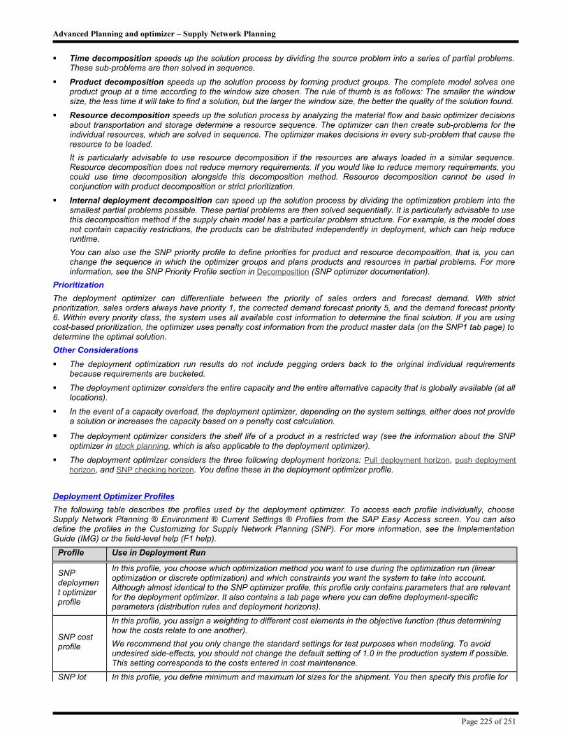
Advanced Planning and optimizer – Supply Network Planning

Time decomposition speeds up the solution process by dividing the source problem into a series of partial problems. These sub-problems are then solved in sequence.

Product decomposition speeds up the solution process by forming product groups. The complete model solves one product group at a time according to the window size chosen. The rule of thumb is as follows: The smaller the window size, the less time it will take to find a solution, but the larger the window size, the better the quality of the solution found.

Resource decomposition speeds up the solution process by analyzing the material flow and basic optimizer decisions about transportation and storage determine a resource sequence. The optimizer can then create sub-problems for the individual resources, which are solved in sequence. The optimizer makes decisions in every sub-problem that cause the resource to be loaded.

It is particularly advisable to use resource decomposition if the resources are always loaded in a similar sequence. Resource decomposition does not reduce memory requirements. If you would like to reduce memory requirements, you could use time decomposition alongside this decomposition method. Resource decomposition cannot be used in conjunction with product decomposition or strict prioritization.

Internal deployment decomposition can speed up the solution process by dividing the optimization problem into the smallest partial problems possible. These partial problems are then solved sequentially. It is particularly advisable to use this decomposition method if the supply chain model has a particular problem structure. For example, is the model does not contain capacitiy restrictions, the products can be distributed independently in deployment, which can help reduce runtime.

You can also use the SNP priority profile to define priorities for product and resource decomposition, that is, you can change the sequence in which the optimizer groups and plans products and resources in partial problems. For more information, see the SNP Priority Profile section in Decomposition (SNP optimizer documentation).

Prioritization

The deployment optimizer can differentiate between the priority of sales orders and forecast demand. With strict prioritization, sales orders always have priority 1, the corrected demand forecast priority 5, and the demand forecast priority 6. Within every priority class, the system uses all available cost information to determine the final solution. If you are using cost-based prioritization, the optimizer uses penalty cost information from the product master data (on the SNP1 tab page) to determine the optimal solution.

Other Considerations

The deployment optimization run results do not include pegging orders back to the original individual requirements because requirements are bucketed.

The deployment optimizer considers the entire capacity and the entire alternative capacity that is globally available (at all locations).

In the event of a capacity overload, the deployment optimizer, depending on the system settings, either does not provide a solution or increases the capacity based on a penalty cost calculation.

The deployment optimizer considers the shelf life of a product in a restricted way (see the information about the SNP optimizer in stock planning, which is also applicable to the deployment optimizer).

The deployment optimizer considers the three following deployment horizons: Pull deployment horizon, push deployment horizon, and SNP checking horizon. You define these in the deployment optimizer profile.

Deployment Optimizer Profiles

The following table describes the profiles used by the deployment optimizer. To access each profile individually, choose Supply Network Planning ® Environment ® Current Settings ® Profiles from the SAP Easy Access screen. You can also define the profiles in the Customizing for Supply Network Planning (SNP). For more information, see the Implementation Guide (IMG) or the field-level help (F1 help).

Profile Use in Deployment Run

SNP deployment optimizer profile

In this profile, you choose which optimization method you want to use during the optimization run (linear optimization or discrete optimization) and which constraints you want the system to take into account. Although almost identical to the SNP optimizer profile, this profile only contains parameters that are relevant for the deployment optimizer. It also contains a tab page where you can define deployment-specific parameters (distribution rules and deployment horizons).

SNP cost profile

In this profile, you assign a weighting to different cost elements in the objective function (thus determining how the costs relate to one another).

We recommend that you only change the standard settings for test purposes when modeling. To avoid undesired side-effects, you should not change the default setting of 1.0 in the production system if possible. This setting corresponds to the costs entered in cost maintenance.

SNP lot In this profile, you define minimum and maximum lot sizes for the shipment. You then specify this profile for

Page 225 of 251

Advanced Planning and optimizer – Supply Network Planning

Profile Use in Deployment Run

size profile (transportation lanes)

one specific product in the Product-Specific Means of Transport section of the transportation lane. You can thus define minimum and maximum transportation lot sizes for specific products.

If you wish to make shipments in integer multiples of a transportation lot size only, you can also define the transportation lot size as a rounding value in this profile.

To enable the deployment optimizer to take into account the minimum lot sizes and rounding values defined, you have to choose the discrete optimization method in the SNP deployment optimizer profile.

SNP optimization bound profile

If you want to perform a new planning run after a deployment optimizer planning run, you use this profile to improve planning stability by restricting possible decision variable deviations from the previous optimization plan. For example, you can permit smaller deviations at the start of the planning horizon and then increase these towards the end of the horizon to avoid too many last-minute planning changes.

Your new plan does not have to be based on the directly preceding optimization run, you can also choose earlier runs.

SNP planning profile

In this profile, you can make basic settings for the various SNP planning procedures, such as heuristic, optimizer, deployment heuristic, deployment optimizer, and Transport Load Builder (TLB).

The SNP planning profile that you activate in the SNP Customizing under Maintain Global SNP Settings applies globally for all SNP planning procedures. For some planning procedures, you can overwrite the settings of the active profile by entering another SNP planning profile during execution of planning in the background.

Parallel processing profile

You use this profile to define how background jobs are divided in parallel processes. You can specify the number of concurrent parallel processes, the number of objects per processing block, and the server group. In each case, you define the profile for one specific application function, such as the deployment optimizer.

Running Deployment Optimization

After production planning is complete and the system knows what is actually to be produced (this information is stored automatically in liveCache), the deployment optimization run generates deployment stock transfers. You can run deployment optimization in the background and in interactive Supply Network Planning.

Prerequisites

You have maintained category groups in Customizing for Supply Network Planning (Maintain Category Groups). You then have to assign these category groups to a location in the location master data (the SNP tab page). (Default settings: ATD receipts - ATI, all categories that describe demand; ATD issues - ATR, all categories that describe supply.)

Master Data Setup for the Deployment Optimizer

You have maintained the relevant deployment optimizer profiles

You have run the SNP heuristic, SNP optimizer, supply and demand propagation, or Capable-to-Match (CTM)

Procedure

To Run Deployment Optimization in the Background:

From the SAP APO Easy Access menu, choose Supply Network Planning ® Planning ® Supply Network Planning in the Background ® Deployment Optimization.

1. Enter the planning book and data view.

2. Enter an SNP planning profile that you defined in the Customizing. This contains basis settings for the SNP planning procedures. If you do not specify a profile, the system uses the default profile activated in the Customizing.

3. Enter a parallel processing profile that you defined in the Customizing for SNP. This determines how the background jobs are divided into parallel processes.

4. Enter a selection profile in which you stored your selections in interactive Supply Network Planning or manually select planning data. When selecting this data manually, enter the planning version, level ID, product (or range of products), and the location (or range of locations) that you want to plan.

5. Specify the start and end date that you want the system to consider for planning. This entry is optional. If you do not enter a start and end date, the system uses the planning buckets profile that was specified in the data view.

Enter the SNP deployment optimizer profile to be used for deployment optimizer calculations. To define a deployment optimizer profile, choose Supply Network Planning ® Environment ® Current Settings ® Profiles ® Define SNP Deployment Optimizer Profiles.

Specify the cost profile that you want to be used for deployment optimizer calculations. To maintain a cost profile, choose Supply Network Planning ® Environment ® Current Settings ® Profiles ® Define SNP Cost Profiles.

Page 226 of 251

Advanced Planning and optimizer – Supply Network Planning

6. If required, specify the optimization bound profile that you want to use for the deployment optimizer calculations. To maintain an optimization bound profile, choose Supply Network Planning ® Environment ® Current Settings ® Profiles ® Define SNP Optimization Bound Profiles. In the accompanying field, you can still specify or choose a previously executed optimization run that you want the profile specified in the Optimization Bound Profile field to reference.

7. Choose Execute.

To Run Deployment Optimization in Interactive Supply Network Planning:

From the SAP Easy Access screen, choose Supply Network Planning ® Planning ® Interactive Supply Network Planning.

1. Choose Deployment Optimizer. The Deployment Optimizer window appears. The pushbutton for accessing the deployment optimizer is displayed on the interactive desktop automatically if you are using the standard SNP planning book SNP94. However, if you create your own planning books and wish to use the deployment optimizer in interactive planning, you must specify that you want this pushbutton to be displayed. You do this in the Design mode of the interactive planning desktop.

2. On the Optimization tab page in the Deployment Optimizer window, you can choose one of your predefined deployment

optimizer profiles, cost profiles, and optimization bound profiles. By choosing the icons , , and , you branch to the maintenance screens for the deployment optimizer profiles, cost profiles, and optimization bound profiles to make changes to existing profiles, for example.

3. Choose to start the optimization run.

The current solution resulting costs determined by the optimizer are displayed in the Current Solution area of the Optimization tab page. The individual steps of the optimization process are displayed in the Status area during the optimization run and information about intermediary solutions is displayed in the Solution Run area. In addition to this, messages about the current optimization run are displayed in the Messages area.

You can also display the products that were selected for this optimization run by choosing . Choose to branch to the Supply Network Planning: Optimizer log file screen. From there, you can decide which type/form of log to display (the message log, input log, or results in a text file for example.)

4. Choose the Solutions tab page to view information about the previous optimization runs. If you select a solution in the right-hand screen area, the data corresponding to that solution appears in the left-hand area.

5. Choose the Messages tab page to view messages about the previous optimization runs. If you select an optimization run in the left-hand screen area, the messages corresponding to that optimization run appear in the right-hand area.

Result

After the deployment optimization run, the system automatically converts SNP stock transfers into deployment stock transfers, which are used for transportation planning in the Transport Load Builder (TLB).

Automatic Cost Generation

Costs play an essential role for optimization-based planning in Supply Network Planning (SNP). The optimizer selects the plan with the lowest total costs from all the permitted production and distribution plans. This means that the optimizer also makes business decisions based on the costs involved for covering a demand at a certain point in time, for example.

You can provide the optimizer with the costs for planning by specifying your actual costs such as production and transportation costs in the system. You can also define control costs that are in accordance with your business goals. For the planner, however, the conversion of business goals into control costs is not easy.

With the automatic cost generation function, you can easily generate all the control costs relevant to the optimizer (that is, the cost model). The system generates these costs automatically based on the business goals you have defined. The system requires the main goal to be the maximization of the service level. You can also define the following goals:

Consideration of demand and product priorities

Consideration of procurement priorities

In addition, you can use this function to quickly and easily create an optimization-based production plan. To create a finite (capacity-based) production plan, you only have to make a few additional settings (such as the consideration of capacities).

Features

Generating the Cost Model

The system generates the following control costs:

Storage costs

Production costs, that is, costs of the production model (PPM) or of the production data structure (PDS).

Product-specific transportation costs

Procurement costs

Penalty costs for shortfall of safety stock

Page 227 of 251

Advanced Planning and optimizer – Supply Network Planning

Penalty costs for non-delivery

Penalty costs for late delivery

In order for the system to be able to calculate the costs for a late delivery, you must define a maximum delay in the product master data on the SNP 1 tab page.

The system ignores all the costs you may have defined in the master data. They remain unchanged in the system even after cost generation, however.

The system does not generate the following costs, because it would require additional information from the planner or because the costs are only relevant to complex scenarios:

Cost functions (production, shipment, procurement)

Costs for means of transport

Costs for the use of the available capacity of resources (costs for using the normal and maximum available capacities or for falling short of the minimum available capacity)

In addition, the system does not consider the cost profile for weighting costs that you can define for optimization-based planning.

Properties of the Generated Cost Model

The system ensures the following properties of the generated cost model:

The model has no anomalies.

The system defines the costs such that undesired effects do not arise, such as:

Not covering a demand due to too low penalties costs for non-delivery

Planning a shipment due to too low costs at the destination location

Planning a shipment to save storage costs

The system also covers the demands as timely as possible.

The model is stable.

The costs are, for example, independent of period length and transaction data.

The model is coherent.

For example, the transportation costs increase proportionally to the shipment length and the product value increases with the depth of production.

The system automatically uses the value 1 for the value of raw products (products without input products). If you want the system to base the calculation of the product value on the actual storage costs, you can make this setting in the SNP or deployment optimizer profiles on the Automatic Cost Generation tab page.

The system cannot guarantee this model property, because the first two properties have higher priority and it is not always possible to guarantee all three.

The generated cost model is independent from the costs defined in the master data (except for possible consideration of storage costs). The system does not support a combination of these two cost models (for example, completion of the master data cost model).

Definition of the Business Goals

The system calculates the costs based on the business goals you have defined. For further information see Definition of the Business Goals.

Actions

1. Define your goals for optimization-based planning as described.

2. If, for example, you want to create a finite (capacity-based) plan, set the corresponding indicator for the consideration of capacity restrictions on the General Restrictions tab page of the SNP or deployment optimizer profile.

3. Set the Automatic Cost Generation indicator in the SNP or deployment optimizer profile.

4. Execute an SNP or deployment optimization run. For more information, see Running the Optimizer in the Background,

Running the Optimizer from the Interactive Planning Desktop, or Running Deployment Optimization.

5. Display the application log that is in the Results Log section and contains information about the generated costs. For more information about optimization logs, see Application Logs for Optimizers.

Page 228 of 251

Advanced Planning and optimizer – Supply Network Planning

Definition of the Business Goals

If you want to create an optimization-based production plan with the automatic cost generation function, first define your business goals for planning. The system then uses these goals to automatically generate the corresponding control costs, based on which the optimizer makes planning decisions.

The main goal of planning is to maximize the service level. You can also define the following additional goals:

Consideration of demand and product priorities

Consideration of procurement priorities

You define these goals in the SNP or deployment optimizer profile on the Automatic Cost Generation tab page.

Features

Consideration of demand and product priorities

You can define priorities for three different priority classes of the demand and the safety stock:

Customer demand

Corrected demand forecast

Demand forecast

Safety stock

The standard setting is that all priority classes and the safety stock have the same priority.

In addition, you can define that the system also considers the priority of products. You can enter this priority in the master data of the location product on the SNP 2 tab page. The system considers the product priority in combination with the demand priority. You can define which priority is more important and is to be considered by the system first.

To simplify this combination of both priority types, you must also subdivide the product priorities into three classes of A, B, and C products.

The following figure shows exactly how the system proceeds if the demand priority is more important than the product priority or vice versa:

Consideration of procurement priorities

You can define that the system considers the procurement priorities of production process models (PPMs) or production data structures (PDS) as well as transportation lanes. You define this priority in the master data of the PPMs/PDS and transportation lanes (specific to the product). The procurement priority of sources of supply for in-house production is always more important than the priority of sources of supply for external procurement (same as the SNP heuristic procedure).

The system always tries to first cover all the demand of a period with receipts from all the sources of supply available in this period (in the sequence of the procurement priority of these sources of supply). Only after this does it try to cover the demand with receipts from sources of supply from an earlier period. If the system has to switch to an earlier or later period, it may not be able to follow this principle in this period.

Costs Maintenance

Costs play an essential role for optimization-based planning in Supply Network Planning (SNP). The optimizer selects the plan with the lowest total costs from all the permitted production plans.

Use this function to define all costs used by the optimizer and assigned to the master data from a single point of access. The master data is then automatically updated for the selected planning version.

Page 229 of 251

Advanced Planning and optimizer – Supply Network Planning

To call the function, on the SAP Easy Access screen, choose Advanced Planning and Optimization →Master Data ® Application-Specific Master Data® Supply Network Planning ® Maintain Costs(Directory) or Maintain Costs (Table).

Features

You can define the following costs:

Production costs

Storage costs

Handling costs

Transportation costs

Procurement costs

Costs for late delivery

Costs for non-delivery

Costs for using the available capacity of resources

Cost functions

Application Logs for Optimizers

When you execute an optimization-based planning function in Supply Network Planning (SNP) in the background (mass processing), the system automatically generates an application log. Amongst other things, this log contains planning results, such as planned orders and stock transfers created, as well as error, warning, and information messages. The input data for the optimization run and the costs of the solution determined by the optimizer are also displayed, for example.

The central Optimizer Log Data function is available for accessing optimization run logs. From the SAP Easy Access screen, choose Advanced Planning and Optimization ® Supply Network Planning ® Reporting ®Optimizer Log Data. You can use this function to access the following SNP planning functions:

SNP Optimizer

Deployment Optimizer

Capacity Leveling (optimization-based method)

Sourcing of Forecast

Features

The Optimizer Log Data function provides an overview of the generated logs. Amongst other things, the list of logs contains the following data:

Log status

A traffic light or flag indicates whether the optimization run is still in progress, has already ended, or was terminated with a message (see F1 help).

Log creator

Optimizer profile used

Start and finish time of the run

Runtimes of the individual optimization steps

An optimization run has three steps (data reading, model consistency check, and solution calculation, as well as order creation).

Total costs of solution

Log expiration date

You specify the log expiration date globally for all optimization logs in Customizing for Advanced Planning and Optimization (APO) under Basis Settings → Optimization ® Basic Functions ® Maintain Global Settings. However,

you can also change this date for one specific optimization run by choosing Change Expiration Date. The log is automatically deleted after the expiration date if you execute the /SAPAPO/OM_REORG_DAILY report.

You can also delete the log from the list, set filters and sort entries.

If you double click a log or choose Display Log, you receive the following data and sub-logs for the log.

Input Parameter - Contains the settings that you made on the initial screen for the planning function.

Location Products - Contains the location products selected for the optimization run.

Page 230 of 251

Advanced Planning and optimizer – Supply Network Planning

Deletion Time Period - Specifies a time period in which the system deletes existing planned orders and stock transfers before actual optimization.

Input Log - Contains the input data considered by the system during the optimization run (that is, master data and transaction data). The data is divided into a number of tables (such as ET_LOCMAT). You can display the content of these tables on the right-hand side of the screen. For more information, see Optimization Input Log.

Results Log - Contains all results of the optimization run, such as planned orders, stock transfers, resource consumption, costs, and penalty costs. The data is divided into a number of tables (such as ET_PROMO). You can display the content of these tables on the right-hand side of the screen.

Result Indicators - Contains indicators that display the quality of the optimization solution, such as service level and shortfall of safety stock. For more information, see Result Indicators.

Explanations - Contains the results of an explanation tool run (see below).

Extended Results Log - In this log, you can display the results of the optimization run in the interactive SNP planning form.

Message Log - Contains error messages, warning messages, and information messages generated by the system during the optimization run. They are ordered according to meaning, that is, whether they refer to the optimization run settings or to the three main steps of the run.

Trace File - All individual optimization run steps are logged in this text file. It is saved on the optimization server, but you can also download it to your own computer.

Costs - Contains detailed information about the costs of the solution determined by the optimizer. For more information, see Resulting Costs of Optimization.

Solution Quality - Contains the costs of the best solution determined by the optimizer up to the time displayed. If you used a decomposition method, you can also relate the costs the partial problem solved up to this time.

You can use the log to determine whether you can reduce the optimizer runtime without effecting solution quality.

Note that the input log and the results log, as well as the deletion time period, are only displayed if you have set the Write All Log Data indicator in the optimizer profile being used. Even if an error occurred in the first step of the optimization run (data reading), the log may not be available.

You can also download the input log and the results log to your own computer. To do this, choose Download Input

Log or Download Results Log. The logs are then saved in RELATIOM text format.

If you select a log and choose Explain, you go to the Explanations of SNP Optimization Resultsscreen. From this screen you can execute the explanation tool which explains two important exceptional situations of an optimization run: non-deliveries and shortfall of safety stock.

Monitoring TLB and Deployment Alerts

You can use the Alert Monitor to monitor alerts for the Transport Load Builder and for Deployment. To do this, you define a TLB alert profile containing a user-specific selection of alerts that are relevant for your planning area.

Features

The following table shows you the alert types available, and a brief description of each one.

For all the alerts except Invalid Delivery Date, you can enter priority variants based on critical values.

TLB/deployment alerts Description

Fair share (general)

The fair share percentage is determined according to the rule specified in the deployment heuristic profile (SNP2 tab in the location product master). The system triggers this alert if the percentages to deploy in order to meet product demand fall below the percentages specified in the master data.

Fair share (customers only)

Same as above, except in this case fair share distribution refers only to customers instead of locations. (for example, VMI customers)

Invalid shipmentWhen the shipment does not fulfill the parameters for the capacity of the means of transport

(such as volume, weight, and pallet positions) defined in the TLB profile, the system generates an alert.

Invalid delivery dates You active this alert using the /SAPAPO/TLB_CHK_DATE BAdI.

Activities

1. Select the alert types that are relevant to you, and define threshold values where required.

2. Select the objects (products, transportation lanes, means of transport) for which the system should determine alerts.

Page 231 of 251

Advanced Planning and optimizer – Supply Network Planning

3. If necessary, assign the TLB alert profile to your Overall Alert Profile, your SCC User Profile , or your user by selecting Advance Planning and Optimization ® Supply Network Planning ® Environment ® Current Settings ® Assign Planners to Alert Profiles from the SAP Easy Access screen.

For performance reasons, we recommend restricting the number of alerts to be displayed to a minimum.

Transport Load Builder

You can use the Transport Load Builder (TLB) to group transport loads for certain means of transport whilst ensuring that the capacity of the means of transport is utilized as much as possible. The main aims of TLB planning are:

Building of transport loads that are within the parameter limits defined by the user (such as weight and volume)

Straight loading or load balancing of means of transport

The TLB groups deployment stock transfers or replenishment orders that were generated for individual products in the previous planning runs, into TLB shipments for several products.

You can use the TLB in the SAP Inventory Collaboration Hub (SAP ICH) or in Supply Network Planning (SNP). In SAP ICH, there are additional functions available. These are features that are not available in the SNP TLB. For more information, see Additional TLB Functions in SAP ICH.

You have set up the master data for the TLB. For more information, see Master Data Setup for the Transport Load Builder.

You have defined upper and lower limits for the TLB parameters in a TLB profile, and have assigned this profile to the means of transport in the transportation lane. To create the TLB profile, proceed as follows:

SAP ICH: In the SAP ICH Web Application menu, choose Transport Load Builder → Profiles and Rules.

SNP: On the SAP Easy Access screen, choose Advanced Planning and Optimization →Supply Network Planning → Environment ® Current Settings ® Profiles® Define Profiles for Transport Load Builder (TLB).

For more information, see TLB Profile.

You have defined a profile for the TLB basic settings in Customizing for SAP ICH or SNP. If you do not define a profile, the TLB uses the default settings. To create the profile, proceed as follows:

SAP ICH: In Customizing for SAP ICH, choose Customer Collaboration → Transport Load Builder → Make TLB-Basic Settings.

SNP: In Customizing for SNP, choose Basic Settings → Make TLB Basic Settings.

For more information, see the Implementation Guide (IMG).

If you are using SNP, you can make settings for the layout of interactive TLB planning in SNP in Customizing for SNP under Basic Settings → Change Display of Parameters in Interactive TLB. For more information, see the IMG.

If you want the TLB to be able to load a pallet with several different products, you can set the TLB: Pallet Loading parameter to Product Mix in Customizing for SNP under Maintain Global SNP Settings. If you do not make this setting, the SNP TLB is permitted to load pallets with products of the same type only.

If you are using SAP ICH, you must make additional settings for the TLB. For more information, see Additional TLB Functions in SAP ICH.

Features: Building of Transport Loads

The TLB first groups deployment stock transfers or replenishment orders from the current period into TLB shipments. In doing so, the TLB tries to load the shipments as far as possible to the upper parameter limits that you defined in the TLB profile for that means of transport.

The TLB also considers the loading method that you defined for the means of transport in the transportation lane. As far as possible, the TLB loads the transport loads with the same products, or products from the same loading group (straight loading), or distributes the products evenly amongst all transport loads built (load balancing). Do note, however, that the TLB does not use optimization methods and can, therefore, not guarantee the optimal solution. The TLB considers the individual loading methods as follows:

Straight loading: The TLB sorts the loading groups and then the products within the loading group alphabetically. In the second step, the TLB distributes the loading groups and products into shipments, in the sequence in which they were sorted.

If a loading group can only be partially loaded onto a shipment, the TLB loads the rest of the loading group onto the next shipment. In this way, it is possible for a loading group to be too large or too small for a shipment.

Load balancing: The TLB tries to distribute products to shipments in such a way, that the product percentages are, as far as possible, the same for every shipment.

Page 232 of 251

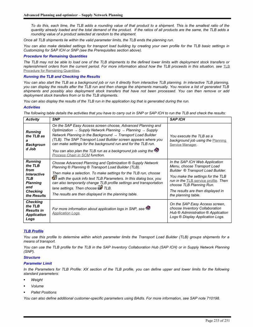
Advanced Planning and optimizer – Supply Network Planning

To do this, each time, the TLB adds a rounding value of that product to a shipment. This is the smallest ratio of the quantity already loaded and the total demand of the product. If the ratios of all products are the same, the TLB adds a rounding value of a product selected at random to the shipment.

Once all TLB shipments lie within the valid parameter limits, the TLB ends the planning run.

You can also make detailed settings for transport load building by creating your own profile for the TLB basic settings in Customizing for SAP ICH or SNP (see the Prerequisites section above).

Procedure for Remaining Quantities

The TLB may not be able to load one of the TLB shipments to the defined lower limits with deployment stock transfers or replenishment orders from the current period. For more information about how the TLB proceeds in this situation, see TLB Procedure for Remaining Quantities.

Running the TLB and Checking the Results

You can also start the TLB as a background job or run it directly from interactive TLB planning. In interactive TLB planning, you can display the results after the TLB run and then change the shipments manually. You receive a list of generated TLB shipments and possibly also deployment stock transfers that have not been processed. You can then remove or add deployment stock transfers from or to the TLB shipments.

You can also display the results of the TLB run in the application log that is generated during the run.

Activities

The following table details the activities that you have to carry out in SNP or SAP ICH to run the TLB and check the results:

Activity SNP SAP ICH

Running the TLB as a Background Job

On the SAP Easy Access screen choose, Advanced Planning and Optimization → Supply Network Planning → Planning → Supply Network Planning in the Background → Transport Load Builder (TLB). The SNP Transport Load Builder screen appears where you can make settings for the background run and for the TLB run.

You can also plan the TLB run as a background job using the Process Chain in SCM function.

You execute the TLB as a background job using the Planning Service Manager.

Running the TLB from Interactive TLB Planning and Checking the Results

Choose Advanced Planning and Optimization ® Supply Network Planning ® Planning ® Transport Load Builder (TLB).

Then make a selection. To make settings for the TLB run, choose

with the quick info text TLB Parameters. In this dialog box, you can also temporarily change TLB profile settings and transportation

lane settings. Then choose TLB.

The results are then displayed in the planning table.

In the SAP ICH Web Application Menu, choose Transport Load Builder ® Transport Load Builder.

You make the settings for the TLB run in the TLB service profile. Then choose TLB Planning Run.

The results are then displayed in the planning table.

Checking the TLB Results in Application Logs

For more information about application logs in SNP, see Application Logs.

On the SAP Easy Access screen, choose Inventory Collaboration Hub ® Administration ® Application Logs ® Display Application Logs.

TLB Profile

You use this profile to determine within which parameter limits the Transport Load Builder (TLB) groups shipments for a means of transport.

You can use the TLB profile for the TLB in the SAP Inventory Collaboration Hub (SAP ICH) or in Supply Network Planning (SNP).

Structure

Parameter Limit

In the Parameters for TLB Profile: XX section of the TLB profile, you can define upper and lower limits for the following standard parameters:

Weight

Volume

Pallet Positions

You can also define additional customer-specific parameters using BAdIs. For more information, see SAP note 710198.

Page 233 of 251

Advanced Planning and optimizer – Supply Network Planning

Rule Relationships

In the TLB profile section, you can define very flexible rule relationships for linking upper and lower limits. The following standard connections are available:

Connect upper limits with 'and', lower limits with ‘or’. When building transport loads, the TLB may not exceed any of the upper limits defined. One lower limits must also be reached or exceeded, depending on how you have defined the rules.

Connect upper limits with 'and', lower limits with ‘and’. The TLB may not exceed any of the upper limits defined. All lower limits must be reached or exceeded.

If you have chosen the '=' operator, the TLB also interprets the lower limits as upper limits.

In addition to the standard connection, you can also define user-specific relationships between the rules. Using the AND and OR operators as well as brackets, you can determine which combinations of rules you want the TLB to use when building transport loads.

When processing the rules, the TLB always considers the AND connection first and then the OR connection. If you want to change this sequence, you can put the OR connection in brackets.

You have defined specific upper and lower limits for the parameters: Weight (Rule 1), Volume (Rule 2), and Pallet Positions (Rule 3). You now want to specifiy that you want either both rules 1 and 2, or rule 3 to be fulfilled. You then enter 1 AND 2 OR 3 in the Rule Details field.

If you want to define a rule connection, such as 1 OR 2 AND 3 and also want the TLB to consider the rules in this sequence, you must define the rules as follows: (1 OR 2) AND 3.

TLB Procedures for Remaining Quantities

If the Transport Load Builder (TLB) has not been able to load one of the TLB shipments to the upper limits defined with the deployment stock transfers or replenishment orders of the current period, the TLB first redistributes product quantities. The TLB tries to ensure that all shipments lie within the valid upper and lower parameter limits by only loading some shipments to the defined lower limits. To do this, the TLB rebuilds all transport loads, taking the loading method into account.

If the TLB does not produce a valid solution this way either, it uses the following shipment sizing methods.

Shipment Upsizing

Shipment Downsizing

Features

Shipment Upsizing

The TLB upsize the product quantities to be transported by including further deployment stock transfers or replenishment orders that lie within the pull-in horizon. The TLB also sorts the stock transfers within this horizon according to their days’ supply.

You can also define a coverage period for a product in the master data for location product. The TLB is then only allowed to bring forward as many products that are necessary to cover demand within this time period. You can also rule our shipment upsizing for a product.

The TLB system upsize the shipment quantities with individual rounding values of the product until all shipments lie within the valid upper and lower parameter limits.

Shipment Downsizing

Taking days’ supply into account, the TLB downsizes the product quantities to be transported by prioritizing and reducing deployment stock transfers or replenishment orders in the current period.

Shipment Upsizing or Downsizing Decision

The TLB decides whether the to upsize or downsize a shipment based on a threshold value and a decision basis for shipment sizing. In the SAP Inventory Collaboration Hub (SAP ICH), the TLB can also make the decision based on costs.

You make these settings in the transportation lane for the means of transport. For more information, see Master Data Setup for the Transport Load Builder.

Detailed Setting

You can also make detailed settings for shipment sizing by creating your own profile for the TLB basic settings in the SAP ICH, or Supply Network Planning (SNP) Customizing (see Prerequisites section under Transport Load Builder). For example, for shipment upsizing, you can specify that you want the shipments to be loaded, as far as possible, to the upper parameter limit.

Page 234 of 251

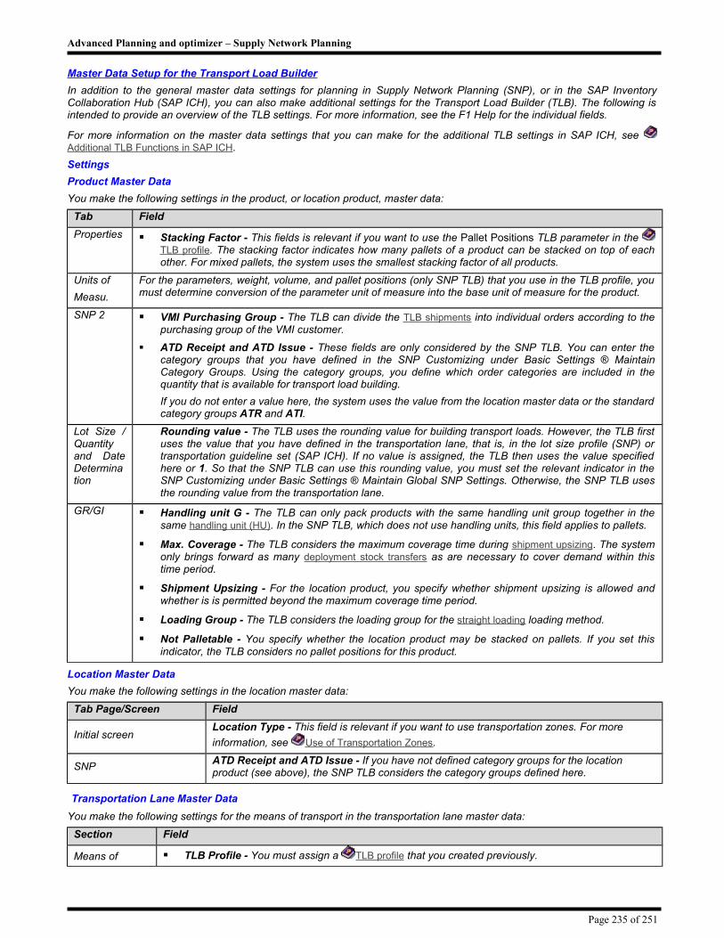
Advanced Planning and optimizer – Supply Network Planning

Master Data Setup for the Transport Load Builder

In addition to the general master data settings for planning in Supply Network Planning (SNP), or in the SAP Inventory Collaboration Hub (SAP ICH), you can also make additional settings for the Transport Load Builder (TLB). The following is intended to provide an overview of the TLB settings. For more information, see the F1 Help for the individual fields.

For more information on the master data settings that you can make for the additional TLB settings in SAP ICH, see Additional TLB Functions in SAP ICH.

Settings

Product Master Data

You make the following settings in the product, or location product, master data:

Tab Field

Properties Stacking Factor - This fields is relevant if you want to use the Pallet Positions TLB parameter in the TLB profile. The stacking factor indicates how many pallets of a product can be stacked on top of each other. For mixed pallets, the system uses the smallest stacking factor of all products.

Units of

Measu.

For the parameters, weight, volume, and pallet positions (only SNP TLB) that you use in the TLB profile, you must determine conversion of the parameter unit of measure into the base unit of measure for the product.

SNP 2 VMI Purchasing Group - The TLB can divide the TLB shipments into individual orders according to the purchasing group of the VMI customer.

ATD Receipt and ATD Issue - These fields are only considered by the SNP TLB. You can enter the category groups that you have defined in the SNP Customizing under Basic Settings ® Maintain Category Groups. Using the category groups, you define which order categories are included in the quantity that is available for transport load building.

If you do not enter a value here, the system uses the value from the location master data or the standard category groups ATR and ATI.

Lot Size / Quantity and Date Determination

Rounding value - The TLB uses the rounding value for building transport loads. However, the TLB first uses the value that you have defined in the transportation lane, that is, in the lot size profile (SNP) or transportation guideline set (SAP ICH). If no value is assigned, the TLB then uses the value specified here or 1. So that the SNP TLB can use this rounding value, you must set the relevant indicator in the SNP Customizing under Basic Settings ® Maintain Global SNP Settings. Otherwise, the SNP TLB uses the rounding value from the transportation lane.

GR/GI Handling unit G - The TLB can only pack products with the same handling unit group together in the same handling unit (HU). In the SNP TLB, which does not use handling units, this field applies to pallets.

Max. Coverage - The TLB considers the maximum coverage time during shipment upsizing. The system only brings forward as many deployment stock transfers as are necessary to cover demand within this time period.

Shipment Upsizing - For the location product, you specify whether shipment upsizing is allowed and whether is is permitted beyond the maximum coverage time period.

Loading Group - The TLB considers the loading group for the straight loading loading method.

Not Palletable - You specify whether the location product may be stacked on pallets. If you set this indicator, the TLB considers no pallet positions for this product.

Location Master Data

You make the following settings in the location master data:

Tab Page/Screen Field

Initial screenLocation Type - This field is relevant if you want to use transportation zones. For more

information, see Use of Transportation Zones.

SNPATD Receipt and ATD Issue - If you have not defined category groups for the location product (see above), the SNP TLB considers the category groups defined here.

Transportation Lane Master Data

You make the following settings for the means of transport in the transportation lane master data:

Section Field

Means of TLB Profile - You must assign a TLB profile that you created previously.

Page 235 of 251

Advanced Planning and optimizer – Supply Network Planning

Transport

Loading Method - You specify whether you want the TLB to consider the straight loading oder load balancing loading method.

Pull-In Horizon - If the TLB carries out a shipment upsizing, it considers the pull-in horizon.

Siz.Desn and Shpmt Thr.Val. - In the Siz.Decsn field, you determine how the TLB calculates the value it uses to decide about shipment sizing. The system compares the base value calculated with the value you have entered in the Shpmt Thr.Val field, and then carries out shipment upsizing or downsizing.

Product-specific transportation

T. Lot Prfl - This field is only considered by the SNP TLB. You can enter a profile here that you created in the SNP Customizing under Basic Settings ® Profiles ® SNP-Lot Size Profile (Transportation Lane). The TLB considers the value defined in this profile (see above).

Use of Transportation Zones

In the Transport Load Builder (TLB), you can use transportation zones to group several locations together in one group (that is, one zone) and use one means of transport to ship TLB shipments to multiple locations. The system regards TLB shipments for multiple locations as one shipment for one location.

Activities

If you want to use transportation zones, create a location as location type 1005 (transportation zone) or 1006 (stock transfer point)in the location master data for the Cross-Docking scenario in the SAP Inventory Collaboration Hub (SAP ICH)).

After creating the location (type transportation zone or stock transfer point), assign the relevant location in the hierarchy master data for transportation zones (select Master Data → Hierarchy). You can display location hierarchies in the shuffler for interactive TLB planning.

In addition, you must create a transportation lane that has this transportation zone as its destination or source location, and the same destination or source locations as the locations contained within this transportation zone.

In this instance, the TLB only considers the deployment stock transfers or the replenishment orders of locations you have assigned to the transportation zone.

Monitoring TLB and Deployment Alerts

You can use the Alert Monitor to monitor alerts for the Transport Load Builder and for Deployment. To do this, you define an TLB alert profile containing a user-specific selection of alerts that are relevant for your planning area.

Features

The following table shows you the alert types available, and a brief description of each one.

For all the alerts except Invalid Delivery Date, you can enter priority variants based on critical values.

TLB/deployment alerts Description

Fair share (general)

The fair share percentage is determined according to the rule specified in the deployment heuristic profile (SNP2 tab in the location product master). The system triggers this alert if the percentages to deploy in order to meet product demand fall below the percentages specified in the master data.

Fair share (customers only)

Same as above, except in this case fair share distribution refers only to customers instead of locations. (for example, VMI customers)

Invalid shipmentWhen the shipment does not fulfill the parameters for the capacity of the means of transport

(such as volume, weight, and pallet positions) defined in the TLB profile, the system generates an alert.

Invalid delivery dates You active this alert using the /SAPAPO/TLB_CHK_DATE BAdI.

Activities

1. Select the alert types that are relevant to you, and define threshold values where required.

2. Select the objects (products, transportation lanes, means of transport) for which the system should determine alerts.

3. If necessary, assign the TLB alert profile to your Overall Alert Profile, your SCC User Profile , or your user by selecting Advance Planning and Optimization ® Supply Network Planning ® Environment ® Current Settings ® Assign Planners to Alert Profiles from the SAP Easy Access screen.

For performance reasons, we recommend restricting the number of alerts to be displayed to a minimum.

Page 236 of 251

Advanced Planning and optimizer – Supply Network Planning

Prioritization of Deployment Stock Transfers

The Transport Load Builder (TLB) uses the results of the deployment run (deployment stock transfers) to create TLB shipments for multiple products to optimize the loading of means of transport. It takes into account the constraints defined in the TLB profile, such as weight and volume. When the TLB upsizes or down sizes shipments, it prioritizes deployment stock transfers according to their days’ supply.

You can use the function for prioritizing stock transfers to separate deployment transfers according to demand type, and then assign priorities to the resulting stock transfers. You can then also use these shipment priorities for manual transport load building, in order to ensure that the important product quantities are given priority during loading.

The TLB does not consider shipment priority during a TLB run.

Integration

You can prioritize only those deployment stock transfers not to be transferred to a connected OLTP system or those to be transferred as purchase requisitions. You cannot use this function to process deployment stock transfers that are to be transferred to the OLTP system as purchase orders (see also the Prerequisites).

Prerequisites

The prerequisites for deployment stock transfer prioritization are much the same as those for performing a deployment run. It is essential that the relevant transportation lanes and products are valid. Note that the prioritization function only takes into account the rounding value that you specified at the transportation lane or in the location product master (first, the value from the transportation lane and, if this does not exist, then the value from the product master); it does not consider the rounding profile, nor does it consider maximum or minimum lot sizes. For more information, see Running the Deployment Heuristic or Running Deployment Optimization.

The following prerequisites also apply:

In Customizing for Supply Network Planning (SNP), you have set (in Configure Transfer to OLTP Systems) that the deployment stock transfers you want to prioritize are not to be transferred to a connected OLTP system or are to be transferred as purchase requisitions.

You have performed a deployment run that has created deployment stock transfers.

Features

Shipment Priority Calculation

The deployment stock transfer prioritization function first splits the quantity of one deployment stock transfer into a maximum of three new deployment stock transfers according to the following categories:

Category 1: Stock transfers for fulfilling current demands and shortages

Category 2: Stock transfers for fulfilling demands based on a predefined target stock level

Category 3: Stock transfers representing a surplus delivery that exceeds the target stock level (based on push deployment, for instance)

The original deployment stock transfer is deleted after this splitting.

The system then assigns a priority to the new deployment stock transfers. There is a specific range of priorities available for each category. The system makes another weighting within this priority range. The assigned shipment priority then indicates the relative significance of the deployment stock transfer (or product quantity) in terms of demand fulfillment. The following table illustrates how the priorities are calculated:

Shipment Priority Calculation

Category: Priority range Formula

Cat1: Current demands and shortages 0 Cat1-Prio. = 0

Cat2: Demands based on the target stock level 1 - 10 Cat2-Prio. = Av.Stock/TgtStock*10

Cat3: Surplus delivery exceeding the target stock level 11 – 99 Cat3-Prio = 10 + T(Cat3)/TgtStock*10

Key to the table:

Av.Stock = Available stock at the destination location before current demands and shortages at the destination location have been fulfilled

TgtStock = Target stock level

T(Catx) = Quantity of the respective category

In the priority range of category 2, the priority indicates what proportion of the target stock level was already covered before the stock transfer was received. A small proportion indicates a high stock transfer priority (small priority number).

Page 237 of 251

Advanced Planning and optimizer – Supply Network Planning

In the priority range of category 3, the priority indicates how much surplus stock the stock transfer is to provide above the target stock level. The higher the surplus stock, the lower the priority of the stock transfer (large priority number).

Use of the Shipment Priority

The shipment priority assigned to the deployment stock transfer is displayed for you in the TLB view of interactive Supply Network Planning. You can use the priority to estimate the relative significance of a stock transfer and uses this information when manually creating TLB shipments.

Simulation and Logs

You can specify whether you want the prioritization results to be saved immediately or displayed only for simulation purposes. If you decide to save them immediately, the deployment stock transfers are created in liveCache.

If you run the function for prioritizing deployment stock transfers directly, a results log is automatically displayed showing a list of the deployment stock transfers that have been created. If you run the function in the background, you can access the results in the spool list. You can also display an error log. To do this, choose Display Logs.

Activities

1. Perform a deployment run. For more information, see Running the Deployment Heuristic or Running Deployment Optimization.

2. Access the deployment stock transfer prioritization function from the SAP Easy Access screen (Supply Network Planning ® Planning ® Supply Network Planning in the Background ® Prioritize Deployment Stock Transfers).

3. Make the relevant settings. You define the following parameters:

Prioritization horizon: You specify the number of days over which the system is to take deployment stock transfers into account for prioritization. If you run the function directly, the time period starts from today’s date; if you run it in the background, it starts from the date specified for the run.

Destination Locations: You can restrict prioritization of deployment stock transfers to specific destination locations. If you do not specify a location, the system runs prioritization for all the destination locations.

Fix Deployment Stock Transfers: You can specify that you want all deployment stock transfers that were created after prioritization to be fixed (which means they cannot be changed in any subsequent planning runs). Deployment stock transfers that had previously been fixed are split independently of the setting made in this field and then re-fixed.

4. You run the function. The result of this a list of the newly created deployment stock transfers with assigned priorities. Each original deployment stock transfer can be split into a maximum of three new deployment stock transfers.

5. You can build transport loads manually in interactive TLB planning (after a TLB run, if necessary). Select Advanced Planning and Optimization ® Supply Network Planning ® Planning ® Transport Load Builder (TLB) from the SAP Easy Access screen.

Source Determination in Supply Network Planning

The individual planning procedures in Supply Network Planning (SNP) have very different source determination methods. While the SNP heuristic uses quota arrangements and procurement priorities as a basis for choosing the source of supply, the SNP optimizer bases its source determination decisions on costs. Deployment, on the other hand, uses source determination not to determine sources of supply but instead to determine the destination locations to which product stock is to be distributed.

Features

SNP Heuristic

The heuristic determines the sources of supply as follows:

1. The system first takes into account the defined quota arrangements.

2. If there are no quota arrangements available, the procurement priority specified in the Production Process Model (PPM), in the Production Data Structure (PDS), or in the transportation lane is used.

3. If both quota arrangements and procurement priorities have been defined, the system uses the quota arrangements.

4. If neither quota arrangements nor procurement priorities exist, the system chooses the most cost-efficient source of supply.

5. If all sources of supply have the same costs, the general guidelines for source determination apply (see Determination of Source of Supply Ranking List).

If there is neither a valid transportation lane (for procurement type F; external procurement) nor valid PPM/PDS (for procurement type E; in-house production), the system creates an SNP stock transfer or SNP planned order with no reference to a source of supply. The same applies if there is no product in the source location of the transportation lane.

Page 238 of 251

Advanced Planning and optimizer – Supply Network Planning

SNP Optimizer

Since the SNP optimizer basically determines the most cost-efficient solution, its sourcing decisions are also cost-based, which means the optimizer does not take into account quota arrangements or procurement priorities.

This also means that you can only influence source determination or, to a certain extent, prioritize sources by specifying costs. For example, you can use production costs to prioritize production resources and transportation costs to prioritize the procurement location. Note however, that the optimizer always takes all influencing factors into account (such as storage costs).

If there is no valid transportation lane for procurement type F (external procurement), the system creates an SNP stock transfer with no reference to a source of supply. If there is no valid PPM/PDS for procurement type E (in-house production), the system’s behavior is governed by whether or not the SNP: No Planned Order indicator has been set in the planning version. If this indicator is set, the SNP optimizer does not create any planned orders; if it is not set, the SNP optimizer creates planned orders with no reference to a PPM/PDS.

For more information, see Source Determination (Optimizer).

Deployment

Deployment determines the destination locations to which the product stock is to be distributed. Therefore, deployment only considers transportation lanes as "sources."

Deployment Heuristic

In the deployment heuristic, it is cruicial that the corresponding transportation lanes and one of the means of transport assigned to it are valid in the planning time period. The system first determines all valid means of transport for every individual period and every target location, and then decides which means of transport to use to create the deployment stock transfers. Generally, the system tries to orientate itself on the results of the SNP run and adopt the SNP-stock transfers created there. If there a multiple means of transport, or if there are no SNP stock transfers in a period, the system chooses the means of transport with the shortest mover time. If no valid transportation lanes or means of transport are available, the system cannot create any deployment stock transfers.

Deployment uses distribution rules to decide which product stock proportions are to be distributed to the different destination locations; for example, it uses fair share rules in the event of a supply surplus or push rules if there is insufficient supply to fulfill demand. These rules are based partly on quota arrangements or priorities (distribution priority in the transportation lane).

Deployment Optimizer

The deployment optimizer generally decides which source locations to distribute available product stock to and which means of transport to use, based on the lowest total costs and by considering all restrictions (such as transport capacity) In doing so, the system may also take detours into consideration.

The deployment optimizer also decides which proportion of product stock is distributed to which source location based on the distribution rules.

Capacity Leveling

Capacity leveling performs a source determination if the system decides to switch the source of supply. If the chosen leveling procedure is heuristic-based, sources are determined in the same way as for the SNP heuristic, if optimizer-based, source determination corresponds to that of the SNP optimizer. However, with optimizer-based capacity leveling, you cannot define the costs yourself, which means you cannot influence the source determination.

Manual Source Selection in Interactive Planning

In interactive planning, you can modify planned distribution receipts (SNP stock transfers), confirmed distribution receipts (deployment stock transfers), and planned production (planned orders) manually.For SNP stock transfers and planned orders, you receive a ranked list of all possible sources from which you can choose your source of supply. For more information, see Source Determination in Interactive Planning.

A list of possible destination locations is displayed for deployment stock transfers. These destination locations are prioritized according to transportation costs and transport duration. The source of supply (destination location) with the lowest transportation costs and shortest transport duration is displayed as the "best" source of supply (and is shown at the top of the selection list, highlighted in green).

Source Determination (Heuristic )

When the heuristic is run in Supply Network Planning (SNP), the system determines the source automatically. You use the following parameters to control this supply source determination:

Quota Arrangements for locations, external procurement relationships, Production Process Models (PPMs) and Production Data Structures (PDSs)

Procurement priorities for transportation lanes and PPMs/PDSs

Page 239 of 251

Advanced Planning and optimizer – Supply Network Planning

Features

Source Determination Using Quota Arrangements

You can use quota arrangements to determine which percentage of the demand should be covered by which supply sources. You can create the following types of quota arrangement:

Quota arrangements for locations

Quota arrangements for external procurement relationships

Quota arrangements for in-house production (PPMs/PDSs)

You can define quota arrangements for in-house production by specifying a PPM/PDS. For example, you can specify that locations A and B will each fulfill 30% of the demand and PPM/PDS Y will fulfill 40%.

You can create quota arrangements in the Supply Chain Engineer or in master data. For more information, see Quota Arrangement Maintenance in the Supply Chain Engineer documentation.

If you do not define any quota arrangements, you must determine a procurement priority on the transportation lane, or in the PPM/PDS. If both quota arrangements and procurement priorities have been defined, the system takes into account the quota arrangements.

Source Determination Using Procurement Priorities

You can define priorities for specific supply sources by specifying a procurement priority at the transportation lane or in the PPM/PDS. The following prerequisites have to be met for the SNP heuristic to be able take this priority into account:

The transportation lane or PPM/PDS must be valid.

The order must fall within the lot size parameters defined at the transportation lane or in the PPM/PDS (the “From” and “To” lot size).

The Aggr. Planning indicator must be set for the means of transport.

There must be no transportation cycles defined; this means, the transportation lane is only permitted to go in one direction and cannot return to the source location. If the system detects one of these transportation cycles, it does not take into account the procurement priority and instead uses the quota arrangements that were defined.

If more than one means of transport have been defined for a transportation lane, the system chooses the means of transport with the lowest costs. If all sources of supply have the same costs, the general guidelines for source determination apply (see Determination of Source of Supply Ranking List).

System Action if Source Cannot Be Found

If there is neither a valid transportation lane (for procurement type F; external procurement) nor valid PPM/PDS (for procurement type E; in-house production), the system creates an SNP stock transfer or SNP planned order with no reference to a source of supply. The same applies if there is no product at the source location of the transportation lane.

See also: For more information, see Production Data structure in SNP, Transportation Lane Maintenance in the

Supply Chain Engineer (SCE) documentation, and Maintain PPM in the SAP SCM master data documentation.

Source Determination (Optimizer)

If your company has alternative source of supply options with different costs, you can use the optimizer in Supply Network Planning (SNP) to solve the following issues:

Where to produce, procure, store, and deliver (for example, it can decide whether to use in-house production or external procurement)

Which products and product quantities to produce, transport, procure, store, and deliver (product mix)

Which resources and which production process models (PPMs) or production data structures (PDSs) to use (technology mix)

The dates and times for production, transportation, procurement, storage, and delivery

Which locations to transport from and to (for example, production plant-> distribution center or distribution center -> customer)

Unlike heuristic-based planning and Capable-to-Match planning (CTM), the SNP optimizer does not base its sourcing decisions on predefined quota arrangements or rules but instead bases its decisions on costs. The optimizer uses the following as possible sources:

Transportation lanes

PPMs/PDSs

Page 240 of 251

Advanced Planning and optimizer – Supply Network Planning

The main purpose of optimized source determination using the SNP optimizer is to define the production locations in such a way as to reduce the number of stock transfers and associated stock transfer costs.

Constraints

The SNP optimizer does not take into account quota arrangements or procurement priorities. However, it can be used to create quota arrangements for subsequent heuristic-based planning runs. For example, after a longer term optimization-based planning (monthly, for instance) you can run shorter term heuristic planning runs using the quota arrangements created in the optimization planning run as a basis for the heuristic planning runs. For this, set the Modify quota arrangements indicator when you run the optimizer in the background (see also the F1 help).

Since the optimizer does not take into account quota arrangements, it does not support an even distribution of production over various locations either (regarding resource utilization or quantity-based quota arrangement). Nor does it support single sourcing (procuring a product from only one preferred source).

The optimizer does not take into account external procurement relationships as sources of supply; that is, no scheduling agreements, contracts, nor purchasing info records. If you have assigned a means of transport to the transportation lane generated from the external procurement relationship, the optimizer takes this transportation lane into account. However, the optimizer does not create any orders for scheduling agreements or contracts during planning (it only takes into account existing orders as fixed orders).

Prerequisites

The prerequisites for source determination are the same as those for general optimization-based planning:

Set Up of Planning Area

Set up of Master Data for the Optimizer

Creation of Model Name and Version

Set Up of Supply Chain Model

Release of Demand Plan to Supply Network Planning

Using Costs to Control Source Determination

Since the SNP optimizer simultaneously takes into account all the conditions of a model to determine an optimal (most cost-effective) solution, it is generally only possible to influence its choice of sources by using costs. For example, you can use costs to prioritize sources by reducing the production costs at your preferred location. However, remember that the optimizer always takes all influencing factors into account:

Using Production Costs to Prioritize Production Resources

You can influence the optimizer’s decision regarding which location and resources to use for production by defining corresponding production costs in the PPM/PDS. For example, if you want to define priorities for three different PPMs/PDSs, you can specify the lowest production costs for your highest priority PPM/PDS, higher costs for the PPM/PDS with medium priority, and the highest costs for the PPM/PDS with lowest priority. To do this, define single-level production costs or a cost function in the PPM/PDS.

Note however that in addition to taking into account production costs when making its decision, the optimizer considers the costs for storing the PPM/PDS products and the available capacity of the resources required for the PPM/PDS.

Using Transportation Costs to Prioritize the Procurement Location

You can influence the optimizer’s decision regarding which locations to procure from, by defining corresponding costs in the transportation lane. For example, if you want to define the priorities of two different procurement locations, enter lower transportation costs for the transportation lane of your preferred location than those for the other transportation lane. Transportation costs consist of the means of transport costs (costs from the Means of Transport section of the transportation lane) and the product-specific means of transport costs (from the Product-Specific Means of Transport section).

Note however that in addition to taking into account transportation costs when making its decision, the optimizer also considers other influencing factors, such as the storage costs and production costs of the location.

System Action if Source Cannot Be Found

If there is no valid transportation lane for procurement type F (external procurement), the system creates an SNP stock transfer with no reference to a source of supply. If there is no valid PPM/PDS for procurement type E (in-house production), the system’s behavior is governed by whether or not the SNP: No Planned Order indicator has been set in the planning version. If this indicator is set, the SNP optimizer does not create any planned orders; if it is not set, the SNP optimizer creates planned orders with no reference to a PPM/PDS.

Additional Planning Functions

The following topics describe additional planning functions that you can use:

Process Chains in SCM

Page 241 of 251

Advanced Planning and optimizer – Supply Network Planning

Application Logs

Application Logs for Optimizers

Delete Transaction Data

Monitoring Macro-Dependent Alerts (DP and SNP)

Authorization in Supply Network and Demand Planning

Process Chains in SCM

As of Release SCM 4.1, you can use this Business Information Warehouse (BW) function together with SCM transactions. It allows you to set up chains of background jobs. For instance, in Demand Planning you could program a chain that uploads data from a data source to an InfoCube, generate any new characteristic value combinations, upload the data from the InfoCube to a planning area, carry out a forecast, and release the data to SNP. Each step should only be carried out if the previous step finished without errors.

For a general description of process chains, see the BW documentation Process Chains and subordinate documentation.

Integration

All other process steps that are available in process chains in the Business Information Warehouse are also available here. This means for instance that you combine BW processes with SCM processes in one process chain. You can also include Workflow processes in your chains.

Prerequisites

In order to use the graphic interface for process chains, users must install the SAPGUI BW Add-on on their PCs.

Features

Several SCM process types have been included in the process chain maintenance tool.

SCM Demand Planning

Generate characteristic value combinations. For details of this process, see Generating Master Data for Demand Planning.

Add bill of material information. For details of this process, see Forecasting with Bills of Material.

Initialize planning area (Create time series objects). For details of this process, see Planning Area Functions in S&DP Administration.

Deinitialize planning area (Delete time series objects), For details of this process, see Planning Area Functions in S&DP Administration.

DP background processing. For details of this process, see Forecast Execution with Mass Processing.

Use this process type to add DP background jobs to a process chain.

The following activities can be carried out in a DP background job:

Execute a forecast

Execute macros

Release from DP to SNP

Release to ERP

Calculate proportional factors. For details of this process, see Generation of Proportional Factors.

Load data from InfoCube. For details of this process, see Loading Data from an InfoCube into a Planning Area and Copy Management.

Copy planning version. For details of this process, see Copy Management.

Data Realignment. For details of this process, see Realignment and Copying of Data.

Time series consistency check. For details of this process, see Consistency Checks for Planning Areas.

Adjust time series. For details of this process, see Adjustment of Time Series Objects.

Characteristics-Based Forecasting: Rounding of Time Series Values. For details of this process, see Disaggregation and Rounding in CBF. This function is only available for characteristics-based forecasting.

Direct release from an InfoProvider to Supply Network Planning. For details of this process, see Release from an InfoProvider to SNP.

Page 242 of 251

Advanced Planning and optimizer – Supply Network Planning

Direct release from an InfoProvider to Supply Network Planning. For details of this process, see Release from an InfoProvider to an ERP System.

SCM Promotion Planning

Update Promotions

Activate/Deactivate Promotions

Copy Promotions

Change Promotions

For details of these processes, see Promotion Management.

SCM Supply Network Planning

SNP heuristic. For details of this process, see Heuristic-Based Planning.

SNP Optimization. For details of this process, see Optimization-Based Planning.

Capacity leveling. For details of this process, see Capacity Leveling.

Deployment. For details of this process, see Deployment.

Deployment optimization. For details of this process, see Deployment.

Transport Load Builder (TLB). For details of this process, see Transport Load Builder.

Safety Stock Planning. For details of this process, see Extended Safety Stock Planning.

SNP Disaggregation. For details of this process, see SNP Disaggregation.

Release to Demand Planning. For details of this process, see Release of Supply Network Plan to Demand Planning.

Parallel Consumption in the Background. For details of this process, see Consumption using qRFC or Background Processing.

Planned Independent Requirement Reorganization – Adjust Requirements. For details of this process, see Adjustment of Planned Independent Requirements

Generation of Forecast. For details of this process, see Generation of Planned Independent Requirements.

Convert Master Data Queue (Level 1) for SNP.

This process enables you to plan the calculation of changes to master data made after initializing the planning version as a separate step. Usually, the system updates the master data queue automatically at the start of a planning run. However, in certain cases (for performance reasons, for example), it can make sense to carry out this process seperately. For more information, see the relevant F1 Help.

Merge Planning Versions (SNP). For details of this process, see Planning Version Merge

SNP Aggregation. For details of this process, see SNP Aggregation.

Single-Level Supply and Demand Mapping. For details, see Single-Level Supply and Demand Mapping.

Resource Disaggregation. For details, see Resource Disaggregation.

SCM Capable-to-Match (CTM)

Execute CTM Planning. Here you assign a CTM profile directly to the process. For details of this process, see Capable-to-Match Planning (CTM).

SCM Planned Independent Requirements

Parallel Consumption in the Background. For details of this process, see Consumption using qRFC or Background Processing.

Planned Independent Requirements Reorganization Adjust Requirements. For details of this process, see Adjustment of Planned Independent Requirements

Generation of Planned Independent Requirements. For details of this process, see Generation of Planned Independent Requirements.

SCM Alert Monitoring

Alert Determination in the Background. For details of this process, see Alert Determination in the Background.

Page 243 of 251

Advanced Planning and optimizer – Supply Network Planning

SCM Version Copy

Version Copy. For details of this process, see Creating, Copying, and Deleting Model/Planning Version.

Additional Functions

Context Menu

Several functions are available in the context for processes. Some of these are available for all process types, for example

Maintain process variant

Exchange process variants

Display all jobs with the process chain

Specify that a message is sent to recipient when a process is completed

Delay the start of a process for a specified length of time

Remove a process from the chain

However, other functions depend on the process in question. For Generate characteristic combinations, for instance, you can display the existing characteristic combinations. If the transaction involved has its own log, you can also call up this log from here.

Application Logs

When you execute planning functions in Supply Network Planning (SNP) in the background (mass processing), the system automatically generates an application log. This log contains planning results, such as data for the planned and stock transfers created, as well as error, warning, and information messages.

You can access this log using the central Application Logs function. You can also display the log directly in the respective planning function.

Application logs are generated by the following SNP planning functions:

Extended Safety Stock Planning

SNP Heuristic

Capacity Leveling

Deployment Heuristic

Transport Load Builder (TLB)

SNP Aggregation

SNP Disaggregation

Resource Disaggregation

Single-Level Supply and Demand Mapping

The separate Optimizer Log Data function is available for accessing logs for optimization-based planning functions in Supply Network Planning, such as the SNP optimizer, and deployment optimizer. You can, of course, access these logs using the Application Log function. However, in the Optimizer Log Data function, you get extensive information, such as the costs of the solution determined by the system. For more information, see Application Logs for Optimizers.

Features

The central Application Logs function provides an overview of the generated logs. For example, you can display the following data for each log:

Input data for the planning run

Customizing settings and BAdIs that are relevant for the planning run

Messages that appeared during the planning run

Planning results, such as the planned orders and stock transfers created

The messages are displayed according to the message type specification (termination message, error message, warning message, and information message). You can sort the messages by message type or in ascending or descending order. You can also set different filters; to display by message type or message text, for example.

The planning results differ depending on the planning function. For example, the following data is displayed:

Extended safety stock planning: Planned safety stock per location product and period, as well as important location product master data, such as safety stock methods, service level, and target days’ supply

SNP heuristic: Detailed information on the SNP planned orders, SNP stock transfers, and product substitution orders

Page 244 of 251

Advanced Planning and optimizer – Supply Network Planning

Capacity leveling: Quantities per period and resource utilization before and after capacity leveling, as well as output product surplus and shortage situations

Deployment heuristic: Detailed information on the deployment stock transfers created, such as source location, target location, and means of transport

Transport Load Builder: Detailed information on the deployment stock transfers not processed and the TLB shipments created

SNP aggregation: Detailed information on the location products and orders to be processed

SNP disaggregation: Detailed information on the planned orders and stock transfers to be disaggregated

Resource disaggregation: Detailed information on the resources to be processed and created orders

Single-level supply and demand mapping: Detailed information on the location products to be processed and the fixed SNP stock transfers created

If you want to improve performance and reduce the amount of memory space used, or if you do not want detailed information to be displayed in the application log, you can deactivate the Detailed Result indicator on the initial screen of the planning function. The log then only contains the number of generated orders, for example, and not detailed data for the individual orders.

On the initial screen of the planning function, you can also specify how long you want the log to be stored for. The default value for storage is 30 days. You can overwrite this value with anything between 1 and 999days.

Once this specified period has come to an end, the log is flagged for deletion. You can then either delete it manually using transaction SLG2 or automatically using the delete program. You can also delete the log before the end of this period.

Activities

1. From the SAP Easy Access screen, choose Advanced Planning and Optimization → Supply Network Planning ® Reporting ® Application Logs, or select Display Logs on the initial screen of the planning function.

2. The SNP/CTM: Display Application Logs screen appears. In the Application field, select which planning function you want to display the logs for. You can also make additional settings, such as user name. However, you can also leave these fields blank.

If you set the Only Background Runs indicator, the system only selects application logs generated using background processing (that is, if you scheduled the planning run as a background job).

3. Choose Execute.

4. The SNP Heuristic: Application Log screen appears.

The individual logs are displayed on the left-hand side of the screen. In order to display log data, the following options are available:

If you select a log and choose Technical Info., you see additional detailed information about the log, such as its expiration date and the specification as to whether it can be deleted before this expiration date.

If you double click on a log, the messages are displayed on the right-hand side of the screen. You can then use the toolbar pushbuttons to sort and filter these messages.

If you select Available Detail in the right-hand side of the screen in the Detail column, the detailed information is displayed in the lower part of the screen.

Application Logs for Optimizers

When you execute an optimization-based planning function in Supply Network Planning (SNP) in the background (mass processing), the system automatically generates an application log. Amongst other things, this log contains planning results, such as planned orders and stock transfers created, as well as error, warning, and information messages. The input data for the optimization run and the costs of the solution determined by the optimizer are also displayed, for example.

The central Optimizer Log Data function is available for accessing optimization run logs. From the SAP Easy Access screen, choose Advanced Planning and Optimization ® Supply Network Planning ® Reporting ®Optimizer Log Data. You can use this function to access the following SNP planning functions:

SNP Optimizer

Deployment Optimizer

Capacity Leveling (optimization-based method)

Sourcing of Forecast

Page 245 of 251

Advanced Planning and optimizer – Supply Network Planning

Features

The Optimizer Log Data function provides an overview of the generated logs. Amongst other things, the list of logs contains the following data:

Log status

A traffic light or flag indicates whether the optimization run is still in progress, has already ended, or was terminated with a message (see F1 help).

Log creator

Optimizer profile used

Start and finish time of the run

Runtimes of the individual optimization steps

An optimization run has three steps (data reading, model consistency check, and solution calculation, as well as order creation).

Total costs of solution

Log expiration date

You specify the log expiration date globally for all optimization logs in Customizing for Advanced Planning and Optimization (APO) under Basis Settings → Optimization ® Basic Functions ® Maintain Global Settings. However,

you can also change this date for one specific optimization run by choosing Change Expiration Date. The log is automatically deleted after the expiration date if you execute the /SAPAPO/OM_REORG_DAILY report.

You can also delete the log from the list, set filters and sort entries.

If you double click a log or choose Display Log, you receive the following data and sub-logs for the log.

Input Parameter. Contains the settings that you made on the initial screen for the planning function.

Location Products. Contains the location products selected for the optimization run.

Deletion Time Period. Specifies a time period in which the system deletes existing planned orders and stock transfers before actual optimization.

Input Log. Contains the input data considered by the system during the optimization run (that is, master data and transaction data). The data is divided into a number of tables (such as ET_LOCMAT). You can display the content of these tables on the right-hand side of the screen. For more information, see Optimization Input Log.

Results Log. Contains all results of the optimization run, such as planned orders, stock transfers, resource consumption, costs, and penalty costs. The data is divided into a number of tables (such as ET_PROMO). You can display the content of these tables on the right-hand side of the screen.

Result Indicators. Contains indicators that display the quality of the optimization solution, such as service level and shortfall of safety stock. For more information, see Result Indicators.

Explanations. Contains the results of an explanation tool run (see below).

Extended Results Log. In this log, you can display the results of the optimization run in the interactive SNP planning form.

Message Log. Contains error messages, warning messages, and information messages generated by the system during the optimization run. They are ordered according to meaning, that is, whether they refer to the optimization run settings or to the three main steps of the run.

Trace File. All individual optimization run steps are logged in this text file. It is saved on the optimization server, but you can also download it to your own computer.

Costs. Contains detailed information about the costs of the solution determined by the optimizer. For more information, see Resulting Costs of Optimization.

Solution Quality. Contains the costs of the best solution determined by the optimizer up to the time displayed. If you used a decomposition method, you can also relate the costs the partial problem solved up to this time.

You can use the log to determine whether you can reduce the optimizer runtime without effecting solution quality.

Note that the input log and the results log, as well as the deletion time period, are only displayed if you have set the Write All Log Data indicator in the optimizer profile being used. Even if an error occurred in the first step of the optimization run (data reading), the log may not be available.

You can also download the input log and the results log to your own computer. To do this, choose Download Input

Log or Download Results Log. The logs are then saved in RELATIOM text format.

Page 246 of 251

Advanced Planning and optimizer – Supply Network Planning

If you select a log and choose Explain, you go to the Explanations of SNP Optimization Results screen. From this screen you can execute the explanation tool which explains two important exceptional situations of an optimization run: non-deliveries and shortfall of safety stock.

Delete Transaction Data

You use the Delete Transaction Data function to delete transaction data that was planned in SAP APO from the SAP APO system and a connected SAP R/3 system. It is generally not recommended to use this function in the production system; instead, you should use it for testing and correction purposes. Apart from a few exceptions, it is not necessary to run the function in the production system. For example, you do not need to run this function before an SNP heuristic run, SNP optimization run, or real-time deployment run because the system automatically deletes all orders from previous planning runs during these planning runs.

You can run the function in the production system under the following (exceptional) circumstances:

To delete deployment stock transfers after a deployment run before you perform a new SNP run. Otherwise, the deployment stock transfers would not be modified during the SNP run. However, this only applies if you specified in Supply Network Planning Customizing that the deployment stock transfers are to be transferred to the SAP R/3 system as purchase requisitions (not purchase orders).

To periodically delete stock in transit quantities during the Vendor-Managed Inventory (VMI) process

You can use this function to delete data from the time series liveCache (by specifying planning areas, planning object structures, and key figures) and to delete orders from the order liveCache (by specifying ATP categories or order numbers, for example). Note, however, that you can only delete SNP orders (and not PP/DS orders).

To access the function from the SAP Easy Access menu, choose Supply Network Planning ® Environment ® Delete Transaction Data.

Integration

You can also delete the data in SAP R/3 by using the APO Core Interface (CIF) to transfer the deletion activities to SAP R/3.

Features

This function provides four main data deletion options:

Delete data by key figures. With the Select Objects By Key Figures option, you can delete data from both the time series liveCache and the order liveCache (by specifying key figures that contain time series or order data). However, time series key figures can only be deleted if they have been assigned with key figure semantic 001 or have not been assigned a key figure semantic.

Choose a planning area and, if necessary, a planning object structure plus one or more key figures. If you only select a planning area and do not select any key figures, the system deletes all the key figure data from this planning area. However, you can significantly improve performance by specifying specific key figures.

Delete orders by ATP categories. With the Select Objects By Categories option, you can delete orders from the order liveCache by choosing one or more ATP categories. However, note that you cannot delete all order types (see below).

Delete orders by order numbers. With the Select Objects By Order Numbers option, you can delete orders from the order liveCache by choosing one or more order numbers. You can specify order numbers from both SAP APO and SAP R/3 for deletion.

Delete orders for a PPM. If you wish to delete a PPM that still has orders assigned to it, you first have to delete the assigned orders. You use the Select Objects By PPM (All Planning Versions) option to delete all the orders for a specific PPM in all planning versions to which this PPM has been assigned.

You can significantly improve performance of the deletion report by specifying the products and locations whose data you want to delete. You can also improve performance by specifying a horizon for the data to be deleted.

You can select specific products and locations by specifying the planner to which they are assigned.

To further restrict the selection of location products, you can specify a consumption group. As a result, the system only deletes orders for location products that were assigned with this consumption group.

You can improve performance by specifying the number of orders and location products to be processed by the system at the same time. To do this, choose Performance and enter the package size. The default value if 100. You can increase this value if you are using a larger liveCache. However, you can only determine the optimum value by testing.

You can either delete data in SAP APO only or transfer the deletion activities to SAP R/3 using the Core Interface. To delete data in APO only, go to the Delete Transaction Data screen area and set the Only in APOindicator. To also delete data in R/3, set the In R/3 and APO indicator.

Note that only deleting orders in SAP APO can result in inconsistencies if these orders are linked to orders in a SAP R/3 system. However, it can be advisable to only delete orders in SAP APO if you no longer want to plan orders in SAP APO and instead want to use SAP R/3 exclusively.

Page 247 of 251

Advanced Planning and optimizer – Supply Network Planning

Orders can only be deleted in SAP APO and SAP R/3 simultaneously in the active version 000 because CIF can only be used to transfer data for this version. Due to CIF limitations, you cannot delete orders from the following categories. You should delete these orders directly in the R/3 system:

AA - Process order (open)

AB - Process order (released)

AC - Production order (open)

AD - Production order (released)

BF - Purchase order delivery schedule line

BG - Purchase order returns item

BI - Stock transport order

BL - Customer quotation

BM - Sales order

Execution Mode

You can run the function in test mode, dialog mode, or as a background job:

Dialog mode or background job: The delete operation is run immediately or in the background. Choose (with quick info Execute) or Program ® Execute in Background.

You can then view a log (see below) by choosing Log. If you run the report in dialog mode, the associated messages are also displayed in the status bar in the lower screen area.

Test mode: The delete operation is not run immediately; you are first shown a log of the data to be deleted. You can then check this data and decide whether you really want to delete or whether you want to cancel the process. If you

choose Delete, the data is deleted. If you choose (with quick info Back), the data is not deleted.

To activate test mode, set the Test Mode indicator.

Deletion Log

Depending on the execution mode chosen, the generated log contains information either about the data that has been deleted or that is to be deleted. The individual logs are displayed on the left-hand side of the screen, listed by creation date, time, and user.

The individual messages for each log are displayed on the right-hand side of the screen with creation date and time. You can display detailed information about the logs and messages.

The messages are displayed with the message type specification (termination message, error message, warning message, and information message).You can sort the messages by message type or in ascending or descending order. You can also set different filters; by message type or message text, for example.

The following standard messages are displayed:

Selection parameters chosen by the user

The number of key figures that were included

The number of location products that were included

The number of orders that were deleted for the selected planning version

The total number of deleted objects

A description of each deleted object showing the following information (choose with quick info Detail exists):

Planning version

Product

Location

ATP category and category type

Order number

Quantity

The order date and time

You can also specify for how long the generated log is to be stored. To do this, go to the Delete Transaction Data screen and enter the number of days in the Log Availability field.

Page 248 of 251

Advanced Planning and optimizer – Supply Network Planning

Monitoring of Macro-Dependent Alerts (DP and SNP)

You can use the Alert Monitor to monitor macro-dependent alerts for Demand Planning (DP), for Supply Network Planning

(SNP), and for Demand Combination. To do this, you define an SDP alert profile containing a user-specific selection of alerts that are relevant for your area of responsibility.

Features

In Supply and Demand Planning, the system differentiates between dynamic alerts and database alerts. You can create your own dynamic alerts or database alerts for use with macros.

Dynamic alerts reflect the current planning situation that is stored in the SAP liveCache.

For performance reasons, we do not recommend that you use dynamic alerts for large numbers of alerts.

Database alerts show the planning situation as it was during the planning run or last executed macro. When dealing with large data volumes, use the database macro to perform a planning run.

In interactive planning in DP and SNP, you can compare dynamic and database alerts with each other.

For more information about using macros in DP and SNP, see Demand Planning, Planning Book, and Advanced Macros.

Here are two overviews. The first overview lists the SDP alert types and the second overview lists the demand combination alert types.

Overview of SDP Alerts

Alerts Description

Resource overload in bucket

You define the capacity of bucket resources in the resource master by quantities (for example, by transportation capacity) or by daily rates (1,000 pieces per day). If a bucket resource is overloaded, the system generates an alert. You can maintain priority variants for this alert based on critical values.

Insufficient resource utilization in bucket

As above

Resource utilization in bucket = 100% (dyn. alert)

This warning alert is triggered if the limit has been reached.

Requirement undercoverageThis alert is triggered if the quantity that was calculated during the SNP run cannot be delivered on time. This shortage can result from a limited capacity at production resources, storage resources, transportation resources, or handling resources.

Target stock level exceeded/shortfall

An error alert is triggered if the inventory is below or above the quantity of a product necessary to fulfill demand for a specified day’s supply. The target days' supply is defined in the lot size profile of the product master. The system creates warning and information alerts dependent on the threshold values you have defined.

Safety stock shortfallAn alert is triggered if the safety stock falls below the safety stock designated in the lot size profile of the product master. The system creates warning and information alerts dependent on the threshold values you have defined.

Overview of Demand Combination Alerts

Alerts Description

Temporal violation in demand combinationThis alert is triggered if the system executes an activity and does not determine any values that it can transfer to the combined key figure.

Quantity violation in demand combinationThis alert is executed during a condition check. This alert is dependent on the setting you made for the condition. You can specify that you want an alert to be triggered in the TRUE case, in the FALSE case, or in both cases.

Actions

1. If required, create new alert types or change existing ones in the Alert Monitor window by choosing Environment ® Change Database Alert Types for DP/SNP or Change Dynamic Alert Types for DP/SNP

2. Select the alert types that are relevant to you, and define threshold values where required.

3. Select the planning book and then data views for all the database or dynamic alerts for which you want the system to determine alerts.

If you want to choose all the database alerts for a planning book, enter a blank row in the selection area for data views.

Page 249 of 251

Advanced Planning and optimizer – Supply Network Planning

4. To assign the SDP alert profile, if necessary, to your overall alert profile, your SCC user profile, or your user, in the Demand Planning or Supply Network Planning menu, choose Environment ® Current Settings ® Assign Planners to Alert Profiles.

If you access the Alert Monitor directly, specify the planning version you want to evaluate and the time frame for alert selection in the overall alert profile.

For performance reasons, we recommend that you restrict the horizon and number of alerts to be displayed to a minimum.

Authorization in Supply Network and Demand Planning

Supply Network Planning and Demand Planning (SDP) use the standard SAP authorization functionality to control access to

applications. The SAP Authorization Concept topic provides an overview of the objects involved. For more information

about authorizations, see Users and Roles (BC-SEC-USR) and its related documentation, as well as Checking Authorizations.

See below for an overview of the authorization objects used in SDP and other information specific to authorizations in SDP. It assumes that you are familiar with the basic principles involved (see above).

Authorization Objects

The following authorization objects are used in APO SDP. They are also available for customer enhancements. These objects are described in more detail (in particular, the fields that are available together with their possible values) in the online documentation in the relevant maintenance transactions.

Macros

C_APO_MAC - Execution of macros

C_APO_ ADV- Maintenance of macros

C_APO_ADVN- Macro name check

Master Data

C_APO_LOC - Master data, location

C_APO_PROD - Master data, product

C_APO_RES - Master data, resource

C_APO_TLAN - Transportation lanes

Planning Area, Book

C_AP0_PB - Planning book

C_APO_SEL3 - Selections in planning books

Authorization objects C_APO_SELE (Release 2.0) and C_APO_SEL2 (Release 3.0 up to Support Package 9) still exist in the system. They are however obsolete. If C_APO_SEL2 has been assigned to a profile, set all field values to "*".

C_APO_IOBJ – Key figure

C_APO_CPY – Copy function in data realignment

C_APO_ RLG – Realignment, maintain realignment table

General Demand Planning

C_APO_DPPR – Product

As opposed to C_APO_PROD,which checks the authorization for the master data object product, C_APO_DPPR checks against the values of the characteristic that you have defined as the product in the master planning object structure. The location is not required in the authorization check, which means that the same user can work independently of a location in DP and restricted to a location in SNP.

Forecast

CA_APO_PRPF – Forecast profile

CA_APO_TSID – Time series (weighting profile, and so on)

Promotion

C_APO_PROM – Promotion

Lifecycle Planning

C_APO_LIKE – Lifecycle profile

Page 250 of 251

Advanced Planning and optimizer – Supply Network Planning

SDP Functions

C_APO_FUN - Functions in SDP

General APO Functions

C_APO_MOD - Model

C_APO_VERS - Version

Authorization Checks for Characteristics in SAP NetWeaver Usage Type Business Intelligence (BI)

For more information, see Using the BI Authorization Concept in Demand Planning.

Authorization Checks in SDP

All authorization checks in SDP are performed by the function module /SAPAPO/MCP_PERMISSION_CHECK2 for individual data objects and /SAPAPO/MCP_PERMISSION_SELECT for a range (table) of objects such as products, locations, or planning books. This second function module incorporates the first one.

If you want to adjust the result of the check, or program your own authorization check, you can do so by using user exit /SAPAPO/SAPLMCPR_015 in function group XDMUSER.

Interactive Planning

Working with Selections

Authorization for working with selections is checked using object C_APO_FUN and the functions C_SELCTION and C_SELORG. If the user has not been assigned the C_SELCTION function, the selection icon does not appear when they open a planning book. As a result, the user cannot use the shuffler to make their own selections, but have to choose predefined selections from the list of selections.

The C_SELORG function permits the user to administer selections, that is to save selections and assign them to users.

The system checks the authorizations for both of these functions when the user calls up Interactive Planning.

Individual Selections

The user requires authorization via object C_APO_FUN for functions C_SELE and S_SELE to execute a 'free' selection. To load a saved selection, they must have authorization for function S_SELE and for authorization object C_APO_SEL3 (C_APO_SEL2), and they need the relevant selection.

During the transfer of the objects contained in the selection, the system first checks the authorization for the selected version (C_APO_VERS). In Demand Planning, authorization checks are only performed for the objects version (C_APO_VERS), product (C_APO_PROD), and location (C_APO_LOC) for selections in the standard system. In SNP, you can check the objects version (C_APO_VERS), product (C_APO_PROD), location (C_APO_LOC), location product (C_APO_PROD), resource (C_APO_RES), and transportation lane (C_APO_TLAN). Additional authorization checks, in particular those concerning other characteristics in the selection (such as sales organizations in DP) are not provided in the standard system.

You can run additional checks if necessary by using the user exit for authorizations. With this user exit or the BAdI method 'SELECTION_CHECK' (BAdI '/SAPAPO/SDP_SELECTOR'), you can, for example, force a user to make a selection for a certain characteristic. During the authorization check in DP, only the objects specified in the selection condition are checked.

During these authorization checks for objects, the activity 'Display' (03) is used. For the objects mentioned above (in Demand Planning product and location, in SNP product, location, location product, resource, and transportation lane), the system carries out an authorization check in the SDP selector for the hit list entries. If the user does not have at least display authorization for an object, this object is not displayed in the hit list.

Loading Data in Interactive Planning

When you actually load one or more objects, the permitted activities are checked. If you are in change mode, the activity 'Execute'(16) is used for all checked authorization objects. If no change authorization is available, the corresponding checks are continued with the activity 'Display'(03). The transaction switches to display mode if the data may only be displayed. If no authorization for displaying the data exists, an appropriate error message appears. No data is displayed.

Background Processing

When the system carries out authorization checks in background jobs, it checks the authorizations of the user who created the job. You can use the method SET_USER in BAdI /SAPAPO/SDP_BATCH to assign the job to another user.

If you have activated the BW authorization concept, the system checks all selected characteristic value combinations before it starts any other processes. If the user has no authorization for one characteristic value, the system stops the complete job and writes the corresponding messages into the log. You can check that you (or the background job user defined in the

BAdI) have the necessary authorizations when creating the planning job by choosing the icon with the quick info Check

Authorization for Characteristic Values.

Page 251 of 251