Lecture Notes for “Advanced Quantum Theory”

F.H.L. EsslerThe Rudolf Peierls Centre for Theoretical Physics

Oxford University, Oxford OX1 3NP, UK

January 30, 2018

Please report errors and typos to fab@thphys.ox.ac.ukc©2015 F.H.L. Essler

Contents

I Many-Particle Quantum Mechanics 3

1 Second Quantization 31.1 Systems of Independent Particles . . . . . . . . . . . . . . . . . . . . . . . . . . . . . . 3

1.1.1 Occupation Number Representation . . . . . . . . . . . . . . . . . . . . . . . . . 41.2 Fock Space . . . . . . . . . . . . . . . . . . . . . . . . . . . . . . . . . . . . . . . . . . . . . 5

1.2.1 Creation and Annihilation Operators . . . . . . . . . . . . . . . . . . . . . . . 51.2.2 Basis of the Fock Space . . . . . . . . . . . . . . . . . . . . . . . . . . . . . . . . . 6

1.3 Homework Questions 1-3 . . . . . . . . . . . . . . . . . . . . . . . . . . . . . . . . . . . . . . . 71.3.1 Change of Basis . . . . . . . . . . . . . . . . . . . . . . . . . . . . . . . . . . . . . . 8

1.4 Second Quantized Form of Operators . . . . . . . . . . . . . . . . . . . . . . . . . . . 81.4.1 Occupation number operators . . . . . . . . . . . . . . . . . . . . . . . . . . . . . 81.4.2 Single-particle operators . . . . . . . . . . . . . . . . . . . . . . . . . . . . . . . 91.4.3 Two-particle operators . . . . . . . . . . . . . . . . . . . . . . . . . . . . . . . . . 11

1.5 Homework Question 4 . . . . . . . . . . . . . . . . . . . . . . . . . . . . . . . . . . . . . . . . 14

2 Application I: The Ideal Fermi Gas 142.1 Quantization in a large, finite volume . . . . . . . . . . . . . . . . . . . . . . . . . . . 15

2.1.1 Ground State . . . . . . . . . . . . . . . . . . . . . . . . . . . . . . . . . . . . . . . 152.1.2 Excitations . . . . . . . . . . . . . . . . . . . . . . . . . . . . . . . . . . . . . . . . . 162.1.3 Density Correlations . . . . . . . . . . . . . . . . . . . . . . . . . . . . . . . . . . 16

2.2 Connection with Quantum Field Theory . . . . . . . . . . . . . . . . . . . . . . . . . . . . . . 192.3 “Emergent” relativistic description at low energies . . . . . . . . . . . . . . . . . . . . . . . . 202.4 Homework Questions 5-6 . . . . . . . . . . . . . . . . . . . . . . . . . . . . . . . . . . . . . . . 22

3 Linear Response Theory 23

4 Application II: Weakly Interacting Bosons 254.1 Ideal Bose Gas . . . . . . . . . . . . . . . . . . . . . . . . . . . . . . . . . . . . . . . . . . . 254.2 Bogoliubov Approximation . . . . . . . . . . . . . . . . . . . . . . . . . . . . . . . . . . . 264.3 Bogoliubov Transformation . . . . . . . . . . . . . . . . . . . . . . . . . . . . . . . . . . 274.4 Ground State and Low-lying Excitations . . . . . . . . . . . . . . . . . . . . . . . . . 274.5 Ground state correlation functions . . . . . . . . . . . . . . . . . . . . . . . . . . . . 28

1

4.6 Spontaneous Symmetry Breaking . . . . . . . . . . . . . . . . . . . . . . . . . . . . . . . 294.7 Depletion of the Condensate . . . . . . . . . . . . . . . . . . . . . . . . . . . . . . . . . 29

5 Application III: Spinwaves in a Ferromagnet 305.1 Heisenberg model and spin-rotational SU(2) symmetry . . . . . . . . . . . . . . . . . 305.2 Exact ground states . . . . . . . . . . . . . . . . . . . . . . . . . . . . . . . . . . . . . . . 315.3 Spontaneous Symmetry Breaking . . . . . . . . . . . . . . . . . . . . . . . . . . . . . . . 325.4 Holstein-Primakoff Transformation . . . . . . . . . . . . . . . . . . . . . . . . . . . . 32

5.4.1 Heisenberg Antiferromagnet . . . . . . . . . . . . . . . . . . . . . . . . . . . . . 345.5 Homework Questions 7-8 . . . . . . . . . . . . . . . . . . . . . . . . . . . . . . . . . . . . . . . 35

II Phases and Phase Transitions 37

6 The Ising Model 386.1 Statistical mechanics of the Ising model . . . . . . . . . . . . . . . . . . . . . . . . . . 386.2 The One-Dimensional Ising Model . . . . . . . . . . . . . . . . . . . . . . . . . . . . . . 38

6.2.1 Transfer matrix approach . . . . . . . . . . . . . . . . . . . . . . . . . . . . . . . 396.2.2 Averages of observables in the transfer matrix formalism . . . . . . . . . . 40

6.3 The Two-Dimensional Ising Model . . . . . . . . . . . . . . . . . . . . . . . . . . . . . . 416.3.1 Transfer Matrix Method . . . . . . . . . . . . . . . . . . . . . . . . . . . . . . . . 416.3.2 Spontaneous Symmetry Breaking . . . . . . . . . . . . . . . . . . . . . . . . . . . 43

6.4 Homework Questions 9-11 . . . . . . . . . . . . . . . . . . . . . . . . . . . . . . . . . . . . . . 446.5 Peierls Argument . . . . . . . . . . . . . . . . . . . . . . . . . . . . . . . . . . . . . . . . . 456.6 Mean Field Theory . . . . . . . . . . . . . . . . . . . . . . . . . . . . . . . . . . . . . . . . 486.7 Solution of the self-consistency equation for h = 0 . . . . . . . . . . . . . . . . . . 496.8 Vicinity of the Phase Transition . . . . . . . . . . . . . . . . . . . . . . . . . . . . . . . 50

7 Critical Behaviour and Universality 507.1 Universality . . . . . . . . . . . . . . . . . . . . . . . . . . . . . . . . . . . . . . . . . . . . 51

8 Landau Theory 528.1 Thermodynamic Equilibrium . . . . . . . . . . . . . . . . . . . . . . . . . . . . . . . . . . 548.2 Beyond the Landau Free Energy . . . . . . . . . . . . . . . . . . . . . . . . . . . . . . . 558.3 Saddle Point Approximation . . . . . . . . . . . . . . . . . . . . . . . . . . . . . . . . . . 568.4 Mean Field Exponents . . . . . . . . . . . . . . . . . . . . . . . . . . . . . . . . . . . . . . 568.5 Homework Questions 12-14 . . . . . . . . . . . . . . . . . . . . . . . . . . . . . . . . . . . . . 62

9 Other Examples of Phase Transitions 639.1 Isotropic-Nematic Transition in Liquid Crystals . . . . . . . . . . . . . . . . . . . . . 639.2 Superfluid Transition in Weakly Interacting Bosons . . . . . . . . . . . . . . . . . 65

10 Regime of validity of the saddle point approximation/mean field theory 67

Some general remarks:These notes aim to be self-contained. Homework questions are marked in red, and are placed at appro-

priate positions in the text, i.e. to work them out you will require only the preceeding material. Passagesmarked in blue give details on derivations we don’t have time to go through in the lectures, or present ma-terial that goes beyond the core of the course. In some cases this material will be very useful for particularhomework problems. All of the material covered in the course can be found in some form or other in avariety of books. These is no book that covers everything. Some useful references are

2

• Many-particle QM

R.P. Feynman, Statistical Mechanics: A Set of Lectures, Westview Press.

A. Altland and B.D. Simons, Condensed Matter Field Theory, Cambridge.

• Landau Theory of Phase Transitions

M. Kardar, Statistical Physics of Fields, Cambridge.

Part I

Many-Particle Quantum Mechanics

In the basic QM course you encountered only quantum systems with very small numbers of particles. Inthe harmonic oscillator problem we are dealing with a single QM particle, when solving the hydrogen atomwe had one electron and one nucleus. Perhaps the most important field of application of quantum physicsis to systems of many particles. Examples are the electronic degrees of freedom in solids, superconductors,trapped ultra-cold atomic gases, magnets and so on. The methods you have encountered in the basic QMcourse are not suitable for studying such problems. In this part of the course we introduce a framework,that will allow us to study the QM of many-particle systems. This new way of looking at things will alsoreveal very interesting connections to Quantum Field Theory.

1 Second Quantization

The formalism we develop in the following is known as second quantization.

1.1 Systems of Independent Particles

You already know from second year QM how to solve problems involving independent particles

H =N∑j=1

Hj (1)

where Hj is the Hamiltonian on the j’th particle, e.g.

Hj =p2j

2m+ V (rj) = − ~2

2m∇2j + V (rj). (2)

The key to solving such problems is that [Hj , Hl] = 0. We’ll now briefly review the necessary steps,switching back and forth quite freely between using states and operators acting on them, and the positionrepresentation of the problem (i.e. looking at wave functions).

• Step 1. Solve the single-particle problem

Hj |l〉 = El|l〉 . (3)

The corresponding wave functions areφl(rj) = 〈rj |l〉. (4)

The eigenstates form an orthonormal set

〈l|m〉 = δl,m =

∫dDrj φ

∗l (rj)φm(rj). (5)

3

• Step 2. Form N -particle eigenfunctions as products N∑j=1

Hj

φl1(r1)φl2(r2) . . . φlN (rN ) =

N∑j=1

Elj

φl1(r1)φl2(r2) . . . φlN (rN ) . (6)

This follows from the fact that in the position representation Hj is a differential operator that actsonly on the j’th position rj . The corresponding eigenstates are tensor products

|l1〉 ⊗ |l2〉 ⊗ · · · ⊗ |lN 〉. (7)

• Step 3. Impose the appropriate exchange symmetry for indistinguishable particles, e.g.

ψ(±)l,m (r1, r2) =

1√2

[φl(r1)φm(r2)± φl(r2)φm(r1)] , l 6= m. (8)

Generally we requireψ(. . . , ri, . . . , rj , . . . ) = ±ψ(. . . , rj , . . . , ri, . . . ) , (9)

where the + sign corresponds to bosons and the − sign to fermions. This is achieved by taking

ψl1...lN (r1, . . . , rN ) = N∑P∈SN

(±1)|P |φlP1(r1) . . . φlPN (rN ),

(10)

where the sum is over all permutations of (1, 2, . . . , N) and |P | is the number of pair exchanges requiredto reduce (P1, . . . , PN ) to (1, . . . , N). The normalization constant N is

N =1√

N !n1!n2! . . ., (11)

where nj is the number of times j occurs in the set {l1, . . . , lN}. For fermions the wave functions canbe written as Slater determinants

ψl1...lN (r1, . . . , rN ) =1√N !

det

φl1(r1) . . . φl1(rN )...

...φlN (r1) . . . φlN (rN )

. (12)

The states corresponding to (10) are

|l1, . . . , lN 〉 = N∑P∈SN

(±1)|P ||lP1〉 ⊗ · · · ⊗ |lPN 〉 .

(13)

1.1.1 Occupation Number Representation

By construction the states have the symmetry

|lQ1 . . . lQN 〉 = ±|l1 . . . lN 〉 , (14)

where Q is an arbitrary permutation of (1, . . . , N). As the overall sign of state is irrelevant, we can thereforechoose them without loss of generality as

| 1 . . . 1︸ ︷︷ ︸n1

2 . . . 2︸ ︷︷ ︸n2

3 . . . 3︸ ︷︷ ︸n3

4 . . . 〉 ≡ |n1n2n3 . . . 〉. (15)

4

In (15) we have as many nj ’s as there are single-particle eigenstates, i.e. dimH 1. For fermions we havenj = 0, 1 only as a consequence of the Pauli principle. The representation (15) is called occupation numberrepresentation. The nj ’s tell us how many particles are in the single-particle state |j〉. By construction thestates {|n1n2n3 . . . 〉|

∑j nj = N} form an orthonormal basis of our N -particle problem

〈m1m2m3 . . . |n1n2n3 . . . 〉 =∏j

δnj ,mj , (16)

where we have defined 〈m1m2m3 . . . |=|m1m2m3 . . . 〉†.

1.2 Fock Space

We now want to allow the particle number to vary. The main reason for doing this is that we will encounterphysical problems where particle number is in fact not conserved. Another motivation is that experimentalprobes like photoemission change particle number, and we want to be able to describe these. The resultingspace of states is called Fock Space.

1. The state with no particles is called the vacuum state and is denoted by |0〉.

2. N -particle states are |n1n2n3 . . . 〉 with∑

j nj = N .

1.2.1 Creation and Annihilation Operators

Given a basis of our space of states we can define operators by specifying their action on all basis states.

• particle creation operators with quantum number l

c†l |n1n2 . . . 〉 =

{0 if nl = 1 for fermions√nl + 1(±1)

∑l−1j=1 nj |n1n2 . . . nl + 1 . . . 〉 else.

(17)

Here the + (−) sign applies to bosons (fermions).

• particle annihilation operators with quantum number l

cl|n1n2 . . . 〉 =√nl(±1)

∑l−1j=1 nj |n1n2 . . . nl − 1 . . . 〉 .

(18)

We note that (18) follows from (17) by

〈m1m2 . . . |c†l |n1n2 . . . 〉∗ = 〈n1n2 . . . |cl|m1m2 . . . 〉 . (19)

The creation and annihilation operators fulfil canonical (anti)commutation relations

[cl, cm] = 0 = [c†l , c†m] , [cl, c

†m] = δl,m bosons,

(20)

{cl, cm} = clcm + cmcl = 0 = {c†l , c†m} , {cl, c†m} = δl,m fermions.

(21)

1Note that this is different from the particle number N .

5

Exercise 1: Proof of the anticommutations relations

Let us see how to prove these in the fermionic case. For l < m we have

c†l cm| . . . nl . . . nm . . . 〉 = c†l√nm(−1)

∑m−1j=1 nj | . . . nl . . . nm − 1 . . . 〉

=√nl + 1

√nm(−1)

∑m−1j=l nj | . . . nl + 1 . . . nm − 1 . . . 〉. (22)

Similarly we have

cmc†l | . . . nl . . . nm . . . 〉 =

√nl + 1

√nm(−1)1+

∑m−1j=l nj | . . . nl + 1 . . . nm − 1 . . . 〉. (23)

This means that for any basis state |n1n2 . . . 〉 we have

{c†l , cm}|n1n2 . . . 〉 = 0 , if l > m. (24)

This implies that{c†l , cm} = 0 , if l > m. (25)

The case l < m works in the same way. This leaves us with the case l = m. Here we have

c†l cl| . . . nl . . . nm . . . 〉 = c†l√nl(−1)

∑l−1j=1 nj | . . . nl − 1 . . . 〉 = nl| . . . nl . . . 〉. (26)

clc†l | . . . nl . . . 〉 =

{cl√nl + 1(−1)

∑l−1j=1 nj | . . . nl + 1 . . . 〉 if nl = 0 ,

0 if nl = 1 ,

=

{| . . . nl . . . 〉 if nl = 0 ,

0 if nl = 1 ,(27)

Combining these we find that

{c†l , cl}| . . . nl . . . 〉 = | . . . nl . . . 〉 , (28)

and as the states | . . . nl . . . 〉 form a basis this implies

{c†l , cl} = 1. (29)

Note that here 1 really means the identity operator 1.

1.2.2 Basis of the Fock Space

We are now in a position to write down our Fock space basis in a very convenient way.

• Fock vacuum (state without any particles)|0〉. (30)

• Single-particle states|0 . . . 0 1︸︷︷︸

l

0 . . . 〉 = c†l |0〉 . (31)

• N -particle states

|n1n2 . . . 〉 =∏j

1√nj !

(c†j

)nj|0〉 . (32)

6

1.3 Homework Questions 1-3

Question 1. Consider a fermion ‘system’ with just one single-particle orbital, so that the only states of thesystem are |0〉 (unoccupied) and |1〉 (occupied). Show that we can represent the operators a and a† by thematrices

a† =

(0 0C 0

), a =

(0 C∗

0 0

).

You can do this by checking the values of aa, a†a† and a†a+ aa†. What values may the constant C take?

Question 2. A quantum-mechanical Hamiltonian for a system of an even number N of point unit massesinteracting by nearest-neighbour forces in one dimension is given by

H =1

2

N∑r=1

(p2r + (qr+1 − qr)2

),

where the Hermitian operators qr, pr satisfy the commutation relations [qr, qs] = [pr, ps] = 0, [qr, ps] = iδrs, andwhere qr+N = qr. New operators Qk, Pk are defined by

qr =1√N

∑k

Qkeikr and pr =

1√N

∑k

Pke−ikr,

where k = 2πn/N with n = −N/2 + 1, . . . , 0, . . . , N/2.

Show that:

(a) Qk =1√N

N∑s=1

qse−iks and Pk = 1√

N

∑Ns=1 pse

iks

(b) [Qk, Pk′ ] = iδkk′

(c) H = 12

(∑k PkP−k + ω2QkQ−k

), where ω2 = 2(1− cos k).

Similarly to the treatment of the simple harmonic oscillator in QM I we then define annihilation operators ak by

ak =1

(2ωk)1/2(ωkQk + iP−k).

Show that the Hermitian conjugate operators are

a†k =1

(2ωk)1/2(ωkQ−k − iPk),

and determine the canonical commutation relations for ak and a†p. Construct the Fock space of states and de-termine the eigenstates and eigenvalues of H.

Question 3. Bosonic creation operators are defined through their action on basis states in the occupationnumber representation as

c†l |n1n2 . . . 〉 =√nl + 1|n1n2 . . . nl + 1 . . . 〉 , (33)

a) Deduce from this how bosonic annihilation operators act.b) Show that the creation and annihilation operators fulfil canonical commutation relations

[cl, cm] = 0 = [c†l , c†m] , [cl, c

†m] = δl,m. (34)

7

1.3.1 Change of Basis

The Fock space is built from a given basis of single-particle states

single-particle states |l〉−→

N-particle states |n1n2 . . . 〉 −→Fock Space

. (35)

You know from second year QM that it is often convenient to switch from one basis to another, e.g. fromenergy to momentum eigenstates. This is achieved by a unitary transformation

{|l〉} −→ {|α〉} , (36)

where|α〉 =

∑l

〈l|α〉︸︷︷︸Ulα

|l〉. (37)

By construction ∑α

UlαU†αm =

∑α

〈l|α〉〈α|m〉 = 〈l|m〉 = δlm. (38)

We now want to “lift” this unitary transformation to the level of the Fock space. We know that

|l〉 = c†l |0〉 ,|α〉 = d†α|0〉 . (39)

On the other hand we have|α〉 =

∑l

Ulα|l〉 =∑l

Ulαc†l |0〉. (40)

This suggests that we take

d†α =∑l

Ulαc†l ,

(41)

and this indeed reproduces the correct transformation for N -particle states. Taking the hermitian conjugatewe obtain the transformation law for annihilation operators

dα =∑l

U †αlcl.

(42)

We emphasize that these transformation properties are compatible with the (anti)commutation relations (asthey must be). For fermions

{dα, d†β} =∑l,m

U †αlUmβ {cl, c†m}︸ ︷︷ ︸

δl,m

=∑l

U †αlUlβ = (U †U)αβ = δα,β. (43)

1.4 Second Quantized Form of Operators

In the next step we want to know how observables such as H, P , X etc act on the Fock space.

1.4.1 Occupation number operators

These are the simplest hermitian operators we can build from cl and c†m. They are defined as

nl ≡ c†l cl. (44)

From the definition of cl and c†l it follows immediately that

nl|n1n2 . . . 〉 = nl|n1n2 . . . 〉. (45)

8

1.4.2 Single-particle operators

When acting on N -particle states single-particle operators can be written in the form

O =∑j

oj , (46)

where the operator oj acts only on the j’th particle. Examples are kinetic and potential energy operators

T =∑j

p2j

2m, V =

∑j

V (xj). (47)

In terms of tensor-products (46) means that

O =N∑j=1

1⊗ 1⊗ · · · ⊗ 1︸ ︷︷ ︸j−1

⊗o⊗ 1⊗ · · · ⊗ 1 . (48)

We want to represent O on the Fock space built from single-particle eigenstates |α〉. We do this in twosteps:

• Step 1: We first represent O in a basis of the Fock space built from the eigenstates of o

o|l〉 = λl|l〉 = λlc†l |0〉. (49)

Then, when acting on an N -particle state (13), we have

O|l1, l2, . . . , lN 〉 =

N∑j=1

λj

|l1, l2, . . . , lN 〉. (50)

This is readily translated into the occupation number representation

O|n1n2 . . . 〉 =

[∑k

nkλk

]|n1n2 . . .〉. (51)

As |n1n2 . . . 〉 constitute a basis, this together with (45) imply that we can represent O in the form

O =∑k

λknk =∑k

λkc†kck. (52)

• Step 2: Now that we have a representation of O in the Fock space basis built from the single-particlestates |l〉, we can use a basis transformation to {|α〉} to obtain a representation in a general basis.Using that 〈k|O|k′〉 = δk,k′λk we can rewrite (52) in the form

O =∑k,k′

〈k′|O|k〉c†k′ck. (53)

Then we apply our general rules for a change of single-particle basis of the Fock space

c†k =∑α

〈α|l〉d†α. (54)

Substituting (54) and the analogous relation for annihilation operators into (53) we have

O =∑α,β

∑k′

(〈α|k′〉〈k′|

)︸ ︷︷ ︸

〈α|

O∑k

|k〉〈k|β〉)

︸ ︷︷ ︸|β〉

d†αdβ. (55)

9

This gives us the final result

O =∑α,β

〈α|O|β〉 d†αdβ.

(56)

We now work out a number of explicit examples of Fock space representations for single-particle operators.

1. Momentum Operators P in the infinite volume:

(i) Let us first consider P in the single-particle basis of momentum eigenstates

P|k〉 = k|k〉 , 〈p|k〉 = (2π~)3δ(3)(p− k). (57)

Aside 1: Remark

These are shorthand notations for

Pa|kx, ky, kz〉 = ka|kx, ky, kz〉 , a = x, y, z. (58)

and〈px, py, pz|kx, ky, kz〉 = (2π~)3δ(kx − px)δ(ky − py)δ(kz − pz) . (59)

Using our general result for representing single-particle operators in a Fock space built from theireigenstates (52) we have

P =

∫d3p

(2π~)3pc†(p)c(p) , [c†(k), c(p)} = (2π~)3δ(3)(p− k). (60)

Here we have introduced a notation

[c(k), c†(p)} =

{c(k)c†(p)− c†(p)c(k) for bosons

c(k)c†(p) + c†(p)c(k) for fermions.(61)

(ii) Next we want to represent P in the single-particle basis of position eigenstates

X|x〉 = x|x〉 , 〈x|x′〉 = δ(3)(x− x′). (62)

Our general formula (56) gives

P =

∫d3xd3x′ 〈x′|P|x〉c†(x′)c(x) . (63)

We can simplify this by noting that

〈x′|P|x〉 = −i~∇x′δ(3)(x− x′), (64)

which allows us to eliminate three of the integrals

P =

∫d3xd3x′

[−i~∇x′δ

(3)(x− x′)]c†(x′)c(x) =

∫d3xc†(x) (−i~∇x) c(x). (65)

2. Single-particle Hamiltonian:

H =

N∑j=1

p2j

2m+ V (xj). (66)

10

(i) Let us first consider H in the single-particle basis of energy eigenstates H|l〉 = El|l〉, |l〉 = c†l |0〉.Our result (52) tells us that

H =∑l

Elc†l cl. (67)

(ii) Next we consider the position representation, i.e. we take position eigenstates |x〉 = c†(x)|0〉 as abasis of single-particle states. Then by (56)

H =

∫d3xd3x′ 〈x′|H|x〉 c†(x′)c(x). (68)

Substituting (66) into (68) and using

〈x′|V (x)|x〉 = V (x)δ(3)(x− x′) , 〈x′|p2|x〉 = −~2∇2δ(3)(x− x′) , (69)

we arrive at the position representation

H =

∫d3x c†(x)

[−~2∇2

2m+ V (x)

]c(x).

(70)

(iii) Finally we consider the momentum representation, i.e. we take momentum eigenstates |p〉 =c†(p)|0〉 as a basis of single-particle states. Then by (56)

H =

∫d3pd3p′

(2π~)6〈p′|H|p〉 c†(p′)c(p). (71)

Matrix elements of the kinetic energy operator are simple

〈p′|p2|p〉 = p2〈p′|p〉 = p2(2π~)3δ(3)(p− p′). (72)

Matrix elements of the potential can be calcuated as follows

〈p′|V |p〉 =

∫d3xd3x′ 〈p′|x′〉〈x′|V |x〉〈x|p〉 =

∫d3xd3x′ 〈x′|V |x〉︸ ︷︷ ︸

V (x)δ(3)(x−x′)

ei~p·x−

i~p′·x′

=

∫d3x V (x)e

i~ (p−p′)·x = V (p− p′), (73)

where V (p) is essentially the three-dimensional Fourier transform of the (ordinary) function V (x).Hence

H =

∫d3p

(2π~)3

p2

2mc†(p)c(p) +

∫d3pd3p′

(2π~)6V (p− p′)c†(p′)c(p).

(74)

1.4.3 Two-particle operators

These are operators that act on two particles at a time. A good example is the interaction potential V (r1, r2)between two particles at positions r1 and r2. For N particles we want to consider

V =

N∑i<j

V (ri, rj). (75)

In the Fock space basis built from single-particle position eigenstates this is represented as

V =1

2

∫d3rd3r′ c†(r)c†(r′)V (r, r′)c(r′)c(r).

(76)

11

Note that when writing down the first quantized expression (75), we assumed that the operators actsspecifically on states with N particles. On the other hand, (76) acts on the Fock space, i.e. on states wherethe particle number can take any value. The action of (76) on N -particle states (where N is fixed butarbitrary) is equal to the action of (75).

Aside 2: Derivation of (76)

Let us concentrate on the fermionic case. The bosonic case can be dealt with analogously. We startwith our original representation of N -particle states (13)

|r1, . . . , rN 〉 = N∑P∈SN

(−1)|P ||r1〉 ⊗ . . . |rN 〉 . (77)

Then

V |r1, . . . , rN 〉 =∑i<j

V (ri, rj)|r1, . . . , rN 〉 =1

2

∑i 6=j

V (ri, rj)|r1, . . . , rN 〉 . (78)

On the other hand we know that

|r1, . . . , rN 〉 =N∏j=1

c†(rj)|0〉. (79)

Now consider

c(r)|r1, . . . , rN 〉 = c(r)N∏j=1

c†(rj)|0〉 = [c(r),N∏j=1

c†(rj)}|0〉 , (80)

where is the last step we have used that c(r)|0〉 = 0, and [A,B} is an anticommutator ifboth A and B involve an odd number of fermions and a commutator otherwise.In our case we have a commutator for even N and an anticommutator for odd N .By repeatedly adding and subtracting terms we find that

[c(r),N∏j=1

c†(rj)} = {c(r), c†(r1)}N∏j=2

c†(rj)− c†(r1){c(r), c†(r2)}N∏j=3

c†(rj)

+ . . .+ (−1)N−1N−1∏j=1

c†(rj){c(r), c†(rN )}. (81)

Using that {c(r), c†(rj)} = δ(3)(r− rj) we then find

c(r)|r1, . . . , rN 〉 =

N∑n=1

(−1)n−1δ(3)(r− rn)

N∏j 6=n

c†(rj)|0〉 =

N∑n=1

(−1)n−1δ(3)(r− rn)|r1 . . .

missing︷︸︸︷rn . . . rN 〉.

(82)Hence

c†(r′)c(r′)︸ ︷︷ ︸number op.

c(r)|r1, . . . , rN 〉 =N∑n=1

(−1)n−1δ(3)(r− rn)N∑

m 6=nδ(3)(r′ − rm) |r1 . . .

missing︷︸︸︷rn . . . rN 〉, (83)

and finally

c†(r)c†(r′)c(r′)c(r)|r1, . . . , rN 〉 =N∑n=1

δ(3)(r− rn)N∑

m6=nδ(3)(r′ − rm) |r1 . . . rn . . . rN 〉. (84)

12

This implies that

1

2

∫d3rd3r′ V (r, r′) c†(r)c†(r′)c(r′)c(r)|r1, . . . , rN 〉 =

1

2

∑n6=m

V (rn, rm)|r1, . . . , rN 〉. (85)

As {|r1, . . . , rN 〉} form a basis, this establishes (76).

Using our formula for basis transformations (41)

c†(r) =∑l

〈l|r〉 c†l , (86)

we can transform (76) into a general basis. We have

V =1

2

∑ll′mm′

∫d3rd3r′ V (r, r′)〈l|r〉〈l′|r′〉〈r′|m′〉〈r|m〉c†l c

†l′cm′cm . (87)

We can rewrite this by using that the action of V on two-particle states is obtained by taking N = 2 in(75), which tells us that V |r〉 ⊗ |r′〉 = V (r, r′)|r〉 ⊗ |r′〉. This implies

V (r, r′)〈l|r〉〈l′|r′〉〈r′|m′〉〈r|m〉 = V (r, r′)[〈l| ⊗ 〈l′|

] [|r〉 ⊗ |r′〉|

] [〈r| ⊗ 〈r′|

] [|m〉 ⊗ |m′〉|

]=

[〈l| ⊗ 〈l′|

]V[|r〉 ⊗ |r′〉|

] [〈r| ⊗ 〈r′|

] [|m〉 ⊗ |m′〉|

](88)

Now we use that ∫d3rd3r′

[|r〉 ⊗ |r′〉

] [〈r| ⊗ 〈r′|

]= 1 (89)

to obtain

V =1

2

∑l,l′,m,m′

[〈l| ⊗ 〈l′

]|V |[m〉 ⊗ |m′〉

]c†l c†l′cm′cm. (90)

Finally we can express everything in terms of states with the correct exchange symmetry

|mm′〉 =1√2

[|m〉 ⊗ |m′〉 ± |m′〉 ⊗ |m〉

](m 6= m′). (91)

in the form

V =∑

(ll′),(mm′)

〈ll′|V |mm′〉c†l c†l′cm′cm .

(92)

Here the sums are over a basis of 2-particle states. In order to see that (90) is equal to (92) observe that∑m,m′

[|m〉 ⊗ |m′〉]cm′cm =1

2

∑m,m′

[|m〉 ⊗ |m′〉 ± |m′〉 ⊗ |m〉]cm′cm =1√2

∑m,m′

|mm′〉 cm′cm (93)

Here the first equality follows from relabelling summation indices m↔ m′ and using the (anti)commutationrelations between cm and cm′ to bring them back in the right order. The second equality follows from thedefinition of 2-particle states |mm′〉. Finally we note that because |mm′〉 = ±|m′m〉 (the minus sign is forfermions) we have

1√2

∑m,m′

|mm′〉 cm′cm =√

2∑

(mm′)

|mm′〉 cm′cm, (94)

where the sum is now over a basis of 2-particle states with the appropriate exchange symmetry. Therepresentation (92) generalizes to arbitrary two-particle operators O.

13

1.5 Homework Question 4

Question 4. Consider the N -particle interaction potential

V =N∑i<j

V (ri, rj),

where V (ri, rj) = V (rj , ri). Show that in second quantization it is expressed as

V =1

2

∫d3rd3r′ V (r, r′) c†(r)c†(r′)c(r′)c(r).

To do so consider the action of V on a basis of N -particle position eigenstates

|r1 . . . rN 〉 =1√

N !n1!n2! . . .

∑P

(±1)|P ||r1〉 ⊗ |r2〉 ⊗ |rN 〉 =1√

n1!n2! . . .

N∏j=1

c†(rj)|0〉 ,

where nj is the occupation number of the jth single-particle state. Argue that in an arbitrary basis of single-particleeigenstates |l〉 V can be expressed in the form

V =∑ll′mm′

〈ll′|V |mm′〉c†l c†l′cm′cm.

2 Application I: The Ideal Fermi Gas

Consider an ideal gas of spin-1/2 fermions. The creation operators in the momentum representation (in theinfinite volume) are

c†σ(p) , σ =↑, ↓ . (95)

They fulfil canonical anticommutation relations

{cσ(p), cτ (k)} = 0 = {c†σ(p), c†τ (k)} , {cσ(p), c†τ (k)} = δσ,τ (2π~)3δ(3)(k− p). (96)

The Hamiltonian, in the grand canonical ensemble, is

H − µN =

∫d3p

(2π~)3

[p2

2m− µ

]︸ ︷︷ ︸

ε(p)

∑σ=↑,↓

c†σ(p)cσ(p). (97)

Here µ > 0 is the chemical potential. As c†σ(p)cσ(p) = nσ(p) is the number operator for spin-σ fermionswith momentum p, we can easily deduce the action of the Hamiltonian on states in the Fock space:[

H − µN]|0〉 = 0 ,[

H − µN]c†σ(p)|0〉 = ε(p) c†σ(p)|0〉 ,[

H − µN] n∏j=1

c†σj (pj)|0〉 =

[n∑k=1

ε(pk)

]n∏j=1

c†σj (pj)|0〉 . (98)

14

2.1 Quantization in a large, finite volume

In order to construct the ground state and low-lying excitations, it is convenient to work with a discrete setof momenta. This is achieved by considering the gas in a large, periodic box of linear size L. Momentumeigenstates are obtained by solving the eigenvalue equation e.g. in the position representation

pψk(r) = −i~∇ψk(r) = kψk(r). (99)

The solutions are plane waves

ψk(r) = ei~k·r. (100)

Imposing periodic boundary conditions (ea is the unit vector in the a direction)

ψk(r + Lea) = ψk(r) for a = x, y, z, (101)

gives quantization conditions for the momenta k

ei~Lka = 1⇒ ka =

2π~naL

, a = x, y, z. (102)

To summarize, in a large, periodic box the momenta are quantized as

k =2π~L

nxnynz

(103)

Importantly, we can now normalize the eigenstates to 1, i.e.

ψk(r) =1

L32

ei~k·r. (104)

Hence

〈k|k′〉 =

∫d3rψ∗k(r)ψk′(r) = δk,k′ . (105)

As a consequence of the different normalization of single-particle states, the anticommutation relations ofcreation/annihilation operators are changed and now read

{cσ(p), cτ (k)} = 0 = {c†σ(p), c†τ (k)} , {c†σ(p), cτ (k)} = δσ,τδk,p. (106)

The Hamiltonian is

H − µN =∑p

ε(p)∑σ=↑,↓

c†σ(p)cσ(p).

(107)

We define a Fermi momentum byp2F

2m= µ. (108)

2.1.1 Ground State

Then the lowest energy state is obtained by filling all negative energy single-particle states, i.e.

|GS〉 =∏

|p|<pF ,σ

c†σ(p)|0〉.

(109)

The ground state energy is

EGS =∑σ

∑|p|<pF

ε(p). (110)

15

This is extensive (proportional to the volume) as expected. You can see the advantage of working in a finitevolume: the product in (109) involves only a finite number of factors and the ground state energy is finite.The ground state momentum is

PGS =∑σ

∑|p|<pF

p = 0. (111)

The ground state momentum is zero, because is a state with momentum p contributes to the sum, then sodoes the state with momentum −p.

(p)

p

ε

Figure 1: Ground state in the 1 dimensional case. Blue circles correspond to “filled” single-particle states.

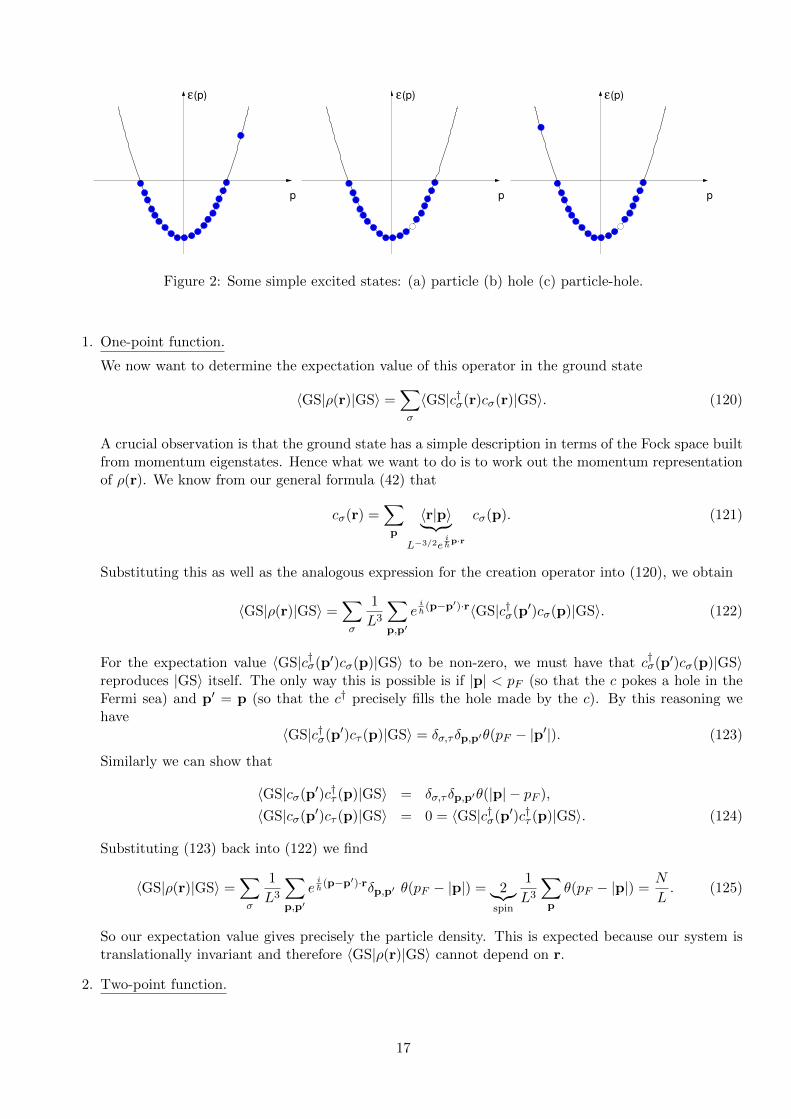
2.1.2 Excitations

• Particle excitationsc†σ(k)|GS〉 with |k| > pF . (112)

Their energies and momenta are

E = EGS + ε(k) > EGS , P = k. (113)

• Hole excitationscσ(k)|GS〉 with |k| < pF . (114)

Their energies and momenta are

E = EGS − ε(k) > EGS , P = −k. (115)

• Particle-hole excitationsc†σ(k)cτ (p)|GS〉 with |k| > pF > |p|. (116)

Their energies and momenta are

E = EGS + ε(k)− ε(p) > EGS , P = k− p. (117)

2.1.3 Density Correlations

Consider the single-particle operatoro = |r〉〈r| (118)

It represents the particle density at position |r〉 as can be seen by acting on position eigenstates. In secondquantization it is

ρ(r) =∑σ

∫d3r′d3r′′ 〈r′|o|r′′〉 c†σ(r′)cσ(r′′) =

∑σ

c†σ(r)cσ(r). (119)

16

(p)

p

ε (p)

p

ε (p)

p

ε

Figure 2: Some simple excited states: (a) particle (b) hole (c) particle-hole.

1. One-point function.

We now want to determine the expectation value of this operator in the ground state

〈GS|ρ(r)|GS〉 =∑σ

〈GS|c†σ(r)cσ(r)|GS〉. (120)

A crucial observation is that the ground state has a simple description in terms of the Fock space builtfrom momentum eigenstates. Hence what we want to do is to work out the momentum representationof ρ(r). We know from our general formula (42) that

cσ(r) =∑p

〈r|p〉︸ ︷︷ ︸L−3/2e

i~p·r

cσ(p). (121)

Substituting this as well as the analogous expression for the creation operator into (120), we obtain

〈GS|ρ(r)|GS〉 =∑σ

1

L3

∑p,p′

ei~ (p−p′)·r〈GS|c†σ(p′)cσ(p)|GS〉. (122)

For the expectation value 〈GS|c†σ(p′)cσ(p)|GS〉 to be non-zero, we must have that c†σ(p′)cσ(p)|GS〉reproduces |GS〉 itself. The only way this is possible is if |p| < pF (so that the c pokes a hole in theFermi sea) and p′ = p (so that the c† precisely fills the hole made by the c). By this reasoning wehave

〈GS|c†σ(p′)cτ (p)|GS〉 = δσ,τδp,p′θ(pF − |p′|). (123)

Similarly we can show that

〈GS|cσ(p′)c†τ (p)|GS〉 = δσ,τδp,p′θ(|p| − pF ),

〈GS|cσ(p′)cτ (p)|GS〉 = 0 = 〈GS|c†σ(p′)c†τ (p)|GS〉. (124)

Substituting (123) back into (122) we find

〈GS|ρ(r)|GS〉 =∑σ

1

L3

∑p,p′

ei~ (p−p′)·rδp,p′ θ(pF − |p|) = 2︸︷︷︸

spin

1

L3

∑p

θ(pF − |p|) =N

L. (125)

So our expectation value gives precisely the particle density. This is expected because our system istranslationally invariant and therefore 〈GS|ρ(r)|GS〉 cannot depend on r.

2. Two-point function.

17

Next we want to determine the two-point function

〈GS|ρ(r)ρ(r′)|GS〉 =∑σ,τ

1

L6

∑p,p′

∑k,k′

ei~ (p−p′)·re

i~ (k−k′)·r′〈GS|c†σ(p′)cσ(p)c†τ (k′)cτ (k)|GS〉. (126)

The difficulty in calculating the ground state expectation value is that the cσ(p) (c†σ(p)) annihilatethe ground state only for |p| > pF (|p| < pF ). A way around this is to define new annihilation andcreation operators by

dσ(p) = θ(|p| − pF )cσ(p) + θ(pF − |p|)c†σ(p) , d†σ(p) =(dσ(p)

)†. (127)

These fulfil canonical anticommutation relations

{dσ(p), d†τ (k)} = δσ,τδk,p , {dσ(p), dτ (k)} = 0 , (128)

and by construction we have〈GS|c†σ(p) = 0 = cσ(p)|GS〉. (129)

This is an example of a so-called particle-hole transformation. We may now use the inverse transfor-mation

cσ(p) = θ(|p| − pF )dσ(p) + θ(pF − |p|)d†σ(p) (130)

to replace the creation and annihilation operators in (126) by the dσ(p), d†σ(p). After that we simplyapply the anticommutation relations (128) to move all annihilation operators to the right, and finallyuse (129). The result is

〈GS|c†σ(p′)cσ(p)c†τ (k′)cτ (k)|GS〉 = δk,k′δp,p′θ(pF − |p|)θ(pF − |k|)+δσ,τδp,k′δk,p′θ(|k′| − pF )θ(pF − |k|). (131)

Observe that by virtue of (123) and (124) this can be rewritten in the form

〈GS|c†σ(p′)cσ(p)|GS〉〈GS|c†τ (k′)cτ (k)|GS〉+ 〈GS|c†σ(p′)cτ (k)|GS〉〈GS|cσ(p)c†τ (k′)|GS〉 . (132)

The fact that the 4-point function (131) can be written as a sum over products of two-point functionsis a reflection of Wick’s theorem for noninteracting spin-1/2 fermions. This is not part of the syllabusand we won’t dwell on it, but apart from extra minus signs, this says that 2n-point functions aregiven by the sum over all possible “pairings”, giving rise to a product of two-point functions. In ourparticular case this gives

〈c†σ(p′)cσ(p)c†τ (k′)cτ (k)〉 = 〈c†σ(p′)cσ(p)〉〈c†τ (k′)cτ (k)〉 − 〈c†σ(p′)c†τ (k′)〉〈cσ(p)cτ (k)〉+ 〈c†σ(p′)cτ (k)〉〈cσ(p)c†τ (k′)〉, (133)

and using that the two point function of two creation or two annihilation operators is zero we obtain(132). Substituting (131) back in to (126) gives

〈GS|ρ(r)ρ(r′)|GS〉 =∑σ,σ′

1

L6

∑k,p

θ(pF − |k|)θ(pF − |p|)

+∑σ

1

L6

∑k,k′

θ(|k| − pF )θ(pF − |k′|)ei~ (k−k′)·(r−r′)

= (〈GS|ρ(r)|GS〉)2 +2

L3

∑|k|>pF

ei~k·(r−r

′) 1

L3

∑|k′|<pF

e−i~k′·(r−r′). (134)

In the limit L→∞ we can simplify this expression further.

18

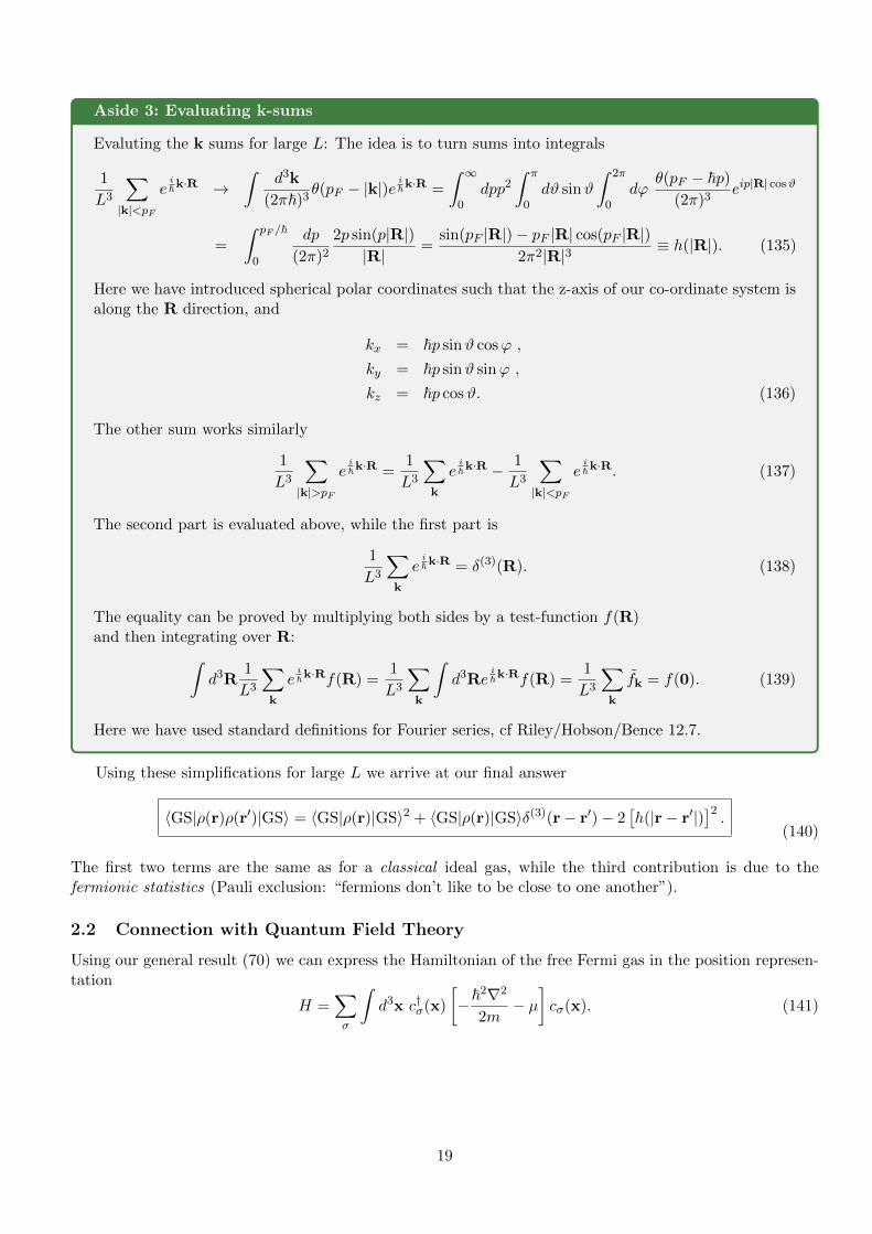
Aside 3: Evaluating k-sums

Evaluting the k sums for large L: The idea is to turn sums into integrals

1

L3

∑|k|<pF

ei~k·R →

∫d3k

(2π~)3θ(pF − |k|)e

i~k·R =

∫ ∞0

dpp2

∫ π

0dϑ sinϑ

∫ 2π

0dϕ

θ(pF − ~p)(2π)3

eip|R| cosϑ

=

∫ pF /~

0

dp

(2π)2

2p sin(p|R|)|R|

=sin(pF |R|)− pF |R| cos(pF |R|)

2π2|R|3≡ h(|R|). (135)

Here we have introduced spherical polar coordinates such that the z-axis of our co-ordinate system isalong the R direction, and

kx = ~p sinϑ cosϕ ,

ky = ~p sinϑ sinϕ ,

kz = ~p cosϑ. (136)

The other sum works similarly

1

L3

∑|k|>pF

ei~k·R =

1

L3

∑k

ei~k·R − 1

L3

∑|k|<pF

ei~k·R. (137)

The second part is evaluated above, while the first part is

1

L3

∑k

ei~k·R = δ(3)(R). (138)

The equality can be proved by multiplying both sides by a test-function f(R)and then integrating over R:∫

d3R1

L3

∑k

ei~k·Rf(R) =

1

L3

∑k

∫d3Re

i~k·Rf(R) =

1

L3

∑k

fk = f(0). (139)

Here we have used standard definitions for Fourier series, cf Riley/Hobson/Bence 12.7.

Using these simplifications for large L we arrive at our final answer

〈GS|ρ(r)ρ(r′)|GS〉 = 〈GS|ρ(r)|GS〉2 + 〈GS|ρ(r)|GS〉δ(3)(r− r′)− 2[h(|r− r′|)

]2.

(140)

The first two terms are the same as for a classical ideal gas, while the third contribution is due to thefermionic statistics (Pauli exclusion: “fermions don’t like to be close to one another”).

2.2 Connection with Quantum Field Theory

Using our general result (70) we can express the Hamiltonian of the free Fermi gas in the position represen-tation

H =∑σ

∫d3x c†σ(x)

[−~2∇2

2m− µ

]cσ(x). (141)

19

Aside 4: Schrodinger vs Heisenberg pictures and Heisenberg equation of motion

Let us consider time evolution in a system with time-independent Hamiltonian. In the Schrodingerpicture one takes the states to be time-dependent and operators to be time-independent. Timeevolution is governed by the time dependent Schrodinger equation

i~d|ψ(t)〉dt

= H|ψ(t)〉 . (142)

This is formally solved by

|ψ(t)〉 = e−i~Ht|ψ(0)〉 . (143)

Measurable quantities are related to matrix elements of observables O

〈φ(t)|O|ψ(t)〉 = 〈φ(0)| ei~HtOe−

i~Ht︸ ︷︷ ︸

O(t)

|ψ(0)〉 (144)

We see that we can calculate these in an alternative way: we can fix a basis of states at t = 0and calculate all matrix elements in this basis, while time evolution is now moved to the operators.This formulation of Quantum mechanics is known as Heisenberg picture. For a time-independentHamiltonian the time evolution of operators is then governed by the Heisenberg equation of motion

dOdt

=i

~[H,O(t)] . (145)

The Heisenberg equations of motion for cσ(x, t) are

∂cσ(x, t)

∂t= − i

~

[−~2∇2

2m− µ

]cσ(x, t). (146)

These correspond to the Euler-Lagrange equations

∂tδL

δ∂tc†σ(x, t)

= −∑a

∂aδL

δ∂ac†σ(x, t)

+δL

δc†σ(x, t)(147)

obtained from the following Lagrangian

L =∑σ

∫d3x c†σ(x, t)

[i~∂

∂t+

~2∇2

2m+ µ

]cσ(x, t) , (148)

which describes a non-relativistic Quantum Field Theory for the fermionic fields cσ(x).

2.3 “Emergent” relativistic description at low energies

Let us now for simplicity consider the case D = 1. We have seen above that the low-energy degrees offreedom “live” in the vicinities of the Fermi momenta ±pF . The expansion of cσ(x) in terms of momentummodes reads

cσ(x) =1√L

∑p

cσ(p) ei~px . (149)

Let us now imagine that we probe our Fermi system only in ways that involve very small energy transfersto the system. This kind of situation is in fact often encountered when doing experiments on solids. Suchexperimental probes are sensitive only to states that have an energy close to that of the ground state. Letus thus “project” our theory to low-energy degrees of freedom only: this amounts to retain only momentummodes in small intervals around the Fermi points

|p± pF | < Λ� pF . (150)

20

−p p

ε(p)

pFF

Figure 3: The low-energy degrees of freedom (particle/hole excitations with small excitation energies) involveonly momenta close to the Fermi points ±pF .

Here Λ is a momentum cutoff. This gives

cσ(x) −→ ei~pF x

1√L

∑|p|<Λ

cσ(pF + p) ei~px

︸ ︷︷ ︸Rσ(x)

+ e−i~pF x

1√L

∑|p|<Λ

cσ(−pF + p) ei~px

︸ ︷︷ ︸Lσ(x)

. (151)

The low-energy projection of our Hamiltonian is

H − µN −→ Hlow =∑|p|<Λ,σ

ε(pF + p)c†σ(pF + p)cσ(pF + p) + ε(−pF + p)c†σ(−pF + p)cσ(−pF + p) , (152)

where

ε(±pF + p) =(±pF + p)2

2m− µ = ±ppF

m

(1± p

2pF

)≈ ±ppF

m≡ ±vF p. (153)

Here vF is called Fermi velocity. Neglecting the small correction terms to the linear dispersion we have

Hlow ≈∑|p|<Λ,σ

vF p[c†σ(pF + p)cσ(pF + p)− c†σ(−pF + p)cσ(−pF + p)

]=

∑σ

−i~vF∫dx[R†σ(x)∂xRσ(x)− L†σ(x)∂xLσ(x)

]. (154)

This Hamiltonian is closely related to the 1+1 dimensional Dirac equation. The Lagrangian density of theDirac field is

LD = i~Ψ[γ0∂t − cγ1∂1

]Ψ−mc2ΨΨ , (155)

Here c is the speed of light, γ0 = σx and γ1 = −iσy are gamma matrices in two dimensions, Ψ = Ψ†γ0 andΨ itself is a two dimensional spinor

Ψ(x) =

(R(x)L(x)

). (156)

Writing (155) out in components we have

LD = i~[R†∂tR+ L†∂tL

]+ ic

[R†∂xR− L†∂xL

]−mc2

[R†L+ L†R

]. (157)

The corresponding Hamiltonian density

HD = −i~c[R†∂xR− L†∂xL

]+mc2

[R†L+ L†R

]. (158)

21

Comparing (154) to (158) we conclude that at low energies the Fermi gas is described by two copies (one foreach spin projection) of a massless Dirac field. The resulting theory is relativistic apart from the speed oflight being replaced by the Fermi velocity vF . This symmetry was not present in our original problem, butemerged in the vicinity of a non-trivial ground state. Such emergent descriptions of the low energy degreesof freedom in terms of relativistic QFTs are fairly common in condensed matter physics. Usually the QFTsare however strongly interacting!

2.4 Homework Questions 5-6

Question 5. Consider a system of fermions moving freely on a one-dimensional ring of length L, i.e. periodicboundary conditions are applied between x = 0 and x = L. The fermions are all in the same spin state, so thatspin quantum numbers may be omitted. Fermion creation and annihilation operators at the point x are denotedby ψ†(x) and ψ(x).a) Write down the complete set of anticommutation relation satisfied by ψ†(x1) and ψ(x2).b) Write down the wave-functions of single-particle momentum eigenstates (make sure to take the boundaryconditions into account!). What are the allowed values of momentum? Using this result, derive an expression for

the momentum space creation and annihilation operators Ψ†p and Ψp in terms of ψ†(x) and ψ(x) (hint: use thegeneral result for basis transformation obtained in the lecture notes).

c) Starting with your expression for the anticommutator {ψ†(x1), ψ(x2)}, evaluate {Ψ†p,Ψq}.d) Derive an expression for ψ(x) in terms of Ψk.e) The density operator ρ(x) is defined by ρ(x) = ψ†(x)ψ(x). The number operator is

N =

∫ L

0dx ρ(x) .

Express ρ(x) in terms of Ψ†p and Ψq, and show from this that

N =∑k

Ψ†kΨk .

Let |0〉 be the vacuum state (containing no particles) and define |φ〉 by

|φ〉 = A∏k

(uk + vkΨ†k)|0〉,

where uk and vk are complex numbers depending on the label k, and A is a normalisation constant.Evaluate (i) |A|2, (ii) 〈φ|N |φ〉, and (iii) 〈φ|N2|φ〉. Under what conditions is |φ〉 an eigenstate of particle

number?

Question 6. Consider a system of fermions in which the functions ϕ`(x), ` = 1, 2 . . . N , form a completeorthonormal basis for single particle wavefunctions.a) Explain how Slater determinants may be used to construct a complete orthonormal basis for n-particle stateswith n = 2, 3 . . . N . Calculate the normalisation constant for such a Slater determinant at a general value of n.How many independent n-particle states are there for each n?b) Let C†` and C` be fermion creation and destruction operators which satisfy the usual anticommutation relations.The quantities ak are defined by

ak =

N∑`=1

Uk`C`,

where Uk` are elements of an N × N matrix, U . Write down an expression for a†k. Find the condition which

must be satisfied by the matrix U in order that the operators a†k and ak also satisfy fermion anticommutationrelations.

22

c) Non-interacting spinless fermions move in one dimension in an infinite square-well potential, with positioncoordinate 0 ≤ x ≤ L. The normalised single particle energy eigenstates are

ϕ`(x) =

(2

L

)1/2

sin

(`πx

L

),

and the corresponding fermion creation operator is C†` .Write down expressions for C†(x), the fermion creation operator at the point x, and for ρ(x), the particle

density operator, in terms of C†` , C` and ϕ`(x).d) What is the ground state expectation value 〈ρ(x)〉 in a system of n fermions?

In the limit n→∞, L→∞, taken at fixed average density ρ0 = n/L, show that

〈ρ(x)〉 = ρ0

[1− sin 2πρ0x

2πρ0x

].

Sketch this function and comment briefly on its behaviour for x→ 0 and x→∞.

3 Linear Response Theory

Now is a good time to address the question what quantities are of experimental interest. To that end, letus consider a quantum system described by a time-independent Hamiltonian H0 that initially is in thermalequilibrium at a temperature T . Expectation values of physical observables are then given by

〈O〉β ≡1

ZTr[e−βH0O

], (159)

where β = 1/(kBT ) and Z is the partition function

Z = Tr[e−βH0

]. (160)

In terms of energy eigenstates H0|n〉 = En|n〉 we have

〈O〉β =1

Z

∑n

e−βEn〈n|O|n〉. (161)

Suppose now that we apply a very weak time-dependent external perturbation V (t) to our system thatdrives it out of thermal equilibrium. The time evolution of the system is then governed by the Hamiltonian

H(t) = H0 + V (t) . (162)

The time evolution of states is given by the time-dependent Schrodinger equation

i~∂

∂t|ψ(t)〉 = H(t)|ψ(t)〉 . (163)

As the perturbation is very weak it is useful to separate its effects on the time evolution from those of H0.This gives rise to the so-called interaction picture. We define interaction picture operators by

Aint(t) ≡ ei~H0tAe−

i~H0t . (164)

We then split the time evolution of states into the contribution from H0 and the remainder as follows

|ψ(t)〉 = e−i~H0tU(t, t0)e

i~H0t0 |ψ(t0)〉 . (165)

23

Substituting this back into (163) and using that the state is arbitrary then gives an equation for U(t, t0)

i~∂

∂tU(t, t0) = e

i~H0tV (t)e−

i~H0t U(t, t0)

= Vint(t) U(t, t0) . (166)

The solution of this equation under the conditions that U(t0, t0) = 1 is

U(t, t0) = 1− i

~

∫ t

t0

dt′ Vint(t′)− 1

~2

∫ t

t0

dt′∫ t′

t0

dt′′ Vint(t′)Vint(t

′′) + . . .

= T exp

(−i~

∫ t

t0

dt′ Vint(t′)

), (167)

where we have defined a time ordering operation by

T A(t)B(t′) =

{A(t)B(t′) if t > t′

B(t′)A(t) if t < t′. (168)

Let us now apply this formalism to the expectation value of an observable O at time t > t0, where weimagine that our perturbation vanishes for earlier times. Then

〈O(t)〉β ≡ 1

Z

∑n

e−βEn〈n(t)|O|n(t)〉

=1

Z

∑n

e−βEn〈n|U †(t, t0) Oint(t) U(t, t0)|n〉

=1

Z

∑n

e−βEn{〈n|Oint(t)|n〉 −

i

~

∫ t

t0

dt′〈n|[Oint(t), Vint(t′)]|n〉+ . . .

}≈ 〈O〉β −

i

~

∫ t

t0

dt′〈[Oint(t), Vint(t′)]〉β . (169)

Here we have used that e−i~H0t0 |n〉 = e−

i~E0t0 |n〉. Restricting our discussion to the case V (t) = f(t)V where

f(t) is a time dependent function and taking t0 → −∞ we obtain

〈O(t)〉β − 〈O〉β ≈∫ ∞−∞

dt′ χO,V (t, t′) f(t′) , (170)

where χO,V is a retarded correlation function of the operators O and V

χO,V (t, t′) = − i~θ(t− t′) 〈[Oint(t), Vint(t

′)]〉β . (171)

It is easy to see (by writing out the average in a basis of eigenstates of H0 and using (164)) that thiscorrelation function depends only on the time difference t− t′.

Let us now look at an example of this linear response formalism. Let us take the Fermi gas as our systemand perturb it by a time-dependent potential of the form

V =

∫d3r ρ(r) φext(r, t) , (172)

where ρ(r) is the particle density operator introduced previously. Imposing such a potential is readily doneexperimentally. If we then measure the density variation induced by the external potential we find accordingto our calculation above

〈ρ(r, t)〉β − 〈ρ(r)〉β ≈∫ ∞−∞

dt′∫d3r′ φext(r, t

′) χρρ(r, t; r′, t′). (173)

24

Here χρρ is the retarded density-density correlation function

χρρ(r, t; r′, t′) = − i

~θ(t− t′) 〈[ρint(r, t), ρint(r

′, t′)]〉β . (174)

This is a particular example of a response function. These are the quantities that are measured in manykinds of experiments.

4 Application II: Weakly Interacting Bosons

As you know from Statistical Mechanics, the ideal Bose gas displays the very interesting phenomenon ofBose condensation. This has been observed in systems of trapped Rb atoms and led to the award of theNobel prize in 2001 to Ketterle, Cornell and Wiemann. The atoms in these experiments are bosonic, but theatom-atom interactions are not zero. We now want to understand the effects of interactions in the frameworkof a microscopic theory. The kinetic energy operator is expressed in terms of creation/annihilation operatorssingle-particle momentum eigenstates as

T =∑p

p2

2mc†(p)c(p). (175)

Here we have assumed that our system in enclosed in a large, periodic box of linear dimension L. Theboson-boson interaction is most easily expressed in position space

V =1

2

∫d3rd3r′ c†(r)c†(r′)V (r, r′)c(r′)c(r) (176)

A good model for the potential V (r, r′) is to take it of the form

V (r, r′) = Uδ(3)(r− r′), (177)

i.e. bosons interact only if they occupy the same point in space. Changing to the momentum spacedescription

c(r) =1

L3/2

∑p

ei~p·rc(p), (178)

we have

V =U

2L3

∑p1,p2,p3

c†(p1)c†(p2)c(p3)c(p1 + p2 − p3). (179)

4.1 Ideal Bose Gas

For U = 0 we are dealing with an ideal Bose gas and we know that the ground state is a condensate: allparticles occupy the lowest-energy single-particle state, i.e. the zero-momentum state

|GS〉0 =1√N !

(c†(p = 0)

)N|0〉. (180)

So p = 0 is special, and in particular we have

0〈GS|c†(p = 0)c(p = 0)|GS〉0 = N. (181)

25

4.2 Bogoliubov Approximation

For small U > 0 we expect the Bose-Einstein condensate to persist, i.e. we expect

〈GS|c†(p = 0)c(p = 0)|GS〉 = N0 � 1. (182)

However,[c†(0)c(0), V ] 6= 0, (183)

so that the number of p = 0 bosons is not conserved, and the ground state |GS〉 will be a superposition ofstates with different numbers of p = 0 bosons. However, for the ground state and low-lying excited stateswe will have

〈Ψ|c†(0)c(0)|Ψ〉 ' N0 , (184)

where N0, crucially, is a very large number. The Bogoliubov approximation states that, when acting on theground state or low-lying excited states, we in fact have

c†(0) '√N0 , c(0) '

√N0 ,

(185)

i.e. creation and annihilation operators are approximately diagonal. This is a much stronger statement than(184), and at first sight looks rather strange. It amounts to making an ansatz for low-energy states |ψ〉 thatfulfils

〈ψ′|c(0)|ψ〉 =√N0〈ψ′|ψ〉+ . . . (186)

where the dots denote terms that are small compared to√N0. We’ll return to what this implies for the

structure of |ψ〉 a little later. Using (185) we may expand H in inverse powers of N0

H =∑p

p2

2mc†(p)c(p)

+U

2L3N2

0 +UN0

2L3

∑k 6=0

2c†(k)c(k) + 2c†(−k)c(−k) + c†(k)c†(−k) + c(−k)c(k)

+ . . . (187)

Note that there is no term that goes as N32

0 because setting the momentum of three of the creation/annihi-lation operators in (179) to zero forces the last momentum to be zero as well. Now use that

N0 = c†(0)c(0) = N −∑p6=0

c†(p)c(p), (188)

where N is the (conserved) total number of bosons, and define

ρ =N

L3= density of particles. (189)

Then our Hamiltonian becomes

H =Uρ

2N +

∑p6=0

[p2

2m+ Uρ

]︸ ︷︷ ︸

ε(p)

c†(p)c(p) +Uρ

2

[c†(p)c†(−p) + c(−p)c(p)

]+ . . .

(190)

The Bogoliubov approximation has reduced the complicated four-boson interaction to two-boson terms. Theprice we pay is that we have to deal with the “pairing”-terms quadratic in creation/annihilation operators.

26

4.3 Bogoliubov Transformation

Consider the creation/annihilation operators defined by(b(p)b†(−p)

)=

(cosh(θp) sinh(θp)sinh(θp) cosh(θp)

)(c(p)

c†(−p).

)(191)

It is easily checked that for any choice of Bogoliubov angle θp = θ−p

[b(p), b(q)] = 0 = [b†(p), b†(q)] , [b(p), b†(q)] = δp,q. (192)

In terms of the Bogoliubov bosons the Hamiltonian becomes

H = const +1

2

∑p6=0

[(p2

2m+ Uρ

)cosh(2θp)− Uρ sinh(2θp)

] [b†(p)b(p) + b†(−p)b(−p)

]−[(

p2

2m+ Uρ

)sinh(2θp)− Uρ cosh(2θp)

] [b†(p)b†(−p) + b(−p)b(p)

]+ . . . (193)

Now we choose

tanh(2θp) =Uρ

p2

2m + Uρ, (194)

as this removes the b†b† + bb terms, and leaves us with a diagonal Hamiltonian

H = const +∑p6=0

E(p)b†(p)b(p) + . . .

(195)

where

E(p) =

√(p2

2m+ Uρ

)2

− (Uρ)2 . (196)

We note that

E(p) −→ p2

2mfor |p| → ∞, (197)

which tells us that at high momenta (and hence high energies) we recover the quadratic dispersion. In thislimit θp → 0, so that the Bogoliubov bosons reduce to the “physical” bosons we started with. On the otherhand

E(p) −→√Uρ

m|p| for |p| → 0. (198)

So here we have a linear dispersion.

4.4 Ground State and Low-lying Excitations

We note that the Hamiltonian (195) involves only creation/annihilation operators with p 6= 0. Formally, wecan define zero-momentum Bogoliubov bosons as simply being equal to the original ones

b(0) = c(0) . (199)

Let us now define the Bogoliubov vacuum state |0〉 by

b(p)|0〉 = 0 . (200)

Clearly, for p 6= 0 we have E(p) > 0, and hence no Bogoliubov quasiparticles will be present in the groundstate. On the other hand, a basic assumption we made was that

〈GS|b(0)|GS〉 '√N0. (201)

27

In order to get an idea what this implies for the structure of the ground state, let us express it in the generalform

|GS〉 =∞∑n=0

αn(b†(0)

)n|0〉 . (202)

Eqn (201) then implies that

αn+1 '√N0

n+ 1αn . (203)

Replacing this approximate relation by an equality leads to a coherent state

|GS〉 = e−N0/2e√N0b†(0)|0〉. (204)

Low-lying excited states can now be obtained by creating Bogoliubov quasipartices, e.g.

b†(q)|GS〉, (205)

is a particle-excitation with energy E(q) > 0. Note that the eigenstates of the Hamiltonian are obtained byacting with the Bogoliubov creation operators on the ground state and that the “elementary excitations” aretherefore the Bogoliubov bosons rather than the original bosons. The way to understand this is to note thatthe ground state is a rather complicated many-boson state, and excitations involve the collective motion ofall these bosons. Inspection of the Bogoliubov angle (194) shows that θp goes to zero for large momenta|p|, and concomitantly b†(p) ≈ c†(p), cf. (191). In other words, at high energies the Bogoliubov bosonsessentially reduce to the original ones, which is also reflected in the dispersion relation (197).

4.5 Ground state correlation functions

We are now in a position to work out correlation functions in the ground state such as

〈GS|c†(p)c(q)|GS〉 , p,q 6= 0. (206)

Inverting the Bogoliubov transformation (191) we have

c†(p) = cosh(θp)b†(p)− sinh(θp)b(−p) ,

c(q) = cosh(θq)b(q)− sinh(θq)b†(−q) . (207)

Using that〈GS|b†(p) = 0 = b(q)|GS〉, (208)

we find that

〈GS|c†(p)c(q)|GS〉 = sinh(θq) sinh(θq)〈GS|b(−p)b†(−q)|GS〉= sinh2(θp)δq,p (p,q 6= 0). (209)

This tells us that, in contrast to the ideal Bose gas, in the ground state of the interacting Bose gas we havea finite density of bosons with non-zero momentum

〈GS|c†(p)c(p)|GS〉 = sinh2(θp) . (210)

Another feature of the ground state is that the two-point function of two annihilation/creation operators isnon-zero

〈GS|c(p)c(q)|GS〉 = 〈GS|c†(q)c†(p)|GS〉 = − cosh(θp) sinh(θq)δp,−q. (211)

28

4.6 Spontaneous Symmetry Breaking

Eqns (211) imply that boson number is not a good quantum number in the ground state. More formally,we say that the ground state spontaneously breaks the U(1) symmetry of the Hamiltonian H = T + V . Letus explain that statement. The Hamiltonian is invariant under the symmetry operation

Uc(p)U † = eiφc(p) , φ ∈ R ,

Uc†(p)U † = e−iφc†(p) , (212)

i.e.UHU † = H. (213)

The reason for this is that all terms in H involve the same number of creation as annihilation operators,and the total particle number is therefore conserved. This is referred to as a global U(1) symmetry (asthe transformations (212) form a group called U(1)). Let us now investigate how ground state expectationvalues transform. We have

〈GS|c(p)c(q)|GS〉 = 〈GS|U †Uc(p)U †Uc(q)U †U |GS〉 = e2iφ〈GS|U †c(p)c(q)U |GS〉 . (214)

If the ground state were invariant under the symmetry, we would have U |GS〉 = |GS〉. Eqn (214) would thenimply that 〈GS|c(p)c(q)|GS〉 = 0. Reversing the argument, we see that a non-zero value of the expectationvalue (211) implies that the ground state cannot be invariant under the U(1) symmetry, and in fact “breaksit spontaneously”.

4.7 Depletion of the Condensate

We started out by asserting that for small interactions U > 0 we retain a Bose-Einstein condensate, i.e. theconsensate fraction N0/N remains large. We can now check that this assumption is self-consistent. We have

N0 = N −∑p6=0

c†(p)c(p). (215)

Thus in the ground state

N0

N= 1− 1

N

∑p6=0

〈GS|c†(p)c(p)|GS〉 = 1− 1

N

∑p6=0

sinh2(θp), (216)

where we have used (209). This equals

N0

N= 1− 1

2N

∑p6=0

1√1− tanh2(2θp)

− 1

= 1− 1

2N

∑p6=0

1√1−

[Uρε(p)

]2− 1

. (217)

We again turn this into an integral and evaluate it in spherical polar coordinates, which gives

N0

N≈ 1− 2π

ρ

∫ ∞0

dp

(2π~)3p2

1√1−

[Uρε(p)

]2− 1

. (218)

By means of the substitution p =√

2mUρz we can see that the integral is proportional to U3/2 and thusindeed small for small U .

29

5 Application III: Spinwaves in a Ferromagnet

Consider the following model of a magnetic insulator: at each site r of a D-dimensional with N sites latticewe have a magnetic moment. In QM such magnetic moments are described by three spin-operators

Sαr , α = x, y, z , (219)

which fulfil the angular momentum commutation relations

[Sαr , Sβr′ ] = δr,r′iεαβγS

γr . (220)

We will assume that the spin are large in the sense that

S2r =

∑α

(Sαr)2

= s(s+ 1)� 1. (221)

Let us begin by constructing a basis of quantum mechanical states. At each site we have 2s+ 1 eigenstatesof Szr

Szr |m〉r = m|m〉r, m = s, s− 1, . . . ,−s. (222)

They can be constructed from |s〉r using spin lowering operators S−r = Sxr − iSyr

|s− n〉r =1

Nn(S−r )n|s〉r , n = 0, 1, . . . , 2s, (223)

where Nn are normalization constants. A basis of states is then given by∏r

|sr〉r , −s ≤ sr ≤ s spin on site r. (224)

5.1 Heisenberg model and spin-rotational SU(2) symmetry

An appropriate Hamiltonian for a ferromagnetic insulator was derived by Heisenberg

H = −J∑〈r,r′〉

Sr · Sr′ .

(225)

Here 〈r, r′〉 denote nearest-neighbour pairs of spins and we will assume that J > 0. The model (225) isknown as the ferromagnetic Heisenberg model. You can check that the Hamiltonian (225) commutes withthe three total spin operators

[H,Sα] = 0 , Sα =∑r

Sαr . (226)

These imply that the Hamiltonian is invariant under general rotations (in spin space)

eiα·SHe−iα·S = H. (227)

The transformations (227) form a group known as SU(2), and the Heisenberg Hamiltonian (225) is invariantunder them.

30

5.2 Exact ground states

One ground state of H is given by

|GS〉 =∏r

|s〉r.

(228)

Its energy is

H|GS〉 = −J∑〈r,r′〉

s2|GS〉 = −Js2NB|GS〉, (229)

where NB is the total number of bonds in our lattice. The total spin lowering operator S− =∑

r S−r

commutes with H by virtue of (226) and hence

|GS, n〉 =1

Nn

(S−)n |GS〉 , 0 ≤ n ≤ 2sN (230)

are ground states as well (as they have the same energy). Here Nn is a normalization.

Aside 5: Proof that |GS〉 is a ground state

We note that the spin-spin interaction can be written in the form

2Sr · Sr′ = (Sr + Sr′)2 − S2

r − S2r′ = J2 − 2s(s+ 1). (231)

Here J2 is the total angular momentum squared. Its eigenvalues follow from the theoryof adding angular momenta to be

J2|j,m〉 = j(j + 1)|j,m〉 , j = 2s, 2s− 1, . . . , 1, 0. (232)

This tells us that the maximal eigenvalue of J2 is 2s(2s+ 1), and by expanding |ψ〉 in abasis of eigenstates of J2 we can easily show that

〈ψ|J2|ψ〉 =∑

j,m,j′,m′

〈ψ|j,m〉〈j,m|J2|j′,m′〉〈j′,m′|ψ〉

=∑j,m

|〈ψ|j,m〉|2j(j + 1) ≤ 2s(2s+ 1)∑j,m

|〈ψ|j,m〉|2 = 2s(2s+ 1). (233)

This tells us that〈ψ|Sr · Sr′ |ψ〉 ≤ s2. (234)

This provides us with a bound on the eigenvalues of the Hamiltonian, as

〈ψ|H|ψ|〉 ≥ −J∑〈r,r′〉

s2 = −Js2Nz. (235)

The state we have constructed saturates this bound, so must be a ground state.

Let us now see how the SU(2) symmetry is reflected in expectation values of operators O. At finitetemperature we have

〈O〉β =1

Z(β)Tr[e−βHO

], (236)

where Z(β) = Tr[e−βH ] is the partition function and β = 1/kBT . In the T → 0 limit we have

〈O〉∞ =1

2sN + 1

2sN∑n=0

〈GS, n|O|GS, n〉, (237)

31

i.e. we average over all ground states. The thermal average, as well as its T = 0 limit, are invariant underrotations in spin space. Indeed, under a rotation in spin space we have

〈eiα·SOe−iα·S〉β =1

Z(β)Tr[e−βHeiα·SOe−iα·S

](238)

where S =∑

r Sr are the global spin operators. Using the cyclicity of the trace and the fact that Hcommutes with the global spin operators, we see that this equals 〈O〉β. If we choose as our operator O anyof the global spin operators, and consider a rotation by π around one of the orthogonal axes, we see thatthe magnetization always vanishes

〈Sα〉β = 0 , α = x, y, z. (239)

Physically this is what one would expect for a system that is spin rotationally invariant, i.e. looks the samein any direction in spin space.

5.3 Spontaneous Symmetry Breaking

In a real system, the 2sN + 1-fold ground state degeneracy is usually broken through imperfections. Inpractice the details of these imperfections are not important, the only thing that matters is that the symmetrygets broken. To keep things simple, one retains the spin-rotationally symmetric Hamiltonian, and says thatthe ground state breaks the symmetry “spontaneously”.

A convenient mathematical description of this effect is as follows. Imagine adding an infinitesimalmagnetic field −ε

∑r S

zr to the Hamiltonian. This will break the symmetry and hence the degeneracy of the

ground states, which now will have energies

EGS,n = −Js2NB − ε(sN − n). (240)

Now consider the sequence of limits

limε→0

limN→∞

[EGS,n − EGS,0] =

{0 if limN→∞

nN = 0 ,

∞ else.(241)

This means that if we define the thermodynamic limit in the above way, then the only surviving groundstates will have magnetization per site s, i.e. contain only a non-extensive number of spin flips. In all ofthese remaining ground states the spin rotational symmetry has been broken. As we have taken ε → 0our Hamiltonian is again SU(2) symmetric, but the remaining ground states “spontaneously” break thissymmetry.

5.4 Holstein-Primakoff Transformation

We succeeded in finding the ground states of H because of their simple structure. For more general spinHamiltonians, or even the Hamiltonian (225) with negative value of J , this will no longer work and we needa more general, but approximate way of dealing with such problems. This is provided by (linear) spinwavetheory.

As shown by Holstein and Primakoff, spin operators can be represented in terms of bosonic creation andannihilation operators as follows:

Szr = s− a†rar , S+r = Sxr + iSyr =

√2s

√1− a†rar

2sar . (242)

You can check that the bosonic commutation relations

[ar, a†r′ ] = δr,r′ (243)

32

imply that[Sαr , S

βr′ ] = δr,r′iεαβγS

γr . (244)

However, there is a caveat: the spaces of QM states are different! At site r we have(Sr)n|s〉r , n = 0, . . . , 2s (245)

for spins, but for bosons there are infinitely many states(a†r)n|0〉r , n = 0, . . . ,∞. (246)

To make things match, we must impose a constraint, that there are at most 2s bosons per site. Now we takeadvantage of the fact that we have assumed s to be large: in the ground state there are no bosons present,because

〈GS|s− a†rar|GS〉 = 〈GS|Szr |GS〉 = s = (247)

Low-lying excited states will only have a few bosons, so for large enough s we don’t have to worry aboutthe constraint. Using the Holstein-Primakoff transformation, we can rewrite H in a 1/s expansion

H = −J∑〈r,r′〉

s2 − s[a†rar + a†r′ar′ − a

†rar′ − a

†r′ar

]+ . . .

(248)

Here the dots indicate terms proportional to s0, s−1, etc. Once again using that s is large, we drop theseterms (for the time being). We then can diagonalize H by going to momentum space

ar =1√N

∑k

eik·ra(k) , [a(k), a†(p)] = δk,p , (249)

Exercise 2: Quantization conditions for lattice “momenta”

As we are dealing with a lattice model translational invariance is now reduced to translations bymultiples of the lattice spacing in the various crystallographic directions. On a hypercubic latticewith periodic boundary conditions we have

a(r + Lea) = a(r), (250)

where ea denotes the unit vector in the a direction and L is the linear size of our system (so N = LD).In D=1 periodic boundary conditions imply that our spin model lives on a ring, and (250) then simplymeans that if we go around the ring once we return precisely to where we started. Out goal is todefine a set of N linearly independent operators

a(k) =1√N

∑r

e−ik·rar . (251)

Using (250) we conclude that

a(k) =1√N

∑r

e−ik·rar+Lea =1√N

∑r

e−ik·(r−Lea)ar, (252)

33

which leads to the conditionseiLk·ea = 1. (253)

A solution to these conditions that provides us with linearly independent a(k)’s is

ka =2π

Lna , na = 1, 2, . . . , L. (254)

Let us now work out the commutation relations

[a(k), a†(p)] =1

N

∑r,r′

e−ik·reip·r′[a(r), a†(r′)]︸ ︷︷ ︸

δr,r′

=1

N

∑r

e−i(k−p)·r =1

N

D∏a=1

L∑ra=1

e−i(ka−pa)ra

︸ ︷︷ ︸Lδka,pa

= δk,p. (255)

In terms of creation and annihilation operators in momentum space the Hamiltonian becomes

H = −Js2Nz +∑q

ε(q)a†(q)a(q) + . . .

(256)

For a simple cubic lattice the energy is

ε(q) = 2Js [3− cos qx − cos qx − cos qz] . (257)

For small wave numbers this is quadratic

ε(q) ≈ Js|q|2 for |q| → 0. (258)

In the context of spontaneous symmetry breaking these gapless excitations are known as Goldstone modes.Let us now revisit the logic underlying our 1/s expansion. For things to be consistent, we require that

the terms of order s in (256) provide only a small correction to the leading contribution proportional to s2.This will be the case as long as we are interested only is states |Ψ〉 such that

〈Ψ|a†(q)a(q)|Ψ〉 � s. (259)

This condition is certainly fulfilled for the ground state and low-lying excited states.

5.4.1 Heisenberg Antiferromagnet

Another example to which spinwave theory can be fruitfully applied is the model

H = J∑〈r,r′〉

Sr · Sr′ , (260)

where 〈r, r′〉 denote nearest-neighbour pairs of spins on a simple cubic lattice and J > 0. Compared to (225)all we have done is to switch the overall sign of H, but this has important consequences. In particular, it isno longer possible to obtain an exact ground state for the model. Instead, we start by considering our spinsto be classical. This is justified if we are interested only in states with large spin quantum numbers. Wewill assume this to be the case and check the self-consistency of our assumption later. In the classical limitwe can think of the spins as three-dimensional vectors. The lowest energy configuration is then one, whereall neighbouring spins point in opposite directions, i.e. along the three cystal axes the spin configuration

34

looks like ↑↓↑↓↑↓ .... This is known as a Neel state. It is convenient to subdivide our lattice into twosublattices: on sublattice A all spins point in the same direction, while on sublattice B all spins point inthe opposite direction. Like the ferromagnet, the model (260) has a global spin-rotational symmetry, thatwill be spontaneously broken in the ground state. By choosing our spin quantization axis appropriately, theclassical ground state can then be written in the form∏

r∈A|s〉r

∏r′∈B| − s〉r′ (261)

The idea is now to map this state to a ferromagnetic one, by inverting the spin quantization axis in the Bsublattice. After that we can employ the Holstein-Primakoff transformation to carry out a 1/s expansion.As a result of the rotation of spin quatization axis on the B sublattice, the part of the Hamiltonian of orders now contains terms involving two annihilation or two creation operators. Diagonalizing the Hamiltonianthen requires a Bogoliubov transformation.

5.5 Homework Questions 7-8

Question 7. A magnetic system consists of two types of Heisenberg spin SA and SB located respectively onthe two inter-penetrating sublattices of an NaCl crystal structure (i.e. a simple cubic structure with alternate Aand B in any Cartesian direction). Its Hamiltonian is

H = J∑i,j

SAi · SBj

where the i, j are nearest neighbours, respectively on the A and B sublattices. J is positive. Show that theclassical ground state has all the A spins ferromagnetically aligned in one direction and all the B spins ferromag-netically aligned in the opposite direction. Assume the quantum mechanical ground state is well approximatedby the classical one. To a first approximation the spin operators are given in terms of boson operators a, b by

A sublattice B sublatticeSzi = SA − a†iai Szj = −SB + b†jbjS+i ≡ Sxi + iSyi ' (2SA)1/2ai S+

j ≡ Sxj + iSyj ' (2SB)1/2b†jS−i ≡ Sxi − iSyi ' (2SA)1/2a†i S−j ≡ Sxj − iSyj ' (2SB)1/2bj

Discuss the validity of this approximation. Use these relations to express the Hamiltonian in terms of the bosonoperators to quadratic order.

Transforming to crystal momentum space using (with N the number of sites on one sublattice)

ai = N−1/2∑k

e−ik·riak, bj = N−1/2∑k

eik·rjbk

show that your result can be expressed in the form

H = E0 +∑k

[Aka

†kak +Bkb

†kbk + Ck(a†kb

†k + bkak)

]and determine the coefficients. Hence calculate the spectrum of excitations at low momenta. Consider both thecases with SA = SB and SA 6= SB and comment on your results.

Question 8. (optional) Consider the ideal Fermi gas at finite density N/V in a periodic 3-dimensional boxof length L.(a) Give an expression of the ground state in terms of creation operators for momentum eigenstates.(b) Calculate the single-particle Green’s function

Gστ (ω,q) =

∫dt eiω(t−t′)

∫d3r e−iq·(r−r

′)Gστ (t, r; t′, r′) ,

Gστ (t, r; t′, r′) = −i〈GS|Tcσ(r, t) c†τ (r′, t′)|GS〉, (262)

35

where T denotes time-ordering (i.e. TO(t1)O(t2) = θ(t1 − t2)O(t1)O(t2)− θ(t2 − t1)O(t2)O(t1) for fermionicoperators), and

cσ(r, t) ≡ ei~Htcσ(r)e−

i~Ht. (263)

First express the creation/annihilation operators c†σ(r, t), cσ(r, t) in terms of creation/annihilation operators in

momentum space c†σ(p, t), cσ(p, t). Then show that for annihilation operators in momentum space we have

cσ(p, t) ≡ ei~Htcσ(p)e−

i~Ht = cσ(p)e−

i~ tε(p) , (264)

where ε(p) = p2/2m− µ. Use this to show that

cσ(r, t) =1

L3/2

∑p

e−i~ tε(p)+ip·r cσ(p). (265)

Now insert (265) into (262) and evaluate the ground state expectation value to obtain an integral representationfor Gστ (t, r; t′, r′). Why does the Green’s function only depend on t− t′ and r−r′? Finally, calculate Gστ (ω,q).

Note: the imaginary part of the single-particle Green’s function is (approximately) measured by angle resolvedphotoemission (ARPES) experiments.

36

Part II

Phases and Phase Transitions

Physically a phase transition is a point in parameter space, where the physical properties of a many-particlesystem undergo a sudden change. An example is the paramagnet to ferromagnet transition in Fe or Ni, acartoon of which is shown in Fig. 4.

Figure 4: Equilibrium phase diagram for the paramagnetic to ferromagnetic transition. The magnetizationM(h, T ) jumps when crossing zero for T < Tc. When lowering the temperature at h = 0+ a spontaneousmagnetization develops at a critical temperature T = Tc and grows with decreasing temperature.

Mathematically a phase transition is a point in parameter space, where the free energy F = −kBT ln(Z)becomes a nonanalytic function of one of its parameters (i.e. F or some of its derivatives becomes singularor discontinuous) in the thermodynamic limit.

For a finite system this can never happen, because

Z =∑

configurations C

e−E(C)/kBT (266)

is a finite sum over finite, positive terms. Hence all derivatives are finite and well defined as well.Phase transitions are usually divided into two categories:

1. First Order Phase Transitions.

Here the free energy is continuous, but a first derivative is discontinuous. At the transition there isphase coexistence. The magnetization per site is a first order derivative of the free energy with respectto the magnetic field h. Therefore the phase transition at h = 0 and T < Tc in Fig. 4 is first order.

2. Second Order Phase Transitions.

These are characterized by a divergence in one of the higher order derivatives (“susceptibilities”) ofthe free energy. The phase transition as a function of T for h = 0 in Fig. 4 is second order.

37

6 The Ising Model

The two-dimensional square-lattice Ising model is one of the simplest statistical models to show a phasetransition and as a result has played a hugely important role in the development of the theory of criticalphenomena.

Ferromagnetism is an interesting phenomenon in solids. Some metals (like Fe or Ni) are observed toacquire a finite magnetization below a certain temperature. Ferromagnetism is a fundamentally quantummechanical effect, and arises when electron spins spontaneously align along a certain direction. The Isingmodel is a very crude attempt to model this phenomenon. It is defined as follows. We have a lattice in Ddimensions with N sites. On each site j of this lattice sits a “spin” variable σj , which can take the twovalues ±1. These are referred to as “spin-up” and “spin-down” respectively. A given set {σ1, σ2, . . . , σN}specifies a configuration. The corresponding energy is taken to be of the form

E({σj}) = −J∑〈ij〉

σiσj − hN∑j=1

σj , (267)

where 〈ij〉 denote nearest-neighbour bonds on our lattice and J > 0. The first term favours alignmenton neighbouring spins, while h is like an applied magnetic field. Clearly, when h = 0 the lowest energystates are obtained by choosing all spins to be either up or down. The question of interest is whether theIsing model displays a finite temperature phase transition between a ferromagnetically ordered phase at lowtemperatures, and a paramagnetic phase at high temperatures.

6.1 Statistical mechanics of the Ising model

The partition function of the model is

Z =∑σ1=±1

∑σ2=±1

· · ·∑

σN=±1

e−βE({σj}). (268)

The magnetization per site is given by

m(h) =1

N〈N∑j=1

σj〉β =1

Nβ

∂

∂hln(Z). (269)

The magnetic susceptibility is defined as

χ(h) =∂m(h)

∂h=

1

Nβ

∂2

∂h2ln(Z). (270)

Substituting the expression (268) for the partition function and then carrying out the derivatives it can beexpressed in the form

χ(h) =β

N

N∑l,m=1

〈σlσm〉β − 〈σl〉β〈σm〉β. (271)

6.2 The One-Dimensional Ising Model

The simplest case is when our lattice is one-dimensional, and we impose periodic boundary conditions. Theenergy then reads

E =N∑j=1

[−Jσjσj+1 −

h

2(σj + σj+1)

]≡

N∑j=1

E(σj , σj+1), (272)

where we have definedσN+1 = σ1. (273)

38

The partition function can be expressed in the form

Z =∑

σ1,...,σN

N∏j=1

e−βE(σj ,σj+1). (274)

It can be evaluated exactly by means of the transfer matrix method.

6.2.1 Transfer matrix approach

The general idea is to rewrite Z as a product of matrices. The transfer matrix T is taken to be a 2 × 2matrix with elements

Tσσ′ = e−βE(σ,σ′). (275)

Its explicit form is

T =

(T++ T+−T−+ T−−

)=

(eβ(J+h) e−βJ

e−βJ eβ(J−h)

). (276)

The partition function can be expressed in terms of the transfer matrix as follows

Z =∑

σ1,...,σN

Tσ1σ2Tσ2σ3 . . . TσN−1σNTσNσ1 (277)

As desired, this has the structure of a matrix multiplication

Z = Tr(TN).

(278)

The trace arises because we have imposed periodic boundary conditions. As T is a real symmetric matrix,it can be diagonalized, i.e.

U †TU =

(λ+ 00 λ−

), (279)

where U is a unitary matrix and

λ± = eβJ cosh(βh)±√e2βJ sinh2(βh) + e−2βJ . (280)

Using the cyclicity of the trace and UU † = I, we have

Z = Tr(UU †TN

)= Tr

(U †TNU

)= Tr

([U †TU ]N

)= Tr

(λN+ 00 λN−

)= λN+ + λN− . (281)

But as λ− < λ+ we have

Z = λN+

(1 +

[λ−λ+

]N)= λN+

(1 + e−N ln(λ+/λ−)

). (282)

So for large N , which is the case we are interested in, we have with exponential accuracy

Z ' λN+ .(283)

Given the partition function, we can now easily calculate the magnetization per site

m(h) =1

Nβ

∂

∂hln(Z). (284)

In Fig. 5 we plot m(h) as a function of inverse temperature β = 1/kBT for two values of magnetic field h.We see that for non-zero h, the magnetization per site takes its maximum value m = 1 at low temperatures.At high temperatures it goes to zero. This is as expected, as at low T the spins align along the directionof the applied field. However, as we decrease the field, the temperature below which m(h) approaches unitydecreases. In the limit h→ 0, the magnetization per site vanishes at all finite temperatures. Hence there isno phase transition to a ferromagnetically ordered state in the one dimensional Ising model.

39

2 4 6 8 10

Β

0.2

0.4

0.6

0.8

1.0

mHh=0.1L

2 4 6 8 10

Β

0.2

0.4

0.6

0.8

1.0

mHh=10-5L

Figure 5: Magnetization per site as a function of inverse temperature for two values of applied magneticfield. We see that when we reduce the magnetic field, the temperature region in which the magnetization isessentially zero grows.

6.2.2 Averages of observables in the transfer matrix formalism

The average magnetization at site j is

〈σj〉β =1

Z

∑σ1,...,σN

σje−βE({σj}). (285)

We can express this in terms of the transfer matrix as

〈σj〉β =1

Z

∑σ1,...,σN

Tσ1σ2Tσ2σ3 . . . Tσj−1σjσjTσjσj+1 . . . TσNσ1 . (286)

Using that(Tσz)σj−1σj

= Tσj−1σjσj , (287)

where σz =

(1 00 −1

)is the Pauli matrix, we obtain

〈σj〉β =1

ZTr[T j−1σzTN−j+1

]=

1

ZTr[TNσz

]. (288)

Diagonalizing T by means of a unitary transformation as before, this becomes

〈σj〉β =1

ZTr[U †TNUU †σzU

]=

1

ZTr

[(λN+ 00 λN−

)U †σzU

]. (289)

The matrix U is given in terms of the normalized eigenvectors of T

T |±〉 = λ±|±〉 (290)

asU = (|+〉, |−〉). (291)

For h = 0 we have

U |h=0 =1√2

(1 11 −1

). (292)

This gives

〈σj〉β∣∣∣h=0

= 0. (293)

40

For general h the expression is more complicated

U =

α+√1+α2

+

α−√1+α2

−1√

1+α2+

1√1+α2

−

, α± =

√1 + e4βJ sinh2(βh)± e2βJ sinh(βh). (294)

The magnetization per site in the thermodynamic limit is then

limN→∞

〈σj〉β = limN→∞

(α2

+−1

α2++1

)λN+ +

(α2−−1

α2−+1

)λN−

λN+ + λN−=

(α2

+ − 1

α2+ + 1

). (295)

This now allows us to prove, that in the one dimensional Ising model there is no phase transition at anyfinite temperature:

limh→0

limN→∞

〈σj〉β = 0 , β <∞.(296)

Note the order of the limits here: we first take the infinite volume limit at finite h, and only afterwardstake h to zero. This procedure allows for spontaneous symmetry breaking to occur, but the outcome of ourcalculation is that the spin reversal symmetry remains unbroken at any finite temperature.

Similarly, we find

〈σjσj+r〉β =1

ZTr[T j−1σzT rσzTN+1−j−r] =

1

ZTr

[U †σzU

(λr+ 00 λr−

)U †σzU

(λN−r+ 0

0 λN−r−

)]. (297)

We can evaluate this for zero field h = 0

〈σjσj+r〉β∣∣∣h=0

=λN−r+ λr− + λN−r− λr+

λN+ + λN−≈[λ−λ+

]r= e−r/ξ. (298)

So in zero field the two-point function decays exponentially with correlation length

ξ =1

ln coth(βJ). (299)

6.3 The Two-Dimensional Ising Model

We now turn to the 2D Ising model on a square lattice with periodic boundary conditions. The spin variableshave now two indices corresponding to rows and columns of the square lattice respectively

σj,k = ±1 , j, k = 1, . . . , N. (300)

The boundary conditions are σk,N+1 = σk,1 and σN+1,j = σ1,j , which correspond to the lattice “living” onthe surface of a torus. The energy in zero field is

E({σk,j}) = −J∑j,k

σk,jσk,j+1 + σk,jσk+1,j . (301)

6.3.1 Transfer Matrix Method

The partition function is given by

Z =∑{σj,k}

e−βE({σk,j}). (302)

The idea of the transfer matrix method is again to write this in terms of matrix multiplications. Thedifference to the one dimensional case is that the transfer matrix will now be much larger. We start byexpressing the partition function in the form

Z =∑{σj,k}

e−β∑Nk=1 E(k;k+1), (303)

41

k,j

j

k

σ

Figure 6: Ising model on the square lattice.

where

E(k; k + 1) = −JN∑j=1

σk,jσk+1,j +1

2[σk,jσk,j+1 + σk+1,jσk+1,j+1] . (304)

This energy depends only on the configurations of spins on rows k and k + 1, i.e. on spins σk,1, . . . , σk,Nand σk+1,1, . . . , σk+1,N . Each configuration of spins on a given row specifies a sequence s1, s2, . . . , sN withsj = ±1. Let us associate a vector

|s〉 (305)

with each such sequence. By construction there 2N such vectors. We then define a scalar product on thespace spanned by these vectors by

〈t|s〉 =

N∏j=1

δtj ,sj . (306)

With this definition, the vectors {|s〉} form an orthonormal basis of a 2N dimensional linear vector space.In particular we have

I =∑s

|s〉〈s|. (307)

Finally, we define a 2N × 2N transfer matrix T by

〈σk|T |σk+1〉 = e−βE(k;k+1). (308)

The point of this construction is that the partition function can now be written in the form

Z =∑σ1

∑σ2

· · ·∑σN

〈σ1|T |σ2〉〈σ2|T |σ3〉 . . . 〈σN−1|T |σN 〉〈σN |T |σ1〉 (309)

We now may use (307) to carry out the sums over spins, which gives

Z = Tr[TN], (310)

where the trace is over our basis {|s〉|sj = ±1} of our 2N dimensional vector space. Like in the 1D case,thermodynamic properties involve only the largest eigenvalues of T . Indeed, we have

Z =

2N∑j=1

λNj , (311)

42

where λj are the eigenvalues of T . The free energy is then

F = −kBT ln(Z) = −kBT ln

λNmax

2N∑j=1

(λjλmax

)N = −kBTN ln(λmax)− kBT ln

∑j

(λjλmax

)N , (312)

where λmax is the largest eigenvalue of T , which we assume to be unique. As |λj/λmax| < 1, the secondcontribution in (312) is bounded by −kBTN ln(2), and we see that in the thermodynamic limit the freeenergy per site is

f = limN→∞

F

N2= lim

N→∞−kBT

Nln(λmax).

(313)

Thermodynamic quantities are obtained by taking derivatives of f and hence only involve the largest eigen-value of T . The main complication we have to deal with is that T is still a very large matrix. This posesthe question, why we should bother to use a transfer matrix description anyway? Calculating Z from itsbasic definition (302) involves a sum with 2N

2terms, i.e. at least 2N

2operations on a computer. Finding

the largest eigenvalue of a M ×M matrix involves O(M2) operations, which in our case amounts to O(22N ).For large values of N this amounts to an enormous simplification.

6.3.2 Spontaneous Symmetry Breaking

Surprisingly, the transfer matrix of the 2D Ising model can be diagonalized exactly. Unfortunately wedon’t have the time do go through the somewhat complicated procedure here, but the upshot is that the2D Ising model can be solved exactly. Perhaps the most important result is that in the thermodynamiclimit the square lattice Ising model has a finite temperature phase transition between a paramagnetic anda ferromagnetic phase. The magnetization per site behaves as shown in Fig.7. At low temperatures T < Tc

1 T/T

m(T)

c

1

Figure 7: Phase Transition in the square lattice Ising model.

there is a non-zero magnetization per site, even though we did not apply a magnetic field. This is surprising,because our energy (301) is unchanged if we flip all spins

σj,k → −σj,k. (314)

The operation (314) is a discrete (two-fold) symmetry of the Ising model. Because we have translationalinvariance, the magnetization per site is

m = 〈σj,k〉β. (315)

Hence a non-zero value of m signifies the spontaneous breaking of the discrete symmetry (314). In order todescribe this effect mathematically, we have to invoke a bit of trickery. Let us consider zero temperature.

43

Then there are exactly two degenerate lowest energy states: the one with all spins σj,k = +1 and the onewith all spins σj,k = −1. We now apply a very small magnetic field to the system, i.e. add a term

δE = −ε∑j,k

σj,k (316)

to the energy. This splits the two states, which now have energies

E± = −JNB ∓ εN , (317)

where NB is the number of bonds. The next step is key: we now define the thermodynamic limit of the freeenergy per site as

f(T ) ≡ limε→0

limN→∞

−kBT ln(Z)

N2. (318)

The point is that the contributions Z± = e−βE± of the two states to Z are such that

Z−Z+

= e−2εN/kBT . (319)

This goes to zero when we take N to infinity! So in the above sequence of limits, only the state with allspins up contributes to the partition function, and this provides a way of describing spontaneous symmetrybreaking! The key to this procedure is that

limε→0

limN→∞

Z 6= limN→∞

limε→0

Z.

(320)

The procedure we have outlined above, i.e. introducing a symmetry breaking field, then taking the infinitevolume limit, and finally removing the field, is very general and applies to all instances where spontaneoussymmetry breaking occurs.

6.4 Homework Questions 9-11

Question 9. A lattice model for non-ideal gas is defined as follows. The sites i of a lattice may be empty oroccupied by at most one atom, and the variable ni takes the values ni = 0 and ni = 1 in the two cases. Thereis an attractive interaction energy J between atoms that occupy neighbouring sites, and a chemical potential µ.The model Hamiltonian is

H = −J∑〈ij〉

ninj − µ∑i

ni , (321)

where∑〈ij〉 is a sum over neighbouring pairs of sites.

(a) Describe briefly how the transfer matrix method may be used to calculate the statistical-mechanical propertiesof one-dimensional lattice models with short range interactions. Illustrate your answer by explaining how thepartition function for a one-dimensional version of the lattice gas, Eq. (1), defined on a lattice of N sites withperiodic boundary conditions, may be evaluated using the matrix

T =

(1 eβµ/2

eβµ/2 eβ(J+µ)

).

(b) Derive an expression for 〈ni〉 in the limit N →∞, in terms of elements of the eigenvectors of this matrix.(c) Show that

〈ni〉 =1

1 + e−2θ,

wheresinh(θ) = exp(βJ/2) sinh(β[J + µ]/2) .

44

Sketch 〈ni〉 as a function of µ for βJ � 1, and comment on the physical significance of your result.

Question 10. The one-dimensional 3-state Potts model is defined as follows. At lattice sites i = 0, 1, . . . , L“spin” variables σi take integer values σi = 1, 2, 3. The Hamiltonian is then given by

H = −JL−1∑i=0

δσi,σi+1 , (322)

where δa,b is the Kronecker delta, J > 0.(a) What are the ground states and first excited states for this model?(b) Write down the transfer matrix for (322). Derive an expression for the free energy per site f in the limitof large L in terms of the transfer matrix eigenvalues. Show that vectors of the form (1, z, z2) with z3 = 1 areeigenvectors, and hence find the corresponding eigenvalues. Show that at temperature T (with β = 1/kBT ) andin the limit L→∞

f = −kBT ln(

3 + eβJ − 1). (323)

(c) The boundary variable σ0 is fixed in the state σ0 = 1. Derive an expression (for large L), that the variableat site `� 1 is in the same state, in terms of the transfer matrix eigenvalues and eigenvectors. Show that yourresult has the form

〈δσ`,1〉 =1

3+

2

3e−`/ξ. (324)

How does ξ behave in the low and high temperature limits?

Question 11. Consider a one dimensional Ising model on an open chain with N sites, where N is odd. On alleven sites a magnetic field 2h is applied, see Fig. 8. The energy is

E = −JN−1∑j=1

σjσj+1 + 2h

(N−1)/2∑j=1

σ2j . (325)

(a) Show that the partition function can be written in the form

2h

1 NJ J J J J J J J

2h 2h 2h

Figure 8: Open Ising chain with magnetic field applied to all even sites.

Z = 〈u|T (N−1)/2|v〉 , (326)

where T is an appropriately constructed transfer matrix, and |u〉 and |v〉 two dimensional vectors. Give explicitexpressions for T , |u〉 and |v〉.(b) Calculate Z for the case h = 0.

6.5 Peierls Argument

The 2D Ising model can be solved exactly by the transfer matrix method introduced above. Interestingly,it is possible to establish the existence of a finite-temperature phase transition in the model without solvingit. This was pioneered by Sir Rudolf Peierls, who was the Wykeham Professor of Theoretical Physics at

45

Oxford for many years and during his career made numerous ground breaking contributions in particular tocondensed matter physics.

The Peierls argument is a nice way of establishing that the 2D square lattice Ising model has magneticlong-range order at sufficiently low temperatures without actually solving the model. Given that at very hightemperature there is no magnetic order, this shows that there must be at least one phase transition at afinite temperature.

Consider the Ising model on the square lattice with boundary conditions such that all spins on theboundary are up, i.e. take the value +1. You can think of these boundary conditions as a symmetrybreaking field. The bulk magnetic field is taken to be zero. Configurations look like the one shown in Fig. 9,and can be characterized by domains walls. These are lines separating + and − spins such that

1. The + (−) spins lie always to the left (right) of the wall.

2. Where ambiguities remain, the wall is taken to bend to the right.

3. The length of the wall is defined as the number of lattice spacings it traverses.

Figure 9: A configuration of spins and the corresponding domain walls.

A wall of length b encloses at most b2/16 spins. The total number of domain walls of length b, m(b), isbounded by

m(b) ≤ 4Nt3b−1,

(327)

where Nt is the total number of sites. This can be seens as follows:

• the first link can go into less than 4Nt positions (starting at an arbitrary site and going in any of thefour possible directions).

• subsequent links have at most 3 possible directions each.

Let us denote the i’th domain wall of length b by (b, i). Next consider a particular configuration σ = {σj,k}of spins on the lattice, and define

Xσ(b, i) =

{1 if (b,i) occurs in σ

0 else(328)

Then the total number of − spins in σ is bounded by

N− ≤∑b

b2

16

m(b)∑i=1

Xσ(b, i), (329)

46

because each spin is enclosed by at least one domain wall due to our choice of boundary conditions. Takingthermal averages, we have

〈N−〉β ≤∑b

b2

16

m(b)∑i=1

〈Xσ(b, i)〉β. (330)

Here the thermal average of Xσ(b, i) can be written as

〈Xσ(b, i)〉β =1

Z

∑σ

′e−βE(σ), (331)

where the sum is only over configurations, in which (b, i) occurs. Now consider the configuration σ′ obtainedfrom σ by reversing the spins inside the domain wall (b, i). Clearly the energies of the two configurations

Figure 10: Configurations σ and σ′ related by reversing all spins inside the domain wall (b, i). Shown areall the bonds whose energies have been changed from −J to J .

are related byE(σ) = E(σ′) + 2bJ. (332)

This can be used to obtain a bound on Z

Z ≥∑σ′

′e−βE(σ′) ≥

∑σ

′e−βE(σ)e2bJβ, (333)

where the first sum is only over configurations in which (b, i) occurs, and where we then have flipped allspins inside the domain wall. This gives us a bound on

〈Xσ(b, i)〉β =1

Z

∑σ

′e−βE(σ) ≤ e−2bJβ. (334)

47

Now we put everything together

〈N−〉β ≤∑b

b2

16

m(b)∑i=1

e−2βJb ≤∑b

b2

164Nt3

b−1e−2βJb =Nt

12

∑b=4,6,8,...

b2[3e−2βJ

]b. (335)

The sum over b can now be easily carried out, and the results at small T (large β) is

〈N−〉β ≤ 108Nte−8βJ .

(336)

So, at low temperatures we have

〈N−〉βNt

� 1

2.

(337)

This proves the existence of a spontaneous magnetization at low temperatures.

6.6 Mean Field Theory

Consider the Ising model on a D-dimensional lattice with coordination number (number of nearest neighboursites) z

E = −J∑〈ij〉

σiσj − h∑j

σj . (338)

Here 〈ij〉 denotes nearest neighbour bonds, and each bond is counted once. The magnetization per site is

m =1

N

N∑j=1

〈σj〉β. (339)

We now rewrite the energy usingσi = m+ (σi −m). (340)

In particular we have

σiσj = m2 +m(σj −m) +m(σi −m) + (σi −m)(σj −m). (341)

The idea of the mean-field approximation is to assume that the deviations σj −m of the spins from theiraverage values are small, and to neglect the terms quadratic in these fluctuations. This gives

EMF = −J∑〈ij〉

−m2 +m(σi + σj)− h∑j

σj .

(342)

Physically, what we have done is to replace the interaction of a given spin with its neighbours by an averagemagnetic field. We can simplify (342) further by noting that

−J∑〈ij〉

−m2 = Jm2Nz

2,

∑〈ij〉

σi + σj = z∑j

σj . (343)

The mean-field energy then becomes

EMF =JNz

2m2 − (Jzm+ h)

N∑j=1

σj .

(344)

48

The partition function in the mean-field approximation is

ZMF =∑{σj}

e−βEMF = e−NJzβm2

2

∑σ1

· · ·∑σN

N∏j=1

eβ(Jzm+h)σj

= e−NJzβm2

2

[∑σ1

eβ(Jzm+h)σ1

]. . .

[∑σN

eβ(Jzm+h)σN

]

= e−NJzβm2

2 [2 cosh(Jzmβ + hβ)]N . (345)

The magnetization per site is

m =1

N

N∑j=1

〈σj〉β = 〈σN 〉β, (346)

where we have used translational invariance in the last step. In mean field theory we have

m = 〈σj〉β =1

ZMFe−

NJzβm2

2

∑σ1

· · ·∑σN

σN

N∏j=1

eβ(Jzm+h)σj = tanh(Jzmβ + βh).

(347)

This is a self-consistency equation for m.

6.7 Solution of the self-consistency equation for h = 0

For zero field the self-consistency equation reads

m = tanh(Jzmβ). (348)

This can be solved graphically by looking for intersections of the functions g1(m) = tanh(Jzmβ) andg2(m) = m. There are either one or three solutions

m =

{0 if Jzβ < 1

±m0, 0 if Jzβ > 1. (349)

We still have to check whether these solutions correspond to mimima of the free energy per site. The latteris

fMF = − 1

βNln(ZMF) =

Jzm2

2− 1

βln[2 cosh(Jzmβ)]. (350)

We have∂2fMF

∂m2= Jz

[1− Jzβ

cosh(Jzmβ)

]. (351)

This is negative for m = 0 and Jzβ > 1, and hence this solution corresponds to a maximum of the freeenergy and hence must be discarded. This leaves us with

m =

{0 if T > Tc

±m0 if T < Tc,

(352)

where the transition temperature is

Tc =Jz

kB. (353)

49

6.8 Vicinity of the Phase Transition

Let us define a dimensionless variable, that measures the distance in temperature to the phase transition

t =T − TcTc

. (354)

For |t| � 1 we obtain the following results

1. Magnetization per site

m∣∣∣h=0'

{0 if T > Tc,√−3t if T < Tc.

(355)

2. Magnetic susceptibility in zero field

χ =∂m

∂h

∣∣∣h=0'

{1

kBTct−1 if T > Tc,

12kBTc

(−t)−1 if T < Tc,(356)

3. Free energy per site and heat capacity per volume

fMF

∣∣∣h=0' −kBT ln 2 +

{0 if T > Tc

−3kBTc4 t2 if T < Tc.

(357)

C

V= −T ∂

2fMF

∂T 2

∣∣∣h=0'

{0 if T > Tc3kB

2 if T < Tc.(358)

7 Critical Behaviour and Universality

Close to a critical point thermodynamic functions display power-law behaviours characterized by criticalexponents. We will now discuss various such exponents, using as a specific example the paramagnet toferromagnet transition.

1. Order Parameter

This is a quantity that is different in the various phases and can be used to characterize the phasetransition. For the paramagnet to ferromagnet transition in zero magnetic field the appropriate orderparameter is the magnetization per site

m(T ) = limh→+0

limV→∞

1

VM(h, T ).

(359)

Here M(h, T ) is the magnetization. Where T ≈ Tc, one has

m(T ) ∼

{0 if T > Tc

|t|β if T < Tct =

T − TcTc

.

(360)

β is a critical exponent.

50

ferromagnet T/T

m(T)

c

1

1

paramagnet

Figure 11: Order parameter for the paramagnet to ferromagnet transition in zero field.

2. Susceptibilities

At the critical point the system is very sensitive to external perturbations. The singularity in theresponse of the order parameter to a field “conjugate” to it is characterized by critical exponents γ±.For our magnet

χ±(T ) =∂

∂h

∣∣∣h=0

limV→∞

1

VM(h, T ) ∼ |t|−γ± .

(361)

Figure 12: Critical behaviour of the magnetic susceptibility.

3. Heat Capacity

A third critical exponent is associated with the heat capacity

C(T ) = −T ∂2F

∂T 2∼

{A+|t|−α+ if T > Tc

A−|t|−α− if T < Tc.(362)

Depending on the signs of α± this may or may not be singular, see Fig. 13.

7.1 Universality

The critical exponents are insensitive to microscopic details of the system under consideration and arecharacteristic of the critical point. A consequence of this is that completely different systems can exhibit

51

Figure 13: Critical behaviour of the heat capacity.

the same critical behaviour!

8 Landau Theory

Landau Theory is a general approach to phase transitions that

• is phenomenological in nature and deals only with macroscopic quantities;

• applies only to the neighbourhood of a critical point, where the order parameter is small.

Landau theory is constructed as follows.

1. Identify the order parameter(s) M(r) characterizing the phase transition. Depending on which phasetransition we are dealing with M can be a real scalar, a complex scalar, a real or complex vectoror something more complicated. For the simplest case of a paramagnet to ferromagnet transition theorder parameter is the magnetization per site, i.e. a real number. What we mean by simplest case hereis that at a microscopic level the magnetic moments are like Ising spins, i.e. point either in a particulardirection or in the opposite direction. The situation where the magnetic moments are modelled byvectors that can point in any direction can also be treated by the method we will now describe.

2. Form a “coarse-grained” order parameter density Φ(r). Think of this as the microscopic order param-eter averaged over atomic distances. This is a continuum field. For the example of the paramagnet toferromagnet transition we are dealing with a real scalar field.

3. Consider the free energy density to be a functional of the order parameter field Φ(r). The free energyis then

βF =

∫dDrf [Φ(r)].

(363)

4. By construction of the order parameter(s), the latter is (are) small close to our critical point. Thisallows us to expand f [Φ(r)] is a power series around Φ = 0. From now on we will focus on the simplestcase of a real scalar order parameter φ(r). Then the series expansion is

f [φ] ' const− hφ+ α2φ2 +

1

2|∇φ|2 + α3φ

3 + α4φ4 + . . .

(364)

52

where the coefficient of the gradient term is fixed by convention to be 1/2 (basically this amounts to arescaling of the order parameter by a constant and using the re-scaled quantity as our order parameterfield). This makes φ in general dimensionful

dim[φ(r)] = (length)1−D/2. (365)

The only linear term that is not a total derivative is −hφ, where h is an external field (a “source”) cou-pling to the order parameter. Total derivative terms can be dropped, because the only give boundarycontributions to F . The coefficients αn are a priori all functions of temperature and magnetic field.

5. In translationally invariant systems the free energy is minimized by r-independent order parameters(i.e. ∇φ(r) = 0). The reason is that 1

2 |∇φ|2 ≥ 0, and hence this contribution to F is minimized

by constant solutions. For constant field h the potential V (φ(r)) = −hφ + α2φ2 + α3φ

3 + α4φ4 is

also minimized by constant solutions. In order to understand the nature of the phase transition, wetherefore can simply look at the minima of the potential V (φ).

6. Finally, we use symmetries and the fact that we are interested in the vicinity of a critial point toconstrain the αj .

• If we truncate our expansion at order φ4, then thermodynamic stability requires

α4 > 0.(366)

If α4 < 0 the free energy density would be unbounded from below and could become infinitelynegative, which is forbidden.

• If we know that the system is invariant under certain symmetry operations, e.g.

φ→ −φ, (367)

then the free energy must respect this symmetry. A ferromagnet has the symmetry (367) inabsence of a magnetic field because of time-reversal invariance. Hence we must have α3 = 0 inthis case.

• In the case h = α3 = 0, for a translationally invariant system, we can obtain the temperaturedependence of α2 as follows. As discussed above, the nature of the phase transition can be inferredfrom the minima of the potential V (φ) = α2φ

2 + α4φ4. This is done in Fig. 14. We see that the

phase transition corresponds to α2 changing sign at T = Tc. So in the vicinity of the transitionwe have (by Taylor expanding α2 in T − Tc)

α2(t) = At+O(t2) , t =T − TcTc

, A > 0.

(368)

The parameter α4 is also temperature dependent, but this dependence is subleading

α4(t) = α4(0) +O(t). (369)

7. If we have α3 < 0 the transition is generically first order. To see this we again use that in a trans-lationally invariant system the minima of the free energy density will be r-independent, so that wemerely need to scrutinize the potential V (φ) to understand the nature of the phase transition. InFig. 15 we plot V (φ) when α2 is decreased at fixed α3, α4. We see that initially the minimum occursat φ = 0 (no order), and at some critical value of α2 then jumps from zero to a finite value φ0. Thisis characteristic of a first order transition.

53

Figure 14: Minima of the potential V (φ). For α2 > 0 the minima occurs at φ = 0, so there is no ferromagneticorder. For α2 < 0 there are two minima at φ = ±φ0, corresponding to the emergence of a spontaneousmagnetization.

8.1 Thermodynamic Equilibrium

The state of thermodynamic equilibrium is obtained by minimizing the free energy

βF =

∫dDr

[−hφ+ α2φ

2 + α3φ3 +

1

2|∇φ|2 + α4φ

4

], (370)

where α3(h, t) must vanish at zero field α3(0, t) = 0. In our case we are searching for the order parameterconfiguration φ(r) that gives the smallest contribution to βF . This is found by functional extremization

δF

δφ(r)= 0. (371)

The resulting nonlinear differential equation is

−∇2φ(r) + 2α2φ(r) + 3α3φ2(r) + 4α4φ

3(r)− h = 0.(372)

It is easy to see (see the discussion above) that the solutions to (372) that minimize the free energy arein fact r-independent (if we ignore boundary conditions). Hence for zero field h = 0 the order parameterconfiguration that minimizes the free energy is

φ(r) =

{0 if α2 > 0↔ T > Tc

±φ0 = ±√− α2

2α4if α2 < 0↔ T < Tc

.

(373)

We observe that we are dealing with a second order phase transition (because φ0 vanishes at the criticalpoint) from a paramagnetic to a ferromagnetic phase.

54

Figure 15: Minima of the potential V (φ) for α3 < 0. Decreasing the value of α2 leads to a discontinuousjump in the order parameter at some critical value. The transition is therefore first order.

8.2 Beyond the Landau Free Energy

So far we have focussed entirely on the state of thermodynamic equilibrium. We now want to extend Landautheory to take into account fluctuations as well. Let us go back to the microscopic model underlying ourLandau free energy. The partition function for this microscopic theory is

Zmicro =∑

configurations C

e−βE(C) . (374)

In order to define our order-parameter field, we used a coarse-graining procedure. Hence after coarse-grainingZ should become

Z −→∑

order parameterconfigurations

e−βH . (375)

Because under the coarse-graining procedure many microscopic configurations C map onto the same orderparameter configuration φ(r), the “Landau-Ginzburg Hamiltonian” βH incorporates certain entropic effects.By employing the same logic as before, we can argue that

βH =

∫dDr f [φ(r)] , (376)

where f [φ(r)] is the same functional we constructed when considering the Landau free energy. As the orderparameter is really a continuous field, what we mean by the sum in (375) is really the functional integral

Z =

∫Dφ(r) e−βH. (377)

The latter is defined as follows:

55

• We first discretize our D-dimensional spatial variable

r −→ a0n = a0(n1, . . . , nD), (378)

where a0 is a lattice spacing and the total number of points on our discrete grid is ND.

• We then discretize the order parameter field and its derivatives

φ(r) −→ φn ,

∂rjΦ(r) −→φn+ej − φn

a0, (379)

where ej are unit vectors in the j-direction.

• The Landau-Ginzburg Hamiltonian is discretized as

βH −→∑n

f [φn]aD0 . (380)

• The functional integral is then defined as follows

Z =

∫Dφ(r) e−βH ≡ lim

N→∞

∫ ∏n

dφne−

∑m f [φm]aD0 .

(381)

Crucially, the functional integral defined in this way can be manipulated according to the same rules wederived for path-integrals in Quantum Mechanics. In this new way of looking at things we now can analyzeproperties that are not directly related to the free energy. For example, we may ask about properties ofcorrelation functions like

〈φ(r)φ(0)〉β ≡1

Z

∫Dφ φ(r)φ(0) e−βH. (382)

8.3 Saddle Point Approximation

The Landau-Ginzburg field theory

Z =

∫Dφ(r) e−

∫dDrf [φ(r)], (383)

is still difficult to analyze. For the example we have discussed, it reduces to the Euclidean space version ofthe λφ4 theory you have encountered in the field theory part of the course. In order to proceed we thereforeresort to further approximations. The saddle-point approximation takes into account the thermodynamicallymost likely configuration φ(r), i.e. the configuration that minimizes

βH =

∫dDrf [φ(r)]. (384)

We see that the saddle-point approximation precisely recovers the results of the Landau free energy approach!However, using our new formulation we now go beyond this approximation and take into account fluctuations.We will see below how to do this.

8.4 Mean Field Exponents

Using the saddle point solution we can determine the corresponding approximation for the critical exponents.

56

• Order parameter.

Using that α2 = At for t = (T − Tc)/Tc < 0, we have

φ0 = ±√

A

2α4|t|

12 .

(385)

This gives the critical exponent

β =1

2.

(386)

• Magnetic susceptibility.

Differentiating (372) with respect to h gives for r-independent solutions

2α2∂φ

∂h+ 6α3

∂φ

∂hφ+ 12α4

∂φ

∂hφ2 = 1− 2

∂α2

∂hφ− 3

∂α3

∂hφ2 − 4

∂α4

∂hφ3. (387)

On the right hand side we only need to retain the first term as the others are small close to thetransition. The zero-field susceptibility is then

χ =∂φ

∂h

∣∣∣h=0≈ 1

2α2 + 12α4φ2, (388)

where we have used that α3(0, t) = 0. Using that α2 = At and φ20 = A|t|/2α4 this becomes

χ =

{1

2At if t > 0,1

4A|t| if t < 0.(389)

This gives the critical exponents

γ± = 1.(390)

• Heat capacity.

The heat capacity is defined by

C(T, h = 0) = −T ∂2F

∂T 2. (391)

The saddle point contribution to the free energy is

F

V∼

{0 if t > 0,

−A2kBTct2

4α4if t < 0,

(392)

giving

C(T, h = 0) ∼

{0 if t > 0,A2kBV

2α4if t < 0,

(393)

This has a finite jump at Tc, which corresponds to the critical exponent

α = 0. (394)

57

• Correlation length exponent.

The exponents described above can all be obtained from the saddle point solution, or equivalently theLandau free energy. This is not the case for the correlation length exponent ν, which is related tofluctuations around the saddle point.

Away from the critical point the (connected) order-parameter two-point function decays exponentiallywith distance

〈φ(r)φ(0)〉β − 〈φ(r)〉β〈φ(0)〉β = e−|r|/ξ , |r| → ∞. (395)

The correlation length ξ diverges when the critical point is approached

ξ ∼ |t|−ν .(396)

The relation (396) defines the exponent ν. We now determine ν in what is known as the Gaussianapproximation. In the disordered phase this amounts to simply dropping the φ4 term in the free energydensity, i.e. by setting

〈φ(r)φ(0)〉β ≈1

Z

∫Dφ φ(r)φ(0) exp

(−∫dDr′

[1

2|∇φ(r′)|2 + α2φ

2(r′)

]). (397)

It is not a priori clear that the Gaussian approximation will give a good account of th two pointfunction. It turns out to be good if the spatial dimensionality D is sufficiently high.

The two-point function (397) can be calculated using a generating functional

Z[h] =

∫Dφ exp

(−∫dDr′

[1

2|∇φ(r′)|2 + α2φ

2(r′)− h(r′)φ(r′)

]). (398)

In order to work out how Z[h] is related to the correlation functions we are interested in we needto know how to take “functional derivatives” of Z[h] with respect to “sources” h(r). The necessarytechnology is summarized below.

Aside 6: Functionals and functional derivatives

FunctionalsWhat is a functional? You all know that a real function can be viewed as a map from e.g. aninterval [a, b] to the real numbers

f : [a, b]→ R , x→ f(x). (399)

A functional is similar to a function in that it maps all elements in a certain domain to realnumbers, however, the nature of its domain is very different. Instead of acting on all points of aninterval or some other subset of the real numbers, the domain of functionals consists of (suitablychosen) classes of functions. In other words, given some class {f} of functions, a functional Fis a map

F : {f} → R , f → F [f ]. (400)

We now consider two specific examples of functionals.

1. The distance between two points. A very simple functional F consists of the map whichassigns to all paths between two fixed points the length of the path. To write this functionalexplicitly, let us consider a simple two-dimensional situation in the (x, y) plane and choose

58

two points (x1, y1) and (x2, y2). We consider the set of paths that do not turn back, i.e.paths along which x increases monotonically as we go from (x1, y1) to (x2, y2). These canbe described by the set of functions {f} on the interval [x1, x2] satisfying f(x1) = y1 andf(x2) = y2. The length of a path is then given by the well-known expression

F [f(x)] =

∫ x2

x1

dx′√

1 + f ′(x′)2 . (401)

2. Action Functionals. These are very important in Physics. Let us recall their defini-tion in the context of classical mechanics. Start with n generalised coordinates q(t) =(q1(t), . . . , qn(t)) and a Lagrangian L = L(q, q). Then, the action functional S[q] is de-fined by

S[q] =

∫ t2

t1

dtL(q(t), q(t)) . (402)

It depends on classical paths q(t) between times t1 and t2 satisfying the boundary condi-tions q(t1) = q1 and q(t2) = q2.

Functional differentiationIn both the examples given above a very natural question to ask is what function extremizes thefunctional. In the first example this corresponds to wanting to know the path that minimizesthe distance between two points. In the second example the extremum of the action functionalgives the solutions to the classical equations of motion. This is known as Hamilton’s principle.In order to figure out what function extremizes the functional it is very useful to generalize thenotion of a derivative. For our purposes we define the functional derivative by

δF [f(x)]

δf(y)= lim

ε→0

F [f(x) + εδ(x− y)]− F [f(x)]

ε.

(403)

Here, as usual, we should think of the δ-function as being defined as the limit of a test function,e.g.

δ(x) = lima→0

1√πae−x

2/a2, (404)

and take the limit a→ 0 only in the end (after commuting the limit with all other operations suchas the limε→0 in (403)). Importantly, the derivative defined in this way is a linear operation whichsatisfies the product and chain rules of ordinary differentiation and commutes with ordinaryintegrals and derivatives. Let us see how functional differentiation works for our two examples.

1. The distance between two points. In analogy with finding stationary points of functionswe want to extremize (401) by setting its functional derivative equal to zero

0 =δF [f(x)]

δf(y). (405)

We first do the calculation by using the definition (403).

δF [f(x)]

δf(y)= lim

ε→0

∫ x2

x1

dx′

√1 + [f ′(x′) + εδ′(x′ − y)]2 −

√1 + [f ′(x′)]2

ε. (406)

The Taylor expansion of the square root is√

1 + 2ε = 1 + ε+ . . ., which gives√1 + [f ′(x′) + εδ′(x′ − y)]2 =

√1 + [f ′(x′)]2 +

εf ′(x′)δ′(x′ − y)√1 + [f ′(x′)]2

+O(ε2) , (407)

59

where δ′(x) is the derivative of the delta-function and O(ε2) denote terms proportional toε2. Substituting this back into (406) we have a

δF [f(x)]

δf(y)=

∫ x2

x1

dx′δ′(x′ − y)f ′(x′)√

1 + [f ′(x′)]2= − d

dy

f ′(y)√1 + [f ′(y)]2

. (409)

The solution to (405) is thusf ′(y) = const, (410)

which describes a straight line. In practice we don’t really go back to the definition of thefunctional derivative any more than we use the definition of an ordinary derivative to workit out, but proceed as follows.

– We first interchange the functional derivative and the integration

δF [f(x)]

δf(y)=

∫ x2

x1

dx′δ

δf(y)

√1 + [f ′(x′)]2. (411)

– Next we use the chain rule

δ√

1 + f ′(x′)2

δf(y)=

1

2√

1 + f ′(x′)2

δ(1 + f ′(x′)2)

δf(y)=

f ′(x′)√1 + f ′(x′)2

δf ′(x′)

δf(y). (412)

– Finally we interchange the functional and the ordinary derivative

δf ′(x′)

δf(y)=

d

dx′δf(x′)

δf(y)=

d

dx′δ(x′ − y) . (413)

The last identity follows from our definition (403).

Now we can put everything together and arrive at the same answer (409).

aIn the last step we have used ∫ b

a

dx′δ′(x′ − y)g(x′) = −g′(y) , (408)

which can be proved by “integration by parts”.

Exercise 3

We now want to try out the ideas introduced above on our second example and extremize theclassical action (402) in order to obtain the classical equations of motion. We first interchangefunctional derivative and integration and then use the chain rule to obtain

δS[q]

δqi(t)=

δ

δqi(t)

∫ t2

t1

dt L(q(t), q(t)) (414)

=

∫ t2

t1

dt

[∂L

∂qj(q, q)

δqj(t)

δqi(t)+∂L

∂qj(q, q)

δqj(t)

δqi(t)

](415)

(416)

60

We now use thatδqj(t)δqi(t)

= ddt

δqj(t)δqi(t)

and integrate by parts with respect to t

δS[q]

δqi(t)=

∫ t2

t1

dt

[∂L

∂qj(q, q)− d

dt

∂L

∂qj(q, q)

]δqj(t)

δqi(t)(417)

=

∫ t2

t1

dt

[∂L

∂qj(q, q)− d

dt

∂L

∂qj(q, q)

]δijδ(t− t) =

∂L

∂qi(q, q)− d

dt

∂L

∂qi(q, q) . (418)

In the second last step we have used

δqj(t)

δqi(t)= δijδ(t− t) , (419)

which follows straightforwardly from our general definition (403). Thus we conclude that the extremaof the classical action are given by paths that fulfil the equations of motion

∂L

∂qi(q, q)− d

dt

∂L

∂qi(q, q) = 0.

(420)

Nice.

Taking functional derivatives of Z[h] we find that

〈φ(r)φ(0)〉β =δ

δh(r)

δ

δh(0)

∣∣∣h=0

ln(Z[h]). (421)

We calculate the generating functional by going to Fourier space

φ(r) =

∫dDp

(2π)De−ip·rφ(p), h(r) =

∫dDp

(2π)De−ip·rh(p). (422)

This gives

βH =

∫dDp

(2π)D

[(p2

2+ α2

)φ(p)φ(−p)− h(p)φ(−p)

]. (423)

Next we “complete the square” by changing variables to

ϕ(p) = φ(p)− h(p)

p2 + 2α2. (424)

As the Jacobian of the change of variables is 1, this gives

Z[h] =

∫Dϕ exp

(−∫

dDp

(2π)D

[p2

2+ α2

]ϕ(p)ϕ(−p)

)exp

(1

2

∫dDp

(2π)Dh(p)h(−p)

p2 + 2α2

). (425)

The first factor is merely a constant, which we will denote by N , while the second factor is rewrittenas

Z[h] = N exp

(1

2

∫dDrdDr′h(r)G(r− r′)h(r′)

),

G(r) =

∫dDp

(2π)De−ip·r

p2 + 2α2. (426)

Taking functional derivatives we have

〈φ(r)φ(0)〉β = G(r) ∼ (2α2)D−3

4e−|r|

√2α2

|r|D−1

2

, |r| → ∞. (427)

61

This gives the correlation length

ξ =1√2α2∼ 1

t12

, (428)

and thus the critical exponent

ν =1

2.

(429)

Given the explicit calculation we have just done, we are now in the position to introduce a shortcutfor obtaining the two point function in the Gaussian approximation in similar situations. In absenceof a source h(r) the Landau-Ginzburg Hamiltonian (and the Landau free energy βF for that matter)is written as

βH =1

2

∫dDp

(2π)D

[(p2 + 2α2

)φ(p)φ(−p) + quartic

]. (430)

From this expression we can simply read off the result for the two point function in the Gaussianapproximation

〈φ(p)φ(q)〉β =(2π)DδD(p− q)

p2 + 2α2. (431)

Here the denominator is given by whatever factor multiplies the quadratic term in βH. The delta-function expresses momentum conservation.

In the ordered phase t < 0 we expand f [φ(r)] around one of the minima at ±φ0. The choice ofminimum implements spontaneous symmetry breaking. We have

V (φ) = α2φ2 + α4φ

4 ' α2φ20 + α4φ

40 + (α2 + 6α4φ

20)(φ− φ0)2 + . . . (432)

We may drop the constant and retain only the contribution quadratic in δφ = φ − φ0 (this is theGaussian approximation in the ordered phase), which gives

f [δφ(r)] ' 1

2|∇δφ|2 + α2δφ

2. (433)

Here α2 = −2α2 > 0. We may now copy the calculation in the disordered phase and obtain for theconnected correlation function

〈δφ(r)δφ(0)〉β = 〈φ(r)φ(0)〉β − 〈φ(r)〉β〈φ(0)〉β ∼e−|r|

√−4α2

|r|D−1

2

, |r| → ∞. (434)

We see that the correlation length scales as ξ ∝ |t|−1/2, giving again ν = 1/2.

8.5 Homework Questions 12-14

Question 12. Consider a Landau expansion of the free energy of the form

F =a

2m2 +

b

4m4 +

c

6m6

with c > 0. Examine the phase diagram in the a−b plane, and show that there is a line of critical transitionsa = 0, b > 0 which joins a line of first order transitions b = −4(ca/3)1/2 at a point a = b = 0 known as atricritical point.

Supposing that a varies linearly with temperature and that b is independent of temperature, comparethe value of the exponent β at the tricritical point with its value on the critical line.

62

From Yeomans, Statistical Mechanics of Phase Transitions

Question 13.(a) Discuss how an order parameter may be used to characterise symmetry breaking at a phase transition.(b) Argue that the uniaxial ferromagnet-paramagnet transition can be described by a Landau free energyof the form

F =

∫d3r

[1

2|∇φ(r)|2 − hφ(r) + α2φ

2(r) + α3φ3(r) + α4φ

4(r)

]. (435)

What can you say about α4?(c) What is the nature of the transition for h = 0 if α3 6= 0? Explain your answer.(d) Now assume that α3 = h = 0. Argue that close to the critical point

α2 = At , t =T − TcTc

and A > 0. (436)

(e) Derive the equation characterizing the saddle point solution for α3 = h = 0. What are the configurationsφ with the lowest free energy for h = 0, at T > Tc and at T < Tc? Why are these r independent?(f) Now consider more general solutions to the saddle point equation in the low-temperature phase. Withsuitable boundary conditions the saddle point solutions for the order parameter are functions of x only, i.e.φ = φ(x). Show that in this case

E =1

2

[dφ(x)

dx

]2

− α2φ2 − α4φ

4 (437)

is independent of x. Construct a solution φ(x) such that

limx→∞

φ(x) = φ1 , limx→−∞

φ(x) = φ2, (438)

where φ1,2 are the solutions found in (d). Hint: determine E for such solutions first.

Question 14. A system with a real, two-component order parameter (φ1(r), φ2(r)) has a free energy

F =

∫ddr

[1

2|∇φ1(r)|2 +

1

2|∇φ2(r)|2 − 1

2

(φ2

1(r) + φ22(r)

)+

1

4

(φ2

1(r) + φ22(r)

)2].

Find the order-parameter values Φ1,Φ2 that minimise this free energy. Consider small fluctuations aroundsuch state, with (φ1(r), φ2(r)) = (Φ1 + ϕ1(r),Φ2 + ϕ2(r)) and expand F to second order in ϕ.

Assuming that the statistical weight of thermal fluctuations is proportional to exp(−F ), calculate ap-proximately the correlation function

〈ϕ1(r)ϕ1(0) + ϕ2(r)ϕ2(0)〉

by evaluating a Gaussian functional integral. How does your result depend on the dimensionality d of thesystem?

9 Other Examples of Phase Transitions

9.1 Isotropic-Nematic Transition in Liquid Crystals

Liquid crystals are fluids of rod-like molecules. At high temperatures their centres of mass are randomlydistributed and the rods are randomly oriented. At low temperatures, in the nematic phase the rodsspontaneously align along a common axis, see Fig. 16. What is the order parameter characterizing this

63

high temperatures low temperatures

n→

Figure 16: At low temperatures the rod-like molecules spontaneously align along an axis ~n.

transition?Let us associate a unit vector ~n(r) with a molecule at position r. The first guess one may have is to take

〈~n(r)〉β as the order parameter. This will not work, because the two vectors ~n(r) and −~n(r) describe thesame orientation of the molecule. Hence the order parameter must be invariant under

~n(r) −→ −~n(r). (439)

So how about something quadratic like〈ni(r)nj(r)〉β. (440)

The problem with this expression is that it is different from zero even for randomly oriented molecules(which is what one has at very high temperatures). Indeed, using a parametrization of the unit vector fora single molecule in terms of polar coordinates we have

~n =

sin θ cosϕsin θ sinϕ

cos θ

. (441)

Then averaging over all possible orientations gives

〈〈ninj〉〉 =1

4π

∫ π

0dθ

∫ 2π

0dϕ sin θninj =

1

3δi,j 6= 0. (442)

This consideration suggests to try

Qij = 〈ninj〉β −1

3δi,j

(443)

as our order parameter. At very high temperatures, when molecules have random orientations, this is zero.On the other hand, if the molecules are aligned in the z-direction, i.e. ~n = ~ez, we have

Q =

−13 0 0

0 −13 0

0 0 23

. (444)

64

So this seems to work. Given the order parameter, how do we then determine the free energy? In the hightemperature phase the free energy must be invariant under rotations of the molecules, i.e. under

Q(r) −→ RQ(r)RT . (445)

This suggests the following expansion for the free energy density

f [Q(r)] =1

2|∇Q|2 + α2Tr[Q2] + α3Tr[Q3] + α4

(Tr[Q2]

)2+ . . .

(446)

Here |∇Q|2 =∑3

i,j,k=1(∂kQij)2. The presence of a cubic term suggests that the transition is first order,

which is indeed correct.

9.2 Superfluid Transition in Weakly Interacting Bosons

Let us recall the second quantized Hamiltonian for weakly repulsive bosons

H =

∫d4r

[c†(r)

(−∇

2

2m

)c(r) +

U

2c†(r)c†(r)c(r)c(r)

]. (447)

Let us recall that the Hamiltonian (447) exhibits a U(1) symmetry, i.e. it is invariant under the transfor-mation

c(r) −→ eiθc(r). (448)

This expresses the fact that the Hamiltonian conserves the total number of bosons. At temperatures below Tcthe symmetry (448) gets spontaneously broken and in the superfluid phase we have macroscopic occupationof the zero momentum single-particle state

〈c(p = 0)〉β =√N0. (449)

This implies that at low temperatures in a spatially homogeneous system we have

〈c(r)〉T<Tc 6= 0. (450)

These observations suggest that we should try

ψ(r) = 〈c(r)〉β (451)

as our order parameter. Importantly this order parameter is complex valued. Our Landau free energy mustrespect the resulting symmetry of the order parameter

ψ(r) −→ eiθψ(r) , (452)

while the symmetry gets spontaneously broken in the ordered phase. Using our usual arguments for writingdown the Landau free energy, we arrive at the following expansion in powers of the order parameter

F [ψ] =

∫dDr

[1

2m|∇ψ|2 + α2|ψ(r)|2 + α4|ψ(r)|4 + . . .

].

(453)

In analogy to the case of a real scalar order parameter considered above we require α4 > 0 for stability,while α2 = At is proportional to the reduced temperature.

65

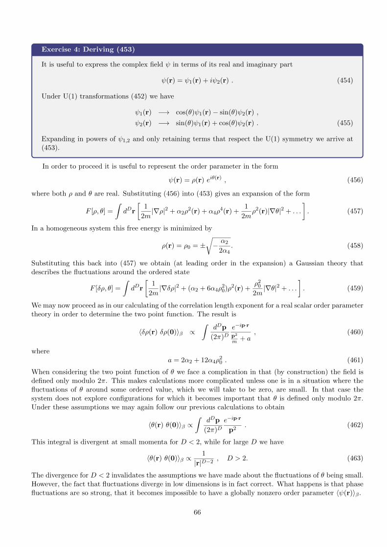
Exercise 4: Deriving (453)

It is useful to express the complex field ψ in terms of its real and imaginary part

ψ(r) = ψ1(r) + iψ2(r) . (454)

Under U(1) transformations (452) we have

ψ1(r) −→ cos(θ)ψ1(r)− sin(θ)ψ2(r) ,

ψ2(r) −→ sin(θ)ψ1(r) + cos(θ)ψ2(r) . (455)

Expanding in powers of ψ1,2 and only retaining terms that respect the U(1) symmetry we arrive at(453).

In order to proceed it is useful to represent the order parameter in the form

ψ(r) = ρ(r) eiθ(r) , (456)

where both ρ and θ are real. Substituting (456) into (453) gives an expansion of the form

F [ρ, θ] =

∫dDr

[1

2m|∇ρ|2 + α2ρ

2(r) + α4ρ4(r) +

1

2mρ2(r)|∇θ|2 + . . .

]. (457)

In a homogeneous system this free energy is minimized by

ρ(r) = ρ0 = ±√− α2

2α4. (458)

Substituting this back into (457) we obtain (at leading order in the expansion) a Gaussian theory thatdescribes the fluctuations around the ordered state

F [δρ, θ] =

∫dDr

[1

2m|∇δρ|2 + (α2 + 6α4ρ

20)ρ2(r) +

ρ20

2m|∇θ|2 + . . .

]. (459)

We may now proceed as in our calculating of the correlation length exponent for a real scalar order parametertheory in order to determine the two point function. The result is

〈δρ(r) δρ(0)〉β ∝∫

dDp

(2π)De−ip·r

p2

m + a, (460)

wherea = 2α2 + 12α4ρ

20 . (461)

When considering the two point function of θ we face a complication in that (by construction) the field isdefined only modulo 2π. This makes calculations more complicated unless one is in a situation where thefluctuations of θ around some ordered value, which we will take to be zero, are small. In that case thesystem does not explore configurations for which it becomes important that θ is defined only modulo 2π.Under these assumptions we may again follow our previous calculations to obtain

〈θ(r) θ(0)〉β ∝∫

dDp

(2π)De−ip·r

p2. (462)

This integral is divergent at small momenta for D < 2, while for large D we have

〈θ(r) θ(0)〉β ∝1

|r|D−2, D > 2. (463)

The divergence for D < 2 invalidates the assumptions we have made about the fluctuations of θ being small.However, the fact that fluctuations diverge in low dimensions is in fact correct. What happens is that phasefluctuations are so strong, that it becomes impossible to have a globally nonzero order parameter 〈ψ(r)〉β.

66

10 Regime of validity of the saddle point approximation/mean fieldtheory

An important question is how reliable the saddle-point approximation we have used to analyze path integralslike (381) is. A useful consistency check is obtained by comparing the variance of the order parameter toits square when averaged over a spatial region with a radius set by the correlation length ξ. The variancegives a measure of the size of the fluctuations around the average and for a translationally invariant systemis given by

〈(δφ)2〉Rξ =⟨[ ∫

Rξ

dDr(φ(r)− 〈φ(r)〉︸ ︷︷ ︸

δφ(r)

)]2⟩=

∫Rξ

dDr

∫Rξ

dDr′⟨δφ(r) δφ(r′)〉

∼∫Rξ

dDr

∫Rξ

dDr′ ξ3−D

2e−|r−r

′|/ξ

|r− r′|D−1

2

∝ ξ2+D. (464)

Here Rξ is a box of length ξ centered around the origin and we have used our result (434) for the two pointfunction in the Gaussian approximation. This should be compared to the square of the order parameteraveraged over Rξ

〈φ〉2Rξ = ξ2D〈φ(0)〉2 . (465)

We have〈(δφ)2〉Rξ〈φ〉2Rξ

∝ ξ2−D

〈φ(0)〉2∝ |t|ν(D−2)−2β, (466)

where ν and β are the correlation length and order parameter exponents respectively. The saddle pointapproximation has a chance of being accurate as long as the right hand side of (466) is much less than 1,which occurs if the exponent of |t| is positive. Using our previous results that β = ν = 1

2 we therefore require

D > 4. (467)

This means that our saddle point approximation is not expected to work quantitatively in dimensions lessthan 4. The dimension above which a saddle point (mean field) approximation becomes valid is called uppercritical dimension. In D < 4 a significantly more refined analysis based on the renormalization group isrequired to obtain quantitative results.

Mean field theory can fail in another way: at low temperatures it predicts an ordered phase, but we havealready seen for the case of the 1D Ising model and the Landau theory for a superfluid that in low numbers ofspatial dimensions fluctuations can be so strong that they preclude the formation of an ordered state. Thisfact goes under the name of “Mermin-Wagner-Hohenberg theorem”. The dimension below which there is noordered phase is called lower critical dimensions. As we have seen, the formation of order is associated withthe spontaneous breaking of a discrete (Z2 spin reflection for the Ising model) or continuous (spin rotationalsymmetry SU(2) for the Heisenberg model, U(1) for the superfluid) symmetry. For systems with sort rangeinteractions as the ones we have considered here, continuous symmetries can be broken spontaneously onlyat zero temperature in D = 2, and never in D = 1. In contrast, discrete symmetries can be broken onlyat zero temperature in D = 1. Let us summarize our findings for the example for the Landau theory of asuperfluid.

• For D > 4 the saddle point approximation is valid (the upper critical dimension is 4). There is atransition to an ordered phase and the critical exponents are given by mean field theory.

• In the intermediate regime 2 < D < 4 there is a transition to an ordered state at low temperatures,but fluctuations modify the mean-field behaviour and lead to different values for the critical exponentscharacterizing the phase transition.

67

• For D < 2 (the lower critical dimension is 2) phase fluctuations become so strong that it is no longerpossible for the system to order at low temperatures.

68