Lecture Notes for the C6 Theory Option

F.H.L. EsslerThe Rudolf Peierls Centre for Theoretical Physics

Oxford University, Oxford OX1 3NP, UK

May 11, 2016

Please report errors and typos to fab@thphys.ox.ac.ukc©2015 F.H.L. Essler

Contents

I Functional Methods in Quantum Mechanics 3

1 Some Mathematical Background 31.1 Functionals . . . . . . . . . . . . . . . . . . . . . . . . . . . . . . . . . . . . . . . . . . . . . 31.2 Functional differentiation . . . . . . . . . . . . . . . . . . . . . . . . . . . . . . . . . . . 41.3 Multidimensional Gaussian Integrals . . . . . . . . . . . . . . . . . . . . . . . . . . . . 61.4 Homework Questions 1&2 . . . . . . . . . . . . . . . . . . . . . . . . . . . . . . . . . . . . . . 7

2 Path Integrals in Quantum Mechanics 82.1 The Propagator . . . . . . . . . . . . . . . . . . . . . . . . . . . . . . . . . . . . . . . . . . 8

2.1.1 Propagator as a “Functional Integral” . . . . . . . . . . . . . . . . . . . . . . 102.2 Quantum Mechanics a la Feynman . . . . . . . . . . . . . . . . . . . . . . . . . . . . . . 112.3 Classical Limit and Stationary Phase Approximation . . . . . . . . . . . . . . . . . . 112.4 The Propagator for Free Particles . . . . . . . . . . . . . . . . . . . . . . . . . . . . . 112.5 Homework Questions 3-5 . . . . . . . . . . . . . . . . . . . . . . . . . . . . . . . . . . . . . . . 13

3 Path Integrals in Quantum Statistical Mechanics 153.1 Harmonic Oscillator at T > 0: a first encounter with Generating Functionals 16

3.1.1 Imaginary Time Green’s Function of the Harmonic Oscillator . . . . . . . 183.2 Homework Question 6 . . . . . . . . . . . . . . . . . . . . . . . . . . . . . . . . . . . . . . . . 193.3 Correlation Functions . . . . . . . . . . . . . . . . . . . . . . . . . . . . . . . . . . . . . 20

3.3.1 Wick’s Theorem . . . . . . . . . . . . . . . . . . . . . . . . . . . . . . . . . . . . . . 213.4 Probability distribution of position . . . . . . . . . . . . . . . . . . . . . . . . . . . . . 223.5 Perturbation Theory and Feynman Diagrams . . . . . . . . . . . . . . . . . . . . . . . 22

3.5.1 Partition Function of the anharmonic oscillator . . . . . . . . . . . . . . . 233.6 Homework Question 7 . . . . . . . . . . . . . . . . . . . . . . . . . . . . . . . . . . . . . . . . 25

II Path Integrals and Transfer Matrices 26

4 Relation of D dimensional quantum systems to D + 1 dimensional classical ones 264.1 Some Facts from Statistical Physics . . . . . . . . . . . . . . . . . . . . . . . . . . . . 264.2 Quantum Mechanical Particle . . . . . . . . . . . . . . . . . . . . . . . . . . . . . . . . 26

1

5 The Ising Model 285.1 Statistical mechanics of the Ising model . . . . . . . . . . . . . . . . . . . . . . . . . . 285.2 The One-Dimensional Ising Model . . . . . . . . . . . . . . . . . . . . . . . . . . . . . . 28

5.2.1 Transfer matrix approach . . . . . . . . . . . . . . . . . . . . . . . . . . . . . . . 295.2.2 Averages of observables in the transfer matrix formalism . . . . . . . . . . 305.2.3 The related zero-dimensional quantum model . . . . . . . . . . . . . . . . . . 31

5.3 The Two-Dimensional Ising Model . . . . . . . . . . . . . . . . . . . . . . . . . . . . . . 325.3.1 Transfer Matrix Method . . . . . . . . . . . . . . . . . . . . . . . . . . . . . . . . 325.3.2 Spontaneous Symmetry Breaking . . . . . . . . . . . . . . . . . . . . . . . . . . . 33

5.4 Homework Questions 8-10 . . . . . . . . . . . . . . . . . . . . . . . . . . . . . . . . . . . . . . 35

III Many-Particle Quantum Mechanics 37

6 Second Quantization 376.1 Systems of Independent Particles . . . . . . . . . . . . . . . . . . . . . . . . . . . . . . 37

6.1.1 Occupation Number Representation . . . . . . . . . . . . . . . . . . . . . . . . . 386.2 Fock Space . . . . . . . . . . . . . . . . . . . . . . . . . . . . . . . . . . . . . . . . . . . . . 39

6.2.1 Creation and Annihilation Operators . . . . . . . . . . . . . . . . . . . . . . . 396.2.2 Basis of the Fock Space . . . . . . . . . . . . . . . . . . . . . . . . . . . . . . . . . 40

6.3 Homework Questions 11-13 . . . . . . . . . . . . . . . . . . . . . . . . . . . . . . . . . . . . . 406.3.1 Change of Basis . . . . . . . . . . . . . . . . . . . . . . . . . . . . . . . . . . . . . . 41

6.4 Second Quantized Form of Operators . . . . . . . . . . . . . . . . . . . . . . . . . . . 426.4.1 Occupation number operators . . . . . . . . . . . . . . . . . . . . . . . . . . . . . 426.4.2 Single-particle operators . . . . . . . . . . . . . . . . . . . . . . . . . . . . . . . 426.4.3 Two-particle operators . . . . . . . . . . . . . . . . . . . . . . . . . . . . . . . . . 45

6.5 Homework Question 14 . . . . . . . . . . . . . . . . . . . . . . . . . . . . . . . . . . . . . . . 47

7 Application I: The Ideal Fermi Gas 487.1 Quantization in a large, finite volume . . . . . . . . . . . . . . . . . . . . . . . . . . . 48

7.1.1 Ground State . . . . . . . . . . . . . . . . . . . . . . . . . . . . . . . . . . . . . . . 497.1.2 Excitations . . . . . . . . . . . . . . . . . . . . . . . . . . . . . . . . . . . . . . . . . 507.1.3 Density Correlations . . . . . . . . . . . . . . . . . . . . . . . . . . . . . . . . . . 50

7.2 Homework Questions 15-16 . . . . . . . . . . . . . . . . . . . . . . . . . . . . . . . . . . . . . 53

8 Application II: Weakly Interacting Bosons 548.1 Ideal Bose Gas . . . . . . . . . . . . . . . . . . . . . . . . . . . . . . . . . . . . . . . . . . . 558.2 Bogoliubov Approximation . . . . . . . . . . . . . . . . . . . . . . . . . . . . . . . . . . . 558.3 Bogoliubov Transformation . . . . . . . . . . . . . . . . . . . . . . . . . . . . . . . . . . 568.4 Ground State and Low-lying Excitations . . . . . . . . . . . . . . . . . . . . . . . . . 578.5 Ground state correlation functions . . . . . . . . . . . . . . . . . . . . . . . . . . . . 588.6 Depletion of the Condensate . . . . . . . . . . . . . . . . . . . . . . . . . . . . . . . . . 59

9 Application III: Spinwaves in a Ferromagnet 599.1 Heisenberg model and spin-rotational SU(2) symmetry . . . . . . . . . . . . . . . . . 609.2 Exact ground states . . . . . . . . . . . . . . . . . . . . . . . . . . . . . . . . . . . . . . . 609.3 Spontaneous Symmetry Breaking . . . . . . . . . . . . . . . . . . . . . . . . . . . . . . . 619.4 Holstein-Primakoff Transformation . . . . . . . . . . . . . . . . . . . . . . . . . . . . 62

9.4.1 Heisenberg Antiferromagnet . . . . . . . . . . . . . . . . . . . . . . . . . . . . . 639.5 Homework Questions 17-18 . . . . . . . . . . . . . . . . . . . . . . . . . . . . . . . . . . . . . 63

2

10 Path Integral for interacting Bose systems 6410.1 Coherent States . . . . . . . . . . . . . . . . . . . . . . . . . . . . . . . . . . . . . . . . . . 6510.2 Partition Function . . . . . . . . . . . . . . . . . . . . . . . . . . . . . . . . . . . . . . . . 66

Part I

Functional Methods in Quantum Mechanics

1 Some Mathematical Background

Functional Methods form a central part of modern theoretical physics. In the following we introduce thenotion of functionals and how to manipulate them.

1.1 Functionals

What is a functional? You all know that a real function can be viewed as a map from e.g. an interval [a, b]to the real numbers

f : [a, b]→ R , x→ f(x). (1)

A functional is similar to a function in that it maps all elements in a certain domain to real numbers,however, the nature of its domain is very different. Instead of acting on all points of an interval or someother subset of the real numbers, the domain of functionals consists of (suitably chosen) classes of functions.In other words, given some class {f} of functions, a functional F is a map

F : {f} → R , f → F [f ]. (2)

We now consider two specific examples of functionals.

1. The distance between two points. A very simple functional F consists of the map which assigns to allpaths between two fixed points the length of the path. To write this functional explicitly, let us considera simple two-dimensional situation in the (x, y) plane and choose two points (x1, y1) and (x2, y2). Weconsider the set of paths that do not turn back, i.e. paths along which x increases monotonically as wego from (x1, y1) to (x2, y2). These can be described by the set of functions {f} on the interval [x1, x2]satisfying f(x1) = y1 and f(x2) = y2. The length of a path is then given by the well-known expression

F [f(x)] =

∫ x2

x1

dx′√

1 + f ′(x′)2 . (3)

2. Action Functionals. These are very important in Physics. Let us recall their definition in the contextof classical mechanics. Start with n generalised coordinates q(t) = (q1(t), . . . , qn(t)) and a LagrangianL = L(q, q). Then, the action functional S[q] is defined by

S[q] =

∫ t2

t1

dtL(q(t), q(t)) . (4)

It depends on classical paths q(t) between times t1 and t2 satisfying the boundary conditions q(t1) = q1

and q(t2) = q2.

3

1.2 Functional differentiation

In both the examples given above a very natural question to ask is what function extremizes the functional.In the first example this corresponds to wanting to know the path that minimizes the distance between twopoints. In the second example the extremum of the action functional gives the solutions to the classicalequations of motion. This is known as Hamilton’s principle. In order to figure out what function extremizesthe functional it is very useful to generalize the notion of a derivative. For our purposes we define thefunctional derivative by

δF [f(x)]

δf(y)= lim

ε→0

F [f(x) + εδ(x− y)]− F [f(x)]

ε.

(5)

Here, as usual, we should think of the δ-function as being defined as the limit of a test function, e.g.

δ(x) = lima→0

1√πae−x

2/a2 , (6)

and take the limit a → 0 only in the end (after commuting the limit with all other operations such asthe limε→0 in (5)). Importantly, the derivative defined in this way is a linear operation which satisfies theproduct and chain rules of ordinary differentiation and commutes with ordinary integrals and derivatives.Let us see how functional differentiation works for our two examples.

1. The distance between two points. In analogy with finding stationary points of functions we want toextremize (3) by setting its functional derivative equal to zero

0 =δF [f(x)]

δf(y). (7)

We first do the calculation by using the definition (5).

δF [f(x)]

δf(y)= lim

ε→0

∫ x2

x1

dx′

√1 + [f ′(x′) + εδ′(x′ − y)]2 −

√1 + [f ′(x′)]2

ε. (8)

The Taylor expansion of the square root is√

1 + 2ε = 1 + ε+ . . ., which gives√1 + [f ′(x′) + εδ′(x′ − y)]2 =

√1 + [f ′(x′)]2 +

εf ′(x′)δ′(x′ − y)√1 + [f ′(x′)]2

+O(ε2) , (9)

where δ′(x) is the derivative of the delta-function and O(ε2) denote terms proportional to ε2. Substi-tuting this back into (8) we have 1

δF [f(x)]

δf(y)=

∫ x2

x1

dx′δ′(x′ − y)f ′(x′)√

1 + [f ′(x′)]2= − d

dy

f ′(y)√1 + [f ′(y)]2

. (11)

The solution to (7) is thusf ′(y) = const, (12)

which describes a straight line. In practice we don’t really go back to the definition of the functionalderivative any more than we use the definition of an ordinary derivative to work it out, but proceedas follows.

1In the last step we have used ∫ b

a

dx′δ′(x′ − y)g(x′) = −g′(y) , (10)

which can be proved by “integration by parts”.

4

• We first interchange the functional derivative and the integration

δF [f(x)]

δf(y)=

∫ x2

x1

dx′δ

δf(y)

√1 + [f ′(x′)]2. (13)

• Next we use the chain rule

δ√

1 + f ′(x′)2

δf(y)=

1

2√

1 + f ′(x′)2

δ(1 + f ′(x′)2)

δf(y)=

f ′(x′)√1 + f ′(x′)2

δf ′(x′)

δf(y). (14)

• Finally we interchange the functional and the ordinary derivative

δf ′(x′)

δf(y)=

d

dx′δf(x′)

δf(y)=

d

dx′δ(x′ − y) . (15)

The last identity follows from our definition (5).

Now we can put everything together and arrive at the same answer (11).

Exercise

2. Next we want to try out these ideas on our second example and extremize the classical action (4) in orderto obtain the classical equations of motion. We first interchange functional derivative and integration andthen use the chain rule to obtain

δS[q]

δqi(t)=

δ

δqi(t)

∫ t2

t1

dt L(q(t), q(t)) (16)

=

∫ t2

t1

dt

[∂L

∂qj(q, q)

δqj(t)

δqi(t)+∂L

∂qj(q, q)

δqj(t)

δqi(t)

](17)

(18)

We now use thatδqj(t)δqi(t)

= ddt

δqj(t)δqi(t)

and integrate by parts with respect to t

δS[q]

δqi(t)=

∫ t2

t1

dt

[∂L

∂qj(q, q)− d

dt

∂L

∂qj(q, q)

]δqj(t)

δqi(t)(19)

=

∫ t2

t1

dt

[∂L

∂qj(q, q)− d

dt

∂L

∂qj(q, q)

]δijδ(t− t) =

∂L

∂qi(q, q)− d

dt

∂L

∂qi(q, q) . (20)

In the second last step we have usedδqj(t)

δqi(t)= δijδ(t− t) , (21)

which follows straightforwardly from our general definition (5). Thus we conclude that the extrema of theclassical action are given by paths that fulfil the equations of motion

∂L

∂qi(q, q)− d

dt

∂L

∂qi(q, q) = 0.

(22)

Nice.

Exercise

5

1.3 Multidimensional Gaussian Integrals

As a reminder, we start with a simple one-dimensional Gaussian integral over a single variable y. It is givenby

I(z) ≡∫ ∞−∞

dy exp(−1

2zy2) =

√2π

z,

(23)

where z is a complex number with Re(z) > 0. The standard proof of this relation involves writing I(z)2

as a two-dimensional integral over y1 and y2 and then introducing two-dimensional polar coordinates r =√y2

1 + y22 and ϕ. Explicitly,

I(z)2 =

∫ ∞−∞

dy1 exp(−1

2zy2

1)

∫ ∞−∞

dy2 exp(−1

2zy2

2) =

∫ ∞−∞

dy1

∫ ∞−∞

dy2 exp(−1

2z(y2

1 + y22)) (24)

=

∫ 2π

0dϕ

∫ ∞0

dr r exp(−1

2zr2) =

2π

z. (25)

Next we consider n-dimensional Gaussian integrals

W0(A) ≡∫dny exp

(−1

2yTAy

), (26)

over variables y = (y1, . . . , yn), where A is a symmetric, positive definite matrix (all its eigenvalues arepositive). This integral can be reduced to a product of one-dimensional Gaussian integrals by diagonalisingthe matrix A. Consider an orthogonal rotation O such that A = ODOT with a diagonal matrix D =diag(a1, . . . , an). The eigenvalues ai are strictly positive since we have assumed that A is positive definite.Introducing new coordinates y = OTy we can write

yTAy = yTDy =

n∑i=1

aiy2i , (27)

where the property OTO = 1 of orthogonal matrices has been used. Note further that the Jacobian ofthe coordinate change y → y is one, since |det(O)| = 1. Hence, using Eqs. (23) and (27) we find for theintegral (26)

W0(A) =

n∏i=1

∫dyi exp(−1

2aiy

2i ) = (2π)n/2(a1a2 . . . an)−1/2 = (2π)n/2(detA)−1/2 . (28)

To summarise, we have found for the multidimensional Gaussian integral (26) that

W0(A) = (2π)n/2(detA)−1/2 ,(29)

a result which will be of some importance in the following. We note that if we multiply the matrix A by acomplex number z with Re(z) > 0 and then follow through exactly the same steps, we find

W0(zA) =

(2π

z

)n/2(detA)−1/2 . (30)

One obvious generalisation of the integral (26) involves adding a term linear in y in the exponent, that is

W0(A,J) ≡∫dny exp

(−1

2yTAy + JTy

). (31)

6

Here J = (J1, . . . , Jn) is an n-dimensional vector. Changing variables y→ y, where

y = A−1J + y (32)

this integral can be written as

W0(A,J) = exp

(1

2JTA−1J

)∫dny exp

(−1

2yTAy

). (33)

The remaining integral is Gaussian without a linear term, so can be easily carried out using the aboveresults. Hence, one finds

W0(A,J) = (2π)n/2(detA)−1/2 exp

(1

2JTA−1J

).

(34)

1.4 Homework Questions 1&2

Question 1. Consider paths X = X(τ), where τ is a parameter, and the functional

l[X] =

∫ τ1

τ0

dτ n(X)

√dX

dτ· dXdτ

,

where n = n(X) is a function. (The minima of this functional can be interpreted as light rays propagating in amedium with refractive index n.)a) Derive the differential equation which has to be satisfied by minimal paths X.b) Consider a two-dimensional situation with paths X(τ) = (X(τ), Y (τ)) in the x, y plane and a functionn = n0 + (n1 − n0) θ(x). (The Heaviside function θ(x) is defined to be 0 for x < 0 and 1 for x ≥ 0. Recallthat θ′(x) = δ(x).) Solve the differential equation in a) for this situation, using the coordinate x as parameter τalong the path.c) Show that the solution in b) leads to the standard law for refraction at the boundary between two media withrefractive indices n0 and n1.

Question 2. a) Evaluate the Gaussian integral∫ ∞−∞

dx e−12zx2 (35)

for a complex constant z. What is the requirement on z for the integral to exist?b) The gamma function Γ is defined by

Γ(s+ 1) =

∫ ∞0

dxxse−x .

c) Show that Γ(1) = 1 and Γ(s+ 1) = sΓ(s). (Hence Γ(n+ 1) = n!)d) Take s to be real and positive. Evaluate Γ(s+ 1) in the steepest descent approximation: write the integrandin the form ef(x) and argue that for large s� 1 the dominant contribution to the integral arises from the minimaof f(x). Expand the function to quadratic order around the minimum, argue that you may extend the integrationboundaries to ±∞, and then carry out the resulting integral. Your result is known as Stirling’s approximation: ittells you what n! is when n becomes large.e)∗ The following extension is for complex analysis afficionados, so simply omit it if you haven’t taken the shortoption. Take s to be complex with positive real part. Deform the contour in a suitable way, so that you canagain apply a steepest descent approximation. Ponder the name of the method. What is Stirling’s approximationfor complex s?

7

2 Path Integrals in Quantum Mechanics

So far you have encountered two ways of doing QM:

1. Following Schrodinger, we can solve the Schrodinger equation for the wave function → Fun withPDEs...

2. Following Heisenberg, we can work with operators, commutation relations, eigenstates → Fun withLinear Algebra...

Historically it took some time for people to realize that these are in fact equivalent. To quote the greatmen: I knew of Heisenberg’s theory, of course, but I felt discouraged, not to say repelled, by the methodsof transcendental algebra, which appeared difficult to me, and by the lack of visualizability. (Schrodinger in1926)

The more I think about the physical portion of Schrodinger’s theory, the more repulsive I find it. WhatSchrodinger writes about the visualizability of his theory is probably not quite right, in other words it’s crap.(Heisenberg, writing to Pauli in 1926)

There is a third approach to QM, due to Feynman. He developed it when he was a graduate student,inspired by a mysterious remark in a paper by Dirac. Those were the days! Feynman’s approach is partic-ularly useful for QFTs and many-particle QM problems, as it makes certain calculations much easier. Wewill now introduce it by working backwards. The central object in Feynman’s method is something calleda propagator. We’ll now work out what this is using the Heisenberg/Schrodinger formulation of QM youknow and love. After we have done that, we formulate QM a la Feynman.

2.1 The Propagator

Our starting point is the time-dependent Schrodinger equation

i~∂

∂t|ψ(t)〉 = H|ψ(t)〉. (36)

We recall that the wave function is given by

ψ(~x, t) = 〈~x|ψ(t)〉. (37)

Eqn (36) can be integrated to give

|ψ(t)〉 = e−i~Ht|ψ(0)〉 (38)

The time-evolution operator in QM is thus (assuming that H is time-independent)

U(t; t0) = e−i~H(t−t0). (39)

A central object in Feynman’s approach is the propagator

〈~x′|U(t; t0)|~x〉,(40)

where |~x〉 are the simultaneous eigenstates of the position operators x, y and z. The propagator is theprobability amplitude for finding our QM particle at position ~x′ at time t, if it started at position ~x at timet0. To keep notations simple, we now consider a particle moving in one dimension with time-independentHamiltonian

H = T + V =p2

2m+ V (x). (41)

We want to calculate the propagator〈xN |U(t; 0)|x0〉. (42)

8

It is useful to introduce small time steps

tn = nε , n = 0, . . . , N, (43)

where ε = t/N . Then we have by construction

U(t; 0) =(e−

i~Hε)N

. (44)

The propagator is

〈xN |U(t; 0)|x0〉 = 〈xN |e−i~Hε · · · e−

i~Hε|x0〉

=

∫dxN−1 . . .

∫dx1 〈xN |e−

i~Hε|xN−1〉〈xN−1|e−

i~Hε|xN−2〉 . . . 〈x1|e−

i~Hε|x0〉, (45)

where we have inserted N − 1 resolutions of the identity in terms of position eigenstates

1 =

∫dx |x〉〈x| . (46)

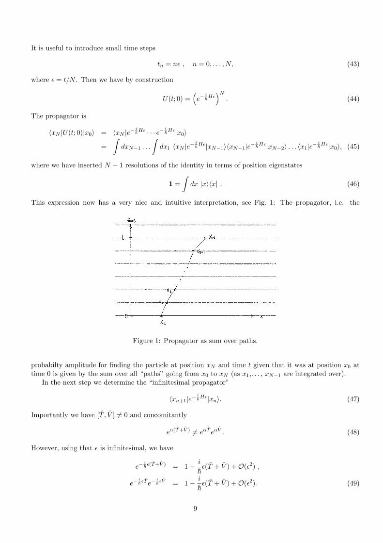
This expression now has a very nice and intuitive interpretation, see Fig. 1: The propagator, i.e. the

Figure 1: Propagator as sum over paths.

probabilty amplitude for finding the particle at position xN and time t given that it was at position x0 attime 0 is given by the sum over all “paths” going from x0 to xN (as x1,. . . , xN−1 are integrated over).

In the next step we determine the “infinitesimal propagator”

〈xn+1|e−i~Hε|xn〉. (47)

Importantly we have [T , V ] 6= 0 and concomitantly

eα(T+V ) 6= eαT eαV . (48)

However, using that ε is infinitesimal, we have

e−i~ ε(T+V ) = 1− i

~ε(T + V ) +O(ε2) ,

e−i~ εT e−

i~ εV = 1− i

~ε(T + V ) +O(ε2). (49)

9

So up to terms of order ε2 we have

〈xn+1|e−i~Hε|xn〉 ' 〈xn+1|e−

i~ T εe−

i~ V ε|xn〉 = 〈xn+1|e−

i~ T ε|xn〉e−

i~V (xn)ε, (50)

where we have used that V |x〉 = V (x)|x〉. As T = p2/2m it is useful to insert a complete set of momentumeigenstates 2 to calculate

〈xn+1|e−i~ T ε|xn〉 =

∫dp

2π~〈xn+1|e−

ip2ε2m~ |p〉〈p|xn〉 =

∫dp

2π~e−

ip2ε2m~−i

p~ (xn−xn+1)

=

√m

2πi~εeim2~ε (xn−xn+1)2 . (51)

In the second step we have used that p|p〉 = p|p〉 and that

〈x|p〉 = eipx~ . (52)

The integral over p is performed by changing variables to p′ = p + mε (xn − xn+1) (and giving ε a very

small imaginary part in order to make the integral convergent). Substituting (51) and (50) back into ourexpression (45) for the propagator gives

〈xN |U(t; 0)|x0〉 = limN→∞

[ m

2πi~ε

]N2

∫dx1 . . . dxN−1 exp

(iε

~

N−1∑n=0

m

2

(xn+1 − xn

ε

)2

− V (xn)

). (53)

Note that in this expression there are no operators left.

2.1.1 Propagator as a “Functional Integral”

The way to think about (53) is as a sum over trajectories:

• x0, . . . , xN constitute a discretization of a path x(t′), where we set xn ≡ x(tn).

• We then havexn+1 − xn

ε=x(tn+1)− x(tn)

tn+1 − tn' x(tn), (54)

and

εN−1∑n=0

m

2

(xn+1 − xn

ε

)2

− V (xn) '∫ t

0dt′[m

2x2(t′)− V (x)

]≡∫ t

0dt′L[x, x], (55)

where L is the Lagrangian of the system. In classical mechanics the time-integral of the Lagrangianis known as the action

S =

∫ t

0dt′L. (56)

• The integral over x1, . . . xN−1 becomes a functional integral, also known as a path integral, over allpaths x(t′) that start at x0 at time t′ = 0 and end at xN at time t′ = t.

• The prefactor in (53) gives rise to an overall (infinite) normalization and we will denote it by N .

These considerations lead us to express the propagator as the following formal expression

〈xN |U(t; 0)|x0〉 = N∫Dx(t′) e

i~S[x(t′)].

(57)

What is in fact meant by (57) is the limit of the discretized expression (53). The ultimate utility of (57) isthat it provides a compact notation, that on the one hand will allow us to manipulate functional integrals,and on the other hand provides a nice, intuitive interpretation.

2We use a normalization 〈p|k〉 = 2π~δ(p− k), so that 1 =∫

dp2π~ |p〉〈p|.

10

2.2 Quantum Mechanics a la Feynman

Feynman’s formulation of Quantum Mechanics is based on the single postulate that the probability amplitudefor propagation from a position x0 to a position xN is obtained by summing over all possible paths connectingx0 and xN , where each path is weighted by a phase factor exp

(i~S), where S is the classical action of the

path. This provides a new way of thinking about QM!

2.3 Classical Limit and Stationary Phase Approximation

An important feature of (57) is that it gives us a nice way of thinking about the classical limit “~→ 0” (moreprecisely in the limit when the dimensions, masses, times etc are so large that the action is huge comparedto ~). To see what happens in this limit let us first consider the simpler case of an ordinary integral

g(a) =

∫ ∞−∞

dt h1(t)eiah2(t), (58)

when we take the real parameter a to infinity. In this case the integrand will oscillate wildly as a function oft because the phase of exp

(iah2(t)

)will vary rapidly. The dominant contribution will arise from the points

where the phase changes slowly, which are the stationary points

h′2(t) = 0. (59)

The integral can then be approximated by expanding around the stationary points. Assuming that there isa single stationary point at t0

g(a� 1) ≈∫ ∞−∞

dt[h1(t0) + (t− t0)h′1(t0) + . . .

]eiah2(t0)+i

ah′′2 (t0)

2(t−t0)2 , (60)

Changing integration variables to t′ = t − t0 (and giving a a small imaginary part to make the integralconverge at infinity) as obtain a Gaussian integral that we can take using (23)

g(a� 1) ≈

√2πi

ah′′2(t0)h1(t0)eiah2(t0) . (61)

Subleading contributions can be evaluated by taking higher order contributions in the Taylor expansionsinto account. If we have several stationary points we sum over their contributions. The method we havejust discussed is known as stationary phase approximation.

The generalization to path integrals is now clear: in the limit ~ → 0 the path integral is dominated bythe vicinity of the stationary points of the action S

δS

δx(t′)= 0. (62)

The condition (62) precisely defines the classical trajectories x(t′)!

2.4 The Propagator for Free Particles

We now wish to calculate the functional integral (57) for a free particle, i.e.

V (x) = 0. (63)

Going back to the explicit expression (53) we have

〈xN |U(t; 0)|x0〉 = limN→∞

[ m

2πi~ε

]N2

∫dx1 . . . dxN−1 exp

(iε

~

N−1∑n=0

m

2

(xn+1 − xn

ε

)2). (64)

11

It is useful to change integration variables to

yj = xj − xN , j = 1, . . . , N − 1, (65)

which leads to an expression

〈xN |U(t; 0)|x0〉 = limN→∞

[ m

2πi~ε

]N2

∫dy exp

(−1

2yTAy + JT · y

)eim2~ε (x0−xN )2 . (66)

Here

JT =( im~ε

(xN − x0), 0, . . . , 0), (67)

and A is a (N − 1)× (N − 1) matrix with elements

Ajk =−imε~

[2δj,k − δj,k+1 − δj,k−1] . (68)

For a given N (66) is a multidimensional Gaussian integral and can be carried out using (34)

〈xN |U(t; 0)|x0〉 = limN→∞

[ m

2πi~ε

]N2

(2π)N−1

2 [det(A)]−12 exp

(1

2JTA−1J

)eim2~ε (x0−xN )2 . (69)

The matrix A is related to the one dimensional lattice Laplacian, see below. Given the eigenvalues andeigenvectors worked out below we can calculate the determinant and inverse of A (homework problem).Substituting the results into (69) gives

〈xN |U(t; 0)|x0〉 =√

m2πi~te

im2~t (x0−xN )2 .

(70)

For a free particle we can evaluate the propagator directly in a much simpler way.

〈xN |U(t; 0)|x0〉 =

∫ ∞−∞

dp

2π~〈xN |e−i

p2t2m~ |p〉〈p|x0〉 =

∫ ∞−∞

dp

2π~e−i

p2t2m~−i

p(x0−xN )

~

=

√m

2πi~teim2~t (x0−xN )2 . (71)

Aside: Lattice Laplacian

The matrix A is related to the one dimensional Lattice Laplacian. Consider functions of a variable z0 ≤ z ≤ zNwith “hard-wall boundary conditions”

f(z0) = f(zN ) = 0. (72)

The Laplace operator D acts on these functions as

Df ≡ d2f(z)

dz2. (73)

Discretizing the variable z by introducing N − 1 points

zn = z0 + na0 , n = 1, . . . , N − 1 (74)

where a0 = (zN − z0)/N is a “lattice spacing”, maps the function f(z) to a N − 1 dimensional vector

f(z)→ f = (f(z1), . . . , f(zN−1)). (75)

Recalling thatd2f

dz2(z) = lim

a0→0

f(z + a0) + f(z − a0)− 2f(z)

a20

, (76)

12

we conclude that the Lapacian is discretized as follows

Df → a−20 ∆f , (77)

where∆jk = δj,k+1 + δj,k−1 − 2δj,k. (78)

Our matrix A is equal to imε~ ∆. The eigenvalue equation

∆an = λnan, n = 1, . . . , N − 1 (79)

gives rise to a recurrence relation for the components an,j of an

an,j+1 + an,j−1 − (2 + λn)an,j = 0. (80)

The boundary conditions an,N = an,0 = 0 suggest the ansatz

an,j = Cn sin(πnjN

). (81)

Substituting this in to (80) gives

λn = 2 cos(πnN

)− 2 , n = 1, . . . , N − 1. (82)

The normalized eigenvectors of ∆ are

an =1√∑N−1

j=1 sin2(πnjN

)

sin(πnN

)sin(

2πnN

)...

sin(π(N−1)n

N

).

=

√2

N

sin(πnN

)sin(

2πnN

)...

sin(π(N−1)n

N

).

(83)

Aside: Lattice Laplacian

2.5 Homework Questions 3-5

Question 3. Consider a free quantum mechanical particle moving in one dimension. The Hamiltonian is

H = − ~2

2m

d2

dx2. (84)

We have shown in the lecture that the propagator can be represented in the form

〈xN |e−i~ tH |x0〉 = lim

N→∞

[ m

2πi~ε

]N2

∫dx1 . . . dxN−1 exp

(iε

~

N−1∑n=0

m

2

(xn+1 − xn

ε

)2). (85)

a) Change variables from xj to yj = xj − xN to bring it to the form

〈xN |e−i~ tH |x0〉 = lim

N→∞

[ m

2πi~ε

]N2

∫dy exp

(−1

2yTAy + JT · y

)eim2~ε (x0−xN )2 . (86)

Give expressions for J and A.b) Carry out the integrals over yj to get an expression for the propagator in terms of A and J.c) Work out the eigenvalues λn and eigenvectors an of the matrix A. You may find helpful hints in the lecturenotes.d) What is det(A)? A useful identity you may use is

N−1∏j=1

2 sin(πj/2N) =√N. (87)

13

Now work out JTA−1J by working in the eigenbasis of A−1 (Hint: write this as JTA−1J = JTOTOA−1OTOJ,where OTO = 1 and OA−1OT is a diagonal matrix you have already calculated above.). A useful identity youmay use is

N−1∑j=1

cos2(πj/2N) =N − 1

2. (88)

e) Use the result you have obtained to write an explicit expression for the propagator.

Question 4. Denote the propagator by

K(t, x; t′x′) = 〈x|e−i~H(t−t′)|x′〉. (89)

Show that the wave function ψ(t, x) = 〈x|Ψ(t)〉, where |Ψ(t)〉 is a solution to the time-dependent Schrodingerequation

i~∂

∂t|Ψ(t)〉 = H|Ψ(t)〉, (90)

fulfils the integral equation

ψ(t, x) =

∫ ∞−∞

dx′ K(t, x; t′x′) ψ(t′, x′). (91)

Question 5. Diffraction through a slit. A free particle starting at x = 0 when t = 0 is determined topass between x0− b and x0 + b at time T . We wish to calculate the probabilty of finding the particle at positionx at time t = T + τ .a) Argue on the basis of Qu 5. that the (un-normalized) wave function can be written in the form

ψ(T + τ, x) =

∫ b

−bdy K(T + τ, x;T, x0 + y) K(T, x0 + y; 0, 0) , (92)

whereK(t, x; t′x′) = 〈x|e−

i~H(t−t′)|x′〉. (93)

b) Using that the propagation for 0 ≤ t < T and T ≤ t < T + τ is that of a free particle, obtain an explicitintegral representation for the wave function.c) Show that the wave function can be expressed in terms of the Fresnel integrals

C(x) =

∫ x

0dy cos(πy2/2) , S(x) =

∫ x

0dy sin(πy2/2) . (94)

Hint: make a substitution z = αy + β with suitably chosen α and β.Derive an expression for the ratio P (T + τ, x)/P (T + τ, x0), where P (T + τ, x)dx is the probability of finding

the particle in the interval [x, x+ dx] at time T + τ .d)∗ If you can get hold of Mathematica (the default assumption is that you will not), plot the result as a functionof the dimensionless parameter x/[b(1 + τ/T )] for x0 = 0 and different values of the ratio

γ =mb2(1 + τ/T )

~τ. (95)

Discuss your findings.

14

3 Path Integrals in Quantum Statistical Mechanics

Path integrals can also be used to describe quantum systems at finite temperatures. To see how this workswe now consider a quantum mechanical particle coupled to a heat bath at a temperature T . An importantquantity in Statistical Mechanics is the partition function

Z(β) = Tr[e−βH

], (96)

where H is the Hamiltonian of the system, Tr denotes the trace over the Hilbert space of quantum mechanicalstates, and

β =1

kBT. (97)

Ensemble averages of the quantum mechanical observable O are given by

〈O〉β =1

Z(β)Tr[e−βHO

]. (98)

Taking the trace over a basis of eigenstates of H with H|n〉 = En|n〉 gives

〈O〉β =1

Z(β)

∑n

e−βEn〈n|O|n〉 ,

Z(β) =∑n

e−βEn . (99)

Assuming that the ground state of H is non-degenerate we have

limT→0〈O〉β = 〈0|O|0〉 , (100)

where |0〉 is the ground state of the system. Let us consider a QM particle with Hamiltonian

H =p2

2m+ V (x), (101)

coupled to a heat bath at temperature T . The partition function can be written in a basis of positioneigenstates

Z(β) =

∫dx〈x|e−βH |x〉 =

∫dx

∫dx′ 〈x|x′〉 〈x′|e−βH |x〉. (102)

Here〈x′|e−βH |x〉 (103)

is very similar to the propagator

〈x′|e−i(t−t0)

~ H |x〉. (104)

Formally (103) can be viewed as the propagator in imaginary time τ = it, where we consider propagationfrom τ = 0 to τ = β~. Using this interpretation we can follow through precisely the same steps as beforeand obtain

〈xN |e−βH |x0〉 = limN→∞

[ m

2π~ε

]N2

∫dx1 . . . dxN−1 exp

(− ε~

N−1∑n=0

m

2

(xn+1 − xn

ε

)2

+ V (xn)

), (105)

where now

ε =~βN. (106)

15

We again can interpret this in terms of a sum over paths x(τ) with

x(τn) = xn , τn = nε. (107)

Going over to a continuum description we arrive at an imaginary-time functional integral

〈xN |e−βH |x0〉 = N∫Dx(τ) e−

1~SE [x(τ)],

(108)

where SE is called Euclidean action

SE [x(τ)] =

∫ ~β

0dτ

[m

2

(dx

dτ

)2

+ V (x)

], (109)

and the path integral is over all paths that start at x0 and end at xN . Substituting (108) into the expressionfor the partition function we find that

Z(β) = N∫Dx(τ) e−

1~SE [x(τ)],

(110)

where we integrate over all periodic pathsx(~β) = x(0). (111)

The restriction to periodic paths arises because Z(β) is a trace. Please note that the notation∫Dx(τ)

means very different things in (108) and (110), as a result of involving very different classes of paths thatare “integrated over”. In the first case the path integral is over all paths from x0 to xN , in the latter over allperiodic paths starting an an arbitrary position. In practice it is always clear from the context what pathsare involved, and hence this ambiguous notation should not cause any confusion.

3.1 Harmonic Oscillator at T > 0: a first encounter with Generating Functionals

We now consider the simplest case of the potential V (x), the harmonic oscillator

H =p2

2m+κ

2x2. (112)

The physical quantities we want to work out are the averages of powers of the position operator

〈xn〉β =

∫dx 〈x|e−βH xn|x〉∫dx〈x|e−βH |x〉

=

∫dx xn 〈x|e−βH |x〉∫dx〈x|e−βH |x〉

. (113)

If we know all these moments, we can work out the probability distribution for a position measurementgiving a particular result x. At zero temperature this is just given by the absolute value squared of theground state wave function. The coupling to the heat bath will generate “excitations” of the harmonicoscillator and thus affect this probability distribution. We have

〈x|e−βH |x〉 = N∫Dx(τ) e

− 1~∫ ~β0 dτ

[m2 ( dxdτ )

2+κ

2x2

], (114)

where the path integral is over all paths with x(0) = x(β~). Integrating by parts we can write the action as

−1

~SE [x(τ)] = −1

~

∫ ~β

0dτ

[m

2

(dx

dτ

)2

+κ

2x2

]= −1

2

∫ ~β

0dτ x(τ)Dx(τ)− m

2~x(τ)x(τ)

∣∣∣~β0, (115)

where

D = −m~d2

dτ2+κ

~. (116)

16

The contributions from the integration boundaries in (115) don’t play a role in the logic underlying thefollowing steps leading up to (124) and work out in precisely the same way as the “bulk” contributions. Inorder to show that we’re not dropping anything important we’ll keep track of them anyway. We now definethe generating functional

W [J ] ≡ N∫Dx(τ) e−

1~SE [x(τ)]+

∫ ~β0 dτ J(τ)x(τ). (117)

Here the functions J(τ) are called sources. The point of the definition (117) is that we can obtain 〈xn〉β bytaking functional derivatives

〈xn〉β =1

W [0]

δ

δJ(0). . .

δ

δJ(0)

∣∣∣∣∣J=0

W [J ]. (118)

We now could go ahead and calculate the generating functional by going back to the definition of the thepath integral in terms of a multidimensional Gaussian integral. In practice we manipulate the path integralitself as follows. Apart from the contribution from the integration boundaries the structure of (115) iscompletely analogous to the one we encountered for Gaussian integrals, cf (31). The change of variables(32) suggests that we should shift our “integration variables” by a term involving the inverse of the integraloperator D. The latter corresponds to the Green’s function defined by

DτG(τ − τ ′) = δ(τ − τ ′) , G(0) = G(β~). (119)

We then change variables in the path integral in order to “complete the square”

y(τ) = x(τ)−∫dτ ′ G(τ − τ ′)J(τ ′). (120)

Under this change of variables we have∫dτ x(τ)Dτx(τ)− 2

∫dτ x(τ)J(τ) =

∫dτ y(τ)Dτy(τ)−

∫dτdτ ′ J(τ)G(τ − τ ′)J(τ ′)

+boundary terms. (121)

ExerciseVerify that∫

dτ y(τ)Dτy(τ) =

∫dτ x(τ)Dτx(τ) +

∫dτdτ ′dτ ′′ G(τ − τ ′)J(τ ′)DτG(τ − τ ′′)J(τ ′′)

−∫dτdτ ′

[x(τ)DτG(τ − τ ′)J(τ ′) +G(τ − τ ′)J(τ ′)Dτx(τ)

]=

∫dτ x(τ)Dτx(τ) +

∫dτdτ ′ G(τ − τ ′)J(τ ′)J(τ)− 2

∫dτ x(τ)J(τ)

+m

~x(τ)x(τ)

∣∣∣~β0− m

~y(τ)y(τ)

∣∣∣~β0, (122)

In the last step you need to use (119) and integrate by parts twice to simplify the last term in the second line.

Exercise

Putting everything together we arrive at

−1

~SE [x(τ)] +

∫ ~β

0dτ J(τ)x(τ) = −1

~SE [y(τ)] +

1

2

∫ ~β

0dτdτ ′J(τ)G(τ − τ ′)J(τ ′). (123)

On the other hand, the Jacobian of the change of variables (120) is 1 as we are shifting all paths by thesame constant (you can show this directly by going back to the definition of the path integral in terms ofmultiple Gaussian integrals). Hence we have Dy(τ) = Dx(τ) and our generating functional becomes

W [J ] = W [0] e12

∫dτdτ ′ J(τ)G(τ−τ ′)J(τ ′).

(124)

17

Now we are ready to calculate (118). The average position is zero

〈x〉β =1

W [0]

δ

δJ(0)

∣∣∣∣∣J=0

W [J ] =1

2W [0]

∫dτdτ ′

[δ(τ)G(τ − τ ′)J(τ ′) + J(τ)G(τ − τ ′)δ(τ ′)

]W [J ]

∣∣∣∣∣J=0

= 0.

(125)Here we have used that

δJ(τ)

δJ(τ ′)= δ(τ − τ ′). (126)

The expression (125) vanishes, because we have a “left over” J and obtain zero when setting all sources tozero in the end of the calculation. By the same mechanism we have

〈x2n+1〉β = 0. (127)

Next we turn to

〈x2〉β =1

W [0]

δ

δJ(0)

δ

δJ(0)

∣∣∣∣∣J=0

W [J ]

=1

W [0]

δ

δJ(0)

∣∣∣∣∣J=0

1

2

∫dτdτ ′

[δ(τ)G(τ − τ ′)J(τ ′) + J(τ)G(τ − τ ′)δ(τ ′)

]W [J ] = G(0). (128)

So the mean square deviation of the oscillator’s position is equal to the Green’s function evaluated at zero.

3.1.1 Imaginary Time Green’s Function of the Harmonic Oscillator

To determine G(τ) we need to solve the differential equation (119). As G(0) = G(β~) we are dealing witha periodic function and therefore may employ a Fourier expansion

G(τ) =1√β~

∞∑n=−∞

gneiωnτ , (129)

where the Matsubara frequencies ωn are

ωn =2πn

β~. (130)

Substituting this into the differential equation gives

DG(τ) =1√β~

∞∑n=−∞

gneiωnτ

[mω2

n

~+κ

~

]= δ(τ). (131)

Taking the integral∫ ~β

0 dτe−iωkτ on both sides fixes the Fourier coefficients and we obtain

G(τ) =1

βκ

∞∑n=−∞

ω2

ω2 + ω2n

eiωnτ , (132)

where ω =√κ/m. Using contour integration techniques this can be rewritten as

G(τ) =~ω2κ

[eω|τ |

e~βω − 1+

e−ω|τ |

1− e−~βω

]. (133)

Setting τ = 0 gives

G(0) =~ω

2κ tanh(β~ω/2

) =~ωκ

[1

eβ~ω − 1+

1

2

]. (134)

18

We can relate this result to things we already know: using equipartition

〈H〉β = 〈T 〉β + 〈V 〉β = 2〈V 〉β = κ〈x2〉β = κG(0), (135)

we find that the average energy of the oscillator at temperature T is

〈H〉β = ~ω[

1

eβ~ω − 1+

1

2

]. (136)

Recalling that the Hamiltonian of the harmonic oscillator can be expressed as

H = ~ω(n+

1

2

), (137)

where n = a†a is the number operator, we recover the Bose-Einstein distribution

〈n〉β =1

eβ~ω − 1. (138)

3.2 Homework Question 6

Question 6. In this question the objective is to evaluate the Feynman path integral in one of the relatively fewcases, besides those treated in lectures, for which exact results can be obtained. The system we consider consistsof a particle of mass m moving on a circle of circumference L. The quantum Hamiltonian is

H = − ~2

2m

d2

dx2

and wavefunctions obey ψ(x+ L) = ψ(x). We want to determine the imaginary time propagator

〈x1| exp(−βH)|x2〉 .

a) What are the eigenstates and eigenvalues of H? As we are dealing with a free particle, we can determinethe propagator as in the lectures in a simple way by inserting resolutions of the identity in terms of the eigenstatesof H. Show that this leads to the following result

〈x1| exp(−βH)|x2〉 =

∞∑n=−∞

1

Lexp

(−β(2πn)2~2

2mL2+ 2πin

[x1 − x2]

L

). (139)

b) Next, approach this using a path integral in which paths x(τ) for 0 ≤ τ ≤ β~ satisfy the boundaryconditions x(0) = x1 and x(β~) = x2. The special feature of a particle moving on a circle is that such pathsmay wind any integer number l times around the circle. To build in this feature, write

x(τ) = x1 +τ

β~[(x2 − x1) + lL] + s(τ),

where the contribution s(τ) obeys the simpler boundary conditions s(0) = s(β~) = 0 and does not wrap aroundthe circle. Show that the Euclidean action for the system on such a path is

S[x(τ)] = Sl + S[s(τ)] where Sl =m

2β~[(x2 − x1) + lL]2 and S[s(τ)] =

∫ β~

0dτm

2

(ds

dτ

)2

.

c) using the results of b) show that

〈x1| exp(−βH)|x2〉 = Z0

∞∑l=−∞

exp

(− m

2β~2[(x1 − x2) + lL]2

), (140)

19

where Z0 is the diagonal matrix element 〈x|e−βH |x〉 for a free particle (i.e. without periodic boundary conditions)moving in one dimension.d) Argue on the basis of the result you obtained in Qu 3. for the propagator of a free particle that

Z0 =

(m

2πβ~2

)1/2

. (141)

e) Show that the expressions in Eq. (139) and Eq. (140) are indeed equal. To do so, you should use the Poissonsummation formula

∞∑l=−∞

δ(y − l) =

∞∑n=−∞

e−2πiny

(think about how to justify this). Introduce the left hand side of this expression into Eq. (140) by using therelation, valid for any smooth function f(y),

∞∑l=−∞

f(l) =

∫ ∞−∞

dy∞∑

l=−∞δ(y − l)f(y) ,

substitute the right hand side of the summation formula, carry out the (Gaussian) integral on y, and henceestablish the required equality.

3.3 Correlation Functions

It is clear from the above that we can calculate more general quantities from the generating functional W [J ],namely

1

W [0]

n∏j=1

δ

δJ(τj)

∣∣∣∣∣J=0

W [J ] =NW [0]

∫Dx(τ)

n∏j=1

x(τj) e− 1

~SE [x(τ)] (142)

What is their significance? Graphically, the path integral in (142) is represented in Fig. 2. It consists of

.

τ

τ

τ

τ

τ

1

2

3

n

x( )τ

0

β

τx( )

3

x( )

n

βhx( )h

.

.

Figure 2: Path integral corresponding to (142).

several parts. The first part corresponds to propagation from x(0) to x(τ1) and the associated propagator is

〈x(τ1)|e−Hτ1/~|x(0)〉. (143)

20

The second part corresponds to propagation from x(τ1) to x(τ2), and we have a multiplicative factor of x(τ1)as well. This is equivalent to a factor

〈x(τ2)|e−H(τ2−τ1)/~x|x(τ1)〉. (144)

Repeating this analysis for the other pieces of the path we obtain n∏j=1

〈x(τj+1)|e−H(τj+1−τj)/~x|x(τj)〉

〈x(τ1)|e−Hτ1/~|x(0)〉 , (145)

where τn+1 = ~β. Finally, in order to represent the full path integral (142) we need to integrate overthe intermediate positions x(τj) and impose periodicity of the path. Using that 1 =

∫dx|x〉〈x| and that

W [0] = Z(β) we arrive at

1

Z(β)

∫dx(0)〈x(0)|e−H(β−τn)/~xe−H(τn−τn−1)/~x . . . xe−H(τ2−τ1)/~xe−Hτ1/~|x(0)〉

=1

Z(β)Tr[e−βH x(τn)x(τn−1) . . . x(τ1)

], (146)

where we have defined operatorsx(τj) = eHτj/~xe−Hτj/~. (147)

There is one slight subtlety: in the above we have used implicitly that τ1 < τ2 < . . . < τn. On the otherhand, our starting point (142) is by construction symmetric in the τj . The way to fix this is to introduce atime-ordering operation Tτ , which automatically arranges operators in the “right” order. For example

Tτ x(τ1)x(τ2) = θ(τ1 − τ2)x(τ1)x(τ2) + θ(τ2 − τ1)x(τ2)x(τ1), (148)

where θ(x) is the Heaviside theta function. Then we have

1

W [0]

n∏j=1

δ

δJ(τj)

∣∣∣∣∣J=0

W [J ] =1

Z(β)Tr[e−βHTτ x(τ1)x(τ2) . . . x(τn)

].

(149)

Finally, if we analytically continue from imaginary time to real time τj → itj , the operators x(τ) turn intoHeisenberg-picture operators

x(t) ≡ eit~H xe−

it~H . (150)

The quantities that we get from (149) after analytic continuation are called n-point correlation functions

〈T x(t1)x(t2) . . . x(tn)〉β ≡1

Z(β)Tr[e−βHT x(t1)x(t2) . . . x(tn)

].

(151)

Here T is a time-ordering operator that arranges the x(tj)’s in chronologically increasing order from rightto left. Such correlation functions are the central objects in both quantum field theory and many-particlequantum physics.

3.3.1 Wick’s Theorem

Recalling that

W [J ] = W [0] e12

∫dτdτ ′ J(τ)G(τ−τ ′)J(τ ′), (152)

21

then taking the functional derivatives, and finally setting all sources to zero we find that

1

W [0]

n∏j=1

δ

δJ(τj)

∣∣∣∣∣J=0

W [J ] =∑

P (1,...,n)

G(τP1 − τP2) . . . G(τPn−1 − τPn) . (153)

Here the sum is over all possible pairings of {1, 2, . . . , n} and G(τ) is the Green’s function (132). In particularwe have

〈Tτ x(τ1)x(τ2)〉β = G(τ1 − τ2). (154)

The fact that for “Gaussian theories” 3 like the harmonic oscillator n-point correlation functions can beexpressed as simple products over 2-point functions is known as Wick’s theorem.

3.4 Probability distribution of position

Using Wick’s theorem it is now straightforward to calculate all moments 〈x2n〉β for the harmonic oscillator.It is instructive to calculate the corresponding probability distribution directly. Let us first work out therelevant expectation value to consider. Let |ψ〉 be an arbitrary state and consider

〈ψ|δ(x− x0)|ψ〉 =

∫dx〈ψ|δ(x− x0)|x〉〈x|ψ〉 =

∫dx δ(x− x0)〈ψ|x〉〈x|ψ〉 = |ψ(x0)|2. (155)

So the expectation value of the delta-function indeed gives the correct result for the probability distributionof a position measurement, namely the absolute value squared of the wave function. We then have

〈δ(x− x0)〉β =

∫ ∞−∞

dk

2π〈eik(x−x0)〉β

=

∫ ∞−∞

dk

2πe−ikx0

NW [0]

∫Dx(τ) e−

12

∫ ~β0 dτ x(τ)Dx(τ)+

∫ ~β0 dτ x(τ)ikδ(τ). (156)

This is a special case of our generating functional, where the source is given by J(τ) = ikδ(τ). We thereforecan use (124) to obtain

〈δ(x− x0)〉β =

∫ ∞−∞

dk

2πe−ikx0

W [ikδ(τ)]

W [0]=

∫ ∞−∞

dk

2πe−ikx0e

12

∫ ~β0 dτ

∫ ~β0 dτ ′

(ikδ(τ)

)G(τ−τ ′)

(ikδ(τ ′)

)=

1√2πG(0)

e−x20/2G(0). (157)

To go from the first to the second line we have taken the integrals over τ and τ ′ (which are straightforwardbecause of the two delta functions) and finally carried out the k-integral using the one dimensional versionof (34). We see that our probability distribution is a simple Gaussian with a variance that depends ontemperature through G(0). Note that at zero temperature (157) reduces, as it must, to |ψ0(x0)|2, whereψ0(x) is the ground state wave function of the harmonic oscillator.

3.5 Perturbation Theory and Feynman Diagrams

Let us now consider the anharmonic oscillator

H =p2

2m+κ

2x2 +

λ

4!x4. (158)

As you know from QM2, this Hamiltonian is no longer exactly solvable. What we want to do instead is

perturbation theory for small λ > 0. As the Hamiltonian is of the form H = p2

2m + V (x) our previousconstruction of the path integral applies. Our generating functional becomes

Wλ[J ] = N∫Dx(τ) e−

1~SE [x(τ)]+

∫ ~β0 dτ J(τ)x(τ)− λ

4!~∫ ~β0 dτ x4(τ). (159)

3These are theories in which the Lagrangian is quadratic in the generalized co-ordinates.

22

The partition function isZλ(β) = Wλ[0] . (160)

The idea is to expand (159) perturbatively in powers of λ

Wλ[J ] = N∫Dx(τ)

[1− λ

4!~

∫ ~β

0dτ ′ x4(τ ′) + . . .

]e−

1~SE [x(τ)]+

∫ ~β0 dτ J(τ)x(τ)

= N∫Dx(τ)

[1− λ

4!~

∫ ~β

0dτ ′

[δ

δJ(τ ′)

]4

+ . . .

]e−

1~SE [x(τ)]+

∫ ~β0 dτ J(τ)x(τ)

= N∫Dx(τ) e

− λ4!~

∫ ~β0 dτ ′

[δ

δJ(τ ′)

]4e−

1~SE [x(τ)]+

∫ ~β0 dτ J(τ)x(τ)

= e− λ

4!~∫ ~β0 dτ ′

[δ

δJ(τ ′)

]4W0[J ]. (161)

We already know W0[J ]

W0[J ] = W0[0] e12

∫dτdτ ′ J(τ)G(τ−τ ′)J(τ ′), (162)

which will enable us to work out a perturbative expansion very efficiently.

3.5.1 Partition Function of the anharmonic oscillator

By virtue of (160) the perturbation expansion for Zλ(β) is

Zλ(β) = e− λ

4!~∫ ~β0 dτ ′

[δ

δJ(τ ′)

]4W0[J ]

∣∣∣∣∣J=0

= Z0(β)− λ

4!~

∫ ~β

0dτ ′

[δ

δJ(τ ′)

]4∣∣∣∣∣J=0

W0[J ]

+1

2

[λ

4!~

]2 ∫ ~β

0dτ ′dτ ′′

[δ

δJ(τ ′)

]4 [ δ

δJ(τ ′′)

]4∣∣∣∣∣J=0

W0[J ] + . . .

= Z0(β)[1 + λγ1(β) + λ2γ2(β) + . . .

]. (163)

1. First order perturbation theory.

Carrying out the functional derivatives gives

λγ1(β) = − λ

8~

∫ ~β

0dτ ′ [G(τ − τ)]2 = −λβ

8[G(0)]2 . (164)

This contribution can be represented graphically by a Feynman diagram. In order to do so we introducethe following elements:

(a) The two-point function G(τ − τ ′) is represented by a line running from τ to τ ′.

(b) The interaction vertex − λ4!~∫ ~β

0 dτ is represented by

Combining these two elements, we can express the integral λγ1(β) by the diagram

Here the factor of 3 is a combinatorial factor associated with the diagram.

2. Second order perturbation theory.

To second order we obtain a number of different contributions upon taking the functional derivatives.The full second order contribution is

23

Figure 3: Graphical representation of the interaction vertex.

Figure 4: Feynman diagram for the 1st order perturbative contribution to the partition function.

λ2γ2(β) =1

2

(λ

4!~

)2

72

∫ ~β

0dτ

∫ ~β

0dτ ′ G(τ − τ)G2(τ − τ ′)G(τ ′ − τ ′)

+1

2

(λ

4!~

)2

24

∫ ~β

0dτ

∫ ~β

0dτ ′ G4(τ − τ ′)

+1

2

(λ

4!~

)2

9

[∫ ~β

0dτG2(τ − τ)

]2

. (165)

The corresponding Feynman diagrams are shown in Fig.5. They come in two types: the first two areconnected, while the third is disconnected.

Figure 5: Feynman diagram for the 2nd order perturbative contribution to the partition function.

The point about the Feynman diagrams is that rather than carrying out functional derivatives and thenrepresenting various contributions in diagrammatic form, in practice we do the calculation by writing downthe diagrams first and then working out the corresponding integrals! How do we know what diagrams todraw? As we are dealing with the partition function, we can never produce a diagram with a line stickingout: all (imaginary) times must be integrated over. Such diagrams are sometimes called vacuum diagrams.Now, at first order in λ, we only have a single vertex, i.e. a single integral over τ . The combinatorics worksout as follows:

24

1. We have to count the number of ways of connecting a single vertex to two lines, that reproduce thediagram we want.

2. Let us introduce a short-hand notation

W [J ] = W [0]e12J1G12J2 = W [0]

[1 +

1

2J1G12J2 +

1

23J1G12J2J3G34J4 + . . .

]. (166)

The last term we have written is the one that gives rise to our diagram, so we have a factor

1

23(167)

to begin with.

3. Now, the combinatorics of acting with the functional derivatives is the same as the one of connectinga single vertex to two lines. There are 4 ways of connecting the first line to the vertex, and 3 ways ofconnecting the second. Finally there are two ways of connecting the end of the first line to the vertexas well. The end of the second line must then also be connected to the vertex to give our diagram,but there is no freedom left. Altogether we obtain a factor of 24. Combining this with the factor of1/8 we started with gives a combinatorial factor of 3. That’s a Bingo!

3.6 Homework Question 7

Question 7. Anharmonic Oscillator. Consider the anharmonic oscillator

H(λ1, λ2) =p2

2m+κ

2x2 +

λ1

3!x3 +

λ2

4!x4. (168)

where κ, λ1,2 > 0 and λ21 − 3κλ2 < 0. Define a generating functional by

Wλ1,λ2 [J ] = N∫Dx(τ) e

{∫ ~β0 dτ [− 1

~SE [x(τ)]+J(τ)x(τ)]+U(x(τ))}

, (169)

where

U(x(τ)

)= −1

~

∫ ~β

0dτ

[λ1

3!x3(τ) +

λ2

4!x4(τ)

], D = −m

~d2

dτ2+κ

~. (170)

a) Show that the partition function is equal to

Zλ1,λ2(β) = Wλ1,λ2 [0]. (171)

b) Show that the generating functional can be expressed in the form

Wλ1,λ2 [J ] = exp

(U( δ

δJ(τ)

))W0,0[J ]. (172)

c) Determine the first order perturbative corrections in λ1 and λ2 to the partition function. Draw the correspondingFeynman diagrams.d) Determine the perturbative correction to the partition function proportional to λ2

1. Draw the correspondingFeynman diagrams. Are there corrections of order λ1λ2?e)∗ Determine the first order corrections to the two-point function

〈Tτ x(τ1)x(τ2)〉β. (173)

Draw the corresponding Feynman diagrams. What diagrams to you get in second order in perturbation theory?

25

Part II

Path Integrals and Transfer Matrices

4 Relation of D dimensional quantum systems to D + 1 dimensionalclassical ones

Let’s start by defining what we mean by the spatial “dimension” D of a system. Let us do this by consideringa (quantum) field theory. There the basic objects are fields, that depend on time and are defined at allpoints of a D-dimensional space. This value of D defines what we mean by the spatial dimension. Forexample, in electromagnetism we have D = 3. In this terminology a single quantum mechanical particle orspin are zero-dimensional systems. On the other hand, a linear chain of spins is a one-dimensional system,while a bcc lattice of spins has D = 3. Interestingly, there is a representation of D dimensional quantumsystems in terms of D + 1 dimensional classical ones. We will now establish this for the particular case ofthe simple quantum mechanical harmonic oscillator.

4.1 Some Facts from Statistical Physics

Consider a classical many-particle system coupled to a heat bath at temperature T . The partition functionis defined as

Z =∑

configurations C

e−βE(C) , β =1

kBT. (174)

Here the sum is over all possible configurations C, and E(C) is the corresponding energy. Thermal averagesof observables are given by

〈O〉β =1

Z

∑configurations C

O(C)e−βE(C) , (175)

where O(C) is the value of the observable O in configuration C. The average energy is

E =1

Z

∑configurations C

E(C)e−βE(C) = − ∂

∂βln(Z). (176)

The free energy isF = −kBT ln(Z). (177)

The entropy is

S =E − FT

= kB ln(Z)− kBβ∂

∂βln(Z) = kB

∂

∂T[T ln(Z)] . (178)

4.2 Quantum Mechanical Particle

Let us revisit the path-integral representation (108) for the partition function of our QM particle at tem-perature β

Z(β) = limN→∞

∫dx[ m

2π~ε

]N2

∫dx1 . . . dxN−1 exp

(− ε~

N−1∑n=0

m

2

(xn+1 − xn

ε

)2

+ V (xn)

), (179)

where we have set x0 = xN = x. For a given value of N , this can be interpreted as the partition functionof N classical degrees of freedom xj , that can be thought of as deviations of classical particles from theirequilibrium positions, cf. Fig. 6. In this interpretation V (xj) is simply a potential energy associated withmoving the jth particle a distance xj away from its equilibrium position, while m

2 (xn+1 − xn)2/ε2 describes

26

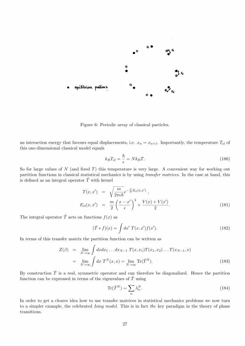
Figure 6: Periodic array of classical particles.

an interaction energy that favours equal displacements, i.e. xn = xn+1. Importantly, the temperature Tcl ofthis one-dimensional classical model equals

kBTcl =~ε

= NkBT. (180)

So for large values of N (and fixed T ) this temperature is very large. A convenient way for working outpartition functions in classical statistical mechanics is by using transfer matrices. In the case at hand, thisis defined as an integral operator T with kernel

T (x, x′) =

√m

2πε~e−

βNEcl(x,x

′) ,

Ecl(x, x′) =

m

2

(x− x′

ε

)2

+V (x) + V (x′)

2. (181)

The integral operator T acts on functions f(x) as

(T ∗ f)(x) =

∫dx′ T (x, x′)f(x′). (182)

In terms of this transfer matrix the partition function can be written as

Z(β) = limN→∞

∫dxdx1 . . . dxN−1 T (x, x1)T (x1, x2) . . . T (xN−1, x)

= limN→∞

∫dx TN (x, x) = lim

N→∞Tr(TN ). (183)

By construction T is a real, symmetric operator and can therefore be diagonalized. Hence the partitionfunction can be expressed in terms of the eigenvalues of T using

Tr(TN ) =∑n

λNn . (184)

In order to get a clearer idea how to use transfer matrices in statistical mechanics problems we now turnto a simpler example, the celebrated Ising model. This is in fact the key paradigm in the theory of phasetransitions.

27

5 The Ising Model

Ferromagnetism is an interesting phenomenon in solids. Some metals (like Fe or Ni) are observed to acquire afinite magnetization below a certain temperature. Ferromagnetism is a fundamentally quantum mechanicaleffect, and arises when electron spins spontaneously align along a certain direction. The Ising model is avery crude attempt to model this phenomenon. It is defined as follows. We have a lattice in D dimensionswith N sites. On each site j of this lattice sits a “spin” variable σj , which can take the two values ±1.These are referred to as “spin-up” and “spin-down” respectively. A given set {σ1, σ2, . . . , σN} specifies aconfiguration. The corresponding energy is taken to be of the form

E({σj}) = −J∑〈ij〉

σiσj − hN∑j=1

σj , (185)

where 〈ij〉 denote nearest-neighbour bonds on our lattice and J > 0. The first term favours alignmenton neighbouring spins, while h is like an applied magnetic field. Clearly, when h = 0 the lowest energystates are obtained by choosing all spins to be either up or down. The question of interest is whether theIsing model displays a finite temperature phase transition between a ferromagnetically ordered phase at lowtemperatures, and a paramagnetic phase at high temperatures.

5.1 Statistical mechanics of the Ising model

The partition function of the model is

Z =∑σ1=±1

∑σ2=±1

· · ·∑

σN=±1

e−βE({σj}). (186)

The magnetization per site is given by

m(h) =1

N〈N∑j=1

σj〉β =1

Nβ

∂

∂hln(Z). (187)

The magnetic susceptibility is defined as

χ(h) =∂m(h)

∂h=

1

Nβ

∂2

∂h2ln(Z). (188)

Substituting the expression (186) for the partition function and then carrying out the derivatives it can beexpressed in the form

χ(h) =β

N

N∑l,m=1

〈σlσm〉β − 〈σl〉β〈σm〉β. (189)

5.2 The One-Dimensional Ising Model

The simplest case is when our lattice is one-dimensional, and we impose periodic boundary conditions. Theenergy then reads

E =N∑j=1

[−Jσjσj+1 −

h

2(σj + σj+1)

]≡

N∑j=1

E(σj , σj+1), (190)

where we have definedσN+1 = σ1. (191)

The partition function can be expressed in the form

Z =∑

σ1,...,σN

N∏j=1

e−βE(σj ,σj+1). (192)

It can be evaluated exactly by means of the transfer matrix method.

28

5.2.1 Transfer matrix approach

The general idea is to rewrite Z as a product of matrices. The transfer matrix T is taken to be a 2 × 2matrix with elements

Tσσ′ = e−βE(σ,σ′). (193)

Its explicit form is

T =

(T++ T+−T−+ T−−

)=

(eβ(J+h) e−βJ

e−βJ eβ(J−h)

). (194)

The partition function can be expressed in terms of the transfer matrix as follows

Z =∑

σ1,...,σN

Tσ1σ2Tσ2σ3 . . . TσN−1σNTσNσ1 (195)

As desired, this has the structure of a matrix multiplication

Z = Tr(TN).

(196)

The trace arises because we have imposed periodic boundary conditions. As T is a real symmetric matrix,it can be diagonalized, i.e.

U †TU =

(λ+ 00 λ−

), (197)

where U is a unitary matrix and

λ± = eβJ cosh(βh)±√e2βJ sinh2(βh) + e−2βJ . (198)

Using the cyclicity of the trace and UU † = I, we have

Z = Tr(UU †TN

)= Tr

(U †TNU

)= Tr

([U †TU ]N

)= Tr

(λN+ 00 λN−

)= λN+ + λN− . (199)

But as λ− < λ+ we have

Z = λN+

(1 +

[λ−λ+

]N)= λN+

(1 + e−N ln(λ+/λ−)

). (200)

So for large N , which is the case we are interested in, we have with exponential accuracy

Z ' λN+ .(201)

Given the partition function, we can now easily calculate the magnetization per site

m(h) =1

Nβ

∂

∂hln(Z). (202)

In Fig. 7 we plot m(h) as a function of inverse temperature β = 1/kBT for two values of magnetic field h.We see that for non-zero h, the magnetization per site takes its maximum value m = 1 at low temperatures.At high temperatures it goes to zero. This is as expected, as at low T the spins align along the directionof the applied field. However, as we decrease the field, the temperature below which m(h) approaches unitydecreases. In the limit h→ 0, the magnetization per site vanishes at all finite temperatures. Hence there isno phase transition to a ferromagnetically ordered state in the one dimensional Ising model.

29

2 4 6 8 10

Β

0.2

0.4

0.6

0.8

1.0

mHh=0.1L

2 4 6 8 10

Β

0.2

0.4

0.6

0.8

1.0

mHh=10-5L

Figure 7: Magnetization per site as a function of inverse temperature for two values of applied magneticfield. We see that when we reduce the magnetic field, the temperature region in which the magnetization isessentially zero grows.

5.2.2 Averages of observables in the transfer matrix formalism

The average magnetization at site j is

〈σj〉β =1

Z

∑σ1,...,σN

σje−βE({σj}). (203)

We can express this in terms of the transfer matrix as

〈σj〉β =1

Z

∑σ1,...,σN

Tσ1σ2Tσ2σ3 . . . Tσj−1σjσjTσjσj+1 . . . TσNσ1 . (204)

Using that(Tσz)σj−1σj

= Tσj−1σjσj , (205)

where σz =

(1 00 −1

)is the Pauli matrix, we obtain

〈σj〉β =1

ZTr[T j−1σzTN−j+1

]=

1

ZTr[TNσz

]. (206)

Diagonalizing T by means of a unitary transformation as before, this becomes

〈σj〉β =1

ZTr[U †TNUU †σzU

]=

1

ZTr

[(λN+ 00 λN−

)U †σzU

]. (207)

The matrix U is given in terms of the normalized eigenvectors of T

T |±〉 = λ±|±〉 (208)

asU = (|+〉, |−〉). (209)

For h = 0 we have

U |h=0 =1√2

(1 11 −1

). (210)

This gives

〈σj〉β∣∣∣h=0

= 0. (211)

30

For general h the expression is more complicated

U =

α+√1+α2

+

α−√1+α2

−1√

1+α2+

1√1+α2

−

, α± =

√1 + e4βJ sinh2(βh)± e2βJ sinh(βh). (212)

The magnetization per site in the thermodynamic limit is then

limN→∞

〈σj〉β = limN→∞

(α2+−1

α2++1

)λN+ +

(α2−−1

α2−+1

)λN−

λN+ + λN−=

(α2

+ − 1

α2+ + 1

). (213)

This now allows us to prove, that in the one dimensional Ising model there is no phase transition at anyfinite temperature:

limh→0

limN→∞

〈σj〉β = 0 , β <∞.(214)

Note the order of the limits here: we first take the infinite volume limit at finite h, and only afterwardstake h to zero. This procedure allows for spontaneous symmetry breaking to occur, but the outcome of ourcalculation is that the spin reversal symmetry remains unbroken at any finite temperature.

Similarly, we find

〈σjσj+r〉β =1

ZTr[T j−1σzT rσzTN+1−j−r] =

1

ZTr

[U †σzU

(λr+ 00 λr−

)U †σzU

(λN−r+ 0

0 λN−r−

)]. (215)

We can evaluate this for zero field h = 0

〈σjσj+r〉β∣∣∣h=0

=λN−r+ λr− + λN−r− λr+

λN+ + λN−≈[λ−λ+

]r= e−r/ξ. (216)

So in zero field the two-point function decays exponentially with correlation length

ξ =1

ln coth(βJ). (217)

5.2.3 The related zero-dimensional quantum model

The 1D classical Ising model is related to a 0D quantum mechanical system as follows. Given the discussionleading to (181), we are looking to write the transfer matrix of the Ising model in the form

T =

√c

εe−εHQ/~, (218)

where c is a constant with dimension of time. Our transfer matrix can be written as

T = eβJ cosh(βh)I + eβJ sinh(βh)σz + e−βJσx (219)

We see that if we tune h to zero such that for large β

e−2βJ =εK

~, βhe2βJ = λ = fixed, (220)

then

T =

√~εK

(I +

εK

~[λσz + σx] +O(ε2)

). (221)

We conclude that the one dimensional classical Ising model is related to the quantum mechanics of a singlespin-1/2 with Hamiltonian

HQ = −Kσx −Kλσz. (222)

31

5.3 The Two-Dimensional Ising Model

We now turn to the 2D Ising model on a square lattice with periodic boundary conditions. The spin variableshave now two indices corresponding to rows and columns of the square lattice respectively

σj,k = ±1 , j, k = 1, . . . , N. (223)

The boundary conditions are σk,N+1 = σk,1 and σN+1,j = σ1,j , which correspond to the lattice “living” on

k,j

j

k

σ

Figure 8: Ising model on the square lattice.

the surface of a torus. The energy in zero field is

E({σk,j}) = −J∑j,k

σk,jσk,j+1 + σk,jσk+1,j . (224)

5.3.1 Transfer Matrix Method

The partition function is given by

Z =∑{σj,k}

e−βE({σk,j}). (225)

The idea of the transfer matrix method is again to write this in terms of matrix multiplications. Thedifference to the one dimensional case is that the transfer matrix will now be much larger. We start byexpressing the partition function in the form

Z =∑{σj,k}

e−β∑Nk=1 E(k;k+1), (226)

where

E(k; k + 1) = −JN∑j=1

σk,jσk+1,j +1

2[σk,jσk,j+1 + σk+1,jσk+1,j+1] . (227)

This energy depends only on the configurations of spins on rows k and k + 1, i.e. on spins σk,1, . . . , σk,Nand σk+1,1, . . . , σk+1,N . Each configuration of spins on a given row specifies a sequence s1, s2, . . . , sN withsj = ±1. Let us associate a vector

|s〉 (228)

with each such sequence. By construction there 2N such vectors. We then define a scalar product on thespace spanned by these vectors by

〈t|s〉 =N∏j=1

δtj ,sj . (229)

32

With this definition, the vectors {|s〉} form an orthonormal basis of a 2N dimensional linear vector space.In particular we have

I =∑s

|s〉〈s|. (230)

Finally, we define a 2N × 2N transfer matrix T by

〈σk|T |σk+1〉 = e−βE(k;k+1). (231)

The point of this construction is that the partition function can now be written in the form

Z =∑σ1

∑σ2

· · ·∑σN

〈σ1|T |σ2〉〈σ2|T |σ3〉 . . . 〈σN−1|T |σN 〉〈σN |T |σ1〉 (232)

We now may use (230) to carry out the sums over spins, which gives

Z = Tr[TN], (233)

where the trace is over our basis {|s〉|sj = ±1} of our 2N dimensional vector space. Like in the 1D case,thermodynamic properties involve only the largest eigenvalues of T . Indeed, we have

Z =

2N∑j=1

λNj , (234)

where λj are the eigenvalues of T . The free energy is then

F = −kBT ln(Z) = −kBT ln

λNmax

2N∑j=1

(λjλmax

)N = −kBTN ln(λmax)− kBT ln

∑j

(λjλmax

)N , (235)

where λmax is the largest eigenvalue of T , which we assume to be unique. As |λj/λmax| < 1, the secondcontribution in (235) is bounded by −kBTN ln(2), and we see that in the thermodynamic limit the freeenergy per site is

f = limN→∞

F

N2= lim

N→∞−kBT

Nln(λmax).

(236)

Thermodynamic quantities are obtained by taking derivatives of f and hence only involve the largest eigen-value of T . The main complication we have to deal with is that T is still a very large matrix. This posesthe question, why we should bother to use a transfer matrix description anyway? Calculating Z from itsbasic definition (225) involves a sum with 2N

2terms, i.e. at least 2N

2operations on a computer. Finding

the largest eigenvalue of a M ×M matrix involves O(M2) operations, which in our case amounts to O(22N ).For large values of N this amounts to an enormous simplification.

5.3.2 Spontaneous Symmetry Breaking

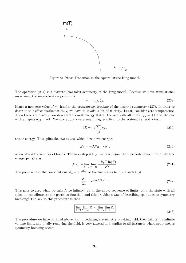
Surprisingly, the transfer matrix of the 2D Ising model can be diagonalized exactly. Unfortunately wedon’t have the time do go through the somewhat complicated procedure here, but the upshot is that the2D Ising model can be solved exactly. Perhaps the most important result is that in the thermodynamiclimit the square lattice Ising model has a finite temperature phase transition between a paramagnetic anda ferromagnetic phase. The magnetization per site behaves as shown in Fig.9. At low temperatures T < Tcthere is a non-zero magnetization per site, even though we did not apply a magnetic field. This is surprising,because our energy (224) is unchanged if we flip all spins

σj,k → −σj,k. (237)

33

1 T/T

m(T)

c

1

Figure 9: Phase Transition in the square lattice Ising model.

The operation (237) is a discrete (two-fold) symmetry of the Ising model. Because we have translationalinvariance, the magnetization per site is

m = 〈σj,k〉β. (238)

Hence a non-zero value of m signifies the spontaneous breaking of the discrete symmetry (237). In order todescribe this effect mathematically, we have to invoke a bit of trickery. Let us consider zero temperature.Then there are exactly two degenerate lowest energy states: the one with all spins σj,k = +1 and the onewith all spins σj,k = −1. We now apply a very small magnetic field to the system, i.e. add a term

δE = −ε∑j,k

σj,k (239)

to the energy. This splits the two states, which now have energies

E± = −JNB ∓ εN , (240)

where NB is the number of bonds. The next step is key: we now define the thermodynamic limit of the freeenergy per site as

f(T ) ≡ limε→0

limN→∞

−kBT ln(Z)

N2. (241)

The point is that the contributions Z± = e−βE± of the two states to Z are such that

Z−Z+

= e−2εN/kBT . (242)

This goes to zero when we take N to infinity! So in the above sequence of limits, only the state with allspins up contributes to the partition function, and this provides a way of describing spontaneous symmetrybreaking! The key to this procedure is that

limε→0

limN→∞

Z 6= limN→∞

limε→0

Z.

(243)

The procedure we have outlined above, i.e. introducing a symmetry breaking field, then taking the infinitevolume limit, and finally removing the field, is very general and applies to all instances where spontaneoussymmetry breaking occurs.

34

5.4 Homework Questions 8-10

Question 8. A lattice model for non-ideal gas is defined as follows. The sites i of a lattice may be empty oroccupied by at most one atom, and the variable ni takes the values ni = 0 and ni = 1 in the two cases. Thereis an attractive interaction energy J between atoms that occupy neighbouring sites, and a chemical potential µ.The model Hamiltonian is

H = −J∑〈ij〉

ninj − µ∑i

ni , (244)

where∑〈ij〉 is a sum over neighbouring pairs of sites.

(a) Describe briefly how the transfer matrix method may be used to calculate the statistical-mechanical propertiesof one-dimensional lattice models with short range interactions. Illustrate your answer by explaining how thepartition function for a one-dimensional version of the lattice gas, Eq. (1), defined on a lattice of N sites withperiodic boundary conditions, may be evaluated using the matrix

T =

(1 eβµ/2

eβµ/2 eβ(J+µ)

).

(b) Derive an expression for 〈ni〉 in the limit N →∞, in terms of elements of the eigenvectors of this matrix.(c) Show that

〈ni〉 =1

1 + e−2θ,

wheresinh(θ) = exp(βJ/2) sinh(β[J + µ]/2) .

Sketch 〈ni〉 as a function of µ for βJ � 1, and comment on the physical significance of your result.

Question 9. The one-dimensional 3-state Potts model is defined as follows. At lattice sites i = 0, 1, . . . , L“spin” variables σi take integer values σi = 1, 2, 3. The Hamiltonian is then given by

H = −JL−1∑i=0

δσi,σi+1 , (245)

where δa,b is the Kronecker delta, J > 0.(a) What are the ground states and first excited states for this model?(b) Write down the transfer matrix for (245). Derive an expression for the free energy per site f in the limitof large L in terms of the transfer matrix eigenvalues. Show that vectors of the form (1, z, z2) with z3 = 1 areeigenvectors, and hence find the corresponding eigenvalues. Show that at temperature T (with β = 1/kBT ) andin the limit L→∞

f = −kBT ln(

3 + eβJ − 1). (246)

(c) The boundary variable σ0 is fixed in the state σ0 = 1. Derive an expression (for large L), that the variableat site `� 1 is in the same state, in terms of the transfer matrix eigenvalues and eigenvectors. Show that yourresult has the form

〈δσ`,1〉 =1

3+

2

3e−`/ξ. (247)

How does ξ behave in the low and high temperature limits?

Question 10. Consider a one dimensional Ising model on an open chain with N sites, where N is odd. On alleven sites a magnetic field 2h is applied, see Fig. 10. The energy is

E = −JN−1∑j=1

σjσj+1 + 2h

(N−1)/2∑j=1

σ2j . (248)

35

2h

1 NJ J J J J J J J

2h 2h 2h

Figure 10: Open Ising chain with magnetic field applied to all even sites.

(a) Show that the partition function can be written in the form

Z = 〈u|T (N−1)/2|v〉 , (249)

where T is an appropriately constructed transfer matrix, and |u〉 and |v〉 two dimensional vectors. Give explicitexpressions for T , |u〉 and |v〉.(b) Calculate Z for the case h = 0.

36

Part III

Many-Particle Quantum Mechanics

In the basic QM course you encountered only quantum systems with very small numbers of particles. Inthe harmonic oscillator problem we are dealing with a single QM particle, when solving the hydrogen atomwe had one electron and one nucleus. Perhaps the most important field of application of quantum physicsis to systems of many particles. Examples are the electronic degrees of freedom in solids, superconductors,trapped ultra-cold atomic gases, magnets and so on. The methods you have encountered in the basic QMcourse are not suitable for studying such problems. In this part of the course we introduce a framework,that will allow us to study the QM of many-particle systems. This new way of looking at things will alsoreveal very interesting connections to Quantum Field Theory.

6 Second Quantization

The formalism we develop in the following is known as second quantization.

6.1 Systems of Independent Particles

You already know from second year QM how to solve problems involving independent particles

H =N∑j=1

Hj (250)

where Hj is the Hamiltonian on the j’th particle, e.g.

Hj =p2j

2m+ V (rj) = − ~2

2m∇2j + V (rj). (251)

The key to solving such problems is that [Hj , Hl] = 0. We’ll now briefly review the necessary steps,switching back and forth quite freely between using states and operators acting on them, and the positionrepresentation of the problem (i.e. looking at wave functions).

• Step 1. Solve the single-particle problem

Hj |φl〉 = El|φl〉 . (252)

The corresponding wave functions areφl(rj) = 〈rj |φl〉. (253)

The eigenstates form an orthonormal set

〈φl|φm〉 = δl,m =

∫dDrj φ

∗l (rj)φm(rj). (254)

• Step 2. Form N -particle eigenfunctions as products N∑j=1

Hj

φl1(r1)φl2(r2) . . . φlN (rN ) =

N∑j=1

Elj

φl1(r1)φl2(r2) . . . φlN (rN ) . (255)

This follows from the fact that in the position representation Hj is a differential operator that actsonly on the j’th position rj . The corresponding eigenstates are tensor products

|l1〉 ⊗ |l2〉 ⊗ · · · ⊗ |lN 〉. (256)

37

• Step 3. Impose the appropriate exchange symmetry for indistinguishable particles, e.g.

ψ±(r1, r2) =1√2

[φl(r1)φm(r2)± φl(r2)φm(r1)] , l 6= m. (257)

Generally we requireψ(. . . , ri, . . . , rj , . . . ) = ±ψ(. . . , rj , . . . , ri, . . . ) , (258)

where the + sign corresponds to bosons and the − sign to fermions. This is achieved by taking

ψl1...lN (r1, . . . , rN ) = N∑P∈SN

(±1)|P |φlP1 (r1) . . . φlPN (rN ),

(259)

where the sum is over all permutations of (1, 2, . . . , N) and |P | is the number of pair exchanges requiredto reduce (P1, . . . , PN ) to (1, . . . , N). The normalization constant N is

N =1√

N !n1!n2! . . ., (260)

where nj is the number of times j occurs in the set {l1, . . . , lN}. For fermions the wave functions canbe written as Slater determinants

ψl1...lN (r1, . . . , rN ) =1√N !

det

φl1(r1) . . . φl1(rN )...

...φlN (r1) . . . φlN (rN )

. (261)

The states corresponding to (259) are

|l1, . . . , lN 〉 = N∑P∈SN

(±1)|P ||lP1〉 ⊗ · · · ⊗ |lPN 〉 .

(262)

6.1.1 Occupation Number Representation

By construction the states have the symmetry

|lQ1 . . . lQN 〉 = ±|l1 . . . lN 〉 , (263)

where Q is an arbitrary permutation of (1, . . . , N). As the overall sign of state is irrelevant, we can thereforechoose them without loss of generality as

| 1 . . . 1︸ ︷︷ ︸n1

2 . . . 2︸ ︷︷ ︸n2

3 . . . 3︸ ︷︷ ︸n3

4 . . . 〉 ≡ |n1n2n3 . . . 〉. (264)

In (264) we have as many nj ’s as there are single-particle eigenstates, i.e. dimH 4. For fermions we havenj = 0, 1 only as a consequence of the Pauli principle. The representation (264) is called occupation numberrepresentation. The nj ’s tell us how many particles are in the single-particle state |j〉. By construction thestates {|n1n2n3 . . . 〉|

∑j nj = N} form an orthonormal basis of our N -particle problem

〈m1m2m3 . . . |n1n2n3 . . . 〉 =∏j

δnj ,mj , (265)

where we have defined 〈m1m2m3 . . . |=|m1m2m3 . . . 〉†.4Note that this is different from the particle number N .

38

6.2 Fock Space

We now want to allow the particle number to vary. The main reason for doing this is that we will encounterphysical problems where particle number is in fact not conserved. Another motivation is that experimentalprobes like photoemission change particle number, and we want to be able to describe these. The resultingspace of states is called Fock Space.

1. The state with no particles is called the vacuum state and is denoted by |0〉.

2. N -particle states are |n1n2n3 . . . 〉 with∑

j nj = N .

6.2.1 Creation and Annihilation Operators

Given a basis of our space of states we can define operators by specifying their action on all basis states.

• particle creation operators with quantum number l

c†l |n1n2 . . . 〉 =

{0 if nl = 1 for fermions√nl + 1(±1)

∑l−1j=1 nj |n1n2 . . . nl + 1 . . . 〉 else.

(266)

Here the + (−) sign applies to bosons (fermions).

• particle annihilation operators with quantum number l

cl|n1n2 . . . 〉 =√nl(±1)

∑l−1j=1 nj |n1n2 . . . nl − 1 . . . 〉 .

(267)

We note that (267) follows from (266) by

〈m1m2 . . . |c†l |n1n2 . . . 〉∗ = 〈n1n2 . . . |cl|m1m2 . . . 〉 . (268)

The creation and annihilation operators fulfil canonical (anti)commutation relations

[cl, cm] = 0 = [c†l , c†m] , [cl, c

†m] = δl,m bosons,

(269)

{cl, cm} = clcm + cmcl = 0 = {c†l , c†m} , {cl, c†m} = δl,m fermions.

(270)

ProofLet us see how to prove these in the fermionic case. For l < m we have

c†l cm| . . . nl . . . nm . . . 〉 = c†l√nm(−1)

∑m−1j=1 nj | . . . nl . . . nm − 1 . . . 〉

=√nl + 1

√nm(−1)

∑m−1j=l nj | . . . nl + 1 . . . nm − 1 . . . 〉. (271)

Similarly we have

cmc†l | . . . nl . . . nm . . . 〉 =

√nl + 1

√nm(−1)1+

∑m−1j=l nj | . . . nl + 1 . . . nm − 1 . . . 〉. (272)

This means that for any basis state |n1n2 . . . 〉 we have

{c†l , cm}|n1n2 . . . 〉 = 0 , if l > m. (273)

This implies that{c†l , cm} = 0 , if l > m. (274)

39

The case l < m works in the same way. This leaves us with the case l = m. Here we have

c†l cl| . . . nl . . . nm . . . 〉 = c†l√nl(−1)

∑l−1j=1 nj | . . . nl − 1 . . . 〉 = nl| . . . nl . . . 〉. (275)

clc†l | . . . nl . . . 〉 =

{cl√nl + 1(−1)

∑l−1j=1 nj | . . . nl + 1 . . . 〉 if nl = 0 ,

0 if nl = 1 ,

=

{| . . . nl . . . 〉 if nl = 0 ,

0 if nl = 1 ,(276)

Combining these we find that{c†l , cl}| . . . nl . . . 〉 = | . . . nl . . . 〉 , (277)

and as the states | . . . nl . . . 〉 form a basis this implies

{c†l , cl} = 1. (278)

Note that here 1 really means the identity operator 1.Proof

6.2.2 Basis of the Fock Space

We are now in a position to write down our Fock space basis in a very convenient way.

• Fock vacuum (state without any particles)|0〉. (279)

• Single-particle states|0 . . . 0 1︸︷︷︸

l

0 . . . 〉 = c†l |0〉 . (280)

• N -particle states

|n1n2 . . . 〉 =∏j

1√nj !

(c†j

)nj|0〉 . (281)

6.3 Homework Questions 11-13

Question 11. Consider a fermion ‘system’ with just one single-particle orbital, so that the only states of thesystem are |0〉 (unoccupied) and |1〉 (occupied). Show that we can represent the operators a and a† by thematrices

a† =

(0 0C 0

), a =

(0 C∗

0 0

).

You can do this by checking the values of aa, a†a† and a†a+ aa†. What values may the constant C take?

Question 12. A quantum-mechanical Hamiltonian for a system of an even number N of point unit massesinteracting by nearest-neighbour forces in one dimension is given by

H =1

2

N∑r=1

(p2r + (qr+1 − qr)2

),

40

where the Hermitian operators qr, pr satisfy the commutation relations [qr, qs] = [pr, ps] = 0, [qr, ps] = iδrs, andwhere qr+N = qr. New operators Qk, Pk are defined by

qr =1√N

∑k

Qkeikr and pr =

1√N

∑k

Pke−ikr,

where k = 2πn/N with n = −N/2 + 1, . . . , 0, . . . , N/2.

Show that:

(a) Qk =1√N

N∑s=1

qse−iks and Pk = 1√

N

∑Ns=1 pse

iks

(b) [Qk, Pk′ ] = iδkk′

(c) H = 12

(∑k PkP−k + ω2QkQ−k

), where ω2 = 2(1− cos k).

Similarly to the treatment of the simple harmonic oscillator in QM I we then define annihilation operators ak by

ak =1

(2ωk)1/2(ωkQk + iP−k).

Show that the Hermitian conjugate operators are

a†k =1

(2ωk)1/2(ωkQ−k − iPk),

and determine the canonical commutation relations for ak and a†p. Construct the Fock space of states and de-termine the eigenstates and eigenvalues of H.

Question 13. Bosonic creation operators are defined through their action on basis states in the occupationnumber representation as

c†l |n1n2 . . . 〉 =√nl + 1|n1n2 . . . nl + 1 . . . 〉 , (282)

a) Deduce from this how bosonic annihilation operators act.b) Show that the creation and annihilation operators fulfil canonical commutation relations

[cl, cm] = 0 = [c†l , c†m] , [cl, c

†m] = δl,m. (283)

6.3.1 Change of Basis

The Fock space is built from a given basis of single-particle states

single-particle states |l〉−→

N-particle states |n1n2 . . . 〉 −→Fock Space

. (284)

You know from second year QM that it is often convenient to switch from one basis to another, e.g. fromenergy to momentum eigenstates. This is achieved by a unitary transformation

{|l〉} −→ {|α〉} , (285)

where|α〉 =

∑l

〈l|α〉︸︷︷︸Ulα

|l〉. (286)

By construction ∑α

UlαU†αm =

∑α

〈l|α〉〈α|m〉 = 〈l|m〉 = δlm. (287)

41

We now want to “lift” this unitary transformation to the level of the Fock space. We know that

|l〉 = c†l |0〉 ,|α〉 = d†α|0〉 . (288)

On the other hand we have|α〉 =

∑l

Ulα|l〉 =∑l

Ulαc†l |0〉. (289)

This suggests that we take

d†α =∑l

Ulαc†l ,

(290)

and this indeed reproduces the correct transformation for N -particle states. Taking the hermitian conjugatewe obtain the transformation law for annihilation operators

dα =∑l

U †αlcl.

(291)

We emphasize that these transformation properties are compatible with the (anti)commutation relations (asthey must be). For fermions

{dα, d†β} =∑l,m

U †αlUmβ {cl, c†m}︸ ︷︷ ︸

δl,m

=∑l

U †αlUlβ = (U †U)αβ = δα,β. (292)

6.4 Second Quantized Form of Operators

In the next step we want to know how observables such as H, P , X etc act on the Fock space.

6.4.1 Occupation number operators

These are the simplest hermitian operators we can build from cl and c†m. They are defined as

nl ≡ c†l cl. (293)

From the definition of cl and c†l it follows immediately that

nl|n1n2 . . . 〉 = nl|n1n2 . . . 〉. (294)

6.4.2 Single-particle operators

Single-particle operators are of the form

O =∑j

oj , (295)

where the operator oj acts only on the j’th particle. Examples are kinetic and potential energy operators

T =∑j

p2j

2m, V =

∑j

V (xj). (296)

We want to represent O on the Fock space built from single-particle eigenstates |α〉. We do this in two steps:

42

• Step 1: We first represent O on the Fock space built from the eigenstates of o

o|l〉 = λl|l〉 = λlc†l |0〉. (297)

Then, when acting on an N -particle state (262), we have

O|l1, l2, . . . , lN 〉 =

N∑j=1

λj

|l1, l2, . . . , lN 〉. (298)

This is readily translated into the occupation number representation

O|n1n2 . . . 〉 =

[∑k

nkλk

]|n1n2 . . .〉. (299)

As |n1n2 . . . 〉 constitute a basis, this together with (294) imply that we can represent O in the form

O =∑k

λknk =∑k

λkc†kck. (300)

• Step 2: Now that we have a representation of O on the Fock space built from the single-particle states|l〉, we can use a basis transformation to the basis {|α〉} to obtain a representation on a general Fockspace. Using that 〈k|O|k′〉 = δk,k′λk we can rewrite (300) in the form

O =∑k,k′

〈k′|O|k〉c†k′ck. (301)

Then we apply our general rules for a change of single-particle basis of the Fock space

c†k =∑α

U †αkd†α. (302)

This gives

O =∑α,β

∑k′

(〈k′|U †αk′

)︸ ︷︷ ︸

〈α|

O∑k

(Ukβ|k〉

)︸ ︷︷ ︸

|β〉

d†αdβ. (303)

where we have used that|k〉 =

∑α

U †αk|α〉 . (304)

This gives us the final result

O =∑α,β

〈α|O|β〉 d†αdβ.

(305)

We now work out a number of explicit examples of Fock space representations for single-particle operators.

1. Momentum Operators P in the infinite volume:

(i) Let us first consider P in the single-particle basis of momentum eigenstates

P|k〉 = k|k〉 , 〈p|k〉 = (2π~)3δ(3)(p− k). (306)

Remark

43

These are shorthand notations for

Pa|kx, ky, kz〉 = ka|kx, ky, kz〉 , a = x, y, z. (307)

and〈px, py, pz|kx, ky, kz〉 = (2π~)3δ(kx − px)δ(ky − py)δ(kz − pz) . (308)

RemarkUsing our general result for representing single-particle operators in a Fock space built from theireigenstates (300) we have

P =

∫d3p

(2π~)3pc†(p)c(p) , [c†(k), c(p)} = (2π~)3δ(3)(p− k). (309)

Here we have introduced a notation

[c†(k), c(p)} =

{c†(k)c(p)− c(p)c†(k) for bosons

c†(k)c(p) + c(p)c†(k) for fermions.(310)

(ii) Next we want to represent P in the single-particle basis of position eigenstates

X|x〉 = x|x〉 , 〈x|x′〉 = δ(3)(x− x′). (311)

Our general formula (305) gives

P =

∫d3xd3x′ 〈x′|P|x〉c†(x′)c(x) . (312)

We can simplify this by noting that

〈x′|P|x〉 = −i~∇x′δ(3)(x− x′), (313)

which allows us to eliminate three of the integrals

P =

∫d3xd3x′

[−i~∇x′δ

(3)(x− x′)]c†(x′)c(x) =

∫d3xc†(x) (−i~∇x) c(x). (314)

2. Single-particle Hamiltonian:

H =N∑j=1

p2j

2m+ V (xj). (315)

(i) Let us first consider H in the single-particle basis of energy eigenstates H|l〉 = El|l〉, |l〉 = c†l |0〉.Our result (300) tells us that

H =∑l

Elc†l cl. (316)

(ii) Next we consider the position representation, i.e. we take position eigenstates |x〉 = c†(x)|0〉 as abasis of single-particle states. Then by (305)

H =

∫d3xd3x′ 〈x′|H|x〉 c†(x′)c(x). (317)

Substituting (315) into (317) and using

〈x′|V (x)|x〉 = V (x)δ(3)(x− x′) , 〈x′|p2|x〉 = −~2∇2δ(3)(x− x′) , (318)

44

we arrive at the position representation

H =

∫d3x c†(x)

[−~2∇2

2m+ V (x)

]c(x).

(319)

(iii) Finally we consider the momentum representation, i.e. we take momentum eigenstates |p〉 =c†(p)|0〉 as a basis of single-particle states. Then by (305)

H =

∫d3pd3p′

(2π~)6〈p′|H|p〉 c†(p′)c(p). (320)

Matrix elements of the kinetic energy operator are simple

〈p′|p2|p〉 = p2〈p′|p〉 = p2(2π~)3δ(3)(p− p′). (321)

Matrix elements of the potential can be calcuated as follows

〈p′|V |p〉 =

∫d3xd3x′ 〈p′|x′〉〈x′|V |x〉〈x|p〉 =

∫d3xd3x′ 〈x′|V |x〉︸ ︷︷ ︸

V (x)δ(3)(x−x′)

ei~p·x−

i~p′·x′

=

∫d3x V (x)e

i~ (p−p′)·x = V (p− p′), (322)

where V (p) is essentially the three-dimensional Fourier transform of the (ordinary) function V (x).Hence

H =

∫d3p

(2π~)3

p2

2mc†(p)c(p) +

∫d3pd3p′

(2π~)6V (p− p′)c†(p′)c(p).

(323)

6.4.3 Two-particle operators

These are operators that act on two particles at a time. A good example is the interaction potential V (r1, r2)between two particles at positions r1 and r2. For N particles we want to consider

V =N∑i<j

V (ri, rj). (324)

On the Fock space built from single-particle position eigenstates this is represented as

V =1

2

∫d3rd3r′ c†(r)c†(r′)V (r, r′)c(r′)c(r).

(325)

Note that when writing down the first quantized expression (324), we assumed that the operators actsspecifically on states with N particles. On the other hand, (325) acts on the Fock space, i.e. on stateswhere the particle number can take any value. The action of (325) on N -particle states (where N is fixedbut arbitrary) is equal to the action of (324).

Derivation of (325)Let us concentrate on the fermionic case. The bosonic case can be dealt with analogously. We start with ouroriginal representation of N -particle states (262)

|r1, . . . , rN 〉 = N∑P∈SN

(−1)|P ||r1〉 ⊗ . . . |rN 〉 . (326)

45

Then

V |r1, . . . , rN 〉 =∑i<j

V (ri, rj)|r1, . . . , rN 〉 =1

2

∑i 6=j

V (ri, rj)|r1, . . . , rN 〉 . (327)

On the other hand we know that

|r1, . . . , rN 〉 =

N∏j=1

c†(rj)|0〉. (328)

Now consider

c(r)|r1, . . . , rN 〉 = c(r)

N∏j=1

c†(rj)|0〉 = [c(r),

N∏j=1

c†(rj)}|0〉 , (329)

where is the last step we have used that c(r)|0〉 = 0, and [A,B} is an anticommutator ifboth A and B involve an odd number of fermions and a commutator otherwise.In our case we have a commutator for even N and an anticommutator for odd N .By repeatedly adding and subtracting terms we find that

[c(r),N∏j=1

c†(rj)} = {c(r), c†(r1)}N∏j=2

c†(rj)− c†(r1){c(r), c†(r2)}N∏j=3

c†(rj)

+ . . .+N−1∏j=1

c†(rj){c(r), c†(rN )}. (330)

Using that {c(r), c†(rj)} = δ(3)(r− rj) we then find

c(r)|r1, . . . , rN 〉 =

N∑n=1

(−1)n−1δ(3)(r− rn)

N∏j 6=n

c†(rj)|0〉 =

N∑n=1

(−1)n−1δ(3)(r− rn)|r1 . . .

missing︷︸︸︷rn . . . rN 〉. (331)

Hence

c†(r′)c(r′)︸ ︷︷ ︸number op.

c(r)|r1, . . . , rN 〉 =N∑n=1

(−1)n−1δ(3)(r− rn)N∑

m 6=nδ(3)(r′ − rm) |r1 . . .

missing︷︸︸︷rn . . . rN 〉, (332)

and finally

c†(r)c†(r′)c(r′)c(r)|r1, . . . , rN 〉 =N∑n=1

δ(3)(r− rn)N∑

m6=nδ(3)(r′ − rm) |r1 . . . rn . . . rN 〉. (333)

This implies that

1

2

∫d3rd3r′ V (r, r′) c†(r)c†(r′)c(r′)c(r)|r1, . . . , rN 〉 =

1

2

∑n6=m

V (rn, rm)|r1, . . . , rN 〉. (334)

As {|r1, . . . , rN 〉} form a basis, this establishes (325).Derivation of (325)

Using our formula for basis transformations (290)

c†(r) =∑l

〈l|r〉 c†l , (335)

we can transform (325) into a general basis. We have

V =1

2

∑ll′mm′

∫d3rd3r′ V (r, r′)〈l|r〉〈l′|r′〉〈r′|m′〉〈r|m〉c†l c

†l′cm′cm . (336)

46

We can rewrite this by using that the action of V on two-particle states is obtained by taking N = 2 in(324), which tells us that V |r〉 ⊗ |r′〉 = V (r, r′)|r〉 ⊗ |r′〉. This implies

V (r, r′)〈l|r〉〈l′|r′〉〈r′|m′〉〈r|m〉 = V (r, r′)[〈l| ⊗ 〈l′|

] [|r〉 ⊗ |r′〉|

] [〈r| ⊗ 〈r′|

] [|m〉 ⊗ |m′〉|

]=

[〈l| ⊗ 〈l′|

]V[|r〉 ⊗ |r′〉|

] [〈r| ⊗ 〈r′|

] [|m〉 ⊗ |m′〉|

](337)

Now we use that ∫d3rd3r′

[|r〉 ⊗ |r′〉

] [〈r| ⊗ 〈r′|

]= 1 (338)

to obtain

V =1

2

∑l,l′,m,m′

[〈l| ⊗ 〈l′

]|V |[m〉 ⊗ |m′〉

]c†l c†l′cm′cm. (339)

Finally we can express everything in terms of states with the correct exchange symmetry

|mm′〉 =1√2

[|m〉 ⊗ |m′〉 ± |m′〉 ⊗ |m〉

](m 6= m′). (340)

in the form

V =∑

(ll′),(mm′)

〈ll′|V |mm′〉c†l c†l′cm′cm .

(341)

Here the sums are over a basis of 2-particle states. In order to see that (339) is equal to (341) observe that∑m,m′

[|m〉 ⊗ |m′〉]cm′cm =1

2

∑m,m′

[|m〉 ⊗ |m′〉 ± |m′〉 ⊗ |m〉]cm′cm =1√2

∑m,m′

|mm′〉 cm′cm (342)

Here the first equality follows from relabelling summation indices m↔ m′ and using the (anti)commutationrelations between cm and cm′ to bring them back in the right order. The second equality follows from thedefinition of 2-particle states |mm′〉. Finally we note that because |mm′〉 = ±|m′m〉 (the minus sign is forfermions) we have

1√2

∑m,m′

|mm′〉 cm′cm =√

2∑

(mm′)

|mm′〉 cm′cm, (343)

where the sum is now over a basis of 2-particle states with the appropriate exchange symmetry. Therepresentation (341) generalizes to arbitrary two-particle operators O.

6.5 Homework Question 14

Question 14. Consider the N -particle interaction potential

V =

N∑i<j

V (ri, rj),

where V (ri, rj) = V (rj , ri). Show that in second quantization it is expressed as

V =1

2

∫d3rd3r′ V (r, r′) c†(r)c†(r′)c(r′)c(r).

To do so consider the action of V on a basis of N -particle position eigenstates

|r1 . . . rN 〉 =1√

N !n1!n2! . . .

∑P

(±1)|P ||r1〉 ⊗ |r2〉 ⊗ |rN 〉 =1√

n1!n2! . . .

N∏j=1

c†(rj)|0〉 ,

47

where nj is the occupation number of the jth single-particle state. Argue that in an arbitrary basis of single-particleeigenstates |l〉 V can be expressed in the form

V =∑ll′mm′

〈ll′|V |mm′〉c†l c†l′cm′cm.

7 Application I: The Ideal Fermi Gas

Consider an ideal gas of spin-1/2 fermions. The creation operators in the momentum representation (in theinfinite volume) are

c†σ(p) , σ =↑, ↓ . (344)

They fulfil canonical anticommutation relations

{cσ(p), cτ (k)} = 0 = {c†σ(p), c†τ (k)} , {cσ(p), c†τ (k)} = δσ,τ (2π~)3δ(3)(k− p). (345)

The Hamiltonian, in the grand canonical ensemble, is

H − µN =

∫d3p

(2π~)3

[p2

2m− µ

]︸ ︷︷ ︸

ε(p)

∑σ=↑,↓

c†σ(p)cσ(p). (346)

Here µ > 0 is the chemical potential. As c†σ(p)cσ(p) = nσ(p) is the number operator for spin-σ fermionswith momentum p, we can easily deduce the action of the Hamiltonian on states in the Fock space:[

H − µN]|0〉 = 0 ,[

H − µN]c†σ(p)|0〉 = ε(p) c†σ(p)|0〉 ,[

H − µN] n∏j=1

c†σj (pj)|0〉 =

[n∑k=1

ε(pk)

]n∏j=1

c†σj (pj)|0〉 . (347)

7.1 Quantization in a large, finite volume

In order to construct the ground state and low-lying excitations, it is convenient to work with a discrete setof momenta. This is achieved by considering the gas in a large, periodic box of linear size L. Momentumeigenstates are obtained by solving the eigenvalue equation e.g. in the position representation

pψk(r) = −i~∇ψk(r) = kψk(r). (348)

The solutions are plane waves

ψk(r) = ei~k·r. (349)

Imposing periodic boundary conditions (ea is the unit vector in a direction)

ψk(r + Lea) = ψk(r) for a = x, y, z, (350)

gives quantization conditions for the momenta k

ei~Lka = 1⇒ ka =

2π~naL

, a = x, y, z. (351)

To summarize, in a large, periodic box the momenta are quantized as

k =2π~L

nxnynz

(352)

48

Importantly, we can now normalize the eigenstates to 1, i.e.

ψk(r) =1

L32

ei~k·r. (353)

Hence

〈k|k′〉 =

∫d3rψ∗k(r)ψk′(r) = δk,k′ . (354)

As a consequence of the different normalization of single-particle states, the anticommutation relations ofcreation/annihilation operators are changed and now read

{cσ(p), cτ (k)} = 0 = {c†σ(p), c†τ (k)} , {c†σ(p), cτ (k)} = δσ,τδk,p. (355)

The Hamiltonian is

H − µN =∑p

ε(p)∑σ=↑,↓

c†σ(p)cσ(p).

(356)

We define a Fermi momentum byp2F

2m= µ. (357)

7.1.1 Ground State

Then the lowest energy state is obtained by filling all negative energy single-particle states, i.e.

|GS〉 =∏

|p|<pF ,σ

c†σ(p)|0〉.

(358)

The ground state energy is

EGS =∑σ

∑|p|<pF

ε(p). (359)

This is extensive (proportional to the volume) as expected. You can see the advantage of working in a finitevolume: the product in (358) involves only a finite number of factors and the ground state energy is finite.The ground state momentum is

PGS =∑σ

∑|p|<pF

p = 0. (360)

The ground state momentum is zero, because is a state with momentum p contributes to the sum, then sodoes the state with momentum −p.

(p)

p

ε

Figure 11: Ground state in the 1 dimensional case. Blue circles correspond to “filled” single-particle states.

49

7.1.2 Excitations

• Particle excitationsc†σ(k)|GS〉 with |k| > pF . (361)

Their energies and momenta are

E = EGS + ε(k) > EGS , P = k. (362)

• Hole excitationscσ(k)|GS〉 with |k| < pF . (363)

Their energies and momenta are

E = EGS − ε(k) > EGS , P = −k. (364)

• Particle-hole excitationsc†σ(k)cτ (p)|GS〉 with |k| > pF > |p|. (365)

Their energies and momenta are

E = EGS + ε(k)− ε(p) > EGS , P = k− p. (366)

(p)

p

ε (p)

p

ε (p)

p

ε

Figure 12: Some simple excited states: (a) particle (b) hole (c) particle-hole.

7.1.3 Density Correlations

Consider the single-particle operatoro = |r〉〈r| (367)

It represents the particle density at position |r〉 as can be seen by acting on position eigenstates. In secondquantization it is

ρ(r) =∑σ

∫d3r′d3r′′ 〈r′|o|r′′〉 c†σ(r′)cσ(r′′) =

∑σ

c†σ(r)cσ(r). (368)

1. One-point function.

We now want to determine the expectation value of this operator in the ground state

〈GS|ρ(r)|GS〉 =∑σ

〈GS|c†σ(r)cσ(r)|GS〉. (369)

50

A crucial observation is that the ground state has a simple description in terms of the Fock space builtfrom momentum eigenstates. Hence what we want to do is to work out the momentum representationof ρ(r). We know from our general formula (291) that

cσ(r) =∑p

〈r|p〉︸ ︷︷ ︸L−3/2e

i~p·r

cσ(p). (370)

Substituting this as well as the analogous expression for the creation operator into (369), we obtain

〈GS|ρ(r)|GS〉 =∑σ

1

L3

∑p,p′

ei~ (p−p′)·r〈GS|c†σ(p′)cσ(p)|GS〉. (371)

For the expectation value 〈GS|c†σ(p′)cσ(p)|GS〉 to be non-zero, we must have that c†σ(p′)cσ(p)|GS〉reproduces |GS〉 itself. The only way this is possible is if |p| < pF (so that the c pokes a hole in theFermi sea) and p′ = p (so that the c† precisely fills the hole made by the c). By this reasoning wehave

〈GS|c†σ(p′)cτ (p)|GS〉 = δσ,τδp,p′θ(pF − |p′|). (372)

Similarly we can show that

〈GS|cσ(p′)c†τ (p)|GS〉 = δσ,τδp,p′θ(|p| − pF ),

〈GS|cσ(p′)cτ (p)|GS〉 = 0 = 〈GS|c†σ(p′)c†τ (p)|GS〉. (373)

Substituting (372) back into (371) we find

〈GS|ρ(r)|GS〉 =∑σ

1

L3

∑p,p′

ei~ (p−p′)·rδp,p′ θ(pF − |p|) = 2︸︷︷︸

spin

1

L3

∑p

θ(pF − |p|) =N

L. (374)

So our expectation value gives precisely the particle density. This is expected because our system istranslationally invariant and therefore 〈GS|ρ(r)|GS〉 cannot depend on r.

2. Two-point function.

Next we want to determine the two-point function

〈GS|ρ(r)ρ(r′)|GS〉 =∑σ,τ

1

L6

∑p,p′

∑k,k′

ei~ (p−p′)·re

i~ (k−k′)·r′〈GS|c†σ(p′)cσ(p)c†τ (k′)cτ (k)|GS〉. (375)

The expectation value 〈GS|c†σ(p′)cσ(p)c†τ (k′)cτ (k)|GS〉 can be calculated by thinking about how thecreation and annihilation operators act on the ground state, and then concentrating on the processesthat reproduce the ground state itself in the end (see Fig. 13).

The result is

〈GS|c†σ(p′)cσ(p)c†τ (k′)cτ (k)|GS〉 = δk,k′δp,p′θ(pF − |p|)θ(pF − |k|)+δσ,τδp,k′δk,p′θ(|k′| − pF )θ(pF − |k|). (376)

Observe that by virtue of (372) and (373) this can be rewritten in the form

〈GS|c†σ(p′)cσ(p)|GS〉〈GS|c†τ (k′)cτ (k)|GS〉+ 〈GS|c†σ(p′)cτ (k)|GS〉〈GS|cσ(p)c†τ (k′)|GS〉 . (377)

The fact that the 4-point function (376) can be written as a sum over products of two-point functions is areflection of Wick’s theorem for noninteracting spin-1/2 fermions. This is not part of the syllabus and we

51

Figure 13:

won’t dwell on it, but apart from extra minus signs, this says that 2n-point functions are given by the sumover all possible “pairings”, giving rise to a product of two-point functions. In our particular case this gives

〈c†σ(p′)cσ(p)c†τ (k′)cτ (k)〉 = 〈c†σ(p′)cσ(p)〉〈c†τ (k′)cτ (k)〉 − 〈c†σ(p′)c†τ (k′)〉〈cσ(p)cτ (k)〉+ 〈c†σ(p′)cτ (k)〉〈cσ(p)c†τ (k′)〉, (378)

and using that the two point function of two creation or two annihilation operators is zero we obtain (377).Substituting (376) back in to (375) gives

〈GS|ρ(r)ρ(r′)|GS〉 =∑σ,σ′

1

L6

∑k,p

θ(pF − |k|)θ(pF − |p|)

+∑σ

1

L6

∑k,k′

θ(|k| − pF )θ(pF − |k′|)ei~ (k−k′)·(r−r′)

= 〈GS|ρ(r)|GS〉〈GS|ρ(r′)|GS〉+ 21

L3

∑|k|>pF

ei~k·(r−r

′) 1

L3

∑|k′|<pF

e−i~k′·(r−r′). (379)

RemarkEvaluting the k sums for large L: The idea is to turn sums into integrals

1

L3

∑|k|<pF

ei~k·R −→

∫d3k

(2π~)3θ(pF − |k|)e

i~k·R =

∫ ∞0

dpp2

∫ π

0dϑ sinϑ

∫ 2π

0dϕ

θ(pF − ~p)(2π)3

eip|R| cosϑ

=

∫ pF /~

0

dp

(2π)2

2p sin(p|R|)|R|

=sin(pF |R|)− pF |R| cos(pF |R|)

2π2|R|3≡ h(|R|). (380)

52

Here we have introduced spherical polar coordinates such that the z-axis of our co-ordinate system is along theR direction, and

kx = ~p sinϑ cosϕ ,

ky = ~p sinϑ sinϕ ,

kz = ~p cosϑ. (381)

The other sum works similarly

1

L3

∑|k|>pF

ei~k·R =

1

L3

∑k

ei~k·R − 1

L3

∑|k|<pF

ei~k·R. (382)

The second part is evaluated above, while the first part is

1

L3

∑k

ei~k·R = δ(3)(R). (383)

The equality can be proved by multiplying both sides by a test-function f(R)and then integrating over R:∫

d3R1

L3

∑k

ei~k·Rf(R) =

1

L3

∑k

∫d3Re

i~k·Rf(R) =

1

L3

∑k

fk = f(0). (384)

Here we have used standard definitions for Fourier series, cf Riley/Hobson/Bence 12.7.Remark

Using these simplifications for large L we arrive at our final answer

〈GS|ρ(r)ρ(r′)|GS〉 = 〈GS|ρ(r)|GS〉2 + 〈GS|ρ(r)|GS〉δ(3)(r− r′)− 2[h(|r− r′|)

]2.

(385)

The first two terms are the same as for a classical ideal gas, while the third contribution is due to thefermionic statistics (Pauli exclusion: “fermions don’t like to be close to one another”).

7.2 Homework Questions 15-16

Question 15. Consider a system of fermions moving freely on a one-dimensional ring of length L, i.e. periodicboundary conditions are applied between x = 0 and x = L. The fermions are all in the same spin state, so thatspin quantum numbers may be omitted. Fermion creation and annihilation operators at the point x are denotedby ψ†(x) and ψ(x).a) Write down the complete set of anticommutation relation satisfied by ψ†(x1) and ψ(x2).b) Write down the wave-functions of single-particle momentum eigenstates (make sure to take the boundaryconditions into account!). What are the allowed values of momentum? Using this result, derive an expression for

the momentum space creation and annihilation operators Ψ†p and Ψp in terms of ψ†(x) and ψ(x) (hint: use thegeneral result for basis transformation obtained in the lecture notes).

c) Starting with your expression for the anticommutator {ψ†(x1), ψ(x2)}, evaluate {Ψ†p,Ψq}.d) Derive an expression for ψ(x) in terms of Ψk.e) The density operator ρ(x) is defined by ρ(x) = ψ†(x)ψ(x). The number operator is

N =

∫ L

0dx ρ(x) .

Express ρ(x) in terms of Ψ†p and Ψq, and show from this that

N =∑k

Ψ†kΨk .

53

Let |0〉 be the vacuum state (containing no particles) and define |φ〉 by

|φ〉 = A∏k

(uk + vkΨ†k)|0〉,

where uk and vk are complex numbers depending on the label k, and A is a normalisation constant.Evaluate (i) |A|2, (ii) 〈φ|N |φ〉, and (iii) 〈φ|N2|φ〉. Under what conditions is |φ〉 an eigenstate of particle

number?

Question 16. Consider a system of fermions in which the functions ϕ`(x), ` = 1, 2 . . . N , form a completeorthonormal basis for single particle wavefunctions.a) Explain how Slater determinants may be used to construct a complete orthonormal basis for n-particle stateswith n = 2, 3 . . . N . Calculate the normalisation constant for such a Slater determinant at a general value of n.How many independent n-particle states are there for each n?b) Let C†` and C` be fermion creation and destruction operators which satisfy the usual anticommutation relations.The quantities ak are defined by

ak =N∑`=1

Uk`C`,

where Uk` are elements of an N × N matrix, U . Write down an expression for a†k. Find the condition which

must be satisfied by the matrix U in order that the operators a†k and ak also satisfy fermion anticommutationrelations.c) Non-interacting spinless fermions move in one dimension in an infinite square-well potential, with positioncoordinate 0 ≤ x ≤ L. The normalised single particle energy eigenstates are

ϕ`(x) =

(2

L

)1/2

sin

(`πx

L

),

and the corresponding fermion creation operator is C†` .Write down expressions for C†(x), the fermion creation operator at the point x, and for ρ(x), the particle

density operator, in terms of C†` , C` and ϕ`(x).d) What is the ground state expectation value 〈ρ(x)〉 in a system of n fermions?

In the limit n→∞, L→∞, taken at fixed average density ρ0 = n/L, show that

〈ρ(x)〉 = ρ0

[1− sin 2πρ0x

2πρ0x

].

Sketch this function and comment briefly on its behaviour for x→ 0 and x→∞.

8 Application II: Weakly Interacting Bosons

As you know from Statistical Mechanics, the ideal Bose gas displays the very interesting phenomenon ofBose condensation. This has been observed in systems of trapped Rb atoms and led to the award of theNobel prize in 2001 to Ketterle, Cornell and Wiemann. The atoms in these experiments are bosonic, but theatom-atom interactions are not zero. We now want to understand the effects of interactions in the frameworkof a microscopic theory. The kinetic energy operator is expressed in terms of creation/annihilation operatorssingle-particle momentum eigenstates as

T =∑p

p2

2mc†(p)c(p). (386)

54

Here we have assumed that our system in enclosed in a large, periodic box of linear dimension L. Theboson-boson interaction is most easily expressed in position space

V =1

2

∫d3rd3r′ c†(r)c†(r′)V (r, r′)c(r′)c(r) (387)

A good model for the potential V (r, r′) is to take it of the form

V (r, r′) = Uδ(3)(r− r′), (388)

i.e. bosons interact only if they occupy the same point in space. Changing to the momentum spacedescription

c(r) =1

L3/2

∑p

ei~p·rc(p), (389)

we have

V =U

2L3

∑p1,p2,p3

c†(p1)c†(p2)c(p3)c(p1 + p2 − p3). (390)

8.1 Ideal Bose Gas

For U = 0 we are dealing with an ideal Bose gas and we know that the ground state is a condensate: allparticles occupy the lowest-energy single-particle state, i.e. the zero-momentum state

|GS〉0 =1√N !

(c†(p = 0)

)N|0〉. (391)

So p = 0 is special, and in particular we have

0〈GS|c†(p = 0)c(p = 0)|GS〉0 = N. (392)

8.2 Bogoliubov Approximation

For small U > 0 we expect the Bose-Einstein condensate to persist, i.e. we expect

〈GS|c†(p = 0)c(p = 0)|GS〉 = N0 � 1. (393)

However,[c†(0)c(0), V ] 6= 0, (394)

so that the number of p = 0 bosons is not conserved, and the ground state |GS〉 will be a superposition ofstates with different numbers of p = 0 bosons. However, for the ground state and low-lying excited stateswe will have

〈Ψ|c†(0)c(0)|Ψ〉 ' N0 , (395)

where N0, crucially, is a very large number. The Bogoliubov approximation states that, when acting on theground state or low-lying excited states, we in fact have

c†(0) '√N0 , c(0) '

√N0 ,

(396)

i.e. creation and annihilation operators are approximately diagonal. This is a much stronger statement than(395), and at first sight looks rather strange. It amounts to making an ansatz for low-energy states |ψ〉 thatfulfils

〈ψ′|c(0)|ψ〉 =√N0〈ψ′|ψ〉+ . . . (397)

55

where the dots denote terms that are small compared to√N0. We’ll return to what this implies for the

structure of |ψ〉 a little later. Using (396) we may expand H in inverse powers of N0

H =∑p

p2

2mc†(p)c(p)

+U

2L3N2

0 +UN0

2L3

∑k 6=0

2c†(k)c(k) + 2c†(−k)c(−k) + c†(k)c†(−k) + c(−k)c(k)

+ . . . (398)

Now use thatN0 = c†(0)c(0) = N −

∑p6=0

c†(p)c(p), (399)

where N is the (conserved) total number of bosons, and define

ρ =N

L3= density of particles. (400)

Then our Hamiltonian becomes

H =Uρ

2N +

∑p6=0

[p2

2m+ Uρ

]︸ ︷︷ ︸

ε(p)

c†(p)c(p) +Uρ

2

[c†(p)c†(−p) + c(−p)c(p)

]+ . . .

(401)

The Bogoliubov approximation has reduced the complicated four-boson interaction to two-boson terms. Theprice we pay is that we have to deal with the “pairing”-terms quadratic in creation/annihilation operators.

8.3 Bogoliubov Transformation

Consider the creation/annihilation operators defined by(b(p)b†(−p)

)=

(cosh(θp) sinh(θp)sinh(θp) cosh(θp)

)(c(p)

c†(−p).

)(402)

It is easily checked that for any choice of Bogoliubov angle θp

[b(p), b(q)] = 0 = [b†(p), b†(q)] , [b(p), b†(q)] = δp,q. (403)

In terms of the Bogoliubov bosons the Hamiltonian becomes

H = const +1

2

∑p6=0

[(p2

2m+ Uρ

)cosh(2θp)− Uρ sinh(2θp)

] [b†(p)b(p) + b†(−p)b(−p)

]−[(

p2

2m+ Uρ

)sinh(2θp)− Uρ cosh(2θp)

] [b†(p)b†(−p) + b(−p)b(p)

]+ . . . (404)

Now we choose

tanh(2θp) =Uρ

p2

2m + Uρ, (405)

as this removes the b†b† + bb terms, and leaves us with a diagonal Hamiltonian

H = const +∑p6=0

E(p)b†(p)b(p) + . . .

(406)

56

where

E(p) =

√(p2

2m+ Uρ

)2

− (Uρ)2 . (407)

We note that

E(p) −→ p2

2mfor |p| → ∞, (408)

which tells us that at high momenta (and hence high energies) we recover the quadratic dispersion. In thislimit θp → 0, so that the Bogoliubov bosons reduce to the “physical” bosons we started with. On the otherhand

E(p) −→√Uρ

m|p| for |p| → 0. (409)

So here we have a linear dispersion.

8.4 Ground State and Low-lying Excitations

We note that the Hamiltonian (406) involves only creation/annihilation operators with p 6= 0. Formally, wecan define zero-momentum Bogoliubov bosons as simply being equal to the original ones

b(0) = c(0) . (410)

Let us now define the Bogoliubov vacuum state |0〉 by

b(p)|0〉 = 0 . (411)

Clearly, for p 6= 0 we have E(p) > 0, and hence no Bogoliubov quasiparticles will be present in the groundstate. On the other hand, a basic assumption we made was that

〈GS|b(0)|GS〉 '√N0. (412)

In order to get an idea what this implies for the structure of the ground state, let us express it in the generalform

|GS〉 =∞∑n=0

αn(b†(0)

)n|0〉 . (413)

Eqn (412) then implies that

αn+1 '√N0

n+ 1αn . (414)

Replacing this approximate relation by an equality leads to a coherent state

|GS〉 = e−N0/2e√N0b†(0)|0〉. (415)

Low-lying excited states can now be obtained by creating Bogoliubov quasipartices, e.g.

b†(q)|GS〉, (416)

is a particle-excitation with energy E(q) > 0.

57

8.5 Ground state correlation functions

We are now in a position to work out correlation functions in the ground state such as

〈GS|c†(p)c(q)|GS〉 , p,q 6= 0. (417)

Inverting the Bogoliubov transformation (402) we have

c†(p) = cosh(θp)b†(p)− sinh(θp)b(−p) ,

c(q) = cosh(θq)b(q)− sinh(θq)b†(−q) . (418)

Using that〈GS|b†(p) = 0 = b(q)|GS〉, (419)

we find that

〈GS|c†(p)c(q)|GS〉 = sinh(θq) sinh(θq)〈GS|b(−p)b†(−q)|GS〉= sinh2(θp)δq,p (p,q 6= 0). (420)

This tells us that, in contrast to the ideal Bose gas, in the ground state of the interacting Bose gas we havea finite density of bosons with non-zero momentum

〈GS|c†(p)c(p)|GS〉 = sinh2(θp) . (421)

Another feature of the ground state is that the two-point function of two annihilation/creation operators isnon-zero

〈GS|c(p)c(q)|GS〉 = 〈GS|c†(q)c†(p)|GS〉 = − cosh(θp) sinh(θq)δp,−q. (422)

These imply that boson number is not a good quantum number in the ground state. More formally, wesay that the ground state spontaneously breaks the U(1) symmetry of the Hamiltonian H = T + V . Let usexplain that statement. The Hamiltonian is invariant under the symmetry operation

Uc(p)U † = eiφc(p) , φ ∈ R ,

Uc†(p)U † = e−iφc†(p) , (423)

i.e.UHU † = H. (424)

The reason for this is that all terms in H involve the same number of creation as annihilation operators,and the total particle number is therefore conserved. This is referred to as a global U(1) symmetry (asthe transformations (423) form a group called U(1)). Let us now investigate how ground state expectationvalues transform. We have

〈GS|c(p)c(q)|GS〉 = 〈GS|U †Uc(p)U †Uc(q)U †U |GS〉 = e2iφ〈GS|U †c(p)c(q)U |GS〉 . (425)

If the ground state were invariant under the symmetry, we would have U |GS〉 = |GS〉. Eqn (425) would thenimply that 〈GS|c(p)c(q)|GS〉 = 0. Reversing the argument, we see that a non-zero value of the expectationvalue (422) implies that the ground state cannot be invariant under the U(1) symmetry, and in fact “breaksit spontaneously”.

58

8.6 Depletion of the Condensate

We started out by asserting that for small interactions U > 0 we retain a Bose-Einstein condensate, i.e. theconsensate fraction N0/N remains large. We can now check that this assumption is self-consistent. We have

N0 = N −∑p6=0

c†(p)c(p). (426)

Thus in the ground state

N0

N= 1− 1

N

∑p6=0

〈GS|c†(p)c(p)|GS〉 = 1− 1

N

∑p6=0

sinh2(θp), (427)

where we have used (420). This equals

N0

N= 1− 1

2N

∑p6=0

1√1− tanh2(2θp)

− 1

= 1− 1

2N

∑p6=0

1√1−

[Uρε(p)

]2− 1

. (428)

We again turn this into an integral and evaluate it in spherical polar coordinates, which gives

N0

N≈ 1− 2π

ρ

∫ ∞0

dp

(2π~)3p2

1√1−

[Uρε(p)

]2− 1

. (429)

By means of the substitution p =√

2mUρz we can see that the integral is proportional to U3/2 and thusindeed small for small U .

9 Application III: Spinwaves in a Ferromagnet

Consider the following model of a magnetic insulator: at each site r of a D-dimensional with N sites latticewe have a magnetic moment. In QM such magnetic moments are described by three spin-operators

Sαr , α = x, y, z , (430)

which fulfil the angular momentum commutation relations

[Sαr , Sβr′ ] = δr,r′iεαβγS

γr . (431)

We will assume that the spin are large in the sense that

S2r =

∑α

(Sαr)2

= s(s+ 1)� 1. (432)

Let us begin by constructing a basis of quantum mechanical states. At each site we have 2s+ 1 eigenstatesof Szr

Szr |m〉r = m|m〉r, m = s, s− 1, . . . ,−s. (433)

They can be constructed from |s〉r using spin lowering operators S−r = Sxr − iSyr

|s− n〉r =1

Nn(S−r )n|s〉r , n = 0, 1, . . . , 2s, (434)

where Nn are normalization constants. A basis of states is then given by∏r

|sr〉r , −s ≤ sr ≤ s spin on site r. (435)

59

9.1 Heisenberg model and spin-rotational SU(2) symmetry

An appropriate Hamiltonian for a ferromagnetic insulator was derived by Heisenberg

H = −J∑〈r,r′〉

Sr · Sr′ .

(436)

Here 〈r, r′〉 denote nearest-neighbour pairs of spins and we will assume that J > 0. The model (436) isknown as the ferromagnetic Heisenberg model. You can check that the Hamiltonian (436) commutes withthe three total spin operators

[H,Sα] = 0 , Sα =∑r

Sαr . (437)

These imply that the Hamiltonian is invariant under general rotations (in spin space)

eiα·SHe−iα·S = H. (438)

The transformations (438) form a group known as SU(2), and the Heisenberg Hamiltonian (436) is invariantunder them.

9.2 Exact ground states

One ground state of H is given by

|GS〉 =∏r

|s〉r.

(439)

Its energy is

H|GS〉 = −J∑〈r,r′〉

s2|GS〉 = −Js2NB|GS〉, (440)

where NB is the total number of bonds in our lattice. The total spin lowering operator S− =∑

r S−r

commutes with H by virtue of (437) and hence

|GS, n〉 =1

Nn

(S−)n |GS〉 , 0 ≤ n ≤ 2sN (441)

are ground states as well (as they have the same energy). Here Nn is a normalization.Remark

Proof that |GS〉 is a ground state:

2Sr · Sr′ = (Sr + Sr′)2 − S2

r − S2r′ = J2 − 2s(s+ 1). (442)

Here J2 is the total angular momentum squared. Its eigenvalues follow from the theoryof adding angular momenta to be

J2|j,m〉 = j(j + 1)|j,m〉 , j = 2s, 2s− 1, . . . , 1, 0. (443)

This tells us that the maximal eigenvalue of J2 is 2s(2s+ 1), and by expanding |ψ〉 in abasis of eigenstates of J2 we can easily show that

〈ψ|J2|ψ〉 =∑

j,m,j′,m′

〈ψ|j,m〉〈j,m|J2|j′,m′〉〈j′,m′|ψ〉

=∑j,m

|〈ψ|j,m〉|2j(j + 1) ≤ 2s(2s+ 1)∑j,m

|〈ψ|j,m〉|2 = 2s(2s+ 1). (444)

60

This tells us that〈ψ|Sr · Sr′ |ψ〉 ≤ s2. (445)

This provides us with a bound on the eigenvalues of the Hamiltonian, as

〈ψ|H|ψ|〉 ≥ −J∑〈r,r′〉

s2 = −Js2Nz. (446)

The state we have constructed saturates this bound, so must be a ground state.Remark

Let us now see how the SU(2) symmetry is reflected in expectation values of operators O. At finitetemperature we have

〈O〉β =1

Z(β)Tr[e−βHO

], (447)

where Z(β) = Tr[e−βH ] is the partition function and β = 1/kBT . In the T → 0 limit we have

〈O〉∞ =1

2sN + 1

2sN∑n=0

〈GS, n|O|GS, n〉, (448)

i.e. we average over all ground states. The thermal average, as well as its T = 0 limit, are invariant underrotations in spin space. Indeed, under a rotation in spin space we have

〈eiα·SOe−iα·S〉β =1

Z(β)Tr[e−βHeiα·SOe−iα·S

](449)

where S =∑

r Sr are the global spin operators. Using the cyclicity of the trace and the fact that Hcommutes with the global spin operators, we see that this equals 〈O〉β. If we choose as our operator O anyof the global spin operators, and consider a rotation by π around one of the orthogonal axes, we see thatthe magnetization always vanishes

〈Sα〉β = 0 , α = x, y, z. (450)

Physically this is what one would expect for a system that is spin rotationally invariant, i.e. looks the samein any direction in spin space.

9.3 Spontaneous Symmetry Breaking

In a real system, the 2sN + 1-fold ground state degeneracy is usually broken through imperfections. Inpractice the details of these imperfections are not important, the only thing that matters is that the symmetrygets broken. To keep things simple, one retains the spin-rotationally symmetric Hamiltonian, and says thatthe ground state breaks the symmetry “spontaneously”.

A convenient mathematical description of this effect is as follows. Imagine adding an infinitesimalmagnetic field −ε

∑r S

zr to the Hamiltonian. This will break the symmetry and hence the degeneracy of the

ground states, which now will have energies

EGS,n = −Js2NB − ε(sN − n). (451)

Now consider the sequence of limits

limε→0

limN→∞

[EGS,n − EGS,0] =

{0 if limN→∞

nN = 0 ,

∞ else.(452)

This means that if we define the thermodynamic limit in the above way, then the only surviving groundstates will have magnetization per site s, i.e. contain only a non-extensive number of spin flips. In all ofthese remaining ground states the spin rotational symmetry has been broken. As we have taken ε → 0our Hamiltonian is again SU(2) symmetric, but the remaining ground states “spontaneously” break thissymmetry.

61

9.4 Holstein-Primakoff Transformation

We succeeded in finding the ground states of H because of their simple structure. For more general spinHamiltonians, or even the Hamiltonian (436) with negative value of J , this will no longer work and we needa more general, but approximate way of dealing with such problems. This is provided by (linear) spinwavetheory.

As shown by Holstein and Primakoff, spin operators can be represented in terms of bosonic creation andannihilation operators as follows:

Szr = s− a†rar , S+r = Sxr + iSyr =

√2s

√1− a†rar

2sar . (453)

You can check that the bosonic commutation relations

[ar, a†r′ ] = δr,r′ (454)

imply that[Sαr , S

βr′ ] = δr,r′iεαβγS

γr . (455)

However, there is a caveat: the spaces of QM states are different! At site r we have(Sr)n|s〉r , n = 0, . . . , 2s (456)

for spins, but for bosons there are infinitely many states(a†r)n|0〉r , n = 0, . . . ,∞. (457)

To make things match, we must impose a constraint, that there are at most 2s bosons per site. Now we takeadvantage of the fact that we have assumed s to be large: in the ground state there are no bosons present,because

〈GS|s− a†rar|GS〉 = 〈GS|Szr |GS〉 = s = (458)

Low-lying excited states will only have a few bosons, so for large enough s we don’t have to worry aboutthe constraint. Using the Holstein-Primakoff transformation, we can rewrite H in a 1/s expansion

H = −J∑〈r,r′〉

s2 − s[a†rar + a†r′ar′ − a

†rar′ − a

†r′ar

]+ . . .

(459)

Here the dots indicate terms proportional to s0, s−1, etc. Once again using that s is large, we drop theseterms (for the time being). We then can diagonalize H by going to momentum space

ar =1√N

∑k

eik·ra(k) , [a(k), a†(p)] = δk,p , (460)

which gives

H = −Js2Nz +∑q

ε(q)a†(q)a(q) + . . .

(461)

For a simple cubic lattice the energy is

ε(q) = 2Js [3− cos qx − cos qx − cos qz] . (462)

For small wave numbers this is quadratic

ε(q) ≈ Js|q|2 for |q| → 0. (463)

62

In the context of spontaneous symmetry breaking these gapless excitations are known as Goldstone modes.Let us now revisit the logic underlying our 1/s expansion. For things to be consistent, we require that

the terms of order s in (461) provide only a small correction to the leading contribution proportional to s2.This will be the case as long as we are interested only is states |Ψ〉 such that

〈Ψ|a†(q)a(q)|Ψ〉 � s. (464)

This condition is certainly fulfilled for the ground state and low-lying excited states.

9.4.1 Heisenberg Antiferromagnet

Another example to which spinwave theory can be fruitfully applied is the model

H = J∑〈r,r′〉

Sr · Sr′ , (465)

where 〈r, r′〉 denote nearest-neighbour pairs of spins on a simple cubic lattice and J > 0. Compared to (436)all we have done is to switch the overall sign of H, but this has important consequences. In particular, it isno longer possible to obtain an exact ground state for the model. Instead, we start by considering our spinsto be classical. This is justified if we are interested only in states with large spin quantum numbers. Wewill assume this to be the case and check the self-consistency of our assumption later. In the classical limitwe can think of the spins as three-dimensional vectors. The lowest energy configuration is then one, whereall neighbouring spins point in opposite directions, i.e. along the three cystal axes the spin configurationlooks like ↑↓↑↓↑↓ .... This is known as a Neel state. It is convenient to subdivide our lattice into twosublattices: on sublattice A all spins point in the same direction, while on sublattice B all spins point inthe opposite direction. Like the ferromagnet, the model (465) has a global spin-rotational symmetry, thatwill be spontaneously broken in the ground state. By choosing our spin quantization axis appropriately, theclassical ground state can then be written in the form∏

r∈A|s〉r

∏r′∈B| − s〉r′ (466)

The idea is now to map this state to a ferromagnetic one, by inverting the spin quantization axis in the Bsublattice. After that we can employ the Holstein-Primakoff transformation to carry out a 1/s expansion.As a result of the rotation of spin quatization axis on the B sublattice, the part of the Hamiltonian of orders now contains terms involving two annihilation or two creation operators. Diagonalizing the Hamiltonianthen requires a Bogoliubov transformation.

9.5 Homework Questions 17-18

Question 17. A magnetic system consists of two types of Heisenberg spin SA and SB located respectively onthe two inter-penetrating sublattices of an NaCl crystal structure (i.e. a simple cubic structure with alternate Aand B in any Cartesian direction). Its Hamiltonian is

H = J∑i,j

SAi · SBj

where the i, j are nearest neighbours, respectively on the A and B sublattices. J is positive. Show that theclassical ground state has all the A spins ferromagnetically aligned in one direction and all the B spins ferromag-netically aligned in the opposite direction. Assume the quantum mechanical ground state is well approximatedby the classical one. To a first approximation the spin operators are given in terms of boson operators a, b by

A sublattice B sublatticeSzi = SA − a†iai Szj = −SB + b†jbjS+i ≡ Sxi + iSyi ' (2SA)1/2ai S+

j ≡ Sxj + iSyj ' (2SB)1/2b†jS−i ≡ Sxi − iSyi ' (2SA)1/2a†i S−j ≡ Sxj − iSyj ' (2SB)1/2bj

63

Discuss the validity of this approximation. Use these relations to express the Hamiltonian in terms of the bosonoperators to quadratic order.

Transforming to crystal momentum space using (with N the number of sites on one sublattice)

ai = N−1/2∑k

e−ik·riak, bj = N−1/2∑k

eik·rjbk

show that your result can be expressed in the form

H = E0 +∑k

[Aka

†kak +Bkb

†kbk + Ck(a†kb

†k + bkak)

]and determine the coefficients. Hence calculate the spectrum of excitations at low momenta. Consider both thecases with SA = SB and SA 6= SB and comment on your results.

Question 18. (optional) Consider the ideal Fermi gas at finite density N/V in a periodic 3-dimensional boxof length L.(a) Give an expression of the ground state in terms of creation operators for momentum eigenstates.(b) Calculate the single-particle Green’s function

Gστ (ω,q) =

∫dt eiω(t−t′)

∫d3r e−iq·(r−r

′)Gστ (t, r; t′, r′) ,

Gστ (t, r; t′, r′) = −i〈GS|Tcσ(r, t) c†τ (r′, t′)|GS〉, (467)

where T denotes time-ordering (i.e. TO(t1)O(t2) = θ(t1 − t2)O(t1)O(t2)− θ(t2 − t1)O(t2)O(t1) for fermionicoperators), and

cσ(r, t) ≡ ei~Htcσ(r)e−

i~Ht. (468)

First express the creation/annihilation operators c†σ(r, t), cσ(r, t) in terms of creation/annihilation operators in

momentum space c†σ(p, t), cσ(p, t). Then show that for annihilation operators in momentum space we have

cσ(p, t) ≡ ei~Htcσ(p)e−

i~Ht = cσ(p)e−

i~ tε(p) , (469)

where ε(p) = p2/2m− µ. Use this to show that

cσ(r, t) =1

L3/2

∑p

e−i~ tε(p)+ip·r cσ(p). (470)

Now insert (470) into (467) and evaluate the ground state expectation value to obtain an integral representationfor Gστ (t, r; t′, r′). Why does the Green’s function only depend on t− t′ and r−r′? Finally, calculate Gστ (ω,q).

Note: the imaginary part of the single-particle Green’s function is (approximately) measured by angle resolvedphotoemission (ARPES) experiments.

10 Path Integral for interacting Bose systems

A key ingredient in our construction of the path integral for a single particle was the resolution of theidentity

1 =

∫dx |x〉〈x| , (471)

which allowed us to break up e−βH into a product over infinitesimal propagators.

64

10.1 Coherent States

In order to deal with many-boson systems, we require a convenient analog on the Fock space. This isprovided by coherent states

|φ〉 = exp

(∑`

φ`a†`

)|0〉 , φ` ∈ C ,

(472)

where a` denotes the bosonic annihilation operator for the single-particle state labeled by ` and |0〉 is theFock vacuum. If NSP is the number of single-particle states, then φ is a NSP -dimensional complex vector.The states (472) are simultaneous eigenstates of all annihilation operators

aj |φ〉 = φj |φ〉.(473)

In order to prove (473) consider

aj |φ〉 = aj exp

(∑`

φ`a†`

)|0〉 =

[aj , exp

(∑`

φ`a†`

)]|0〉 = exp

∑`6=j

φ`a†`

][aj , exp(φja†j

) ]|0〉. (474)

The commutator is easily calculated by expanding the exponential in its power series[aj , exp

(φja†j

) ]= φj exp

(φja†j

), (475)

and substituting this back into (474) establishes (473). Coherent states are not mutually orthogonal. Infact, they fulfil

〈ψ|φ〉 = e∑` ψ∗`φ` .

(476)

This result for the scalar product can be obtained by applying the Baker-Campbell-Hausdorff (BCH) formula,which states that for two operators such that [A, [A,B]] = 0 = [B, [A,B]] we have

eAeB = eA+Be12

[A,B] = eBeAe[A,B] . (477)

Setting A =∑

` ψ∗`a`, B =

∑j φja

†j , using the BCH formula, and then noting that A|0〉 = 0 = 〈0|B, we

obtain (476). While coherent states do not form an orthogonal set, they nevertheless provide a resolutionof the identity on the Fock space

1 =

∫ ∏j

d2φjπ︸ ︷︷ ︸

d(φ,φ∗)

e−∑` |φ`|2 |φ〉〈φ|.

(478)

Here d2φ` denotes the integration over the complex variable φ`, e.g. in polar co-ordinates we have∫d2φj =

∫ ∞0

drjrj

∫ 2π

0dϕj , φj = rje

iϕj . (479)

To prove (478) we note that

|φ〉 = eφ1a†1 eφ2a

†2 eφ3a

†3 . . . |0〉 =

∞∑n1=0

(φ1)n1

n1!

∞∑n2=0

(φ2)n2

n2!. . . (a†1)n1(a†2)n2(a†3)n3 . . . |0〉

=∞∑

n1=0

(φ1)n1

√n1!

∞∑n2=0

(φ2)n2

√n2!

∞∑n3=0

(φ3)n3

√n3!

. . . |n1n2n3 . . .〉 , (480)

65

where |n1n2 . . . 〉 is a state in the occupation number representation. Hence

|φ〉〈φ| =∑

n1,n2,...

∑m1,m2,...

φn11 (φ∗1)m1φn2

2 (φ∗2)m2 . . .√n1!m1!n2!m2! . . .

|n1n2n3 . . . 〉〈m1m2m3 . . . | . (481)

Inspection of (478) and (481) shows that the integral over φj and φ∗j is∫ ∞0

drj

∫ 2π

0dϕj r

nj+mj+1e−r2j eiϕ(nj−mj) = nj ! δnj ,mj . (482)

Carrying out all integrals we obtain∫d(φ,φ∗)e−

∑` |φ`|2 |φ〉〈φ| =

∑n1,n2,...

|n1n2n3 . . . 〉〈n1n2n3 . . . | . (483)

The right hand side is a resolution of the identity in the occupation number representation.

10.2 Partition Function

Let us now consider a general many-boson Hamiltonian of the form

H =∑i,j

hija†iaj +

∑i,j,k,l

Vijkla†ia†jakal.

(484)

We first want to derive a path integral representation for the partition function

Z(β) = Tr[e−βH

]=∑n

〈n|e−βH |n〉. (485)

Inserting a resolution of the identity in terms of coherent states this can rewritten as∫d(ψ,ψ∗)e−

∑` |ψ`|2

∑n

〈n|ψ〉 〈ψ|e−βH |n〉 =

∫d(ψ,ψ∗)e−

∑` |ψ`|2

∑n

〈ψ|e−βH |n〉〈n|ψ〉

=

∫d(ψ,ψ∗)e−

∑` |ψ`|2〈ψ|e−βH |ψ〉. (486)

In the next step we break up e−βH

e−βH = e−εHe−εH . . . e−εH , ε =β

N, (487)

and then insert resolutions of the identity between each of the factors. This leaves us with matrix elementsof the form

〈ψ(n+1)|e−εH |ψ(n)〉 = 〈ψ(n+1)|1− εH|ψ(n)〉+O(ε2)

= 〈ψ(n+1)|ψ(n)〉[1− εH

(ψ(n+1)∗,ψ(n)

)]+O(ε2)

= 〈ψ(n+1)|ψ(n)〉 e−εH(ψ(n+1)∗,ψ(n)

)+O(ε2) , (488)

whereH(ψ∗,ψ′

)=∑i,j

hijψ∗i ψ′j +

∑i,j,k,l

Vijklψ∗i ψ∗jψ′kψ′l. (489)

In going from the first to the second line in (488) we have used that

aj |ψ′〉 = ψ′j |ψ′〉 , 〈ψ|a†i = ψ∗i 〈ψ| . (490)

66

After these steps we end up with a representation of the form

Z(β) = limN→∞

∫ N∏m=1

∫d(ψ(m),ψ(m)∗) exp

[−ε

N−1∑n=0

(ψ(n)∗ −ψ(n+1)∗

ε

)·ψ(n) +H

(ψ(n+1)∗,ψ(n)

)]. (491)

In complete analogy to what we did in the single-particle case, we can now interpret the sequence ψ(1),ψ(2),. . .ψ(N−1) as a discretization of a path on the space of NSP dimensional complex vectors

ψ(τn) = ψ(n) , τn = nε. (492)

In the limit N →∞ this goes over into a vector-valued function of imaginary time ψ(τ), and the partitionfunction acquires the following formal expression

Z(β) =

∫D(ψ∗(τ),ψ(τ)

)e−S[ψ∗(τ),ψ(τ)] , (493)

where the action S is given by

S[ψ∗(τ),ψ(τ)] =

∫ β

0dτ

∑i,j

hijψ∗i (τ) [∂τ + hij ]ψj(τ) +

∑i,j,k,l

Vijklψ∗i (τ)ψ∗j (τ)ψk(τ)ψl(τ)

. (494)

67