Advanced Term Structure PracticeAdvanced Term Structure Practice

Using HJM Models

Practical Issues

Copyright David Heath, 2004

HJM motion of term structure:HJM motion of term structure:

Equivalent martingale measure:(Harrison-Kreps / Harrison-Pliska)

If no arbitrage then there is an equivalent probability measure (same null sets as given probability) for which discounted prices of basic securities are martingales.

If it’s unique then prices for all claims must be expected discounted values of payoffs.

d

iiit dtTttdWTtTtfd

1

),,()(),,(),,(

Picking the “right” modelPicking the “right” model Theory says:

Martingale measure Q must be “equivalent” to the physical measure P

That means sets of probability 1 must be the same

Some sets of probability 1: The value of the squared variation is in

principle computable for sure (in the limit) The value of covariances is too Initial forward curve is “known” with prob 1

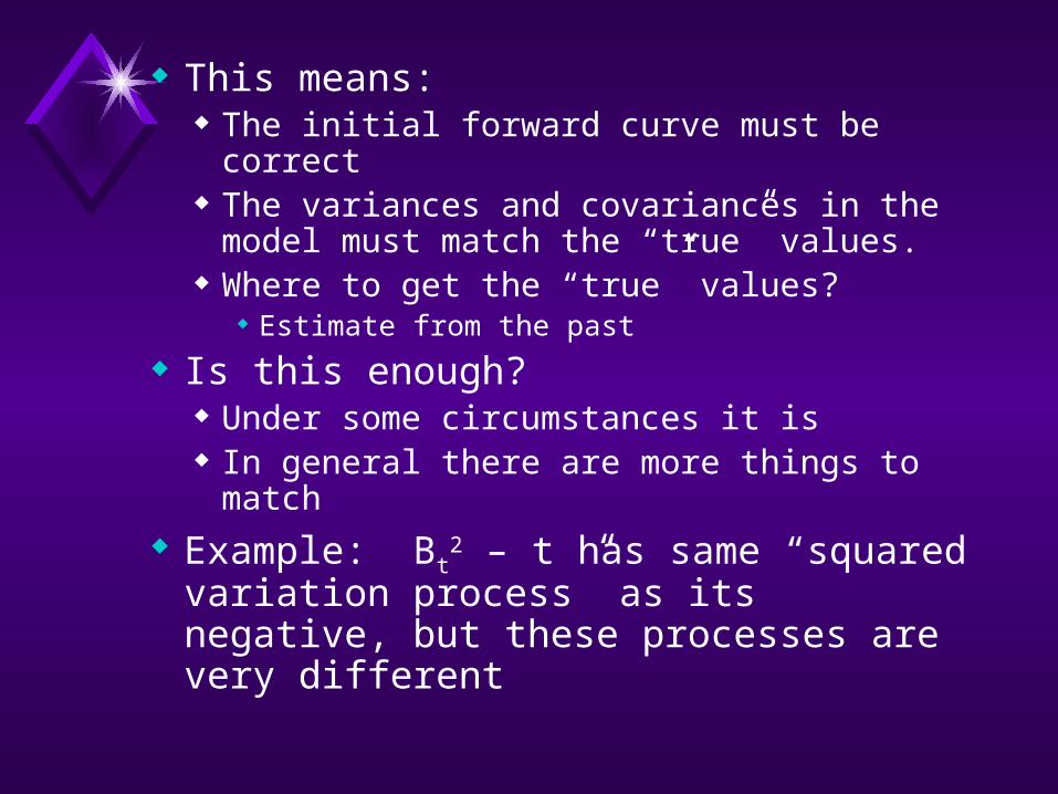
This means: The initial forward curve must be correct The variances and covariances in the model

must match the “true” values. Where to get the “true” values?

Estimate from the past

Is this enough? Under some circumstances it is In general there are more things to match

Example: Bt2 – t has same “squared

variation process” as its negative, but these processes are very different

SummarySummary

d

i

T

t

iit dtduutTttWdTtTtfd1

),,(),,()(~

),,(),,(

•Need to choose

•Initial forward curve

•Volatility functions

•These are the same for the physical measure as for the pricing measure

0 allfor ),0( TTf

,, allfor ),,( TtTt

Too much to choose!Too much to choose!

Actually, choosing f(0,) is often easy: From Treasury strips, or From Treasury bonds, or From swaps curve

It’s tougher in some “smaller” markets Not enough bonds Markets not liquid Bonds may have special features

Choosing Choosing For each T we must choose an adapted

stochastic process for These must vary smoothly with respect to T Narrowing down a useful

Limit dependence on :

),,(),( Ttt iTi

)OK! NOT ,like"-Black(" ),,(),( or

CIR) ofion (modificat ),,(),( or

CIR)in (as ),,(),( or

),(),,(

*

*

*

*

TtfTt

TtfTt

ttfTt

TtTt

i

i

i

ii

Still too much freedom?Still too much freedom?

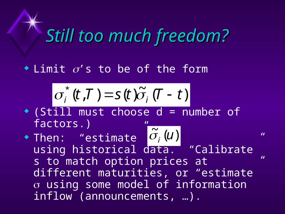
Limit ’s to be of the form

(Still must choose d = number of factors.) Then: “estimate” the using

historical data. “Calibrate” s to match option prices at different maturities, or “estimate” using some model of information inflow (announcements, …).

)(~)(),(* tTtsTt ii

)(~ ui

The resulting model form:The resulting model form:

is determined by “model choice” s is to permit adjustment for “implied

volatility” d (the number of factors) and the are

estimated from historical data The drift under the martingale measure is

determined by the above choices

d

iiit dtdrifttWdtTtstfTtfd

1

)(~

)(~)()),,((),,(

i~

An unfortunate factAn unfortunate fact I’d like to choose Unfortunately, the resulting equation

has the property that solutions explode with positive probability in any time interval

(Think of simpler equation y’=ky2.) We therefore use

),,()),,(( TtfTtf

dtdutuutftTTtfWdtTTtfTtfdT

t

ii

d

i

d

iiit

)(~),()(~),(~

)(~),(),(11

)),(,min()),(( TtfMTtf

How we estimate the modelHow we estimate the model

We assume we have values of historical forward curves

We choose M to be larger than any forward rate in our data set.

We discretize our evolution equation to get

KkJjtttfttf kjjkjj ,...,1;,...,1,),(),,(

dttWtTtsTtf

Ttf d

iii

t )junk()()(~)(),(

),(

1

Written in terms of our dataWritten in terms of our data

Now define the column vector X(j) so that its kth component, , is given by the above expression. These X’s are, of course, random

Now compute the natural estimator for the variance-covariance matrix of the X’s:

It’s the matrix V whose (k1,k2) entry is:

d

ijiki

j

kj

kjjkjj tWt

ts

ttf

ttftttf

1

)(~

)(~)(

),(

),(),(

)( jkX

J

j

jk

jkkk XX

Jv

1

)()(, .

12121

The expected value is given by:

We can, without loss of generality, pretend that the first term is equal to 1 (since that can change our results only by a multiplicative constant, and we can “adjust” the s() we’ll use to compensate for that).

J

j

jk

jkkk XXE

JvE

1

)()(, 2121

1

J

j

d

ikikijts

J 1 1

2 ).(~)(~)(1

21

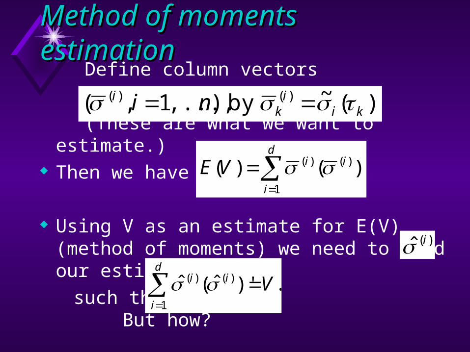
Method of moments estimationMethod of moments estimation Define column vectors

(These are what we want to estimate.) Then we have

Using V as an estimate for E(V) (method of moments) we need to find our estimates

such that But how?

).(~by ),...,1,( )()(ki

ik

i ni

d

i

iiVE1

)()( )'()(

)(ˆ i

.)'ˆ(ˆ1

)()(

d

i

ii V

Facts about matricesFacts about matrices

Definition: A square matrix B is positive definite provided x’Bx>0 whenever x is a column vector not equal to 0. It’s positive semidefinite if x’Bx 0 for all x.

Fact: Our V will always be positive semidefinite, and will almost always be positive definite.

Principal componentsPrincipal components

If V is a symmetric real positive definite matrix then there are matrices U and such that: is a diagonal matrix with diagonal entries positive and

non-increasing

UU’=I (the identity matrix)

V=UU’

Set T=U0.5. IF Z is a column vector of independent standard normal random variables,

then the variance-covariance matrix of TZ is V

More factsMore facts

The columns of U are called the “principal components” of V.

The “best” lower-dimensional approximation to the distribution of X results from replacing the “right-most” columns of U by 0.

“Best” means, in a particular sense, “minimal mean-squared error.”

No error analysis so far!No error analysis so far!

Recall: In theory one can calculate the variance-covariance structure exactly from any short evolution of the forward curve (using finer and finer subdivisions).

With a fixed sample, we can’t do that. Let’s look at a simpler problem: estimating

the variance of a random variable known to be normally distributed, mean 0, unknown variance

Suppose y1, …, yn are independent observations from an N(0,2) distribution

The natural estimator for 2 is

What is the standard error? It’s

Thus with n=50 observations, we typically get about 20% error in 2, which means about 10% in and in at-the-money option prices. Conclusion: we need lots of observations!

n

iiy

n 1

22 .1̂

nse

2)ˆ( 22

Trying this with real dataTrying this with real data We make a further discretization. We fit

the forward curve in a “piecewise flat” way: We think of discrete (relative) maturities of 0,

0.25, 0.5, 1.0, 2.0, 3.0, 5.0, 7.0 and 9.8 years. We use a forward curve which is constant between these maturities and select one k from each resulting interval.

For the “forward curve at the end” we keep the “endpoints” at the same “absolute dates”.

We do this for lots of values of tj.

We set “dt” to be one week.

Our dataOur data

We were given data about “forward Libor” rates. The next slide has an example of this data for observation date March 8, 1991.

In each row, the entries are: The date of a start of a “quarter” The number of days in this quarter The “actual daycount over 360” rate rate for

this quarter

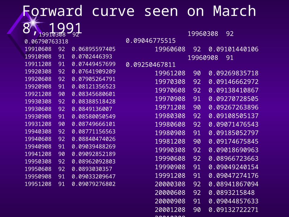
19910308 92 0.06790763318

19910608 92 0.0689559740519910908 91 0.070244639319911208 91 0.0744945769919920308 92 0.0764190920919920608 92 0.0790526479119920908 91 0.0812135652319921208 90 0.0834568060119930308 92 0.0838851842819930608 92 0.084913600719930908 91 0.0858005054919931208 90 0.0874966610119940308 92 0.0877115656319940608 92 0.0884047402619940908 91 0.0903948826919941208 90 0.0909285218919950308 92 0.0896209280319950608 92 0.089303035719950908 91 0.0903320964719951208 91 0.09079276802

19960308 92 0.0904677551519960608 92 0.09101440106

19960908 91 0.0925046781119961208 90 0.0926983571819970308 92 0.0914666297219970608 92 0.0913841086719970908 91 0.0927072850519971208 90 0.0926726389619980308 92 0.0910850513719980608 92 0.0907147654319980908 91 0.0918505279719981208 90 0.0917467584519990308 92 0.0901869096319990608 92 0.0896672366319990908 91 0.0904924015419991208 91 0.0904727417620000308 92 0.0894186709420000608 92 0.089321584820000908 91 0.0904485763320001208 90 0.0913272227120010308

Forward curve seen on March 8, 1991

Computing forward ratesComputing forward rates

For the week from tk to tk+1:

At tk compute the piecewise-flat continuously-compounded interest rate “explaining” the prices of pure discount bonds maturing at tk+0.25, tk+0.5, tk+1, tk+2, tk+3, tk+5, tk+7, and tk+9.8 years.

Similarly, at tk+1, compute rates for bonds maturing at tk+0.25, tk+0.5, tk+1, tk+2, tk+3, tk+5, tk+7, and tk+9.8 years. (The same absolute dates!)

Results for tResults for tkk=June 5, 1991=June 5, 1991

At the start of the week.06147114853932487.06418599716067086.07028591418277555 .07894618023869922 .08562248112095414 .09197819566016921 .09200485752193654 .09005201517594776 

At the end of the week .06282817092590599 .06547295594397448 .07270227193025801 .08144837689395647 .08688266008163854 .09130940580147720 .09348600859670100 .09060552897329775

Now we compute Now we compute f/f, gettingf/f, getting

0.02207576105

0.02005046023

0.03437897587

0.03169496799

0.01471785148

-0.007271178282

0.01609861821

0.006146600898

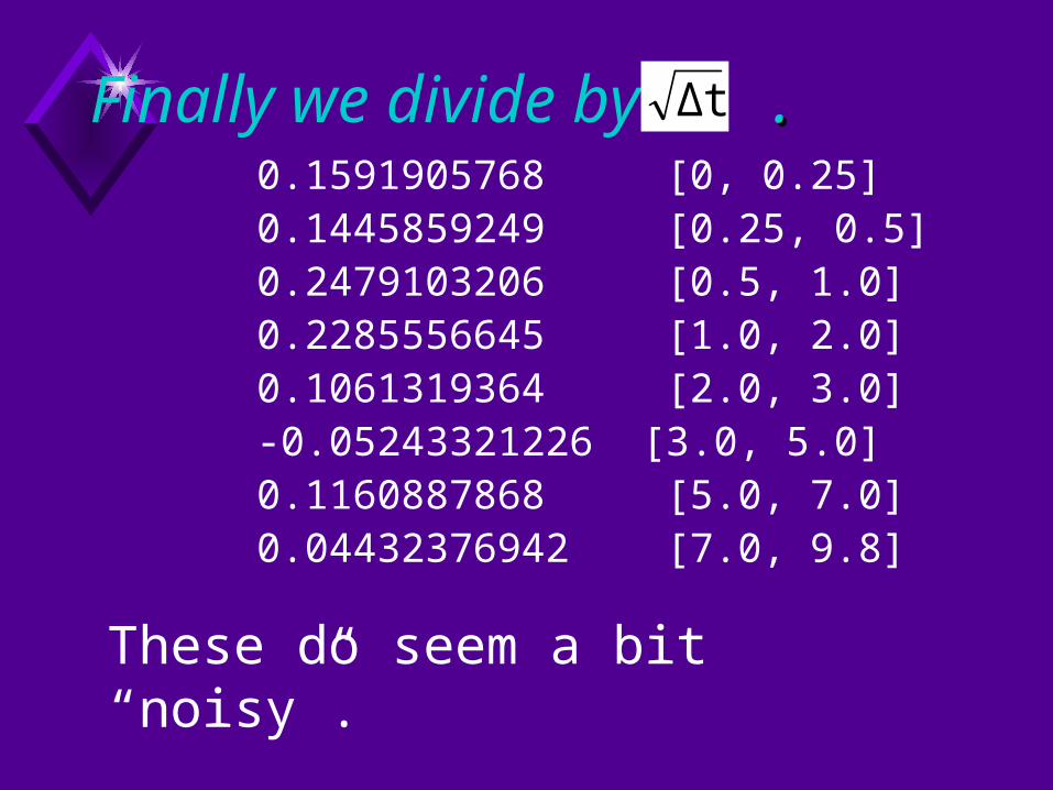
Finally we divide by . .0.1591905768 [0, 0.25] 0.1445859249 [0.25, 0.5] 0.2479103206 [0.5, 1.0]0.2285556645 [1.0, 2.0] 0.1061319364 [2.0, 3.0]-0.05243321226 [3.0, 5.0]0.1160887868 [5.0, 7.0]0.04432376942 [7.0, 9.8]

These do seem a bit “noisy”.

Δt

That was just one “X-vector”.That was just one “X-vector”.

We need to do this for each week. (I had about 5 years’ worth of data.)

With 5*52, or about 250 data points we could estimate variances with standard errors of about 9% (and sd’s with 4.5%)

We then need to estimate the variance-covariance matrix from these observations

Estimated variance-Estimated variance-covariance matrixcovariance matrix

0.02899 0.02016 0.02336 0.01810 0.01051 0.00756 0.00386 0.00289

0.02016 0.03267 0.03625 0.02769 0.01613 0.01353 0.00739 0.00551

0.02336 0.03625 0.05308 0.04384 0.02720 0.02354 0.01520 0.01114

0.01810 0.02769 0.04384 0.03972 0.02584 0.02163 0.01441 0.01086

0.01051 0.01613 0.02720 0.02584 0.02023 0.01737 0.01239 0.00972

0.00756 0.01353 0.02354 0.02163 0.01737 0.02447 0.00895 0.00766

0.00386 0.00739 0.01520 0.01441 0.01239 0.00895 0.03180 0.01066

0.00289 0.00551 0.01114 0.01086 0.00972 0.00766 0.01066 0.02508

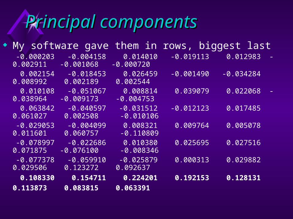
Principal componentsPrincipal components My software gave them in rows, biggest last -0.000203 -0.004158 0.014010 -0.019113 0.012983 -0.002911 -0.001068 -

0.000720 0.002154 -0.018453 0.026459 -0.001490 -0.034284 0.008992 0.002189

0.002544 0.010108 -0.051067 0.008814 0.039079 0.022068 -0.038964 -0.009173 -

0.004753 0.063842 -0.040597 -0.031512 -0.012123 0.017485 0.061027 0.002508 -

0.010106 -0.029053 -0.004099 0.008321 0.009764 0.005078 0.011601 0.060757 -

0.110809 -0.078997 -0.022686 0.010380 0.025695 0.027516 0.071875 -0.076100 -

0.008346 -0.077378 -0.059910 -0.025879 0.000313 0.029882 0.029506 0.123272

0.092637

0.108330 0.154711 0.224201 0.192153 0.128131 0.113873 0.083815

0.063391

11stst Principal Component Principal Component

0

0.05

0.1

0.15

0.2

0.25

0 1 2 3 4 5 6 7 8 9 10

Maturity

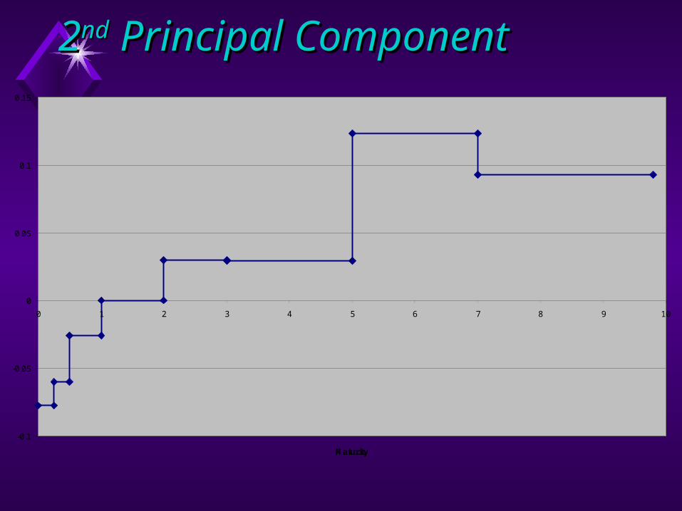
22ndnd Principal Component Principal Component

-0.1

-0.05

0

0.05

0.1

0.15

0 1 2 3 4 5 6 7 8 9 10

Maturity

How important are How important are multifactor models?multifactor models?

To check this we analyze two sets of problems with single- and multi-factor models

Problem 1: Caplets Problem 2: Swaps with optionality

The capletsThe caplets

For each year y from 1 to 9, consider an interest rate cap with only one period: It is effective precisely from (now plus y years) until (now plus y plus 0.25 years). The cap level is 6% (using actual/360), and the initial forward curve is flat at 6% (continuously compounded).

The swapsThe swaps

Consider a swap with two floating rate payers. Every six months from now until ten years are up

(except the first period) Payer 1 pays interest at the 6 month Tbill rate on a

notional of $1,000,000. Payer 2 pays similarly, but at the smaller of: the Tbill rate the yield of a 10 year CMT + b basis points.  We consider contracts with b varying from -80 to +20. The initial forward curve is upward sloping, starting at

6% and rising at 0.08% per year.

The modelsThe models

Ho and Lee: = constant Vasicek: (u)=c exp(-u) HJM “Old 1-factor” HJM “Old 2-factor” HJM “Adjusted 1 factor”

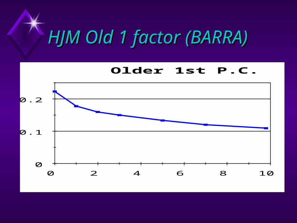
HJM Old 1 factor (BARRA)HJM Old 1 factor (BARRA)

0

0.1

0.2

0 2 4 6 8 10

Older 1st P.C.

HJM Old second factorHJM Old second factor

-0.15

-0.05

0.05

0.15

0 2 4 6 8 10

Older 2nd P.C.

0

0.005

0.01

0 5 10 15 20 Relative maturity

(HJM 1)*0.06 Vasicek, c=.0114, l=.0303

Choosing Vasicek fit

For Ho-Lee use = .01.

““HJM Adjusted”HJM Adjusted”

Effort is to get volatility at of each forward rate correct. (Correlations will be wrong, of course.)

HJM Adjusted =

((HJM 1)^2 + (HJM 2)^2) ^ 0.5

500

1000

1500

2000 V

alu

e

1 2 3 4 5 6 7 8 9 Years until start

Ho Lee Vasicek

HJM 1 factor Adjusted 1 factor

HJM 2 factor

Caplets

0

10000

20000

30000

Valu

e

-80 -60 -40 -20 0 20 BPs to add to 10 yr CMT yield

Ho Lee Vasicek

HJM 1 factor Adjusted 1 factor

HJM 2 factor

Swaps