consistency problems for hjm interest rate modelsjanroman.dhis.org/finance/hjm/roubustness in...
TRANSCRIPT

Diss. ETH No. 13603
Consistency Problemsfor
HJM Interest Rate Models
A dissertation submitted to theSWISS FEDERAL INSTITUTE OF TECHNOLOGY
ZURICH
for the degree ofDr. sc. math.
presented byDAMIR FILIPOVIC
Dipl. Math. ETHborn March 26, 1970
citizen of Schmiedrued AG
accepted on the recommendation ofProf. Dr. F. Delbaen, examiner
Prof. Dr. P. Embrechts, co-examiner
2000


Contents
Abstract iii
Introduction 1
Part 1. The HJM Methodology 7
Chapter 1. Stochastic Equations in Infinite Dimensions 91.1. Infinite Dimensional Brownian Motion 91.2. The Stochastic Integral 111.3. Fundamental Tools 131.4. Stochastic Equations 16
Chapter 2. The HJM Methodology Revisited 192.1. The Bond Market 192.2. The Musiela Parametrization 202.3. Arbitrage Free Term Structure Movements 242.4. Contingent Claim Valuation 28A Summary of Conditions 322.5. What Is a Model? 32
Chapter 3. The Forward Curve Spaces Hw 353.1. Definition of Hw 353.2. Volatility Specification 403.3. The Yield Curve 413.4. Local State Dependent Volatility 423.5. Functional Dependent Volatility 453.6. The BGM Model 46
Chapter 4. Consistent HJM Models 514.1. Consistency Problems 514.2. A Simple Criterion for Regularity of G 534.3. Regular Exponential-Polynomial Families 544.4. Affine Term Structure 58
Part 2. Publications 63
Chapter 5. A Note on the Nelson–Siegel Family 655.1. Introduction 655.2. The Interest Rate Model 665.3. Consistent State Space Processes 675.4. The Class of Consistent Ito Processes 69
i

ii CONTENTS
5.5. E-Consistent Ito Processes 73
Chapter 6. Exponential-Polynomial Families and the Term Structure ofInterest Rates 75
6.1. Introduction 756.2. Consistent Ito Processes 776.3. Exponential-Polynomial Families 786.4. Auxiliary Results 816.5. The Case BEP (1, n) 846.6. The General Case BEP (K,n) 866.7. E-Consistent Ito Processes 926.8. The Diffusion Case 936.9. Applications 956.10. Conclusions 97
Chapter 7. Invariant Manifolds for Weak Solutions to Stochastic Equations 997.1. Introduction 997.2. Preliminaries on Stochastic Equations 1017.3. Invariant Manifolds 1057.4. Proof of Theorem 7.6 1067.5. Proof of Theorems 7.7, 7.9 and 7.10 1107.6. Consistency Conditions in Local Coordinates 113
Appendix: Finite Dimensional Submanifolds in Banach Spaces 115
Bibliography 121

Abstract
This thesis brings together estimation methods and stochastic factor modelsfor the term structure of interest rates within the HJM framework. It is based onthe complex of consistency problems introduced by Bjork and Christensen [7].
There exist commonly used methods for fitting the current term structure.Any curve fitting method can be represented as a parametrized family of smoothcurves G = G(·, z) | z ∈ Z with finite dimensional parameter set Z. A lotof cross-sectional data z is available, and one may ask for a suitable stochasticmodel for z which provides accurate bond option prices. However, this requiresthe absence of arbitrage. We characterize all consistent Z-valued state space Itoprocesses Z which, by definition, provide an arbitrage-free model when representingthe parameter z. Obviously, G(T − t, Zt) has to satisfy the HJM drift condition.It turns out that selected common curve fitting methods do not go well with theHJM framework.
We then consider the preceding consistency problem from a geometric point ofview, as proposed by Bjork and Christensen [7]. We extend the HJM framework toincorporate an infinite dimensional driving Brownian motion. We then perform thechange of parametrization due to Musiela [37] and arrive at a stochastic equation ina Hilbert space H , describing the arbitrage-free evolution of the forward curve. Thefamily G can be treated as a subset of H and the above consistency considerationsyield a stochastic invariance problem for the previously derived stochastic equation.Under the assumption that G is a regular submanifold of H , we derive sufficientand necessary conditions for its invariance. Expressed in local coordinates theyturn out to equal the HJM drift condition.
Classical models, such as the Vasicek [48] and CIR [17] short rate model, andthe popular BGM [12] LIBOR rate model, are shown to fit well into that framework.By their very definition, affine HJM models are consistent with finite dimensionallinear submanifolds of H . A straight application of our results yields a completecharacterization of them, as obtained by Duffie and Kan [21].
In conclusion, we provide a general tool for exploiting the interplay betweencurve fitting methods and HJM factor models.
iii

Introduction
Bond markets differ in one fundamental aspect from standard stock markets.While the latter are built up by a finite number of traded assets, the underlyingbasis of a bond market is the entire term structure of interest rates: an infinitedimensional variable which is not directly observable. On the empirical side thisnecessitates curve fitting methods for the daily estimation of the term structure.Pricing models on the other hand, are usually built upon stochastic factors repre-senting the term structure in a finite dimensional state space.
The aim of this thesis is threefold: to bring together estimation methods andfactor models for interest rates, to provide appropriate consistency conditions andto explore some important examples.
By a bond with maturity T we mean a default-free zero coupon bond withnominal value 1. Its price at time t is denoted by P (t, T ). There is a one to onerelation between the time t term structure of bond prices and the time t termstructure of interest rates or forward curve f(t, T ) | T ≥ t given by
P (t, T ) = exp
(−∫ T
t
f(t, s) ds
).
Accordingly, f(t, T ) is the continuously compounded instantaneous forward ratefor date T prevailing at time t. The forward curve contains all the necessaryinformation for pricing bonds, swaps and forward rate agreements of all maturities.Furthermore, it is a vital indicator for central banks in setting monetary policy.
Several algorithms for constructing the current term structure of interest ratesfrom market data are applied in practice. A recent document from the Bank forInternational Settlements (BIS [6]) provides an overview of all estimation methodsused by some of the most important central banks, see Table 1 on page 76. Promi-nent among them are the curve fitting procedures by Nelson and Siegel [39] andSvensson [44] and smoothing splines. Any common method can be represented asa parametrized family G = G(·, z) | z ∈ Z of smooth curves where Z ⊂ Rm is afinite dimensional parameter set (m ∈ N). By appropriate choice of the parameterz ∈ Z, an optimal fit of the forward curve x 7→ G(x, z) to the observed data isachieved. Here x ≥ 0 denotes time to maturity. In that sense z represents thecurrent state of the economy, taking values in the state space Z.
According to [6] a lot of cross-sectional data, i.e. daily estimations of z, isavailable for selected estimation methods G. In addition there exists an exten-sive literature on statistical inference for diffusion processes based on discrete timeobservations, see e.g. [5]. It therefore seems promising to explore the stochasticevolution of the parameter z continuously over time.
1

2 INTRODUCTION
Henceforth we are given a complete filtered probability space (Ω,F , (Ft)t∈R+ ,P)satisfying the usual conditions. Let Z = (Zt)t∈R+ be a diffusion model for the aboveparameter z. One would think that now f(t, T ) = G(T −t, Zt) provides an accuratefactor model for the interest rates. However, there are constraints on the dynamicsof Z, such as the requirement of absence of arbitrage. By this we mean the existenceof a probability measure Q ∼ P under which discounted bond price processes followlocal martingales (Q is called an equivalent local martingale measure or risk neutralmeasure). Necessary conditions can be formulated in terms of the generator of Zapplied to G. These conditions turn out to be very restrictive. ForG fixed we arriveat a type of inverse problem for the generator of Z. State space processes Z whichcomply with these constraints, are called consistent with G. It can be shown forexample that the Nelson–Siegel family admits no non-trivial consistent diffusionZ. We achieve these negative results even for generic state space Ito processesZ (thereby the inverse problem applies to the characteristics of Z instead of thegenerator as for diffusions).
An application of Ito’s formula shows that the preceding approach is part ofthe framework introduced by Heath, Jarrow and Morton (henceforth HJM) [28]which basically unifies all continuous interest rate models. For arbitrary but fixedT ∈ R+, HJM let f(·, T ) evolve as an Ito process
f(t, T ) = f(0, T ) +∫ t
0
α(s, T ) +∫ t
0
σ(s, T ) dWs, t ∈ [0, T ]. (1)
Originally in [28], W is a finite dimensional Brownian motion. We will however ex-tend this approach at once by considering an infinite dimensional Brownian motionW . This generalization is straightforward but one has to take care of the definitionof the stochastic integral.
The no-arbitrage requirement cumulates in the well-known HJM drift condi-tion: existence of an equivalent local martingale measure Q yields a representationfor the Q-drift of f(·, T ) in terms of σ. Thus, pricing formula for interest rate sensi-tive contingent claims do only depend on σ. The above mentioned inverse problemfor the characteristics of Z is simply this drift condition.
Note that (1) provides a generic description of the arbitrage-free evolutionrather than a model for the interest rates. By HJM’s result it is convenient andstandard to describe the evolution of f(·, T ) under the risk neutral measure Q,involving only σ and the Girsanov transform W of W .
Musiela [37] proposed the reparametrization
rt(x) = f(t, x+ t), (2)
taking better into account the nature of the forward curve x 7→ rt(x) as an (infinitedimensional) state variable, where x ≥ 0 denotes time to maturity. We ask: whatis the implied stochastic dynamics for (rt(x))t∈R+?
The semigroup theory for stochastic equations in a Hilbert space provided byDa Prato and Zabczyk [18] is tailor-made for that approach. We give an axiomaticscheme for the choice of an admissible Hilbert space H of functions h : R+ → R inwhich (rt)t∈R+ can be realized as a solution to the stochastic equation
drt = (Art + FHJM (t, rt)) dt+ σ(t, rt) dWt
r0 = h0.(3)

INTRODUCTION 3
Here A is the generator of the semigroup of right-shifts S(t)h(x) = h(x + t). Thecoefficients1 σ = σ(t, ω, h) and FHJM = FHJM (t, ω, h) are random mappings. Thelatter is fully specified by σ according to the HJM drift condition under the measureQ (under P the market price of risk is also involved). Equation (3) with h0 = f(0, ·)represents the system of infinitely many Ito processes (1) as one dynamical systemin infinite dimensions, now allowing for arbitrary initial curves r0 ∈ H .
The axiomatic exposure of an admissible Hilbert space of forward curves isnew. We propose a particular class of admissible Hilbert spaces, which are botheconomically reasonable and appropriate for providing existence and uniquenessresults for (3) in full generality. Any Lipschitz continuous and bounded volatilitycoefficient σ provides an HJM model therein. Classical models are shown to fit wellinto that framework. These include the short rate models of Vasicek [48] and Cox,Ingersoll and Ross (henceforth CIR) [17], and also the popular LIBOR model byBrace, Gatarek and Musiela (henceforth BGM) [12].
Equation (3) was introduced and analyzed first in [37] and [13], but onlyfor deterministic volatility structure. In that Gaussian framework Musiela alsocharacterized the set of attainable forward curves by the model. This is an issuewhich is strongly related to the present discussion. Further aspects of equation (3)have been exploited by several authors. Among them are Bjork et al. [7], [8], [10],Zabczyk [50], Vargiolu [47], [46] and Milian [34]. Research is ongoing. A rigorousexposure of the no-arbitrage property for equation (3) as provided by this thesistherefore seems to be needed.
In view of the previously mentioned negative consistency results for commonestimation methods, one can proceed in two possible ways. Either one consid-ers more general non-continuous (Markovian) state space processes Z, or one stayswithin the continuous (that is HJM) regime and looks for appropriate forward curvefamilies G. The first approach is not a topic of this thesis and will be exploitedelsewhere, see [26]. The second approach leads naturally to the complex of con-sistency problems for HJM models introduced by Bjork and Christensen [7]. Theypropose the following geometric point of view.
Considering G as a subset of H , we can study the stochastic invariance problemrelated to (3) for G. The set G is called (locally) invariant for (3) if for any space-time initial point (t0, h0) ∈ R+ × G, the solution r = r(t0,h0) of (3) stays (locally)in G almost surely. Accordingly, we call the HJM model provided by (3) consistentwith G.
By a solution to (3) we mean a mild or weak solution rather than a strongsolution. These three concepts will be defined below, see Definition 1.19. It isessential, however, to notice that a mild or a weak solution is not an H-valuedsemimartingale.
The existence of a state space diffusion process Z which is (locally) consistentwith G for any initial point (t0, z0) ∈ R+ × Z obviously implies consistency of theinduced HJM model G(·, Z) with G. The converse is not true in general: if themodel (3) is consistent with G it’s not clear what the Z-valued coordinate processZ determined by
G(·, Zt) = rt (4)
1By a slight abuse of notation we use the same letter σ in (3) as well as (1), although theyrepresent different objects.

4 INTRODUCTION
looks like. We cannot expect it to be an Ito process.We provide a general regularity result for this problem. Suppose G is a finite
dimensional regular submanifold ofH and locally invariant for a stochastic equationlike (3). Then the coordinate process Z in (4) is a Z-valued diffusion. Furthermore,we find Nagumo-type consistency conditions in terms of σ and FHJM and thetangent bundle of G. Expressing these consistency conditions in local coordinates wearrive at exactly the above inverse problem for the characteristics of the coordinate(i.e. state space) process Z. That way the consistency problem for G is completelysolved.
These results are then applied to the estimation methods provided by [6]. Undersome technical restrictions, we show that exponential-polynomial families , such asthose of Nelson–Siegel or Svensson, are regular submanifolds of H . Thus, thepreviously derived negative consistency results can be restated within the presentsetup.
A further application yields the characterization of all HJM models which areconsistent with linear submanifolds. These are just the affine HJM models. Wederive the well-known results of Duffie and Kan [21] from our general point of view.
The present consistency results have been basically established by Bjork andChristensen [7]. However, they proceeded under much stronger assumptions whichare not necessarily convenient for the HJM framework, see Remark 2.16 below.Moreover, they did not address the difference between a regular and an immersedsubmanifold, see Figure 1 on page 52. By exploiting the strong structure of theregular submanifold G we derive global invariance results in contrast to [7] whereonly local results are provided. New is also the representation of the consistencyconditions in local coordinates, making them feasible for applications, which workmainly in one direction: given a curve fitting method G, we can determine theconsistent HJM models. The converse problem of the existence of an invariant finitedimensional submanifold, given a particular HJM model, is treated in Bjork andSvensson [10], by using the Frobenius theorem. The non-consistency of exponential-polynomial families has been proved in [7] for the particular case of a deterministicvolatility structure.
Similar stochastic invariance problems have been studied by Zabczyk [50],Jachimiak [30] and for finite dimensional systems by Milian [33] (see also the refer-ences therein). Bjork et al. [8], [10] discuss further the existence of (minimal) finitedimensional realizations for (3). In [50] the invariance question for finite dimen-sional linear subspaces with respect to Ornstein–Uhlenbeck processes is resolved.Applications to HJM models, the BGM model and to a second order term struc-ture model by Cont [16] are exploited. But the support theorem methods in [50]have not yet been established for the general equation (3). Jachimiak [30] exploitsinvariance for closed sets K ⊂ H . However, his methods cannot be applied directlyto (3).
Outline. The thesis is divided into two parts. Part 2 contains a series ofthree articles ([25], [23], [24]) developed during my Ph.D. research over the lastthree years. All have been accepted for publication by renowned journals. Part 1represents a synthesis of the three articles cumulating in the central Chapter 4.

INTRODUCTION 5
In Chapter 1 we repeat the relevant material from [18] about stochastic anal-ysis in infinite dimensions. We define an infinite dimensional Brownian motionW and show how it can be realized as Hilbert space valued Wiener process. Theconstruction of the stochastic integral with respect to W is then sketched and weprovide the main tools from stochastic analysis: Ito’s formula, the stochastic Fubinitheorem and Girsanov’s theorem. We introduce stochastic equations in a Hilbertspace, define the concepts for a solution and state an existence and uniquenessresult.
Chapter 2 recaptures the HJM [28] methodology and extends it to incorporatean infinite dimensional driving Brownian motion W . We perform the change ofparametrization (2) and arrive at the stochastic equation (3) in a Hilbert spaceH which is axiomatically scheduled. The no-arbitrage (or HJM drift) condition isrigorously exposed. We give a sketch for contingent claim valuation in the precedingbond market and discuss in particular the forward measure, forward LIBOR ratesand caplets. This is introductory for the BGM model to be recaptured in thesubsequent chapter. Finally, we define what we mean by an HJM model.
In Chapter 3 we introduce a class of Hilbert spaces Hw which are both eco-nomically reasonable and convenient for analyzing the previously derived stochasticequation (3). We provide a general existence and uniqueness result for Lipschitzcontinuous and bounded volatility coefficients σ. Classical models are shown to fitwell into that framework. So is the classical HJM model which corresponds to lo-cally state dependent volatility coefficients σ. We also recapture the popular BGMmodel and provide further promising examples.
Chapter 4 is central and can be considered as the main chapter. It unifies theresults obtained in [25], [23] and [24] within the previously constructed framework.We state the main result for regular families G and thus solve completely the consis-tency problem. We discuss some pitfalls which arise from the subtle but importantdifference between a regular and an immersed submanifold. A simple criterionfor differentiability in Hw is presented and applied to the class of exponential-polynomial families. We restate the (negative) consistency results for the commonNelson–Siegel and Svensson families. Finally, we apply our methods for identifyingthe class of affine term structure models which are characterized by possessing lin-ear invariant submanifolds. We provide some of the well-known results from [21]and recapture the Vasicek and CIR short rate models.
Chapter 5 is [25] and shows that there exists no non-trivial state space Itoprocess which is consistent with the Nelson–Siegel family.
Chapter 6 is [23]. Here we extend the methods used in Chapter 5 for char-acterizing the class of state space Ito processes which are consistent with generalexponential-polynomial families. We obtain remarkably restrictive results. In par-ticular we identify the only non-trivial HJM model which is consistent with theSvensson family: an extended Vasicek short rate model. Chapters 5 and 6 weremotivated by the examples given in [7], see Remarks 5.3 and 7.1 therein.
Chapter 7 is an extended version (with an additional section and completeproofs) of [24]. It is not directly related to interest rate models and providesgeneral results on stochastic invariance for finite dimensional submanifolds in aHilbert space. The main results of [7] are considerably extended.
The appendix includes a comprehensive discussion on finite dimensional sub-manifolds in Banach spaces. Their crucial properties are deduced.

6 INTRODUCTION
Remark on Notation. Basically, we follow the notation of [40] and [18].Let G and H be Banach spaces. The norm of H is denoted by ‖ · ‖H and we
write B(H) for the σ-algebra generated by its topology. If H is a Hilbert space weuse the notation 〈·, ·〉H for its scalar product. The closure of a subset M ⊂ H isdenoted by M . We define the open ball of radius R > 0
BR(H) := h ∈ H | ‖h‖H < R.The space of continuous linear operators from G into H is denoted L(G;H)
and L(H) = L(H ;H) for short. We write D(A) for the domain of an (unbounded)linear operator A : G→ H and A∗ for its adjoint.
We write C(G;H) and Ck(G;H) for the space of continuous and k times con-tinuously differentiable mappings φ : G → H , respectively. The derivatives aredenoted by Dφ and Dkφ.
For U ⊂ Rm, m ∈ N, the space of continuous, resp. k times continuouslydifferentiable functions f : U → R is written shortly C(U), resp. Ck(U), andCkc (U) consists of those elements of Ck(U) which have compact support in U .
If (Ω,F ,P) is a measure space and p ≥ 1, we write Lp(Ω,F ,P) for the Banachspace of integrable functions2 X : Ω→ R equipped with norm
‖X‖pLp(Ω,F ,P) =∫
Ω
|X(ω)|p dP(ω).
If Ω is a Borel subset of R and P the Lebesgue measure, we just write Lp(Ω).The space of locally integrable functions3 h : Ω→ R is denoted by L1
loc(Ω).Letters such as C, C, K, . . . represent positive real constants which, if not
otherwise stated, can vary from line to line.All remaining notation is either standard and self-explanatory or it is intro-
duced and explained in the text.
Acknowledgements. It is a great pleasure to thank my adviser F. Delbaenfor his guidance throughout my Ph.D. studies. He has given me his time and hisinsights in the course of many stimulating conversations. I am very grateful tohim for his generosity and for giving me the opportunity of several educationalexcursions abroad.
I have profited from fruitful discussions with many people at several meetingsand seminars. Very special thanks go to T. Bjork and J. Zabczyk for their helpfuland motivating suggestions, and their hospitality, which have been essential forthe development of this thesis. I would like to thank also B. J. Christensen andG. Da Prato for their interest and hospitality. Furthermore, I thank P. Embrechtsfor being co-examiner.
Thanks go to Axel Schulze–Halberg, Paul Harpes, Freweini Tewelde, UweSchmock and all my colleagues from ETH for their friendship and support, andespecially to Manuela for her love over the last years.
Financial support from Credit Suisse is gratefully acknowledged.
2In fact, equivalence classes of functions where X ∼ Y if X = Y P-a.s.3That is, equivalence classes (h ∼ g if h = g a.s.) of measurable functions h satisfying∫
BR(R)∩Ω|h(x)| dx <∞ ∀R ∈ R+.

Part 1
The HJM Methodology


CHAPTER 1
Stochastic Equations in Infinite Dimensions
In this chapter we provide some introduction to infinite dimensional stochasticanalysis and sketch the relevant material from Da Prato and Zabczyk [18] withoutgiving detailed proofs. For terminology and notation we refer to [18] and [40].
Here and subsequently, (Ω,F , (Ft)t∈R+ ,P) stands for a complete filtered prob-ability space satisfying the usual conditions1. The predictable σ-field is denoted byP . We will suppress the notational dependence of stochastic variables on ω whenno confusion can arise.
Throughout, H denotes a separable Hilbert space.Let I ⊂ R+. A stochastic process (t, ω) 7→ Xt(ω) : I × Ω → H will be written
indifferently2 (Xt)t∈I , resp. X or (Xt) if there is no ambiguity about the indexset I. Whereas Xt : Ω→ H is a random variable for each t ∈ I.
Two processes (Xt)t∈I and (Yt)t∈I are indistinguishable if
P[Xt = Yt, ∀t ∈ I] = 1.
We do not distinguish between them and write X = Y .
1.1. Infinite Dimensional Brownian Motion
What is an H-valued “standard Brownian motion” W? A natural requirementwould be that 〈W,h〉H were a real Brownian motion with
E[〈Wt, h〉H〈Wt, h′〉H ] = t〈h, h′〉H , ∀h, h′ ∈ H.
If dimH <∞ this certainly applies. But in general
E[‖Wt‖2H
]=∑j∈N
E[|〈Wt, hj〉H |2
]=∑j∈N
t =∞
where hj | j ∈ N is an orthonormal basis in H . Whence Wt does not exist in H ,see [49]. Usually one relaxes the condition on Wt belonging to H . Yor [49] gives acomprehensive overview of the different concepts for defining W .
However, we will use a more direct approach here. For us, an infinite dimen-sional Brownian motion is a sequence
W = (βj)j∈N (1.1)
of independent real-valued standard (Ft)-Brownian motions. For being consistentwith [18] we show first how W can be realized as a Hilbert space valued Wienerprocess.
1F is P-complete, (Ft) is increasing and right continuous, F0 contains all P-nullsets of F2Differing notations like (B(t))t∈R+ or (P (t, T ))t∈[0,T ] are self-explanatory.
9

10 1. STOCHASTIC EQUATIONS IN INFINITE DIMENSIONS
For that purpose we introduce the usual Hilbert sequence space
`2 :=v = (vj)j∈N ∈ RN
∣∣∣∣ ‖v‖2`2 :=∑j∈N|vj |2 <∞
and denote by gj | j ∈ N the standard orthonormal basis3 in `2. As mentionedabove, W = (βj)j∈N ≡
∑j∈N β
jgj does not exist in `2. In the notation of [18,Section 4.3.1], W is a cylindrical Wiener process in `2. It can be realized in a largerspace as follows.
Let λ = (λj)j∈N be a sequence of strictly positive numbers with∑j λj < ∞.
We define the weighted sequence Hilbert space
`2λ :=v = (vj)j∈N ∈ RN
∣∣∣∣ ‖v‖2`2λ :=∑j∈N
λj |vj |2 <∞.
Clearly, `2 ⊂ `2λ with Hilbert–Schmidt embedding, and ej := (λj)−12 gj form an
orthonormal basis in `2λ. Define Q ∈ L(`2λ) by Qej := λjej . Obviously, the operatorQ is strictly positive, self-adjoint and nuclear. Moreover we have Q
12 (`2λ) = `2 and
Q−12 : `2 → `2λ is an isometry since for u, v ∈ `2
〈u, v〉`2 =∑j∈N
ujvj =∑j∈N
λjuj√λj
vj√λj
= 〈Q− 12u,Q−
12 v〉`2λ . (1.2)
Fix T ∈ R+.
Definition 1.1. We denote by H2T (H) the space of H-valued continuous mar-
tingales4 M on [0, T ] such that
‖M‖2H2T (H) := E
[‖MT‖2H
]<∞. (1.3)
Write M∗T := supt∈[0,T ] ‖Mt‖H . Doob’s inequality [18, Theorem 3.8] says
E[|M∗T |2
]≤ 4‖M‖2H2
T (H), for M ∈ H2T . (1.4)
Using (1.4) it can be shown as in [18, Proposition 3.9] that H2T (H) is a Hilbert
space for the norm (1.3). Denote by H0,2T (H) the closed subspace consisting of
M ∈ H2T (H) with M0 = 0.
We adopt the terminology of [18, Section 4.1].
Definition 1.2. An `2λ-valued continuous martingale X is called a Q-Wienerprocess if
i) X0 = 0ii) X has independent incrementsiii) Xt − Xs is centered Gaussian5 with covariance operator (t − s)Q, for all
0 ≤ s ≤ t.
Proposition 1.3. The series
W =∑j∈N
βjgj
converges in H0,2T (`2λ) for all T ∈ R+ and defines a Q-Wiener process in `2λ.
3That is, g1 = (1, 0, . . . ), g2 = (0, 1, 0, . . . ), . . .4see [18, Section 3.4]5see [18, Section 2.3.2]

1.2. THE STOCHASTIC INTEGRAL 11
Observe that this realization of W as a Hilbert space valued Wiener processdepends on the choice of λ. Indeed, the same procedure applies for any givensequence λ sharing the above properties. Yet the class of integrable processes doesnot depend on λ as we shall see.
Proof. Fix T ∈ R+. We define Wn ∈ H0,2T (`2λ) by
Wn =n∑j=1
βjgj, n ∈ N. (1.5)
Obviously, E[‖Wn
T −WmT ‖2`2λ
]= T
∑nj=m+1 λj → 0 for m,n→ 0. Hence (Wn)n∈N
is a Cauchy sequence inH0,2T (`2λ), converging to W . Since this holds for any T ∈ R+,
we get that W is an `2λ-valued continuous martingale.For any v ∈ `2λ the R-valued random variables 〈Wn
t −Wns , v〉`2λ are centered
Gaussian, converging in L2(Ω,F ,P) to 〈Wt −Ws, v〉`2λ which is therefore centeredGaussian too. By the same reasoning
E[〈Wt −Ws, ei〉`2λ〈Wt −Ws, ej〉`2λ
]= (t− s)〈Qei, ej〉`2λ .
Whence Condition iii) of Definition 1.2 holds. Similarly one shows ii) and clearlyW0 = 0.
Remark 1.4. We notice that any Hilbert space valued (cylindrical) Wiener pro-cess in the terminology of Da Prato and Zabczyk [18] can be considered in thepreceding RN-framework (1.1), see [18, Propositions 4.1 and 4.11].
1.2. The Stochastic Integral
For the definition of the stochastic integral with respect to W , Da Prato andZabczyk [18] introduce the space L0
2(H) of Hilbert Schmidt operators from `2 intoH .6 It consists of linear mappings Φ : `2 → H with
‖Φ‖2L02(H) :=
∑j∈N‖Φj‖2H <∞, (1.6)
where Φj := Φ(gj). In the sequel we shall identify Φ with (Φj)j∈N. On the otherhand, observe that any sequence (Φj)j∈N of H-valued predictable processes satis-fying (1.6) provides7 an L0
2(H)-valued predictable process Φ by Φ(gj) := Φj .Notice the particular case L0
2(R) = `2.
We summarize the construction of the stochastic integral, based on the theoryfrom [18, Sections 4.1-4.4]. Fix T ∈ R+.
Definition 1.5. We call L2T (H) the Hilbert space of equivalence classes of
L02(H)-valued predictable processes Φ with norm
‖Φ‖2L2T (H) := E
[∫ T
0
‖Φt‖2L02(H) dt
]. (1.7)
6Remember that `2 = Q12 (`2λ) endowed with the implied scalar product, see (1.2) and com-
pare with [18, (4.7)].7Notice that B(L0
2(H)) =⊗N B(H).

12 1. STOCHASTIC EQUATIONS IN INFINITE DIMENSIONS
Then there exists an isometry Φ 7→ Φ ·W between L2T (H) and H0,2
T (H), see[18, Proposition 4.5], defined on the dense8 subset of elementary L(`2λ;H)-valued9
processes
Φ =k−1∑m=0
Φm1(tm,tm+1], Φm is Ftm-measurable, (1.8)
by
(Φ ·W )t :=k−1∑m=0
Φm(Wtm+1∧t −Wtm∧t), t ∈ [0, T ].
Definition 1.6. The H-valued continuous martingale (Φ ·W )t∈[0,T ] is calledthe stochastic integral of Φ with respect to W and is also denoted by
(Φ ·W )t =∫ t
0
Φs dWs.
It is clear, how stochastic integration with respect to the d-dimensional Brow-nian motion W d = (β1, . . . , βd), d ∈ N, is included in this concept: any Hd-valuedpredictable process Φ = (Φ1, . . . ,Φd) can be considered as L0
2(H)-valued predictableprocess Φ by setting Φj = Φj if j ≤ d and Φj ≡ 0 for j > d. This way one getseasily
(Φ ·W d)t = (Φ ·W )t =d∑j=1
∫ t
0
Φjs dβjs . (1.9)
Here are some elementary properties of the stochastic integral. Denote by E aseparable Hilbert space.
Proposition 1.7. Let Φ ∈ L2T (H).
i) For any stopping time τ ≤ T
(Φ ·W )t∧τ = ((Φ1[0,τ ]) ·W )t. (1.10)
ii) The following series converges uniformly on [0, T ] in probability
(Φ ·W )t =∑j∈N
∫ t
0
Φjs dβjs . (1.11)
iii) Let A ∈ L(H ;E). Then A Φ ∈ L2T (E) and
A(Φ ·W ) = (A Φ) ·W. (1.12)
Proof. Property i) is [18, Lemma 4.9]. Property ii) follows by considering(1.9) and (Φ1, . . . ,Φd, 0, . . . ) which converges in L2
T (H) towards Φ for d → ∞.Now apply Doob’s inequality (1.4). Finally, iii) can be shown in the same way as[18, Proposition 4.15].
Notice that all equalities hold in H0,2T (H), hence up to indistinguishability.
There is a larger class of integrable processes than L2T (H).
8see [18, Proposition 4.7]9for an arbitrary choice of λ = (λj)j∈N as in Section 1.1

1.3. FUNDAMENTAL TOOLS 13
Definition 1.8. We call LlocT (H) the space of all L0
2(H)-valued predictable pro-cesses Φ such that
P
[∫ T
0
‖Φt‖2L02(H) <∞
]= 1.
Observe that Φ ∈ LlocT (H) if and only if there exists an increasing sequence of
stopping times τn ↑ T such that Φ1[0,τn] is in L2T (H) for all n ∈ N. This allows us
to extend the notion of the stochastic integral, see [18, p. 94–96].
Proposition 1.9. Let Φ ∈ LlocT (H). Then there exists a unique H-valued con-
tinuous local martingale (Mt)t∈[0,T ] characterized by
Mt∧τ = ((Φ1[0,τ ]) ·W )t
whenever Φ1[0,τ ] ∈ L2T (H). Again, M is called the stochastic integral of Φ with
respect to W and it is written
Mt =: (Φ ·W )t =∫ t
0
Φs dWs.
Many properties of the stochastic integral for L2T (H)-integrands carry over for
LlocT (H)-integrands by localization. Here is one feature of this method.
Lemma 1.10. Let (Mn)n∈N be a sequence of H-valued continuous local martin-gales. Assume that for all δ > 0 there exists a stopping time τ with P[τ < T ] ≤ δsuch that (Mn
t∧τ )→ 0 in H2T (H). Then (Mn)∗T → 0 in probability.
Proof. Let δ, ε > 0 and τ be as in the lemma. Then
P [(Mn)∗T > ε] ≤ δ + P
[supt∈[0,T ]
‖Mnt∧τ‖H > ε
]and the last term goes to zero as n→∞ by Doob’s inequality (1.4).
Using Lemma 1.10 the following can be shown.
Proposition 1.11. Equality (1.9) and Proposition 1.7 remain valid if L2T (H)
is replaced by LlocT (H).
Up to now, the stochastic integral was defined only on the finite time interval[0, T ]. But we can consider integrands in L2(H) := L2
∞(H) (with T in (1.7) replacedby ∞), respectively Lloc(H) :=
⋂T∈R+
LlocT (H).
Let Φ ∈ L2(H). Write Mn := Φ1[0,n] ·W for the stochastic integral on [0, n].By (1.10), Mn+1 coincides with Mn on [0, n] for all n ∈ N. Therefore we can defineunambiguously a process Φ·W – the stochastic integral of Φ with respect to W – bystipulating that it is equal to Mn on [0, n]. This process is obviously an H-valuedcontinuous martingale.
By localization the same procedure applies for Φ ∈ Lloc(H), and Φ ·W is anH-valued continuous local martingale.
1.3. Fundamental Tools
Three fundamental theorems of stochastic analysis are Ito’s formula, the sto-chastic Fubini theorem and Girsanov’s theorem. The first is given by Lemma 7.11.This section provides the other two.

14 1. STOCHASTIC EQUATIONS IN INFINITE DIMENSIONS
1.3.1. The Stochastic Fubini Theorem. Let (E, E) be a measurable spaceand let Φ : (t, ω, x) 7→ Φt(ω, x) be a measurable mapping from (R+×Ω×E,P⊗E)into (L0
2(H),B(L02(H))). In addition let µ denote a finite positive measure on (E, E).
Fix T > 0. By localization we get the following version of [18, Theorem 4.18].
Theorem 1.12 (Stochastic Fubini theorem). Assume that∫ T
0
∫E
‖Φt(x)‖2L02(H) µ(dx) dt <∞, P-a.s.
Then there exists an FT ⊗ E-measurable version ξ(ω, x) of the stochastic integral∫ T0 Φt(x) dWt which is µ-integrable P-a.s. such that∫
E
ξ(x)µ(dx) =∫ T
0
(∫E
Φt(x)µ(dx))dWt, P-a.s.
1.3.2. Girsanov’s Theorem. Let γ = (γj)j∈N ∈ Lloc(R)10. We define thestochastic exponential E(γ ·W ) of γ ·W by
E (γ ·W )t := exp(
(γ ·W )t −12
∫ t
0
‖γs‖2`2 ds). (1.13)
By [18, Lemma 10.15] there exists a real-valued standard (Ft)-Brownian motion β0
such that (γ ·W )t =∫ t
0‖γs‖`2 dβ0
s . This way we are lead to the real-valued theory.
Lemma 1.13. The stochastic exponential E(γ ·W ) is a non-negative local mar-tingale. It is a martingale if and only if E [E(γ ·W )t] = 1 for all t ∈ R+.
Proof. By Ito’s formula
E(γ ·W )t = 1 +∫ t
0
(E(γ ·W )s‖γs‖`2) dβ0s .
Whence the first assertion. For the second statement we refer the reader to [40,Remark 3, p. 141].
We recall [40, Proposition (1.15), Chapter VIII].
Lemma 1.14 (Novikov’s criterion). If
E
[exp
(12
∫R+
‖γt‖2`2 dt)]
<∞, (1.14)
then E(γ · W ) is a uniformly integrable martingale. Accordingly, E(γ · W )t →E(γ ·W )∞ in L1(Ω,F ,P) for t→∞ and E(γ ·W )∞ > 0, P-a.s.
The last statement is a direct consequence of the fact that E(γ ·W )∞ > 0, P-a.s. onthe set
∫R+‖γt‖2`2 dt <∞, see [40, Proposition (1.26), Chapter IV].
Let T ∈ R+. The next theorem will assure the existence of an equivalent localmartingale measure.
Theorem 1.15 (Girsanov’s Theorem). Let γ = (γj)j∈N ∈ LlocT (R) satisfy
E [E(γ ·W )T ] = 1.
10Recall that L02(R) = `2.

1.3. FUNDAMENTAL TOOLS 15
Then
βjt := βjt −∫ t
0
γjs ds, t ∈ [0, T ], j ∈ N
are independent real-valued standard (Ft)t∈[0,T ]-Brownian motions with respect tothe measure PT ∼ P on FT given by
dPTdP
= E(γ ·W )T .
Proof. See [18, Theorem 10.14].
We can now define, as above, the spaces H2T (H), H0,2
T (H), L2T (H) and Lloc
T (H) onthe filtered probability space (Ω,FT , (Ft)t∈[0,T ], PT ). Obviously we have Lloc
T (H) =LlocT (H). Notice that a sequence of FT -measurable random variables converging in
probability P also convergences in probability PT and vice versa.
Proposition 1.16. The series
W =∑j∈N
βjgj
converges in H0,2T (`2λ) and defines a Q-Wiener process in `2λ with respect to PT .
Moreover, for any Φ ∈ LlocT (H),
(Φ · W )t = (Φ ·W )t −∫ t
0
Φs(γs) ds, ∀t ∈ [0, T ], P-a.s. (1.15)
Proof. For n ∈ N we define Wn :=∑n
j=1 βjgj. By Proposition 1.3, the
sequence (Wn)n∈N converges to W in H0,2T (H), and W is a Q-Wiener process in `2λ
for the measure PT . In view of (1.5) and Theorem 1.15
Wnt = Wn
t −n∑j=1
∫ t
0
γjsgj ds, ∀n ∈ N.
By Doob’s inequality (1.4) and Proposition 1.3, the right hand side converges toWt−
∑j∈N
∫ t0γjsgj ds uniformly on [0, T ] in probability, which is therefore indistin-
guishable from W on [0, T ].Equality (1.15) is certainly true for elementary L(`2γ ;H)-valued processes, re-
call (1.8). Now let Φ ∈ LlocT (H) = Lloc
T (H). We define the stopping times
τn := T ∧ inft ∈ R+
∣∣∣∣ ∫ t
0
‖Φs‖2L02(H) ds ≥ n
, n ∈ N.
Then τn ↑ T and Φn := Φ1[0,τn] ∈ L2T (H) ∩ L2
T (H). By Lemma 1.17 below, (1.15)holds for each Φn. By (1.10) therefore also for Φ.
Lemma 1.17. Let Φ ∈ L2T (H) ∩L2
T (H). Then there exists a sequence (Φn)n∈Nof elementary L(`2γ ;H)-valued processes converging to Φ in L2
T (H) and in L2T (H)
simultaneously.
Proof. Standard measure theory.

16 1. STOCHASTIC EQUATIONS IN INFINITE DIMENSIONS
1.4. Stochastic Equations
This section provides the basic concepts and results for stochastic equations ininfinite dimensions. Let W = (βj)j∈N be an infinite dimensional Brownian motionas introduced in Section 1.1. Our standing set of ingredients is the following:• A strongly continuous semigroup S(t) | t ∈ R+ on H with infinitesimal
generator A.• Two measurable mappings F (t, ω, h) and σ(t, ω, h) = (σj(t, ω, h))j∈N from
(R+ × Ω×H,P ⊗ B(H)) into (H,B(H)), resp. (L02(H),B(L0
2(H))).• A non random initial value h0 ∈ H .
1.4.1. Mild, Weak and Strong Solutions. We shall assign a meaning tothe stochastic equation in H
dXt = (AXt + F (t,Xt)) dt+ σ(t,Xt) dWt
X0 = h0.(1.16)
In view of (1.11) this can be rewritten equivalently dXt = (AXt + F (t,Xt)) dt+∑j∈N
σj(t,Xt) dβjt
X0 = h0.
(1.16′)
Remark 1.18. Notice that F and σ are random mappings and may dependexplicitly on ω. In accordance with the notation of [18], however, we abbreviateF (t, ω,Xt(ω)) and σ(t, ω,Xt(ω)) to F (t,Xt) and σ(t,Xt), respectively.
Here are three concepts of a solution.
Definition 1.19. Suppose X is an H-valued predictable process satisfying
P[∫ t∧τ
0
(‖Xs‖H + ‖F (s,Xs)‖H + ‖σ(s,Xs)‖2L0
2(H)
)ds <∞
]= 1, ∀t ∈ R+
for a stopping time τ > 0, the lifetime of X. We call Xi) a local mild solution to (1.16), if the stopped variation of constants formula
holds11
Xt = S(t ∧ τ)h0 +∫ t∧τ
0
S((t ∧ τ) − s)F (s,Xs) ds
+∑j∈N
∫ t∧τ
0
S((t ∧ τ) − s)σj(s,Xs) dβjs , P-a.s. ∀t ∈ R+.
ii) a local weak solution to (1.16), if for arbitrary ζ ∈ D(A?)
〈ζ,Xt〉H = 〈ζ, h0〉H +∫ t∧τ
0
(〈A?ζ,Xs〉H + 〈ζ, F (s,Xs)〉H
)ds
+∑j∈N
∫ t∧τ
0
〈ζ, σj(s,Xs)〉H dβjs , P-a.s. ∀t ∈ R+.
11The stochastic convolution always has a predictable version, see [18, Proposition 6.2].

1.4. STOCHASTIC EQUATIONS 17
iii) a local strong solution to (1.16), if X ∈ D(A), dt⊗ dP-a.s.
P[∫ t∧τ
0
‖AXs‖H ds <∞]
= 1, ∀t ∈ R+ (1.17)
and the integral version of (1.16) holds
Xt = h0 +∫ t∧τ
0
(AXs + F (s,Xs)
)ds+
∫ t∧τ
0
σ(s,Xs) dWs, P-a.s. ∀t ∈ R+.
If τ =∞ we just refer to X as mild, weak, resp. strong solution.
This definition may be straightly extended to random F0-measurable initial valuesh0. Notice that the lifetime τ is by no means maximal.
Remark 1.20. For stochastic equations in finite dimensions one usually dis-tinguishes between strong and weak solutions, see e.g. [32, Chapter 5]. There,however, weak has a different meaning than in the present context. Here we followthe terminology of [18].
According to [18, Theorem 6.5] the concepts in Definition 1.19 are related by
iii)⇒ ii)⇒ i),
and i)⇒ ii) if σ(·, X) ∈ L2(H).Since the coefficients F and σ are not homogeneous in time, we will frequently
consider the time shifted version of (1.16). The following result is classic.
Lemma 1.21. Let τ0 denote a bounded stopping time. Then
β(τ0),jt := βjτ0+t − βjτ0 , t ∈ R+, j ∈ N
are independent standard Brownian motions for the filtration (F (τ0)t ) := (Fτ0+t).
Proof. See Lemma 7.3.
We write W (τ0) = (β(τ0),j)j∈N. It is obvious how W (τ0) can be realized as Hilbertspace valued (F (τ0)
t )-Wiener process and how to define Lloc(H, (F (τ0)t )) etc. In fact,
(Φt) ∈ Lloc(H) if and only if (Φτ0+t) ∈ Lloc(H, (F (τ0)t )).
The time τ0-shifted version of (1.16) now readsdXt = (AXt + F (τ0 + t,Xt)) dt+ σ(τ0 + t,Xt) dW
(τ0)t
X0 = h0
(1.18)
and similarly the expanded form (1.16′). A local mild (weak, strong) solution to(1.18) will be denoted by X(τ0,h0). Suppose that X = X(0,h0) is a local mild (weak,strong) solution to (1.16) with lifetime τ > τ0. Then (Xτ0+t) is local mild (weak,strong) solution to (1.18) with h0 replaced by Xτ0 and lifetime τ − τ0. This can beshown using the identity∫ τ0+t
τ0
Φs dWs =∫ t
0
Φτ0+s dW(τ0)s , Φ ∈ Lloc(H)
which is derived in the proof of Lemma 7.3.In the sequel we shall mostly consider deterministic times τ0 ≡ t0 ∈ R+.

18 1. STOCHASTIC EQUATIONS IN INFINITE DIMENSIONS
1.4.2. Existence and Uniqueness. Lipschitz continuity plays an importantrole in the theory of stochastic equations. Assume that D and E are Banach spaces.
Definition 1.22. A mapping Φ = Φ(t, ω, h) : R+×Ω×D→ E is called locallyLipschitz continuous in h, if for all R ∈ R+ there exists a number C = C(R), theLipschitz constant for Φ, such that for all (t, ω) ∈ R+ × Ω
‖Φ(t, ω, h1)− Φ(t, ω, h2)‖E ≤ C‖h1 − h2‖D, ∀h1, h2 ∈ BR(D). (1.19)
If C does not depend on R,12 we call Φ simply Lipschitz continuous in h.
We can now formulate the main result on stochastic equations which is a com-bination of Theorems 6.5 and 7.4 in [18]. It is based on a classical fixed pointargument.
Theorem 1.23. Suppose F (t, ω, h) and σ(t, ω, h) are Lipschitz continuous inh and satisfy the linear growth condition
‖F (t, ω, h)‖2H + ‖σ(t, ω, h)‖2L02(H) ≤ C(1 + ‖h‖2H), ∀(t, ω, h) ∈ R+ × Ω×H,
where C does not depend on (t, ω, h).Then for any space time initial point (t0, h0) ∈ R+ ×H there exists a unique
continuous weak solution X = X(t0,h0) to the time t0-shifted equation (1.18). More-over, for any T ∈ R+ there exists a constant C = C(T ) such that
E[|X∗T |2
]≤ C(1 + ‖h0‖2H).
Here is the local analogue.
Corollary 1.24. Suppose F (t, ω, h) and σ(t, ω, h) are locally Lipschitz con-tinuous in h.
Then for any space time initial point (t0, h0) ∈ R+ ×H there exists a uniquecontinuous local weak solution X = X(t0,h0) to the time t0-shifted equation (1.18).
Proof. See Lemma 7.5.
Remark 1.25. Theorem 1.23 and its corollary indicate that a (local) weak so-lution is the proper concept for equation (1.16). Indeed, (local) strong solutionsexist very rarely in general. Even if F, σj ∈ D(A) and D(A) is invariant for S(t),this does not imply (1.17) yet. See e.g. [15, Proposition 3.26] for the case F ≡ 0.
12Actually C may depend on T and then (1.19) holds for all (t, ω) ∈ [0, T ]×Ω. The subsequentexistence results remain valid. For ease of notation we abandon this generalization.

CHAPTER 2
The HJM Methodology Revisited
2.1. The Bond Market
This chapter is devoted to a detailed discussion of the seminal paper by HJM [28].We consider a continuous trading economy with an infinite trading interval.
The case of a finite time interval for the term structure is not issue of this thesisbut will be exploited elsewhere.
The basic contract is a (default-free) zero coupon bond with maturity date T ,which pays the holder with certainty one unit of cash at time T . Let P (t, T ) denoteits time t price for t ≤ T . Clearly P (t, t) = 1, and we require that the followingterm structure representation holds
P (t, T ) = exp
(−∫ T
t
f(t, s) ds
), ∀T ≥ t, (2.1)
for some locally integrable function f(t, ·) : [t,∞) → R, the time t forward curve.The number f(t, T ) is the instantaneous forward rate prevailing at time t for arisk-less loan that begins at date T ≥ t and is returned an instant later. In theparticular case T = t we call f(t, t) the short rate.
HJM [28] represent each particular forward rate process (f(t, T ))t∈[0,T ] as anIto process based on a fixed finite dimensional Brownian motion. We follow theirterminology at the beginning, but will then allow for an infinite dimensional un-derlying Brownian motion.
We adopt the space (Ω,F , (Ft)t∈R+ ,P) from Chapter 1 and consider first thestandard d-dimensional (Ft)-Brownian motion (β1, . . . , βd), d ∈ N. Define thetriangle subset of R2
∆2 := (t, T ) ∈ R2 | 0 ≤ t ≤ T .We recapture the HJM setup [28, Condition C.1] for the term structure move-
ments. Let α(t, T, ω) and σj(t, T, ω), 1 ≤ j ≤ d, be measurable mappings from(∆2 × Ω,B(∆2) ⊗ F) into (R,B(R)), such that for each T ∈ R+ the processes(α(t, T ))t∈[0,T ] and (σj(t, T ))t∈[0,T ] are progressively measurable. Moreover∫ T
0
(|α(t, T )|+ ‖σ(t, T )‖2Rd
)dt <∞, P-a.s. ∀T ∈ R+.
Then for fixed, but arbitrary T ∈ R+, the forward rate for date T evolves as theIto process
f(t, T ) = f(0, T ) +∫ t
0
α(s, T ) ds+d∑j=1
∫ t
0
σj(s, T ) dβjs, t ∈ [0, T ]. (2.2)
Here f(0, ·) is a non-random initial forward curve which is locally integrable on R+.
19

20 2. THE HJM METHODOLOGY REVISITED
We emphasize that (2.2) represents a system of infinitely many Ito processesindexed by T ∈ R+. In what follows we tend to transform this into one infinitedimensional process.
Under some additional assumptions – which we do not further specify here,since we will take this point up in the next section – the savings account
B(t) := exp(∫ t
0
f(s, s) ds), t ∈ R+,
can be shown to follow an Ito process. So does (P (t, T ))t∈[0,T ], see [28, Condi-tions C.2 and C.3].
2.2. The Musiela Parametrization
Musiela [37] proposed to change the parametrization of the term structure accord-ing to f(t, x + t), where x ≥ 0 denotes time to maturity. There are indeed severalreasons for doing so.
Non-varying state space: The basic underlying state variable is the time tforward curve f(t, T ) | T ≥ t. In the HJM time framework, however, thismeans that the state space is a space of functions on an interval varying witht. The above modification eliminates this difficulty.
Non-local state dependence: Models within the classical HJM frameworkhave state dependent volatility coefficients of the form σ(t, T, ω, f(t, ω, T )),see [28], [36] and [35]. For short rate models the dependence is on f(t, t),respectively. In any case, the dependence on the state variable is local . Itwould be natural, however, if the volatility depended on the whole forwardcurve. Hence if also non-local (like LIBOR rate) dependence were allowed,incorporating all LIBOR or simple rate models in one framework. This aimis provided by considering f(t, · + t) as state variable in a function space,evolving according to functional sensitive dynamics.
Consistency problems: One major issue of this thesis is to investigate whenthe system of infinitely many processes (2.2) does allow for a finite dimen-sional realization. This question on one hand is of interest by its own. Onthe other hand it occurs in connection with statistical purposes, as explainedin the introduction.
Suppose G = G(·, z) | z ∈ Z represents a forward curve fitting method.It is natural to ask whether there exists any HJM model (f(t, T ))(t,T )∈∆2
which is consistent with G. That is, which produces forward curves which liewithin the class G.
Let’s consider for the moment the Nelson–Siegel family, see Chapter 5,
G(x, z) = z1 + (z2 + z3x)e−z4x, Z ⊂ R4.
Formally speaking, we search a family of forward rate processes given by (2.2)and a Z-valued process Z such that
G(T − t, Zt) = f(t, T ), ∀(t, T ) ∈ ∆2. (2.3)
A naive approach is to fix a tenor 0 < T1 < · · · < T5, define the mapping
G(t, z) := (G(T1 − t, z), . . . , G(T5 − t, z)) : [0, T1]×Z → R5
and try to (locally) invert G, which yields
(t, Zt) = G−1(f(t, T1), . . . , f(t, T5)), t ∈ (0, T1).

2.2. THE MUSIELA PARAMETRIZATION 21
The inverse mapping theorem requires non-singularity of the 5× 5-matrix−∂xG(T1 − t, z) ∂z1G(T1 − t, z) . . . ∂z4G(T1 − t, z)...
......
−∂xG(T5 − t, z) ∂z1G(T5 − t, z) . . . ∂z4G(T5 − t, z)
.But this is impossible since
∂xG(x, z) = (−z2z4 + z3 − z3z4x)e−z4x
∂z1G(x, z) = 1
∂z2G(x, z) = e−z4x
∂z3G(x, z) = xe−z4x
∂z4G(x, z) = (−z2x− z3x2)e−z4x
are linearly dependent functions in x!The problem originates from the appearance of ∂xG(x, z) in the above
matrix, which is due to the explicit t-dependence of G in (2.3). A way out isgiven by the new parametrization f(t, x+ t) since then (2.3) reads
G(x, Zt) = f(t, x+ t), ∀x, t ∈ R+. (2.4)
This however causes a new difficulty: (f(t, x+ t))t∈R+ is not an Ito process ingeneral. So even if (2.4) can be inverted for all x ∈ R+, what kind of processis (Zt) =
(G(x, ·)−1(f(t, x+ t))
)? We will address these issues in Chapter 4.
We now shall see how the HJM dynamics can be expressed in the language ofstochastic equations in infinite dimensions (Section 1.4), allowing for the Musielaparametrization.
Let S(t) | t ∈ R+ denote the semigroup of right shifts which is defined byS(t)f(x) = f(x+ t), for any function f : R+ → R.
Fix t, x ∈ R+. Then (2.2) can be simply rewritten, for T replaced by x+ t,
f(t, x+ t) = S(t)f(0, x) +∫ t
0
S(t− s)α(s, x + s) ds
+d∑j=1
∫ t
0
S(t− s)σj(s, x+ s) dβjs
(2.5)
where S(t) acts on f(0, x), α(s, x + s) and σj(s, x+ s) as functions in x. We shallwork out in an axiomatic way the minimal requirements on a Hilbert space H suchthat (2.5) can be given a meaning when
rt := f(t, ·+ t), t ∈ R+
is considered as an H-valued process. Also the HJM no arbitrage condition [28,Condition C.4] has to be recaptured. In particular, this means that (P (t, T ))t∈[0,T ]
and (B(t))t∈R+ have to follow Ito processes.Clearly H ⊂ L1
loc(R+), by (2.1). Observe that (2.5) is a pointwise equalityfor all x ∈ R+. Hence pointwise evaluation has to be well specified for h ∈ H .Moreover, we have to interchange integration and pointwise evaluation since xappears under the integral sign. Accordingly, we assume
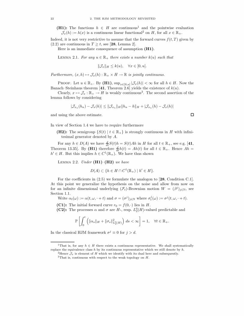
22 2. THE HJM METHODOLOGY REVISITED
(H1): The functions h ∈ H are continuous1 and the pointwise evaluationJx(h) := h(x) is a continuous linear functional2 on H , for all x ∈ R+.
Indeed, it is not very restrictive to assume that the forward curves f(t, T ) given by(2.2) are continuous in T ≥ t, see [28, Lemma 2].
Here is an immediate consequence of assumption (H1).
Lemma 2.1. For any u ∈ R+ there exists a number k(u) such that
‖Jx‖H ≤ k(u), ∀x ∈ [0, u].
Furthermore, (x, h) 7→ Jx(h) : R+ ×H → R is jointly continuous.
Proof. Let u ∈ R+. By (H1), supx∈[0,u] |Jx(h)| <∞ for all h ∈ H . Now theBanach–Steinhaus theorem [41, Theorem 2.6] yields the existence of k(u).
Clearly, x 7→ Jx : R+ → H is weakly continuous3. The second assertion of thelemma follows by considering
|Jxn(hn)− Jx(h)| ≤ ‖Jxn‖H‖hn − h‖H + |Jxn(h)− Jx(h)|
and using the above estimate.
In view of Section 1.4 we have to require furthermore
(H2): The semigroup S(t) | t ∈ R+ is strongly continuous in H with infini-tesimal generator denoted by A.
For any h ∈ D(A) we have ddtS(t)h = S(t)Ah in H for all t ∈ R+, see e.g. [41,
Theorem 13.35]. By (H1) therefore ddth(t) = Ah(t) for all t ∈ R+. Hence Ah =
h′ ∈ H . But this implies h ∈ C1(R+). We have thus shown
Lemma 2.2. Under (H1)–(H2) we have
D(A) ⊂ h ∈ H ∩ C1(R+) | h′ ∈ H.
For the coefficients in (2.5) we formulate the analogon to [28, Condition C.1].At this point we generalize the hypothesis on the noise and allow from now onfor an infinite dimensional underlying (Ft)-Brownian motion W = (βj)j∈N, seeSection 1.1.
Write αt(ω) := α(t, ω, ·+ t) and σ = (σj)j∈N where σjt (ω) := σj(t, ω, ·+ t).
(C1): The initial forward curve r0 = f(0, ·) lies in H .(C2): The processes α and σ are H-, resp. L0
2(H)-valued predictable and
P[∫ t
0
(‖αs‖H + ‖σs‖2L0
2(H)
)ds <∞
]= 1, ∀t ∈ R+.
In the classical HJM framework σj ≡ 0 for j > d.
1That is, for any h ∈ H there exists a continuous representative. We shall systematicallyreplace the equivalence class h by its continuous representative which we still denote by h.
2Hence Jx is element of H which we identify with its dual here and subsequently.3That is, continuous with respect to the weak topology on H.

2.2. THE MUSIELA PARAMETRIZATION 23
Now (2.5) reads, for any t, x ∈ R+,
Jx(rt) = Jx(S(t)r0) +∫ t
0
Jx(S(t− s)αs) ds+∑j∈N
∫ t
0
Jx(S(t− s)σjs) dβjs
= Jx
S(t)r0 +∫ t
0
S(t− s)αs ds+∑j∈N
∫ t
0
S(t− s)σjs dβjs
, P-a.s.
(2.6)
see (1.12). For t fixed, the exceptional P-nullset in equality (2.6) depends on x.But according to (H1) both sides are continuous in x. A standard argument yieldsequality P-a.s. simoultaneously for all x ∈ R+. Pointwise equality of two functionsyields identity of the functions, hence
rt = S(t)r0 +∫ t
0
S(t− s)αs ds+∑j∈N
∫ t
0
S(t− s)σjs dβjs , P-a.s. (2.7)
By [18, Proposition 6.2] the right hand side of (2.7) has a predictable version whichwe still denote by rt. Consequently, r is a mild solution to the stochastic equation
drt = (Art + αt) dt+∑j∈N
σjt dβjt
r0 = f(0, ·).(2.8)
We make an additional assumption.
(C3): There exists a continuous modification of r, still denoted by r.
Condition (C3) is satisfied if S(t) forms a contraction semigroup in H , see [18,Theorem 6.10], or if we require stronger integrability of σ, see [18, Proposition 7.3].Notice, however, that r is not an H-valued semimartingale in general.
Remark 2.3. Combining (C2), (C3) and Lemma 2.1 we conclude that therandom fields rt(ω, x), αt(ω, x) and σjt (ω, x) are P⊗B(R+)-measurable and rt(ω, x)is jointly continuous in (t, x) for P-a.e. ω.
So far we reformulated the classical HJM setup in the spirit of Musiela [37]by putting additional assumptions (C1) and (C2) on the coefficients (reflectingessentially [28, Conditions C.1-C.3]). Moreover, we allow for an infinite dimensionaldriving Brownian motion. The process r, defined as the continuous mild solutionto (2.8), is related to f(t, T ) from (2.2) by
rt(x) = f(t, x+ t) ∀x ∈ R+, P-a.s. ∀t ∈ R+.
From now on, the bond prices and the savings account are given by
P (t, T ) = exp
(−∫ T−t
0
rt(x) dx
), (t, T ) ∈ ∆2
B(t) = exp(∫ t
0
rs(0) ds), t ∈ R+.

24 2. THE HJM METHODOLOGY REVISITED
2.3. Arbitrage Free Term Structure Movements
We derive the dynamics of the discounted bond prices. Since r is not an H-valuedsemimartingale, we cannot use Ito formula directly but we rather have to dealwith the random field (rt(x))t,x∈R+ and apply the stochastic Fubini theorem. Weessentially adapt the technique from [28]. Sufficient conditions for the existenceof an equivalent martingale measure, which ensures the absence of arbitrage, areprovided.
First we introduce the linear functional Iu on H defined by
Iu(h) :=∫ u
0
h(x) dx, u ∈ R+.
There is an immediate consequence of assumption (H1).
Lemma 2.4. The linear functional Iu is continuous on H. In particular,
‖Iu‖H ≤ uk(u), ∀u ∈ R+
where k(u) is the constant from Lemma 2.1.Moreover, the mapping (u, h) 7→ Iu(h) : R+ ×H → R is jointly continuous.
Proof. The estimate is trivial. The second assertion follows as in the proofof Lemma 2.1 by the weak continuity of u 7→ Iu : R+ → H .
It follows from (C3) and Lemma 2.4 that P (t, T ) = exp(−IT−t(rt)) is Ft-measurable and jointly continuous in (t, T ) ∈ ∆2.
Fix (t, T ) ∈ ∆2. Then we have by (2.7), Lemma 2.4 and (1.12)
I := − logP (t, T )
= IT−t(S(t)r0) +∫ t
0
IT−t(S(t− s)αs) ds+∑j∈N
∫ t
0
IT−t(S(t− s)σjs) dβjs
= IT (r0)− It(r0) +∫ t
0
(IT−s(αs)− It−s(αs)) ds
+∑j∈N
∫ t
0
(IT−s(σjs)− It−s(σjs)
)dβjs , P-a.s.
where we took into account the obvious relation IuS(t) = It+u−It. The processes(IT−s(σjs))s∈[0,T ] are predictable and∑
j∈N
∣∣IT−s(σjs(ω))∣∣2 ≤ (Tk(T ))2
∑j∈N‖σjs(ω)‖2H <∞, ∀(s, ω) ∈ [0, T ]× Ω.
Hence (IT−s σs)s∈[0,T ] is `2-valued predictable. Similarly
P
∫ T
0
∑j∈N|IT−s(σjs)|2 ds <∞
= 1,
thus (IT−s σs) ∈ LlocT (R). Replacing T by t, the same holds for (It−s σs)s∈[0,t].
By linearity we can thus split up the integrals and write
I = I1 − I2, P-a.s.

2.3. ARBITRAGE FREE TERM STRUCTURE MOVEMENTS 25
where
I1 := IT (r0) +∫ t
0
IT−s(αs) ds+∑j∈N
∫ t
0
IT−s(σjs) dβjs
I2 := It(r0) +∫ t
0
It−s(αs) ds+∑j∈N
∫ t
0
It−s(σjs) dβjs .
The integrals in I2 need to be transformed. We introduce the mappings
σjs(ω, u) :=
σjs(ω, u− s), if s ≤ u0, otherwise.
Substituting u = x+ s, we have
It−s(σjs) =∫ t−s
0
σjs(x) dx =∫ t
s
σjs(u − s) du =∫ t
0
σjs(u) du.
In view of Remark 2.3, σ = (σj)j∈N is measurable from (R+×Ω×R+,P⊗B(R+))into (`2,B(`2)). Moreover, by Lemma 2.1 and (C2)∫ t
0
∫ t
0
‖σs(u)‖2`2 du ds =∫ t
0
∫ t
0
∑j∈N|σjs(u)|2 du ds
=∫ t
0
∑j∈N
(∫ t−s
0
|σjs(x)|2 dx)ds
≤ t(k(t))2
∫ t
0
∑j∈N‖σjs‖2H ds <∞, P-a.s.
Consequently, the stochastic Fubini theorem 1.12 applies and, by (1.10)–(1.11),
∑j∈N
∫ t
0
It−s(σjs) dβjs =∑j∈N
∫ t
0
(∫ t
0
σjs(u) du)dβjs =
∫ t
0
∑j∈N
∫ t
0
σjs(u) dβjs
du
=∫ t
0
∑j∈N
∫ u
0
σjs(u− s) dβjs
du, P-a.s.
(2.9)
Using the ordinary Fubini theorem we derive similarly∫ t
0
It−s(αs) ds =∫ t
0
(∫ u
0
αs(u − s) ds)du, P-a.s. (2.10)
Combining (2.9) and (2.10) we can write, by (1.12),
I2 =∫ t
0
J0
S(u)r0 +∫ u
0
S(u− s)αs ds+∑j∈N
∫ u
0
S(u− s)σjs dβjs
du
=∫ t
0
ru(0) du, P-a.s.

26 2. THE HJM METHODOLOGY REVISITED
Taking into account IT (r0) = − logP (0, T ) we arrive at the following represen-tation
logP (t, T ) = logP (0, T ) +∫ t
0
(rs(0)− IT−s(αs)) ds
+∑j∈N
∫ t
0
(−IT−s(σjs)) dβjs , P-a.s. ∀(t, T ) ∈ ∆2.
Since P (t, T ) is jointly continuous in (t, T ) ∈ ∆2, the P-nullset can be chosen foreach T ∈ R+ independently of t ∈ [0, T ]. Whence (logP (t, T ))t∈[0,T ] is a contin-uous real-valued semimartingale. Accordingly, so is (logP (t, T ) − logB(t))t∈[0,T ].Applying Ito’s formula to ex gives for the bond price process
P (t, T ) = P (0, T ) +∫ t
0
P (s, T )
rs(0)− IT−s(αs) +12
∑j∈N
(IT−s(σjs))2
ds
+∑j∈N
∫ t
0
P (s, T )(−IT−s(σjs)) dβjs , t ∈ [0, T ]
(2.11)
and for the discounted bond price process Z(t, T ) := P (t,T )B(t)
Z(t, T ) = P (0, T ) +∫ t
0
Z(s, T )
−IT−s(αs) +12
∑j∈N
(IT−s(σjs))2
ds
+∑j∈N
∫ t
0
Z(s, T )(−IT−s(σjs)) dβjs , t ∈ [0, T ].
(2.12)
The following mapping will play an important role. For any continuous functionf on R+ we define the continuous function Sf : R+ → R by
(Sf)(x) := f(x)∫ x
0
f(η) dη, x ∈ R+.
Here is an elementary result on S.
Lemma 2.5. Let Φ = (Φj)j∈N ∈ L02(H). Then f(x) := 1
2
∑j∈N(Ix(Φj))2 is a
continuously differentiable function in x ∈ R+ with
f ′(x) =∑j∈N
(SΦj)(x).
Both series converge uniformly in x on compacts.
Proof. Set fn(x) := 12
∑nj=1(Ix(Φj))2 which is obviously continuously differ-
entiable in x ∈ R+ with
f ′n(x) =n∑j=1
(SΦj)(x).
Moreover, for m < n ∈ N
|fn(x)− fm(x)| + |f ′n(x)− f ′m(x)| ≤ (‖Ix‖2H + ‖Jx‖H‖Ix‖H)n∑
j=m+1
‖Φj‖2H

2.3. ARBITRAGE FREE TERM STRUCTURE MOVEMENTS 27
which tends to zero for m,n→∞ uniformly in x on compacts, by Lemmas 2.1 and2.4. Consequently, the function f(x) = limn→∞ fn(x) exists and is continuouslydifferentiable in x ∈ R+ with f ′(x) = limn→∞ f
′n(x).
Below we will consider a particular Girsanov transformation from P to somerisk neutral measure Q ∼ P on F∞ which only affects a change in the drift α forthe Q-dynamics of r. So let’s pretend for the moment that P itself is a risk neutralmeasure. Then the HJM drift condition [28, (18)] reads as follows.
Lemma 2.6. The discounted bond price process (Z(t, T ))t∈[0,T ] follows a localmartingale for all T ∈ R+ if and only if
α =∑j∈NSσj , dt⊗ dP-a.s. (2.13)
Proof. Let T ∈ R+. By [40, Proposition (1.2)], (Z(t, T ))t∈[0,T ] is a localmartingale if and only if the integral with respect to ds in (2.12) is indistinguishablefrom zero. Since Z(s, T ) > 0, this is equivalent to
IT−t(αt) =12
∑j∈N
(IT−t(σjt ))2, dt⊗ dP-a.s. (2.14)
see the proof of (5.6). The dt ⊗ dP-nullset depends on T . But by Lemma 2.5 theright hand side of (2.14) is continuously differentiable in T ≥ t and so is obviouslythe left hand side. By a standard argument we find a dt⊗ dP-nullset N ∈ P withthe property that
Ix(αt(ω)) =12
∑j∈N
(Ix(σjt (ω)))2, ∀(t, ω, x) ∈ N c × R+.
Differentiation yields the assertion.
Observe that Lemma 2.6 imposes through (2.13) implicitly a measurability andintegrability condition on
∑j∈N Sσj . Their validity is guaranteed by the following
pair of assumptions.(C4): The processes Sσj are H-valued predictable.(H3): There exists a constant K such that
‖Sh‖H ≤ K‖h‖2Hfor all h ∈ H with Sh ∈ H .
In general, P is considered as physical measure. Accordingly, the conditions ofLemma 2.6 are not satisfied under P.
Definition 2.7. We call a measure Q on F∞ an equivalent local martingalemeasure (ELMM) if
i) Q ∼ P on F∞ii) (Z(t, T ))t∈[0,T ] is a Q-local martingale for all T ∈ R+.
The next condition assures the existence of an ELMM, see [28, Condition C.4].(C5): There exists an `2-valued predictable process γ = (γj)j∈N satisfying
Novikov’s condition (1.14) and∑j∈N
γjσj =∑j∈NSσj − α, dt⊗ dP-a.s. (2.15)

28 2. THE HJM METHODOLOGY REVISITED
By Holder’s inequality and Lemma 2.1, the series
Jx
∑j∈N
γjt σjt
=∑j∈N
γjtJx(σjt )
converges uniformly in x on compacts. Taking into account Lemma 2.5 and inte-grating, we see that (2.15) is equivalent to∑j∈N
γjt IT−t(σjt ) =
12
∑j∈N
(IT−t(σjt )
)2
− IT−t(αt), ∀T ≥ t, dt⊗ dP-a.s. (2.16)
There is an intuitive interpretation of −γ as market price of risk , by consideringthe bond price dynamics (2.11): after localization, the right hand side of (2.16) is,roughly speaking, the difference between the “average return E
[dP (t,T )P (t,T )
]” of the
bond and the “risk-less rate” rt(0). Whence the interpretation of −γjt as marketprice of risk in units of the volatility, −IT−t(σjt ), for the j-th noise factor. Whencealso the expression risk neutral measure for Q.
Condition (C5) allows for Lemma 1.14. Hence we can define Q ∼ P on F∞ bydQdP
= E(γ ·W )∞,
recall the definition of the stochastic exponential (1.13). Girsanov’s theorem, seeProposition 1.16, yields that
Wt = Wt −∫ t
0
γs ds, t ∈ R+
is a Wiener process for the measure Q. The dynamics of r change accordingly.
Proposition 2.8. Under the above assumptions, r satisfies
rt = S(t)r0 +∫ t
0
S(t− s)∑j∈NSσjs
ds+∑j∈N
∫ t
0
S(t− s)σjs dβjs (2.17)
with respect to Q. Consequently, Q is an ELMM.
Proof. The statement on (rt) follows by combining (1.15), (2.7) and (2.15).Lemma 2.6 yields the assertion on Q.
2.4. Contingent Claim Valuation
This section sketches how to value contingent claims in the preceding bond mar-ket. Yet we do not address here the question of completeness, which essentially isequivalent to uniqueness of the ELMM Q. Since the underlying noise is an infinitedimensional Brownian motion, the notion of infinite dimensional admissible tradingstrategies were convenient. This, however, is beyond the scope of this thesis andwill be exploited elsewhere. For a treatment of the finite dimensional case we referthe reader to [38, Section 10.1]. Measure-valued trading strategies are introducedin [9].
We content ourself in postulating that Q is the risk neutral measure4 andall prices are computed as expectations under Q. This is justified at least if alldiscounted bond price processes (Z(t, T ))t∈[0,T ] follow true Q-martingales. Since
4Equivalently, −γ is the market price of risk.

2.4. CONTINGENT CLAIM VALUATION 29
then any attainable claim5 will admit a unique arbitrage price. It is determined bythe replicating strategy.
The subsequent introduction of the forward measure, the forward LIBOR ratesand caplets is preliminary for the discussion of the popular BGM model in Sec-tion 3.6.
2.4.1. When Is the Discounted Bond Price Process a Q-Martingale?We can give a sufficient condition for the discounted bond price process to follow atrue Q-martingale. The dynamics (2.12) read under Q
Z(t, T ) = P (0, T ) +∑j∈N
∫ t
0
Z(s, T )(−IT−s(σjs)) dβjs , t ∈ [0, T ],
see (2.16). Ito’s formula yields the representation as the stochastic exponential
Z(t, T ) = P (0, T ) E
∑j∈N
∫ ·0
(−IT−s(σjs)) dβjs
t
. (2.18)
But now we can use Novikov’s criterion, see Lemma 1.14, to derive
Lemma 2.9. If
EQ
[exp
(12
∫ T
0
‖IT−t σt‖2`2 dt)]
<∞
then (Z(t, T ))t∈[0,T ] is a Q-martingale.
Another sufficient criterion is positivity of the forward rates. Indeed, if rt ≥ 0for all t ∈ [0, T ] then 0 ≤ Z(t, T ) ≤ 1 for all t ∈ [0, T ]. Moreover, a boundedlocal martingale is a uniformly integrable martingale. Positivity of r is relatedto stochastic invariance of the positive cone of functions h ≥ 0 in H under thedynamics (2.8). We do not address this problem here and refer the reader to [34].
2.4.2. The Forward Measure. For pricing purposes it is convenient to usea technique called “change of numeraire”, see [20] for a thorough treatment. Wegive an application for pricing bond options.
Assume that (Z(t, T ))t∈[0,T ] is a Q-martingale. We can define the measureQT ∼ Q on (Ω,FT ) by dQT
dQ = 1P (0,T )B(T ) . By (2.18) we then have
EQ[dQT
dQ| Ft
]=Z(t, T )P (0, T )
= E
∑j∈N
∫ ·0
(−IT−s(σjs)) dβjs
t
, t ∈ [0, T ]. (2.19)
Definition 2.10. The measure QT is called the T -forward measure.
A claim X due at time T is in L1(Ω,FT ,QT ) if and only if XB(T ) ∈ L1(Ω,FT ,Q).
Bayes’ rule, see e.g. [32, Lemma 5.3, Chapter 3], yields the equality
P (t, T )EQT [X | Ft] = B(t)EQ[
X
B(T )| Ft
], Q-a.s. ∀t ∈ [0, T ]. (2.20)
On the right hand side stands the time t price of the claim X . This is a very usefulrelation, since the left hand side allows for closed form expressions if X has a nicedistribution under QT . We will later use it for pricing a cap.
5if ever defined in a reasonable way

30 2. THE HJM METHODOLOGY REVISITED
2.4.3. Forward LIBOR Rates. Let’s introduce an important QT -local mar-tingale. We will use the notation Ivu := Iv − Iu for (u, v) ∈ ∆. Fix δ > 0.
Definition 2.11. The forward δ-period6 LIBOR rate for the future date Tprevailing at time t is
L(t, T ) :=1δ
(eI
T+δ−tT−t (rt) − 1
), (t, T ) ∈ ∆2.
We can re-express L(t, T ) directly in term of bond prices
1 + δL(t, T ) =P (t, T )
P (t, T + δ).
Whence the meaning of L(t, T ) as forward average simple rate for a loan over thefuture time period [T, T + δ].
Let T ∈ R+ and write `(t, T ) := IT+δ−tT−t (rt). Combining Lemma 2.4 and (2.17)
we conclude that (`(t, T ))t∈[0,T ] is a real-valued continuous semimartingale and
`(t, T ) = `(0, T ) +∫ t
0
IT+δ−tT−t
S(t− s)∑j∈NSσjs
ds
+∑j∈N
∫ t
0
IT+δ−tT−t
(S(t− s)σjs
)dβjs
= `(0, T ) +12
∫ t
0
∑j∈N
((IT+δ−s(σjs))
2 − (IT−s(σjs))2)ds
+∑j∈N
∫ t
0
IT+δ−sT−s (σjs) dβ
js , t ∈ [0, T ].
We have used the relation IT+δ−tT−t S(t−s) = IT+δ−s
T−s and Lemma 2.5. Ito’s formulayields
L(t, T ) = L(0, T )
+12δ
∫ t
0
e`(s,T )∑j∈N
((IT+δ−s(σjs))
2 − (IT−s(σjs))2 + (IT+δ−sT−s (σjs))
2)ds
+∑j∈N
1δ
∫ t
0
e`(s,T )IT+δ−sT−s (σjs) dβ
js
= L(0, T ) +1δ
∫ t
0
e`(s,T )∑j∈N
(IT+δ−sT−s (σjs) IT+δ−s(σjs)
)ds
+∑j∈N
1δ
∫ t
0
e`(s,T )IT+δ−sT−s (σjs) dβ
js , t ∈ [0, T ].
Now assume that (Z(t, T + δ))t∈[0,T+δ] is a Q-martingale. Using (2.19) andGirsanov’s theorem 1.15 we conclude that
β(T+δ),jt = βjt +
∫ t
0
IT+δ−s(σjs) ds, t ∈ [0, T + δ], j ∈ N
6Typically, δ stands for 3 or 6 months.

2.4. CONTINGENT CLAIM VALUATION 31
are independent (Ft)t∈[0,T+δ]-Brownian motions under QT+δ. Consequently, theprocess (L(t, T ))t∈[0,T ] is a QT+δ-local martingale with representation
L(t, T ) = L(0, T ) +∑j∈N
1δ
∫ t
0
e`(s,T )IT+δ−sT−s (σjs) dβ
(T+δ),js , t ∈ [0, T ]. (2.21)
2.4.4. Caps. For a thorough introduction to interest rate derivatives, such asswaps, caps, floors and swaptions, we refer to [38, Chapter 16]. We restrict ourconsideration to the following basic instrument.
A caplet with reset date T and settlement date T + δ pays the holder thedifference between the LIBOR L(T, T ) and the strike rate κ. It’s cash-flow at timeT + δ is
δ(L(T, T )− κ)+.
A cap is a strip of caplets. If we can price caplets, we can price caps. The arbitrageprice of the caplet at time t ≤ T equals, see [38, p. 391],
Cpl(t) = B(t)EQ[
1B(T + δ)
δ(L(T, T )− κ)+ | Ft]
= P (t, T + δ)EQT+δ
[δ(L(T, T )− κ)+ | Ft
],
where we have used (2.20).Suppose there exists a deterministic `2-valued measurable function π(·, T ) =
(πj(·, T ))j∈N with∫ T
0‖π(t, T )‖2`2 dt <∞ and such that
IT+δ−tT−t (σjt ) = (1− e−`(t,T ))πj(t, T ), dt⊗ dQ-a.s. on [0, T ]× Ω. (2.22)
Then (2.21) reads
L(t, T ) = L(0, T ) +∑j∈N
∫ t
0
L(s, T )πj(s, T ) dβ(T+δ),js , t ∈ [0, T ].
This equation is uniquely solved by the stochastic exponential
L(t, T ) = L(0, T )E
∑j∈N
∫ ·0
πj(s, T ) dβ(T+δ),js
t
.
By [18, Lemma 10.15] there exists a real-valued standard (Ft)t∈[0,T ]-Brownian mo-tion (β0
t )t∈[0,T ] under QT+δ such that∑j∈N
∫ t
0
πj(s, T ) dβ(T+δ),js =
∫ t
0
‖π(s, T )‖2`2 dβ0s , t ∈ [0, T ].
Accordingly, L(T, T ) is lognormally distributed under QT+δ, and the following pric-ing formula holds, see [38, Lemma 16.3.1].
Lemma 2.12. Under the above assumptions, the time t price of the caplet equals
Cpl(t) = δP (t, T + δ) (L(t, T )N(e1(t, T ))− κN(e2(t, T ))) (2.23)

32 2. THE HJM METHODOLOGY REVISITED
where
e1,2 :=log(L(t,T )κ
)± 1
2v20(t, T )
v0(t, T )
v20(t, T ) :=
∫ T
t
‖π(s, T )‖2`2 ds.
and N stands for the standard Gaussian cumulative distribution function.
BGM [12] present a method for modelling the forward LIBOR rates such that(2.22) holds for all T ∈ R+. We will recapture their approach in the present settingin Section 3.6.
A Summary of Conditions
For the reader’s convenience we summarize the conditions made so far. Recall thedefinition of S
(Sf)(x) := f(x)∫ x
0
f(η) dη, x ∈ R+
for any continuous function f : R+ → R.(H1): The functions h ∈ H are continuous, and the pointwise evaluationJx(h) := h(x) is a continuous linear functional on H , for all x ∈ R+.
(H2): The semigroup S(t) | t ∈ R+ is strongly continuous in H with infini-tesimal generator denoted by A.
(H3): There exists a constant K such that
‖Sh‖H ≤ K‖h‖2Hfor all h ∈ H with Sh ∈ H .
(C1): The initial forward curve r0 = f(0, ·) lies in H .(C2): The processes α and σ are H-, resp. L0
2(H)-valued predictable and
P[∫ t
0
(‖αs‖H + ‖σs‖2L0
2(H)
)ds <∞
]= 1, ∀t ∈ R+.
(C3): There exists a continuous modification of r, still denoted by r.(C4): The processes Sσj are H-valued predictable.(C5): There exists an `2-valued predictable process γ = (γj)j∈N satisfying
Novikov’s condition (1.14) and∑j∈N
γjσj =∑j∈NSσj − α, dt⊗ dP-a.s. (2.24)
2.5. What Is a Model?
Up to now we analyzed the stochastic behavior of a single generic forward curveprocess r within the HJM framework. For modelling purposes we rather wantthe stochastic evolution being described by a dynamical system like (2.8) withstate dependent coefficients αt(ω) = α(t, ω, rt(ω)) and σt(ω) = σ(t, ω, rt(ω)), whichallows for arbitrary initial curves r0.
From the last section it seems plausible to specify as model ingredients thevolatility structure σ and a market price of risk vector −γ. We then let the driftα being defined by (2.24). Proposition 2.8, accordingly, assures the existence of anELMM Q.

2.5. WHAT IS A MODEL? 33
As it can be seen from (2.17), γ does not appear in the Q-dynamics of r. Thus,instead of solving (2.8) directly we rather start with the Wiener process W underQ, solve (2.17) and transform W W , by Girsanov’s theorem, to have γ backin the drift for the P-dynamics of r. Compare with [28, Lemma 1]. That way,however, the measure P and the Wiener process W will depend on r implicitly byγt(ω) = γ(t, ω, rt(ω)). Yet W will be adapted to (Ft). Which is convenient sincewe never needed the filtration (Ft) being generated by W .
Henceforth we are given a complete filtered probability space
(Ω,F , (Ft)t∈R+ ,Q)
satisfying the usual assumptions, the measureQ being considered as the risk neutralmeasure. Let W = (βj)j∈N be an infinite dimensional (Ft)-Brownian motion underQ. The random mappings σ(t, ω, h) (volatility structure) and −γ(t, ω, h) (marketprice of risk) are specified in accordance with the following assumptions.
(D1): The mappings σ and γ are measurable from (R+ × Ω × H,P ⊗ B(H))into (L0
2(H),B(L02(H))), resp. (`2,B(`2)).
(D2): The mappings Sσj are measurable from (R+ × Ω × H,P ⊗ B(H)) into(H,B(H)).
(D3): There exists a function Γ ∈ L2(R+) such that
‖γ(t, ω, h)‖`2 ≤ Γ(t), ∀(t, ω, h) ∈ R+ × Ω×H.Observe that assumptions (D1)–(D2) together with (H3) imply that
∑j∈N Sσj
is a measurable mapping from (R+ × Ω×H,P ⊗ B(H)) into (H,B(H)).
Definition 2.13. By the HJMM equation (HJM equation in the Musiela para-metrization) we mean the following stochastic equation7 in H
drt = (Art + FHJM (t, rt)) dt+ σ(t, rt) dWt
r0 = h0
(2.25)
where FHJM (t, ω, h) :=∑j∈N Sσj(t, ω, h).
Definition 2.14. Let σ, γ satisfy (D1)–(D3) and let I ⊂ H be a set of initialforward curves. We call (σ, γ, I) a (local) HJM model in H if for every space timeinitial point (t0, h0) ∈ R+× I there exists a unique continuous (local) mild solutionr = r(t0,h0) to the time t0-shifted 8 HJMM equation (2.25).
This definition is justified by the following result.
Theorem 2.15. Let (σ, γ, I) be an HJM model. Then any space time initialpoint (t0, h0) ∈ R+ × I specifies a measure P ∼ Q on F∞ and a Wiener process Wwith respect to (Ω,F∞, (F (t0)
t )t∈R+ ,P) such that (C1)–(C5) hold for
αt(ω) = FHJM (t0 + t, ω, rt(ω))−∑j∈N
γj(t0 + t, ω, rt(ω))σj(t0 + t, ω, rt(ω))
σt(ω) = σ(t0 + t, ω, rt(ω))
γt(ω) = γ(t0 + t, ω, rt(ω))
where r = r(t0,h0). Accordingly, Q is an ELMM for this setup.
7See Remark 1.18 for notation.8recall (1.18)
34 2. THE HJM METHODOLOGY REVISITED
Proof. Let r = r(t0,h0) be the continuous mild solution to the time t0-shiftedversion of (2.25). From (D3) we deduce that∫
R+
‖ − γ(t0 + s, ω, rs(ω))‖2`2 ds ≤ ‖Γ‖2L2(R+) <∞, ∀ω ∈ Ω. (2.26)
Hence Lemma 1.14 applies and we can define the measure P ∼ Q on F∞ = F (t0)∞
bydPdQ
= E(−γ · W (t0))∞. (2.27)
According to Girsanov’s theorem, see Proposition 1.16,
Wt = W(t0)t +
∫ t
0
γs ds
is a Wiener process under P.By (H3) and Holder’s inequality
‖αt‖H ≤ K∑j∈N‖σjt ‖2H + ‖γt‖`2‖σt‖L0
2(H) ≤ (K +12
)‖σt‖2L02(H) +
12‖γt‖2`2 .
Now (2.26) yields (C2), since (σt)t∈R+ ∈ Lloc(H) by the very definition of a mildsolution. Using (1.15), the process r is seen to be the continuous mild solution of(2.8) with f(0, ·) replaced by h0, whence (C3). Conditions (C4)–(C5) are impliedby (D1)–(D3) and, clearly, Q is an ELMM for this setup.
Remark 2.16. Theorem 2.15 points out that a mild solution r to the HJMMequation (2.25) is the right concept for the HJM framework. This is also in accor-dance with Remark 1.25. It is therefore an essential request to derive the resultsfrom [7] without assuming that r is a (local) strong solution, see [7, Assumption 2.1]
Remark 2.17. Local HJM models are useless for pricing financial instruments.Yet in some cases we only can assert local existence and uniqueness for the HJMMequation (2.25), which is still adapted for the consistency analysis in Chapter 4.Therefore we also included the local case in Definition 2.14.
The specification of the initial forward curve set I is convenient and allowsto incorporate also the following classical examples in our framework. Let −γ beany market price of risk satisfying (D1) and (D3). See Sections 4.4.1–4.4.2 forterminology and results.
Example 2.18 (CIR Model). Here I = g0 + yg1 | y > 0 where g0, g1 aregiven functions, σ1 = σ1(h) =
√αJ0(h)g1 for all h ∈ I and σj ≡ 0 for j ≥ 2.
Then (σ, γ, I) is a local HJM model.
Example 2.19 (Vasicek Model). The volatility is constant, σ1 ≡√ag1, where
g1(x) = eβx and σj ≡ 0 for j ≥ 2. Moreover, I = g0 + yg1 | y ∈ R and g0 is agiven function. Then (σ, γ, I) is an HJM model.
It is desirable to find easy verifiable criterions for σ to provide a (local) HJMmodel. We will approach this by the classical Lipschitz condition, see Section 1.4.2.But if σ(t, ω, h) is (locally) Lipschitz continuous in h, what about FHJM (t, ω, h)?In the next chapter we present a Hilbert space of forward curves which is both eco-nomically reasonable and convenient for deriving (local) existence and uniquenessresults for the HJMM equation (2.25).

CHAPTER 3
The Forward Curve Spaces Hw
3.1. Definition of Hw
We introduce a class of Hilbert spaces satisfying (H1)–(H3)1 and which are co-herent with economical reasoning about the forward curve x 7→ rt(x).
Since in practice the forward curve is obtained by smoothing data points usingsmooth fitting methods, see Chapters 5 and 6, it is reasonable to assume∫
R+
|r′t(x)|2 dx <∞.
Moreover, the curve flattens for large time to maturity x. There is no reason tobelieve that the forward rate for an instantaneous loan that begins in 10 yearsdiffers much from one which begins one day later. We take this into account bypenalizing irregularities of rt(x) for large x by some increasing weighting functionw(x) ≥ 1, that is, ∫
R+
|r′t(x)|2 w(x)dx <∞.
However, this does not define a norm yet since constant functions are not distin-guished. So we add the square of the short rate |rt(0)|2.
We shall give a mathematically correct approach. Recall the fact that if h ∈L1
loc(R+) possesses a weak derivative2 h′ ∈ L1loc(R+), then there exists an absolutely
continuous representative of h, still denoted by h, such that
h(x)− h(y) =∫ x
y
h′(u) du, ∀x, y ∈ R+. (3.1)
This can be found e.g. in [14, Section VIII.2]. Accordingly, the following definitionmakes sense.
Definition 3.1. Let w : R+ → [1,∞) be a non-decreasing C1-function suchthat
w−13 ∈ L1(R+). (3.2)
We write
‖h‖2w := |h(0)|2 +∫R+
|h′(x)|2 w(x)dx
and define
Hw :=h ∈ L1
loc(R+) | ∃h′ ∈ L1loc(R+) and ‖h‖w <∞
.
The choice of Hw is established by the next theorem.
1see page 322uniquely specified by
∫R+
h(x)ϕ′(x) dx = −∫R+
h′(x)ϕ(x) dx for all ϕ ∈ C1c ((0,∞))
35

36 3. THE FORWARD CURVE SPACES Hw
Theorem 3.2. The set Hw equipped with ‖ ·‖w forms a separable Hilbert spacemeeting (H1)–(H3).
Before proving the theorem we give two guiding examples of admissible weight-ing functions w which satisfy condition (3.2).
Example 3.3. w(x) = eαx, for α > 0.
Example 3.4. w(x) = (1 + x)α, for α > 3.
Proof. It is clear that ‖ · ‖w is a norm. Consider the separable Hilbert space
R×L2(R+) equipped with the norm(| · |2 + ‖ · ‖2L2(R+)
) 12. Then the linear operator
T : Hw → R× L2(R+) given by
Th =(h(0), h′w
12
), h ∈ Hw
is an isometry with inverse
(T−1(u, f))(x) = u+∫ x
0
f(η)w−12 (η) dη, (u, f) ∈ R× L2(R+).
Hence Hw is a separable Hilbert space.
We claim that
D0 := f ∈ C2(R+) | f ′ ∈ C1c (R+)
is dense in Hw. Indeed, C1c (R+) is dense in L2(R+), see [14, Corollaire IV.23].
Fix h ∈ Hw and let (fn) be a approximating sequence of h′w12 in L2(R+) with
fn ∈ C1c (R+) for all n ∈ N. Write hn := T−1(h(0), fn). Obviously, hn ∈ D0 and
hn → h in Hw. Whence the claim.
Since w−1 is bounded, (3.2) implies in particular w−1 ∈ L1(R+). The subse-quent Sobolev-type inequalities (3.4)–(3.8) are crucial. Throughout, h denotes afunction in Hw. The constants C1–C4 are universal and depend only on w.
First we prove
‖h′‖L1(R+) ≤ C1‖h‖w. (3.3)
This is established by Holder’s inequality∫R+
|h′(x)| dx =∫R+
|h′(x)|w 12 (x)w−
12 (x) dx
≤(∫
R+
|h′(x)|2 w(x)dx
) 12(∫
R+
w−1(x) dx
) 12
≤ ‖h‖w ‖w−1‖12L1(R+).
An important consequence of (3.3) is that h(x) converges to a limit h(∞) ∈ Rfor x→∞, see (3.1). This is of course a desirable property for forward curves.
For C2 = 1 + C1 it follows easily from (3.1) and (3.3) that
‖h‖L∞(R+) ≤ C2‖h‖w. (3.4)
Write Π(x) :=∫∞xw−1(η) dη. Then we have, by monotonicity of w,
Π(x) ≤ w− 23 (x)
∫ ∞x
w−13 (η) dη ≤ w− 2
3 (x)‖w− 13 ‖L1(R+), x ∈ R+

3.1. DEFINITION OF Hw 37
and hence, by (3.2),
‖Π 32w‖L∞(R+) ≤ ‖w−
13 ‖L1(R+) <∞. (3.5)
Moreover,
‖Π 12 ‖L1(R+) ≤ ‖w−
13 ‖2L1(R+) <∞. (3.6)
By the same method as above we derive∫R+
|h(x) − h(∞)| dx =∫R+
∣∣∣ ∫ ∞x
h′(η)w12 (η)w−
12 (η) dη
∣∣∣ dx≤∫R+
(∫ ∞x
|h′(η)|2 w(η)dη) 1
2
Π12 (x) dx
≤ ‖h‖w ‖Π12 ‖L1(R+).
Hence, by (3.6),
‖h− h(∞)‖L1(R+) ≤ C3‖h‖w. (3.7)
Finally we compute, using Holder’s inequality again,∫R+
|h(x) − h(∞)|4 w(x)dx =∫R+
∣∣∣ ∫ ∞x
h′(η)w12 (η)w−
12 (η) dη
∣∣∣4 w(x)dx
≤∫R+
(∫R+
|h′(η)|2 w(η)dη
)2
Π2(x)w(x)dx
≤ ‖h‖4w ‖Π32w‖L∞(R+) ‖Π
12 ‖L1(R+).
Therefore, by (3.5)–(3.6),
‖(h− h(∞))4w‖L1(R+) ≤ C4‖h‖4w. (3.8)
Now we can prove (H1)–(H3). Estimate (3.4) yields continuity of the linearfunctional Jx for all x ∈ R+. Since by the preceding remarks, see (3.1), Hw consistsof continuous functions, (H1) is established.
Let h ∈ Hw and ϕ ∈ C1c ((0,∞)). Then the shift semigroup S(t) satisfies∫
R+
S(t)h(x)ϕ′(x) dx =∫R+
h(x)ϕ′(x− t) dx = −∫R+
h′(x)ϕ(x − t) dx
= −∫R+
h′(x+ t)ϕ(x) dx(3.9)
since ϕ(· − t) ∈ C1c ((t,∞)). Consequently, (S(t)h)′ exists and equals S(t)h′. In
view of (3.4) it follows
‖S(t)h‖2w = |h(t)|2 +∫R+
|h′(x+ t)|2 w(x)dx ≤ (C22 + 1)‖h‖2w. (3.10)
We have used the monotonicity of w. Hence S(t)h ∈ Hw and S(t) is bounded forall t ∈ R+.

38 3. THE FORWARD CURVE SPACES Hw
We have to show strong continuity of S(t). We start with the following obser-vation. By (3.1)
h(x+ t)− h(x) = t
∫ 1
0
h′(x + st) ds, h ∈ Hw. (3.11)
Let g ∈ D0. Since g′ ∈ Hw, (3.10) and (3.11) yield
‖S(t)g − g‖2w = |g(t)− g(0)|2 +∫R+
|g′(x + t)− g′(x)|2 w(x)dx
≤ |g(t)− g(0)|2 + t2∫ 1
0
∫R+
|g′′(x+ st)|2w(x) dx ds
≤ |g(t)− g(0)|2 + t2∫ 1
0
‖S(st)g′‖2w ds→ 0 for t→ 0.
Hence S(t) is strongly continuous on D0. But for any h ∈ Hw and ε > 0 thereexists g ∈ D0 with ‖h− g‖w ≤ ε
4(C2+1) . Combining this with (3.10) yields
‖S(t)h− h‖w ≤ ‖S(t)(h− g)‖w + ‖S(t)g − g‖w + ‖g − h‖w≤ (C2 + 1)
ε
4(C2 + 1)+ ‖S(t)g − g‖w +
ε
4(C2 + 1)≤ ε
for t small enough. We conclude that S(t) is strongly continuous on Hw, whencethe validity of (H2).
It remains to prove the estimate in (H3). Let h ∈ Hw. Similarly to (3.9) oneshows that (Sh)′ exists with
(Sh)′(x) = h′(x)∫ x
0
h(η) dη + h2(x).
We define
H0w := h ∈ Hw | h(∞) = 0. (3.12)
By (3.4), H0w is a closed subspace of Hw. We claim that
Sh ∈ Hw ⇐⇒ h ∈ H0w. (3.13)
Assume that h(∞) > 0. Then there exists x0 ∈ R+ such that h(x) ≥ h(∞)2 for all
x ≥ x0. But then
Sh(x) ≥ h(x)∫ x0
0
h(η) dη +(h(∞)
2
)2
(x − x0), ∀x ≥ x0
which explodes for x → ∞. The same reasoning applies if h(∞) < 0. Whence thenecessity in (3.13).
Conversely, assume that h(∞) = 0. Using (3.7) and (3.8) we estimate
‖Sh‖2w =∫R+
∣∣∣h′(x)∫ x
0
h(η) dη + h2(x)∣∣∣2 w(x)dx
≤ 2∫R+
|h′(x)|2
(∫ x
0
|h(η)| dη)2
+ h4(x)
w(x)dx
≤ 2(‖h‖2L1(R+) ‖h‖2w + C4‖h‖4w) ≤ 2(C23 + C4)‖h‖4w.
Hence Sh ∈ Hw and (3.13) is proved. Moreover, we conclude that (H3) holds withK =
√2(C2
3 + C4).

3.1. DEFINITION OF Hw 39
Remark 3.5. It is not difficult to see that (H1) and (H2) hold without as-sumption (3.2). Yet it makes the proof more handy.
The preceding proof allows for identifying the full generator A of S(t) in Hw.
Corollary 3.6. We have D(A) = h ∈ Hw | h′ ∈ Hw and Ah = h′.
Proof. Write D := h ∈ Hw | h′ ∈ Hw. By Lemma 2.2, D(A) ⊂ D.Conversely, let h ∈ D. Applying (3.11) we get
h′(x+ t)− h′(x)t
− h′′(x) =∫ 1
0
(h′′(x + st)− h′′(x)) ds.
Consequently,
n(t) :=∫R+
∣∣∣h′(x + t)− h′(x)t
− h′′(x)∣∣∣2 w(x)dx
≤∫ 1
0
∫R+
|h′′(x+ st)− h′′(x)|2 w(x)dx ds
≤∫ 1
0
‖S(st)h′ − h′‖2w ds→ 0 for t→ 0
by dominated convergence, see (3.10). Since h′ is continuous on R+, see (3.1), weconclude∥∥∥S(t)h− h
t− h′
∥∥∥2
w=∣∣∣h(t)− h(0)
t− h′(0)
∣∣∣2 + n(t)→ 0 for t→ 0,
whence h ∈ D(A).
Most important for the HJMM equation is the following result.
Corollary 3.7. The mapping S : H0w → H0
w is locally Lipschitz continuous,that is
‖Sg − Sh‖w ≤ C5(‖g‖w + ‖h‖w) ‖g − h‖w, ∀g, h ∈ H0w
where the constant C5 only depends on w.
Proof. In view of (3.13) and (3.7) it’s immediate that Sh ∈ H0w for all h ∈ H0
w.Let g, h ∈ H0
w. Using Holder’s inequality and (3.7)–(3.8) we calculate
‖Sg − Sh‖2w =∫R+
∣∣∣g′(x)∫ x
0
g(η) dη − h′(x)∫ x
0
h(η) dη + g2(x) − h2(x)∣∣∣2 w(x)dx
≤ 3∫R+
|g′(x)|2∣∣∣ ∫ x
0
(g(η)− h(η)) dη∣∣∣2 w(x)dx
+ 3∫R+
∣∣∣ ∫ x
0
h(η) dη∣∣∣2|g′(x) − h′(x)|2 w(x)dx
+ 3∫R+
(g(x) + h(x))2w12 (x)(g(x) − h(x))2w
12 (x) dx
≤ 3(‖g‖2w ‖g − h‖2L1(R+) + ‖h‖2L1(R+) ‖g − h‖2w
)+ 3 ‖(g + h)4w‖
12L1(R+) ‖(g − h)4w‖
12L1(R+)
≤ 3(C23 + 2C4)(‖g‖2w + ‖h‖2w) ‖g − h‖2w

40 3. THE FORWARD CURVE SPACES Hw
and we have used the universal inequality
|x1 + · · ·+ xk|2 ≤ k(|x1|2 + · · ·+ |xk|2
), k ∈ N. (3.14)
Setting C5 =√
3(C23 + 2C4) yields the result.
3.2. Volatility Specification
Working in the space Hw we can give simple criteria for σ(t, ω, h) to provide a(local) HJM model.
Condition (D2) and (3.13) clearly force σj ∈ H0w, recall (3.12). This is of
course a desirable property since we don’t want the forward rates rt(x) being toovolatile for large x, see (2.6). In fact, Corollary 3.7 yields
Lemma 3.8. Let σ meet (D1) with H = Hw and L02(H) replaced by L0
2(H0w).
Then (D2) is satisfied as well.
From now on we require that σ satisfies the assumptions of Lemma 3.8. Inview of Corollary 1.24 it’s enough to require local Lipschitz continuity of σ(t, ω, h)and FHJM (t, ω, h) in h for asserting local existence and uniqueness for the HJMMequation (2.25). The choice of Hw gains in interest if we consider the followingproperty.
Let σ(t, ω, h) be locally Lipschitz continuous in h with Lipschitz constant C =C(R) and suppose
‖σ(t, ω, 0)‖L02(Hw) ≤ C, ∀(t, ω) ∈ R+ × Ω (3.15)
for a constant C. This clearly gives
‖σ(t, ω, h)‖L02(Hw) ≤ C + C(R)R, ∀h ∈ BR(Hw), ∀R ∈ R+. (3.16)
Whence σ is locally bounded.
Lemma 3.9. i) Let σ satisfy the above assumptions. Then FHJM (t, ω, h) islocally Lipschitz continuous in h.
ii) Suppose in addition that σ(t, ω, h) is Lipschitz continuous in h and uniformlybounded:
‖σ(t, ω, h)‖L02(Hw) ≤ C, ∀(t, ω, h) ∈ R+ × Ω×Hw, (3.17)
for some constant C. Then the same holds true for FHJM (t, ω, h).
Proof. For simplicity of notation we abandon temporarily the (t, ω)-depen-dence of σ and FHJM .
Let h1, h2 ∈ BR(Hw) and write ∆ := ‖FHJM (h1) − FHJM (h2)‖w. By Corol-lary 3.7 and Holder’s inequality
∆ ≤∑j∈N‖Sσj(h1)− Sσj(h2)‖w
≤ C5
∑j∈N
(‖σj(h1)‖w + ‖σj(h2)‖w
)‖σj(h1)− σj(h2)‖w
≤ C5
(‖σ(h1)‖L0
2(Hw) + ‖σ(h2)‖L02(Hw)
)‖σ(h1)− σ(h2)‖L0
2(Hw)
≤ C5C(R)(‖σ(h1)‖L0
2(Hw) + ‖σ(h2)‖L02(Hw)
)‖h1 − h2‖w.
Combining this with (3.16) proves i) and the first part of ii). The boundednessassertion on FHJM is a consequence of (H3).

3.3. THE YIELD CURVE 41
Combining Lemmas 3.8–3.9 with Theorem 1.23 and Corollary 1.24 we get ourmain existence and uniqueness result for the HJMM equation. Denote by −γ amarket price of risk vector meeting (D1) and (D3).
Theorem 3.10. i) Let σ be as in Lemma 3.9.i). Then (σ, γ,Hw) is a localHJM model in Hw.
ii) Let σ be as in Lemma 3.9.ii). Then (σ, γ,Hw) is an HJM model in Hw andall discounted bond price processes (Z(t, T ))t∈[0,T ] are true Q-martingales.Moreover, any mild solution r(t0,h0) of the time t0-shifted HJMM equation(2.25) is also a weak solution, (t0, h0) ∈ R+ ×Hw.
Proof. Only the statement on (Z(t, T ))t∈[0,T ] remains to be proved. But thisis a straightforward consequence of Lemma 2.9 and the estimate
‖IT−t σ(t, rt)‖2`2 ≤ (Tk(T ))2‖σ(t, rt)‖2L02(Hw) ≤ (Tk(T ))2C2,
see Lemma 2.4.
We shall examine three types of possible volatility specifications. The first onecorresponds to the classical HJM framework where the volatility depends locally onthe state variable. It turns out that in this case one merely gets local HJM models.For example the one which is presented in [28, Section 7].
The second type is much more convenient. Here the volatility depends on afunctional value of the state variable. It is easy to find sufficient conditions forproviding an HJM model in this case.
Lastly, we recapture the BGM [12] model which we already mentioned in Sec-tion 2.4.4. However, since also this type of volatility is of local nature, we merelyget a local HJM model.
Subsequently, there follows an intermediary section where we introduce an im-portant financial variable.
3.3. The Yield Curve
We already know by Riesz representation theorem that the functionals Jx and Ixcan be identified with elements in Hw, see Theorem 3.2 and Lemma 2.4. Let’s justmention how they look like as functions.
Lemma 3.11. We have
Jx(η) = 1 +∫ x∧η
0
1w(u)
du, η ∈ R+
Ix(η) = x+∫ η
0
x− u ∧ xw(u)
du, η ∈ R+
as elements in Hw.
Proof. We only proof the statement on Ix. Let h ∈ Hw. Integration by partsyields
〈Ix, h〉w = xh(0) +∫R+
(x− η ∧ x)h′(η) dη
= xh(0) +∫ x
0
(x− η)h′(η) dη
= xh(0)− xh(0) +∫ x
0
h(η) dη =∫ x
0
h(η) dη.

42 3. THE FORWARD CURVE SPACES Hw
The next result will prove very useful. Recall that A∗ denotes the adjoint of A.
Lemma 3.12. We have Ix ∈ D(A∗) and A∗Ix = Jx − J0 for all x ∈ R+.
Proof. From Corollary 3.6 we know that
〈Ix, Ah〉w =∫ x
0
h′(η) dη = h(x)− h(0) = 〈Jx − J0, h〉w, ∀h ∈ D(A).
Besides the forward curve and the term structure of bond prices there is anothermeasurement of the bond market in between.
Definition 3.13. Given the continuous time t forward curve x 7→ rt(x), thetime t yield curve x 7→ yt(x) is defined by
yt(x) :=1x
∫ x
0
rt(η) dη, x ∈ R+.
Notice that yt(0) = rt(0) is well defined.In contrast to forward rates, yields of zero coupon bonds can be directly ob-
served on the market. We will exploit this fact in Example 3.18 below.For completeness we shall describe the implied dynamics for y. It turns out
that the yield curve process enjoys nice regularity properties.Let σ satisfy the assumptions of Lemma 3.9.ii) and let r be a weak solution of
the HJMM equation (2.25) in Hw. For a fixed x > 0 we have by Lemma 3.12 that(xyt(x)) = (Ix(rt)) is a real-valued semimartingale. Taking into account Lemma 2.5we derive the decomposition
xyt(x) = Ix(r0) +∫ t
0
((Jx − J0)(rs) +
12
∑j∈N
(Ix(σj(s, rs)))2)ds
+∑j∈N
∫ t
0
Ix(σj(s, rs)) dβjs .
Hence the random field (Y (t, x)) := (xyt(x)) is a classical solution (that is, (t, x)-pointwise) of the stochastic partial differential equation (SPDE) dY (t, x) =
(∂
∂xY (t, x)− rt(0) +
12
∑j∈N
(Ix(σj(t, rt)))2
)dt+
∑j∈NIx(σj(t, rt)) dβ
jt
Y (0, x) = Ix(r0).
3.4. Local State Dependent Volatility
HJM present in [28, Section 7] a class of models with local state dependent volatility.In the present setting this reads
σj(t, ω, h)(x) = Φj(t, ω, x, h(x)), j ∈ N (3.18)
for some real valued functions Φj(t, ω, x, s). We shall formulate sufficient condi-tions on (Φj)j∈N such that σ = (σj)j∈N given by (3.18) satisfies the hypotheses of

3.4. LOCAL STATE DEPENDENT VOLATILITY 43
Lemma 3.9.i). Writing f(t, T ) = rt(T − t) for a mild solution r = r(0,h0) to theHJMM equation (2.25) (if it exists) we get
f(t, T ) = h0(T ) +∫ t
0
∑j∈N
(Φj(s, T − s, f(s, T ))
∫ T
s
Φj(s, T − s, f(s, u)) du
)ds
+∑j∈N
∫ t
0
Φj(s, T − s, f(s, T )) dβjs
(3.19)
which is [28, Equation (42)].
Proposition 3.14. Let Φj(t, ω, x, s) : R+ × Ω × R+ × R =: D → R, j ∈ N,satisfy the following assumptions
i) Φj(t, ω, x, s) is P ⊗ B(R+)⊗ B(R)-measurableii) Φj(t, ω, x, s) is continuously differentiable in (x, s) for all (t, ω, x, s) ∈ Diii) limx→∞Φj(t, ω, x, s) = 0 for all (t, ω, s) ∈ R+ × Ω× R.
Suppose, moreover, there exist a continuous mapping c = (cj)j∈N : R → `2 withcj convex and cj(−s) = cj(s), and a measurable mapping Ψ = (Ψj)j∈N : R+ → `2
with ∫R+
‖Ψ(x)‖2`2 w(x)dx <∞
meetingiv) |Φj(t, ω, 0, s)| ≤ cj(s)v) |∂xΦj(t, ω, x, s)| ≤ Ψj(x)cj(s)vi) |∂sΦj(t, ω, x, s)| ≤ cj(s)vii) |Φj(t, ω, 0, s1)− Φj(t, ω, 0, s2)| ≤ (cj(s1) + cj(s2))|s1 − s2|viii) |∂xΦj(t, ω, x, s1)− ∂xΦj(t, ω, x, s2)| ≤ Ψj(x)(cj(s1) + cj(s2))|s1 − s2|ix) |∂sΦj(t, ω, x, s1)− ∂sΦj(t, ω, x, s2)| ≤ (cj(s1) + cj(s2))|s1 − s2|
for all (t, ω, x, s) ∈ D, s1, s2 ∈ R and j ∈ N. Then σ = (σj)j∈N defined by (3.18)fulfills the hypotheses of Lemma 3.9.i).
Proof. Whenever there is no ambiguity we shall skip the notional dependenceon (t, ω). The proof is divided into four steps.
Step 1: Let’s recall the chain rule for the weak derivative. For h ∈ Hw we haved
dxΦj(x, h(x)) = ∂xΦj(x, h(x)) + ∂sΦj(x, h(x))h′(x).
This can be shown using ii) as in the proof of [14, Corollaire VIII.10].Step 2: Now we show that σ(h) ∈ L0
2(H0w) for all h ∈ Hw.
Let h ∈ Hw. Clearly limx→∞ σj(h)(x) = 0, by ii) and iii). Assump-
tions iv)– vi) yield
‖σj(h)‖2w ≤ |Φj(0, h(0))|2
+ 2∫R+
(|∂xΦj(x, h(x))|2 + |∂sΦj(x, h(x))|2|h′(x)|2
)w(x)dx
≤ |cj(‖h‖w)|2(
1 + 2∫R+
(|Ψj(x)|2 + |h′(x)|2
)w(x)dx
)which implies the assertion.

44 3. THE FORWARD CURVE SPACES Hw
Step 3: Next we check measurability of (t, ω, h) 7→ σj(t, ω, h). It’s enough toshow measurability of (t, ω, h) 7→ 〈σj(t, ω, h), g〉w for all g ∈ Hw, see [18,Proposition 1.3].
Fix g ∈ Hw. By i), ii) and Lemma 2.1 the mapping
(t, ω, x, h) 7→ ∂xΦj(t, ω, x, h(x))
is P ⊗ B(R+)⊗B(Hw)-measurable. The same applies for ∂sΦj(t, ω, x, h(x)).Hence for any f ∈ Hw the function
(t, ω, h) 7→ I(t, ω, h)(f) :=∫R+
∂sΦj(t, ω, x, h(x))f ′(x)g′(x)w(x)dx
is P ⊗B(Hw)-measurable. Here we used vi) and a monotone class argument,see [4, Lemma 23.2]. Since f ∈ Hw was arbitrary this implies that (t, ω, h) 7→I(t, ω, h) is a P ⊗ B(Hw)-measurable application into the dual space of Hw
which we identify with Hw as usual (Notice that I(t, ω, h) is a bounded linearfunctional on Hw, by vi)). Similar reasoning, using v), shows that
(t, ω, h) 7→ J(t, ω, h) :=∫R+
∂xΦj(t, ω, x, h(x))g′(x)w(x)dx
is P ⊗ B(Hw)-measurable into R.But now we can write
〈σj(t, ω, h), g〉w = Φj(t, ω, 0,J0(h))g(0) + J(t, ω, h) + I(t, ω, h)(h)
and deduce the desired measurability assertion.Step 4: It remains to check the boundedness and Lipschitz properties. Observe
that (3.15) is a direct consequence of iv)–v). Let h1, h2 ∈ Hw. In viewof (3.14) we have
‖σj(h1)− σj(h2)‖2w ≤ |Φj(0, h1(0))− Φj(0, h2(0))|2
+ 3∫R+
|∂xΦj(x, h1(x))− ∂xΦj(x, h2(x))|2 w(x)dx
+ 3∫R+
|∂sΦj(x, h1(x)) (h′1(x)− h′2(x)) |2 w(x)dx
+ 3∫R+
|h′2(x)(∂sΦj(x, h1(x)) − ∂sΦj(x, h2(x))
)|2 w(x)dx
≤ C(h2)(cj(‖h1‖w) + cj(‖h2‖w)
)2 ‖h1 − h2‖2wwhere
C(h2) = 1 + 3∫R+
‖Ψ(x)‖2`2 w(x)dx + 3 + 3‖h2‖2w
and we have used vi)–ix). Therefore σ(t, ω, h) is locally Lipschitz continuousin h, and the proposition follows.
The following two examples are presented in [28, Section 7].
Example 3.15. Let φ ∈ H0w. Define Φ1(t, ω, x, s) ≡ Φ1(x, s) := φ(x) s and
Φj ≡ 0 for j > 1. The assumptions of Proposition 3.14 are easily seen to be fulfilledwith c1(s) = (1 + ‖φ‖w)(1 + |s|) and Ψ1(x) = |φ′(x)|, and cj = Ψj ≡ 0 for j > 1.According to Theorem 3.10, the so specified volatility mapping σ provides a local

3.5. FUNCTIONAL DEPENDENT VOLATILITY 45
HJM model. However, it is shown in Morton’s thesis [36] that every mild solutionr to the HJMM equation (2.25) explodes with probability one in finite time.
We define
χ(s) :=s
|s| (|s| ∧ λ) , s ∈ R (3.20)
where λ stands for some positive number.
Example 3.16. Like Example 3.15, but this time Φ1(x, s) := φ(x)χ(s). Aslight modification of the preceding proof shows that also here σ fulfills the hypothe-ses of Lemma 3.9.i). It is proved in [28, Proposition 4] that (3.19) has a jointlycontinuous solution (f(t, T ))(t,T )∈∆2. Yet we still cannot assert global existence forthe HJMM equation (2.25) since the norm ‖rt‖w is not a priori controllable.
In view of Example 3.16 one may wish to consider the HJMM equation (2.25)in a larger space like L2
α(R+) equipped with norm
‖f‖2L2α(R+) :=
∫R+
|f(x)|2 e−αxdx, α > 0.
This approach is used by Goldys and Musiela [27]. Indeed, Example 3.16 provides aglobal mild solution to equation (2.25) if interpreted in L2
α(R+). However, L2α(R+)
does not meet (H1) and (H3) and it is not clear how the analysis of Chapter 2could be performed in this space.
3.5. Functional Dependent Volatility
Very convenient for the present framework is a functional dependent volatility
σj(t, ω, h)(x) = Φj(t, ω, x, ζj(h)), j ∈ N (3.21)
where ζj are continuous linear functionals on Hw and Φj(t, ω, x, s) are real-valuedfunctions. The following proposition contains appropriate conditions on Φj to makesure that σ = (σj)j∈N in (3.21) provides an HJM model.
Proposition 3.17. Let Φj(t, ω, x, s) : R+ × Ω × R+ × R =: D → R, j ∈ N,satisfy the following assumptions
i) Φj(t, ω, x, s) is P ⊗ B(R+)⊗ B(R)-measurableii) Φj(t, ω, x, s) is continuously differentiable in xiii) limx→∞Φj(t, ω, x, s) = 0 for all (t, ω, s) ∈ R+ × Ω× Riv) |∂xΦj(t, ω, x, s)| ≤ Ψj(x)v) |∂xΦj(t, ω, x, s1)− ∂xΦj(t, ω, x, s2)| ≤ Ψj(x)|s1 − s2|
for all (t, ω, x, s) ∈ D, s1, s2 ∈ R, and Ψ = (Ψj)j∈N as in Proposition 3.14. Thenσ = (σj)j∈N defined by (3.21) fulfills the hypotheses of Lemma 3.9.ii).
Proof. We proceed as in the proof of Proposition 3.14. Again we skip thenotional dependence on (t, ω) whenever there is no ambiguity.

46 3. THE FORWARD CURVE SPACES Hw
Assumptions ii), iii) and iv) yield Φj(·, s) ∈ H0w and, using Holder’s inequality,
‖Φj(·, s)‖2w ≤ |Φj(0, s)|2 +∫R+
|Ψj(x)|2 w(x)dx
≤(∫
R+
|∂xΦj(x, s)| dx)2
+∫R+
|Ψj(x)|2 w(x)dx
≤(∫
R+
|Ψj(x)|2 w(x)dx
) (‖w−1‖L1(R+) + 1
)for all s ∈ R. From this we deduce σ(h) ∈ L0
2(H0w) for all h ∈ Hw. Moreover, (3.17)
holds.By a similar argument as in Step 3 in the proof of Proposition 3.14, using i)
and ii), we derive the measurability of
(t, ω, h) 7→ 〈σj(t, ω, h), g〉w = Φj(t, ω, 0, ζj(h))g(0)
+∫R+
∂xΦj(t, ω, x, ζj(h))g′(x)w(x)dx
for arbitrary g ∈ Hw.It remains to show that σ(t, ω, h) is Lipschitz continuous in h. But this is a
direct consequence of v) and iii) which implies the equality
Φj(t, ω, 0, s) = −∫R+
∂xΦj(t, ω, x, s) dx.
The following example looks promising.
Example 3.18. Fix m ∈ N and m benchmark yields, see Definition 3.13,1δ1Iδ1(rt), . . . ,
1δmIδm(rt), 0 < δ1 < · · · < δm,
which are directly observable on the market. Let φ1, . . . , φm ∈ H0w and set
σj(t, ω, h) ≡ σj(h) :=
φj χ
(1δjIδj (h)
), j ≤ m
0, j > m
see (3.20). Then Proposition 3.17 applies with
Φj(t, ω, x, s) ≡ Φj(x, s) =
φj(x)χ(s), j ≤ m0, j > m
and Ψj = λ∣∣∣(φj)′∣∣∣ for j ≤ m, resp. Ψj = 0 for j > m.
The functions φ1, . . . , φm can be inferred by statistical methods.
3.6. The BGM Model
A prominent representative within the HJM framework is the BGM [12] modelwhich was already motivated in Section 2.4.4. It is desirable to have it includedin the present setup. In this section we construct therefore a volatility structure σsatisfying the assumptions of Lemma 3.9.i) and which meets (2.22).

3.6. THE BGM MODEL 47
Recall the notation from Section 2.4. Assume that we want to price any capletwith settlement date T + δ ≤ T ∗ according to formula (2.23), for some T ∗ ∈R+. Without loss of generality T ∗ = K∗δ for K∗ ∈ N. Motivated by (2.22) weare looking for a family of deterministic functions (θj(t, x))j∈N such that for any(t, h) ∈ R+ ×Hw
Ix+δx (σj(t, h)) =
(1− e−Ix+δ
x (h))θj(t, x), ∀x ∈ [0, (K∗ − 1)δ]. (3.22)
We suppress temporarily the notional dependence on t and j. Suppose for themoment that θ(x) is arbitrarily smooth in x. Taking derivative in (3.22) we get
σ(h)(x + δ)− σ(h)(x) = φ(h, x), ∀x ∈ [0, (K∗ − 1)δ), (3.23)
where
φ(h, x) := (h(x+ δ)− h(x))e−Ix+δx (h)θ(x) +
(1− e−Ix+δ
x (h))∂xθ(x).
Recurrence relationship (3.23) defines a volatility structure σ(h)(x) for x ∈ [δ,K∗δ)provided σ(h)(x) is defined on [0, δ). Notice that (3.23) implies equality (3.22) onlyup to a integration constant C which is specified by setting x = 0
Iδ(σ(h)) = (1− e−Iδ(h)) θ(0) + C.
We will later set θ(0) = 0, see (3.24). Thus C = 0 if and only if Iδ(σ(h)) = 0 forall h ∈ Hw. Following BGM [12] we set σ(h)(x) = 0 on [0, δ). Solving (3.23) wederive
σ(h)(x) =k∑i=1
φ(h, x − iδ) for x ∈ [kδ, (k + 1)δ) and 1 ≤ k ≤ K∗ − 1.
This implies limx↑(k+1)δ σ(h)(x) =∑ki=1 φ(h, iδ) and we see that σ(h)(x) is contin-
uous in x ∈ [0,K∗δ) for all h ∈ Hw if and only if φ(h, 0) = 0 for all h ∈ Hw. Thatis, if and only if
θ(0) = ∂xθ(0) = 0. (3.24)
We have to extend the definition of σ(h)(x) to the whole R+. Set
σ(h)(K∗δ) := limx↑K∗δ
σ(h)(x) =K∗−1∑i=1
φ(h, iδ)
and extrapolate linearly to 0
σ(h)(x) := σ(h)(K∗δ)(
1− (x−K∗δ)δ
)+
, x ≥ K∗δ.
This construction implies that σ(h)′ exists in L1loc(R+) and
σ(h)′(x) =
0, x ∈ [0, δ)∑k
i=1 ∂xφ(h, x− iδ), x ∈ (kδ, (k + 1)δ), 1 ≤ k ≤ K∗ − 1− 1δσ(h)(K∗δ), x ∈ (K∗δ, (K∗ + 1)δ)
0, x > (K∗ + 1)δ.
(3.25)
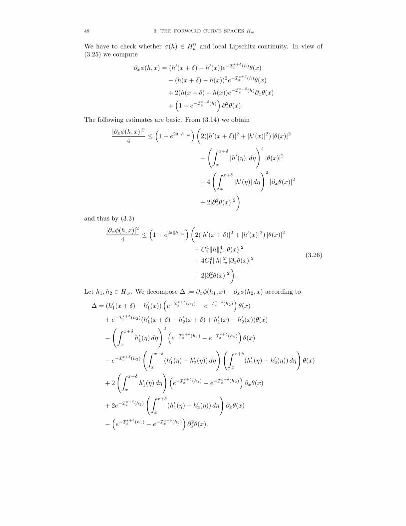
48 3. THE FORWARD CURVE SPACES Hw
We have to check whether σ(h) ∈ H0w and local Lipschitz continuity. In view of
(3.25) we compute
∂xφ(h, x) = (h′(x + δ)− h′(x))e−Ix+δx (h)θ(x)
− (h(x+ δ)− h(x))2e−Ix+δx (h)θ(x)
+ 2(h(x+ δ)− h(x))e−Ix+δx (h)∂xθ(x)
+(
1− e−Ix+δx (h)
)∂2xθ(x).
The following estimates are basic. From (3.14) we obtain
|∂xφ(h, x)|24
≤(
1 + e2δ‖h‖w)(
2(|h′(x+ δ)|2 + |h′(x)|2) |θ(x)|2
+
(∫ x+δ
x
|h′(η)| dη)4
|θ(x)|2
+ 4
(∫ x+δ
x
|h′(η)| dη)2
|∂xθ(x)|2
+ 2|∂2xθ(x)|2
)and thus by (3.3)
|∂xφ(h, x)|24
≤(
1 + e2δ‖h‖w)(
2(|h′(x+ δ)|2 + |h′(x)|2) |θ(x)|2
+ C41‖h‖4w |θ(x)|2
+ 4C21‖h‖2w |∂xθ(x)|2
+ 2|∂2xθ(x)|2
).
(3.26)
Let h1, h2 ∈ Hw. We decompose ∆ := ∂xφ(h1, x)− ∂xφ(h2, x) according to
∆ = (h′1(x+ δ)− h′1(x))(e−I
x+δx (h1) − e−I
x+δx (h2)
)θ(x)
+ e−Ix+δx (h2)(h′1(x+ δ)− h′2(x+ δ) + h′1(x) − h′2(x))θ(x)
−(∫ x+δ
x
h′1(η) dη
)2 (e−I
x+δx (h1) − e−Ix+δ
x (h2))θ(x)
− e−Ix+δx (h2)
(∫ x+δ
x
(h′1(η) + h′2(η)) dη
)(∫ x+δ
x
(h′1(η)− h′2(η)) dη
)θ(x)
+ 2
(∫ x+δ
x
h′1(η) dη
)(e−I
x+δx (h1) − e−Ix+δ
x (h2))∂xθ(x)
+ 2e−Ix+δx (h2)
(∫ x+δ
x
(h′1(η)− h′2(η)) dη
)∂xθ(x)
−(e−I
x+δx (h1) − e−I
x+δx (h2)
)∂2xθ(x).

3.6. THE BGM MODEL 49
Using ∣∣∣e−Ix+δx (h1) − e−I
x+δx (h2)
∣∣∣ ≤ δ‖h1 − h2‖weδ(‖h1‖w+‖h2‖w),
(3.3) and (3.14) we get
|∆|27≤ e2δ(‖h1‖w+‖h2‖w)
(2(|h′1(x + δ)|2 + |h′1(x)|2)δ2‖h1 − h2‖2w |θ(x)|2
+ 2(|h′1(x+ δ)− h′2(x+ δ)|2 + |h′1(x) − h′2(x)|2)|θ(x)|2
+ C41‖h1‖4wδ2‖h1 − h2‖2w |θ(x)|2
+ 2C41 (‖h1‖2w + ‖h2‖2w)‖h1 − h2‖2w |θ(x)|2
+ 4C21‖h1‖2wδ2‖h1 − h2‖2w |∂xθ(x)|2
+ 4C21‖h1 − h2‖2w |∂xθ(x)|2
+ δ2‖h1 − h2‖2w |∂2xθ(x)|2
).
(3.27)
In the sequel, C denotes a real constant which only depends on w, δ and K∗
but represents different values from line to line.In view of (3.25)∫
R+
|σ(h)′(x)|2 w(x)dx =∫ K∗δ
0
|σ(h)′(x)|2 w(x)dx
+|σ(h)(K∗δ)|2
δ2
∫ (K∗+1)δ
K∗δ
w(x)dx.
But Holder’s inequality yields
|σ(h)(K∗δ)|2 ≤(∫ K∗δ
0
|σ(h)′(x)| dx)2
≤ C(∫ K∗δ
0
|σ(h)′(x)|2 w(x)dx
),
and so, by (3.14) and (3.25)∫R+
|σ(h)′(x)|2 w(x)dx ≤ C∫ K∗δ
0
|σ(h)′(x)|2 w(x)dx
= C
K∗−1∑k=1
∫ (k+1)δ
kδ
|k∑i=1
∂xφ(h, x− iδ)|2 w(x)dx
≤ CK∗−1∑k=1
k∑i=1
∫ (k+1)δ
kδ
|∂xφ(h, x− iδ)|2 w(x)dx
≤ Cw(K∗δ)∫I
|∂xφ(h, x)|2 dx.
(3.28)
where I := [0, (K∗ − 1)δ]. In the same manner we can see that∫R+
|σ(h1)′(x) − σ(h2)′(x)|2 w(x)dx ≤ Cw(K∗δ)∫I
|∂xφ(h1, x)− ∂xφ(h2, x)|2 dx.
(3.29)

50 3. THE FORWARD CURVE SPACES Hw
From (3.26) and (3.28) it follows now easily
‖σ(h)‖2w ≤ C(
1 + e2δ‖h‖w)(‖θ‖2L∞(I) + ‖θ‖2L2(I) + ‖∂xθ‖2L2(I) + ‖∂2
xθ‖2L2(I)
)≤ C
(1 + e2δ‖h‖w
)‖∂2xθ‖2L2(I)
(3.30)
and we have used (3.24). Combining (3.27) and (3.29) gives similarly
‖σ(h1)− σ(h2)‖2w ≤ Ce2δ(‖h1‖w+‖h2‖w)‖h1 − h2‖2w ‖∂2xθ‖2L2(I). (3.31)
We are thus led to the following result.
Theorem 3.19. Let (θj(t, x))j∈N satisfyi) (t, x) 7→ θj(t, x) : R+ × I → R is jointly measurableii) θj(t, ·) ∈ C2(I), ∀t ∈ R+
iii) θj(t, 0) = ∂xθj(t, 0) = 0, ∀t ∈ R+
iv) supt∈R+
∑j∈N ‖∂2
xθj(t, ·)‖2L2(I) <∞.
Then the above construction yields a measurable mapping
σ = (σj)j∈N : (R+ ×Hw,B(R+)⊗ B(Hw))→ (L02(H0
w),B(L02(H0
w)))
which meets (3.22) and the assumptions of Lemma 3.9.i).
Proof. The structure and arguments of the proof are similar to those of theproof of Proposition 3.14. We shall give a sketch.
Condition iii) is (3.24). Estimate (3.30) and iv) clearly yield σ(t, h) ∈ L02(H0
w)and (3.15). Let g ∈ Hw. Measurability of (t, h) 7→ 〈σj(t, h), g〉w follows, using i)and ii), by similar arguments as in Step 3 in the proof of Proposition 3.14.
Finally, iv) and (3.31) imply local Lipschitz continuity of σ(t, h) in h.
The so found local HJM model is a slight modification of the BGM [12] model.The difference is that (2.22) holds for T ≤ T ∗ − δ with πj(t, T ) = θj(t, T − t).Consequently, only caplets with settlement date T+δ ≤ T ∗ can be priced accordingto formula (2.23). From a practical point of view this is no restriction at all, sinceT ∗ can be chosen arbitrarily large. From the mathematical point of view thisrestriction is essential: T ∗ = K∗δ has to be finite in estimates (3.28) and (3.29).
Unfortunately, we cannot prove existence of an HJM model which has prop-erty (3.22). In contrast to the preceding result, BGM [12] can assert global exis-tence for equation (2.25) if considered as an SPDE, see [12, Corollary 2.1]. Yet theirSPDE methods give no information about ‖rt‖w. Moreover, they do not provide ageneral framework for (local) HJM models as in the present thesis.
In summary, we have shown that the BGM [12] model is (essentially) recap-tured by our setting. In particular, it is available for the consistency results inChapter 4.
CHAPTER 4
Consistent HJM Models
4.1. Consistency Problems
In practice, the forward curve x 7→ rt(x) is often estimated by a parametrizedfamily G = G(·, z) | z ∈ Z of functions in Hw with parameter set Z ⊂ Rm,m ∈ N. By slight abuse of notation, we use the same letter G for the mappingz 7→ G(·, z) : Z → Hw. The parameter z ∈ Z is daily chosen in such a way that theforward curve x 7→ G(x, z) optimally fits the data available on the bond and swapmarket. This means that one observes the time t evolution (rt)t∈R+ of the forwardcurve by its Z-valued trace process (Zt)t∈R+ given by
G(Zt) = rt. (4.1)
Relation (4.1) implies rt ∈ G. If we assume that r is given by an HJM model(σ, γ, I) in Hw then this requires a certain consistency between (σ, γ, I) and thefamily G. This problem was first formulated by Bjork and Christensen [7]. Twoquestions naturally arise:
i) What are the conditions on (σ, γ, I) such that for any (t0, h0) ∈ R+× (I ∩G)there exists a non-trivial Z-valued process Z and (4.1) is (locally) satisfiedfor r = r(t0,h0)?
ii) If so, what kind of process is Z?Both questions are related to invertibility of (4.1) and have been studied in thesubsequent articles for exponential-polynomial families (Chapters 5–6) and for theregular but general case where G is a submanifold in Hw (Chapter 7). Accordingly,we considered different concepts of consistency.
Definition 7.8 straightly extends to the set M = G.
Definition 4.1. A local HJM model (σ, γ, I) in Hw is consistent with G ifi) G ⊂ Iii) G is locally invariant for the HJMM equation (2.25) equipped with σ.
This definition replies to question i).
Remark 4.2. It is evident that consistency is a property of σ and I only. Thisfact is also reflected by the invariance of the Nagumo type consistency conditions(7.2)–(7.3) with respect to the Girsanov transformation (2.27).
Here is a stronger version of the previous definition, which corresponds to ques-tion ii).
Definition 4.3. A local HJM model (σ, γ, I) in Hw is r-consistent1 with G ifi) G ⊂ I1This terminology is in accordance with Definition 4.1 in [7].
51

52 4. CONSISTENT HJM MODELS
ii) For any (t0, h0) ∈ R+ × G there exists a Z-valued Ito process2
Zt = Z(t0,h0)t = Z0 +
∫ t
0
bs ds+∫ t
0
ρs dW(t0)s
such that G(Z) is a local mild solution to the time t0-shifted HJMM equa-tion (2.25) equipped with σ and initial condition G(Z0) = h0.
Any such state space process Z in turn is called consistent with G if G(Z) is aglobal mild solution.3
By uniqueness of r = r(t0,h0), r-consistency of (σ, γ, I) with G implies (4.1) forr and Z = Z(t0,h0) and therefore implies consistency. The converse is not true ingeneral. In Chapter 7 we give criterions for the latter to hold. A restatement ofCorollary 3.7 and Lemma 3.9 yields their applicability. Conditions (A1)–(A5) areformulated at the end of Section 7.2.
Lemma 4.4. Suppose that σ satisfies the assumptions of Lemma 3.9.i). Then(A4) is satisfied. If in addition σ(t, ω, h) is right continuous in t ∈ R+ for allh ∈ Hw and ω ∈ Ω, then (A5) holds too.
We can now rephrase Theorem 7.13 as follows.
Theorem 4.5. Let σ satisfy (A2) and the hypotheses of Lemma 4.4. Supposethat G is an m-dimensional C2 submanifold of Hw. Then r-consistency of (σ, γ, I)with G is equivalent to consistency.
If G is linear, then the same conclusion can be drawn without assumption (A2).
There is a subtle but important difference between G being a regular or merelyan immersed submanifold.
Assume that G is a C2 immersion at some z0 ∈ Z. From Proposition A.1 wededuce that there exists an open neighborhood V of z0 in Z such that G(V ) is anm-dimensional C2 submanifold in Hw and G : V → G(V ) is a parametrization.But G can have self-intersections or can accumulate on G(V ) as shown in Figure 1.
)G(V)
(
Figure 1
Thus, in principle, G(V ) may very well fail to be consistent with (σ, γ, I) butstill (σ, γ, I) is consistent with G. The same reasoning applies for seeing that con-sistency does not imply r-consistency: even if G is an immersed submanifold, thetrace process Z may have a jump at z0 if G(z0) is an accumulation point of G.
2for some Rm-, resp. L02(Rm)-valued (F(t0)
t )-predictable processes b and ρ = (ρj)j∈N with∫ t
0
(‖bs‖Rm + ‖ρs‖2L0
2(Rm)
)ds <∞, Q-a.s. ∀t ∈ R+
3Compare with Definition 5.1, resp. Definition 6.1.

4.2. A SIMPLE CRITERION FOR REGULARITY OF G 53
On the other hand it is true that r-consistency with G implies r-consistency withG(V ). If furthermore σ satisfies the hypotheses of Theorem 4.5, then Theorem 7.13applies. We shall express the consistency conditions (7.2)–(7.3) in local coordinates,see (4.4) below. But first we have to check differentiability of G.
4.2. A Simple Criterion for Regularity of G
Consider G ∈ C2(R+ ×Z) with G(z) ≡ 4G(·, z) ∈ Hw for all z ∈ Z. We can give asimple criterion for differentiability of G in Hw.
Let ξ1, . . . , ξm denote the standard basis in Rm and let z0 ∈ Z. The partialderivative DiG(z0) is the derivative of the mapping s 7→ G(z0 + sξi) : R → Hw ins = 0. For the differential calculus in Banach spaces we refer to [1, Chapter 2]. By(H1) we have
Jx(d
dsG(z0 + sξi)|s=0
)=
d
dsJx (G(z0 + sξi)) |s=0 = ∂ziG(x, z0), x ∈ R+.
Therefore DiG(z0) = ∂ziG(·, z0) if it exists.
Lemma 4.6. Let w : R+ → [1,∞) be a non-decreasing function such thatww−1 ∈ L1 and let V be an open subset of Z. Suppose
sup(x,z)∈R+×V
|∂zi∂xG(x, z)|2w(x) <∞.
Then the partial derivatives DiG(z) exists for all z ∈ V and z 7→ DiG(z) is con-tinuous from V into Hw, for all 1 ≤ i ≤ m. Consequently, G ∈ C1(V ;Hw) and
DG(z) = (∂z1G(·, z), . . . , ∂zmG(·, z)) ∈ L(Rm;Hw). (4.2)
Proof. Let z ∈ V . Write εi = εξi, where ε > 0. We have to show that
T (ε) :=∥∥∥G(z + εi)−G(z)
ε− ∂ziG(·, z)
∥∥∥2
w→ 0 for ε→ 0.
We decompose T (ε) = T1(ε) + T2(ε), where
T1(ε) :=∣∣∣G(0, z + εi)−G(0, z)
ε− ∂ziG(0, z)
∣∣∣2 → 0 for ε→ 0
and
T2(ε) :=∫R+
∣∣∣∂xG(x, z + εi)− ∂xG(x, z)ε
− ∂zi∂xG(x, z)∣∣∣2 w(x)dx
≤∫R+
∫ 1
0
∣∣∣∂zi∂xG(x, z + sεi)− ∂zi∂xG(x, z)∣∣∣2w(x) ds dx.
For ε small enough we have z + sεi ∈ V for all s ∈ [0, 1] and by assumption∣∣∣∂zi∂xG(x, z + sεi)− ∂zi∂xG(x, z)∣∣∣2w(x) ≤ 2Cw(x)w−1(x) ∈ L1([0, 1]× R+)
where C is independent of x and ε. Hence T2(ε) → 0 for ε → 0, by dominatedconvergence. We conclude that DiG(z) exists. Continuity of z 7→ DiG(z) : V →Hw follows similarly. This proves the first part of the lemma.
For the second part we refer to [1, Proposition 2.4.12].
4Terminology introduced at the beginning of Section 4.1.

54 4. CONSISTENT HJM MODELS
By [1, Proposition 2.4.12], G ∈ C2(Z;Hw) if and only if DiG ∈ C1(Z;Hw) for1 ≤ i ≤ m, which again can be checked with Lemma 4.6. Moreover
D2G(z) =(∂zi∂zjG(·, z)
)1≤i,j≤m (4.3)
which is a bilinear mapping from Rm × Rm into Hw.
Assume that G ∈ C2(Z;Hw) and that ∂z1G(·, z0), . . . , ∂zmG(·, z0) are linearlyindependent functions, for some z0 ∈ Z. Then G is a C2 immersion at z0 and wecan go on with the reasoning at the end of the preceding section. Thus let σ meetthe hypotheses of Theorem 4.5 and let (σ, γ, I) be r-consistent with G.
By Theorem 7.9 necessarily G(V ) ∈ D(A). Combining (4.2)–(4.3) with (7.41)–(7.42) and Theorem 7.13 yields the consistency condition in local coordinates
∂xG(x, z) =m∑i=1
bi(t, ω, z)∂ziG(x, z) +12
m∑k,l=1
ak,l(t, ω, z)∂zk∂zlG(x, z)
−m∑
k,l=1
ak,l(t, ω, z)∂zkG(x, z)∫ x
0
∂zlG(η, z) dη
(4.4)
for all (t, ω, z) ∈ R+ × Ω × V (after removing a nullset from Ω). Here ak,l :=∑j∈N ρ
j,kρj,l denotes the diffusion matrix and b the drift vector of the coordinateprocess.
Compare condition (4.4) with Propositions 5.2 and 6.2. It is just the stronger(since pointwise) version of (5.4) and (6.3), respectively, which is due to the differentmeanings of “consistency” in Chapters 5–6 and Chapter 7, see Definition 4.3.
If G = G(Z) is a regular submanifold, then condition (4.4) can be used tocheck whether any local HJM model is consistent with G. In some cases this leadsto the complete characterization of all consistent local HJM models. So for regularexponential-polynomial families.
4.3. Regular Exponential-Polynomial Families
We restate the analysis of Chapters 5–6 from the preceding point of view. Asmentioned at the end of the previous section, this needs a slight modification.
Throughout this section we choose as weighting function w(x) = (1 + x)α forsome α > 3, see Example 3.4.
We adapt the notion of Section 6.3 and write
G(x, z) =K∑i=1
pi(x, z)e−zi,ni+1x (4.5)
where pi(x, z) =∑nij=0 zi,jx
j , for some vector n = (n1, . . . , nK) ∈ NK0 and K ∈ N.Since Hw contains only bounded functions, we restrict to the bounded exponential-polynomial families BEP (K,n), see Definition 6.3. But BEP (K,n) is not a sub-manifold in Hw. We have to extract the singularities. An easy computation yields
∂zi,jG(x, z) =
xje−zi,ni+1x, 0 ≤ j ≤ ni−xpi(x, z)e−zi,ni+1x, j = ni + 1.

4.3. REGULAR EXPONENTIAL-POLYNOMIAL FAMILIES 55
Hence ∂zi,jG(·, z) | 0 ≤ j ≤ ni + 1, 1 ≤ i ≤ K are linearly independent functionsif and only if
zi,ni+1 6= zj,nj+1 and zi,ni 6= 0, ∀1 ≤ i 6= j ≤ K. (4.6)
Under these constraints G(·, z) ∈ Hw if and only if zi,ni+1 > 0 or both zi,ni+1 = 0and ni = 0, compare with (6.8). But the parameter set Z has to be open. Toinclude the latter case, we will therefore assume that
n1 = 0 (4.7)z1,1 ≡ 0 and zi,ni+1 > 0 for 2 ≤ i ≤ K.
Consequently G(∞, z) = z1,0. For regularity reasons, see Remark 4.9 below, wehave to sharpen condition (4.6) and let the distance between different exponents bebounded away from zero by some fixed ε > 0. This leads to the following parameterset
Zε := R×
(z2,0, . . . , zK,nK+1)
∣∣∣∣∣∣zi,ni 6= 0,zi,ni+1 > 0,|zi,ni+1 − zj,nj+1| > ε,
∀2 ≤ i 6= j ≤ K
in Rm where m = 1 + (n2 + 2) + · · ·+ (nK + 2). To avoid self-intersections of G wefurther require that
ni 6= nj , 2 ≤ i 6= j ≤ K. (4.8)
Now the representation (4.5) of G(·, z) with z ∈ Zε is unique: G(·, z) = G(·, z) withz, z ∈ Zε implies z = z.
Definition 4.7. For K ∈ N, n ∈ NK0 satisfying (4.7)–(4.8), ε > 0 and Zε asabove we define
REP (K,n, ε) := G(Zε)the regular exponential-polynomial family.
Clearly, we have REP (K,n, ε) ⊂ BEP (K,n).Setting w(x) = (1 + x)α+2, we conclude by Lemma 4.6 that G ∈ C2(Zε, Hw).
Up to now, G : Zε → Hw is an injective immersion andREP (K,n, ε) is an immersedsubmanifold in Hw.
Proposition 4.8. The mapping G : Zε → Hw is an embedding. Its imageREP (K,n, ε) is consequently an m-dimensional C2 submanifold in Hw, with mgiven above.
Proof. We have to show that G : Zε → REP (K,n, ε) is a homeomorphism.Let (zk) be a sequence in Zε and z ∈ Zε such that G(zk) → G(z) in Hw.
Inequality (3.4) yields G(zk) → G(z) in L∞(R+). The proof is completed byshowing that zk → z.
In view of (3.3) we conclude zk1,0 = G(∞, zk) → G(∞, z) = z1,0. Thus(G(∞, zk) − zk1,0) → (G(∞, z) − z1,0) in Hw and we may assume in the sequelthat zk1,0 ≡ z1,0 = 0.
Write θi := lim supk→∞ zki,ni+1 ≤ ∞, i = 2, . . . ,K. Then there exists a subse-
quence (zkµ) of (zk) such that limµ→∞ zkµi,ni+1 = θi for all i.
Suppose first θi <∞ for all i. By definition of Zε it follows that
|θi − θj | ≥ ε, ∀2 ≤ i 6= j ≤ K. (4.9)

56 4. CONSISTENT HJM MODELS
We write N := m−K and define the RN -vectors
vµ(x) :=(e−z
kµ2,n2+1x, xe−z
kµ2,n2+1x, . . . , xn2e−z
kµ2,n2+1x, . . . , xnKe
−zkµK,nK+1x)
v(x) :=(e−θ2x, xe−θ2x, . . . , xn2e−θ2x, . . . , xnK e−θKx
)yµ :=
(zkµ2,0, z
kµ2,1, . . . , z
kµ2,n2
, . . . , zkµK,nK
).
Then
〈vµ(x), yµ〉RN = G(x, zkµ)→ G(x, z), ∀x ∈ R+. (4.10)
Fix a sequence x1 < · · · < xN in R+. The vectors vµ(x1), . . . , vµ(xN ) are linearlyindependent for any µ and so are v(x1), . . . , v(xN ), by (4.9). Hence the N × N -matrices
Mµ = Mµ(x1, . . . , xN ) :=
vµ(x1)...
vµ(xN )
, M = M(x1, . . . , xN ) :=
v(x1)...
v(xN )
are regular and Mµ →M for µ→∞. Consequently, (Mµ)−1 →M−1 and
yµ →M−1
G(x1, z)...
G(xN , z)
.
Hence yi,j := limµ→∞ zkµi,j exists in R for 0 ≤ j ≤ ni, 2 ≤ i ≤ K. We conclude
limµ→∞
G(x, zkµ) =K∑i=2
( ni∑j=1
yi,jxj)e−θix = G(x, z), ∀x ∈ R+. (4.11)
Combining (4.8) with (4.11) we get θi = zi,ni+1 and yi,j = zi,j . That way oneconcludes that any subsequence of (zk) contains a convergent subsequence withlimit z. Hence limk→∞ zk = z, and the proposition is proved in case θi <∞ for alli = 2, . . . ,K.
Now assume that I := 2 ≤ i ≤ K | θi = ∞ is not empty. Let i ∈ I. Thenthere exists x∗i ∈ R+ such that
|pi(x, zkµ)|e−zkµi,ni+1x ≤
ni∑j=0
|zkµi,j |xj(e−z
kµi,ni+1
)x→ 0 for µ→∞, ∀x ≥ x∗i .
We write N := N −∑
i∈I(ni + 1) and define the RN -vectors vµ(x), v(x) and yµ byskipping all components of vµ(x), v(x), resp. yµ which include zkµi,j or θi for i ∈ I.Set x∗ := maxi∈I x∗i . Instead of (4.10) we now have
〈vµ(x), yµ〉RN = G(x, zkµ)−∑i∈I
pi(x, zkµ)e−zkµi,ni+1x → G(x, z) ∀x ≥ x∗.
Choose a sequence x∗ ≤ x1 < · · · < xN . Inequality (4.9) still holds for i, j /∈I. Accordingly, the vectors v(x1), . . . , v(xN ) are linearly independent and so arevµ(x1), . . . , vµ(xN ) for all µ. A passage to the limit similar to the above implies
limµ→∞
G(x, zkµ) =∑i/∈I
( ni∑j=1
yi,jxj)e−θix = G(x, z), ∀x ≥ x∗,

4.3. REGULAR EXPONENTIAL-POLYNOMIAL FAMILIES 57
which is impossible since [x∗,∞) is a set of uniqueness for analytic functions. HenceI is empty, and the proof is complete.
Remark 4.9. Estimate (4.9) is essential for the preceding proof. AlthoughProposition 4.8 seems to be true also for ε = 0, we do not see how to prove itfor that case.
We can now summarize the main results from Chapter 6 as follows.
Theorem 4.10. Let σ satisfy the assumptions5 of Lemma 4.4, and suppose thelocal HJM model (σ, γ, I) is consistent with REP (K,n, ε). Then
σ(t, ω, ·) ≡ 0 on REP (K,n, ε).
Proof. The proof is divided into two steps.Step 1: Write
B :=β = (0, β2, . . . , βK) ∈ RK | βi > 0, |βi − βj | > ε, ∀2 ≤ i 6= j ≤ K
.
For β ∈ B we define
Eβ := REP (K,n, ε) ∩ spanxje−βix | 0 ≤ j ≤ ni, 1 ≤ i ≤ K
.
We claim that (σ, γ, I) is consistent with Eβ . Indeed, let (t0, h0) ∈ R+×Eβ .That is, h0 = G(z∗) with z∗ ∈ Zε and z∗i,ni+1 = βi for 1 ≤ i ≤ K. ByTheorem 7.6 there exists a Zε-valued Ito process6
Zi,jt = z∗i,j +∫ t
0
bi,js ds+∑k∈N
∫ t
0
ρi,j;ks dβks
and a stopping time τ > 0 such that r(t0,h0)t∧τ = G(Zt∧τ ) for all t ∈ R+.
Accordingly, r(t0,h0) is a local strong solution to the time t0-shifted HJMMequation (2.25). This in turn implies relation (6.3) for G(x, Z·∧τ ). By The-orem 6.4 we conclude that there exists a stopping time 0 < τ ′ ≤ τ suchthat
bi,ni+1 =∑k∈N
(ρi,ni+1;k
)2= 0, dt⊗ dQ-a.s. on [0, τ ′].
Therefore Zi,ni+1t∧τ ′ ≡ βi and the claim follows.
Step 2: Write
B := β ∈ B | 2βi = βj for some i 6= j .
The set B is contained in a finite union of hyperplanes in RK . Therefore(B \ B) ∩ B = B.
Since Eβ is a linear submanifold, Theorem 4.5 yields that (σ, γ, I) is r-consistent with Eβ . From Theorem 7.13 we derive the consistency conditionin local coordinates (4.4) which in turn implies (6.3). Hence Theorem 6.15applies and σ(t, ω, h) ≡ 0 for h ∈ Eβ , for all β ∈ B \ B. By continuity ofh 7→ σ(t, ω, h) the assertion follows.
5We don’t need (A2) here.6In fact, Z = (G−1 φ)(Y ) where φ is as in the proof of Theorem 7.6 and Y is given by
(7.27).

58 4. CONSISTENT HJM MODELS
Theorem 4.10 contains a stricter statement than Theorems 6.14–6.15. It is be-cause “consistency” in Chapter 6 is only related to one particular initial point h0
in REP (K,n, ε), see Definition 6.1 and Proposition 6.2 and compare with Defini-tions 4.1–4.3.
Let’s recall the two leading examples of Chapters 5–6.
4.3.1. The Nelson–Siegel Family.
GNS(x, z) = z1,0 + (z2,0 + z2,1x)e−z2,2x
In the preceding context we have GNS(Zε) = REP (2, (0, 1), ε), where actually ε isredundant.
4.3.2. The Regular Svensson Family.
GS(x, z) = z1,0 + (z2,0 + z2,1x)e−z2,2x + z3,1xe−z3,2x
Obviously, condition (4.8) is not satisfied. So the preceding discussion does notapply immediately. Yet we can “regularize” also the Svensson family. Set ε > 0and
ZS,ε := R× (z2,0, z2,1, z2,2, z3,1, z3,2) | |z2,0| > ε, z2,2, z3,2 > 0, |z2,2 − z3,2| > ε.
Similar as in the proof of Proposition 4.8 one shows that GS : ZS,ε → Hw isan embedding. As before we conclude σ(t, ω, h) ≡ 0 for h ∈ GS(ZS,ε), for everyconsistent local HJM model (σ, γ, I).
In Section 6.9.2 we identify the coordinate process Z for the non-trivial HJMmodel7 which is r-consistent with the full (bounded) Svensson family. It is amazingthat the support of the non-deterministic component Z2,0
t contains 0 for arbitrarysmall t (it is Gaussian distributed). Thus P[Zt /∈ ZS,ε] > 0 for every t > 0. However,as far as I can see, there is no deeper connection between failure of (4.8) and theexistence of a non-trivial consistent state space process for the Svensson family.
Remark 4.11. Consistency of HJM models with exponential-polynomial fami-lies has been checked first by Bjork and Christensen [7] for deterministic σ. Theirresult was extended by the two articles in Chapter 5 and 6. There, however, wemerely checked r-consistency for EP (K,n), resp. BEP (K,n). Question ii) in Sec-tion 4.1, asserting the generality of that approach, was left open and it is nowclarified by Theorem 4.10.
4.4. Affine Term Structure
In this section we apply Theorem 7.13 to identify the particular class of affine localHJM models . That is, those local HJM models which are consistent with finitedimensional linear submanifolds.
It is required throughout that σ meets the assumptions of Lemma 4.4. Supposethat M is an m-dimensional linear submanifold of Hw which is locally invariantfor the HJMM equation (2.25). Without loss of generality, M is connected. Ac-cording to Theorem 7.10 there exists V ⊂ Rm open and connected and a globalparametrization φ : V →M with φ(y) = g0 +
∑mi=1 yigi where g0, . . . , gm ∈ D(A)
are linearly independent. Clearly Dφ(y) ≡ (g1, . . . , gm).
7It’s a generalized Vasicek model.

4.4. AFFINE TERM STRUCTURE 59
Applying Theorem 7.13 yields, see (4.4),
g′0 +m∑i=1
yig′i =
m∑i=1
bi(t, ω, y)gi −12
m∑i,j=1
ai,j(t, ω, y)GiGj
′ (4.12)
for all (t, ω, y) ∈ R+ × Ω× V (after removing a P-nullset from Ω), where Gi(x) :=∫ x0 gi(η) dη. To shorten notation, we let ′ stand for ∂x.
Write γi = gi(0). Integrating (4.12) yields
g0 − γ0 +m∑i=1
yi(gi − γi) =m∑i=1
bi(t, ω, y)Gi −12
m∑i,j=1
ai,j(t, ω, y)GiGj . (4.13)
Now if Gi and GiGj , 1 ≤ i, j ≤ m, are linearly independent functions, we caninvert the linear equation (4.13) for bi(t, ω, y) and ai,j(t, ω, y). Since the left handside of (4.13) is affine in y, we obtain that also they are affine functions in y:
bi(t, ω, y) = bi(t, ω) +m∑j=1
βi,j(t, ω)yj, 1 ≤ i ≤ m
ai,j(t, ω, y) = ai,j(t, ω) +m∑k=1
αi,j,k(t, ω)yk, 1 ≤ i, j ≤ m
for some predictable functions bi(t, ω), βi,j(t, ω), ai,j(t, ω) and αi,j,k(t, ω) beingright continuous in t.
Since affine functions are analytic and V is open, equation (4.13) splits into thefollowing system of Riccati equations for the Gi’s
G′0 = γ0 +m∑k=1
bk(t, ω)Gk −12
m∑k,l=1
ak,l(t, ω)GkGl
G′i = γi +m∑k=1
βk,i(t, ω)Gk −12
m∑k,l=1
αk,l,i(t, ω)GkGl, 1 ≤ i ≤ m(4.14)
with initial conditions G0(0) = · · · = Gm(0) = 0.Hence we derived some of the results in [21] as a special case of our general
point of view. Clearly, Theorem 7.13 imposes constraints on the choice of V in orderthat b and ρ are locally Lipschitz, see (7.44), and that (7.43) has a local solution inV . Moreover, there is a tradeoff between the functions gi and the coefficients ai,j ,αi,j,k, bi, βi,j and γi by the Riccati equations (4.14). We shall discuss this problemfor the case m = 1. For a fuller treatment we refer to [21].
For simplicity we assume that there is only a one dimensional driving Brownianmotion W and that all coefficients are autonomous, that is
b(t, ω, y) ≡ b1(y) = b+ βy
a(t, ω, y) ≡ a1,1(y) = a+ αy.
Accordingly
ρ(t, ω, y) ≡ ρ1,1(y) =√a+ αy.

60 4. CONSISTENT HJM MODELS
We rewrite the Riccati equations (4.14) for G0 and G1:
G′0 = γ0 + bG1 −12aG2
1, G0(0) = 0
G′1 = γ1 + βG1 −12αG2
1, G1(0) = 0. (4.15)
Equation (4.15) admits a non-exploding solutionG1 : R+ → R if and only if αγ1 ≥ 0or both αγ1 < 0 and β ≤ −
√2|αγ1|.
Suppose α > 0. Theorem 7.13 tells us that y 7→ √a+ αy has to be locallyLipschitz in V , see (7.44). Consequently, a+αy has to be bounded away from zero.Thus V ⊂ [ ε−aα ,∞) for some ε > 0. The dynamics of the coordinate process, see(7.43), is given by the stochastic differential equation
dYt = (b+ βYt) dt+√a+ αYt dWt, Y0 ∈ V. (4.16)
It can be shown8, see [29, p. 221], that (4.16) admits a (global) unique continuousstrong solution on [−aα ,∞) if b ≥ a
αβ.If α < 0, then V ⊂ (−∞, ε−aα ] for some ε > 0 and (4.16) remains valid.
4.4.1. The Cox–Ingersoll–Ross (CIR) Model. For α > 0, γ1 = 1 anda = γ0 = 0 (and hence b ≥ 0) we get the CIR [17] short rate model. There existsa closed form solution to (4.15), see [17, Formula (23)],
G1(x) =2(e
(√β2+2α
)x − 1
)(√
β2 + 2α− β)(
e
(√β2+2α
)x − 1
)+ 2√β2 + 2α
and G0(x) = b∫ x
0 G1(η) dη. It holds by inspection9 that g0 = G′0 = bG1 ∈ Hw andg1 = G′1 ∈ H0
w for any polynomial weighting function w as in Example 3.4. Hencethe CIR model is contained in our setting.
From (7.41) and the identity y = g0(0) + yg1(0) = J0(φ(y)) we obtain
σ(t, ω, h) ≡ σ1(h) =√αJ0(h) g1, h ∈ φ((0,∞)).
Denote by σ : Hw → H0w a measurable continuation of σ. Let Y be the continuous
solution of (4.16) with Y0 > ε and write τε = inft | Yt ≤ ε. It is straightforwardthat (rt∧τε) = (φ(Yt∧τε)) with r0 = φ(Y0) is the unique continuous local strongsolution to the HJMM equation (2.25) equipped with σ, see Theorem 7.13
However, σ(h) – and hence σ(h) – cannot be extended Lipschitz continuously toh = φ(0) (naturally σ(φ(0)) = 0). Thus, although φ(Y ) is a strong solution to theHJMM equation (2.25) with σ(φ(0)) = 0, we cannot assert its global uniqueness.Uniqueness, however, holds for Y in R+, by the preceding discussion.
8Substitute X := Y + aα
9More general it can be shown that the critical point y0 =β+√β2+2αα
∈ R+ for (4.15)
is globally exponentially stable, see [2, Chapter IV]. A fact which also applies for the multi-dimensional system (4.14). We will investigate this further in connection with general affinemodels.

4.4. AFFINE TERM STRUCTURE 61
4.4.2. The Vasicek Model. The case α = 0 leads to a Gaussian coordinateprocess Y . There are no constraints on V , but a has to be non-negative.
For γ0 = 0, γ1 = 1, b ≥ 0 and β < 0 this is the Vasicek [48] short rate model.The solution for (4.15) is given by
G1(x) =1β
(eβx − 1
)and G0(x) = b
∫ x0G1(η) dη − 1
2a∫ x
0G2
1(η) dη. Obviously, g0 = bG1 − 12aG
21 ∈ Hw
and g1(x) = eβx ∈ H0w. Hence also this classical model is contained in our setting.
From (7.41) we deduce that σ(t, ω, h) ≡ σ1(h) ≡√ag1 for h ∈ φ(R).


Part 2
Publications


CHAPTER 5
A Note on the Nelson–Siegel Family
ABSTRACT. We study a problem posed in Bjork and Christensen [7]: doesthere exist any nontrivial interest rate model which is consistent with theNelson–Siegel family? They show that within the HJM framework withdeterministic volatility structure the answer is no.
In this paper we give a generalized version of this result including sto-chastic volatility structure. For that purpose we introduce the class of consis-tent state space processes, which have the property to provide an arbitrage-free interest rate model when representing the parameters of the Nelson–Siegel family. We characterize the consistent state space Ito processes interms of their drift and diffusion coefficients. By solving an inverse prob-lem we find their explicit form. It turns out that there exists no nontrivialinterest rate model driven by a consistent state space Ito process.
5.1. Introduction
Bjork and Christensen [7] introduce the following concept: letM be an interest ratemodel and G a parameterized family of forward curves. M and G are called consis-tent, if all forward rate curves which may be produced by M are contained withinG, provided that the initial forward rate curve lies in G. Under the assumption ofa deterministic volatility structure and working under a martingale measure, theyshow that within the Heath–Jarrow–Morton (henceforth HJM) framework thereexists no nontrivial forward rate model, consistent with the Nelson–Siegel familyG( . , z). The curve shape of G( . , z) is given by the well known expression
G(x, z) = z1 + z2e−z4x + z3xe
−z4x, (5.1)
introduced by Nelson and Siegel [39].For an optimal todays choice of the parameter z ∈ R4, expression (5.1) rep-
resents the current term structure of interest rates, i.e. x ≥ 0 denotes time tomaturity. This method of fitting the forward curve is widely used among centralbanks, see the BIS [6] documentation.
From an economic point of view it seems reasonable to restrict z to the statespace Z := z = (z1, . . . , z4) ∈ R4 | z4 > 0.
The corresponding term structure of the bond prices is given by
Π(x, z) := exp(−∫ x
0
G(η, z) dη).
Then Π ∈ C∞([0,∞)×Z).In order to imply a stochastic evolution of the forward rates, we introduce in
Section 5.2 some state space process Z = (Zt)0≤t<∞ with values in Z and askwhether G( . , Z) provides an arbitrage-free interest rate model. We call Z consis-tent, if the corresponding discounted bond prices are martingales, see Section 5.3.
65

66 5. A NOTE ON THE NELSON–SIEGEL FAMILY
Solving an inverse problem we characterize in Section 5.4 the class of consistentstate space Ito processes. Since a diffusion is a special Ito process, the very im-portant class of consistent state space diffusion processes is characterized as well.Still we are able to derive a more general result. It turns out that all consistent Itoprocesses have essentially deterministic dynamics. The corresponding interest ratemodels are in turn trivial.
Consistent state space Ito processes are, by definition, specified under a mar-tingale measure. This seems to be a restriction at first and one may ask whetherthere exists any Ito process Z under some objective probability measure inducinga nontrivial arbitrage free interest rate model G( . , Z). However if the underlyingfiltration is not too large we show in Section 5.5 that our (negative) result holdsfor Ito processes modeled under any probability measure, provided that there ex-ists an equivalent martingale measure. Hence under the requirement of absence ofarbitrage there exists no nontrivial interest rate model driven by Ito processes andconsistent with the Nelson–Siegel family.
Using the same ideas, still larger classes of consistent processes like Ito processeswith jumps could be characterized.
5.2. The Interest Rate Model
For the stochastic background and notations we refer to [40] and [31].Let (Ω,F , (Ft)0≤t<∞,P) be a filtered complete probability space, satisfying
the usual conditions, and let W = (W 1t , . . . ,W
dt )0≤t<∞ denote a standard d-
dimensional (Ft)-Brownian motion, d ≥ 1.We assume as given a Z-valued Ito process Z = (Z1, . . . , Z4) of the form
Zit = Zi0 +∫ t
0
bis ds+d∑j=1
∫ t
0
σijs dWjs , i = 1, . . . , 4, 0 ≤ t <∞, (5.2)
where Z0 is F0-measurable, and b, σ are progressively measurable processes withvalues in R4, resp. R4×d, such that∫ t
0
(|bs|+ |σs|2
)ds <∞, P-a.s., for all finite t. (5.3)
Z could be for instance the (weak) solution of a stochastic differential equation,but in general Z is not Markov.
Write r(t, x) := G(x, Zt) for the instantaneous forward rate prevailing at timet for date t+ x.
It is shown in [19, Section 7] that traded assets have to follow semimartingales.Hence it is of importance for us to observe that the price at time t for a zero couponbond with maturity T
P (t, T ) := Π(T − t, Zt), 0 ≤ t ≤ T <∞,and the short rates
r(t, 0) = limx→0
r(t, x) = G(0, Zt) = − ∂
∂xΠ(0, Zt), 0 ≤ t <∞,
form continuous semimartingales, by the smoothness of G and Π. Therefore thesame holds for the process of the savings account
B(t) := exp(∫ t
0
r(s, 0) ds), 0 ≤ t <∞.
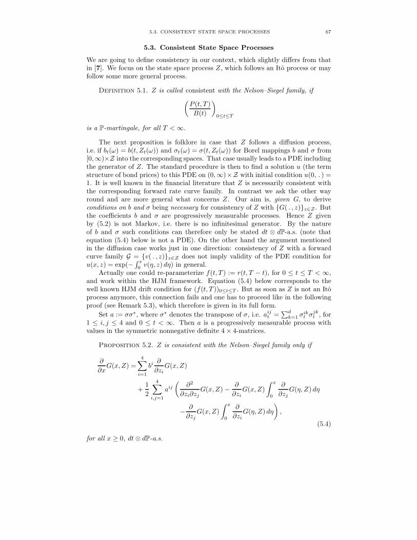
5.3. CONSISTENT STATE SPACE PROCESSES 67
5.3. Consistent State Space Processes
We are going to define consistency in our context, which slightly differs from thatin [7]. We focus on the state space process Z, which follows an Ito process or mayfollow some more general process.
Definition 5.1. Z is called consistent with the Nelson–Siegel family, if(P (t, T )B(t)
)0≤t≤T
is a P-martingale, for all T <∞.
The next proposition is folklore in case that Z follows a diffusion process,i.e. if bt(ω) = b(t, Zt(ω)) and σt(ω) = σ(t, Zt(ω)) for Borel mappings b and σ from[0,∞)×Z into the corresponding spaces. That case usually leads to a PDE includingthe generator of Z. The standard procedure is then to find a solution u (the termstructure of bond prices) to this PDE on (0,∞)×Z with initial condition u(0, . ) =1. It is well known in the financial literature that Z is necessarily consistent withthe corresponding forward rate curve family. In contrast we ask the other wayround and are more general what concerns Z. Our aim is, given G, to deriveconditions on b and σ being necessary for consistency of Z with G( . , z)z∈Z . Butthe coefficients b and σ are progressively measurable processes. Hence Z givenby (5.2) is not Markov, i.e. there is no infinitesimal generator. By the natureof b and σ such conditions can therefore only be stated dt ⊗ dP-a.s. (note thatequation (5.4) below is not a PDE). On the other hand the argument mentionedin the diffusion case works just in one direction: consistency of Z with a forwardcurve family G = v( . , z)z∈Z does not imply validity of the PDE condition foru(x, z) = exp(−
∫ x0v(η, z) dη) in general.
Actually one could re-parameterize f(t, T ) := r(t, T − t), for 0 ≤ t ≤ T < ∞,and work within the HJM framework. Equation (5.4) below corresponds to thewell known HJM drift condition for (f(t, T ))0≤t≤T . But as soon as Z is not an Itoprocess anymore, this connection fails and one has to proceed like in the followingproof (see Remark 5.3), which therefore is given in its full form.
Set a := σσ∗, where σ∗ denotes the transpose of σ, i.e. aijt =∑dk=1 σ
ikt σ
jkt , for
1 ≤ i, j ≤ 4 and 0 ≤ t < ∞. Then a is a progressively measurable process withvalues in the symmetric nonnegative definite 4× 4-matrices.
Proposition 5.2. Z is consistent with the Nelson–Siegel family only if
∂
∂xG(x, Z) =
4∑i=1
bi∂
∂ziG(x, Z)
+12
4∑i,j=1
aij(
∂2
∂zi∂zjG(x, Z)− ∂
∂ziG(x, Z)
∫ x
0
∂
∂zjG(η, Z) dη
− ∂
∂zjG(x, Z)
∫ x
0
∂
∂ziG(η, Z) dη
),
(5.4)
for all x ≥ 0, dt⊗ dP-a.s.

68 5. A NOTE ON THE NELSON–SIEGEL FAMILY
Proof. For f ∈ C2(Z) we set
At(ω)f(z) :=4∑i=1
bit(ω)∂f
∂zi(z) +
12
4∑i,j=1
aijt (ω)∂2f
∂zi∂zj(z), 0 ≤ t <∞, z ∈ Z.
Using Ito’s formula we get for T <∞
P (t, T ) = P (0, T ) +∫ t
0
(AsΠ(T − s, Zs)−
∂
∂xΠ(T − s, Zs)
)ds
+∫ t
0
σ∗s∇zΠ(T − s, Zs) dWs, 0 ≤ t ≤ T, P-a.s.
where ∇z denotes the gradient with respect to (z1, z2, z3, z4), and
1B(t)
= 1 +∫ t
0
1B(s)
∂
∂xΠ(0, Zs) ds, 0 ≤ t <∞, P-a.s.
For 0 ≤ t ≤ T define
H(t, T ) :=1
B(t)
(AtΠ(T − t, Zt)−
∂
∂xΠ(T − t, Zt) +
∂
∂xΠ(0, Zt)Π(T − t, Zt)
)and the local martingale
M(t, T ) :=∫ t
0
1B(s)
σ∗s∇zΠ(T − s, Zs) dWs.
Integration by parts then yields
1B(t)
P (t, T ) = P (0, T ) +∫ t
0
H(s, T ) ds+M(t, T ), 0 ≤ t ≤ T, P-a.s.
Let’s suppose now that Z is consistent. Then necessarily for T <∞∫ t
0
H(s, T ) ds = 0, ∀t ∈ [0, T ], P-a.s. (5.5)
Since b and σ are progressive and Π is smooth, H( . , T ) is progressively measurableon [0, T ]× Ω. We claim that (5.5) yields
H( . , T ) = 0, on [0, T ]× Ω, dt⊗ dP-a.s. (5.6)
Proof of (5.6). Define N := (t, ω) ∈ [0, T ] × Ω | H(t, T )(ω) > 0. Then N is aB⊗F- measurable set. Since H( . , T ) is positive on N we can use Tonelli’s theorem∫
N
H(t, T )(ω) dt⊗ dP =∫
Ω
(∫Nω
H(t, T )(ω) dt)dP(ω) = 0,
where Nω := t | (t, ω) ∈ N ∈ B and we have used (5.5) and the inner regularityof the measure dt. We therefore conclude that N has dt ⊗ dP-measure zero. Byusing a similar argument for −H( . , T ) we have proved (5.6).
Note that (5.6) holds for all T < ∞, where the dt ⊗ dP-nullset depends on T .But since H(t, T ) is continuous in T , a standard argument yields
H(t, t+ x)(ω) = 0, ∀x ≥ 0, for dt⊗ dP-a.e. (t, ω).
Multiplying this equation with B(t) and using again the full form this reads
AΠ(x, Z) − ∂
∂xΠ(x, Z) +
∂
∂xΠ(0, Z)Π(x, Z) = 0, ∀x ≥ 0, dt⊗ dP-a.s. (5.7)
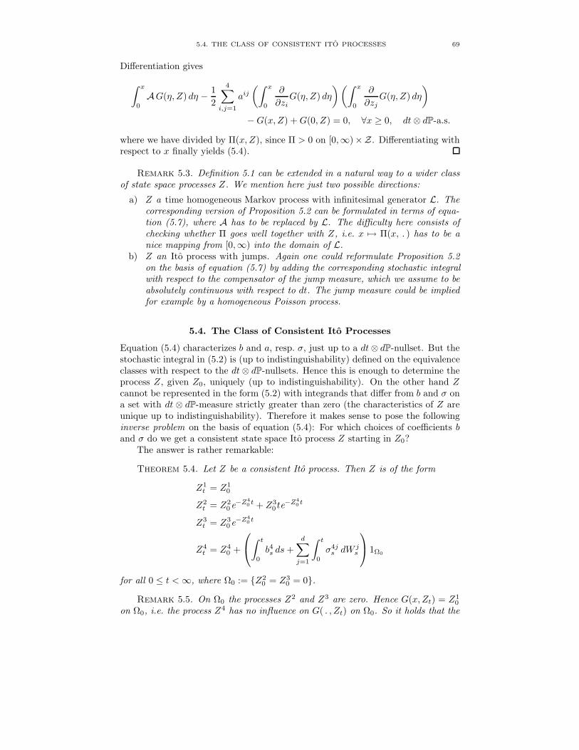
5.4. THE CLASS OF CONSISTENT ITO PROCESSES 69
Differentiation gives∫ x
0
AG(η, Z) dη − 12
4∑i,j=1
aij(∫ x
0
∂
∂ziG(η, Z) dη
)(∫ x
0
∂
∂zjG(η, Z) dη
)−G(x, Z) +G(0, Z) = 0, ∀x ≥ 0, dt⊗ dP-a.s.
where we have divided by Π(x, Z), since Π > 0 on [0,∞)×Z. Differentiating withrespect to x finally yields (5.4).
Remark 5.3. Definition 5.1 can be extended in a natural way to a wider classof state space processes Z. We mention here just two possible directions:
a) Z a time homogeneous Markov process with infinitesimal generator L. Thecorresponding version of Proposition 5.2 can be formulated in terms of equa-tion (5.7), where A has to be replaced by L. The difficulty here consists ofchecking whether Π goes well together with Z, i.e. x 7→ Π(x, . ) has to be anice mapping from [0,∞) into the domain of L.
b) Z an Ito process with jumps. Again one could reformulate Proposition 5.2on the basis of equation (5.7) by adding the corresponding stochastic integralwith respect to the compensator of the jump measure, which we assume to beabsolutely continuous with respect to dt. The jump measure could be impliedfor example by a homogeneous Poisson process.
5.4. The Class of Consistent Ito Processes
Equation (5.4) characterizes b and a, resp. σ, just up to a dt⊗ dP-nullset. But thestochastic integral in (5.2) is (up to indistinguishability) defined on the equivalenceclasses with respect to the dt⊗ dP-nullsets. Hence this is enough to determine theprocess Z, given Z0, uniquely (up to indistinguishability). On the other hand Zcannot be represented in the form (5.2) with integrands that differ from b and σ ona set with dt ⊗ dP-measure strictly greater than zero (the characteristics of Z areunique up to indistinguishability). Therefore it makes sense to pose the followinginverse problem on the basis of equation (5.4): For which choices of coefficients band σ do we get a consistent state space Ito process Z starting in Z0?
The answer is rather remarkable:
Theorem 5.4. Let Z be a consistent Ito process. Then Z is of the form
Z1t = Z1
0
Z2t = Z2
0e−Z40 t + Z3
0 te−Z4
0 t
Z3t = Z3
0e−Z40 t
Z4t = Z4
0 +
∫ t
0
b4s ds+d∑j=1
∫ t
0
σ4js dW j
s
1Ω0
for all 0 ≤ t <∞, where Ω0 := Z20 = Z3
0 = 0.
Remark 5.5. On Ω0 the processes Z2 and Z3 are zero. Hence G(x, Zt) = Z10
on Ω0, i.e. the process Z4 has no influence on G( . , Zt) on Ω0. So it holds that the

70 5. A NOTE ON THE NELSON–SIEGEL FAMILY
corresponding interest rate model is of the form
r(t, x) = G(x, Zt)
= Z10 +
(Z2
0e−Z4
0 t + Z30 te−Z4
0 t)e−Z
40x + Z3
0e−Z4
0 txe−Z40x
= Z10 + Z2
0e−Z4
0 (t+x) + Z30 (t+ x)e−Z
40(t+x)
= r(0, t+ x), ∀t, x ≥ 0,
and is therefore quasi deterministic, i.e. all randomness remains F0-measurable.
Remark 5.6. One can show a similar (negative) result even for the wider classof state space Ito processes with jumps on a finite or countable mark space, seeRemark 5.3. However allowing for more general exponential-polynomial familiesG( . , z) there exist (although very restricted) consistent Ito processes providing anontrivial interest rate model, see [23].
Proof. Let Z be a consistent Ito process given by equation (5.2). The proofof the theorem relies on expanding equation (5.4).
First of all we subtract ∂∂xG(x, Z) from both sides of (5.4) to obtain a null
equation. Fix then a point (t, ω) in [0,∞)×Ω. For simplicity we write (z1, z2, z3, z4)for Zt(ω), aij for aijt (ω) and bi for bit(ω). Notice that Zt(ω) ∈ Z, i.e. z4 > 0. Observethen that our null equation is in fact of the form
p1(x) + p2(x)e−z4x + p3(x)e−2z4x = 0, (5.8)
which has to hold simultaneously for all x ≥ 0. The expressions p1, p2 and p3 denotesome polynomials in x, which depend on the zi’s, bi’s and aij ’s. Since the functions1, e−z4x, e−2z4x are independent over the ring of polynomials, (5.8) can only besatisfied if each of the pi’s is 0. This again yields that all coefficients of the pi’shave to be zero. To proceed in our analysis we list all terms appearing in (5.4):
∂
∂xG(x, z) = (−z2z4 + z3 − z3z4x)e−z4x,
∇zG(x, z) =(1, e−z4x, xe−z4x, (−z2x− z3x
2)e−z4x),
∂2
∂zi∂zjG(x, z) = 0, for 1 ≤ i, j ≤ 3,
∂
∂z4∇zG(x, z) =
(0,−xe−z4x,−x2e−z4x, (z2x
2 + z3x3)e−z4x
).
Finally we need the relation∫ x
0
ηme−z4η dη = −qm(x)e−z4x +m!zm+1
4
, m = 0, 1, 2, . . . ,
where qm(x) =∑mk=0
m!(m−k)!
xm−k
zk+14
is a polynomial in x of order m.First we shall analyze p1. The terms that contribute to p1 are those containing
∂∂z1
G(x, z) and ∂∂z1
G(x, z)∫ x
0∂∂zj
G(η, z) dη, for 1 ≤ j ≤ 4. Actually p1 is of theform
p1(x) = a11x+ · · ·+ b1,
where . . . stands for terms of zero order in x containing the factors a1j = aj1, for1 ≤ j ≤ 4. It follows that a11 = 0. But the matrix (aij) has to be nonnegative

5.4. THE CLASS OF CONSISTENT ITO PROCESSES 71
definite, so necessarily
a1j = aj1 = 0, for all 1 ≤ j ≤ 4,
and therefore also b1 = 0. Thus p1 is done.The contributing terms to p3 are those containing ∂
∂ziG(x, z)
∫ x0
∂∂zj
G(η, z) dη,for 2 ≤ i, j ≤ 4. But observe that the degree of p3 and p2 depends on whether z2
or z3 are equal to zero or not. Hence we have to distinguish between the four cases
i) z2 6= 0, z3 6= 0 iii) z2 = 0, z3 6= 0
ii) z2 6= 0, z3 = 0 iv) z2 = z3 = 0.
case i): The degree of p3 is 4. The fourth order coefficient contains a44, i.e.
p3(x) = a44z 2
3
z4x4 + . . . ,
where . . . stands for terms of lower order in x. Hence
a4j = aj4 = 0, for 1 ≤ j ≤ 4.
The degree of p3 reduces to 2. The second order coefficient is a33z4
. Hencea3j = aj3 = 0, for 1 ≤ j ≤ 4. It remains p3(x) = a22
z4. Thus the diffusion
matrix (aij) is zero. This implies that (σij) is zero, independent of the choiceof d (the number of Brownian motions in (5.2)). Now we can write down p2:
p2(x) = −b4z3x2 + (b3 − b4z2 + z3z4)x+ b2 + z2z4 − z3.
It follows that b4 = 0 and
b2 = z3 − z2z4,
b3 = −z3z4.
For the other three cases we will need the following lemma, which is a directconsequence of the occupation times formula, see [40, Corollary (1.6), Chapter VI].
Lemma 5.7. Using the same notation as in (5.2), it holds for 1 ≤ i ≤ 4 that
aii1Zi=0 = bi1Zi=0 = 0, dt⊗ dP-a.s.
As a consequence, since we are characterizing a and b up to a dt⊗ dP-nullset,we may and will assume that zi = 0 implies aij = aji = bi = 0, for 1 ≤ j ≤ 4 andi = 2, 3.
case ii): We have ∇zG(x, z) = (1, e−z4x, xe−z4x,−z2xe−z4x). Hence the degree
of p3 is 2. Since a3j = aj3 = b3 = 0, for 1 ≤ j ≤ 4, the second order coefficientcomes from
−a44∂
∂z4G(x, z)
∫ x
0
∂
∂z4G(η, z) dη = a44
z 22
z4x2e−2z4x + . . . ,
where . . . denotes terms of lower order in x. Hence a4j = aj4 = 0, for1 ≤ j ≤ 4. The polynomial p3 reduces to p3(x) = a22
z4. It follows that also in
this case the diffusion matrix (aij) is zero. From case i) we derive immediatelythat now
p2(x) = −b4z2x+ b2 + z2z4,
hence b2 = −z2z4 and b4 = 0.
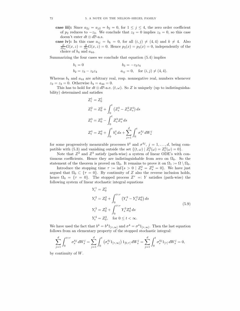
72 5. A NOTE ON THE NELSON–SIEGEL FAMILY
case iii): Since a2j = aj2 = b2 = 0, for 1 ≤ j ≤ 4, the zero order coefficientof p2 reduces to −z3. We conclude that z2 = 0 implies z3 = 0, so this casedoesn’t enter dt⊗ dP-a.s.
case iv): In this case aij = bk = 0, for all (i, j) 6= (4, 4) and k 6= 4. Also∂∂z4
G(x, z) = ∂∂xG(x, z) = 0. Hence p2(x) = p3(x) = 0, independently of the
choice of b4 and a44.
Summarizing the four cases we conclude that equation (5.4) implies
b1 = 0 b3 = −z3z4
b2 = z3 − z2z4 aij = 0, for (i, j) 6= (4, 4).
Whereas b4 and a44 are arbitrary real, resp. nonnegative real, numbers wheneverz2 = z3 = 0. Otherwise b4 = a44 = 0.
This has to hold for dt⊗ dP-a.e. (t, ω). So Z is uniquely (up to indistinguisha-bility) determined and satisfies
Z1t = Z1
0
Z2t = Z2
0 +∫ t
0
(Z3s − Z2
sZ4s
)ds
Z3t = Z3
0 −∫ t
0
Z3sZ
4s ds
Z4t = Z4
0 +∫ t
0
b4s ds+d∑j=1
∫ t
0
σ4js dW j
s
for some progressively measurable processes b4 and σ4j , j = 1, . . . , d, being com-patible with (5.3) and vanishing outside the set (t, ω) | Z2
t (ω) = Z3t (ω) = 0.
Note that Z2 and Z3 satisfy (path-wise) a system of linear ODE’s with con-tinuous coefficients. Hence they are indistinguishable from zero on Ω0. So thestatement of the theorem is proved on Ω0. It remains to prove it on Ω1 := Ω \ Ω0.
Introduce the stopping time τ := infs > 0 | Z2s = Z3
s = 0. We have justargued that Ω0 ⊂ τ = 0. By continuity of Z also the reverse inclusion holds,hence Ω0 = τ = 0. The stopped process Zτ =: Y satisfies (path-wise) thefollowing system of linear stochastic integral equations
Y 1t = Z1
0
Y 2t = Z2
0 +∫ t∧τ
0
(Y 3s − Y 2
s Z40
)ds
Y 3t = Z3
0 +∫ t∧τ
0
Y 3s Z
40 ds
Y 4t = Z4
0 , for 0 ≤ t <∞.
(5.9)
We have used the fact that b4 = b41[τ,∞] and σ4 = σ41[τ,∞]. Then the last equationfollows from an elementary property of the stopped stochastic integral:
d∑j=1
∫ t∧τ
0
σ4js dW j
s =d∑j=1
∫ t
0
(σ4js 1[τ,∞]
)1[0,τ ] dW
js =
d∑j=1
∫ t
0
σ4js 1[τ ] dW
js = 0,
by continuity of W .

5.5. E-CONSISTENT ITO PROCESSES 73
The system (5.9) has the unique solution for 0 ≤ t <∞Y 1t = Z1
0
Y 2t = Z2
0e−Z4
0(t∧τ) + Z30 (t ∧ τ)e−Z
40 (t∧τ)
Y 3t = Z3
0e−Z4
0(t∧τ)
Y 4t = Z4
0 .
Since Z = Y on the stochastic interval [0, τ ] and since Yt 6= 0, ∀t < ∞, P-a.s. onΩ1, it follows by the continuity of Z, that Ω1 = τ > 0 = τ =∞. Inserting thisin the above solution, the theorem is proved also on Ω1.
5.5. E-Consistent Ito Processes
Note that by definition Z is consistent if and only if P is a martingale measure forthe discounted bond price processes. We could generalize this definition and call astate space process Z e-consistent if there exists an equivalent martingale measureQ. Then obviously consistency implies e-consistency, and e-consistency implies theabsence of arbitrage opportunities, as it is well known.
In case where the filtration is generated by the Brownian motion W , i.e. (Ft) =(FWt ), we can give the following stronger result:
Proposition 5.8. If (Ft) = (FWt ), then any e-consistent Ito process Z is ofthe form as stated in Theorem 5.4. In particular the corresponding interest ratemodel is purely deterministic.
Proof. Let Z be an e-consistent Ito process under P, and let Q be an equiv-alent martingale measure. Since (Ft) = (FWt ), we know that all P-martingaleshave the representation property relative to W . By Girsanov’s theorem it followstherefore that Z remains an Ito process under Q. In particular Z is a consistentstate space Ito process with respect to the stochastic basis (Ω,F , (FWt )0≤t<∞,Q).Hence Z is of the form as stated in Theorem 5.4.
Since FW0 consists of sets of measure 0 or 1, the processes Z1, Z2, Z3 are (afterchanging the Zi0’s on a set of measure 0) purely deterministic and therefore also(r(t, . ))0≤t<∞, see Remark 5.5.


CHAPTER 6
Exponential-Polynomial Families and the Term
Structure of Interest Rates
ABSTRACT. Exponential-polynomial families like the Nelson–Siegel or Svens-son family are widely used to estimate the current forward rate curve. Weinvestigate whether these methods go well with inter-temporal modelling.We characterize the consistent Ito processes which have the property to pro-vide an arbitrage free interest rate model when representing the parametersof some bounded exponential-polynomial type function. This includes inparticular diffusion processes. We show that there is a strong limitation ontheir choice. Bounded exponential-polynomial families should rather not beused for modelling the term structure of interest rates.
6.1. Introduction
The current term structure of interest rates contains all the necessary informationfor pricing bonds, swaps and forward rate agreements of all maturities. It is usedfurthermore by the central banks as indicator for their monetary policy.
There are several algorithms for constructing the current forward rate curvefrom the (finitely many) prices of bonds and swaps observed in the market. Widelyused are splines and parameterized families of smooth curves G( . , z)z∈Z , whereZ ⊂ RN , N ≥ 1, denotes some finite dimensional parameter set. By an optimalchoice of the parameter z in Z an optimal fit of the forward curve x 7→ G(x, z) tothe observed data is attained. Here x ≥ 0 denotes time to maturity. In that sensez represents the current state of the economy taking values in the state space Z.
Examples are the Nelson–Siegel [39] family with curve shape
GNS(x, z) = z1 + (z2 + z3x)e−z4x
and the Svensson [44] family, an extension of Nelson–Siegel,
GS(x, z) = z1 + (z2 + z3x)e−z5x + z4xe−z6x.
Table 1 gives an overview of the fitting procedures used by some selected centralbanks. It is taken from the documentation of the Bank for International Settle-ments [6].
Despite the flexibility and low number of parameters of GNS and GS , theirchoice is somewhat arbitrary. We shall discuss them from an inter-temporal point ofview: A lot of cross-sectional data, i.e. daily estimations of z, is available. Thereforeit would be natural to ask for the stochastic evolution of the parameter z over time.But then there exist economic constraints based on no arbitrage considerations.
75

76 6. EXPONENTIAL-POLYNOMIAL FAMILIES
Table 1. Forward rate curve fitting procedures
central bank curve fitting procedureBelgium Nelson–Siegel, SvenssonCanada SvenssonFinland Nelson–SiegelFrance Nelson–Siegel, SvenssonGermany SvenssonItaly Nelson–SiegelJapan smoothing splinesNorway SvenssonSpain Nelson–Siegel (before 1995), SvenssonSweden SvenssonUK SvenssonUSA smoothing splines
Following [7], instead of GNS and GS we consider general exponential-poly-nomial families containing curves of the form
G(x, z) =K∑i=1
( ni∑µ=0
zi,µxµ)e−zi,ni+1x.
Hence linear combinations of exponential functions exp(−zi,ni+1x) over some poly-nomials of degree ni ∈ N0. Obviously GNS and GS are of this type. We replacethen z by an Ito process Z = (Zt)t≥0 taking values in Z. The following questionsarise:• Does G( . , Z) provide an arbitrage free interest rate model?• And what are the conditions on Z for it?Working in the Heath–Jarrow–Morton [28] – henceforth HJM – framework
with deterministic volatility structure, Bjork and Christensen [7] showed that theexponential-polynomial families are in a certain sense to large to carry an interestrate model. This result has been generalized for the Nelson–Siegel family in [25],including stochastic volatility structure. Expanding the methods used in there, wegive in this paper the general result for bounded exponential-polynomial families.
The paper is organized as follows. In Section 6.2 we introduce the class of Itoprocesses consistent with a given parameterized family of forward rate curves. Con-sistent Ito processes provide an arbitrage free interest rate model when driving theparameterized family. They are characterized in terms of their drift and diffusioncoefficients by the HJM drift condition.
By solving an inverse problem we get the main result for consistent Ito pro-cesses, stated in Section 6.3. It is shown that they are remarkably limited. Theproof is divided into several steps, given in Sections 6.4, 6.5 and 6.6.
In Section 6.7 we extend the notion of consistency to e-consistency when P isnot a martingale measure.
The main result reads much clearer when restricting to diffusion processes, asshown in Section 6.8. It turns out that e-consistent diffusion processes drivingbounded exponential-polynomial families like Nelson–Siegel or Svensson are verylimited: Most of the factors are either constant or deterministic. It is shown in

6.2. CONSISTENT ITO PROCESSES 77
Section 6.9, that there is no non-trivial diffusion process which is e-consistent withthe Nelson–Siegel family. Furthermore we identify the diffusion process which ise-consistent with the Svensson family. It contains just one non deterministic com-ponent. The corresponding short rate model is shown to be the generalized Vasicekmodel.
We conclude that bounded exponential-polynomial families, in particular GNSand GS , should rather not be used for modelling the term structure of interestrates.
6.2. Consistent Ito Processes
For the stochastic background and notations we refer the reader to [40] and [31].Let (Ω,F , (Ft)0≤t<∞,P) be a filtered complete probability space, satisfying theusual conditions, and letW = (W 1
t , . . . ,Wdt )0≤t<∞ denote a standard d-dimensional
(Ft)-Brownian motion, d ≥ 1.Let Z = (Z1, . . . , ZN) denote an RN–valued Ito process, N ≥ 1, of the form
Zit = Zi0 +∫ t
0
bis ds+d∑j=1
∫ t
0
σi,js dW js , i = 1, . . . , N, 0 ≤ t <∞,
where Z0 is F0-measurable, and b, σ are progressively measurable processes withvalues in RN , resp. RN×d, such that∫ t
0
(|bs|+ |σs|2
)ds <∞, P-a.s., for all finite t.
Let G(x, z) be a function in C1,2(R+ × RN ), i.e. G and the partial derivatives(∂G/∂x), (∂G/∂zi), (∂2G/∂zi∂zj), which exist for 1 ≤ i, j ≤ N , are continuousfunctions on R+×RN . Interpreting Zt as the state of the economy at time t, we letx 7→ G(x, Zt) stand for the corresponding term structure of interest rates. Meaningthat G(x, Zt) denotes the instantaneous forward rate at time t for date t+ x.
Notice that
Π(x, z) := exp(−∫ x
0
G(η, z) dη)
is in C1,2(R+ × RN ) too. Therefore the price processes for zero coupon T -bonds
P (t, T ) := Π(T − t, Zt), 0 ≤ t ≤ T <∞, (6.1)
and the process of the savings account
B(t) := exp(−∫ t
0
∂
∂xΠ(0, Zs) ds
), 0 ≤ t <∞,
form continuous semimartingales.Let Z denote an arbitrary subset of RN . The function G generates in a canon-
ical way a parameterized set of forward curves G( . , z)z∈Z . We shall refer to Zas the state space of the economy.
Definition 6.1. Z is called consistent with G( . , z)z∈Z , if the support of Zis contained in Z and (
P (t, T )B(t)
)0≤t≤T
(6.2)
is a P-martingale, for all T <∞.

78 6. EXPONENTIAL-POLYNOMIAL FAMILIES
Set a := σσ∗, where σ∗ denotes the transpose of σ, i.e. ai,jt =∑d
k=1 σi,kt σj,kt ,
for 1 ≤ i, j ≤ N and 0 ≤ t <∞. Then a is a progressively measurable process withvalues in the symmetric nonnegative definite N ×N -matrices.
Using Ito’s formula, the dynamics of (6.2) can be decomposed into finite vari-ation and local martingale part. Requiring consistency the former has to vanish.This is the well known HJM drift condition and is stated explicitly in the followingproposition.
Proposition 6.2. If Z is consistent with G( . , z)z∈Z then
∂
∂xG(x, Z) =
N∑i=1
bi∂
∂ziG(x, Z)
+12
N∑i,j=1
ai,j(
∂2
∂zi∂zjG(x, Z)− ∂
∂ziG(x, Z)
∫ x
0
∂
∂zjG(η, Z) dη
− ∂
∂zjG(x, Z)
∫ x
0
∂
∂ziG(η, Z) dη
),
(6.3)
for all x ≥ 0, dt⊗ dP-a.s.
Proof. Analogous to the proof of Proposition 5.2.
6.3. Exponential-Polynomial Families
In this section we introduce a particular class of functions G. As the main resultwe characterize the corresponding consistent Ito processes.
Let K denote a positive integer and let n = (n1, . . . , nK) be a vector withcomponents ni ∈ N0, for 1 ≤ i ≤ K. Write |n| := n1 + · · ·+ nK . For a point
z = (z1,0, . . . , z1,n1+1, z2,0, . . . , z2,n2+1, . . . , zK,0, . . . , zK,nK+1) ∈ R|n|+2K (6.4)
define the polynomials pi(z) as
pi(z) = pi(x, z) :=ni∑µ=0
zi,µxµ, 1 ≤ i ≤ K.
The function G is now defined as
G(x, z) :=K∑i=1
pi(x, z)e−zi,ni+1x. (6.5)
Obviously G ∈ C1,2(R+ × R|n|+2K). Hence the preceding section applies withN = |n|+ 2K.
From an economic point of view it seems reasonable to restrict to boundedforward rate curves. Let therefore Z denote the set of all z ∈ RN such thatsupx∈R+
|G(x, z)| <∞.
Definition 6.3. The exponential-polynomial family EP (K,n) is defined asthe set of forward curves G( . , z)z∈RN .
The bounded exponential-polynomial family BEP (K,n) ⊂ EP (K,n) is de-fined as the set of forward curves G( . , z)z∈Z .

6.3. EXPONENTIAL-POLYNOMIAL FAMILIES 79
Clearly GNS(x, z) ∈ BEP (2, (0, 1)) and GS(x, z) ∈ BEP (3, (0, 1, 1)), if at eachcase the parameter z is chosen such that the curve is bounded. From now on, theNelson–Siegel and Svensson families are considered as subsets of BEP (2, (0, 1)) andBEP (3, (0, 1, 1)) respectively.
If two exponents zi,ni+1 and zj,nj+1 coincide, the sum (6.5) defining G reducesto a linear combination of K − 1 exponential functions. Thus for z ∈ RN weintroduce the equivalence relation
i ∼z j :⇐⇒ zi,ni+1 = zj,nj+1 (6.6)
on the set 1, . . . ,K and denote by [i] = [i]z the equivalence class of i. We willuse the notation
n[i] = n[i](z) := maxnj | j ∈ [i]zI[i],µ = I[i],µ(z) := j ∈ [i]z | nj ≥ µ, 0 ≤ µ ≤ n[i](z)
z[i],µ = z[i],µ(z) :=∑
j∈I[i],µ(z)
zj,µ, 0 ≤ µ ≤ n[i](z)
p[i](z) :=∑j∈[i]z
pj(z).
(6.7)
In particular p[i](z) =∑n[i]
µ=0 z[i],µxµ and (6.5) reads now
G(x, z) =∑
[i]∈1,...,K/∼
p[i](z)e−zi,ni+1x.
Observe that for z ∈ Z we havezi,ni+1 = 0, only if p[i](z) = z[i],0
zi,ni+1 < 0, only if p[i](z) = 0.(6.8)
We shall write the RN -valued Ito process Z with the same indices which weuse for a point z ∈ RN , see (6.4),
Zi,µt = Zi,µ0 +∫ t
0
bi,µs ds+d∑
λ=1
∫ t
0
σi,µ;λs dWλ
s , 0 ≤ µ ≤ ni + 1, 1 ≤ i ≤ K.
(6.9)
It’s diffusion matrix a consists of the components
ai,µ;j,ν =d∑
λ=1
σi,µ;λσj,ν;λ, 0 ≤ µ ≤ ni + 1, 0 ≤ ν ≤ nj + 1, 1 ≤ i, j ≤ K.
Notice that for 1 ≤ i ≤ K
z | p[i](z) = 0 =⋃
J⊂1,...,KJ3i
(z | zj,nj+1 = zi,ni+1 for all j ∈ J
∩maxnj |j∈J⋂
µ=0
z |∑j∈Jnj≥µ
zj,µ = 0
\⋃l∈Jcz | zl,nl+1 = zi,ni+1
)(6.10)

80 6. EXPONENTIAL-POLYNOMIAL FAMILIES
is not closed in general but nevertheless a Borel set in RN . We introduce thefollowing, thus optional, random sets of singular points (t, ω)
Ai :=pi(Z) = 0 or p[i](Z) = 0
, 1 ≤ i ≤ K
B :=K⋃
i,j=1i6=j
Zi,ni+1 = Zj,nj+1
C :=K⋃
i,j=1i6=j
2Zi,ni+1 = Zj,nj+1
and the optional random sets of regular points (t, ω)
D := (R+ × Ω) \ (K⋃i=1
Ai ∪ B ∪ C)
D′ := (R+ × Ω) \ (B ∪ C).Let us recall that for S and T stopping times, a stochastic interval like [S, T ] is
a subset of R+×Ω. Hence [S] = [S, S] is the restriction of the graph of the mappingS : Ω→ [0,∞] to the set R+ × Ω.
For any stopping time τ with [τ ] ∈ (R+ × Ω) \ Ai we define
τ ′(ω) := inft > τ(ω) | (t, ω) ∈ Ai,the debut of the optional set [τ,∞[∩Ai. Observe that in general it is not true thatτ ′ > τ on τ <∞. This can be seen from the following example: For
G(x, z) = z1,0e−z1,1x + z2,0e
−z2,1x + z3,0e−z3,1x ∈ BEP (3, (0, 0, 0))
let Z1,0t = Z3,0
t = 1, Z2,0t = −1, Z3,1
t = 1+t and Z1,1t = Z2,1
t = 1 for t ∈ [0, 1]. Thenp1(Z0) = p[1](Z0) = 1 and p[1](Zt) = 0 for all t ∈ (0, 1]. Hence [0] ∈ (R+ ×Ω) \ A1,but τ ′ = 0. However, by continuity of Z we always have
τ < τ ′ P-a.s. on ω | (τ(ω), ω) ∈ D′. (6.11)
Recall the fact that there is a one to one correspondence between the Ito pro-cesses Z starting in Z0 (up to indistinguishability) and the equivalence classes ofb and σ with respect to the dt ⊗ dP-nullsets in R+ ⊗ F . Hence we may state thefollowing inverse problem to equation (6.3): Given a family of forward curves. Forwhich choices of coefficients b and σ do we get a consistent Ito process Z startingin Z0?
The main result is the following characterization of all consistent Ito processes,which is remarkably restrictive. The proof of the theorem will be given in Sections6.5 and 6.6.
Theorem 6.4. Let K ∈ N, n = (n1, . . . , nK) ∈ NK0 and Z as above. If Z isconsistent with BEP (K,n), then necessarily for 1 ≤ i ≤ K
ai,ni+1;i,ni+1 = 0, on pi(Z) 6= 0, dt⊗ dP-a.s. (6.12)
bi,ni+1 = 0, on pi(Z) 6= 0 ∩ p[i](Z) 6= 0, dt⊗ dP-a.s. (6.13)
Consequently, Zi,ni+1 is constant on intervals where pi(Z) 6= 0 and p[i](Z) 6= 0.That is, for P-a.e. ω
Zi,ni+1t (ω) = Zi,ni+1
u (ω) for t ∈ [u, v],

6.4. AUXILIARY RESULTS 81
if pi(Zt(ω)) 6= 0 and p[i](Zt(ω)) 6= 0 for t ∈ (u, v).For a stopping time τ with [τ ] ⊂ D′ let τ ′(ω) := inft ≥ τ(ω) | (t, ω) /∈
D′ denote the debut of the optional random set (B ∪ C) ∩ [τ,∞[. Then it holdsfurthermore that τ < τ ′ on τ <∞ and
Zi,µτ+t = Zi,µτ e−Zi,ni+1τ t + Zi,µ+1
τ te−Zi,ni+1τ t
Zi,niτ+t = Zi,niτ e−Zi,ni+1τ t
on [0, τ ′ − τ [, for 0 ≤ µ ≤ ni − 1 and 1 ≤ i ≤ K, up to evanescence.If D′ above is replaced by D and τ ′ is the debut of (∪Ki=1Ai ∪ B ∪ C) ∩ [τ,∞[,
then τ ′ =∞ and in addition
Zi,ni+1τ+t = Zi,ni+1
τ
for 1 ≤ i ≤ K, P-a.s. on τ <∞.Remark 6.5. It will be made clear in the proof of the theorem that it is actually
sufficient to assume Z to be consistent with EP (K,n) for (6.12) to hold.
As an immediate consequence we may state the following corollaries. Thenotation is the same as in the theorem.
Corollary 6.6. If Z is consistent with BEP (K,n) and if the optional randomsets pi(Z) = 0 and p[i](Z) = 0 have dt ⊗ dP-measure zero, then the exponentZi,ni+1 is indistinguishable from Zi,ni+1
0 , 1 ≤ i ≤ K.
Proof. If pi(Z) = 0 and p[i](Z) = 0 have dt ⊗ dP-measure zero, thenpi(Z) 6= 0 ∩ p[i](Z) 6= 0 = R+ × Ω up to a dt ⊗ dP-nullset. The claim followsusing (6.12) and (6.13).
Corollary 6.7. If Z is consistent with BEP (K,n) and if the following threepoints are P-a.s. satisfied
i) pi(Z0) 6= 0, for all 1 ≤ i ≤ K,ii) there exists no pair of indices i 6= j with Zi,ni+1
0 = Zj,nj+10 ,
iii) there exists no pair of indices i 6= j with 2Zi,ni+10 = Z
j,nj+10 ,
then Z and hence the interest rate model G(x, Z) is quasi deterministic, i.e. allrandomness remains F0-measurable. In particular the exponents Zi,ni+1 are indis-tinguishable from Zi,ni+1
0 , for 1 ≤ i ≤ K.
Proof. If i), ii) and iii) hold P-a.s. then [0] ⊂ D. The claim follows from thesecond part of the theorem setting τ = 0.
6.4. Auxiliary Results
For the proof of the main result we need three auxiliary lemmas, presented inthis section. First there is a result on the identification of the coefficients of Itoprocesses.
Lemma 6.8. Let
Xt = X0 +∫ t
0
βXs ds+d∑j=1
∫ t
0
γX,js dW js
Yt = Y0 +∫ t
0
βYs ds+d∑j=1
∫ t
0
γY,js dW js

82 6. EXPONENTIAL-POLYNOMIAL FAMILIES
be two Ito processes. Then dt⊗ dP-a.s.
1X=Y
d∑j=1
(γX,j)2 = 1X=Y
d∑j=1
γX,jγY,j = 1X=Y
d∑j=1
(γY,j)2
1X=Y βX = 1X=Y β
Y .
Proof. We write 〈 . , . 〉 for the scalar product in Rd. Then
|〈γX , γX〉 − 〈γX , γY 〉| = |〈γX , γX − γY 〉| ≤√〈γX , γX〉
√〈γX − γY , γX − γY 〉
By the occupation times formula, see [40, Corollary (1.6), Chapter VI],∫ t
0
1Xs=Ys〈γXs − γYs , γXs − γYs 〉 ds = 0, for all t <∞, P-a.s.
Hence by Holder inequality∫ t
0
1Xs=Ys|〈γXs , γXs 〉 − 〈γXs , γYs 〉| ds
≤∫ t
0
1Xs=Ys√〈γXs , γXs 〉
√〈γXs − γYs , γXs − γYs 〉 ds
≤(∫ t
0
1Xs=Ys〈γXs , γXs 〉 ds) 1
2(∫ t
0
1Xs=Ys〈γXs − γYs , γXs − γYs 〉 ds) 1
2
= 0, for all t <∞, P-a.s.
Thus by symmetry
1X=Y 〈γX , γX〉 = 1X=Y 〈γX , γY 〉 = 1X=Y 〈γY , γY 〉, dt⊗ dP-a.s.
By continuity of the processes X and Y there are sequences of stopping times(Sn) and (Tn), Sn ≤ Tn, with [Sm, Tm] ∩ [Sn, Tn] = ∅ for all m 6= n and
X = Y =⋃n∈N
[Sn, Tn], up to evanescence.
To see this, let n ∈ N and let S(n, 1) := inft > 0 | |Xt − Yt| = 0. DefineT (n, p) := inft > S(n, p) | |Xt − Yt| > 0 and inductively
S(n, p+ 1) := inft > S(n, p) | |Xt − Yt| = 0 and supS(n,p)≤s≤t |Xs − Ys| > 2−n.Then by continuity we have limp→∞ S(n, p) = ∞ for all n ∈ N and it follows thatX = Y =
⋃n,p∈N[S(n, p), T (n, p)]. Now proceed as in [31, Lemma I.1.31] to find
the sequences (Sn) and (Tn) with the desired properties.From above we have 1X=Y (γX − γY )2 = 0, dt⊗ dP-a.s. For any 0 ≤ t < ∞
therefore∫ Tn∧tSn∧t (γXs − γYs ) dWs = 0, P-a.s. Hence
0 = (X − Y )Tn∧t − (X − Y )Sn∧t =∫ Tn∧t
Sn∧t(βXs − βYs ) ds, P-a.s.
We conclude∫ t
0
1Xs=Ys(βXs − βYs ) ds =
∑n∈N
∫ Tn∧t
Sn∧t(βXs − βYs ) ds = 0, for 0 ≤ t <∞, P-a.s.
Using the same arguments as in the proof of [25, Proposition 3.2], we derive thedesired result.

6.4. AUXILIARY RESULTS 83
Secondly there are listed two results in matrix algebra.
Lemma 6.9. Let γ = (γi,j) be a N × d-matrix and define the symmetric non-negative definite N × N -matrix α := γγ∗, i.e. αi,j = αj,i =
∑dλ=1 γi,λγj,λ. Let I
and J denote two arbitrary subsets of 1, . . . , N. Define
αI,J = αJ,I :=∑j∈J
∑i∈I
αi,j .
Then it holds that αI,I ≥ 0 and |αI,J | ≤√αI,I√αJ,J .
Proof. For 1 ≤ λ ≤ d define γI,λ :=∑i∈I γi,λ. Then by definition
αI,J =∑j∈J
∑i∈I
d∑λ=1
γi,λγj,λ =d∑
λ=1
(∑i∈I
γi,λ
)(∑j∈J
γj,λ
)=
d∑λ=1
γI,λγJ,λ.
Hence
αI,I =d∑
λ=1
(γI,λ)2 ≥ 0
and by Schwarz inequality
|αI,J | ≤
√√√√ d∑λ=1
(γI,λ)2
√√√√ d∑λ=1
(γJ,λ)2 =√αI,I√αJ,J .
Lemma 6.10. Let α = (αi,j) be a n × n-matrix, n ∈ N, which is diagonallydominant from the right, i.e.
|αi,i| ≥n∑j=1j 6=i
|αi,j |
|αi,i| >n∑
j=i+1
|αi,j |,(
setn∑
j=n+1
· · · := 0),
for all 1 ≤ i ≤ n. Then α is regular.
Proof. The proof is a slight modification of an argument given in [42, Theo-rem 1.5].
Gaussian elimination: by assumption |α1,1| >∑nj=2 |α1,j | ≥ 0, in particular
α1,1 6= 0. If n = 1 we are done. If n > 1, the elimination step
α(1)i,j := αi,j −
αi,1α1,1
α1,j, 2 ≤ i, j ≤ n,
leads to the (n − 1) × (n − 1)-matrix α(1) = (α(1)i,j )2≤i,j≤n. We show that α(1) is
diagonal dominant from the right. If αi,1 = 0, there is nothing to prove for the i-throw. Let αi,1 6= 0, for some 2 ≤ i ≤ n. We have
|α(1)i,j | ≥ |αi,j | −
∣∣∣∣αi,1α1,1
∣∣∣∣ |α1,j |, 2 ≤ j ≤ n.
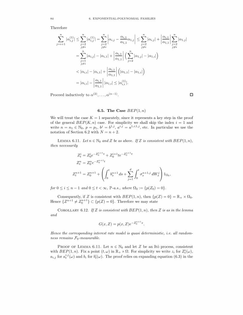
84 6. EXPONENTIAL-POLYNOMIAL FAMILIES
Therefore
n∑j=i+1
|α(1)i,j | ≤
n∑j=2j 6=i
|α(1)i,j | =
n∑j=2j 6=i
∣∣∣∣αi,j − αi,1α1,1
α1,j
∣∣∣∣ ≤ n∑j=2j 6=i
|αi,j |+∣∣∣∣αi,1α1,1
∣∣∣∣ n∑j=2j 6=i
|α1,j |
=n∑j=1j 6=i
|αi,j | − |αi,1|+∣∣∣∣αi,1α1,1
∣∣∣∣ ( n∑j=2
|α1,j | − |α1,i|)
< |αi,i| − |αi,1|+∣∣∣∣αi,1α1,1
∣∣∣∣ (|α1,1| − |α1,i|)
= |αi,i| −∣∣∣∣αi,1α1,1
∣∣∣∣ |α1,i| ≤ |α(1)i,i |.
Proceed inductively to α(2), . . . , α(n−1).
6.5. The Case BEP (1, n)
We will treat the case K = 1 separately, since it represents a key step in the proofof the general BEP (K,n) case. For simplicity we shall skip the index i = 1 andwrite n = n1 ∈ N0, p = p1, bj = b1,j, ai,j = a1,i;1,j , etc. In particular we use thenotation of Section 6.2 with N = n+ 2.
Lemma 6.11. Let n ∈ N0 and Z be as above. If Z is consistent with BEP (1, n),then necessarily
Zit = Zi0e−Zn+1
0 t + Zi+10 te−Z
n+10 t
Znt = Zn0 e−Zn+1
0 t
Zn+1t = Zn+1
0 +
∫ t
0
bn+1s ds+
d∑j=1
∫ t
0
σn+1,js dW j
s
1Ω0 ,
for 0 ≤ i ≤ n− 1 and 0 ≤ t <∞, P-a.s., where Ω0 := p(Z0) = 0.
Consequently, if Z is consistent with BEP (1, n), then p(Z) = 0 = R+ × Ω0.Hence Zn+1 6= Zn+1
0 ⊂ p(Z) = 0. Therefore we may state
Corollary 6.12. If Z is consistent with BEP (1, n), then Z is as in the lemmaand
G(x, Z) = p(x, Z)e−Zn+10 x.
Hence the corresponding interest rate model is quasi deterministic, i.e. all random-ness remains F0-measurable.
Proof of Lemma 6.11. Let n ∈ N0 and let Z be an Ito process, consistentwith BEP (1, n). Fix a point (t, ω) in R+×Ω. For simplicity we write zi for Zit(ω),ai,j for ai,jt (ω) and bi for bit(ω). The proof relies on expanding equation (6.3) in the

6.5. THE CASE BEP (1, n) 85
point z = (z0, . . . , zn+1). The involved terms are
∂
∂xG(x, z) =
(∂
∂xp(x, z)− zn+1p(x, z)
)e−zn+1x (6.14)
∂
∂ziG(x, z) =
xie−zn+1x, 0 ≤ i ≤ n−xp(x, z)e−zn+1x, i = n+ 1
(6.15)
∂2G(x, z)∂zi∂zj
=∂2G(x, z)∂zj∂zi
=
0, 0 ≤ i, j ≤ n−xi+1e−zn+1x, 0 ≤ i ≤ n, j = n+ 1x2p(x, z)e−zn+1x, i = j = n+ 1.
(6.16)
Finally it’s useful to know the following relation for m ∈ N0∫ x
0
ηme−zn+1η dη =
−qm(x)e−zn+1x + m!
zm+1n+1
, zn+1 6= 0xm+1
m+1 , zn+1 = 0,(6.17)
where qm(x) =∑mk=0
m!(m−k)!
xm−k
zk+1n+1
is a polynomial in x of order m.
Let’s suppose first that zn+1 6= 0. Thus, subtracting ∂∂xG(x, Z) from both sides
of (6.3) we get a null equation of the form
q1(x)e−zn+1x + q2(x)e−2zn+1x = 0, (6.18)
which has to hold simultaneously for all x ≥ 0. The polynomials q1 and q2 dependon the zi’s, bi’s and ai,j ’s. Equality (6.18) implies q1 = q2 = 0. This again yieldsthat all coefficients of the qi’s have to be zero.
To proceed we have to distinguish the two cases p(z) 6= 0 and p(z) = 0. Let’ssuppose first the former is true. Then there exists an index i ∈ 0, . . . , n such thatzi 6= 0. Set m := maxi ≤ n | zi 6= 0. With regard to (6.15)–(6.17) it follows thatdeg q2 = 2m+ 2. In particular
q2(x) = an+1,n+1z2m
zn+1x2m+2 + . . . ,
where . . . denotes terms of lower order in x. Hence an+1,n+1 = 0. But the matrixa has to be nonnegative definite, so necessarily
an+1,j = aj,n+1 = 0, for all 1 ≤ j ≤ n+ 1.
In view of Lemma 6.8 (setting Y = 0), since we are characterizing a and b up todt⊗dP-nullsets, we may assume ai,j = aj,i = 0, for 0 ≤ j ≤ n+ 1, for all i ≥ m+ 1.Thus the degree of q2 reduces to 2m. Explicitly
q2(x) =am,mzn+1
x2m + . . . .
Hence am,m = 0 and so am,j = aj,m = 0, for 0 ≤ j ≤ n+ 1. Proceeding inductivelyfor i = m−1,m−2, . . . , 0 we finally get that the diffusion matrix a is equal to zeroand hence q2 = 0 is fulfilled.
Now we determine the drift b. By Lemma 6.8, we may assume bi = 0 form+ 1 ≤ i ≤ n. With regard to (6.14) and (6.15), q1 reduces therefore to
q1(x) = −bn+1zmxm+1 + . . . .

86 6. EXPONENTIAL-POLYNOMIAL FAMILIES
It follows bn+1 = 0 and it remains
q1(x) = (bm + zn+1zm)xm +m−1∑i=0
(bi − zi+1 + zn+1zi)xi
= (bn + zn+1zn)xn +n−1∑i=0
(bi − zi+1 + zn+1zi)xi.
We now turn to the singular cases. If p(z) = 0, that is z0 = · · · = zn = 0, wemay assume ai,j = aj,i = bi = 0, 0 ≤ j ≤ n+ 1, for all i ≤ n. But this means thatq1 = q2 = 0, independently of the choice of bn+1 and an+1,n+1.
For the case where zn+1 = 0 we need the boundedness assumption z ∈ Z. By(6.8) it follows that z1 = · · · = zn = 0. So by Lemma 6.8 again ai,j = aj,i = bi = 0,0 ≤ j ≤ n+ 1, for all i ≥ 1. Thus in this case equation (6.3) reduces to
0 = b0 − a0,0x
and therefore b0 = a0,0 = 0.
Summarizing all cases we conclude that necessarily
bi = −zn+1zi + zi+1, 0 ≤ i ≤ n− 1bn = −zn+1zn
ai,j = 0, for (i, j) 6= (n+ 1, n+ 1).
Whereas bn+1 and an+1,n+1 are arbitrary real, resp. nonnegative real, numberswhenever p(z) = 0. Otherwise bn+1 = an+1,n+1 = 0.
The rest of the proof is analogous to the proof of [25, Proposition 4.1].
6.6. The General Case BEP (K,n)
Using again the notation of Section 6.3 we give the proof of the main result forthe case K ≥ 2. The exposure is somewhat messy, which is due to the multi-dimensionality of the problem. The idea however is simple: For a fixed point(t, ω) ∈ R+×Ω we expand equation (6.3), which turns out to be a linear combinationof linearly independent exponential functions over the ring of polynomials, equalingzero. Consequently many of the coefficients have to vanish, which leads to ourassertion.
The difficulty is that some exponents may coincide. This causes a considerablenumber of singular cases which require a separate discussion.
Proof of Theorem 6.4. Let K ≥ 2, n = (n1, . . . , nK) ∈ NK0 , and let Z beconsistent with BEP (K,n). As in the proof of Lemma 6.11 we fix a point (t, ω) inR+ × Ω and use the shorthand notation zi,µ for Zi,µt (ω), ai,µ;j,ν for ai,µ;j,ν
t (ω) andbi,µ for bi,µt (ω), etc. Since we are characterizing a and b up to a dt⊗ dP-nullset, weassume that (t, ω) is chosen outside of an exceptional dt⊗ dP-nullset. In particularthe lemmas from Section 6.4 shall apply each time we use them.
The strategy is the same as for the case K = 1. Thus we expand equation (6.3)in the point z = (z1,0, . . . , zK,nK+1) to get a linear combination of (ideally) linearly

6.6. THE GENERAL CASE BEP (K,n) 87
independent exponential functions over the ring of polynomialsK∑i=1
qi(x)e−zi,ni+1x +∑
1≤i≤j≤Kqi,j(x)e−(zi,ni+1+zj,nj+1)x = 0. (6.19)
Consequently, all polynomials qi and qi,j have to be zero. The main difference tothe case K = 1 is that representation (6.19) may not be unique due to the possiblymultiple occurrence of the following singular cases
i) zi,ni+1 = zj,nj+1, for i 6= j,ii) 2zi,ni+1 = zj,nj+1 + zk,nk+1,iii) 2zi,ni+1 = zj,nj+1,iv) zi,ni+1 = zj,nj+1 + zk,nk+1,
for some indices 1 ≤ i, j, k ≤ K. However, the lemmas in Section 6.4 and theboundedness assumption z ∈ Z are good enough to settle these four cases.
Let’s suppose first that pi(z) 6= 0, for all i ∈ 1, . . . ,K. To settle Case i),let ∼ denote the equivalence relation defined in (6.6). After re-parametrization ifnecessary we may assume that
1, . . . ,K/∼ = [1], . . . , [K]and z1,n1+1 < · · · < zK,nK+1 for some integer K ≤ K. Write I := 1, . . . , K. Inview of Lemma 6.8 we may assume
aj,nj+1;j,nj+1 = ai,ni+1;i,ni+1 and bj,nj+1 = bi,ni+1 for all j ∈ [i], i ∈ I. (6.20)
The proof of (6.12) and (6.13) is divided into four claims.
Claim 1. ai,ni+1;i,ni+1 = 0, for all i ∈ I.
Expression (6.19) takes the form∑i∈I
qi(x)e−zi,ni+1x +∑i,j∈Ii≤j
qi,j(x)e−(zi,ni+1+zj,nj+1)x = 0, (6.21)
for some polynomials qi and qi,j . Taking into account Cases ii)–iv), this repre-sentation may still not be unique. However if for an index i ∈ I there exist noj, k ∈ I such that 2zi,ni+1 = zj,nj+1 + zk,nk+1 or 2zi,ni+1 = zj,nj+1 (in particularzi,ni+1 6= 0) then we have
qi,i(x) = ai,ni+1;i,ni+1
∑j∈I[i],µm
z2j,µm
zi,ni+1x2µm+2 + . . . ,
where µm := maxν | ν ≤ nj and zj,ν 6= 0 for some j ∈ [i] ∈ N0. Henceai,ni+1;i,ni+1 = 0 and Claim 1 is proved for the regular case.
For the singular cases observe first that zi,ni+1 = 0 implies ai,ni+1;i,ni+1 = 0,which follows from Lemma 6.8. Now we split I into two disjoint subsets I1 and I2,where
I1 := i ∈ I | zi,ni+1 6= 0 and there exist j, k ∈ I, such that
2zi,ni+1 = zj,nj+1 + zk,nk+1 or 2zi,ni+1 = zj,nj+1I2 := I \ I1.
Observe that zK,nK+1 > 0 implies K ∈ I2 and z1,n1+1 < 0 implies 1 ∈ I2. Since atleast one of these events has to happen, the set I2 is not empty. We have shown

88 6. EXPONENTIAL-POLYNOMIAL FAMILIES
above that ai,ni+1;i,ni+1 = 0, for i ∈ I2. If I1 is not empty, we will show that foreach i ∈ I1, the parameter zi,ni+1 can be written as a linear combination of zj,nj+1’swith j ∈ I2. From this it follows by Lemmas 6.8 and 6.9 that ai,ni+1;i,ni+1 = 0for all i ∈ I1 and Claim 1 is completely proved. We proceed as follows. WriteI1 = i1, . . . , ir with zi1,ni1+1 < · · · < zir ,nir+1. For each ik ∈ I1 there exists onelinear equation of the form
(∗, . . . , ∗, 2, ∗, . . . , ∗
)
zi1,ni1+1
...zik,nik+1
...zir ,nir+1
= αk,
where ∗ stands for 0 or −1, but at most one −1 on each side of 2. The αk on theright hand side is either 0 or zi,ni+1 or zi,ni+1 + zj,nj+1 for some indices i, j ∈ I2.Hence we get the system of linear equations
2 ∗ . . . ∗
∗ . . . . . ....
.... . . . . . ∗
∗ . . . ∗ 2
zi1,ni1+1
...
...zir,nir+1
=
α1
...
...αr
.
By Lemma 6.10, the matrix on the left hand side is invertible, from which followsour assertion.
Claim 2. aj,nj+1;k,ν = ak,ν;j,nj+1 = 0, for 0 ≤ ν ≤ nk, for all 1 ≤ j, k ≤ K.
In view of (6.20), Claim 2 follows immediately from Claim 1 and Lemma 6.9.
Analogous to the notation introduced in (6.7) we set
b[i],µ :=∑
j∈I[i],µ
bj,µ
σ[i],µ;λ :=∑
j∈I[i],µ
σj,µ;λ
a[i],µ;k,ν :=∑
j∈I[i],µ
aj,µ;k,ν ,
for 0 ≤ µ ≤ n[i], 0 ≤ ν ≤ nk, 1 ≤ k ≤ K, 1 ≤ λ ≤ d, i ∈ I, and
a[i],µ;[k],ν :=∑
l∈I[k],ν
∑j∈I[i],µ
aj,µ;l,ν ,
for 0 ≤ µ ≤ n[i], 0 ≤ ν ≤ n[k], i, k ∈ I.
Claim 3. If z[i],µ = 0, for i ∈ I and µ ∈ 0, . . . , n[i], then
b[i],µ = a[i],µ;[i],µ = a[i],µ;k,ν = ak,ν;[i],µ = 0,
for all 0 ≤ ν ≤ nk, 1 ≤ k ≤ K.
Notice that a[i],µ;[i],µ =∑d
λ=1 σ2[i],µ;λ. Hence Claim 3 follows by Lemma 6.8 and
Lemma 6.9.
Claim 4. bi,ni+1 = 0, for all i ∈ I such that p[i](z) 6= 0.

6.6. THE GENERAL CASE BEP (K,n) 89
Suppose first that zi,ni+1 6= 0, for all i ∈ I. Let i ∈ I such that p[i](z) 6= 0, andlet’s assume there exist no j, k ∈ I with zi,ni+1 = zj,nj+1 + zk,nk+1. How does thepolynomial qi in (6.21) look like? With regard to (6.20), Claim 2, Lemma 6.8 andequalities (6.14)–(6.17) the contributing terms are
∂
∂xpj(x, z)e−zj,nj+1x =
(( µm∧nj∑µ=1
zj,µxµ−1)− zi,ni+1
( µm∧nj∑µ=0
zj,µxµ))e−zi,ni+1x,
nj+1∑µ=0
bj,µ∂
∂zj,µG(x, z) =
(( µm∧nj∑µ=0
bj,µxµ)− bi,ni+1
( µm∧nj∑µ=0
zj,µxµ+1))e−zi,ni+1x
(6.22)
and
− 212
( nj∑µ=0
aj,µ;k,ν∂
∂zj,µG(x, z)
∫ x
0
∂
∂zk,νG(η, z) dη
)
= −( µm∧nj∑
µ=0
aj,µ;k,νnk!
znk+1k,nk+1
xµ)e−zi,ni+1x −
(polynomial
in x
)e−(zi,ni+1+zk,nk+1)x,
(6.23)
for 0 ≤ ν ≤ nk, for all 1 ≤ k ≤ K and j ∈ [i]. We have used the integer
µm := maxλ | λ ≤ nl and zl,λ 6= 0 for some l ∈ [i].Define µm := maxλ | λ ≤ n[i] and z[i],λ 6= 0 ∈ N0. Obviously µm ≤ µm. ByClaim 3 we have a[i],µ;k,ν = 0, for all µm < µ ≤ n[i]. Thus summing up the aboveexpressions over j ∈ [i] we get
qi(x) = −bi,ni+1z[i],µmxµm+1 + . . . . (6.24)
Consequently bi,ni+1 = 0 in the regular case.For the singular cases the boundedness assumption z ∈ Z is essential. We split
I into two disjoint subsets J1 and J2, where
J1 := i ∈ I | there exist j, k ∈ I, such that zi,ni+1 = zj,nj+1 + zk,nk+1
and zj,nj+1 > 0 and zk,nk+1 > 0J2 := I \ J1.
Notice that in any case 1 ∈ J2. We have shown above that for each i ∈ J2 suchthat zi,ni+1 is not the sum of two other zj,nj+1’s it follows that bi,ni+1 = 0. Wewill now show that bi,ni+1 = 0 for all i ∈ J2. Let i ∈ J2 and assume there existj, k ∈ I with zi,ni+1 = zj,nj+1 + zk,nk+1. Then necessarily one of the summands isstrictly less than zero. Without loss of generality zj,nj+1 < 0. Since z ∈ Z, we havep[j](z) = 0, see (6.8). Thus a[j],µ;[j],µ = 0 by Claim 3 and therefore a[j],µ;k,ν = 0, forall 0 ≤ µ ≤ n[j], 0 ≤ ν ≤ nk, 1 ≤ k ≤ K. The contributing terms to the polynomialin front of e−zi,ni+1x, i.e. qi + qj,k + . . . , are those in (6.22) and (6.23) and also
− 212al,µ;m,ν
(∂G(x, z)∂zl,µ
∫ x
0
∂G(η, z)∂zm,ν
dη +∂G(x, z)∂zm,ν
∫ x
0
∂G(η, z)∂zl,µ
dη)
= −al,µ;m,ν
(xµe−zj,nj+1x
∫ x
0
ηνe−zk,nk+1ηdη+xνe−zk,nk+1x
∫ x
0
ηµe−zj,nj+1ηdη),
(6.25)

90 6. EXPONENTIAL-POLYNOMIAL FAMILIES
for 0 ≤ µ ≤ nl, 0 ≤ ν ≤ nm, l ∈ [j], m ∈ [k]. However, summing up – for fixed µ,m and ν – the right hand side of (6.25) over l ∈ I[j],µ gives zero. Hence the termsin (6.25) actually don’t contribute to the meant polynomial. The same conclusioncan be drawn for all j, k ∈ I with the property that zi,ni+1 = zj,nj+1 + zk,nk+1. Itfinally follows as in the regular case that bi,ni+1 = 0 for all i ∈ J2.
If J1 is not empty, we show that for each i ∈ J1, the parameter zi,ni+1 canbe written as a linear combination of zj,nj+1’s with j ∈ J2. From this it followsby Lemma 6.8 that bi,ni+1 = 0 for all i ∈ J1. We proceed as follows. WriteJ1 = i1, . . . , ir′ with zi1,ni1+1 < · · · < zir′ ,nir′+1. For each ik ∈ J1 there existsone linear equation of the form
(∗, . . . , ∗, 1, 0, . . . , 0
)
zi1,ni1+1
...zik,nik+1
...zir′ ,nir′+1
= α′k,
where ∗ stands for 0 or −1, but at most two of them are −1. The α′k on the righthand side is either 0 or zi,ni+1 or zi,ni+1 + zj,nj+1 for some indices i, j ∈ J2 withzi,ni+1 > 0 and zj,nj+1 > 0. Obviously α′1 is of the latter form. Hence we get thesystem of linear equations
1 0 . . . 0
∗ . . . . . ....
.... . . . . . 0
∗ . . . ∗ 1
zi1,ni1+1
...
...zir′ ,nir′+1
=
zi,ni+1 + zj,nj+1
α′2...α′r′
,
for some i, j ∈ J2. On the left hand side stands a lower-triangular matrix, which istherefore invertible. Hence Claim 4 is proved in the case where zi,ni+1 6= 0 for alli ∈ I.
Assume now that there exists i ∈ I with zi,ni+1 = 0. Then i ∈ J2. We have tomake sure that also in this case bj,nj+1 = 0, for all j ∈ J2. Clearly bi,ni+1 is zeroby Lemma 6.8. The problem is that zj,nj+1 = zi,ni+1 + zj,nj+1 for all j ∈ J2. Butfollowing the lines above it is enough to show a[i],µ;[i],µ = 0, for all 0 ≤ µ ≤ n[i].From the boundedness assumption z ∈ Z we know that p[i](z) = z[i],0, see (6.8).Hence a[i],µ;[i],µ = 0, for 1 ≤ µ ≤ n[i]. Suppose there is no pair of indices j, k ∈ I\iwith zj,nj+1 +zk,nk+1 = 0. Summing up the contributing terms in (6.22) and (6.23)over j ∈ [i] we get the polynomial in front of e0, i.e.
qi(x) + qi,i(x) = −a[i],0;[i],0x+ . . . , (6.26)
hence a[i],0;[i],0 = 0. If there exist a pair of indices j, k ∈ I \ i with zj,nj+1 +zk,nk+1 = 0, then one of these summands is strictly less than zero. Arguing asbefore, the polynomial in front of e0 remains of the form (6.26) and again a[i],0;[i],0 =0. Thus Claim 4 is completely proved.
Up to now we have established (6.12) and (6.13) under the hypothesis thatpi(z) 6= 0, for all i ∈ 1, . . . ,K. Suppose now, there is an index i ∈ 1, . . . ,Kwith pi(z) = 0. By Lemma 6.8, we may assume ai,µ;i,µ = bi,µ = 0, for all 0 ≤ µ ≤ ni.But then Lemma 6.9 tells us that none of the terms including the index i appears

6.6. THE GENERAL CASE BEP (K,n) 91
in (6.19). In particular ai,ni+1;i,ni+1 and bi,ni+1 can be chosen arbitrarily withoutaffecting equation (6.19). This means that we may skip i and proceed, after are-parametrization if necessary, with the remaining index set 1, . . . ,K − 1 toestablish Claims 1–4 as above.
This all has to hold for dt ⊗ dP-a.e. (t, ω). Hence (6.12) and (6.13) are fullyproved. A closer look to the proof of (6.12), i.e. Claim 1, shows that the boundednessassumption z ∈ Z was not explicitly used there. Whence Remark 6.5.
Next we prove that the exponents Zi,ni+1 are locally constant on intervalswhere pi(Z) and p[i](Z) do not vanish. Let v ≥ 0 be a rational number and letTv := inft > v | pi(Zt) = 0 or p[i](Zt) = 0 denote the debut of the optional set[v,∞[∩Ai. By (6.12) and (6.13) and the continuity of Z we have that Zi,ni+1 isP-a.s. constant on [v, Tv], hence P-a.s. constant on every such interval [v, Tv]. Sinceevery open interval where pi(Zt) 6= 0 or p[i](Zt) 6= 0 is covered by a countable unionof intervals [v, Tv] and by continuity of Z the assertion follows and the first part ofthe theorem is proved.
For establishing the second part of the theorem let τ be a stopping time with[τ ] ∈ D′ and P(τ < ∞) > 0. Define the stopping time τ ′(ω) := inft ≥ τ(ω) |(t, ω) 6∈ D′. By continuity of Z, we conclude that τ < τ ′ on τ < ∞. Choose apoint (t, ω) in [τ, τ ′[. We use shorthand notation as above.
By definition of D′ we can exclude the singular cases zi,ni+1 = zj,nj+1 or2zi,ni+1 = zj,nj+1, for i 6= j. In particular K = K, hence I = 1, . . . ,K. First weshow that the diffusion matrix for the coefficients of the polynomials pi(z) vanishes.
Claim 5. ai,µ;j,ν = aj,ν;i,µ = 0, for 0 ≤ µ ≤ ni, for 0 ≤ ν ≤ nj, for all i, j ∈ I.
By Lemma 6.8 it’s enough to prove that the diagonal ai,µ;i,µ vanishes for 0 ≤ µ ≤ niand i ∈ I. If there is an index i ∈ I with pi(z) = 0 then argued as above ai,µ;i,µ =bi,µ = 0, for all 0 ≤ µ ≤ ni, and we may skip the index i. Hence we assume nowthat there is a K ′ ≤ K such that pi(z) 6= 0 (and thus zi,ni+1 ≥ 0, since z ∈ Z) forall 1 ≤ i ≤ K ′. Let I ′ := 1, . . . ,K ′. For handling the singular cases, we split I ′
into two disjoint subsets I ′1 and I ′2, where
I ′1 := i ∈ I ′ | zi,ni+1 > 0 and there exist j, k ∈ I ′,such that 2zi,ni+1 = zj,nj+1 + zk,nk+1
I ′2 := I ′ \ I ′1.Hence zi,ni+1 = 0 for i ∈ I ′ implies i ∈ I ′2. We have already shown in the proofof Claim 4 that in this case ai,µ;i,µ = 0, for all 0 ≤ µ ≤ ni. The same follows fori ∈ I ′2 with zi,ni+1 > 0, as it was demonstrated for the case K = 1.
Now let i ∈ I ′1 and let l,m ∈ I ′, such that l ≤ m and 2zi,ni+1 = zl,nl+1 +zm,nm+1. Thus the polynomial in front of e−2zi,ni+1x is qi,i+ ql,m + . . . , and amongthe contributing terms are also those in (6.25). If l or m is in I ′2, those are allzero. Write I ′1 = i1, . . . , ir′′ with zi1,ni1+1 < · · · < zir′′ ,nir′′+1. Then necessarilyl ∈ I ′2 in the above representation for zi1,ni1+1. Thus the polynomial in frontof e−2zi1,ni1+1x is qi1,i1 . It follows ai1,µ;i1,µ = 0, for all 0 ≤ µ ≤ ni1 , as it wasdemonstrated for the case K = 1. Proceeding inductively for i2, . . . , ir′′ , we deriveeventually that ai,µ;i,µ = 0, for all 0 ≤ µ ≤ ni and i ∈ I ′. This establishes Claim 5.

92 6. EXPONENTIAL-POLYNOMIAL FAMILIES
We are left with the task of determining the drift of the coefficients in pi(z).By (6.13), we have bi,ni+1 = 0 for all i ∈ I ′. Straightforward calculations show that(6.19) reduces to
K′∑i=1
qi(x)e−zi,ni+1x = 0,
with
qi(x) = (bi,ni + zi,ni+1zi,ni)xni +
ni−1∑µ=0
(bi,µ − zi,µ+1 + zi,ni+1zi,µ)xµ.
We conclude that for all 1 ≤ i ≤ K (in particular if pi(z) = 0)bi,µ = zi,µ+1 − zi,ni+1zi,µ, 0 ≤ µ ≤ ni − 1bi,ni = −zi,ni+1zi,ni .
(6.27)
By continuity of Z, Claim 5 and (6.27) hold pathwise on the semi open interval[τ(ω), τ ′(ω)[ for almost every ω. Therefore Zτ+ . is of the claimed form on [0, τ ′−τ [.
Now replace D′ by D and proceed as above. By (6.11) we have τ < τ ′ onτ < ∞, and since D ⊂ D′, all the above results remain valid. In additionpi(z) = p[i](z) 6= 0 and thus ai,ni+1;i,ni+1 = bi,ni+1 = 0, for all 1 ≤ i ≤ K, by(6.12) and (6.13). Hence Zi,ni+1
τ+ . = Zi,ni+1τ on [0, τ ′ − τ [, for all 1 ≤ i ≤ K, up to
evanescence. But this again implies τ ′ =∞ by the continuity of Z.
6.7. E-Consistent Ito Processes
An Ito process Z is by definition consistent with a family G( . , z)z∈Z if and onlyif P is a martingale measure for the discounted bond price processes. We couldgeneralize this definition and call a processZ e-consistent with G( . , z)z∈Z if thereexists an equivalent martingale measure Q. Then obviously consistency implies e-consistency, and e-consistency implies the absence of arbitrage opportunities, as itis well known.
In case where the filtration is generated by the Brownian motion W , i.e. (Ft) =(FWt ), we can give the following stronger result:
Proposition 6.13. Let K ∈ N and n = (n1, . . . , nK) ∈ NK0 . If (Ft) = (FWt ),then any Ito process Z which is e-consistent with BEP (K,n), is of the form asstated in Theorem 6.4.
Proof. Let Z be an e-consistent Ito process under P, and let Q be an equiv-alent martingale measure. Since (Ft) = (FWt ), we know that all P-martingaleshave the representation property relative to W . By Girsanov’s theorem it fol-lows therefore that Z remains an Ito process under Q, which is consistent withBEP (K,n). The drift coefficients bi,µ change under Q into bi,µ. Whereas bi,µ = bi,µ
on ai,µ;i,µ = 0, dt⊗ dP-a.s. The diffusion matrix a remains the same. Thereforeand since the measures dt ⊗ dQ and dt ⊗ dP are equivalent on R+ × Ω, the Itoprocess Z is of the form as stated in Theorem 6.4.
Notice that in this case the expression quasi deterministic, i.e. F0-measurable, inCorollaries 6.7 and 6.12 can be replaced by purely deterministic.

6.8. THE DIFFUSION CASE 93
6.8. The Diffusion Case
The main result from Section 6.3 reads much clearer for diffusion processes. Inall applications the generic Ito process Z on (Ω,F , (Ft)0≤t<∞,P) given by (6.9) israther the solution of a stochastic differential equation
Zi,µt = Zi,µ0 +∫ t
0
bi,µ(s, Zs) ds+d∑
λ=1
∫ t
0
σi,µ;λ(s, Zs) dWλs , (6.28)
for 0 ≤ µ ≤ ni + 1 and 1 ≤ i ≤ K, where b and σ are some Borel measurablemappings from R+ × RN to RN , resp. RN×d.
The coefficients b and σ could be derived by statistical inference methods fromthe daily observations of the diffusion Z made by some central bank. These obser-vations are of course made under the objective probability measure. Hence P is nota martingale measure in applications of this kind.
On the other hand we want a model for pricing interest rate sensitive securities.Thus the diffusion has to be e-consistent. If we assume that (Ft) = (FWt ), the lastsection applies. To stress the fact that FW0 -measurable functions are deterministic,we denote the initial values of the diffusion in (6.28) with small letters zi,µ0 .
Since all reasonable theory for stochastic differential equations requires conti-nuity properties of the coefficients, we shall assume in the sequel that b(t, z) andσ(t, z) are continuous in z. The main result for e-consistent diffusion processes isdivided into the two following theorems. The first one only requires consistencywith EP (K,n).
Theorem 6.14. Let K ∈ N, n = (n1, . . . , nK) ∈ NK0 , (Ft) = (FWt ), the diffu-sion Z, b and σ as above. If Z is e-consistent with BEP (K,n) or with EP (K,n),then necessarily the exponents are constant
Zi,ni+1 ≡ zi,ni+10 ,
for all 1 ≤ i ≤ K.
Proof. The significant difference to the proof of Theorem 6.4 is that now thediffusion matrix a and the drift b depend continuously on z.
First observe that the following sets of singular values
M :=K⋃i=1
z ∈ RN | pi(z) = 0 or p[i](z) = 0
N := z ∈ RN | zi,ni+1 = zj,nj+1 + zk,nk+1 for some 1 ≤ i, j, k ≤ K
are contained in a finite union of hyperplanes of RN , see (6.10). Hence (M∪N ) ⊂RN has Lebesgue measure zero. Thus the topological closure of G := RN \ (M∪N )is RN .
Now let Z be the diffusion in (6.28) which is e-consistent either withBEP (K,n)or EP (K,n). A closer look to the proof of Claim 4 shows that the boundednessassumption z ∈ Z was not used for the regular case z ∈ G, see (6.24). Combiningthis with (6.12), (6.13) and Remark 6.5 we conclude that for any 1 ≤ i ≤ K and1 ≤ λ ≤ d
bi,ni+1(t, Zt(ω)) = σi,ni+1;λ(t, Zt(ω)) = 0, for (t, ω) ∈ Z ∈ G \N,

94 6. EXPONENTIAL-POLYNOMIAL FAMILIES
where N is a R+ ⊗ F -measurable dt ⊗ dP-nullset. By the very definition of theproduct measure
0 =∫N
1 dt⊗ dP =∫R+
P[Nt] dt,
where Nt := ω | (t, ω) ∈ N ∈ F . Consequently P[Nt] = 0 for a.e. t ∈ R+. Henceby continuity of b(t, . ) and σ(t, . )
bi,ni+1(t, . ) = σi,ni+1;λ(t, . ) = 0 (6.29)
on supp(Zt) ∩ G, for a.e. t ∈ R+. Here supp(Zt) denotes the support of the (n.b.regular) distribution of Zt, which is by definition the smallest closed set A ⊂ RNwith P[Zt ∈ A] = 1. Thus again by continuity of b(t, . ) and σ(t, . ) equality (6.29)holds for a.e. t ∈ R+ on the closure of supp(Zt) ∩ G, which is supp(Zt). Hence wemay replace the functions bi,ni+1(t, . ) and σi,ni+1;λ(t, . ) by zero for almost everyt without changing the diffusion Z, whence the assertion follows.
The sum of two real valued diffusion processes with coefficients continuousin some argument is again a real valued diffusion with coefficients continuous inthat argument. Consequently we may assume that the exponents zi,ni+1
0 of theabove e-consistent diffusion are mutually distinct. Since otherwise we add thecorresponding polynomials to get in a canonical way an RN -valued diffusion Zwhich is e-consistent with BEP (K, n), resp. EP (K, n), for some K < K, N < N
and some n ∈ NK0 . Clearly Z provides the same interest rate model as Z and itscoefficients are continuous in z.
For the second theorem we have to require e-consistency with BEP (K,n).After a re-parametrization if necessary we may thus assume that
0 ≤ z1,n1+10 < · · · < zK,nK+1
0 ,
see (6.8). The sequel of Theorem 6.14 reads now
Theorem 6.15. If Z is e-consistent with BEP (K,n), then it is non-trivialonly if there exists a pair of indices 1 ≤ i < j ≤ K, such that
2zi,ni+10 = z
j,nj+10 .
Proof. If there is no pair of indices 1 ≤ i < j ≤ K such that 2zi,ni+10 =
zj,nj+10 , then D′ = R+ × Ω. But then Z is deterministic by the second part of
Theorem 6.4.
The message of Theorem 6.14 is the following: There is no possibility for mod-elling the term structure of interest rates by exponential-polynomial families withvarying exponents driven by diffusion processes. From this point of view there isno use for daily estimations of the exponents of some exponential-polynomial typefunctions like GNS or GS . Once the exponents are chosen, they have to be keptconstant. Furthermore there is a strong restriction on this choice by Theorem 6.15.It will be shown in the next section what this means for GNS and GS in particular.
Remark 6.16. The boundedness assumption in Theorem 6.15 – that is e-con-sistency with BEP(K,n) – is essential for the strong (negative) result to be valid. Itcan be easily checked, that G(x, z) = z0 + z1x ∈ EP (1, 1) allows for a non-trivialconsistent diffusion process, see [26, Section 7].

6.9. APPLICATIONS 95
Remark 6.17. The choice of an infinite time horizon for traded bonds is nota restriction, see (6.1). Indeed, we can limit our considerations on bonds P (t, T )which mature within a given finite time interval [0, T ∗]. Consequently, the HJMdrift condition (6.3) can only be deduced for x ∈ [0, T ∗− t], for dt⊗dP-a.e. (t, ω) ∈[0, T ∗]×Ω. But the functions appearing in (6.3) are analytic in x. Hence whenevert < T ∗, relation (6.3) extends to all x ≥ 0. All conclusions on e-consistent Itoprocesses (Zt)0≤t≤T∗ can now be drawn as before.
6.9. Applications
In this section we apply the results on e-consistent diffusion processes to the Nelson–Siegel and Svensson families.
6.9.1. The Nelson–Siegel family.
GNS(x, z) = z1 + (z2 + z3x)e−z4x
In view of Theorem 6.14 we have z4 > 0. Hence it’s immediate from Theorem 6.15that there is no non-trivial e-consistent diffusion. This result has already beenobtained in [25] for e-consistent Ito processes.
6.9.2. The Svensson family.
GS(x, z) = z1 + (z2 + z3x)e−z5x + z4xe−z6x
By Theorems 6.14 and 6.15 there remain the two choices
i) 2z6 = z5 > 0ii) 2z5 = z6 > 0
We shall identify the e-consistent diffusion process Z = (Z1, . . . , Z6) in both cases.LetQ be an equivalent martingale measure. UnderQ the diffusion Z transforms intoa consistent one. Now we proceed as in the proof of Theorem 6.4. The expansion(6.19) reads as follows
Q1(x) +Q2(x)e−z5x +Q3(x)e−z6x
+Q4(x)e−2z5x +Q5(x)e−(z5+z6)x +Q6(x)e−2z6x = 0,
for some polynomials Q1 . . . , Q6. Explicitly
Q1(x) = −a1,1x+ . . .
Q2(x) = −a1,3x2 + . . .
Q3(x) = −a1,4x2 + . . .
Q4(x) =a3,3
z5x2 + . . .
Q6(x) =a4,4
z6x2 + . . .
where . . . denotes terms of lower order in x. Hence a1,1 = 0 in any case. By theusual arguments (the matrix a is nonnegative definite) the degree of Q2 and Q3
reduces to at most 1. Thus in both Cases i) and ii) it follows a3,3 = a4,4 = 0. It
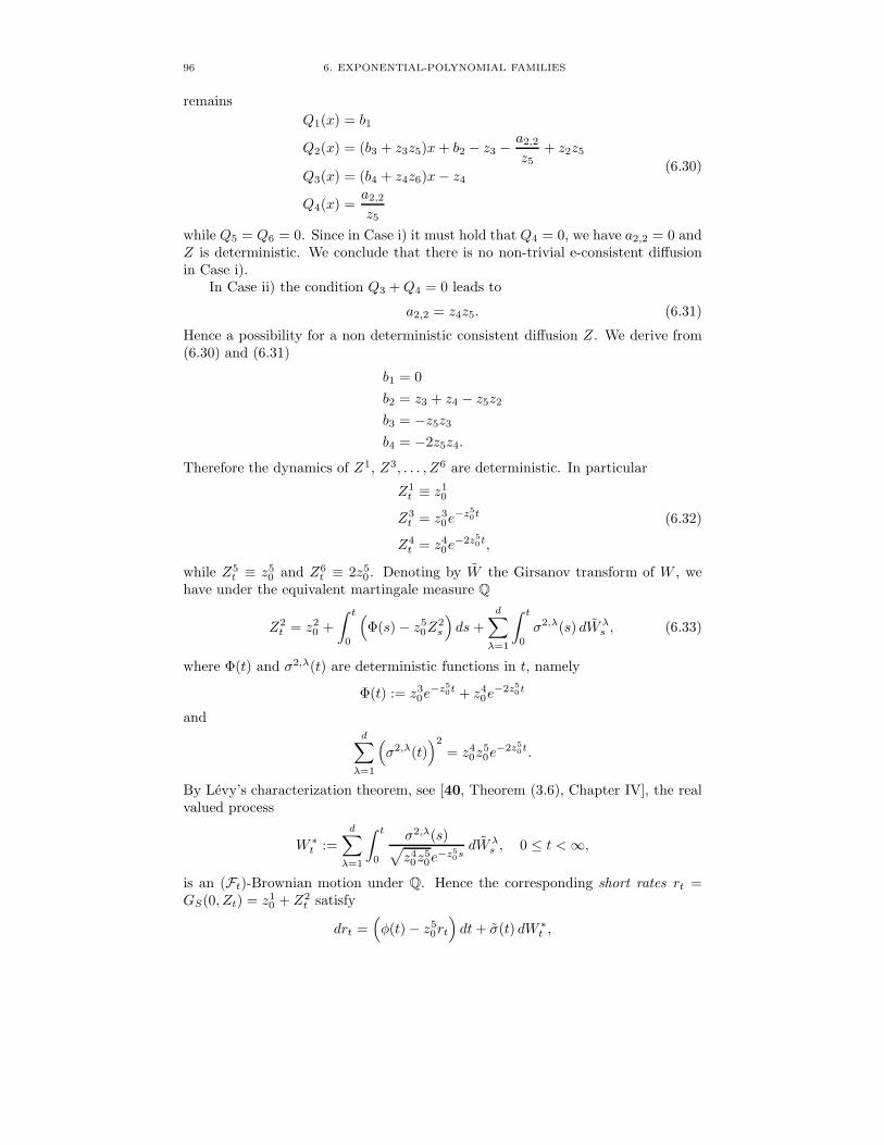
96 6. EXPONENTIAL-POLYNOMIAL FAMILIES
remainsQ1(x) = b1
Q2(x) = (b3 + z3z5)x+ b2 − z3 −a2,2
z5+ z2z5
Q3(x) = (b4 + z4z6)x− z4
Q4(x) =a2,2
z5
(6.30)
while Q5 = Q6 = 0. Since in Case i) it must hold that Q4 = 0, we have a2,2 = 0 andZ is deterministic. We conclude that there is no non-trivial e-consistent diffusionin Case i).
In Case ii) the condition Q3 +Q4 = 0 leads to
a2,2 = z4z5. (6.31)
Hence a possibility for a non deterministic consistent diffusion Z. We derive from(6.30) and (6.31)
b1 = 0b2 = z3 + z4 − z5z2
b3 = −z5z3
b4 = −2z5z4.
Therefore the dynamics of Z1, Z3, . . . , Z6 are deterministic. In particular
Z1t ≡ z1
0
Z3t = z3
0e−z5
0t
Z4t = z4
0e−2z5
0t,
(6.32)
while Z5t ≡ z5
0 and Z6t ≡ 2z5
0 . Denoting by W the Girsanov transform of W , wehave under the equivalent martingale measure Q
Z2t = z2
0 +∫ t
0
(Φ(s)− z5
0Z2s
)ds+
d∑λ=1
∫ t
0
σ2,λ(s) dWλs , (6.33)
where Φ(t) and σ2,λ(t) are deterministic functions in t, namely
Φ(t) := z30e−z5
0t + z40e−2z5
0t
andd∑
λ=1
(σ2,λ(t)
)2
= z40z
50e−2z5
0t.
By Levy’s characterization theorem, see [40, Theorem (3.6), Chapter IV], the realvalued process
W ∗t :=d∑
λ=1
∫ t
0
σ2,λ(s)√z4
0z50e−z5
0sdWλ
s , 0 ≤ t <∞,
is an (Ft)-Brownian motion under Q. Hence the corresponding short rates rt =GS(0, Zt) = z1
0 + Z2t satisfy
drt =(φ(t)− z5
0rt
)dt+ σ(t) dW ∗t ,

6.10. CONCLUSIONS 97
where φ(t) := Φ(t) + z10z
50 and σ(t) :=
√z4
0z50e−z5
0t. This is just the generalizedVasicek model. It can be easily given a closed form solution for rt, see [38, p. 293].
Summarizing Case ii) we have found a non-trivial e-consistent diffusion pro-cess, which is identified by (6.32) and (6.33). Actually Φ has to be replaced bya predictable process Φ due to the change of measure. Nevertheless this is just aone factor model. The corresponding interest rate model is the generalized Vasicekshort rate model. This is very unsatisfactory since Svensson type functions GS(x, z)have six factors z1, . . . , z6 which are observed. And it is seen that after all just oneof them – that is z2 – can be chosen to be non deterministic.
6.10. Conclusions
Bounded exponential-polynomial families like the Nelson–Siegel or Svensson familymay be well suited for daily estimations of the forward rate curve. They are rathernot to be used for inter-temporal interest rate modelling by diffusion processes.This is due to the facts that• the exponents have to be kept constant• and moreover this choice is very restricted
whenever you want to exclude arbitrage possibilities. It is shown for the Nelson–Siegel family in particular that there exists no non-trivial diffusion process providingan arbitrage free model. However there is a choice for the Svensson family, but stilla very limited one, since all parameters but one have to be kept either constant ordeterministic.


CHAPTER 7
Invariant Manifolds for Weak Solutions to
Stochastic Equations
ABSTRACT. Viability and invariance problems related to a stochastic equa-tion in a Hilbert space H are studied. Finite dimensional invariant C2 sub-manifolds of H are characterized. We derive Nagumo type conditions andprove a regularity result: Any weak solution, which is viable in a finite di-mensional C2 submanifold, is a strong solution.
These results are related to finding finite dimensional realizations for sto-chastic equations. There has recently been increased interest in connectionwith a model for the stochastic evolution of forward rate curves.
7.1. Introduction
Consider a stochastic equationdXt = (AXt + F (t,Xt)) dt+B(t,Xt) dWt
X0 = x0(7.1)
on a separable Hilbert space H . Here W denotes a Q-Wiener process on someseparable Hilbert space G. The operator A is the infinitesimal generator of astrongly continuous semigroup in H . The random mappings F = F (t, ω, x) andB = B(t, ω, x) satisfy appropriate measurability conditions.
This paper studies the stochastic viability and invariance problem related toequation (7.1) for finite dimensional regular manifolds in H . A subset M of His called (locally) invariant for (7.1), if for any space-time initial point (t0, x0) ∈R+ ×M any solution X(t0,x0) to (7.1) is (locally) viable in M, i.e. stays (locally)on M almost surely.
Our purpose is to characterize invariant finite dimensional C2 submanifolds Mof H in terms of A, F and B. Under mild conditions on F and B it is shownthat M lies necessarily in the domain D(A) of A. The Nagumo type consistencyconditions
µ(t, ω, x) := Ax + F (t, ω, x)− 12
∑j
DBj(t, ω, x)Bj(t, ω, x) ∈ TxM (7.2)
Bj(t, ω, x) ∈ TxM, ∀j, (7.3)
equivalent to local invariance of M, are derived. Here Bj :=√λjBej , where
λj , ej is an eigensequence defined by Q. If moreover M is closed we can provethat local invariance implies invariance.
The vector fields µ(t, ω, . ) and Bj(t, ω, . ) are shown to be continuous on M.It turns out that the stochastic invariance problem related to (7.1) is equivalent tothe set of deterministic invariance problems related to µ(t, ω, . ) and Bj(t, ω, . ).
99

100 7. INVARIANT MANIFOLDS FOR STOCHASTIC EQUATIONS
By a solution to (7.1) we mean a weak solution, which in contrast to a strongsolution is the natural concept for stochastic equations in Hilbert spaces (see belowfor the exact definitions). It is well known that under some Lipschitz and lineargrowth conditions on F andB, a classical fixed point argument ensures the existenceof a unique weak solution X to (7.1), see [18]. But there is nothing comparablefor the existence of a strong solution, due to the discontinuity of A. However wederive the following regularity result : If dimH < ∞, any linear operator on H iscontinuous and the concepts of a weak and strong solution to (7.1) coincide (atleast if dimG < ∞). We show that this is also true in the general case providedthat X is viable in a finite dimensional C2 submanifold of H .
The main idea behind the proofs is the fact that locally any finite dimensionalsubmanifold M of H can be projected diffeomorphically onto a finite dimensionallinear subspace of D(A?), where A? is the adjoint of A. Thus any weak solutionviable in M is locally mapped onto a finite dimensional semimartingale, whichcan be “pulled back” by Ito’s formula (this is why we assumed M to be C2).This way equation (7.1) is locally transformed into a finite dimensional stochasticequation, which in our setting has a unique strong solution. We use implicitlythat A? restricted to a finite dimensional subset of its domain D(A?) is bounded.Therefore this idea cannot be directly extended to infinite dimensional invariantsubmanifolds.
Many phenomena, say in physics or economics, are described by stochasticequations of the form (7.1). The Hilbert space H is typically a space of functions.Suppose (7.1) represents a stochastic model. Let G := G(·, z) | z ∈ Z be aparametrized family of functions in H , for some parameter set Z ⊂ Rm. Assumethat G is used for statistical estimation of the model coefficients A, F and B in(7.1). That is, one observes the process Z ∈ Z which is related to X by
G(·, Zt) = Xt. (7.4)
The following problems naturally arise:
i) What are the sufficient and necessary conditions on G such that there exists anon-trivial Z-valued process Z satisfying (7.4)? We then say that the modelis consistent with G.
ii) If so, what kind of dynamics does Z inherit from X by (7.4)? (Notice thatX is a priori a weak solution to (7.1), hence not a semimartingale in H .)
If G is regular enough, then G is an m-dimensional C2 submanifold in H . Accord-ingly our results apply: Problem i) is solved by the consistency conditions (7.2) and(7.3). These can be expressed in local coordinates involving the first and secondorder derivatives of G, making them feasible for applications. By our regularityresult, Z is (locally) an Ito process. This responds to Problem ii).
Similar invariance problems have been studied in [7], [10] and [50]. In [7] and[10] the consistency problem for HJM models is solved. However they work withstrong solutions in a Hilbert space, which in general is a rather cutting restriction.In [50] the invariance question for finite dimensional linear subspaces with respect toOrnstein–Uhlenbeck processes is completely solved and applied to various interestrate models. But the methods used in [50] have not yet been established for generalequations (7.1). Therefore our results cannot straightly been obtained that way.
Further recent results can be found in [3], [33] for finite dimensional systems,and in [30], [45] for infinite dimensional ones. See also the references therein.

7.2. PRELIMINARIES ON STOCHASTIC EQUATIONS 101
Compared to these studies we put very mild assumptions on the coefficients of(7.1), which is due to the strong structure of M.
The paper is organized as follows. In Section 7.2 we give the exact setting forequation (7.1) and define (local) weak and strong solutions. Some classical resultson stochastic equations are presented. Section 7.3 contains the main results onstochastic viability and invariance for finite dimensional C2 submanifolds. Theproofs are postponed to Sections 7.4 and 7.5, where we also recall Ito’s formula forour setting. In Section 7.6 we express the consistency conditions (7.2) and (7.3) inlocal coordinates, making them feasible for applications. The appendix includes adetailed discussion on finite dimensional (immersed and regular) submanifolds in aBanach space. Their crucial properties are deduced.
7.2. Preliminaries on Stochastic Equations
For the stochastic background and notations we refer to [18]. We are given a proba-bility space (Ω,F ,P) together with a normal filtration (Ft)0≤t<∞. Let H and G beseparable Hilbert spaces and Q ∈ L(G) a self-adjoint strictly positive operator. SetG0 := Q1/2(G), equipped with the scalar product 〈u, v〉G0 := 〈Q−1/2u,Q−1/2v〉G.We assume W in (7.1) to be a Q-Wiener process on G and Tr Q < ∞. Otherwisethere always exists a separable Hilbert space G1 ⊃ G on which W has a realizationas a finite trace class Wiener process, see [18, Chapt. 4.3].
Denote by L02 := L2(G0;H) the space of Hilbert–Schmidt operators from G0
into H , which itself is a separable Hilbert space. We will focus on the stochasticequation (7.1) under the following set of (standard) assumptions.
• The operator A is the infinitesimal generator of a strongly continuous semi-group in H .• The mappings F and B are measurable from (R+ × Ω ×H,P ⊗ B(H)) into
(H,B(H)), resp. (L02,B(L0
2)).• The initial value is a non random point x0 ∈ H .
Two processes Y and Z are indistinguishable if P[Yt = Zt, ∀t < ∞] = 1. Wewill not distinguish between them.
There is an equivalent way of looking at equation (7.1) which will be usedhere. Let ej be an orthonormal basis of eigenvectors of Q, such that Qej = λjejfor a bounded sequence of strictly positive real numbers λj . Then
√λjej is an
orthonormal basis of G0 and W has the expansion
W =∑j
√λjβ
jej , (7.5)
where βj is a sequence of real independent (Ft)-Brownian motions. This seriesis convergent in the space of G-valued continuous square integrable martingalesM2
T (G), for all T <∞.Recall the following classical result on stochastic integration, see [18, Chapt. 4].
Proposition 7.1. Let E be a separable Hilbert space and σjt be E-valued pre-dictable processes, such that
∑j ‖σ
jt (ω)‖2E <∞ for all (t, ω) ∈ R+ × Ω and
P[ ∫ t
0
∑j
‖σjs‖2E ds <∞]
= 1, ∀t <∞.

102 7. INVARIANT MANIFOLDS FOR STOCHASTIC EQUATIONS
Then the series of stochastic integrals
Mt :=∑j
∫ t
0
σjs dβjs
converges uniformly on compact time intervals in probability. Moreover Mt is anE-valued continuous local martingale and for any bounded stopping time τ
Mt∧τ =∑j
∫ t∧τ
0
σjs dβjs =
∑j
∫ t
0
σjs1[0,τ ](s) dβjs .
Set Bj(t, ω, x) :=√λjB(t, ω, x)ej ∈ H and take into account the identity
‖B(t, ω, x)‖2L02
=∑j
‖Bj(t, ω, x)‖2H <∞. (7.6)
Then equation (7.1) may be equivalently rewritten in the form dXt = (AXt + F (t,Xt)) dt+∑j
Bj(t,Xt) dβjt
X0 = x0.
(7.1′)
Definition 7.2. An H-valued predictable process X is a local weak solutionto (7.1), resp. (7.1’), if there exists a stopping time τ > 0, called the lifetime of X,such that
P[ ∫ t∧τ
0
(‖Xs‖H + ‖F (s,Xs)‖H + ‖B(s,Xs)‖2L0
2
)ds <∞
]= 1, ∀t <∞
and for any t <∞ and ζ ∈ D(A?), P-a.s.
〈ζ,Xt∧τ 〉 = 〈ζ, x0〉+∫ t∧τ
0
(〈A?ζ,Xs〉+ 〈ζ, F (s,Xs)〉
)ds
+∫ t∧τ
0
〈ζ, B(s,Xs) dWs〉,(7.7)
where ∫ t∧τ
0
〈ζ, B(s,Xs) dWs〉 =∑j
∫ t∧τ
0
〈ζ, Bj(s,Xs)〉 dβjs .
A local weak solution X is a local strong solution to (7.1), resp. (7.1’), if in addition
Xt∧τ ∈ D(A), dt⊗ dP-a.s.
P[ ∫ t∧τ
0
‖AXs‖H ds <∞]
= 1, ∀t <∞ (7.8)
and for any t <∞, P-a.s.
Xt∧τ = x0 +∫ t∧τ
0
(AXs + F (s,Xs)
)ds+
∫ t∧τ
0
B(s,Xs) dWs, (7.9)
where ∫ t∧τ
0
B(s,Xs) dWs =∑j
∫ t∧τ
0
Bj(s,Xs) dβjs .
If τ =∞ we just refer to X as weak, resp. strong solution.

7.2. PRELIMINARIES ON STOCHASTIC EQUATIONS 103
This definition may be straightly extended to random F0-measurable initial valuesx0. Notice that the lifetime τ is by no means maximal.
Lemma 7.3. Let X be a weak solution to (7.1) and τ be a bounded stoppingtime. Then Xτ+t is a weak solution to
dYt = (AYt + F (τ + t, Yt)) dt+B(τ + t, Yt) dWt
Y0 = Xτ
(7.10)
with respect to the filtration Ft := Fτ+t, where Wt := Wτ+t −Wτ is a Q-Wienerprocess with respect to Ft. Moreover (7.5) induces the following expansion
W =∑j
√λj β
jej , (7.11)
where βjt := βjτ+t − βjτ is a sequence of real independent (Ft)-Brownian motions.
Proof. First we show that W is a Q-Wiener process with respect to Ft. Ob-viously W0 = 0 and W is continuous and Ft-adapted. Now we proceed as inthe proof of [40, Theorem (3.6), Chapter IV]. Let h ∈ G. Define the functionf ∈ C∞(R+ ×G;C) as follows
f(t, x) := exp(i〈h, x〉G +
t
2〈Qh, h〉G
).
Identify C ∼= R2, then compute
ft(t, x) =12f(t, x)〈Qh, h〉G ∈ L(R;C)
fx(t, x) = if(t, x)〈h, . 〉G ∈ L(H ;C)
fxx(t, x) = −f(t, x)〈h, . 〉G〈h, . 〉G ∈ L(H ×H ;C)
and Ito’s formula, see [18, Chapt 4.5], gives
f(t,Wt) = 1 + i
∫ t
0
f(s,Ws) d〈h,Ws〉G.
Since f(t,Wt) is uniformly bounded on compact time intervals, Mt := f(t,Wt)is a complex martingale (its real and imaginary parts are martingales). By theoptional stopping theorem Mτ+t is a nowhere vanishing complex Ft-martingale.For 0 ≤ s < t <∞
E[Mτ+t
Mτ+s| Fs
]= 1.
Whence for A ∈ Fs we get
E[1A exp(i〈h, Wt − Ws〉G)] = P[A] exp(− 1
2(t− s)〈Qh, h〉G
).
Since this is true for any h ∈ G, the increment Wt − Ws is independent of Fsand has a Gaussian distribution with covariance operator (t − s)Q. Hence W is aQ-Wiener process with respect to Ft.
Next we claim that ∫ τ+t
τ
Φs dWs =∫ t
0
Φτ+s dWs, (7.12)

104 7. INVARIANT MANIFOLDS FOR STOCHASTIC EQUATIONS
for any predictable L02-valued process Φ with
P[ ∫ t
0
‖Φs‖2L02ds <∞
]= 1, ∀t <∞.
If Φ is elementary and τ a simple stopping time, then (7.12) holds by inspec-tion. The general case follows by a well known localization procedure, see [18,Lemma 4.9].
Since X is a weak solution to (7.1), for ζ ∈ D(A?) we thus have
〈ζ,Xτ+t〉 = 〈ζ,Xτ 〉+∫ τ+t
τ
(〈A?ζ,Xs〉+ 〈ζ, F (s,Xs)〉
)ds
+∫ τ+t
τ
〈ζ, B(s,Xs) dWs〉
= 〈ζ,Xτ 〉+∫ t
0
(〈A?ζ,Xτ+s〉+ 〈ζ, F (τ + s,Xτ+s)〉
)ds
+∫ t
0
〈ζ, B(τ + s,Xτ+s) dWs〉.
Hence it follows that Xτ+t is a weak solution to (7.10).
In view of Lemma 7.3 the following definition makes sense.
Definition 7.4. For (t0, x0) ∈ R+×H we denote by X(t0,x0) any (local) weaksolution to
dXt = (AXt + F (t0 + t,Xt)) dt+B(t0 + t,Xt) dW(t0)t
X0 = x0
(7.13)
with respect to the filtration F (t0)t := Ft0+t. Here W
(t0)t := Wt0+t − Wt0 is a
Q-Wiener process with respect to F (t0)t .
All results in this paper for local weak solutions X = X(0,x0) to (7.1) will straightlyapply for local weak solutions X(t0,x0) to (7.13). Hence they are stated only for thecase t0 = 0.
In the sequel we assume X to be a (local) weak solution to (7.1). The mainresults of the next section follow under some regularity assumptions, which forclarity are presented here in a collected form.
(A1): (continuity) There exists a continuous version of X , still denoted by X .(A2): (differentiability) B(t, ω, . ) ∈ C1(H ;L0
2) for all (t, ω) ∈ R+ × Ω.This implies Bj(t, ω, . ) ∈ C1(H ;H), and since
DBj(t, ω, x)Bj(t, ω, x) = (DB(t, ω, x)Bj(t, ω, x))√λjej
hence∑j
‖DBj(t, ω, x)Bj(t, ω, x)‖2H ≤ ‖DB(t, ω, x)‖2L(H;L02)‖B(t, ω, x)‖2L0
2<∞
and∑
j DBj(t, ω, . )Bj(t, ω, . ) ∈ C0(H ;H), for all (t, ω) ∈ R+ × Ω.
(A3): (integrability) For any t <∞ we have
E[ ∫ t
0
(‖Xs‖H + ‖F (s,Xs)‖H + ‖B(s,Xs)‖2L0
2
)ds]<∞.

7.3. INVARIANT MANIFOLDS 105
(A4): (local Lipschitz ) For all T,R < ∞ there exists a real constant C =C(T,R) such that
‖F (t, ω, x)− F (t, ω, y)‖H + ‖B(t, ω, x)−B(t, ω, y)‖L02≤ C‖x− y‖H
for all (t, ω) ∈ [0, T ]× Ω and x, y ∈ H with ‖x‖H ≤ R and ‖y‖H ≤ R.(A5): (right continuity) The mappings F (t, ω, x) and B(t, ω, x) are right con-
tinuous in t, for all x ∈ H and ω ∈ Ω.
Finally we present a classical existence and uniqueness result for local weaksolutions to equation (7.1).
Lemma 7.5. Assume (A4). Then for any x0 there exists a local weak solutionto (7.1) satisfying (A1). Moreover any weak solution to (7.1) satisfying (A1) isunique.
Proof. Let x0 ∈ H . Set l := 2‖x0‖H and define
F (t, ω, x) :=
F (t, ω, x), if ‖x‖H ≤ lF (t, ω, l
‖x‖H x), if ‖x‖H > l
and similarly B(t, ω, x). Then F and B are bounded and globally Lipschitz in x on[0, T ]× Ω×H , for all T <∞. Hence by [18, Theorems 7.4 and 6.5] there exists aunique continuous weak solution X to (7.1), when replacing F by F and B by B.Define the stopping time τ := inft ≥ 0 | ‖X‖H ≥ l. Then τ > 0 and Xt := Xt∧τis a local weak solution to (7.1) with lifetime τ and satisfies (A1).
If X is a continuous weak solution to (7.1) then by the above arguments it isunique on [0, τn] for n ≥ 2, where τn := inft ≥ 0 | ‖X‖H ≥ n‖x0‖H. Now usethat τn ↑ ∞.
7.3. Invariant Manifolds
LetM denote an m-dimensional C2 submanifold of H , m ≥ 1. See the appendix forthe definition and properties of a finite dimensional submanifold in a Hilbert space.The concept of a submanifold is used in more than one sense in the literature, see[11]. We therefore point out that M represents what is also called a regular orembedded submanifold, i.e. the topology and differentiable structure on M is theone induced by H . This allows for deriving global regularity and invariance results,see Theorems 7.6 and 7.7 below.
Essential for our needs is the following observation. Since H is separable, byLindelof’s Lemma [1, p. 4] there exists a countable open covering (Uk)k∈N of Mand for each k a parametrization φk : Vk ⊂ Rm → Uk∩M, where φk ∈ C2
b (Rm;H),see Remark A.8. Using the fact that D(A?) is dense in H , by Proposition A.10 wecan assume that for each k there exists a linearly independent set ζk,1, . . . , ζk,min D(A?) such that
φk(〈ζk,1, x〉, . . . , 〈ζk,m, x〉) = x, ∀x ∈ Uk ∩M. (7.14)
To simplify notation, we write 〈ζk, x〉 instead of (〈ζk,1, x〉, . . . , 〈ζk,m, x〉) and skipthe index k whenever there is no ambiguity.
For the sake of readability all proofs are postponed to the following sections.First we state a (global) regularity result.

106 7. INVARIANT MANIFOLDS FOR STOCHASTIC EQUATIONS
Theorem 7.6. Let X be a local weak solution to (7.1) with lifetime τ , assume(A1) and
Xt∧τ ∈ M, ∀t <∞. (7.15)
Then there exists a stopping time 0 < τ ′ ≤ τ , such that X is a local strong solutionto (7.1) with lifetime τ ′.
If in addition τ =∞ and (A3) holds, then X is a strong solution to (7.1).
We can give sufficient conditions for a weak solution X to be viable in M.Notice that µ(t, ω, x) in (7.2) is well defined by assuming (A2).
Theorem 7.7. Let X be a weak solution to (7.1) with X0 ∈ M. Assume(A1), (A2) and (A4). If M is closed, lies in D(A) and satisfies the consistencyconditions (7.2) and (7.3) for dt ⊗ dP-a.e. (t, ω) ∈ R+ × Ω, for all x ∈ M. Then(7.15) holds for τ =∞.
Moreover A is continuous on M. Consequently (7.2) and (7.3) hold for allx ∈ M, for dt⊗ dP-a.e. (t, ω) ∈ R+ × Ω.
It turns out that the viability condition (7.15) is too weak to imply (7.2) and(7.3). Neither does it imply that M lies in D(A). As a link between Theorems 7.6and 7.7 we shall formulate equivalent conditions for (7.2) and (7.3). Rather thanjust asking for the assumptions of Theorem 7.6 we have to require that (7.15) holdsfor any space-time starting point (t0, x0).
Definition 7.8. The submanifold M is called locally invariant for (7.1), iffor all (t0, x0) ∈ R+ ×M there exists a continuous local weak solution X(t0,x0) to(7.13) with lifetime τ = τ(t0, x0), such that
X(t0,x0)t∧τ ∈ M, ∀t <∞.
Observe that this definition involves local existence.
Theorem 7.9. Assume (A2), (A4) and (A5). Then the following conditionsare equivalent:
i) M is locally invariant for (7.1)ii) M ⊂ D(A) and (7.2), (7.3) hold for dt ⊗ dP-a.e. (t, ω) ∈ R+ × Ω, for all
x ∈ M.iii) M⊂ D(A) and (7.2), (7.3) hold for all (t, x) ∈ R+ ×M, for P-a.e. ω ∈ Ω.
We finally mention the important case whereM is a linear submanifold. Thenthe above results are true under much weaker assumptions.
Theorem 7.10. If M is an m-dimensional linear submanifold, then Theorems7.7 and 7.9 remain valid without assuming (A2) and with µ(t, ω, x) in (7.2) re-placed by
ν(t, ω, x) := Ax + F (t, ω, x).
7.4. Proof of Theorem 7.6
We recall Ito’s formula for our setting.
Lemma 7.11 (Ito’s formula). Assume that we are given the Rm-valued contin-uous adapted process
Yt = Y0 +∫ t
0
bs ds+∑j
∫ t
0
σjs dβjs ,

7.4. PROOF OF THEOREM 7.6 107
where b and σj are Rm-valued predictable processes such that∑j
‖σjt (ω)‖2Rm <∞, ∀(t, ω) ∈ R+ × Ω (7.16)
P[ ∫ t
0
(‖bs‖Rm +
∑j
‖σjs‖2Rm)ds <∞
]= 1, ∀t <∞ (7.17)
and Y0 is F0-measurable. Let φ ∈ C2b (Rm;H). Then Jt := 1
2
∑j D
2φ(Yt)(σjt , σ
jt ) is
an H-valued predictable process,
P[ ∫ t
0
(‖Dφ(Ys)bs‖H +
12
∑j
‖D2φ(Ys)(σjs , σjs)‖H
+∑j
‖Dφ(Ys)σjs‖2H)ds <∞
]= 1, ∀t <∞, (7.18)
and φ Y is a continuous H-valued adapted process given by
(φ Y )t = (φ Y )0 +∫ t
0
(Dφ(Ys)bs + Js
)ds+
∑j
∫ t
0
Dφ(Ys)σjs dβjs . (7.19)
Proof. Point-wise convergence of the series defining Jt follows from (7.16).Hence Jt is predictable. Integrability (7.18) is a direct consequence of (7.17). De-note the right hand side of (7.19) with It. Clearly by (7.18) it is a well definedcontinuous adapted process in H , see Proposition 7.1. Choose an orthonormal ba-sis ei in H . It is enough to show equality (7.19) for each component with respectto ei. Define φi(y) := 〈ei, φ(y)〉. Then φi ∈ C2
b (Rm;R) and Ito’s formula applies,see [18, Theorem 4.17]. It follows
〈ei, (φ Y )t〉 = (φi Y )0 +∫ t
0
(Dφi(Ys)bs +
12
∑j
D2φi(Ys)(σjs, σjs))ds
+∑j
∫ t
0
Dφi(Ys)σjs dβjs
= 〈ei, It〉.
Proof of Theorem 7.6. Assume first that X is a weak solution, that is τ =∞, and that (A3) holds. Fix T > 0. Following [22, Lemma (3.5)] there exists anincreasing sequence of predictable stopping times 0 = T0 ≤ T1 ≤ T2 ≤ · · · ≤ T withsupn Tn = T , such that on each of the intervals
[Tn, Tn+1] ∩ Tn+1 > Tnthe process X takes values in some Uα(n) (here [0, T ] × Tn+1 > Tn is identifiedwith Tn+1 > Tn). This holds due to (A1).
Now let n ∈ N0 and k = α(n). We will analyse X locally on Uk. For simplicitywe shall skip the index k for φk, Uk, Vk and ζk in what follows. Define the Rm-valuedpredictable processes b and σj as
bt := 〈A?ζ,Xt〉+ 〈ζ, F (t,Xt)〉σjt := 〈ζ, Bj(t,Xt)〉,

108 7. INVARIANT MANIFOLDS FOR STOCHASTIC EQUATIONS
where logically 〈A?ζ,Xt〉 stands for (〈A?ζ1, Xt〉, . . . , 〈A?ζm, Xt〉). Then b and σj
satisfy (7.16) and (7.17), see (7.6), and by the very definition of X
Yt := 〈ζ,Xt〉 = 〈ζ, x0〉+∫ t
0
bs ds+∑j
∫ t
0
σjs dβjs .
Hence Ito’s formula (Lemma 7.11) for φ Y applies. Since moreover Y(Tn+t)∧Tn+1
takes values in V on Tn+1 > Tn
X(Tn+t)∧Tn+1 = (φ Y )(Tn+t)∧Tn+1 , on Tn+1 > Tn. (7.20)
Now using (7.7), (7.19) and (7.20) we have for ξ ∈ D(A?)
0 =∫ (Tn+t)∧Tn+1
Tn
(〈A?ξ,Xs〉+ 〈ξ, F (s,Xs)〉
− 〈ξ,Dφ(Ys)bs +12
∑j
D2φ(Ys)(σjs , σjs)〉)ds
+∑j
∫ (Tn+t)∧Tn+1
Tn
(〈ξ, Bj(s,Xs)〉 − 〈ξ,Dφ(Ys)σjs〉
)dβjs .
(7.21)
Notice that the series in the first integral converges point-wise and defines an H-valued predictable process, see Lemma 7.11. By Proposition 7.1 the last termin (7.21) is a continuous local martingale with respect to the filtration (FTn+t).Therefore
〈A?ξ,Xt〉 = 〈ξ,−F (t,Xt) +Dφ(Yt)bt +12
∑j
D2φ(Yt)(σjt , σ
jt )〉 (7.22)
on [Tn, Tn+1]∩Tn+1 > Tn, dt⊗dP-a.s. (see the proof of [25, Proposition 3.2]). Byseparability of H there exists a countable dense subset D ⊂ D(A?) such that (7.22)holds simultaneously for all ξ ∈ D and for all (t, ω) ∈ [Tn, Tn+1] ∩ Tn+1 > Tnoutside an exceptional dt⊗ dP-nullset. Let (t, ω) be such a point of validity. Then〈A?ξ,Xt(ω)〉 is a linear functional on D(A?), which is bounded on D by (7.22).Hence it is bounded and therefore continuous on D(A?). Since A?? = A, see [41,Theorem 13.12], we conclude that Xt(ω) ∈ D(A) and – using full notation again –
AXt + F (t,Xt) = Dφ(Yt)(〈A?ζ,Xt〉+ 〈ζ, F (t,Xt)〉
)+
12
∑j
D2φ(Yt)(〈ζ, Bj(t,Xt)〉, 〈ζ, Bj(t,Xt)〉)(7.23)
on [Tn, Tn+1] ∩ Tn+1 > Tn, dt⊗ dP-a.s.Similarly one shows that (compute the quadratic covariation of (7.21) with βj)
Bj(t,Xt) = Dφ(Yt)〈ζ, Bj(t,Xt)〉, ∀j, (7.24)
on [Tn, Tn+1] ∩ Tn+1 > Tn, dt⊗ dP-a.s.

7.4. PROOF OF THEOREM 7.6 109
In view of (A3)
E[ ∫ T
0
(‖Dφ(Ys)bs‖H +
12
∑j
‖D2φ(Ys)(σjs , σjs)‖H +
∑j
‖Dφ(Ys)σjs‖2H)ds]
≤ C1E[ ∫ T
0
(‖bs‖Rm +
∑j
‖σjs‖2Rm)ds]
≤ C2E[ ∫ T
0
(‖Xs‖H + ‖F (s,Xs)‖H + ‖B(s,Xs)‖2L0
2
)ds]<∞,
(7.25)
where C1 and C2 depend only on n.Summing up over 0 ≤ n ≤ N − 1 we get from (7.23) and (7.25)
E[ ∫ TN
0
‖AXs‖H ds]<∞, ∀N ∈ N.
Since limN ↑ TN = T
P[ ∫ t
0
‖AXs‖H ds <∞]
= 1, ∀t < T,
and by the identities (7.23) and (7.24)
Xt = x0 +∫ t
0
(AXs + F (s,Xs)) ds+∑j
∫ t
0
Bj(s,Xs) dβjs .
Since T was arbitrary the second part of the theorem is proved.Now assume X to be a local weak solution with lifetime τ . Let φ : V → U ∩M
be a parametrization in X0 satisfying (7.14). By (A1) there exists a stopping timeT1 > 0, such that Xt∧τ takes values in U on [0, T1]. Set τ ′ := τ ∧ T1.
The rest of the proof runs as before, only estimation (7.25) has to be replaced.We give a sketch. Define
bt :=(〈A?ζ,Xt∧τ ′〉+ 〈ζ, F (t,Xt∧τ ′)〉
)1[0,τ ′](t)
σjt := 〈ζ, Bj(t,Xt∧τ ′)〉1[0,τ ′](t).
Then
Xt∧τ ′ = (φ Y )t, ∀t <∞ (7.26)
where
Yt := 〈ζ,Xt∧τ ′〉 = 〈ζ, x0〉+∫ t
0
bs ds+∑j
∫ t
0
σjs dβjs . (7.27)
Instead of (7.25) we now have (7.17) by the very definition of X . Using (7.26) andLemma 7.11 we get the relations (7.23) and (7.24) for X on [0, τ ′], dt⊗ dP-a.s. Inparticular Xt∧τ ′ ∈ D(A), dt⊗ dP-a.s. Hence from (7.18) and (7.23) we derive (7.8)and (7.9).

110 7. INVARIANT MANIFOLDS FOR STOCHASTIC EQUATIONS
7.5. Proof of Theorems 7.7, 7.9 and 7.10
A key step in proving Theorems 7.7, 7.9 and 7.10 consists in the following property.
Lemma 7.12. Assume (A2) and (A4). Let φ : V → U ∩M be a parametriza-tion satisfying (7.14). Suppose that U ∩M ⊂ D(A). Then (7.2) and (7.3) hold fordt⊗ dP-a.e. (t, ω) ∈ R+ × Ω, for all x ∈ U ∩M if and only if
Ax+ F (t, ω, x) = Dφ(y)(〈A?ζ, x〉 + 〈ζ, F (t, ω, x)〉
)+
12
∑j
D2φ(y)(〈ζ, Bj(t, ω, x)〉, 〈ζ, Bj(t, ω, x)〉) (7.28)
Bj(t, ω, x) = Dφ(y)〈ζ, Bj(t, ω, x)〉, ∀j, (7.29)
where y = 〈ζ, x〉, for all x ∈ U ∩M, for dt⊗ dP-a.e. (t, ω) ∈ R+ × Ω.Consequently A is contiuous on U ∩M.
Proof. Point-wise equivalence of (7.3) and (7.29), and of (7.2) and the relation
Ax+ F (t, ω, x)− 12
∑j
DBj(t, ω, x)Bj(t, ω, x)
= Dφ(y)〈ζ, Ax + F (t, ω, x)− 12
∑j
DBj(t, ω, x)Bj(t, ω, x)〉 (7.30)
follows from Lemma A.11. Assume (7.2) and (7.3) – and hence (7.29) and (7.30) –hold for dt ⊗ dP-a.e. (t, ω) ∈ R+ × Ω, for all x ∈ U ∩M. But both sides of (7.29)are continuous in x by (A2). Hence there exists a dt ⊗ dP-nullset N ⊂ R+ × Ω,such that (7.29) is true simoultaneously for all x ∈ U ∩M and (t, ω) ∈ N c.
Fix (t, ω) ∈ N c. In view of (A2) Proposition A.12 applies and the last sum-mand in (7.28) equals
12
∑j
DBj(t, ω, x)Bj(t, ω, x)− 12Dφ(y)〈ζ,
∑j
DBj(t, ω, x)Bj(t, ω, x)〉.
Hence (7.28) holds for (t, ω, x) ∈ N c × (U ∩M) if and only if (7.30) does so.It remains to show validity of (7.28) for all x ∈ U ∩M, for dt⊗ dP-a.e. (t, ω).
We abbreviate the right hand side of (7.28) to R(t, ω, x). Then it reads
Ax = −F (t, ω, x) +R(t, ω, x) (7.31)
for dt ⊗ dP-a.e. (t, ω), for all x ∈ U ∩M. But due to (A4) the right hand side of(7.31) is continuous in x, see (7.6). Hence for any (countable) sequence xn → x inU ∩M we have Axn → Ax, by the closedness of A. In other words A restricted toU ∩M is continuous. This establishes the lemma.
Proof of Theorem 7.7. Define the stopping time τ0 := inft ≥ 0 | Xt /∈M. By closedness of M and (A1) we have Xτ0 ∈ M on τ0 < ∞. We claimτ0 =∞.
Assume P[τ0 < K] > 0 for a number K ∈ N. By countability of the cov-ering (Uk) there exists a parametrization φ : V → U ∩M, satisfying (7.14) andP[Xτ0 ∈ U and τ0 < K] > 0. Define the bounded stopping time τ1 := τ0 ∧K and

7.5. PROOF OF THEOREMS 7.7, 7.9 AND 7.10 111
set Y0 := 〈ζ,Xτ1〉. Since φ ∈ C2b (Rm;H), the Rm-valued, resp. L2(G0;Rm)-valued
mappings
b(t, ω, y) := 〈A?ζ, φ(y)〉 + 〈ζ, F (τ1(ω) + t, ω, φ(y))〉σ(t, ω, y) := 〈ζ, B(τ1(ω) + t, ω, φ(y))( . )〉σj(t, ω, y) :=
√λjσ(t, ω, y)ej = 〈ζ, Bj(τ1(ω) + t, ω, φ(y))〉
are bounded and globally Lipschitz in y on [0, T ]×Ω×Rm for all T <∞, which isdue to (A4). By Lemma 7.3 the process Wt := Wτ1+t−Wτ1 is a Q-Wiener processexpanded by βjt given by (7.11). Hence the stochastic differential equation in Rm
Yt = Y0 +∫ t
0
b(s, Ys) ds+∑j
∫ t
0
σj(s, Ys) dβjs (7.32)
has a unique continuous strong solution Y , see [18, Theorem 7.4].Now P[Y0 ∈ V | τ0 < K] · P[τ0 < K] = P[Y0 ∈ V and τ0 < K] > 0 and the dis-
tribution of Y0 under P[ . | τ0 < K] is regular. Hence by normality of Rm there existstwo open sets V0, V1 such that V 0 ⊂ V1 ⊂ V 1 ⊂ V and P[Y0 ∈ V 0 and τ0 < K] > 0.Define the (Ft)-stopping time
τ2 :=
inft ≥ 0 | Yt /∈ V1, if Y0 ∈ V 0 and τ0 < K
0, otherwise.(7.33)
Then by continuity of Y we have P[τ2 > 0] = P[Y0 ∈ V 0 and τ0 < K] > 0 and
Y ∈ V on [0, τ2] ∩ τ2 > 0. (7.34)
From the boundedness of b and σ we derive
E[ ∫ t
0
(‖b(s, Ys)‖Rm +
∑j
‖σj(s, Ys)‖2Rm)ds]<∞, ∀t <∞. (7.35)
Set X := φ Y . The assumptions of Lemma 7.11 are satisfied, hence
Xt = Xτ1 +∫ t
0
(Dφ(Ys)b(s, Ys) +
12
∑j
D2φ(Ys)(σj(s, Ys), σj(s, Ys)))ds
+∑j
∫ t
0
Dφ(Ys)σj(s, Ys) dβjs , on [0, τ2] ∩ τ2 > 0,(7.36)
where the series in the first integral converges point-wise and defines an H-valuedpredictable process. Moreover by (7.34) we have
X ∈ (U ∩M) ⊂ D(A) on [0, τ2] ∩ τ2 > 0. (7.37)
Hence due to (A2) and (A4) Lemma 7.12 applies and
AXt + F (τ1 + t, Xt) = Dφ(Yt)b(t, Yt) +12
∑j
D2φ(Yt)(σj(t, Yt), σj(t, Yt))
Bj(τ1 + t, Xt) = Dφ(Yt)σj(t, Yt), ∀j,

112 7. INVARIANT MANIFOLDS FOR STOCHASTIC EQUATIONS
on [0, τ2] ∩ τ2 > 0, dt⊗ dP-a.s. This together with (7.35) and (7.36) implies
P[ ∫ t∧τ2
0
‖AXs‖H ds <∞]
= 1, ∀t <∞
Xt∧τ2 = Xτ1 +∫ t∧τ2
0
(AXs + F (τ1 + s, Xs)
)ds+
∑j
∫ t∧τ2
0
Bj(τ1 + s, Xs) dβjs ,
on τ2 > 0. On the other hand we know by Lemmas 7.3 and 7.5 that Xτ1+t is theunique continuous weak solution to dZt = (AZt + F (τ1 + t, Zt)) dt+
∑j
Bj(τ1 + t, Zt) dβj t
Z0 = Xτ1
Whence Xt = Xτ1+t on [0, τ2] ∩ τ2 > 0. Because of (7.37) in particular Xτ1+τ2 ∈M. But by construction τ0 < K = τ0 < K ∩ τ0 = τ1 and
0 < P[τ2 > 0] ≤ P[τ1 + τ2 > τ1 ∩ τ0 < K] ≤ P[τ1 + τ2 > τ0],
which is absurd. Hence τ0 =∞.The last statement of the theorem follows from Lemma 7.12 and (A2).
Proof of Theorem 7.9. i)⇒ii): Fix (t0, x0) ∈ R+ ×M and denote by X =X(t0,x0) a continuous local weak solution to (7.13) with lifetime τ . We proceedas in the proof of Theorem 7.6 and adapt the notation. Define the F (t0)
t -stoppingtime T1 > 0 with the property that Xt∧τ ′ takes values in Uα(0) for τ ′ := τ ∧ T1.Analogously to (7.22) we derive the equality
〈A?ξ,Xt〉 =⟨ξ,− F (t0 + t,Xt) +Dφ(Yt)
(〈A?ζ,Xt〉+ 〈ζ, F (t0 + t,Xt)〉
)+
12
∑j
D2φ(Yt)(〈ζ, Bj(t0 + t,Xt)〉, 〈ζ, Bj(t0 + t,Xt)〉)⟩,
(7.38)
for all ξ ∈ D(A?) on [0, τ ′], dt⊗dP-a.s. Due to (A4) and (A5) both sides of (7.38)are right continuous in t. Hence for P-a.e. ω the limit t ↓ 0 exists. By (7.6) we caninterchange the limiting t ↓ 0 with the summation over j. Arguing as for (7.23) weconclude that x0 ∈ D(A) and
Ax0 + F (t0, ω, x0) = Dφ(y0)(〈A?ζ, x0〉+ 〈ζ, F (t0, ω, x0)〉
)+
12
∑j
D2φ(y0)(〈ζ, Bj(t0, ω, x0)〉, 〈ζ, Bj(t0, ω, x0)〉), P-a.s.
Similarly
Bj(t0, ω, x0) = Dφ(y0)〈ζ, Bj(t0, ω, x0)〉, ∀j, P-a.s.
Since (t0, x0) was arbitrary, Lemma 7.12 yields condition ii).ii)⇒i): Let (t0, x0) ∈ R+ ×M and let φ : V → U ∩M be a parametrization in
x0 satisfying (7.14). As in the proof of Theorem 7.7 (setting τ0 = τ1 = 0) we get a

7.6. CONSISTENCY CONDITIONS IN LOCAL COORDINATES 113
unique continuous strong solution Y to
Yt = 〈ζ, x0〉+∫ t
0
(〈A?ζ, φ(Ys)〉+ 〈ζ, F (t0 + s, φ(Ys))〉
)ds
+∑j
∫ t
0
〈ζ, Bj(t0 + s, φ(Ys))〉 dβ(t0),js .
Here β(t0),jt := βjt0+t − β
jt0 is the sequence of (F (t0)
t )-Brownian motions related toW
(t0)t by (7.11). The stopping time τ2 given by (7.33) is strictly positive and Yt∧τ2 ∈
V . Analysis similar to that in the proof of Theorem 7.7 shows that X(t0,x0)t :=
(φ Y )t∧τ2 is a continuous local strong solution to (7.13) with lifetime τ2 andX
(t0,x0)t ∈ U ∩M, for all t <∞.
ii)⇔iii): This is a direct consequence of Lemma 7.12 and (A5).
Proof of Theorem 7.10. In view of Proposition A.10 we can choose anyparametrization φk in (7.14) such that D2φk ≡ 0 on Vk. By straightforward in-spection of the proofs we see that Lemma 7.12 and Theorems 7.7 and 7.9 remainvalid under the conditions stated in the theorem.
7.6. Consistency Conditions in Local Coordinates
In this section we express the consistency conditions (7.2) and (7.3) in local co-ordinates and identify the underlying coordinate process Y . From now on theassumptions of Theorem 7.9 are in force andM is locally invariant for (7.1).
Let φ : V → U ∩M be a parametrization. We assume that (A.1) and (A.2)hold for all y ∈ V (otherwise replace V by V ∩ V ′). Consequently
‖Dφ(y)−1‖L(Tφ(y)M;Rm) ≤ ‖DΨ(φ(y))‖, ∀y ∈ V (7.39)
and the latter is locally bounded since Ψ is C2. Theorem 7.9 says that
µ(t, ω, φ(y)) = Dφ(y)b(t, ω, y) (7.40)
Bj(t, ω, φ(y)) = Dφ(y)ρj(t, ω, y), ∀j, (7.41)
for all (t, ω, y) ∈ R+ × Ω × V (after removing a P-nullset from Ω), where b andρj are uniquely specified mappings measurable from (R+ × Ω× V,P ⊗ B(V )) into(Rm,B(Rm)), see (A.3). By (7.39)
ρ(t, ω, y) := Dφ(y)−1B(t, ω, φ(y))(·) ∈ L2(G0;Rm).
To simplify notation, we suppress the argument ω whenever there is no ambiguity.In view of (A2) and (A.2), ρj(t, ·) ∈ C1(V ;Rm).
Fix (t, y) ∈ V . It is shown at the end of the appendix that
DBj(t, φ(y))Bj(t, φ(y)) =d
dsBj(t, c(s))|s=0
where c(s) := φ(y + sρj(t, y)). On the other hand, by (7.41)
d
dsBj(t, c(s))|s=0 =
d
ds
(Dφ(y + sρj(t, y))ρj(t, y + sρj(t, y))
)|s=0
= D2φ(y)(ρj(t, y), ρj(t, y)
)+Dφ(y)
(Dρj(t, y)ρj(t, y)
),

114 7. INVARIANT MANIFOLDS FOR STOCHASTIC EQUATIONS
compare with (A.7). Inserting this in (7.40) yields
Aφ(y) + F (t, φ(y)) − 12
∑j
D2φ(y)(ρj(t, y), ρj(t, y)
)= Dφ(y)b(t, y), (7.42)
where b(t, ω, y) := b(t, ω, y) + 12
∑j Dρ
j(t, ω, y)ρj(t, ω, y). By (7.6), (7.39) and(A2), the series converge absolutely and are continuous in y.
We now show how equation (7.13) can be written in local coordinates. Weclaim that b(t, ω, y) ∈ Rm and ρ(t, ω, y) are locally Lipschitz in y on [0, T ]×Ω×V ,for all T <∞. Indeed, the right hand side of (7.28) is locally Lipschitz in y by (A4)and hence also the left hand side of (7.42), see (7.6) and (7.39). Solving (7.42) forb yields the claim.
Consequently, for any (t0, y0) ∈ R+ × V there exists by [18, Theorem 7.4] aunique continuous local strong solution Y (t0,y0) ∈ V to dYt = b(t0 + t, Yt) dt+
∑j
ρj(t0 + t, Yt) dβ(t0),jt
Y0 = y0
(7.43)
with lifetime τ(t0, y0), where β(t0),jt := βjt0+t − β
jt0 , see (7.11). Using Ito’s formula
(Lemma 7.11) and proceeding as in the proof of Theorem 7.7, we see that
X(t0,x0)t := (φ Y (t0,y0))t∧τ(t0,y0)
is the unique continuous local strong solution to (7.13) with lifetime τ(t0, y0), wherex0 = φ(y0).
Summarizing, we have proved
Theorem 7.13. Under the above assumptions, the consistency conditions (7.2)and (7.3) hold for all (t, ω, x) ∈ R+×Ω× (U ∩M) if and only if (7.42) and (7.41)hold for all (t, ω, y) ∈ R+ × Ω× V .
The coefficients b and ρ are locally Lipschitz continuous in y ∈ V : For anyT,R ∈ R+ there exists a real constant C = C(T,R) such that
‖b(t, ω, y)− b(t, ω, z)‖Rm + ‖ρ(t, ω, y)− ρ(t, ω, z)‖L2(G0;Rm) ≤ C‖y − z‖Rm (7.44)
for all (t, ω) ∈ [0, T ]× Ω and y, z ∈ V ∩BR(Rm).Moreover equation (7.13) transforms locally into equation (7.43). That is,
X(t0,x0) is a continuous local strong solution to (7.13) in U ∩ M if and only ifso is φ−1 X(t0,x0) to (7.43) in V , where y0 = φ−1(x0).
If φ is linear (D2φ ≡ 0), then the same holds true without assuming (A2).

Appendix: Finite Dimensional Submanifolds in
Banach Spaces
For the convenience of the reader we discuss and prove some crucial propertiesof finite dimensional submanifolds in Banach spaces. The main tool from infinitedimensional analysis is the inverse mapping theorem, see [1, Theorem 2.5.2], whichdoes not rely on a scalar product. Therefore we chose this somewhat oversizedframework, although in our setting stochastic equations take place in Hilbert spaces.
Let E denote a Banach space, E′ it’s dual space. We write 〈e′, e〉 for the dualitypairing. For a direct sum decomposition E = E1 ⊕ E2 we denote by Π(E2,E1) theinduced projection onto E1.
Let k,m ∈ N. We begin with an important corollary of the inverse mappingtheorem, see [1, Theorem 2.5.12].
Proposition A.1. Let φ ∈ Ck(V ;E), for some open set V ⊂ Rm. SupposeDφ(y0) is one to one for some y0 ∈ V . Then Dφ(y0)Rm is m-dimensional andcomplemented in E
E = Dφ(y0)Rm ⊕ E2.
Moreover, there exist two open neighborhoods V ′ of (y0, 0) in V ×E2 and U of φ(y0)in E, and a Ck diffeomorphism Ψ : U → V ′ such that
Ψ φ(y) = (y, 0), ∀y ∈ V ′ ∩ (Rm × 0). (A.1)
Furthermore, Dφ(y) is one to one and
Dφ(y)−1 = DΨ(φ(y))|Dφ(y)Rm , ∀y ∈ V ′ ∩ (Rm × 0). (A.2)
Proof. Let e1, . . . , em be a basis of Dφ(y0)Rm. Every z ∈ Dφ(y0)Rm hasa unique representation z = z1e1 + . . . zmem. Set αi(z) := zi. Each αi extends toa member e′i of E′ by the Hahn–Banach theorem. Define E2 as the intersectionof the null spaces of all e′i. Then E = Dφ(y0)Rm ⊕ E2 and Π(E2,Dφ(y0)Rm) =〈e′1, ·〉e1 + . . . 〈e′m, ·〉em.
Define Φ : V × E2 → E by Φ(y, z) := φ(y) + z. Then Φ ∈ Ck(V × E2;E)and DΦ(y, z)(v1, v2) = Dφ(y)v1 + v2 for (v1, v2) ∈ Rm × E2, see [1, Prop. 2.4.12].Now DΦ(y0, 0) : Rm × E2 → E is linear, bijective and continuous, hence a linearisomorphism by the open mapping theorem. Accordingly, the inverse mappingtheorem yields the existence of U and V ′ as claimed such that Φ : V ′ → U is a Ck
diffeomorphism with inverse Ψ.Consequently, Ψ φ(y) = Ψ Φ(y, 0) = (y, 0) for y ∈ V ′ ∩ (Rm × 0). The
chain rule gives DΨ(φ(y))Dφ(y) = IdRm . Hence Dφ(y) is one to one and (A.2)holds.
115

116 APPENDIX: FINITE DIMENSIONAL SUBMANIFOLDS IN BANACH SPACES
Definition A.2. The mapping φ from Proposition A.1 is called a Ck immer-sion at y0. If φ is a Ck immersion at each y0 ∈ V , we just say φ is a Ck immersion.
If φ : V → E is an injective Ck immersion, V ⊂ Rm open, we call M := φ(V )an m-dimensional immersed Ck submanifold of E.
The next definition straightly extends the concept of a regular surface in R3.
Definition A.3. A subsetM⊂ E is an m-dimensional (regular) Ck subman-ifold of E, if for all x ∈ M there is a neighborhood U in E, an open set V ⊂ Rmand a Ck map φ : V → E such that
i) φ : V → U ∩M is a homeomorphismii) Dφ(y) is one to one for all y ∈ V .
The map φ is called a parametrization in x.M is a linear submanifold if for all x ∈M there exists a linear parametrization
of the form φ(y) = x+∑m
i=1 yiei in x.
Let φ : V → E be an injective Ck immersion, V ⊂ Rm open, whenceM = φ(V )an immersed submanifold. In the notation of Proposition A.1 we have by (A.1)that φ : V ′ ∩ (Rm × 0) → φ(V ′ ∩ (Rm × 0)) is a homeomorphism, and henceφ(V ′ ∩ (Rm × 0)) is a regular submanifold. Yet in general φ : V → M is not ahomeomorphism. In other words, being an immersed submanifold does not implybeing a regular submanifold. This is the crucial difference between an immersionand an embedding. For examples and more details see [1, Section 3.5].
In what follows, M denotes an m-dimensional Ck submanifold of E. As animmediate consequence of Proposition A.1 and Definition A.3 we show that Mshares in fact the characterizing property of a Ck manifold:
Lemma A.4. Let φi : Vi → Ui ∩M, i = 1, 2, be two parametrizations such thatW := U1 ∩ U2 ∩M 6= ∅. Then the change of parameters
φ−11 φ2 : φ−1
2 (W )→ φ−11 (W )
is a Ck diffeomorphism.
Proof. Of course, φ−11 φ2 : φ−1
2 (W )→ φ−11 (W ) is a homeomorphism.
Now let y ∈ φ−12 (W ) and r = φ−1
1 φ2(y). Then E = Dφ1(r)Rm ⊕ E2 byProposition A.1. Moreover there exist two open neighborhoods V ′1 ⊂ V1 × E2 of(r, 0) and U ′ ⊂ E of φ1(r), and a Ck diffeomorphism Ψ : U ′ → V ′1 such thatφ1 = Ψ−1 on V ′1 ∩ (Rm × 0).
Now again we use the fact that φ1 is a homeomorphism. Hence there existsan open set U ′′ ⊂ E with φ1(V ′1 ∩ (Rm × 0)) = U ′′ ∩ M. Set U := U ′ ∩ U ′′.Then φ−1
1 = Ψ on U ∩ M. By continuity of φ2 there is an open neighborhoodV ′2 ⊂ φ−1
2 (W ) of y with φ2(V ′2 ) ⊂ U ∩M. But then φ−11 φ2|V ′2 = Ψ φ2|V ′2 is Ck
in V ′2 .Since y was arbitrary, φ−1
1 φ2 is Ck in φ−12 (W ). By symmetry the assertion
follows.
Definition A.5. For x ∈ M the tangent space to M at x is the subspace
TxM := Dφ(y)Rm, y = φ−1(x),
where φ : V ⊂ Rm →M is a parametrization in x.

APPENDIX: FINITE DIMENSIONAL SUBMANIFOLDS IN BANACH SPACES 117
By Lemma A.4, the definition of TxM is independent of the choice of the para-metrization.
Definition A.6. A vector field X on M is a mapping assigning to each pointx of M an element X(x) of TxM.
A vector field X can be represented locally as
X(x) = Dφ(y)α(y), y = φ−1(x), ∀x ∈ U ∩M, (A.3)
where φ : V → U ∩M is a parametrization and α is an Rm-valued vector field onV (uniquely determined by φ). This is how smoothness of vector fields on M canbe defined in terms of smoothness of Rm-valued vector fields.
Definition A.7. The vector field X is of class Cr, 0 ≤ r < k, if for anyparametrization φ the corresponding Rm-valued vector field α in (A.3) is of classCr.
Again by Lemma A.4 this is a well defined concept.It will be useful to extend a parametrization to the whole of Rm. Let x ∈ M
and φ : V → U ∩ M be a parametrization in x. Set y = φ−1(x). Since V is aneighborhood of y there exists ε > 0 such that the open ball
B2ε(y) := v ∈ Rm | |y − v| < 2ε
is contained in V . On B2ε(y) one can define a function ψ ∈ C∞(Rm; [0, 1]) satisfyingψ ≡ 1 on Bε(y) and supp(ψ) ⊂ B2ε(y), see [11, Theorem (5.1), Chapt. II]. Since φ isa homeomorphism there exists an open neighborhood U ′ of x in E with φ(Bε(y)) =U ′∩M. Set φ := ψφ. Then φ ∈ Ckb (Rm;E) and φ|Bε(y) = φ|Bε(y) : Bε(y)→ U ′∩Mis a parametrization in x. We have thus shown
Remark A.8. We may and will assume that any parametrization φ : V →U ∩M extends to φ ∈ Ckb (Rm;E).
Let x ∈ M. As shown in Proposition A.1, the tangent space TxM is com-plemented in E by E2 = ∩mi=1N (e′i), where e1, . . . , em is a basis for TxM and〈e′i, ej〉 = δij (Kronecker delta). The following lemma states that, locally in x,Π(E2,TxM) is a diffeomorphism on M into TxM.
Lemma A.9. There exists a parametrization φ : V → U ∩M in x such that
φ(〈e′1, z〉, . . . , 〈e′m, z〉) = z, ∀z ∈ U ∩M.
Proof. Let ψ : V1 → U1 ∩ M be a parametrization in x and write y =ψ−1(x). Denote by ITxM : TxM → Rm the canonical isomorphism ITxM :=(〈e′1, ·〉, . . . , 〈e′m, ·〉). Then the map h := ITxM Π(E2,TxM) ψ : V1 → Rm is Ck andDh(y) = ITxM Dψ(y) is one to one. By the inverse mapping theorem there existopen neighborhoods W ⊂ V1 of y and V ⊂ Rm of h(y) such that h : W → V is aCk diffeomorphism. Since ψ is a homeomorphism there is an open neighborhoodU ⊂ E of x with ψ(W ) = U ∩M. The map φ := ψ h−1 : V → U ∩M is then thedesired parametrization in x, that is, φ−1 = ITxM Π(E2,TxM) on U ∩M.
The following result is crucial for our discussion on weak solutions to stochasticequations viable in M.

118 APPENDIX: FINITE DIMENSIONAL SUBMANIFOLDS IN BANACH SPACES
Proposition A.10. Let D ⊂ E′ be a dense subset. Then for any x ∈M thereexist elements f ′1, . . . , f ′m in D and a parametrization φ : V → U ∩M in x suchthat
φ(〈f ′1, z〉, . . . , 〈f ′m, z〉) = z, ∀z ∈ U ∩M.
If M is linear, then φ is linear: φ(v) = e0 +∑mi=1(
∑mj=1 Nijvj)ei, for v ∈ V .
Proof. The idea is to find a decomposition E = F1 ⊕ F2, dimF1 = m, suchthat F1 is “not too far” from TxM and such that Π(F2,F1) = 〈f ′1, ·〉f1 + · · · +〈f ′m, ·〉fm, with f ′1 . . . , f
′m ∈ D. Thereby the expression “not too far” means that
Π(F2,F1)|TxM : TxM→ F1 is an isomorphism.Let e1, . . . , em be a basis for TxM and ψ : V1 → U1∩M the parametrization
in x given by Lemma A.9. Set y = ψ−1(x). We may assume that ‖ei‖E = 1, for1 ≤ i ≤ m. Since D is dense in E′, there exist elements f ′1, . . . , f
′m in D with
‖f ′i − e′i‖E′ < 2−m. Notice that by definition 〈e′i, ej〉 = δij . Hence
|〈f ′i , ej〉| ≤ |〈e′i, ej〉|+ |〈f ′i − e′i, ej〉| < 2−m, if i 6= j
and
|〈f ′i , ei〉| ≥ |〈e′i, ei〉| − |〈f ′i − e′i, ei〉| > 1− 2−m.
The matrix M := (〈f ′i , ej〉)1≤i,j≤m is therefore invertible, which follows from thetheorem of Gerschgorin, see [43]. Consequently, the family f ′1, . . . , f ′m is linearlyindependent in E′. Since E is reflexive, by the Hahn–Banach theorem there existsa linearly independent set f1, . . . , fm in E such that 〈f ′i , fj〉 = δij . Write F1 :=spanf1, . . . , fm. The f ′i and fi induce then a decomposition E = F1 ⊕ F2 withprojection Π(F2,F1) = 〈f ′1, ·〉f1 + · · ·+ 〈f ′m, ·〉fm. Since
Π(F2,F1)ej =m∑i=1
Mijfi, for 1 ≤ j ≤ m,
we see that Π(F2,F1)|TxM : TxM → F1 is an isomorphism. Let IF1 : F1 → Rmdenote the canonical isomorphism IF1 := (〈f ′1, ·〉, . . . , 〈f ′m, ·〉). Then the map h :=IF1 Π(F2,F1) ψ : V1 → Rm is Ck and Dh(y) = IF1 Π(F2,F1) Dψ(y) is one toone. Now proceed as in the proof of Lemma A.9 to get the desired parametrizationφ in x with φ−1 = IF1 Π(F2,F1) on U ∩M, for some neighborhood U of x.
If M is linear, we choose ψ(u) = x +∑mi=1 uiei. An easy computation shows
that φ(v) = (x − (Π(F2,F1)|TxM)−1 Π(F2,F1)x) +∑mi=1(
∑mj=1 M
−1ij vj)ei. Setting
N := M−1 and e0 := x− (Π(F2,F1)|TxM)−1 Π(F2,F1)x completes the proof.
Lemma A.9 asserts the existence of a particular parametrization φ : V →U ∩M in x ∈ M related to the decomposition E = TxM⊕ E2. Actually, E2 iscomplemented in E simultaneously by all tangent spaces TzM, z ∈ U ∩M.
Lemma A.11. Let φ : V → U ∩M be a parametrization. If there exist elementse′1, . . . , e
′m in E′ with the property that
φ(〈e′1, x〉, . . . , 〈e′m, x〉) = x, ∀x ∈ U ∩M,
then e′1, . . . , e′m are linearly independent in E′ and
E = TxM⊕ E2, ∀x ∈ U ∩M,
where E2 :=⋂mi=1N (e′i). Moreover, the induced projections are given by
Π(E2,TxM) = Dφ(y)(〈e′1, ·〉, . . . , 〈e′m, ·〉), y = φ−1(x), ∀x ∈ U ∩M. (A.4)

APPENDIX: FINITE DIMENSIONAL SUBMANIFOLDS IN BANACH SPACES 119
Proof. Define Λ := (〈e′1, ·〉, . . . , 〈e′m, ·〉) ∈ L(E;Rm). Fix x ∈ U ∩M and lety = φ−1(x). By assumption Λ φ(v) = v on V , therefore Λ Dφ(y) = IdRm . Itfollows that Λ|TxM : TxM→ Rm is an isomorphism. Consequently, e′1, . . . , e
′m are
linearly independent in E′.Another consequence is that Λ : E → Rm is onto. Now the map Π := Dφ(y)Λ
satisfies (i) Π ∈ L(E), (ii) N (Π) = N (Λ) = E2, (iii) R(Π) = TxM and (iv) Π2 = Π,hence E = TxM⊕E2 and Π is the corresponding projection. Since x ∈ U ∩M wasarbitrary, this completes the proof.
Finally, we derive a result which will prove crucial for Ito calculus on subman-ifolds. In the remainder of this section we assume M to be a C2 submanifold. LetB ∈ C1(E) have the property
B(x) ∈ TxM, ∀x ∈ M,
i.e. B|M is a C1 vector field on M.Fix x ∈ M and let φ : V → U ∩M be a parametrization in x. Set y = φ−1(x).
For δ > 0 small enough, the curve
c(t) := φ(y + tDφ(y)−1B(x)), t ∈ (−δ, δ),is well defined and satisfies
c : (−δ, δ)→ U ∩M, c ∈ C1((−δ, δ);E), c(0) = x, c′(0) = B(x). (A.5)
Henced
dtB(c(t))|t=0 = DB(x)B(x). (A.6)
In terms of differential geometry B(x) can be identified with the equivalence class[c] of all curves satisfying (A.5). By the very definition of DB(x) as a mapping fromTxM into TB(x)E ≡ E, the vector DB(x)B(x) is in the same manner identifiedwith [B c], see [1, Section 3.3]. This is just (A.6) and means that the differentiablestructure on M is the one induced by E.
Suppose now that φ satisfies the assumptions of Lemma A.11. To shortennotation, we write 〈e′, ·〉 instead of (〈e′1, ·〉, . . . , 〈e′m, ·〉). By (A.4)
B(c(t)) = Dφ(〈e′, c(t)〉)〈e′, B(c(t))〉, ∀t ∈ (−δ, δ).Differentiation with respect to t gives
d
dtB(c(t))|t=0 = D2φ(y)(〈e′, B(x)〉, 〈e′, B(x)〉) +Dφ(y)〈e′, DB(x)B(x)〉. (A.7)
Combining (A.4), (A.6) and (A.7) we get the following proposition.
Proposition A.12. Let M, B and φ : V → U ∩M be as above. Then
DB(x)B(x) = Dφ(y)〈e′, DB(x)B(x)〉 +D2φ(y)(〈e′, B(x)〉, 〈e′, B(x)〉),y = φ−1(x), is the decomposition according to E = TxM⊕ E2, for all x ∈ U ∩M.


Bibliography
1. R. Abraham, J. E. Marsden, and T. Ratiu, Manifolds, tensor analysis, and applications,Springer-Verlag, Berlin-Heidelberg-New York, 1988.
2. H. Amann, Ordinary differential equations, Walter de Gruyter & Co., Berlin, 1990, An intro-duction to nonlinear analysis, Translated from the German by Gerhard Metzen.
3. M. Bardi and P. Goatin, Invariant sets for controlled degenerate diffusions: a viscositysolutions approach, Stochastic analysis, control, optimization and applications, BirkhauserBoston, Boston, MA, 1999, pp. 191–208.
4. H. Bauer, Maß- und Integrationstheorie, second ed., Walter de Gruyter & Co., Berlin, 1992.5. B. M. Bibby and M. Sørensen, On estimation for discretely observed diffusions: A review,
Research Report No. 334, Department of Theoretical Statistics, Institute of Mathematics,University of Aarhus, 1995.
6. BIS, Zero-coupon yield curves: Technical documentation, Bank for International Settlements,Basle, March 1999.
7. T. Bjork and B. J. Christensen, Interest rate dynamics and consistent forward rate curves,Math. Finance 9 (1999), 323–348.
8. T. Bjork and A. Gombani, Minimal realization of forward rates, Finance and Stochastics 3(1999), no. 4, 413–432.
9. T. Bjork, Y. Kabanov, and W. Runggaldier, Bond market structure in the presence of markedpoint processes, Math. Finance 7 (1997), no. 2, 211–239.
10. T. Bjork and L. Svensson, On the existence of finite dimensional realizations for nonlinearforward rate models, Working paper, Stockholm School of Economics, submitted, 1997.
11. W. M. Boothby, An introduction to differentiable manifolds and Riemannian geometry, sec-ond ed., Academic Press, 1986.
12. A. Brace, D. Gatarek, and M. Musiela, The market model of interest rate dynamics, Math.Finance 7 (1997), no. 2, 127–155.
13. A. Brace and M. Musiela, A multifactor Gauss Markov implementation of Heath, Jarrow,and Morton, Math. Finance 4 (1994), 259–283.
14. H. Brezis, Analyse fonctionnelle, fourth ed., Masson, Paris, 1993, Theorie et applications.[Theory and applications].
15. A. Chojnowska-Michalik, Stochastic differential equations in Hilbert spaces, Probability the-ory (Papers, VIIth Semester, Stefan Banach Internat. Math. Center, Warsaw, 1976), PWN,Warsaw, 1979, pp. 53–74.
16. R. Cont, Modeling term structure dynamics, an infinite dimensional approach, Working pa-per, Ecole Polytechnique Paris, 1998.
17. J. Cox, J. Ingersoll, and S. Ross, A theory of the term structure of interest rates, Econometrica53 (1985), 385–408.
18. G. Da Prato and J. Zabczyk, Stochastic equations in infinite dimensions, Cambridge Univer-sity Press, 1992.
19. F. Delbaen and W. Schachermayer, A general version of the fundamental theorem of assetpricing, Math. Ann. 300 (1994), 463–520.
20. , The no-arbitrage property under a change of numeraire, Stochastics Stochastics Rep.53 (1995), no. 3-4, 213–226.
21. D. Duffie and R. Kan, A yield-factor model of interest rates, Math. Finance 6 (1996), 379–406.22. M. Emery, Stochastic calculus in manifolds, Springer-Verlag, Berlin-Heidelberg-New York,
1989.23. D. Filipovic, Exponential-polynomial families and the term structure of interest rates, to
appear in BERNOULLI, Chapter 6 in this thesis.
121
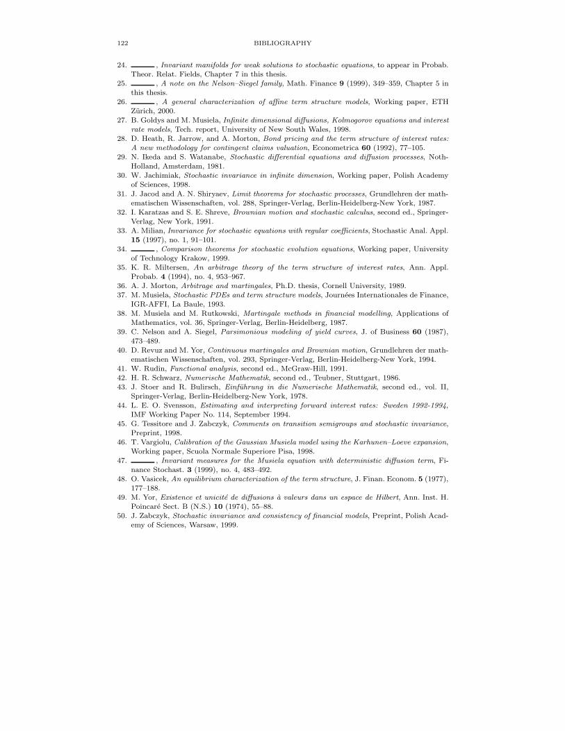
122 BIBLIOGRAPHY
24. , Invariant manifolds for weak solutions to stochastic equations, to appear in Probab.Theor. Relat. Fields, Chapter 7 in this thesis.
25. , A note on the Nelson–Siegel family, Math. Finance 9 (1999), 349–359, Chapter 5 inthis thesis.
26. , A general characterization of affine term structure models, Working paper, ETHZurich, 2000.
27. B. Goldys and M. Musiela, Infinite dimensional diffusions, Kolmogorov equations and interestrate models, Tech. report, University of New South Wales, 1998.
28. D. Heath, R. Jarrow, and A. Morton, Bond pricing and the term structure of interest rates:A new methodology for contingent claims valuation, Econometrica 60 (1992), 77–105.
29. N. Ikeda and S. Watanabe, Stochastic differential equations and diffusion processes, Noth-Holland, Amsterdam, 1981.
30. W. Jachimiak, Stochastic invariance in infinite dimension, Working paper, Polish Academyof Sciences, 1998.
31. J. Jacod and A. N. Shiryaev, Limit theorems for stochastic processes, Grundlehren der math-ematischen Wissenschaften, vol. 288, Springer-Verlag, Berlin-Heidelberg-New York, 1987.
32. I. Karatzas and S. E. Shreve, Brownian motion and stochastic calculus, second ed., Springer-Verlag, New York, 1991.
33. A. Milian, Invariance for stochastic equations with regular coefficients, Stochastic Anal. Appl.15 (1997), no. 1, 91–101.
34. , Comparison theorems for stochastic evolution equations, Working paper, Universityof Technology Krakow, 1999.
35. K. R. Miltersen, An arbitrage theory of the term structure of interest rates, Ann. Appl.Probab. 4 (1994), no. 4, 953–967.
36. A. J. Morton, Arbitrage and martingales, Ph.D. thesis, Cornell University, 1989.37. M. Musiela, Stochastic PDEs and term structure models, Journees Internationales de Finance,
IGR-AFFI, La Baule, 1993.38. M. Musiela and M. Rutkowski, Martingale methods in financial modelling, Applications of
Mathematics, vol. 36, Springer-Verlag, Berlin-Heidelberg, 1987.39. C. Nelson and A. Siegel, Parsimonious modeling of yield curves, J. of Business 60 (1987),
473–489.40. D. Revuz and M. Yor, Continuous martingales and Brownian motion, Grundlehren der math-
ematischen Wissenschaften, vol. 293, Springer-Verlag, Berlin-Heidelberg-New York, 1994.41. W. Rudin, Functional analysis, second ed., McGraw-Hill, 1991.42. H. R. Schwarz, Numerische Mathematik, second ed., Teubner, Stuttgart, 1986.43. J. Stoer and R. Bulirsch, Einfuhrung in die Numerische Mathematik, second ed., vol. II,
Springer-Verlag, Berlin-Heidelberg-New York, 1978.44. L. E. O. Svensson, Estimating and interpreting forward interest rates: Sweden 1992-1994,
IMF Working Paper No. 114, September 1994.45. G. Tessitore and J. Zabczyk, Comments on transition semigroups and stochastic invariance,
Preprint, 1998.46. T. Vargiolu, Calibration of the Gaussian Musiela model using the Karhunen–Loeve expansion,
Working paper, Scuola Normale Superiore Pisa, 1998.47. , Invariant measures for the Musiela equation with deterministic diffusion term, Fi-
nance Stochast. 3 (1999), no. 4, 483–492.48. O. Vasicek, An equilibrium characterization of the term structure, J. Finan. Econom. 5 (1977),
177–188.49. M. Yor, Existence et unicite de diffusions a valeurs dans un espace de Hilbert, Ann. Inst. H.
Poincare Sect. B (N.S.) 10 (1974), 55–88.50. J. Zabczyk, Stochastic invariance and consistency of financial models, Preprint, Polish Acad-
emy of Sciences, Warsaw, 1999.