advances in geophysics (volume49)
DESCRIPTION
Advances inGEOPHYSICSVOLUME 49Edited byRENATA DMOWSKAHarvard UniversityCambridge, MAUSATRANSCRIPT


Advances in
GEOPHYSICS
VOLUME 49

This page intentionally left blank

Advances in
GEOPHYSICSVOLUME 49
Edited by
RENATA DMOWSKAHarvard University
Cambridge, MAUSA
Amsterdam • Boston • Heidelberg • London • New York • OxfordParis • San Diego • San Francisco • Singapore • Sydney • Tokyo
Academic Press is an imprint of Elsevier

Academic Press is an imprint of Elsevier84 Theobald’s Road, London WC1X 8RR, UKRadarweg 29, PO Box 211, 1000 AE Amsterdam, The NetherlandsLinacre House, Jordan Hill, Oxford OX2 8DP, UK30 Corporate Drive, Suite 400, Burlington, MA 01803, USA525 B Street, Suite 1900, San Diego, CA 92101-4495, USA
First edition 2008
Copyright © 2008 Elsevier Inc. All rights reserved
No part of this publication may be reproduced, stored in a retrieval system or transmitted in any form or byany means electronic, mechanical, photocopying, recording or otherwise without the prior written permissionof the publisher
Permissions may be sought directly from Elsevier’s Science & Technology Rights Department in Oxford,UK: phone (+44) (0) 1865 843830; fax (+44) (0) 1865 853333; email: [email protected]. Alter-natively you can submit your request online by visiting the Elsevier web site at http://elsevier.com/locate/permissions, and selecting: Obtaining permission to use Elsevier material
NoticeNo responsibility is assumed by the publisher for any injury and/or damage to persons or property as amatter of products liability, negligence or otherwise, or from any use or operation of any methods, products,instructions or ideas contained in the material herein. Because of rapid advances in the medical sciences, inparticular, independent verification of diagnoses and drug dosages should be made
ISBN: 978-0-12-374231-5
ISSN: 0065-2687
For information on all Academic Press publicationsvisit our website at books.elsevier.com
Printed and bound in USA
08 09 10 11 12 10 9 8 7 6 5 4 3 2 1

CONTENTS
CONTENTS . . . . . . . . . . . . . . . . . . . . . . . . . . . . . . . . vCONTRIBUTORS . . . . . . . . . . . . . . . . . . . . . . . . . . . . . . ix
Chapter 1
The Generation of T Waves by Earthquakes
EMILE A. OKAL
1. Introduction . . . . . . . . . . . . . . . . . . . . . . . . . . . . . . . . 22. Geometrical Optics: Understanding T Waves in a Simple Context . . 4
Early Observations . . . . . . . . . . . . . . . . . . . . . . . . . 4T Phases as Seismo-Acoustic Conversions . . . . . . . . . . . . 7The Downslope Conversion Model . . . . . . . . . . . . . . . . 9The 1994 Bolivian T Phases . . . . . . . . . . . . . . . . . . . . 11Preferential Conversion Sites; On the Road to Scattering . . . . 13The Paradox of the Abyssal T Phase . . . . . . . . . . . . . . . . 14
3. T Waves in the Mode Formalism . . . . . . . . . . . . . . . . . . . . . 194. Using T Phases to Detect and Locate Seismic Sources . . . . . . . . . 275. Using T Waves to Explore the Seismic Source . . . . . . . . . . . . . 32
Background: Source Finiteness for T Waves . . . . . . . . . . . 34Amplitude Measurements . . . . . . . . . . . . . . . . . . . . . . 34Duration: Another Measure of Source Size . . . . . . . . . . . . 36T -Phase Energy Flux: The Parameter j . . . . . . . . . . . . . . 37The Amplitude-Duration Criterion D . . . . . . . . . . . . . . . 42The Case of the 2004 Sumatra Earthquake . . . . . . . . . . . . 51
6. Conclusion . . . . . . . . . . . . . . . . . . . . . . . . . . . . . . . . . 57Acknowledgements . . . . . . . . . . . . . . . . . . . . . . . . . . . . 58References . . . . . . . . . . . . . . . . . . . . . . . . . . . . . . . . . 58
Chapter 2
The Stress Accumulation Model: Accelerating Moment Release andSeismic Hazard
A. MIGNAN
Preface . . . . . . . . . . . . . . . . . . . . . . . . . . . . . . . . . . . 67
v

vi CONTENTS
General Introduction . . . . . . . . . . . . . . . . . . . . . . . . . . . 681. Stress Transfer Theory . . . . . . . . . . . . . . . . . . . . . . . . . . 69
1.1. Principles of Static Stress Transfer . . . . . . . . . . . . . . . . . 701.2. Seismicity Rate Changes . . . . . . . . . . . . . . . . . . . . . . 791.3. Triggering of Aftershocks by Mainshocks . . . . . . . . . . . . . 831.4. Triggering of “Preshocks” by Loading at Depth: The Stress Ac-
cumulation Model . . . . . . . . . . . . . . . . . . . . . . . . . . 852. Spatial Distribution of Accelerating Moment Release . . . . . . . . . 93
2.1. Introduction . . . . . . . . . . . . . . . . . . . . . . . . . . . . . 932.2. Methods . . . . . . . . . . . . . . . . . . . . . . . . . . . . . . . 972.3. Data . . . . . . . . . . . . . . . . . . . . . . . . . . . . . . . . . 1012.4. Results and Discussion . . . . . . . . . . . . . . . . . . . . . . . 1032.5. Appendix . . . . . . . . . . . . . . . . . . . . . . . . . . . . . . 1132.6. Supplemental Information . . . . . . . . . . . . . . . . . . . . . 115
3. Temporal Distribution of Accelerating Moment Release . . . . . . . . 1183.1. Origin of Accelerating Moment Release from Critical Processes 1193.2. Origin of Accelerating Moment Release from Stress Loading . . 126
4. Earthquake Forecasts Using Accelerating Moment Release . . . . . . 1414.1. Existing Forecasting Methods . . . . . . . . . . . . . . . . . . . 1424.2. Accelerating Moment Release and the Sumatra–Java Arc Seismic
Hazard . . . . . . . . . . . . . . . . . . . . . . . . . . . . . . . . 1534.3. Stability and Reliability of Accelerating Moment Release . . . . 1744.4. Predictability of Earthquakes Using Accelerating Moment Release 183General Conclusions . . . . . . . . . . . . . . . . . . . . . . . . . . . 190Acknowledgments . . . . . . . . . . . . . . . . . . . . . . . . . . . . . 191References . . . . . . . . . . . . . . . . . . . . . . . . . . . . . . . . . 191
Chapter 3
Seismic Ray Tracing and Wavefront Tracking in LaterallyHeterogeneous Media
N. RAWLINSON, J. HAUSER AND M. SAMBRIDGE
1. Introduction . . . . . . . . . . . . . . . . . . . . . . . . . . . . . . . . 2031.1. Motivation . . . . . . . . . . . . . . . . . . . . . . . . . . . . . . 2031.2. The Eikonal Equation . . . . . . . . . . . . . . . . . . . . . . . . 2051.3. The Kinematic Ray Tracing Equations . . . . . . . . . . . . . . 2061.4. Common Model Parameterisations . . . . . . . . . . . . . . . . . 209
2. Ray Tracing Schemes . . . . . . . . . . . . . . . . . . . . . . . . . . . 2142.1. Shooting Methods . . . . . . . . . . . . . . . . . . . . . . . . . . 2142.2. Bending Methods . . . . . . . . . . . . . . . . . . . . . . . . . . 227

CONTENTS vii
3. Grid Based Schemes . . . . . . . . . . . . . . . . . . . . . . . . . . . 2333.1. Eikonal Solvers . . . . . . . . . . . . . . . . . . . . . . . . . . . 2343.2. Shortest Path Ray Tracing . . . . . . . . . . . . . . . . . . . . . 246
4. Multi-Arrival Wavefront Tracking . . . . . . . . . . . . . . . . . . . . 2514.1. Ray Based Schemes . . . . . . . . . . . . . . . . . . . . . . . . . 2524.2. Grid Based Schemes . . . . . . . . . . . . . . . . . . . . . . . . 258
5. Concluding Remarks . . . . . . . . . . . . . . . . . . . . . . . . . . . 264Acknowledgements . . . . . . . . . . . . . . . . . . . . . . . . . . . . 267References . . . . . . . . . . . . . . . . . . . . . . . . . . . . . . . . . 267

This page intentionally left blank

CONTRIBUTORS
Numbers in parentheses indicate the pages on which the authors’ contributionsbegin
HAUSER, J. (203) Research School of Earth Sciences, Australian National Uni-versity, Canberra ACT 0200, Australia
MIGNAN, A. (67) Science & Technology Research, Risk Management Solutions,Peninsular House, 30 Monument Street, London EC3R 8NB, UK and Labo-ratoire Tectonique, Institut de Physique du Globe de Paris, 4, place Jussieu,75252 Paris Cedex 05, France
OKAL, E.A. (1) Department of Geological Sciences, Northwestern University,Evanston, IL 60201, USA
RAWLINSON, N. (203) Research School of Earth Sciences, Australian NationalUniversity, Canberra ACT 0200, Australia
SAMBRIDGE, M. (203) Research School of Earth Sciences, Australian NationalUniversity, Canberra ACT 0200, Australia
ix

This page intentionally left blank

ADVANCES IN GEOPHYSICS, VOL. 49, CHAPTER 1
THE GENERATION OF T WAVES BYEARTHQUAKES
EMILE A. OKAL
Department of Earth and Planetary Sciences, Northwestern University, Evanston, IL 60201, USA
ABSTRACT
T waves propagate in the so-called SOFAR channel of minimum sound veloc-
ity acting as a waveguide for acoustic energy in the world’s oceans. They can
be excited by sources in the solid Earth such as earthquakes through conversion
of seismic energy into acoustic waves at the solid–liquid interfaces. We present
a historical perspective of the investigations of such conversions. In the context
of geometrical optics, a sloping interface provides a mechanism for the penetra-
tion of the SOFAR channel after a series of reflections in the liquid wedge. This
process, known as “downslope conversion”, successfully explained many character-
istics of earthquake-generated T waves, but has severe limitations, notably regarding
“abyssal” T phases, generated under flat oceanic basins. We review theoretical de-
velopments based on mode theory which describe coupling between elastic and
acoustic modes under scattering by structural heterogeneities located at the ocean
bottom, and which are becoming increasingly successful at modeling the wave-
shapes of abyssal T phases.
As a particular form of seismic wave emanating from an earthquake, T waves can
provide insight into seismic sources in the oceanic environment. We review the ap-
plication of T waves to the detection of small earthquakes in marine basins, discuss
the retrieval of seismic source properties from T -phase waveforms, and show that
several algorithms combining measurements of their amplitude and duration can
yield information on source rupture, and more specifically detect the presence of
source slowness. In particular, anomalously slow earthquakes such as the so-called
“tsunami earthquakes” are poor T -wave generators, and more generally, T -phase
amplitudes and tsunami generation are not found to correlate.
In the context of the Comprehensive Nuclear-Test Ban Treaty, hydroacoustics has
been recognized as a monitoring technology, and the deployment of state-of-the-art
receivers at eleven sites will significantly improve long-range detection capabilities
and open up new opportunities for the investigation of acoustic sources, including
earthquakes, in the oceanic environment.
© 2008 Elsevier Inc. All rights reservedISSN: 0065-2687
DOI: 10.1016/S0065-2687(07)49001-X
1

2 OKAL
1. INTRODUCTION
This paper examines the generation, by earthquake sources, of the so-called T
waves guided in the water body of the world’s oceans through a channel of min-imum sound velocity generally centered around 1200 meters depth. It discussesthe mechanisms of conversion of elastic energy in the solid Earth into acousticenergy in the water, describes the potential for improving our knowledge of theseismicity of remote ocean provinces using T waves, and shows that recent de-velopments in the quantification of teleseismic T phases can help shed new lighton the high-frequency properties of earthquake source spectra.
The variation of sound velocity with depth in the ocean was originally inves-tigated in order to convert shipboard acoustic measurements into accurate depthsoundings (e.g., Langevin, 1924; Kuwahara, 1939). In simple terms, the velocityof acoustic waves in water is controlled by the thermodynamic variables de-scribing its state, namely composition, pressure and temperature. Under ambientoceanic conditions, the sound velocity increases with pressure, at a rate of about1.8 × 10−6 m s−1 Pa−1, with temperature at a rate of 2.1 m s−1 K−1, and withsalinity at a rate of 1.3 m s−1 per part per 1000 (Sverdrup et al., 1942). In theoceanic column, the pressure is hydrostatic, increasing linearly with depth, whichtranslates into a positive velocity gradient of 0.018 s−1, or 1.8 m/s per 100 m ofoceanic column. The effect of temperature is far more complex, since the thermalgradient in the world’s oceans is highly variable, both spatially and seasonally(Teague et al., 1990; Levitus et al., 1994). In most areas, the temperature dropssignificantly through the thermocline layer, and in particular in the first 150 m,and then much more slowly at greater depths. Salinity can have a highly variablebehavior in the thermocline, and stabilizes around 35 parts per thousand in thedeeper ocean. As a whole, the effect of temperature on sound velocity prevailsin the thermocline and that of pressure in the deep ocean, creating a minimum insound velocity at around 1200 m, where the resulting low-velocity channel cantrap acoustic energy with wavelengths shorter than its width, in practice with fre-quencies greater than 2.5 Hz. The existence of this waveguide was recognizedand its structure investigated early on (Swainson, 1936), but its full potential forefficient long-range propagation was realized and thoroughly studied only dur-ing World War II, as summarized upon post-war declassification by Ewing et al.(1946), who coined the acronym SOFAR (for SOund Fixing And Ranging) forthe technique and, by extension, for the low-velocity channel itself.
Irrespective of the presence of the SOFAR channel, it had long been recog-nized, apparently ever since Leonardo da Vinci (Urick, 1975), that the propagationof sound in water is particularly efficient, especially as compared to propaga-tion in the atmosphere. Modern experimental research (Urick, 1963; Thorp, 1965;Urick, 1966) has indeed documented the virtual absence of anelastic attenuationin seawater in the 1–100 Hz frequency range, which serves to further enhance the

THE GENERATION OF T WAVES BY EARTHQUAKES 3
efficiency of the SOFAR channel, and sets the finite size of the ocean basins asthe only physical limit to the range of SOFAR propagation.
Despite the variability of the detailed characteristics of the sound velocityprofile (depth of SOFAR axis, minimum velocity, reciprocal depth, etc.), the ex-istence of the channel is a quasi-universal feature, the only possible exceptionsinvolving the cold waters of the extreme Southern Ocean from which the thermo-cline is absent. Its ability to propagate energy from exceptionally small sourcesover remarkably large distances has found applications world-wide in fields asvaried as the tracking of submarines, the discovery and monitoring of distant vol-canoes (Dietz and Sheehy, 1954; Norris and Johnson, 1969; Talandier and Okal,1982, 1996; Fox et al., 1995), the detection of explosions in the oceanic envi-ronment, notably in the context of the Comprehensive Nuclear-Test Ban Treaty(CTBT) (Milne, 1959; Adams, 1979; Okal, 2001a; Wallace and Koper, 2002;Reymond et al., 2003; Talandier and Okal, 2004a), the detection of iceberg col-lisions in the Southern Ocean (Talandier et al. 2002; 2006), the study of thevocalization patterns of large cetaceans (Reysenbach de Haan, 1966; Stafford etal., 1998), and the monitoring of global warming (Munk et al., 1994).
While SOFAR propagation is limited to the oceanic column, acoustic en-ergy in the water can be transformed to and from elastic energy at the solid–liquid interfaces marking the boundaries of an oceanic basin, and this mecha-nism, whose degree of complexity can vary widely, allows both the excitationof acoustic energy by sources in the solid Earth, such as earthquakes and un-derground explosions, and its recording by land-based seismic stations locatednear the shore or even, under exceptional circumstances, hundreds of kilometersaway from the coastlines (Båth and Shahidi, 1971; Cansi and Béthoux, 1985;Pasyanos and Romanowicz, 1997). Indeed, when the seismic wave resulting fromthe receiver-side conversion is of sufficient amplitude, it can be felt by the pop-ulation close to the shore, even though the source of the acoustic energy maybe many thousands of kilometers away. Examples include the underwater nu-clear explosion WIGWAM on 14 May 1955, felt in Hawaii (J.P. Eaton, pers.comm., 1979) and even in Torishima, 8750 km from the source (Wadati, 1960);the Fairweather, Alaska earthquake on 10 July 1958 felt in Hawaii (J.P. Eaton,pers. comm., Eaton, 1979); the Tonga earthquake on 22 June 1977 felt in Tahiti(Talandier and Okal, 1979); the South Island, New Zealand earthquake of 21 Au-gust 2003 felt in Sydney, Australia (Leonard, 2004); and as discussed below, thegreat 2004 Sumatra earthquake felt in the Maldives (A.C. Yalçıner, pers. comm.,2005). In addition, T waves from certain Venezuelan earthquakes are routinelyfelt in Puerto Rico at a somewhat shorter distance (not exceeding 900 km) (C.G.von Hillebrandt-Andrade, pers. comm., 1998). Note that coupling is also possi-ble, at least in principle, with the atmospheric column; however, the mechanicsof the conversion of air waves into acoustic phases are poorly understood, due tothe scant number of adequate sources, consisting exclusively of large atmosphericnuclear tests in the early 1960s (Talandier and Okal, 2001, 2004b).

4 OKAL
As discussed more in detail below, earthquake-generated hydroacoustic wave-trains were first identified as a far-field phase on seismograms (if not correctlyinterpreted) in 1935 by scientists at Harvard Observatory upon recording ofCaribbean earthquakes (Collins, 1936), and given the name T group (for “Ter-tiary” arrival, following P , primary and S, secondary) during informal discussionsof these phases by the Harvard staff (Leet et al., 1951). To our knowledge, thisname first appeared in print in Linehan (1940).
When T waves were later correctly identified as water-borne waves guided bythe SOFAR channel, a major problem arose, as the excitation of T waves trappedin the channel from earthquake sources located in the solid Earth, and thus bynecessity outside the waveguide, is theoretically impossible in the framework ofgeometrical optics applied to a simple flat-layered Earth model. Indeed, all ac-ceptable sound velocity profiles predict that only rays inclined less than ∼12◦on the horizontal can be trapped in the channel, while the sharp contrast in seis-mic and acoustic velocities in the source region precludes the penetration of theoceanic column at all but the steepest incidences.
In this framework, the present paper offers a largely chronological review offive decades of observational developments and theoretical efforts, seeking to re-solve the apparent paradox of the ubiquitous observation of efficient excitationand propagation of far-field T phases from earthquake sources, through a seriesof modifications to the simple flat-layered model based on geometrical optics. Itfurther discusses various efforts at quantifying the energy present in T phases, in-cluding recent developments that use their characteristics to explore the dynamicsof the seismic source.
The discussion of the excitation of T waves by acoustic sources in the watercolumn, such as man-made underwater explosions, magmatic episodes of volcan-ism delivering magma to the ocean floor, or the generation of cryosignals duringcollision between large icebergs, is intentionally left out of the present review.
2. GEOMETRICAL OPTICS: UNDERSTANDING T WAVES IN A SIMPLE
CONTEXT
Early Observations
To our knowledge, the first published report of a teleseismic T wavetrain goesback to Jaggar (1930), who describes high-frequency oscillations recorded atHawaii Volcano Observatory (HVO) in the coda of a major earthquake whichtook place on 24 October 1927 on the Fairweather Fault of the Alaska pan-handle (Fig. 1). However, Jaggar interprets the record as local volcanic tremor“possibly touched off by the big earthquake waves”. A modern examination ofthe spindle-shaped waveform, frequency content and timing of the phase (quotedas 06:20 a.m. HST or 16:50 GMT) definitely identifies it as the T wave of the

TH
EG
EN
ER
AT
ION
OF
TW
AV
ES
BY
EA
RT
HQ
UA
KE
S5
FIG. 1. Left: Seismic recording of the Alaskan earthquake of 24 October 1927 at Hawaii Volcano Observatory, after Jaggar (1930). This is believed to be thefirst published record of a teleseismic T phase. The top trace is the S–N component, the lower one, the E–W component; time increases from right to left andfrom top to bottom. The window is approximately 200 seconds long. Right: Maps sketching the transpacific path of the T phase from source (star) to receiver,and the location of the receiver station inside the “Big” Island of Hawaii. Adapted from Jaggar (1930).

6 OKAL
Alaskan earthquake. Note that Jaggar mentions that the phase was “feebly felt” inHawaii, as would later be the larger 1958 earthquake, in a very similar geometry.
Several years later, Collins (1936) noted in the Seismological Bulletin of Har-vard Observatory that the record of the Caribbean earthquake of 15 September1935 featured a third arrival, following P and S, detected exclusively on short-period channels. This constitutes the first correct interpretation of a T wave as theindependent phase of a distant earthquake. Our relocation of that earthquake basedon travel-times published in the International Seismological Summary (ISS) andthe algorithm of Wysession et al. (1991) converges on 19.03◦N, 64.85◦W and adepth of 64 km, although the Monte Carlo ellipsoid (run with a standard devia-tion σG = 4 s for the Gaussian noise injected into the dataset) does intersect theEarth’s surface. It is nevertheless probable that the earthquake occurred at depth inthe Puerto Rico trench as suggested by reports of weak surface waves, and in gen-eral agreement with the local patterns of seismicity (Fischer and McCann, 1984).Based on this hypocenter, we have verified that the time given by Collins (1936)as the emergence of the “third group” (04:28:20 GMT) supports its interpretationas a T phase converted to a seismic wave approximately 3◦South of the receiver.Subsequent detections of T phases are also reported in the Harvard Bulletin forseveral Caribbean earthquakes, notably on 18 September and 10 November 1935(the latter relocating about 40 km West of Montserrat), and 12 December 1936.
Such observations were analyzed in greater detail by Linehan (1940) who onlyoffered speculation as to their nature; in particular, his published illustration ofthe waveshapes (Fig. 2) appears to be no more than a hand-drawn rendition oftheir timing. More insightful is Ravet’s (1940) contemporaneous but obviouslyindependent report on very short period signals recorded in Tahiti in the wake ofdistant major earthquakes: the author correctly establishes their association withthe epicenter, their generation by the seismic source and their propagation alongthe surface of the Earth as opposed to through its body. He does estimate a groupvelocity of 1.5 km/s, but stops short of identifying the latter as the velocity ofsound in water, which had been known since the work of Beudant in the Mediter-ranean Sea in the 1810s and the landmark experiments of Colladon and Sturm(1827) in Lake Geneva.
Indeed, the correct interpretation of T waves as water-borne phases of theseismic source would come only in the wake of the considerable progress in hy-droacoustics achieved during World War II, as summarized in a special volume ofthe Geological Society of America, in which Ewing and Worzel (1948) publishedthe basics of long range propagation in the SOFAR channel, and Pekeris (1948)developed elementary models of the structure of T waves, based on modal theory.These works were complemented by the experimental results of Worzel and Ew-ing (1948). Simultaneously and independently, Brekhovskikh (1949) published amodel for the reverberation of sound in the channel, based on experimental resultsby Rozenberg (1949).

THE GENERATION OF T WAVES BY EARTHQUAKES 7
FIG. 2. Reproduction of Linehan’s (1940) Fig. 4 (complete with original caption), showing asketch of T phases from Caribbean earthquakes recorded at Harvard Observatory in the late 1930s.Note that even though the records have been arranged by distance (based on S − P times), theT phases (emphasis added) arrive at irregular times, illustrating the variability of the source-side con-version process; this certainly hindered any simple interpretation of the phase by the author. Thediagram was probably hand-drawn, and does not reproduce the waveshape of the T phases; note10-minute gap in the time scale between the left and right parts of the figure. Adapted from Linehan(1940).
T Phases as Seismo-Acoustic Conversions
In a number of seminal papers published in the early 1950s, W. Maurice Ew-ing and his collaborators established the bases of the generation of T phasesby earthquakes, as resulting from the conversion of seismic energy to acousticwaves at a source-side solid Earth–liquid ocean interface, followed by the reverseacoustic-to-seismic conversion at the receiver side (Tolstoy and Ewing, 1950).A fundamental aspect of this model is that the existence of sloping interfaces al-lows the trapping of acoustic energy inside the low-velocity waveguide and henceits efficient propagation to teleseismic distances. In particular, using Caribbean,North and South American earthquakes recorded at Bermuda, Shurbet and Ewing(1957) conclusively modeled their T waves as resulting from conversion of P orLg phases at an isobath which they selected as 1800 m.
Such models were initially not without detractors, and in particular, Leet (1951)and Leet et al. (1951) argued, using occasionally vehemently forceful rhetoric,

8 OKAL
FIG. 3. Principle of the generation of a T phase from an underground source by downslope con-version. The source-side seismic ray (labeled P ) is converted at the ocean bottom into a steep acousticray which is reflected back and forth between the sea surface and the sea floor. In the presence of aninterface sloping at an angle α, the incidence of the ray is decreased by 2α at each bottom reflection,and penetration becomes possible after a handful of reverberations. Adapted (cropped and new labels)from Johnson et al. (1963).
that T phases rather represent energy channeled through ocean-bottom sedimen-tary layers, an idea already expressed by Coulomb and Molard (1949). Later work(e.g., Okal and Talandier, 1981) has indeed documented the possibility of long-range propagation of such waves, but at generally lower frequencies, and withconsiderable group dispersion (from 0.5 to 2 km/s), not observed in T phases.In their response to Leet’s criticism, Ewing et al. (1952) correctly pointed out theneed for a careful decomposition of the path into its seismic and acoustic portions.When the former become significant, they invalidate any estimate of the velocityof the T phase simply averaged over the entire distance from the source to thereceiver.
Despite these early controversies, the work of Ewing and collaborators haswithstood the trial of time, in particular concerning the timing of earthquake-generated T waves, which they successfully modeled by summing the contribu-tions of the various seismic and acoustic segments (Shurbet, 1955). In their secondpaper on T waves in the Lesser Antilles, Coulomb and Molard (1952) reachedsimilar conclusions, but emphasized the importance of S → T conversions inspecific geometries. At the same time, Wadati and Inouye (1953) underscoredthe role of steep slopes for efficient conversions, and again of source-side S → T
conversions notably for moderately deep (70 km) Japanese earthquakes.In retrospect, it is remarkable that Ewing’s group successfully developed their
model in the Caribbean-to-New England geometry, which requires complex andlong seismic conversions at both ends of the paths. In particular, Fig. 2 (fromLinehan (1940)) clearly illustrates the lack of correlation for such paths betweenthe precise timing of T and distance expressed by S − P intervals. By contrast,Ravet (1940) was helped in his interpretation by the generally greater epicentraldistances and minimal converted paths at the receiver side in Tahiti.

THE GENERATION OF T WAVES BY EARTHQUAKES 9
The Downslope Conversion Model
Considerable insight was gained throughout the 1960s from the operation, prin-cipally by the University of Hawaii, of a wide-aperture network of hydrophonestations throughout the Pacific Basin (Wake, Enewetak, Midway, Oahu, PointSur). In this framework, Johnson et al. (1963) soon developed the concept of“downslope conversion” (Fig. 3), originally proposed by Officer (1958). In thepresence of a beach sloping at an angle α, reverberations of acoustic rays betweenthe seafloor and the ocean surface are deflected by 2α at each successive cycle,which eventually allows trapping of the energy inside the SOFAR channel at anangle inclined less than 12◦ on the horizontal, even though all acoustic rays at theoriginal conversion point would remain much steeper.
The downslope conversion model, based entirely on geometrical optics, provedhighly successful at explaining many attributes of the observed T wavetrains. Inparticular, Johnson et al. (1963) modeled lateral changes in the strength and wave-shapes of T phases observed at Kaneohe Bay, Oahu from a series of hypocentersin the Andreanof Islands, based on variations in the number of reflections neces-sary for trapping through downslope conversion. Milne (1959) had used a similarconcept to constrain the source of two nuclear tests to the interior of Enewetaklagoon, based on the spectral properties of their teleseismic T waves, which heinterpreted as resulting from downslope conversion.
More recently, Talandier and Okal (1998) contrasted T waves received at theFrench Polynesian Seismic Network (Reseau Sismique Polynésien or RSP), fromvarious types of earthquakes occurring on the Southern part of the Island ofHawaii (Fig. 4). For shallow earthquakes originating near the shoreline, character-ized in that area by steep (up to 50◦) subaerial and underwater cliffs (the “palis”),the T wavetrains are impulsive, of high amplitude, and feature a fast group time,as a result of a simple conversion process, requiring no more than one reflection topenetrate the SOFAR channel (Fig. 4A). In contrast, for deeper events occurringunder the more gentle slopes (typically 15◦) of the nearby Loihi volcanic edifice,the T waves are emergent, spindle-shaped, much lower in amplitude, and featurepositive delays, as the conversion process requires as many as five back-and-forthreverberations, and is delocalized along the liquid–solid interface (Fig. 4B). Inthe former geometry, Talandier and Okal (1998) showed that the waveshape ofthe teleseismic T phase is a simple transposition of the ground motion at the con-version point, as recorded for example by a seismic station in the near field. It isdominated by the P → T and S → T conversions, the latter featuring a charac-teristic time delay and a lower frequency content.
Such differences in the efficiency of the conversion process can be transposedto the case of the acoustic-to-seismic conversion at the receiver side, where theycan govern the siting of the so-called T -phase seismic stations designed to pro-vide high-quality seismic recording of hydroacoustic phases, as mandated underthe CTBT (Okal, 2001a). In particular, Okal and Talandier (1998) provided guide-lines to define station corrections, in order to account for the receiver-side seismic

10 OKAL

THE GENERATION OF T WAVES BY EARTHQUAKES 11
FIG. 4A. Comparison of the T waves recorded at Pomariorio (PMO) from two earthquakes on andnear the Big Island of Hawaii. Right: The maps sketch the general geometry of the focal areas andthe path to Polynesia. The 1993 earthquake is located under the steep Poliokeawe “pali” [cliff], whilethe 1996 event took place deeper and under gentler slopes at Loihi seamount. Left: Seismogram ofthe T phase of the 1993 Pali event at PMO (Top) and modeling of the conversion (Bottom). Note theimpulsive character of the phase, and the clear separation of the P → T and S → T wave packets.The modeling shows an efficient conversion, requiring only one reverberation, at the steep slope im-mediately off the shoreline (circles). In this geometry, the T phase is predicted to arrive early relativeto acoustic propagation along the whole path, as observed on the record. Adapted (combined; mapadded) from Talandier and Okal (1998).
path, and showed that S → T conversions could become prominent under cer-tain combinations of structure and distance between shore and receiver leading toshadowing for the converted P wave.
The 1994 Bolivian T Phases
The generation of T phases by intermediate-depth (70 � h � 300 km) ordeep (h � 300 km) earthquakes was mentioned in the very earliest studiesby Linehan (1940), Ewing et al. (1952) and Shurbet (1955), the latter noticingthat a deep focus actually favors T -phase generation for large South Americanearthquakes recorded at Bermuda. We now attribute such observations to the ab-sence of a source-side asthenospheric path otherwise generally responsible for thestrong anelastic attenuation, in teleseismic or even regional S waves, of the high-frequency components exclusively capable of penetrating the SOFAR channel.
This remark led to an unexpected development upon the recording (Fig. 5) ofspectacular T waves across the entire Pacific Basin following the great 1994 deepBolivian earthquake (Kirby et al., 1995), an observation itself intriguing given theconsiderable distance of its 631-km deep source from the oceanic water mass.†
Okal and Talandier (1997, 1998) further documented that the timing of the Bo-livian T waves at receivers across the Pacific required source-side conversion ofregional S waves, principally at the Arica Bight. This observation was impor-tant from a structural point of view, since the delivery by an S wave, 920 kmaway from the source, of the high frequencies needed to penetrate the SOFAR(by necessity f � 2.5 Hz; f ≈ 5 Hz as observed) requires propagation throughmaterial with exceptionally low anelastic attenuation. In turn, this implies thecontinuity of the cold slab throughout the upper mantle, despite the presence of agap in seismic activity between 300 and 600 km depth in the local Benioff zone,which had led early investigators to propose a broken or detached slab (Isacks and
† Indeed, there exists some scant anecdotal evidence that the Bolivian T phase may have been felton the Southern shore of the “Big” Island of Hawaii (G.J. Fryer, pers. comm., 2000).

12 OKAL
FIG. 4B. Same as Fig. 4A for the 1996 Loihi earthquake. Top: T phase record at PMO. Note theemergent phase, with no clear separation of its various components. Also, the phase is significantly laterelative to a pure acoustic path from epicenter to receiver. Bottom: Modeling of the P → T and S → T
conversions in the presence of a gently sloping beach. In (a) and (b), we show rays departing the focusat 1 and 10◦ incidence angles. Each requires several reverberations to penetrate the SOFAR channel,and when combined in (c), this results in a wavetrain of longer duration. Frame (d) shows similarcharacteristics for the S → T conversion. Adapted (combined) from Talandier and Okal (1998).
Molnar, 1971). An S → T conversion from a deep earthquake then constitutes aproxy for a thermally, and hence mechanically, continuous, low-attenuating slabin the source region, and Okal (2001b) later applied the concept to the so-called“detached” or “outboard” earthquakes, proving in most instances (e.g., Sakhalin,Bonin Islands) that these occurred in warped, rather than detached, segments ofthe slab. In this framework, T phases can provide an unexpected insight into thedeep structural properties of the Earth’s mantle.

THE GENERATION OF T WAVES BY EARTHQUAKES 13
FIG. 5. Examples of T phases generated by deep earthquakes at the bottom of subduction zones.Left: Case of the 1994 Bolivian earthquake. The top figure presents a high-pass filtered waveform atRarotonga and the corresponding spectrogram. Note the presence of a single wave packet, identifiedby Okal and Talandier (1997, 1998) as an S → T conversion at the Arica Bight. The bottom figureshows the geometry of the source side conversion. Right: Case of the so-called “detached” 1990 deepearthquake under Sakhalin, recorded at Pomariorio (French Polynesia). Note the presence of two sep-arate wave packets, corresponding to P → T and S → T conversions, respectively. The presence ofthe latter requires the continuity of a finger of cold slab, despite the location of the earthquake outboardof the conventional location of the slab. Also, in both instances, note the location of the conversionpoints at preferential sites along the coast line. Adapted (combined; new material added) from Okaland Talandier (1997) and Okal (2001b).
Preferential Conversion Sites; On the Road to Scattering
A by-product of Okal’s (2001b) investigation was the documentation of pref-erential sites of source-side conversion, such as the Arica Bight for the deepBolivian earthquake, and Cape Erimo in Southern Hokkaido, for the Sakhalinone (Fig. 5). This observation was in line with Johnson and Norris’ (1968) studyof the T waves generated by the 1965 Rat Island aftershock series, which iden-tified loci of preferential conversion for an otherwise largely uniform field ofseismic epicenters. Similarly, Walker et al. (1992) documented occasional pre-cursors to T phases, attributed to conversion at seamounts neighboring Alaskanand Aleutian epicenters. While observations such as Okal and Talandier’s (1997)are still reconcilable with geometrical optics by invoking focusing due to strong

14 OKAL
FIG. 5. Continued.
curvature of the mid-SOFAR isobath, Walker et al.’s (1992) results suggest theinfluence of scattering in the generation process.
The Paradox of the Abyssal T Phase
Furthermore, non-geometrical processes are clearly required to explain theparadox of the so-called “abyssal T phase” sketched on Fig. 6. In this instance,a small intraplate earthquake occurring in a flat abyssal plain, far away from anydocumented shallow slope, generates a strong T wave throughout the Pacific,whose group times are compatible with generation at the time and epicenter ofthe seismic source. Note in particular that this property holds not only in the farfield (RAR), but also at regional distances (PTCN; 400 km). This indicates thatthe acoustic wave can be generated in a variety of azimuths in the immediatevicinity of the epicenter, in the absence of a relief appropriate for downslope con-version, and with a minimal, or absent, source-side seismic path. This scenario isreminiscent of Johnson et al.’s (1968) observation (Fig. 7) of two components tothe T wave of an outer rise Aleutian earthquake (mb = 6.3; 29 July 1965), the rel-atively impulsive, low-frequency and high-amplitude “downslope” arrival beingexpectedly late (by ∼2 minutes), but preceded by an “abyssal” arrival featuringhigh frequencies, a low amplitude, and an emergent wavetrain, which appears tooriginate at the time and location of the seismic source.
In attempting to explain the abyssal T phase, we note that Biot (1952) had ini-tially proposed that a strong coupling could develop between “SOFAR waves” and

THE GENERATION OF T WAVES BY EARTHQUAKES 15
FIG. 5. Continued.
Stoneley waves generated at the solid–liquid interface, which could provide themechanism for the excitation of an abyssal T phase. However, he did not elabo-rate beyond the observation that the two systems may have comparable dispersioncurves in the high-frequency limit, which may be a necessary but not sufficientcondition for the actual development of coupling. This concept was revived re-cently by the observation by Butler and Lomnitz (2002) of a so-called Ti wave,which they define as featuring the propagation characteristics of T phases, while

16O
KA
L
FIG. 6. Example of abyssal T phases generated by a “true” intraplate earthquake, occurring outside any large scale bathymetric feature, (a), (b) and (c):Situation maps of the relevant source and paths. The shaded box in (a) outlines Frame (b). Note the smooth bathymetry of the epicentral area, (d) and (e):Seismograms observed at Rarotonga (RAR) and Pitcairn (PTCN), respectively, high-pass filtered at 1.5 Hz, with relevant spectrograms. Note the long duration(80 s), and emergent character of the T phase, which arrives at a group time in agreement with acoustic propagation along the whole path. The vertical arrowsindicate group times calculated from the epicenter for v = 1.483 km/s, and in the case of PTCN, the origin time, and Pn and Sn arrivals. Note that the latter isthe dominant phase.

TH
EG
EN
ER
AT
ION
OF
TW
AV
ES
BY
EA
RT
HQ
UA
KE
S17
FIG. 6. Continued.

18 OKAL
FIG. 7. Combination of abyssal and downslope generation of the T phase for the Aleutian earth-quake of 29 July 1965 recorded at Kaneohe, Oahu (after Johnson et al., 1968). Top: Map of thesource area, showing the epicentral location (star), and the proposed sites of downslope (square)and abyssal (circle) conversions. Center: Spectrogram of the T phase contrasting the late, impulsive,high-amplitude and low-frequency downslope arrival with the earlier, emergent, higher-frequency butlower-amplitude abyssal arrival. Bottom: Model of abyssal generation as proposed by Johnson et al.(1968). The T phase is generated from scattering by an irregular sea surface, in the immediate vicinityof the epicenter, and thus suffers practically no delay, as compared to the downslope-converted phasewhich first backtracks as a P wave an estimated 150 km. Adapted (combined; cropped; re-labeled)from Johnson et al. (1968).

THE GENERATION OF T WAVES BY EARTHQUAKES 19
FIG. 7. Continued.
being detected on ocean-bottom or borehole instruments, i.e., in a geometricalshadow for waves guided in the SOFAR channel. However, their model of thepropagation of Ti in a layer of relatively loose sediments on the ocean floor raisesthe question of the effect of anelastic attenuation (expected to be high in suchstructures) on the high frequencies characteristic of the phase.
This leaves a non-geometrical process, such as scattering, as the probablemechanism of generation of the abyssal T phase. Johnson et al. (1968) initiallyattributed its origin to sea surface roughness (Fig. 7), while Keenan and Merriam(1991) later suggested underside scattering by sea ice in the Arctic Ocean, an in-terpretation obviously limited to polar regions. Later, and most decisively, Foxet al. (1994) invoked broad-band scattering by a rough seafloor in the generalframework of modal propagation, which forms the basis of the presently consen-sual interpretation of the abyssal T phase.
3. T WAVES IN THE MODE FORMALISM
Modal theory envisions T waves as the superposition of a discrete, albeit inprinciple infinite, number of modes of surface waves guided by the oceanic col-umn, and in particular by the SOFAR channel. The fundamental framework ofthis approach was developed by Pekeris (1948). Given a flat-layered structurefeaturing translational symmetry along the horizontal x and y directions, the po-tential φ of the elastic wave in the water is sought at each angular frequency ω asa cylindrical wave radiating out of the polar axis r = 0:
(1)φ(r, z, t) = �(z)H(1)0 (kr) e−iωt ,

20 OKAL
where H(1)0 is the Hankel function of first kind and order 0, and � satisfies
(2)d2�(z)
dz2+[
ω2
v2(z)− k2
]�(z) = 0,
v being the local velocity of sound, which can be a priori a function of depth z.The boundary conditions, imposing zero pressure at the ocean surface, and zerodisplacement either at a rigid bottom or as z → ∞, control the existence, ateach frequency, of a finite number of eigenmodes expressing the relationship be-tween ω and the wave number k, and analogous to the fundamental and overtonesof a classical Rayleigh wave.
In his initial study, predating the era of high computational power, Pekeris(1948) first considered the oversimplified model of a single oceanic layer over aliquid half-space (Fig. 8a), and explored analytically the properties of the funda-mental and first few overtones, closely following Love’s (1911) classical analysisof the transverse shear modes of a solid layer over a solid half space. He thenextended his investigation to a model featuring two layers over a half space(Fig. 8b), more representative of the SOFAR channel, but still involving exclu-sively liquids. Pekeris was able to describe the essential dispersive properties ofthe various branches, in particular the existence of one or several group velocityminima, for various contrasts in sound velocities and layer thicknesses. Most re-markably, he also laid the groundwork for the computation of the excitation of thevarious modes by an explosive source located in the water, by following Lamb’s(1904) classical decomposition of the solution into an integral in the complexwavenumber plane. Such results were remarkably insightful given the simplifiedrepresentation of the oceanic column as a single layer over a liquid half space,and for that reason, this model, known as a “Pekeris waveguide”, has remained abenchmark reference for comparisons with modern, much more sophisticated andaccurate models of the oceanic column.
Over the next decades, and as detailed for example in Jensen et al.’s (1994)comprehensive monograph, improvements in computational techniques, as wellas the systematic three-dimensional surveying of the properties of the ocean, haveled to more sophisticated models of the structure of guided propagation in theSOFAR channel and of the excitation of acoustic modes by oceanic or land-basedsources. Obviously, these developments owed much to the parallel investigationof the theory of seismic waves in layered structures, notably for surface wavesby Haskell (1953) (and Harkrider (1964) regarding their excitation by varioussystems of forces), and for body waves as summarized by Kennett (1983). Thefollowing are the milestones most important to our understanding of the excitationand propagation of T waves by earthquake sources.
• The use of realistic velocity profilesBased on a combination of experimental and theoretical work (Tolstoy and
Clay, 1966; Pedersen, 1969), Munk (1979) provided an analytical representation

THE GENERATION OF T WAVES BY EARTHQUAKES 21
(a) Assumed model for a two-layered liquid half-space
(b) (c)
FIG. 8. Reference models used in theoretical studies of the structure and generation of acousticmodes of the oceanic column. (a): The Pekeris waveguide, consisting of a liquid layer over a liquidhalf-space; all parameters can be widely varied. (b): Pekeris’ later model of a low velocity waveguide,consisting of two layers over a substratum, all media remaining liquid; velocities in ft/s; (c): TheMunk sound speed profile described by Eq. (3). Adapted (rescaled; combined; re-labeled) from Pekeris(1948) and Jensen et al. (1994).

22 OKAL
of a reference velocity profile in the oceanic column,
(3)v(z) = v0
[1 + ε
(z − 1 + e−z
)]; z = 2
(z
zaxis− 1
)
where v0 = 1500 m/s, ε = 0.00737, and zaxis = 1300 m. This model, known asthe Munk profile and shown on Fig. 8c, features a well-developed SOFAR channelcentered around the depth zaxis. The Sturm–Liouville nature of the problem thenallows the use of efficient algorithms (e.g., Wilkinson, 1965) for the systematiccomputation of literally hundreds of overtones over a wide range of frequencies.The duality between the modal solutions and the optical ray representation canthen be investigated in the framework of the WKB approximation (e.g., Ewing etal., 1957; Tindle, 1979). In general, as the mode (overtone) number n is increasedat any given frequency, the phase velocity increases, which amounts to steepeningthe incidence of the equivalent ray.
• The use of realistic boundary conditionsThe effect of the rigidity of the ocean bottom was addressed early on by Press
and Ewing (1950), who considered the case of a single liquid layer over a solidhalf-space, in particular for an explosive source in the water column. They ob-tained fundamental results, especially regarding the influence of the finite valueof the rigidity of the bottom on the apparent dispersion of the acoustic wave.More systematic investigations of this model (Brekhovskikh and Lysanov, 1982;Jensen et al., 1994) have suggested that the reflection on the solid bottom is wellapproximated by a Pekeris model in which the sound velocity in the liquid sub-stratum would equal the shear velocity of the solid half-space. This importantremark justifies a posteriori the use of the oversimplified Pekeris model.
Figure 9, adapted from Park et al. (2001), contrasts, at a single frequency (inthis case 5 Hz), the eigenfunction of the first overtone mode (not counting the in-terface Stoneley mode), with that of a higher (“hybrid”) overtone. The former hasits energy concentrated around 1000 m depth, in the axis of the SOFAR channel;its properties are equivalent to those described by Pekeris (1948), and in particular,its phase velocity, C = 1.483 km/s, expresses propagation of the acoustic energyin the channel. But because its eigenfunction has become essentially negligibleby the time it reaches the solid substratum, such a mode cannot be excited by anysource in the solid Earth. By contrast, Mode 32 has a well-developed eigenfunc-tion both in the first 12 km of the solid Earth and in the water column; howeverits phase velocity, C = 3.438 km/s, indicates that its energy mostly reverberatesat a steep incidence (25◦) between the surface and bottom of the ocean, and doesnot propagate laterally in the SOFAR channel. In this framework, modal theorycannot explain the excitation of an abyssal T phase in a flat-layered structure anybetter than its geometrical optics dual, namely ray theory.

TH
EG
EN
ER
AT
ION
OF
TW
AV
ES
BY
EA
RT
HQ
UA
KE
S23
FIG. 9. Theoretical modal solutions reproduced from Pekeris (1948) and Park et al. (2001). (a): Pekeris’ solution, obtained for his waveguide model shownon Fig. 8b; the plot shows the depth variation of the pressure eigenfunction. (b): First overtone solution at a frequency of 5 Hz, computed by Park et al. for a2.25-km deep ocean featuring a SOFAR channel; the black line is the eigenfunction of the vertical displacement, the red one that of the horizontal displacement.Note that the mode does not penetrate appreciably the solid Earth. (c): Same as (b) for the 32nd overtone mode, plotted using a different vertical scale. Note thatenergy is present both in the liquid and solid, but the larger phase velocity expresses the inefficient lateral propagation of the energy in the liquid layer. Adapted(combined; rescaled; re-labeled) from Pekeris (1948) and Park et al. (2001).

24 OKAL
• The computation of the excitation of the modesAt any given frequency, the excitation of the various modes by any source in
the ocean column (taken as a point source explosion) or in the solid Earth (takenas an elastic dislocation) is readily computed in the formalisms of Saito (1967) orGilbert (1970). The summation of the various modes, weighted by their appropri-ate excitation, allows the synthesis of the wavetrains propagating away from thesource, just as the summation of the free oscillations of the Earth excited by anearthquake yields a synthetic seismogram featuring the familiar seismic phasesobserved at teleseismic distances (Brune, 1964).
• The application of perturbation theory in the modal frameworkThis allows the study of mode coupling induced by [weak] lateral heterogeneity
of the layered structure under consideration. Most such efforts have consideredtwo types of heterogeneity: one involves two flat basins with different waterdepths, with a smooth transition extending over several wavelengths, the othera single basin with localized irregularities of the ocean floor, of an amplitudecomparable to the acoustic wavelengths (Fig. 10a, b). Based on earlier theoreti-cal work by Shevchenko (1962), Pierce (1965) and Milder (1969), Odom (1986)investigated a number of such scenarios, and in particular, for the second case, de-rived coupling coefficients between the various modes of the water column. In layterms, this means that a corrugated structure of the type shown on Fig. 10b canprovide a mechanism to leak energy from modes with little if any amplitude inthe SOFAR channel (but strongly excited by underwater earthquake sources) intomodes representing propagation of energy trapped into the channel (but not ex-citable by underground sources). This approach provides the key to a satisfactoryexplanation of the generation of the abyssal T phase by scattering at the oceanbottom.
More recently, Park and Odom (1999) extended the concept to the case of astochastic field of heterogeneities on the seafloor, and Park et al. (2001) appliedtheir results to a number of scenarios involving different geometries and depths ofearthquakes under both a homogeneous ocean–bottom interface, and a heteroge-neous one, which could be deterministic (as in the case of the sloping interface)or stochastic (i.e., featuring random roughness). Figure 10c (adapted from Park etal. (2001) quantifies, for a flat-layered structure and at f = 5 Hz, the seismic am-plitude excited into the various overtone branches, and illustrates that only thosemodes with overtone numbers n = 18–55 are significantly excited. Figure 10dsimilarly shows the kernels for conversion of the elastic field in (c) by variousscatterers located at the ocean bottom. Once multiplied by a scattering functionexpressing the density of heterogeneity in models such as (a) or (b), the kernelsyield the cross-over amplitudes converted into the various modes. Note that thehorizontally propagating water modes (n = 1–10) are now excited with a finiteamplitude; this expresses the key result of the model, namely that it can indeedpredict the excitation of an abyssal T phase.

THE GENERATION OF T WAVES BY EARTHQUAKES 25
(a)
(b)
FIG. 10. (a) Example of lateral perturbation of a flat-layered ocean model: Two basins of depths h1and h2 are connected by a slope. (b): Model of a corrugated segment of ocean floor in an otherwise lat-erally homogeneous flat-layered structure. (c): Initial excitation, at f = 5 Hz, of the various overtonemodes of a flat-layered structure by a double-couple source located at 9 km depth (the ocean layer,2.25 km deep, is shown in darker tone). Note that only overtones of order 18–55 are substantiallyexcited. In particular the lower overtones corresponding to propagation in the water column are not.(d): Mode excitation by sea-bottom scattering. Note that the energy of the higher modes in (c) hasbeen converted into the lower overtones (of order less than 10), propagating in the SOFAR channel.See text for details. Adapted (combined; re-labeled) from Odom (1986) and Park et al. (2001).
Park et al. (2001) further documented that relatively deep earthquakes (h =80 km) can excite T waves through scattering by a rough ocean bottom, andalso proposed that strike–slip earthquakes seem especially efficient at generatingT phases, as observed by Dziak (2001), and further discussed below.
Finally, Odom and Soukup (2004) examined the amplification of the scatteringprocess in the presence of an intermediate layer of low-rigidity sediments, whichcan be regarded as the mode dual of the well-known amplification of strong mo-tion by sedimentary structures routinely observed in classical seismology (e.g.,Gutenberg, 1957; Bard et al., 1988).
Following a different strategy, Schmidt et al. (2004) model the scattering ofacoustic energy into the water column through the Virtual Source Approach,which uses the Rayleigh–Kirchhoff approximation. They show that abyssalT phases can be interpreted as resulting from scattering of seismic energy trappedin sedimentary layers in the form of Scholte waves (Scholte, 1947).
Using a simplified methodology, deGroot-Hedlin and Orcutt (1999) modeledscattering into a given acoustic mode by sea-floor heterogeneities as directly pro-portional to the product of the amplitude of the mode at the ocean–sedimentinterface and of the ground motion produced by the dislocation source at therelevant location. They emphasize that the bottom modal amplitude is strongly

26 OKAL
(c)
(d)
FIG. 10. Continued.

THE GENERATION OF T WAVES BY EARTHQUAKES 27
dependent upon the depth of the water column (mostly decreasing with increas-ing depth below a few hundred meters), and that the scattering process generatingthe T phase is thus strongly controlled by bathymetry. When combined with dif-ferences in propagation times for T waves generated at various locations on theocean floor, this model successfully explains differences in the shape of envelopesobserved at Wake Island for T phases originating at various subduction zones ofthe Northern Pacific (Fig. 11).
Yang and Forsyth (2003) later expanded on deGroot-Hedlin and Orcutt’s (1999)model by including the contribution of S waves to the ground motion at the con-version point, and by assigning only a small fraction (typically 1%) of the incidentamplitude to scattering in a horizontal direction; however, they also consider theeffect of scattering when reverberating rays traveling quasi-vertically in the wa-ter column hit the ocean bottom at later times, thus contributing to the extendedduration of the T phases. As shown on Fig. 12, this approach allowed Yang andForsyth (2003) to produce very realistic renditions of the envelopes of abyssalT phases recorded at regional distances by an array of ocean-bottom seismome-ters, and in turn to improve on the definition of group times for such signals, andeventually on the precision of location algorithms using T phases.
4. USING T PHASES TO DETECT AND LOCATE SEISMIC SOURCES
Since T phases can transmit energy from small sources over large distances,they provide an exceptional opportunity to detect and locate small seismic eventswhich would otherwise have gone unsuspected. In this context, T phases havebeen used primarily to refine our knowledge of the low-level seismicity of mid-oceanic ridge systems and of intraplate abyssal basins.
As a result of the operation by the University of Hawaii of a wide aperture hy-drophone array in the Pacific, Duennebier and Johnson (1967) located more than20,000 T -phase sources in the Pacific Basin in 1964–1967, and compared themwith the dataset of USCGS epicenters for the same period (numbering roughlyhalf as many events). The authors identified regional trends in spaciotemporaldifferences between solutions derived from T phases and conventional seismicwaves, which could often be ascribed to the influence of source-side processessuch as downslope conversion. They presented maps of the Pacific Basin dividedin quadrangles where they compared seismicity defined by seismic and T phases,which suggest that the latter reveal many more events at mid-oceanic ridges andoccasionally in abyssal plains; Walker (1989) later included 206 such epicentersin a catalog of intraplate seismic events.
Using the same database, Northrop et al. (1968) focused on the Juan de Fucaand Gorda Ridge systems where they described earthquake epicenters in theframework of small scale ridge-and-transform segments. Later, Hammond and

28 OKAL
FIG. 11. Modeling of T -wave generation by scattering at continental or island arc slope, afterdeGroot-Hedlin and Orcutt (1999). The authors contrast the case of T phases received at the WakeIsland hydrophone from earthquakes in the Shikotan (a) and Andreanof (b) Islands. In (c) and (d), theymap the intensity of the scattered T phase on the ocean floor as a function of the seismic amplitudereaching the epicenter and of the excitation of acoustic modes (essentially mode 1) at the relevantdepth. The contours represent isochrons to the receiving station at Wake. The aspect ratio of frame (d)has been corrected to make the map conformal and give it the same scale as the Mercator projectionin (b). Synthetic waveforms are presented in frames (e) and (f) by summing up the contributions ofthe various scatterers. Note the greater geometrical scatter of the secondary sources in the Andreanofcase, which combines with the different orientation of the path to Wake to give the signal a greaterdispersion in time, and hence a more spindled shape. Adapted (combined; rescaled; maps added) fromdeGroot-Hedlin and Orcutt (1999).

THE GENERATION OF T WAVES BY EARTHQUAKES 29
FIG. 12. Generation of the abyssal T phase by a field of scatterers on the ocean floor, after Yangand Forsyth (2003). (a): General layout of the concept: the ocean floor is illuminated both directlyby the seismic source, and through reverberation of steep acoustic rays in the water column. At eachreflection or transmission point, a small fraction (1%) of the elastic energy is scattered in a horizontaldirection, and thus made available for penetration of the SOFAR channel. (b) T -phase envelopessynthetized from scattering by the P -wave near field of a symmetric (explosive) source. The thick line(labeled “0”) is the direct field including no reverberation, the intermediate one (labeled “1”) includesthe effect of a single reverberation and the outer curve (labeled “∞”) includes a very large number ofreverberations. (c): Comparison of a T -wave envelope synthetized using the geometry of the full fieldof a strike–slip dislocation (including S waves; thick line), and of an observed waveshape; note thegenerally good agreement of the waveshapes. Adapted (combined; rescaled; re-labeled) from Yangand Forsyth (2003).
Walker (1991) located 54 otherwise undetected earthquakes (as well as 4 reportedones) on the Juan de Fuca and Endeavor Ridges, which they attributed to volcanicactivity during episodes of sea-floor spreading.
The partial declassification of the Sound Surveillance System (SOSUS) net-work of U.S. Navy hydrophones in 1991 resulted in much enhanced locationcapabilities in the Northeast Pacific, which allowed Fox et al. (1995) to closelymonitor, in real time, the spatial evolution of a swarm of more than 600 earth-quakes on the Juan de Fuca Ridge, starting on 26 June 1993. This was interpretedas part of a lateral dike injection by Dziak et al. (1995), and resulted in the “rapidresponse” dispatch of a multidisciplinary team of investigators for what turned out

30 OKAL
to be the first in situ observation of volcanic activity on a segment of mid-oceanicridge (Embley et al., 1995).
Following these developments, systematic monitoring of mid-oceanic ridgeswas instigated through the deployment, illustrated on Fig. 13, of two long-term, wide aperture so-called “autonomous” hydrophone arrays, around the fast-spreading Equatorial Pacific Rise (Fox et al., 2001) and the slow-spreading NorthAtlantic Ridge (Smith et al., 2002). By providing extremely detailed cataloguesof the spaciotemporal distribution of seismicity on and around the ridge systems,these still ongoing projects have shed considerable new light on the characteris-tics of ridge earthquakes, both of tectonic and volcanic origin. Among the mostimportant results is the confirmation of the generally aseismic character, even atlow source levels, of fast-spreading segments, with all tectonic activity on theEPR located on the transform faults (Fox et al., 2001), in contrast to the case ofslow-spreading ridges (Smith et al., 2003). In addition, Bohnenstiehl et al. (2002,2003) provided very detailed imaging of aftershock sequences in several geome-tries, and documented high values, in the median valleys, for the parameter p usedto fit the Modified Omori Law to temporal distributions of aftershocks (Ogata,1983), which these authors attributed to a local field of high temperatures.
Using an independent approach, Forsyth et al. (2003) combined near-field seis-mic and T phases recorded by an array of ocean bottom seismometers to preciselylocate a swarm of activity along the Equatorial East Pacific Rise system, and doc-umented coupling between nearby short transform fault segments; they tentativelyinterpreted the swarm as the only manifestation of an otherwise silent episode of“aseismic” slip comparable to creep events detected on the San Andreas system(Linde et al., 1996).
On a teleseismic, basin-wide scale, it is expected that deployments such as theautonomous Equatorial Pacific Hydrophone Array (EPHA) will lead to a betterdefinition of the level of seismicity of abyssal basins. However, systematic testsperformed by Fox et al. (2001) showed that precision and accuracy in epicen-tral range (as opposed to azimuth) quickly deteriorate when the source moves faroutside the recording array. Figure 14 (adapted from Fox et al., 2001) clearly illus-trates this smearing of epicentral location on great circles radiating from the array,but would still suggest, over and beyond this effect and the possible influence ofacoustic blockage to certain provinces, recognizable patterns of variability in theintraplate activity of the Pacific Basin. For example, the relatively large level ofactivity inside the Nazca plate (at distances not exceeding 1.5 times the maxi-mum dimension of the array) would agree with the conclusions of Wysession etal. (1991).
On the other hand, it is clear that the location capabilities of the EPHA couldbe drastically improved by the addition of a single hydroacoustic receiver suchas the CTBT hydrophones at Juan Fernandez, or T -phase stations such as thoseof the Polynesian Seismic Network (Fig. 14). Also, the synergetic use of acousticand seismic phases should significantly improve location capabilities of small

THE GENERATION OF T WAVES BY EARTHQUAKES 31
FIG. 13. Regional epicenters located by the autonomous arrays of hydrophones (large stars) re-cently deployed around the Equatorial East Pacific Rise (EPR) and the Northern Mid-Atlantic Ridge(MAR). The bottom maps contrast the seismicity patterns along the slow-spreading MAR, whereearthquakes are ubiquitous along both transform and spreading segments, and along the fast-spreadingEPR, where the latter are essentially silent, except for occasional events presumably associated withmagmatic swarms at axial volcanoes. Adapted (combined; enhanced; map added) from Fox et al.(2001) and Bohnenstiehl et al. (2003).

32 OKAL
FIG. 13. Continued.
events even in the far field. In this respect, Talandier and Okal (2004b) showedthat T waves could be used to compensate for the systematic bias introduced inlocations of underwater explosions achieved from ground-based seismic stations,and due to the lateral heterogeneity of crustal phases at continental margins.
5. USING T WAVES TO EXPLORE THE SEISMIC SOURCE
We discuss in this section several approaches to extracting from a T -phasewaveform quantitative information relative to the earthquake source. Despitethe complexity of their generation process, T waves are but one of the numer-ous seismic phases generated by an elastic dislocation. As such, they shouldcarry information about earthquake source spectra in the high-frequency range

THE GENERATION OF T WAVES BY EARTHQUAKES 33
FIG. 14. Far-field epicenters located by Fox et al. (2001) from detections at the Equatorial PacificHydrophone Array (EPHA). The extent of the array is shown by the shaded box. Note the streaksof epicenters along great circles radiating from the array, which express the loss of range resolutionfor very distant events. The location of the new hydrophone station at Juan Fernandez Island (JF) isshown by the large circle and that of the Polynesian Seismic Network (RSP) by the open box. Adapted(re-labeled) from Fox et al. (2001).
(f � 2.5 Hz), otherwise poorly sampled due to anelastic attenuation of conven-tional teleseismic waves. However and as detailed below, for larger earthquakes,T waves are strongly affected by interference resulting from source finiteness,and their amplitude alone cannot be a good proxy for source size. For this rea-son, the independent measurement of T -wave duration is necessary to retrieve anadequate estimate of an earthquake’s size. We discuss below the joint use of am-plitude and duration, which can take two forms: by combining their values, in theform of the T -Phase Energy Flux (TPEF), Okal et al. (2003) extended to T wavesthe concept of radiated seismic energy applied to body waves by Boatwright andChoy (1986); by contrasting them in the form of an amplitude-duration criterion,
34 OKAL
Talandier and Okal (2001) allowed the discrimination of explosive and dislocativesources, and more generally the identification of unusual seismic sources, such asslow earthquakes and possibly landslides.
Background: Source Finiteness for T Waves
While early investigators sought an interpretation of T -wave amplitudes interms of earthquake magnitudes, the high-frequency nature of the T phase makesit particularly vulnerable to destructive interference due to source finiteness whichleads, for large sources, to the eventual saturation of spectral amplitudes measuredat any fixed frequency. This concept was introduced in the case of conventionalseismic waves by Ben-Menahem (1961) and studied in detail by Geller (1976) inhis seminal paper on the saturation of magnitude scales. Essentially, the growthof a seismic source in a material with given (“invariant”) elastic properties re-quires extending the source both in time and space. Any measurement taken ona seismic wave at a given frequency f will suffer from destructive interferenceas soon as its period 1/f (or wavelength �) becomes comparable to, or shorterthan, the duration (or spatial extent) of the source. The combined effect of thefinite strain release on a 2-dimensional fault and of the limited velocity of theactual slip between the fault walls leads to a total saturation of spectral ampli-tudes once the source corner frequencies recess below the frequency f of interestin the wave group under study. On this basis, Geller (1976) justifies the well-known saturation of the 20 s surface-wave magnitude Ms around 8.2 for momentsM0 � 1028 dyn cm, and similarly of the body-wave magnitude mb around 6.3(M0 � 1.8 × 1026 dyn cm) when properly measured on P waves at 1 second(larger values of mb reported in bulletins usually stem from measurements takenat longer periods, or on S waves, or relate to deep events allowing greater strain re-lease). The destructive nature of the interference will be exacerbated for T waves,which are limited to f � 2.5 Hz by the geometry of the SOFAR channel, andsaturation would be expected to take place as early as M0 > 2 × 1025 dyn cm(equivalent to mb = 6.0 or Ms � 6.4) (Geller, 1976; Talandier and Okal,1979). Note also that the use of source scaling laws assumes the invariance ofthe seismic-to-acoustic processes, which can be a gross oversimplification, giventheir complexity and their variability for any population of sources (e.g., Johnsonet al., 1963, 1968).
In this general framework, we review early results on the quantification of T
waves, as well as more recent and promising developments.
Amplitude Measurements
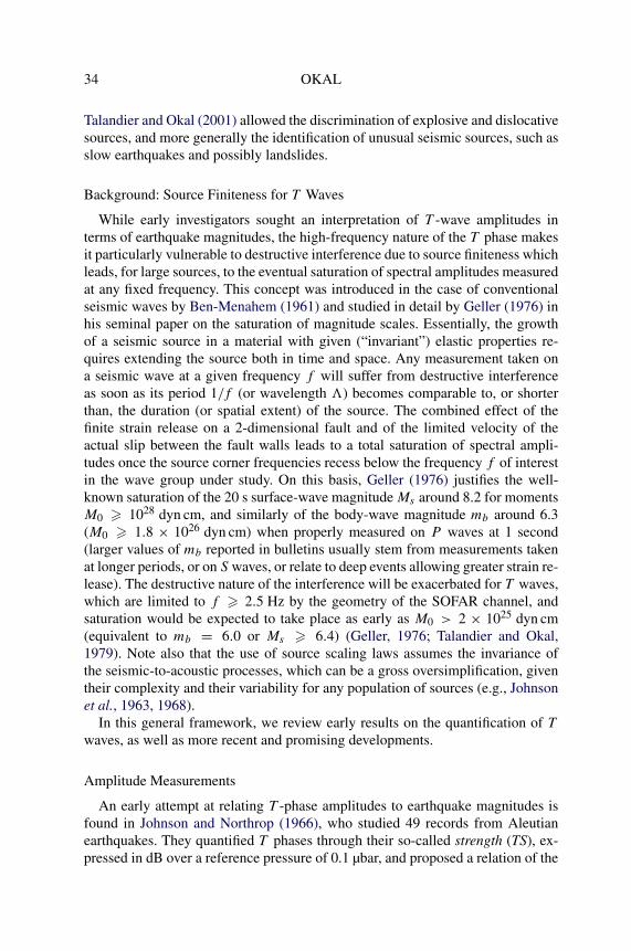
An early attempt at relating T -phase amplitudes to earthquake magnitudes isfound in Johnson and Northrop (1966), who studied 49 records from Aleutianearthquakes. They quantified T phases through their so-called strength (TS), ex-pressed in dB over a reference pressure of 0.1 µbar, and proposed a relation of the

THE GENERATION OF T WAVES BY EARTHQUAKES 35
FIG. 15. Examples of correlation between earthquake magnitude and T -phase amplitudes.(a): Correlation with T -phase strength after Johnson and Northrop (1966). In (b), the same datasetis fit by least-squares. Note the mediocre correlation coefficient, and the much reduced slope, whenthe latter is left to float; the dashed line reproduces the regression proposed in (a). (c): Correlation withsurface-wave magnitude for 24 East Pacific Rise earthquakes (Yang and Forsyth, 2003). This diagramhas been replotted using the exact the same orientation and scales as in (a) and (b). Note the much im-proved correlation. Combination (re-labeled, rotated, combined) of new material (b) and material (a)from Johnson and Northrop (1966), and (c) from Yang and Forsyth (2003).
form
(4)TS = 20M − 52 (Fig. 15a).
However, this approach has several shortcomings. First, the constant 20 wasfixed, under the assumption that the T -phase amplitude should parallel seismic

36 OKAL
amplitude; second, it is not clear which magnitude (mb; Ms) is used in (4).We conducted an independent regression of Johnson and Northrop’s (1966)dataset allowing the slope to float (Fig. 15b), which yields a much gentler slope:TS = 10.59M − 8.60, but a mediocre correlation coefficient of only 0.47. Thislower value of the best-fitting slope indicates that T -phase amplitudes are indeedaffected by destructive interference in a range of magnitudes where Ms (and prob-ably mb) should not be. Fox et al. (2001) also reported a lower value (7.84±2.04)of the slope of acoustic source level (in dB) vs. mb for a dataset of 87 eventsrecorded at the Autonomous Equatorial Array. Such results are also in agreementwith those of Yang and Forsyth (2003), reproduced on Fig. 15c, who regress theamplitude AT of T phases as log10 AT = 0.49Ms − 0.72 (equivalent to a slopeof 9.8 between TS and Ms in (4)) for a very homogeneous dataset of 24 East Pa-cific Rise earthquakes at regional distances. The factor 0.49 similarly expressesthat T -wave amplitudes do suffer from interference effects in a range of magni-tudes (Ms � 5) where 20-second waves are immune from them.
Walker et al. (1992) later investigated the correlation of T -phase strength(which they restricted to the frequency range 10–35 Hz) with seismic moment M0for a dataset of 25 Pacific-rim earthquakes recorded at the Wake hydrophone ar-ray. The use of M0 should ensure a more robust estimation of the true size oflarge events, and Walker et al. (1992) indeed observe an excellent correlation forcertain sub-datasets (their Fig. 17), but their results are difficult to interpret sincemost of their large moments involve strike–slip sources in the Gulf of Alaska; asdiscussed below, this geometry may be a preferential T -phase generator (Dziak,2001), and those strike–slip earthquakes may thus not be directly comparable tothe remainder of the dataset, consisting almost exclusively of thrust and normalevents. Hiyoshi et al. (1992) similarly studied 17 Japanese earthquakes recordedat Wake. They observe a strong correlation between TS and log10 M0, but the re-sulting slopes are only half of those suggested by Walker et al. (1992), and theearthquakes in their dataset are generally smaller.
Duration: Another Measure of Source Size
As source size is increased, so is the time it takes for the rupture to take placeat any given point on the fault, and more significantly to propagate along the fullextent of the fault zone. As a result, scaling laws predict that the duration of anyseismic wavetrain should also grow, in principle linearly with the dimension of thesource, or like M
1/30 . This idea forms the basis of the use of duration magnitudes
(e.g., Lee et al., 1972; Real and Teng, 1973), and it would be expected that theduration of T waves should also grow with source size.
Indeed, a number of early studies sought to measure the duration of the T phaseof large shocks in relation to their size. Eaton et al. (1961) noted that the T phaseof the 1960 Chilean earthquake lasted as much as 6 minutes, while Ben-Menahem

THE GENERATION OF T WAVES BY EARTHQUAKES 37
and Toksöz (1963) proposed 4 minutes for the 1958 Fairweather, Alaska earth-quake. However, neither of these authors gave a formal definition of duration.Following an idea suggested by Johnson (1970), Okal and Talandier (1986) an-alyzed a large dataset of T waves from Pacific shocks recorded in Tahiti andHawaii, and obtained reasonable correlations between their durations and vari-ous magnitude scales. They defined the duration of the wavetrain either as thatof sustained maximum amplitude, or that of saturation on paper records at Poly-nesian stations. In particular, they showed that T -wave duration keeps growingwith seismic moment, even for the very largest seismic events (Alaska, 1964;Chile, 1960). Consequently, Okal and Talandier (1986) suggested the use of T -phase duration as an indicator of the tsunamigenic potential of large earthquakes,with a threshold of 100 s for the excitation of a destructive transoceanic tsunami(M0 � 5 × 1028 dyn cm). They noted, however, the presence of outliers in theirdataset, notably strike–slip earthquakes on the Alaskan Fairweather Fault.
T -Phase Energy Flux: The Parameter γ
In an attempt to characterize the total energy generated by an earthquake sourceinto a T wave, Okal et al. (2003) introduced the concept of the T -Phase EnergyFlux (TPEF), which mimics the estimated energy EE developed by Newman andOkal (1998) for body waves. The latter was itself inspired by Boatwright andChoy’s (1986) algorithm for the computation of radiated seismic energy, but withthe philosophy of a magnitude measurement, i.e., a real-time “quick-and-dirty”single-station estimate ignoring such source details as focal geometry and exactdepth.
Specifically, given a seismic record of the vertical ground motion u(t) of a T
phase, Okal et al. (2003) define
(5)TPEF = ρα
∫W
[u(t)
]2 dt,
where ρ and α are the density and P -wave velocity of the receiver medium, and W
is an appropriate time window containing the T phase. Using Parseval’s theorem,TPEF can be more readily computed in the Fourier domain as
(6)TPEF = ρα
π
∫ ωmax
ωmin
ω2∣∣U(ω)
∣∣2 dω,
where the spectral amplitude U(ω) is the Fourier transform of u(t), and ωmin andωmax are adequate bounds expressing the natural filtering resulting from propaga-tion in the SOFAR channel and seismic recording.
Because of the complexity of the conversion mechanisms near the source andreceiver, it is not possible to derive a universal correction and to interpret TPEF interms of the absolute energy radiated by the source into the T phase. Also, sucha correction would require a full understanding of the response of the receiving

38 OKAL
FIG. 16. Correlation between seismic moment M0 and TPEF, as recorded at Rarotonga for earth-quakes along a 250-km stretch of the coast of Central Chile (solid dots). The dotted line, with a slopeof 0.74, is the best linear regression of the dataset of 7 points. The solid line, with a slope constrainedto 1, defines the best-fitting value of γ (1.40). The two open squares show the large 1996 Nazca event,and one of its strong aftershocks; note that the best regression (dash-dot line, with a slope of 0.79)and the best-fitting γ (1.48; long dashes) are essentially unchanged, even though the new events arelocated in Peru, more than 1000 km away from the original seven. By contrast, the 1996 Chimbote“tsunami earthquake” (triangle) features an extreme deficiency in TPEF of two logarithmic units in γ ,or about six times the scatter in the Chilean data. Adapted (re-labeled) from (Okal et al., 2003).
shore to an acoustic wavetrain, and could therefore depend on such parameters asthe back-azimuth of the wavetrain at the station. For this reason, Okal et al. (2003)limit the scope of the parameter TPEF to the comparison of records obtained at thesame station under equivalent receiving conditions, i.e., from similar epicentralareas. In particular, no distance correction is applied in (6).
As in the case of body waves, the quantity TPEF would then be expected toscale linearly with seismic moment M0 and thus the parameter � = TPEF/M0
to remain invariant for sets of comparable seismic sources. (To avoid the use ofexceedingly small numbers, we further introduce γ = log10 � + 30, where � isin cm−2.)
This is verified on Fig.16 which examines the relationship between TPEF andM0 for ten South American earthquakes recorded at Rarotonga. Note the gen-erally good agreement between the two parameters, suggesting a constant γ ,the only earthquake exhibiting a pronounced deficiency in γ (by 1.5 logarith-mic units) being the 1996 Chimbote, Peru, “tsunami earthquake”. We recall that

THE GENERATION OF T WAVES BY EARTHQUAKES 39
Kanamori (1972) defined “tsunami earthquakes” as those events whose tsunamisare much larger than expected from their conventional magnitudes, typical exam-ples being the 1896 Sanriku, 1946 Aleutian, 1975 Kuriles and more recently, 1992Nicaraguan earthquakes. These have been shown to feature an extremely slowpropagation of the rupture along the fault plane, at velocities as low as 1 km/s,itself interpreted as involving rupture in sedimentary wedges (as proposed forSanriku (Tanioka and Satake, 1996) or Kuriles (Fukao, 1979)), or conversely ina jerky mode along a corrugated fault plane, in the case of a sediment-starvedenvironment such as Nicaragua (Tanioka et al., 1997; Polet and Kanamori, 2000).
The clear violation of source scaling laws by “tsunami earthquakes” is illus-trated by their strong mb : Ms anomalies, recast in more quantitative terms byNewman and Okal (1998) as a deficiency of more than 1 logarithmic unit in theslowness parameter = log10[EE/M0]. Such a source slowness is expected toaffect the parameter γ as well, and Okal et al. (2003) documented that all tsunamiearthquakes are strongly deficient generators of T waves, by comparing them withregular events located in the same general area (Fig. 17). The case of the tsunamiearthquakes of the 1990s (Nicaragua, 1992; Chimbote, Peru, 1996) for whichhigh-quality digital records are available, is most compelling (γ deficient by anaverage of 1.8 and 1.7 logarithmic units, respectively), but the technique can beextended to analog records in the case of the 1963 Kuriles main aftershock, 1975Kuriles earthquake and 1982 Tonga event, all of which were described as “tsunamiearthquakes” (Fukao, 1979; Talandier and Okal, 1989). Also, Okal et al. (2003)and Okal (2004) showed that a faint T wave detected at Hawaii Volcano Obser-vatory in the aftermath of the 1946 Aleutian earthquake arrived too late to beassociated with the main shock, and thus confirmed that the latter had not gener-ated a detectable T phase, which further supports its character as an exceptionallyslow tsunami earthquake (Kanamori, 1972; López and Okal, 2006).
These results settled a controversy regarding the correlation between T -phaseexcitation and the tsunamigenic character of an earthquake source, which hadbeen longstanding ever since Ewing et al. (1950) suggested the use of T phasesin tsunami warning, based on the assumption that both kinds of waves wouldbe favored by a very shallow seismic source involving strong coupling with theoceanic column. While their model was disputed by Leet (1951) and Wadati andInouye (1953), Talandier (1966) and later Walker et al. (1992) and Walker andBernard (1993) have supported the proposed correlation. However, such studieswere mostly based on restricted datasets, and predated the large tsunamis of the1990s, and in particular the “tsunami earthquakes” of 1992 (Nicaragua), 1994(Java) and 1996 (Chimbote, Peru). As mentioned above, modern developmentshave rendered Ewing et al.’s (1950) model precarious since we now understandthat T waves can be generated by the very deepest events (Northrop, 1974; Okal,2001b), while the generation of far-field tsunami energy is only mildly controlledby source depth for reasonably shallow earthquakes (h � 70 km) (Ward, 1980;Okal, 1988). In addition, Ewing et al. (1950) were simply overlooking the extreme

40O
KA
L
FIG. 17. Comparison of T phases from the Chimbote, Peru “tsunami earthquake” of 21 February 1996 (M0 = 2.2×1027 dyn cm; top frames) and the regularNazca, Peru event of 12 November 1996 (M0 = 4.6 × 1027 dyn cm; bottom frames). Vertical scales (in digital units) are arbitrary, but for each station (RAR:Rarotonga, Cook Is.; RPN: Rapa Nui, Easter Is.; RKT: Rikitea, Gambier; PATS: Pohnpei, Caroline Is.), the two T wavetrains are plotted on the same scale. Thestrong deficiency of the Chimbote T waves is quantified by the difference in the parameters γ of the two events at each station. Adapted (re-labeled) from (Okalet al., 2003).

TH
EG
EN
ER
AT
ION
OF
TW
AV
ES
BY
EA
RT
HQ
UA
KE
S41
FIG. 17. Continued.

42 OKAL
and fundamental difference in the frequencies characteristic of the two typesof waves. Indeed, the most efficient tsunami generators, the so-called “tsunamiearthquakes”, are essentially silent in the acoustic band, just as they often haveminimum amplitudes at 1 Hz. As a result, they can remain unfelt by the local resi-dents, who then lack any harbinger of the upcoming disaster, and do not realize theneed to urgently evacuate beaches. Such was the tragic case in Nicaragua (1992)where the tsunami killed more than 160 people (Satake et al., 1993), and in Java(1994 and 2006), where the human toll reached 223 and about 700, respectively(Tsuji et al., 1995, Fritz et al., 2007).
The failure of the proposed correlation between the excitation of tsunamisand T waves is further illustrated by the fact that those few earthquakes whoseT waves were actually felt at teleseismic distances in the Pacific Basin (the 1958Fairweather, Alaska, 1977 Tonga, 1994 deep Bolivian and 2003 New Zealandearthquakes; see above) all had at most weak teleseismic tsunamis, while the ma-jor catastrophic transpacific tsunamis (1946 Aleutian; 1960 Chile) were not, toour knowledge, accompanied by T waves of sufficient amplitude to be felt in thefar field. The 2004 Sumatra T waves were felt in the Maldives, at comparativelyshort distances.
In conclusion, the concept of the TPEF and the associated parameter γ can be apowerful tool for the investigation of the dynamic properties of a seismic source.In particular, it proves the deficiency of tsunami earthquakes as T -phase genera-tors and establishes firmly this property in the context of seismic source theory, byinvoking rupture slowness, itself resulting in a deviation from generally acceptedsource scaling laws. TPEF and hence γ involve straightforward, one-station mea-surements which can be carried out in real time in an observatory environment,and offer immediate insight into the dynamic properties of the source of a distantearthquake.
The Amplitude-Duration Criterion D
In a recent contribution, Talandier and Okal (2001) introduced a source dis-criminant D comparing the duration and amplitude of teleseismic T wavetrainsrecorded at island stations. In the context of the monitoring of the CTBT, theirmotivation was primarily to devise a robust algorithm capable of discriminatingbetween explosive sources in the water column and elastic dislocations in the solidEarth. Specifically, and given the time series x(t) of the ground velocity recordedby a seismic station, they characterize its amplitude through the maximum, eMax,expressed in µm/s, of the envelope e(t) of x(t), after high-pass filtering x above2 Hz. The duration τ1/3 of the wavetrain is taken as the total time (in s) duringwhich the envelope e(t) maintains a value of at least 1
3eMax (Fig. 18). The dis-criminant D is then computed as
(7)D = log10 eMax − 4.9 log10 τ1/3 + 4.1.

THE GENERATION OF T WAVES BY EARTHQUAKES 43
FIG. 18. Computation of the source discriminant D illustrated in the case of the Polynesian nucleartest of 27 January 1996, recorded at Rarotonga. (a): Original broad-band seismogram. (b): Seismogramhigh-pass filtered at 2 Hz. The thick trace represents the envelope of the record, whose maximumamplitude eMax is retained. The thick horizontal segments identify those time intervals during whichthe envelope is sustained at 1/3 of its maximum value (estimated above ambient noise); their totalduration is summed to obtain τ1/3. Finally, the discriminant D is computed using (7).
Figure 19 shows that D effectively separates most earthquakes (D < 0) from doc-umented explosions (D > 0).
In developing this discriminant, Talandier and Okal (2001) were motivated bythe failure of several other techniques, applied either in the time or frequencydomains, to adequately separate populations of earthquakes and underwater ex-plosions. By comparing an instantaneous measurement (the envelope maximumeMax) and an integrated one (the duration τ1/3), they contrast the high- and low-frequency properties of the source, in a way reminiscent of the time-honoredmb : Ms discriminant used to identify underground explosions based on theirclassical seismic waves (Marshall and Basham, 1972).
In order to justify the performance of the discriminant D, Talandier and Okal(2001) have discussed in very general terms the scaling laws governing the growthwith source size of underground dislocations and underwater explosions, and theresulting differences in the power laws controlling the duration and amplitude

44 OKAL
FIG. 19. Performance of the discriminant D (Eq. (7)) for the initial dataset of 105 records at atollstations studied by Talandier and Okal (2001). The dashed line separates positive and negative valuesof D. Note that all chemical explosions in the oceanic column (triangles) have positive D, while mostearthquakes (circles) feature negative discriminants. The exceptions (shown as bull’s eye symbols)involve two small earthquakes originating in the Hawaiian volcanic structure; see text for details.Adapted (re-labeled) from Talandier and Okal (2001).
of the acoustic wave generated in the SOFAR channel, which indeed lead to apredictable separation of the two populations in the eMax : τ1/3 plane for largeenough sources (magnitude mb � 2 or yield Y � 10 kg).

THE GENERATION OF T WAVES BY EARTHQUAKES 45
We refer to Talandier and Okal (2001) for a full discussion of the operationaldetails of the algorithm, notably regarding the definition of a necessary distancecorrection, the handling of background noise, the optimization (by trial and error)of the factor 1/3 for the definition of duration, and the preferential use of receivingstations located either on atolls or in the vicinity of a steep, “pali”-like, conversionzone, in order to prevent a long receiver-side upslope conversion from lengtheningthe wavetrain and diminishing its amplitude.
An important feature of Fig. 19 is the observation that, while documentedexplosions are well identified by the parameter D, the performance of the dis-criminant is degraded for a small number of earthquakes occurring in the vicinityof intraplate volcanic edifices, such as Hawaii (and Mehetia in the Society Is-lands), and dubbed “hotspot earthquakes”. These events feature an essentiallynull, or even slightly positive, value of D, which Talandier and Okal (2001) ex-plain by noting that, for small earthquakes occurring in the immediate vicinity ofthe source-side conversion point, the ground motion giving rise to the acousticwave may belong to the seismological near field, rather than to the far field, andthus violate the scaling laws providing the basis for the discriminant D. Whilethis mis-identification of a few intraplate earthquakes may appear as a failure ofthe proposed discriminant, it actually shows that D is a powerful proxy for thecharacteristics of T -wave sources, and suggests its use to explore systematicallythe source properties of certain classes of earthquakes.
Note also on Fig. 19 that D fails to identify T -phase sources documented asbelonging to episodes of underwater volcanic activity. This merely reflects thebroad variability of the nature of these sources during the course of a volcaniceruption (e.g., Talandier and Okal, 1987). These may include explosive events,corresponding to the initial unplugging of magmatic conduits, which not surpris-ingly can share the characteristics of underwater explosions and feature positivevalues of D, as well as slower phenomena occurring later in the sequence andassociated with the progression of magma within the conduit and its delivery tothe ocean floor; the latter can then feature some of the most negative values of D
in Talandier and Okal’s (2001) dataset.Talandier and Okal (2004b) recently complemented their initial study by sub-
stantially enlarging their dataset through inclusion of specially targeted familiesof sources. Among their most significant results, they confirmed the special be-havior of many, but not all, “hotspot earthquakes” which show enhanced valuesof the discriminant D (Fig. 20a). They were able to associate those records featur-ing positive D with sources in the immediate vicinity of steep conversion zones,which provide an efficient conversion resulting in high amplitudes and short du-rations.
By contrast, Talandier and Okal (2004b) studied 10 records from true intra-plate earthquakes, located in abyssal areas where no significant bathymetry isdocumented. They all feature negative values of D, and are thus unequivocallyidentified as earthquakes (Fig. 20b). These include some of the most negative D

46 OKAL
FIG. 20. Discriminant D applied to intraplate earthquakes located inside (or close to) volcanicedifices (“Hotspot earthquakes”; (a): open circles) or in abyssal plains with no known bathymetricfeatures (“True intraplate”; (b): downward-pointing triangles). The background symbols in half-toneare the original dataset from Talandier and Okal (2001). D = 0 is shown as the dashed line. Notethe occasional positive values of D for hotspot earthquakes, corresponding to sources located closeto steep slopes in the volcanic edifice. By contrast, the true intraplate earthquakes all have negativevalues of D, some of them among the lowest measured. After Talandier and Okal (2004b).
values in the authors’ catalogue, which expresses the general inefficiency of thescattering mechanisms required for abyssal conversion, especially at the relativelylow acoustic frequencies typical of seismic recording. In addition, the delocal-ization of the scatterers on the ocean floor can contribute to an increase in theduration of the signal, as modeled by deGroot-Hedlin and Orcutt (1999) and Yangand Forsyth (2003). The occasionally larger but still negative values of D shownon Fig. 20b could result from conversions involving an unchartered bathymetricfeature.
Figure 21 further compares the properties of T waves generated from earth-quakes at the subduction zones of the Pacific “Ring of Fire” and along transformfaults of the Pacific Mid-Oceanic Ridge systems. While the average value of D isslightly greater for the latter, there is no clear separation of the two populations.Anomalous events, featuring normal faulting on the Eltanin Transform Faults(Okal and Langenhorst, 2000), are not identifiable within the group. On the otherhand, this dataset does support the observation that strike–slip earthquakes (fromthe Transform Fault dataset) may be nominally more efficient T -wave generatorsthan thrust or normal faulting ones, especially at lower magnitudes. Figure 22

THE GENERATION OF T WAVES BY EARTHQUAKES 47
FIG. 21. Comparison of the performance of the discriminant D for 35 records from earthquakeson transform faults ((a): left-pointing triangles) and 53 records of subduction zone events ((b): solidcircles). The background symbols in half-tone are the original dataset from Talandier and Okal (2001).D = 0 is shown as the dashed line. After Talandier and Okal (2004b).
(Talandier and Okal, 2004b) documents and quantifies this trend on a popula-tion of 23 T phases recorded at Rarotonga from the Eltanin and Kurile epicentralareas. These results are generally compatible with those of Dziak (2001), whohad first reported this property using hydrophone records of regional events inthe area of the Juan de Fuca and Gorda Ridges (Fig. 22a). While the trends ofthe two datasets are largely similar, the slopes of the best-fitting regressions dif-fer significantly. However, in Talandier and Okal’s (2004b) study, the regressionslopes had to be computed using body-wave magnitude mb in the absence of asufficient number of published moment values, whereas Dziak (2001) used mo-ment magnitudes obtained by inversion of regional waveforms (Nábelek and Xia,1995). In the relevant range of magnitudes, the slope of mb vs. log10 M0 is ex-pected to vary between 2/3 (mb � 5) and 1/3 (mb > 5) (Geller, 1976), andconsequently, Talandier and Okal’s (2004b) slopes should be adjusted by a factorwhich could reach 0.5, in order to be compared with those of Dziak (2001). Addi-tional differences between the two studies may reflect the variation in frequencyband resulting from the difference in instrumentation.
Park et al. (2001) have suggested that the preferential excitation of T wavesby strike–slip faults may express the dependence of Rayleigh wave excitation onfocal mechanism and depth (e.g., Kanamori and Stewart, 1976). A simple physi-

48 OKAL
cal analysis of this conjecture is not forthcoming, as the extremely short seismicwavelengths involved (i.e., the very large equivalent angular orders in the spheri-cal Earth, on the order of l = 104 to 105 for the modes on Fig. 10) preclude the useof asymptotic expansions valid for shallow sources or in the limit of the seismicnear field; note in particular that the scatterers are bound to range several, if notmany, wavelengths away from the epicenter. In addition, the apparent decrease ofthe effect with earthquake size, recognizable in both Dziak’s (2001) and Talandierand Okal’s (2004b) datasets (Fig. 22), would suggest that source finiteness playsa crucial role; however, its effect on the excitation of seismic surface waves doesnot lend itself to a simple analysis at very high frequencies, both in the directiv-ity formalism (Ben-Menahem, 1961) or the higher-moment one (Okal, 1982). Bycontrast, the formalism of Yang and Forsyth (2003) may, at least conceptually,be more directly applicable to further exploring the effect of focal mechanism onthe generation of abyssal T waves; at any rate, it is clear that more systematictheoretical investigations will be necessary before the origin of this remarkableobservation is fully understood.
Talandier and Okal (2004b) also explored the T -wave characteristics of un-derwater landslides, by considering the case of the Papua New Guinea (PNG)earthquake series of 1998 (Fig. 23). We recall that a major local tsunami, whichkilled more than 2200 people, was generated following a relatively weak earth-quake (M0 = 3.7 × 1026 dyn cm), which did not feature the slow character of“tsunami earthquakes” (Synolakis et al., 2002). The origin of the tsunami waslater attributed to an underwater landslide, triggered 13 minutes after the main-shock and identified from its T wave recorded throughout the Pacific Basin, andin particular on the Wake Island hydrophone (Okal, 2003). The T waveform wasexceptionally long, given the small classical magnitude (mb = 4.4) assigned to itssource. This can be interpreted as a disparity between amplitude and duration ofthe source, which we formally examine on Fig. 23, where we plot D values com-puted from waveforms recorded at the seismic station on Wake Island. In additionto the tsunamigenic slump (with origin time 09:02 GMT on 17 July 1998), thedataset on that figure consists of the 1998 PNG mainshock (08:49), of a numberof small aftershocks (09:06, 09:40), and of the mainshock of the 2002 PNG event,which occurred 120 km to the Southeast, was larger than the 1998 earthquake, butgenerated only a benign tsunami (Borrero et al., 2003). Note that the 09:02 event(D = −3.55) effectively features a deficiency in D of more than one logarithmicunit with respect to most of the neighboring events, suggesting a source processof a different physical nature. By contrast, the 1998 and 2002 mainshocks featurecomparable values of D (−1.58 and −1.26 respectively), supporting a common-ality of seismic source, which again requires that the catastrophic 1998 tsunamimust have been generated by an auxiliary source.
In addition, we point out a small event on 12 December 2002, located 6 km offthe southwestern shore of the Island of Hawaii, and featuring D = −3.18. Whilethis value is not significantly different from those of truly intraplate earthquakes,

THE GENERATION OF T WAVES BY EARTHQUAKES 49
FIG. 22. Preferential excitation of T waves by strike–slip earthquakes. (a): Dziak’s (2001) datasetof 179 regional earthquakes recorded on hydrophones in the Northeast Pacific. The regression slopeshave been reinterpreted in terms of linear physical units, rather than decibels, as 0.25 (strike–slip)and 0.38 (other), (b): Talandier and Okal’s (2004b) dataset of 8 T phases from subduction eventsin the Kuriles (open symbols; regressed as dashed line), and 15 transform fault earthquakes fromthe Eltanin Fracture Zone (solid symbols; regressed as solid line), recorded at Rarotonga. Note thegenerally similar pattern of preferential excitation of T phases by the latter at low magnitudes. Seetext for discussion. Combination of new material with figure adapted from Dziak (2001).

50 OKAL
FIG. 23. Discriminant D computed at the Wake Island seismic station for a series of events inPapua New Guinea on 17 July 1998. Note that the 09:02 aftershock, interpreted as a major underwaterslump (Synolakis et al., 2002), features a deficit of more than one unit (D = −3.55) with respect toneighboring earthquakes. Also shown are the regular event nearby on 08 September 2002, and a small2002 event near the coast of Hawaii interpreted by Reymond et al. (2004) as an underwater landslide.The background symbols in half-tone are the original dataset from Talandier and Okal (2001). D = 0is shown as the dashed line. After Talandier and Okal (2004b).
it is substantially deficient among Hawaiian earthquakes, and reminiscent of thatof the 1998 PNG underwater landslide. This observation, and the comparison ofthe regional seismic waveforms recorded on the island with those of documentedsubaerial landslides, suggests that the event in question is indeed an underwaterlandslide, taking place on a steeply sloping section of the island structure identifi-able in the local bathymetry (Reymond et al., 2004). This tentative interpretationwould support the contention that landslides are probably rather inefficient, if notoccasionally silent, sources of hydroacoustic energy, even though their durationmay be substantial. Incidentally, such signals differ significantly from those de-scribed by Caplan-Auerbach et al. (2001) as originating from bench collapses

THE GENERATION OF T WAVES BY EARTHQUAKES 51
at the Kilauea eruption ocean entry point and recorded on hydrophones of theautonomous equatorial array (Fox et al., 2001). The latter have much shorter du-rations, which probably reflects the difference in the nature of the slide (the simplecollapse of a cohesive block) and the shorter length of its total underwater path.
Finally, in Fig. 24, we compare on a dataset of eight South American earth-quakes the performance of the three parameters D, γ , and , introduced byTalandier and Okal (2001), Okal et al. (2003) and Newman and Okal (1998) todetect any possible slowness in the rupture characteristics of seismic sources. Thefirst two are based on the properties of T waves, and the third one on the energyof body waves. The eight events span two logarithmic units of , including bothslow earthquakes such as the 1996 Chimbote, Peru “tsunami earthquake”, and fastor “snappy” ones such as the Chilean event of 15 October 1997 (Okal and Kirby,2002). We find remarkable correlations between γ and (86%), and between D
and γ (84%), and a spectacular one (98%) between D and . In particular, the1996 Chimbote, Peru earthquake features the lowest value of D (−7.03) mea-sured by Talandier and Okal (2004b). The 2001 Peruvian mainshock, identifiedas trending toward slowness (Okal et al., 2002) also features a low value of D,and to a lesser extent, of γ . By contrast, all three “snappy” earthquakes with largevalues of also have high parameters γ and D. These include the two deeperthan normal intraplate events in Chile and the normal faulting Peruvian shocktriggered on 05 July 2001 by stress transfer from the Peruvian mainshock.
These observations serve to confirm, if need be, that D can be a reliable descrip-tor of the source properties of an earthquake, and more generally that the T -phasewaveform carries valuable information on the source properties of earthquakes,which can be extracted through the use of analytical algorithms paralleling themethodologies traditionally utilized on conventional seismic waves.
The Case of the 2004 Sumatra Earthquake
With a seismic moment of at least 1030 dyn cm (Stein and Okal, 2005; Tsaiet al., 2005), the disastrous Sumatra–Andaman earthquake of 26 December 2004was the largest one in 40, and perhaps 44, years. A fascinating aspect of this eventis that its recordings transcended the conventional boundaries of instrumentation.For example, its tsunami was recorded by technologies as diverse as satellite al-timetry (Scharroo et al., 2005), infrasound (Le Pichon et al., 2005), hydrophonesof the International Monitoring System (IMS) of the CTBT Organization (Hansonand Bowman, 2005), detection of ionospheric perturbation using arrays of GPSrecorders (Occhipinti et al., 2005), and even on the horizontal components ofnear-shore broadband seismometers at teleseismic distances (Yuan et al., 2005;Okal, 2007). In this context, and given the unique character of the earthquake, adescription of its T waves is in order.
The source characteristics of the Sumatra earthquake were investigated in theframework of the parameters γ and D introduced above. In this respect, we recall

52 OKAL
Number Date Event Remarks
1 1966:052 Chimbote, Peru Tsunami Earthquake2 1996:317 Nazca, Peru3 2001:174 Peru, Main shock4 2001:177 Peru, First Large Aftershock5 2001:186 Peru, Triggered Normal Faulting Snappy6 2001:188 Peru, Largest Aftershock7 1997:288 Ovalle, Chile Snappy (Okal and Kirby, 2002)8 1998:210 Chile (Outboard, Intraplate) Snappy
FIG. 24. Correlation between various scale-invariant measures of the slowness of an earthquakesource, investigated on T wave records at Rarotonga of eight South American earthquakes, listed in thebox. Top: Parameter γ vs. slowness parameter introduced by Newman and Okal (1998). Center left:Discriminant D vs parameter γ . Center right: Discriminant D vs. . Note the excellent correlations,especially in the latter case. See text for detailed interpretation.

THE GENERATION OF T WAVES BY EARTHQUAKES 53
FIG. 25. Top: Map of the Northeastern Indian Ocean Basin showing the 2004 and 2005 Sumatraevents (stars) and paths of T phases to the Maldives and Diego Garcia, with partial rays to Crozet(H04) and Cape Leeuwin (H01). The small symbols represent the same-day aftershocks of the 2004Sumatra earthquake, and illustrate the extent of the fault rupture. Bottom: Accelerogram of the T phasedeconvolved from the broadband seismometer record at the seismic station DGAR on Diego Garcia.Note that the duration of the record does not extend beyond 450 seconds.
that only relative evaluations at the same receiver are legitimate, and proceed tocompare the T wavetrains recorded at the seismic station DGAR on Diego Gar-cia atoll from the 2004 Sumatra–Andaman earthquake and the Simeulue–Niasevent of 28 March 2005 to the Southeast (Fig. 25). At M0 = 1.1 × 1029 dyn cm,the latter, apparently triggered by Coulomb stress transfer from the 2004 event

54 OKAL
FIG. 26. Analysis of T phases recorded at the seismic station DGAR (Diego Garcia) from the twolarge 2004 and 2005 Sumatra earthquakes. Top: Broadband seismograms high-pass filtered at 2 Hz(yielding essentially ground velocity) plotted on common time and amplitude scales, with parame-ters relevant to the calculation of TPEF and γ . Bottom: Calculation of the discriminant D. Note therelatively comparable values of eMax, but the very much longer τ1/3 in the case of the 2004 event,resulting in a much lower value of D.
(McCloskey et al., 2005) is itself truly gigantic, and would have been the largestrecorded event since 1965, if not for the 2004 Sumatra earthquake. Figure 26compares the relevant waveforms and demonstrates a significant difference (ofmore than two units) in the discriminants D. Note that the Northern extremityof the 2004 rupture is generally masked in the direction of Diego Garcia, result-ing in a somewhat shortened T wave, not exceeding 450 s in duration (Fig. 25),

THE GENERATION OF T WAVES BY EARTHQUAKES 55
FIG. 27. Source tomography of the 2004 Sumatra earthquake. Top: Time history of the progressionof the rupture along the fault line as mapped by backtracking beamed signals from Indian Oceanhydrophone arrays (deGroot-Hedlin, 2005). Bottom: Spaciotemporal evolution of the components ofthe multi-source CMT inversion of mantle waves by Tsai et al. (2005). The two diagrams use theexact same scales, allowing direct comparison. Note the remarkable agreement, especially regardingthe slowing down of the rupture to the North, and also the tentatively slow initiation of the rupturein the South. Adapted (combined; re-scaled; re-labeled) from deGroot-Hedlin (2005) and Tsai et al.(2005).
rather than the generally accepted value of at least 500 s obtained from seismicsource tomography (Ishii et al., 2005). This also results in an underestimationof τ1/3, which would suggest an even more deficient value of D. By contrast, theSimeulue–Nias 2005 earthquake featured bilateral rupture (Walker et al., 2005),resulting in an increased value of D. As for the parameters γ of the two events,they are found largely comparable.
T waves from the 2004 Sumatra earthquake were also recorded by hydrophonesof the IMS; by a stroke of luck, the deployment of the hydrophone part of the sys-

56 OKAL
tem started with the Indian Ocean sites, with stations operational in 2004 at DiegoGarcia (H08), Crozet (H04) and Cape Leeuwin (H01). The availability of triads ofhydrophones then allowed directional beaming of the signals using sophisticatedtechniques, like the PMCC method (Cansi, 1995), which tracks parameters suchas incident azimuth, frequency, signal strength and coherence among array sites,as a function of time in the wave packet. By back-tracking this information to thesource, T waves were successfully used in a series of studies (deGroot-Hedlin,2005; Guilbert et al., 2005; Tolstoy and Bohnenstiehl, 2005) to map the progres-sion of the acoustic source, and hence of the earthquake rupture along the faultplane, in what amounted to the first applications of T phases to detailed earth-quake source tomography. These studies confirmed the large spatial extent andlong duration of the source, and documented a generally slow, but subtly variable,rupture velocity (Fig. 27). Note that because of the slower propagation velocityof T waves in the ocean, hydroacoustic signals offer in this respect a better res-olution than comparable algorithms based on conventional body waves, such asused by Ishii et al. (2005) and Ohrnberger and Krüger (2005). The rupture veloc-ity (on the average 2.7 km/s) was found to be significantly deficient with respectto that predicted by scaling laws (typically 3.5 km/s), but without reaching thevery slow velocities, generally less than 2 km/s, typical of “tsunami earthquakes”(Polet and Kanamori, 2000; López and Okal, 2006). The emerging picture for the2004 Sumatra event is that of a definitive trend towards slowness, but falling shortof the truly anomalous behavior of the classic tsunami earthquakes, a propertyalso confirmed by Weinstein and Okal’s (2005) analysis of the parameter of the2004 earthquake.
In this context, it is interesting to note that tremors were reported widely feltin the Maldives around 06:30 local time (GMT + 5), which coincides with thepredicted arrival time of T waves. There was no seismic station operational onthe Maldives, but the T phases recorded at DGAR on Diego Garcia, 1530 km tothe South (Fig. 25), correspond to a maximum ground acceleration of 0.5 cm/s2.This is slightly below the generally accepted threshold for feeling by humans(1 cm/s2), but we note the unfavorable recording conditions at DGAR, where theseismic station faces the Southeastern shore, thus requiring a significant land pathfor the converted seismic wave. It is thus almost certain that the Sumatra T waveswere felt in the Maldives, four hours before the arrival of the tsunami, and in hind-sight that their correct interpretation could have led to a warning of the populationof this atoll nation, which suffered about 100 casualties. In this respect, the 2004Sumatra earthquake may be the only reported case of an earthquake having gen-erated a catastrophic oceanwide tsunami, and which had been felt in the far fieldthrough its T waves. The fact that the T waves were of high enough amplitude tobe felt is also consistent with the relatively high value of γ , relative to the 2005event: the 2004 earthquake did release significant amounts of high-frequency en-ergy which found its way into T waves, and it was anomalous only in that itssource lasted longer than expected, even for an event of its size. These remarks

THE GENERATION OF T WAVES BY EARTHQUAKES 57
further illustrate the different source characteristics controlling the parameters D
and γ .
6. CONCLUSION
In conclusion of this review, it is interesting to reflect on the role of earthquake-generated T phases in the development of hydroacoustics. Underwater explosionsobviously constitute simpler sources of acoustic energy in the ocean, and indeedhave been used in a broad range of calibration experiments, including Worzel andEwing’s (1948), Weigel’s (1990), and more recently Blackman et al.’s (2003).
However, the ubiquitous character of earthquake sources, both in space andtime, has made them the primary tool of the steady progress of our command ofhydroacoustics in the past 70 years. In this respect, and from the strict standpointof unclassified geophysical research, several eras emerge as milestones, whichcan be conveniently identified by the individual laboratories where the crucialdevelopments took place.
• The Lamont years (1950s), under the leadership of W. Maurice Ewing, sawthe emergence of the fundamental picture, establishing firmly the nature ofthe T wave and the relevant interactions between seismic and acoustic wavesat source and receiver slopes. The resulting model would pave the way for adecade of glorified applications of standard geometrical optics.
• The Hawaii years (1960s) involved the operation of a Pacific-wide arrayof hydrophones by the Hawaii Institute of Geophysics. Some of the mostfar-reaching results obtained by R.H. Johnson included the discovery ofMacdonald Seamount, and the identification of the limits of validity ofstrict geometrical optics. The dataset collected was truly massive by thosedays’ standards, and would fuel many years of seminal studies, notably byD.A. Walker, on various topical subjects. However, the 1970s and 1980s didnot see major developments in instrumentation.
• The PMEL years (1990s) resulted from partial declassification of SOSUS,which allowed C.G. Fox to detect and monitor in real time an episode ofvolcanic eruption on a segment of the Mid-Oceanic Ridge system. In turn,this led to the development and deployment of the autonomous arrays in thevicinity of the East Pacific in Mid-Atlantic Ridges.
• The 2000s should become the years of the International Monitoring System(IMS), as hydroacoustics were defined in 1996 as one of four technologiesto be used in the monitoring of the CTBT, which mandated the deploymentof six hydrophones and five land-based seismic T-phase stations. While hy-droacoustic monitoring is clearly aimed at the detection of man-made eventsin the water column, the growing database flowing from the IMS stations

58 OKAL
(and from other networks such as the autonomous arrays and the RSP) em-anates primarily from natural sources, some of which would not have beenenvisioned a decade ago, e.g., cryosignals generated by calving or driftingicebergs (Talandier et al., 2002, 2006). However, earthquakes remain a pre-mium source of hydroacoustic energy, and the new detection capabilitiesprovided by the implementation of the IMS will allow the furtherance ofour understanding of earthquake sources in the oceanic environment, no-tably through the use of the analytical methods being developed to interpretthe hydroacoustic spectrum in terms of source properties.
In this context, T waves are truly coming of age as an equal partner to conven-tional seismic waves.
ACKNOWLEDGEMENTS
I am grateful to Ralph Stephen and Robert Odom, conveners of the workshop on “Seismo-acoustic
applications in Marine Geology and Geophysics”, held at Woods Hole in March 2004, for inviting
me to present a keynote lecture, and encouraging me to write up a review paper on its topic. My
work on T phases has benefited from many years of regular cooperation with the Commissariat à
l’Energie Atomique (France), and particularly from joint research with Jacques Talandier, Dominique
Reymond and Olivier Hyvernaud. Several aspects of T -phase quantification were supported by the
Department of Defense, most recently under Contract DTRA01-00-C-0065, and regarding tsunami
hazard by the National Science Foundation, under Grant CMS-03-01054. I thank Library Staff at
Northwestern University, the University of Chicago and Harvard University for help with the retrieval
of historical references. Most maps were drafted using the GMT software (Wessel and Smith, 1991).
REFERENCES
Adams, R.D. (1979). T -phase recordings at Rarotonga from underground nuclear explosions. Geo-phys. J. Roy. Astr. Soc. 58, 361–369.
Bard, P.-Y., Campillo, M., Chavez-García, F.J., Sanchez-Sesma, F. (1988). The Mexico earthquake ofSeptember 19, 1985; A theoretical investigation of large- and small-scale amplification effects inthe Mexico City valley. Earthq. Spectra 4, 609–633.
Båth, M., Shahidi, M. (1971). T phases from Atlantic earthquakes. Pure Appl. Geophys. 92, 74–114.Ben-Menahem, A. (1961). Radiation of seismic surface waves from finite moving sources. Bull. Seis-
mol. Soc. Amer. 51, 401–435.Ben-Menahem, A., Toksöz, M.N. (1963). Source mechanism from spectra of long-period seismic
surface waves. 3. The Alaska earthquake of July 10, 1958. Bull. Seismol. Soc. Amer. 53, 905–919.Biot, M.A. (1952). The interaction of Rayleigh and Stoneley waves in the ocean bottom. Bull. Seismol.
Soc. Amer. 42, 81–93.Blackman, D.K., Mercer, J.A., Andrew, R., deGroot-Hedlin, C.D., Harben, P.E. (2003). Indian Ocean
Calibration tests: Cape Town–Cocos Keeling, 2003. In: Proc. 25th Seismic Res. Review – NuclearMonitoring: Building the Knowledge Base, Tucson, AZ, September 23–25, 2003, pp. 517–523.Nat. Nuclear Security Admin. (abstract).

THE GENERATION OF T WAVES BY EARTHQUAKES 59
Boatwright, J., Choy, G.L. (1986). Teleseismic estimates of the energy radiated by shallow earth-quakes. J. Geophys. Res. 91, 2095–2112.
Bohnenstiehl, D.R., Tolstoy, M., Dziak, R.P., Fox, C.G., Smith, D.K. (2002). Aftershock sequencesin the mid-ocean ridge environment: an analysis using hydroacoustic data. Tectonophysics 354,49–70.
Bohnenstiehl, D.R., Tolstoy, M., Smith, D.K., Fox, C.G., Dziak, R.P. (2003). Time-clustering behaviorof spreading-center seismicity between 15 and 35◦ N on the Mid-Atlantic Ridge: observationsfrom hydroacoustic monitoring. Phys. Earth Planet. Inter. 138, 147–161.
Borrero, J.C., Bu, J., Saiang, C., Uslu, B., Freckman, J., Gomer, B., Okal, E.A., Synolakis, C.E. (2003).Field survey and preliminary modeling of the Wewak, Papua New Guinea earthquake and tsunamiof September 9, 2002. Seismol. Res. Lett. 74, 393–405.
Brekhovskikh, L.M. (1949). O rasprostranenii zvuka v podvodnom zvukovom kanale. Dokl. Akad.Nauk SSSR 69, 157–160 (in Russian).
Brekhovskikh, L.M., Lysanov, Yu. (1982). Fundamentals of Ocean Acoustics. Springer-Verlag, Berlin,250 pp.
Brune, J.N. (1964). Travel times, body waves, and normal modes of the Earth. Bull. Seismol. Soc.Amer. 54, 2099–2128.
Butler, R., Lomnitz, C. (2002). Coupled seismoacoustic modes on the seafloor. Geophys. Res. Lett. 29(10), 571–574.
Cansi, Y. (1995). An automatic seismic event processing for detection and location: The P.M.C.C.method. Geophys. Res. Lett. 22, 1021–1024.
Cansi, Y., Béthoux, N. (1985). T waves with long inland paths: Synthetic seismograms. J. Geophys.Res. 90, 5459–5465.
Caplan-Auerbach, J., Fox, C.G., Duennebier, F.K. (2001). Hydroacoustic detection of submarine land-slides on Kilauea Volcano. Geophys. Res. Lett. 28, 1811–1813.
Colladon, J.D., Sturm, J.K.F. (1827). La vitesse du son dans les liquides. Annales de Chimie et dePhysique, Série 2 36, 236–257.
Collins, M.P. (1936). Bulletin Number 5, Harvard University Seismograph Station, 5, 23 pp.Coulomb, J., Molard, P. (1949). Ondes séismiques au fond de la mer des Antilles. Ann. Geophys. 5,
212–214.Coulomb, J., Molard, P. (1952). Propagation des ondes séismiques T dans la mer des Antilles. Ann.
Géophys. 8, 264–266.deGroot-Hedlin, C.D. (2005). Estimation of the rupture length and velocity of the great Sumatra earth-
quake of Dec 26, 2004 using hydroacoustic signals. Geophys. Res. Lett. 32 (11), L11303, 4 pp.deGroot-Hedlin, C.D., Orcutt, J.A. (1999). Synthesis of earthquake-generated T waves. Geophys. Res.
Lett. 26, 1227–1230.Dietz, R.S., Sheehy, M.J. (1954). Transpacific detection of Myojin Volcanic eruptions by underwater
sound. Geol. Soc. Amer. Bull. 65, 942–956.Duennebier, F.K., Johnson, R.H. (1967). T -phase sources and earthquake epicenters in the Pacific
Basin, Hawaii Inst. Geophys. Rept. 67–24, Univ. Hawaii, Honolulu, 104 pp.Dziak, R.P. (2001). Empirical relationship of T -wave energy and fault parameters of Northeast Pacific
ocean earthquakes. Geophys. Res. Lett. 28, 2537–2540.Dziak, R.P., Fox, C.G., Schreiner, A.E. (1995). The June–July 1993 seismo-acoustic event at CoAxial
segment, Juan de Fuca Ridge: Evidence for a lateral dike injection. Geophys. Res. Lett. 22, 135–138.
Eaton, J.P., Richter, D.H., Ault, W.U. (1961). The tsunami of May 23, 1960 on the island of Hawaii.Bull. Seismol. Soc. Amer. 51, 135–157.
Embley, R.W., Chadwick Jr., W.W., Jonasson, I.R., Butterfield, D.A., Baker, E.T. (1995). Initial resultsof the rapid response to the 1993 CoAxial event: Relationships between hydrothermal and volcanicprocesses. Geophys. Res. Lett. 22, 143–146.
Ewing, W.M., Worzel, J.L. (1948). Long-range sound transmission. Geol. Soc. Amer. Mem. 27. Part 3,39 pp.

60 OKAL
Ewing, W.M., Woollard, G.P., Vine, A.C., Worzel, J.L. (1946). Recent results in submarine geo-physics. Geol. Soc. Amer. Bull. 57, 909–934.
Ewing, W.M., Tolstoy, I., Press, F. (1950). Proposed use of the T phase in tsunami warning systems.Bull. Seismol. Soc. Amer. 40, 53–58.
Ewing, W.M., Press, F., Worzel, J.L. (1952). Further study of the T phase. Bull. Seismol. Soc. Amer. 42,37–51.
Ewing, W.M., Jardetzky, W.S., Press, F. (1957). Elastic Waves in Layered Media. McGraw-Hill, NewYork, 380 pp.
Fischer, K.M., McCann, W.R. (1984). Velocity modeling and earthquake relocation in the NortheastCaribbean. Bull. Seismol. Soc. Amer. 74, 1249–1262.
Forsyth, D.W., Yang, Y., Mangriotis, M.-D., Shen, Y. (2003). Coupled seismic slip on adjacent oceanictransform faults. Geophys. Res. Lett. 30 (12), 201–204.
Fox, C.G., Dziak, R.P., Matsumoto, H., Schreiner, A.E. (1994). Potential for monitoring low-levelseismicity on the Juan de Fuca Ridge using military hydrophone arrays. Mar. Tech. Soc. J. 27 (4),22–30.
Fox, C.G., Radford, W.E., Dziak, R.P., Lau, T.-K., Matsumoto, H., Schreiner, A.E. (1995). Acousticdetection of a seafloor spreading episode on the Juan de Fuca Ridge using military hydrophonearrays. Geophys. Res. Lett. 22, 131–134.
Fox, C.G., Matsumoto, H., Lau, T.-K.A. (2001). Monitoring Pacific Ocean seismicity from an au-tonomous hydrophone array. J. Geophys. Res. 106, 4183–4206.
Fritz, H.M. and 17 co-authors (2007). Extreme runup from the 17 July 2006 Java tsunami. Geophys.Res. Lett. 34 (2), L12602, 5 p.
Fukao, Y. (1979). Tsunami earthquake and subduction processes near deep sea trenches. J. Geophys.Res. 84, 2303–2314.
Geller, R.J. (1976). Scaling relations for earthquake source parameters and magnitudes. Bull. Seismol.Soc. Amer. 66, 1501–1523.
Gilbert, F. (1970). Excitation of the normal modes of the Earth by earthquake sources. Geophys. J.Roy. Astr. Soc. 22, 223–226.
Guilbert, J., Vergoz, J., Schisselé, E., Roueff, A., Cansi, Y. (2005). Use of hydroacoustic and seismicarrays to observe rupture propagation and source extent of the Mw = 9.0 Sumatra earthquake.Geophys. Res. Lett. 32 (15), L15310, 5 pp.
Gutenberg, B. (1957). Effects of ground on earthquake motion. Bull. Seismol. Soc. Amer. 47, 221–250.Hammond, S.R., Walker, D.A. (1991). Ridge event detection: T -phase signals from the Juan de Fuca
spreading center. Mar. Geophys. Res. 13, 331–348.Hanson, J.A., Bowman, J.R. (2005). Dispersive and reflected tsunami signals from the 2004 In-
dian Ocean tsunami observed on hydrophones and seismic stations. Geophys. Res. Lett. 32 (17),L17608, 5 pp.
Harkrider, D.G. (1964). Surface waves in multilayered elastic media. Part I: Rayleigh and Love wavesfrom buried sources in a multilayered elastic half-space. Bull. Seismol. Soc. Amer. 54, 627–679.
Haskell, N.A. (1953). The dispersion of surface waves in multilayered media. Bull. Seismol. Soc.Amer. 43, 17–34.
Hiyoshi, Y., Walker, D.A., McCreery, C.S. (1992). T -phase data and regional tsunamigenesis in Japan.Bull. Seismol. Soc. Amer. 82, 2213–2223.
Isacks, B.L., Molnar, P. (1971). Distribution of stresses in the descending lithosphere from a globalsurvey of focal-mechanism solutions of mantle earthquakes. Rev. Geophys. Space Phys. 9, 103–174.
Ishii, M., Shearer, P., Houston, H., Vidale, J. (2005). Rupture extent, duration and speed of the 2004Sumatra–Andaman earthquake imaged by the Hi-Net array. Nature 435, 933–936.
Jaggar, T.A. (1930). How the seismograph works. The Volcano Letter 268, 1–4.Jensen, F.B., Kuperman, W.A., Porter, M.B., Schmidt, H. (1994). Computational Ocean Acoustics.
AIP Press, Woodbury, NY, 612 pp.
THE GENERATION OF T WAVES BY EARTHQUAKES 61
Johnson, R.H. (1970). Estimating earthquake rupture length from T waves. In: Adams, W.A. (Ed.),Tsunamis in the Pacific Ocean. Univ. Hawaii, Honolulu, pp. 253–259.
Johnson, R.H., Norris, R.A. (1968). T -phase radiators in the Western Aleutians. Bull. Seismol. Soc.Amer. 58, 1–10.
Johnson, R.H., Northrop, J. (1966). A comparison of earthquake magnitude with T-phase strength.Bull. Seismol. Soc. Amer. 56, 119–124.
Johnson, R.H., Northrop, J., Eppley, R. (1963). Sources of Pacific T phases. J. Geophys. Res. 68,4251–4260.
Johnson, R.H., Norris, R.A., Duennebier, F.K. (1968). Abyssally generated T phases. Amer. Geophys.Un. Geophys. Monog. 12, 70–78.
Kanamori, H. (1972). Mechanisms of tsunami earthquakes. Phys. Earth Planet. Inter. 6, 346–359.Kanamori, H., Stewart, G.S. (1976). Mode of the strain release along the Gibbs fracture zone, Mid-
Atlantic Ridge. Phys. Earth Planet. Inter. 11, 312–332.Keenan, R.E., Merriam, L.R.L. (1991). Artic abyssal T phases: Coupling seismic energy to the ocean
sound channel via under-ice scattering. J. Acoust. Soc. Amer. 89, 1128–1133.Kennett, B.L.N. (1983). Seismic Wave Propagation in Stratified Media. Cambridge Univ. Press,
342 pp.Kirby, S.H., Okal, E.A., Engdahl, E.R. (1995). The 09 June 1994 great Bolivian deep earthquake: An
exceptional deep earthquake in an extraordinary subduction zone. Geophys. Res. Lett. 22, 2233–2236.
Kuwahara, S. (1939). Velocity of sound in sea water and calculation of the velocity for use in sonicsounding. Hydrog. Rev. 16, 123–140.
Lamb, H. (1904). On the propagation of tremors over the surface of an elastic solid. Phil. Trans. Roy.Soc. London, Ser. A 203, 1–42.
Langevin, P. (1924). The employment of ultra-sonic waves for echo sounding. Hydrog. Rev. 2, 57–91.Lee, W.H.K., Bennett, R.E., Meagher, K.L. (1972). A method of estimating magnitude of local earth-
quakes from signal duration, U.S. Geol. Surv. Open File Rept., 28 pp.Leet, L.D. (1951). Discussion of ‘Proposed use of the T phase in tsunami warning systems’. Bull.
Seismol. Soc. Amer. 41, 165–167.Leet, L.D., Linehan, S.J., Berger, P.R. (1951). Investigations of the T phase. Bull. Seismol. Soc.
Amer. 41, 123–141.Leonard, M. (2004). T -phase perception: The August 2003, Mw = 7.1 New Zealand earthquake felt
in Sydney, 1800 km away. Seismol. Res. Lett. 75, 475–480.Le Pichon, A., Kerry, P., Mialle, P., Vergoz, J., Brachet, N., Garcés, M., Drob, D., Ceranna, L. (2005).
Infrasound associated with 2004–2005 large Sumatra earthquakes and tsunami. Geophys. Res.Lett. 32 (19), L19802. 5 pp.
Levitus, S., Boyer, T.P., Antonov, J., Burgett, R., Conkright, M.E. (1994). World Ocean Atlas 1994,NOAA/NESDIS, Silver Springs, MA.
Linde, A.T., Gladwin, M.T., Johnston, M.S., Gwyther, R.L., Bilham, R.G. (1996). A slow earthquakesequence on the San Andreas Fault. Nature 383, 65–68.
Linehan, D.S.J. (1940). Earthquakes in the West Indian region. Trans. Amer. Geophys. Un. 21, 229–232.
López, A.M., Okal, E.A. (2006). A seismological reassessment of the source of the 1946 Aleutian“tsunami” earthquake. Geophys. J. Int. 165, 835–849.
Love, A.E.H. (1911). Some Problems of Geodynamics. Cambridge Univ. Press, 180 pp.Marshall, P.D., Basham, P.W. (1972). Discrimination between earthquakes and underground explo-
sions using an improved Ms scale. Geophys. J. Roy. Astr. Soc. 28, 431–458.McCloskey, J., Nalbant, S.S., Steacy, S. (2005). Earthquake risk from co-seismic stress. Nature 434,
291.Milder, D.M. (1969). Ray and wave invariants for SOFAR channel propagation. J. Acoust. Soc.
Amer. 46, 1259–1263.

62 OKAL
Milne, A.R. (1959). Comparison of spectra of an earthquake T phase with similar signals from nuclearexplosions. Bull. Seismol. Soc. Amer. 49, 317–329.
Munk, W.H. (1979). Sound channel in an exponentially stratified ocean with applications to SOFAR.J. Acoust. Soc. Amer. 55, 220–255.
Munk, W.H., Spindel, R.C., Baggeroer, A., Birdsall, T.G. (1994). The Heard Island feasibility test.J. Acoust. Soc. Amer. 96, 2330–2342.
Nábelek, J., Xia, G. (1995). Moment-tensor analysis using regional data; application to the 25 March1993, Scotts Mills, Oregon earthquake. Geophys. Res. Lett. 22, 13–16.
Newman, A.V., Okal, E.A. (1998). Teleseismic estimates of radiated seismic energy: The E/M0 dis-criminant for tsunami earthquakes. J. Geophys. Res. 103, 26885–26898.
Norris, R.A., Johnson, R.H. (1969). Submarine volcanic eruptions recently located in the Pacific bySOFAR hydrophones. J. Geophys. Res. 74, 650–664.
Northrop, J. (1974). T phases from the Hawaiian earthquake of April 26, 1973. J. Geophys. Res. 79,5478–5481.
Northrop, J., Menard, H.W., Duennebier, F.K. (1968). Seismic and bathymetric evidence of a fracturezone on Gorda Ridge. Science 161, 688–690.
Occhipinti, G., Lognonné, P., Kherani, A., Hébert, H. (2005). Modeling and detection of ionosphericperturbation associated with the Sumatra tsunami of December 26th, 2004. Eos, Trans. Amer.Geophys. Un. 86 (52), U11A-0829 (abstract).
Odom, R.I. (1986). A coupled mode examination of irregular waveguides including the continuumspectrum. Geophys. J. Roy. Astr. Soc. 86, 425–453.
Odom, R.I., Soukup, D.J. (2004). Model scattering of T waves: Sediment amplification and sourceeffects. J. Acoust. Soc. Amer. 115, 2445 (abstract).
Officer, C.B. (1958). Introduction to the Theory of Sound Transmission, with Application to theOcean. McGraw-Hill, New York, 284 pp.
Ogata, Y. (1983). Estimation of the parameters of the modified Omori formula for aftershocks fre-quencies by the maximum likelihood procedure. J. Phys. Earth 31, 115–124.
Ohrnberger, M., Krüger, F. (2005). Imaging of large earthquake rupture processes using multipletele-seismic arrays: Application to the Sumatra–Andaman Islands earthquake. Eos, Trans. Amer.Geophys. Un. 86 (52), U11A-819 (abstract).
Okal, E.A. (1982). Higher moment excitation of normal modes and surface waves. J. Phys. Earth 30,1–31.
Okal, E.A. (1988). Seismic parameters controlling far-field tsunami amplitudes: A review. NaturalHazards 1, 67–96.
Okal, E.A. (2001a). T -phase stations for the international monitoring system of the comprehensivenuclear-test ban treaty: A global perspective. Seismol. Res. Lett. 72, 186–196.
Okal, E.A. (2001b). “Detached” deep earthquakes: Are they really?. Phys. Earth Planet. Inter. 127,109–143.
Okal, E.A. (2003). T waves from the 1998 Papua New Guinea earthquake and its aftershocks: Timingthe tsunamigenic slump. Pure Appl. Geophys. 160, 1843–1863.
Okal, E.A. (2004). Comment on “Source of the great tsunami of 1 April 1946: a landslide in the upperAleutian forearc”, by G.J. Fryer et al.. Marine Geology 209, 363–369.
Okal, E.A. (2007). Seismic records of the 2004 Sumatra and other tsunamis: A quantitative study.Pure Appl. Geophys. 164, 325–353.
Okal, E.A., Kirby, S.H. (2002). Energy-to-moment ratios for damaging intraslab earthquakes: Prelim-inary results on a few case studies. USGS Open File Rept., 02–328, pp. 127–131.
Okal, E.A., Langenhorst, A.R. (2000). Seismic properties of the Eltanin Transform System, SouthPacific. Phys. Earth Planet. Inter. 119, 185–208.
Okal, E.A., Talandier, J. (1981). Dispersion of one-second Rayleigh modes through oceanic sed-iments following shallow earthquakes in the southcentral Pacific Ocean basin. In: Kuperman,W.A., Jensen, K.B. (Eds.), Bottom-Interacting Ocean Acoustics. In: NATO Confer. Ser., vol. IV:5.Plenum, New York, pp. 345–358.

THE GENERATION OF T WAVES BY EARTHQUAKES 63
Okal, E.A., Talandier, J. (1986). T -wave duration, magnitudes and seismic moment of an earthquake;application to tsunami warning. J. Phys. Earth 34, 19–42.
Okal, E.A., Talandier, J. (1997). T waves from the great 1994 Bolivian deep earthquake in relation tochanneling of S wave energy up the slab. J. Geophys. Res. 102, 27421–27437.
Okal, E.A., Talandier, J. (1998). Correction to “T waves from the great 1994 Bolivian deep earthquakein relation to channeling of S wave energy up the slab”. J. Geophys. Res. 103, 2793–2794.
Okal, E.A., Dengler, L., Araya, S., Borrero, J.C., Gomer, B., Koshimura, S., Laos, G., Olcese, D.,Ortiz, M., Swensson, M., Titov, V.V., Vegas, F. (2002). A field survey of the Camana, Peru tsunamiof June 23, 2001. Seismol. Res. Lett. 73, 904–917.
Okal, E.A., Alasset, P.-J., Hyvernaud, O., Schindelé, F. (2003). The deficient T waves of tsunamiearthquakes. Geophys. J. Int. 152, 416–432.
Park, M., Odom, R.I. (1999). The effect of stochastic rough interfaces on coupled-mode elastic waves.Geophys. J. Roy. Astr. Soc. 136, 123–143.
Park, M., Odom, R.I., Soukup, D.J. (2001). Modal scattering: A key to understanding oceanic T
waves. Geophys. Res. Lett. 28, 3401–3404.Pasyanos, M.E., Romanowicz, B.A. (1997). Observations of T phases across Northern California
using the Berkeley digital seismic network. Eos, Trans. Amer. Geophys. Un. 78 (46), 461–462(abstract).
Pedersen, M.A. (1969). Theory of the axial ray. J. Acoust. Soc. Amer. 45, 157–176.Pekeris, C.L. (1948). Theory of propagation of explosive sound in shallow water. Geol. Soc. Amer.
Mem. 27. Part 2, 117 pp.Pierce, A.D. (1965). Extension of the method of normal modes to sound propagation in an almost
stratified medium. J. Acoust. Soc. Amer. 37, 19–27.Polet, Y., Kanamori, H. (2000). Shallow subduction zone earthquakes and their tsunamigenic potential.
Geophys. J. Int. 142, 684–702.Press, F., Ewing, W.M. (1950). Propagation of explosive sound in a liquid layer overlying a semi-
infinite elastic solid. Geophysics 15, 426–446.Ravet, J. (1940). Remarques sur quelques enregistrements d’ondes à très courte période au cours de
tremblements de terre lointains à l’observatoire du Faiere, Papeete, Tahiti. In: Sixth Pacific Congr.,vol. 1, pp. 127–130.
Real, C.R., Teng, T.–L. (1973). Local Richter magnitude and total signal duration in Southern Cali-fornia. Bull. Seismol. Soc. Amer. 63, 1809–1827.
Reymond, D., Hyvernaud, O., Talandier, J., Okal, E.A. (2003). T -wave detection of two underwaterexplosions off Hawaii on April 13, 2000. Bull. Seismol. Soc. Amer. 93, 804–816.
Reymond, D., Hyvernaud, O., Talandier, J., Okal, E.A. (2004). Detection and identification of twoanomalous events on the Big Island of Hawaii from teleseismic T phases. Eos, Trans. Amer. Geo-phys. Un. 85 (28), WP112 (abstract).
Reysenbach de Haan, F.W. (1966). Listening under water: thoughts on sound and cetacean hearing.In: Schevill, W.E. (Ed.), The Whale Problem: A Status Report. Univ. California Press, Berkeley,pp. 583–596.
Rozenberg, L.D. (1949). Ob odnom novom yavlenii v gidroakustike. Dokl. Akad. Nauk SSSR 69, 175–176 (in Russian).
Saito, M. (1967). Excitation of free oscillations and surface waves by a point source in a verticallyheterogeneous Earth. J. Geophys. Res. 72, 3689–3699.
Satake, K., Bourgeois, J., Abe, Ka., Abe, Ku., Tsuji, Y., Imamura, F., Iio, Y., Katao, H., Noguera ,E., Estrada, F. (1993). Tsunami field survey of the 1992 Nicaragua earthquake. Eos, Trans. Amer.Geophys. Un. 74, 145 and 156–157.
Scharroo, R., Smith, W.H.F., Titov, V.V., Arcas, D. (2005). Observing the Indian Ocean tsunami withsatellite altimetry. Geophys. Res. Abstr. 7, 230 (abstract).
Schmidt, H., Baggeroer, A.B., Sperry, B.J. (2004). Wave-theory modeling of oceanic T -phase cou-pling at continental margin and seamounts. J. Acoust. Soc. Amer. 115, 2444 (abstract).

64 OKAL
Scholte, J.G.J. (1947). The range of existence of Rayleigh and Stoneley waves. Mon. Not. Roy. Astr.Soc., Geophys. Supp. 5, 120–126.
Shevchenko, V.V. (1962). Irregular acoustic waveguides. Sov. Phys. Acoust. 7, 389–397.Shurbet, D.H. (1955). Bermuda T phases with large continental paths. Bull. Seismol. Soc. Amer. 45,
23–35.Shurbet, D.H., Ewing, W.M. (1957). T phases at Bermuda and transformation of elastic waves. Bull.
Seismol. Soc. Amer. 47, 251–262.Smith, D.K., Tolstoy, M., Fox, C.G., Bohnenstiehl, D.R., Matsumoto, H., Fowler, M.J. (2002). Hy-
droacoustic monitoring of seismicity at the slow-spreading Mid-Atlantic Ridge. Geophys. Res.Lett. 29 (11), 131–134.
Smith, D.K., Escartin, J., Cannat, M., Tolstoy, M., Fox, C.G., Bohnenstiehl, D.R., Bazin, S. (2003).Spatial and temporal distribution of seismicity along the northern Mid-Atlantic Ridge (15◦–35◦N).J. Geophys. Res. 108 (B3), EPM8-1–EPM8-22.
Stafford, K.M., Fox, C.G., Clark, D.S. (1998). Long-range acoustic detection and localization of bluewhale calls in the Northeast Pacific Ocean. J. Acoust. Soc. Amer. 104, 3616–3625.
Stein, S., Okal, E.A. (2005). Size and speed of the Sumatra earthquake. Nature 434, 581–582.Sverdrup, H.U., Johnson, M.W., Fleming, R.H. (1942). The Oceans, Their Physics, Chemistry and
General Biology. Prentice-Hall, New York, 1087 pp.Swainson, O.W. (1936). Velocity and ray paths of sound waves in sea water. U.S. Coast Geod. Surv.
Field Eng. Bull. 10, 64 pp.Synolakis, C.E., Bardet, J.-P., Borrero, J.C., Davies, H.L., Okal, E.A., Silver, E.A., Sweet, S., Tappin ,
D.R. (2002). The slump origin of the 1998 Papua New Guinea tsunami. Proc. Roy. Soc. (London)Ser. A 458, 763–789.
Talandier, J. (1966). Contribution à la prévision des tsunamis. C. R. Acad Sci. Paris B 263, 940–942.Talandier, J., Okal, E.A. (1979). Human perception of T waves: the June 22, 1977 Tonga earthquake
felt on Tahiti. Bull. Seismol. Soc. Amer. 69, 1475–1486.Talandier, J., Okal, E.A. (1982). Crises sismiques au volcan Macdonald (Océan Pacifique Sud). C. R.
Acad. Sci. Paris, Sér. II. 295, 195–200.Talandier, J., Okal, E.A. (1987). Seismic detection of underwater volcanism: the example of French
Polynesia. Pure Appl. Geophys. 125, 919–950.Talandier, J., Okal, E.A. (1989). An algorithm for automated tsunami warning in French Polynesia,
based on mantle magnitudes. Bull. Seismol. Soc. Amer. 79, 1177–1193.Talandier, J., Okal, E.A. (1996). Monochromatic T waves from underwater volcanoes in the Pacific
Ocean: Ringing witnesses to geyser processes?. Bull. Seismol. Soc. Amer. 86, 1529–1544.Talandier, J., Okal, E.A. (1998). On the mechanism of conversion of seismic waves to and from T
waves in the vicinity of island shores. Bull. Seismol. Soc. Amer. 88, 621–632.Talandier, J., Okal, E.A. (2001). Identification criteria for sources of T waves recorded in French
Polynesia. Pure Appl. Geophys. 158, 567–603.Talandier, J., Okal, E.A. (2004a). Hydroacoustic signals from presumed CHASE explosions off Van-
couver Island in 1969–70: A modern perspective. Seismol. Res. Lett. 75, 188–198.Talandier, J., Okal, E.A. (2004b). Amplitude-duration and other discriminants for seismically recorded
hydroacoustic phases. Eos, Trans. Amer. Geophys. Un. 85 (47), F1297 (abstract).Talandier, J., Hyvernaud, O., Okal, E.A., Piserchia, P.-F. (2002). Long-range detection of hydroa-
coustic signals from large icebergs in the Ross Sea, Antarctica. Earth Planet Sci. Lett. 203,519–534.
Talandier, J., Hyvernaud, O., Reymond, D., Okal, E.A. (2006). Hydroacoustic signals generated byparked and drifting icebergs in the Southern Indian and Pacific Oceans. Geophys. J. Int. 165, 817–834.
Tanioka, Y., Ruff, L.J., Satake, K. (1997). What controls the lateral variation of large earthquakeoccurrence along the Japan Trench?. The Island Arc 6, 261–266.
Tanioka, Y., Satake, K. (1996). Fault parameters of the 1896 Sanriku tsunami earthquake estimatedfrom tsunami numerical modeling. Geophys. Res. Lett. 23, 1549–1552.
THE GENERATION OF T WAVES BY EARTHQUAKES 65
Teague, W.J., Carron, M.J., Hogan, P.J. (1990). A comparison between the generalized digital envi-ronmental model and Levitus climatologies. J. Geophys. Res. 95, 7167–7183.
Thorp, W.H. (1965). Deep ocean sound attenuation in the sub- and low-kilocycle per second region.J. Acoust. Soc. Amer. 38, 648–654.
Tindle, C.T. (1979). The equivalence of bottom loss and mode attenuation per cycle in underwateracoustics. J. Acoust. Soc. Amer. 66, 250–255.
Tolstoy, L., Clay, C.S. (1966). Ocean Acoustics: Theory and Experiment in Underwater Acoustics.McGraw-Hill, New York, 293 pp.
Tolstoy, L., Ewing, W.M. (1950). The T phase of shallow-focus earthquakes. Bull. Seismol. Soc.Amer. 40, 25–52.
Tolstoy, M., Bohnenstiehl, D.R. (2005). Hydroacoustic constraints on the rupture duration, length, andspeed of the great Sumatra–Andaman earthquake. Seismol. Res. Lett. 76, 419–425.
Tsai, V.C., Nettles, M., Ekström, G., Dziewonski, A.M. (2005). Multiple CMT source analysis of the2004 Sumatra earthquake. Geophys. Res. Lett. 32 (17), L17304, 4 pp.
Tsuji, Y., Imamura, F., Matsutomi, H., Synolakis, C.E., Nang, P.T., Jumadi, Harada, S., Han, S.S.,Arai, K., Cook, B. (1995). Field survey of the East Java tsunami of June 3, 1994. Pure Appl.Geophys. 144, 839–854.
Urick, R.J. (1963). Low-frequency sound attenuation in the deep ocean. J. Acoust. Soc. Amer. 35,1413–1422.
Urick, R.J. (1966). Long-range deep-sea attenuation measurement. J. Acoust. Soc. Amer. 39, 904–906.Urick, R.J. (1975). Principles of Underwater Sound, 2nd ed. McGraw-Hill, New York. 384 pp.Wadati, K. (1960). On the T phases observed at Torishima. Geophys. Mag. 30, 1–18.Wadati, K., Inouye, W. (1953). On the T phase of seismic waves observed in Japan. Proc. Japan
Acad. 29, 47–54.Walker, D.A. (1989). Seismicity of the interiors of plates in the Pacific Basin. Eos, Trans. Amer.
Geophys. Un. 70, 1543–1544.Walker, D.A., Bernard, E.N. (1993). Comparison of T -phase spectra and tsunami amplitudes for
tsunamigenic and other earthquakes. J. Geophys. Res. 98, 12557–12565.Walker, D.A., McCreery, C.S., Hiyoshi, Y. (1992). T -phase spectra, seismic moments, and tsunami-
genesis. Bull. Seismol. Soc. Amer. 82, 1275–1305.Walker, K.T., Ishii, M., Shearer, P.M. (2005). Rupture details of the 28 March 2005 Sumatra Mw = 8.6
earthquake imaged with teleseismic P waves. Geophys. Res. Lett. 32 (24), L24303, 4 pp.Wallace, T.C., Koper, K.D. (2002). Forensic analysis of seismic events in the water: submarines, ex-
plosions and impacts. Eos, Trans. Amer. Geophys. Un. 83 (47), F1049 (abstract).Ward, S.N. (1980). Relationship of tsunami generation and an earthquake source. J. Phys. Earth 28,
441–474.Weigel, W. (1990). Bericht über die SONNE-Expedition SO65-2, Papeete–Papeete, 7.-28. Dez. 1989.
Universität Hamburg, Institut für Geophysik.Weinstein, S.A., Okal, E.A. (2005). The mantle wave magnitude Mm and the slowness parameter :
Five years of real-time use in the context of tsunami warning. Bull. Seismol. Soc. Amer. 95, 779–799.
Wessel, P., Smith, W.H.F. (1991). Free software helps map and display data. Eos, Trans. Amer. Un. 72,441 and 445–446.
Wilkinson, J.H. (1965). The Algebraic Eigenvalue Problem. Clarendon Press, Oxford, 662 pp.Worzel, J.L., Ewing, W.M. (1948). Explosion sounds in shallow water. Geol. Soc. Amer. Mem. 27,
Part 1, 63 pp.Wysession, M.E., Okal, E.A., Miller, K.L. (1991). Intraplate seismicity of the Pacific Basin, 1913–
1988. Pure Appl. Geophys. 135, 261–359.Yang, Y., Forsyth, D.W. (2003). Improving epicentral and magnitude estimation of earthquakes from
T phases by considering the excitation function. Bull. Seismol. Soc. Amer. 93, 2106–2122.Yuan, X., Kind, R., Pedersen, H.A. (2005). Seismic monitoring of the Indian Ocean tsunami. Geophys.
Res. Lett. 32 (15), L15308, 4 pp.

This page intentionally left blank

ADVANCES IN GEOPHYSICS, VOL. 49, CHAPTER 2
THE STRESS ACCUMULATION MODEL:ACCELERATING MOMENT RELEASE
AND SEISMIC HAZARD
A. MIGNAN
Science & Technology Research, Risk Management Solutions, Peninsular House,30 Monument Street, London EC3R 8NB, UK
Laboratoire Tectonique, Institut de Physique du Globe de Paris, 4, place Jussieu,75252 Paris Cedex 05, France
PREFACE
A progressive increase of seismic activity over a wide region around a futureearthquake epicenter is termed accelerating moment release (AMR). This hasbeen observed in several studies, although there is no consensus about the physi-cal origin of the effect. In the recent Stress Accumulation model (SAM), AMR isthought to result from loading during the earthquake cycle. In this view, AMR isdue to minor stress release as the whole region becomes sufficiently stressed forthe mainshock to occur. The SAM makes predictions about the spatial distributionof AMR. Because AMR results from loading on the main fault, the precursory ac-tivity should be concentrated in the positive lobes of the pre-stress field of themainshock. This is clearly observed in California seismicity.
The power-law behaviour of AMR is often thought to be a consequence ofcritical processes. However, a new mathematical formulation is obtained basedon stress transfer without criticality. In this view (following the SAM), AMR isdue to the decrease of the size of a stress shadow. A power-law time-to-failureequation can be expressed as a function of the loading rate on the fault that isgoing to rupture and the m-value (power exponent) defined as m = D/3 with D
a parameter that takes into account the geometrical shape of the stress lobes andthe distribution of active faults.
The SAM suggests that AMR can help to identify when a stretch of fault isapproaching failure without any knowledge of the recurrence time. This has beenapplied to the Sumatra–Java subduction zone as a new forecasting method andnew statistics have been added to improve the quantification of AMR.
© 2008 Elsevier Inc. All rights reservedISSN: 0065-2687
DOI: 10.1016/S0065-2687(07)49002-1
67
68 MIGNAN
GENERAL INTRODUCTION
One of the most important goals of modern geophysics is to predict large earth-quakes. Since the 1990s, very important advances have been made in the studyof earthquake populations. Interactions between large earthquakes and betweenmainshocks and their aftershocks can at present be explained by the stress transfertheory. However, precursory seismicity patterns that may permit a new mainshockto be forecast, such as accelerating moment release (i.e. accelerating seismicitythrough time), have been poorly understood.
Strangely, many studies (but not all) of large earthquake precursors based onseismicity rate changes do not involve simple stress transfer models, but a varietyof criticality models based on stress triggering at different scales (i.e. cascadingseismicity). A common idea is that earthquake populations are complex systemswith a chaotic behaviour. This idea is accepted by a large part of the scientificcommunity because of the Gutenberg–Richter frequency-magnitude relation andby other power-laws that emerge from seismicity populations (e.g. acceleratingmoment release).
However, a new model has been recently proposed to explain the evolution ofprecursory seismicity, based on Reid’s Elastic Rebound, with no need of criticalprocesses. In that view, accelerating moment release can be easily related to theincoming mainshock by stress loading during the seismic cycle of the fault that isgoing to fail. This is the Stress Accumulation model, which is the main topic ofthis thesis.
The purpose of this work is to test the validity of the Stress Accumulationmodel, to improve the underlying physics and to determine its possible role infuture earthquake forecasting methods. The structure of this thesis can be viewedat two different levels. On one side, a parallel is made between accelerating mo-ment release and aftershocks. These two seismicity patterns are considered as pre-and post-mainshock respectively, meaning that accelerating moment release canbe studied in the same way that aftershocks are. Therefore, the spatial distribu-tion and the changes of the rate of events that compose precursory seismicity areexplained in terms of stress transfer. On the other hand, the Stress Accumulationmodel is different from models based on criticality, meaning that stress transferimposed by loading is not the same as stress transfer by triggering and their rela-tive role is discussed.
Section 1 presents the stress transfer theory and its role in the behaviourof earthquake populations. Interactions between large earthquakes and betweenmainshocks and their aftershocks are first illustrated using famous examples. Thenaccelerating moment release and the Stress Accumulation model are described indetail.
Section 2 presents a test of validity of the Stress Accumulation model, bystudying the spatial distribution of accelerating moment release. It is linked tothe article “An Observational Test of the Origin of Accelerating Moment Release

THE STRESS ACCUMULATION MODEL 69
Before Large Earthquakes” by A. Mignan, D. Bowman and G.C.P. King (J. Geo-phys. Res. 111, doi:10.1029/2006JB004374, 2006).
Section 3 presents a review of different explanations of the origin of accelerat-ing moment release based on critical processes and a new mathematical formula-tion of the time-to-failure power-law of accelerating moment release based on thetheory of the Stress Accumulation model. It is linked to the article “A Mathemati-cal Formulation of Accelerating Moment Release based on the Stress Accumula-tion Model” by A. Mignan, G.C.P. King and D. Bowman (J. Geophys. Res., 112,doi:10.1029/2006JB004671, 2007).
Section 4 presents a review of existing forecasting methods, including ac-celerating moment release analysis and new possibilities offered by the StressAccumulation model. The model is applied in the Sumatra–Java region to createa forecast map based on accelerating moment release. It is linked to the article“Seismic activity in the Sumatra–Java region prior to the December 26, 2004(Mw = 9.0–9.3) and March 28, 2005 (Mw = 8.7) earthquakes” by A. Mignan,G.C.P. King, D.D. Bowman, R. Lacassin and R. Dmowska (Earth. Planet. Sci.Lett., 244, 639–654, 2006). Then a statistical study is carried out to test the dif-ferent parameters that are important in the calculation of the probability that anobserved accelerating moment release is real. Finally the possible extensions ofthe Stress Accumulation model are discussed for a systematic method of space-,time-, and magnitude-prediction.
1. STRESS TRANSFER THEORY
“The 1990s witnessed tremendous advances in our understanding of earthquake se-quences and earthquake interactions. Refinement of the most simple stress-triggeringtheory enhanced our understanding of aftershocks and helped scientists grasp the intri-cacies of large earthquake interactions. Further development of these theories continuesapace.”
S.E. Hough, Earthshaking Science (2002)
There is now an internationally distributed set of published work about staticstress changes. At the time of writing, there are at least 350 papers that can beconsidered relevant to stress interactions, too many to refer to in any detail. Formore complete reference lists, the reader is referred to reviews by Harris (1998),Stein (1999), King and Cocco (2000), Freed (2005) and Steacy et al. (2005).
In this section, the principles of stress transfer are explained and illustratedusing examples that made the stress-triggering theory become a successful tech-nique adopted by the scientific community (Section 1.1). These examples showinteractions between large earthquakes but stress interactions can also occur at thescale of one seismic cycle to explain changes in the rate of seismicity, in particular

70 MIGNAN
“preshocks” (accelerating moment release) and aftershocks observed respectivelybefore and after large earthquakes (Section 1.2). If interactions between a main-shock and its aftershocks are at present quite well understood (Section 1.3), thisis not the case concerning interactions between a mainshock and its “preshocks”.Many explanations have been proposed but none of them have been proved. Oneof the most promising approaches to explain accelerating moment release is theStress Accumulation model, recently proposed by King and Bowman (2003),which differs greatly from the other models and is based on simple stress transferconsiderations (Section 1.4). Other explanations are described later, in Section 3.
1.1. Principles of Static Stress Transfer
The static stress transfer theory is based on Coulomb stress calculations appliedto the study of earthquake interactions. Coulomb stress changes are often referredto as the Coulomb Failure Function (CFF):
(1.1)�CFF = �τ + μ(�σn + �P)
where �τ are the shear stress changes on the failure plane, �σn are the normalstress changes (positive for extension), �P indicates the pore pressure changesand μ the coefficient of friction. Note that CFF can also be termed CoulombFailure Stress (CFS).
When an earthquake occurs, it releases the stress accumulated during its seis-mic cycle on the fault, by changing the stress field in the surrounding area (staticstress changes attenuate roughly inversely to the cube of the distance from thecausative fault). Future events can be advanced or retarded depending if they arein regions of enhanced stress or decreased stress, respectively (Fig. 1.1). Note thatthe role of triggered events is to relax the excess stresses generated by a previousevent.
It is important to note that static stress changes generally refer to changesthat occur instantaneously and permanently. Most commonly this refers to time-independent deformation. Some transient processes can be added to the stresstransfer theory using rate-and-state functions (Section 1.3.2). Fluid migrationsand viscoelastic effects are also likely to be important, but are not discussed in thepresent work. Dynamic stresses associated with propagating waves clearly play arole in triggering earthquakes, but are also not reviewed in this chapter.
1.1.1. Clock Advance in the Stress Field of a Large Earthquake
A triggered earthquake is defined as one whose failure time has been advancedby �t (clock advance) due to a stress perturbation (Gomberg et al., 1998). Thesestress perturbations correspond to an increase of stress. Stress perturbations canbe due to one or a few earthquakes, like for example the triggering of the 1992

THE STRESS ACCUMULATION MODEL 71
FIG. 1.1. Schematic illustration of the principles of stress transfer after a large earthquake(strike-slip rupture represented in white). Events localised in regions of increased stress (�CFS > 0)are advanced, meaning that they are triggered by the previous earthquake. Events localised in regionsof decreased stress (�CFS < 0), known as stress shadows, are delayed.
M = 7.3 Landers earthquake (Section 1.1.4). However, the regional stress fieldcan be more heterogeneous, due to a long history of active faulting and it is best,where possible, to take into account earthquakes that occurred over a long timeperiod (Section 1.1.4).
Although stress triggering has been most clearly revealed for strike slip faults,evidence for large event interactions has also been inferred for normal faults(Jacques et al., 1996; Cocco et al., 2000; Nostro et al., 2005), between subductionand normal faulting earthquakes (Robinson, 2003; Lin and Stein, 2004), betweenstrike-slip and thrust faults (Lin and Stein, 2004) and between strike-slip and nor-mal faults (Nalbant et al., 1998). If some large earthquakes can be triggered byprevious ones, Coulomb stress changes are also applicable to smaller events suchas aftershock sequences (Section 1.3).

72 MIGNAN
1.1.2. Clock Delay in the Stress Field of a Large Earthquake
When a large earthquake occurs, it also releases stress in some regions, nowcommonly called stress shadows (Harris and Simpson, 1993) (Fig. 1.1). This cansubstantially modify the earthquake history of a given region by delaying eventsand Coulomb stress change models can predict where subsequent large earth-quakes will not occur (Harris and Simpson, 1998).
The first studies described the apparent deficit of moderate earthquakes fol-lowing large events in the San Fransisco Bay area in 1868, 1906, and 1989,and the existence of a stress shadow following the 1906 earthquake has be-come widely accepted (Kenner and Segall, 1999; Reasenberg et al., 2003;Pollitz et al., 2004). A history of southern California stress shadows carried out byDeng and Sykes (1997) shows that only 15% of 36 events of different magnitudesoccur in regions of decreased stress and that these events fall very close to bound-aries between positive and negative stress changes. Stress shadows also have beeninferred in other studies (Nalbant et al., 1998; Parsons et al., 1999; Stein, 1999;Ogata et al., 2003; Toda and Stein, 2003).
When a fault is located in a zone of decreased stress, one can perform simpledeterminations of the approximate time that it should take for long-term tectonicloading to recover the static stress change (Harris, 1998). Time delay calculationshave been performed in particular for the San Andreas system. It has been studiedin the case of the 1983 M = 6.7 Coalinga earthquake (Simpson et al., 1988) andof the 1989 M = 7.0 Loma Prieta earthquake (Simpson and Reasenberg, 1994;Lienkaemper et al., 1997).
It is important to note that there are exceptions with events occurring in stressshadows whereas they should have been delayed. Part of the reason might be thatstress calculations are done for idealised, vertical, single-fault systems, while realfaults have more complex structures.
Although widely accepted, the existence of stress shadows has been questionedby a recent study of changes of the rate of seismicity. The authors conclude thatstress shadows either do not exist or cannot be distinguished from other processes(Felzer and Brodsky, 2005).
1.1.3. “Pre-Stress Field” of a Large Earthquake
The main source of stress on any fault results from the loading processes be-fore a large earthquake occurs. Figure 1.2a shows the evolution of Coulombstresses prior to an earthquake due to loading at depth and to displacement onadjacent segments. However, neither the regional tectonic loading nor the historyand slip distributions of previous events can be determined in detail except un-der exceptional circumstances such as West Turkey (Pondard et al., submitted forpublication).

THE STRESS ACCUMULATION MODEL 73
FIG. 1.2. Evolution of Coulomb stresses prior to an earthquake. Light grey colours indicate posi-tive static stress change, while dark grey colours indicate negative static stress change; (a) Perspectiveview of the static stress changes calculated at the Earth’s surface. The fault slip at depth is indicatedbelow the calculated stress change field. The three figures depict the cumulative stress changes due toslip on adjacent segments of the fault (top two panels) and loading by aseismic slip on the fault belowseismogenic depths (bottom panel); (b) For a strike-slip fault, this stress can be modelled by reversingthe sense of slip observed to occur in the earthquake. From Bowman and King (2001a).
An alternative approach is to calculate the stress field required to movea fault with the orientation, displacement, and rake observed for the main-shock (Bowman and King, 2001a; King and Bowman, 2003). This approachrests on the concept of elastic rebound, which is that the stress released inan earthquake must have existed as a pre-stress prior to the event (Fig. 1.2b).This can be determined by calculating the stress that results from slipping thefault backwards by the amount that it moved in the earthquake (Savage, 1983;Matsuura et al., 1986). The Coulomb stress field from this “negative earthquake”

74 MIGNAN
can then be calculated using established techniques (e.g. King and Cocco, 2000).This produces the same field that would result from an accurate knowledge ofthe tectonic history and loading mechanism in the region (Fig. 1.2a). It is impor-tant to note that dip-slip earthquakes are associated with permanent deformationof the crust and not simple elastic rebound. However we will only be concernedwith stresses from tectonic loading, which generally lie in a horizontal plane andvertical motion on the fault can be neglected (see Bowman and King, 2001a, forfurther detail).
The technique proposed by Bowman and King (2001a) permits stress interac-tions between loading before a mainshock and pre-mainshock seismicity to bestudied (see Section 1.4).
1.1.4. Spatial Distribution of Large Earthquakes
1992, Mw = 7.3, Landers earthquake (California): Although stress interactionshad been previously observed for other events, the clear correlations associatedwith the 1992 Mw = 7.3 Landers earthquake suggested to the scientific commu-nity that Coulomb calculations might indeed prove an effective method of relatinglarge events with each other. The Landers earthquake remains the best examplefor illustrating the technique and the modelling processes proposed by King et al.(1994) are reproduced in Fig. 1.3a.
Figure 1.3a shows the Coulomb stress changes caused by the four M > 5earthquakes within 50 km of the epicentre that preceded the Landers earthquake.These increased Coulomb stresses by about 1 bar at the future Landers epicentre.Together they also produced a narrow zone of Coulomb stress increase of 0.7–1.0 bars, which the future 70-km-long Landers rupture followed for 70% of itslength (King et al., 1994).
The stress changes caused by the Landers event are shown in Fig. 1.3b. Thelargest lobe of increased Coulomb stress is centred on the epicentre of the futureML = 6.5 Big Bear event, where stresses were raised 2–3 bars. The Big Bearearthquake apparently initiated by this stress rise occurred 3 hr 26 min after theLanders main shock.
1999, Mw = 7.4, Izmit earthquake (Turkey): Another classic example of main-shock triggering is the 1999 Mw = 7.4 Izmit, Turkey, earthquake that occurredalong a section of the North Anatolian fault. This section has been identified byStein et al. (1997) as being highly loaded due to both secular loading and coseis-mic stress transfer from previous large earthquakes (M � 6.7) along the NorthAnatolian fault and by Nalbant et al. (1998), who computed stress changes dueto 29 regional events (M � 6) in West Turkey and in the Aegean region, from1912 to 1999 and identified Izmit as one of three places likely to host a futurecatastrophic event (Fig. 1.3c).

TH
EST
RE
SSA
CC
UM
UL
AT
ION
MO
DE
L75
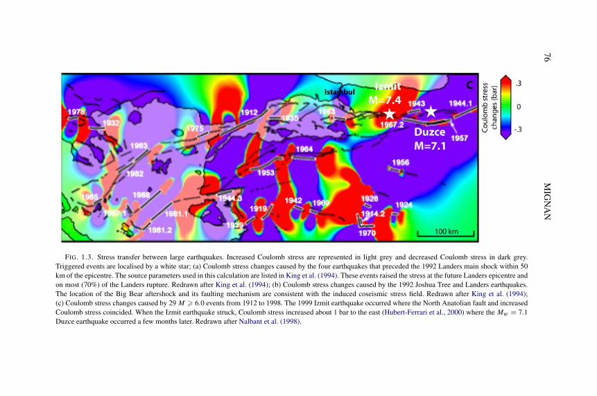
76M
IGN
AN
FIG. 1.3. Stress transfer between large earthquakes. Increased Coulomb stress are represented in light grey and decreased Coulomb stress in dark grey.Triggered events are localised by a white star; (a) Coulomb stress changes caused by the four earthquakes that preceded the 1992 Landers main shock within 50km of the epicentre. The source parameters used in this calculation are listed in King et al. (1994). These events raised the stress at the future Landers epicentre andon most (70%) of the Landers rupture. Redrawn after King et al. (1994); (b) Coulomb stress changes caused by the 1992 Joshua Tree and Landers earthquakes.The location of the Big Bear aftershock and its faulting mechanism are consistent with the induced coseismic stress field. Redrawn after King et al. (1994);(c) Coulomb stress changes caused by 29 M � 6.0 events from 1912 to 1998. The 1999 Izmit earthquake occurred where the North Anatolian fault and increasedCoulomb stress coincided. When the Izmit earthquake struck, Coulomb stress increased about 1 bar to the east (Hubert-Ferrari et al., 2000) where the Mw = 7.1Duzce earthquake occurred a few months later. Redrawn after Nalbant et al. (1998).

THE STRESS ACCUMULATION MODEL 77
FIG. 1.4. Example of stress triggering. Schematic model of Coulomb failure for a fault underconstant loading rate. If an external factor, such as a static stress change �CFS generated by a nearbyearthquake, occurs, the next earthquake on the fault is advanced of �T . Modified from Gomberg etal. (1998).
Modelling studies show that stress redistribution from the Izmit earthquake mayhave led to positive Coulomb stress changes on the fault both to the west, near Is-tanbul (Hubert-Ferrari et al., 2000) and to the east (Barka, 1999). The Mw = 7.1Duzce earthquake that occurred 3 months later, was located in a region of en-hanced stress. It is important to note that this region was in a stress shadow priorto the Izmit earthquake which changed its status. Thus while stress shadows arein general less likely to host future earthquakes, their status can change rapidly ifan event occurs in an adjacent region of high Coulomb stress. Other examples arediscussed by Nalbant et al. (1998).
1.1.5. Temporal Distribution of Large Earthquakes
It is widely held that the time of occurrence of an earthquake on a fault un-dergoing tectonic loading is controlled both by the stress and frictional propertieson that fault and by earthquakes on other faults nearby (Stein, 1999). Figure 1.4shows implications of stress transfer on Coulomb failure models for a fault loadedat a constant background rate (modified from Gomberg et al. (1998)). The failuretime is changed (time shift �T ), independently of the seismic cycle of the fault.
A time shift can be determined from the stress transfer theory in the simpleway indicated in Fig. 1.4. However this assumes that failure depends only ona failure stress level being reached. If stress changes abruptly, transient effectssubstantially modify failure conditions. More complex failure criteria describedas rate-and-state friction have been used to quantify this effect (Dieterich, 1994).

78 MIGNAN
Initially proposed to explain the origin of aftershocks (Section 1.3), rate-and-stateequations summarise in empirical expressions laboratory observations that faultstrength is dependent on slip rate and slip and time history of a fault. Rate-and-state equations have appeal because they allow for a time delay before the onsetof failure and can be applied for the study of stress triggering (e.g. Gomberg etal., 1997, 1998) as well as stress shadows (e.g. Harris and Simpson, 1998). Theyalso describe how some faults may slide stably, whereas others may experience“stick-slip” motion.
Whereas Coulomb friction invokes the simple equation (1.1) to describe thefailure limit, rate-and-state formulations use a more complex relation which alsodescribes the evolution of quantities as they approach failure. Many formulationsof rate and state dependent friction law have been proposed (e.g. Scholz, 1998and references therein). A commonly used form is
(1.2)τ = σ[μ0 + A ln(δ/δ∗) + B ln(θ/θ∗)
]where δ is the sliding speed, θ is a state variable that can be interpreted to representthe effects of contact time between the two surfaces of a fault, and μ0 and A andB are empirically determined coefficients. A − B > 0 leads to stable sliding;B − A > 0 leads to instability (stick–slip behaviour). The asterisked terms arenormalising constants.
In the rate-and-state formalism an earthquake nucleates on a fault when thesliding speed δ “runs away” and increases dramatically above interseismic values(to speeds of the order of centimetres per second). Dieterich (1994) gives the timeof failure in terms of the sliding speed and other variables:
(1.3)t = Aσ
τln
(1 + τ
Hσ δ
)where
(1.4)H = −k
σ+ B
Dc
t is the time to failure, τ is the long-term stressing rate, k is the effective stiffnessfor source nucleation, B is a fault constitutive parameter, and Dc is the character-istic sliding distance.
If an external factor, such as a static stress change generated by a nearby earth-quake, perturbs the sliding speed, it also changes the eventual nucleation time, ortime to failure. Following Dieterich (1994), during the long interval of self-drivenaccelerating slip and before an externally applied stress change, a fault’s slidingspeed depends on the initial stress and state. After a stress step occurs, the slipspeed depends on the new stress and state. Dieterich (1994) explicitly describeshow a stress change perturbs the sliding speed (and, thereby, the time to failure):
(1.5)δ
δ0=(
σ
σ0
)α/A
exp
(τ
Aσ− τ0
Aσ0
)

THE STRESS ACCUMULATION MODEL 79
TABLE 1.1. Comparison between aftershocks and “preshocks” (i.e. accelerating moment release)characteristics
Events Rate change Location Duration
Aftershocks Deceleration Near-field (<fault length) Days–years“Preshocks” (AMR) Acceleration Far-field (<10s fault lengths) Years–10s years
where δ0, τ0, and σ0 are the sliding speed, shear stress, and effective normal stress(which includes pore pressure effects) on the nearby fault before the stress changeand δ, τ , and σ are the sliding speed, shear stress, and effective normal stress (pos-itive for compression) after the stress change; α is a sum of parameters governingnormal stress dependence of the state variables.
1.2. Seismicity Rate Changes
For the purpose of this work, seismicity is separated into different classes ofearthquakes, depending of their occurrence in the seismic cycle of a fault and oftheir spatio-temporal behaviour. These are “preshocks”, foreshocks, mainshocks,aftershocks, and background seismicity. Mainshocks correspond to the largestevents, located on recognisable faults. “Preshocks” and aftershocks are events thatprecede and follow a mainshock, respectively. “Preshocks” (Accelerating Mo-ment Release – AMR) correspond to an increase of the seismicity rate whereasaftershocks correspond to a decay of the seismicity rate (Table 1.1). Foreshockscorrespond to events that occur just before a mainshock, with epicentres closeto the future epicentre of the main event, and they are parts of the nucleationprocess. Background seismicity is composed of random events (constant seismic-ity rate) with possible interactions independent of the seismic cycle on a givenfault, contrary to “preshocks”, foreshocks and aftershocks which are linked to themainshock. Note that other seismicity patterns possibly exist and other definitionscan be proposed but these are not used in the present work.
1.2.1. Aftershocks
Aftershocks are the numerous smaller events that follow a mainshock and area transient response to the abrupt change of stress associated with the main event.Rate-and-state friction provides a popular explanation, but transient effects, due toviscous flow, fault creep, and fluid flow have yet to be fully explored. Other seis-micity is not a transient effect which explains why “preshocks” and foreshocksare less dramatic than aftershocks. A classic preconception is that aftershocksoccur only on the fault that produced the mainshock. Indeed, the earliest af-tershocks sometimes appear to delineate the perimeter of a mainshock rupture,and they are often used to infer the spatial extent of the rupture. As a techni-cal definition, an event counts as an aftershock if it is within one fault length of

80 MIGNAN
the mainshock rupture in any direction, on or off the mainshock fault (Hough,2002). An aftershock sequence continues until the rate of earthquakes in an areareturns to its pre-mainshock levels (background seismicity). The statistical proper-ties of aftershock sequences are associated with three empirical scaling relations:(1) the Gutenberg–Richter frequency-magnitude relation, (2) Bath’s law, and (3)the modified Omori law (see, e.g. Scherbakov et al., 2005, for a review of sta-tistical properties of aftershocks and Kisslinger (1996) for a general review ofaftershocks).
The size-frequency distribution of earthquakes is commonly described in termsof the b-value, the slope of the Gutenberg–Richter relation (Ishimoto and Ida,1939; Gutenberg and Richter, 1956). The empirical relation is given by the equa-tion
(1.6)log N = a − bM
where M is the magnitude, N the cumulative number of earthquakes with mag-nitude > M and a a constant depending on the seismic activity. The b-valuevaries in space and time (e.g. Wiemer and Wyss, 2002) and can range between0.5 and 1.5 (Turcotte, 1992). The most commonly observed b-value for crustalearthquakes is close to unity (Aki and Richards, 1980; King, 1983).
One of the oldest empirical laws of aftershock sequences, known as Bath’slaw, holds that the largest aftershock in a sequence will generally be one mag-nitude unit smaller than the mainshock. Modified versions of Bath’s law havebeen proposed based on an extrapolation of the Gutenberg–Richter statistics (e.g.Scherbakov et al., 2005).
The modified Omori relation is a law of aftershock distributions which de-scribes the decay in aftershock rate with time after a mainshock (Utsu, 1961)(extension of the Omori law (Omori, 1894)). An aftershock sequence will decay,on average, with the reciprocal of time (1/t) as
(1.7)λ0(t) = K(t + c)−p
with K , c and p constants. The p-value is usually near to unity (Fig. 1.5).Aftershocks are best observed after large earthquakes but can also be observed
in background seismicity, which is clustered in both space and time (Zhuang etal., 2005). The Epidemic-Type Aftershock Sequence (ETAS) model suggests thatthe normal occurrence rate of earthquakes in a region results from the triggeringeffect of previous events (e.g. Ogata, 2005; Ogata and Zhuang, 2006). In thisview, all earthquakes are simultaneously mainshocks, aftershocks, and possiblyforeshocks. The ETAS model extends the modified Omori function (Utsu, 1961)to the case where any shock j that occurs at time tj triggers offspring events,so that the seismicity rate at time t is given by the linear superposition of theaftershock effect in the past in such a way that
(1.8)λ(t) = λ0 +∑
j ;tj �t
Kj (t − tj )−p

THE STRESS ACCUMULATION MODEL 81
FIG. 1.5. Aftershocks decay of the 1994 M = 6.7 Northridge earthquake (California) followingthe modified Omori law (dotted curves with p = 0.95, p = 1 and p = 1.05). The best p-valuecorresponds to the standard Omori parameter p = 1. Note that the law is not followed after a certainamount of days due to the limit of the declustering method (see details in Section 2).
where the sum is taken for all shocks j occurring before time t and the coeffi-cient Kj for each shock j contributes to the size of the corresponding offspring,or aftershocks in a wide sense. The constant λ0 (so-called the background seis-mic activity) represents the occurrence rate of events that cannot be explained asthe aftershock effect of past events whose record is available in the data (Ogata,1989). In other words, the ETAS model is fundamentally a “branching” modelwhere each event is triggered by a unique mainshock but each mainshock triggersseveral events depending of its magnitude.
1.2.2. “Preshocks”: Accelerating Moment Release (AMR)
Accelerating moment release or AMR (Fig. 1.6) has been identified for asubstantial number of earthquakes and observed for years to tens of years be-fore a mainshock over tens to hundreds of kilometres from the future epicentre(e.g. Sykes and Jaumé, 1990; Bufe and Varnes, 1993; Knopoff et al., 1996;Bowman et al., 1998; Brehm and Braile, 1998; Jaumé and Sykes, 1999; Robinson,2000; Bowman and King, 2001a; Zoller et al., 2001; Papazachos et al., 2002a;Bowman and Sammis, 2004).

82 MIGNAN
FIG. 1.6. Accelerating moment release (AMR) observed before the 1989, Mw = 7.0, Loma Pri-eta, California, earthquake (figure from Section 2). AMR is best fitted by a power-law curve (Bufe andVarnes, 1993) (dotted curve).
Accelerating moment release is typically modelled by a simple power-law time-to-failure equation (Bufe and Varnes, 1993). This is a relation of the form
(1.9)∑
ε(t) = A + B(tf − t)m
where tf is the time of the large event, B is negative and m is usually about 0.3.A is the value of ε(t) when t = tf . Equation (1.9) is equivalent to the rate-dependent failure equation of Voight (1989) as noted by Sykes and Jaumé (1990)and Bufe and Varnes (1993). The physical relation of this expression to acceler-ating moment release is not verified and other power-laws can fit the pre-eventseismicity rate changes (see Section 3). ε(t) is the cumulative Benioff strain attime t and defined as
(1.10)ε(t) =N(t)∑i=1
√Ei(t)
where Ei is the energy of the ith event and N(t) is the number of events at time t .The cumulative Benioff strain is preferred over the cumulative number of earth-quakes because the multitude of smaller earthquakes would dominate the data,whereas the moderate to large events would dominate if the cumulative seismicenergy alone was used. Therefore the choice of Eq. (1.10) has no physical mean-ing and is only an observational tool.

THE STRESS ACCUMULATION MODEL 83
FIG. 1.7. Coulomb stress changes caused by the 15 March 1979, right-lateral Homestead Valleyearthquake sequence and aftershock distribution. The calculations are carried out in a half-space withthe values of Coulomb stress plotted in the figure being calculated at half the depth to which the faultsextend. The fault, simplified as a single vertical plane, is 5.5 km long and 6 km wide and slip is 0.5 mand it is tapered at the fault ends. Redrawn after King et al. (1994).
1.3. Triggering of Aftershocks by Mainshocks
1.3.1. Spatial Distribution
The stress triggering methods outlined previously (Section 1.1) can be appliedto aftershock distributions. Figure 1.7 shows the spatial distribution of the after-shocks of the 1979 Homestead Valley earthquake in the stress field caused by themainshock. The stress field is composed of four lobes of Coulomb stress rise andfour lobes of Coulomb stress drop. The distributions of aftershocks are consistentwith these patterns (King et al., 1994). Many events are associated with increasesof Coulomb stress of less than 1 bar, while reductions of the same amount appar-ently suppress them. Relatively few events fall in the regions of lowered Coulomb

84 MIGNAN
stress and the clusters of off-fault aftershocks are separated from the fault itselfby a region of diminished activity.
A spatial correspondence between aftershocks and positive Coulomb stress hasbeen documented by a number of researchers (e.g. Karakostas et al., 2003, 2004;Wang and Chen, 2001; Toda and Stein, 2000). Hardebeck et al. (1998) quan-titatively evaluated the role of static stress changes for the apparent triggeringof aftershocks by the 1992 M = 7.3 Landers and 1994 M = 6.7 Northridgeearthquakes (Southern California). For the Landers earthquake, ∼ 85% of eventsbetween 5 and 75 km distance from the mainshock fault plane are consistent withstatic stress change triggering. However it cannot explain the first month of theNorthridge aftershock sequence. Although the aftershocks broadly follow the dis-tribution predicted by stress calculations, some events occur where they are notexpected. Another example is given by Parsons (2002) showing that only about60% of aftershocks are located where the stress increased after a mainshock,meaning that other processes have to be taken into account. Part of such dis-crepancies could be also blamed on the simplification of assuming simple planargeometries of the main faults, from which stress fields are calculated, as well assimplifications of slip distributions. Other studies have been done by Beroza andZoback (1993), Simpson and Reasenberg (1994), Harris et al. (1995), Deng andSykes (1997), Kilb et al. (1997), Toda et al. (1998), Stein (1999). Some studiesalso note that aftershocks sometimes expand in space, probably related to diffu-sion of stresses with time (e.g. Tajima and Kanamori, 1985).
1.3.2. Temporal Distribution
Aftershocks are caused by the change of stress that occurs at the time of themainshock. From rate-and-state equations (Section 1.1.5), Dieterich (1994) ob-tains expressions to quantify the seismicity rate as a function of time after a stressstep (i.e. mainshock)
(1.11)R = rτ /τr
[τ /τr exp(−�τ/(Aσ)) − 1] exp[−t/ta] + 1, τ �= 0
and
(1.12)R = r
exp(−�τ/(Aσ)) + t τr/Aσ, τ = 0
where τr and τ are the stressing rate prior to and following the step, respectively,t is set to zero at the time of the stress step, and
(1.13)ta = Aσ
τ
is the characteristic relaxation time for the perturbation of earthquake rate.It can be noted that Eq. (1.12) has the form of Omori’s law for aftershock decay:
(1.14)R = a
b + t.

THE STRESS ACCUMULATION MODEL 85
Similarly, Eq. (1.11) gives Omori’s law for t/ta < 1, but seismicity rate mergesto the steady state background rate for t/ta > 1. This characteristic of Eq. (1.11)makes it a somewhat preferable representation of aftershock decay for many ap-plications. For further details, see Dieterich (1994).
Rate-and-state friction laws are well accepted and used in many studies con-cerned with the behaviour of aftershocks. Gross and Kisslinger (1997) solved therate-and-state equations for some variables (e.g. for A and σ from Eq. (1.12))by examining the aftershocks of the 1992 Landers earthquake. Gross and Run-dle (1998) have followed a similar tactic and investigated the aftershocks of the1989 Loma Prieta earthquake. Toda et al. (1998) used formulations proposed byDieterich (1994) and investigated the aftershock rates of the 1995 Kobe earth-quake.
1.4. Triggering of “Preshocks” by Loading at Depth: The Stress AccumulationModel
To explain the origin of accelerating moment release observed before largeearthquakes, some studies point out the role of stress loading processes (Bowmanand King, 2001a; King and Bowman, 2003). The concept of “pre-stress field”(Section 1.1.3) permits events which are part of the regional seismicity to be re-lated to a future mainshock. In this section, loading processes are described at thescale of the seismic cycle of one fault or fault segment. Possible stress triggeringfrom a nearby earthquake (Section 1.1) are not taken into account and correspondto independent processes that superimpose their effects on stress loading.
1.4.1. The Seismic Cycle
Fedotov (1968) was perhaps the first to describe a “seismic cycle” or “earth-quake cycle” in the occurrence of smaller earthquakes between great plates ruptur-ing events in the Kurile–Kamchatka region. It is widely accepted that the conceptof a “seismic cycle” is a convenient fiction; reality is more complicated. It doeshowever summarise in a useful way behaviour observed to occur before, duringand after an earthquake. More recent studies describe the evolution of stressesduring the earthquake cycle, in particular for large subduction events, and lookfor the relation to smaller earthquakes (e.g. Dmowska et al., 1988, 1996; Tayloret al., 1996, 1998).
King and Bowman (2003) describe an “earthquake cycle” showing the evolu-tion of the stress field which includes the pre-event, inter-event and post-eventstress fields to simulate seismicity patterns, in particular accelerating moment re-lease. An idealised loading cycle for an infinitely long vertical strike-slip fault isshown in Fig. 1.8. This idealised fault has constant slip along strike. It is localisedand extends through both the crust and upper mantle, which are both assumed to

86 MIGNAN

THE STRESS ACCUMULATION MODEL 87
FIG. 1.8. Schematic illustration of the stress evolution around an infinitely long fault during theearthquake cycle. The system is driven by distant displacement (plate) boundary conditions. Lightgrey colour indicates stresses (shear stress driving fault motion) close to failure. Grey to dark greyindicates lower stresses. Stress values are indicated assuming an earthquake stress drop of about 100bars; (a) Stress condition immediately following the earthquake; (b) At 33% of the earthquake cycle;(c) At 66% of the earthquake cycle; (d) Immediately prior to the next event; (e) Stress conditionsrestored in Fig. 1.8a, but with a further increment of slip. During loading, the stress “hole” (shadow)formed by the last earthquake fills progressively and the stress shadow reduces. From King and Bow-man (2003).
retain long-term strength. King and Bowman (2003) use a purely elastic modelto simulate the evolution of the stress in the earthquake cycle and argue that dis-tributed viscous relaxation in the lower crust or upper mantle is not required atthis time scale by either geological (e.g. Hubert-Ferrari et al., 2003) or geodeticresults (e.g. Meyer et al., 1998).
In the seismogenic zone, the evolution of the stress field is largely controlledby earthquakes. Near the surface, static friction (τs) is greater than dynamicfriction (τd ), resulting in the stick–slip cycling of stress associated with earth-quakes. Beneath the seismogenic zone, static velocity-strengthening occurs (e.g.Tse and Rice, 1986), resulting in stable sliding. The boundary between stick–slip and stable sliding is not abrupt. In the “Schizosphere”, earthquake rupturethat has initiated in a stick–slip zone can propagate into a stable sliding zone(Scholz, 1990b). The system is driven by the displacement boundary conditionsassociated with plate motions, thus subjecting the whole system to the stress nec-essary to drive the fault. At greater depth where plastic flow occurs, the stressrequired to move the fault becomes independent of normal stress. In Fig. 1.8,a light grey colour indicates stress close to that necessary to cause static failureor localised plastic flow. Beneath the seismogenic zone, this remains constant.However, in the seismogenic zone, the stress field drops to the level required tosustain dynamic rupture following an earthquake. Figure 1.8a shows the stressconditions immediately following an earthquake. The amount that the stress leveldrops along the fault is equal to the stress drop in the earthquake, and is shownin dark grey in Fig. 1.8a. As the earthquake cycle progresses, continued stablesliding at depth, as a result of plate loading, steadily restores the region of re-duced stress (Fig. 1.8b–d). At the end of the seismic cycle, the seismogenic zoneagain approaches static failure stress, and a second event occurs (Fig. 1.8e). Fig-ure 1.8 also shows the difference between the absolute stress and the failure stress(for a section perpendicular to the fault) at each step in the loading cycle. Thisis a simplified vision of the earthquake process. However it is adequate for thediscussions which follow that are only concerned with off-fault processes in thefar-field.

88 MIGNAN
1.4.2. Absolute Stress Changes
Unlike conventional Coulomb stress techniques which calculate stress changes,the evolution of the stress field relative to the failure stress is modelled by Kingand Bowman (2003). To examine seismicity through the earthquake cycle, it isnecessary to calculate the stress distribution promoting activity around the mainfault (Fig. 1.9). The stresses are calculated for the cycle of an M = 7.5 event thatrepeats with a stress drop of 100 bars (mean slip of 3 m, fault length of 80 km,downdip extent of 15 km).
In Coulomb stress models, regions of increased stress are shown as havingpositive stresses. The modified stress field presented here accommodates the factthat, as a result of the previous tectonic history, no region ever exceeds the failurestress without an earthquake occurring. Closeness to failure is indicated by a lessnegative stress. This can be considered to be an absolute stress since it is relatedto a specific stress level (failure stress) and is not just the stress change of classicalCoulomb stress calculations.
1.4.3. Tectonic Memory
For real faults, the fault system has been subjected to a tectonic history (leavinga stress memory) that results in an inhomogeneous pre-stress, which must havethe following characteristics: (1) When rupture ceases on the main fault segment,stress at the fault ends and aftershock regions can be brought close to, but notbeyond failure stress. If this were not true, the main fault rupture would continueor main events would occur immediately in the side lobes. (2) When the mainearthquake occurs, the stress on the main fault plane can have reached, but notexceeded the failure stress. If not, the event would have occurred earlier.
To account of these effects, a “tectonic memory stress” must be added. It musthave a form that annuls the positive stresses in the first column of Fig. 1.9. The“tectonic memory” is shown in the centre of Fig. 1.9 and the result of adding it isshown in the second column of Fig. 1.9. Unlike the first column of Fig. 1.9 whichdescribes only stress changes, the second one describes what can be defined as“stress relative to failure stress” (or absolute stress).
1.4.4. Simulation of the Background Seismicity
The stress field shown in Fig. 1.8 and in Fig. 1.9 (the 2 first columns) varysmoothly, but this is not an accurate description of the stress field in the seis-mogenic crust. Since faults are finite in length and active regions are subject tobackground seismicity, some locations must have stresses approaching the failurestress (or background seismicity would not occur), while other areas must havestresses reduced from failure stress by approximately the order of an earthquakestress drop (as a result of previous seismicity).

THE STRESS ACCUMULATION MODEL 89
FIG. 1.9. Stress Accumulation model for a complete earthquake cycle. Stress changes throughthe earthquake cycle, but not the actual stress levels in the system, since at no place can the modelexceed the failure stress without an earthquake occurring. The fault region must have a “memory”of its previous deformation history, represented by the “Tectonic memory stress”. Stress changes arerepresented in column 1, stress relative to the failure stress are represented in column 2 and in column3 where background seismicity is added. See text for details. Modified from King and Bowman (2003).

90 MIGNAN
Figure 1.10 combines the stress evolution through the earthquake cycle ofFig. 1.8 with an irregular stress distribution, that respects the Gutenberg–Richterlaw (see King and Bowman, 2003, for details). The stress drop for the main eventis 100 bars as before, and the amplitude of the stress variations is similar. It be-comes clear from this illustration why pre-event seismicity should appear at adistance from the future epicentre. In Fig. 1.10a, immediately following the bigevent, no peaks in the stress field approach failure in the epicentral region, whichis in agreement with the concept of stress shadow. As stress levels around the pastand future epicentre are reestablished, the peaks first reach failure at a distancefrom the future earthquake (Fig. 1.10b–c). Stress levels near the future epicentreremain too low for any failure. Only immediately prior to the future event arestress levels near to the main fault restored (Fig. 1.10e).
Small events through the cycle can consequently be attributed to the inhomoge-neous stress distribution that must exist in the seismogenic crust as a consequenceof tectonic history. The nature of these inhomogeneities must be such as to createand perpetuate a stress regime that results in the Gutenberg–Richter scaling rela-tions when stress concentrations are relieved by earthquakes (see Fig. 1.10). Bycombining suitable inhomogeneous stress fields with the overall stress evolutiondue to the earthquake cycle (Fig. 1.9, column 3), stress peaks can be identifiedas earthquakes, permitting the creation of artificial catalogues of the location andmagnitude of background seismicity (King and Bowman, 2003).
1.4.5. Simulation of Accelerating Moment Release
The Stress Accumulation model provides a physical explanation for changesin the rate of seismicity observed before the mainshock during a given earth-quake cycle. Figure 1.9 (last column) shows a simulated distribution of seismicitythrough the seismic cycle.
Immediately following a large event, the model produces regions of increasedseismicity (aftershocks) where the overall stress field has been elevated and re-gions of reduced seismicity where the stress field has been reduced (stress shad-ows).
The high stress levels in the aftershock regions decrease due to loading follow-ing the main event. Combined with the stress shadow from the main event, theresult is a broad seismically quiet region of lowered stress around the epicentre.Pre-event seismicity appears as the original stress shadow finally fills as a resultof loading, The increase in seismicity initially occurs several fault lengths awayfrom the main fault and moves inward as the event approaches, forming a “MogiDoughnut” of activity (Mogi, 1969, 1981).
As a result of this effect, the seismic moment release in the region around thefuture epicentre increases as the event approaches. Synthetic catalogues can begenerated that are virtually indistinguishable from real earthquake sequences giv-ing simulated accelerating moment release similar to real patterns (Fig. 1.11).

THE STRESS ACCUMULATION MODEL 91
FIG. 1.10. Changing stress through the earthquake cycle of an infinite length fault for inhomo-geneous stress fields; (a) Immediately after the earthquake, all stress peaks near to the main eventare reduced to below the failure threshold; (b) As the stress hole starts to fill, peaks first reach thethreshold at large distances from the fault; (c) Progressively this preearthquake activity becomes moreintense and approaches the future epicentre; (d) Immediately prior to the next major event, peaks on ornear the main fault plane reach failure. The later modelling shows that this phase occurs very rapidly,explaining why stages shown in b and c are visible for real earthquakes, but the stage in d (classicalforeshocks) is not unequivocally observed; (e) The stress conditions shown in a are restored. Modifiedfrom King and Bowman (2003).

92 MIGNAN
(a) (d)
(b) (e)
(c) (f)
FIG. 1.11. Examples of accelerating moment release observed in real data (a)–(c) and in syntheticcatalogues created from the Stress Accumulation model (d)–(f). Simulated accelerating moment re-lease is similar to real patterns. Redrawn after King and Bowman (2003).
However some aspects of the Stress Accumulation model still need to be con-firmed. Levin et al. (2006) test the “Mogi Doughnut” prediction by examiningseismicity rates as a function of distance before the Landers earthquake but resultscannot conclusively be distinguished from those obtained for a random earthquakecatalogue. The expected spatial distribution of accelerating moment release in re-gions of enhanced stress for real seismicity catalogues is considered in Section 2.

THE STRESS ACCUMULATION MODEL 93
A mathematical formulation for accelerating moment release in the Stress Accu-mulation model to replace the power-law time-to-failure is described in Section 3.
2. SPATIAL DISTRIBUTION OF ACCELERATING MOMENT RELEASE
There are now many studies of accelerating moment release (e.g. Bowmanet al., 1998; Brehm and Braile, 1998; Karakaisis et al., 2002; Papazachos andPapazachos, 2000; Robinson, 2000; Zoller et al., 2001). These all adopt differ-ent geometrical windows in which the effect is identified. These are all centeredaround the epicentre of the event that has already occurred. This approach hasbeen criticised on the grounds that an arbitrary choice of shape can arbitrarily beused to select a region where accelerating seismicity occurs. That it must be cen-tred on the epicentre of the future event has been regarded as a weak constraint.An advance was made by systematically searching for optimum circle size andtime window. A further approach has been to examine random catalogues to de-termine the probability that a given acceleration could occur at random (discussedin Section 4).
A prediction of the Stress Accumulation model is that the events should befound in the regions where stress must accumulate prior to the forthcoming earth-quake and represent a slight unloading of the future fault. Models that invokeaccelerating moment release as a process that adds load to the future earthquakefault predict that the events will not be in these lobes.
In this section the location of the events is examined for earthquakes in Califor-nia and are found to fall in the stress regions predicted by the Stress Accumulationmodel. This result has two important implications. First that the shape of the re-gion is not chosen in an arbitrary way and second, that the Stress AccumulationModel is consistent with observations while other hypotheses are not.
2.1. Introduction
Here an observational test is reported on the origin of accelerating momentrelease, following Mignan et al. (2006b): A progressive increase of seismic acti-vity distributed over a wide region around a future earthquake epicenter is termedAccelerating Moment Release (AMR). This phenomenon has been observed inseveral studies over the last 15 years, although there is no consensus about thephysical origin of the effect. In a recent hypothesis known as the Stress Accumu-lation (SA) model, the AMR is thought to result from the last stage of loading inthe earthquake cycle. In this view, the increasing seismicity is due to minor stressrelease as the whole region becomes sufficiently stressed for the major event tooccur. The stress accumulation model makes specific predictions about the dis-tribution of events in an AMR sequence. Because the AMR is predicted to be a

94 MIGNAN
result of loading on the main fault, the precursory activity should be concentratedin the positive lobes of the far-field stresses calculated by a backslip dislocationmodel of the mainshock. To test this model, AMR is first found in optimal circu-lar regions around the epicenters of each of the Mw � 6.5 earthquakes in centraland southern California since 1950. A backslip dislocation model is then used todetermine which of the precursory events occur in the regions predicted by StressAccumulation. AMR is shown to occur preferentially in the lobes of the backslipstress field predicted by the Stress Accumulation model.
It is generally accepted that large earthquakes strongly perturb the backgroundseismicity rate in large regions. The most obvious of these perturbations areaftershocks, which are generally thought to be triggered by stress transferredfrom the mainshock (e.g. Karakostas et al., 2003, 2004; King et al., 1994;Tod and Stein, 2002a; Wang and Chen, 2001) and may persist for years to decadesafter a great event (e.g. Utsu, 1961). There is also mounting evidence that “stressshadows” from large events can also depress the seismicity rate over broad re-gions (e.g. Harris and Simpson, 1996; Harris, 1998; Harris and Simpson, 2002;Ma et al., 2005; Nalbant et al., 1998; Pollitz et al., 2004; Toda and Stein, 2002b).In contrast, both observational and theoretical studies suggest that seismicity ratechanges before large earthquakes are not as clearly defined. Various workershave documented evidence of both quiescence (e.g. Wiemer and Wyss, 1994;Katsumata and Kasahara, 1999; Ogata, 2005) and activation (e.g. Bufe andVarnes, 1993; Jaumé and Estabrook, 1992; Knopoff et al., 1996) of regional seis-micity before large events.
Although the importance of precursory quiescence was recognised by work-ers as early as Mogi (1969), relatively few studies in recent years have ex-plored this phenomenon (for example, see Holliday et al., 2006; Ogata, 2005;Tiampo and Anghel, 2006). This is primarily due to the difficulty of obtainingstatistically significant results over timescales of months or years. Instead, re-cent work on precursory seismicity rate changes before large earthquakes hasfocused on observations of increased seismic activity over a broad region, knownas “accelerating moment release” (AMR). The earliest studies of accelerating mo-ment release documented seismicity rate changes in the San Francisco Bay region(Bufe and Varnes, 1993; Sykes and Jaumé, 1990). Since then, studies have docu-mented AMR in a variety of regions, including California (Bowman et al., 1998;Bowman and King, 2001a; Knopoff et al., 1996; Sammis et al., 2004), Turkeyand the Aegean (Karakaisis et al., 2002, 2004, Papazachos and Papazachos, 2000;Papazachos et al., 2002a, 2002b, 2002c), New Zealand (Robinson, 2000), thecentral United States (Brehm and Braile, 1998), Alaska (Bufe et al., 1994;Jaumé and Estabrook, 1992), and Sumatra (Jiang and Wu, 2005; Mignan et al.,2006a).
Two broad classes of models have been proposed to explain the origin ofaccelerating moment release before large earthquakes. Several authors havesuggested that AMR is the result of a cascade of small earthquakes progres-

THE STRESS ACCUMULATION MODEL 95
sively building up stress before a large event (e.g. Bowman and Sammis, 2004;Helmstetter et al., 2003; Helmstetter, 2003; Jaumé and Sykes, 1999; Saleur etal., 1996; Sammis and Smith, 1999; Smalley et al., 1985; Sornette et al., 1990;Sornette and Sammis, 1995). In this view, the primary interaction is staticstress transfer, and the accelerating activity is due to the self-organisation of thestress field in a process similar to a phase transition (e.g. Smalley et al., 1985;Sornette et al., 1990). In contrast, King and Bowman (2003) suggested that AMRis a secondary result of the loading of a large fault primarily by aseismic creepon the fault in the lower crust. In their so-called “Stress Accumulation” model,the accelerating activity is associated with a small amount of stress release in avolume of crust surrounding the future earthquake during the progressive loadingof the main fault prior to a major earthquake.
In this paper, we test the model of King and Bowman (2003) using observedseismicity in central and southern California. Because the loading process de-scribed by King and Bowman (2003) produces a spatially heterogeneous stressfield (Fig. 2.1), the AMR predicted by the model should be concentrated in regionsdetermined by the geometry of the eventual mainshock. Therefore, a techniquethat uses the mechanism of the mainshock to constrain the region where accel-erating seismicity is observed (e.g. Bowman and King, 2001a) should providebetter constraints on the observation than a technique that ignores the mechanicsof fault loading (e.g. Bowman et al., 1998). To test this hypothesis, we use theseismicity catalog for central and southern California to search for AMR beforeevents Mw � 6.5 since 1950, similar to the studies of Bowman et al. (1998)and Bowman and King (2001a). Unlike the earlier studies, the seismicity cat-alog is first declustered to minimize spurious results in the pattern recognitionalgorithm. The procedure of Bowman et al. (1998) is then used to find a cir-cular region that optimises the observed AMR. Finally, the backslip model ofBowman and King (2001a) is adopted to discriminate the regions within the cir-cular area where seismicity should be increasing due to loading from below. If theStress Accumulation model of King and Bowman (2003) is correct, then accel-erating seismicity should be found preferentially in the regions identified by thisprocedure. However, if the events causing the AMR are distributed either pref-erentially in the negative lobes or randomly throughout the circular region, thenanother mechanism, such as stress triggering, must play an important role in theorigin of AMR. Although earlier work has addressed this topic qualitatively forselected events (e.g. Sammis et al., 2004), this is the first study that systemati-cally addresses both the importance of correctly identifying the loading regionswhen studying AMR and the relative role of stress triggering versus stress load-ing.
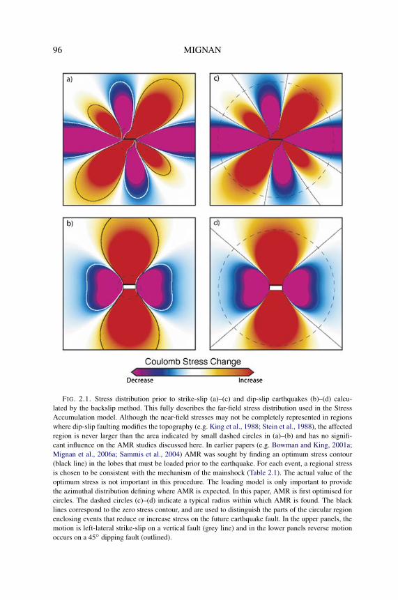
96 MIGNAN
FIG. 2.1. Stress distribution prior to strike-slip (a)–(c) and dip-slip earthquakes (b)–(d) calcu-lated by the backslip method. This fully describes the far-field stress distribution used in the StressAccumulation model. Although the near-field stresses may not be completely represented in regionswhere dip-slip faulting modifies the topography (e.g. King et al., 1988; Stein et al., 1988), the affectedregion is never larger than the area indicated by small dashed circles in (a)–(b) and has no signifi-cant influence on the AMR studies discussed here. In earlier papers (e.g. Bowman and King, 2001a;Mignan et al., 2006a; Sammis et al., 2004) AMR was sought by finding an optimum stress contour(black line) in the lobes that must be loaded prior to the earthquake. For each event, a regional stressis chosen to be consistent with the mechanism of the mainshock (Table 2.1). The actual value of theoptimum stress is not important in this procedure. The loading model is only important to providethe azimuthal distribution defining where AMR is expected. In this paper, AMR is first optimised forcircles. The dashed circles (c)–(d) indicate a typical radius within which AMR is found. The blacklines correspond to the zero stress contour, and are used to distinguish the parts of the circular regionenclosing events that reduce or increase stress on the future earthquake fault. In the upper panels, themotion is left-lateral strike-slip on a vertical fault (grey line) and in the lower panels reverse motionoccurs on a 45◦ dipping fault (outlined).

THE STRESS ACCUMULATION MODEL 97
2.2. Methods
2.2.1. Quantifying AMR
Seismicity rate changes are typically modelled by a simple power-law time-to-failure equation (e.g. Bufe and Varnes, 1993). This is a relation of the form
(2.1)∑
ε(t) = A + B(tf − t)m
where tf is the time of the large event, B is negative and m = 0.3. A is the valueof ε(t) when t = tf . The cumulative Benioff strain at time t is defined as
(2.2)ε(t) =N(t)∑i=1
√Ei(t)
where Ei is the energy of the ith event and N(t) is the number of events at time t .This phenomenon, known as Accelerating Moment Release, has been identifiedfor a substantial number of earthquakes (e.g. Sykes and Jaumé, 1990; Bowmanet al., 1998; Bowman and King, 2001a; Bowman and Sammis, 2004; Jaumé andSykes, 1999; Papazachos et al., 2002a).
We use the algorithms originally developed by Bowman et al. (1998) to identifydomains of accelerating seismicity. In order to quantify the degree of acceleration,Bowman et al. (1998) define a curvature parameter C (c-value), where
(2.3)C = power-law fit RMS error
linear fit RMS error.
Therefore, when the data are best characterised by a power law curve, the parame-ter C will be small. Following the approach of Bowman et al. (1998), the exponentm of Eq. (2.1) is held at 0.3. As a result, when the seismicity is either deceleratingor linearly increasing, C will be at or near unity, whereas accelerating sequenceswill have C < 1.
In this study we use a Levenberg–Marquardt least-squares routine to fit the seis-micity data to Eq. (2.1). Vere-Jones et al. (2001) pointed out that the least-squarestechnique leads to instabilities in the determination of the parameters of Eq. (2.1).However, they also note that the least squares method will produce a “reasonablevisual fit to the data”. In this work, the purpose of Eqs. (2.1) and (2.2) are merelyto provide a logical metric that can be used to identify accelerating activity inthe seismicity data. Because the Stress Accumulation model of King and Bow-man (2003) does not specify the precise functional form of accelerating momentrelease, the power-law time-to-failure is used in this paper both for convenienceand to be consistent with previous works.
2.2.2. Region Optimisation
To detect accelerating moment release in catalog data, it is necessary to isolatethe precursory events in a space/time/magnitude window defined by the model of
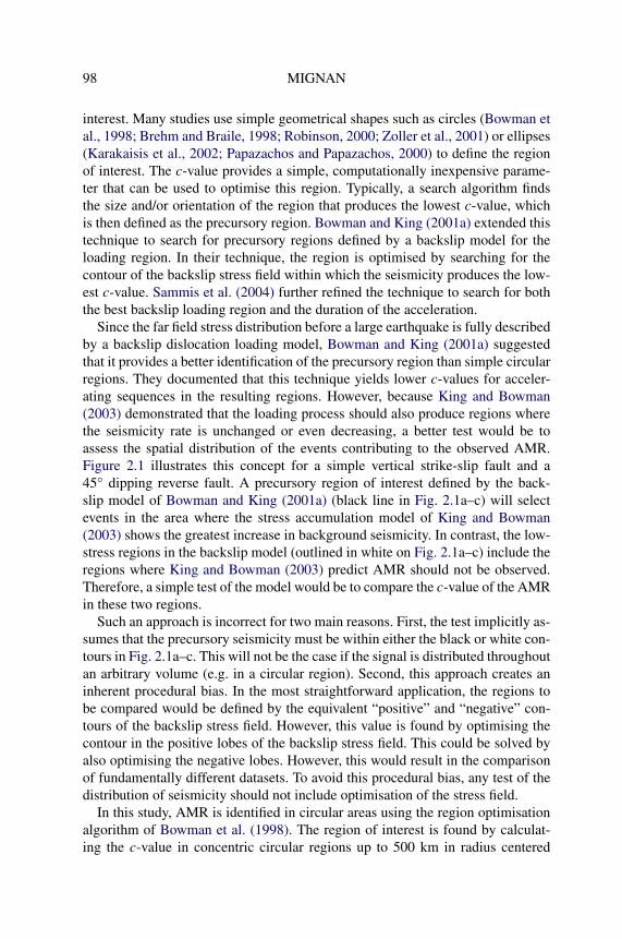
98 MIGNAN
interest. Many studies use simple geometrical shapes such as circles (Bowman etal., 1998; Brehm and Braile, 1998; Robinson, 2000; Zoller et al., 2001) or ellipses(Karakaisis et al., 2002; Papazachos and Papazachos, 2000) to define the regionof interest. The c-value provides a simple, computationally inexpensive parame-ter that can be used to optimise this region. Typically, a search algorithm findsthe size and/or orientation of the region that produces the lowest c-value, whichis then defined as the precursory region. Bowman and King (2001a) extended thistechnique to search for precursory regions defined by a backslip model for theloading region. In their technique, the region is optimised by searching for thecontour of the backslip stress field within which the seismicity produces the low-est c-value. Sammis et al. (2004) further refined the technique to search for boththe best backslip loading region and the duration of the acceleration.
Since the far field stress distribution before a large earthquake is fully describedby a backslip dislocation loading model, Bowman and King (2001a) suggestedthat it provides a better identification of the precursory region than simple circularregions. They documented that this technique yields lower c-values for acceler-ating sequences in the resulting regions. However, because King and Bowman(2003) demonstrated that the loading process should also produce regions wherethe seismicity rate is unchanged or even decreasing, a better test would be toassess the spatial distribution of the events contributing to the observed AMR.Figure 2.1 illustrates this concept for a simple vertical strike-slip fault and a45◦ dipping reverse fault. A precursory region of interest defined by the back-slip model of Bowman and King (2001a) (black line in Fig. 2.1a–c) will selectevents in the area where the stress accumulation model of King and Bowman(2003) shows the greatest increase in background seismicity. In contrast, the low-stress regions in the backslip model (outlined in white on Fig. 2.1a–c) include theregions where King and Bowman (2003) predict AMR should not be observed.Therefore, a simple test of the model would be to compare the c-value of the AMRin these two regions.
Such an approach is incorrect for two main reasons. First, the test implicitly as-sumes that the precursory seismicity must be within either the black or white con-tours in Fig. 2.1a–c. This will not be the case if the signal is distributed throughoutan arbitrary volume (e.g. in a circular region). Second, this approach creates aninherent procedural bias. In the most straightforward application, the regions tobe compared would be defined by the equivalent “positive” and “negative” con-tours of the backslip stress field. However, this value is found by optimising thecontour in the positive lobes of the backslip stress field. This could be solved byalso optimising the negative lobes. However, this would result in the comparisonof fundamentally different datasets. To avoid this procedural bias, any test of thedistribution of seismicity should not include optimisation of the stress field.
In this study, AMR is identified in circular areas using the region optimisationalgorithm of Bowman et al. (1998). The region of interest is found by calculat-ing the c-value in concentric circular regions up to 500 km in radius centered

THE STRESS ACCUMULATION MODEL 99
TABLE 2.1. Characteristics of all earthquakes of m � 6.5 in Central and Southern California between1950 and 2000 and their AMR-search parameters
Earthquake Mainshock source parameters Reg. stress AMR region
Date Mag Strike Dip Length(km)
Width(km)
σ1 σ3 �t
(years)Radius(km)
Kern County 07/21/1952 7.5 60 60 70 15 −30 60 9.75 102Borrego Mountain 04/08/1968 6.5 135 90 30 20 0 90 22.44 23San Fernando 02/09/1971 6.6 125 25 20 15 35 125 14.76 150Coalinga 05/02/1983 6.7 135 15 38 7 45 135 47.84 90Superstition Hills 11/24/1987 6.6 130 90 28 15 −5 85 5.72 136Loma Prieta 10/18/1989 7.0 135 90 17 20 0 90 56.80 200Landers 06/28/1992 7.3 150 90 80 15 15 105 35.05 212Northridge 01/17/1994 6.7 120 35 20 15 30 120 37.45 231Hector Mine 10/14/1999 7.1 145 90 40 15 10 100 47.93 228
on the mainshock epicenter. The duration of the AMR signal is also optimisedas described by Sammis et al. (2004). For each region radius, the beginning ofthe AMR signal is found by calculating the c-value at an array of starting timesranging from the beginning of the catalog (see catalog description below) untilthe year prior to the event. The precursory region is defined as the combinationof region radius and starting time that produces the optimal (lowest) c-value. Af-ter the precursory region is defined, we apply the backslip model of Bowman andKing (2001a) to identify the subset of the circular region that was loaded by slip atdepth (Fig. 2.1b–d). Because the region size under consideration is much greaterthan the thickness of the seismogenic crust, the region optimisation is effectivelya 2-D problem (Bowman and King, 2001a); the Coulomb stress fields used in thisstudy are calculated on optimally oriented planes at a depth of 5 km with a co-efficient of friction of 0.5. The source mechanism used for each event is listed inTable 2.1. With this approach, the identified precursory region is not dependent onany physical model, and event discrimination using the calculated stress field onlyoccurs after optimisation of the AMR. If slip at depth is the primary mechanismdriving the observed AMR, then the c-value for events in the positive pre-stresssub-region should be significantly lower than the c-value in the negative pre-stresssub-region.
2.2.3. Statistical Significance
Given sufficiently flexible search parameters, most optimisation techniques de-signed in this manner will find some degree of acceleration in catalog data. Wehave quantified this bias by using random synthetic seismicity catalogs to deter-mine the likelihood that a seismicity sequence with any given c-value could havearisen stochastically (Bowman et al., 1998). We use a Monte Carlo approach,where 1000 catalogues each composed of 500 events placed randomly in space

100 MIGNAN
FIG. 2.2. Cumulative probability of generating a given C-value by stochastic processes. The figuresuggests that any given synthetic catalog had a 50% chance of generating an optimal C � 0.6, and a25% chance of generating C � 0.5.
and time are created. The events are assigned a uniformly distributed random“longitude” and “latitude” in the range [0 : 1] and a uniformly distributed randomtime in the range [0 : 1]. Each point is indexed to a magnitude that respects theGutenberg–Richter law in the magnitude range [3.5 : 6.0]. Energy for each pointis calculated using the magnitude-energy scaling law (E = 104.8+1.5M ) developedby Kanamori and Anderson (1975). This is then used to generate the cumulativeBenioff strain curve. We test the false-alarm rate in circular regions determined bythe same search algorithm used for the Californian seismicity catalog. For eachsynthetic catalog, the AMR search is done within concentric circles centered onthe point (0.5, 0.5). The c-value is calculated for regions with radii ranging from[0.05 : 0.5] and starting times ranging from [0.0 : 0.90]. AMR cannot be reli-ably observed in regions containing fewer than fifteen events. The optimisationsscheme automatically rejects these regions by assigning them a c-value of 1. Thebest (i.e. minimum) c-value from the search is kept and the process is repeated fora new synthetic catalog.
Figure 2.2 shows the result of this analysis expressed as the cumulative prob-ability of observing a given c-value or higher in the random synthetic catalog.The figure suggests that any given synthetic catalog had a 50% chance of gener-ating an optimal c-value of 0.6 or higher. In contrast, the optimisation procedurefound C � 0.5 in less than 25% of the cases, and C � 0.4 in less than 7% ofthe synthetic catalogs. Because there is a high likelihood of generating C � 0.6

THE STRESS ACCUMULATION MODEL 101
through stochastic processes, any seismicity sequence with C � 0.6 is classifiedin this study as having “unclear” AMR. Lower c-values are more likely to rep-resent AMR driven by nonrandom processes. We also note that these syntheticseismicity tests only produce stable c-values for subregions with more than 25events.
2.3. Data
To facilitate comparison with earlier studies, we will analyse AMR be-fore the 9 M � 6.5 earthquakes in southern and central California stud-ied by (Bowman and King, 2001a) (Table 2.1). The seismicity catalog isprovided by the Advanced National Seismic System (ANSS) (available athttp://quake.geo.berkeley.edu/anss/catalog-search.html). We used events largerthan a magnitude threshold m0 = 3.5 within the time window January 1, 1930 toOctober 16, 1999 (the date of the last M > 6.5 event, Hector Mine). The AMRsearch was limited to a rectangular area 30◦ < latitude < 40◦ and −124◦ <
longitude < −112◦.Unlike previous studies of accelerating moment release, the seismicity catalog
in this study was declustered prior to searching for AMR. Although the precisephysical origin of aftershocks is still poorly understood, most explanations in-voke some form of stress transfer (static and/or dynamic) from a larger event(King and Cocco, 2000; King et al., 1994; Stein, 1999; Toda and Stein, 2000,2002a). Because we are testing a model of seismicity rate changes driven by slipat depth, the unrelated transient effect of aftershocks will contaminate the results.Furthermore, the model of accelerating moment release described by King andBowman (2003) results in a broad, steady increase of activity within the pre-cursory region. Aftershocks to intermediate magnitude events in the precursoryregion represent a burst of activity that may produce anomalous c-values in thesearch algorithm (Fig. 2.3). A detailed description of the declustering techniqueis provided in Appendix.
Changes in the lower magnitude of completeness of the catalog can cause artifi-cial rate changes unrelated to any geologic process. In AMR studies, this generallyis manifested as apparent acceleration through the entire catalog as the sensitivityof seismic networks improves. To evaluate this, the C-value is calculated for the
FIG. 2.3. Influence of the declustering procedure on the calculation of C. (a) A major jump in 1971(San Fernando earthquake and its aftershocks) obscures the background acceleration (C = 0.82).Once major events (m � 6.4, see Appendix 1) and their associated aftershocks are removed, theC-value (C = 0.36) provides a better reflection of changes in the background seismicity rate. (b) Af-tershocks cause a jump in the cumulative Benioff strain curve. The C-value for this sequence is low(C = 0.64), even though the background seismicity is clearly not accelerating. After declustering thesequence gives C = 0.91, more consistent with the linear trend of the background seismicity.

102M
IGN
AN

THE STRESS ACCUMULATION MODEL 103
entire declustered catalog during the time window in which AMR is observed forthe nine earthquakes being studied. In all 9 cases, the evolution of the cumulativeBenioff strain is clearly linear for the entire region (Cmean = 0.96) (see Fig. 2.4and Table 2.2).
2.4. Results and Discussion
For each of the 9 earthquakes studied, it was possible to find clear AMR inoptimised circles centered on their epicenter (Cmean = 0.49, details in Table 2.2).The observed C-values for the circular regions ranged from 0.36 for the 1994Northridge earthquake to 0.64 for the 1968 Borrego Mountain event (Fig. 2.4).Note that the size of the regions found here are slightly different from those foundby previous studies (e.g. Bowman et al., 1998; Zoller et al., 2001). This is becausethe current study used declustered seismicity and the search algorithm jointly op-timised the region size and the duration of the AMR.
The backslip stress models of Bowman and King (2001a) were next used todiscriminate between the “positive” and “negative” pre-stress regions within eachoptimal circular region. Figure 2.5 shows the resulting regions and seismicitycurves for each of the studied events. The dashed lines in Fig. 2.5a representthe 0-bar stress change contour. The areas shaded dark grey are within the opti-mal circular radius and in the positive lobes of the pre-stress field; this is wherethe stress accumulation model of King and Bowman (2003) predicts seismicityleading to AMR should be concentrated. The light grey regions are within theoptimal circular radius but in the negative lobe of the pre-stress field; King andBowman (2003) predict that AMR in this region should be weak or nonexistent.The seismicity curves for the positive and negative pre-stress zones are shown inFigs. 2.5a and 2.5b respectively, and summaries in Table 2.2.
In the positive pre-stress regions, c-values range from C = 0.36 for the 1992Landers earthquake to C = 0.63 for the 1968 Borrego Mountain event, withCmean = 0.49. The seismicity in the positive stress regions produced AMR muchmore reliably than the random synthetic catalogs. Only two events had C > 0.6,Borrego Mountain (C = 0.63) and Kern County (C = 0.61); random catalogshave an approximately 50% chance of producing similar acceleration. Six of theevents (San Fernando, Coalinga, Superstition Hills, Loma Prieta, Landers, and
FIG. 2.4. Results for the AMR-search by circles. The panels on the left show the optimal circularregions for the Kern County, Borrego Mountain, San Fernando, Coalinga, Superstition Hills, LomaPrieta, Landers, Northridge, and Hector Mine earthquakes. The center panels show the cumulativeBenioff strain for the entire region from the beginning of the observed AMR until the time of therespective mainshock. This curve should be linear, indicating that there is no systematic change in thecompleteness of the catalog for the selected magnitude and time windows. The panels on the rightshow the cumulative Benioff strain in the optimal circular region for each event.

104M
IGN
AN

TH
EST
RE
SSA
CC
UM
UL
AT
ION
MO
DE
L105FIG. 2.4. Continued.

106M
IGN
AN
FIG. 2.4. Continued.

THE STRESS ACCUMULATION MODEL 107
TABLE 2.2. C-values for all earthquakes of m � 6.5 in Central and Southern California between1950 and 2000. Values in bold characters correspond to reliable observations of Accelerating MomentRelease (AMR)
Earthquake C
(region)C
(circle)C
(pos. stress)C
(neg. stress)
Kern County 1.00 0.57 0.61 1.00Borrego Mountain 0.94 0.64 0.63 1.00San Fernando 0.93 0.62 0.49 0.93Coalinga 1.00 0.42 0.47 0.63Superstition Hills 1.00 0.45 0.44 1.00Loma Prieta 1.00 0.37 0.40 0.62Landers 1.00 0.47 0.36 0.65Northridge 1.00 0.36 0.47 0.54Hector Mine 1.00 0.47 0.57 0.80MEAN 0.99 0.49 0.49 0.80
Northridge) had C < 0.5; random catalogs have less than 23% chance of pro-ducing any of these individual sequences. The probability of random catalogsproducing all of these sequences is small.
The negative pre-stress region had c-values ranging from 0.54 for the 1994Northridge earthquake to C = 1.0 for the 1952 Kern County, 1967 BorregoMountain, and 1987 Superstition Hills events, with Cmean = 0.80. Only one eventhad C < 0.6 (Northridge).
We note that the circular search by itself appears to outperform the model ofBowman and King (2001a). Furthermore, the regions found here are significantlydifferent from those observed in earlier works (e.g. Bowman et al., 1998; Bowmanand King, 2001a). However, a direct comparison between earlier works and theresults of this paper is not possible for two main reasons. First, Bowman and King(2001a) performed an optimisation of the stress contour used to define the regionof interest, whereas no optimisation of the stress field was permitted here. Second,Bowman and King (2001a) did not decluster the seismicity, unlike the data used inthis study. Therefore, the results of this study should not be interpreted to indicatethat circular regions outperform the backslip loading model.
What do these results suggest about the physical mechanism driving observedaccelerating moment release before large earthquakes? If cascading interactions
FIG. 2.5. Results for the AMR-search by regions of positive and negative pre-stress. The panelson the left show the search regions. The optimal circular region (of Fig. 2.4) is shown. The dashed lineindicated the 0-bar stress change contour; regions of positive stress are shaded dark grey and regionsof negative stress are shaded light grey. The orientation of the regional stress field used to calculatethe pre-stress is indicated by the arrows on the map. The central panels show the cumulative Benioffstrain in the positive stress regions. The panels on the right show the cumulative Benioff strain in thenegative stress regions. See text for discussion.
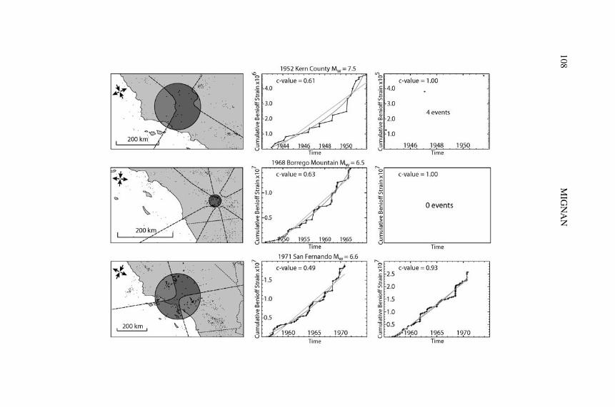
108M
IGN
AN

TH
EST
RE
SSA
CC
UM
UL
AT
ION
MO
DE
L109FIG. 2.5. Continued.

110M
IGN
AN
FIG. 2.5. Continued.

THE STRESS ACCUMULATION MODEL 111
driven by stress transfer from smaller events is the driving mechanism of AMR,then the precursory rate changes should be expected to be strongest in the nega-tive lobes of the Coulomb pre-stress field. In contrast, if the stress accumulationmodel of King and Bowman (2003) is correct, then AMR should be more apparent(smaller c-values) in the positive lobe of the pre-stress field. The latter predictionis true for all 9 earthquakes in the study region, consistent with the predictionsof King and Bowman (2003). This suggests that slip at depth has a strong, if notdominant, influence on the development of accelerating moment release. Whilethis alone does not rule out cascading seismicity as an important factor in the evo-lution of regional seismicity, it does suggest that static stress triggering does notplay an important role in the generation of accelerating moment release.
The relative importance of stress triggering and (stress) loading in generatingprecursory AMR has implications not only for the spatial distribution of acceler-ating seismicity in the region of an impending earthquake, but also for the sizeof events that might be expected to exhibit precursory AMR. Simple static stressinteraction models (Fig. 2.6) demonstrate the relative role of stress triggering andstress loading for events with different ratios of fault length, L, to width, W . Fig-ure 2.6 shows the fault plane viewed face-on, with a dotted rectangle indicatingthe site of an upcoming event. The grey region at the base of each figure repre-sents the fault in the lower crust, which moves aseismically to load the overlyingseismogenic portion of the fault. The white rectangles represent the rupture areaof earlier events along strike with sizes comparable to the impending earthquake;the colouring represents the static stress change in the seismogenic zone fromboth the earlier adjacent events and creep on the fault in the lower crust.
For events with L/W ∼ 1 (Fig. 2.6a), stress transfer from adjacent events con-tributes more to the overall stress on the fault than the loading caused by aseismiccreep in the lower crust. This can be seen by comparing the 10-bar stress contourfor adjacent event (solid line) and the loading from below (dashed line). In con-trast, the stress field on the fault plane of events with L/W > 1 (Fig. 2.6b) isdominated by aseismic creep on the fault in the lower crust. Although static stresstriggering certainly increases the stress on the plane of the impending earthquake,the effect is restricted to only a small section of the fault. Comparing the 10-barstress contour for both the adjacent event and loading from below suggests thatlarge earthquakes are dominantly loaded by aseismic slip on the fault at depthrather than stress transfer from nearby earthquakes, consistent with the resultspresented here.
Because stress triggering is the dominant loading mechanism for small and in-termediate (L/W ∼ 1) events, slip at depth will not necessarily be the dominantloading mechanism on the rupture plane of the small earthquakes. Unlike largeevents, it is likely that any precursory seismicity before small earthquakes is dom-inated by traditional stress transfer. However, any systematic test of this conceptfor small events would require much higher precision catalog locations than areroutinely available at present. Furthermore, the stress-based approach used in this

112 MIGNAN
FIG. 2.6. Role of stress triggering and stress loading for faults of different L/W ratios. The colour-ing indicates the stress level. In the models, a surface that has already ruptured (white rectangle)increases stress around it. Under the seismogenic zone, the fault (shaded grey) moves aseismicallycausing loading. The relative contribution of each effect can be assessed by looking at the 10 bar con-tour indicated for each separately. (a) For small events, L/W ∼ 1, the stress field on the fault planemay be weakly influenced by loading and greatly influenced by adjacent events; (b) For a large event(L/W > 1), loading predominates the stress field on the fault plane of the future event.
work is not practical for small earthquakes since the focal mechanisms for theseevents are not well constrained in most earthquake catalogs. As a result, investi-gations of precursory activity for small-to-intermediate magnitude seismicity aremore suitable using statistical techniques such as the Pattern Informatics method(e.g. Tiampo et al., 2006).
This simple model for the relative importance of stress triggering versus faultloading also suggests that the approach of Bowman et al. (1998) can only bereliably used to observe AMR before large earthquakes. Furthermore, our resultssuggest that models of regional seismicity that are driven primarily by stress trans-fer and fail to account for loading by aseismic creep at depth (e.g. Robinson etal., 2005) will not produce systematic accelerating moment release before modelevents. Because the loading mechanism for events with L/W > 1 is dominated byaseismic creep on the fault in the lower crust, seismicity rate changes before large

THE STRESS ACCUMULATION MODEL 113
earthquakes are more accurately represented by the model of King and Bowman(2003), as supported by the results of this study.
2.5. Appendix
Declustering Algorithm: Aftershocks represent a local perturbation of the back-ground seismicity rate as the stress field is reorganised following an earthquake.This process is independent of the slow regional seismicity rate change rep-resented by AMR. However, large aftershock sequences produce step-functionchanges in the regional seismicity rate. This is evident in the cumulative Benioffstrain plot for the entire California catalog shown in Fig. 2.A1a. The c-valueanalysis described in the main text could incorrectly identify these aftershockclusters as AMR. To alleviate this problem, the seismicity catalog in this study isdeclustered before the c-value analysis is run.
The average seismicity rate is defined here as the number of events M � 3.5in a two-week window. For the duration of the catalog (Fig. 2.A1), the averageseismicity rate defined in this way is 17 events per two weeks. We classify anevent as part of an aftershock cluster if it:
(1) occurs when the seismicity rate is greater than the long-term average;(2) is preceded by an event greater than some arbitrary mainshock threshold,
Mmain;(3) is within some distance, Rcluster, of a mainshock.
For this study, Rcluster = 50 km. The mainshock threshold, Mmain, is a parameterthat is adjusted to achieve the desired level of declustering for the catalog. Forinstance, the dashed lines in Fig. 2.A1b indicate the occurrence of M � 6.4events in the catalog used here. By inspection, it is clear that most of the burstsin seismicity rate coincide with events M � 6.4. We therefore select Mmain =6.4 as the mainshock threshold for the declustering. The declustering algorithmworks by deleting all aftershocks until the seismicity rate is equal to the long-termaverage.
The results of this declustering algorithm are shown in Fig. 2.A2. In the newcatalogue, 4069 events have been removed (28 of m � 6.4) for a total of 31 415events. Figure 2.A2a shows the mapped distribution of “independent” earthquakes(black dots) and deleted aftershocks (white diamonds). Figure 2.A2b shows theseismicity rate of the declustered catalog. Note that not all of the clusters wereremoved. Our goal is not to identify all aftershocks, but to minimize their impacton the cumulative seismicity curves. An inspection of Fig. 2.A2c shows that thisis the case; the steps in the curve caused by aftershocks have been removed, re-sulting in a smooth seismicity curve for the entire catalog. The same effect can beachieved with a wide range of declustering parameters.

114 MIGNAN
FIG. 2.A1. Seismicity catalogue for Central and Southern California (from 1930 to 2005) beforedeclustering. (a) Evolution of the cumulative Benioff strain for the entire catalog. Note the irregularityof the curve, corresponding to the presence of large events and their associated aftershocks. (b) Seis-micity rate through the duration of the catalog. The averaged number of events (n ∼ 17) correspondsto the background seismicity for a period of 2 weeks (average background rate). The majority of thepeaks in the seismicity rate can be related to the occurrence of M � 6.4 earthquakes.

THE STRESS ACCUMULATION MODEL 115
FIG. 2.A2. Declustered seismicity catalog. (a) Map of the region. White diamonds correspondto events that have been removed by the declustering procedure (see text for details). Each cluster iscomposed of a large event (m � 6.4) and its aftershocks. (b) Seismicity rate of the declustered catalog.Some high seismicity rate peaks are still present. These clusters are either swarms or are preceded aM < 6.4 mainshock, and are left in the catalog. (c) Evolution of the cumulative Benioff strain in theentire declustered catalog. Note the relatively linear trend of the curve after declustering.
2.6. Supplemental Information
Validity of the declustering method: If the methodology is correct, events re-moved from the catalogue should be aftershocks of large earthquakes. The modi-fied Omori relation describes the decay in aftershock rate with time after a main-shock (Utsu, 1961) (extension of the Omori law (Omori, 1894)). An aftershocksequence will decay, on average, with the reciprocal of time (1/t) as following:
(2.4)λ0(t) = K(t + c)−p
with K , c and p constants. The p-value is usually near the unity.

116 MIGNAN
FIG. 2.A2. Continued.

TH
EST
RE
SSA
CC
UM
UL
AT
ION
MO
DE
L117

118 MIGNAN
FIG. 2.7. Validation of the declustering method by verification of the Omori law for clusters oflarge earthquakes M � 6.5 in Central and Southern California between 1950 and 2000. Curves cor-respond to the modified Omori law with three different p-values, p = 0.95, p = 1.00, p = 1.05 (upto down). The Omori decay model was fit by trial and error to best match the data; (a) Kern Countyearthquake; (b) Borrego Mountain earthquake; (c) San Fernando earthquake; (d) Coalinga earthquake;(e) Superstition Hills earthquake; (f) Loma Prieta earthquake; (g) Landers earthquake; (h) Northridgeearthquake; (i) Hector Mine earthquake.
The Omori decay model was fit by trial and error to best match the data. It hasbeen verified for all earthquakes of M � 6.5 in Central and Southern Califor-nia from 1950 to 2000, corresponding to events used for the study of AMR. Forthe 9 earthquakes, the corresponding cluster follows a decay, which can be rep-resented by the modified Omori with p-values between 0.95 and 1.05 (Fig. 2.7).This confirms that the clusters are composed of aftershocks.
The declustering procedure adopted does not remove all aftershocks associ-ated with events of magnitude larger to Mc but it removes a sufficient number toprevent the cluster from disturbing the stability of the calculation of the c-value.
3. TEMPORAL DISTRIBUTION OF ACCELERATING MOMENT RELEASE
“[. . . ] a self-organised critical state is charactered by power law distributions of eventsizes and long-range spatial correlation of fluctuations around the stationary state.Because earthquakes are characterised by several power laws, such as the Gutenberg–Richter frequency-magnitude relation, Omori’s Law for aftershocks, and the fractaldistribution of hypocenters, the application of this concept of self-organised criticalityto earthquakes is now often taken for granted in the seismological community.”
C.G. Sammis and D. Sornette, Positive Feedback, memory, and the predictabil-ity of earthquakes, Colloquium Proc. Natl. Acad. Sci. USA (2002)
A number of complex natural phenomena (i.e. non-linear dynamic systems)exhibit power-law frequency-size statistics in a very robust manner. This hasbeen observed from Physics to Biology, from Languages to Economics. It is alsoobserved in natural hazards, such as earthquake populations, forest fires and land-slides (e.g. Turcotte et al., 2002).
It is commonly thought that power-law distributions are a “signature” of self-organised criticality systems (Bak et al., 1987). In that state, small perturbationsresult in chain reactions (avalanches), which can affect any number of elementswithin the system. Proponents of the theory see multiple manifestations of self-organised criticality in earthquake populations, from the Gutenberg–Richter lawto accelerating moment release. In their view, accelerating moment release repre-sents a cascade of events that leads to the largest one. This concept is not the same

THE STRESS ACCUMULATION MODEL 119
as the Stress Accumulation model described in Sections 1 and 2 where accelerat-ing moment release only represents the “signature” of the final step of aseismicloading on the major fault that is going to rupture (Elastic Rebound theory).
There has been a wide interest in comparing earthquake populations to criticalsystems as it can be seen in many reviews or special issues concerned with earth-quake interactions and accelerating moment release (e.g. Jaumé and Sykes, 1999;Sammis and Sornette, 2002; Papazachos, 2003; Tiampo and Anghel, 2006). How-ever this apparent consensus can lead to misunderstanding and the application ofcriticality to earthquake populations should not be taken for granted. For example,the Stress Accumulation model is understood by Tiampo and Anghel (2006) as amethod based on the concept of stress transfer, but with a critical point physicalorigin. This is not correct. Sammis and Sornette (2002) also associate the StressAccumulation model with a finite-time singularity process based on the conceptof critical point, but this is not a necessary condition.
Since the Stress Accumulation model, which does not draw on the concept ofcriticality has been proposed as an explanation for accelerating moment release,the role of critical processes becomes questionable. However, it can be difficult toargue for or against criticality concepts since, by definition, these processes canonly be caught by looking at the system globally (e.g. Self-Organised Criticalitysystems (Bak et al., 1987, 1988)) making it difficult to verify the reality of suchunderlying processes. It may be more useful to ask if such approaches have anypractical utility.
The purpose of this chapter is to show that accelerating moment release canbe formulated in terms of stress transfer with no need of criticality. First, criticalprocesses are reviewed and the power-law time-to-failure equation explained inthese terms (Section 3.1). Then a new mathematical formulation is demonstratedbased on the Stress Accumulation model that draws on none of these concepts(Section 3.2).
3.1. Origin of Accelerating Moment Release from Critical Processes
3.1.1. Power-Laws: “Signature” for Criticality?
Self-organised criticality: The sandpile model (Bak et al., 1987, 1988; Bak andTang, 1989; Bak and Paczuski, 1995) was first proposed to explain the concept ofSelf-Organised Criticality and is defined as follows.
The height (i.e. slope in real cases) of the “pile” at the point (i, j) of a grid isdenoted Z(i, j). Each height corresponds to an integer value (counter). At eachtime step, the height at some random point is increased by 1 unit, Z(i, j) →Z(i, j) + 1. If the height at that site now exceeds an arbitrary critical height Zcr,then a toppling event occurs, where the height of the unstable site is reduced by4 units and the height at each of the four neighbours on the grid is increased by 1

120 MIGNAN
FIG. 3.1. Sandpile model; (a) Domain (areal extent) for several different avalanches in a sandpilemodel (SOC). Each avalanche (light grey colour) was triggered by the addition of a single increment(at a random point of the grid). The various shadings indicate heights 0–4, with 4 being the criticalheight. The light grey colour indicates sites that have toppled. White sites are active, toppling sites;(b) Scaling-law obtained by a sand pile model following (Bak et al., 1987) (see algorithm in Appen-dix A). Log–log plot of the frequency of occurrence of given avalanche size D(s) versus the size ofthe avalanche s.
unit. ⎧⎨⎩
Z(i, j) → Z(i, j) − 4,
Z(i ± 1, j) → Z(i ± 1, j) + 1,
Z(i, j ± 1) → Z(i, j ± 1) + 1.
This is true except along the boundaries where “sand” is thrown out of the “pile”.If any of the neighbouring sites are now unstable (Z > Zcr), the process continuesuntil none of the Z values in the grid exceeds the critical value. Then an avalancheis over, and a new avalanche can be started by adding another increment to thegrid.
One can imagine that for each point in the grid, there is a domain D which is theset of all points whose Z value was changed as a result of the initial perturbation.Figure 3.1a plots D for several different single perturbations that resulted in anavalanche. Each domain D has a finite size s, which is the areal extent of an

THE STRESS ACCUMULATION MODEL 121
FIG. 3.1. Continued.
avalanche (number of topplings). Figure 3.1b plots D as a function of s. The figureclearly shows a power-law distribution, implying the system has self-organised toa critical state. The relation is
(3.1)log D(s) ∝ s
where D(s) is the frequency of occurrence of avalanches of size s. Each domain D
(i.e. avalanche) was triggered by the addition of a single perturbation at a randompoint of the system. Note that avalanches also exhibit a power law distributionthrough time (Bak et al., 1987). Other models than the sandpile model have alsobeen proposed, such as forest fire models (e.g. Turcotte et al., 2002; Papazachos,2003) and slider blocks models (e.g. Carlson and Langer, 1989).
Critical point theory: In general, self-organised criticality formulations sufferfrom the problem that there should be no upper limit to the size of the largestevent and they also generally fail to address the observations that major earth-quakes recur on major recognisable faults. This can be resolved if it is explainedas a finite-size effect (e.g. Sammis and Smith, 1999). In the critical point view,a large earthquake plays a special role and signals the end of a cycle on its faultnetwork (see, e.g. Sornette and Helmstetter, 2002).
Singularities such as phase transitions characterise critical phenomena and crit-ical points. The simplest representative dynamic evolution equation leading to a

122 MIGNAN
finite-time singularity is
(3.2)dE
dt= Em, with m > 1.
Its solution is
(3.3)E(t) = E(0)
(tc − t
tc
)−1/(m−1)
where the critical time tc = (m−1)/[E(0)]m−1 is determined by the initial condi-tion E(0). This kind of equation can be used for example in crack growth models,damage models or percolation models (see Sammis and Sornette, 2002, for moredetails).
3.1.2. Accelerating Moment Release as a Critical Phenomenon
In a self-organised criticality system, accelerating moment release is thoughtto be the consequence of the growth of the spatial correlation length. A smallrupture can only grow into a large earthquake if a critical value of the spatialcorrelation length of the stress is reached. In the preparatory process before amainshock, long-range correlations are established by the redistribution of stressfrom smaller to larger scales. In other words, small events cascade into larger onesto finally lead to the largest one (mainshock).
Some studies explain the accelerating moment release power-law using cascadetriggering (e.g. Sornette and Helmstetter, 2002) or change of scaling in hierarchi-cal models (e.g. Sornette and Sammis, 1995; Saleur et al., 1996). Other studiesexplain the origin of accelerating moment release using rock fracture mechan-ics, such as fiber-bundle models (e.g. Turcotte et al., 2003) or continuum damagemodels (e.g. Ben-Zion and Lyakhovsky, 2002).
Following existing theories and models based on self-organised criticality,an important number of studies that search for accelerating moment release inseismicity catalogues assume that these seismicity patterns are due to criticalprocesses (e.g. Bowman et al., 1998; Zoller et al., 2001; Papazachos et al., 2002a).Some other studies test the critical point hypothesis by searching for indicators inearthquake populations, such as the growth of the spatial correlation length (Zollerand Hainzl, 2002) or seismic quiescence (Hainzl et al., 2000).
3.1.3. Previous Formulations of Accelerating Moment Release
Epidemic-Type Aftershock Sequence model: Sornette and Helmstetter (2002)show that for certain conditions, the rate of seismic activity in the Epidemic-TypeAftershock Sequence model diverges in finite time according to
(3.4)N(t) ∝ 1/(tc − t)m

THE STRESS ACCUMULATION MODEL 123
where N(t) is the seismicity rate. These specific conditions are obtained whenthe system is “supercritical” (as opposed to subcritical) (Helmstetter and Sornette,2002). In that case, the average rate of seismicity N(t) is no longer linear due tothe role of large earthquakes. The nonlinearity is expressed as a positive feedbackand self-amplifies leading to the finite-time singularity of Eq. (3.4).
This can be verified by stacking ETAS-derived synthetic catalogues to estimatethe probability of events before “mainshocks”. By relaxing the requirement thataftershocks are smaller than mainshocks, “foreshocks” can be produced. Becauseof the Omori decay (proportional to 1/t), “foreshocks” are more likely to occurimmediately before an event in a ETAS system. In other words, foreshock statis-tics and aftershock statistics are symmetric about the time of the mainshock, theonly differences are that aftershocks have a much higher a-value than foreshocksand that foreshocks follow a power-law acceleration (i.e. accelerating moment re-lease) whereas aftershocks follow a power-law deceleration. For more details, seeSornette and Helmstetter (2002), Helmstetter and Sornette (2002), Helmstetter etal. (2003), Helmstetter (2003).
Hierarchical models and Renormalisation Group Theory: Sornette and Sammis(1995) and Saleur et al. (1996) proposed that accelerating moment release can beformulated using the Renormalisation Group Theory, viewing accelerating mo-ment release as a critical phenomenon in a hierarchical fault system. This theoryis the transformation of a set of equations from one scale to another, by chang-ing of variables. Sornette and Sammis (1995) postulated a one-parameter (time tofailure) discrete renormalisation group, expressing how the (cumulative) seismicrelease ε at given time t can be related to that at another time t ′. The times t andt ′ have a relation of the form x′ = φ(x) where x = tc − t , tc is the failure time,and φ is called the renormalisation group flow map. Then
(3.5)f (x) = g(x) + 1
μf(φ(x)
)where f (x) = ε and μ is a scaling constant. g(x) represents the nonsingularpart of the function f (x) (see Saleur et al., 1996, for details). Saleur et al. (1996)show that the critical point x∗ is the time at which f (x) becomes singular andthat a necessary condition is φ(x∗) = x∗. Using the conditions φ(0) = 0 andφ(x) = λx + · · · (linearised transformation), the solution of Eq. (3.5) close tox = 0 is f (x) ∼ xm with m = log μ/ log λ. Equation (1.9) can be derived fromthis last equation.
Sornette and Sammis (1995) add an imaginary part to the exponent m and find
(3.6)ε(t) = A + B(tf − t)m[
1 + C cos
(2π
log (tf − t)
log λ+ φ
)]with the term added to Eq. (1.9) being the logarithm periodic correction for thechange of scale associated with the incoming mainshock. Several other studies

124 MIGNAN
FIG. 3.2. Schematic illustration of the failure of a fiber-bundle with uniform load sharing; (a) Eachof the fibers carries one-quarter of the load F0; (b) One fiber has failed and each remaining fiber carriesone-third of the load F0; (c) Two fibers have failed and each remaining fiber carries one-half of theload F0; (d) All four fibers have failed and no load is carried. Redrawn after Turcotte et al. (2003).
associate hierarchical models of faults with the Renormalisation Group Theory toidentify accelerating moment release (e.g. Huang et al., 1998). However Eq. (3.6)has not proved to be a more accurate predictor of accelerating moment releasethan Eq. (1.9) (Gross and Rundle, 1998).
Fiber-bundle models: An approach to brittle failure is the fiber-bundle model(e.g. Newman and Phoenix, 2001) which takes into account a composite materialmade up of strong fiber embedded in a relatively weak matrix. The failure statis-tics of the individual fibers that make up the fiber-bundle are specified and canbe either static or dynamic. In general, experiments favour dynamic-failure fiber-bundle models (Turcotte et al., 2003). When stress is applied to a fiber-bundle, thefibers begin to fail. The fiber-bundle model can also be used as a simple modelfor friction where the fibers represent the asperities on a surface and thus can beapplied to fault rupture.
The failure of a simple fiber-bundle under uniform load sharing is illustrated inFig. 3.2. Initially the load on the bundle F0 is carried equally by the four fiberswith F = 1
4F0. The weakest fiber fails and the load on that fiber is now carriedby the surviving fibers with F = 1
3F0. The stress on each fiber increases from theoriginal value σ0 to 4
3σ0. The process of failure followed by stress redistributioncontinues until all fibers fail and no load can be carried.
As fibers fail, the stress on the remaining fibers increases leading to acatastrophic failure of the bundle and are equivalent to the microcracks that occurin a uniform brittle material as it is stressed to failure. A characteristic of materialfailure are the emergence of acoustic emission events, generated by microcracks

THE STRESS ACCUMULATION MODEL 125
(Scholz, 1998). The microscopic fiber-bundle model can be used to obtain the pre-dicted rate of the acoustic emission events which is a power-law time-to-failureequation (Turcotte et al., 2003). First it is necessary to prescribe the dependence ofthe hazard rate ν on the stress σ . For engineering materials it is standard practice(Newman and Phoenix, 2001) to empirically assume the power-law relation
(3.7)ν(t) = ν0
[σ(t)
σ0
]ρ
where ν0 is the hazard rate corresponding to the initial fiber stress σ0 (values of ρ
found experimentally in a range 2 to 5).Equation (3.8) is the rate at which energy is radiated in acoustic emission events
during the failure of a fiber-bundle
(3.8)dea(t)
dt= ηaν0σ
20
2E0
1
(1 − t/tf )(ρ+1)/ρ
where ea is the energy associated with the acoustic emission event, ηa the acousticemission efficiency (i.e. fraction of lost energy), ν0 the hazard rate correspondingto the initial fiber stress σ0, E0 the Young’s modulus of fibers and tf the failuretime. Details of the demonstration can be found in Turcotte et al. (2003).
By analogy between the energy associated with the acoustic emission event andthe seismic energy release by a seismic event, Turcotte et al. (2003) find
(3.9)εB(t) = εBf − σ0(ρ − 1)
2ρ
√ηaν0
2E0
(1 − t
tf
)(ρ−1)/(2ρ)
where εB is the cumulative Benioff strain and εBf the Benioff strain when thelarge earthquake occurs. Equation (3.9) is used in some AMR studies (Ben-Zionand Lyakhovsky, 2002; Turcotte et al., 2003).
Continuum damage models: The anelastic deformation of solids is often treatedusing continuum damage mechanics. Turcotte et al. (2003) show that continuumdamage models can give exactly the same solution for material failure as the fiber-bundle model. The power-law scaling obtained by both models is consistent withthe power-law seismic activity observed prior to some earthquakes.
In linear elasticity, σ = E0ε where E0 is the Young’s modulus of the undam-aged material, a constant. Once microcracking is occurring, there is a deviationfrom linear elasticity. These microcracks weaken the material and for a givenstress σ , the strain ε is greater than the value predicted by linear elasticity. The re-lation becomes σ = Eeffε where Eeff is the effective Young’s modulus, no longerassumed to be a constant. A continuum approach to this process is to introduce adamage variable α (e.g. Ben-Zion and Lyakhovsky, 2002) so that
(3.10)Eeff = E0(1 − α).

126 MIGNAN
The damage variable α quantifies the deviation from linear elasticity. In general0 � α � 1. With α = 0, linear elasticity is obtained but when α = 1, failureoccurs.
Using the relation (see details in Lyakhovsky et al., 1997)
(3.11)dα
dt= Cε2
(Ben-Zion and Lyakhovsky, 2002) integrate Eq. (3.10), which gives
(3.12)α = 1 − [1 − (
3Cσ 2/E20
)t]1/3
.
Substituting Eq. (3.12) back into Eq. (3.10) leads to strain accumulation in thepower law form
(3.13)ε = σ/E0[1 − (
3Cσ 2/E20
)t]−1/3
.
Using tf = E20/3Cσ 2 in Eq. (3.13), defined by setting α = 1 in Eq. (3.12), and
changing constants gives
(3.14)ε(t) = σ/E0(�t/tf )−1/3
with �t = tf − t . Finally, Ben-Zion and Lyakhovsky (2002) obtain for the cumu-lative Benioff strain the form
(3.15)∑
M1/20 (t) = A1 + A2t + A3(�t/t)1/3.
Equation (3.15) is equivalent to Eq. (1.9) with m = 1/3 with the backgroundseismicity taken into account (i.e. the linear part of the equation).
3.2. Origin of Accelerating Moment Release from Stress Loading
The previous formulations of accelerating moment release have all been pro-posed based on the idea that accelerating moment release corresponds to somecascade triggering leading to the mainshock. However, another formulation basedon the Stress Accumulation model can be proposed where accelerating momentrelease is formed by a different process.
3.2.1. Introduction
Here a new mathematical formulation of accelerating moment release basedon the Stress Accumulation Model is reported, following Mignan et al. (2007):Large earthquakes can be preceded by a period of accelerating seismic activity ofmoderate-sized earthquakes. This phenomenon, usually termed accelerating mo-ment release, has yet to be clearly understood. A new mathematical formulationof accelerating moment release is obtained from simple stress transfer consider-ations, following the recently proposed Stress Accumulation model. This model,

THE STRESS ACCUMULATION MODEL 127
based on the concept of elastic rebound, simulates accelerating seismicity fromtheoretical stress changes during an idealised seismic cycle. In this view, acceler-ating moment release is simply the consequence of the decrease, due to loading,of the size of a stress shadow due to a previous earthquake. We show that a power-law time-to-failure equation can be expressed as a function of the loading rate onthe fault that is going to rupture. We also show that the m-value which is thepower-law exponent can be defined as m = D/3 with D a parameter that takesinto account the geometrical shape of the stress lobes and the distribution of ac-tive faults. In the Stress Accumulation model, the power-law is not due to criticalprocesses.
Accelerating moment release has been identified for a substantial number ofearthquakes and observed for years to tens of years before a mainshock over tensto hundreds of kilometres from the future epicentre (e.g. Sykes and Jaumé, 1990;Bufe and Varnes, 1993; Knopoff et al., 1996; Bowman et al., 1998; Brehm andBraile, 1998; Jaumé and Sykes, 1999; Robinson, 2000; Bowman and King, 2001a;Zoller et al., 2001; Papazachos et al., 2002a; Bowman and Sammis, 2004). Al-though accelerating moment release might be fitted by any power-law, it is typ-ically modelled by a simple power-law time-to-failure equation, following Bufeand Varnes (1993). This is a relation of the form
(3.16)ε(t) = A + B(tf − t)m
where tf is the time of the large event, B is negative and m is usually about 0.3.A is the value of ε(t) when t = tf . For a convenient data analysis, ε(t) is chosento be the cumulative Benioff strain at time t and is defined as
(3.17)ε(t) =N(t)∑i=1
√Ei(t)
where Ei is the energy of the ith event and N(t) is the number of events at time t .The cumulative Benioff strain is preferred over the cumulative number of earth-quakes because the multitude of smaller earthquakes would dominate the data,whereas the moderate to large events would dominate if the cumulative seismicenergy alone was used. Therefore the choice of Eq. (3.17) has no physical mean-ing and is only an observational tool. In this work, we keep the term “acceleratingmoment release” as it is referred in numerous publications. Equation (3.16) isequivalent to the rate-dependent failure equation of Voight (1989) as noted byBufe and Varnes (1993) but the physical relation of this expression to acceleratingmoment release is not verified and other power-laws based on different physicalprocesses can fit the pre-event seismicity rate changes.
Since accelerating seismic activity is a promising tool for earthquake forecast-ing, it is important to determine the origin of accelerating moment release. Themajority of studies consider that accelerating moment release is due to criticalprocesses (i.e. self-organised criticality or critical point theory). Studies which

128 MIGNAN
give an explanation to the power-law behaviour of accelerating moment releaseare based on different critical concepts, such as the Epidemic-Type Aftershock Se-quence Model (e.g. Sornette and Helmstetter, 2002), the Renormalisation Grouptheory for hierarchical systems (e.g. Sornette and Sammis, 1995; Saleur et al.,1996), fiber-bundle models (e.g. Newman and Phoenix, 2001; Turcotte et al.,2003), continuum damage mechanics (e.g. Ben-Zion and Lyakhovsky, 2002) orpercolation models (e.g. Sammis and Sornette, 2002).
The Stress Accumulation model recently proposed by King and Bowman(2003) also explains accelerating moment release. In this model, accelerating mo-ment release is due to the decrease of the size of a stress shadow left from oneor more previous events. Consequently the main cause of increasing seismicity isloading by creep at depth on the fault that is going to fail. This view is not thesame as other explanations based on critical processes where the acceleration isdue to cascade triggering. Moreover, Mignan et al. (2006b) showed that the spatialdistribution of accelerating moment release is in agreement with the predictions ofthe Stress Accumulation but not with stress triggering. The purpose of this workis to determine a mathematical formulation in agreement with Eq. (3.16) basedon the principles of the Stress Accumulation model, which could lead to a betterunderstanding of how to use accelerating moment release for forecasting.
3.2.2. Mathematical Formulation
In the Stress Accumulation model (King and Bowman, 2003), events occur at aconstant rate (background seismicity) outside the stress shadow formed by the lastmainshock. In the simplest form of the model, the stress is not sufficient for failurein the stress shadow and corresponds to a region of quiescence. The central pointof the model is that aseismic slip on the fault at depth loads the upper part of thecrust slowly removing the stress shadow prior to the next major event (Fig. 3.3).King and Bowman (2003) add a stress noise to the stress associated to the seismiccycle to simulate background seismicity. A new event occurs when the stress σ
exceeds the failure stress σf .
Spatiotemporal evolution of a stress shadow: Let us consider the spatiotemporalevolution at the surface of a stress shadow during the seismic cycle of a theoreticalfault (simplified to a point source at a given depth).
The time evolution of the stress σ at r = 0 (epicenter) is
(3.18)σ(r = 0, t) = σ0 + dσl
dtt, σ0 = σ(r = 0, t = 0)
where σ0 is the stress drop from the last mainshock (< 0, value at the surface),dσl/dt is the loading rate and t is the time from the last mainshock. The loadingrate is considered constant (Fig. 3.3) on a fault in a purely elastic medium. Thisidealised fault is localised and extends through both the crust and upper man-tle, which are both assumed to retain long-term strength. Over the timescale of

THE STRESS ACCUMULATION MODEL 129
FIG. 3.3. Schematic representation of the spatiotemporal evolution of regional seismicity, at theorigin of accelerating moment release, during the seismic cycle of a given fault. The loading ratedσl/dt is constant on the fault and mainshocks are periodic with a constant stress drop (top). A back-ground stress noise is added to simulate the background seismicity in space and time (bottom);(a) Stress shadow after the mainshock; (b) Decrease of the size of the stress shadow; (c) Stress shadowcompletely filled prior to the next mainshock. Large stars represent mainshocks and small black starsrepresent pre-mainshock seismicity. Pre-events occur when the stress σ exceeds the failure stress σf .Modified from King and Bowman (2003).
the seismic cycle, changes of the loading rate due to viscous relaxation in thelower crust or mantle are not required by either geological or recent geodeticdata (see discussion in King and Bowman, 2003). Other processes such as time-dependent fault healing are not taken into account. Possible changes of the loadingrate following a major earthquake are considered negligible since only precursoryseismicity to the next major earthquake is studied.
The spatial evolution of the stress σ from the epicenter to r is given as
(3.19)σ(r) = B + A
(r2 + h2)3/2
where h is the depth of the point source and A and B are defined using limitconditions. Equation (3.19) is obtained from the simple relation
(3.20)σ(R) ∝ 1
R3

130 MIGNAN
where R = √r2 + h2. Although Eq. (3.20) is an over-simplification, it permits
a dimensional study of the evolution of stresses in space and is in agreementwith the conceptual aspect of this demonstration which is based on a simple pointsource. Note that our demonstration is done for a tridimensional medium but be-cause r � h in practice, only stress evolutions on a horizontal plane will beshown.
Let us consider the following conditions
(3.21)
{σ(r → ∞) = σf ,
σ (r = 0) = σ(r = 0, t)
which mean that the loading only affects the stress shadow region through timewhereas more distant stress is constant, tending to the failure stress σf (i.e. back-ground stress region). Using the conditions from Eq. (3.21) in Eqs. (3.18) and(3.19), we find
(3.22)σ(r, t) = h3
(r2 + h2)3/2
(σ0 − σf + dσl
dtt
)+ σf .
Equation (3.22) gives the evolution at the surface of the stress shadow (σ < 0)as a function of the distance from the source point (i.e. epicenter) and of the timefrom the last mainshock (t0 = 0) to the next one (tf ) and is shown in Fig. 3.4.Note that except close to the source, the evolution is the same at any depth that issmall compared to r .
Background stress noise: We now consider the background stress noise �σb asfollows
(3.23)�σb = σf − σ ∗
where σ ∗ is approaching σf . The peaks of the background stress noise (defined aseach different value of σ ∗ in space) are random uniform in space and amplitude.The background stress noise is considered random to determine the only effects ofthe spatiotemporal evolution of the stress shadow on accelerating moment release.The use of a more complex but more realistic background stress field would onlyobscure the result of this demonstration.
Fluctuations of the background stress noise �σb must be such that the eventsthat result from relaxing stress peaks (σ ∗ → σf ) result in a set of events obeyingthe Gutenberg–Richter frequency-magnitude relation (Fig. 3.5). The appropri-ate scaling law can be implemented in various ways as explained by King andBowman (2003) and the easiest one is to adjust the size of the stress peaks andearthquake magnitude for any irregular function. A simple random stress distribu-tion σ ∗ can be created by assigning random numbers to each element of a matrix.All points of the matrix that equal or exceed the failure stress σf are associatedwith an earthquake. The areas A of these regions are calculated to provide a mea-sure of events size. These areas are then scaled such that the resulting value is

THE STRESS ACCUMULATION MODEL 131
FIG. 3.4. Evolution at the surface of the stress shadow (σ < 0) as a function of the distance fromthe source point (i.e. epicenter) for different times t to the final time tf : t = 0, t = 0.3tf , t = 0.6tf ,and t = 0.9tf . Far from the stress shadow, the background stress is constant and tends to the failurestress σf . Note that except close to the source, the evolution is the same at any depth that is smallcompared to r .
equivalent to an earthquake of magnitude M (M = As , with s a scaling parameterwhich depends of the range of areas A and of the range of magnitudes M cho-sen). With the appropriate scaling coefficients, this provides a Gutenberg–Richterrelation with a b-value of 1.
We then define the region of background stress as the region where the stressshadow has no influence, at r > r∗. Also, we define a constant background stressnoise that corresponds to the maximum amplitude σf − σ ∗
min. In the followingdemonstration, we will consider the stress noise �σb constant.
Decrease of the size of the stress shadow: We define the following conditions
(3.24)
{σ(r∗, t) = σ ∗,σ (r = 0, tf ) = σf .
The first condition from Eq. (3.24) means that the spatial limit of the stress shadowis at r∗ when the stress σ is indistinguishable from the background stress σ ∗.

132 MIGNAN
FIG. 3.5. Background stress noise �σb . Stress fluctuations σ∗ are approaching the failurestress σf . The peaks of the background stress noise (defined as each different value of σ∗ in space)are random uniform in space and amplitude. The stress distribution is such that the events that resultfrom relaxing stress peaks (σ∗ → σf ) result in a set of events obeying the Gutenberg–Richter fre-quency-magnitude relation, following King and Bowman (2003) (see text for details). Note that r > r∗corresponds to a distance from the source point (mainshock) where the associated stress shadow hasno influence on the background stress.
Then using conditions from Eq. (3.24) in Eq. (3.22), we find
(3.25)
⎧⎪⎨⎪⎩
h3
(r∗2 + h2)3/2A
(σ0 − σf + dσl
dtt
)+ σf = σ ∗,
σ0 + dσl
dttf = σf .
By substitution of σ0, we obtain
(3.26)h3
(r∗2 + h2)3/2
(dσl
dt(tf − t)
)= �σb
which leads to
(3.27)r∗(t) = h
[(dσl
dt
(tf − t)
�σb
)2/3
− 1
]1/2
.
Equation (3.27) gives the decrease of the size of the stress shadow as a functionof time t from t = 0 to tf and is represented in Fig. 3.6. For a point at a distancefrom the source point r < r∗, it is located in the stress shadow (σ(r, t) < σ ∗). Fora point at a distance from the source point r � r∗, it is located outside the stressshadow, in the background stress noise (σ(r, t) = σ ∗). It is important to note thatthe stress shadow does not disappear at the time tf but at
(3.28)tf ′ = tf − �t, �t = �σb
dσl/dt

THE STRESS ACCUMULATION MODEL 133
FIG. 3.6. Decrease of the size of the stress shadow r∗ as a function of time t from t = 0 to tf . Fora point at a distance from the source point r < r∗, it is located in the stress shadow (σ(r, t) < σ∗).For a point at a distance from the source point r � r∗, it is located outside the stress shadow, inthe background stress noise (σ(r, t) = σ∗). It is important to note that the stress shadow does notdisappear at the mainshock time tf but at tf − �t (see text for details).
when the stress shadow is undistinguishable from the background stress σ ∗ atr∗ = 0. Therefore the mainshock can occur between tf ′ and tf due to the stressnoise perturbation (with tf ′ < tf ).
Time-to-failure power-law equation: We now use Eq. (3.27) to describe the evo-lution of seismicity λ as a function of time t .
We first consider the simple form
(3.29)λ(t) = cλA(t)
with A the area where events occur as a function of time t and cλ a constant thatcorresponds to the density of events per unit area (i.e. background density).
In the Stress Accumulation model (King and Bowman, 2003), accelerating mo-ment release corresponds to events that occur where the stress shadow is filled byloading at depth (dσl/dt). Thus we can define the evolution of accelerating mo-ment release λAMR through time t as
(3.30)λAMR(t) = cλ
[Ash(t0) − Ash(t)
], t0 = 0
with Ash the surface of the stress shadow and Ash(t0) the initial surface of thestress shadow (when r = r∗
max). We can also define the evolution of the back-ground seismicity λb where the stress shadow has no influence (where r � r∗)

134 MIGNAN
as
(3.31)λb(t) = cλAbδbt
with Ab a pre-defined surface (minus the stress shadow surface Ash(t0)) and δb thebackground seismicity rate per unit area, assuming that the background seismicityis constant through time.
We now introduce Eq. (3.27) in
(3.32)Ash(t) = kAr∗D(t)
with kA a constant that is linked to the geometrical shape of the surface Ash and D
the dimension of the geometrical shape. In a simple case where the stress shadowis circular and seismicity uniformly distributed in space, parameters of Eq. (3.32)would be kA = π and D = 2. However, the geometrical shape of stress lobescannot be simply determined analytically only numerically. Also, seismicity is notuniformly distributed in space but is self-similar due to the fact that events can beassociated with fault systems. This must be taken into account in Eq. (3.32) sincethe area Ash is assumed to correspond to the spatial distribution of seismicity.Thus D is linked to the shape of the stress lobes and to the distribution of activefaults. For an homogeneous distribution of events, D only depends of the geo-metrical shape of the stress shadow. By analogy to simple geometrical patternssuch as a straight line (D = 1) and a circle (D = 2), a stress lobe corresponds to1 � D � 2 because a change of its size is not homogeneous in all directions ofspace (Fig. 3.7a). The spatial distribution of faults can be characterised (in theoryat least) by an appropriate spatial fractal. In this case, a fractal generator with adimension of 1 is equivalent to a straight line, a generator with a dimension of 2can completely fill an area, and a generator with a dimension of 3 can fill space.For two-dimensional faulting, the surface will be partially filled with 1 � D � 2(e.g. King, 1983, Fig. 3.7b). Thus D corresponds to the lowest value obtainedfrom the geometrical shape or from the fractal dimension of the fault network.For example, if the geometrical shape is a circle, D should be equal to 2 but ifseismicity occurs on a fault network of fractal dimension 1, D will be equal to 1(Fig. 3.7c).
With these geometrical considerations in mind, we can now study the shape ofthe accelerating moment release time-to-failure equation predicted by the StressAccumulation model. From Eqs. (3.27), (3.30) and (3.32), we find
(3.33)λAMR ∝ −(
dσl
dt
tf − t
�σb
)D/3
, 1 � D � 2.
By analogy with the accelerating moment release power-law time-to-failureEq. (3.16), we obtain
(3.34)1
3� m � 2
3.

THE STRESS ACCUMULATION MODEL 135
(a)
(b)
(c)
FIG. 3.7. Variability of the parameter D for different geometrical shapes of the stress shadow andfor different distributions of active faults. These two criteria must be taken into account to determinethe spatial distribution of the theoretical precursory seismicity; (a) Geometrical shape. D = 1 for astraight line, D = 2 for a circle and 1 � D � 2 for a stress lobe. This can be explained by the factthat a change of the surface of a stress lobe is not homogeneous in all directions of space. Grey arrowsshow the directions of extension of the geometrical shapes; (b) Fractal dimension of the fault network.D = 1 for a straight line fault, D = 2 for a surface completely filled by faults, 1 � D � 2 for asurface partially filled by faults; (c) D corresponds to the lowest value from the geometrical shape orfrom the fractal dimension.
This result is in agreement with m-values found for real data (Table 3.1) and isrepresented in Fig. 3.8 based on

136 MIGNAN
TABLE 3.1. List of m-values determined from the study of accelerating moment release in differentregions
m-value Region Reference
0.30 (0.10–0.39) Northern California Bufe and Varnes (1993)0.26 (0.10–0.55) California Bowman et al. (1998)0.24 (0.12–0.47) New Madrid Seismic Zone Brehm and Braile (1998)0.47 (0.27–0.70) Aegean region Papazachos and Papazachos (2000)0.36 (0.29–0.46) New Zealand Robinson (2000)0.34 (0.29–0.40) Northwest Anatolia Papazachos et al. (2002a)
FIG. 3.8. Possible shapes for the time-to-failure power-law equation defined from the Stress Ac-cumulation model. For two-dimensional faulting, 1/3 � m � 2/3. Note that the two curves have beenre-scaled for display reasons.
λAMR(t) = cλkAhD
[((dσl
dt
tf
�σb
)2/3
− 1
)D/2
(3.35)−((
dσl
dt
tf − t
�σb
)2/3
− 1
)D/2]
which is the complete formulation of Eq. (3.33) that corresponds to the time-to-failure power-law equation defined from the Stress Accumulation model.

THE STRESS ACCUMULATION MODEL 137
3.2.3. Discussion
A non-critical origin of the time-to-failure power-law: Other authors have con-sidered that the Stress Accumulation model (King and Bowman, 2003) is a criticalpoint process (e.g. Sammis and Sornette, 2002; Tiampo and Anghel, 2006). Thisis not the case (see below) although the Stress Accumulation model could beparametrised as a class of percolation critical point models if it is treated as adriven threshold with a mean field approximation (Sammis and Sornette, 2002).However this does not add to our understanding of the mechanical processes.
The fact that the Stress Accumulation model is not based on critical processescan be demonstrated by the following arguments:
(1) Loading processes are due to stable sliding at depth during the seismiccycle of a given fault.
(2) The mainshock is due to loading processes and not to pre-event seismicity,distant from the fault. In other words, the mainshock is not the final resultof a cascading phenomenon, but the processes originally described by Reidas Elastic Rebound (Reid, 1910).
(3) Events that compose AMR are due to loading processes. Whereas after-shocks relax the excess stresses generated by a mainshock, AMR eventsrelax excess stresses generated by loading. As a consequence, they delay(slightly) the time of occurrence of the future mainshock. This is oppositeto the concept of cascade triggering from the smallest events to the largestone.
(4) The Gutenberg–Richter law, often considered as a signature of critical phe-nomena (e.g. Bak and Tang, 1989; Sornette et al., 1990; Blanter et al.,1997), is not a necessary condition for the emergence of a time-to-failurepower-law pattern.
In our study, we do not claim that critical processes do not exist. Loadingprocesses (Stress Accumulation model) and stress triggering (e.g. Epidemic-TypeAftershock Sequence model) should be seen as independent processes that maysuperimpose their effects but stress triggering is not the cause of AMR (Mignanet al., 2006b). It is also important to note that we do not consider that all criti-cal processes involve cascade triggering. However other critical models such aspercolation models (e.g. Sammis and Sornette, 2002), as explained earlier, do notadd to our understanding of the mechanical processes. Rupture processes on thefault are commonly considered to be due to critical phenomena (e.g. Allegre et al.,1982) but the Stress Accumulation model is not concerned with these processeswhich are therefore not discussed here.
Acceleration of the number of events versus accelerating moment release: It canbe noted that the quantity λAMR(t) corresponds to the evolution of the cumulativenumber of events through time whereas accelerating moment release is defined by

138 MIGNAN
the evolution of the cumulative Benioff strain through time (Eq. (3.16)). However,the choice of the cumulative Benioff strain to fit accelerating seismicity has neverbeen shown to be the most appropriate parameter, only a convenient observationaltool (as explained previously).
In the Stress Accumulation model, the time power-law is due to the decreaseof the size of the stress shadow which is similar to an increase of the size of theregion of background seismicity. By consequence, the studied parameter λAMR(t)
is linked to the density of events per unit of space and not to their magnitude.This is in agreement with the fact that accelerating moment release usually cor-responds to an increase of the a-value and not of the b-value (e.g. Sammis et al.,2004).
We now add to Eq. (3.35) an appropriate noise to simulate the Gutenberg–Richter statistics to compare the power-law time-to-failure equation with realdata. Figure 3.9 shows two examples of seismicity distribution (random uniformin space, random in magnitude in respect to the Gutenberg–Richter law). Thefirst one corresponds to the expected seismicity evolution in the region of accel-erating seismicity (power-law) following Eq. (3.35) (Fig. 3.9a–c) and the secondone corresponds to an association of accelerating seismicity (power-law) follow-ing Eq. (3.35) and of background seismicity (linear-law) following Eq. (3.31)(Fig. 3.9d–f). This second example simulates a case where accelerating seismic-ity is searched in such a way that the optimised region contains events that arepart of the acceleration but also some independent events from the background,where r > r∗
max (see Fig. 3.6).Figure 3.9 also shows the variability of the power-law time-to-failure curve
for different criteria (cumulative number of events, cumulative Benioff strain andcumulative seismic energy). From our formulation, it is evident that the best ac-celeration is found for the cumulative number of events (Fig. 3.9a). Accelerationis also clear for the cumulative Benioff strain and accelerating moment releasesimulated using Eq. (3.35) is similar to real patterns (Fig. 3.9b). We can note thatno acceleration is visible for the cumulative seismic energy due to the role of thelargest events of the fractal noise (Fig. 3.9c). In the case that a linear seismic-ity contribution is added, depending on the random noise, accelerating momentrelease can become difficult to observe (Fig. 3.9e).
Duration of accelerating seismicity: The mathematical formulation of accelerat-ing seismicity shows that acceleration should be observed throughout the seismiccycle. However, if the signal is perturbed by background noise, the accelerationappears later during the seismic cycle, as observed in simulations by King andBowman (2003) and in real data by Bowman and Sammis (2004). This phenom-enon is illustrated schematically in Fig. 3.10 and can explain why no correlation

TH
EST
RE
SSA
CC
UM
UL
AT
ION
MO
DE
L139
FIG. 3.9. Two examples of seismicity distribution (random uniform in space, random in magnitude in respect to the Gutenberg–Richter law). The first onecorresponds to the expected seismicity evolution in the region of accelerating seismicity (power-law) following Eq. (3.35) (a), (b) and (c) and the second onecorresponds to an association of accelerating seismicity (power-law) following Eq. (3.35) and of background seismicity (linear-law) following Eq. (3.31) (d), (e)and (f); (a)–(d): cumulative number of events through time; (b)–(e): cumulative Benioff strain through time (i.e. accelerating moment release); (c)–(f): cumulativeseismic energy through time.

140 MIGNAN
FIG. 3.10. Schematic representation of the observed duration of accelerating precursory seismic-ity. Accelerating moment release is masked by background noise (constant rate). The greater the noise,the later in the seismic cycle that acceleration is observable. t0 indicates the approximate starting timedetermined from a temporal search.
has yet been made between the duration of acceleration moment release and therecurrence time of large earthquakes on a same fault. Because of the power-lawbehaviour, the curve is at first undistinguishable from a straight line.
A better determination of the spatial distribution of precursory seismicity, suchas done by Bowman and King (2001a) and Mignan et al. (2006b), may permitsome background seismicity noise to be removed and to extract accelerating pat-terns over longer time periods.
3.2.4. Conclusion
The mathematical formulation of accelerating seismicity based on the StressAccumulation model permits low level regional seismic activity to be related tothe loading rate of the fault that is going to fail. Contrary to critical processes,this view links directly the parameters of the acceleration to the behaviour of themain fault (loading rate, duration of the seismic cycle). Moreover, it gives a newexplanation for the m-value which depends on the geometrical shape of the stressshadow and of the fractal dimension of the regional fault network.

THE STRESS ACCUMULATION MODEL 141
The proposed formulation should in the future be used for real data sets, withreal fault characteristics, to compare with current time-to-failure analysis em-ployed in earthquake forecasts. The complementary role of the Stress Accumula-tion model to the concept of seismic gap and time recurrence of large earthquakeshas already been discussed by Mignan et al. (2006a) and at present the loadingrate is directly integrated in the power-law time-to-failure equation of acceleratingmoment release. Although at present we do not yet know how well the parametersin the equation can be determined and the degree to which this will improve theidentification of AMR, nonetheless having a clear mathematical description of theprocess is the best approach to improve AMR related seismic hazard determina-tion.
4. EARTHQUAKE FORECASTS USING ACCELERATING MOMENT RELEASE
“No scientific prediction is possible without exact definition of the anticipated phe-nomenon and the rules, which define clearly in advance of it whether the prediction isconfirmed or not.”
V.G. Kossobokov, Testing earthquake prediction models, Tectonophysics(2006)
Various phenomena have been suggested as short-term earthquake precursors.They can be based on changes in ground water characteristics (Silver and Wakita,1996; Silver and Valette-Silver, 1992), on seismically-induced electric signal(Varotsos and Lazaridou, 1991), on changes in the geomagnetic field (Main andMeredith, 1989). Other potential precursors include seismicity patterns such asforeshocks (Main and Meredith, 1989; Gerstenberger et al., 2005) or changes inmicroearthquake activity (Joswig, 2001) and theoretical efforts have been made toidentify their causative mechanisms using nucleation (Das and Scholz, 1981) anddilatancy–diffusion models (Scholz, 1990b). Unfortunately, none of these pre-cursors has been systematically observed before large earthquakes (Geller et al.,1997), calling into question their utility for earthquake prediction.
With the stress-triggering theory, the attention of the seismological communityhas focused on medium- to long-term precursors, based on the study of earthquakepopulations (e.g. accelerating moment release, aftershocks). Many forecastingmethods have been proposed based on an important diversity of approaches andlooking at different precursory seismicity patterns. Some approaches are empir-ical, some others are based on physical processes and all of them have showndifferent degrees of success. The purpose of this section is to show what theStress Accumulation model can provide as a forecasting method, independent butpossibly complementary to existing forecasting methods. Contrary to approacheswhich are based on statistical principles, the Stress Accumulation model is based

142 MIGNAN
on simple stress transfer relations and relates seismicity patterns (e.g. acceleratingmoment release) directly to the seismic cycle of a given fault.
In this section, forecasting methods are first described (Section 4.1). Then theStress Accumulation model, via the study of accelerating moment release, is ap-plied to the case of the Sumatra–Java Arc where a major earthquake caused acatastrophic tsunami in December 2004. If accelerating moment release has al-ready been used for forecasting plans, this is the first time it is directly linked to theconcept of a seismic gap (Section 4.2). Because the reliability of accelerating mo-ment release is an important aspect of earthquake forecasts, a new statistical studyis performed (Section 4.3). Finally, the role of the Stress Accumulation model andof accelerating moment release are discussed for the problem of earthquake pre-diction showing its possible impact on time-, space- and magnitude-predictablemodels (Section 4.4).
4.1. Existing Forecasting Methods
4.1.1. Recurrence of Large Earthquakes
Earthquake periodicity and aperiodicity: The recurrence intervals between pastearthquakes are used to forecast the probability of future events for long-term haz-ard planning (e.g. Sieh, 1978; Wesnousky, 1986; Nishenko and Bollinger, 1990).
The recurrence interval μ and the coefficient of variation α (or aperiodicity)are calculated from seismicity data sets (paleoseismic and historical records) andused in a probability density function f (t). Two commonly applied probabilitydensity functions (PDF) are the lognormal (e.g. Nishenko and Buland, 1987)
(4.1)f (t, μ, α) = 1
tα√
2πexp
(− (ln t − μ)2
2α2
)
and the Brownian passage time (e.g. Kagan and Knopoff, 1987)
(4.2)f (t, μ, α) =√
μ
2πα2t3exp
(− (t − μ)2
2μα2t
)
which is now usually preferred for earthquake hazard calculations (Matthews etal., 2002). Then a time-dependent probability is obtained by summing the proba-bility density function f (t) as
(4.3)P(t � T � t + �t) =∫ t+�t
t
f (t) dt.
Paleoseismological dating of large prehistoric earthquakes show that the timingbetween individual events can be highly erratic and even the longest paleoseismicrecords are short in the context of building a well-determined distribution. Forexample, the average recurrence interval for the last 10 large earthquakes on the

THE STRESS ACCUMULATION MODEL 143
FIG. 4.1. Almost periodic recurrence of moderate (M ∼ 6) earthquakes in Parkfield, California.From 1857 to 1966, 6 events occurred on the same segment of the San Andreas fault with a regularaverage time interval of 21 years (e.g. Bakun and McEvilly, 1984; Kerr, 1993). The next event wasexpected between 1988 and 1993 but only occurred in 2004.
San Andreas fault north of Los Angeles (Pallet Creek) is about 132 years but witha range from 44 to 332 years (Sieh et al., 1989). Thus it is possible that the meanrecurrence and the coefficient of variation from a small sample do not representthe only distribution that satisfy the observations. Different approaches have beenproposed to find a full array of solutions, such as Bayesian analysis (e.g. Ogata,1999) or data-dependent normalisation (e.g. Nishenko and Buland, 1987).
However, forward extrapolation hinges on the assumption that there is no stresstransfer from other earthquakes. One prime example of the failure of this type ofprediction is the forecasting of the last earthquake in Parkfield, California. From1857 to 1966, 6 earthquakes of moderate size (M ∼ 6) occurred on the samesegment of the San Andreas fault with a regular average time interval of 21 years(e.g. Bakun and McEvilly, 1984; Kerr, 1993). The next event was expected be-tween 1988 and 1993 but it did not occur at the predicted time (Fig. 4.1). Onlyin 2004 did a new earthquake occur and with the delay possibly explained by astress transfer from the 1983 Coalinga earthquake (e.g. Toda and Stein, 2002b;Tiampo et al., 2006).
Earthquake interactions: It is widely held that the time of occurrence of an earth-quake on a fault undergoing tectonic loading is controlled both by the stress andfrictional properties on that fault and by earthquakes on other faults nearby (Stein,1999). Earthquakes change future seismicity rates in a volume roughly propor-tional to mainshock magnitude. Some events are advanced in parts of the volumewhile seismicity might be suppressed in others (see Section 1).

144 MIGNAN
“With stress transfer leading to changes in the probability of earthquake oc-currence, the challenge is to quantify the probability of failure under tectonicloading alone and then to assess how probabilities change when loading isperturbed. Our understanding of stress transfer and triggering has advancedsufficiently that it has begun to be put into practical use, in ways that af-fect public policy and business decisions” (quoted from Steacy et al., 2005;Gomberg et al., 2005).
To apply Coulomb stress change models to seismic hazard programs, one ap-proach was first suggested by Stein et al. (1997) and has since been applied inseveral places (e.g. Toda et al., 1998; Parsons, 2004; Toda et al., 2005). Anotherapproach has been suggested by Hardebeck (2004). In these studies, results fromstress transfer models are converted into earthquake probability estimates. Modelsfrom Stein et al. (1997) and Hardebeck (2004) use time-dependent probabilities,based on rate-and-state functions (Dieterich, 1994) (see Section 1). The transientchange in expected earthquake rate R(t) after a stress step can be related to theprobability of an earthquake of a given size over the time interval �t through anonstationary Poisson process as
(4.4)P(t,�t) = 1 − exp
[−∫ t+�t
t
R(t) dt
]after Dieterich and Kilgore (1996).
Establishing the credibility of probability estimates requires studies of theirrobustness. Parsons (2005) examines theoretically the sensitivity of estimates ofsingle-fault probability changes due to stress transfer. He shows that we should beconfident in these estimates only when a perturbing event is close to the fault inquestion and/or the perturbing stress change is large relative to the ambient stress-ing rate and when the fault is well characterised. This is consistent with the resultsof Kagan et al. (2005), who find that for southern California seismicity, the im-pact of stress transfer from large earthquakes on the recurrence rate of other faultsis weak, although they question whether this may be an observational limitationrather than a physical consequence with a model sensitive to arbitrary choices.
The Working Group on California Earthquake Probabilities and Virtual Cal-ifornia: Some of the best forecasting plans are realised in California be-cause of the large amount of data available. The Working Group on Cali-fornia Earthquake Probabilities (WGCEP) lead by the United States Geolog-ical Survey (USGS) involve a broad group of geophysicists and earth sci-entists who create a forecast algorithm for the San Francisco Bay region(http://quake.wr.usgs.gov/research/seismology/wg02). In the WGCEP method,the models that are used to compute a forecast from the data are statistical,meaning that the physics is encoded in (1) the form of the statistical distribution(lognormal or Brownian passage time) and (2) the parameters of the distribution(usually the mean and variance). WGCEP then uses the statistical distribution

THE STRESS ACCUMULATION MODEL 145
for all the fault segments in a region, with parameters set using geological andgeophysical data, to compute the conditional probability that a large (m � 6.7)earthquake will occur in the San Francisco Bay region during the period 2002–2031.
Rundle et al. (2006) compare the methods used by the WGCEP (“officialforecasts”) with their Virtual California (“research-quality forecasts”). This is athree-dimensional, interacting, laboratory friction-based, backslip-loaded modelfor the earthquake activity on the major strike-slip faults of California. The Vir-tual California model shows the importance of stress interactions and how theselead to the emergence of correlations in earthquake activity. Adding stress transferin earthquake forecasting is complementary to the methods used by the WGCEP,but can improve them in important ways (see details in Rundle et al., 2006).
4.1.2. Pattern Recognition in the Background Seismicity
Many current earthquake prediction models are based on the study of seis-micity patterns that lead up to a large event. Contrary to large earthquakes thatcan interact and which correspond to different sequences (meaning different faultsegments), specific patterns that can be found in the background seismicity couldbe part of the same sequence (meaning the same fault segment). Some earth-quake prediction methods are purely empirical but others are based on physicalprocesses. Below are presented some of the most current search techniques forprecursory seismicity (the list is far from exhaustive).
Algorithm M8 and CN: One interesting model for earthquake prediction basedon seismicity is purely empirical and does not involve any physical causativemechanism. The algorithms CN and M8 (Keilis-Borok and Rotwain, 1990;Keilis-Borok and Kossobokov, 1990) analyse data from past “earthquake flow”in order to determine if a region is in a time of increased probability of a moder-ate to large earthquake. Earthquake flow includes the amount of seismic activity,its temporal variation, temporal and spatial clustering of events, spatial concen-tration of events, and long-range interaction between events (Keilis-Borok andRotwain, 1990).
These algorithms (also the algorithm MSc, Kossobokov et al., 1990) have hadvaried success rates in predicting large magnitude events (e.g. Kossobokov etal., 1999; Keilis-Borok et al., 2001). However, many of the “predictions” weremade in retrospect, using data after a large event had occurred to determine ifthe algorithms would predict the earthquake. This is an uniformitarian methodfor predicting a future event, with an empirical false alarm rate that has not beentheoretically justified. Nevertheless, Keilis-Borok (1996) explains that predictionalgorithms based on some seismicity patterns (magnitude range about (M − 3)
in an area about 5L–10L before an earthquake of magnitude M with a source di-
146 MIGNAN
mension of L) may allow one to predict ∼ 80% of strong earthquakes with alarmsoccupying altogether 20–30% of the time–space considered.
Reverse Tracing of Precursors (RTP): The Reverse Tracing of Precursors (RTP)described by Shebalin et al. (2006) is a methodology for medium-term pre-diction (i.e. months in advance). It is based on an ensemble of premonitoryseismicity patterns which are considered to occur in a hierarchical system (e.g.Gabrielov et al., 2000; Shebalin et al., 2006). The important aspects of theReverse Tracing of Precursors are (1) “precursory chains” that reflect the in-crease of the correlation length (e.g. Gabrielov et al., 2000; Zoller et al., 2001;Zoller and Hainzl, 2002), (2) “intermediate-term patterns” that correspond forexample to accelerating seismicity (e.g. Gabrielov et al., 2000) and (3) “patternrecognition of infrequent events” that consider several “opinions” to decide thevalidity of the calculated chain of events. If sufficient number of votes are accu-mulated, the chain is considered precursory (see Shebalin et al., 2006, for details).
The Reverse Tracing of Precursors is currently tested by advance predictionin several seismicity active regions and its performance is yet to be validated(Shebalin et al., 2006). It can be noted that the 2003, Mw = 6.5 San Simeonearthquake in Central California and the 2003, Mw = 8.1 Tokachi-Oki earth-quake in Northern Japan were predicted 6 and 7 months in advance, respectively,but some false alarms are also obtained (Shebalin et al., 2006). The statistical sig-nificance of these results for forecasting plans is discussed but not the size of thepredicted “area of alarm” which seems very large for a realistic application (seeFig. 4.2).
Pattern Informatics (PI): The Pattern Informatics technique (PI) is a methodol-ogy for quantifying the spatiotemporal seismicity rate changes in historic seis-micity (e.g. Rundle et al., 2002; Tiampo et al., 2002a, 2002b). By extension,this technique studies the temporal evolution of stress changes between earth-quakes since changes in seismicity rates are directly related to changes in stress(e.g. Dieterich, 1994). Tiampo et al. (2006) derive a relationship between the “PIindex” and stress change, based upon crack propagation theory (previous workabout the relationship between seismicity rate changes and crack propagation,e.g. Bufe and Varnes, 1993). Practically, the Pattern Informatics method mea-sures the change in seismicity rate at each box of a pre-defined grid, relative tothe background seismicity rate, through the division of the average rate by thespatial variance over all boxes. As such, it identifies the characteristic patternsassociated with the shifting of small earthquakes from one location to anotherthrough time prior to the occurrence of large earthquakes (Tiampo et al., 2006).Results correspond to a mapping of “PI anomalies” which are located where a newlarge earthquake can be expected. Figure 4.3 shows regions of anomalous seis-micity found by Rundle et al. (2002) based on the Pattern Informatics technique.Darker colours indicate regions of increasingly anomalous activity and triangles

TH
EST
RE
SSA
CC
UM
UL
AT
ION
MO
DE
L147
FIG. 4.2. Results of advance prediction in Japan using the Reverse Tracing of Precursors methodology. Two alarms were issued: one correct (panel a), andone false (panel b). It can be noted that the time window is several months and the space window hundreds of kilometres. Redrawn from Shebalin et al. (2006).

148 MIGNAN
FIG. 4.3. Regions of anomalous seismicity found by Rundle et al. (2002) based on the Pattern In-formatics technique. Darker colours indicate regions of increasingly anomalous activity and trianglesare events that occurred during the learning phase of their algorithm (see e.g. Tiampo et al. (2002b)for details). Circles are events that occurred after the learning phase. The thick circle is the 2001,Mw = 5.7 event near Calexico, Mexico and the star indicates the location of a Mw = 5.6 event thathappened in 2002, after the paper’s submission (Sammis et al., 2004). Redrawn from Sammis et al.(2004).
are events that occurred during the learning phase of their algorithm (see e.g.Tiampo et al., 2002b, for details).
The Pattern Informatics technique has shown that significant anomalous seis-micity changes occur during the mid-1970s in the region of the future 1983Coalinga earthquake (Tiampo et al., 2006). Sammis et al. (2004) note that thistechnique has also predicted a Mw = 5.6 earthquake near Calexico, Mexico. Thisevent occurred after the submission of the forecasting map of California of Rundleet al. (2002) (Fig. 4.3).
It can be noted that Holliday et al. (2006) propose to modify the PatternInformatics method for forecasting large earthquake events by using complexeigenfactors. This is based on theoretical analysis which indicates that earthquakestresses may obey a wave-like equation. The new method uses the Principal Com-ponent Analysis (PCA) which is a mathematical procedure that transforms a setof correlated variables into a smaller set of uncorrelated variables called princi-

THE STRESS ACCUMULATION MODEL 149
pal components (see Holliday et al., 2006 for details). New results show a betterapparent correlation with future large earthquakes (Holliday et al., 2006).
4.1.3. Accelerating Moment Release Analysis
“There is a controversy about earthquake prediction, supported, on one side, with asurprisingly small number of basic systematic studies and, on the other side, with amultitude of post-the-fact numerological exercises. As a result, although hundreds, ifnot thousands of observed phenomena have been claimed “to precede systematically”large earthquakes, there are almost no reproducible quantitative definitions of precur-sors.”
V.G. Kossobokov, Testing earthquake prediction models, Tectonophysics(2006)
It is important to note that the different methods presented previously can indi-rectly search for the same precursory seismicity patterns. The different techniquesare based on some statistics around the changes of seismicity rate and some ofthese aspects can possibly be linked to accelerating moment release. Indeed, theincrease in seismic activity phenomenon is utilised as one of several indicatorsin the algorithm M8 (Keilis-Borok and Rotwain, 1990) as well as in the ReverseTracing of Precursors (Shebalin et al., 2006). Also some attempts have been madeto compare accelerating moment release and Pattern Informatics (Bowman et al.,2006). However contrary to the different forecasting techniques proposed, accel-erating moment release has the advantage of being simply defined and thus moreeasily understandable.
Robustness of accelerating moment release: Accelerating moment release seemsto be one of the most promising precursors of large earthquakes since it seemsto be systematically observed when seismicity catalogues of sufficient quality areavailable. It is for example observed before all Mw > 6.5 earthquakes in Califor-nia from 1950 to 2000 (Bowman et al., 1998; Bowman and King, 2001a). It is ob-served in many regions and for different fault mechanisms: normal, reverse, strike-slip (e.g. Jaumé and Estabrook, 1992; Bufe and Varnes, 1993; Bufe et al., 1994;Knopoff et al., 1996; Brehm and Braile, 1998; Papazachos and Papazachos, 2000;Robinson, 2000; Karakaisis et al., 2002; Papazachos et al., 2002a, 2002b, 2002c;Karakaisis et al., 2004; Sammis et al., 2004; Jiang and Wu, 2005; Mignan et al.,2006a).
Jaumé and Sykes (1999) reviewed some large earthquakes which were not pre-ceded by accelerating moment release. For example, in a systematic review ofmoment release rates in the Alaska–Aleutian subduction zone, Bufe et al. (1994)found no accelerating moment release in the vicinity of the 1986 M = 8.1 An-dreanof Islands earthquake. However this can possibly be explained by the poorquality of seismicity catalogues of this region for this time period. Also it is

150 MIGNAN
difficult to verify if some accelerations of seismicity can be observed with nofollowing earthquake. A systematic search would need many parameters to betaken into account (central point, region size, starting time, end time, magnitudecut-off). Brehm and Braile (1998) tested the “false-positive” alarm by randomlyselecting 20 locations within the New Madrid Seismic Zone. The time windowwas free and the region size tested for 5 different radii. Brehm and Braile (1998)showed that some false-positive acceleration curves occurred over very short timeintervals (less than 3 years) and that the false-positive occurrence rate was 2%.However the stability of this result is questionable.
Another important question is about the stability and false alarm rates associ-ated with accelerating moment release patterns. Vere-Jones et al. (2001) pointedout that the least-squares technique used to fit and quantify accelerating mo-ment release leads to instabilities in the determination of the parameters of thetime-to-failure power-law equation. However, they also note that the least squaresmethod will produce a “reasonable visual fit to the data”. Also the quantifica-tion of the acceleration by the c-value (Bowman et al., 1998) is a simple methodand possible instabilities (i.e. jumps of seismicity) can be removed with properdeclustering (see Section 2). Accelerating moment release can then be quantifiedin terms of reliability to real processes thanks to the simulation of synthetic cata-logues (Bowman et al., 1998; Brehm and Braile, 1998; Gross and Rundle, 1998;Zoller et al., 2001; Mignan et al., 2006a) and a c-value probability curve can beobtained for forecasting plans (see Section 4.2.7). Note that the statistical behav-iour of accelerating moment release is studied in detail in Section 4.3.
Role of accelerating moment release in previous forecasting plans: In recentyears, the accelerating moment release concept has caused much attention in thestudy of earthquake forecasting. Clark et al. (2003) quantify accelerating momentrelease observed at present time around several faults in California to determinewhich faults could fail in a near future, and this work is still in progress (Bowmanet al., 2006, see Fig. 4.4). Robinson (2000) used a grid-search procedure to testif previous earthquakes could have been forecast using the accelerating momentrelease model. However, their Time of Increased Probability model (TIP) stillneeds to be validated. A similar study has been conducted by Papazachos et al.(2002a) for Turkey. They also search for accelerating moment release systemati-cally in a grid and add a new quantification parameter, the quality index qa (seein Papazachos et al., 2002a). However, these studies do not permit the time ofoccurrence of the incoming large earthquake to be forecast.
Some attempts have been made to predict large earthquake occurrence timeusing the time-to-failure equation which defines accelerating moment release pat-terns. Time-to-failure analysis is a technique for predicting earthquakes in whicha failure function is fit to a time-series of accumulated Benioff strain (Gross andRundle, 1998). The time-to-failure method as applied to earthquakes has first beendescribed by Varnes (1989). The determination of the time of a future large event
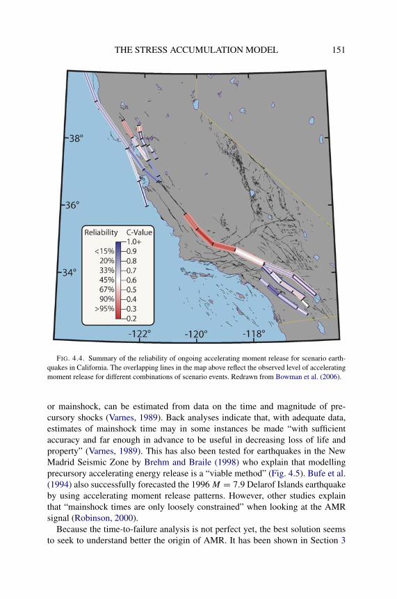
THE STRESS ACCUMULATION MODEL 151
FIG. 4.4. Summary of the reliability of ongoing accelerating moment release for scenario earth-quakes in California. The overlapping lines in the map above reflect the observed level of acceleratingmoment release for different combinations of scenario events. Redrawn from Bowman et al. (2006).
or mainshock, can be estimated from data on the time and magnitude of pre-cursory shocks (Varnes, 1989). Back analyses indicate that, with adequate data,estimates of mainshock time may in some instances be made “with sufficientaccuracy and far enough in advance to be useful in decreasing loss of life andproperty” (Varnes, 1989). This has also been tested for earthquakes in the NewMadrid Seismic Zone by Brehm and Braile (1998) who explain that modellingprecursory accelerating energy release is a “viable method” (Fig. 4.5). Bufe et al.(1994) also successfully forecasted the 1996 M = 7.9 Delarof Islands earthquakeby using accelerating moment release patterns. However, other studies explainthat “mainshock times are only loosely constrained” when looking at the AMRsignal (Robinson, 2000).
Because the time-to-failure analysis is not perfect yet, the best solution seemsto seek to understand better the origin of AMR. It has been shown in Section 3

152M
IGN
AN
(a) (b)
FIG. 4.5. Time-to-failure power-law fit of AMR observed before two earthquakes in the New Madrid Seismic Zone; (a) Precursory sequence for the August1986 M = 3.6 earthquake; (b) Precursory sequence for the April 1989 M = 4.3 earthquake. The solid curve represents the model of AMR with the predictedmainshock time. The dashed curve represents the model of AMR with the actual mainshock time. Redrawn from Brehm and Braile (1998).

THE STRESS ACCUMULATION MODEL 153
that a mathematical formulation for the time-to-failure power-law can be obtainedfrom the Stress Accumulation model. This promising result should, in the future,permit the fit of accelerating moment release to be improved by determining someof the equation parameters from geological and geodetic data (see Section 3 formore detail).
4.2. Accelerating Moment Release and the Sumatra–Java Arc Seismic Hazard
Accelerating moment release is here tested as a precursor of large earthquakesin the view of the Stress Accumulation model. The proposed forecasting methodis used in the case of the Sumatra–Java fault system because of the recent devas-tating consequences of the 2004, Mw = 9.0–9.3 Sumatra earthquake.
Other forecasting methods could also be used, such as algorithm M8 (Keilis-Borok and Rotwain, 1990) or Reverse Tracing of Precursors (Shebalin et al.,2006) that also search for an increase of the seismic activity (see Section 4.1).Pattern Informatics (Tiampo et al., 2006) could also be useful because it catcheschanges of the correlation length, which is implicitly observed in the Stress Ac-cumulation model (Sammis and Sornette, 2002). However the physics underlyingsuch methods remains unclear and it is preferable to base the forecasting plan onaccelerating moment release alone.
This work associates the study of precursory seismicity patterns to the seis-mic cycle of faults and by consequence to the concept of seismic gap. Indeed theStress Accumulation model explains that accelerating moment release is a con-sequence of stable sliding on the faults at depth (see Section 1). Simulations ofKing and Bowman (2003) and the mathematical formulation of accelerating mo-ment release proposed in Section 3 show that this precursor should be observedin the last stages of loading on the fault, before rupture.
The relative role of the Stress Accumulation model and associated acceleratingmoment release in earthquake forecast is illustrated in Fig. 4.6. It shows that theStress Accumulation model provides a complementary information to the study ofrecurrence intervals, independently of possible stress triggering from other earth-quakes on other faults. However, as it will be shown in the Sumatra–Java Arcexample, accelerating moment release does not yet determine the time of occur-rence of the next earthquake. Thus time probabilities cannot yet be determinedfrom this new forecasting method. In this study, a time-to-failure analysis (seeSection 4.1) is not included.
4.2.1. Introduction
The study of the seismic activity in the Sumatra–Java region prior to the De-cember 26, 2004 (Mw = 9.0–9.3) and March 28, 2005 (Mw = 8.7) earthquakesis presented, following Mignan et al. (2006a): A promising approach to assessing
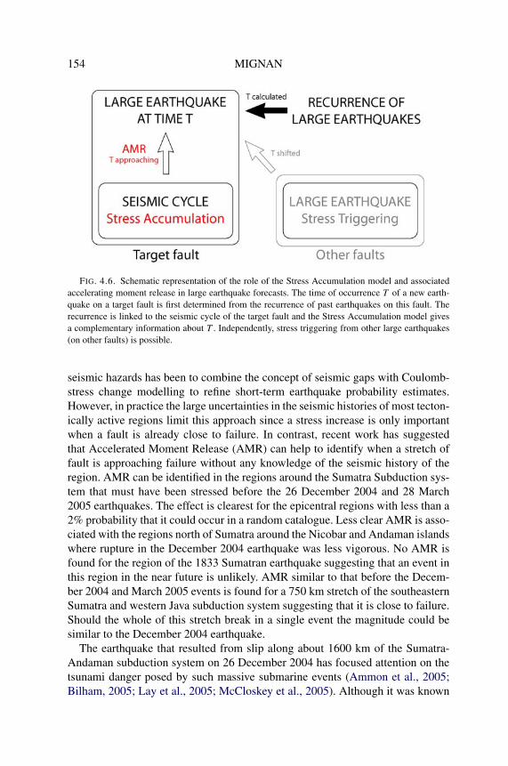
154 MIGNAN
FIG. 4.6. Schematic representation of the role of the Stress Accumulation model and associatedaccelerating moment release in large earthquake forecasts. The time of occurrence T of a new earth-quake on a target fault is first determined from the recurrence of past earthquakes on this fault. Therecurrence is linked to the seismic cycle of the target fault and the Stress Accumulation model givesa complementary information about T . Independently, stress triggering from other large earthquakes(on other faults) is possible.
seismic hazards has been to combine the concept of seismic gaps with Coulomb-stress change modelling to refine short-term earthquake probability estimates.However, in practice the large uncertainties in the seismic histories of most tecton-ically active regions limit this approach since a stress increase is only importantwhen a fault is already close to failure. In contrast, recent work has suggestedthat Accelerated Moment Release (AMR) can help to identify when a stretch offault is approaching failure without any knowledge of the seismic history of theregion. AMR can be identified in the regions around the Sumatra Subduction sys-tem that must have been stressed before the 26 December 2004 and 28 March2005 earthquakes. The effect is clearest for the epicentral regions with less than a2% probability that it could occur in a random catalogue. Less clear AMR is asso-ciated with the regions north of Sumatra around the Nicobar and Andaman islandswhere rupture in the December 2004 earthquake was less vigorous. No AMR isfound for the region of the 1833 Sumatran earthquake suggesting that an event inthis region in the near future is unlikely. AMR similar to that before the Decem-ber 2004 and March 2005 events is found for a 750 km stretch of the southeasternSumatra and western Java subduction system suggesting that it is close to failure.Should the whole of this stretch break in a single event the magnitude could besimilar to the December 2004 earthquake.
The earthquake that resulted from slip along about 1600 km of the Sumatra-Andaman subduction system on 26 December 2004 has focused attention on thetsunami danger posed by such massive submarine events (Ammon et al., 2005;Bilham, 2005; Lay et al., 2005; McCloskey et al., 2005). Although it was known
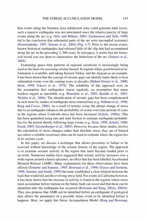
THE STRESS ACCUMULATION MODEL 155
that events along the Sumatra–Java subduction zone could generate tidal waves,such a massive earthquake was not anticipated since the relative paucity of largeevents along the arc (e.g. Ortiz and Bilham, 2003; Zachariasen and Sieh, 1999)led to the conclusion that substantial parts of the arc were uncoupled (aseismic)(Prawirodirdjo, 1997; Simoes et al., 2004) (Fig. 4.7). Prior to the recent events,known historical earthquakes had released little of the slip that had accumulatedalong the arc in the preceding 2–300 years. In retrospect, it seems that the histor-ical record was too short to characterise the behaviour of the arc (Simoes et al.,2004).
Examining space–time patterns of regional seismicity is increasingly beingused as the basis for assessing seismic hazard. In regions where good historical in-formation is available, and taking Eastern Turkey and the Aegean as an example,it has been shown that the concept of seismic gaps can identify faults likely to hostsubstantial events over the coming years or decades (Hubert-Ferrari et al., 2000;Stein, 1999; Toksoz et al., 1979). The reliability of this approach rests onthe assumption that earthquakes repeat regularly, an assumption that manyworkers regard as unreliable (e.g. Benedetti et al., 2002; Rundle et al., 2001;Weldon et al., 2004). The identification of seismic gaps has been complementedin such areas by studies of earthquake stress interactions (e.g. Nalbant et al., 1998;King and Cocco, 2000). As a result of tertiary creep, the abrupt change of stressdue to an earthquake enhances the probability of events over time periods of yearsin the regions where Coulomb-stress has been increased (Scholz, 1990a). Thishas been quantified using rate and state friction to estimate earthquake probabili-ties for the period shortly following large events (e.g. Stein, 1999; Scholz, 1998;Freed, 2005; Gerstenberger et al., 2005). However, because these studies involvethe calculation of stress changes rather than absolute stress, they are of limiteduse unless a reliable recurrence time can be used to estimate where the region liesin its seismic cycle.
In this paper, we discuss a technique that allows proximity to failure to beassessed without knowledge of the seismic history of the region. The approachis to examine seismic activity in the region that must become loaded prior toan event. Numerous studies have suggested that seismic activity increases over awide region around a future epicenter, an effect that has been labelled AcceleratedMoment Release (AMR). Many explanations for these observations have beenoffered (Sornette and Sammis, 1995; Bowman et al., 1998; Grasso and Sornette,1998; Sammis and Smith, 1999) but none established a clear relation between thefault that would fail and the evolving stress field. For events in California however,it has been shown that the increase in activity is found in the regions where stressmust accumulate before motion on the future fault can occur and that these can beidentified after the earthquake has occurred (Bowman and King, 2001a, 2001b).They also propose that AMR can be identified before an earthquake if geologicaldata allows the parameters of a possible future event to be identified before ithappens. Here, we apply this Stress Accumulation Model (King and Bowman,

156 MIGNAN
FIG. 4.7. Large earthquakes (M > 7.5) along the Sumatra–Java arc. Estimated rupture regions forhistorical events are shown in black and the rupture regions for the 26 December 2004 and 28 March2005 are shown in grey.

THE STRESS ACCUMULATION MODEL 157
2003) to the Sumatra–Java arc and demonstrate that the slip regions of both the26 December 2004 and the 28 March 2005 events showed clear evidence that theywere approaching failure prior to the two events. We further show that the regionsof highest slip in the two events correspond to the sections of the arc that exhibitedthe most pronounced AMR. In contrast, the section of the subduction zone wherethe 1833 earthquake occurred shows no reliable evidence of accelerating activityat present. However, a region of accelerating seismicity associated with a 750 kmstretch of the mapped plate boundary along southeastern Sumatra and westernJava suggests that this region may be approaching failure.
4.2.2. The Stress Accumulation Model
The mechanical processes of the Stress Accumulation Model (SAM) are dis-cussed in detail by King and Bowman (2003). They describe a complete seismiccycle for an isolated sticking patch on an otherwise creeping strike-slip fault. Themodel allows synthetic seismic catalogues to be generated that are closely com-parable to those observed. An idealised representation of the evolution of stressand seismicity for the last 10% of the earthquake cycle is shown in Fig. 4.8. Thisis similar to the model described by King and Bowman (2003), but calculated fora reverse fault. The faults adjacent to the impending earthquake are consideredto be early in their seismic cycle and are locked. The fault at depth creeps withslip increasing from 90% to 100% of the slip required to bring the fault in theseismic gap to failure. Figures 4.8a–d represent the last 10, 3.5, 1 and 0% of theseismic cycle. During the last 10% of the cycle, it can be seen that seismic activ-ity (represented by small black dots) rapidly surrounds the future epicentre. Thispattern of activity mimics the so-called “Mogi Doughnut”, a halo of precursoryactivity that is sometimes observed around subduction zone earthquakes (Mogi,1969). Following the earthquake, the stress pattern changes and the location ofthe seismicity switches to the aftershock lobes. King and Bowman (2003) showthat realistic values of earthquake stress drops and stress field inhomogeneitiescan produce artificial catalogues with AMR similar to those observed.
The SAM method (Bowman and King, 2001a, 2001b) defines the region wherestress must accumulate and pre-event seismicity must occur during the last partof the earthquake cycle. The technique is the same as that used to calculate post-earthquake Coulomb-stress (Stein, 1999; King and Cocco, 2000), but the fault isslipped with the opposite sense (the “backslip” model first described by Savage(1983)) to identify the form of the stress field before the earthquake. The formof the stress field is the same for half-space and plate calculations, only the de-cay with distance is changed (Stein et al., 1994). In common with most otherCoulomb stress change studies a half-space calculation is adopted. Figure 4.9shows the method applied to the segment of the subduction zone that experiencedthe largest and most rapid slip in the 26 December 2004 earthquake. The insetshows the surface projection of the fault as a black line. The outlined region cor-

158M
IGN
AN

THE STRESS ACCUMULATION MODEL 159
FIG. 4.8. The evolution of stress and seismicity for the last 10% of the earthquake cycle for areverse fault. The fault geometry (not to scale) is shown in f. The faults adjacent to the impendingearthquake are considered to be early in their seismic cycle and are locked, while the creeping faultat depth increases in slip from 90% to 100% of the slip required to bring the fault in the seismic gapto failure. Since only slip on the fault at depth increases below a locking depth until the earthquakeoccurs, this model is identical to those used to model geodetic data. The values used for the model are7.5 metres slip for the adjacent faults, and the slip on the creeping fault below the seismogenic zoneincreases from 9 to 10 metres. Figures 2(a)–(d) represent the last 10, 3.5, 1 and 0% of the seismiccycle. It can be seen that during the last 10% of the cycle, activity (represented by small black dots)rapidly approaches the future epicentre. Following the earthquake the lobe patterns change and theblack dots represent aftershocks. The mask to provide the inheritance stress (see King and Bowman(2003)) and the colour range are chosen so that failure stress reaches the future fault when deep slipreaches 10 metres. The colour bar shows normalised stress. The depth of the seismogenic zone istaken to be 15 km (locking depth) and the length of the fault is 30 km. To produce the artificialearthquakes, random stress variations (referred to as “noise” in King and Bowman (2003)) are addedto the evolving stress level calculated for realistic earthquake parameters as described above. For thisfigure the random variations are exaggerated to make the events easily visible. It has previously beenshown that, using realistic random variations, a model like this can create artificial seismic cataloguesexhibiting AMR that is similar to real earthquake sequences when analysed by the same methods asreal catalogs (King and Bowman, 2003).
responds to the 0.02 bar coulomb pre-stress contour for the fault parameters givenin the figure caption. The choice of this value is discussed in the next section andin earlier papers (Bowman and King, 2001a, 2001b; Sammis et al., 2004), whereit is pointed out that the form and not the absolute value of stress is of importanceto identify the region that must be loaded prior to an earthquake. The earthquakes(shown by black dots) within this contour demonstrate AMR. The AMR shownin the figure is first identifiable in 1977 with activity steadily increasing until im-mediately prior to the December earthquake. It should be noted that the increasein activity results not from a few larger events near the end of the period but anoverall increase of activity. This provides some support for the view that the AMRis a consequence of a general increase of activity (i.e. an increase of a-value andnot a change of b-value in the Gutenburg–Richter relation) (Stein et al., 1994;Sammis et al., 2004). In this example the backslip earthquake model location andparameters are defined by the reported parameters of the event (Ammon et al.,2005).
To examine AMR along the whole arc we divide it into segments. The quality ofearthquake catalogues in the Sumatra–Java region places a practical constraint onthe size of the segments. In California, where catalogues are complete down to amagnitude of 3.5, it is possible to retrospectively demonstrate AMR before eventsfor M = 6.5 events whose rupture parameters have been established (Bowmanand King, 2001a, 2001b). However, catalogues in the Sumatra–Java region arenot homogeneous below magnitude 4.5, so that it is unreasonable to expect tofind AMR even for known events smaller than M ∼ 7.5 (fault length ∼ 150 km).

160 MIGNAN
FIG. 4.9. Accelerating Moment Release (AMR) for the great Sumatra earthquake of December(12/26/2004). The Cumulative Benioff Strain and the time (in years) are respectively the y-axis andx-axis. The power law fit (dark grey curve) and the line fit (light grey line) used for the calculation ofthe c-value are shown. The c-value is 0.28, which corresponds to a 2% probability that the accelerationcould occur randomly. The pre-stress field calculated by the backslip earthquake method for the highslip part of the 26 December 2004 event is shown in the inset. The grey contour (0.02 bars) outlinesthe area of events that provides the best c-value. Other contours also result in AMR; the one displayedis the optimum. The fault used corresponds to segments 5, 6, and 7 in Table 1. It has a dip of 11◦,a down-dip width of 200 km and each segment is pure dip-slip.
With this constraint in mind, the subduction zone is divided into segments 250km long to search for AMR before future events. This segmentation length meansthat only future events significantly greater than M = 8.0 will be detected.
4.2.3. Quantification of Accelerating Moment Release (AMR)
A number of studies have suggested that AMR can be modelled by fitting asimple power-law time-to-failure equation of the form
(4.5)∑
ε(t) = A + B(tf − t)m
where tf is the time of the large event, B is negative and m is usually about 0.3.A is the value of ε(t) when t = tf (Bowman and Sammis, 2004; Bufe and Varnes,

THE STRESS ACCUMULATION MODEL 161
1993). The cumulative Benioff strain at time t is defined as
(4.6)ε(t) =N(t)∑i=1
√Ei(t)
where Ei is the energy of the ith event and N(t) is the number of events attime t . To quantify the AMR, we use the c-value (Bowman et al., 1998) de-fined to be the ratio between the root mean square of the power-law time-to-failure fit (Eq. (4.5)) and the root mean square of a linear fit to the cumulativeenergy of events. If the c-value tends to zero, a power law best approximatesthe curve and AMR is observed. If the c-value tends to unity then no AMRis seen. For a specified source (known or proposed) the program Nutcracker(http://geology.fullerton.edu/dbowman/downloads/NutcrackerX.1.zip) automati-cally searches for low c-values within a range of Coulomb-stress contours anda range of catalog start times. From this matrix, start times and stress levels canbe identified that exhibit AMR, together with sensitivity of the AMR to parameterchanges.
The stress levels identified in this procedure are used to define the shape of thestressed region (see Fig. 4.9). For any given azimuth, the extent of the pre-stressregion depends on the fault slip. If known fault slip is used following an earth-quake, the stress contours correspond to stress change at the time of the event.Where events have not yet happened, a nominal fault slip is selected and the val-ues of the stress contours should be taken only as a rough guide. Clearly variationsin modulus such as that between ocean and continental crust will modify stresscontours, but such an effect is minor compared to other limitations of the approachaddressed in the discussion.
Since the algorithm automatically seeks regions of low c-value, some degreeof AMR will nearly always be found. To determine if the acceleration is dueto a ‘real’ physical process or is merely a result of random clustering, we haveused the Monte Carlo technique to examine the likelihood of AMR in randomcatalogues. Because any AMR found in these random catalogs cannot be dueto a physical process, they provide a way of estimating the reliability of any giveAMR sequence (Ikeda, 2004) (further information can be found in the Appendix).For the example in Fig. 4.9, the technique suggests that there is less than a 2%possibility that the observed AMR is due to random processes. In the study of theSumatra–Java arc that follows, the reliability of the observed AMR is assessed bydirect observation, examining the start-time versus stress matrix and the c-value(see Appendix). The total time over which the acceleration is observed is also animportant guide. The length of the AMR is related to the length of the seismiccycle (King and Bowman, 2003) and consequently a short total time suggests thatthe AMR is incomplete and the region not yet fully re-stressed. This is consistentwith such regions rupturing only as a consequence of propagation of slip frommore stressed regions (as discussed below). However, an AMR with a short total
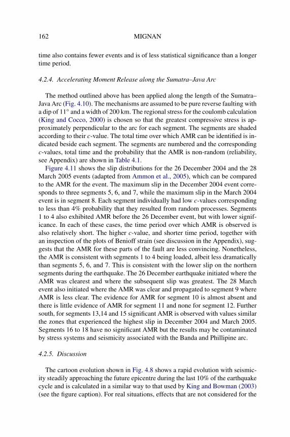
162 MIGNAN
time also contains fewer events and is of less statistical significance than a longertime period.
4.2.4. Accelerating Moment Release along the Sumatra–Java Arc
The method outlined above has been applied along the length of the Sumatra–Java Arc (Fig. 4.10). The mechanisms are assumed to be pure reverse faulting witha dip of 11◦ and a width of 200 km. The regional stress for the coulomb calculation(King and Cocco, 2000) is chosen so that the greatest compressive stress is ap-proximately perpendicular to the arc for each segment. The segments are shadedaccording to their c-value. The total time over which AMR can be identified is in-dicated beside each segment. The segments are numbered and the correspondingc-values, total time and the probability that the AMR is non-random (reliability,see Appendix) are shown in Table 4.1.
Figure 4.11 shows the slip distributions for the 26 December 2004 and the 28March 2005 events (adapted from Ammon et al., 2005), which can be comparedto the AMR for the event. The maximum slip in the December 2004 event corre-sponds to three segments 5, 6, and 7, while the maximum slip in the March 2004event is in segment 8. Each segment individually had low c-values correspondingto less than 4% probability that they resulted from random processes. Segments1 to 4 also exhibited AMR before the 26 December event, but with lower signif-icance. In each of these cases, the time period over which AMR is observed isalso relatively short. The higher c-value, and shorter time period, together withan inspection of the plots of Benioff strain (see discussion in the Appendix), sug-gests that the AMR for these parts of the fault are less convincing. Nonetheless,the AMR is consistent with segments 1 to 4 being loaded, albeit less dramaticallythan segments 5, 6, and 7. This is consistent with the lower slip on the northernsegments during the earthquake. The 26 December earthquake initiated where theAMR was clearest and where the subsequent slip was greatest. The 28 Marchevent also initiated where the AMR was clear and propagated to segment 9 whereAMR is less clear. The evidence for AMR for segment 10 is almost absent andthere is little evidence of AMR for segment 11 and none for segment 12. Furthersouth, for segments 13,14 and 15 significant AMR is observed with values similarthe zones that experienced the highest slip in December 2004 and March 2005.Segments 16 to 18 have no significant AMR but the results may be contaminatedby stress systems and seismicity associated with the Banda and Phillipine arc.
4.2.5. Discussion
The cartoon evolution shown in Fig. 4.8 shows a rapid evolution with seismic-ity steadily approaching the future epicentre during the last 10% of the earthquakecycle and is calculated in a similar way to that used by King and Bowman (2003)(see the figure caption). For real situations, effects that are not considered for the

THE STRESS ACCUMULATION MODEL 163
FIG. 4.10. AMR for the Sumatra–Java arc. For each segment the c-value is indicated and shadedin accordance with the colour bar in the inset. Beside each segment the length of time over whichAMR is identified is indicated in years. The segments are numbered and the corresponding c-values,duration of AMR and probability that the AMR is non-random is shown in Table 4.1. The co-ordinatesof the ends of the segments are also provided. Each segment has a dip of 11◦, a width of 200 km andis pure dip slip with a nominal displacement of 20 metres.

164M
IGN
AN
TABLE 4.1. Segment characteristics. The fault segments all dip at 11◦, a width of 200 km and are pure dip-slip. The regional stress field is chosen accordingly(see text). Since AMR is a far field effect it is not very sensitive to the fault parameters. The reliability is determined from the c-value alone using randomcatalogues (see Appendix). A high reliability and a long total time suggest that the AMR indicates that the segment is loaded. A long total time has no significanceif the reliability is low
Segment Seg startLat◦
Seg startLon◦
Seg endLat◦
Seg endLon◦
c-value Reliability(%)
Total time(yr)
1 (slow rupture associated with the 26 December 2004 event) 93.48 15.58 92.03 13.85 0.46 84 192 (slow rupture associated with the 26 December 2004 event) 92.04 13.85 91.60 11.69 0.51 76 103 (slow rupture associated with the 26 December 2004 event) 91.60 11.69 91.53 9.17 0.35 98 94 (slow rupture associated with the 26 December 2004 event) 91.53 9.17 92.37 7.01 0.44 88 195 (26 December 2004 event) 92.37 7.01 92.86 4.28 0.38 96 286 (26 December 2004 event) 92.86 4.28 94.55 2.92 0.24 99 377 (26 December 2004 event) 95.55 2.92 96.48 1.33 0.29 98 278 (28 March 2005 event) 96.48 1.33 97.30 −0.13 0.33 97 189 (1861 event) 97.30 −0.13 98.26 −1.59 0.60 50 2710 (1833 event) 98.26 −1.59 99.36 −3.19 0.76 23 3211 (1833 event) 99.36 −3.19 100.53 −4.99 0.51 70 3212 (1833 event) 100.53 −4.99 101.97 −6.63 1.0 0 −13 (history unknown) 101.98 −6.63 103.76 −7.93 0.30 98 4014 (history unknown) 103.76 −7.93 105.68 −8.74 0.36 97 4015 (history unknown) 105.68 −8.74 108.28 −9.86 0.37 96 4016 (history unknown) 108.28 −9.86 111.18 −10.21 0.53 76 1417 (history unknown) 111.19 −10.21 114.81 −10.61 0.87 20 3018 (history unknown) 114.81 −10.61 118.38 −10.56 0.64 60 8

THE STRESS ACCUMULATION MODEL 165
FIG. 4.11. Simplified slip distribution for the ruptures of the 26 December 2004 and 28 March2005 earthquakes (modified from Ammon et al. (2005)). The displacements are shown in meters.Grey shading also represents slip with a range from 0 m – white to 10 m – grey.

166 MIGNAN
simple model can intervene. The model supposes that the earthquake cycle con-sists of one simple loading system, where the only elements are creep at depthand the seismic motion of adjacent faults. At the end of the cycle, the stress con-ditions are identical to those at the beginning; the assumptions of a simple elasticrebound model. Elastic rebound concerns only horizontal stresses and displace-ments, however some permanent deformation (topography) is created at the endof the earthquake cycle for a dip-slip fault (King et al., 1988; Stein et al., 1988;Cattin and Avouac, 2000). The flexure, uplift, and subsidence associated withdip-slip earthquakes are associated with their own seismicity, which perturbs thatexpected for an idealised earthquake cycle. In more general terms, complex faultgeometries result in the superposition of the stress fields and associated seismic-ity of multiple faults at different stages in their loading cycles. It is important toappreciate that the strain energy involved in these processes is very small and lo-calised near to the earthquake epicentral region. The strain energy stored prior to,and then released in the main shock, is much greater. For Sumatra geodetic dis-placements of 1 or 2 centimetres occurred in India and Indonesia indicating therelease of stress in a region larger than those in which we identify AMR.
Other major faults or plate boundaries can be associated with stress fields thatare not responsible for the future earthquake. For example, the loading of thestrike-slip fault behind the arc and the associated seismicity involves stress fieldsthat cannot result in the observed dip-slip motion. Since at present such seismicitycannot be separated, events associated with loading of the strike-slip fault couldbe a source of error in the AMR plot for reverse faulting events. A similar situationoccurs for western Java where the Banda and Philippine arcs and associated seis-micity are sufficiently close that they overlap with regions that must be stressedprior to an eastern Java event.
While these sources of error reduce our ability to identify AMR they also offerfuture approaches to improving signal to noise ratios. The most straightforwardwould be to use only precursory events with identified focal mechanisms. Un-fortunately, at present there are few parts of the world where seismic cataloguesboth include mechanisms and are homogeneous. The stress field prior to an eventalso varies with depth in a manner that can readily be calculated to improve theresults. Unfortunately, most earthquake catalogs have poor depth resolution, ren-dering such an approach ineffective. While the limitations of existing cataloguesmust be accepted, future improvements may allow much improved AMR studies.
Prior to the work of King and Bowman (2003), it was assumed that AMR wascorrectly modelled by Eq. (4.5), based on the assumption that the events priorto the earthquake were part of either a failure process or a process analogous toa phase transition. The stress accumulation model (King and Bowman, 2003),in which creep at depth progressively fills a stress shadow, requires that eventsare a symptom of the loading process and are not a part of the failure leading tothe main event. There is consequently no reason to suppose that the main eventshould occur at the asymptote of the failure function. The use of a power law

THE STRESS ACCUMULATION MODEL 167
time-to-failure function (Eq. (4.5)) is used in this study since the filling of thestress shadow cannot be reduced to a simple analytic expression. In the futureit may be possible to generate more appropriate empirical expressions for theAMR. However, in the absence of a clear alternative, Eq. (4.5) is retained onthe understanding that the asymptote has no physical significance. It follows thatsince we do not know at present how much acceleration must be observed beforean earthquake occurs, a clear time prediction is not possible.
The results presented above suggest that part of the southern Sumatra and west-ern Java arc is now subject to similar loading conditions to those that prevailedprior to the Sumatra earthquakes of 26 December 2004 and 28 March 2005. Thedata presented is very suggestive, but would be more certain if we had more exam-ples of AMR before large subduction earthquakes. Unfortunately although verylarge events have occurred (e.g Chile 1960, Alaska 1965) the NEIC catalogue isnot long enough to provide the clear accelerations that span 10’s of years. Whereacceleration is identified over shorter time spans, it is more equivocal.
In the absence of many examples it is uncertain when the southern Sumatraand western Java arc might fail. Models suggest that the most pronounced AMRis within the last 10% of the earthquake cycle (which is perhaps between 200 and500 years for the Sumatra–Java subduction system). AMR should therefore beidentifiable in the last 20 to 50 years before the event. Thus, an AMR total timeof 40 years might suggest that the event will occur in the next few years, but thisis far from certain.
Various workers have proposed that some subduction systems are coupled andseismic, while some are uncoupled and largely aseismic. This has been explainedby mechanical models that invoke parameters including (but not limited to) sub-duction rate, sediment load, and motion of the trench relative to the mantle asdetermining the seismic coupling (Ruff and Kanamori, 1983; Pacheco et al., 1993;Taylor et al., 1996). However, the seismic observations on which these models arebased cover about 100 years, which may not be a sufficiently long time period forthe characterisation of slow subduction systems (Taylor et al., 1996). For both theSumatra (north and central) and Cascadia subduction systems, hitherto regardedas uncoupled, geological investigations have already demonstrated that this isincorrect (Simoes et al., 2004; McCaffrey and Goldfinger, 1995; Clague, 1997;Chlieh et al., 2004). It is therefore pertinent to question the implications of AMRin a subduction setting that has previously been considered to be uncoupled, suchas southern Sumatra and western Java. Certainly the progressive build-up of stressimplied by the stress accumulation model (King and Bowman, 2003) is not consis-tent with steadily creeping subduction. However, recent observations of transientstrain events in subduction settings (e.g. Miller et al., 2002) and theoretical mod-els (Liu and Rice, 2005) although concerning much smaller scales might suggestthat the current period of AMR could be precursory to a non-destructive, slowearthquake.

168 MIGNAN
4.2.6. Conclusion
Parts of the Sumatra–Java arc exhibited clear Accelerated Moment Release(AMR) prior to the 26 December 2004 and 28 March 2005 earthquakes. Onthe basis of a simple loading model of the type widely accepted to explain geo-detic observations (Fig. 4.8 and caption), we propose a model in which the AMRprovides evidence that sections of the arc were approaching failure prior to thecatastrophic events. The method that we use has the potential to directly estimateabsolute stress (relative to failure stress), a significant advance on coulomb stresschange models (King and Cocco, 2000). If demonstrated to be robust, an abilityto independently identify the latter part of the seismic cycle will enhance seismicgap methods of establishing earthquake risk.
The epicentres of both events occurred where AMR, and hence loading, wasgreater and propagated into regions where loading was less. To the south of theslip regions of the recent events, the epicentral area of the 1833 earthquake showsno evidence for an impending earthquake. Recent studies of corals suggest thatthis region is nearing the end of the earthquake cycle (Natawidjaja et al., submit-ted for publication), but the event could still not be close enough for AMR to beobservable yet. However further to the south and east, parts of the Java–Sumatraarc appear to be loaded and may be capable of hosting a devastating earthquake(Fig. 4.12). In the absence of further studies in different regions, a possibility lim-ited by the length of the available seismic catalogues, we cannot be certain thatour results truly indicate an imminent earthquake danger for southeastern Sumatraand western Java. However, our conclusions rest on a simple physical/mechanicalmodel. Bearing in mind the consequences, such an event should be taken seri-ously.
4.2.7. Appendix
Seismic data: The seismicity catalogs required for examining AMR must be ho-mogeneous. Except for a few places, such as California, this can only be satisfiedusing the global catalogue based on the NEIC (ANSS) data set. The catalogueused here was taken from the Advanced National Seismic System (ANSS) World-wide Earthquake Catalog, accessible from the Northern California EarthquakeData Center (http://quake.geo.berkeley.edu/anss), and extended from 01/01/1965to 24/12/04. The minimum magnitude used was 4.5. This was chosen by exam-ining the frequency-magnitude statistics of the catalog to define the minimummagnitude where a stable Gutenberg–Richter relation is observed (Wiemer andWyss, 2000) (e.g. Fig. 4.A1). Because progressive improvements in the globalseismic network have resulted in a progressive lowering of the detection thresh-old of small events, this step is necessary to remove apparent AMR caused bychanging catalog completeness.

THE STRESS ACCUMULATION MODEL 169
FIG. 4.12. The region where observed AMR suggests that the subduction system is approachingthe end of the seismic cycle (light grey).

170 MIGNAN
FIG. 4.A1. The Gutenberg–Richter plot for the data used to calculate AMR along the Suma-tra–Java arc. The catalogue is complete above M 4.5. Subsets of the catalogue in time and space havealso been examined to establish this throughout the region.
Only events with depths from the surface to 40 km were used. This is chosen toinclude those events with depths fixed at 33 km. The stress calculation was carriedout for a depth of 8 km. Since the AMR is associated with seismicity distant fromthe future epicentre this is sufficiently accurate for the range of earthquake depthsconsidered. Deeper events, in particular those associated with the lower part ofthe lithosphere and the subducting slab, may exhibit changes associated with thebuild up of load on the future fault (Astiz et al., 1988; Dmowska et al., 1988;Lay et al., 1989; Dmowska et al., 1996) but would require a three dimensionalstress model and a more complicated search of the stress-time grid. This will beinvestigated in future work.
c-value and statistics: A measure of the reliability of the acceleration in a certainspatiotemporal area in a catalogue of seismicity is carried out by calculating thec-value, which is the ratio between the root mean square of a power law fit andthe root mean square of a linear fit (Bowman et al., 1998). If the c-value tendsto zero, the curve is best approximated by a power law and if the c-value tendsto the unity, the curve can be best approximated by a straight line. Because the

THE STRESS ACCUMULATION MODEL 171
FIG. 4.A2. The probability of different c-values occurring in a random catalogues.
method searches for acceleration data sets may exhibit AMR that has no physicalorigin. To help determine whether an acceleration is likely to be “real” we haveexamined random catalogues of synthetic seismicity.
The Monte Carlo method is used to test the probability that AMR can be founddue to random patterns in seismicity (the “false-alarm rate”). 1000 catalogueseach composed of 500 events placed randomly in space and time are created.Each point is indexed to a magnitude that respects the Gutenberg–Richter law.Energy for each point is calculated using the magnitude-energy scaling law (E =104.8+1.5M ) (Kanamori and Anderson, 1975). This is then used to generate thecumulative Benioff strain curve. When real data is examined, the shape of thespatial region examined depends on the fault mechanism of the earthquake beingexamined. While there is no obvious reason why shape should affect the results,we test the false-alarm rate for circular, square and triangular patterns.
For each geometrical pattern, the search is done using a spatiotemporalmatrix (c-value = f [pattern, distance to the center of the pattern, startingtime]). In detail, for the circle example, events are localised in a unit square[0, 0; 0, 1; 1, 0; 1, 1] and the centre of the circle corresponds to the center of thesynthetic catalog. The calculation of c-value is first done by looking at events lo-cated in a circle of minimum radius (fixed parameter). For these chosen points,another search is done in time by increasing the value of the starting time of thecumulative energy curve (from 0.00 to 0.90 – fixed parameters). This temporalsearch is repeated several times for the spatial search from the minimum radius tothe maximum radius (from 0.05 to 0.50 – fixed parameters). When the c-value is
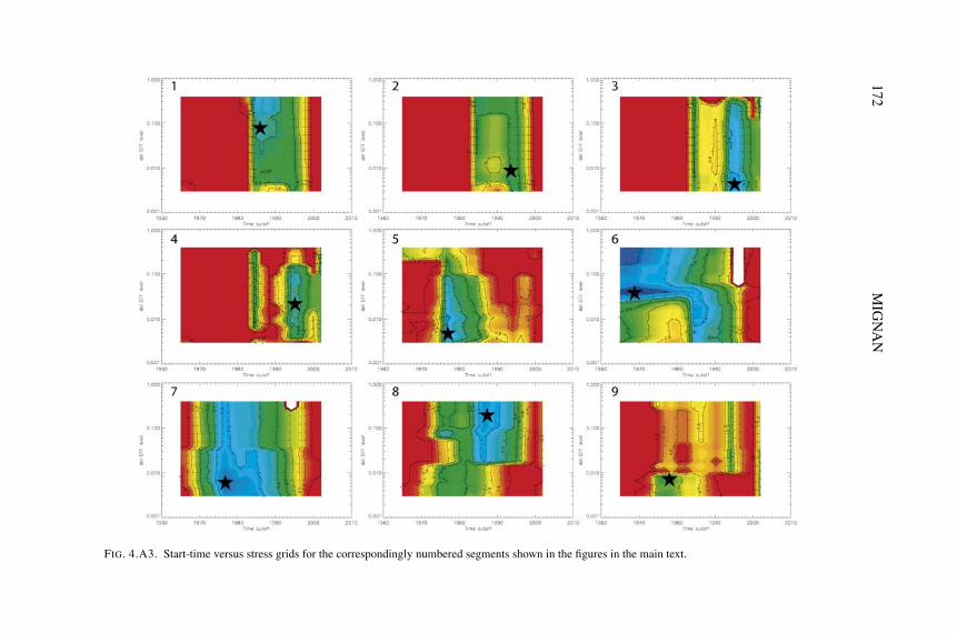
172M
IGN
AN
FIG. 4.A3. Start-time versus stress grids for the correspondingly numbered segments shown in the figures in the main text.

TH
EST
RE
SSA
CC
UM
UL
AT
ION
MO
DE
L173FIG. 4.A3. Continued.

174 MIGNAN
calculated for all increments, the best one is kept (minimum c-value). This is re-peated for each synthetic catalogue and a distribution of minimum c-values is thenobtained. The search using other geometrical patterns adopts the same method bysystematically changing the size of the geometrical figure. The relation betweenthe probability of occurrence and c-value is the same for the three geometriestested, and is shown in Fig. 4.A2.
From the figure it can be concluded that low c-values (< 0.35) are very unlikelyto occur by chance. However, once a c-value of 0.6 is reached the probability thatit could result from random processes is about 50%. In a separate study, differentways of generating random catalogues have been adopted (Ikeda, 2004). Theseinclude randomising the times of real catalogues, using real epicentral distribu-tions and assigning random earthquakes to them, and establishing catalogues thatadopt the ETAS method to simulate aftershocks (Ogata, 1988, 1992). For c-valuesof 0.6 the probability that the observed AMR can be a random effect can increaseto 55%. However for c-values less than 0.35 the probabilities are approximatelyequal to those in Fig. 4.A2. We consequently conclude that c-values less than0.35 have a high probability of being real and those of 0.6 have little significance.As discussed in the text, a low c-value is a necessary condition for determiningwhether an AMR is real. However, it is not a sufficient condition.
Results for all segments: The start-time versus stress grid for all of the segmentsis shown in Fig. 4.A3. The vertical axis shows the Coulomb Stress level and thehorizontal axis the time period. For each combination of Coulomb stress and timerange, the plots indicate the c-value of the associated AMR plot. Light grey indi-cate high c-values and dark grey low c-values. The c-values are also contoured.The best c-value is provided by choosing a dark grey region. In each start-timeversus stress grid, stars indicate the point chosen for the corresponding AMR plotin Fig. 4.A4. In some cases an apparently low c-value can be of little significance.In Fig. 4.A3 for example, the dark grey regions marked bad for segment 1 resultfrom a search very close to the future fault slip; too few events are included to pro-duce a convincing plot. It is important to appreciate that the reliable low c-valuesfor segments 6, 7, 8, 14 and 15 are unambiguous.
4.3. Stability and Reliability of Accelerating Moment Release
The quantification of accelerating moment release by the c-value and its relia-bility have been defined previously (see Section 2 and the previous Section). How-ever different studies show a certain variability of the c-value probability curve
FIG. 4.A4. The AMR plots chosen to be representative for the correspondingly numbered seg-ments shown in the figures in the main text. Information for each segment is provided in Table 1 ofthe main text. The insets indicate the reliability of each plot. See the main text.

TH
EST
RE
SSA
CC
UM
UL
AT
ION
MO
DE
L175

176M
IGN
AN
FIG. 4.A4. Continued.

THE STRESS ACCUMULATION MODEL 177
depending of the method employed (e.g. Bowman et al., 1998; Zoller et al., 2001;Hardebeck et al., in preparation; Mignan et al., 2006a). In this section, a varietyof approaches is first presented and compared to determine the sensitivity of theparameters employed. Because some differences cannot be explained, a new pa-rameter (signal size) is taken into account in the calculation of the reliability ofaccelerating moment release. This gives a better understanding of the differencesobserved in the c-value probability curves. Moreover it gives a more accuratedetermination of the reliability for future forecasting studies.
4.3.1. Previous Studies
A region exhibiting accelerating seismicity has an increased likelihood of alarge earthquake which can be termed an “alarm”. The identification of suchalarms can then be used in forecasting large earthquakes. However, there alwaysexists a finite probability that the observed accelerating moment release in a re-gion is due to random fluctuations in the background seismicity rate, leading toa false alarm. Therefore a c-value probability curve must be determined, whichneeds to define (1) the behaviour of synthetic catalogues and (2) the optimisationprocedure.
Simulation of seismicity catalogues: Ordinary seismic activity corresponds toperiods when there are no peaks of activity perturbing the regional seismicity.Once large earthquakes and associated events (e.g. aftershocks) are removed,ordinary seismicity is composed of random events and clusters in both spaceand time (e.g. Zhuang et al., 2005). A possible representation is the Epidemic-Type Aftershock Sequence model (e.g. Ogata, 1989; Ogata, 1998, see Section 1).However some studies pose the null hypothesis of spatially clustered, tempo-rally random seismicity (e.g. McKernon and Main, 2005). Some others describeseismicity as uniformly random in space and time (e.g. Bowman et al., 1998;Mignan et al., 2006a). The distribution of events on a fractal fault network is alsosometimes considered (e.g. Helmstetter et al., 2005).
Table 4.2 summarises the different random event distributions that can be usedin time and space. The temporal distribution can be random uniform (Poisson
TABLE 4.2. Possible random event distributions intime and space in synthetic seismicity catalogues
Temporal distribution Spatial distribution
random uniform random uniformETAS fractal
cluster-linkedreal cluster

178 MIGNAN
process) or aftershocks can be added (e.g. Zoller et al., 2001; Hardebeck et al.,in preparation). Figure 4.13 represents possible spatial distribution of seismicityevents. In the uniform distribution, events are randomly uniformly distributed inthe space window (Fig. 4.13a). In the fractal distribution, events are localised ina Sierpinski triangle (e.g. Saleur et al., 1996, Fig. 4.13b). In the linked-clusterdistribution, inter-event distances are normally distributed (Fig. 4.13c). It corre-sponds to a modified “random walk” that will produce pseudo-Brownian motion.It can be noted that some studies use a real cluster distribution of events fromreal seismicity catalogues (e.g. Gross and Rundle, 1998; Zoller et al., 2001;Hardebeck et al., in preparation).
The choice of the spatiotemporal distribution of events that compose syntheticcatalogues has consequences for the calculation of the c-value probability curve.However, Ikeda (2004) shows that differences are small (see Fig. 4.14).
Optimisation procedure: The Monte Carlo method is used to calculate the c-valueprobability curve from a large number of synthetic seismicity catalogues. Thehigher the number of used catalogues, the more stable is the result. The optimisa-tion procedure employed must be the same as the one used for real data searches.This can explain some important differences in c-value probability curves. Forexample, probabilities are very low in the study made by Bowman et al. (1998)compared to other ones (e.g. Zoller et al., 2001; Mignan et al., 2006a) because thetime window was fixed whereas more recent studies let the starting time be free.
4.3.2. Signal Size and Stability of Accelerating Moment Release
The differences observed in c-value probability curves cannot be explainedonly by the choice of the behaviour of simulated seismicity and of the optimisationprocedure. Indeed, some important differences are observed in different methodsthat use the same kind of spatiotemporal optimisation (e.g. Zoller et al., 2001;Hardebeck et al., in preparation; Mignan et al., 2006a).
Minimum number of events in the searched pattern: The Monte Carlo method isused for 1000 catalogues composed of 1000 events. Events are random uniformin space and time and respect the Gutenberg–Richter relation. The space windowis optimised for 10 radii and the time window for 10 starting times. For each case,the c-value is calculated only if the number of events in the selected window isgreater than a fixed value (5, 20 or 100 events) otherwise the c-value is fixed at 2.
c-value probability curves are represented in Fig. 4.15. They show that theprobabilities change dramatically depending on the minimum number of eventsthat compose the signal. This can explain why Hardebeck et al. (in preparation)suggest that accelerating moment release is an artifact of data-fitting and does notrepresent a real precursory process. The c-value probability curve that Hardebecket al. (in preparation) propose can be reproduced if accelerating patterns can be

TH
EST
RE
SSA
CC
UM
UL
AT
ION
MO
DE
L179
FIG. 4.13. Possible spatial distributions for a synthetic catalogue composed of 10000 events; (a) uniform distribution; (b) fractal distribution; (c) cluster-linkeddistribution.

180M
IGN
AN
FIG. 4.14. c-value probability curves for different spatiotemporal distributions of events; (a) for random uniform time; (b) for ETAS time. The differentdistributions essentially produce similar results. Redrawn from Ikeda (2004).

THE STRESS ACCUMULATION MODEL 181
FIG. 4.15. c-value probability curves for 1000 catalogues composed of 1000 events. The mini-mum signal-size authorised is 5, 20 and 100 events. Probabilities change dramatically depending ofthe minimum signal size authorised (i.e. number of events that compose the signal).
composed of as few as 5 events. In the work of Mignan et al. (2006a) and Mignanet al. (2006b), the minimum number of events authorised is 15, which shifts thec-value probability curve to higher c-values.
Signal-size distribution: The differences observed in c-value probability curvescan be easily explained by the fact that 5 random points are more likely to forma power-law curve than 15 points or more. Figure 4.16 shows the signal-size dis-tribution for 1000 catalogues composed of 1000 events. Examples of acceleratingpattern (c-value = 0.4) are shown for signals composed of 5, 50 and 400 events.The highest probability (P ∼ 0.4) is obtained for small patterns (composed of ∼5events) and decreases very fast to stabilise at a very low probability (P < 0.01)for signals composed of more than 200 events.
For reasons of stability, the search for accelerating moment release should de-fine at first the minimum size authorised and then calculate the probabilities inconsequence. It can be noted that accelerating moment release found in real caseshave variable “sizes” depending of the methodology employed (see examples inTable 4.3). In the studies of Mignan et al. (2006a) and Mignan et al. (2006b),the largest signals are preferred to smaller ones for reasons of stability. Thisis not the case in other studies (e.g. Bufe et al., 1994; Bowman et al., 1998;Robinson, 2000) where the number of events that compose the signal is not aparameter taken into account in the reliability. The differences observed for Cali-

182 MIGNAN
FIG. 4.16. Signal-size distribution for 1000 catalogues composed of 1000 events. Examples ofaccelerating pattern (c-value = 0.4) are shown for signals composed of 5, 50 and 400 events. Thehighest probability is obtained for small patterns (composed of ∼ 5 events) and decreases very fast tostabilise at a very low probability for signals composed of more than 200 events.
TABLE 4.3. Examples of signal-size for accelerating moment release observed in real seismicitycatalogues
Region Signal-size (# events) Reference
California 30∗ Bufe and Varnes (1993)Alaska 20∗ (6–25) Bufe et al. (1994)California 40∗ (10–100) Bowman et al. (1998)New Madrid Seismic Zone 25∗ (15–40) Brehm and Braile (1998)Aegean region 70∗ (40–90) Papazachos and Papazachos (2000)New Zealand 20∗ (15–30) Robinson (2000)Sumatra 350 Mignan et al. (2006a)California 250 (20–800) Mignan et al. (2006b)
∗Number of events approximated from figures.
fornia data between Bowman et al. (1998) and Mignan et al. (2006b) can also beexplained by different magnitude cutoffs.
To summarise, this study shows that the number of events that compose the sig-nal is of a major importance and should therefore be discussed in future studies.Also it shows that accelerating moment release composed of hundreds of events

THE STRESS ACCUMULATION MODEL 183
FIG. 4.17. Possible outcomes of prediction. For simplicity, the territory where the prediction ismade is represented by a 1D space axis. Rectangles are space–time areas covered by correct (grey) andfalse (white) alarms. Black stars are predicted earthquakes and grey stars, failures to predict. Modifiedfrom Shebalin et al. (2006).
is very unlikely to occur randomly (> 99% of chance that it is a real precursoryprocess).
4.4. Predictability of Earthquakes Using Accelerating Moment Release
Earthquake prediction is commonly defined as specifying the location, time,and magnitude of an impending earthquake within specified ranges (Fig. 4.17).It is important to distinguish between deterministic earthquake predictions andstatistical forecasts. Predictions which are usually specified as deterministic orquasi-deterministic statements, are much more specific, implying considerablyhigher probability and more certainty than a forecast (Kagan and Jackson, 2006).
The “seismic risk map” presented in the case of the Sumatra–Java arc (Sec-tion 4.2) can be considered as a forecasting map. However, it does not directlydetermine the time window of the future large earthquake, but just compares therelative risk on different fault segments and gives an idea of the possible magni-tude. The Stress Accumulation model only gives information about the degree ofloading of a fault that is at the end part of its seismic cycle but is it possible in thefuture to use the Stress Accumulation model to improve forecasting techniques?A discussion about the space-, time-, and magnitude-prediction is made below totry to answer this question.

184 MIGNAN
FIG. 4.18. Overlapping of stress lobes in different fault networks; (a) Schematic representationof the Sumatra–Java Arc subduction zone. If a fault segment is approaching failure (B), accelerat-ing moment release will be observed essentially in the stress lobe associated with this fault segment;(b) Schematic representation of the southern California fault network. If a fault is approaching fail-ure (A), accelerating moment release will be possibly observed in several stress lobes associated withdifferent faults (approaching failure, A or not, B).
4.4.1. Space-Predictable?
The importance of the Stress Accumulation model is that it explains precur-sory seismicity by the behaviour of the stress field around the fault that is goingto fail. By consequence, forecasting methods should focus on each fault that issusceptible to be the origin of a new large earthquake (i.e. space window = faultsegment).
However the spatial distribution of accelerating moment release predicted bythe Stress Accumulation model (see Section 2, Mignan et al., 2006b) shows thatthe stability of results depends on the geometry of active faults. A forecastingmap of the Sumatra–Java Arc (Mignan et al., 2006a) can be proposed because thestress lobe associated with each segment of the fault system only overlaps with thenearby segments (Fig. 4.18a). This is also true for some parts of the San Andreasfault (see Fig. 4.4). In contrast, in the case of Southern California, it is difficult tocreate a forecasting map only based on accelerating moment release. Stress lobesof different faults can overlap and it is not possible to determine which fault willbe the one to fail (Fig. 4.18b).
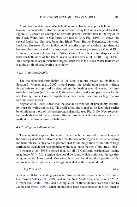
THE STRESS ACCUMULATION MODEL 185
A solution to determine which fault is more likely to approach failure is totake into account other information: other forecasting techniques or geodetic data.Figure 4.19 shows an example of possible present seismic risk in the region ofthe Black Water fault in California (c-value = 0.47, Fig. 4.19a). It shows thatseveral faults (e.g. Garlock, Panamint, Black Water, Harper, Helendale, Lenwood,Lockhart, Emerson, Calico faults) could be at the origin of accelerating seismicitybecause they are located in a large region of precursory seismicity (Fig. 4.19b).However, radar interferometry (InSAR) shows clear interseismic displacementsbetween both sides of the Black Water fault (Peltzer et al. (2001), Fig. 4.19c).This complementary information suggests that this is the Black Water fault whichis at the origin of accelerating seismicity.
4.4.2. Time-Predictable?
The mathematical formulation of the time-to-failure power-law obtained inSection 3 (Mignan et al., 2007) should permit the accelerating moment releasefit analysis to be improved by determining the loading rate. However, the time-to-failure analysis (see Section 4.1) shows variable results and parameters for theaccelerating moment release equation can have large uncertainties (e.g. loadingrate and stress noise).
Mignan et al. (2007) show that the spatial distribution of precursory seismic-ity must be well established. This will allow the signal to be identified earlierby eliminating more of the background seismicity (see Fig. 3.10). New forecast-ing methods should discuss these different problems and determine a statisticalmethod to determine time probabilities.
4.4.3. Magnitude-Predictable?
The magnitude expected for a future event can be determined from the length ofthe fault segment. It can also be noted that the size of the region where acceleratingmoment release is observed is proportional to the magnitude of the future largeearthquake (which can be explained by the relation to the size of the stress lobes).
Bowman et al. (1998) showed that, for all 12 California earthquakes havingmagnitude M � 6.2, a region size could be found which optimised the acceler-ating moment release signal. Moreover, they have found that the logarithm of theradius R of these optimal critical regions scaled as the magnitude M
(4.7)log R ∝ KM
with K = 0.44 the scaling parameter. Similar studies have been carried out inCalifornia (Zoller et al., 2001) and in the New Madrid Seismic Zone (NMSZ)(Brehm and Braile, 1998), and a compilation of these studies has been done byJaumé and Sykes (1999). Other studies have been made outside the USA, such as

186M
IGN
AN
FIG. 4.19. Example of possible present seismic risk in the region of the Black Water fault in California; (a) accelerating moment release from 1960 to2006 (c-value = 0.47); (b) Spatial distribution of accelerating moment release simplified by a circle (radius > 100 km). Stress lobes of different active faultscan overlap the region of possible precursory seismicity (e.g. Garlock, Panamint, Black Water, Harper, Helendale, Lenwood, Lockhart, Emerson, Calico faults);(c) Interseismic displacement between the two sides of the Black Water fault, determined from InSAR, redrawn from Peltzer et al. (2001).

THE STRESS ACCUMULATION MODEL 187
TABLE 4.4. Scaling relation between accelerating moment release critical radii and mainshocks mag-nitude
Scaling K Location Reference
0.44 California (USA) Bowman et al. (1998)0.75 NMSZ (USA) Brehm and Braile (1998)0.36 California & NMSZ (USA) Jaumé and Sykes (1999)0.41 Aegean area Papazachos and Papazachos (2000)0.70 California (USA) Zoller et al. (2001)
FIG. 4.20. Radius-magnitude scaling law. Compilation from different studies (see Table 4.5).
in the Aegean region (Papazachos and Papazachos, 2000). They are presented inTable 4.4.
Sammis and Smith (1999) note that the scaling relation found by Bowman etal. (1998) is compatible with the scaling of preparatory region with magnitudefound by Keilis-Borok and Rotwain (1990) using the algorithm M8. Using thecompilation of previous results and new ones obtained in Section 2 (Table 4.5),the new scaling relation is
(4.8)log R ∝ 0.37M

188 MIGNAN
TABLE 4.5. List of earthquakes with the magnitude/radius relation from different studies
Dateyr/mo/day
Location Mw R
kmReference
1980-02-14 18◦43′N,◦39′W Mw = 4.8 52 Varnes and Bufe (1996)1995-10-31 37.00◦N, 89.40◦W Mw = 6.2 40 Brehm and Braile (1998)1968-11-09 38.00◦N, 88.50◦W Mw = 5.5 120 Brehm and Braile (1998)1975-06-13 36.54◦N, 89.68◦W Mw = 4.3 30 Brehm and Braile (1998)1980-07-05 36.60◦N, 89.58◦W Mw = 3.6 4 Brehm and Braile (1998)1980-12-02 36.21◦N, 89.43◦W Mw = 3.8 4 Brehm and Braile (1998)1983-05-15 38.77◦N, 89.57◦W Mw = 4.3 80 Brehm and Braile (1998)1984-02-14 37.21◦N, 89.00◦W Mw = 3.6 20 Brehm and Braile (1998)1985-12-05 35.90◦N, 90.00◦W Mw = 3.5 20 Brehm and Braile (1998)1986-08-26 38.32◦N, 89.79◦W Mw = 3.6 40 Brehm and Braile (1998)1987-06-10 38.71◦N, 87.95◦W Mw = 5.2 100 Brehm and Braile (1998)1987-06-13 36.58◦N, 89.74◦W Mw = 4.1 5 Brehm and Braile (1998)1987-09-29 36.95◦N, 89.16◦W Mw = 4.3 17 Brehm and Braile (1998)1987-10-14 37.05◦N, 88.78◦W Mw = 3.8 15 Brehm and Braile (1998)1989-04-27 36.09◦N, 89.78◦W Mw = 4.3 5 Brehm and Braile (1998)1990-09-26 37.15◦N, 89.61◦W Mw = 4.8 30 Brehm and Braile (1998)1991-07-07 36.69◦N, 91.57◦W Mw = 3.9 20 Brehm and Braile (1998)1993-01-08 35.93◦N, 90.04◦W Mw = 3.5 6 Brehm and Braile (1998)1994-02-05 37.37◦N, 89.19◦W Mw = 4.2 45 Brehm and Braile (1998)1994-08-20 36.14◦N, 91.06◦W Mw = 3.5 20 Brehm and Braile (1998)1952-07-21 Kern County Mw = 7.5 325 ± 75 Bowman et al. (1998)1992-06-28 Landers Mw = 7.3 150 ± 15 Bowman et al. (1998)1989-10-18 Loma Prieta Mw = 7.0 200 ± 30 Bowman et al. (1998)1994-01-17 Northridge Mw = 6.7 73 ± 17 Bowman et al. (1998)1983-05-02 Coalinga Mw = 6.7 175 ± 10 Bowman et al. (1998)1971-02-09 San Fernando Mw = 6.6 100 ± 20 Bowman et al. (1998)1987-11-24 Superstition Hills Mw = 6.6 275 ± 95 Bowman et al. (1998)1968-04-08 Borrego Mountain Mw = 6.5 240 ± 60 Bowman et al. (1998)1950-08-15 Assam Mw = 8.6 900 ± 175 Bowman et al. (1998)1906-04-18 San Fransisco Mw = 7.7 575 ± 240 Bowman et al. (1998)1986-07-08 Palm Spring Mw = 5.6 40 ± 5 Bowman et al. (1998)1980-02-14 Virgin Islands Mw = 4.8 24 ± 2 Bowman et al. (1998)1948-02-09 35.50◦N, 27.20◦E Mw = 7.1 190 Papazachos and Papazachos (2000)1952-12-17 34.40◦N, 24.50◦E Mw = 7.0 171 Papazachos and Papazachos (2000)1953-03-18 40.02◦N, 27.53◦E Mw = 7.4 246 Papazachos and Papazachos (2000)1953-08-12 38.30◦N, 20.80◦E Mw = 7.2 216 Papazachos and Papazachos (2000)1954-04-30 39.28◦N, 22.29◦E Mw = 7.0 171 Papazachos and Papazachos (2000)1956-07-09 36.64◦N, 25.96◦E Mw = 7.5 284 Papazachos and Papazachos (2000)1957-04-25 36.55◦N, 28.80◦E Mw = 7.2 213 Papazachos and Papazachos (2000)1967-03-04 39.20◦N, 24.60◦E Mw = 6.6 106 Papazachos and Papazachos (2000)1968-02-19 39.50◦N, 25.00◦E Mw = 7.1 157 Papazachos and Papazachos (2000)1970-03-28 39.20◦N, 29.50◦E Mw = 7.1 175 Papazachos and Papazachos (2000)1972-05-04 35.10◦N, 23.60◦E Mw = 6.5 89 Papazachos and Papazachos (2000)1976-05-11 37.40◦N, 20.40◦E Mw = 6.5 131 Papazachos and Papazachos (2000)1979-04-15 42.00◦N, 19.00◦E Mw = 7.1 207 Papazachos and Papazachos (2000)
(continued on next page)

THE STRESS ACCUMULATION MODEL 189
TABLE 4.5. Continued.
Dateyr/mo/day
Location Mw R
kmReference
1981-02-24 38.07◦N, 23.00◦E Mw = 6.7 128 Papazachos and Papazachos (2000)1981-12-19 39.00◦N, 25.26◦E Mw = 7.2 203 Papazachos and Papazachos (2000)1983-01-17 38.10◦N, 20.20◦E Mw = 7.0 171 Papazachos and Papazachos (2000)1986-09-13 37.17◦N, 22.09◦E Mw = 6.0 73 Papazachos and Papazachos (2000)1992-04-30 34.99◦N, 26.72◦E Mw = 6.1 71 Papazachos and Papazachos (2000)1994-09-01 41.12◦N, 21.25◦E Mw = 6.1 61 Papazachos and Papazachos (2000)1995-05-13 40.15◦N, 21.68◦E Mw = 6.6 127 Papazachos and Papazachos (2000)1995-06-15 38.36◦N, 22.28◦E Mw = 6.4 95 Papazachos and Papazachos (2000)1997-10-13 36.33◦N, 22.17◦E Mw = 6.4 92 Papazachos and Papazachos (2000)1997-11-14 38.73◦N, 25.91◦E Mw = 6.0 65 Papazachos and Papazachos (2000)1997-11-18 37.58◦N, 20.57◦E Mw = 6.6 106 Papazachos and Papazachos (2000)1995-02-05 37.65◦S, 179.49◦E Mw = 7.0 167 Robinson (2000)1994-06-18 43.01◦S, 166.71◦E Mw = 6.7 139 Robinson (2000)1993-08-10 45.21◦S, 177.46◦E Mw = 6.7 122 Robinson (2000)1952-07-21 Kern County Mw = 7.5 580 Zoller et al. (2001)1968-04-08 Borrego Mountain Mw = 6.5 60 Zoller et al. (2001)1971-02-09 San Fernando Mw = 6.6 90 Zoller et al. (2001)1983-05-02 Coalinga Mw = 6.7 200 Zoller et al. (2001)1987-11-24 Superstition Hills Mw = 6.6 180 Zoller et al. (2001)1989-10-18 Loma Prieta Mw = 7.0 270 Zoller et al. (2001)1992-06-28 Landers Mw = 7.3 320 Zoller et al. (2001)1994-01-17 Northridge Mw = 6.7 140 Zoller et al. (2001)1999-10-16 Hector Mine Mw = 7.1 180 Zoller et al. (2001)2004-12-26 Sumatra Mw = 9.0 1500 Jiang and Wu (2005)1952-07-21 Kern County Mw = 7.5 102 Mignan et al. (2006b)1968-04-08 Borrego Mountain Mw = 6.5 23 Mignan et al. (2006b)1971-02-09 San Fernando Mw = 6.6 150 Mignan et al. (2006b)1983-05-02 Coalinga Mw = 6.7 90 Mignan et al. (2006b)1987-11-24 Superstition Hills Mw = 6.6 136 Mignan et al. (2006b)1989-10-18 Loma Prieta Mw = 7.0 200 Mignan et al. (2006b)1992-06-28 Landers Mw = 7.3 212 Mignan et al. (2006b)1994-01-17 Northridge Mw = 6.7 231 Mignan et al. (2006b)1999-10-16 Hector Mine Mw = 7.1 228 Mignan et al. (2006b)
and is represented by Fig. 4.20. It can be simply explained in terms of stresstransfer, by relating the magnitude of the future event to the maximum size of thestress lobes, which is in agreement with the Stress Accumulation model.
The Stress Accumulation model permits precursory seismicity to be betterunderstood and thus forecasting may be improved. The spatial distribution of ac-celerating moment release can be specified, the time-to-failure power-law can beaddressed in terms of fault loading and the magnitude can be evaluated from thesize of the stress lobes. As a consequence, a discussion about the reliability ofaccelerating moment release and its relations to the future rupture segment is con-

190 MIGNAN
cevable to determine if a forecast is possible, in which regions and under whatconditions.
GENERAL CONCLUSIONS
“Entities should not be multiplied beyond necessity – or – Of two equivalent theoriesor explanations, all other things being equal, the simpler one is to be preferred.”
W. of Ockham, Occam’s Razor principle (14th century).
The Stress Accumulation model seems to be the best explanation for the originof accelerating moment release observed before large earthquakes.
(1) The spatial distribution of events that compose accelerating moment re-lease fall mainly in regions of increased stress due to loading at depth onthe fault that is going to fail (see Section 2).
(2) The power-law time-to-failure behaviour of accelerating moment releasecan be formulated in simple terms, with the loading rate on the fault (seeSection 3).
This work has shown that the Stress Accumulation model can be defined withsimple stress transfer considerations. Even if criticality concepts can match someaspects of the Stress Accumulation model, this is not needed. At present, a par-allel can be made between accelerating moment release (debated and poorlyunderstood) and aftershocks (accepted and quite well understood), which seemsymmetrical about the mainshock time (acceleration/decceleration). Aftershocksare located in positive stress lobes of the stress field caused by the mainshockwhereas accelerating moment release is located in positive stress lobes of the pre-stress field of the future mainshock. Aftershocks are due to the change of stress atthe time of the mainshock and accelerating moment release is due to the changeof stress during loading before the time of the mainshock. This view permits tobetter understand the possible behaviour of precursory seismicity by defining asimple pattern. This is in contrast with critical concepts where patterns emergefrom chaos and are difficult to catch.
This has important consequences in earthquake forecasting. Indeed many pre-cursors have been proposed, based on different mathematical or statistical toolsaround the criticality concepts. If accelerating moment release is simply definedby the Stress Accumulation model, forecasting is improved. Accelerating momentrelease gives a complementary information to the study of recurrence intervals bythe determination of the degree of loading on the fault, as shown in the case of theSumatra–Java Arc. However, the application of the Stress Accumulation model toearthquake forecasting also shows that a systematic use of accelerating moment

THE STRESS ACCUMULATION MODEL 191
release is complex and depends of the studied region (e.g. fault network geome-try). Also it shows that proper statistics are necessary to correctly determine thereliability of precursory patterns (see Section 4).
This work is a first step to a new understanding of precursory seismicity and toa new technique of large earthquake forecasting. However, time probabilities arenot yet implemented in the Stress Accumulation model and future studies shouldconcentrate on this problem.
ACKNOWLEDGMENTS
Sections 2.1 to 2.5 are the result of collaborative work with David D. Bowman(California State Univ., Fullerton), and Geoffrey C.P. King (Inst. Phys. Globe,Paris) (Mignan et al., 2006b). We are grateful for comments on the work by Rus-sel Robinson, Kristy Tampo, and Steven Cohen, and for support by the FrenchINSU-CNRS and the Southern California Earthquake Center, funded by USANSF Cooperative Agreement EAR-0106924 and USGS Cooperative Agreement02HQAG0008.
Sections 3.2.1 to 3.2.4 are the result of collaborative work with Geoffrey C.P.King and David D. Bowman (Mignan et al., 2007). We are grateful to CharlesSammis, John Rundle, Steven Cohen, and Renata Dmowska for helpful sugges-tions and critical comments, and for support by the same sources.
Sections 4.2.1 to 4.2.7 are the result of collaborative work with Geoffrey C.P.King, David D. Bowman, Robin Lacassin (Inst. Phys. Globe, Paris), and RenataDmowska (Harvard Univ.) (Mignan et al., 2006a). We are grateful to Paul Tappon-nier and James R. Rice for helpful suggestions and critical comments, to RogerBilham for extensive commentary that substantially improved an early presenta-tion of the results, and for support by the same sources.
The author acknowledges helpful reviews by Basil Papazachos and CharlesSammis. The author also thanks Geoffrey King, David Bowman, Renata Dmow-ska, Robert Muir-Wood and Raoul Madariaga for helpful suggestions and criticalcomments.
REFERENCES
Aki, K., Richards, P. (1980). Quantitative Seismology. W.H. Freeman and Co., San Francisco.Allegre, C.J., Le Mouel, J.L., Provost, A. (1982). Scaling rules in rock fracture and possible implica-
tions for earthquake predictions. Nature 297, 47–49.Ammon, C.J., et al. (2005). Rupture process of the 2004 Sumatra–Andaman earthquake. Science 308,
1133–1139.Astiz, L., Lay, T., Kanamori, H. (1988). Large intermediate-depth earthquakes and the subduction
process. Phys. Earth Planet. Int. 53, 80–166, doi:10.1016/0031-9201(88)90138-0.

192 MIGNAN
Bak, P., Paczuski, M. (1995). Complexity, contingency, and criticality. Colloquium Proc. Natl. Acad.Sci. USA 92, 6689–6696.
Bak, P., Tang, C. (1989). Earthquakes as a self-organized critical phenomenon. J. Geophys. Res. 94,15635–15637.
Bak, P., Tang, C., Wiesenfeld, K. (1987). Self-organized criticality: An explanation of the 1/f noise.Phys. Rev. Lett. 59, 381–384.
Bak, P., Tang, C., Wiesenfeld, K. (1988). Self-organized criticality. Phys. Rev. A 38, 364–374.Bakun, W.H., McEvilly, T.V. (1984). Recurrence models and the Parkfield, California, earthquakes.
J. Geophys. Res. 89, 3051–3058.Barka, A. (1999). The 17 August 1999 Izmit earthquake. Science 285, 1858–1859.Ben-Zion, Y., Lyakhovsky, V. (2002). Accelerated seismic release and related aspects of seismicity
patterns on earthquake faults. Pure Appl. Geophys. 159, 2385–2412.Benedetti, L., Finkel, R., Papanastassiou, D., King, G.C.P., Armijo, R., Ryerson, F.J., Farber, D.,
Flerit, F. (2002). Post-glacial slip history of the Sparta fault (Greece) determined by36Cl cosmogenic dating: evidence for non-periodic earthquakes. Geophys. Res. Lett. 10,doi:10.1029/2001GL014510.
Beroza, G.C., Zoback, M.D. (1993). Mechanism diversity of the Loma Prieta aftershocks and themechanics of mainshock-aftershock interaction. Science 259, 210–213.
Bilham, R. (2005). A flying start, then a slow slip. Science 305, 1126–1127.Blanter, E.M., Shnirman, M.G., Le Mouel, J.L. (1997). Hierarchical model of seismicity: scaling and
predictability. Phys. Earth Planet. Int. 103, 135–150.Bowman, D.D., King, G.C.P. (2001a). Accelerating seismicity and stress accumulation before large
earthquakes. Geophys. Res. Lett. 28, 4039–4042, doi:10.1029/2001GL013022.Bowman, D.D., King, G.C.P. (2001b). Stress transfer and seismicity changes before large earthquakes,
Earth. Planet. Sci. Lett. 333, 591–599.Bowman, D., Sammis, C.G. (2004). Intermittent criticality and the Gutenberg–Richter distribution.
Pure Appl. Geophys. 161, 1945–1956.Bowman, D., Ouillon, G., Sammis, C., Sornette, A., Sornette, D. (1998). An observational test of the
critical earthquake concept. J. Geophys. Res. 103, 24359–24372.Bowman, D., Colella, H., Tiampo, K. (2006). Seismicity rate changes and earthquake forecasting
beyond the San Andreas. 100th Anniversarry Earthquake Conference, USA.Brehm, D.J., Braile, L.W. (1998). Intermediate-term earthquake prediction using precursory events in
the New Madrid seismic zone. Bull. Seismol. Soc. Am. 88, 564–580.Bufe, C.G., Varnes, D.J. (1993). Predictive modeling of the seismic cycle of the greater San Francisco
Bay region. J. Geophys. Res. 98, 9871–9883.Bufe, C.G., Nishenko, S.P., Varnes, D.J. (1994). Seismicity trends and potential for large earthquakes
in the Alaska–Aleutian region. Pure Appl. Geophys. 142, 83–99.Carlson, J.M., Langer, J.S. (1989). Properties of earthquakes generated by fault dynamics. Phys. Rev.
Lett. 62, 2632–2635.Cattin, R., Avouac, J.P. (2000). Modelling mountain building and the seismic cycle in the Himalaya
of Nepal. J. Geophys. Res. 105, 13389–14407.Chlieh, M., Avouac, J., Sieh, K., Natawidjaja, D.H., Galetzka, J. (2004). Investigating lateral varia-
tions of interseismic strain along the Sumatran subduction zone. In: AGU Fall Meeting Abstracts,pp. C1385+.
Clague, J.J. (1997). Evidence for large earthquakes at the Cascadia subduction zone. Rev. Geophys. 35,doi:10.1029/97RG00222.
Clark, J., Bowman, D., King, G., Sammis C. (2003). Accelerating moment release as a tool for seismichazard assessment in southern California. In: EGS–AGU–EUG Joint Assembly, Abstracts from themeeting held in Nice, France, 6–11 April 2003, abstract #7422, pp. 7422-+.
Cocco, M., Nostro, C., Ekstrom, G. (2000). Static stress changes and fault interaction during the 1997Umbria-Marche earthquake sequence. J. Seismol. 4, 501–516.

THE STRESS ACCUMULATION MODEL 193
Das, S., Scholz, C.H. (1981). Theory of time-dependent rupture in the earth. J. Geophys. Res. 86,6039–6051.
Deng, J., Sykes, L.R. (1997). Stress evolution in southern California and triggering of moderate-,small-, and micro-size earthquakes. J. Geophys. Res. 102, 24411.
Dieterich, J. (1994). A constitutive law for rate of earthquake production and its application to earth-quake clustering. J. Geophys. Res. 99, 2601–2618.
Dieterich, J., Kilgore, B. (1996). Implications of fault constitutive properties for earthquake prediction.Proc. Natl. Acad. Sci. USA 93, 3787–3794.
Dmowska, R., Rice, J.R., Lovison, L.C., Josell, D. (1988). Stress transfer and seismic phenomena incoupled subduction zones during the earthquake cycle. J. Geophys. Res. 93, 7869–7884.
Dmowska, R., Zheng, G., Rice, J.R. (1996). Seismicity and deformation at convergent margins due toheterogeneous coupling. J. Geophys. Res. 101, 3015–3029.
Fedotov, S.A. (1968). The seismic cycle, quantitative seismic zoning, and long-term seismic forecast-ing. In: Medvedev, S. (Ed.), Seismic Zoning of the USSR, pp. 133–166.
Felzer, K.R., Brodsky, E.E. (2005). Testing the stress shadow hypothesis. J. Geophys. Res. 110,doi:10.1029/2004JB003277.
Freed, A.M. (2005). Earthquake triggering by static, dynamic and postseismic stress transfer. Annu.Rev. Earth Planet. Sci. 33, 335–367.
Gabrielov, A., Zaliapin, I., Newman, W.I., Keilis-Borok, V.I. (2000). Colliding cascades model forearthquake prediction. Geophys. J. Int. 143, 427–437.
Geller, R.J., Jackson, D.D., Kagan, Y., Mulargia, F. (1997). Earthquakes cannot be predicted. Sci-ence 275, 1616–1617.
Gerstenberger, M.C., Wiemer, S., Jones, L.M., Reasenberg, P.A. (2005). Real-time forecasts of tomor-row’s earthquakes in California. Nature 435, 328–331.
Gomberg, J., Blanpied, M.L., Beeler, N.M. (1997). Transient triggering of near and distant earth-quakes. Bull. Seismol. Soc. Am. 87, 294–309.
Gomberg, J., Beeler, N.M., Blanpied, M.L., Bodin, P. (1998). Earthquake triggering by transient andstatic deformations. J. Geophys. Res. 103, 24411–24426, doi:10.1029/98JB01125.
Gomberg, J., Belardinelli, M.E., Cocco, M., Reasenberg, P. (2005). Time-dependent earthquake prob-abilities. J. Geophys. Res. 110, doi:10.1029/2004JB003405.
Grasso, J.R., Sornette, D. (1998). Testing self-organized criticality by induced seismicity. J. Geophys.Res. 103, 2965–2988.
Gross, S., Kisslinger, C. (1997). Estimating tectonic stress rate and state with Landers aftershocks.J. Geophys. Res. 102, 7603.
Gross, S., Rundle, J. (1998). A systematic test of time-to-failure analysis. Geophys. J. Int. 133, 57–64.Gutenberg, B., Richter, C.F. (1956). In: Seismicity of the Earth and Associated Phenomena. Princeton
University Press, p. 310.Hainzl, S., Zoller, G., Kurths, J., Zshau, J. (2000). Seismic quiescence as an indicator for large earth-
quakes in a system of self-organized criticality. Geophys. Res. Lett. 27, 597–600.Hardebeck, J.L. (2004). Stress triggering and earthquake probability estimates. J. Geophys. Res. 109,
4310, doi:10.1029/2003JB002437.Hardebeck, J.L., Felzer, K.R, Michael, A.J. (in preparation). Rigorous observational tests contradict
the accelerating moment release hypothesis.Hardebeck, J.L., Nazareth, J.J., Hauksson, E. (1998). The static stress change triggering model: Con-
straints from two southern California aftershock sequences. J. Geophys. Res. 103, 24427–24438,doi:10.1029/98JB00573.
Harris, R.A. (1998). Introduction to special section: Stress triggers, stress shadows, and implicationsfor seismic hazard. J. Geophys. Res. 103, 24347–24358.
Harris, R.A., Simpson, R.W. (1993). In the shadow of 1857; an evaluation of the static stress changesgenerated by the M8 Ft. Tejon, California earthquake. EOS Trans. AGU 74 (Fall Meet. Suppl.),427.

194 MIGNAN
Harris, R.A., Simpson, R.W. (1996). In the shadow of 1857; the effect of the great Ft. Tejon earthquakeon subsequent earthquakes in Southern California. Geophys. Res. Lett. 23, 229–232.
Harris, R.A., Simpson, R.W. (1998). Suppression of large earthquakes by stress shadows:A comparison of Coulomb and rate-and-state failure. J. Geophys. Res. 103, 24439–24452,doi:10.1029/98JB00793.
Harris, R.A., Simpson, R.W. (2002). The 1999 Mw 7.1 Hector Mine, California, earthquake: A testfor the stress shadow hypothesis? Bull. Seismol. Soc. Am. 92, 1497–1512.
Harris, R.A., Simpson, R.W., Reasenberg, P. (1995). Influence of static stress changes on earthquakelocations in Southern California. Nature 375, 221–224.
Helmstetter, A. (2003). Is earthquake triggering driven by small earthquakes?. Phys. Rev. Lett. 91,058501, doi:10.1103/PhysRevLett.91.058501.
Helmstetter, A., Sornette, D. (2002). Subcritical and supercritical regimes in epidemic models of earth-quake aftershocks. J. Geophys. Res. 107, doi:10.1029/2001JB001580.
Helmstetter, A., Sornette, D., Grasso, J.R. (2003). Mainshocks are aftershocks of conditional fore-shocks: How do foreshock statistical properties emerge from aftershock laws. J. Geophys.Res. 108.
Helmstetter, A., Kagan, Y.Y., Jackson, D.D. (2005). Importance of small earthquakes for stress trans-fers and earthquake triggering. J. Geophys. Res. 110, doi:10.1029/2004JB003286.
Holliday, J.R., Rundle, J.B., Tiampo, K.F., Klein, W., Donnelan, A. (2006). Modification of the patterninformatics method for forecasting large earthquake events using complex eigenfactors. Tectono-physics 413, 87–91.
Hough, S.E. (2002). Earthshaking Science. Princeton University Press.Huang, Y., Saleur, H., Sammis, C., Sornette, D. (1998). Precursors, aftershocks, criticality and self-
organized criticality. Europhys. Lett. 41, 43–48.Hubert-Ferrari, A., Barka, A., Jacques, E., Nalbant, S.S., Meyer, B., Armijo, R., Tapponnier, P., King,
G.C.P. (2000). Seismic hazard in the Marmara Sea region following the 17 August 1999 Izmitearthquake. Nature 404, 269–273.
Hubert-Ferrari, A., King, G., Manighetti, I., Armijo, R., Meyer, B., Tapponnier, P. (2003). Long-termelasticity in the continental lithosphere; Modelling the Aden Ridge propagation and the Anatolianextrusion process. Geophys. J. Int. 153, doi:10.1046/j.1365-246X.2003.01872.x.
Ikeda, N. (2004). Testing the false alarm rate of accelerating moment release before large earthquakes.M.S. Thesis, Cal. State Univ. Fullerton.
Ishimoto, M., Ida, K. (1939). Observations of earthquakes registered with the microseismograph con-structed recently. Bull. Earthq. Res. Inst. 17, 443–478.
Jacques, E., King, G.C.P., Tapponnier, P., Ruegg, J.C., Manighetti, I. (1996). Seismic activity triggeredby stress changes after the 1978 events in the Asal Rift, Djibouti. Geophys. Res. Lett. 88, 2481–2484.
Jaumé, S.C., Estabrook, C.H. (1992). Accelerating seismic moment release and outer-rise compres-sion: Possible precursors to the next great earthquake in the Alaska Peninsula region. Geophys.Res. Lett. 19, 345–348.
Jaumé, S.C., Sykes, L.R. (1999). Evolving towards a critical point: A review of accelerating seismicmoment/energy release prior to large and great earthquakes. Pure Appl. Geophys. 155, 279–305.
Jiang, C.-S., Wu, Z.-L. (2005). The December 26, 2004, off the west coast of northern Sumatra,Indonesia, Mw = 9.0, earthquake and the critical-point-like model of earthquake preparation.Acta Seismol. Sinica 18, 290–296.
Joswig, M. (2001). Mapping seismic quiescence in California. Bull. Seismol. Soc. Am. 91, 64–81.Kagan, Y.Y., Jackson, D.D. (2006). Comment on “Testing earthquake prediction methods: The West
Pacific short-term forecast of earthquakes with magnitude MwHRV � 5.8” by V.G. Kossobokov.Tectonophysics 413, 33–38.
Kagan, Y.Y., Knopoff, L. (1987). Statistical short-term earthquake prediction. Science 236, 1563–1567.

THE STRESS ACCUMULATION MODEL 195
Kagan, Y.Y., Jackson, D.D., Liu, Z. (2005). Stress and earthquakes in southern California: 1850–2004.J. Geophys. Res. 110, 1850–2004.
Kanamori, H., Anderson, D.L. (1975). Theoretical basis of some empirical relations in seismology.Bull. Seismol. Soc. Am. 65, 1073–1095.
Karakaisis, G.F., Papazachos, C.B., Savvaidis, A.S., Papazachos, B.C. (2002). Accelerating seismiccrustal deformation in the North Aegean Trough, Greece. Geophys. J. Int. 148, 193–200.
Karakaisis, G.F., Papazachos, C.B., Scordilis, E.M., Papazachos, B.C. (2004). Current acceleratingseismic excitation along the northern boundary of the Aegean Microplate. Tectonophysics 383, 81.
Karakostas, V.G., Papadimitriou, E.E., Karakaisis, G.F., Papazachos, C.B., Scordilis, E.M., Varge-mezis, G., Aidona, E. (2003). The 2001 Skyros, Northern Aegean, Greece, earthquake sequence:off-fault aftershocks, tectonic implications, and seismicity triggering. Geophys. Res. Lett. 30,doi:10.1029/2002GL015814.
Karakostas, V.G., Papadimitriou, E.E., Papazachos, C.B. (2004). Properties of the 2003 Lefkada,Ionian Islands, Greece, earthquake seismic sequence and seismicity triggering. Bull. Seismol. Soc.Am. 94, 1976–1981.
Katsumata, K., Kasahara, M. (1999). Precursory seismic quiescence before the 1994 Kurile earthquake(Mw = 8.3) revealed by three independent seismic catalogs. Pure Appl. Geophys. 155, 443–470.
Keilis-Borok, V.I. (1996). Intermediate-term earthquake prediction. Proc. Natl. Acad. Sci. USA 93,3748–3755.
Keilis-Borok, V.I., Kossobokov, V.G. (1990). Premonitory activation of earthquake flow: algo-rithm M8. Phys. Earth Planet. Int. 61, 73–83, doi:10.1016/0031-9201(90)90096-G.
Keilis-Borok, V.I., Rotwain, I.M. (1990). Diagnosis of time of increased probability of strong earth-quakes in different regions of the world: algorithm CN. Phys. Earth Planet. Int. 61, 57–72,doi:10.1016/0031-9201(90)90095-F.
Keilis-Borok, V.I., Ismail-Zadeh, A., Kossobokov, V., Shebalin, P. (2001). Non-linear dynamics of thelithosphere and intermediate-term earthquake prediction. Tectonophysics 338, 247–260.
Kenner, S., Segall, P. (1999). Time-dependence of the stress shadowing effect and its relation to thestructure of the lower crust. Geology 27, 119–122.
Kerr, R.A. (1993). Parkfield quakes skip a beat. Science 259, 1120–1123.Kilb, D., Ellis, M., Gomberg, J., Davis, S. (1997). On the origin of diverse aftershock mechanisms
following the 1989 Loma Prieta earthquake. Geophys. J. Int. 128, 557–570.King, G. (1983). The accommodation of large strains in the upper lithosphere of the earth and other
solids by self-similar fault systems: the geometrical origin of b-value. Pure Appl. Geophys. 121,761–815.
King, G.C.P., Bowman, D. (2003). The evolution of regional seismicity between large earthquakes.J. Geophys. Res. 108, doi:10.1029/2001JB000783.
King, G.C.P., Cocco, M. (2000). Fault interaction by elastic stress changes: new clues from earthquakesequences. Adv. Geophys. 44, 1–38.
King, G.C.P., Stein, R.S., Rundle, J.B. (1988). The growth of geological structures by repeated earth-quakes 1. Conceptual framework. J. Geophys. Res. 93, 307–313.
King, G.C.P., Stein, R.S., Lin, J. (1994). Static stress changes and the triggering of earthquakes. Bull.Seismol. Soc. Am. 84, 935–953.
Kisslinger, C. (1996). Aftershocks and fault-zone properties. Adv. Geophys. 38, 1–36.Knopoff, L., Levshina, T., Keilis-Borok, V., Mattoni, C. (1996). Increased long-range intermediate-
magnitude earthquake activity prior to strong earthquakes in California. J. Geophys. Res. 101,5779–5796.
Kossobokov, V.G., Keilis-Borok, V.I., Smith, S.W. (1990). Localization of intermediate-term earth-quake prediction. J. Geophys. Res. 95, 19763–19772.
Kossobokov, V.G., Romashkova, L.L., Keilis-Borok, V.I., Healy, J.H. (1999). Testing earthquake pre-diction algorithms: statistically significant advance prediction of the largest earthquakes in theCircum-Pacific, 1992–1997. Phys. Earth Planet. Int. 111, 187–196.
196 MIGNAN
Lay, T., Astiz, L., Kanamori, H., Christensen, D.H. (1989). Temporal variation of large intraplateearthquakes in coupled subduction zones. Phys. Earth Planet. Int. 54, 258–312, doi:10.1016/0031-9201(89)90247-1.
Lay, T., et al. (2005). The great Sumatra–Andaman earthquake of 26 December 2004. Science 308,1127–1133.
Levin, S.Z., Sammis, C.G., Bowman, D.D. (2006). An observational test of the stress accumulationmodel based on seismicity preceding the 1992 Landers, CA earthquake. Tectonophysics 413, 39–52.
Lienkaemper, J.J., Galehouse, J.S., Simpson, R.W. (1997). Creep response of the Hayward fault tostress changes caused by the Loma Prieta earthquake. Science 276, 2014–2016.
Lin, A., Stein, R.S. (2004). Stress triggering in thrust and subduction earthquakes and stress interac-tions between the southern San Andreas and nearby thrust and strike slip faults.
Liu, Y., Rice, J.R. (2005). Aseismic slip transients emerge spontaneously in 3D rate and state modelingof subduction earthquake sequences. J. Geophys. Res. 110, doi:10.1029/2004JB003424.
Lyakhovsky, V., Ben-Zion, Y., Agnon, A. (1997). Distributed damage, faulting, and friction. J. Geo-phys. Res. 102, 27635–27650, doi:10.1029/97JB01896.
Ma, K.F., Chang, C.H., Stein, R.S. (2005). Response of seismicity of Coulomb stress triggers andshadows of the 1999 M (sub w) = 7.6 Chi-chi, Taiwan, earthquake. J. Geophys. Res. 110,doi:10.1029/2004JB003389.
Main, I.G., Meredith, P.G. (1989). Classification of earthquake precursors from a fracture mechanicsmodel. Tectonophysics 167, 273–283.
Matsuura, M., Jackson, D.D., Cheng, A. (1986). Dislocation model for aseismic crustal deformationat Hollister, California. J. Geophys. Res. 91, 12661–12674.
Matthews, M.V., Ellsworth, W.L., Reasenberg, P.A. (2002). A Brownian model for recurrent earth-quakes. Bull. Seismol. Soc. Am. 92, 2233–2250.
McCaffrey, R., Goldfinger, C. (1995). Forearc deformation and great subduction earthquakes: Impli-cations for cascadia offshore earthquake potential. Science 267, 856–859.
McCloskey, J., Nalbant, S.S., Steacy, S. (2005). Earthquake risk from co-seismic stress. Nature 434,291.
McKernon, C., Main, I.G. (2005). Regional variations in the diffusion of triggered seismicity. J. Geo-phys. Res. 110, doi:10.1029/2004JB003387.
Meyer, B., Tapponnier, P., Bourjot, L., Métivier, F., Gaudemer, Y., Peltzer, G., Guo, S., Chen, Z.(1998). Crustal thickening in Gansu-Qinghai, lithospheric mantle subduction, and oblique, strike-slip controlled growth of the Tibet Plateau. Geophys. J. Int. 135, 1–47.
Mignan, A., King, G.C.P., Bowman, D. (2007). A mathematical formulation of accelerating momentrelease based on the stress accumulation model. J. Geophys. Res. 112, doi:10.1029/2006JB004671.
Mignan, A., King, G.C.P., Bowman, D., Lacassin, R., Dmowska, R. (2006a). Seismic activity in theSumatra–Java region prior to the December 26, 2004 (Mw = 9.0–9.3) and March 28, 2005(Mw = 8.7) earthquakes. Earth. Planet. Sci. Lett. 244, 639–654.
Mignan, A., Bowman, D., King, G.C.P. (2006b). An observational test of the origin of acceleratingmoment release before large earthquakes. J. Geophys. Res. 111, doi:10.1029/2006JB004374.
Miller, M., Melbourne, T., Johnson, D.J., Summer, W.Q. (2002). Periodic slow earthquakes from theCascadia subduction zone. Science 295, 2423.
Mogi, K. (1969). Some features of recent seismic activity in and near Japan (2), Activity before andafter large earthquakes. Bull. Earthquake Research Institute, University of Tokyo 47, 395–417.
Mogi, K. (1981). Earthquake prediction program in Japan. In: Simpson, D.W., Richards, P.G. (Eds.),Earthquake Prediction: An International Review. American Geophysical Union, Washington, DC,pp. 635–666.
Nalbant, S.S., Hubert, A., King, G.C.P. (1998). Stress coupling between earthquakes in northwestTurkey and the north Aegean Sea. J. Geophys. Res. 103, 24469–24486, doi:10.1029/98JB01491.

THE STRESS ACCUMULATION MODEL 197
Natawidjaja, D., Sieh, K., Galetzka, J., Suwargadi, B., Chlieh, M., Cheng, H., Edwards, R.L., Avouac,J.P., Ward, S. (submitted for publication). The giant Sumatran megathrust ruptures of 1797 and1833: paleoseismic evidence from coral microatolls. J. Geophys. Res.
Newman, W.I., Phoenix, S.L. (2001). Time-dependent fiber-bundles with local load sharing. Phys.Rev. E 63, 021507.
Nishenko, S.P., Bollinger, G.A. (1990). Forecasting damaging earthquakes in the Central and EasternUnited States. Science 249, 1412–1416.
Nishenko, S.P., Buland, R. (1987). A generic recurrence interval distribution for earthquake forecast-ing. Bull. Seismol. Soc. Am. 77, 1382–1399.
Nostro, C., Chiaraluce, L., Cocco, M., Baumont, D., Scotti, O. (2005). Coulomb stress changes causedby repeated normal faulting earthquakes during the 1997 Umbria-Marche (central Italy) seismicsequence. J. Geophys. Res. 110, doi:10.1029/2004JB003386.
Ogata, Y. (1988). Statistical models for earthquake occurrences and residual analysis for pointprocesses. J. Am. Stat. Assoc. 83, 9–27.
Ogata, Y. (1989). Statistical model for standard seismicity and detection of anomalies by residualanalysis. Tectonophysics 169, 159–174.
Ogata, Y. (1992). Detection of precursory relative quiescence before great earthquakes through a sta-tistical model. J. Geophys. Res. 97, 19845.
Ogata, Y. (1998). Space–time point-process models for earthquake occurrences. Ann. Inst. Stat.Math. 50, 379–402.
Ogata, Y. (1999). Estimating the hazard of rupture using uncertain occurrence times of pale-oearthquakes. J. Geophys. Res. 104, 17995–18014.
Ogata, Y. (2005). Detection of anomalous seismicity as a stress change sensor. J. Geophys. Res. 110,doi:10.1029/2004JB003245.
Ogata, Y., Zhuang, J. (2006). Space-time ETAS models and an improved extension. Tectono-physics 413, 13–23.
Ogata, Y., Jones, L.M., Toda, S. (2003). When and where the aftershock activity was depressed: Con-trasting decay patterns of the proximate large earthquakes in southern California. J. Geophys.Res. 108, 1–6, doi:10.1029/2002JB002009.
Omori, F. (1894). On the aftershocks of earthquakes. Journal of Collegiate Science, Imperial Univer-sity Tokyo 7, 111–200.
Ortiz, M., Bilham, R. (2003). Source area and rupture parameters of the 31 December 1881 Mw = 7.9Car Nicobar earthquake estimated from tsunamis recorded in the Bay of Bengal. J. Geophys.Res. 108, 2215–2230.
Pacheco, J.F., Sykes, L.R., Scholz, C.H. (1993). Nature of seismic coupling along simple plate bound-aries of the subduction type. J. Geophys. Res. 98, 14133.
Papazachos, B., Papazachos, C. (2000). Accelerated preshock deformation of broad regions in theAegean area. Pure Appl. Geophys. 157, 1663–1681.
Papazachos, B.C. (2003). Chaos in seismology and earthquake prediction.Papazachos, B.C., Karakaisis, G.F., Savvaidis, A.S., Papazachos, C.B. (2002a). Accelerating seismic
crustal deformation in the southern Aegean area. Bull. Seismol. Soc. Am. 92, 570.Papazachos, B.C., Savvaidis, A.S., Karakaisis, G.F., Papazachos, C.B. (2002b). Precursory acceler-
ating seismic crustal deformation in the Northwestern Anatolia Fault Zone. Tectonophysics 347,217–230.
Papazachos, B.C., Savvaidis, A.S., Papazachos, C.B., Karakaisis, G.F. (2002c). Precursory seismiccrustal deformation in the area of southern Albanides. J. Seismology 6, 237.
Parsons, T. (2002). Global Omori law decay of triggered earthquakes: Large aftershocks outside theclassical aftershock zone. J. Geophys. Res. (Solid Earth) 107, doi:10.1029/2001JB000646.
Parsons, T. (2004). Recalculated probability of M � 7 earthquakes beneath the Sea of Marmara,Turkey. J. Geophys. Res. 109, 5304, doi:10.1029/2003JB002667.
Parsons, T. (2005). Significance of stress transfer in time-dependent earthquake probability calcula-tions. J. Geophys. Res. 110, 5304, doi:10.1029/2004JB003190.

198 MIGNAN
Parsons, T., Stein, R.S., Simpson, R.W., Reasenberg, P.A. (1999). Stress sensitivity of fault seismicity:A comparison between limited-offset oblique and major strike-slip faults. J. Geophys. Res. 104,20183–20202, doi:10.1029/1999JB900056.
Peltzer, G., Crampe, F., Hensley, S., Rosen, P. (2001). Transient strain accumulation and fault interac-tion in the Eastern California Shear zone. Geology 29, 975–978.
Pollitz, F., Bakun, W.H., Nyst, M. (2004). A physical model for strain accumulation in theSan Francisco Bay region: Stress evolution since 1838. J. Geophys. Res. 109, 11408,doi:10.1029/2004JB003003.
Pondard, N., Armijo, R., King, C.P.K., Meyer, B., Flerit, F. (submitted for publication). Fault in-teractions in the Sea of Marmara pull-apart (North Anatolian Fault): Earthquake clustering andpropagating earthquake sequences, Geophys. J. Int.
Prawirodirdjo, L., et al. (1997). Geodetic observations of interseismic strain segmentation at the Suma-tra subduction zone. Geophys. Res. Lett. 24, 2601–2604, doi:10.1029/97GL52691.
Reasenberg, P.A., Hanks, T.C., Bakun, W.H. (2003). An empirical model for earthquake probabilitiesin the San Francisco Bay region, California, 2002–2031. Bull. Seismol. Soc. Am. 93, 1–13.
Reid, H.F. (1910). The mechanics of the earthquake, the California earthquake of April 18, 1906. In:Report of the State Investigation Commission, vol. 2. Carnegie Institution of Washington, Wash-ington, DC.
Robinson, R. (2000). A test of the precursory accelerating moment release model on some recent NewZealand earthquakes. Geophys. J. Int. 140, 568–576.
Robinson, R. (2003). Fault interactions and subduction tectonics: a re-examination of the Weber,New Zealand, earthquake sequence of 1990. Geophys. J. Int. 154, 745–753, doi:10.1046/j.1365-246X.2003.02007.x.
Robinson, R., Zhou, S., Johnston, S., Vere-Jones, D. (2005). Precursory Accelerating Seismic MomentRelease (AMR) in a synthetic seismicity catalog; A preliminary study. Geophys. Res. Lett. 32,doi:10.1029/2005GL022576.
Ruff, L., Kanamori, H. (1983). Seismic coupling and uncoupling at subduction zones. Tectono-physics 99, 99–117.
Rundle, J.B., Tiampo, K.F., Klein, W., Sa Martins, J.S. (2002). Self-organization in leaky thresholdsystems: The influence of near-mean field dynamics and its implications for earthquakes, neuro-bilogy, and forecasting. Colloquium Proc. Natl. Acad. Sci. USA 99, 2514–2521.
Rundle, J.B., Rundle, P.B., Donnellan, A., Li, P., Klein, W., Morein, G., Turcotte, D.L., Grant, L.(2006). Stress transfer in earthquakes, hazard estimation and ensemble forecasting: Inferencesfrom numerical simulations. Tectonophysics 413, 109–125.
Rundle, P.B., Rundle, J.B., Tiampo, K.F., Sa Martins, J.S., McGinnis, S., Klein, W. (2001). Nonlinearnetwork dynamics of earthquake fault systems. Phys. Rev. Lett. 87, doi:10.1103/PRL87.148501.
Saleur, H., Sammis, C.G., Sornette, D. (1996). Discrete scale invariance, complex fractal di-mensions, and log-periodic fluctuations in seismicity. J. Geophys. Res. 101, 17661–17678,doi:10.1029/96JB00876.
Sammis, C.G., Smith, S.W. (1999). Seismic cycles and the evolution of stress correlation in cellularautomaton models of finite fault networks. Pure Appl. Geophys. 155, 307–334.
Sammis, C.G., Sornette, D. (2002). Positive feedback, memory, and the predictability of earthquakes.Colloquium Proc. Natl. Acad. Sci. USA 99, 2501–2508.
Sammis, C.G., Bowman, D.D., King, G.C.P. (2004). Anomalous seismicity and accelerating momentrelease preceding the 2001 and 2002 earthquakes in Northern Baja California, Mexico. Pure Appl.Geophys. 161, 2369–2378, doi:10.1007/s00024-004-2569-3.
Savage, J.C. (1983). A dislocation model of strain accumulation and release at a subduction zone.J. Geophys. Res. 88, 4984–4996.
Scherbakov, R., Turcotte, D.L., Rundle, J.B. (2005). Aftershock statistics. Pure Appl. Geophys. 162,1051–1076.
Scholz, C.H. (1998). Earthquakes and friction laws. Nature 391.

THE STRESS ACCUMULATION MODEL 199
Scholz, C.H. (1990a). Geophysics; earthquakes as chaos. Nature 348, 197–198.Scholz, H.C. (1990b). In: The Mechanics of Earthquakes and Faulting. Cambridge University Press,
New York, p. 439.Shebalin, P., Keilis-Borok, V., Gabrielov, A., Zaliapin, I., Turcotte, D. (2006). Short-term earthquake
prediction by reverse analysis of lithosphere dynamics. Tectonophysics 413, 63–75.Sieh, K.E. (1978). Prehistoric large earthquakes produced by slip on the San Andreas Fault at Pallett
Creek, California. J. Geophys. Res. 83, 3907–3939.Sieh, K.E., Stuiver, M., Brillinger, D. (1989). A more precise chronology of earthquakes produced by
the San Andreas fault in southern California. J. Geophys. Res. 94, 603–623.Silver, P.G., Valette-Silver, N.J. (1992). Detection of hydrothermal precursors to large Northern Cali-
fornia earthquakes. Science 257, 1363–1368.Silver, P.G., Wakita, H. (1996). A search for earthquake precursors. Science 273, 77–78.Simoes, M., Avouac, J.P., Cattin, R., Henry, P. (2004). The Sumatra subduction zone: a case for a
locked fault zone extending into the mantle. J. Geophys. Res. 109, doi:10.1029/2003JB002958.Simpson, R.W., Reasenberg, P.A. (1994). Earthquake-induced static stress changes on Central Cali-
fornia faults. In: Simpson, R.W. (Ed.), The Loma Prieta, California Earthquake of Oct. 17, 1989– Tectonic Processes and Models, U.S. Geol. Surv. Prof. Pap., 1994.
Simpson, R.W., Schulz, L.D., Dietz, S.S., Burford, R.O. (1988). The response of creeping parts ofthe San Andreas fault to earthquakes on nearby faults: Two examples. Pure Appl. Geophys. 126,665–685.
Smalley, R.F., Turcotte, D.L., Solla, S.A. (1985). A renormalization group approach to the stick-slipbehavior of faults. J. Geophys. Res. 90, 1894–1900.
Sornette, D., Helmstetter, A. (2002). Occurrence of finite-time singularities in epidemic models ofrupture, earthquakes, and starquakes. Phys. Rev. Lett. 89 (15), 158501.
Sornette, D., Sammis, C. (1995). Complex critical exponents from renormalization group theory ofearthquakes: Implications for earthquake predictions. J. Physique 5, 607–619.
Sornette, D., Sornette, A., Davy, P. (1990). Structuration of the lithosphere in plate tectonics as aself-organized critical phenomenon. J. Geophys. Res. 95, 17353–17361.
Steacy, S., Gomberg, J., Cocco, M. (2005). Introduction to special section: stress transfer, earthquaketriggering and time-dependent seismic hazard. J. Geophys. Res. 110, doi:10.1029/2005JB003692.
Stein, R. (1999). The role of stress transfer in earthquake occurrence. Nature 402, 605–609.Stein, R., King, G., Rundle, J. (1988). The growth of geological structures by repeated earthquakes 2.
Field examples of continental dip-slip faults. J. Geophys. Res. 93, 13319–13331.Stein, R., King, G., Lin, J. (1994). Stress triggering of the 1994 M = 6.7 Northridge, California,
earthquake by its predecessors. Science 265, 1432–1435.Stein, R., Barka, A.A., Dieterich, J.H. (1997). Progressive failure on the North Anatolian fault since
1939 by earthquake stress triggering. Geophys. J. Int. 128, 594–604.Sykes, L., Jaumé, S. (1990). Seismic activity on neighboring faults as a long-term precursor to large
earthquakes in the San Fransisco Bay area. Nature 348, 595–599.Tajima, F., Kanamori, H. (1985). Global survey of aftershock area expansion patterns. Phys. Earth
Planet. Int. 40, 77–134.Taylor, M., Zheng, G., Rice, J.R., Stuart, W., Dmowska, R. (1996). Cyclic stressing and seismicity at
strongly coupled subduction zones. J. Geophys. Res. 101, 8363–8382.Taylor, M., Dmowska, R., Rice, J.R. (1998). Upper plate stressing and seismicity in the subduction
earthquake cycle. J. Geophys. Res. 103, 24523–24542.Tiampo, K.F., Anghel, M. (2006). Introduction to special issue: Critical point theory and space–time
pattern formation in precursory seismicity. Tectonophysics 413, 1–3.Tiampo, K.F., Rundle, J.B., McGinnis, S., Gross, S.J. (2002a). Eigenpatterns in southern California
seismicity. J. Geophys. Res. 107, doi:10.1029/2001JB000562.Tiampo, K.F., Rundle, J.B., McGinnis, S., Gross, S.J., Klein, W. (2002b). Mean-field threshold sys-
tems and phase dynamics: An application to earthquake fault systems. Europhys. Lett. 60, 481–487.

200 MIGNAN
Tiampo, K.F., Rundle, K.F., Klein, W. (2006). Premonitory seismicity changes prior to the Parkfieldand Coalinga earthquakes in Southern California. Tectonophysics 413, 77–86.
Toda, S., Stein, R.S. (2000). Did stress triggering cause the large off-fault aftershocks of the25 March 1998 Mw = 8.1 Antarctic plate earthquake? Geophys. Res. Lett. 27, 2301–2304,doi:10.1029/1999GL011129.
Toda, S., Stein, R.S. (2002a). In: Effect of multiple stress changes on aftershock decay; an examplefrom 26 March (M 6.5) and 13 May (M 6.3) 1997 Kagoshima earthquakes. In: SeismologicalResearch Letters, Seismological Society of America: El Cerrito, CA, United States, p. 261.
Toda, S., Stein, R.S. (2002b). Response of the San Andreas Fault to the 1983 Coalinga-Nunez earth-quakes; an application of interaction-based probabilities for Parkfield. J. Geophys. Res. 107,doi:10.1029/2001JB000172.
Toda, S., Stein, R.S. (2003). Toggling of seismicity by the 1997 Kagoshima earthquakecouplet: A demonstration of time-dependent stress transfer. J. Geophys. Res. 108, 1–7,doi:10.1029/2003JB002527.
Toda, S., Stein, R.S., Reasenberg, P.A., Dieterich, J.H., Yoshida, A. (1998). Stress transferred by the1995 Mw = 6.9 Kobe, Japan, shock: Effect on aftershocks and future earthquake probabilities.J. Geophys. Res. 103, 24543–24566, doi:10.1029/98JB00765.
Toda, S., Stein, R.S., Richards-Dinger, K., Bozkurt, S.B. (2005). Forecasting the evolution of seismic-ity in southern California: Animations built on earthquake stress transfer. J. Geophys. Res. 110,doi:10.1029/2004JB003415.
Toksoz, Y.M.N., Shakal, A.F., Michael, A.J. (1979). Space–time migration of earthquakes along theNorth Anatolian fault zone and seismic gaps. Pure Appl. Geophys. 117, 1258–1270.
Tse, S.T., Rice, J.R. (1986). Crustal earthquake instability in relation to the depth variation of frictionalslip properties. J. Geophys. Res. 91, 9452–9472.
Turcotte, D.L. (Ed.) (1992). Fractals and Chaos in Geology and Geophysics. Cambridge UniversityPress, Cambridge.
Turcotte, D.L., Malamud, B.D., Guzzetti, F., Reichenbach, P. (2002). Self-organization, the cascademodel, and natural hazards. Colloquium Proc. Natl. Acad. Sci. USA 99, 2530–2537.
Turcotte, D.L., Newman, W.I., Scherbakov, R. (2003). Micro- and macro-scopic models for rock frac-ture. Geophys. J. Int. 152, 718–728.
Utsu, T. (1961). Statistical study on the occurrence of aftershocks. Geophys. Mag. 30, 521–605.Varnes, D.J. (1989). Predicting earthquakes by analyzing accelerating precursory seismic activity.
Pure Appl. Geophys. 130, 661–686.Varnes, D.J., Bufe, C.G. (1996). The cyclic and fractal seismic series preceding an mb 4.8 earthquake
on 1980 February 14 near the Virgin Islands. Geophys. J. Int. 124, 149–158.Varotsos, P., Lazaridou, M. (1991). Latest aspects of earthquake prediction in Greece based on seismic
electric signals. Tectonophysics 188, 321–347.Vere-Jones, D., Robinson, R., Yang, W. (2001). Remarks on accelerated moment release model: prob-
lems of model formulation, simulation and estimation. Geophys. J. Int. 144, 517–531.Voight, B. (1989). A relation to describe rate-dependent material failure. Science 243, 200–203.Wang, E., Chen, C.H. (2001). Static stress transferred by the 1999 Chi-Chi, Taiwan, earthquake: effects
on the stability of the surrounding fault systems and aftershock triggering with a 3D fault-slipmodel. Bull. Seismol. Soc. Am. 91, 1041–1052.
Weldon, R., Scharer, K.M., Fumal, T., Biasi, G. (2004). Wrightwood and the earthquake cycle: whata long recurrence tells us about how faults work. GSA Today 14, 4–10.
Wesnousky, S.G. (1986). Earthquakes, quaternary faults, and seismic hazard in California. J. Geophys.Res. 91, 12587–12632.
Wiemer, S., Wyss, M. (1994). Seismic quiescence before the Landers (M = 7.5) and Big Bear (M =6.5) 1992 earthquakes. Bull. Seismol. Soc. Am. 84, 900–916.
Wiemer, S., Wyss, M. (2000). Minimum magnitude of complete reporting in earthquake catalogs:examples from Alaska, the Western United States, and Japan. Bull. Seismol. Soc. Am. 90, 859–869.

THE STRESS ACCUMULATION MODEL 201
Wiemer, S., Wyss, M. (2002). Mapping spatial variability of the frequency-magnitude distribution ofearthquakes. Adv. Geophys. 45, 259–302.
Zachariasen, J., Sieh, K. (1999). Submergence and uplift associated with the giant 1833 Sumatransubduction earthquake: evidence from coral microatolls. J. Geophys. Res. 104, 895–919.
Zhuang, J., Chang, C.P., Ogata, Y., Chen, Y.-I. (2005). A study on the background and clusteringseismicity in the Taiwan region by using point process models. J. Geophys. Res. 110.
Zoller, G., Hainzl, S. (2002). A systematic spatiotemporal test of the critical point hypothesis for largeearthquakes. Geophys. Res. Lett. 29, doi:10.1029/2002GL014856.
Zoller, G., Hainzl, S., Kurths, J. (2001). Observation of growing correlation length as an indicator forcritical point behavior prior to large earthquakes. J. Geophys. Res. 106, 2167–2176.

This page intentionally left blank

ADVANCES IN GEOPHYSICS, VOL. 49, CHAPTER 3
SEISMIC RAY TRACING AND WAVEFRONTTRACKING IN LATERALLYHETEROGENEOUS MEDIA
N. RAWLINSON†, J. HAUSER AND M. SAMBRIDGE
Research School of Earth Sciences, Australian National University, Canberra ACT 0200, Australia
1. INTRODUCTION
1.1. Motivation
One of the most common and challenging problems in seismology is the pre-diction of source-receiver paths taken by seismic energy in the presence of lateralvariations in wavespeed. The solution to this problem is required in many ap-plications that exploit the high frequency component of seismic records, such asbody wave tomography, migration of reflection data and earthquake relocation.The process of tracking the kinematic evolution of seismic energy also bringswith it the possibility of computing various other wave-related quantities such astraveltime, amplitude, attenuation, or even the high frequency waveform, whichcan then be compared to observations.
The difficulties associated with locating a two point path arise from the non-linear relationship between velocity and path geometry. Figure 1, which showsa fan of ray paths propagate from a point source in a strongly heterogeneousmedium, provides useful insight into this non-linearity. If the medium had beenhomogeneous, then the paths would simply have been straight lines emitting atuniform angular distance from the source. However, the focusing and defocusingeffects of the velocity heterogeneity have imposed strong and varying curvatureto the paths. In addition to the extremely non-linear distribution of rays alongthe boundaries of the medium, the phenomenon of multi-pathing, which equatesto wavefront self-intersection, can also be observed. Thus, the already difficultproblem of locating a valid path which connects two points has been further com-plicated by the fact that there may well be more than one path.
Over the past few decades, the growing need for fast and accurate predictionof high frequency wave properties (most commonly traveltime) in complex 2-D
† Author thankse-mail: [email protected]; [email protected]; [email protected]
© 2008 Elsevier Inc. All rights reservedISSN: 0065-2687
DOI: 10.1016/S0065-2687(07)49003-3
203

204 RAWLINSON ET AL.
FIG. 1. Trajectories followed by a uniform fan of 100 rays emitted by a source point (grey dot) ina smoothly varying heterogeneous medium. Although the angular distance between all adjacent pathsat the source point is identical, this relationship is not preserved as the rays track through the medium.
and 3-D media has spawned a prolific number of grid and ray based solvers. Tra-ditionally, the method of choice has been ray tracing (Julian and Gubbins, 1977;Cervený, 1987; Virieux and Farra, 1991; Cervený, 2001), in which the trajectoryof paths corresponding to wavefront normals are computed between two points.This approach is often highly accurate and efficient, and naturally lends itself tothe prediction of various seismic wave properties. However, it is non-robust, andmay fail to converge to a true two-point path even in mildly heterogeneous media.In addition, it usually provides no guarantee as to whether a located path corre-sponds to a first or later arrival.
Grid based schemes, which usually involve the calculation of traveltimes to allpoints of a regular grid that spans the velocity medium, have become increasinglypopular in recent times. They are often based on finite difference solution of theeikonal equation (Vidale, 1988; Qin et al., 1992; Hole and Zelt, 1995; Kim andCook, 1999; Popovici and Sethian, 2002; Rawlinson and Sambridge, 2004a) orshortest path (network) methods (Nakanishi and Yamaguchi, 1986; Moser, 1991;Cheng and House, 1996), both of which tend to be computationally efficient andhighly robust, a combination which makes them viable alternatives to ray tracing.Wavefronts and rays can be obtained a posteriori if required by either contouringthe traveltime field or following the traveltime gradient from receiver to source,respectively. Disadvantages of these schemes include that in most cases they onlycompute the first-arrival traveltime, and their accuracy is generally not as high asray tracing. In addition, it is difficult to compute quantities other than traveltimewithout first extracting ray paths.
The aim of this review paper is to describe a variety of ray and grid basedsolvers for locating ray paths, or implicitly or explicitly tracking wavefronts, inlaterally heterogeneous media. The profusion of different schemes that can be

SEISMIC RAY TRACING AND WAVEFRONT TRACKING 205
found in the literature means that it is not possible to provide a comprehensivereview; instead, we focus on methods that have been successful in practical ap-plications. In addition, we only look at the kinematic component of the problemi.e. ray trajectory and wavefront evolution, rather than the dynamic component,which is required for computing various quantities such as amplitudes or wave-forms. After providing some introductory background material on asymptotic raytheory and geometric optics, the review proceeds with a description of variousshooting and bending methods of ray tracing. This is followed by eikonal solversand shortest path methods.
In recent years, there has been an increase in the development of new methodsaimed at tracking all arrivals in heterogeneous media. These schemes can be usedto predict more of the seismic wavefield when multi-pathing of seismic energyresults in more complex wavetrains. One possible use of these schemes is in seis-mic tomography, where the exploitation of multi-arrivals may result in improvedimages. A detailed description of several recently developed grid and ray basedschemes for predicting multi-arrivals is included in Section 4.
1.2. The Eikonal Equation
All ray and grid based methods we consider in this review are subject to the so-called “high frequency approximation”; that is, the wavelength of the propagatingwave is substantially shorter than the seismic heterogeneities that characterisethe medium through which they pass. Under this assumption, the full elasticwave equation can be greatly simplified, and the problem of computing the seis-mic wavefield made much more tractable. For a seismic P-wave in an isotropicmedium, the elastic wave equation can be written (Chapman, 2004)
(1)∇2� − 1
α2
∂2�
∂t2= 0,
where � represents the scalar potential of a P-wave, α is P-wavespeed and t istime. If we assume that the solution of Eq. (1) has the general form
� = A exp[−iω
(T (x) + t
)],
where A = A(x) is amplitude, ω is angular frequency and T is a surface ofconstant phase, then the Laplacian of the scalar potential is
∇2� = ∇2A exp[−iω(T + t)
]− iω∇T · ∇A exp[−iω(T + t)
]− iω∇A · ∇T exp
[−iω(T + t)]− iωA∇2T exp
[−iω(T + t)]
− ω2A∇T · ∇T exp[−iω(T + t)
]and the second derivative of � with respect to time is
∂2�
∂t2= −ω2A exp
[−iω(T + t)].

206 RAWLINSON ET AL.
Substitution of the above two expressions into Eq. (1) yields
(2)∇2A − ω2A|∇T |2 − i[2ω∇A · ∇T + ωA∇2T
] = −Aω2
α2,
which can be divided into real and imaginary parts. If we take the real part anddivide through by Aω2, then
∇2A
Aω2− |∇T |2 = −1
α2.
Application of the high frequency approximation (ω → ∞) then yields theeikonal equation
(3)|∇T | = s,
where s = 1/α is slowness. T (x) is a time function (the eikonal) which describessurfaces of constant phase (wavefronts) when T is constant. If we now take theimaginary part of Eq. (2) and divide through by ω, we obtain the transport equa-tion
(4)2∇A · ∇T + A∇2T = 0
which can be used to compute the amplitude of the propagating wave. Substi-tution of the appropriate general S-wave vector potential into the elastic waveequation for an S-wave leads to identical expressions for the eikonal and transportequations; thus, Eqs. (3) and (4) are valid for any high frequency body wave withslowness s. In fully anisotropic media (Cervený, 2001), the eikonal and transportequations have a slightly more complex form due to the presence of the elastictensor c.
1.3. The Kinematic Ray Tracing Equations
Rather than directly solve the eikonal equation, one can instead consider itscharacteristics, which are the trajectories orthogonal (in isotropic media) to thewavefront. If r represents the position vector of a point on a wavefront, and l
the pathlength of the curve traced out by this point as the wavefront evolves (seeFig. 2), then
(5)drdl
= ∇T
s
since both dr/dl and ∇T/s are unit vectors parallel to the path. The rate of changeof traveltime along the path is simply the slowness, so
(6)dT
dl= s

SEISMIC RAY TRACING AND WAVEFRONT TRACKING 207
FIG. 2. Variables used to describe wavefronts and rays. T is traveltime, r is the position vector ofa point on the wavefront, l is ray path length and s(x) is slowness.
and by taking the gradient of both sides (noting the commutation of d/dl and ∇)
(7)d∇T
dl= ∇s.
Equations (5) and (7) can be combined in order to remove ∇T which gives
(8)d
dl
[s
drdl
]= ∇s.
Equation (8) is the kinematic ray equation and describes the trajectory of ray pathsin smoothly varying isotropic media. It will be shown later how Eq. (8) can bereduced to forms suitable for initial and boundary value ray tracing. The kinematicray equation can also be derived using the calculus of variations, because Fermat’sprinciple of stationary time states that ray paths correspond to extremal curves ofthe integral
(9)T =∫
L
s dl
where L represents the path. In this case, Eq. (8) turns out to be the correspondingEuler–Lagrange equation.
In the presence of wavespeed discontinuities, Eq. (8) cannot be used because∇s is not defined. Instead, Snell’s law can be applied, which in its simplest formcan be expressed:
(10)sin θi
vi
= sin θo
vo
where θi and vi are the angle and wavespeed of the incoming ray, and θo and vo
are the angle and wavespeed of the outgoing ray. For reflected rays, v1 = v2 soθ1 = θ2, which in general will not be the case for transmitted rays provided awavespeed discontinuity exists.
The derivation of Eq. (8) is relatively straightforward, due largely to the as-sumption of isotropic media. However, if we also wish to include anisotropy,then a more general approach is required. A commonly used treatment in thiscase is the Hamiltonian formalism of classical mechanics (Chapman, 2004;

208 RAWLINSON ET AL.
Cervený, 2001). In this case, rays are equivalent to the characteristic curves ofthe Hamiltonian, which may be expressed in various ways. In isotropic media, theHamiltonian is often written (Chapman, 2004)
(11)H(x, p) = p2
2s2
or (Virieux and Farra, 1991)
(12)H(x, p) = 1
2
[p2 − s2],
where p = ∇T . Setting H = 1/2 in Eq. (11) or H = 0 in Eq. (12) resultsin characteristic curves which satisfy the eikonal equation. The Hamilton equa-tions, which describe the characteristic curves of the Hamiltonian, can be written(Chapman, 2004)
(13)dxdt
= ∂H
∂pand
dpdt
= −∇H
which is a coupled system of six ordinary differential equations. These equationscan be integrated forward in time from given initial conditions using standardnumerical solvers such as the Runge–Kutta method (e.g. Kreyszig, 1993). TheHamilton equations need not be written in the form of Eq. (13) with time as theindependent variable; for example, one could also use path length (see Cervený,2001 for more details).
In anisotropic media, Eq. (13) remains valid, but an alternative form of theHamiltonian, which takes into account the 21 independent elastic parametersci,j,k,l (where i, j, k, l = 1, . . . , 3) and density ρ, is required. The presence ofanisotropy means that we can no longer treat P- and S-waves as equivalent, withonly their propagation speeds being different. Instead, there will be three dis-tinct wave types, a quasi-compressional wave qP, and two quasi shear waves qS1and qS2. It turns out that the behaviour of these waves can be described by find-ing the eigenvectors and eigenvalues corresponding to the solution of the equation(see Cervený and Firbas, 1984):
(14)(� − I)w = 0,
where the 3 × 3 matrix � = {�jk} = piplcil/ρ (note implied summation over i
and l) is the so-called Christoffel matrix and w is the three component displace-ment vector. Equation (14) can be derived by seeking the asymptotic solution tothe full elastic wave equation. The eigenvalues Gm (m = 1, . . . , 3) satisfy:
(15)det[� − IGm] = 0
and the eigenvectors gm satisfy:
(16)[� − IGm]gm = 0

SEISMIC RAY TRACING AND WAVEFRONT TRACKING 209
noting that m is not used as an implied summation variable. Equation (14) issatisfied provided any of the eigenvalues Gm = 1 (m = 1, . . . , 3). Each Gm
corresponds to the eikonal equation for a different wave type, and the associatedeigenvectors gm describe the direction of particle motion imposed by the wave. Itturns out (Cervený and Firbas, 1984) that the eigenvalues can be written in termsof the eigenvectors as
(17)Gm = gTm�gm = piplgT
mcilgm
ρ.
In isotropic media, G1 = α2p · p and G2 = β2p · p, where α and β are the P andS wavespeeds respectively.
For general anisotropic inhomogeneous media, the Hamiltonian can thereforebe written as
(18)Hm(x, p) = 1
2Gm(x, p) = 1
2gTm�gm = 1.
Substitution of these expressions into the Hamilton equations (Eq. (13)) allowsray paths for any of the three different wave types to be traced using an appropriatenumerical solver. For mildly anisotropic media, Cervený and Firbas (1984) derivea linearisation procedure which allows anisotropic traveltimes to be computedusing paths provided by an isotropic ray tracer. If an interface is located withinan anisotropic media, then up to three reflected and three transmitted waves canbe generated. Although Eq. (10) is still valid, it strictly applies to phase angleand phase velocity; thus, in order to correctly propagate rays in the presence ofinterfaces, additional constraints are required (see Slawinski et al., 2000).
In this section, we have only touched on kinematic ray theory; later, we willexplore the more practical aspects of implementation. For further details on theunderlying theory, the interested reader is referred to the comprehensive texts ofCervený (2001) and Chapman (2004), which cover various aspects of kinematicand dynamic ray theory, ray amplitudes and synthetic seismograms.
1.4. Common Model Parameterisations
When rays or wavefronts are tracked through 2-D or 3-D laterally heteroge-neous media, a formal description or parameterisation of the spatial variations inseismic properties is required. There are many ways that this can be done, andthe final choice can depend on a variety of factors including the types of seismicstructures that are present, the prediction scheme that is to be applied, and thedataset that is being simulated. For example, if the dataset was very large, thena fast and robust prediction scheme would be desirable; if the dataset containedrefraction and reflection phases, then a layered medium would be required andthe prediction scheme would need to account for discontinuities. On the other

210 RAWLINSON ET AL.
(a) (b)
FIG. 3. General schemes for representing structure. (a) Laterally continuous interfaces separatinglayers within which wavespeed vi (x, z) varies smoothly, (b) more flexible framework based on anaggregate of irregular blocks within which wavespeed vi (x, z) varies smoothly.
hand, if the preferred prediction scheme was based purely on numerically solv-ing Eq. (8), then only isotropic structures described by continuous variations inwavespeed would be permitted. However, if one was trying to predict phases inthe presence of complex structures such as salt domes, subduction zones or heav-ily faulted sedimentary basins, then this class of prediction scheme would not beappropriate.
In laterally heterogeneous media, the most general type of parameterisationneeds to allow for both velocity and interface variation. This variation wouldneed to be almost arbitrary if one wanted to represent all possible types of Earthstructure, but in practice, a number of acceptable assumptions can usually bemade. In seismic tomography (Nolet, 1987; Iyer and Hirahara, 1993; Rawlinsonand Sambridge, 2003a), for example, it is common practice, when interfaces arerequired, to represent the medium by layers, within which wavespeed varies con-tinuously, separated by sub-horizontal interfaces which vary in depth (e.g. Chiuet al., 1986; Farra and Madariaga, 1988; Williamson, 1990; Sambridge, 1990;Wang and Houseman, 1994; Zelt, 1999; Rawlinson et al., 2001a) as shown inFig. 3a. The relative simplicity of this representation makes it amenable to fastand robust data prediction, and it also allows a variety of later arriving phases tobe computed. However, in exploration seismology, where data coverage is usu-ally dense, and near surface complexities (particularly faults) often need to beaccurately represented, this class of parameterisation can be too restrictive.
An alternative approach is to divide the model region up into an aggregate ofirregularly shaped volume elements (see Fig. 3b), within which material propertyvaries smoothly, but is discontinuous across element boundaries (e.g. Pereyra,1996; Bulant, 1999). This allows most geological features such as faults, folds,lenses, overthrusts etc. to be faithfully represented. However, in the presence ofsuch complexity, the data prediction problem becomes much more difficult toresolve, and reconciling data observations with these predictions (e.g. via seismictomography) would be extremely challenging in the absence of accurate a prioriinformation.

SEISMIC RAY TRACING AND WAVEFRONT TRACKING 211
Common parameterisations used to describe wavespeed variations (or otherseismic properties) in a continuum include constant velocity (or slowness)blocks (e.g. Aki et al., 1977; Nakanishi, 1985; Williamson, 1990; Saltzer andHumphreys, 1997), triangular/tetrahedral meshes within which velocity is con-stant or constant in gradient (e.g. White, 1989; Sambridge and Faletic, 2003),and grids of velocity nodes which are interpolated using a predefined func-tion (e.g. Thomson and Gubbins, 1982; Thurber, 1983; Cervený et al., 1984;Virieux and Farra, 1991; Zhao et al., 1992; Neele et al., 1993, etc.). Constantvelocity blocks are conceptually simple, but require a fine discretisation in orderto subdue the undesirable artifact of block boundaries. These discontinuities alsohave the potential to unrealisticly distort the wavefield and make the two-pointray tracing problem more unstable. Triangular/tetrahedral meshes are flexible andallow analytic ray tracing when velocity is constant or constant in gradient withina cell; however, like constant velocity blocks, they usually require a fine discreti-sation, and can also destabilise the data prediction problem.
Velocity grids which describe a continuum using an interpolant offer the possi-bility of smooth variations with relatively few parameters, but are generally morecomputationally intensive to evaluate. In addition, analytic solution of the ray trac-ing equations is usually not possible. However, for many practical applications,the benefits of smoothness outweigh these considerations. One of the simplest andmost popular interpolants is pseudo-linear interpolation, which in 3-D Cartesiancoordinates is:
v(x, y, z) =2∑
i=1
2∑j=1
2∑k=1
V (xi, yj , zk)
(1 −
∣∣∣∣ x − xi
x2 − x1
∣∣∣∣)
(19)×(
1 −∣∣∣∣ y − yj
y2 − y1
∣∣∣∣)(
1 −∣∣∣∣ z − zk
z2 − z1
∣∣∣∣)
where V (xi, yj , zk) are the velocity (or slowness) values at eight grid points sur-rounding (x, y, z). For Eq. (19), velocity is continuous, but the velocity gradientis not (i.e. C0 continuity). Despite this feature, pseudo-linear interpolation hasbeen frequently used in problems which require traveltime prediction (Eberhart-Phillips, 1986; Zhao et al., 1992; Scott et al., 1994; Steck et al., 1998).
Higher order interpolation functions are required if the velocity field is to havecontinuous first and second derivatives, which is usually desirable for schemeswhich numerically solve the ray tracing or eikonal equations. There are manytypes of spline functions that can be used for interpolation, including Cardinal(Thomson and Gubbins, 1982; Sambridge, 1990), Bezier (Bartels et al., 1987),B-splines (Farra and Madariaga, 1988; Virieux and Farra, 1991; Rawlinson et al.,2001a) and splines under tension (Cervený et al., 1984; Smith and Wessel, 1990;VanDecar et al., 1995). Cubic B-splines are particularly useful (Virieux and Farra,1991; Rawlinson et al., 2001a) as they offer C2 continuity, local control and thepotential for an irregular distribution of nodes. For a set of velocity values Vi,j,k
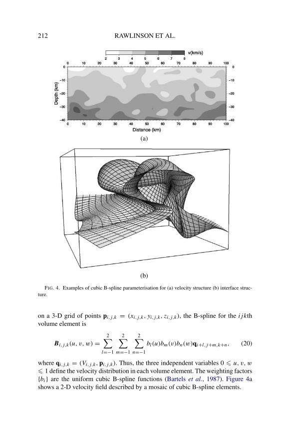
212 RAWLINSON ET AL.
(a)
(b)
FIG. 4. Examples of cubic B-spline parameterisation for (a) velocity structure (b) interface struc-ture.
on a 3-D grid of points pi,j,k = (xi,j,k, yi,j,k, zi,j,k), the B-spline for the ijkthvolume element is
(20)Bi,j,k(u, v,w) =2∑
l=−1
2∑m=−1
2∑n=−1
bl(u)bm(v)bn(w)qi+l,j+m,k+n,
where qi,j,k = (Vi,j,k, pi,j,k). Thus, the three independent variables 0 � u, v,w
� 1 define the velocity distribution in each volume element. The weighting factors{bi} are the uniform cubic B-spline functions (Bartels et al., 1987). Figure 4ashows a 2-D velocity field described by a mosaic of cubic B-spline elements.
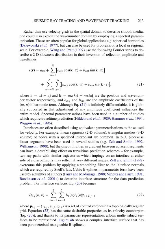
SEISMIC RAY TRACING AND WAVEFRONT TRACKING 213
Rather than use velocity grids in the spatial domain to describe smooth media,one could also exploit the wavenumber domain by employing a spectral parame-terisation. These are often popular for global applications e.g. spherical harmonics(Dziewonski et al., 1977), but can also be used for problems on a local or regionalscale. For example, Wang and Pratt (1997) use the following Fourier series to de-scribe a 2-D slowness distribution in their inversion of reflection amplitude andtraveltimes
s(r) = a00 +N∑
m=1
[am0 cos(k · r) + bm0 sin(k · r)
]
(21)+N∑
m=−N
N∑n=1
[amn cos(k · r) + bmn sin(k · r)
],
where r = xi + zj and k = mπk0i + nπk0j are the position and wavenum-ber vector respectively, and amn and bmn are the amplitude coefficients of the(m, n)th harmonic term. Although Eq. (21) is infinitely differentiable, it is glob-ally supported in that adjustment of any amplitude coefficient influences theentire model. Spectral parameterisations have been used in a number of studieswhich require traveltime prediction (Hildebrand et al., 1989; Hammer et al., 1994;Wiggins et al., 1996).
Interfaces are often described using equivalent parameterisations to those usedfor velocity. For example, linear segments (2-D volume), triangular meshes (3-Dvolume) or nodes with a specified interpolant are common. In 2-D, piecewiselinear segments have been used in several studies (e.g. Zelt and Smith, 1992;Williamson, 1990), but the discontinuities in gradient between adjacent segmentscan have a destabilising effect on traveltime prediction schemes – for example,two ray paths with similar trajectories which impinge on an interface at eitherside of a discontinuity may reflect at very different angles. Zelt and Smith (1992)overcome this problem by applying a smoothing filter to the interface normalswhich are required by Snell’s law. Cubic B-splines in parametric form have beenused by a number of authors (Farra and Madariaga, 1988; Virieux and Farra, 1991;Rawlinson et al., 2001a) to describe interface structure for the data predictionproblem. For interface surfaces, Eq. (20) becomes
(22)Bi,j (u, v) =2∑
k=−1
2∑l=−1
bk(u)bl(v)pi+k,j+l ,
where pi,j = (xi,j , yi,j , zi,j ) is a set of control vertices on a topologically regulargrid. Equation (22) has the same desirable properties as its velocity counterpart(Eq. (20)), and thanks to its parametric representation, allows multi-valued sur-faces to be represented. Figure 4b shows a complex interface surface that hasbeen parameterised using cubic B-splines.

214 RAWLINSON ET AL.
Finally, it is worth noting that irregular parameterisations have been used forboth ray based and grid based schemes. In the case of grid based schemes whichsolve the eikonal equation, irregular grids have the potential to improve compu-tational efficiency by varying grid resolution in response to wavefront curvature(e.g. Kimmel and Sethian, 1998; Qian and Symes, 2002). Another motivation foradopting irregular grids comes from seismic tomography; for many large seis-mic datasets, path distribution can be highly heterogeneous, resulting in a spatialvariability in resolving power. The ability to “tune” a parameterisation to thesevariations using some form of irregular mesh has a range of potential benefits,including increased computational efficiency (fewer unknowns), improved sta-bility of the inverse problem, and improved extraction of structural information(Michelini, 1995; Curtis and Snieder, 1997; Vesnaver et al., 2000; Spakman andBijwaard, 2001; Rawlinson and Sambridge, 2003a; Sambridge and Faletic, 2003;Sambridge et al., 2005). Completely unstructured meshes, such as those that useDelaunay tetrahedra or Voronoi polyhedra (Sambridge et al., 1995), offer highlevels of adaptability, but have special book-keeping requirements when solvingthe forward problem of data prediction. Sambridge et al. (1995) and Sambridgeand Gudmundsson (1998) describe techniques for locating points within thesemeshes, which allows ray tracing to be performed efficiently.
2. RAY TRACING SCHEMES
In this section, we describe a number of practical ray tracing schemes for solv-ing the boundary value problem of locating source-receiver ray paths in variousclasses of media (2-D, 3-D, with and without discontinuity). There are two broadcategories – shooting and bending – which exploit different formulations of theray tracing equations (Eq. (8)).
2.1. Shooting Methods
Shooting methods of ray tracing are conceptually simple; they formulate Eq. (8)as an initial value problem which allows a complete ray path (with appropriateapplication of Snell’s law in the presence of any interface) to be traced given aninitial trajectory of the path. The two point problem of finding a source-receiverpath then becomes an inverse problem in which the unknown is the initial di-rection vector of the ray, and the function to be minimised is a measure of thedistance between the ray end point and receiver. The main challenge that facesthis class of method is the non-linearity of the inverse problem, which tends toincrease dramatically with the complexity of the medium (as Fig. 1 testifies).

SEISMIC RAY TRACING AND WAVEFRONT TRACKING 215
2.1.1. The Initial Value Problem
The appropriate form of the equation required to solve the initial value problemdepends largely on the choice of parameterisation. In a medium described by con-stant velocity (slowness) blocks, the ray path is simply described by a piecewiseset of straight line segments; all that is required to solve the initial value problemis repeated application of Snell’s law at cell boundaries. This can be accomplishedwith high computational efficiency (e.g. Williamson, 1990). Analytic ray tracingcan also be applied to other parameterisations; for example, triangular or tetra-hedral meshes in which the velocity gradient is constant (e.g. White, 1989). Theexpression for ray trajectory in a medium with a constant velocity gradient can beexpressed in various ways, including parametrically as (Rawlinson et al., 2001a)
(23)x = v(z0)
k
[a0(c − c0)
1 − c20
,b0(c − c0)
1 − c20
, 1 −√
1 − c2
1 − c20
]+ x0,
where x0 is the origin of the ray segment, [a, b, c] is a unit vector tangent to theray path, [a0, b0, c0] is a unit vector tangent to the ray path at x0, k is the velocitygradient, and v(z0) is the velocity at z0. The associated traveltime is then givenby
(24)T = 1
2kln
[(1 + c
1 − c
)(1 − c0
1 + c0
)]+ T0,
where T0 is the traveltime from the source to x0. For application to tetrahedra (ortriangles in 2-D), it is simply a matter of rotating the coordinate system so thatthe velocity gradient is in the direction of the z-axis. A number of other velocityfunctions yield analytic ray tracing solutions, such as the constant gradient of ln v,and the constant gradient of the nth power of slowness 1/vn (Cervený, 2001).
Although analytic ray tracing is possible for a few special cases, in general oneneeds to solve Eq. (8) using numerical methods. This usually requires Eq. (8)to be reduced to a convenient first-order initial value system of equations, whichcan be done in a variety of ways. For example, by considering the following unitvector in the direction of the ray
(25)drdl
= [sin θ cos φ, sin θ sin φ, cos θ ],
where θ is the inclination of the ray with the vertical (z-axis), and φ is the azimuthof the ray (angle between ray and positive x-axis in xy plane). Substitution of thisexpression into Eq. (8) and application of the product rule yields:

216 RAWLINSON ET AL.
(26)
∂s
∂x= s cos θ cos φ
dθ
dl− s sin θ sin φ
dφ
dl+ sin θ cos φ
ds
dl
∂s
∂y= s cos θ sin φ
dθ
dl+ s sin θ cos φ
dφ
dl+ sin θ sin φ
ds
dl
∂s
∂z= −s sin θ
dθ
dl+ cos θ
ds
dl
⎫⎪⎪⎪⎪⎪⎪⎬⎪⎪⎪⎪⎪⎪⎭
.
These three equations can be rearranged to remove the ds/dl term and produceexpressions for dθ/dl and dφ/dl, which together with Eq. (25) produce the fol-lowing system of equations
(27)
dx
dl= sin θ cos φ
dy
dl= sin θ sin φ
dz
dl= cos θ
dθ
dl= cos θ
s
[cos φ
∂s
∂x+ sin φ
∂s
∂y
]− sin θ
s
∂s
∂z
dφ
dl= 1
s sin θ
[cos φ
∂s
∂y− sin φ
∂s
∂x
]
⎫⎪⎪⎪⎪⎪⎪⎪⎪⎪⎪⎪⎪⎪⎪⎪⎪⎪⎬⎪⎪⎪⎪⎪⎪⎪⎪⎪⎪⎪⎪⎪⎪⎪⎪⎪⎭
.
Thus, given some initial position and trajectory, a ray path can be obtained bysolving this coupled system of equations e.g. using a fourth order Runge–Kuttascheme (e.g. Kreyszig, 1993).
The initial value formulation of the kinematic ray tracing equations given byEq. (27) uses path length l as the independent variable. However, it is often moreconvenient to use traveltime t , since this parameter is usually required in additionto path geometry. Conversion of Eq. (27) into a form that uses t as the independentvariable and velocity v instead of slowness s (the use of slowness or velocity isoften a matter of convention, but it can have practical implications for certainclasses of problem, e.g. Rawlinson and Sambridge, 2003b) can be achieved usingthe following simple set of relationships
dθ
dl= s
dθ
dt,
(28)dφ
dl= s
dφ
dt,
dxdl
= sdxdt
,∂s
∂x= − 1
v2
∂v
∂x,

SEISMIC RAY TRACING AND WAVEFRONT TRACKING 217
FIG. 5. A fan of nine ray paths traced from a source point in a complex 2-D medium described bya mesh of cubic B-spline functions. A fourth order Runge–Kutta scheme is used to solve Eq. (29) inthis case.
which result in the following system of equations
(29)
dx
dt= v sin θ cos φ
dy
dt= v sin θ sin φ
dz
dt= v cos θ
dθ
dt= − cos θ
[cos φ
∂v
∂x+ sin φ
dv
dy
]− sin θ
∂v
∂z
dφ
dt= 1
sin θ
[sin φ
∂v
∂x− cos φ
∂v
∂y
]
⎫⎪⎪⎪⎪⎪⎪⎪⎪⎪⎪⎪⎪⎪⎪⎪⎪⎪⎬⎪⎪⎪⎪⎪⎪⎪⎪⎪⎪⎪⎪⎪⎪⎪⎪⎪⎭
.
This system of equations has a similar form to Eq. (27), and therefore can besolved using the same class of technique. The nine ray paths shown in Fig. 5were computed by solving Eq. (29) using a 4th order Runge–Kutta method (withconstant φ). This procedure is very efficient; for example, tracing 10,000 ray pathsusing a time step of 0.1 s from the same source point to the edge of the mediumonly takes 6 s on a 1.6 GHz Opteron PC running Linux.
Rather than use ray inclination and azimuth to describe ray trajectory, one couldalso use the components of the ray direction (or slowness) vector p = ∇T . Asystem of first-order equations can then be simply derived from Eq. (8) by usingthis vector as the substitution variable i.e. ∇T = s dr/dl. This results in

218 RAWLINSON ET AL.
(30)
drdl
= vp
dpdl
= ∇ 1
v
⎫⎪⎪⎬⎪⎪⎭ ,
which is a system of six equations. The independent variable s can be replaced bytraveltime t in the same way as before to produce
(31)
drdt
= v2p
dpdt
= −1
v∇v
⎫⎪⎪⎬⎪⎪⎭ .
This is the same set of equations that would result from substituting Eq. (11) intothe Hamilton equations (13). Although Eq. (29) has one less dependent variableto compute than Eq. (31), it contains trigonometric functions which, from a com-putational point of view, are less desirable. The 6D vector (r, p), which uniquelydescribes the position and trajectory of a ray in 3-D space, is sometimes referredto as the phase space vector (Chapman, 2004), while its 5-D counterpart (r, θ, φ)
is sometimes referred to as the reduced phase space vector (e.g. Osher et al.,2002).
It is worth emphasising that a variety of other first-order formulations of thekinematic ray tracing equations in isotropic media can be derived – for more de-tails, see Cervený (1987, 2001). In general anisotropic media, a system of sixfirst-order equations can be obtained by substituting the Hamiltonian defined byEq. (13) into the Hamilton equations, which results in (Cervený and Firbas, 1984;Chapman, 2004)
(32)
dxi
dt= ∂Gm
∂pi
= cijklpkgjmgl
m
ρ
dpi
dt= −∂Gm
∂xi
= −1
2
∂[cjklm/ρ]∂xi
pjpmgkmgl
m
⎫⎪⎪⎬⎪⎪⎭ .
Although much more computationally expensive to solve than its isotropic equiv-alent, initial value anisotropic ray tracing in 2-D or 3-D media does not pose asignificant challenge for modern computers.
In the presence of smooth velocity variations, the kinematic ray tracing equa-tions provide the required solution, but as soon as velocity discontinuities areintroduced, two additional problems need to be solved: (1) locate ray-interfaceintersection point; (2) find trajectory of departing ray path. The first problem canbe difficult to solve, particularly if both ray paths and interfaces are describedby non-linear functions. If a medium is divided up into cells, then a first level ofrefinement can be achieved by simply knowing which cells contain an interface;

SEISMIC RAY TRACING AND WAVEFRONT TRACKING 219
FIG. 6. Reflection paths from two source points in the presence of a complex multi-valued inter-face described by cubic B-splines. Path trajectories are obtained by solving an initial value problemuntil the ray impinges on the surface z = 0. Note that it is decided a priori that all rays impinging onthe interface will reflect. Thus, rays trapped inside complex features of the model keep reflecting untilthey finally emerge and intersect with the surface.
thus when a ray enters a cell, one knows whether or not an intersection is possi-ble. Sambridge and Kennett (1990) devise a boundary value ray tracing schemefor 3-D media which contain discontinuities; rather than exactly locate the ray-interface intersection point, the time step length used in Eq. (29) is iterativelyadjusted in the vicinity of an interface based on a linear update procedure. The it-eration process ceases when the distance between the ray end point and interfacesatisfies a tolerance criteria.
In an alternative approach, Virieux and Farra (1991) exploit the convex hull andsubdivision properties of B-splines. The first property states that the B-spline sur-face must lie within the convex volume defined by the control points; the secondproperty allows the same surface to be described by larger numbers of controlpoints. Thus, the approximate location of a ray-interface intersection point canbe found by determining whether the ray (locally linear in this case) intersects aparallelepiped containing the convex volume; if it does, then the convex volumecan be subdivided and the simple ray-parallelepiped problem can be resolved foreach of the new, smaller, parallelepipeds. Repetition of this process allows allpossible intersection points to be found. This scheme is very robust, but can becomputationally expensive; as a result, Virieux and Farra (1991) switch to a moreefficient local search method once it is considered a unique intersection point isbeing targeted by the subdivision scheme.
Like Virieux and Farra (1991), Rawlinson et al. (2001a) also use cubic B-splines in parametric form to represent interface surfaces, but adopt a differentapproach to finding ray-interface intersection points. In this case, rays are de-

220 RAWLINSON ET AL.
fined by circular arc segments. Rather than exploit the convex hull property ofB-splines, an initial intersection point is found by approximating the surface bya mosaic of triangular patches, for which analytic solution of the ray-interfaceintersection problem is possible. Once a preliminary intersection point is found,an iterative non-linear scheme based on the generalised Newton method is usedto target the true intersection point. Although computationally efficient, the pro-cedure may fail to locate some intersection points, particularly if the trajectoryof the ray is nearly parallel to the interface when intersection occurs. Anotherpossible problem is that the local method converges to the incorrect intersectionpoint. However, in practice the scheme is effective, as demonstrated in 2-D byFig. 6, which shows reflection paths propagating through a highly complex inter-face structure. As well as demonstrating the robustness of the intersection scheme,this example also illustrates the power of initial value ray tracing: given virtuallyany structure, it is possible to trace ray paths of almost any specified initial trajec-tory.
The second problem that needs to be solved when a ray impinges on aninterface is to find the trajectory of the departing ray path. In 2-D, a sim-ple application of Snell’s law (Eq. (10)) can produce up to four departingpaths (transmission, reflection, converted transmission, converted reflection) forisotropic media. In 3-D, the same class of paths can be generated, but in addi-tion to Snell’s law, the continuity of projection of the incident ray must alsobe considered. This is equivalent to requiring that the incident path, depart-ing path and normal to the interface at the intersection point, all lie in thesame plane. By combining this constraint with Snell’s law, the slowness vec-tor pr of the reflected or refracted ray path can be defined by (Cervený, 1987;Sambridge and Kennett, 1990):
(33)pr = pi +{κ
[1
v2r
− 1
v2i
+ (pi · n)2]1/2
− pi · n}
n,
where pi is the slowness vector of the incident path, n is a normal vector to theinterface at the intersection point, and vi and vr are the wavespeeds of the incidentand departing rays. κ = sign(pi ·n) and equals +1 if pi makes an acute angle withn and −1 otherwise. When unconverted reflected waves are required (vi = vr ),Eq. (33) reduces to:
(34)pr = pi − 2(pi · n)n.
For general anisotropic media, up to three reflected and three transmitted wavescan be generated for a single incident path – see Slawinski et al. (2000) for detailson how they can be calculated.

SEISMIC RAY TRACING AND WAVEFRONT TRACKING 221
FIG. 7. Principle of the shooting method. In this case, an initial path trajectory is updated until itconverges at the receiver.
2.1.2. The Boundary Value Problem
Shooting methods of ray tracing usually solve the boundary value problem byprobing the medium with initial value ray paths and then exploiting informationfrom the computed paths to better target the receiver. Figure 7 illustrates this basicconcept in 2-D. If a ray emanates from a source point in a 3-D medium with takeoff angles θo and φo, and the aim is for the ray end point (xe, ye) on the receiverplane (z = constant) to coincide with the receiver location (Xr, Yr), then theboundary value problem amounts to finding the (θo, φo) that solve the two non-linear simultaneous equations
(35)xe(θo, φo) = Xr
ye(θo, φo) = Yr
}.
Given that (xe, ye) cannot be expressed explicitly as a function of (θo, φo) formost velocity fields, it is usually the case that the boundary value problem is posedas an optimisation problem, with the misfit function to be minimised expressed assome measure of the distance between the ray end point and its intended target.Since the optimisation problem is non-linear, a range of iterative non-linear andfully non-linear schemes can be applied.
Julian and Gubbins (1977) propose two iterative non-linear schemes for solv-ing Eq. (35). The first of these is Newton’s method, which amounts to a simplelinearisation:
(36)
⎡⎢⎣
∂xe
∂θo
∂xe
∂φo
∂ye
∂θo
∂ye
∂φo
⎤⎥⎦[
θn+1o − θn
o
φn+1o − φn
o
]=[
Xr − xe(θno , φn
o )
Yr − ye(θno , φn
o )
].

222 RAWLINSON ET AL.
(a)
(b)
FIG. 8. Two-point paths computed through a 3-D layered model using the shooting scheme ofRawlinson et al. (2001a). (a) Refracted paths, (b) reflected paths.
Thus, given some starting initial trajectory θ0o , φ0
o , solution of Eq. (36) provides anupdated initial trajectory θ1
o , φ1o , and the process is repeated until an appropriate
tolerance criterion is met. The success of this scheme depends largely on two fac-tors: (1) accurate calculation of the partial derivative matrix, and (2) obtaining aninitial guess ray that will converge to the correct minimum under the assumptionof local linearity. Both of these requirements can be difficult to satisfy, particularlyin complex media. One approach to estimating the partial derivatives involves fit-ting two planes through the end points of a cluster of three ray paths with differentinitial projection angles (i.e. one plane through all three xo(θo, φo) and the otherplane through all three yo(θo, φo)). The gradient of these planes in the θo and φo
directions provide estimates of the four partial derivatives in Eq. (36). This ap-proach is actually equivalent to the method of false position, which is the seconditerative non-linear scheme proposed by Julian and Gubbins (1977). The methodof false position is unlikely to be first-order accurate like a true Newton method,and therefore will converge more slowly and possibly with less stability. How-ever, it will be faster at each iteration, and Rawlinson et al. (2001a, 2001b) foundit to be sufficiently robust to use in solving the forward step of large 3-D tomo-graphic inverse problems. Figure 8 shows two-point paths through a 3-D laterallyheterogeneous structure that were computed using this scheme.
Sambridge and Kennett (1990) directly compute the partial derivatives inEq. (36) by exploiting wavefront curvature information at the end point of the ray.This can be done by differentiating Eq. (29) with respect to the initial take-off an-
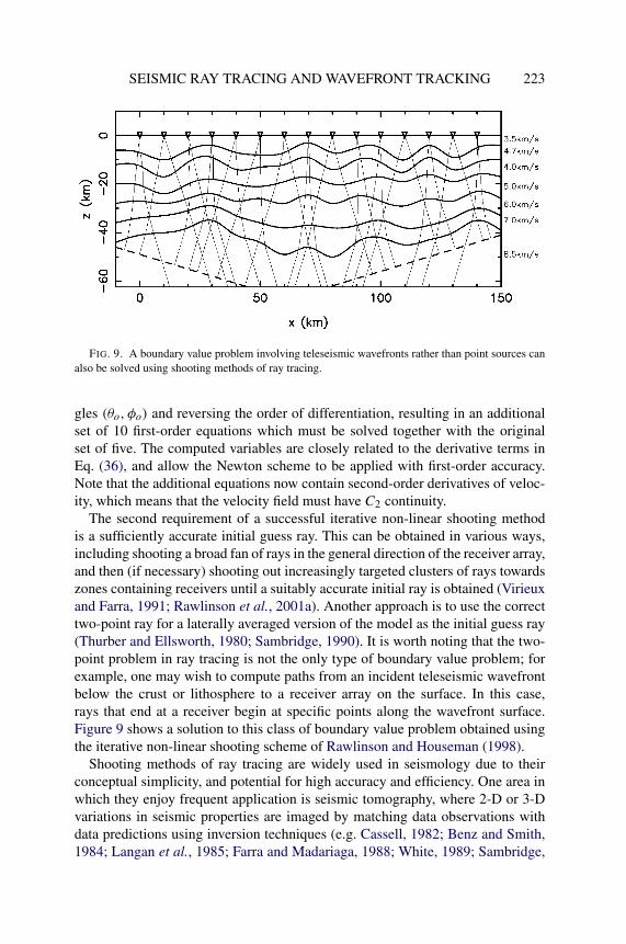
SEISMIC RAY TRACING AND WAVEFRONT TRACKING 223
FIG. 9. A boundary value problem involving teleseismic wavefronts rather than point sources canalso be solved using shooting methods of ray tracing.
gles (θo, φo) and reversing the order of differentiation, resulting in an additionalset of 10 first-order equations which must be solved together with the originalset of five. The computed variables are closely related to the derivative terms inEq. (36), and allow the Newton scheme to be applied with first-order accuracy.Note that the additional equations now contain second-order derivatives of veloc-ity, which means that the velocity field must have C2 continuity.
The second requirement of a successful iterative non-linear shooting methodis a sufficiently accurate initial guess ray. This can be obtained in various ways,including shooting a broad fan of rays in the general direction of the receiver array,and then (if necessary) shooting out increasingly targeted clusters of rays towardszones containing receivers until a suitably accurate initial ray is obtained (Virieuxand Farra, 1991; Rawlinson et al., 2001a). Another approach is to use the correcttwo-point ray for a laterally averaged version of the model as the initial guess ray(Thurber and Ellsworth, 1980; Sambridge, 1990). It is worth noting that the two-point problem in ray tracing is not the only type of boundary value problem; forexample, one may wish to compute paths from an incident teleseismic wavefrontbelow the crust or lithosphere to a receiver array on the surface. In this case,rays that end at a receiver begin at specific points along the wavefront surface.Figure 9 shows a solution to this class of boundary value problem obtained usingthe iterative non-linear shooting scheme of Rawlinson and Houseman (1998).
Shooting methods of ray tracing are widely used in seismology due to theirconceptual simplicity, and potential for high accuracy and efficiency. One area inwhich they enjoy frequent application is seismic tomography, where 2-D or 3-Dvariations in seismic properties are imaged by matching data observations withdata predictions using inversion techniques (e.g. Cassell, 1982; Benz and Smith,1984; Langan et al., 1985; Farra and Madariaga, 1988; White, 1989; Sambridge,

224 RAWLINSON ET AL.
1990; Zelt and Smith, 1992; VanDecar et al., 1995; McCaughey and Singh, 1997;Rawlinson et al., 2001b).
2.1.3. Paraxial Ray Tracing
An important field of ray theory that is yet to be mentioned is the parax-ial ray approximation (Cervený and Pšencik, 1983; Cervený and Firbas, 1984;Cervený, 1987; Farra and Madariaga, 1988; Virieux and Farra, 1991; Cervený,2001; Cervený et al., 2006), which is widely employed by the seismology com-munity for various aspects of data prediction. It essentially involves using firstorder perturbation theory to deduce characteristics of the wavefield in the neigh-bourhood of a reference ray. Thus, given some reference path with position andslowness vector y0(t) = [r0(t), p0(t)]T, a paraxial ray can be defined by the first-order approximation
(37)y(t) = y0(t) + δy(t) = [r0(t) + δx(t), p0(t) + δp(t)
].
To obtain the paraxial ray tracing equations, consider the linearisation of the kine-matic ray tracing equations r = ∇pH and p = −∇rH (equivalent to Eq. (13) with( ˙ ) denoting differentiation with respect to t), which can be written as
(38)δr = ∂ r
∂rδr + ∂ r
∂pδp
δp = ∂p∂r
δr + ∂p∂p
δp
⎫⎪⎪⎬⎪⎪⎭ ,
or in more compact form as
(39)δy = Aδy where A =[ ∇r∇pH ∇p∇pH
−∇r∇rH −∇p∇rH
].
The paraxial ray tracing equation has six independent solutions in 3-D and fourin 2-D. Since we can write that
(40)y(t) = y(t0) + dy(t)
dtδt = y(t0) + ∂y(t)
∂y(t0)
dy(t0)
dtδt,
it is common to express the solution to Eq. (39) in terms of a ray propagator matrixP(t, t0) (see Cervený, 1987; Virieux and Farra, 1991)
(41)δy(t) = P(t, t0)δy(t0) where P(t, t0) =⎡⎢⎣
∂x(t)
∂x(t0)
∂x(t)
∂p(t0)
∂p(t)
∂x(t0)
∂p(t)
∂p(t0)
⎤⎥⎦ ,
which has the initial condition that P(t = t0, t0) = I , the identity matrix. Thepower of paraxial rays is that they allow information about the wavefield in thevicinity of a reference ray to be used, for example to detect caustics in two-point ray tracing. In fact, the shooting method of Sambridge and Kennett (1990)

SEISMIC RAY TRACING AND WAVEFRONT TRACKING 225
described in the previous section, which makes use of wavefront curvature in-formation in the vicinity of a ray to compute partial derivatives for an iterativenon-linear update scheme, is an example of using paraxial ray theory in two-point ray tracing. Virieux and Farra (1991) describe a similar scheme, and infact there are many shooting schemes of ray tracing which exploit the paraxialray approximation (e.g. Cervený and Firbas, 1984; Farra and Madariaga, 1988;Bulant, 1996). For more details on paraxial ray theory and its many other po-tential applications, refer to Cervený and Pšencik (1983); Cervený and Firbas(1984); Cervený et al. (1984); Cervený (1987); Farra and Madariaga (1987);Klimeš (1989); Bulant (1996); Cervený (2001); Cervený et al. (2006).
2.1.4. Fully Non-Linear Shooting Methods
Shooting methods which use an iterative non-linear approach to solve theboundary value problem are often very efficient in mildly heterogeneous media,but generally become less robust as the complexity of the medium increases. Fig-ure 10 illustrates why this is the case by showing the relationship between rayinclination angle and distance from a receiver for two velocity models of differentcomplexity. In the first model (Fig. 10a), velocity increases linearly with depthbut has random velocity fluctuations with a standard deviation of 0.4 km/s super-imposed. These velocity perturbations are sufficient to cause some mild focusingand defocusing of the wavefront, as reflected by the variable density of ray pathsalong the surface. This effect is also manifest in the corresponding plot of rayend point to receiver distance vs. initial ray inclination; the plot is asymmetricalabout 0◦ (vertical initial inclination) and contains significant variations in curva-ture. Despite these non-linearities, it is likely that any iterative non-linear shootingscheme will converge to the correct solution using a starting ray with initial anglein the range −45◦ → 45◦, although the initiation of a triplication several kilome-tres to the right of the receiver (Fig. 10a) may cause some difficulties (it appearsas a small region of near zero gradient in the ray inclination vs. distance plot atabout −4◦).
The second model (Fig. 10b) is identical to Fig. 10a except that the randomvelocity fluctuations now have a standard deviation of 1.4 km/s, which results insignificant lateral heterogeneity. Note that the pattern of anomalies is identical tothe first model; it is only their amplitude which has changed. The effect of theincreased amplitude on the ray distribution is dramatic, with several triplicationsof the ray field now evident. The corresponding distance vs. ray inclination plotreveal these multi-pathing effects as extrema. Clearly, at least three arrivals aredetected by the receiver. If one was to use an iterative non-linear shooting methodin this situation with a starting ray in the initial inclination range of −45◦ → 45◦,then it is possible that a two point path will be located, but it is also possible thatthe scheme will become trapped in a local minimum. Shooting a broad fan ofrays, and then increasingly more targeted clusters based on previous sampling of

226 RAWLINSON ET AL.
(a)
(b)
FIG. 10. Demonstration of the non-linear relationship that exists between initial ray trajectoryand distance from ray end point to receiver. (a) Mildly heterogeneous medium with lateral velocitystandard deviation of 0.4 km/s; (b) strongly heterogeneous medium with lateral velocity standarddeviation of 1.4 km/s. The source is denoted by a grey circle and the receiver by a grey triangle. Notethat while 100 ray paths are shown in each of the ray tracing plots (top), the corresponding ray endpoint vs. initial ray inclination diagrams (bottom) were generated using 1,000 rays.

SEISMIC RAY TRACING AND WAVEFRONT TRACKING 227
the wavefield, may provide sufficiently accurate initial rays (e.g. Rawlinson et al.,2001a) to locate one or more global minima. Ultimately, though, there will be atrade-off between computing time and the number of two-point paths found, andone must always make a decision as to which point along this trade-off curve isadequate for the problem at hand.
Given the potential pitfalls of using an iterative non-linear solver in two pointshooting methods, it would appear that fully non-linear solvers would be at leastworthy of investigation. However, there are relatively few examples in the litera-ture, perhaps due to the recent proliferation of grid based and wavefront construc-tion type schemes that are designed to overcome these limitations (these schemeswill be discussed later in some detail). Velis and Ulrych (1996) describe a fullynon-linear shooting method of ray tracing that uses simulated annealing to locatethe global minimum path. Simulated annealing (e.g. Kirkpatrick et al., 1983) isbased on an analogy with physical annealing in thermodynamic systems to guidevariations to the model parameters, in this case the initial ray trajectories. Velisand Ulrych (2001) extend their method to heterogeneous 3-D velocity modelswhich can include variable thickness layers, faults, and complex structures suchas salt domes. The scheme exhibits several advantages compared to more con-ventional ray tracing schemes; in particular increased robustness for locating theglobal minimum solution. However, it does not appear to be practical for find-ing all multipaths, and tends to be more computationally expensive than iterativenon-linear solvers.
2.2. Bending Methods
The principle of the bending method of ray tracing is to iteratively adjust thegeometry of an initial arbitrary path that joins source and receiver until it becomesa true ray path (i.e. it satisfies Fermat’s principle of stationary time) – see Fig. 11.A common approach to implementing the bending method is to derive a boundaryvalue formulation of the kinematic ray tracing equations which can then be solvediteratively. There are many ways that this can be done; here, we describe a schemethat was first devised by Julian and Gubbins (1977). The traveltime T of a ray pathbetween source S and receiver R can in general be expressed by the integral
(42)T =∫ R
S
s dl,
where s is slowness and l is path length. The ray path can be described paramet-rically by a monotonic function λ, the normalised path length (λ = l/L, where L
is the total path length of the ray), in which case r = r(λ). A perturbation in pathlength can therefore be written as
(43)dl
dλ= √
r · r =√
x2 + y2 + z2 = F,

228 RAWLINSON ET AL.
FIG. 11. Principle of the bending method. In this case, an initial two point path is perturbed untilit satisfies Fermat’s principle.
where ( ˙ ) denotes differentiation with respect to λ, and the use of normalised pathlength means that F = L and dF/dλ = 0. Using this expression, Eq. (42) can berewritten as
(44)T =∫ R
S
sF dλ.
The ray tracing equations can be obtained by extremizing this integral usingthe calculus of variations (e.g. Jeffreys and Swirles, 1966). For any integrandG(λ, r(λ), r(λ)) the Euler–Lagrange equations are
(45)∂G
∂r− d
dλ
[∂G
∂ r
]= 0.
In our case, the integrand is G = sF = s√
r · r, and substitution into Eq. (45)yields
(46)sr + (r · ∇s)r − (r · r)∇s = 0.
It is easy to show that only two of these equations are independent (Julian andGubbins, 1977), and that one may be ignored without loss of generality. Thisleaves two equations with three unknowns r = (x, y, z); a final constraint comesfrom dF/dλ = 0 (so (r · r) = 0). Thus, a system of three independent non-linearsecond-order differential equations can be explicitly written (Julian and Gubbins,1977)
(47)
sx + syyx + szzx − sx(y2 + z2
) = 0
sy + sxxy + szzy − sy(x2 + z2
) = 0
xx + yy + zz = 0
⎫⎪⎪⎪⎬⎪⎪⎪⎭
,

SEISMIC RAY TRACING AND WAVEFRONT TRACKING 229
where ∇s = (sx, sy, sz). The boundary conditions for this problem are r(0) = rS
and r(1) = rR , and an iterative non-linear solution approach is possible givensome initial estimate of the path r(λ)0, so that in general r(λ)n+1 = r(λ)n +δr(λ)n. Substitution of this expression into Eq. (47) and linearising the resultingequations for δr(λ)n allows solutions to be obtained using, for example, sec-ond order finite difference techniques (Julian and Gubbins, 1977). The iterativeprocess can be continued until some suitable convergence criterion, based on thepath perturbation integrated along the ray, is satisfied.
Pereyra et al. (1980) devise a similar technique to that described above for raybending, but extend it to allow for the presence of interfaces. This can be achievedby considering a separate system of differential equations in each smooth region,and coupling them using the known discontinuity condition at each interface thatis traversed by the ray path. The order in which the interfaces are intersectedby the ray path needs to be known in advance, which may be a drawback incomplex structures. This scheme is developed further in very complex 3-D modelsby Pereyra (1996), who also implements shooting to obtain an initial guess ray.This helps to overcome the problem of knowing a priori the correct path sequence.
2.2.1. Pseudo-Bending Methods
Pseudo-bending methods are similar in principle to the bending scheme de-scribed above, but avoid direct solution of the ray equations. One of the first ofthese schemes was developed by Um and Thurber (1987), and is based upon theray path being represented by a set of linearly interpolated points. Given someinitial arbitrary path, the aim is to sequentially adjust the location of each pointso that the path better satisfies the ray equations. This can be accomplished quiteefficiently by locating the direction of the ray path normal and then directly ex-ploiting Fermat’s principle of stationary time. If we denote mt and mn as vectorstangent and normal to the ray path respectively at some point r (see Fig. 12a),then
(48)mt = drdl
and mn = dmt
dl,
where mt is a unit vector. By using Eq. (5), mn can be written
(49)mn = d
dl
(∇T
s
)= 1
s
d∇T
dl+ s∇T
d
dl
(1
s
).
mn can be expressed completely in terms of s and mt by making use of Eq. (7),so that
(50)mn = ∇s
s+ ∇T
d
dr
(1
s
)· dr
dl= 1
s
(∇s − (∇s · mt )mt
).

230 RAWLINSON ET AL.
(a) (b)
FIG. 12. Schematic representation of parameters used in the pseudo bending method. (a) Defin-ition of ray tangent mt , ray normal mn and antinormal unit vector n at a point r along a ray path;(b) stencil for the three point perturbation scheme.
If we now let n represent the anti-normal unit vector to the ray path at r, andsubstitute velocity v for slowness s, then
(51)n = ∇v − (∇v · mt )mt
|∇v − (∇v · mt )mt |which is equivalent to the expression derived by Um and Thurber (1987). Thevector n thus defines the direction of ray path curvature.
A three-point perturbation scheme is devised by Um and Thurber (1987) tosequentially update points along a path. Consider Fig. 12b, which shows threepoints ri−1, ri and ri+1. The aim is to replace the initial guess point rold
i withan improved estimate rnew
i . The improved estimate is obtained by considering aperturbation to the point rmid, which lies at the midpoint between ri−1 and ri+1.The vector mt can then be simply approximated by
(52)mt = ri+1 − ri−1
|ri+1 − ri−1|and the anti-normal unit vector n, which specifies the bending direction, is com-puted from Eq. (51). The next step is to find the distance R in the direction nwhich results in an improved estimate of the path. An approximate analytic ex-pression for the traveltime T (R) between ri−1 and ri+1 can be obtained using thetrapezoidal rule
(53)T (R) =√
L2 + R2
[1
vnewi
+ 1
2
(1
vi−1+ 1
vi+1
)].
The appropriate value for R can be obtained by appealing directly to Fermat’sprinciple of stationary time, which in this case equates to setting dT/dR = 0.

SEISMIC RAY TRACING AND WAVEFRONT TRACKING 231
Therefore,
(54)
dT
dR= √
L2 + R2 d
dR
(1
vnewi
)+(
1
vnewi
+ c
)R√
L2 + R2
= (L2 + R2
)dvnewi
dR− Rvnew
i
(cvnew
i + 1) = 0
⎫⎪⎪⎬⎪⎪⎭ ,
where c = (1/vi−1 + 1/vi+1)/2. The quantity vnewi is unknown, but a first-order
accurate (in R) estimate based on the velocity and velocity gradient at rmid can bemade
(55)vnewi ≈ vmid + (n · ∇vmid)R.
Substitution of this expression into Eq. (54) results in[c(n · ∇vmid)
2]R3 − [2cvmid(n · ∇vmid)
]R2 − [
vmid(cvmid + 1)]R
(56)+ (n · ∇vmid)L2 = 0.
Um and Thurber (1987) ignore the cubic term of R, which results in a quadraticequation with two roots. The solution which produces real positive traveltimes is
(57)
R =−vmid(cvmid + 1) +
√v2
mid(cvmid + 1)2 + 8cvmid(n · ∇vmid)2L2
4cvmid(n · ∇vmid).
The update procedure for pseudo bending as outlined above is very simple andcomputationally efficient, as it only requires two relatively simply equations to besolved (Eqs. (51) and (57)). In practice, Um and Thurber (1987) apply the updatescheme simultaneously from both end points of the ray path to the central point.This process is repeated until a convergence criterion is met. An initial path canbe approximated in various ways, but one simple option is to begin with a threepoint ray joining source and receiver. Once the central point has been perturbed,two new points are introduced that bisect each line segment. The central threepoints can then be relocated, before four new points are introduced in the sameway as before (see Fig. 13). This process can be continued until a suitably accuratepath is obtained.
Despite the relatively crude approximations made in pseudo bending, Um andThurber (1987) find it to be much more computationally efficient than conven-tional bending schemes; consequently, it has become quite popular for problemswhich require large traveltime datasets to be predicted, e.g. 3-D local earthquaketomography (Eberhart-Phillips, 1990; Scott et al., 1994; Eberhart-Phillips andReyners, 1997; Graeber and Asch, 1999). Zhao et al. (1992) modify the threepoint perturbation scheme of Um and Thurber (1987) to allow for the presence ofinterfaces. In this case, the sequence of points which discretely defines the pathincludes points which lie on each interface traversed by the ray. When the update

232 RAWLINSON ET AL.
FIG. 13. Principle of the pseudo-bending method of Um and Thurber (1987). In this schematicexample, an initial guess ray is defined by three points. The center point is perturbed to satisfy Fermat’sprinciple of stationary time. The number of path segments is then doubled and the process repeated.
scheme reaches these points, they are perturbed along the interface (with adja-cent points on either side of the interface held fixed) until Snell’s law is satisfied.Koketsu and Sekine (1998) devise a similar scheme in a 3-D spherical coordinatesystem.
2.2.2. Other Bending Schemes
Two classes of bending method have been described above. In the first, the rayequation is linearised and iteratively solved as a boundary value problem withfixed end points. The second approach – pseudo bending – applies a simple per-turbation scheme based on a direct application of Fermat’s principle of stationarytime, to a ray path described by a sequence of points. Although these are the twoprincipal methods, several other schemes have been developed which warrant abrief mention.
Prothero et al. (1988) develop a 3-D bending scheme based on the simplexmethod of function minimisation. An initial path is obtained by using an exhaus-tive search method to find the minimum-time circular path between source andreceiver. Perturbations to this path, described by a sum of sine-wave harmonics,are then made using the simplex method, which searches for the amplitude co-efficients that produce the path of least time. Although the method appears to bemore robust than pseudo-bending, it is significantly slower.
Like ray shooting, ray bending can also be carried out using fully non-linearupdate schemes. Sadeghi et al. (1999) develop a method which uses genetic al-gorithms (GAs) to globally search for the minimum time ray path between twofixed points. The scheme is similar to pseudo-bending in that paths are describedby a set of linearly interpolated points, which are perturbed until a convergencecriterion is satisfied. However, in this case, a population of multiple two-point

SEISMIC RAY TRACING AND WAVEFRONT TRACKING 233
paths join source and receiver, and the GA drives the bending of paths until thetraveltime converges to a minimum. When this occurs, all two point rays withinthe population should follow almost identical paths.
Debski and Ando (2004) develop a so-called “spectral ray tracer”, which baressome resemblance to the scheme of Prothero et al. (1988), except that ray pathsare parameterised as a series of Chebyshev polynomials. The bending problemcan then be formulated as one of function minimisation, in which the decom-position coefficients of the Chebyshev polynomials become the variables to beadjusted until the two point traveltime is minimised. Instead of adopting a lin-earised approach to the optimisation problem, Debski and Ando (2004) use agenetic algorithm to generate and select the decomposition components.
Most schemes for solving the boundary value problem in ray tracing can usu-ally be characterised as either shooting or bending. However, other schemes do ex-ist, most notably those that are based on structural perturbation (Cervený, 2001).In this type of scheme, a known two point path exists in a reference medium,and the aim is to locate the equivalent two point path in a medium that is slightlymodified from the reference medium. Solution of this class of problem can beachieved using ray perturbation theory, which is described in various papers in-cluding Farra and Madariaga (1987); Snieder and Sambridge (1992); Pulliam andSnieder (1996). Snieder and Spencer (1993) show that ray bending and ray per-turbation theories can in fact be combined into a single perturbation theory.
3. GRID BASED SCHEMES
An alternative to tracing rays between source and receiver is to compute thetraveltime of the evolving wavefront at all points of a grid which spans themedium. The complete traveltime field implicitly contains the wavefront locationas a function of time (i.e. isochrons of T (x)) and all possible ray path trajectories(specified by ∇T ). Compared to conventional shooting and bending methods ofray tracing (Julian and Gubbins, 1977; Cassell, 1982; Um and Thurber, 1987;Virieux and Farra, 1991; Koketsu and Sekine, 1998), grid based traveltimeschemes have a number of clear advantages: (1) Most are capable of computingtraveltimes to all points of a medium, and will locate diffractions in ray shadowzones; (2) the non-linearity of both ray shooting and bending means that theymay fail to converge to a true two-point path, whereas most grid based schemesare highly stable and will find the correct solution even in strongly heterogeneousmedia; (3) grid based schemes can be very efficient in computing traveltime andpath information to the level of accuracy required by practical problems. Raytracing schemes can be inefficient if solution non-linearity is significant; (4) mostgrid-based schemes consistently find first-arrivals in continuous media. It is oftendifficult to ascertain with ray tracing whether the located path is a first or laterarrival.

234 RAWLINSON ET AL.
Despite these advantages, grid based schemes have a number of limitationswhich should be considered prior to application. These include: (1) accuracy isa function of grid spacing – in 3-D halving the spacing of a grid will increasecomputation time by at least a factor of 8. Thus, computation time may be-come unacceptable if highly accurate traveltimes are required; (2) most practicalschemes compute first-arrivals only – thus, features such as wavefront triplica-tions cannot be predicted; (3) quantities other than traveltime (such as amplitude)are difficult to compute accurately without first extracting path geometry and ap-plying ray based techniques. Two grid-based schemes – finite difference solutionof the eikonal equation and shortest path methods – have emerged in the last fewdecades as popular alternatives to conventional ray tracing, and are described be-low.
3.1. Eikonal Solvers
One of the first grid schemes based on finite difference solution of the eikonalequation was proposed by Vidale (1988). From a given source point, travel-times are progressively computed outwards along an expanding square in 2-D(see Fig. 14). Traveltimes to points which lie in the initial square around thesource point are computed as follows. The four points (i ± 1, j) and (i, j ± 1)
have traveltimes estimated by the formulae Ti±1,j = δx/2(si±1,j + si,j ) andTi,j±1 = δz/2(si,j±1 + si,j ), where s is slowness and δx and δz are grid spacingin x and z. The remaining four points are computed by appealing to the eikonalequation (Eq. (3)); in particular, the ∇T term can be approximated in the cell
FIG. 14. The expanding square method for progressive calculation of traveltimes throughout agridded velocity field.

SEISMIC RAY TRACING AND WAVEFRONT TRACKING 235
defined by points (i, j), (i + 1, j), (i, j + 1) and (i + 1, j + 1) by
(58)
∂T
∂x= Ti,j + Ti,j+1 − Ti+1,j − Ti+1,j+1
2δx
∂T
∂z= Ti,j + Ti+1,j − Ti,j+1 − Ti+1,j+1
2δz
⎫⎪⎪⎬⎪⎪⎭ .
Substitution into Eq. (3) produces the following quadratic equation
(Ti,j + Ti,j+1 − Ti+1,j − Ti+1,j+1)2
δx2
(59)+ (Ti,j + Ti+1,j − Ti,j+1 − Ti+1,j+1)2
δz2= 4s2,
where s is the average slowness of all four points defining the cell. This equationcan easily be solved for Ti+1,j+1. If h = δx = δz (Vidale, 1988), then the solution
to Eq. (59) has the simple form Ti+1,j+1 = Ti,j +√
2(hs)2 − (Ti,j+1 − Ti+1,j )2.Vidale (1988) also defines a solution stencil for a locally circular wavefront. Thisallows a mixed scheme to be devised, which uses the locally circular assumptionin regions of high wavefront curvature (e.g. in the source neighbourhood), andEq. (59) when the wavefront is more planar.
As the computational front evolves outward from the source, points within thesquare band cannot have traveltimes computed in arbitrary order; causality at leastrequires that new traveltimes be computed using only those traveltimes from sur-rounding points of lesser value. Vidale (1988) devises a scheme which sweepsthrough each of the four sides of the square in order to locate the minimum timesolution at each point. The resulting computational scheme is both fast and ac-curate, with CPU time being approximately proportional to the number of pointsdefining the grid. The method is readily extendable to 3-D, as demonstrated byVidale (1990).
The use of an expanding square formalism to define the shape of the computa-tional front cannot always respect the direction of flow of traveltime informationthrough the medium. This is demonstrated in Fig. 15, which shows how the ex-panding square can fail if the first-arriving path to a point inside the square needsto sample structure outside the square. As a consequence, first-arrivals are notalways guaranteed, which can ultimately lead to instability. Nevertheless, the ba-sic scheme proposed by Vidale (1988) remains popular, and its stability has beenimproved upon by introducing new features to the finite difference stencil andevolution of the computational front. Both Hole and Zelt (1995) and Afnimar andKoketsu (2000) introduce special headwave operators to better deal with the pres-ence of strong velocity contrasts, and Hole and Zelt (1995) implement an iterativepost-sweeping scheme to help account for the non-causal nature of the expand-ing square. van Trier and Symes (1991) use entropy-satisfying first-order upwind

236 RAWLINSON ET AL.
FIG. 15. Schematic illustration of how the expanding square method can fail. In this example,path 1 would be computed by the expanding square, but path 2 actually arrives first.
difference operators to improve the computational efficiency of the method andbetter deal with wavefront discontinuities. Comparable improvements are madeby Podvin and Lecomte (1991), who systematically apply Huygen’s principle inthe finite difference approximation in order to account for all possible modes ofpropagation.
More recently, Essentially Non-Oscillatory (ENO) finite difference schemesdeveloped in the field of computational mathematics (Shu and Osher, 1988, 1989)have been used to solve the eikonal equation within an expanding square frame-work. The attraction of ENO schemes is that they can be readily extended tovery high orders of accuracy, yet remain stable. Kim and Cook (1999) present ascheme, which they describe as ENO-DNO-PS, to efficiently compute first-arrivaltraveltime fields. DNO (or down ‘n’ out) refers to the expanding box scheme firstintroduced by Vidale (1988), and PS refers to post-sweeping, which is an iterativecorrection strategy applied to the traveltime field computed by ENO-DNO in anattempt to deal with causality breaches introduced by the expanding box. Thiscorrection scheme is similar in principle to the one used by Hole and Zelt (1995).Fig. 16 demonstrates the importance of post-sweeping in complex models; theexpanding box results in the overestimation of traveltimes in various regions ofthe model (dashed lines), which appear to be corrected by the post-sweeping step(solid line). A third-order WENO-DNO-PS solver is used in this example, whichis slightly different to that used by Kim and Cook (1999). Weighted EssentiallyNon-Oscillatory or WENO schemes have a number of advantages over ENO in-

SEISMIC RAY TRACING AND WAVEFRONT TRACKING 237
FIG. 16. Illustration of how post-sweeping can correct for errors due to the use of an expand-ing box strategy for computing traveltimes. Wavefronts for WENO-DNO denoted by dashed lines;wavefronts for WENO-DNO-PS denoted by solid lines.
cluding computation time and stability (Liu et al., 1994; Jiang and Shu, 1996;Jiang and Peng, 2000).
Other authors to use ENO-type schemes for seismic traveltimes include Qianand Symes (2002), who implement a WENO scheme with adaptive gridding, andBuske and Kästner (2004), who use an ENO scheme in polar coordinates; in bothcases, the computed traveltimes are sufficiently accurate to solve the transportequation (Eq. (4)) and obtain amplitudes.
Rather than use an expanding square as the computational front for travel-times, it is also possible to use the expanding wavefront itself (Qin et al., 1992;Cao and Greenhalgh, 1994). In the case of Qin et al. (1992), the finite differencestencil proposed by Vidale (1988) is retained, and traveltimes to the first band ofpoints surrounding the source are computed in the same way. However, thereafterthe point of global minimum traveltime along the perimeter of points computed sofar is used as the next source to locally expand the solution region. This approachensures that the shape of the computational front conforms to that of the first-arriving wavefront, which minimises the possibility of computing arrivals otherthan the first. The need to locate the global minimum traveltime along the compu-tational front requires an ordered storage of traveltimes (e.g. heap sorting), whichis less efficient than the expanding box regime.
Eikonal solvers have been used in a variety of seismological applications, andare particularly useful for those classes of problems that require large traveltimedatasets to be predicted, such as seismic imaging. For example, they have beenfrequently used in 3-D refraction/reflection tomography (Hole, 1992; Zelt, 1996;Riahi et al., 1997; Zelt and Barton, 1998; Zelt, 1999; Zelt et al., 2001; Day et al.,2001) and in the migration of coincident reflection sections (Gray and May, 1994;Bevc, 1997; Buske, 1999a, 1999b).

238 RAWLINSON ET AL.
3.1.1. The Fast Marching Method
One of the more recently developed grid based eikonal solvers which is bothhighly robust and computationally efficient is the so called Fast Marching Method(Sethian, 1996, 1999; Popovici and Sethian, 2002) or FMM. It was originally de-veloped in the field of computational mathematics for solving various types ofinterface evolution problems, and to date has been applied in numerous areasof the physical sciences including optimal path planning, medical imaging, geo-desics, and photolithographic development (Sethian, 1999, 2001). In seismology,FMM has been used in the migration of coincident reflection profiles (Popoviciand Sethian, 2002) and teleseismic tomography (Rawlinson et al., 2006a, 2006b).
A common feature of first-arrival traveltime fields, particularly in complex me-dia, is that they are not spatially differentiable at every point (i.e. the ∇T termin Eq. (3) is not defined everywhere). This can lead to instability in schemesthat do not implicitly or explicitly recognise this behaviour (e.g. Vidale, 1988;Qin et al., 1992). When a wavefront self-intersects (i.e. multipathing occurs), thefirst-arrival wavefront will contain a kink or discontinuity which would normallybe spanned by the later arriving wavefront. However, since only first-arrival trav-eltimes are computed, this information is discarded, and to ensure stability, itbecomes important not to use traveltimes from both sides of the discontinuity inthe same finite difference stencil to compute new traveltimes. One way to over-come this problem is to solve the viscous version of the eikonal equation, whichsmooths out discontinuities; the limit of smooth solutions is a weak solution thatcorresponds to the first arriving wavefront. It turns out that the viscous limit so-lution can also be obtained by solving Eq. (3) using upwind entropy-satisfyingoperators which take into account the direction of flow of information when eval-uating ∇T .
A commonly used entropy-satisfying upwind scheme (e.g. Sethian and Popo-vici, 1999; Chopp, 2001; Sethian and Popovici, 2002) may be expressed as fol-lows [
max(D−x
a T ,−D+xb T , 0
)2 + max(D
−yc T ,−D
+yd T , 0
)2(60)+ max
(D−z
e T ,−D+zf T , 0
)2]1/2ijk
= si,j,k,
where (i, j, k) are grid increment variables in any orthogonal coordinate system(x, y, z), and the integer variables a, b, c, d, e, f define the order of accuracy ofthe upwind finite difference operator used in each of the six cases. For example,in a Cartesian coordinate system, the first and second-order operators for D−xTi
are
D−x1 Ti,j,k = Ti,j,k − Ti−1,j,k
δx,
(61)D−x2 Ti,j,k = 3Ti,j,k − 4Ti−1,j,k + Ti−2,j,k
2δx,

SEISMIC RAY TRACING AND WAVEFRONT TRACKING 239
(a) (b)
(c)
FIG. 17. Discontinuities in first-arrival wavefronts usually arise from discarding later-arriving in-formation. (a) Formation of a swallowtail from an initial wavefront (dashed line); (b) the first-arrivalwavefront contains a discontinuity; (c) the upwind entropy-satisfying finite difference stencil properlyrespects the flow of information by considering solutions from each quadrant.
where δx is the grid spacing in x. First-order accurate schemes only use D1 oper-ators and second-order accurate schemes preferentially use D2 operators. Strictlyspeaking, the second-order method is really mixed-order because it will use firstorder approximations when causality does not permit the use of the required oper-ator. For example, if we implement a second-order method and Ti−1 > Ti−2, thenthe operator used would be D−x
2 Ti ; while if Ti−1 < Ti−2 we would have to resortto D−x
1 Ti . Mixed schemes which use D3 or even higher order operators could alsobe devised, but in practice, the need to resort to D1 operators on occasion meansthat improvements in overall accuracy are usually not substantial (Rawlinson andSambridge, 2004b). It should also be noted that the first-order FMM scheme hasbeen proven to be unconditionally stable (Sethian, 2001), but no such proof existsfor higher order schemes.
Figure 17 schematically illustrates why the entropy-satisfying upwind finitedifference stencil of Eq. (60) preserves stability in the presence of a wavefrontdiscontinuity. In this case, the complete wavefront includes a swallowtail, but this

240 RAWLINSON ET AL.
FIG. 18. Narrow band (NB) evolution scheme used for the ordered update of grid points. Closepoints have trial traveltimes computed using Eq. (60) (using appropriate operators for polar coordi-nates in this case). The narrow band locally advances from the close point with minimum traveltime.
is discarded and the first-arrival wavefront propagates with a discontinuity. Thesolution of Eq. (60), in 2-D media with first-order operators, can be obtained byconsidering each quadrant of Fig. 17c, where the aim is to compute Ti,j fromknown traveltimes at surrounding points. In Q1 and Q2, the only approximationsthat can be made are Ti,j = Ti−1,j +δxsi,j and Ti,j = Ti+1,j +δxsi,j respectively,which are not even first-order accurate. However, in Q3 and Q4, which both havetwo known traveltimes, true first-order accurate traveltimes can be obtained. Inthe case of Q3, the quadratic equation is
(62)
(Ti+1,j − Ti,j
δx
)2
+(
Ti,j − Ti,j−1
δz
)2
= (si,j )2.
Of the two possible solutions, the larger one corresponds to the correct local planewave approximation. Similarly in quadrant Q4, the quadratic equation is
(63)
(Ti,j − Ti−1,j
δx
)2
+(
Ti,j − Ti,j−1
δz
)2
= (si,j )2,
where again the larger solution corresponds to the correct local plane wave ap-proximation. Of the four possible solutions that have been identified, the one withminimum traveltime is correct; in this case, it is the plane wave solution from Q3.The extension to 3-D and higher-order operators is straightforward, although thenumber of candidate solutions obviously increases.
The FMM stencil encapsulated in Eq. (60) describes how to calculate new trav-eltimes using known traveltimes from neighbouring grid points, but in order topopulate a grid of nodes with traveltime values, the order in which nodes are up-dated must be consistent with the direction of flow of information; that is, fromsmaller values of T to large values of T . FMM achieves this by systematicallyconstructing traveltimes in a downwind fashion from known values upwind byemploying a narrow band approach. This is illustrated in Fig. 18. Alive pointshave their values correctly calculated, close points lie within the narrow band andhave trial values computed using Eq. (60) with alive points only, and far pointshave no values calculated. The narrow band is evolved by identifying the close

SEISMIC RAY TRACING AND WAVEFRONT TRACKING 241
point with minimum traveltime, tagging it as alive and then updating any adja-cent close or far point, the latter being re-tagged as close. Using this approach,the shape of the narrow band approximates the shape of the first-arrival wavefront,and the idea is to propagate the band through the grid until all points become alive.This basic approach is similar to that advocated by Qin et al. (1992). In fact, look-ing back at the literature produced by the seismology community on grid-basedeikonal solvers, it is evident that all the ideas on which FMM is based have beenconsidered at one time or another, but had not previously been combined in thisparticular way.
The use of a heap sort algorithm to identify the node with global minimumtraveltime within the narrow band means that FMM has an operation count ofO(M log M), where M is the total number of grid points. Thus, in order to achievegreatest efficiency in practical applications (particularly in 3-D), it is important tochoose the largest grid spacing permitted by the uncertainty in the data.
The stability of FMM is demonstrated by Fig. 19, which shows the evolu-tion of a wavefront in a highly complex medium. In this case, FMM has beensolved in spherical shell coordinates using the appropriate spherical form of∇T in Eq. (3) with constant radius r . This particular implementation wouldbe useful for tracking the evolution of higher frequency surface waves e.g. forsurface wave tomography using ambient seismic noise (Shapiro et al., 2005;Yao et al., 2006). The velocity variations shown in Fig. 19 are somewhat patholog-ical, but the example seeks to demonstrate the robustness of FMM. Discontinuitiesin the first-arriving wavefront clearly develop, but are successfully evolved with-out the introduction of instabilities. Further FMM examples and detailed analysisof computational efficiency and accuracy can be found in Rawlinson and Sam-bridge (2004b, 2004a); de Kool et al. (2006).
3.1.2. Improving Accuracy in the Source Neighbourhood
A point source is an upwind singularity of the traveltime field and can be amajor contributor to the overall error of finite difference eikonal solvers due tohigh wavefront curvature in the source neighbourhood. Schemes that use regulartraveltime grids often poorly approximate this curvature, and the resulting error iscarried forward in subsequent calculations. This problem has been recognised andaddressed in a variety of ways. As alluded to earlier, Vidale (1988) formulates twofinite difference stencils, one that is most accurate for locally plane wavefronts,and one that is most accurate for locally circular wavefronts. Using the circularfinite difference scheme in the source vicinity would largely address this problem,although it is difficult to gauge the stability of this approach.
Other schemes for addressing near-source error include using spherical gridscentered on the source point (Alkhalifah and Fomel, 2001), and local grid refine-ment in the source neighbourhood (Kim and Cook, 1999). In the latter case, gridspacing is progressively increased away from the source as wavefront curvature

242 RAWLINSON ET AL.
FIG. 19. Wavefronts implicitly computed by FMM in a complex velocity field. Note the formationand propagation of wavefront discontinuities. Wavefronts are contoured at 20 s intervals, and thesynthetic model is in spherical shell coordinates.
decreases. Adaptive gridding with grid refinement and coarsening based on a pos-teriori error estimation (Qian and Symes, 2002) has also been successfully used tominimise near source error. Another approach is to solve the eikonal equation inthe so-called celerity domain. Celerity is defined as the distance from the sourcedivided by the traveltime from the source, and transformation of the problem intothis domain can significantly reduce source error (Zhang et al., 2005).
In the context of FMM, Rawlinson and Sambridge (2004a) develop a gridrefinement strategy that significantly improves the CPU time versus accuracytrade-off. The scheme is similar to that of Kim and Cook (1999), except that onlya single level of refinement is used, and the edge of the refined grid ultimatelyconforms to the shape of the first-arrival wavefront. This latter property ensuresthat the stability of the scheme is not compromised. Figure 20 schematically il-lustrates how the computational front evolves through the refined grid, then ismapped back onto the coarser grid as soon as the wavefront reaches the edge of

SEISMIC RAY TRACING AND WAVEFRONT TRACKING 243
FIG. 20. Implementation of source-grid refinement when the computational front approximatesthe first-arrival wavefront. When the narrow band impinges on the edge of the refined grid, it is mappedonto the underlying coarse grid before continuing to evolve.
the refined region. Rawlinson and Sambridge (2004a) show that in 2-D, accuracycan be improved by an order of magnitude with little increase in computing time.
3.1.3. Reflections and Transmissions
Grid-based eikonal solvers have largely been used to compute first-arrival trav-eltime fields in continuous media, and in fact, most methods cannot be naturallyextended to track later arrivals, as they achieve their efficiency by only computinga single valued traveltime field. However, it is possible to compute reflection andtransmission phases, thereby allowing much more of the complete wavefield to besimulated. Podvin and Lecomte (1991) and Riahi and Juhlin (1994) find reflec-tions by tracking first-arrival traveltime fields from both source and receiver to theentire interface. Fermat’s principle of stationary time can then be applied to locatereflection points along the interface. Although this scheme has the advantage thatmultiple reflection paths can be found for a single interface, traveltime fields needto be computed for all sources and receivers. Hole and Zelt (1995) overcome thisproblem by explicitly applying Snell’s law in a local plane wave approximationin the neighbourhood of an interface.
In an alternative approach, Li and Ulrych (1993) compute reflected and re-fracted traveltimes in two dimensions by using a local regridding technique todecompose a cell containing an interface into several rectangular and triangu-lar cells so that the true interface shape is better represented by the computationalgrid. The incident traveltime field is computed using the scheme of Vidale (1988),and the reflected traveltime field is obtained by reinitialising the computationalfront from the point of minimum traveltime on the interface. The multi-stageFMM scheme of Rawlinson and Sambridge (2004b, 2004a) is similar in prin-ciple to the Li and Ulrych (1993) approach, but has been successfully applied to
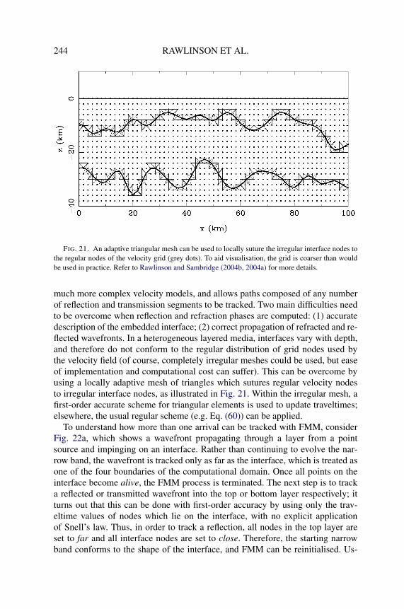
244 RAWLINSON ET AL.
FIG. 21. An adaptive triangular mesh can be used to locally suture the irregular interface nodes tothe regular nodes of the velocity grid (grey dots). To aid visualisation, the grid is coarser than wouldbe used in practice. Refer to Rawlinson and Sambridge (2004b, 2004a) for more details.
much more complex velocity models, and allows paths composed of any numberof reflection and transmission segments to be tracked. Two main difficulties needto be overcome when reflection and refraction phases are computed: (1) accuratedescription of the embedded interface; (2) correct propagation of refracted and re-flected wavefronts. In a heterogeneous layered media, interfaces vary with depth,and therefore do not conform to the regular distribution of grid nodes used bythe velocity field (of course, completely irregular meshes could be used, but easeof implementation and computational cost can suffer). This can be overcome byusing a locally adaptive mesh of triangles which sutures regular velocity nodesto irregular interface nodes, as illustrated in Fig. 21. Within the irregular mesh, afirst-order accurate scheme for triangular elements is used to update traveltimes;elsewhere, the usual regular scheme (e.g. Eq. (60)) can be applied.
To understand how more than one arrival can be tracked with FMM, considerFig. 22a, which shows a wavefront propagating through a layer from a pointsource and impinging on an interface. Rather than continuing to evolve the nar-row band, the wavefront is tracked only as far as the interface, which is treated asone of the four boundaries of the computational domain. Once all points on theinterface become alive, the FMM process is terminated. The next step is to tracka reflected or transmitted wavefront into the top or bottom layer respectively; itturns out that this can be done with first-order accuracy by using only the trav-eltime values of nodes which lie on the interface, with no explicit applicationof Snell’s law. Thus, in order to track a reflection, all nodes in the top layer areset to far and all interface nodes are set to close. Therefore, the starting narrowband conforms to the shape of the interface, and FMM can be reinitialised. Us-

SEISMIC RAY TRACING AND WAVEFRONT TRACKING 245
FIG. 22. Principle behind the multi-stage FMM scheme. Each layer represents a separate com-putational domain in which FMM is initialised either from a source or a layer boundary. (a) Incidentwavefront generated from a point source; (b) narrow band defined by a set of interface nodes; (c) re-flected wavefront tracked; (d) refracted wavefront tracked.
ing a starting narrow band that does not conform to the shape of the first-arrivingwavefront is acceptable provided it is understood that the wavefront cannot reflectfrom or transmit through the interface more than once. A refracted wavefront canbe tracked in the same way, although in this case all nodes in the bottom layerare set to far. This basic procedure can be applied iteratively to track phases com-prising any number of reflected and transmitted phases in media of virtually anycomplexity. It should be noted, however, that the arrival found in each case is theabsolute first-arrival of the specified phase, and is therefore likely to have small

246 RAWLINSON ET AL.
amplitude, particularly if it has experienced multiple interactions with complexinterfaces and velocity gradients.
Figure 23 shows an example of a reflection multiple tracked in the presenceof a highly heterogeneous velocity model. As in Fig. 19, the velocity variationsare pathological relative to real Earth structure, but the purpose of the example isto demonstrate the robustness of the method. The two-point ray-path (Fig. 23a)favours fast regions of the model and preferentially reflects from convex regionsof the interface; this is due to the fact that the first-arrival of this class of phaseis tracked. The wavefront becomes more complex as it evolves (Fig. 23b, c)in response to strong velocity contrasts and interface geometry, but the multi-stage FMM remains stable. This stability is highly desirable in many applicationsincluding seismic tomography and non-linear earthquake relocation, which typi-cally require many data prediction steps in order to obtain a solution.
In a recent paper, de Kool et al. (2006) extend the multi-stage FMM schemeto 3-D spherical coordinates. The new implementation shares many of the ba-sic principles used in the 2-D Cartesian version of Rawlinson and Sambridge(2004a), but several improvements have been implemented. These include dis-carding the explicit irregular mesh used to suture interface nodes to neighbouringvelocity nodes; in 3-D one would need to use an irregular tetrahedral mesh,which can get complicated, particularly for interfaces with high curvature. In-stead, a procedure based on testing all combinations of nodes (up to three at atime) adjacent to the node to be updated (interface node or velocity node adjacentto the interface) is used. Each combination of nodes allows a plane wave approx-imation to be made, and the one that yields the minimum traveltime is chosen.Another procedure built into the new 3-D method allows later-arriving reflec-tions such as the global PP phase to be tracked. This is done by initiating FMMfrom both source and receiver and matching reflection points using Fermat’s prin-ciple of stationary time. The flexibility of the new scheme is demonstrated inFig. 24, which shows ray paths from teleseismic and local earthquake sources(extracted from traveltime fields computed using the multi-stage FMM) in a sub-duction zone setting. [The 3-D FMM software is freely available to downloadfrom http://rses.anu.edu.au/seismology/fmmcode.]
3.2. Shortest Path Ray Tracing
Shortest path ray tracing or SPR is another popular method for determiningfirst-arrival traveltimes at all points of a gridded velocity field (Nakanishi andYamaguchi, 1986; Moser, 1991; Fischer and Lees, 1993; Cheng and House, 1996;Zhao et al., 2004; Zhou and Greenhalgh, 2005). Rather than solve a differentialequation, a network or graph is formed by connecting neighbouring nodes withtraveltime path segments. Dijkstra-like algorithms can then be used to find theshortest path between a given point and all other points in the network. According

SEISMIC RAY TRACING AND WAVEFRONT TRACKING 247
FIG. 23. A reflection multiple computed using the multi-stage FMM scheme of Rawlinson andSambridge (2004a). (a) A two point ray path corresponding to the reflection multiple, computed afterthe completion of the multi-stage FMM; (b) snapshot of the evolving wavefront. Isochrons are con-toured at 0.4 s intervals, and the leading wavefront is shown in blue; (c) same as (b) but at a later pointin time.

248 RAWLINSON ET AL.
FIG. 24. Ray paths from local earthquake and teleseismic sources, computed using the multi-stageFMM scheme of de Kool et al. (2006), in the presence of a subduction zone. Receivers are denoted byblue spheres and local earthquake sources by red diamonds. P-wave paths are blue, and S-wave pathsare green. S to P conversions occur at the upper interface of the dipping slab for the local earthquakesources.
to Fermat’s principle of stationary time, the shortest time path between two pointscorresponds to a true ray path.
Shortest path networks are commonly defined in terms of either a cell or a gridcentered framework. In a seminal paper by Nakanishi and Yamaguchi (1986), thevelocity field is defined by a set of constant velocity cells with network nodesplaced on the interface between each cell (see Fig. 25a). The advantage of thisapproach is that traveltimes between each node pair can be easily evaluated ast = ds where d is the distance between the two nodes and s is the slowness of thecell containing the ray segment. Accuracy may be increased by either reducingcell size or increasing the number of nodes on cell edges. Figure 25b illustrates aselection of minimum time ray paths from one of the nodes to several other nodesin a constant velocity medium. This example provides some intuitive understand-ing of the sources of error inherent to this approach, as the true paths would bestraight lines. Paths such as OC and OD are relatively straight, but OB and in par-ticular OA are poor approximations due to the absence of connections betweennodes on the same cell surface.
Another way of creating a network is to use a regular grid of velocity nodesand form linear connections between adjacent velocity nodes (Moser, 1991), asshown in Fig. 26a. The traveltime between two connected nodes A and B can besimply approximated by t = d(sA + sB)/2 where sA and sB are the slowness

SEISMIC RAY TRACING AND WAVEFRONT TRACKING 249
FIG. 25. Shortest path network built on a grid of constant velocity cells (Nakanishi and Yam-aguchi, 1986; Moser, 1991). In this example, two network nodes are placed on the edge of each cellboundary. (a) All allowable path connections between nodes. Thick dashed grey lines highlight theconnections from a single node; (b) shortest paths between node O and a selection of surroundingnodes in a homogeneous medium.
FIG. 26. Shortest path network built on a grid of velocity nodes (Moser, 1991). (a) A grid of25 nodes with at most 8 connections per node; (b) increasing the number of connections allows smallerpath deviations to be more accurately represented.
at nodes A and B respectively. The angular distance between branches emanatingfrom a single node in Fig. 26b is 45◦, which is relatively large. This can be reducedby increasing the number of node connections, as demonstrated in Fig. 26b. Theconnection stencil for a particular node is sometimes referred to as the “forwardstar” (Klimeš and Kvasnicka, 1994). In the case of Fig. 26a, the forward star has 8connections, while in Fig. 26b the forward star has 16 connections. The advantage

250 RAWLINSON ET AL.
FIG. 27. Three iterations of a simple shortest path scheme using a forward star with 8 connections.Grey dots have known traveltimes, black dots have trial traveltimes, and white dots are yet to havetraveltime computed.
of a grid formalism for the shortest path network is that continuously varyingvelocity fields can be more accurately represented, and interfaces are more easilyinserted.
Once a network structure and method of traveltime determination between nodepairs has been chosen, the next step is to use a shortest path algorithm to computethe full traveltime field and associated ray paths. The original network theory al-gorithm was developed by Dijkstra (1959), for which computation time scales asO(M2), where M is the number of nodes. The basic approach is conceptuallysimple, with nodes divided into two groups: a set of P nodes with known trav-eltimes, and a set of Q nodes with unknown traveltimes (Moser, 1991); initially,Q contains M elements and P is empty, with the traveltimes of nodes in Q set toan arbitrarily large value. The scheme is initiated from a source node by adding itto P , and then calculating traveltimes to all neighbouring nodes as defined by theforward star (see Fig. 27). These constitute trial traveltime values, and the methodproceeds by choosing the trial node with minimum traveltime, adding it to P andthen computing trial times to all neighbouring nodes in Q. If the node in Q alreadyhas a trial value from a previous iteration, then the one with minimum traveltimeis selected. The complete traveltime field is found in exactly M iterations, and raypaths are obtained by simply recording the update order of nodes.
The most time consuming part of the Dijkstra algorithm is locating the mini-mum traveltime node, because in its traditional usage (Moser, 1991), the entire setof nodes in Q is tested, even those with arbitrarily large values. Thus, the total op-eration count is
∑Mi=1 i = 1
2M(M + 1) → O(M2). However, it is possible to usemuch more efficient schemes such as the heap sort, which has an operation countof O(M log M), due to the ordered storage of trial traveltimes in a binary tree.Much work has been done to increase the computational speed of shortest pathalgorithms by introducing increasingly efficient sorting algorithms (Moser, 1991;Klimeš and Kvasnicka, 1994; Cheng and House, 1996; Zhang and Toksöz, 1998).
It is worth noting the similarity between SPR and eikonal solvers such as FMM,which use the shape of the first-arrival wavefront as the computational front (cf.

SEISMIC RAY TRACING AND WAVEFRONT TRACKING 251
Figs. 27 and 18). The only real difference is in the way traveltimes are updated toneighbouring nodes. Errors in SPR are due to finite node spacing and the angulardistribution of node connectors. A coarse grid of nodes may poorly approximatethe true velocity variations, while a limited range of angles between adjacent con-nectors may not allow for an accurate representation of the path. The accuracyof eikonal solvers is also a function of grid spacing, and parallels can be drawnbetween the complexity of the forward star used in SPR and the finite differencestencil used to solve the eikonal equation.
Although SPR methods can only be used to locate absolute first-arrivals incontinuous media, they can be adapted to track refracted and reflected waves inmuch the same way as eikonal methods. Moser (1991) describes a constrainedshortest path approach to computing this class of phase in layered media, whichrequires that paths visit a specified set of nodes that lie on an interface. In prin-ciple, the scheme is equivalent to the multi-stage FMM described earlier, whichseparates the medium into different computational domains. Thus, shortest pathsare computed from the source node to all other nodes in the layer; the travel-times at interface nodes are recorded and ordered in a heap; and then the layerinto which the wave propagates has all nodes placed in Q and P set to empty.The evolution of the new time field will therefore be initiated from the interfacenode with minimum traveltime. Like the multi-stage FMM, this scheme could beextended to compute paths comprising any number of reflection and refractionbranches.
SPR has proven to be effective in a number of practical seismic applicationsthat require large datasets to be predicted in the presence of significant lateralheterogeneity. In their original implementation of SPR, Nakanishi and Yamaguchi(1986) invert traveltimes from local earthquakes for 2-D velocity structure. Zhangand Toksöz (1998) use an updated version of the SPR scheme, which samplesthe wavefront with uniform angular coverage and removes unnecessary nodesfrom the network, in a 2-D refraction tomography algorithm. In 3-D, Toomey etal. (1994) invert refraction traveltimes for crustal structure using a similar SPRscheme to that proposed by Moser (1991). More recently, Bai (2005) use SPRin the inversion of local and regional earthquake traveltimes for the 3-D velocitystructure of Rabaul volcano in Papua New Guinea.
4. MULTI-ARRIVAL WAVEFRONT TRACKING
Most of the ray and grid-based schemes described previously are only suitablefor tracking a single or limited number of arrivals between two points. In manycases, the presence of velocity heterogeneity results in an evolving wavefrontself-intersecting, a phenomenon commonly referred to as multipathing, because itresults in more than one ray path passing through a given point. This behaviour is

252 RAWLINSON ET AL.
readily observed in Fig. 1. Eikonal and shortest path methods will only provide thefirst-arrival in such cases; ray tracing schemes can potentially provide more thanone arrival, but the severe non-linearity of the two-point problem makes reliabil-ity a major issue. The heterogeneity of Earth structure means that multipathingcommonly contributes to the complexity of a recorded waveform, and having ascheme that can efficiently predict all arrivals of significant amplitude has im-portant implications in various areas of seismology, such as seismic imaging. Inparticular, it has already been noted that first-arrival traveltimes, which are com-monly exploited in seismic tomography, tend to avoid regions of low wavespeed.Later arrivals, which do not necessarily exhibit such behaviour, could thereforeprovide better path coverage and consequently result in improved imaging.
To date, a number of methods have been developed to solve the multi-arrivalproblem. These include grid-based (Benamou, 1999; Steinhoff et al., 2000;Engquist et al., 2002; Fomel and Sethian, 2002; Osher et al., 2002; Symes andQian, 2003), ray-based (Vinje et al., 1993; Lambaré et al., 1996; Vinje et al.,1996, 1999) and hybrid schemes (Benamou, 1996). Due to the relative infancy ofthis branch of seismology, many of the methods that have been proposed so farare not sufficiently developed for practical application. Here, several ray and gridbased schemes are discussed.
4.1. Ray Based Schemes
One of the first ray-based schemes for computing multi-paths was proposedby Vinje et al. (1993), and is commonly referred to as wavefront construction.The basic principle underlying the method is that a wavefront can be evolved byrepeated application of local ray tracing from a set of points lying on the wavefrontsurface. Thus, for some given time step δt , a new wavefront is defined by the endpoints of the rays traced from the old wavefront, as illustrated schematically inFig. 28. In order to avoid undersampling of the wavefront as it evolves, new pointsare interpolated based on a distance criterion between adjacent rays. Thus, in orderto apply this scheme, all that is required is some initial value formulation of theray equation (e.g. Eq. (29)), an interpolation criterion and an interpolation method.From a practical implementation point of view, an efficient indexing scheme forstoring the path end points and their connectivity is also required.
The basic 2-D scheme of Vinje et al. (1993) was subsequently extended to 3-D(Vinje et al., 1996), and modified for media involving complex interface struc-tures (Vinje et al., 1999). The solution of the initial value ray tracing equationscan be computed with high accuracy, so the main source of error in the wavefrontconstruction method comes from interpolation. To decide whether a point needsto be interpolated, Vinje et al. (1993) uses a distance criterion between adjacentnodes i.e. |ri+1 − ri | � dn, where ri+1 and ri are two adjacent points on the samewavefront and dn is the distance tolerance above which a new point is interpo-lated. The problem with this interpolation criterion is that it does not account for

SEISMIC RAY TRACING AND WAVEFRONT TRACKING 253
FIG. 28. Schematic diagram illustrating the principle behind the wavefront construction schemeproposed by Vinje et al. (1993). At each iteration, a new wavefront is constructed from the previouswavefront using local ray tracing and interpolation.
variations in wavefront curvature, so regions of high detail are likely to be under-sampled. This can be ameliorated to some extent by using a criterion based onangular distance as well, but difficulties can still arise due to the presence of sharpcorners, which usually occur when a wavefront triplicates. Since most interpola-tion schemes are best applied to smooth, differentiable functions, they may notproduce satisfactory results.
An alternative approach to interpolation in physical (or “normal”) space is toinstead perform it in phase space (Lambaré et al., 1996; Hauser et al., 2006).As noted earlier, phase space is defined as (r,∇T ), where r is a point on thewavefront and ∇T is the traveltime gradient, equivalent to the ray trajectory. Ifnormal space is extended to higher dimensional phase space by using ∇T as theother coordinate directions, then the wavefront is “unfolded” into a smooth curvesometimes referred to as a “bicharacteristic strip” or curve (Osher et al., 2002).Fig. 29 shows a circular wavefront in 2-D real space unfolded into a spiral curvein 3-D reduced phase space.
Reduced phase space makes use of the relationship ∇T = f (θ, φ), where θ andφ are ray inclination and azimuth respectively (see Eq. (29)); thus, it is possibleto transform 6-D phase space into 5-D reduced phase space for problems in threedimensional normal space, and 4-D phase space into 3-D reduced phase space for

254 RAWLINSON ET AL.
FIG. 29. Representation of a circular wavefront in 3-D reduced phase space; the ray path inclina-tion θ is used as the third coordinate.
problems in two dimensional normal space. The advantage of a reduced phasespace representation is that when the wavefront self intersects and contains sharpcorners, its corresponding bicharacteristic curve in phase space will be locallysmooth and single valued, as demonstrated in Fig. 30.
In order to compute the distance between neighbouring points in reduced phasespace, it is necessary to scale the normal space coordinates so that they lie in theinterval [−π, π]; for example, in 2-D Cartesian coordinates, −π � x, y � π .This scaling correlates the metric distance with the angular distance. The criterionfor adding a new point is then given by |xi+1 − xi | � dp, where xi+1 and xi areadjacent points on the wavefront and dp is the tolerance. The important differencecompared to the criterion used by Vinje et al. (1993) is that here x = (r, θ), ratherthan x = r. The smoothness of the bicharacteristic curve in reduced phase spacemeans that linear interpolation of x (five variables in 3-D, three variables in 2-D)is often sufficient. However, it is relatively straightforward to use higher-orderinterpolators. For example, in 3-D phase space, one could insert a new point xm
midway between xi+1 and xi using a weighted average defined by (Dyn et al.,1990)
(64)xm = −xi−1 + 9xi + 9xi+1 − xi+2
16,
which provides a smoother interpolation. As well as using interpolation to in-troduce new points to the wavefront, it also makes sense to have a minimumdistance criterion to allow the removal of points which become too close togetheras a result of wavefront focusing. Properly applied, this can significantly improvecomputational efficiency without degrading accuracy.
The robustness of wavefront construction i n reduced phase space is demon-strated in Fig. 31, which shows several snapshots of an evolving wavefront

SEISMIC RAY TRACING AND WAVEFRONT TRACKING 255
FIG. 30. A triplicating wavefront in normal space is represented by a smooth bicharacteristiccurve in reduced phase space. Note that the intersecting segments in normal space no longer intersectin phase space, and the sharp corner is unfolded into a smooth segment of the bicharacteristic curve.
FIG. 31. Wavefronts tracked through the smoothed Marmousi model using the wavefront con-struction method of Hauser et al. (2006).

256 RAWLINSON ET AL.
in the smooth version of the Marmousi model. The Marmousi model is oneof the most challenging benchmarks for ray tracing and grid-based traveltimeschemes, and is frequently used to test new methods (e.g. Lambaré et al., 1996;Alkhalifah and Fomel, 2001). In the case of Fig. 31, which uses the scheme ofHauser et al. (2006), the wavefront gradually develops multiple self-intersectionsas it propagates, which is testament to the complexity of the underlying model.However, the smoothness of the corresponding bicharacteristic curve in reducedphase space ensures that the scheme remains well behaved. In this example, over60 arrivals from a single source are detected in some regions of the model.
A second wavefront construction example, which tracks a surface wavefrontfrom an earthquake in northern Papua New Guinea through the southwest Pacificregion, is shown in Fig. 32. The phase velocity model (Fig. 32a) was constructedon the basis of five dispersion curves for fundamental mode Rayleigh waves witha 15 s period, with interpolation using average local topography to create thecomplete 2-D velocity field. At very low frequencies, great circle path propagationis a reasonable approximation, but at higher frequencies, the effects of velocityvariations on path geometry should be considered. Fig. 32b shows the result ofshooting a large fan of equally spaced rays (in azimuth) from the source. Thestrong velocity gradients present in the model leads to significant multipathing,and ray coverage is highly non-uniform. Using this approach, it is not possibleto extract the shape of the evolving wavefront with much fidelity. In contrast,the phase space wavefront construction method of Hauser et al. (2006) appears tocapture the full detail of the wavefront (Fig. 32c), with many levels of triplicationsevident. All ray paths (41 in total) from the source to a station located in the SouthIsland of New Zealand are shown in Fig. 32d. Clearly, the energy received by thestation will have sampled a broad region of the velocity model, which at the veryleast suggests that a great circle path approximation for higher frequency surfacewaves would not be valid in this case.
Extension of the phase space wavefront reconstruction scheme to 3-D is nottrivial, as the connectivity between neighbouring points on a wavefront surfaceis not unique (unlike the 2-D case). Points could be connected using a triangu-lar mesh, but a carefully considered interpolation strategy would be required toproperly target regions of the wavefront that become undersampled. In addition,the use of higher order interpolation would be desirable to minimise the numberof points that are required to accurately represent the evolving wavefront. Onepossibility is to use an edge splitting strategy that subdivides adjacent trianglesthat have a common edge which exceeds some distance tolerance. The butterflysubdivision scheme of Dyn et al. (1990) works along these lines, and allows forlinear as well as higher order interpolation.
Several wavefront construction schemes have already been devised for 3-D me-dia, most notably those of Vinje et al. (1996, 1999) and Lucio et al. (1996). Bothuse triangular meshes to define the wavefront surface, although they use differ-ent interpolation strategies. In the case of Vinje et al. (1999), wavefronts can also

SEISMIC RAY TRACING AND WAVEFRONT TRACKING 257
(a) (b)
(c) (d)
FIG. 32. Surface wavefront propagation in the southwest Pacific. (a) Phase velocity model forfundamental mode Rayleigh waves with a period of 15 s; (b) rays and wavefronts computed using afan shooting scheme. Wavefronts are visualised by placing red dots along ray paths at predeterminedintervals in time. Note that there are more red dots (10,000 per time step) than rays (500) because notall rays are plotted; (c) wavefronts plotted at the same time increments as (b), but computed using thewavefront construction scheme of Hauser et al. (2006); (d) ray paths between the source and a receiverlocated in New Zealand, obtained from the wavefront construction solution.
be tracked in so called “open models” which may contain interfaces with holes.This allows multiple reflection and refraction arrivals to be computed. The useof local ray tracing to evolve the propagating wavefront means that other ray-related variables such as amplitude may also be computed (Vinje et al., 1993;Lambaré et al., 1996). Amplitude is a potentially important quantity when multi-

258 RAWLINSON ET AL.
ple paths are considered, because it offers a means of discriminating between therelative importance of each arrival.
Of all the multi-arrival schemes proposed so far, wavefront construction isby far the most developed, and is perhaps the only one that is sufficientlyrobust and efficient for practical problems. It has become a standard tool inthe exploration industry via the NORSAR-3D modelling package, which isbased on the scheme of Vinje et al. (1999), and has been used in various ap-plications including coincident reflection migration (Xu and Lambaré, 2004;Xu et al., 2004).
Another scheme for tracking multiple arrivals is “big ray-tracing” (Benamou,1996; Abgrall, 1999), which is actually a hybrid method that attempts to combineinitial value ray tracing and finite difference solution of the eikonal equation inorder to compute the multi-valued traveltime field. The first step of the procedureis to use initial value ray tracing to partition the traveltime field into single-valuedregions via a fan shoot. The second step involves computing traveltimes on anirregular grid of points that span each adjacent pair of ray paths using an eikonalsolver. This results in the complete traveltime field spanned by the ray paths beingfound, and allows wavefronts and intermediate ray paths to be extracted from thesolution. However, the principal drawback of this scheme is that the fan shoot,even with a large number of initial rays, is unlikely to properly sample the evolv-ing wavefront (as demonstrated previously in Fig. 32b); for example, the detailcontained in an evolving triplication is unlikely to be retained. Rietdijk (1999)discusses the limitations of big ray-tracing in more detail.
4.2. Grid Based Schemes
Compared to a ray-based technique such as wavefront construction, grid basedschemes are potentially attractive as they avoid the need for complex data struc-tures to track irregular ray geometries, and the use of interpolation to retain auniform sampling of the propagating wavefront. Over the last decade, a numberof new grid-based methods for tracking multi-valued wavefronts have been pro-posed, and new developments appear regularly in the current literature.
One possibility for tracking multiple arrivals is to exploit the stability and effi-ciency of first-arrival eikonal solvers by partitioning the multi-valued solution intoa series of single valued solutions in a way that is analogous to big ray-tracing.A detailed examination of this approach is given by Benamou (1999); other pa-pers on domain decomposition methods include those by Symes and Qian (2003)and Bevc (1997). The main challenge faced by these schemes is devising a ro-bust splitting strategy, as the structure of the multi-valued solution is not knowna priori. Given that many levels of triplication can occur (e.g. Figs. 31 and 32),it is difficult to envisage this approach becoming generally applicable. Benamou(2003) provides an overview of a number of different splitting methods.

SEISMIC RAY TRACING AND WAVEFRONT TRACKING 259
FIG. 33. Level set representation of an interface. In this example, the zero level set of the signeddistance function is a circle.
Recently, a number of schemes have been proposed for tracking multi-valuedwavefronts using the level set method. Level set methodology was pioneeredby Osher and Sethian (1988) for the tracking of interfaces, and has been ap-plied to various problems in the physical sciences (Sethian, 1999; Osher andFedkiw, 2003), perhaps most notably in fluid dynamics for the evolution of in-terfaces between fluids and gasses (e.g. Mulder et al., 1992; Sussman et al., 1994;Chang et al., 1996). The basic idea behind a level set formulation is to represent aninterface as the zero level set, or zero contour, of a function defined as the signeddistance from each grid point to the closest point on the interface (see Fig. 33).This implicitly represented interface can then be evolved by finite difference solu-tion of a set of partial differential equations that explicitly describe the behaviourof the signed distance function over time. In general, the level set method de-scribes the evolution of an m − 1 dimensional manifold in m dimensional space;thus, a curve is tracked on a 2-D grid of points, and a surface is tracked on a 3-Dgrid of points. Note that while the FMM scheme presented earlier is also an inter-face tracking algorithm, it deals strictly with monotonically advancing interfaces,which allows for a boundary value formulation of the problem. Level set methodsdo not have this restriction, and consequently require an initial value formulation.
If we denote the signed distance function by φ(x), then at some given pointx = xA, φ(xA) is the distance from xA to the closest point on the interface, andis negative if xA is inside the interface, and positive if xA is outside the interface(Fig. 33). The propagation of the surface implicitly described by φ(x) can bedefined in space and time by φ(r(t), t) = 0, where r(t) is the location of the zerolevel set in space at time t . The time derivative of this expression is given by thechain rule as
(65)φt + ∇φ(r(t), t
) · rt (t) = 0,

260 RAWLINSON ET AL.
where φt and rt are time derivatives of φ and r respectively. If F is defined asthe scalar speed function in the outward normal direction to the evolving surface,then F = rt (t) · n, where the unit normal direction n = ∇φ/|∇φ|. The evolutionequation for the signed distance function φ is therefore given by
(66)φt + F |∇φ| = 0,
with some given initial condition φ(x, t = 0). This is the level set equation thatwas originally formulated by Osher and Sethian (1988). The signed distance func-tion φ is well behaved when |∇φ| = 1 at every grid point in the computationaldomain. When this occurs, φt = −F , so when F > 0 the interface moves in theoutward normal direction, and when F < 0 the interface moves in the inwardnormal direction.
The signed distance function can become spatially discontinuous in gradientwhen points exist which are equidistant to at least two points on the front. Thus,numerical methods used for solving Eq. (66) must exhibit reasonable behaviour inthe presence of gradient discontinuities; fortunately, a large number of schemes,such as ENO and WENO, have been developed for solving differential equationsof this type (e.g. Osher and Shu, 1991; Jiang and Peng, 2000).
When the scalar speed function F is dependent on some vector velocity fieldv(x) defined at the grid points, then F = v · n, so Eq. (66) becomes
(67)φt + v(x) · ∇φ = 0.
The strength of the level set method lies in its implicit representation of an in-terface; topological changes like breaking and merging are handled naturally, andthere is no need for resampling of the wavefront as it evolves. However, the in-terface cannot self-intersect, which at first appears to rule out using the methodfor multi-valued wavefronts. An approach devised by Osher et al. (2002), whichovercomes this limitation, is to consider the problem in a reduced phase space,where the bicharacteristic curve is defined as the intersection of two zero level setsurfaces (see Fig. 34); these surfaces are perpendicular along their line of inter-section. The two surfaces can be separately evolved by solving the following pairof level set equations
(68)φt + v · ∇φ = 0ψt + v · ∇ψ = 0
},
where the velocity vector v is given by Eq. (29), and φ and ψ represent the twolevel set functions. The bicharacteristic curve is thus implicitly defined by thecurve φ = ψ = 0.
An example of a triplicating wavefront that is tracked using the level set ap-proach described above is shown in Fig. 35. The two zero level set surfaces ofφ and ψ are perpendicular where they intersect, and the line of intersection de-scribes the bicharacteristic curve, which can be projected into normal space toobtain the wavefront. In this case, the level set equations defined by Eq. (68)

SEISMIC RAY TRACING AND WAVEFRONT TRACKING 261
FIG. 34. In 3-D reduced phase space, the bicharacteristic curve can be described by the inter-section of two zero level set surfaces. The projection of the bicharacteristic curve into normal spaceproduces a circular wavefront in this example.
are solved using a fifth order WENO scheme in space and a third order TVDRunge–Kutta scheme in time (Hauser et al., 2006). Each signed distance functionis updated at each time step for the entire computational domain. When computedon a 51 × 31 × 51 grid using 70 time steps and a time increment of 0.1 s, the CPUtime is approximately 45 s on a 3.0 GHz Intel Pentium 4 PC running GNU/Linux;however, reducing the grid spacing by a factor of two (101 × 61 × 101 points)results in CPU time increasing to approximately 717 s. This increase can be ex-plained by two factors: first, halving the grid spacing in 3-D phase space willincrease the number of points by a factor of 8; second, the CFL criterion used(Hauser et al., 2006) requires that a surface does not cross more than one grid cellper time step. Thus, halving the grid spacing means that it is now necessary touse 140 time steps with a time increment of 0.05 s. Combined, these two factorsresult in a 16-fold increase in CPU time when grid spacing is halved.
The relationship between grid spacing and CPU time is the main limitationof the level set scheme of Osher et al. (2002). By comparison, wavefront con-struction schemes can increase the resolution of a wavefront by a factor of two(doubling the number of rays) with only a factor of two increase in CPU time(Hauser et al., 2006). For strongly curved wavefronts (e.g. Fig. 35), it is oftennecessary to have high resolution grids, as the zero level set surfaces tend to be-come more tightly folded as the wavefront evolves; if a surface overturns withinseveral grid cells or less, then information will be lost and the wavefront will bemore poorly represented. Although this scheme can be extended to 3-D by track-

262 RAWLINSON ET AL.
FIG. 35. The evolution of a triplicating wavefront computed using a level set scheme. The zerolevel set of φ is denoted by the magenta surface, and the cyan surface denotes the zero level set of ψ .The bicharacteristic curve is defined by the intersection of these two surfaces, and the projection ofthe line of intersection into (x, y) space yields the triplicating wavefront. The initial plane wavefrontenters the box at x = 0.
ing the evolution of three surfaces in five dimensions (Osher et al., 2002), thecomputational burden would be immense, because increasing grid resolution by afactor of two would increase CPU time by a factor of 64.
Despite the apparent limitations of the level set approach described above,research in this area is ongoing, with particular attention given to improv-ing the efficiency of the scheme. This can be done by using a local level setscheme which only updates the signed distance functions within a narrow bandabout the bicharacteristic curve (Osher et al., 2002; Osher and Fedkiw, 2003;Qian and Leung, 2006), and adaptive gridding, which provides higher resolutiononly where it is required. Qian and Leung (2006) devise a local level set schemewhich uses a paraxial formulation of the ray equations in which the z coordinatebecomes the independent variable. For two dimensional problems, phase spacecan therefore be defined by (x, θ) rather than (x, z, θ), which simplifies the prob-lem, but imposes limitations on path geometry (in this case, wavefronts can onlymove in the positive z direction). Using a waveguide model similar to Fig. 35 and

SEISMIC RAY TRACING AND WAVEFRONT TRACKING 263
a 120 × 120 grid, Qian and Leung (2006) show that CPU time (on a Pentium IVdesktop) is 72 minutes for a global level set method, but only 8 minutes for theirlocal level set scheme, which is a significant improvement. Other papers on levelset based methods for wavefront tracking in phase space include those by Leunget al. (2004), Qian and Leung (2004) and Cockburn et al. (2005).
An alternative approach to computing multi-arrivals with a grid-based schemehas been proposed by Fomel and Sethian (2002). Starting with the Liouvilleformulation of the ray tracing equations, a system of time-independent PDEs (re-ferred to as “Escape Equations”) are formulated which can be solved numericallyon a grid in reduced phase space. The solutions correspond to the arrival times atthe boundary from every point in the phase space domain. As a result, the com-putational efficiency of the scheme is O(M log M), where M is the total numberof grid points. Multi-arrival information such as wavefront geometry and two-point traveltimes is extracted with post-processing. In comparison with the levelset method described previously, Osher et al. (2002) claims that the Fomel andSethian (2002) scheme is less computationally efficient at each update step (by afactor of O(M1/2) in 2-D and O(M) in 3-D), but given that the Escape Equationsare boundary value PDEs, and therefore do not require solution at multiple timeincrements, it is debatable which scheme is ultimately more efficient.
It is interesting to note that a number of new schemes for computing multi-arrivals using a grid based (or “Eulerian”) framework in phase space appearedin the literature at the same time. Two of these have been discussed above, butanother, referred to as the “segment projection” method (Engquist et al., 2002),which explicitly tracks a wavefront in phase space, will also be mentioned. Inthree dimensional reduced phase space, the bicharacteristic curve is representedby its projection onto the two-dimensional xy, xθ and yθ planes. Each of thesecurves is subdivided into a contiguous set of single valued line segments. Thesegments are then evolved by solving the relevant equations of motion, with dy-namic creation and elimination of segments used to retain the minimum numberof single-valued segments necessary to represent the wavefront. The method baressome resemblance to wavefront construction in phase space, but uses an Eulerianframework. It appears to be robust in the presence of strong velocity contrasts(such as a waveguide) which cause multiple foldings of a wavefront, and Engquistet al. (2002) claim that it has a similar level of computational complexity as raytracing.
A final grid-based technique that is worth considering is Dynamic Surface Ex-tension or DSE (Steinhoff et al., 2000). DSE shares some similarities with thelevel set scheme of Osher et al. (2002), except that the grid lies in normal spaceand the information carried by each grid point is the coordinate of the closestpoint on the wavefront rather than the distance. The DSE algorithm proceeds intwo steps; in the first, the location of the wavefront is updated throughout the gridusing a knowledge of the wavefront velocity; the second step updates the wave-front location information carried by the grid. Self-intersecting wavefronts can be

264 RAWLINSON ET AL.
tracked, but not all types of wavefront behaviour can be captured (Engquist et al.,2002). In addition, the method is not purely Eulerian as interpolation is needed tomaintain an even sampling of the wavefront on the grid.
Although a number of grid and ray based schemes for tracking multi-arrivalwavefronts has been described above, our coverage has not been exhaustive. Formore information, the interested reader is directed to two relatively recent reviewpapers on the subject (Benamou, 2003; Engquist and Runborg, 2003).
5. CONCLUDING REMARKS
In this review paper, we have described a variety of schemes for tracking thekinematic evolution of high frequency seismic waves in heterogeneous 2-D and3-D structures. Where possible, we have focused on methods that have been usedin practical applications; most of these can be characterised as either ray basedor grid based. Ray tracing has traditionally been the method of choice in manyseismic applications due to its high accuracy and potential for computationalefficiency. Common ray tracing schemes include shooting, bending and pseudobending. Shooting methods formulate the kinematic ray equation as an initialvalue problem, which allows a complete ray path to be computed given an ini-tial projection vector. The boundary value problem of locating source-receivertrajectories is typically solved using iterative non-linear strategies which exploitinformation from nearby paths to update the projection parameters and better tar-get the receiver. Bending methods perturb the geometry of an initial path joiningsource and receiver, until it becomes a true (stationary) path, by iteratively solv-ing a boundary value formulation of the ray equations. Pseudo-bending schemesusually represent a path as a series of points which are perturbed using a simplealgorithm based directly on Fermat’s principle of stationary time. All three meth-ods are non-robust in the sense that the assumption of local linearity is made eventhough it is not generally valid.
Grid based methods include those that solve the eikonal equation using finitedifferences on a grid of points, and shortest path ray tracing, which uses Dijkstra-like algorithms to find traveltimes and paths through a network of nodes withpredetermined connectivity. Both techniques are capable of computing travel-times to all points of a medium in a stable and computationally efficient manner.It was shown that eikonal solvers which use the expanding wavefront as the com-putational front, such as the fast marching method, share many similarities withSPR. Compared to ray tracing, advantages of these grid based schemes includethe ability to compute traveltimes to all points of the medium in one pass, sta-bility, and in many cases, computational efficiency. However, the fact that theyonly compute the first arrival traveltime field in continuous media is a limitation,and excessive computing time can become an issue if highly accurate traveltimes

SEISMIC RAY TRACING AND WAVEFRONT TRACKING 265
are required. In addition, quantities other than traveltime are difficult to computewithout first extracting ray paths from the traveltime field and then resorting toray based techniques.
In Section 4, a variety of ray and grid based schemes for tracking multi-arrivalwavefronts were presented. Although this area of research is arguably still in itsinfancy (particularly with regard to grid-based methods), there has been a pro-liferation of new schemes appearing in the literature over the past decade. Themost developed and practical scheme to emerge so far has been wavefront con-struction, which uses local ray tracing and interpolation to advance a wavefrontsurface in discrete time steps. Of the grid-based solvers, segment projection per-haps shows the most promise, although research is still ongoing. The attractionof these techniques is that they are capable of computing all arrivals, which mayallow more of an observed seismic wavetrain to be predicted. However, from anapplication point of view, there are still significant hurdles to be overcome. Forinstance, it is almost impossible to pick arrivals other than the first from a seis-mogram unless they represent specific reflection or refraction phases. Thus, theissue of how to best exploit the multi-arrival capability of these schemes is yet tobe fully explored.
In practice, the most appropriate scheme for predicting an observational datasetdepends on a number of factors including computational efficiency, accuracy, ro-bustness and the type of information that is required. For very large datasets,computational efficiency and robustness are crucial. In cases where there are manysources and few receivers or vice-versa, then eikonal or SPR solvers should beconsidered. When lateral heterogeneity is not particularly significant and true two-point paths do not deviate significantly from those computed through a laterallyaveraged model, then shooting or bending methods of ray tracing may be moreappropriate. Global phases that penetrate deep into the Earth tend to fall into thiscategory, which perhaps explains why ray based schemes are still the preferred op-tion with this class of dataset. Traditionally, ray tracing has always been preferredin models that include interfaces, but recent developments in grid-based eikonalsolvers suggest that they can be just as effective for computing phases that experi-ence multiple refractions and reflections. In cases where multi-arrival informationis required, then a method like wavefront construction would be recommended.
In a paper by Leidenfrost et al. (1999), six different methods for calculatingtraveltimes are compared. These include three different varieties of eikonal solver,SPR, wavefront construction and a combined eikonal and Runge–Kutta method.The first of the eikonal solvers is essentially the Vidale (1988) method; the sec-ond adapts the same scheme to polar coordinates with an expanding circle ratherthan square; and the third uses the method of Podvin and Lecomte (1991). Thecombined eikonal and Runge–Kutta method solves the eikonal equation in po-lar coordinates by employing first-order finite differences in θ and a fourth-orderRunge–Kutta scheme in radius. The SPR method is that of Klimeš and Kvas-nicka (1994) and the wavefront construction scheme is essentially that of Ettrich

266 RAWLINSON ET AL.
FIG. 36. Comparison of wavefronts computed using FMM (solid lines) and WENO-DNO-PS(dashed lines) for the complex velocity model of Fig. 16. The WENO-DNO-PS scheme clearly over-estimates traveltimes in the neighbourhood of (x, z) = (80, −5) km.
and Gajewski (1996). All solvers were benchmarked in 2-D using both a simplemodel with analytic solutions and the Marmousi model. The tests show that theexpanding square eikonal solver offers the best compromise between speed andaccuracy for models that are not too complicated, while wavefront constructionproved to be the most reliable for the more complex Marmousi model. It is inter-esting to note that despite computing multi-arrivals, wavefront construction wasof the same order of accuracy as the expanding square method and had computa-tion times better than the SPR scheme.
In a separate study, Kim (2002) carry out a comparison between FMM, GMMand a second-order ENO-DNO-PS scheme using a 2-D smooth velocity model.GMM or the “Group Marching Method” (Kim, 2001), is a variant of FMMwhich avoids the need to sort narrow band traveltimes; hence computational costscales as O(M) rather than O(M log M), where M is the total number of gridpoints. As described previously, ENO-DNO-PS is an eikonal solver which usesan essentially non-oscillatory finite difference stencil, an expanding square frame-work, and post sweeping to repair causality breaches introduced by the expandingsquare. Results using the same grid spacing suggest that ENO-DNO-PS is approx-imately an order of magnitude more computationally efficient than the other twoschemes, yet produces more accurate results. However, it should be pointed outthat only first-order FMM and GMM schemes were used, and no source-grid re-finement was implemented. Another factor in favour of ENO-DNO-PS was theuse of a relatively simple velocity field; in the presence of complex velocity struc-tures, the use of ad hoc post-sweeping may not always succeed. Fig. 36 showsa comparison between the WENO-DNO-PS solution of Fig. 16 and a second-order FMM scheme with local grid refinement. Although the solutions are verysimilar, WENO-DNO-PS significantly overestimates the traveltimes in the region(x, z) = (80,−5). It is possible that a judicious post-sweeping strategy may al-

SEISMIC RAY TRACING AND WAVEFRONT TRACKING 267
leviate this problem, but in general, it is not clear that the correct solution canalways be guaranteed.
ACKNOWLEDGEMENTS
N. Rawlinson is supported by ARC Discovery Project DP0556282 and J. Hauser is supported by
ARC Discovery Project DP0451133. Most figures were created using the freely distributed software
packages GMT, xfig, Geomview and PGPLOT.
REFERENCES
Abgrall, R. (1999). Big ray-tracing and eikonal solver on unstructured grids: Application to the com-putation of a multivalued traveltime field in the Marmousi model. Geophysics 64, 230–239.
Afnimar, Koketsu, K. (2000). Finite difference traveltime calculation for head waves travelling alongan irregular interface. Geophys. J. Int. 143, 729–734.
Aki, K., Christoffersson, A., Husebye, E.S. (1977). Determination of the three-dimensional seismicstructure of the lithosphere. J. Geophys. Res. 82, 277–296.
Alkhalifah, T., Fomel, S. (2001). Implementing the fast marching eikonal solver: Spherical versusCartesian coordinates. Geophys. Prosp. 49, 165–178.
Bai, C.-Y. (2005). 3-d multi-step travel time tomography: Imaging the local, deep velocity structure ofRabaul volcano, Papua New Guinea. Phys. Earth Planet. Inter. 151, 259–275.
Bartels, R.H., Beatty, J.C., Barsky, B.A. (1987). An Introduction to Splines for Use in ComputerGraphics and Geometric Modelling. Morgan Kaufmann, Los Altos.
Benamou, J.D. (1996). Big ray tracing: Multivalued travel time field computation using viscositysolutions of the Eikonal equation. J. Comp. Phys. 128, 463–474.
Benamou, J.D. (1999). Direct computation of multivalued phase space solutions for Hamilton–Jacobiequations. Comm. Pure Appl. Math. 52, 1443–1475.
Benamou, J.D. (2003). An introduction to Eulerian Geometrical Optics (1992–2002). SIAM J. Sci.Comput. 19, 63–93.
Benz, H.M., Smith, R.B. (1984). Simultaneous inversion for lateral velocity variations and hypocen-ters in the Yellowstone region using earthquake and refraction data. J. Geophys. Res. 89, 1208–1220.
Bevc, D. (1997). Imaging complex structures with semirecursive Kirchhoff migration. Geophysics 62,577–588.
Bulant, P. (1996). Two-point ray tracing in 3-D. Pure Appl. Geophys. 148, 421–447.Bulant, P. (1999). Two-point ray-tracing and controlled initial-value ray-tracing in 3-d heterogeneous
block structures. J. Seismic Explor. 8, 57–75.Buske, S. (1999a). 3-D prestack Kirchhoff migration of the ISO89-3D data set. Pure Appl. Geo-
phys. 156, 157–171.Buske, S. (1999b). Three-dimensional pre-stack Kirchhoff migration of deep seismic reflection data.
Geophys. J. Int. 137, 1243–1260.Buske, S., Kästner, U. (2004). Efficient and accurate computation of seismic traveltime and ampli-
tudes. Geophys. Prosp. 52, 313–322.Cao, S., Greenhalgh, S. (1994). Finite-difference solution of the eikonal equation using an efficient,
first-arrival, wavefront tracking scheme. Geophysics 59, 632–643.

268 RAWLINSON ET AL.
Cassell, B.R. (1982). A method for calculating synthetic seismograms in laterally varying media.Geophys. J. Royal Astr. Soc. 69, 339–354.
Cervený, V. (1987). Ray tracing algorithms in three-dimensional laterally varying layered structures.In: Nolet, G. (Ed.), Seismic Tomography: With Applications in Global Seismology and ExplorationGeophysics. D. Reidel, Dordrecht, pp. 99–133.
Cervený, V. (2001). Seismic Ray Theory. Cambridge University Press, Cambridge.Cervený, V., Firbas, P. (1984). Numerical modelling and inversion of travel times of seismic body
waves in inhomogeneous anisotropic media. Geophys. J. Royal Astr. Soc. 76, 41–51.Cervený, V., Pšencik, I. (1983). Gaussian beams and paraxial ray approximation in three-dimensional
elastic inhomogeneous media. J. Geophys. 53, 1–15.Cervený, V., Klimeš, L., Pšencik, I. (1984). Paraxial ray approximations in the computation of seismic
wavefields in inhomogeneous media. Geophys. J. Royal Astr. Soc. 79, 89–104.Cervený, V., Klimes, L., Psencik, I. (2006). Seismic ray method: Recent developments. Adv. Geo-
phys. 48, 1–126.Chang, Y.C., Hou, T.Y., Merriman, B., Osher, S. (1996). A level set formulation of Eulerian interface
capturing methods for incompressible fluid flows. J. Comp. Phys. 124, 449–464.Chapman, C. (2004). Fundamentals of Seismic Wave Propagation. Cambridge University Press, Cam-
bridge.Cheng, N., House, L. (1996). Minimum traveltime calculations in 3-D graph theory. Geophysics 61,
1895–1898.Chiu, S.K.L., Kanasewich, E.R., Phadke, S. (1986). Three-dimensional determination of structure and
velocity by seismic tomography. Geophysics 51, 1559–1571.Chopp, D.L. (2001). Some improvements of the fast marching method. SIAM J. Sci. Comput. 23,
230–244.Cockburn, B., Qian, J., Reitich, F., Wang, J. (2005). An accurate spectral/discontinuous finite-element
formulation of a phase-space-based level set approach to geometrical optics. J. Comp. Phys. 208,175–195.
Curtis, A., Snieder, R. (1997). Reconditioning inverse problems using the genetic algorithm and re-vised parameterization. Geophysics 62, 1524–1532.
Day, A.J., Peirce, C., Sinha, M.C. (2001). Three-dimensional crustal structure and magma chambergeometry at the intermediate-spreading, back-arc Valu Fa Ridge, Lau Basin – results of a wide-angle seismic tomographic inversion. Geophys. J. Int. 146, 31–52.
Debski, W., Ando, M. (2004). Spectral ray tracer: A class of accurate two-point ray tracers. ActaGeophysica Polonica 52, 1–14.
de Kool, M., Rawlinson, N., Sambridge, M. (2006). A practical grid based method for tracking multi-ple refraction and reflection phases in 3d heterogeneous media. Geophys. J. Int. 167, 253–270.
Dijkstra, E.W. (1959). A note on two problems in connection with graphs. Numer. Math. 1, 269–271.Dyn, N., Levin, D., Gregory, J.A. (1990). A butterfly subdivision scheme for surface interpolation
with tension control. ACM Transaction on Graphics 9, 160–169.Dziewonski, A.M., Hager, B.H., O’Connell, R.J. (1977). Large-scale heterogeneities in the lower man-
tle. J. Geophys. Res. 82, 239–255.Eberhart-Phillips, D. (1986). Three-dimensional velocity structure in northern California coast ranges
from inversion of local earthquake arrival times. Bull. Seism. Soc. Am. 76, 1025–1052.Eberhart-Phillips, D. (1990). Three-dimensional P and S velocity structure in the Coalinga Region,
California. J. Geophys. Res. 95, 15,343–15,363.Eberhart-Phillips, D., Reyners, M. (1997). Continental subduction and three-dimensional crustal struc-
ture: The northern South Island, New Zealand. J. Geophys. Res. 102, 11,848–11,861.Engquist, B., Runborg, O. (2003). Computational high frequency wave propagation. Acta Numer-
ica 12, 181–266.Engquist, B., Runborg, O., Tornberg, A.-K. (2002). High-frequency wave propagation by the segment
projection method. J. Comp. Phys. 178, 373–390.

SEISMIC RAY TRACING AND WAVEFRONT TRACKING 269
Ettrich, N., Gajewski, D. (1996). Wave front construction in smooth media for prestack depth migra-tion. Pageoph 148, 481–502.
Farra, V., Madariaga, R. (1987). Seismic waveform modelling in heterogeneous media by ray pertur-bation theory. J. Geophys. Res. 92, 2697–2712.
Farra, V., Madariaga, R. (1988). Non-linear reflection tomography. Geophys. J. 95, 135–147.Fischer, R., Lees, J.M. (1993). Shortest path ray tracing with sparse graphs. Geophysics 58, 987–996.Fomel, S., Sethian, J.A. (2002). Fast-phase space computation of multiple arrivals. Proc. Nat. Acad.
Sci. 99, 7329–7334.Graeber, F.M., Asch, G. (1999). Three-dimensional models of P wave velocity and P -to-S velocity
ratio in the southern central Andes by simultaneous inversion of local earthquake data. J. Geophys.Res. 104, 20,237–20,256.
Gray, S.H., May, W.P. (1994). Kirchhoff migration using eikonal equation traveltimes. Geophysics 59,810–817.
Hammer, P.T.C., Dorman, L.M., Hildebrand, J.A., Cornuelle, B.D. (1994). Jasper Seamount structure:Seafloor seismic refraction tomography. J. Geophys. Res. 99, 6731–6752.
Hauser, J., Sambridge, M., Rawlinson, N. (2006). Phase space methods for multi arrival wavefronts.Explor. Geophys. 37, 331–339.
Hildebrand, J.A., Dorman, L.M., Hammer, P.T.C., Schreiner, A.E., Cornuelle, B.D. (1989). Seismictomography of Jasper Seamount. Geophys. Res. Lett. 16, 1355–1358.
Hole, J.A. (1992). Nonlinear high-resolution three-dimensional travel-time tomography. J. Geophys.Res. 97, 6553–6562.
Hole, J.A., Zelt, B.C. (1995). 3-D finite-difference reflection travel times. Geophys. J. Int. 121, 427–434.
Iyer, H., Hirahara, K. (1993). Seismic Tomography: Theory and Practice. Chapman & Hall, London.Jeffreys, H., Swirles, B. (1966). Methods of Mathematical Physics. Cambridge University Press, Cam-
bridge.Jiang, G.S., Peng, D.P. (2000). Weighted ENO schemes for Hamilton–Jacobi equations. SIAM J. Sci.
Comput. 21, 2126–2143.Jiang, G.S., Shu, C. (1996). Efficient implementation of weighted ENO schemes. J. Comp. Phys. 126,
202–228.Julian, B.R., Gubbins, D. (1977). Three-dimensional seismic ray tracing. J. Geophys. 43, 95–113.Kim, S. (2001). An O(N) level set method for eikonal equations. SIAM J. Sci. Comput. 22, 2178–
2193.Kim, S. (2002). 3-D eikonal solvers: First-arrival traveltimes. Geophysics 67, 1225–1231.Kim, S., Cook, R. (1999). 3D traveltime computation using second-order ENO scheme. Geo-
physics 64, 1867–1876.Kimmel, R., Sethian, J.A. (1998). Fast marching methods on triangulated domains. Proc. Nat. Acad.
Sci. 95, 8341–8435.Kirkpatrick, S., Gelatt Jr, C.D., Vecchi, M.P. (1983). Optimization by simulated annealing. Sci-
ence 220, 671–680.Klimeš, L. (1989). Gaussian packets in the computation of seismic wavefields. Geophys. J. Int. 99,
421–433.Klimeš, L., Kvasnicka, M. (1994). 3-D network ray tracing. Geophys. J. Int. 116, 726–738.Koketsu, K., Sekine, S. (1998). Pseudo-bending method for three-dimensional seismic ray tracing in
a spherical earth with discontinuities. Geophys. J. Int. 132, 339–346.Kreyszig, E. (1993). Advanced Engineering Mathematics. John Wiley & Sons, Inc., New York.Lambaré, G., Lucio, P.S., Hanyga, A. (1996). Two-dimensional multivalued traveltime and amplitude
maps by uniform sampling of a ray field. Geophys. J. Int. 125, 584–598.Langan, R.T., Lerche, I., Cutler, R.T. (1985). Tracing of rays through heterogeneous media: An accu-
rate and efficient procedure. Geophysics 50, 1456–1465.Leidenfrost, A., Ettrich, N., Gajewski, D., Kosloff, D. (1999). Comparison of six different methods
for calculating traveltimes. Geophys. Prosp. 47, 269–297.

270 RAWLINSON ET AL.
Leung, S., Osher, S.J., Qian, J. (2004). A level set method for three-dimensional paraxial geometricaloptics with multiple point sources. Commun. Math. Sci. 2, 643–672.
Li, X.G., Ulrych, T.J. (1993). Traveltime computation in discrete heterogeneous layered media. J. Seis-mic Explor. 2, 305–318.
Liu, X., Osher, S., Chan, T. (1994). Weighted essentially non-oscillatory schemes. J. Comp. Phys. 115,200–212.
Lucio, P.S., Lambaré, G., Hanyga, A. (1996). 3D multivalued travel time and amplitude maps. Pa-geoph 148, 449–479.
McCaughey, M., Singh, S.C. (1997). Simultaneous velocity and interface tomography of normal-incidence and wide-aperture seismic traveltime data. Geophys. J. Int. 131, 87–99.
Michelini, A. (1995). An adaptive-grid formalism for traveltime tomography. Geophys. J. Int. 121,489–510.
Moser, T.J. (1991). Shortest path calculation of seismic rays. Geophysics 56, 59–67.Mulder, W., Osher, S., Sethian, J.A. (1992). Computing interface motion in compressible gas dynam-
ics. J. Comp. Phys. 100, 209–228.Nakanishi, I. (1985). Three-dimensional structure beneath the Hokkaido–Tohoku region as derived
from a tomographic inversion of P -arrival times. J. Phys. Earth 33, 241–256.Nakanishi, I., Yamaguchi, K. (1986). A numerical experiment on nonlinear image reconstruction from
first-arrival times for two-dimensional island arc structure. J. Phys. Earth 34, 195–201.Neele, F., VanDecar, J., Snieder, R. (1993). The use of P wave amplitude data in a joint inversion with
travel times for upper mantle velocity structure. J. Geophys. Res. 98, 12,033–12,054.Nolet, G. (1987). Waveform tomography. In: Nolet, G. (Ed.), Seismic Tomography: With Applications
in Global Seismology and Exploration Geophysics. D. Reidel, Dordrecht, pp. 301–322.Osher, S., Cheng, L.-T., Kang, M., Shim, H., Tsai, Y.-H. (2002). Geometric optics in a phase-space-
based level set and Eulerian framework. J. Comp. Phys. 179, 622–648.Osher, S., Fedkiw, R. (2003). Level Set Methods and Dynamic Implicit Surfaces, 2nd ed. Springer-
Verlag.Osher, S., Sethian, J. (1988). Fronts propagating with curvature dependent speed: Algorithms based
on Hamilton–Jacobi formulations. J. Comp. Phys. 79, 12–49.Osher, S., Shu, C.W. (1991). High-order essentially nonoscillatory schemes for Hamilton–Jacobi
equations. SIAM J. Numer. Anal. 28, 907–922.Pereyra, V. (1996). Modelling, ray tracing, and block nonlinear travel-time inversion in 3d. Pure Appl.
Geophys. 148, 345–386.Pereyra, V., Lee, W.H.K., Keller, H.B. (1980). Solving two-point seismic-ray tracing problems in a
heterogeneous medium. Bull. Seism. Soc. Am. 70, 79–99.Podvin, P., Lecomte, I. (1991). Finite difference computation of traveltimes in very contrasted velocity
models: a massively parallel approach and its associated tools. Geophys. J. Int. 105, 271–284.Popovici, A.M., Sethian, J.A. (2002). 3-D imaging using higher order fast marching traveltimes. Geo-
physics 67, 604–609.Prothero, W.A., Taylor, W.J., Eickemeyer, J.A. (1988). A fast, two-point, three-dimensional raytracing
algorithm using a simple step search method. Bull. Seism. Soc. Am. 78, 1190–1198.Pulliam, J., Snieder, R. (1996). Fast, efficient calculation of rays and travel times with ray perturbation
theory. J. Acoust. Soc. Am. 99, 383–391.Qian, J., Leung, S. (2004). A level set based eulerian method for paraxial multivalued traveltimes.
J. Comp. Phys. 197, 711–736.Qian, J., Leung, S. (2006). A local level set method for paraxial geometrical optics. SIAM J. Sci.
Comput. 28, 206–223.Qian, J., Symes, W.W. (2002). An adaptive finite-difference method for traveltimes and amplitudes.
Geophysics 67, 167–176.Qin, F., Luo, Y., Olsen, K.B., Cai, W., Schuster, G.T. (1992). Finite-difference solution of the eikonal
equation along expanding wavefronts. Geophysics 57, 478–487.

SEISMIC RAY TRACING AND WAVEFRONT TRACKING 271
Rawlinson, N., Houseman, G.A. (1998). Inversion for interface structure using teleseismic traveltimeresiduals. Geophys. J. Int. 133, 756–772.
Rawlinson, N., Sambridge, M. (2003a). Irregular interface parameterization in 3-D wide-angle seismictraveltime tomography. Geophys. J. Int. 155, 79–92.
Rawlinson, N., Sambridge, M. (2003b). Seismic traveltime tomography of the crust and lithosphere.Advances in Geophysics 46, 81–198.
Rawlinson, N., Sambridge, M. (2004a). Multiple reflection and transmission phases in complex lay-ered media using a multistage fast marching method. Geophysics 69, 1338–1350.
Rawlinson, N., Sambridge, M. (2004b). Wavefront evolution in strongly heterogeneous layered mediausing the Fast Marching Method. Geophys. J. Int. 156, 631–647.
Rawlinson, N., Houseman, G.A., Collins, C.D.N. (2001a). Inversion of seismic refraction and wide-angle reflection traveltimes for 3-D layered crustal structure. Geophys. J. Int. 145, 381–401.
Rawlinson, N., Houseman, G.A., Collins, C.D.N., Drummond, B.J. (2001b). New evidence of Tasma-nia’s tectonic history from a novel seismic experiment. Geophys. Res. Lett. 28, 3337–3340.
Rawlinson, N., Kennett, B.L.N., Heintz, M. (2006a). Insights into the structure of the upper mantlebeneath the Murray basin from 3-d teleseismic tomography. Australian J. Earth Sci. 53, 595–604.
Rawlinson, N., Reading, A.M., Kennett, B.L.N. (2006b). Lithospheric structure of Tasmania from anovel form of teleseismic tomography. J. Geophys. Res. 111, doi:10.1029/2005JB003803.
Riahi, M.A., Juhlin, C. (1994). 3-D interpretation of reflected arrival times by finite-difference tech-niques. Geophysics 59, 844–849.
Riahi, M.A., Lund, C.E., Pederson, L.B. (1997). Three-dimensional image of the Moho undulationsbeneath the Gulf of Bothnia using wide-angle seismic data. Geophys. J. Int. 129, 461–471.
Rietdijk, R.H. (1999). Notes on big ray tracing. J. Comp. Phys. 148, 149–168.Sadeghi, H., Suzuki, S., Takenaka, H. (1999). A two-point, three-dimensional seismic ray tracing
using genetic algorithms. Phys. Earth Planet. Inter. 113, 355–365.Saltzer, R.L., Humphreys, E.D. (1997). Upper mantle P wave velocity structure of the eastern Snake
River Plain and its relationship to geodynamic models of the region. J. Geophys. Res. 102, 11,829–11,841.
Sambridge, M.S. (1990). Non-linear arrival time inversion: Constraining velocity anomalies by seek-ing smooth models in 3-D. Geophys. J. Int. 102, 653–677.
Sambridge, M., Faletic, R. (2003). Adaptive whole Earth tomography. Geochem. Geophys. Geosyst. 4,doi:10.1029/2001GC000213.
Sambridge, M., Gudmundsson, O. (1998). Tomographic systems of equations with irregular cells.J. Geophys. Res. 103, 773–781.
Sambridge, M.S., Kennett, B.L.N. (1990). Boundary value ray tracing in a heterogeneous medium:A simple and versatile algorithm. Geophys. J. Int. 101, 157–168.
Sambridge, M., Rawlinson, N. (2005). Seismic tomography with irregular meshes. In: Levander, A.,Nolet, G. (Eds.), In: Seismic Earth: Array Analysis of Broadband Seismograms, vol. 157. Ameri-can Geophysical Union, pp. 49–65.
Sambridge, M.S., Braun, J., McQueen, H. (1995). Geophysical parameterization and interpolation ofirregular data using natural neighbours. Geophys. J. Int. 122, 837–857.
Scott, J.S., Masters, T.G., Vernon, F.L. (1994). 3-D velocity structure of the San Jacinto fault zonenear Anza, California-I. P waves. Geophys. J. Int. 119, 611–626.
Sethian, J.A. (1996). A fast marching level set method for monotonically advancing fronts. Proc. Nat.Acad. Sci. 93, 1591–1595.
Sethian, J.A. (1999). Level Set Methods and Fast Marching Methods. Cambridge University Press,Cambridge.
Sethian, J.A. (2001). Evolution, implementation, and application of level set and fast marching meth-ods for advancing fronts. J. Comp. Phys. 169, 503–555.
Sethian, J.A., Popovici, A.M. (1999). 3-D traveltime computation using the fast marching method.Geophysics 64, 516–523.

272 RAWLINSON ET AL.
Shapiro, N.M., Campillo, M., Stehly, L., Ritzwoller, M.H. (2005). High-resolution surface wave to-mography from ambient seismic noise. Science 307, 1615–1618.
Shu, C.-W., Osher, S. (1988). Efficient implementation of essentially non-oscillatory shock-capturingschemes. J. Comp. Phys. 77, 439–471.
Shu, C.-W., Osher, S. (1989). Efficient implementation of essentially non-oscillatory shock-capturingschemes, ii. J. Comp. Phys. 83, 32–78.
Slawinski, M.A., Slawinski, R.A., Brown, R.J., Parkin, J.M. (2000). A generalized form of Snell’s lawin anisotropic media. Geophysics 65, 632–637.
Smith, W.H.F., Wessel, P. (1990). Gridding with continuous curvature splines in tension. Geo-physics 55, 293–305.
Snieder, R., Sambridge, M. (1992). Ray perturbation theory for traveltimes and ray paths in 3-d het-erogeneous media. Geophys. J. Int. 109, 294–322.
Snieder, R., Spencer, C. (1993). A unified approach to ray bending, ray perturbation and paraxial raytheories. Geophys. J. Int. 115, 456–470.
Spakman, W., Bijwaard, H. (2001). Optimization of cell parameterizations for tomographic inverseproblems. Pure Appl. Geophys. 158, 1401–1423.
Steck, L.K., Thurber, C.H., Fehler, M., Lutter, W.J., Roberts, P.M., Baldridge, W.S., Stafford, D.G.,Sessions, R. (1998). Crust and upper mantle P wave velocity structure beneath Valles caldera,New Mexico: Results from the Jemez teleseismic tomography experiment. J. Geophys. Res. 103,24,301–24,320.
Steinhoff, J., Fan, M., Wang, L. (2000). A new Eulerian method for the computation of propagatingshort acoustic and electromagnetic pulses. J. Comp. Phys. 157, 683–706.
Sussman, S., Smereka, P., Osher, S.J. (1994). A level set approach for computing solutions to incom-pressible two-phase flow. J. Comp. Phys. 114, 146–159.
Symes, W.W., Qian, J. (2003). A slowness matching Eulerian method for multivalued solutions ofeikonal equations. SIAM J. Sci. Comput. 19, 501–526.
Thomson, C.J., Gubbins, D. (1982). Three-dimensional lithospheric modelling at NORSAR: linearityof the method and amplitude variations from the anomalies. Geophys. J. Royal Astr. Soc. 71, 1–36.
Thurber, C.H. (1983). Earthquake locations and three-dimensional crustal structure in the Coyote Lakearea, central California. J. Geophys. Res. 88, 8226–8236.
Thurber, C.H., Ellsworth, W.L. (1980). Rapid solution of ray tracing problems in heterogeneous me-dia. Bull. Seism. Soc. Am. 70, 1137–1148.
Toomey, D.R., Solomon, S.C., Purdy, G.M. (1994). Tomographic imaging of the shallow crustal struc-ture of the East Pacific Rise at 9◦30′N. J. Geophys. Res. 99, 24,135–24,157.
Um, J., Thurber, C. (1987). A fast algorithm for two-point seismic ray tracing. Bull. Seism. Soc.Am. 77, 972–986.
van Trier, J., Symes, W.W. (1991). Upwind finite-difference calculation of traveltimes. Geophysics 56,812–821.
VanDecar, J.C., James, D.E., Assumpção, M. (1995). Seismic evidence for a fossil mantle plumebeneath South America and implications for plate driving forces. Nature 378, 25–31.
Velis, D.R., Ulrych, T.J. (1996). Simulated annealing two-point ray tracing. Geophys. Res. Lett. 23,201–204.
Velis, D.R., Ulrych, T.J. (2001). Simulated annealing ray tracing in complex three-dimensional media.Geophys. J. Int. 145, 447–459.
Vesnaver, A., Böhm, G., Madrussani, G., Rossi, G., Granser, H. (2000). Depth imaging and velocitycalibration by 3D adaptive tomography. First Break 18, 303–312.
Vidale, J.E. (1988). Finite-difference calculations of traveltimes. Bull. Seism. Soc. Am. 78, 2062–2076.Vidale, J.E. (1990). Finite-difference calculations of traveltimes in three dimensions. Geophysics 55,
521–526.Vinje, V., Åstebøl, K., Iversen, E., Gjøystdal, H. (1999). 3-D ray modelling by wavefront construction
in open models. Geophys. Prosp. 64, 1912–1919.

SEISMIC RAY TRACING AND WAVEFRONT TRACKING 273
Vinje, V., Iversen, E., Åstebøl, K., Gjøystdal, H. (1996). Estimation of multivalued arrivals in 3Dmodels using wavefront construction – Part I. Geophys. Prosp. 44, 819–842.
Vinje, V., Iversen, E., Gjøystdal, H. (1993). Traveltime and amplitude estimation using wavefrontconstruction. Geophysics 58, 1157–1166.
Virieux, J., Farra, F. (1991). Ray tracing in 3-d complex isotropic media: An analysis of the problem.Geophysics 56, 2057–2069.
Wang, Y., Houseman, G.A. (1994). Inversion of reflection seismic amplitude data for interface geom-etry. Geophys. J. Int. 117, 92–110.
Wang, Y., Pratt, R.G. (1997). Sensitivities of seismic traveltimes and amplitudes in reflection tomog-raphy. Geophys. J. Int. 131, 618–642.
White, D.J. (1989). Two-dimensional seismic refraction tomography. Geophys. J. 97, 223–245.Wiggins, S.M., Dorman, L.M., Cornuelle, B.D., Hildebrand, J.A. (1996). Hess deep rift valley struc-
ture from seismic tomography. J. Geophys. Res. 101, 22,335–22,353.Williamson, P.R. (1990). Tomographic inversion in reflection seismology. Geophys. J. Int. 100, 255–
274.Xu, S., Lambaré, G. (2004). Fast migration/inversion with multivalued rayfields: Part 1 – Method,
validation test, and application in 2D to Marmousi. Geophysics 69, 1311–1319.Xu, S., Lambaré, G., Calandra, H. (2004). Fast migration/inversion with multivalued rayfields: Part 1
– Applications to the 3d seg/eage salt model. Geophysics 69, 1320–1328.Yao, H., van der Hilst, R.D., de Hoop, M.V. (2006). Surface-wave array tomography in SE Tibet from
ambient seismic noise and two-station analysis – I. Phase velocity maps. Geophys. J. Int. 166,732–744.
Zelt, B.C., Ellis, R.M., Zelt, C.A., Hyndman, R.D., Lowe, C., Spence, G.D., Fisher, M.A. (2001).Three-dimensional crustal velocity structure beneath the Strait of Georgia, British Columbia. Geo-phys. J. Int. 144, 695–712.
Zelt, C.A. (1996). Seismic velocity structure of the central Chilean margin near the subducting JuanFernández ridge: effective inversion of traveltime data across complex, laterally varying structure.In: Abstracts. 7th Int. Symp., Deep Seismic Profiling of the Continents. Asilomar, CA.
Zelt, C.A. (1999). Modelling strategies and model assessment for wide-angle seismic traveltime data.Geophys. J. Int. 139, 183–204.
Zelt, C.A., Barton, P.J. (1998). Three-dimensional seismic refraction tomography: A comparison oftwo methods applied to data from the Faeroe Basin. J. Geophys. Res. 103, 7187–7210.
Zelt, C.A., Smith, R.B. (1992). Seismic traveltime inversion for 2-D crustal velocity structure. Geo-phys. J. Int. 108, 16–34.
Zhang, J., Rector III, J.W., Hoversten, G. (2005). Eikonal solver in the celerity domain. Geophys. J.Int. 162, 1–8.
Zhang, J., Toksöz, M.N. (1998). Nonlinear refraction traveltime tomography. Geophysics 63, 1726–1737.
Zhao, A., Zhongjie, Z., Teng, J. (2004). Minimum travel time tree algorithm for seismic ray tracing:improvement in efficiency. J. Geophys. Eng. 1, 245–251.
Zhao, D., Hasegawa, A., Horiuchi, S. (1992). Tomographic imaging of P and S wave velocity structurebeneath Northeastern Japan. J. Geophys. Res. 97, 19,909–19,928.
Zhou, B., Greenhalgh, S.A. (2005). ‘Shortest path’ ray tracing for most general 2d/3d anisotropicmedia. J. Geophys. Eng. 2, 54–63.

This page intentionally left blank

SUBJECT INDEX
Abyssal T phase 14, 16, 18, 19, 24, 25, 29,48
Accelerating moment release (AMR) 67–69, 81, 82, 90, 92, 94, 97, 118, 122,127, 134, 149, 150, 160, 181, 190
Aftershock 13, 30, 38, 39, 48, 50, 53, 79,80, 83, 84, 115, 137, 178, 190
– sequences 71Aleutian earthquake of 29 July1965 18Analytic ray tracing 211, 215Anisotropic media 206, 208, 209, 218, 220
BBackground seismicity 83, 88, 94, 128,
140, 145, 185Bending method 227, 228, 232Benioff strain 114Bicharacteristic curve 253–256, 260–263Bicharacteristic strip 253Big ray-tracing 258Boundary conditions 20, 22Boundary value problem 214, 221, 223,
225, 232, 233Butterfly subdivision 256
Cc-value 97, 103, 170, 181Causality 235, 236, 239, 266Celerity domain 242Chebyshev polynomials 233Christoffel matrix 208Constant velocity block 211Continuum damage model 125, 128Conversion– abyssal 46– downslope 8, 9, 27– seismo-acoustic 7Convex hull 219, 220Critical point 121, 127, 137Cubic B-spline 211–213, 217, 219
DDeclustering 101, 113, 115Dijkstra algorithm 246, 250, 264Downslope– T phase 14, 18– conversion model 9Dynamic Surface Extension (DSE) 263
EEarthquake– 1896 Sanriku 39– 1944 Bolivian 11, 13– 1946 Aleutian 39– 1958 Fairweather, Alaska 37, 42– 1975 Kuriles 39– 1977 Tonga 42– 1992 Nicaragua 39– 1996 Chimbote, Peru 39, 40, 51– 1996 Loihi 12– 2004 Sumatra 3, 51, 53, 55– 2005 Sumatra 54– forecast 141, 150, 190– prediction 141, 145, 149, 183Earthquake source 2, 4, 24, 32, 37, 39Eikonal equation 205, 206, 208, 214, 234,
238, 242, 258, 264Eikonal solver 234, 237, 238, 241, 243,
251, 258, 264–266Elastic wave equation 205, 206, 208Epidemic-Type Aftershock Sequence 80– model 122, 128, 177Equatorial Pacific Hydrophone Array
(EPHA) 30Escape equations 263Essentially Non-Oscillatory (ENO) 236,
237, 260, 266ETAS model 81Euler–Lagrange equation 207, 228Expanding 237– square 234–237, 266
FFalse position, method of 222Fast Marching Method (FMM) 238–248,
251, 266Fermat’s principle 207, 227, 229, 230, 232,
243, 246, 248Fiber-bundle model 124, 128Forward star 249–251Fourier series 213Fractal 134, 177
GGenetic algorithm 232, 233Group Marching Method (GMM) 266
275

276 SUBJECT INDEX
Gutenberg–Richter– law 80, 90, 118, 130, 137, 168, 178
HHamilton equations 208, 209, 218Heap sort 241, 250High frequency approximation 205, 206Homestead Valley earthquake 83Huygen’s principle 236
IInitial value problem 214, 215Irregular parameterisation 214
KKinematic ray equation 207, 216, 218, 227
LLevel set method 259–263Liouville formulation 263Loading 77, 85, 127, 137, 168, 183, 190Local grid refinement 241, 266
MMarmousi model 255, 256, 266Mogi Doughnut 90, 92, 157Monte Carlo method 99, 161, 171, 178Multi-arrival 252, 263Multi-valued traveltime field 258Multipathing 238, 251, 252, 256
NNarrow band 240, 241, 243–245, 262, 266New Madrid seismic zone 136, 182Newton’s method 220–223
OOmori law 80, 115, 123
PParaxial ray tracing 224, 225Phase space 218, 253–256, 261–263Polynesian Seismic Network (RSP) 13Power-law 43, 97, 118, 119, 127, 133, 134,
153, 160, 181, 185, 190Precursory seismicity 68, 94, 98, 111, 129,
135, 140, 145, 153Preshock 79, 81Pseudo-bending method 229, 232Pseudo-linear interpolation 211
QQuiescence 94, 122
RRate-and-state– equation 78, 84– function 144Ray perturbation theory 233Recurrence time 67, 140, 155Reduced phase space 218, 253–256, 260,
261, 263Reflection multiple 246, 247Renormalisation Group theory 123, 128Runge–Kutta method 208, 216, 217, 261,
265
SSegment projection 263Seismic cycle 85, 127, 153Seismic source 4, 6, 14, 27, 29, 34, 38, 39,
42, 48, 51, 55Self-organised criticality 118, 119, 122,
127Shooting method 214, 221–225, 227Shortest path method 246, 248–252, 264Simplex method 232Simulated annealing 227Snell’s law 207, 213, 215, 220, 243, 244SOFAR channel 2, 9, 11, 12, 19, 20, 22, 34,
37, 44SOund Fixing And Ranging technigue (SO-
FAR) 2, 6, 14, 19, 20, 22–25, 37, 44Solid–liquid interface 3, 7, 9, 15Sound Surveillance System (SOSUS) 29,
57Spectral parameterisation 213Spectral ray tracer 233Stoneley waves 15Stress– absolute 87, 88– Coulomb 71, 88– failure 87– interactions 69, 111, 145, 155– loading 111, 112– pre-– – field, 72, 85, 103, 190– shadow 72, 78, 87, 127, 128, 131, 133,
135– transfer 51, 53, 67–69, 70, 142, 144, 190– – static 70– triggering 69, 71, 77, 78, 83, 95, 111,
112, 137, 141

SUBJECT INDEX 277
Stress Accumulation model (SAM) 67, 85,90, 98, 128, 136, 137, 153, 157, 184,190
Subduction zone 13, 46, 47Sumatra–Java subduction zone 67Surface waves 15Swallowtail 239Synthetic catalog 90, 99, 100, 178
TT -Phase Energy Flux (TPEF) 37, 38, 42Tectonic memory 88Teleseismic 30, 33, 42T phase 1, 2, 8, 11–13, 15, 16, 18, 19, 22,
27, 28, 57
– duration 36– energy flux 33, 37Transport equation 206Triplicating wavefront 255, 260, 262Tsunami– earthquake 38, 39, 42, 48, 51, 56– generation 1T wave 1, 2, 4, 7–9, 11, 13, 28, 37, 48, 56
WWavefront construction 252–258, 261Waveguide model 262Weighted Essentially Non-Oscillatory
(WENO) 236, 237, 260, 261, 266

This page intentionally left blank