advances in the particle ﬁnite element method for the ... · description and the fic formulation...

ARTICLE IN PRESS

www.elsevier.com/locate/cma

Comput. Methods Appl. Mech. Engrg. xxx (2007) xxx–xxx

Advances in the particle finite element method for the analysis offluid–multibody interaction and bed erosion in free surface flows

Eugenio Onate *, Sergio R. Idelsohn 1, Miguel A. Celigueta, Riccardo Rossi

International Center for Numerical Methods in Engineering (CIMNE), Technical University of Catalonia, Campus Norte UPC, 08034 Barcelona, Spain

Received 16 November 2006; received in revised form 1 June 2007; accepted 4 June 2007

Abstract

We present some advances in the formulation of the particle finite element method (PFEM) for solving complex fluid–structure inter-action problems with free surface waves. In particular, we present extensions of the PFEM for the analysis of the interaction between acollection of bodies in water allowing for frictional contact conditions at the fluid–solid and solid–solid interfaces via mesh generation.An algorithm to treat bed erosion in free surface flows is also presented. Examples of application of the PFEM to solve a number offluid–multibody interaction problems involving splashing of waves, large motions of floating and submerged bodies and bed erosion sit-uations are given.� 2007 Elsevier B.V. All rights reserved.

Keywords: Lagrangian formulation; Fluid–structure interaction; Particle finite element method; Bed erosion; Free surface flows

1. Introduction

The analysis of problems involving the interaction offluids and structures accounting for large motions of thefluid free surface and the existence of fully or partially sub-merged bodies which interact among themselves is of bigrelevance in many areas of engineering. Examples are com-mon in ship hydrodynamics, off-shore and harbour struc-tures, spill-ways in dams, free surface channel flows,environmental flows, liquid containers, stirring reactors,mould filling processes, etc.

Typical difficulties of fluid–multibody interaction analy-sis in free surface flows using the FEM with both the Eule-rian and ALE formulation include the treatment of theconvective terms and the incompressibility constraint inthe fluid equations, the modelling and tracking of the freesurface in the fluid, the transfer of information between

0045-7825/$ - see front matter � 2007 Elsevier B.V. All rights reserved.

doi:10.1016/j.cma.2007.06.005

* Corresponding author. Tel.: +34 932057016; fax: +34 934016517.E-mail addresses: [email protected], [email protected] (E.

Onate).URL: http://www.cimne.com (E. Onate).

1 ICREA Research Professor at CIMNE.

Please cite this article in press as: E. Onate et al., Advances in the parods Appl. Mech. Engrg. (2007), doi:10.1016/j.cma.2007.06.005

the fluid and the moving solid domains via the contactinterfaces, the modeling of wave splashing, the possibilityto deal with large motions of the bodies within the fluiddomain, the efficient updating of the finite element meshesfor both the structure and the fluid, etc. For a comprehen-sive list of references in FEM for fluid flow problems see[5,34] and the references there included. A survey of recentworks in fluid–structure interaction analysis can be foundin [16,25,32].

Most of the above problems disappear if a Lagrangian

description is used to formulate the governing equationsof both the solid and the fluid domains. In the Lagrangianformulation the motion of the individual particles are fol-lowed and, consequently, nodes in a finite element meshcan be viewed as moving material points (hereforth called‘‘particles’’). Hence, the motion of the mesh discretizingthe total domain (including both the fluid and solid parts)is followed during the transient solution.

The authors have successfully developed in previousworks a particular class of Lagrangian formulation forsolving problems involving complex interaction betweenfluids and solids. The method, called the particle finite ele-

ment method (PFEM), treats the mesh nodes in the fluid

ticle finite element method for the analysis of ..., Comput. Meth-

mailto:[email protected]

mailto:[email protected]

http://www.cimne.com

Fig. 1. Updated Lagrangian description for a continuum containing a fluid and a solid domain.

Fig. 2. Sequence of steps to update a ‘‘cloud’’ of nodes from time n (t = tn) to time n + 2 (t = tn + 2Dt).

2 E. Onate et al. / Comput. Methods Appl. Mech. Engrg. xxx (2007) xxx–xxx

ARTICLE IN PRESS

Please cite this article in press as: E. Onate et al., Advances in the particle finite element method for the analysis of ..., Comput. Meth-ods Appl. Mech. Engrg. (2007), doi:10.1016/j.cma.2007.06.005

Fig. 3. Split of the analysis domain V into fluid and solid subdomains.Equality of surface tractions and kinematic variables at the commoninterface.

E. Onate et al. / Comput. Methods Appl. Mech. Engrg. xxx (2007) xxx–xxx 3

ARTICLE IN PRESS

and solid domains as particles which can freely move andeven separate from the main fluid domain representing,for instance, the effect of water drops. A finite element

Fig. 4. Breakage of a water column. (a) Discretization of the fluid domain and tthe fluid domain at two different times.


mesh connects the nodes defining the discretized domainwhere the governing equations are solved using a stabilizedFEM based in the Finite Calculus (FIC) approach. Anadvantage of the Lagrangian formulation is that the con-vective terms disappear from the fluid equations. The diffi-culty is however transferred to the problem of adequately(and efficiently) moving the mesh nodes. We use a meshregeneration procedure blending elements of differentshapes using an extended Delaunay tesselation with specialshape functions [9,11]. The theory and applications of thePFEM are reported in [2,4,9,10,12,13,24–26,28,29].

The aim of this paper is to describe two recent advancesof the PFEM: (a) the analysis of the interaction between acollection of bodies which are floating and/or submerged inthe fluid, and (b) the modeling of bed erosion in open chan-nel flows. Both problems are of great relevance in manyareas of civil, marine and naval engineering, among others.It is shown in the paper that the PFEM provides a generalanalysis methodology for treat such a complex problems ina simple and efficient manner.

The layout of the paper is the following. In the next sec-tion the key ideas of the PFEM are outlined. Next the basicequations for an incompressible flow using a Lagrangiandescription and the FIC formulation are presented. Thena fractional step scheme for the transient solution is brieflydescribed. Details of the treatment of the coupled FSIproblem are given. The methods for mesh generation andfor identification of the free surface nodes are outlined.The procedure for treating at mesh generation level thecontact conditions at fluid–wall interfaces and the fric-tional contact interaction between moving solids isexplained. A methodology for modeling bed erosion dueto fluid forces is described. Finally, the efficiency of thePFEM is shown in its application to a number of problems

he solid walls. Boundary nodes are marked with circles. (b) and (c) Mesh in



ARTICLE IN PRESS

involving large flow motions, surface waves, moving bodiesin water and bed erosion.

2. The basis of the particle finite element method

Let us consider a domain containing both fluid and solidsubdomains. The moving fluid particles interact with thesolid boundaries thereby inducing the deformation of thesolid which in turn affects the flow motion and, therefore,the problem is fully coupled.

In the PFEM both the fluid and the solid domains aremodelled using an updated Lagrangian formulation. Thatis, all variables in the fluid and solid domains are assumedto be known in the current configuration at time t. The newset of variables in both domains are sought for in the next

or updated configuration at time t + Dt (Fig. 1). The finiteelement method (FEM) is used to solve the continuumequations in both domains. Hence a mesh discretizing thesedomains must be generated in order to solve the governing

Fig. 5. Generation of non standard meshes combining different polygons(in 2D) and polyhedra (in 3D) using the extended Delaunay technique.

Fig. 6. 3D flow problem solved with the PFEM. CPU time for meshing, assemnumber of nodes.

Please cite this article in press as: E. Onate et al., Advances in the paods Appl. Mech. Engrg. (2007), doi:10.1016/j.cma.2007.06.005

equations for both the fluid and solid problems in the stan-dard FEM fashion. Recall that the nodes discretizing thefluid and solid domains are treated as material particles

which motion is tracked during the transient solution. Thisis useful to model the separation of fluid particles from themain fluid domain in a splashing wave, or soil particles in abed erosion problem, and to follow their subsequentmotion as individual particles with a known density, an ini-tial acceleration and velocity and subject to gravity forces.The mass of a given domain is obtained by integrating thedensity at the different material points over the domain.

The quality of the numerical solution depends on thediscretization chosen as in the standard FEM. Adaptivemesh refinement techniques can be used to improve thesolution in zones where large motions of the fluid or thestructure occur.

2.1. Basic steps of the PFEM

For clarity purposes we will define the collection or cloud

of nodes (C) pertaining to the fluid and solid domains, thevolume (V) defining the analysis domain for the fluid andthe solid and the mesh (M) discretizing both domains.

A typical solution with the PFEM involves the followingsteps:

1. The starting point at each time step is the cloud of pointsin the fluid and solid domains. For instance nC denotesthe cloud at time t = tn (Fig. 2).

2. Identify the boundaries for both the fluid and soliddomains defining the analysis domain nV in the fluidand the solid. This is an essential step as some bound-aries (such as the free surface in fluids) may be severely

bling and solving the system of equations at each time step in terms of the

rticle finite element method for the analysis of ..., Comput. Meth-

Fig. 7. Identification of individual particles (or a group of particles) starting from a given collection of nodes.


ARTICLE IN PRESS

distorted during the solution, including separation andre-entering of nodes. The Alpha Shape method [6] isused for the boundary definition (Section 5).

3. Discretize the fluid and solid domains with a finite ele-ment mesh nM. In our work we use an innovative meshgeneration scheme based on the extended Delaunay tess-elation (Section 4) [9,10,12].

4. Solve the coupled Lagrangian equations of motion forthe fluid and the solid domains. Compute the relevantstate variables in both domains at the next (updated)configuration for t + Dt: velocities, pressure and viscousstresses in the fluid and displacements, stresses andstrains in the solid.

5. Move the mesh nodes to a new position n+1C wheren + 1 denotes the time tn + Dt, in terms of the time incre-ment size. This step is typically a consequence of thesolution process of step 4.

6. Go back to step 1 and repeat the solution process for thenext time step to obtain n+2C. The process is shown inFig. 2.

Fig. 8. Fluid domain following into a recipient. Initial position. Fine meshof 3105 nodes (element size of 0.01 m).

2.2. Overview of the coupled FSI algorithm

Fig. 3 shows a typical domain V with external bound-aries CV and Ct where the velocity and the surface tractionsare prescribed, respectively. The domain V is formed byfluid (VF) and solid (VS) subdomains (i.e. V = VF [ VS).Both subdomains interact at a common boundary CFS

where the surface tractions and the kinematic variables(displacements, velocities and accelerations) are the samefor both subdomains. Note that both set of variables (thesurface tractions and the kinematic variables) are equiva-lent in the equilibrium configuration.

Let us define tS and tF the set of variables defining thekinematics and the stress–strain fields at the solid and fluiddomains at time t, respectively, i.e.

tS :¼ ½txs;tus;

tvs;tas;

tes;trs; . . . �T; ð1Þ

tF :¼ ½txF;tuF;

tvF;taF;

t _eF;trF; . . . �T; ð2Þ

where x is the nodal coordinate vector, u, v and a are thevector of displacements, velocities and accelerations,respectively, e; _e and r are the strain vector, the strain rate(or rate of deformation) vectors and the Cauchy stress


vector, respectively and F and S denote the variables inthe fluid and solid domains, respectively. In the discretizedproblem, a bar over these variables will denote nodal values.

The coupled fluid–structure interaction (FSI) problemof Fig. 3 is solved, in this work, using the following strongly

coupled staggered scheme:

1. We assume that the variables in the solid and fluiddomains at time t (tS and tF) are known.

2. Solve for the variables at the solid domain at time t + Dt

(t+DtS) under prescribed surface tractions at the fluid–solid boundary CFS. The boundary conditions at thepart of the external boundary intersecting the domainare the standard ones in solid mechanics.

3. Solve for the variables at the fluid domain at time t + Dt

(t+DtF) under prescribed surface tractions at the externalboundary Ct and prescribed velocities at the externaland internal boundaries CV and CFS, respectively.Iteratebetween 1 and 2 until convergence.

The variables at the solid domain t+DtS are found via theintegration of the equations of dynamic motion in the solidwritten as


Fig. 9. Positions of the fluid domain at different time steps.

Fig. 10. Total volume change as a function of time for different meshes.


ARTICLE IN PRESS

Msas þ gs � fs ¼ 0; ð3Þwhere Ms; gs and fs denote the mass matrix, the internalnode force vector and the external nodal force vector atthe solid domain. The time integration of Eq. (3) isperformed using a standard Newmark method. An incre-mental iterative scheme is implemented within each timestep to account for non linear geometrical and materialeffects [35]..

The FEM solution of the variables in the (incompress-ible) fluid domain implies solving the momentum andincompressibility equations. As mentioned above this isnot such as simple problem as the incompressibility condi-tion limits the choice of the FE approximations for thevelocity and pressure to overcome the well-known div-sta-bility condition [5,34]. In our work we use a stabilizedmixed FEM based on the Finite Calculus (FIC) approachwhich allows for a linear approximation for the velocityand pressure variables. Details of the FEM/FIC formula-tion are given in the next section.

Fig. 4 shows a typical example of a PFEM solution in2D. The pictures correspond to the analysis of the problemof breakage of a water column [12,26]. Fig. 4a shows theinitial grid of four node rectangles discretizing the fluiddomain and the solid walls. Fig. 4b and c show the meshfor the solution at two later times.

3. FIC/FEM formulation for a Lagrangian incompressible

fluid

The standard infinitesimal equations for a viscousincompressible fluid can be written in a Lagrangian frameas [17,34].


Momentum

rmi ¼ 0 in V F: ð4Þ

Mass balance

rd ¼ 0 in V F; ð5Þ

where

rmi ¼ qovi

otþ orij

oxj� bi; rji ¼ rij; ð6Þ

rd ¼ovi

oxii; j ¼ 1; nd: ð7Þ

Above nd is the number of space dimensions, vi is thevelocity along the ith global axis (vi ¼ oui

ot , where ui is theith displacement), q is the (constant) density of the fluid,bi are the body forces, rij are the total stresses given by



ARTICLE IN PRESS

rij ¼ sij � dijp, p is the absolute pressure (defined positivein compression) and sij are the viscous deviatoric stressesrelated to the viscosity l by the standard expression

sij ¼ 2l _eij � dij1

3

ovk

oxk

� �; ð8Þ

where dij is the Kronecker delta and the strain rates _eij are

_eij ¼1

2

ovi

oxjþ ovj

oxi

� �: ð9Þ

In the above all variables are defined at the current timet (current configuration).

Fig. 11. Automatic treatment of contact


In our work we will solve a modified set of governing

equations derived using a finite calculus (FIC) formulation.The FIC governing equations are [17–19,21].

Momentum

rmi �1

2hj

ormi

oxj¼ 0 in V F: ð10Þ

Mass balance

rd �1

2hj

ord

oxj¼ 0 in V F: ð11Þ

conditions at the fluid–wall interface.



ARTICLE IN PRESS

The problem definition is completed with the followingboundary conditions:

njrij � ti þ1

2hjnjrmi ¼ 0 on Ct; ð12Þ

vj � vpj ¼ 0 on Cv ð13Þ

and the initial condition is vj ¼ v0j for t = t0. The standard

summation convention for repeated indexes is assumed un-less otherwise specified.

In Eqs. (12) and (13) ti and vpj are surface tractions

and prescribed velocities on the boundaries Ct and Cv,respectively, nj are the components of the unit normalvector to the boundary. Recall that Cv includes boththe external boundary and the internal boundary CF S

(Fig. 3).The h0is in above equations are characteristic lengths of

the domain where balance of momentum and mass isenforced. In Eq. (12) these lengths define the domain whereequilibrium of boundary tractions is established. We notethat at the discretized level, the h0is become of the orderof a typical element or grid dimension [17–19].

Eqs. (10)–(13) are the starting point for deriving stabi-lized finite element methods to solve the incompressibleNavier–Stokes equations in a Lagrangian frame of refer-ence using equal order interpolation for the velocityand pressure variables [2,8–10,12,24]. Application of theFIC formulation to finite element and meshless analy-sis of fluid flow problems can be found in [7,18–21,23,25,27].

Fig. 12. Contact conditions a


3.1. Transformation of the mass balance equation. Integral

governing equations

The underlined term in Eq. (11) can be expressed interms of the momentum equations. The new expressionfor the mass balance equation is [18,26]

rd �Xnd

i¼1

siormi

oxi¼ 0; ð14Þ

with

si ¼3h2

i

8l: ð15Þ

In our work we have taken the characteristic distances hi

to be constant within each element and equal to a typicalelement dimension computed as he = [Ve]m where Ve isthe element domain and m = 1/2 for 2D problems andm = 1/3 for 3D problems.

At this stage it is no longer necessary to retain the stabil-ization terms in the momentum equations and the tractionboundary conditions (Eqs. (10) and (12)). These terms arecritical in Eulerian formulations to stabilize the numericalsolution for high values of the convective terms[3,18,21,27,28].

The weighted residual expression of the final form of themomentum and mass balance equations is written as

t a solid–solid interface.



ARTICLE IN PRESS

ZV F

dvirmi dV þZ

Ct

dviðnjrij � tiÞdC ¼ 0; ð16ÞZ

V F

q rd �Xnd

i¼1

siormi

oxi

" #dV ¼ 0; ð17Þ

where dvi and q are arbitrary weighting functions equiva-lent to virtual velocity and virtual pressure fields.

The rmi term in Eq. (17) and the deviatoric stresses andthe pressure terms within rmi in Eq. (16) are integrated byparts to giveZ

V F

dviqovi

otþ d_eijðsij � dijpÞ

� �dV �

ZV F

dvibi dX

�Z

Ct

dviti dC ¼ 0; ð18ÞZ

V F

qovi

oxidV þ

ZV F

Xnd

i¼1

sioqoxi

rmi

" #dV ¼ 0: ð19Þ

In Eq. (18) d_eij are virtual strain rates. Note that theboundary term resulting from the integration by parts ofrmi in Eq. (19) has been neglected in this work. Retainingthis term has been recently found to be advantageous for

Fig. 13. Bumping of a ball within a container. The layer


enhancing the satisfaction of the incompressibility condi-tion in FEM predictor–corrector schemes for incompress-ible fluid flow analysis [30].

3.2. Pressure gradient projection

The computation of the residual terms in Eq. (19) is sim-plified if we introduce the pressure gradient projections pi,defined as

pi ¼ rmi �opoxi

: ð20Þ

We express rmi in Eq. (19) in terms of the pi which thenbecome additional variables. The system of integral equa-tions is now augmented in the necessary number of equa-tions by imposing that the residual rmi vanishes withinthe analysis domain (in an average sense). This gives thefinal system of governing equation as:Z

V F

dviqovi

otþ d_eijðsij � dijpÞ

� �dV �

ZV F

dvibi dV

�Z

Ct

dviti dC ¼ 0; ð21Þ

of contact elements is shown at each contact instant.



ARTICLE IN PRESS

ZV F

qovi

oxidV þ

ZV F

Xnd

i¼1

sioqoxi

opoxiþ pi

� �dV ¼ 0; ð22Þ

ZV F

dpisiopoxiþ pi

� �dV ¼ 0 no sum in i; ð23Þ

with i; j; k ¼ 1; nd. In Eq. (23) dpi are appropriate weightingfunctions and the si weights are introduced for symmetryreasons.

3.3. Finite element discretization

We choose equal order C0 continuous interpolations ofthe velocities, the pressure and the pressure gradient projec-tions pi over each element with n nodes. The interpolationsare written as

vi ¼Xn

j¼1

Nj�vji ; p ¼

Xn

j¼1

Nj�pj; pi ¼Xn

j¼1

N j�pji ; ð24Þ

where �ð�Þj denotes nodal variables and Nj are the shapefunctions [34]. More details of the mesh discretization pro-

Fig. 14. Failure of a domino set. The distance between


cess and the choice of shape functions are given in Section4.

Substituting the approximations (24) into Eqs. (21)–(23)and choosing a Galerkin form with dvi = q = dpi = Ni leadsto the following system of discretized equations:

M _�vþ K�v�G�p� f ¼ 0; ð25aÞGT�vþ L�pþQ�p ¼ 0; ð25bÞQT�pþ M�p ¼ 0: ð25cÞ

The form of the element matrices and vectors in Eqs.(25) can be found in [28].

3.4. Fractional step algorithm for the fluid variables

The starting point of the iterative algorithm are the vari-ables at time n in the fluid domain (nF). The sought vari-ables are the variables at time n + 1 (n+1F). For the sakeof clarity we will skip the upper left index n + 1 for all vari-ables, i.e.

nþ1�x � �x; nþ1�p � �p; nþ1�p � �p; nþ1�x � �x; etc: ð26Þ

the domino chips shows the contact element layer.



ARTICLE IN PRESS

A simple iterative algorithm is obtained by splitting thepressure from the momentum equations as follows

�v� ¼ n�v� DtM�1½K�vj �Gnp� f�; ð27Þ�vjþ1 ¼ �v� þ DtM�1Gd�p; ð28Þ

where d�p denotes the pressure increment. In above equa-tions and in the following the left upper index n refers tovalues in the current configuration nV, whereas the rightupper index j denotes the iteration number within eachtime step.

The value of �vjþ1 from Eq. (29) is substituted now intoEq. (25b) to give

GT�v� þ DtSd�pþ L�pjþ1 þQ�pj ¼ 0; ð29aÞ

Fig. 15. Failure of an arch formed by s


where

S ¼ GTM�1G: ð29bÞ

Typically matrix S is computed using a diagonal matrixM = Md, where the subscript ‘d’ denotes hereonward adiagonal matrix. We note that the form of S in Eq. (29b)avoids the need for prescribing the pressure at the bound-ary nodes.

An alternative is to approximate S by a Laplacianmatrix. This reduces considerably the bandwidth of S.The disadvantage is that the pressure increment must bethen prescribed on the free surface and this reduces theaccuracy in the satisfaction of the incompressibility condi-tion in these regions. These problems are overcome how-

tone blocks under seismic loading.


LOOP OVER TIME STEPS = time1,...n n

,n nS F

LOOP OVER STAGGERED SOLUTION = stag1,...j n

Solve for solid variables (prescribed tractions at + Γ1nFS )

LOOP OVER ITERATIONS = iter1,...i n

Solve for +1n ijS

Integrate Eq.(3) using a Newmark scheme Check convergence. Yes: solve for fluid variables


ARTICLE IN PRESS

ever by retaining the residual term rmi in the boundary inte-gral resulting from the integration by parts of Eq. (17) [30].In this work however the form of matrix S given by Eq.(29a) has been used.

A semi-implicit algorithm can be derived as follows. Foreach iteration:

Step 1. Compute v* from Eq. (27) with M = Md. For thefirst iteration ð�v1; �p1; �p1; �x1Þ � ðn�v; n�p; n�p; n�xÞ.

Step 2. Compute d�p and pj+1 from Eq. (29a) as
NO: Next iteration ← + 1i i
Solve for fluid variables (prescribed velocities at + Γ1nFS )

LOOP OVER ITERATIONS = iter1,...i n

Solve for +1n ijF using the scheme of Section 3.4

Check convergence. Yes: go to C

Please cods Ap

d�p ¼ �ðLþ DtSÞ�1½GT�v� þQ�pj þ L�pj�: ð30aÞ

The pressure �pnþ1;j is computed as

�pjþ1 ¼ �pj þ d�pj: ð30bÞ
Next iteration ← + 1i i
C Check convergence of surface tractions at + Γ1nFS

Step 3. Compute �vjþ1 from Eq. (28) with M = Md.Step 4. Compute �pjþ1 from Eq. (25c) as

Yes: Next time step Next staggered solution ← +1j j , ← + 1i i

�pjþ1 ¼ �M�1d QT�pjþ1: ð31Þ

Next time step + +←1 1 ,n n ijS S + +←1 1n n i

jF F
Step 5. Update the coordinates of the mesh nodes as
Box 1. Staggered scheme for the FSI problem (see also Fig. 3).
xjþ1i ¼ nxi þ �vjþ1
i Dt: ð32Þ
Step 6. Check the convergence of the velocity and pres-
sure fields. If convergence is achieved move tothe next time step, otherwise return to step 1 forthe next iteration with j j + 1.

Note that solution of steps 1, 3 and 4 does not requirethe solution of a system of equations as a diagonal formis chosen for M and M.

In the examples presented in the paper the time incre-ment size has been chosen as

Dt ¼ minðDtiÞ with Dti ¼hmin

i

jvj ; ð33Þ

where hmini is the distance between node i and the closest

node in the mesh.Although not explicitly mentioned all matrices and vec-

tors in Eq. (25) are computed at the updated configura-tion n+1VF. This means that the integration domainchanges for each iteration and, hence, all the termsinvolving space derivatives must be updated at eachiteration.

The boundary conditions are applied as follows. No con-dition is applied for the computation of the fractional veloc-ities v* in Eq. (27). The prescribed velocities at the boundaryare applied when solving for �vjþ1 in step 3. As mentionedearlier there is no need for prescribing the pressure at theboundary if the form of Eq. (29b) is chosen for S.

Box 1 shows a summary of the staggered scheme usedfor the solution for the variables in the solid and fluiddomain at the updated configuration (n+1F, n+1S).

ite this article in press as: E. Onate et al., Advances in the papl. Mech. Engrg. (2007), doi:10.1016/j.cma.2007.06.005

4. Generation of a new mesh

One of the key points for the success of the PFEM is thefast regeneration of a mesh at every time step on the basisof the position of the nodes in the space domain. Indeed,any fast meshing algorithm can be used for this purpose.In our work the mesh is generated at each time step usingthe so-called extended Delaunay tesselation (EDT) pre-sented in [9,11,12]. The EDT allows one to generate nonstandard meshes combining elements of arbitrary polyhe-drical shapes (triangles, quadrilaterals and other polygonsin 2D and tetrahedra, hexahedra and arbitrary polyhedrain 3D) in a computing time of order n, where n is the totalnumber of nodes in the mesh (Fig. 5). The C0 continuousshape functions of the elements can be simply obtainedusing the so called meshless finite element interpolation(MFEM). In our work the simpler linear C0 interpolationhas been chosen. Details of the mesh generation procedureand the derivation of the linear MFEM shape functionscan be found in [9,11,12].

Fig. 6 shows the evolution of the CPU time required forgenerating the mesh, for solving the system of equationsand for assembling such a system in terms of the numberof nodes. the numbers correspond to the solution of a 3Dflow in an open channel with the PFEM. The figure showsthe CPU time in seconds for each time step of the algo-rithm of Section 3.4. It is clearly seen that the CPU timerequired for meshing grows linearly with the number ofnodes, as expected. Note also that the CPU time for solv-ing the equations exceeds that required for meshing as the


Fig. 16. Motion of five tetrapods on an inclined plane.


ARTICLE IN PRESS

number of nodes increases. This situation has been foundin all the problems solved with the PFEM. As a generalrule for large 3D problems meshing consumes around30% of the total CPU time for each time step, while thesolution of the equations and the assembling of the systemconsume approximately 40% and 20% of the CPU time foreach time step, respectively. These figures prove that thegeneration of the mesh has an acceptable cost in thePFEM solution. An improvement of the mesh generationprocess will in any case help to reducing the computa-tional cost.


5. Identification of boundary surfaces

One of the main tasks in the PFEM is the correct defini-tion of the boundary domain. Boundary nodes are some-times explicitly identified. In other cases, the total set ofnodes is the only information available and the algorithmmust recognize the boundary nodes.

In our work we use an extended Delaunay partition forrecognizing boundary nodes. Considering that the nodes fol-low a variable h(x) distribution, where h(x) is typically theminimum distance between two nodes, the following crite-


Fig. 17. Detail of five tetrapods on an inclined plane. The layer ofelements modeling the frictional contact conditions is shown.


ARTICLE IN PRESS

rion has been used. All nodes on an empty sphere with a radius

greater than ah, are considered as boundary nodes. In practicea is a parameter close to, but greater than one. Values of aranging between 1.3 and 1.5 have been found to be optimalin all examples analyzed. This criterion is coincident withthe Alpha Shape concept [6]. Fig. 7 shows an example ofthe boundary recognition using the Alpha Shape technique.

Once a decision has been made concerning which nodesare on the boundaries, the boundary surface is defined byall the polyhedral surfaces (or polygons in 2D) having alltheir nodes on the boundary and belonging to just onepolyhedron.

Fig. 18. Modeling of bed erosion


The method described also allows one to identify iso-lated fluid particles outside the main fluid domain. Theseparticles are treated as part of the external boundary wherethe pressure is fixed to the atmospheric value. We recallthat each particle is a material point characterized by thedensity of the solid or fluid domain to which it belongs.The mass which is lost when a boundary element is elimi-nated due to departure of a node (a particle) from the mainanalysis domain is again regained when the ‘‘flying’’ nodefalls down and a new boundary element is created by theAlpha Shape algorithm (Figs. 2 and 7).

The boundary recognition method above described isalso useful for detecting contact conditions between thefluid domain and a fixed boundary, as well as between dif-ferent solids interacting with each other. The contact detec-tion procedure is detailed in Section 6.

In order to show the quality of the boundary recognitionapproach, the following simple example has been per-formed. A square fluid domain of 0.25 m2 is at a stationaryposition within a recipient (Fig. 8). Then, as time evolves,the fluid falls down into the lower part of the recipientdue to gravity effects. At the end of the process the totalvolume of the fluid within the recipient must be the sameas that of the initial square domain. It must be noted thatduring the different time steps, the fluid has completely dif-ferent free surfaces including waves, breaking waves andfluid fragmentation zones.

The meshes used have average element sizes of 0.05 m,0.025 m and 0.01 m each which correspond to a total initialnumber of particles of 161, 552 and 3105 each. A value ofa = 1.4 for the Alpha-Shape method was used for the three

by dragging of bed material.



ARTICLE IN PRESS

analyses. Fig. 8 shows the initial position of the fluiddomain and one of the three meshes used for the analysis.Fig. 9 shows the fluid domain at different time steps.

This simple example is interesting to show the quality ofthe boundary identification procedure. Another aim is toevaluate the volume variation from the incompressibilitypoint of view, as well as the preservation of the total vol-ume of the fluid due to possible errors in the boundary rec-ognition using the Alpha-Shape method. Fig. 10 shows thetotal fluid volume during the different time steps for thethree different meshes. The change of volume is insignifi-cant for the fine mesh and becomes larger but acceptablefor the coarse meshes.

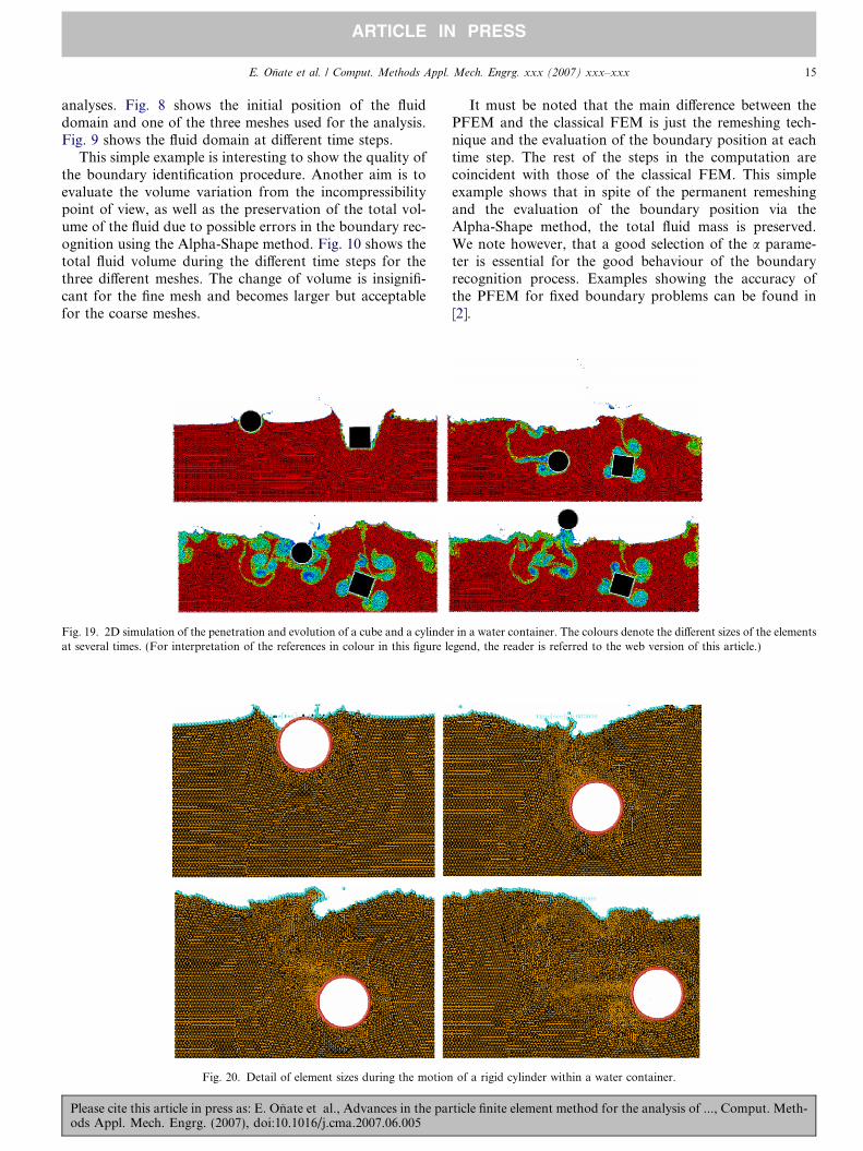
Fig. 20. Detail of element sizes during the motion

Fig. 19. 2D simulation of the penetration and evolution of a cube and a cylindeat several times. (For interpretation of the references in colour in this figure le


It must be noted that the main difference between thePFEM and the classical FEM is just the remeshing tech-nique and the evaluation of the boundary position at eachtime step. The rest of the steps in the computation arecoincident with those of the classical FEM. This simpleexample shows that in spite of the permanent remeshingand the evaluation of the boundary position via theAlpha-Shape method, the total fluid mass is preserved.We note however, that a good selection of the a parame-ter is essential for the good behaviour of the boundaryrecognition process. Examples showing the accuracy ofthe PFEM for fixed boundary problems can be found in[2].

of a rigid cylinder within a water container.

r in a water container. The colours denote the different sizes of the elementsgend, the reader is referred to the web version of this article.)



ARTICLE IN PRESS

6. Treatment of contact conditions in the PFEM

6.1. Contact between the fluid and a fixed boundary

The motion of the solid is governed by the action of thefluid flow forces induced by the pressure and the viscousstresses acting at the common boundary CFS, as mentionedabove.

The condition of prescribed velocities at the fixedboundaries in the PFEM are applied in strong form tothe boundary nodes. These nodes might belong to fixedexternal boundaries or to moving boundaries linked tothe interacting solids. Contact between the fluid particlesand the fixed boundaries is accounted for by the incom-pressibility condition which naturally prevents the fluid

nodes to penetrate into the solid boundaries (Fig. 11). Thissimple way to treat the fluid–wall contact at mesh genera-tion level is a distinct and attractive feature of the PFEMformulation.

6.2. Contact between solid–solid interfaces

The contact between two solid interfaces is simply trea-ted by introducing a layer of contact elements between the

Fig. 21. Evolution of a water column within a pri


two interacting solid interfaces. This layer is automatically

created during the mesh generation step by prescribing aminimum distance (hc) between two solid boundaries. Ifthe distance exceeds the minimum value (hc) then the gen-erated elements are treated as fluid elements. Otherwise theelements are treated as contact elements where a relation-ship between the tangential and normal forces and the cor-responding displacement is introduced so as to modelelastic and frictional contact effects in the normal and tan-gential directions, respectively (Fig. 12).

This algorithm has proven to be very effective and itallows to identifying and modeling complex frictional con-tact conditions between two or more interacting bodiesmoving in water in an extremely simple manner. Of coursethe accuracy of this contact model depends on the criticaldistance above mentioned.

This contact algorithm can also be used effectively tomodel frictional contact conditions between rigid or elasticsolids in standard structural mechanics applications. Figs.13–16 show examples of application of the contact algo-rithm to the bumping of a ball falling in a container, thefailure of a domino set, the failure of an arch formed bya collection of stone blocks under a seismic loading andthe motion of five tetrapods as they fall and slip over an

smatic container including a vertical cylinder.



ARTICLE IN PRESS

inclined plane, respectively. The images in Figs. 13 and 17show explicitly the layer of contact elements which controlsthe accuracy of the contact algorithm.

7. Modeling of bed erosion

Prediction of bed erosion and sediment transport inopen channel flows are important tasks in many areas ofriver and environmental engineering. Bed erosion can leadto instabilities of the river basin slopes. It can also under-mine the foundation of bridge piles thereby favouringstructural failure. Modeling of bed erosion is also relevantfor predicting the evolution of surface material dragged inearth dams in overspill situations. Bed erosion is one of themain causes of environmental damage in floods.

Bed erosion models are traditionally based on a rela-tionship between the rate of erosion and the shear stresslevel [14,33]. The effect of water velocity on soil erosionwas studied in [31]. In a recent work we have proposedan extension of the PFEM to model bed erosion [29].The erosion model is based on the frictional work at thebed surface originated by the shear stresses in the fluid.The resulting erosion model resembles Archard law typi-

Fig. 22. Impact of a wave on a prismatic co


cally used for modeling abrasive wear in surfaces underfrictional contact conditions [1,22].

The algorithm for modeling the erosion of soil/rock par-ticles at the fluid bed is the following:

1. Compute at every point of the bed surface the resultanttangential stress s induced by the fluid motion. In 3Dproblems s ¼ ðs2

s þ stÞ2 where ss and st are the tangentialstresses in the plane defined by the normal direction n atthe bed node. The value of s for 2D problems can beestimated as follows:

st ¼ lct; ð34aÞ

with

ct ¼1

2

ovt

on¼ vk

t

2hk; ð34bÞ

where vkt is the modulus of the tangential velocity at the

node k and hk is a prescribed distance along the normalof the bed node k. Typically hk is of the order of magni-tude of the smallest fluid element adjacent to node k

(Fig. 18).

lumn on a slab sustained by four pillars.


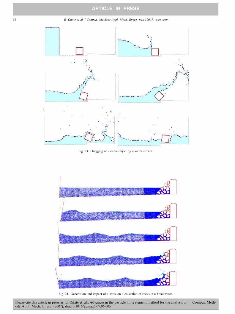
Fig. 23. Dragging of a cubic object by a water stream.

Fig. 24. Generation and impact of a wave on a collection of rocks in a breakwater.


ARTICLE IN PRESS

Please cite this article in press as: E. Onate et al., Advances in the particle finite element method for the analysis of ..., Comput. Meth-ods Appl. Mech. Engrg. (2007), doi:10.1016/j.cma.2007.06.005


ARTICLE IN PRESS

2. Compute the frictional work originated by the tangen-tial stresses at the bed surface as

W f ¼Z t

0

stct dt ¼Z t

0

l4

vkt

hk

� �2

dt: ð35Þ

Fig. 25. Detail of the impact of a wave on a breakwater. The arro

Fig. 26. 3D simulation of the impact of a wav


Eq. (35) is integrated in time using a simple scheme as

nW f ¼ n�1W f þ stctDt: ð36Þ3. The onset of erosion at a bed point occurs when nWf

exceeds a critical threshold value Wc defined empiricallyaccording to the specific properties of the bed material.

ws indicate the water force on the rocks at different instants.

e on a collection of rocks in a breakwater.



ARTICLE IN PRESS

4. If nWf > Wc at a bed node, then the node is detachedfrom the bed region and it is allowed to move with thefluid flow, i.e. it becomes a fluid node. As a consequence,

Fig. 27. Interaction of a wave with a vertical p

Fig. 28. Motion of two tetrapods


the mass of the patch of bed elements surrounding thebed node vanishes in the bed domain and it is trans-ferred to the new fluid node. This mass is subsequently

ier formed by reinforced concrete cylinders.

falling in a water container.



ARTICLE IN PRESS

transported with the fluid. Conservation of mass of thebed particles within the fluid is guaranteed by changingthe density of the new fluid node so that the mass of thesuspended sediment traveling with the fluid equals themass originally assigned to the bed node. Recall thatthe mass assigned to a node is computed by multiplyingthe node density by the tributary domain of the node.

5. Sediment deposition can be modeled by an inverse pro-cess to that described in the previous step. Hence, a sus-pended node adjacent to the bed surface with a velocitybelow a threshold value is assigned to the bed surface.This automatically leads to the generation of new bedelements adjacent to the boundary of the bed region.The original mass of the bed region is recovered byadjusting the density of the newly generated bedelements.

Fig. 18 shows an schematic view of the bed erosion algo-rithm proposed.

8. FSI examples

The examples chosen show the applicability of thePFEM to solve problems involving large motions ofthe free surface, fluid–multibody interactions and bederosion.

Fig. 29. Motion of 10 tetrapods on


8.1. Rigid objects falling into water

The analysis of the motion of submerged or floatingobjects in water is of great interest in many areas of har-bour and coastal engineering and naval architecture amongothers.

Fig. 19 shows the penetration and evolution of a cubeand a cylinder of rigid shape in a container with water.The colours denote the different sizes of the elements at sev-eral times. In order to increase the accuracy of the FSIproblem smaller size elements have been generated in thevicinity of the moving bodies during their motion (Fig. 20).

8.2. Impact of water streams on rigid structures

Fig. 21 shows an example of a wave breaking within aprismatic container including a vertical cylinder. Fig. 22shows the impact of a wave on a vertical column sustainedby four pillars. The objective of this example was to modelthe impact of a water stream on a bridge pier accountingfor the foundation effects.

8.3. Dragging of objects by water streams

Fig. 23 shows the effect of a wave impacting on a rigidcube representing a vehicle. This situation is typical in

a slope under an incident wave.


Fig. 30. Detail of the motion of 10 tetrapods on a slope under an incident wave. The figure shows the complex interactions between the water particles andthe tetrapods.


ARTICLE IN PRESS

flooding and Tsunami situations. Note the layer of contactelements modeling the frictional contact conditionsbetween the cube and the bottom surface.

8.4. Impact of sea waves on breakwaters and piers

Fig. 24 shows the 2D simulation of the impact of a wavegenerated in an experimental flume on a collection of rigidrocks representing a breakwater. Details of the water–rockinteraction are shown in Fig. 25.

Fig. 26 shows a 3D analysis of a similar problem. Fig. 27shows the 3D simulation of the interaction of a wave with avertical pier formed by a collection of reinforced concretecylinders.

The examples shown in Figs. 28 and 29 evidence thepotential of the PFEM to solve 3D problems involvingcomplex interactions between water and moving solidobjects. Fig. 28 shows the simulation of the falling of twotetrapods in a water container. Fig. 29 shows the motion


of a collection of ten tetrapods placed in a slope underan incident wave.

Fig. 30 shows a detail of the complex three-dimensionalinteractions between the water particles and the tetrapodsand between the tetrapods themselves, which can be easilymodeled with the PFEM.

8.5. Erosion of a 3D earth dam due to an overspill stream

We present finally a simple, schematic, but very illustra-tive example showing the potential of the PFEM to modelbed erosion in free surface flows.

The example represents the erosion of an earth damunder a water stream running over the dam top. A sche-matic geometry of the dam has been chosen to simplifythe computations. Sediment deposition is not consideredin the solution. The images of Fig. 31 show the progressiveerosion of the dam until the whole dam is dragged out bythe fluid flow.


Fig. 31. Erosion of a 3D earth dam due to an overspill stream.


ARTICLE IN PRESS

Other applications of the PFEM to bed erosion prob-lems can be found in [29].

9. Conclusions

The particle finite element method (PFEM) is ideal totreat problems involving fluids with free surfaces and sub-merged or floating structures and bodies within a unifiedLagrangian finite element framework. Problems such asfluid–structure interaction, large motion of fluid or solidparticles, surface waves, water splashing, separation ofwater drops, frictional contact situations between fluid–solid and solid–solid interfaces, bed erosion, etc. can beeasily solved with the PFEM. The success of the methodlies in the accurate and efficient solution of the equationsof an incompressible fluid and of solid dynamics using anupdated Lagrangian formulation and a stabilized finite ele-ment method, allowing the use of low order elements withequal order interpolation for all the variables. Other essen-tial solution ingredients are the efficient regeneration of thefinite element mesh using an extended Delaunay tessela-tion, the identification of the boundary nodes using anAlpha-Shape type technique and the simple algorithm totreat frictional contact conditions at fluid–solid andsolid–solid interfaces via mesh generation. The examplespresented have shown the great potential of the PFEMfor solving a wide class of practical FSI problems in engi-neering. Examples of validation of the PFEM results withdata from experimental tests are reported in [15].

Acknowledgements

Thanks are given to Mrs. M. de Mier for many usefulsuggestions. This research was partially supported by pro-


ject SEDUREC of the Consolider Programme of the Min-isterio de Educacion y Ciencia of Spain.

References

[1] J.F. Archard, Contact and rubbing of flat surfaces, J. Appl. Phys. 24(8) (1953) 981–988.

[2] R. Aubry, S.R. Idelsohn, E. Onate, Particle finite element method influid mechanics including thermal convection–diffusion, Comput.Struct. 83 (17–18) (2005) 1459–1475.

[3] R. Codina, O.C. Zienkiewicz, CBS versus GLS stabilization of theincompressible Navier–Stokes equations and the role of the time stepas stabilization parameter, Commun. Numer. Methods Engrg. 18 (2)(2002) 99–112.

[4] F. Del Pin, S.R. Idelsohn, E. Onate, R. Aubry, The ALE/Lagrangianparticle finite element method: a new approach to computation offree-surface flows and fluid–object interactions, Comput. Fluids 36(2007) 27–38.

[5] J. Donea, A. Huerta, Finite Element Method for Flow Problems,John Wiley, 2003.

[6] H. Edelsbrunner, E.P. Mucke, Three dimensional alpha shapes, ACMTrans. Graphics 13 (1999) 43–72.

[7] J. Garcıa, E. Onate, An unstructured finite element solver for shiphydrodynamic problems, J. Appl. Mech. 70 (2003) 18–26.

[8] S.R. Idelsohn, E. Onate, F. Del Pin, N. Calvo, Lagrangian formu-lation: the only way to solve some free-surface fluid mechanicsproblems, in: H.A. Mang, F.G. Rammerstorfer, J. Eberhardsteiner(Eds.), Fifth World Congress on Computational Mechanics, July 7–12, Vienna, Austria, 2002.

[9] S.R. Idelsohn, E. Onate, N. Calvo, F. Del Pin, The meshless finiteelement method, Int. J. Numer. Methods Engrg. 58 (6) (2003) 893–912.

[10] S.R. Idelsohn, E. Onate, F. Del Pin, A Lagrangian meshless finiteelement method applied to fluid–structure interaction problems,Comput. Struct. 81 (2003) 655–671.

[11] S.R. Idelsohn, N. Calvo, E. Onate, Polyhedrization of an arbitrarypoint set, Comput. Meth. Appl. Mech. Engrg. 192 (22–24) (2003)2649–2668.

[12] S.R. Idelsohn, E. Onate, F. Del Pin, The particle finite elementmethod: a powerful tool to solve incompressible flows with free-



ARTICLE IN PRESS

surfaces and breaking waves, Int. J. Numer. Methods Engrg. 61(2004) 964–989.

[13] S.R. Idelsohn, E. Onate, F. Del Pin, N. Calvo, Fluid–structureinteraction using the particle finite element method, Comput. Meth.Appl. Mech. Engrg. 195 (2006) 2100–2113.

[14] A. Kovacs, G. Parker, A new vectorial bedload formulation and itsapplication to the time evolution of straight river channels, J. FluidMech. 267 (1994) 153–183.

[15] L. Larese, R. Rossi, E. Onate, S.R. Idelsohn, Validation of theParticle Finite Element Method (PFEM) for simulation of freesurface flows, Engrg. Comput., submitted for publication.

[16] R. Ohayon, Fluid–structure interaction problem, in: E. Stein, R. deBorst, T.J.R. Hugues (Eds.), Encyclopedia of ComputationalMechanics, vol. 2, John Wiley, 2004, pp. 683–694.

[17] E. Onate, Derivation of stabilized equations for advective–diffusivetransport and fluid flow problems, Comput. Meth. Appl. Mech.Engrg. 151 (1998) 233–267.

[18] E. Onate, A stabilized finite element method for incompressibleviscous flows using a finite increment calculus formulation, Comput.Meth. Appl. Mech. Engrg. 182 (1–2) (2000) 355–370.

[19] E. Onate, Possibilities of finite calculus in computational mechanics,Int. J. Numer. Methods Engrg. 60 (1) (2004) 255–281.

[20] E. Onate, S.R. Idelsohn, A mesh free finite point method foradvective–diffusive transport and fluid flow problems, Comput.Mech. 21 (1998) 283–292.

[21] E. Onate, J. Garcıa, A finite element method for fluid–structureinteraction with surface waves using a finite calculus formulation,Comput. Meth. Appl. Mech. Engrg. 191 (2001) 635–660.

[22] E. Onate, J. Rojek, Combination of discrete element and finiteelement method for dynamic analysis of geomechanic problems,Comput. Meth. Appl. Mech. Engrg. 193 (2004) 3087–3128.

[23] E. Onate, C. Sacco, S.R. Idelsohn, A finite point method forincompressible flow problems, Comput. Visual. Sci. 2 (2000) 67–75.

[24] E. Onate, S.R. Idelsohn, F. Del Pin, Lagrangian formulation forincompressible fluids using finite calculus and the finite element


method, in: Y. Kuznetsov, P. Neittanmaki, O. Pironneau (Eds.),Numerical Methods for Scientific Computing Variational Problemsand Applications, CIMNE, Barcelona, 2003.

[25] E. Onate, J. Garcıa, S.R. Idelsohn, Ship hydrodynamics, in: E. Stein,R. de Borst, T.J.R. Hughes (Eds.), Encyclopedia of ComputationalMechanics, vol. 3, John Wiley, 2004, pp. 579–610.

[26] E. Onate, S.R. Idelsohn, F. Del Pin, R. Aubry, The particle finiteelement method. An overview, Int. J. Comput. Methods 1 (2) (2004)267–307.

[27] E. Onate, A. Valls, J. Garcıa, FIC/FEM formulation with matrixstabilizing terms for incompressible flows at low and high Reynold’snumbers, Comput. Mech. 38 (4–5) (2006) 440–455.

[28] E. Onate, J. Garcıa, S.R. Idelsohn, F. Del Pin, FIC formulations forfinite element analysis of incompressible flows. Eulerian, ALE andLagrangian approaches, Comput. Meth. Appl. Mech. Engrg. 195 (23–24) (2006) 3001–3037.

[29] E. Onate, M.A. Celigueta, S.R. Idelsohn, Modeling bed erosion infree surface flows by the Particle Finite Element Method, ActaGeotechnia 1 (4) (2006) 237–252.

[30] E. Onate, S.R. Idelsohn, R. Rossi, Enhanced FIC–FEM formulationfor incompressible flows, Research Report, CIMNE Barcelona,March, 2007.

[31] D.B. Parker, T.G. Michel, J.L. Smith, Compaction and water velocityeffects on soil erosion in shallow flow, J. Irrigation Drainage Engrg.121 (1995) 170–178.

[32] T.E. Tezduyar, Finite element method for fluid dynamics with movingboundaries and interface, in: E. Stein, R. de Borst, T.J.R. Hugues(Eds.), Encyclopedia of Computational Mechanics, vol. 3, JohnWiley, 2004, pp. 545–578.

[33] C.F. Wan, R. Fell, Investigation of erosion of soils in embankmentdams, J. Geotechn. Geoenviron. Engrg. 130 (2004) 373–380.

[34] O.C. Zienkiewicz, R.L. Taylor, P. Nithiarasu, The Finite ElementMethod for Fluid Dynamics, Elsevier, 2006.

[35] O.C. Zienkiewicz, R.L. Taylor, The Finite Element Method for Solidand Structural Mechanics, Elsevier, 2005.


advances in the particle ﬁnite element method for the ... · description and the fic formulation...

Documents