advantages and challenges of programming the micron automata
TRANSCRIPT
Iowa State UniversityDigital Repository @ Iowa State University
Graduate Theses and Dissertations Graduate College
2013
Advantages and challenges of programming theMicron Automata ProcessorChristopher SabottaIowa State University, [email protected]
Follow this and additional works at: http://lib.dr.iastate.edu/etdPart of the Computer Engineering Commons
This Thesis is brought to you for free and open access by the Graduate College at Digital Repository @ Iowa State University. It has been accepted forinclusion in Graduate Theses and Dissertations by an authorized administrator of Digital Repository @ Iowa State University. For more information,please contact [email protected].
Recommended CitationSabotta, Christopher, "Advantages and challenges of programming the Micron Automata Processor" (2013). Graduate Theses andDissertations. Paper 13613.
Advantages and challenges of programming the Micron Automata Processor
by
Christopher R. Sabotta
A thesis submitted to the graduate faculty
in partial fulfillment of the requirements for the degree of
MASTER OF SCIENCE
Major: Computer Engineering
Program of Study Committee:Srinivas Aluru, Major Professor
Chris ChuAkhilesh Tyagi
Iowa State University
Ames, Iowa
2013
Copyright c© Christopher R. Sabotta, 2013. All rights reserved.

ii
DEDICATION
I would like to dedicate this thesis to my family. Their unconditional care for me has been
at the heart of all my accomplishments.
I would also like to thank my friends for their care and support during the writing of this work.

iii
TABLE OF CONTENTS
LIST OF TABLES . . . . . . . . . . . . . . . . . . . . . . . . . . . . . . . . . . . iv
LIST OF FIGURES . . . . . . . . . . . . . . . . . . . . . . . . . . . . . . . . . . v
ACKNOWLEDGEMENTS . . . . . . . . . . . . . . . . . . . . . . . . . . . . . . vi
ABSTRACT . . . . . . . . . . . . . . . . . . . . . . . . . . . . . . . . . . . . . . . vii
CHAPTER 1 INTRODUCTION . . . . . . . . . . . . . . . . . . . . . . . . . 1
CHAPTER 2 UNDERSTANDING THE MICRON AUTOMATA PRO-
CESSOR . . . . . . . . . . . . . . . . . . . . . . . . . . . . . . . . . . . . . . . 4
2.1 Introduction . . . . . . . . . . . . . . . . . . . . . . . . . . . . . . . . . . . . . . 4
2.2 Understanding the Automata Processor . . . . . . . . . . . . . . . . . . . . . . 4
2.2.1 Sequential processor implementations of NFA . . . . . . . . . . . . . . . 4
2.2.2 Automata Processor implemenations of NFA . . . . . . . . . . . . . . . 5
2.2.3 Gaining parallelism . . . . . . . . . . . . . . . . . . . . . . . . . . . . . . 6
2.3 Automata Processor implementation . . . . . . . . . . . . . . . . . . . . . . . . 7
2.4 Competing NFA hardware . . . . . . . . . . . . . . . . . . . . . . . . . . . . . . 8
2.4.1 Scope of ability . . . . . . . . . . . . . . . . . . . . . . . . . . . . . . . . 8
2.4.2 Performance and capacity . . . . . . . . . . . . . . . . . . . . . . . . . . 8
CHAPTER 3 USING THE MICRON AUTOMATA PROCESSOR . . . . 11
3.1 Automata Processor components . . . . . . . . . . . . . . . . . . . . . . . . . . 11
3.1.1 Types of element . . . . . . . . . . . . . . . . . . . . . . . . . . . . . . . 12
3.1.2 Input and output . . . . . . . . . . . . . . . . . . . . . . . . . . . . . . . 14
3.2 Modeling automata . . . . . . . . . . . . . . . . . . . . . . . . . . . . . . . . . . 14

iv
3.2.1 Using Automata Network Markup Language . . . . . . . . . . . . . . . 15
CHAPTER 4 SCANNING FOR PROTEIN MOTIFS USING THE MI-
CRON AUTOMATA PROCESSOR . . . . . . . . . . . . . . . . . . . . . . 18
4.1 abstract . . . . . . . . . . . . . . . . . . . . . . . . . . . . . . . . . . . . . . . . 18
4.2 Introduction . . . . . . . . . . . . . . . . . . . . . . . . . . . . . . . . . . . . . . 19
4.3 Methodology . . . . . . . . . . . . . . . . . . . . . . . . . . . . . . . . . . . . . 20
4.3.1 PROSITE patterns . . . . . . . . . . . . . . . . . . . . . . . . . . . . . . 21
4.3.2 Conversion of PROSITE patterns to ANML automata . . . . . . . . . . 22
4.3.3 Finding patterns in proteins . . . . . . . . . . . . . . . . . . . . . . . . . 25
4.3.4 Finding pattern locations in proteins . . . . . . . . . . . . . . . . . . . . 26
4.4 Implementation and results . . . . . . . . . . . . . . . . . . . . . . . . . . . . . 26
4.4.1 Compile-time overhead . . . . . . . . . . . . . . . . . . . . . . . . . . . . 26
4.4.2 Execution-time overhead . . . . . . . . . . . . . . . . . . . . . . . . . . . 27
4.4.3 Effective processing rate . . . . . . . . . . . . . . . . . . . . . . . . . . . 28
4.4.4 Comparison and results . . . . . . . . . . . . . . . . . . . . . . . . . . . 28
4.5 Conclusion . . . . . . . . . . . . . . . . . . . . . . . . . . . . . . . . . . . . . . 29
CHAPTER 5 APPLICATION DEVELOPERS’ NOTES . . . . . . . . . . . 31
5.1 Automata Processor Board configuration . . . . . . . . . . . . . . . . . . . . . . 31
5.2 Finer details for designing automata . . . . . . . . . . . . . . . . . . . . . . . . 32
5.2.1 Element and routing implementation . . . . . . . . . . . . . . . . . . . . 32
5.2.2 Avoiding scaling and routing pitfalls . . . . . . . . . . . . . . . . . . . . 33
5.3 Designing robust solutions . . . . . . . . . . . . . . . . . . . . . . . . . . . . . . 35
5.3.1 Multiple automata instances . . . . . . . . . . . . . . . . . . . . . . . . 35
5.3.2 Managing input and output data . . . . . . . . . . . . . . . . . . . . . . 37
CHAPTER 6 CONCLUSION . . . . . . . . . . . . . . . . . . . . . . . . . . . 40

v
LIST OF TABLES
2.1 Processing and Storage Complexity for NFA Implementation . . . . . . 6
4.1 Total Computation Time for Sample Problem Instances (s) . . . . . . 28
vi
LIST OF FIGURES
Figure 2.1 Automata exhibiting dual parallelism . . . . . . . . . . . . . . . . . . . 7
Figure 3.1 Counting machine using exclusively STEs . . . . . . . . . . . . . . . . 13
Figure 3.2 Counting machine using a Counter Element . . . . . . . . . . . . . . . 13
Figure 4.1 Overview of the working of PROTOMATA . . . . . . . . . . . . . . . . 21
Figure 4.2 The filter-automaton. . . . . . . . . . . . . . . . . . . . . . . . . . . . . 24
Figure 4.3 The location-automaton . . . . . . . . . . . . . . . . . . . . . . . . . . 25
Figure 4.4 Protomata Scaling Efficiency . . . . . . . . . . . . . . . . . . . . . . . . 29
Figure 5.1 Genome mapping tree solution . . . . . . . . . . . . . . . . . . . . . . . 34
Figure 5.2 Genome mapping decomposed solution . . . . . . . . . . . . . . . . . . 35
Figure 5.3 Automata redefined without additional compilation . . . . . . . . . . . 38

vii
ACKNOWLEDGEMENTS
I would like to take this opportunity to thank those who helped me with the research and
writing of this thesis.
First and foremost, Dr. Srinivas Aluru for his inspiration, teaching and support throughout
the development of this work, even when at a distance. I appreciate him accepting me as a
student and I am thankful for what he has taught me.
I would also like to thank my committee members for their support of this work: Dr. Chris
Chu and Dr. Akhilesh Tyagi.
I would like to sincerely thank Indranil Roy for his contributions and insight throughout the
entire duration of the project. Indranil has been exceptionally teaching and patient with all of
his help and I am truly grateful.
I am thankful for Micron for sponsoring my research, and for providing me with the resources
and opportunities I needed.
I would also like to thank Michael Leventhal, Matt Tanner, and all of their colleagues at Micron
for their assistance. Their persistent communication and collaboration has been essential.
viii
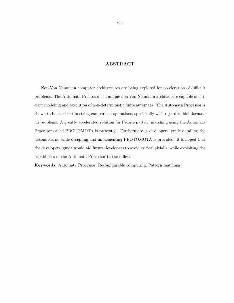
ABSTRACT
Non-Von Neumann computer architectures are being explored for acceleration of difficult
problems. The Automata Processor is a unique non Von Neumann architecture capable of effi-
cient modeling and execution of non-deterministic finite automata. The Automata Processor is
shown to be excellent in string comparison operations, specifically with regard to bioinformat-
ics problems. A greatly accelerated solution for Prosite pattern matching using the Automata
Processor called PROTOMOTA is presented. Furthermore, a developers’ guide detailing the
lessons learnt while designing and implementing PROTOMOTA is provided. It is hoped that
the developers’ guide would aid future developers to avoid critical pitfalls, while exploiting the
capabilities of the Automata Processor to the fullest.
Keywords: Automata Processor, Reconfigurable computing, Pattern matching.
1
CHAPTER 1 INTRODUCTION
Today, a lot is known about the world around us. Ironically, relatively little is known about
what governs what is going on inside us. This has been changing of late with the continued
introduction of extremely fast and increasingly accurate biological instruments and computing
methods which has enabled the field of biology to grow in ways that might otherwise been
impossible. It is the combination of this computer engineering and biology which brings us
now the study of bioinformatics, perhaps one of the most prolific fields of the twenty-first
century.
Many important bioinformatics problems are complex and often take a lot of time and
resources. In order to truly extend our knowledge in this field, efficient solutions to these
problems need to be developed so that many instances of the problem can be solved providing
the necessary insight to understand the underlying biology. Therefore we need to accelerate
the processes. Many researchers are looking at accelerating these using Von Neumann archi-
tectures like multicore, many core systems, GPUs etc. This thesis examines whether certain
problems could be better solved using a novel non-Von Neumann architecture called the Micron
Automata Processor.
Conventional computer processors are extremely quick at performing individual operations
in linear succession. With these CPUs billions of individual commands can be executed one af-
ter another every second. Unfortunately, solutions of many problems in bioinformatics contain
a high density of conditional branching, wherein even this seemingly fast processor can take
unacceptable amounts of time to find the result. Non-deterministic Finite Automata (NFA) is
an intuitive mechanism for modeling such problems, but the author is unaware of any hardware
architecture which can directly execute parallel paths in an NFA concurrently. In CPU based

2
architectures, execution of an NFA may lead to a state-space explosion leading to exponential
run-time complexity.
The Automata Processor (AP) is the first semiconductor device where the execution of an
NFA can be directly emulated on the device. Besides, the large capacity of the processor allows
the execution of many NFAs in parallel, leading to large scale speedup. Thus the Automata
Processor can work as an effective accelerator for many applications in bioinformatics.
An intuitive use of the Automata Processor is to aid in the characterization of protein
sequences through the identification of motif-patterns present in them. Prosite is a large an-
notated database of known protein motifs. These motifs are represented either as patterns
defined using a syntax very similar to that of regular expressions or on Hidden Markov Model
based profiles. In the rest of this document we would only be considering only motifs expressed
as patterns in the database, of which there are currently 1308 entries. Each of these patterns
are converted into an automaton and defined using the Automata Network Markup Language
(ANML, pronounced as ANiMaL) in order to enable their execution on the Automata Pro-
cessor. After the automata are loaded onto the Automata Processor, the protein sequence(s)
are streamed to check for the occurrence of any motifs in them. The occurrence of a motif
is signaled by the reaching of an accept state of the corresponding automaton. The ending
position of the occurance of the motif in a protein sequence is marked by offset in the protein
sequence when the accept state was matched. The large capacity of the Automata Processor
allows the automata for the entire database of Prosite patterns to be loaded on a single chip
simultaneously. By executing all the atomata concurrently, large speedups can be obtained.
It goes without saying that the Automata Processor is a unique device. Utilizing the
power of the Automata Processor means modeling solutions to problems in unconventional
ways. Even skilled developers may initially find it challenging to think of solutions in terms
of NFA. Besides, the developers need to learn the nuances of using this device effectively and
the restrictions that it places on the automata for their efficient execution. In this thesis,
the Developers Note section contains all the lessons learnt while designing and implementing
PROTOMOTA. This section details the discovered brilliance and pitfalls of developing for the
3
Automata Processor and seeks to lower the barriers of entry to programming on the Automata
Processor.
Although adjusting to the novelty of the Automata Processor was at times arduous, it
proved to be rewarding. The implementation of the PROSITE patterns in the Automata
Processor is intuitive, and the acceleration provided is exemplary. For such direct, regular-
expression-like string matching the Automata Processor seems unparalleled. The Automata
Processor stands to show itself as an impressive boon for the world of bioinformatics and will
be watched with anticipation as future generations of it are developed.
The rest of this thesis is organized as follows. First, chapter 2 provides an introduction
to the Automata Processor. Further, chapter 3 then discusses programming model and ways
of programming the automta processor. In chapter 4, an application to accelerate the search
for motif-patterns in protein sequences using the Automata Processor called PROTOMATA is
presented. This is followed by the detailed developers’ notes in Chapter 5. Finally, this thesis
culminated with conclusion and scope of future work in Chapter 6.

4
CHAPTER 2 UNDERSTANDING THE MICRON AUTOMATA
PROCESSOR
2.1 Introduction
The Micron Automata Processor (AP) is a highly parallel reconfigurable non-von Neu-
mann architecture designed for the emulation of Non-Deterministic Finite Automata (NFA).
The Automata Processor is effective in modeling complex regular expressions as well as other
more complex automata. The architecture allows for effective solutions for pattern match-
ing problems found in computational biology, cyber security, graphics processing, and more.
Its purpose-built design exceeds the capabilities of similar FPGA-based solutions while also
significantly outperforming them. The Automata Processor connects to a system through
PCI Express and is designed to supplement a CPU as an acceleration device rather than a
standalone utility.
2.2 Understanding the Automata Processor
The Automata Processor is purpose-built hardware designed specifically for the acceleration
of processing Non-Deterministic Finite Automata (NFA). The processing of NFA has become
an important topic as they offer an intuitive model for regular expression matching problems,
which can be extended to numerous fields.
2.2.1 Sequential processor implementations of NFA
A von Nuemann sequential processor (CPU) may take a direct approach of modeling an
NFA by defining a set of states and connections. By maintaining a list of which states are
active, and given the next token of input data, the next set of states can be computed and
5
updated. Unfortunately, the CPU must make considerations for each of its active states and
their connections sequentially, and such state processing time is increased with increased ac-
tivity across the graph. In the worst case, the entire NFA may be active resulting in the entire
graph needing to be considered for a given character of input - yielding a processing complexity
O(n2). Although such direct solutions offer a simple storage cost O(n), the large processing
complexity makes them unrealistic for large problems.
While CPUs struggle with the processing of multiple simultaneous states in NFA, Deter-
ministic Finite Automata (DFA) require singularity in state. This property allows for the
direct processing O(1) of DFA, and encourages a translation from NFA to DFA. For an NFA
to be modeled as a DFA, the equivalent DFA must be able to model any combination of si-
multaneous states possible in the NFA. For this reason while NFA can be reliably converted
into equivalent DFA [2], it comes with the challenge of significantly inceased storage cost.
The storage cost reduction of NFA-derived DFA is the target of much research, and has
been viewed from many different perpectives. Some solutions such as Campeanu et al. [3]
focus on simplifying the NFA as much as possible by combining excessive states. Other solu-
tions attempt to reduce the scope of the problem to allow for simplifications. Chia-Hsiang et
al. [4] require compressed NFA specifically taken from regular expressions for their solution.
Alternately, Holub [13] attempts storage and simulation simplifications through dynamic pro-
gramming. While many unique solutions have been developed however, no solution escapes
the exponential DFA storage cost. [25, 24, 23, 21]
2.2.2 Automata Processor implemenations of NFA
The Automata Processor allows for a physical implementation of NFA. It has many con-
figurable elements which act as individual states for a modeled NFA. These elements can be
dynamically connected to one another and configured to respond to different stimuli. In this
way the Automata Processor is capable of literally modeling NFA directly. Because of this the
Automata Processor has a direct NFA storage cost of O(n).
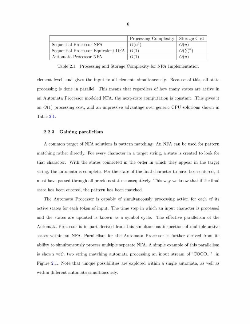
The physical design of the Automata Processor allows for processing to be done at an
6
Processing Complexity Storage Cost
Sequential Processor NFA O(n2) O(n)
Sequential Processor Equivalent DFA O(1) O(∑n)
Automata Processor NFA O(1) O(n)
Table 2.1 Processing and Storage Complexity for NFA Implementation
element level, and gives the input to all elements simultaneously. Because of this, all state
processing is done in parallel. This means that regardless of how many states are active in
an Automata Processor modeled NFA, the next-state computation is constant. This gives it
an O(1) processing cost, and an impressive advantage over generic CPU solutions shown in
Table 2.1.
2.2.3 Gaining parallelism
A common target of NFA solutions is pattern matching. An NFA can be used for pattern
matching rather directly. For every character in a target string, a state is created to look for
that character. With the states connected in the order in which they appear in the target
string, the automata is complete. For the state of the final character to have been entered, it
must have passed through all previous states consequtively. This way we know that if the final
state has been entered, the pattern has been matched.
The Automata Processor is capable of simultaneously processing action for each of its
active states for each token of input. The time step in which an input character is processed
and the states are updated is known as a symbol cycle. The effective parallelism of the
Automata Processor is in part derived from this simultaneous inspection of multiple active
states within an NFA. Parallelism for the Automata Processor is further derived from its
ability to simultaneously process multiple separate NFA. A simple example of this parallelism
is shown with two string matching automata processing an input stream of ’COCO...’ in
Figure 2.1. Note that unique possibilities are explored within a single automata, as well as
within different automata simultaneously.

7
Figure 2.1 Automata exhibiting dual parallelism
2.3 Automata Processor implementation
The entire Automata Processor exists as a conglomeration of 6 distinct ranks connected to
a system through PCI Express. An Automata Processor rank consists of 8 distinct Automata
Processor cores on a single chip. Each core consists of two half-cores containing 24K elements
each, where no connections can be made between elements of unique half-cores. It is the
elements of these half-cores which are used to directly model the states of NFA.
With a section of the Automata Processor configured to model a desired NFA, input can be
streamed. The modeled NFA views each streamed-in character as the stimulus for a potential
state transition. An Automata Processor core processes data at a rate of 1 Gbps. Because
one byte characters are the fundamental unit of the Automata Processor this can be better
viewed as 128 ∗ 106 characters per second. This means that the state of a modeled NFA can
be updated every 7.45 ∗ 10−9s. This time is also known as a symbol cycle.
Cores can be associated among their rank, in groups of 1, 2, 4, 8 cores. Grouped cores will
receive data from the same stream of data, while cores of different groups can concurrently
process different streams of data. With all cores associated in one group of 8 the Automata
Processor has an effective throughput of 1 Gbps. With all cores grouped individually with
their own data streams an effective throughput of 8 Gbps is achieved.

8
2.4 Competing NFA hardware
While NFA are difficult to emulate with a sequential processor, Field Programmable Gate
Arrays (FPGAs) are capable of NFA modeling with the use of look up tables [24, 23, 21]. Sim-
ilarly, GPU based solutions have been devised [25]. Due to its specialization, the Automata
Processor is able to show decisive advantage over such FPGA and GPU based solutions. Fur-
thermore, the Automata Processor remains the only such specialized non-FPGA, non-GPU
hardware.
2.4.1 Scope of ability
FPGA and GPU based competing NFA solutions focus directly on implemenation of Perl
Compatible Regular Expressions (PCRE)[1]. For the sake of direct comparison, the Automata
Processor is assessed in terms of such regular expressions. It is important to note however
that the Automata Processor maintains the unique ability to model non-PCRE NFA through
its own configuration language. This configuration language is known as Automata Network
Markup Language (ANML) and allows for simple directed implementation of NFAs with an
XML structure.
The Automata Processor uniquely allows for scaling across multiple chips with balancing
for capacity and throughput. The architecture also allows for new automata to be added to
dynamically to the chip without recompiling the existing automata. This process is known
as incremental update and is only possible with the Automata Processor, whereas competing
FPGA and GPU solutions require a new compilation [25, 23, 21, 25]. Similarly, the Automata
Processor allows for the dynamic reconfiguration of match values and path pruning without re-
producing the layout of the chip. Outside of the Automata Processor, dynamic reconfiguration
is only present in competing solutions using restricted RegEx [8].
2.4.2 Performance and capacity
Although there are 6 ranks in one instance of the Automata Processor, because they cannot
cooperate only 1 rank is used for comparison against other solutions. While statistics on
9
throughput and capacity could be realistically increased by a factor of 6 in most cases, multiple
instances of other solutions could be used to the same effect. Still, the Automata Processor
maintains the advantage of being able to connect these 6 ranks to the rest of a system through
only a singular PCI Express port.
The Automata Processor is shown to be competitive with FPGA based solutions [24, 23, 21]
in terms of throughput. Raw comparisons of throughput are difficult to produce for a number
of reasons. First, various FPGA solutions show data consumption rates ranging anywhere
from 1 to 8 characters per cycle. While this increases the technical throughput, it does not
necessarily model the rate at which the NFA can transition between states. It must also be
considered however that larger per-cycle data consumption potentially introduces a higher
level of control. Wang et al. [23] boast a derived 2.57Gbps throughput but offer significantly
lower capacity than the Automata Processor, requiring 6 chips to fit roughly half the capacity
of an Automata Processor rank. Yang et al. [24] are capable of a 10Gpbs result, but this is
with a consumption of 8 characters per cycle. With slightly better efficiency they also present
a 3.5Gbps result consuming 2 characters per cycle, though all solutions present significantly
lower capacity than the Automata Processor at less than one fourth of one rank.
Competing GPU based solutions in that of Zu et al. [25] show results as high as nearly
14Gbps. In exchange for this rapid processing both routing an capacity are found to be
significantly weaker than with the Automata Processor. This GPU solution only allows for
4 connections from each element, where the Automata Processor allows for 16. Furthermore
the GPU solution can support only one sixth of the elements of a rank of the Automata
Processor. Although the GPU solution boasts a slightly higher throughput, multiple ranks of
the Automata Processor can match such throughput much more quickly than multiple instances
of the GPU can match the Automata Processors capacity. Even with matched capacity, the
Automata Processor remains superior in routing.
A rank of the Automata Processor is capable of producing up to 8Gbps throughput if
the problem can be dissolved into 8 unique streams. For large automata that must span
multiple cores and require the same input, the effective throughput is reduced relative to the
10
group size. This notion of chip scaling makes definative throughput comparisons difficult.
Though the Automata Processor cannot be determined to have higher throughput than all
GPU and FPGA solutions in all cases, it is shown to be competitive. For more infomation on
the comparative capabilities of the Automata Processor view Supplementary Material for An
Efficient and Scalable Semiconductor Architecture for Parallel Automata Processing [8]

11
CHAPTER 3 USING THE MICRON AUTOMATA PROCESSOR
The Automata Processor proves to be exceptionally effective for NFA implementation on
account of its reconfigurability and unique modeling capabilities. To fully utilize the strengths
of the Automata Processor its components and automata definition mechanisms must be un-
derstood. This chapter begins by defining the building blocks of Automata Processor NFA,
and continues to explain how such NFA can be programmed into the device.
3.1 Automata Processor components
The definition of NFA using the Automata Processor can be divided into two major com-
ponents: elements and connections. Individual states of NFA can be modeled using Automata
Processor elements. The directional connections between states are modeled by defining rout-
ing characteristics for these elements. Finally, input and output characteristics can be defined
for the automata are defined to complete a solution.
Elements of an automata can be either active or inactive at any given time. An active
element models an active state within the modeled automata. For each input character in the
stream whether or a not a state is active is determined by the following two queries:
1. The given element is on the receiving end of a connection with a currently active element
2. The given element is configured to accept or match the given input character
If both of these queries are true, the given element enters an active state for the next
processed input character. If either or both of these queries are false, the given element enters
an inactive state, regardless of its current state as a default action. Any element may become
12
permanently active after it is first activated. This process is known as latching. If an element
is in an active state, it is said to be driving any elements to which it connects.
3.1.1 Types of element
Elements provide the building blocks for any graph modeled by the Automata Processor.
Some elements are used for modeling state, while other elements exist for extended capabilities
such as basic logic and counting. Each type of element has unique configurable properties for
NFA modeling.
3.1.1.1 State transition element
The state transition element (STE) is the fundamental component of the automata. Each
STE holds a configurable symbol set which defines its matching characteristics. This symbol
set can be defined to be any subset contained within the full set of 256 possible input characters.
An STE directly models an NFA state and is processed for each character of input in what is
known as a symbol cycle. It is by far the most plentiful and most important type of element
for the Automata Processor.
3.1.1.2 Counter element
Counter elements serve to supplement the work of STEs, and add higher levels of modeling
capability to the Automata Processor. The counter element does not define a symbol set, nor
any other form of direct comparison. Instead, counter elements activate when a configurable
count is reached. Counter elements update an internal counter by one during each symbol cycle
they are driven by an active element. When the defined target is reached, the counter drives
its outgoing connections. This output driving can be configured to be either for a single pulse
or a latched, continuous operation. Counter elements also define an input port for resetting
the count. If a connection is driven to the reset port the count is returned to its original value.
Finally, it is important to note that counter elements driven by STEs are processed in the
same symbol cycle as the driving STE.
13
The counter element can be used to consolidate a large number of duplicate states. An
example is given showing two implementations for an automata designed to find 5 occurrences
of the character ’A’ before a final character ’B’. Figure 3.1 shows a solution with exclusively
STEs. Figure 3.2 shows a solution using the counter element.
Figure 3.1 Counting machine using exclusively STEs
Figure 3.2 Counting machine using a Counter Element
3.1.1.3 Logical element
The final class of element for constructing graphs on the Automata Processor is the logical
element. A logical element is similar to a counter element in that its action is determined by
input signals, and it is processed in the same symbol cycle as the STEs which drive it. Logical
elements are configured to view a series of incoming connections as a set of Boolean variables.
If a signal is being driven, it is considered to be a 1, and if it is not actively being driven
it is considered to be 0. The variable representation of these signals are then considered as
a programmable digital logic expression. The logical element is capable of simulating basic
AND, OR, NAND and NOR gates as well as Sum of Product (SoP) and Product of Sum (PoS)
expressions. Given a set of input signals and its programmed logic, output signals can be
14
driven based on the result.
3.1.2 Input and output
After defining the core implementation of an NFA, its beginning and ending states must be
considered. At the beginning of each problem instance for an Automata Processor solution, the
automata has no active states. Because the activation of further states is dependent on being
driven by currently active states, designated elements configured with the start property are
required. If an element is a startelement it is considered to be driven by the data stream, and
does not require being driven by another element. This start characteristic can be specified
either for only the first character of the data stream, or for all character of the data stream.
Output can be generated as a result of entering a designated state. If an element is
configured to generate output upon its activation the element is said to be reporting. A
reporting element can be configured to generate output data immediately upon its activation.
Alternately, a reporting element can be configured to wait until the end of the data stream and
report if it had been activated. A word of report data consists of the element which reported
it as well as the cycle in which the data has been matched. Current implementations of the
Automata Processor suffer large time penalties for repeated quick reporting. Unfortunately if
an element does not report until the end of data the knowledge of the matching symbol cycle
is lost. A quality Automata Processor solution will reasonably balance the use of reporting
elements.
3.2 Modeling automata
Programmed place and route executable solutions for the Automata Processor exist in
uniquely defined finite state machine (.fsm) automata files. Such solutions can be generated
in one of two ways using the Automata Processor compiler. 1) Regular Expressions can be
directly converted into programmable automata, or 2) Automata may be directly defined (and
go beyond regular expressions) with the XML based Automata Network Markup Language
(ANML). Generating automata directly from regular expressions is trivial, however it is very

15
limiting in terms of its capabilities. For this reason the remainder of this section focuses on the
implementation of automata using ANML. Although the general form of ANML is discussed, it
is important to review the most recent schema for the most up-to-date syntax and component
definition information.
3.2.1 Using Automata Network Markup Language
The Automata Network Markup Language (ANML, pronounced ANiMaL) provides a sim-
ple yet comprehensive language for describing automata in the vein of XML. ANML serves to
define elements and their connections within the scope of an automata network. Start and re-
porting characteristics as well as potential latching and other configurable aspects of elements
can be defined for each defined component. ANML also offers the notion of a macro for the
compartmentalization of sub graphs as well as simple reuse of functional graph components.
3.2.1.1 ANML XML layout
All specifications in ANML are made within matched XML tags. All defined components
of an automata must be described between matched automata-network tags. Beyond this
the definitions may be totally flat. The only other requirement for an ANML file is that all
components are given a unique id in their opening tag.
Individual elements can be defined using their appropriate definition tags. For each kind
of element there are both required fields and optional fields. Specifications for start, reporting,
latching and other optional behavior are not required and will use a simple default if unspecified.
Intrinsic properties of each element are required and will not compile if left undefined. STEs
must define a symbol set, Counter elements must specify a target, and logical elements must
specify a logical configuration.
Within the definition of an element, outgoing connections to other elements can be defined.
For this the activate-on-match tag is used in combination with the unique id of the target
element. With this basic understanding of element definition and connection specification,
fully functional NFA can be defined.
16
3.2.1.2 Using macros
Macro are an effective means for reproducing multiple identical or near identical sub graphs
without dramatically expanding the defining ANML. Macros may also be useful for adding a
level of organization to an automata by encapsulating complicated subgraphs into a high level
block.
As with other ANML components, macro definitions require a unique id for reference.
A macro definition is divided into two components labeled port definition and macro body.
The port definition is used to characterize the quantity and labels of incoming and outgoing
ports for the macro. Within the macro body internal elements are defined and connected.
Also within this macro body, a port mappings tag is used to connect internal elements to the
predefined ports.
Variables can be introduced into a macro definition for producing unique macro references
from the same definition. To accomplish this a parameter declaration field is added to the port
definition section of the macro definition. Within this parameter declaration parameter names
are defined with default values. These parameters are referenced within the macro body to
allow for variability.
Macro references generate instances of a specified macro definition. Macro references re-
quire their own unique id, as well as a use field specifying the target macro definition. If the
target macro definition has parameters, they must be specified by the macro reference or they
are returned to their default values. Connections using macro references can be named by
using name of the macro reference followed by the desired port.
3.2.1.3 Generating ANML
While the modeling of NFA in ANML is straightforward and relatively simple it can be
difficult to do for sizable solutions. Large and complicated graphs can be particularly difficult
to visualize and debug when simply read from a file. To avoid the difficulties of directly coding
ANML there are two main classes of abstraction: 1) Develop ANML in a graphical, drag and
drop environment or 2) Develop ANML through specialized executable programs.
17
The AP Workbench has been developed as the pioneer drag and drop graphical environment
for the formation of ANML files. It allows for rapid development of small automata, guarantees
valid syntax, and requires no formal understanding of ANML whatsoever. It is capable of
compiling and simulating its own ANML on the fly and allows for a comprehensive active
visual debugging. Unfortunately such graphical applications lack the ability to realistically
produce and simulate large applications.
Specialized executable programs offer a powerful alternative to graphical solutions. By
using other compiled languages to generate ANML, automata can be generated dynamically
with exceptional finesse based on some input parameters. Such an approach lends itself to
large, complicated, and automated solutions. Currently, no supporting libraries or API have
been released in any such languages. While such conversion applications can be effective,
they require significant development work and do not offer the same conveniences of graphical
development environments.
For large, complicated, variable automata development ANML conversion scripts or ap-
plications may provide the only realistic solution. In such cases graphical environments can
still play a beneficial role in debugging small subsections or samples of the entire automata.
The AP Workbench may also be used preliminarily to rapidly assess the workings of NFA
mechanisms that may be difficult to conceptualize. It is therefore important to maintain an
open mind when generating ANML code.
18
CHAPTER 4 SCANNING FOR PROTEIN MOTIFS USING THE
MICRON AUTOMATA PROCESSOR
Christopher R. Sabotta1236, Indranil Roy126, and Srinivas Aluru456
4.1 abstract
Motifs are useful to understand the characteristics and functionalities of a protein by iden-
tifying the families and domains of proteins that it belongs to. Currently, 1308 known motifs
are represented as patterns in a large annotated database called PROSITE. PROTOMOTA
is a hardware-accelerated solution to scan protein sequence(s) for these motifs through the
use of a novel semiconductor architecture called the Micron Automata Processor. The Micron
Automata Processor is purpose-built to search for thousands of patterns in parallel allowing
PROTOMOTA to be many orders of magnitude faster than state-of-the-art CPU based al-
gorithms. For example, all the proteins present in the proteome of Escherichia coli (E.coli)
can be scanned for all the motif-patterns present in PROSITE in less than 100 milliseconds
in contrast to the several minutes reported by state-of-art CPU based solutions. Besides help-
ing biologists to understand and characterize the ever growing number of newly sequenced
proteins, PROTOMOTA is designed to serve as an useful guide for application developers to
understand and develop programs using this new accelerator architecture.
1Primary researcher2Graduate student3Primary author4Graduate advisor5Author for correspondence6Iowa State University’s High Performance Computing Group,
Iowa State University, Ames, Iowa 50011, USA.email: [email protected], [email protected]

19
4.2 Introduction
PROSITE [17] is a large annotated database of known motif descriptors which can be used
to identify families and domains that a protein belongs to. This becomes especially important
when the sequence of an unknown protein is too distant to proteins of known protein structures
for pairwise sequence alignment to reveal the relationship. A motif specifies a small region in
the protein sequence which is conserved in both structure and sequence and plays biologically
meaningful functions like binding properties, catalytic sites, enzymatic activity, etc.
In PROSITE, motif descriptors are represented as patterns and profiles. A pattern is
expressed using a syntax very similar to regular expressions, whereas a profile is defined using
a weight-matrix. Both these methods have their own utilities. While patterns are easy to
understand and are effective for identification of short motifs, profiles provide higher sensitivity
by identification of larger doamins and allowing higher divergence. Throughout the rest of this
paper, the discussion is limited to the scanning of protein sequences for motifs using patterns
alone.
ScanProsite [5] is an interactive web access tool which is used to scan protein sequences
for motifs. It works in three modes: 1) up to 10 protein sequences can be submitted to be
scanned against the PROSITE collection of motifs; 2) a single motif or a combination of motifs
can be submitted to be scanned against a protein sequence database; and 3) protein sequences
or a protein sequence database and a motif or a combination of motifs can be submitted to
be scanned against each other. A PERL-based version of the tool called ps scan can also be
downloaded to scan proteins locally by using pattern entries in PROSITE. Similar programs
have been developed by academic groups [9, 18, 15, 16, 12, 22, 6, 11, 10] and commercial
companies [19]. A complete repository of these programs can be found in the prosite.prg file
distributed by PROSITE.
In this paper, a hardware-accelerated solution to scan for protein motifs using the Micron
Automata Processor is presented. The Automata Processor [7] is a purpose-built semiconduc-
tor architecture which can be programmed to identify thousands of patterns present in a data
stream in parallel. Our software program PROTOMATA automatically converts PROSITE
20
pattern drescriptors to Non-deterministic Finite Automata (NFA) which are used to program
the Automata Processor. The data stream comprises of special character-sequences to enable
or disable specific patterns and the protein sequence(s) which are to be scanned.
In PROTOMATA, all the 3 modes of operation ScanProsite are supported, and the hard-
ware acceleration provides great performance benefits. Firstly, in PROTOMOTA, proteins can
be streamed at 128 MBps, thus allowing even large proteomes to be scanned within milliseconds
instead of minutes reported by state-of-the-art CPU-based solutions [14]. Secondly, with such
high throughputs, restrictions on the maximum number of protein sequences to be scanned
can be overcome. Thirdly, the large capacity of the Automata Processor board allows us to
run 48 independent instances of PROTOMATA is parallel, which might be useful in a server
environment like PROSITE. Further, the capability of the Automata Processor to execute
NFA allows straight-forward and easy implementation of matches with insertion and deletion
errors. This opens up an interesting biological question. Can longer motifs be defined using
longer patterns or combination of patterns allowing insertions and deletions? Such a motif
would provide the readability of a pattern while providing the high sensitivity of a profile.
The rest of the paper is organized as follows. Section 4.3 discusses the methodology,
whereas Section 4.4 provides the implementation details and results. Finally, we conclude in
Section 4.5.
4.3 Methodology
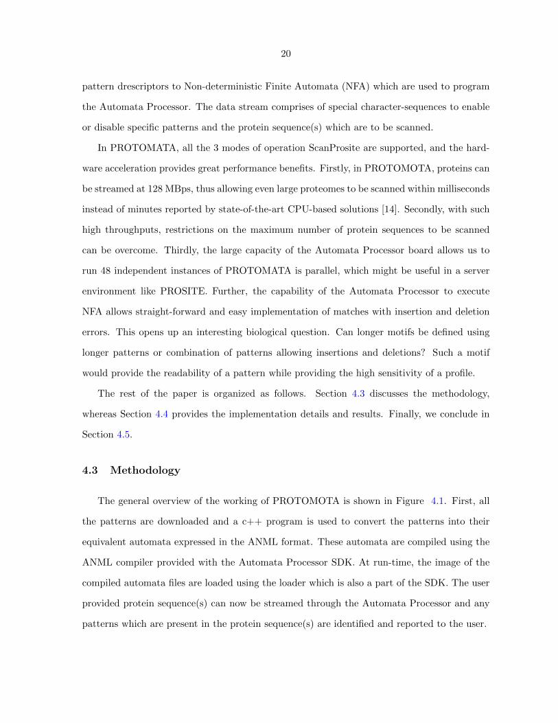
The general overview of the working of PROTOMOTA is shown in Figure 4.1. First, all
the patterns are downloaded and a c++ program is used to convert the patterns into their
equivalent automata expressed in the ANML format. These automata are compiled using the
ANML compiler provided with the Automata Processor SDK. At run-time, the image of the
compiled automata files are loaded using the loader which is also a part of the SDK. The user
provided protein sequence(s) can now be streamed through the Automata Processor and any
patterns which are present in the protein sequence(s) are identified and reported to the user.
21
C++ Executable
Program
Place and Route
Compiler
Prosite PatternFile Converter
Program
ANML to AutomataCompiler
PatternFile
ANMLFile
AutomataFile
OutputMatchedPatternsLoad
Automata file onto
Processor
Active, Programmed
AutomataProcessor
Compile time operations Run-time operations
Protein sequence(s)
Figure 4.1 Overview of the working of PROTOMATA
4.3.1 PROSITE patterns
Prosite patterns are defined as a sequence of pattern elements. Single letter codes as defined
by IUPAC are used to represent amino acids. Prosite allows for the following pattern elements
using the alphabet of amino acids:
• A single amino acid is denoted by a lone amino acid character. For example: S denotes
only the amino acid S.
• One of multiple amino acids is denoted by a series of characters within brackets. For
example: [STG] denotes S or T or G.
• Anything outside of a set of amino acids is denoted by a series of characters within curly
brackets. For example: {STG} denotes any amino acid that is neither S nor T nor G.
• The lower case letter x is used to denote any amino acids.
22
• A pattern can be restricted to the N-terminal of a protein by beginning the pattern with
the character <. For example: < S would only match an S found at the beginning of
the sequence.
• A pattern can be restricted to the C-terminal of a protein by ending the pattern with the
character >. This can also be found in brackets. For example: T > would only match a
T found at the end of the sequence. Similarly [T >] indicates that either a T or the end
of the sequence is acceptable.
• The repetition of a pattern element pe can be defined using parenthesis. This can be
done for a specific number or a range. For example: pe(m) indicates the repetition of pe
m times. Similarly pe(m,n) indicates the repetition of pe anywhere from m to n times
inclusive. Here, m can be zero.
• Each pattern element is separated by a concatenation symbol ’-’. To denote the end of
a pattern the period character ’.’ is used.
An example of a full Prosite pattern is as follows:
PS00008: N-myristoylation site
G− EDRKHPFYW − x(2)− [STAGCN ]− P.
4.3.2 Conversion of PROSITE patterns to ANML automata
For each PROSITE pattern there are 2 automata created: filter-automaton used for iden-
tifying the only those patterns which are present in all the protein sequence(s); and location-
automaton for identifying the location(s) where these sequence(s) where these patterns occur.
This is done to mitigate the amount of output handling and its effect on the run-time of the
entire process. The filter-automaton generates output only at the end of the streaming of all
protein sequence(s) and the location-automaton generates output only at those positions where
a common motif occurs in the sequence(s).
Both the automata are constructed in a modular fashion using macros. The only macro
which changes from one motif to another is the pattern macro. The other macros are used
23
to either enable the search for that motif based on user inputs, or in the case of the filter-
automaton to identify motif common to all the sequences.
A sequential ANML program modeling a pattern can be generated by converting each
item into a set of State Transition Elements (STEs.) Using a conversion executable developed
for this purpose, a unique macro is created for each pattern in an input PROSITE data
file. Each character in a pattern is implemented using a State Transition Element which are
then be connected in the order presented to create the pattern. Single amino acid, one-of-
multiple amino acid, and anything-but amino acid can be directly implementing by shosing
the corresponding character class as the label for the STE. For the wildcard x, an STE with
the character set [A− Z] as the label is used.
For small repetitions and ranges, one STE with a given symbol set is produced for the
maximum number of repetitions. These are linked sequentially and can be considered together
as satisfying the pattern element by linking in to the STE0 and out of STEn where n is the
maximum number of repetitions. In the case of a range pe(m,n), additional links are included
to simultaneously consider all k for m <= k <= n. To achieve this the previous pattern
element in the sequence links to STE0, STE1, STE2...STEn−m.
For large repetitions it begins with a single regular STE. This STE connects to a counter
element which tallies consecutive occurrences. Introduced with the counter is a second STE
with a complemented symbol set to the target. The complimenting STE resets the counter
to zero any time a non-matching amino acid is read. When the counter reaches its target the
counter activates the next pattern element.
For large ranges a system similar to large repetitions is used. For this, the original counter
is used as a lower bound. An additional counter is introduced to act as an upper bound. When
an upper bound is reached both counters are reset.
With all pattern elements represented and connected in ANML the code is collected as
a Pattern Macro. Other supporting macros are used in conjunction with the unique pattern
macros to support more sophisticated functionality. An enable macro is used as a prefix to
each pattern macro. This macro is programmed with a 16b enable code. The beginning of any
24
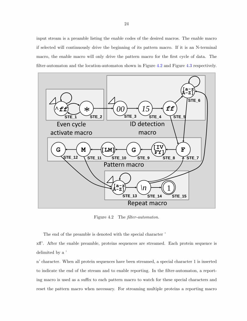
input stream is a preamble listing the enable codes of the desired macros. The enable macro
if selected will continuously drive the beginning of its pattern macro. If it is an N-terminal
macro, the enable macro will only drive the pattern macro for the first cycle of data. The
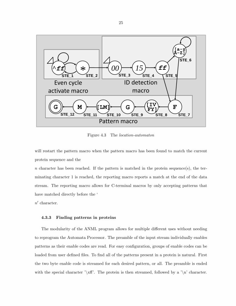
filter-automaton and the location-automaton shown in Figure 4.2 and Figure 4.3 respectively.
^ff * 00 15 ff
[a-zA-Z]
\n 1[a-zA-Z]
FM [LM][IV FY]GG
Even cycle activate macro
ID detection macro
Pattern macro
Repeat macro
STE_1 STE_2 STE_3 STE_4 STE_5
STE_6
STE_7STE_8STE_9STE_10STE_11STE_12
STE_13 STE_14 STE_15
Figure 4.2 The filter-automaton.
The end of the preamble is denoted with the special character ’
xff’. After the enable preamble, proteins sequences are streamed. Each protein sequence is
delimited by a ’
n’ character. When all protein sequences have been streamed, a special character 1 is inserted
to indicate the end of the stream and to enable reporting. In the filter-automaton, a report-
ing macro is used as a suffix to each pattern macro to watch for these special characters and
reset the pattern macro when necessary. For streaming multiple proteins a reporting macro
25
^ff * 00 15 ff
[a-zA-Z]
FM [LM][IV FY]GG
Even cycle activate macro
ID detection macro
Pattern macro
STE_1 STE_2 STE_3 STE_4 STE_5
STE_6
STE_7STE_8STE_9STE_10STE_11STE_12
Figure 4.3 The location-automaton
will restart the pattern macro when the pattern macro has been found to match the current
protein sequence and the
n character has been reached. If the pattern is matched in the protein sequence(s), the ter-
minating character 1 is reached, the reporting macro reports a match at the end of the data
stream. The reporting macro allows for C-terminal macros by only accepting patterns that
have matched directly before the ‘
n′ character.
4.3.3 Finding patterns in proteins
The modularity of the ANML program allows for multiple different uses without needing
to reprogram the Automata Processor. The preamble of the input stream individually enables
patterns as their enable codes are read. For easy configuration, groups of enable codes can be
loaded from user defined files. To find all of the patterns present in a protein is natural. First
the two byte enable code is streamed for each desired pattern, or all. The preamble is ended
with the special character ’\xff’. The protein is then streamed, followed by a ’\n’ character.
26
Finally a 1 is streamed to indicate the end of the file. At the point, all enabled patterns which
were found in the protein report.
This process can be extended to find all patterns present in all of a series of proteins. For
this the enabling mechanism is the same. After this each protein is streamed in order, each
delimited by the ’\n’ character. When an enabled macro has not matched and encounters
a ’\n’ character it is disabled. When the final protein has streamed only patterns that have
matched every protein are enabled and can report.
4.3.4 Finding pattern locations in proteins
After finding the patterns common to all proteins with the common-pattern-finding version
of the program, the locations of these patterns within the proteins must be found. To accom-
plish this, the location-finding version of the program is used. The exact same preamble and
data are streamed. With the location-finding version, reports are generated for each pattern
match for each protein. With this, the matching location for each pattern for each protein of
the motif is known.
4.4 Implementation and results
Prosite defined patterns are available on their website altogether in a single ’.dat’ file. For
this work this file was used, defining 1308 different patterns. A program has been developed to
generically convert patterns defined in this ’.dat’ form to a single ANML program. The ANML
only needs to be generated once and takes 0.87s. The resulting program has 23713 STEs, with
1308 reporting elements or one for each pattern.
This section continues by breaking down the runtime characteristics of the rest of the
process.
4.4.1 Compile-time overhead
Due to the modularity of the designed solution, compiling the ANML code into a placed-
and-routed ’.fsm’ automata file must only be done once. This time is the sum of two com-
27
ponents: 1. The time of compiling the ANML file into an automata file, and 2. The time of
loading the automata file onto the Automata Processor.
Compilation time, automata size and load time vary based on the proteins which are being
represented. This is in the worst case on the order of minutes, and only needs to be performed
once for an indefinite number of instances of the problem. For this reason the compilation and
load times are not considered.
4.4.2 Execution-time overhead
After the programs are in place, the runtime of the application itself must be considered.
This can be divided into three subsections: The preamble, the data streaming, and the read-
out. The time length of the preamble tp can be defined as tp = (2ep + 1) ∗ 7.45 ∗ 10−9 where
ep is the total number of enabled patterns in each version of the program. If all 1308 patterns
were enabled simulatenously for both programs, this yields a maximum combined overhead
cost of 3.899 ∗ 10−5s.
The data streaming must be done completely one time for each of the two versions of the
program. The total time td of this streaming can be defined as td = (7.45 ∗ 10−9) ∗∑n−1
i=0 lpi
where lpi is the length of the ith scanned protein, and n is the total number of scanned proteins.
When scanning 100 proteins of average length 300 this time is 2.235 ∗ 10−4s for each program,
or a combined 4.470 ∗ 10−4s for both.
Finally the read-out time is considered. For the common-pattern-finding version of the
program, all data is reported simultaneously after the terminating character. The readout cost
is a function of the number of patterns in the program. The time tr can be defined as tr =
((d n1000e ∗ 40) + 1) ∗ 7.45 ∗ 10−9s where n is the total number of patterns in the program. For
our 1308 pattern example, this time is 6.035 ∗ 10−7s.
For the location-finding version of the program output is captured as it is generated. Be-
cause each pattern only needs to be matched once to a scanned protein, and because each
scanned protein is of significant length, lp � 40, the readout can be performed in parallel to
the data streaming. The final readout after the data has finished streaming will have proper-
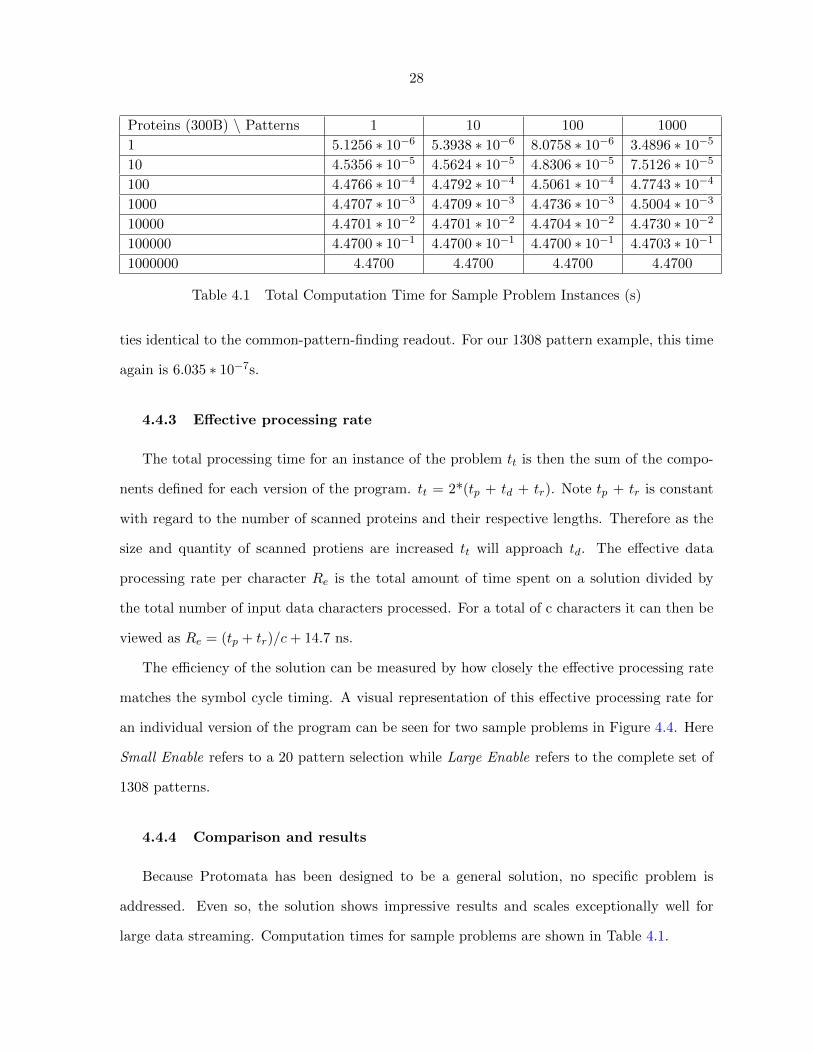
28
Proteins (300B) \ Patterns 1 10 100 1000
1 5.1256 ∗ 10−6 5.3938 ∗ 10−6 8.0758 ∗ 10−6 3.4896 ∗ 10−5
10 4.5356 ∗ 10−5 4.5624 ∗ 10−5 4.8306 ∗ 10−5 7.5126 ∗ 10−5
100 4.4766 ∗ 10−4 4.4792 ∗ 10−4 4.5061 ∗ 10−4 4.7743 ∗ 10−4
1000 4.4707 ∗ 10−3 4.4709 ∗ 10−3 4.4736 ∗ 10−3 4.5004 ∗ 10−3
10000 4.4701 ∗ 10−2 4.4701 ∗ 10−2 4.4704 ∗ 10−2 4.4730 ∗ 10−2
100000 4.4700 ∗ 10−1 4.4700 ∗ 10−1 4.4700 ∗ 10−1 4.4703 ∗ 10−1
1000000 4.4700 4.4700 4.4700 4.4700
Table 4.1 Total Computation Time for Sample Problem Instances (s)
ties identical to the common-pattern-finding readout. For our 1308 pattern example, this time
again is 6.035 ∗ 10−7s.
4.4.3 Effective processing rate
The total processing time for an instance of the problem tt is then the sum of the compo-
nents defined for each version of the program. tt = 2*(tp + td + tr). Note tp + tr is constant
with regard to the number of scanned proteins and their respective lengths. Therefore as the
size and quantity of scanned protiens are increased tt will approach td. The effective data
processing rate per character Re is the total amount of time spent on a solution divided by
the total number of input data characters processed. For a total of c characters it can then be
viewed as Re = (tp + tr)/c + 14.7 ns.
The efficiency of the solution can be measured by how closely the effective processing rate
matches the symbol cycle timing. A visual representation of this effective processing rate for
an individual version of the program can be seen for two sample problems in Figure 4.4. Here
Small Enable refers to a 20 pattern selection while Large Enable refers to the complete set of
1308 patterns.
4.4.4 Comparison and results
Because Protomata has been designed to be a general solution, no specific problem is
addressed. Even so, the solution shows impressive results and scales exceptionally well for
large data streaming. Computation times for sample problems are shown in Table 4.1.

29
Figure 4.4 Protomata Scaling Efficiency
A competing implementation using a Pentium 4, 3.4GHz has been found to map all prosite
patterns on the whole Escherichia coli (E. coli) proteome in about 10 minutes [14]. There
exist 4339 protein sequences in the E. coli proteome, each averaging a length of 287 amino
acids [20]. Given these parameters, the protomata solution is capable of processing the data
in 1.8660 ∗ 10−2s. With additional time allocated for the CPU Protomata can safely boast
an runtime of less than 200ms, resulting in a larger than 3000 times speedup over published
results.
4.5 Conclusion
In this paper, a greatly accelerated solution to scan for PROSITE patterns called PRO-
TOMATA has been presented. In order to provide this acceleration, PROTOMOTA uses a
novel hardware architecture which has been purpose-built to scan thousands of patterns in
parallel. The engine serves to find common defined patterns among proteins as quickly as the
data can be streamed by the Automata Processor, with minimal overhead and only a singularly
30
programmed instance.
Acknowledgment
The authors would like to thank Paul Dlugosch and his team from Micron Technology,
Inc. for providing the Automata Processor boards and sharing valuable insights about how to
program the same.
31
CHAPTER 5 APPLICATION DEVELOPERS’ NOTES
This chapter is dedicated to the discussing the intrinsic details that application developers
should be aware of while designing their automata for the Automata Processor. It also contains
the lessons learnt while programming PROTOMOTA, so that such pitfalls can be avoided in
the future
5.1 Automata Processor Board configuration
The Automata Processor board consists of 48 automata processor cores arranged in 6
ranks of 8 processors each. The Automata Processor cores in a single rank share a high speed
inter-connect which allows them to be presented with the same data flow concurrently. The
processor cores can be logically organized into logical cores and logical core groups to provide
maximum throughput while using the device. A large logical core allows the programmer to
exploit parallelism in terms of the set of automata executing on a single data flow, whereas
the logical core groups allow parallelism through multiple data flows.
A logical core consists of 2, 4 or 8 processor cores from a single rank. All the processor
cores in a logical core are presented with the same data flow. The idea is to allow the execution
of one large automaton or multiple smaller automata which cumulatively take more resources
than what is present on a single core. While designing large automata, one must bear in mind
that the physical routing is limited to only a half-core, which as the name suggests contains half
of the resources present in a single Automata processor core. When the compiler is presented
with an automaton which cannot be fit inside a single half-core, it tries to partition it into
multiple logical parts which can be fit into multiple half-cores inside a single logical core.
When these half-cores are presented with the same data flow, it behaves exactly like the the
32
unpartitioned large automaton. However, one must bear in mind, that the partitioning by the
compiler might not be very efficient, or in the worst case may not be possible at all. On the
other hand, an application developer is cognizant of the design and purpose of the automaton
and may be able to produce a much better logical partitioning of the same. Therefore, the
programmer is well adviced to view a logical core as grouping of half-cores rather than full
Automata Processor cores.
A logical core group consists of 2 or more identically programmed logical cores. These
cores may come from one or more ranks and are presented with different data-flows. The idea
here is to allow the automata logic to be applied to multiple data-flows in parallel for higher
throughput. The logical core groups may be handled by one or more CPU thread(s). In the
case of multiple CPU threads, some of the resources of the Automata Processor board get
distributed amongst the CPU threads. The effects of these partitioning are not clear to the
author at the time of writing this document.
5.2 Finer details for designing automata
Having a basic understanding of the Automata Processor and how to configure it will
allow any user to begin designing solutions. With a deeper understanding of the device and
its configuration, however, users are capable of significantly improving their success in both
development and execution.
5.2.1 Element and routing implementation
Along with the STEs, the Automata Processor also contains counter elements and boolean
elements. The counter elements are used to compress the size of automata, where as the
boolean elements can be used to create automata which have more expressive power than
classical NFA. However, programmers should bear two things in mind: 1) counter and boolean
elements are much less numerous than STEs and 2) the output event from a counter or boolean
element can only be routed to an STE within one cycle.
The counter element is a 12-bit binary down-counter. It is programmed with a value and
33
every time one of the count enable signals is activated, the counter is decremented by 1. When
the count reaches 0, an output event is triggered. The value of a counter can be used but only
at the cost of reading out the entire state vector of the Automata Processor. Counters are very
effective in identifying whether a sub-expression of a regular expression has been matched for
exactly or at least a fixed number of times. Other implementations including those in cellular
automata have also been demonstrated.
The boolean element is a function-programmable combinatorial element which can be can
be programmed to perform the following logical functions: OR, AND, NAND, NOR, sum of
products, and products of sums. The boolean elements can be used for combination of the
results of subexpressions. They can also be programmed with an optional synchronized enable
signal which can be used enable all the boolean elements only when the signal is triggered.
This feature allows for some aspects of dynamic automata computing.
The routing matrix controls the distribution of signals to and from the automata elements,
as programmed by the application. The routing matrix is a complex hierarchical lattice struc-
ture of groups of elements. While in an ideal theoretical model of automata every element
can potentially be connected to every other element, the actual physical implementation in
silicon imposes routing capacity limits related to tradeoffs in clock rate, propagation delay,
die size, and power consumption. All programmable elements are subject to these capacity
limitations placed by the routing matrix. Elements have a maximum in-degree and out-degree
of 16. Automata with larger fan-in or fan-out requirements need duplication of elements. Han-
dling large automata with very high edge densities may create enormous challenges on the
efficient mapping of those automata onto the Automata Processor. This could lead to very
large compilation times as well as low efficiency of the usage of the elements on the Automata
Processor.
5.2.2 Avoiding scaling and routing pitfalls
By definition the Automata Processor reliably allows for the routing of as many as 16
ingoing and 16 outgoing connections for each element of the device. Even if these routing
34
limitations are met, and the number of utilized elements is small enough to fit on a single
half-core, a solution still may not be achievable. Because placing and routing is a difficult
problem, the ANML compiler may struggle with particularly dense and large graphs. Even if
such a compilation is eventually successful, a large compilation time may not be acceptable for
repeatedly configured solutions.
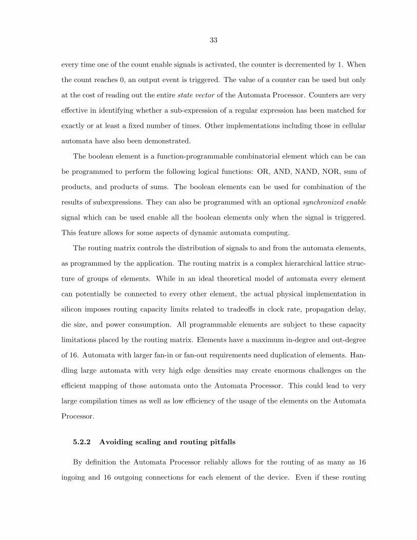
A tree structure is a common example of a difficult to compile graph. A tree structure may
be used for the matching of all possible patterns for a small alphabet. Consider an example
tree used to map genome bases {A,C,G, T} as displayed in Figure 5.1. Although such a tree
may use a conservative number of elements and uses only a fraction of maximum outgoing
connections for each element, compilation may struggle for large depths of the tree.
Figure 5.1 Genome mapping tree solution
Because the routing matrix relies in part on locality, the large fanning of a tree structure can
explode outgoing connection requirements at a region level rather than an individual element
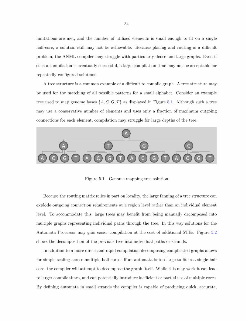
level. To accommodate this, large trees may benefit from being manually decomposed into
multiple graphs representing individual paths through the tree. In this way solutions for the
Automata Processor may gain easier compilation at the cost of additional STEs. Figure 5.2
shows the decomposition of the previous tree into individual paths or strands.
In addition to a more direct and rapid compilation decomposing complicated graphs allows
for simple scaling across multiple half-cores. If an automata is too large to fit in a single half
core, the compiler will attempt to decompose the graph itself. While this may work it can lead
to larger compile times, and can potentially introduce inefficient or partial use of multiple cores.
By defining automata in small strands the compiler is capable of producing quick, accurate,
35
Figure 5.2 Genome mapping decomposed solution
and efficient implementations.
Even in situations where per-element routing is modest, scale must also be considered.
Despite having no directly challenging connection properties, a series of singularly connected
elements in a linked list fashion may cause compilation difficulties if it is several thousand
elements long. Once again, the decomposition of such large and complicated graphs can aid
compilation times at the expense of additional elements. If such difficult automata cannot be
decomposed, considering a different approach to the target problem may be in order.
5.3 Designing robust solutions
While understanding the practical capabilities of the Automata Processor in modeling NFA
is important, a complete solution may extend beyond the definition of a single automata. In
reality a developer must also consider the cost of generating ANML and repeated compilation
for exceptionally large tasks, as well as the managing of input and output data streams. Such
extended considerations may influence the design of the NFA themselves and can be beneficial
in maximizing efficiency across the entire development process.
5.3.1 Multiple automata instances
Often when producing a solution for the Automata Processor, the scale or variability of
the problem requires multiple unique instantiations of a rank or core. It is possible that 1) A
solution requires dynamically produced NFA based on the properties of the problem instance
or 2) A solution requires a set of automata too large to be modeled in one instance of the
36
Automata Processor, or both. In such situations the generation, compilation, and load times
for automata are not simple one-time costs, and must be considered in the total operation time
of a solution. Minimizing these costs can contribute tremendously to the overall performance
of a solution.
5.3.1.1 Managing multiple compilations
Solutions that require unique automata to be developed, compiled, and loaded onto the
Automata Processor for each problem instance should be avoided whenever possible. If a
problem absolutely requires the repeated production of such solutions, ANML generation and
compilation times become targets for overall runtime reduction.
If unique ANML must be written for each problem instance, automation is essential. Al-
though ANML generation applications may bear a large upfront development cost, they are the
only reasonable solution for such repeated code production. While graphical editors may pro-
vide a convenient way to update automata, any such user-dependant modification introduces
delays and potential for error across repeated solutions.
After ANML generation times are addressed, ANML compilation times must be addressed.
Although compilation times can be difficult to predict, they are heavily dependent on the
size and routing of the desired automata. It is strongly advised that if a solution requires
such repeated ANML generation and compilation that the automata are as small and sparsely
connected as possible.
5.3.1.2 Avoiding additional compilation
Although compilation time can be lowered significantly with careful graph design, where
possible it can be best to design solutions that avoid compilation altogether. To avoid defin-
ing unique automata for each instance of a problem, singularly compiled automata can be
implemented using one of two approaches: 1) The automata is designed to have configurable
functionality based on some input metadata or 2) A generic automata can be defined for a
problem where element place and route is consistant for all problem instances.

37
A reconfigurable functionality automata allows for different effective automata implemen-
tations without having to change any connections or values of any elements on the Automata
Processor. Such a solution can be beneficial when a large amount of functionality is prede-
fined and only a subsection of it is relevant for a given problem implementation. Supporting
subgraphs can be added to a solution to enable or disable sections of the main graph based
on metadata. The introduction of such extra streamed input data can reduce the effective
processing rate of an automata, and should be minimized by design. Although metadata may
extend the data stream, reconfigurable solutions will remain significantly faster than recom-
piled solutions.
If instances of a problem require uniquely configured automata that share a common ele-
ment placement and routing, a different approach can be taken. Compiled and loaded automata
can have some or all of their non-routing element properties redefined without compilation.
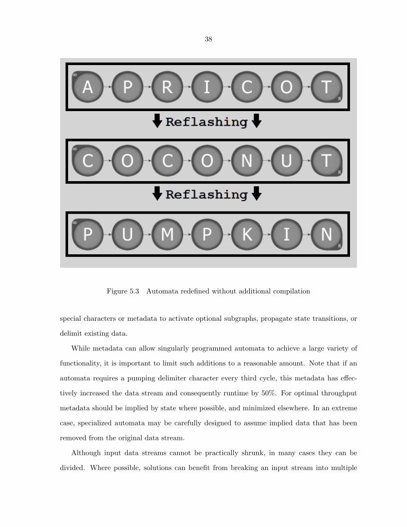
This process is known as reflashing, and is an important strength of the Automata Processor.
While slower than a reconfigurable functionality approach, reflashing is significantly faster than
loading new automata and allows for the disabling of existing sections of the target automata.
An example of basic reflashing can be seen in Figure 5.3. Here, a simple matching automata
is reflashed to find different words of the same size.
5.3.2 Managing input and output data
While input and output data approaches may seem rigid with respect to a given problem,
such properties are often quite flexible and can contribute significantly to the overall perfor-
mance of a solution. Both input data and output reporting introduce unique and important
considerations for the design of a comprehensive solution.
5.3.2.1 Input data streams
For any given problem, a result or partial result is achieved when an automata instance
reaches the end of the input data stream. This data stream in most cases is already in its sim-
plest, most direct form and cannot be reduced. In some cases, automata may require additional
38
Figure 5.3 Automata redefined without additional compilation
special characters or metadata to activate optional subgraphs, propagate state transitions, or
delimit existing data.
While metadata can allow singularly programmed automata to achieve a large variety of
functionality, it is important to limit such additions to a reasonable amount. Note that if an
automata requires a pumping delimiter character every third cycle, this metadata has effec-
tively increased the data stream and consequently runtime by 50%. For optimal throughput
metadata should be implied by state where possible, and minimized elsewhere. In an extreme
case, specialized automata may be carefully designed to assume implied data that has been
removed from the original data stream.
Although input data streams cannot be practically shrunk, in many cases they can be
divided. Where possible, solutions can benefit from breaking an input stream into multiple
39
smaller streams that can be processed in parallel. These processing automata across multiple
cores may be identical or may be specialized for their individual section of the original data
stream. When designing solutions it is important to consider the possibility of such stream
division as the large gains in throughput will often outweigh potential increased resource con-
sumption.
5.3.2.2 Output handling
Output for the Automata Processor is an exceptionally important consideration for the
design of efficient solutions. Each half of an Automata Processor core is divided into three
separate output regions for a total of six across the core. When an STE from a given region
reports a match, it is sent ot the output event memory of that region. From there, each of
the regions output events can be consolidated into the main output event buffer and finally
reported. The process of transferring data from the output event memory to the main output
event buffer costs roughly 40 input symbol cycles. Furthermore, this cost must be paid serially.
If all six output regions report simultaneously, their collective results cannot be reported for
40 ∗ 6 = 240 input symbol cycles.
From this there are two important lessons. First, it is important to consolidate output to
as few regions as possible. Since each region can only support 1024 reporting lines, a solution
may benefit from having fewer or more selective reporting cases. It can be advantageous to
have multiple reporting elements with the same goal feed into a smaller representative set of
reporting elements.
Secondly, it is important to minimize the amount of reporting in general. Where possible
it can be advantageous to have multiple elements wait to report simultaneously or at the end
of data. Solutions that require constant small reports of data with only a small number of
cycles between each event will perform poorly. A cohesive solution must recognize that the
CPU must still handle all of the data that is returned by the Automata Processor. A naive
or greedy solution may even produce more data than it takes in, and such solutions should be
considered with extreme caution.
40
CHAPTER 6 CONCLUSION
The Automata Processor is shown to be an extremely promising new processing architecture
for large scale pattern matching applications. In the field of Bioinformatics, search for motif
patterns in protein sequences provides one such application. PROSITE is a large annotated
database of known protein motifs and currently contains 1308 known protein motifs expressed
as patterns. Due to the large capacity of the Automata Processor, the automata for all these
motif-patterns can be loaded and executed in the Automata Processor in parallel. This gives
rise to large scale speed-up with respect to execution times of existing software. For example,
all proteins present in the proteome of Escherichia coli (E.coli) can be scanned against all
motif-patterns in less than 100 milliseconds. This is more than a 6000 times speed-up over
published execution times. Furthermore, when the automata for all these motif-patterns are
loaded onto the Automata Processor chip, they collectively take up about half of the resources
of the chip. Since a single rank contains 8 Automata Processor chips and the automata for
all motif-patterns which can fit into a single rank can be executed in parallel, the execution
time for any given protein sequence will remain constant for a motif-database which is up to
16 times of the current size.
Though PROTOMOTA currently provides a command-line interface only, it supports all
the modes of operation provided by the PROSITE website, and more. In the first mode
of operation, PROTOMOTA supports the scanning for all known motifs in a given protein
sequence; or all common motifs in multiple protein sequences. Here PROTOMOTA not only
provides a more fine-grained control over motifs being searched for, but also does not place an
upper limit of 8 on the number of protein sequences as in the case of the PROSITE website. In
the second mode of operation the presence of a particular motif can be detected in all proteins
41
in the database.
PROTOMATA was designed not only to aid biologists in the characterization of a vastly
growing number of newly sequenced proteins, but also to serve as a guide for application
developers in the field to develop programs on this new accelerator architecture. Therefore,
the automaton for any motif is defined in a modular and easy to understand manner using
the macros. The script to generate the automaton from a motif-pattern is also provided. This
also makes it easy to handle new motifs which will be added to the PROSITE database or are
under the investigation of a user.
Future work in this direction consists of executing this software on the real Automata
Processor board and making the same available to everybody through a web-based interface.
This interface may complement or be part of the PROSITE website. Further, the lessons
learnt while developing the PROTOMOTA application (and mentioned in the application
developers notes) would play a more significant role while developing larger and more complex
bioinformatics problems in the future.
In general, more and more applications in various fields are being successfully designed
and implemented on the Automata Processor. The processor has already been shown to
considerably accelerate applications in the field of network security, image processing and
machine learning, etc. Future generations of the processor which place lower restrictions on
the resource requirements of the automata design are already in the works. Though thinking
in terms of NFA can be difficult at first, but it paves the way for more natural exploration of
difficult problems. The advent of the Automata Processor will provide a way to execute these
NFA directly on the processor. With its large capacity to execute thousands of automata in
parallel, it will a promising architecture for which to watch out.
42
Bibliography
[1] Perl compatible regular expressions.
[2] Janusz Brzozowski and Hellis Tamm. Theory of atomata. In Developments in Language
Theory, pages 105–116. Springer, 2011.
[3] Cezar Campeanu, Nicolae Santean, and Sheng Yu. Mergible states in large nfa. Theoretical
computer science, 330(1):23–34, 2005.
[4] Chang Chia-Hsiang and Robert Paige. From regular expressions to dfa’s using compressed
nfa’s. Theoretical Computer Science, 178(1):1–36, 1997.
[5] Edouard De Castro, Christian JA Sigrist, Alexandre Gattiker, Virginie Bulliard, Petra S
Langendijk-Genevaux, Elisabeth Gasteiger, Amos Bairoch, and Nicolas Hulo. Scanprosite:
detection of prosite signature matches and prorule-associated functional and structural
residues in proteins. Nucleic acids research, 34(suppl 2):W362–W365, 2006.
[6] Philippe Dessen, Christian Fondrat, Claire Valencien, and Claude Mugnier. Bisance: a
french service for access to biomolecular sequence databases. Computer applications in
the biosciences, 6(4):355–356, 1990.
[7] Paul Dlugosch, Dave Brown, Paul Glendenning, Michael Leventhal, and Harold Noyes.
An efficient and scalable semiconductor architecture for parallel automata processing.
Transactions on Parallel and Distributed Systems, 2013.
[8] Paul Dlugosch, Dave Brown, Paul Glendenning, Michael Leventhal, and Harold Noyes. An
efficient and scalable semiconductor architecture for parallel automata processing. IEEE
Transactions on Parallel and Distributed Systems, 2013, in press.
43
[9] Rainer Fuchs. Macpattern: protein pattern searching on the apple macintosh. Computer
applications in the biosciences: CABIOS, 7(1):105–106, 1991.
[10] Rainer Fuchs. Predicting protein function: a versatile tool for the apple macintosh. Com-
puter applications in the biosciences: CABIOS, 10(2):171–178, 1994.
[11] Christophe Geourjon and Gilbert Deleage. Interactive and graphic coupling between multi-
ple alignments, secondary structure predictions and motif/pattern scanning into proteins.
Computer applications in the biosciences: CABIOS, 9(1):87–91, 1993.
[12] Steven Henikoff and Jorja G Henikoff. Automated assembly of protein blocks for database
searching. Nucleic Acids Research, 19(23):6565–6572, 1991.
[13] Jan Holub. Dynamic programmingnfa simulation. In Implementation and Application of
Automata, pages 295–300. Springer, 2003.
[14] Nicolas Hulo, Amos Bairoch, Virginie Bulliard, Lorenzo Cerutti, Beatrice A Cuche,
Edouard De Castro, Corinne Lachaize, Petra S Langendijk-Genevaux, and Christian JA
Sigrist. The 20 years of prosite. Nucleic acids research, 36(suppl 1):D245–D249, 2008.
[15] LF Kolakowski Jr, JA Leunissen, and JE Smith. Prosearch: fast searching of protein
sequences with regular expression patterns related to protein structure and function.
Biotechniques, 13(6):919–921, 1992.
[16] Peter R Sibbald and Patrick Argos. Scrutineer: a computer program that flexibly seeks
and describes motifs and profiles in protein sequence databases. Computer applications
in the biosciences: CABIOS, 6(3):279–288, 1990.
[17] Christian JA Sigrist, Edouard De Castro, Lorenzo Cerutti, Beatrice A Cuche, Nicolas
Hulo, Alan Bridge, Lydie Bougueleret, and Ioannis Xenarios. New and continuing devel-
opments at PROSITE. Nucleic acids research, 41(D1):D344–D347, 2013.
[18] Rodger Staden. Screening protein and nucleic acid sequences against libraries of patterns.
Mitochondrial DNA, 1(6):369–374, 1991.

44
[19] Michael JE Sternberg. Promot: a fortran program to scan protein sequences against a
library of known motifs. Computer applications in the biosciences: CABIOS, 7(2):257–
260, 1991.
[20] Axel Tiessen, Paulino Perez-Rodrıguez, and Luis J Delaye-Arredondo. Mathematical
modeling and comparison of protein size distribution in different plant, animal, fungal and
microbial species reveals a negative correlation between protein size and protein number,
thus providing insight into the evolution of proteomes. BMC research notes, 5(1):85, 2012.
[21] Kuo-Kun Tseng, Yuan-Cheng Lai, Ying-Dar Lin, and Tsern-Huei Lee. A fast scalable
automaton-matching accelerator for embedded content processors. ACM Transactions on
Embedded Computing Systems (TECS), 8(3):19, 2009.
[22] James C Wallace and Steven Henikoff. Patmat: a searching and extraction program
for sequence, pattern and block queries and databases. Computer applications in the
biosciences: CABIOS, 8(3):249–254, 1992.
[23] Hao Wang, Shi Pu, Gabe Knezek, and J Liu. Min-max: A counter-based algorithm for
regular expression matching. 2013.
[24] Yi-Hua Yang and Viktor K Prasanna. High-performance and compact architecture for
regular expression matching on fpga. Computers, IEEE Transactions on, 61(7):1013–1025,
2012.
[25] Yuan Zu, Ming Yang, Zhonghu Xu, Lin Wang, Xin Tian, Kunyang Peng, and Qunfeng
Dong. Gpu-based nfa implementation for memory efficient high speed regular expression
matching. ACM SIGPLAN Notices, 47(8):129–140, 2012.