advisor: olsted jakob g. r - projekter.aau.dk · dernæst beskrives teori om lineære mixed...
TRANSCRIPT

AALBORG UNIVERSITY
REPREATED MEASUREMENTS
THE EFFECT OF IBUPROFEN ON WRIST FUNCTIONS AFTER COLLESFRACTURE
Author:Lotte WOLSTED
Advisor:Jakob G. RASMUSSEN
May 31st 2018

Copyright © Aalborg University 2018Front page is illustrated by Casper Vagnø Wolsted

i
School of Engineering and ScienceInstitut for Matematiske Fag
Skjernvej 4ADK-9220 Aalborg Ø
http://www.math.aau.dk
Title: Repeated measurements
Subject: The effect of Ibuprofen on wrist functions after Colles fracture
Author: Lotte Wolsted
Advisor: Jakob G. Rasmussen
Copies: 2
Pages: 104
Project periode: Spring semester 2018
Handin date: May 31st 2018
Synopsis:The purpose of this report is to determine whether Ibuprofen has any beneficial effect, wrt. recoveryof wrist functions, on patients having been through surgery to correct a Colles fracture. The patientshave been treated with either Ibuprofen or a placebo drug. At three timepoints after the surgery,measurements of how far the patients are able to bend and rotate their injured wrist have beenrecorded. If Ibuprofen does have a beneficial effect, we should be able to see, that the patients, whowere given Ibuprofen, faster regain full mobility of the injured wrist than the patients, who were givena placebo drug.
To determine whether there is a difference between treatment groups, I will use three approaches.First, I will use ANOVA and multivariate ANOVA. This approach is a little too simple to say anythingfinal about the relationship between the treatment groups, but it does give some idea of whetherthere might be a difference in the groups. Next, I will use linear mixed effects models (LMMs). Thetreatment may have an effect on the measurements, but how well the patients are able to bend androtate their wrist may also be influenced by themselves, by some genetic effect. Without having toactually specify any genetic markers, the LMM takes these individual effects into account by allowingfor random effects in the setup of the model. With the LMM, it is also possible to account for anykind of correlation between observations on the same subject. In order to use the LMM, a handful ofassumptions about the model needs to be satisfied. Lastly, I will use generalized estimating equationsmodels (GEE-models). This approach resembles the LMM and it also allows for specification ofcorrelation between observations on the same subject. An advantage of the GEE-model is that thereare no model assumptions to be met. A disadvantage is, that it is not possible to specify random effects.
The results from both ANOVA, multivariate ANOVA, the LMMs and the GEE-models are all unanimous;there is no difference in the treatment groups, i.e. Ibuprofen has no significant beneficial effect.
mellemrumThe content of this report is freely available, but publication (with reference) may only be pursued due to agreement with the
author.

ii
Referat
I denne rapport undersøges det om indtagelse af Ibuprofen forbedrer helningsprocessen for patienteropereret for Colles fraktur. Med helningsproces menes der, hvor hurtigt de genvinder mobilitet af denskadede hånd. Patienterne er inddelt i tre grupper ift. den medicin, de har taget i ugen efter operationen.På tre tidspunkter i løbet af det første år efter operationen, er der målt i grader, hvor meget patienternekan bøje og rotere den skadede hånd. Samme målinger er lavet på den ikke-skadede hånd for at have etmål for, hvor meget hænderne normalt bør kunne bøjes og roteres.
For at undersøge om der er forskel i målingerne på de tre patientgrupper, udføres først både en ANOVAtest og en multivariat ANOVA test. Disse test er blot med for at give en indikation af, om der er forskel pågrupperne.
Dernæst beskrives teori om lineære mixed modeller. Det er muligt, at raten for patienternes helningspro-ces er påvirket af deres gener. Det anvendte datasæt indeholder ingen genetiske variable, så det er ikkemuligt at opstille en almindelige lineær model, hvori der indgår variable for diverse gener for på denmåde at tage højde for evt. genetisk indflydelse. Vha. den lineære mixed model kan vi dog tage højdefor, at helningsprocessen kan være påvirket af ikke-målte faktorer via random effects. Vi er nødt til at tagehøjde for, at målingerne hen over tiden for hver patient kan være korrelerede på en eller anden måde.Dermed er det nødvendigt at anvende en model, der kan indkorporere diverse former for korrelationmellem målingerne. I den almindelige lineære model antages samtlige målinger at være uafhængige.Den lineære mixed model tillader en række af forskellige korrelationsstrukturer.
Slutteligt beskrives teori om generaliserede estimationsligninger (GEE-modeller). Denne tilgang minderlidt om lineære mixed modeller i den forstand, at de er anvendelige i tilfælde med korreleret GLM-agtigtdata. Fordelen ved GEE-modeller er, at man ikke behøver gøre sig antagelser om fordelingen af hverkendata eller fejlledene, hvilket er nødvendigt, hvis man anvender lineære mixed modeller. En ulempe erdog, at man ikke kan specificere random effects. Vha. random effects kan man komme helt ned ogsige noget om de patient-specifikke effekts. I GEE-modeller kan vi "kun” undersøge den gennemsnitligeeffekt i grupperne. Da vi ikke er interesserede i at følge hver enkelt patient for at finde den bedste be-handling for ham/hende, men istedet gerne vil vide om den allerede anvendte behandling generelt harmedført en forskel i helningsprocesserne blandt grupperne, så giver det ganske god mening at anvendeen GEE-model.
Resultaterne fra både ANOVA, multivariat ANOVA, den lineære mixed model og GEE-modellen peger allepå, at der ingen forskel er på patientgrupperne. Dermed har indtagelse af Ibuprofen ingen signifikantindflydelse på helningsprocessen.mellemrummellemrummellemrummellemrummellemrummellemrummellemrummellemrummellemrummellemrum

iii
mellemrummellemrummellemrummellemrummellemrummellemrum

Contents
Preface 1
Notation and other helpful information 1
Acknowledgements 2
1 Description of data 3
2 Analysis of variance 72.1 ANOVA . . . . . . . . . . . . . . . . . . . . . . . . . . . . . . . . . . . . . . . . . . . . . . . . . . 7
2.1.1 Sphericity . . . . . . . . . . . . . . . . . . . . . . . . . . . . . . . . . . . . . . . . . . . . 82.2 MANOVA . . . . . . . . . . . . . . . . . . . . . . . . . . . . . . . . . . . . . . . . . . . . . . . . . 92.3 The ANOVA model . . . . . . . . . . . . . . . . . . . . . . . . . . . . . . . . . . . . . . . . . . . 11
3 Results of using ANOVA and MANOVA on the data 133.1 Testing assumptions . . . . . . . . . . . . . . . . . . . . . . . . . . . . . . . . . . . . . . . . . . 133.2 Analysis using aov() . . . . . . . . . . . . . . . . . . . . . . . . . . . . . . . . . . . . . . . . . . 153.3 Analysis using manova() . . . . . . . . . . . . . . . . . . . . . . . . . . . . . . . . . . . . . . . . 163.4 Conclusion . . . . . . . . . . . . . . . . . . . . . . . . . . . . . . . . . . . . . . . . . . . . . . . . 163.5 Source code: superANOVA() . . . . . . . . . . . . . . . . . . . . . . . . . . . . . . . . . . . . . 16
4 Mixed models 194.1 Setting up the mixed model . . . . . . . . . . . . . . . . . . . . . . . . . . . . . . . . . . . . . . 20
4.1.1 The linear mixed effects model . . . . . . . . . . . . . . . . . . . . . . . . . . . . . . . . 224.2 Estimation and prediction of effects . . . . . . . . . . . . . . . . . . . . . . . . . . . . . . . . . 23
4.2.1 Known covariance . . . . . . . . . . . . . . . . . . . . . . . . . . . . . . . . . . . . . . . 234.2.2 Unknown covariance . . . . . . . . . . . . . . . . . . . . . . . . . . . . . . . . . . . . . . 24
4.3 Covariance structure . . . . . . . . . . . . . . . . . . . . . . . . . . . . . . . . . . . . . . . . . . 264.3.1 Expressing ui using autoregressive structure . . . . . . . . . . . . . . . . . . . . . . . . 274.3.2 Estimating σ2, σ2
u and ρ . . . . . . . . . . . . . . . . . . . . . . . . . . . . . . . . . . . . 284.4 Kenward-Roger approximation . . . . . . . . . . . . . . . . . . . . . . . . . . . . . . . . . . . . 304.5 Fitted values of the LMM . . . . . . . . . . . . . . . . . . . . . . . . . . . . . . . . . . . . . . . . 314.6 The LMM with random intercepts and slopes . . . . . . . . . . . . . . . . . . . . . . . . . . . 35
5 Results of modelling data with LMMs 375.1 Analysis using correlation = corCAR1() . . . . . . . . . . . . . . . . . . . . . . . . . . . . 375.2 Analysis using correlation = corSymm() . . . . . . . . . . . . . . . . . . . . . . . . . . . . 485.3 Analysis using correlation = NULL . . . . . . . . . . . . . . . . . . . . . . . . . . . . . . . . 505.4 Comparison of the "ar”-, "un”- and the "in”-models . . . . . . . . . . . . . . . . . . . . . . . 505.5 Conclusion . . . . . . . . . . . . . . . . . . . . . . . . . . . . . . . . . . . . . . . . . . . . . . . . 535.6 Source code: superLMM() . . . . . . . . . . . . . . . . . . . . . . . . . . . . . . . . . . . . . . . 53
6 Generalized Estimating Equations 556.1 Generalized linear models . . . . . . . . . . . . . . . . . . . . . . . . . . . . . . . . . . . . . . . 556.2 GEE models . . . . . . . . . . . . . . . . . . . . . . . . . . . . . . . . . . . . . . . . . . . . . . . 59
6.2.1 GEE estimation of parameters . . . . . . . . . . . . . . . . . . . . . . . . . . . . . . . . 596.3 GEE vs. LMM . . . . . . . . . . . . . . . . . . . . . . . . . . . . . . . . . . . . . . . . . . . . . . 65

CONTENTS v
7 Results of modelling data with GEEs 677.1 Analysis using corstr = "ar1" . . . . . . . . . . . . . . . . . . . . . . . . . . . . . . . . . . . 687.2 Analysis using corstr = "unstructured" . . . . . . . . . . . . . . . . . . . . . . . . . . . . 717.3 Analysis using corstr = "independence" . . . . . . . . . . . . . . . . . . . . . . . . . . . . 727.4 Comparison of the "ar”-, "un”- and the "in”-models . . . . . . . . . . . . . . . . . . . . . . . 727.5 Conclusion . . . . . . . . . . . . . . . . . . . . . . . . . . . . . . . . . . . . . . . . . . . . . . . . 737.6 Source code: superGEE() . . . . . . . . . . . . . . . . . . . . . . . . . . . . . . . . . . . . . . . 73
8 A different setup 758.1 Clustered LMMs . . . . . . . . . . . . . . . . . . . . . . . . . . . . . . . . . . . . . . . . . . . . . 758.2 Clustered GEE models . . . . . . . . . . . . . . . . . . . . . . . . . . . . . . . . . . . . . . . . . 788.3 Conclusion . . . . . . . . . . . . . . . . . . . . . . . . . . . . . . . . . . . . . . . . . . . . . . . . 80
9 Discussion 81
Appendix A 83
Appendix B 97
Literature 103

Preface
I have been given a data set with patients all of whom had suffered a Colles fracture. All received thesame type of corrective surgery and, subsequently, were placed in one of three groups according totreatment. Some were given Ibuprofen for the pain while others were treated with a placebo drug. Theobjective is to find out whether there is a difference between the patients treated with Ibuprofen and thepatients treated with a placebo drug wrt. how well and how fast they regain mobility of the injured handin the course of a year after surgery. If the type of treatment plays no role in the patients’ recovery, thenthe costs of treatment can be reduced as no pain medicin needs to be prescribed. It is suspected thatIbuprofen may cause bone deterioration, which is another reason to want to find out whether patientsdo just as well without the drug wrt. recovery of wrist functions. The hypotheses to be tested are
• H main0 : There is no difference wrt. recovery of wrist functions between the treatment groups.
• H mainA : Patients treated with Ibuprofen have a better rate of recovery than the other patients.
I will be working with a lot of hypotheses during the report. To distinguish these, I am adding appropri-ate superscripts. I should also note, that when I say a hypothesis is true, what I really mean is, that thereis no evidence to reject it. Three different types of movement of the injured hand have been recorded.This means that each patients’ response is multivariate. Furthermore, these recordings were made atthree different timepoints after the surgery. This means that we have not just one response per patientper type of movement, but instead have a vector of responses for each patient, i.e. we have repeatedmeasurements. While the responses between patients certainly are independent, the entries within eachvector of responses may very well be correlated. An ordinary linear model or a generalized linear modelcannot handle responses being correlated, and as such a different approach is needed. One approach isto use analysis of variance in which the means of each group of patients are compared. This approach,however, does not allow for comparison across timepoints. Another approach is the mixed model, whichis essentially just a linear model with random effects added into the linear predictors. The idea is thatthe dependence between observations within and between groups are effected by some latent variables.The mixed model allows for a wide range of correlation patterns. A third approach is to use quasi like-lihood and generalized estimating equations. When using quasi likelihood, no assumptions about thedistribution of the observations are needed; specifying the mean and variance is all that is required. Inorder to estimate the unknown parameters, the generalized estimating equations are used, in which thecorrelation structure of the observations is specified. I will use all three approaches.
The theory behind each of the three approaches are described in seperate chapters. Each of these chap-ters are followed by a chapter in which the data is analysed in R using the theory just described. Each ofthese chapters end with a conclusion as to whether H main
0 is rejected or not based on the analysis.
Notation and other helpful information
All calculations and figures are made in the statistical software program R. References to R-code will bewritten in a certain font such as geeglm().
To save myself a lot of repeated coding, I have made three functions that do just about everything Ineed in my analysis with the three approaches. These functions are called superANOVA(), superLMM()and superGEE(). Depending on which of the three approaches, I am working with, these functions doanything from testing model assumptions to plotting residuals and calculating standard errors. The in-

2
terested reader can find the source code for these functions in the chapters, where they are used.
References to various literature are noted in brackets [ ], e.g. [9].
For a smoother read, some of the theoretical calculations and results are omitted from the pages, wherethey are used. These calculations/results will be listed in Appendix A. All references to the appendix willbe denoted by e.g. A.3; this is a reference to the 3rd result in Appendix A. Appendix B contains additionaltheory. The reader may use this to acquaint or re-acquaint themselves with some of the theory other-wise left out of the chapters. References to Appendix B is denoted by e.g. B.3.
All vectors or matrices are noted in bold letters. Vectors are always in small letters, and matrices arealways in capital letters. Random variables are noted in non-bold capital letters. Random vectors arenoted in bold capital letters, like matrices. It should be clear from context which is which. If nothingelse is specified, all vectors will be column vectors, i.e.
x =
x1...
xn
= [x1, . . . , xn
] ∈Rn×1.
A row vector will be denoted as a transposed column vector, e.g. xT = [x1 . . . xn
] ∈R1×n .
Let In×n = I ∈Rn×n denote the identity matrix, and let 1n = [1, . . . ,1] ∈Rn×1 denote a vector of all 1s.
At times during calculations in the report, I will refer to other equations in the calculations themselves.These references will be noted above =, ≤, ∝ and the likes. For example
ab(4.1)= c.
Here, I am using equation 1 from Chapter 4 in order to show than ab can be written as c.
A diagonal matrix is noted by
A =
a1. . .
an
= diag{ai }i=1,...,n .
An entry in a matrix may be denoted by A j ,k . This is the element in the j th row and kth column in A.
The determinant of a matrix is noted by |A|.
All examples ends with a square, ä.
At times, I will digress from whatever theory is being described to make a comment about my data. Toavoid having to write "Wrt. my data...” too many times, I use a "!” to stress that I am making a commentabout my data.
Acknowledgements
I would like to thank my advisor, Jakob G. Rasmussen, for constructive critisisme and ideas during thecourse of this project. I would also like to thank Marius Aliuskevicius, M. D. at Aalborg University Hos-pital, for lending me the data for analysis.

1 | Description of data
The data consists of 83 patients, whom have all suffered a Colles fracture (broken bone in the wrist). Allhave received the same surgery from the same surgeon. They have all been treated by the same medicalteam, and all data on the patients have been recorded by the same people. In other words, all patientshave received the same kind of treatment all through the experiment, apart from the type of drug theyhave been treated with. The patients were randomized into three groups and had to take medicine thefirst seven days after surgery. Group 1 took a placebo drug, group 2 took Ibuprofen for three days anda placebo drug for the next four days and group 3 took Ibuprofen. There are 28 patients in group 1and group 2, and 27 patients in group 3. Three pairs of movement of the wrist were recorded on eachpatient at 6 weeks, 3 months and one year after the surgery. The movements are pronation and supina-tion (rotating hand), extension and flexion (bending hand forward and backward) and ulnar and radial("waving” hand from side to side). The same movements have been recorded on the uninjured hand,though only once.
I received three datasets; one with the measurements in degrees of the uninjured hand, one with themeasurements in degrees of the injured hand, and one that describes in percentages how close theranges of movement of the injured hand is to the ranges of the uninjured hand. By "range”, I meanthe degrees from, for instance, the hand bending as far forward as possible to the hand bending as farbackward as possible. I will be working only with the dataset with measurements given in percentages.I have gathered all these measurements in a new dataset, I call Wrist. Below are the first nine rows ofWrist:
1 > head ( Wrist , 9 )2 subject ps ef ur time group3 1 id01 72.22222 36.000000 40.00000 0 14 2 id01 86.11111 68.000000 80.00000 7 15 3 id01 94.44444 68.000000 50.00000 46 16 4 id02 91.17647 47.058824 37.50000 0 17 5 id02 91.17647 76.470588 62.50000 7 18 6 id02 97.05882 76.470588 100.00000 46 19 7 id03 68.57143 4.166667 22.22222 0 1
10 8 id03 94.28571 79.166667 77.77778 7 111 9 id03 97.14286 91.666667 100.00000 46 1
The first column, subject, contains an id identifying each patient. The second column, ps, are all themeasurements for the ranges in percentages of pronation and supination, which I will henceforth justcall the pro/sup-movement. There are three measurements of the pro/sup-movement for each patient;one taken at 6 weeks after surgery (1st timepoint), one taken 3 months after surgery (2nd timepoint)and one taken one year after surgery (3rd timepoint), and they are listed in that order. The same goesfor the ex/flex- and uln/rad-movements (the columns ef and ur). The fifth column, time, indicate atwhat timepoint the measurement was taken. In order to indicate that the time between timepoints isnot equidistant, I have decided not to code the timepoints as "1”, "2”, "3”, which would have been anobvious way of coding the timepoints. Instead, I have coded the timepoints so they show how many(approximately) weeks have passed since the first timepoint. For the 2nd timepoint, approximately 7

1 Description of data 4
weeks have passed. This is calculated by estimating how many weeks are in three months:
52 weeks in a year
12 months in a year≈ 4.333 weeks per month
⇓4.333 ·3 = 13 weeks in three months.
Then the initial 6 weeks until the 1st timepoint must be subtracted, which gives 7 weeks between the1st and 2nd timepoint. Between the 1st and 3rd timepoint, 46 weeks have passed, which is calculatedsimply by 52−6 = 46 weeks. The last column, group, indicate which of the three treatment groups, thepatient belongs to, either "1”, "2” or "3”.
Just to get an initial idea of whether there might be a difference in the responses from the treatmentgroups, I have made Figure 1. This figure shows for each type of movement, how well in percentagesthe injured hand on average per group performs in comparison to the uninjured hand on average pergroup. There are no obvious differences between the groups. Only in the first plot do group 3 seem todo a little better.
●
●
●
6070
8090
ps
Per
cent
age
of n
orm
al r
ange
6 weeks 3 months 1 year
●
●
●
6070
8090
6 weeks 3 months 1 year
●
●
●
6070
8090
6 weeks 3 months 1 year
gr. 1gr. 2gr. 3 ●
●
●
2030
4050
6070
8090
ef
Time after surgery
6 weeks 3 months 1 year
●
●
●
2030
4050
6070
8090
6 weeks 3 months 1 year
●
●
●
2030
4050
6070
8090
6 weeks 3 months 1 year
gr. 1gr. 2gr. 3 ●
●
●
3040
5060
7080
90
ur
6 weeks 3 months 1 year
●
●
●
3040
5060
7080
90
6 weeks 3 months 1 year
●
●
●
3040
5060
7080
90
6 weeks 3 months 1 year
gr. 1gr. 2gr. 3
Figure 1: Each line represent the average percentage of normal range of the pro/sup-, ex/flex- and uln/rad-movements for each group.
Figure 2 show boxplots of the ranges of movement at the different timepoints. If H main0 is true, we might
expect to see, that the median for group 3 is larger than for the other two groups. This is actually the casein the majority of the boxplots, but the differences in the medians are only very small.

1 Description of data 5
●
●
1 2 3
2040
6080
ps.week
●
●●
1 2 3
6070
8090
ps.month
●
●
●
1 2 3
6070
8090
ps.year
1 2 3
020
4060
80
ef.week
Per
cent
age
of n
orm
al r
ange
●
1 2 3
4060
8010
0
ef.month
●
●
●
●
●
●
●
1 2 3
4060
8012
0
ef.year
●
1 2 3
1030
5070
ur.week
●
1 2 3
4060
8012
0 ur.month
Groups
●
●
●
●
●
1 2 3
6010
014
0
ur.year
Figure 2: Boxplots of the percentage of normal range of the movements at different timepoints.
A quick and very simple way of getting an idea of the results, we may encounter later on, is to set upa linear model for each type of movement and compare it to an equivalent linear model without thegroup-term. For comparison, I use anova()1, which tests the hypothesis2
H anova0 : the models are not significantly different.
The relationship between the types of movement and the covariates, group and time, is not linear, but,having investigated this further, linearity can in this case be achieved by adding a squared term of thetimepoints to the models. Below are the results from comparing each of the linear models with theirreduced counterparts:
1 > anova (lm( ps ~ time + I ( time^2) , data = Wrist ) ,2 + lm( ps ~ group + time + I ( time^2) , data = Wrist ) ) $"Pr( >F) " [ 2 ]3 [ 1 ] 0.0643145 > anova (lm( ur ~ time + I ( time^2) , data = Wrist ) ,6 + lm( ur ~ group + time + I ( time^2) , data = Wrist ) ) $"Pr( >F) " [ 2 ]7 [ 1 ] 0.576258
1See B.1.2H anova
0 is equavalent to H anova10 in B.1.

1 Description of data 6
9 > anova (lm( ef ~ time + I ( time^2) , data = Wrist ) ,10 + lm( ef ~ group + time + I ( time^2) , data = Wrist ) ) $"Pr( >F) " [ 2 ]11 [ 1 ] 0.05631
With a significance level of 0.05, each of these p-values indicate that the group-term is insignificant tothe models, although for the pro/sup- and ex/flex-movement, we are not far from rejecting H anova
0 . Thelinear model is a little too simple to model the types of movement properly, but it does give some ideaof the relevance of the treatment groups.
To get a clearer indication of whether there might be a difference between the groups, I will now moveon to my first idea of testing H main
0 . In Chapter 2, the theory behind analysis of variance is explained andin Chapter 3, I test to see if H main
0 should be rejected when using analysis of variance.

2 | Analysis of variance
In order to determine whether there is a difference in the responses from a study where subjects areseperated into groups, one can perform a test to compare the group means. Analysis of variance (ANOVAfor short) is a method for multiple comparisons, meaning two or more groups can be compared. InANOVA, the variation within the samples and the variation between the samples are used to detect dif-ferences in the means. In a one-way ANOVA, the objective is to compare means of two or more samples,where groups are formed according to levels in one factor (hence one-way ANOVA).
The ANOVA is also known as the univariate ANOVA, as it assumes a univariate response. An exten-sion of the univariate ANOVA is the multivariate ANOVA (MANOVA), which assumes a multivariate re-sponse. Both ANOVA and MANOVA are methods for comparing group means, however, neither ANOVAnor MANOVA allows us to compare group means across timepoints.
! It may seem, as I have a multivariate response for each patient in my data, that only MANOVAis of interest, but I shall use both ANOVA and MANOVA to cement my conclusion about whethertreatment plays a significant role in the patients’ recovery. With ANOVA, I will just have to test eachtype of movement seperately.
A group can be several things. If a study consisted of recording some patients’ blood pressure, say, oncea month for a year, then each patient can be thought of as forming a group (or sample). In this case, theresponse for each patient is a vector. A study could also consist of the scores from some test distributedto, say, 7th graders. In this case, we only have one response per subject in the study. A possible choicefor groups could be boys and girls. An observation, yi j , can then either be an observation on the i thsubject at the j th timepoint, or an observation on the j th subject in the i th group. In the following, yi j
is thought of as the observation on subject j in the i th group, but it need not be.
2.1 ANOVA
This section is based on [1] and [2].
In the univariate case, we have g independent samples (or groups)
y1 =[
y11, y12, . . . , y1n1
]y2 =
[y21, y22, . . . , y2n2
]...
yg = [yg 1, yg 2, . . . , yg ng
].
Here, ni is the number of subjects in group i . The assumptions of the ANOVA are that Yi jiid.∼ N
(µi ,σ2
).
That is, each group has an individual mean, µi , all groups have a common variance, σ2, the data isGaussian, and all subjects are independent. If n1 = n2 = . . . = ng , we call it a balanced design, andunbalanced otherwise. An advantage of ANOVA over MANOVA, is that ANOVA can handle unbalanceddata. In the following, a balanced design, i.e. ni = n for i = 1, . . . , g , is assumed.
! With three treatment groups, I have y1, y2 and y3 with n1 = n2 = 28 and n3 = 27 for each typeof movement. Hence, I have an unbalanced design. For the sake of simplicity, I focus on a bal-anced design when describing the theory of ANOVA. It is also worth noting, that when performingANOVA in R, the function aov(), that I will be using, can actually handle an unbalanced design.

2 Analysis of variance 8
The hypotheses to be tested are
H ANOVA0 :µ1 =µ2 = . . . =µg
H ANOVAA :µi 6=µ j for at least one i 6= j .
That is, we want to test whether all groups have the same mean. We do this by investigating the vari-ances. The independent estimators of the variances for each sample are
s2i =
1
n −1
n∑j=1
(yi j − yi ·
)2 , i = 1, . . . , g (2.1)
with yi · = 1n
∑nj=1 yi j being the sample mean for group i . Having a balanced design means we can define
an average variance for each group, i.e. the within-group variance:
s2w = 1
g
g∑i=1
s2i = 1
g (n −1)
g∑i=1
n∑j=1
(yi j − yi ·
)2 .
If H ANOVA0 is true, we can regard the sample means as being Yi · ∼ N
(µ, σ
2
n
). This leads to an overall
average of the variance across groups, i.e. the between-group variance:
s2b = n
g −1
g∑i=1
(yi ·− y··
)2 = 1
g −1
g∑i=1
n∑j=1
(yi ·− y··
)2 ,
with y·· = 1g
∑gi=1 yi · = 1
g n
∑gi=1
∑nj=1 yi j being the total sample mean. We have that s2
w always is an un-
biased estimator of σ2, but s2b is only an unbiased estimator if H ANOVA
0 is true (see A.1). If H ANOVAA is
true, then E[s2
b
] > σ2. We only have that E[s2
b
] = E[s2
w
]when H ANOVA
0 is true, and so H ANOVA0 should be
rejected if s2b is significantly larger than s2
w , i.e. if the ratio s2b/s2
w is larger than 1 as it would indicate asignificant difference between the groups.
A disadvantage of ANOVA is that it assumes that the correlation is the same for any pair of observationswithin a group. The MANOVA makes no assumptions about the correlation between observations.
2.1.1 Sphericity
This subsection is based on [2] and [3].
In this subsection, data is assumed to be longitudinal, that is, yi j is now the observation for subjecti at the j th timepoint. When conducting ANOVA for repeated measurements, sphericity is assumed.Sphericity refers to the variances of all pairwise differences between variables being equal. That is,
Var[Yi j −Yi k
]= Var[Yi j
]+Var[Yi k ]−2Cov[Yi j ,Yi k
]= c, ∀ j ,k
where c is a constant. In other words, sphericity assumes that
Var[Yi j
]= Var[Yi k ] , ∀k
Cov[Yi j ,Yi k
]= a, ∀k 6= j
where a is a constant. This structure is know as compound symmetry or exchangeability (more on thatin Section 4.3). For longitudinal data, sphericity is often unrealistic, as variances tend to increase withtime, i.e. Var
[Yi j
]< Var[Yi k ] when j < k.

2 Analysis of variance 9
! As Wrist consists of several measurements on patients recorded over time, it is likely, thatsphericity does not hold for my data.
The assumption of sphericity must be met to avoid an increase in Type I Errors3. Say we had a studyin which we observed the weight (kg) of some patients at three seperate timepoints. We could have thefollowing data set, where e.g. T1 stands for the 1st timepoint:
Patient T1 T2 T3 T1 − T2 T1 − T3 T2 − T31 64 65 69 -1 -5 -42 71 74 74 -3 -3 03 72 72 73 -10 -11 14 56 55 57 1 -1 -25 62 66 65 -4 -3 1
Variance: 17.3 14.8 4.7
Let
σ2T 1−T 2 = 17.3, σ2
T 1−T 3 = 14.8 and σ2T 2−T 3 = 4.7
be the variances for the three differences. The null-hypothesis of sphericity in a case with just threegroups (A, B and C) is
H sphericity0 :σ2
A−B =σ2A−C =σ2
B−C ,
the validity of which is tested via an F -test4. In the example with the weight of the patients, we wouldexpect not have sphericity as σ2
T 1−T 2 6= σ2T 1−T 3 6= σ2
T 2−T 3. As mentioned, violations of sphericity lead toan increase in Type I Errors. When testing the model assumptions, e.g. the normality assumption, if anyof these assumptions are not met, it could be a result of the variances of the differences between groupsnot being (sufficiently) equal. Hence, it is important to test for sphericity.
2.2 MANOVA
This section is based on [4] and [5].
In the multivariate case, we still have g independent samples, but now each observation has a 3rd sub-script representing one of the p variables. That is, yi j k is the observation on the kth variable from the j thsubject in group i . In the univariate case, each observation on a subject were one-dimensional becausethere were just that one variable. Now each observation on a subject is p-dimensional; one observationper variable, i.e. the observation on subject j in group i is
yi j =
yi j 1
yi j 2...
yi j p
.
To have a balanced design in the multivariate case, we no longer need the group sizes to be equal. In-stead, we need all the yi j ’s to be p-dimensional.
3A Type I Error is when you reject a true hypothesis (false positive). We have that P (making an error) = α, where α is thesignificance level, often 0.05.
4See B.2

2 Analysis of variance 10
! In the MANOVA setup, I have a balanced design, as I have three variables per patient and nomissing values.
The assumptions of the MANOVA are that all data in group i have a common meanµi =[µi 1,µi 2, . . . ,µi p
],
and a common covariance matrix, Σ. It is also assumed, that yi j is independent of yi k whenever k 6= j ,and that the data is multivariate normal. The hypotheses to be tested are
H MANOVA0 :µ1 =µ2 = . . . =µg
H MANOVAA :µi k 6=µ j k for at least one i 6= j and at least one variable k.
We reject H MANOVA0 if even just one pair of group means differ on just one variable. Unlike ANOVA, in
MANOVA the covariance structure is not restricted to variances being equal and covariances being con-stant. Hence, MANOVA may actually be used in a repeated measurements setup, where the ANOVA failsdue to lack of sphericity.
The sample mean for group i is
yi · =1
ni
ni∑j=1
yi j =
1
ni
∑nij=1 yi j 1
...1
ni
∑nij=1 yi j p
=
yi ·1...
yi ·p
,
where yi ·k is the sample mean for the kth variable in group i . The total sample mean is
y·· =1
N
g∑i=1
ni∑j=1
yi j =
1N
∑gi=1
∑nij=1 yi j 1
...1N
∑gi=1
∑nij=1 yi j p
=
y··1...
y··p
,
where y··k is the total mean for variable k.
In the multivariate case, we have something called the total sum of squares and cross product matrix, T.The total sum of squares is a cross product matrix:
T =g∑
i=1
ni∑j=1
(yi j − y··)(yi j − y··)T
This is a p × p-matrix. In T, we are looking at differences in the observations yi j and the total samplemean. We may split this matrix into a sum of matrices:
T =g∑
i=1
ni∑j=1
(yi j − y··)(yi j − y··)T
A.2=g∑
i=1
ni∑j=1
(yi j − yi ·)(yi j − yi ·)T +
g∑i=1
ni (yi ·− y··)(yi ·− y··)T = E+H,
where E is called the error sum of squares and cross product and H is called the hypothesis sum of squaresand cross product. The matrix T forms a covariance matrix for total variability; E is the covariance for theerrors (or residuals) and H is the covariance for the hypothesis. For k = l ,
Ek,l =g∑
i=1
ni∑j=1
(yi j k − yi ·k )(yi j k − yi ·k )

2 Analysis of variance 11
and
Hk,l =g∑
i=1(yi ·k − y··k )(yi ·k − y··k )
measures the within- and between-group variation, respectively, for the kth variable. For k 6= l , Ek,l andHk,l both measures the dependence between variables k and l , but Ek,l does it after taking into accountthe groups and Hk,l does it across groups. These matrices are of particular interest. In MANOVA, weare essentially testing the hypothesis, that H = E, which means we would want HE−1 ≈ Ip×p . Notice thesimilarities between E and s2
w from the univariate case, and between H and s2b . In the univariate case,
when E[s2
w
] = E[s2
b
], we would accept H ANOVA
0 . It then makes sense, that in the multivariate case, wewant HE−1 ≈ Ip×p .
When a grouping factor has more than two levels, a single test statistic cannot detect all types of depar-tures from H MANOVA
0 . Hence, several different test statistics are used. Let λi denote the i th eigenvalue5
of HE−1. The most popular test statistics for MANOVA are
• Hotelling-Lawley trace given by
ΛHL = tr{
HE−1}= p∑i=1
λi .
If H is large relative to E, thenΛHL will be a large value. If the sum of the eigenvalues is large, thenwe won’t have HE−1 ≈ Ip×p . Thus, H MANOVA
0 is rejected whenΛHL is large.
• Pillai trace given by
ΛP = tr{
H(H+E)−1} A.3=p∑
i=1
λi
1+λi.
If H is large relative to E, thenΛP will be a large value. Thus, H MANOVA0 is rejected whenΛP is large.
• Wilk’s lambda given by
ΛW = |E||E+H|
A.3=p∏
i=1
1
1+λi.
If H is large relative to E, then the denominator will be large relative to the numerator. Hence,H MANOVA
0 is rejected ifΛW ≈ 0.
• Roy’s greatest root given bymax{λi }.
If H is large relative to E, then λi will be a large value. Thus, H MANOVA0 is rejected when λi is large.
We do not want H to be large relative to E. Once again we can draw parallels to the univariate case. IfE
[s2
b
]> E[s2
w
], then we would reject H ANOVA
0 . In the same way, if H > E, we reject H MANOVA0 .
2.3 The ANOVA model
This section is based on [6].
I will end this chapter by explaining how ANOVA is connected to mixed models. In the simple one-wayANOVA, we may express observations as
yi j =βi +εi j , i = 1, . . . ,m, j = 1, . . . ,ni (2.2)
5See B.3

2 Analysis of variance 12
with m being the number of subjects, ni being the number of observations for the i th subject, and theerrors εi j being iid. with zero mean and constant variance. The parameters β = [β1, . . . ,βm] are fixed,which means that observations for the i th subject are all basically the same (only the small error term,εi j , seperates them), i.e. E
[Yi j
]=βi , ∀ j . It makes sense then, that the hypothesis to be tested in ANOVAis
H ANOVA0 :β1 = . . . =βm ,
It is expressed slightly differently than before, but we are still testing that the means of all subjects/-groups are the same.
Equation (2.2) is called the ANOVA model. Gathering all observations in an N×1 vector, with N =∑mi=1 ni ,
we can see that the ANOVA model is a special case of a linear regression
y = Xβ+ε,
where
y =
y11...
y1n1
y21...
y2n2......
ym1...
ymnm
∈RN×1, X =
1 0 · · · · · · 0...
... · · · · · · ...1 0 · · · · · · 00 1 · · · · · · 0...
... · · · · · · ...0 1 · · · · · · 0...
... · · · · · · ......
... · · · · · · ...0 0 · · · · · · 1...
... · · · · · · ...0 0 · · · · · · 1
∈RN×m , β=
β1
β2...βm
∈Rm×1, ε=
ε11...
ε1n1
ε21...
ε2n2......
εm1...
εmnm
∈RN×1.
The ANOVA model is in fact a fixed effect model. It is called fixed because the parameters are fixed. If theparameters, βi , instead were assumed to be random and iid. with a common variance, then we wouldhave the variance component model (VARCOMP model for short):
yi j =β+ui +εi j ,
where βi = β+ui , and ui is called a random effect. The VARCOMP model is a random effects model.Combining the ANOVA model and the VARCOMP model results in a mixed model, which will be dis-cussed in Chapter 4.

3 | Results of using ANOVA and MANOVA on the data
Performing the ANOVA and MANOVA tests in R is fairly simple. But before we can get into it, we mustmake sure, that the assumptions about Gaussian and homoscedastic data holds.
3.1 Testing assumptions
The assumptions will be tested seperately for each timepoint and for each type of movement. That isa total of 27 samples when the data is seperated further into groups. To test the assumptions, I usesuperANOVA(test = "assumption").
Normality assumption
The normality assumption is assessed both visually and via a test (both implemented in superANOVA()).I will start with the visual assessment. Figure 3 shows three of the 27 Q-Q plots and histograms usedfor detecting normality. The points needs to follow the straight red line and most of the points mustlie withing the 95%-confidence interval. The majority of the Q-Q plots resembles the leftmost, whichmeans that the majority of the samples may be considered Gaussian judging from the Q-Q plots. Therightmost Q-Q plot in Figure 3 is the only one of the 27, that looks as if the sample is not Gaussian.
−2 −1 0 1 2
1020
3040
50
% o
f nor
mal
ran
ge
●
●
●
●
● ● ● ● ●
● ● ●
●
●
●
●● ●
● ●
●
● ● ● ●●
●
●
−2 −1 0 1 2
6080
100
120
140
160
Norm quantiles
●
●●
●
● ●● ●
●● ● ● ● ●
● ● ● ● ● ● ● ● ● ●
●●
●
●
−2 −1 0 1 2
4060
8010
012
0
●
●
●
●
●
●●
● ● ● ●● ● ● ● ● ● ● ●
● ●
● ● ● ●
●
●
Den
sity
10 20 30 40 50
0.00
0.02
0.04
0.06
0.08
% of normal range
60 80 100 120 140 160
0.00
0.02
0.04
0.06
40 60 80 100 120
0.00
0.02
0.04
0.06
Figure 3: 1st row: Q-Q plots with 95%-confidence intervals (red punctured lines). The first two plots are of theuln/rad movement for group 1 at the 1st and 3rd timepoints, respectively. Last plot is of the ex/flex-movement forgroup 3 at the 3rd timepoint. 2nd row: Histograms with density curves of the same.
Wrt. the histograms, the majority resembles either the 2nd or the 3rd. Generally, I find there is no clearconnection between the Q-Q plots and the histograms; if the Q-Q plot looks good, the histogram doesnot, and vice versa.

3 Results of using ANOVA and MANOVA on the data 14
Next, I will perform a Shapiro-Wilk test6 with shapiro.test(). The null-hypothesis in this test is
H shapiro0 : sample is from a normally distributed population,
i.e. the sample given as input is Gaussian. All the p-values from performing the Shapiro-Wilk test on allthe 27 sample are gathered in the following output:
1 > superANOVA( t e s t = "assumption" ) $shapiro2 ps . week ps . month ps . year ur . week ur . month ur . year ef . week ef . month ef . year3 gr . 1 0.83614 0.00081 3.7422e−06 0.38844 0.79319 0.00981 0.25980 0.54905 0.231574 gr . 2 0.15199 0.02526 6.0753e−06 0.67586 0.50036 0.00521 0.18377 0.15872 0.102945 gr . 3 0.23995 0.00283 8.1111e−04 0.01153 0.41630 0.00328 0.43686 0.32926 0.00056
The Shapiro-Wilk test rejects H shapiro0 for just less than half the samples. Some of these too low p-values
could be a result of a Type I Error. The probability of making a Type I Error increases as the number oftests increases:
P (making at least 1 error in m tests) = 1− (1−α)m = 1− (1−0.05)27 ≈ 0.75.
With a probability of 75%, certainly some of the too low p-values could be a result of a Type I Error, butit could also just be that not all the samples are Gaussian. According to several sources, the ANOVA testis not very sensitive to moderate deviations from normality. Hence, we may continue with the ANOVAtest. But, just to be on the safe side, I will also perform a Kruskal-Wallis test7, which is an alternative tothe ANOVA test for the situation with non-normal data.
The breaches of normality could be due to breaches of sphericity. I will now test if this could be true.First, I calculated the differences between observations at the three timepoints. Then I calculated thevariances of these differences. I do this for ps, ur and ef. The results are shown below:
1 > superANOVA( t e s t = "assumption" ) $var . d i f f2 t1−t2 t1−t3 t2−t33 ps 219.26 345.53 71.654 ur 328.36 412.91 316.965 ef 208.57 296.88 240.76
The rows in the output are the variances of ps, ur and ef for the differences in observations betweentimepoints 1 and 2, 1 and 3, and 2 and 3. We see that there is a difference in the variances (more sofor ps), but are these differences big enough, that we cannot say they are approximately equal andthus satisfy sphericity? To answer this, we use Mauchy’s test for sphericity. Here, one can either usemauchly.test() or Anova(). The set up in mauchly.test() is quite complicated and requires both atransformation matrix and a projection matrix. The easier choice is to extract the result of the Mauchly’stest in the summary of Anova(). In doing so, I get the following p-values:
1 > superANOVA( t e s t = "assumption" ) $ s p h e r i c i t y2 ps ur ef3 [ 1 , ] 4.907e−15 0.29816 0.16826
The p-values for ur and ef are above 0.05, meaning sphericity is satisfied for these two types of move-ment. For ps, the p-value is well below 0.05, meaning sphericity is not satisfied. These results seem
6See B.4.7See B.5.

3 Results of using ANOVA and MANOVA on the data 15
reasonable as there is a greater difference in the variances for ps, according to superANOVA(test ="assumption")$var.diff, than there is for the other two types of movement. When sphericity fails,there are ways to make adjustments in order to achieve sphericity. I could try to make adjustments, butto me it seems reasonable that we do not have complete sphericity, as I believe the covariance structureused in ANOVA may not be the most fitting for my data, as it is longitudinal.
Homoscedasticity assumption
The homoscedasticity assumption is first assessed by calculating the variances for each sample:
1 > superANOVA( t e s t = "assumption" ) $varSample2 ps . week ps . month ps . year ur . week ur . month ur . year ef . week ef . month ef . year3 gr . 1 365.89 144.25 84.36 152.65 362.75 407.92 127.50 132.36 102.444 gr . 2 390.05 154.90 84.44 253.14 406.50 212.50 319.69 443.08 238.745 gr . 3 279.78 57.68 18.32 202.52 258.38 327.23 170.19 245.07 280.13
To achieve homoscedasticity, the ranges in each column cannot be too large. In the column for ef.month,we find the largest range, but is it too big? To answer this, I will perform two tests; a Bartlett test8,bartlett.test(), and a Levene’s test9, leveneTest(), which tests the null-hypothesis that
H bartlett0 = H levene
0 : variances across samples are equal,
i.e. σ21 =σ2
2 =σ23 =σ2 for groups 1, 2, and 3. The following output shows the p-values from these tests:
1 > superANOVA( t e s t = "assumption" ) $BartLeve2 ps . week ps . month ps . year ur . week ur . month ur . year ef . week ef . month ef . year3 Bart 0.67737 0.03212 0.00034 0.43156 0.50058 0.24661 0.04870 0.00922 0.032584 Leve 0.74429 0.15922 0.35857 0.63868 0.64556 0.62689 0.15330 0.00119 0.58765
The Levene’s test accepts H levene0 , except for ef.month. The Bartlett test rejects H bartlett
0 in about half thetests. The Bartlett test is sensitive to violations of normality, which may explain those low p-values.
Because H levene0 was rejected for ef.month, I will expect ANOVA to also reject H ANOVA
0 for this sample.Wrt. the normality assumption, I find the results inconclusive, and will therefore rely on both the ANOVAtest and the Kruskal-Wallis test in the following section.
3.2 Analysis using aov()
Whether data is balanced or unbalanced plays no role in the setup in R when using the aov-function toperform the ANOVA test. The function tests H ANOVA
0 , i.e. µ1 =µ2 =µ3 for groups 1, 2 and 3. The input inaov() is a linear model, for instance
aov(ps[which(time == 0)] ∼ group[which(time == 0)], data = Wrist).
Afterwards, the summary() is used to extract the p-value telling us whether or not H ANOVA0 has been
rejected. The Kruskal-Wallis test is performed with kruskal.test(), which is set up the same way asaov(), but we may extract the p-value directly from kruskal.test(). In Kruskal-Wallis, we investigatethe median of the groups instead of the means, and the null-hypothesis is
H kruskal0 : the medians of all the groups are equal.
8See B.6.9See B.7.

3 Results of using ANOVA and MANOVA on the data 16
The p-values from summary(aov()) and kruskal.test() are shown in the following output:
1 > superANOVA( t e s t = "anova" )2 ps . week ps . month ps . year ef . week ef . month ef . year ur . week ur . month ur . year3 aov 0.29704 0.12560 0.52692 0.17276 0.43184 0.44481 0.25237 0.18101 0.659784 kruskal 0.14800 0.21032 0.96337 0.22180 0.32195 0.22175 0.34471 0.24098 0.67808
Neither the ANOVA test nor the Kruskal-Wallis test rejects their respective null-hypotheses for any of thetypes of movement at the three timepoints. But with breaches of the normality assumption (and thusbreaches with sphericity), a better test might be the MANOVA test, which I will now move on to.
3.3 Analysis using manova()
The function manova() is used for performing MANOVA in R. With manova(), we get one p-value pertimepoint indicating whether H MANOVA
0 should be rejected. This means that we no longer have to testthe three types of movemet individually, like in aov(); the manova-function takes into account thatthe responses are multivariate. The setup is almost the same as in aov(), only now all three types ofmovement are tested together, for instance
manova(cbind(ps[which(time == 0)],ef[which(time == 0)],ur[which(time == 0)]) ∼ group[which(time == 0)], data = Wrist).
Through summary(manova(), test = "Pillai"), we get the p-value from having used the test statis-tic of the Pillai trace. We can change test to whichever test from Section 2.2, we want. This is all imple-mented in superANOVA(), and the results are shown below:
1 > superANOVA( t e s t = "manova" )2 week month year3 Hotelling−Lawley 0.42032 0.17653 0.536414 P i l l a i 0.40507 0.17406 0.528355 Wilks 0.41264 0.17522 0.532326 Roy 0.27634 0.06509 0.24271
With no p-values below 0.05, we have no reason to reject H MANOVA0 at any of the timepoints.
3.4 Conclusion
From these initial tests on the data, I conclude that there is no evidence to reject H main0 . These tests are
very simple and do not take into account measurement on the same patient possibly being correlatedin some way. In the next chapter, Chapter 4, I will present a different way of modelleing the data, thatallows for different specfications of the relationship between observations on the same subject.
3.5 Source code: superANOVA()
1 superANOVA = function ( test , plot = NULL) {2 cols = c ( "ps . week" , "ps . month" , "ps . year " , "ur . week" , "ur . month" , "ur . year " , " ef . week" , " ef .
month" , " ef . year " )3 TOM = l i s t ( Wrist$ps , Wrist$ur , Wrist$ ef )4

3 Results of using ANOVA and MANOVA on the data 17
5 i f ( t e s t == "assumption" ) {6 ## Homoscedastic7 varSample = matrix ( 0 , ncol = 3 , nrow = 9)8 rownames( varSample ) = cols ; colnames ( varSample ) = c ( " gr . 1 " , " gr . 2 " , " gr . 3 " )9 n = 1
10 for ( i in 1 : 3 ) {11 for ( j in c ( 0 , 7 , 4 6 ) ) {12 varSample [n , ] = tapply (TOM[ [ i ] ] [ which ( Wrist$time == j ) ] , Wrist$group [ which ( Wrist$time ==
j ) ] , var )13 n = n+114 }15 }16 varSample = t ( varSample )1718 BartLeve = matrix ( 0 , ncol = 9 , nrow = 2) ; colnames ( BartLeve ) = colnames ( varSample )19 rownames( BartLeve ) = c ( " Bart " , "Leve" )20 nn = 121 for ( i in 1 : 3 ) {22 for ( j in c ( 0 , 7 , 4 6 ) ) {23 BartLeve [ 1 ,nn] = b a r t l e t t . t e s t (TOM[ [ i ] ] [ which ( Wrist$time == j ) ] , Wrist$group [ which ( Wrist
$time == j ) ] ) $p . value24 BartLeve [ 2 ,nn] = car : : leveneTest (TOM[ [ i ] ] [ which ( Wrist$time == j ) ] , Wrist$group [ which (
Wrist$time == j ) ] ) $"Pr( >F) " [ 1 ]25 nn = nn + 126 }27 }2829 ## Normality30 i f ( ! i s . null ( plot ) ) {31 par (mar = c ( 4 . 5 , 4 . 5 , 2 , 1 ) , mfrow = c ( 3 , 9 ) )32 for ( i in 1 : 3 ) {33 for ( j in c ( 0 , 7 , 4 6 ) ) {34 for ( k in 1 : 3 ) {35 i f ( plot == "qq" ) {36 car : : qqp(TOM[ [ i ] ] [ which ( Wrist$time == j & Wrist$group == k ) ] , "norm" , main = paste
( "M" , i , "T" , j , "G" , k ) , ylab = "% of normal range" )37 }38 else i f ( plot == " h i s t " ) {39 h i s t (TOM[ [ i ] ] [ which ( Wrist$time == j & Wrist$group == k ) ] , 20 , probabi l i ty = T ,
main = paste ( "M" , i , "T" , j , "G" , k ) , xlab = "% of normal range" )40 l i n e s ( density (TOM[ [ i ] ] [ which ( Wrist$time == j & Wrist$group == k ) ] ) , col = 2)41 }42 }43 }44 }45 }46 shapiro = matrix ( 0 , nrow = 3 , ncol = 9) ; colnames ( shapiro ) = cols ; rownames( shapiro ) = c ( " gr
. 1 " , " gr . 2 " , " gr . 3 " )47 s = 148 for ( i in 1 : 3 ) {49 for ( j in c ( 0 , 7 , 4 6 ) ) {50 for ( k in 1 : 3 ) {51 shapiro [ k , s ] = shapiro . t e s t (TOM[ [ i ] ] [ which ( Wrist$time== j & Wrist$group==k ) ] ) $p . value52 }53 s = s + 154 }55 }

3 Results of using ANOVA and MANOVA on the data 18
56 ## S p h e r i c i t y57 X1 = t ( matrix ( Wrist$ps , ncol = 83) ) ; X2 = t ( matrix ( Wrist$ur , ncol = 83) ) ; X3 = t ( matrix (
Wrist$ef , ncol = 83) )58 Xps = cbind (X1 , X1 [ , 1 ] − X1 [ , 2 ] , X1 [ , 1 ] − X1 [ , 3 ] , X1 [ , 2 ] − X1 [ , 3 ] )59 Xur = cbind (X2 , X2 [ , 1 ] − X2 [ , 2 ] , X2 [ , 1 ] − X2 [ , 3 ] , X2 [ , 2 ] − X2 [ , 3 ] )60 Xef = cbind (X3 , X3 [ , 1 ] − X3 [ , 2 ] , X3 [ , 1 ] − X3 [ , 3 ] , X3 [ , 2 ] − X3 [ , 3 ] )61 var . d i f f = rbind ( c ( var ( Xps [ , 4 ] ) , var ( Xps [ , 5 ] ) , var ( Xps [ , 6 ] ) ) ,62 c ( var ( Xur [ , 4 ] ) , var ( Xur [ , 5 ] ) , var ( Xur [ , 6 ] ) ) ,63 c ( var ( Xef [ , 4 ] ) , var ( Xef [ , 5 ] ) , var ( Xef [ , 6 ] ) ) )64 colnames ( var . d i f f ) = c ( " t1−t2 " , " t1−t3 " , " t2−t3 " ) ; rownames( var . d i f f ) = c ( "ps" , "ur" , " ef " )6566 Mps = lm( Xps [ , 1 : 3 ] ~ 1) ; Mur = lm( Xur [ , 1 : 3 ] ~ 1) ; Mef = lm( Xef [ , 1 : 3 ] ~ 1)67 design = factor ( c ( " t1 " , " t2 " , " t3 " ) )68 options ( contrasts=c ( " contr .sum" , " contr . poly " ) )69 Rps = car : : Anova (Mps, idata = data . frame ( design ) , idesign = ~design , type = " I I I " )70 Rur = car : : Anova (Mur, idata = data . frame ( design ) , idesign = ~design , type = " I I I " )71 Ref = car : : Anova (Mef , idata = data . frame ( design ) , idesign = ~design , type = " I I I " )72 s p h e r i c i t y = matrix ( c (summary( Rps , mult ivariate = F) $ s p h e r i c i t y . t e s t s [ 2 ] ,73 summary( Rur , mult ivariate = F) $ s p h e r i c i t y . t e s t s [ 2 ] ,74 summary( Ref , mult ivariate = F) $ s p h e r i c i t y . t e s t s [ 2 ] ) ,75 ncol = 3 , nrow = 1) ; colnames ( s p h e r i c i t y ) = c ( "ps" , "ur" , " ef " )7677 out = l i s t ( varSample = varSample , BartLeve = BartLeve , shapiro = shapiro , var . d i f f = var .
d i f f , s p h e r i c i t y = s p h e r i c i t y ) ; out78 }79 else i f ( t e s t == "anova" ) {80 p = c ( ) ; kw = c ( )81 m = matrix ( 0 , ncol = 9 , nrow = 2) ; colnames (m) = cols ; rownames(m) = c ( "aov" , " kruskal " )82 for ( i in 2 : 4 ) {83 for ( t in c ( 0 , 7 , 4 6 ) ) {84 mod = aov ( Wrist [ , i ] [ which ( time == t ) ] ~ group [ which ( time == t ) ] , data = Wrist )85 p = c (p , summary(mod) [ [ 1 ] ] [ [ "Pr( >F) " ] ] [ [ 1 ] ] )86 kw = c (kw, kruskal . t e s t ( Wrist [ , i ] [ which ( time == t ) ] ~ group [ which ( time == t ) ] , data =
Wrist ) $p . value )87 }88 }89 m[ 1 , ] = p ; m[ 2 , ] = kw; m90 }91 else i f ( t e s t == "manova" ) {92 m = matrix ( 0 , ncol = 3 , nrow = 4)93 n = 194 for ( t in c ( 0 , 7 , 4 6 ) ) {95 p = c ( )96 mod = manova( cbind ( ps [ which ( time == t ) ] , ef [ which ( time == t ) ] , ur [ which ( time == t ) ] ) ~
group [ which ( time == t ) ] , data = Wrist )97 p = c (p , summary(mod, t e s t = " Hotelling−Lawley" ) $ s t a t s [ 1 , 6 ] )98 p = c (p , summary(mod, t e s t = " P i l l a i " ) $ s t a t s [ 1 , 6 ] )99 p = c (p , summary(mod, t e s t = " Wilks " ) $ s t a t s [ 1 , 6 ] )
100 p = c (p , summary(mod, t e s t = "Roy" ) $ s t a t s [ 1 , 6 ] )101 m[ , n] = p102 n = n + 1103 }104 rownames(m) = c ( " Hotelling−Lawley" , " P i l l a i " , " Wilks " , "Roy" )105 colnames (m) = c ( "week" , "month" , " year " )106 print (m)107 }108 }

4 | Mixed models
Mixed effects models, or just mixed models, are a class of models used for analyzing data with repeatedmeasurements. I will distinguish between clustered data and longitudinal data. In clustered data, therepeated measurements accur from having several measurements within each cluster. Each cluster canbe thought of as forming a group. In longitudinal data, the repeated measurements accur from havingseveral measurements on each subject. Each subject can be thought of as forming a group. This meansthat, like in Chapter 2, the observation yi j is either the j th measurement in group i (clustered data), orthe measurement of subject i at the j th timepoint (longitudinal data). In the mixed model, it is assumedthat the conditions within each group are the same, but may vary between groups.
Clustered data can be exemplified as data from a medical experiment, where patients are grouped ac-courding to the type of medicine, they are treated with. Each patient has a response to the medicine (e.g.cured/not cured). The data then consists of these responses. The goal may be to determine whetherthere is a significant difference in the responses from the groups.
! In this sense, one could view my data as clustered data, seeing as patients have been randomizedinto groups according to the three types of treatment.
Longitudinal data can be exemplified as data from a medical experiment, where a response from eachpatient in the experiment is recorded, say, once a month. Each patient thus have a vector of responsescreating a time series for each patient. The goal could be to determine whether or not there is a differ-ence between the men and the women in the experiment.
! My data can be viewed as longitudinal and will be modelled as such. Each patient have three3-dimensional vectors of responses for each type of movement. Each patient then have three timeseries. Figure 4 shows the three time series for a random patient in Wrist.
●
●
●
2040
6080
100
Time after surgery
Per
cent
age
of n
orm
al r
ange
●
●
●
2040
6080
100
●
●
●
2040
6080
100
6 weeks 3 months 1 year
pro/supex/flexuln/rad
Figure 4: Time series of the progression of wrist function (measured in degrees) for a random patient in Wrist.

4 Mixed models 20
Whether or not the design is balanced depends on the type of data. For clustered data, ni is the numberof observations in the i th group. So if ni = n, ∀i , i.e. if all groups are of equal size, the design is balanced.For longitudinal data, ni is the number of observations for the i th subject. So if ni = n, ∀i , i.e. if we haveequal number of observations per subject, the design is balanced. It is of interest to have a balanceddesign, as it simplifies parameter estimation for the model.
! The treatment groups in my data are not of equal size, but since the data is longitudinal data,and there is 3 measurements per patient per type of movement, the design is balanced.
I will now move on to explaining the structure of the mixed model.
4.1 Setting up the mixed model
This section is based on [6].
Why can we not just use a simple classical model
yi =µ+xiβ+εi , i = 1, . . . , N (4.1)
with N being the number of subjects, and where the error terms, εi , are independent and identicallydistributed with zero mean and constant variance σ2? Suppose one wanted to test the vocabulary of allstudents of ages 13 to 16 in a specific school. A test is destributed to these students, and their scores arerecorded. Let xi be the age of student i , and let yi be the i th students’ score on the test. Then (xi , yi ) is asample of observations collected on ages and scores, and µ is the overall average of scores. We can thenuse OLS to estimate µ and β:
(µ, β) = argminµ,β∈R
N∑i=1
(yi −µ−xiβ
)2 . (4.2)
The model (4.1) assumes that the variation in scores is the same no matter the students’ ages. Thusminimizing Equation (4.2) does not take into account the possible within-age correlation. It is possiblethat the older the student, the higher the score, i.e. there may be a correlation between the scores ofstudents of the same age (see A.4). Although the OLS-estimates are unbiased, accounting for the within-age correlation may give us more efficient estimates of µ and β. Thus it would be more appropriate toassume that each age group has its own age-specific scores:
yi j =µi +xTi β+εi j , i = 1,2,3,4, j = 1, . . . ,ni . (4.3)
The notation has changed a bit now. The yi j is the score of the j th student in group i , with a total of ni
students in group i , where each group represents one of the four age groups. The xi is a vector that iszero in all entries except for the i th entry indicating that this subject belongs to group i . The β is then avector with entries giving the weight of belonging to each group. The β is called a fixed effect as it is thesame for all subjects. The µi is an age-specific average of scores. The assumption is still that the εi j ’s areidentically distributed with zero mean and constant variance σ2. The assumption of the mixed model isthat the intercepts, µi , are random and can be expressed as
µi =µ+ui , (4.4)
where µ is the overall average of scores (just like in Equation (4.1)) and ui is a random effect (the devi-ation of the i th groups’ average score from the overall average score). With "µ” we are assuming thatthe students are representative of 13-16 year olds, but we are still allowing for age-specific variation with

4 Mixed models 21
"ui ”. Equation (4.3) is actually a special mixed model known as a random intercept model (more on thattype of model in Section 4.6). Combining Equation (4.3) and (4.4) leads to the linear mixed model
yi j =µ+xTi β+ui +εi j , (4.5)
where ui and εi j are independent. Let Var[Ui ] = σ2u , ∀i , and Var
[εi j
] = σ2. In the mixed model, wethen have two sources of variation; σ2
u , the variation between age-groups, and σ2, the variation withinage-groups. The parameter β is a fixed effect, which means it is constant for all ages. The parameter ui
is an age-specific effect, which means it is the same within the groups, but varies between the groups.
Using Equation (4.5), the model for all scores can be written as
y11...
y1n1
y21...
y2n2
y31...
y3n3
y41...
y4n4
=
1 1 0 0 0...
......
......
1 1 0 0 01 0 1 0 0...
......
......
1 0 1 0 01 0 0 1 0...
......
......
1 0 0 1 01 0 0 0 1...
......
......
1 0 0 0 1
µ
β1
β2
β3
β4
+
1 0 0 0...
......
...1 0 0 00 1 0 0...
......
...0 1 0 00 0 1 0...
......
...0 0 1 00 0 0 1...
......
...0 0 0 1
u1
u2
u3
u4
+
ε11...
ε1n1
ε21...
ε2n2
ε31...
ε3n3
ε41...
ε4n4
⇓
y1y2y3y4
=
X1
X2
X3
X4
β+
1n1
1n2
1n3
1n4
u+
ε1
ε2
ε3
ε4
⇓
y = Xβ+Zu+ε.
Let Vi denote the covariance matrix of yi . The more efficient estimates of µ and the βi ’s, now gatheredin β, are found as
β= argminβ∈R5×1
4∑i=1
(yi −Xiβ)T V−1i (yi −Xiβ),
which gives a generalized least squares estimate. These estimates now account for the variation bothwithin and between age-groups.
In the example, I mentioned the words "fixed” and "random” effects. It is important to understand thedifference between the two. A fixed effect is a variable whose levels are of particular interest. In otherwords, we are interested in what effect the levels in the factor have on some outcome. It is explained verywell in [7] how to understand the difference between random and fixed effects: Say you want to toastsome bread. You want to test the quality of the toasted bread from baking the bread at three differenttemperatures. Temperature is then of particular interest, and is then a fixed effect. To test these tem-peratures, we select four slices of bread from each of six batches of bread. The slices of bread represent

4 Mixed models 22
a sample from a larger population and thus form a random variable. Hence, the factor describing whatbatch a slice comes from will be a random factor.
! We are interested in what effect the treatment has on the patients. The groups are then of partic-ular interest, hence, group is a fixed effect. The time between observations is not equidistant (thedistance is the same for all patients, though). It is possible that these distances between observa-tions affects how observations are correlated for each patient. Hence, also time is a fixed effect. Itis likely that every patient has some kind of individual influence on the model, something whichcannot be controlled (unlike type of medicine, which can be controlled). To include this as a ran-dom effect in the model, I must specify for each measurement which patient this measurementcomes from. For this, I use subject as the random effect.
4.1.1 The linear mixed effects model
This subsection is based on [8].
In the following, I will assume a balanced design, i.e. ni = n,∀i . Let m be the total number of groupsand let N =∑m
i=1 n = mn. The linear mixed model is defined as follows:
Definition 4.1 (Linear mixed model) The linear mixed model is given as
y = Xβ+Zu+ε, (4.6)
where X and Z are known matrices, ε ∼ NN (0,R) and U ∼ Nqm (0,G) are independent, and G and Rmay depend on some unknown variance parametersϕ. The parameters β and u are called the fixedand random effects, respectively.
In Equation (4.6), we have that
y =
y1...
ym
∈RN×1, with yi ∈Rn×1,∀i , X =
X1...
Xm
∈RN×p , with Xi ∈Rn×p ,∀i , β=
β1...βp
∈Rp×1,
Z = diag{Zi }i=1,...,m ∈RN×qm , with Zi ∈Rn×q ,∀i , u =
u1...
um
∈Rqm×1, with ui ∈Rq×1
ε=
ε1...εm
∈RN×1, with εi ∈Rn×1,∀i ,
where q is the number of random effects, and
Cov[U] = G = diag{G0} ∈Rqm×qm , with G0 = Cov[Ui ] ,∀i ,
Cov[ε] = R = diag{Ri }i=1,...,m ∈RN×N .
The model (4.6) has marginal distribution
Y A.8∼ NN(Xβ,ZGZT +R
)= NN(Xβ,V
),

4 Mixed models 23
where V = ZGZT +R, and where we may write V = V(ϕ) when the covariance depends on ϕ. Notice, inthe mixed model, how the fixed effects are used to model the mean of Y, while the random effects areused to shape to covariance of Y. The model can be written as a so-called two level heirarchical model
Y | U = u ∼ NN(Xβ+Zu,R
)(4.7)
U ∼ Nqm (0,G) . (4.8)
Letting µ(β,u) = E[Y | U = u] = Xβ+Zu, we may term µ(β,u) the mean function of y conditioned on theoutcome of the random effect, and we may write the model (4.6) as y = µ(β,u)+ε. The model (4.6) iscalled the linear mixed effects model (LMM for short) as µ(β,u) is linear in β. It is also possible to havea non-linear mixed model
g(µ(β,u)
)= Xβ+Zu,
where the link function, g (·), is a function such that g(µ(β,u)
)is linear in β. The link function specifies
how the mean depends on the covariates. Every type of distribution from the exponential family has acertain link function. For Gaussian data, g (·) is just the identity. I shall work only with the linear model.
4.2 Estimation and prediction of effects
This section and subsections are based on [8] and [9].
Unknown parameters such as β must be estimated. Seeing as u is random, and we predict rather thanestimate random variables and vectors, u must be predicted, thus explaining the name of this section.
From the marginal distribution, we know that Y ∼ NN(Xβ,V(ϕ)
). The likelihood and log-likelihood func-
tions are then
L(β,ϕ;y) = 1p
2πN|V(ϕ)|− 1
2 exp
(−1
2(y−Xβ)T V(ϕ)−1(y−Xβ)
)(4.9)
`(β,ϕ;y) ≡−1
2log(|V(ϕ)|)− 1
2(y−Xβ)T V(ϕ)−1(y−Xβ). (4.10)
Maximizing `(β,ϕ;y) wrt. the parameters is dependent on whether V is known. We then have twoprocedures for estimating β and predicting u; a rather simple one for when V is known (Subsection4.2.1), and a slightly more comprehensive one for when V = V(ϕ) (Subsection 4.2.2). In Section 4.3, I willshow a little more precisely how these expressions come to look once a specific structure for V is given.
4.2.1 Known covariance
Expression for β
Assuming V is known, β is found by solving ∂∂β`(β;y) = 0, which gives the MLE
βA.5= (
XT V−1X)−1
XT V−1y. (4.11)
Expression for u
Suppose we want to predict a random variable X as much as possible by a constant c. Then what wewant to do is to minimize E
[(X − c)2
]:
E[(X − c)2] A.6= Var[X ]+ (E[X ]− c)2.

4 Mixed models 24
This expression is clearly minimized when c = E[X ], and thus E[X ] is the best predictor for X . If weobserve a random variable Z , then we can improve our prediction of X by conditioning on Z . That is,in the same way that E[X ] was the best predictor for X when we did not know Z , E[X | Z = z] is now thebest predictor of the unknown X , when Z is observed. And so, having observed y, u has a conditionalmultivariate distribution10 and is predicted by
u = E[U | Y = y
] = 0+GZT V−1(y−Xβ) = GZT V−1(y−Xβ) (4.12)
as (YU
)∼ NN+qm
([Xβ0
],
[V ZG
GZT G
]).
Equation (4.12) is called the best linear unbiased predictor (BLUP for short) of u, where β is replaced byβ. It is called linear as it is a linear function of y. It is unbiased by the Law of Total Expectation:
E[U
]= E[E
[U | Y = y
]] = E[U] .
The BLUP replaces the random effects, u, by their conditional means, u, given the data. We can thenmake predictions on y by
y = Xβ+Zu.
4.2.2 Unknown covariance
Expression for β
Assume R and G are known up to the unknownϕ in the marginal model, where V(ϕ) = ZG(ϕ)ZT +R(ϕ).We must now estimate β andϕ.
Maximizing `(β,ϕ;y) (Equation (4.10)) wrt. β for fixedϕ gives
β(ϕ) = (XT V(ϕ)−1X
)−1XT V(ϕ)−1y. (4.13)
The estimate is dependent on ϕ, which must be found. This is done by profile likelihood. The profilelog-likelihood forϕ is
`p(ϕ) = `(β(ϕ),ϕ;y
) ≡ −1
2log
(|V(ϕ)|)− 1
2
(y−Xβ(ϕ)
)TV(ϕ)−1 (
y−Xβ(ϕ))
. (4.14)
Solving ∂∂ϕ`p(ϕ) = 0 gives the maximum likelihood estimate ϕML, which is a biased estimate. To get an
unbiased estimate, we can instead use the restricted maximum likelihood method (REML-method forshort). Here, we will need the marginal log-likelihood to estimateϕ:
`R(ϕ) = log
(∫L(β,ϕ;y) dβ
)A.9= `p(ϕ)− 1
2log
(|XT V(ϕ)−1X|) (4.15)
Maximizing `R(ϕ) wrt. ϕ gives the restricted maximum likelihood estimate, ϕR.
Expression for u
As in the case where V is known, we can predict u by Equation (4.12). Only now we have to insert G(ϕR),V(ϕR) and β(ϕR):
u(ϕR) = G(ϕR)ZT V(ϕR)−1(y−Xβ(ϕR)).10See B.8.

4 Mixed models 25
Simultaneous estimation
Notice that β and u are dependent on ϕR, which is dependent on β. This complicates parameter estima-tion. The solution is to do simultaneous estimation. The joint density for (Y,U) is a so-called hierarchicallikelihood comprised of the pdf’s of the two level heirarchical model, Equations (4.7) and (4.8):
f (y,u;β,ϕ) = fy|u(y;β,ϕ) fu(u;ϕ)
=(
1p
2πN|R(ϕ)|− 1
2 exp
(−1
2(y−Xβ−Zu)T R(ϕ)−1(y−Xβ−Zu)
))(
1p2π
qm |G(ϕ)|− 12 exp
(−1
2uT G(ϕ)−1u
))The joint log-likelihood is thus
`(β,ϕ;u,y) ≡− 1
2
(log(|R(ϕ)|)− (y−Xβ−Zu)T R(ϕ)−1(y−Xβ−Zu) log(|G(ϕ)|)−uT G(ϕ)−1u
)(4.16)
and the score functions wrt. β and u are
Sβ(β,ϕ;u,y) = ∂
∂β`(β,ϕ;u,y) = XT R(ϕ)−1(y−Xβ−Zu) (4.17)
Su(β,ϕ;u,y) = ∂
∂u`(β,ϕ;u,y)
A.7= ZT R(ϕ)−1 (y−Xβ−Zu
)−G(ϕ)−1u. (4.18)
Putting both Equation (4.18) and (4.17) equal to 0, we obtain the mixed model equations (MME for short):[XT R(ϕ)−1X XT R(ϕ)−1ZZT R(ϕ)−1X ZT R(ϕ)−1Z+G(ϕ)−1
][β
u
]=
[XT R(ϕ)−1yZT R(ϕ)−1y
]. (4.19)
Solving the MME can be set up as an algorithm:
Algorithm 4.2 (Algorithm for solving the MME) mellemrum
i. Initialize β, e.g. by β= (XT X)−1XT y.
ii. Using β, find ϕR by maximizing `R(ϕ).
iii. Calculate an adjusted observation y(ϕR)adj = y−Xβ(ϕR), and predict u from a random effectsmodel y(ϕR)adj = Zu+ε by(
ZT R(ϕR)−1Z+G(ϕR)−1)u = ZT R(ϕR)−1y(ϕR)adj.
iv. Recalculate the adjusted observation y(ϕR)adj = y−Zu(ϕR), and estimate β from a fixed effectsmodel y(ϕR)adj = Xβ+ε by
XT R(ϕR)−1Xβ= XT R(ϕR)−1y(ϕR)adj.
Repeat step ii. and iv. until convergence.
Information about the effect of the choice of initial β, and whether Algorithm 4.2 is garanteed to con-verge, is scarce. I have included a word on this in my discussion, Chapter 9.

4 Mixed models 26
The MLE, β, is asymptotically Np(β, I(β)−1
)-distributed, where I(β) is the Fisher information matrix, i.e.
β is both unbiased (because E[β
] = β) and efficient (because Cov[β
]is equal to the Cramer-Rao lower
bound, I(β)−1), and it is a consistent estimator of βmeaning βN→∞−−−−→β. This holds no matter the struc-
ture of V (see Section 4.3 for structures of V).
We find ϕR by maximizing `R(ϕ) wrt. ϕ. But the assumptions made on the relationship between sub-jects and within each subject, affects what ϕ consists of. This, of course, also affects the expressions forβ, u, G, R, and V. In Section 4.3, I go through this in more details.
4.3 Covariance structure
This section is based on [7].
As just mentioned in the prior section, the assumptions made on the relationship between and withinsubjects affects the expressions for β, u, G, R, and V. One assumption could be that no subjects arecorrelated. Another could be that there is no correlation between pairs of observation within a subject.If the assumption is, that observations within a subject are correlated, then how exactly shall we assumethey are correlated? All these assumptions lead to different expressions for β, u, G, R, and V. In thissection, I will shortly present some of the most popular choices for covariance structure of Y. I will pro-ceed to calculate the expressions for β, u, G, R, and V for one of these choices (Subsection 4.3.1), andafterwards, I will show in detail how to estimate ϕ (Subsection 4.3.2). For ease of notation, I shall omit"(ϕ)” in the following.
The structure of Cov[Y] can be expressed in several ways. Some choices11 are
• independence: Here it is assumed that Corr[Yi j ,Yi l
]= 0, whenever j 6= l . That is, observations onthe same subject are all uncorrelated,
• exchangeability: Here it is assumed that Corr[Yi j ,Yi l
] = ρ, ∀ j 6= l and ∀i for some constant ρ.That is, the correlation between observations for a subject are the same no matter the time thathas passed between observations,
• autoregression: Here it is assumed that Corr[Yi j ,Yi l
] = ρ| j−l |, |ρ| < 1. That is, the correlation de-creases as more time passes between observation, and
• unstructured: Here it is assumed that all observations for a subject are indeed correlated, but itis not specified exactly how they are correlated, meaning that Corr
[Yi j ,Yi l
] = ρ j ,l . In the othercases, there is a specific structure to the correlation. That does not apply in this latter case, hencethe covariance structure is termed unstructured.
For longitudinal data, the first-order autoregressive covariance structure is very popular, and the reasonfor this is obvious; it is certainly conceivable that Corr[Yi 1,Yi 2] > Corr
[Yi 1,Yi ni
], for instance.
I will focus on the case probably most relevant to my data; autoregressive structure. Before doing so, Iam making a lot of assumptions, which will simplify my calculations. These assumptions may not beentirely relevant to my data, but as a way of better understanding the workings behind estimation of ϕ,I find these assumptions permissible. I will be using a lot of diagonal block-matrices, where notationusing direct product12 (or Kronecker product) comes in very handy. The assumptions are:
11Information about the covariance structures is based on [2].12See B.9.

4 Mixed models 27
• There is only one random factor, meaning that Z = Im×m ⊗1n .
• There is also only one fixed factor, meaning that X = 1m ⊗ In×n .
• The Y | Ui = ui ’s are independent and have the same covariance matrix, R0, meaning that R =Im×m ⊗R0.
• The yi ’s all have the same variance, V0, meaning that V = Im×m ⊗V0.
• There is no correlation between subjects. Let Corr[Ui ,U j
] = ρu = 0, ∀i 6= j , and let σ2u = Var[Ui ],
∀i . Thus G = Cov[U] has σ2u on the diagonal, and σ2
uρu on the off-diagonal. With ρu = 0, we have
G =σ2u
((1−ρu)Im×m +ρuJm×m
) = σ2u ((1−0)Im×m +0 · Jm×m) = σ2
uIm×m , (4.20)
where Jm×m denotes an m ×m matrix consisting of all 1s.
With all these assumptions, the covariance of Y is then
V = ZGZT +R = (Im×m ⊗1n)(G⊗1)(Im×m ⊗1Tn )+ Im×m ⊗R0 = G⊗ Jn×n + Im×m ⊗R0
(4.20)= σ2uIm×m ⊗ Jn×n + Im×m ⊗R0 = Im×m ⊗ (
σ2uJn×n +R0
). (4.21)
The prediction of u thus becomes
u(4.12)= GZT V−1(y−Xβ)
A.10= 1
r0 + 1σ2
u
(Im×m ⊗1T
n R−10
)(y−Xβ) (4.22)
with r0 denoting the sum of all entries in R−10 , that is, r0 = 1T
n R−10 1n .
This gives
ui = 1
r0 + 1σ2
u
1Tn R−1
0 (yi − β). (4.23)
If the number of observations on each subject is not very large, inverting R0 should cause no grief.
And finally, with these assumption β is actually independent ofϕ:
β= (XT V−1X)−1XT V−1yA.11=
y·1...
y·n
. (4.24)
We can now proceed concentrating only on u.
4.3.1 Expressing ui using autoregressive structure
In this subsection, I will calculate the expression for ui when assuming autoregressive structure. Here,the assumption is that the correlation between observations for a subject decreases as more time passesbetween them. Thus
R0 =σ2
1 ρ ρ2 . . . ρn−1
ρ 1 ρ . . . ρn−2
ρ2 ρ 1 . . . ρn−3
......
.... . .
...ρn−1 ρn−2 ρn−3 . . . 1
= σ2A, |ρ| < 1

4 Mixed models 28
with
R−10 = 1
σ2A−1 = 1
σ2(1−ρ2)
1 −ρ 0 . . . 0 0−ρ 1+ρ2 −ρ . . . 0 00 −ρ 1+ρ2 . . . 0 0...
......
. . ....
...0 0 0 . . . 1+ρ2 −ρ0 0 0 . . . −ρ 1
.
This gives
r0 = 1
σ2(1−ρ2)
(2(1−ρ)+ (n −2)(ρ2 −2ρ+1)
) = 1
σ2(1−ρ2)
(2(1−ρ)+ (n −2)(1−ρ)2)
= (1−ρ)(2+ (n −2)(1−ρ))
σ2(1−ρ2).
and
1Tn R−1
0 (yi − β)A.12= 1−ρ
σ2(1−ρ2)
((1−ρ)n(yi ·− y··)+ρ(yi 1 − y·1 + yi n − y·n)
),
which gives
ui(4.23)= 1
(1−ρ)(2+(n−2)(1−ρ))σ2(1−ρ2)
+ 1σ2
u
· 1−ρσ2(1−ρ2)
((1−ρ)n(yi ·− y··)+ρ(yi 1 − y·1 + yi n − y·n)
)
A.13=σ2
u
((1−ρ)n(yi ·− y··)+ρ(yi 1 − y·1 + yi n − y·n)
)σ2(1+ρ)+σ2
u(n −ρ(n −2)).
Note that ρ(yi 1 − y·1 + yi n − y·n) represents end-effects as the first and last diagonal elements in R−10 are
different from the other diagonal elements. We now have an expression for ui . All we need now, is toplug in the estimates for the unknown parameters σ2, σ2
u and ρ.
4.3.2 Estimating σ2, σ2u and ρ
This section is based on [7].
Retrieving the log-likelihood
`(β,ϕ;y
)≡−1
2log(|V|)− 1
2
(y−Xβ
)TV−1 (
y−Xβ)
,
let us focus on just one of the unknown parameters inϕ. Let ϕ denote such a parameter. Let Sϕ(β,ϕ;y
)be the score function wrt. ϕ:
Sϕ(β,ϕ;y
)= ∂
∂ϕ`
(β,ϕ;y
) = −1
2|V−1|∂|V|
∂ϕ− 1
2
(y−Xβ
)T ∂V−1
∂ϕ
(y−Xβ
)=−1
2tr
{V−1 ∂V
∂ϕ
}− 1
2
(y−Xβ
)T ∂V−1
∂ϕ
(y−Xβ
)=−1
2mtr
{V−1
0∂V0
∂ϕ
}− 1
2
(y−Xβ
)T ∂V−1
∂ϕ
(y−Xβ
).

4 Mixed models 29
The 3rd equality comes from a rule about the derivative of the determinant of a matrix13. The maximumlikelihood equations for ϕ thus becomes
mtr
{V−1
0∂V0
∂ϕ
}=−(y−Xβ)T ∂V−1
∂ϕ(y−Xβ). (4.25)
Let LHS(ϕ) denote the left-hand side of Equation (4.25), and let RHS(ϕ) denote the right-hand side.The objective is now to solve
LHS(ϕ) = RHS(ϕ)
letting ϕ play the part of σ2, σ2u and ρ in turn.
ϕ=σ2u
Let ϕ=σ2u . From A.14, the estimating equation for σ2
u is
LHS(σ2u) = RHS(σ2
u)
⇓m
r0
r0σ2u +1
= (y−Xβ)T 1
(r0σ2u +1)2
(Im×m ⊗R−1
0 1n1Tn R−1
0
)(y−Xβ).
ϕ=σ2
Let ϕ = σ2. Differentiating V0 = σ2uJn×n +R0 = σ2
uJn×n +σ2A wrt. σ2 is just A. The inverse of V0 has σ2u
featured in its expression meaning σ2u should also be featured in LHS(σ2). However, according to [7],
V−10 = (σ2A)−1, and thus
LHS(σ2) = mtr
{V−1
0∂V0
∂σ2
}A.15= 1
σ2mn.
I see no reason as to whyσ2uJn×n should vanish from V0. I have included a word on this in my discussion,
Chapter 9. Defining δi j = yi j − y· j , we have
RHS(σ2)A.15= 1
σ4(1−ρ2)
m∑i=1
((1+ρ2)
n∑j=1
δ2i j −ρ2(δ2
i 1 +δ2i n)−2ρ
n∑j=2
δi , j−1δi j
).
Finally, accepting LHS(σ2) from [7], the estimating equation for σ2 is
LHS(σ2) = RHS(σ2)
⇓1
σ2mn = 1
σ4(1−ρ2)
m∑i=1
((1+ρ2)
n∑j=1
δ2i j −ρ2(δ2
i 1 +δ2i n)−2ρ
n∑j=2
δi , j−1δi j
).
ϕ=ρLet ϕ= ρ. Lastly, we must now solve LHS(ρ) = RHS(ρ). From A.16, the estimating equation for ρ is
LHS(ρ) = RHS(ρ)
⇓ρ
1−ρ22m(n −1) = 1
σ2(1−ρ2)2
m∑i=1
(4ρ
n∑j=1
δ2i j −2ρ(δ2
i 1 +δ2i n)−2(1+ρ2)
n∑j=2
δi , j−1δi j
).
13See B.10.

4 Mixed models 30
One might have noticed that the solution to σ2u is dependent on R0, meaning it is dependent on σ2 and
ρ, and that the solution to σ2 is dependent on ρ, and vice versa. Thus, ρ, σ2 and σ2u must be solved
numerically.
I have now described how to estimate ϕ in the case of autoregressive covariance structure. Finding thebest covariance structure can at times be difficult. Without having to make any assumptions on therelationship between and within subjects, one could always just use the unstructured covariance. WhenCorr
[Yi j ,Yi l
]= ρ j ,l , then Cov[Yi j ,Yi l
]=σ2ρ j ,l . The within-subject covariance is then
R0 =σ2
1 ρ1,2 ρ1,3 · · · ρ1,n
ρ2,1 1 ρ2,3 · · · ρ2,n
ρ3,1 ρ3,2 1 · · · ρ3,n...
......
. . ....
ρn,1 ρn,2 ρn,3 · · · 1
.
It is worth mentioning that with this type of covariance structure, in addition to estimating σ2u and σ2,
one will also have to estimate ni (ni−1)2 parameters for the correlations ρi , j . One should be careful using
the unstructured covariance, as a large number of parameters can lead to unstable estimates.
! As ni = 3, ∀i , only 3·(3−1)2 = 3 correlation parameters must be estimated, thus it should create no
problems using the unstructured covariance wrt. my data.
4.4 Kenward-Roger approximation
This section is based on [11].
In order to find out whether there is any difference between the treatment groups, we must do inferenceaboutβ. This can be done in a few ways, for instance by using a likelihood ratio test14 or a Wald test15. Inthe likelihood ratio test (or LRT for short), we compare a likelihood function, L, with a reduced versionof the same likelihood, L0, in which the group-term is excluded. Let X and β be the design matrix andset of coefficients in L, and let X0 and β0 be the reduced design matrix and reduced set of coefficients inL0. We want to test the hypothesis
H KR10 : y = X0β0 +Zu+ε.
This is tested via the test statisticT = 2
(log(L)− log(L0)
),
which under H KR10 will be asymptotically χ2
d -distributed.
In the Wald test, we test the hypothesisH KR2
0 : Kβ=β0
where K ∈ Rd×p is a matrix such that E[Y] = Xβ∧Kβ= 0 is equivalent to E[Y] = X0β0. It is tested via thetest statistic
W = (β−β0)T KT (KT (XT V(ϕ)−1X)−1K
)−1K(β−β0)
with (XT V(ϕ)−1X)−1 being the covariance of β. Under H KR20 , W will also be asymptoticallyχ2
d -distributed.
14See B.1115See B.12.

4 Mixed models 31
For small sample sizes, the approximation of the asymptotical distributions of T or W under the null-hypotheses can be poor, which may lead to misleading conclusions. It would be preferable to have atest statistic that does not have an asymptotical distribution, but rather approximates some distribu-tion. For instance, by using a specific modification of W , we can get a test statistic that approximatesan F -distribution. For some models, this new test statistic even has an exact F -distribution under H KR2
0 .In order to find an F -distributed test statistic, let F = 1
d W be a scaled test statistic with an asymptotical1dχ
2d -distribution. We can modify F by approximating its distribution by an F -distribution. The idea is
to match the moments of F with those of an F (d ,m)-distributed random variable, where m is the de-nominator degrees of freedom. In addition to m, we also derive a scaling factor, λ, which is multipliedto F . Both λ and m are unknown. To find them, we set up a system of equations in which we match themoments of F with those of an F (d ,m)-distributed random variable. The moments of F are approxi-mated by a first order Taylor expansion of F . Let E∗ and V ∗ denote these approximations for the meanand variance, respectively. Then the system of equations, we want to solve is
E[λF ] ≈λE∗ = E[F (d ,m)] = m
m −2
Var[λF ] ≈λ2V ∗ = Var[F (d ,m)] = 2m2(d +m −2)
d(m −2)2(m −4),
where E[F (d ,m)] and Var[F (d ,m)] are the moments of an F (d ,m)-distributed random variable. Oncewe have λ and m, we have approximations of the moments of F , that resemble those from an F -distribu-tion. Hence, we have achieved our goal of finding an F -distributited test statistic. Or rather, under H KR2
0 ,we have that λF ∼ F (d ,m). This approach is known as the Kenward-Roger approximation.
4.5 Fitted values of the LMM
This section is based on [8].
In [8] they say, that it is not really clear what the fitted values are in an LMM. In the simple classicalmodel, Equation (4.1), if yi is assumed Gaussian, then Yi ∼ N
(xiβ,σ2
). Having observed nothing else,
the best prediction of yi will be µi = xi β, having estimated the coefficient β. This means that the fittedvalue for yi is just the individual mean µi . The fitted values of the LMM are a little more complicated.To see this, let us assume we have a balanced random effects model
yi j =µ+ui +εi j , i = 1, . . . ,n
Uiiid.∼ N
(0,σ2
u
),
εi jiid.∼ N
(0,σ2) ,
Yi j ∼ N(µ,σ2
u +σ2) ,
where ui and εi j are independent. If we let µi =µ+ui so that yi j =µi +εi j , we have the hierchical model
Yi j |µi ∼ N(µi ,σ2) ,
where µiiid.∼ N
(µ,σ2
u
). Once µi have been estimated, we get the best prediction for the i th subject as
yi j = E[Yi j | µi
]= µi , where
µiA.17=
(1− σ2
u
σ2u + σ2
n
)µ+ σ2
u
σ2u + σ2
n
yi ·.
So, the fitted value yi j is not just the individual mean, like in simple model, but a weighted averagebetween the overall mean, µ, and the group average, yi ·.

4 Mixed models 32
Example 1 In this example, I will set up a random effects model. The purpose of the example is to showhow the fitted values differ from the sample mean. I will be using a subset, dat, of the data set ant111bfrom the package DAAG:
1 > head ( dat , 8)2 s i t e harvwt3 1 DBAN 5.1604 2 LFAN 2.9305 3 NSAN 1.7306 4 ORAN 6.7907 5 OVAN 3.2558 6 TEAN 2.6509 7 WEAN 5.040
10 8 WLAN 2.020
On different islands in the Carribean, the harvest weight for different sites have been measured. Differ-ent types of treatment have been used, and each site is seperated into four plots. Hence, there is fourmeasurements per site. In this example, we are only interested in the harvest weight, as we are settingup a random effects model, and will thus not be considering that the weight could be influenced by theisland or the treatment, as these would be fixed effects. As such, the subset dat only consists of the vari-ables harvwt (the harvest weight) and site (the site), which has 8 levels.
The random effects model have two sources of variation; σ2u , the variation between sites, and σ2, the
variation within sites. Figure 5 shows that there is great variation between sites, and the variations withinsites are a lot smaller.
DBAN LFAN NSAN ORAN OVAN TEAN WEAN WLAN
23
45
67
Site
Har
vest
wei
ght
Figure 5: Boxplot of the variation of harvest weight within each site.
For the model, I am using the exchangeable covariance structure, hence I am assuming the correlationbetween plots in each site is the same. The model is:

4 Mixed models 33
1 Model = lme ( f ixed = harvwt ~ 1 , random = ~ 1 | s i t e , correlat ion = corCompSymm( form = ~ 1 | s i t e ) ,data = dat )
In Chapter 5, I go into a few more details about the functions in R for modelling an LMM. As I have nofixed effects, I only write "∼ 1” for the fixed-argument. For the random-argument, I use site as this isthe random effect. With corCompSymm(), I specify, I want to use the exchangeable covariance structure.
First, I extract σ2u and σ2:
1 > VarCorr (Model)2 s i t e = pdLogChol ( 1 )3 Variance StdDev4 ( Intercept ) 2.3677325 1.53874385 Residual 0.5775378 0.7599591
We see that σ2u = 2.3677325 and σ2 = 0.5775378, confirming the suspicion from Figure 5, that σ2
u > σ2.
Next, I look at the residuals to make sure the model is sensible. Figure 6 shows no unwanted patterns inthe residuals. One thing to notice is the size of the residuals. The range of harvwt is [1.490,7.365]. Theresiduals’ range is [−1.546,1.434]. The residuals are quite big compared to the values of harvwt. This,however, does not mean that Model is a bad model; it is very common for mixed models to have largeresiduals, because the residuals are a little different from those of, say, a general linear model. This isdue to the more complicated nature of the fitted values of the LMM.
●
●
●
●
●
●
●
●
●
●
●
●
●
●
●
●
●
●
●
●
●
●
●
●
●
●
●
●
●
●
●
●
3 4 5 6
−1.
5−
1.0
−0.
50.
00.
51.
01.
5
Fitted values
Res
idua
ls
Figure 6: Plot of the residuals vs. the fitted values of Model.
Lastly, I compare the sample means and the fitted values. As we have no fixed effects in the model todistinguish between the plots, the fitted values for each plot on a site, are the same:

4 Mixed models 34
1 > s p l i t (Model$ f i t t e d [ , 2 ] , dat$ s i t e )2 $DBAN3 1 9 17 254 4.850901 4.850901 4.850901 4.85090156 $LFAN7 2 10 18 268 4.21234 4.21234 4.21234 4.212349
10 $NSAN11 3 11 19 2712 2.216544 2.216544 2.216544 2.2165441314 $ORAN15 4 12 20 2816 6.764226 6.764226 6.764226 6.7642261718 $OVAN19 5 13 21 2920 4.801418 4.801418 4.801418 4.8014182122 $TEAN23 6 14 22 3024 3.108408 3.108408 3.108408 3.1084082526 $WEAN27 7 15 23 3128 5.455295 5.455295 5.455295 5.4552952930 $WLAN31 8 16 24 3232 2.924616 2.924616 2.924616 2.924616
Hence, when we take the mean of the fitted values for each site, the mean is exactly the same as the fittedvalue. Below are the fitted values for each site (fit) and the means of harvwt at each site (means). Thedata frame shows the difference in the sample means and the fitted values:
1 > f i t = sapply ( s p l i t (Model$ f i t t e d [ , 2 ] , dat$ s i t e ) , mean)2 > means = sapply ( s p l i t ( dat$harvwt , dat$ s i t e ) , mean)3 > data . frame (mean = means , f i t t e d = f i t )4 mean f i t t e d5 DBAN 4.88500 4.8509016 LFAN 4.20750 4.2123407 NSAN 2.09000 2.2165448 ORAN 6.91500 6.7642269 OVAN 4.83250 4.801418
10 TEAN 3.03625 3.10840811 WEAN 5.52625 5.45529512 WLAN 2.84125 2.924616
So, the fitted values in an LMM is not just the sample means, and hence, as [8] hinted at, they are moredifficult to understand.
ä

4 Mixed models 35
4.6 The LMM with random intercepts and slopes
This section is based on [2] and [10].
The LMM with random intercepts is a special LMM. The idea of the random intercepts model (RIM forshort) is, that it is not always sensible to assume, that subjects have the same initial levels. The RIMallows for the influence of each subject on their repeated measurements. From the vocabulary-test ex-ample, we know that the most simple16 LMM is given as
yi j =µ+xi jβ+ui +εi j .
Obviously, here we have a common initial level for all subjects, given by µ. Inserting µi =µ+ui back intothe equation, we get the RIM
yi j =µi +xi jβ+εi j , (4.26)
where yi j is the j th observation for the i th subject. The ui is, as before, the intercept-deviation forsubject i from the average intercept µ. Equation (4.26) indicates that subject i ’s response at the j thtimepoint is influenced by the subject’s initial level. We still have the assumption that Ui ∼ N
(0,σ2
u
)and
εi j ∼ N(0,σ2
), and that ui and εi j are independent.
In the RIM, the variance of each measurement is
Var[Yi j
]= Var[Ui +εi j
] = σ2u +σ2.
This is also called the total residual variance, as ui + εi j is called the total residuals. The covariancebetween the total residuals at two timepoints, j and k, from the same subject is
Cov[Yi j ,Yi k
]= Cov[Ui +εi j ,Ui +εi k
] A.18= σ2u , j 6= k.
The correlation is then
Corr[Yi j ,Yi k
]= Corr[Ui +εi j ,Ui +εi k
] = σ2u
σ2u +σ2
, j 6= k.
This correlation is known as compound symmetry. It gives the ratio of the individual variance, σ2u , to
the total variance, σ2u +σ2. Because the correlation is constant, we say that the RIM has exchangeable
correlation structure.
As visible by Var[Yi j
]and Cov
[Yi j ,Yi k
], the RIM constrains the variance of each measurement to be
the same and the covariance between any pair of measurements (for the same subject, of course) to beequal. There are certainly cases where this constraint is unrealistic. For longitudinal data, one can easilyimagine that measurements taken further apart will be less correlated than those taken close to eachother in time. Consequently, Cov
[Yi j ,Yi k
]=σ2u will not match the observed covariance pattern. A way
to deal with this is to allow for heterogeneous slopes. With the slope being just β, we have that in theRIM it is assumed that the rate of change across time is the same for all subjects. This may not alwaysbe a fair assumption. We can extend the RIM by also allowing for subject-specific slopes. This is therandom intercepts and slopes model (RISM for short), and it is given by
yi j =µi +xi jβ+xi j bi +εi j = µi +xi j bi +εi j (4.27)
16"Simple” as in there is only one fixed and one random effect. The RIM, however, is not restricted to having only one fixedeffect, but it must have only one random.

4 Mixed models 36
with bi = β+bi . The bi is the slope-deviation for subject i from the average slope β. It is assumed thatbi ∼ N
(0,σ2
b
), and that also bi and εi j are independent. Let σub denote the covariance of ui and bi . The
random-effects covariance matrix is
Σ=[σ2
u σub
σub σ2b
].
Being a covariance matrix, one must make sure Σ is positive semi-definit. The total residual is nowui +xi j bi +εi j , and
Var[Yi j
]= Var[Ui +xi j bi +εi j
]= Var[Ui ]+Var
[xi j bi
]+Var[εi j
]+2Cov[Ui , xi j bi
]+2Cov[Ui ,εi j
]+2Cov[xi j bi ,εi j
]=σ2
u +x2i jσ
2b +σ2 +2xi jσub .
We see that the variance of a measurement now depends on the timepoint at which it was taken. This isapparent by the subscribt j . The covariance becomes
Cov[Yi j ,Yi k
]= Cov[Ui +xi j bi +εi j ,Ui +xi k bi +εi k
] A.19= σ2u +xi j xi kσ
2b + (xi j +xi k )σub .
The covariance is no longer the same for any pair of measurements on a subject.
The variance terms indicate how much heterogeneity there is in the population; σ2u indicates the spread
around the population intercept, and σ2b indicates the spread around the population slope, and σub
indicate to what degree ui and bi co-vary. For instance, σub > 0 suggests that subjects with higher initialvalues (than the population average) also have higher slopes, and the opposite if σub < 0.
! If there indeed is a difference in how well patients recover according to the type of treatment,then it certainly makes sense to use a RIM or RISM; it would seem likely that patients in group 3would have a higher intercept and/or a steeper positive slope than patients in, say, group 1.
I will now move on to performing an analysis on my data using mixed models.

5 | Results of modelling data with LMMs
In this chapter, I go through the results of modelling my respons variables with LMMs as describedin Chapter 4. In Chapter 3, I could not definetly determine the distribution of the samples as beingGaussian. I have investigated this further, and by visual inspection, I find the Gaussian distribution themost fitting (despite the Shapiro-Wilk test rejecting all samples as being Gaussian in Chapter 3). Hence,I will continue under the assumption, that my data is in fact Gaussian. I will model the three types ofmovement seperately. I will start the analysis by modelling the pro/sup-movement. I will do this inas many details, I feel is needed. Afterwards, I will perform the analysis of the uln/rad- and ex/flex-movements, but in much less details. I will be using different types of covariance structures, and I willcompare the results to see which covariance structure is most realistic for the data.
5.1 Analysis using correlation = corCAR1()
First thing I must decide is which function in R to use. The packages nmle and lme4 both have functionsfor mixed models. I find the function lme() from the nlme-package the best of all my choices17.
●
●
●
● ●
●
●
●
●
●
● ●
●
●
●
●
● ●
●
● ●
●
● ●
●
●
●
●
●
●
●
●
●
●
●
●
●
●
●
● ● ●
●
● ●
●
●
●
●
●
●
●
● ●
●
●
●
●
●
●
●
●
●
●
● ●
●
●
●
●
●
●
●
●
●
●
● ●
●
●
●
●
●
●
2040
6080
100
Group 1
Per
cent
age
of n
orm
al r
ange
6 weeks 3 months 1 year
●
●
●
●
●
●
●
●
●
●
●
●
●
●
●
●
● ●
●
● ●
●
●
●
●
●
●
●
●
●
●
● ●
●
● ●
●
● ●
●
●
●
●
●
●
●
●
●
●
●
●
●
●
●
●
●
●
●
●
●
●
● ●
● ●
●
●
●
●
●
●
●
●
●
●
●
●
●
●
● ●
●
●
●
2040
6080
100
Group 2
Time after surgery
6 weeks 3 months 1 year
●
●
●
●
●
●
●
● ●
●
●
●
●
● ●
●
● ●
●
●
●
●
●
●
●
● ●
●
● ●
●
●
●
●
● ●
●
●
●
●
●
●
●
●
●
●
● ●
●
●
●
●
●
●
●
●
●
●
●
●
●
● ●
●
●
●
●
●
●
●
●
●
●
●
●
●
●
●
●
● ●
2040
6080
100
Group 3
6 weeks 3 months 1 year
Figure 7: In this plot only the measurements of pro/sup in percentages are used. Each graph represents a group. Eachline in each graph represents the time series for a patient in that group.
Next thing I must decide is whether I should use a RIM or a RISM. This is easily decided by simply plot-ting the time series of ps for every patient. Figure 7 shows that patients do indeed have very differentintercepts, and the lines also do not seem to prescribe to one common slope. The figure also shows thatthe intercepts for group 3 are not higher than those of the other two groups, and the slopes of group 3does not look steeper than the slopes of the other two groups. Hence, I do not see what I might expect
17Other functions in the packages either could not fit models with random effects, only allowed for the exchangeable struc-ture, or were for a non-linear fit. Hence, I found lme() the best of my choices as it does not have these restrictions.

5 Results of modelling data with LMMs 38
to see, if there really was a difference in the treatment groups. Either way, I will set up both a RIM anda RISM, and use anova() to see which model, I should use. Remember, anova() tests the hypothesis,that there is no significant difference in the models given as input.
In setting up the models, I have to specify the covariance structure through the argument correlationin lme(). In accordance with the four types of covariance structure discussed in Section 4.3, I have listedhow they are specified in lme():
• Independence: correlation defaults to the independence structure when nothing is specified.
• Exchangeable: As explained in Section 4.6, the exchangeable structure is also known as compoundsymmetry, hence correlation = corCompSymm() is for the exchangeable structure.
• Autoregression: There are two choices for an autoregressive structure of order 1; correlation =corAR1() and correlation = corCAR1(). Only with corCAR1() can I account for having non-equidistant timepoints.
• Unstructured: With correlation = corSymm(), no structure is imposed on the correlation ma-trix.
As I find it reasonable to use the autoregressive structure for my data, I will start my analysis withcorCAR1(). I will set up three models with this autoregressive structure, and I will refer to these modelsas the "ar”-models and will be adding ".ar” to their names in R. As I am setting up linear models, I mustmake sure the relationship between the dependent and the independent variables is linear. I alreadyinvestigated this in Chapter 1, and came to the conclusion, that I needed a squared term of time. Below,I have set up two models; a RIM and a RISM:
1 ps . rim . ar = lme ( ps ~ time + I ( time^2) + group , random = ~ 1 | subject , data = Wrist , method = "REML" , correlat ion = corCAR1 ( form = ~ time | subject ) , control = lmeControl ( opt = "optim" ,msMaxIter = 60) )
2 ps . rism . ar = update ( ps . rim , random = ~1+time | subject )
Adding time to the random-argument is what creates the random slopes. For the correlation-argument,I need to specify that time should be used when calculating the correlations and that observations withdifferent levels in subject are uncorrelated. Hence, corCAR1(form = ∼time|subject). With this co-variance structure, I needed a few extra iterations than the default 50 to reach convergence. Hence, thecontrol-argument. Below the result of the test is shown:
1 > anova ( ps . rim . ar , ps . rism . ar )2 Model df AIC BIC logLik Test L . Ratio p−value3 ps . rim . ar 1 8 1973.976 2001.953 −978.98804 ps . rism . ar 2 10 1936.519 1971.491 −958.2597 1 vs 2 41.45667 <.0001
The anova-function takes either one or multiple inputs. In Appendix B, I have explained how the func-tion works and what it tests in those situations. The test above shows that the RISM is prefered with ap-value below 0.0001. Thus I continue my analysis of the pro/sup-movement with a RISM.
Going forward, I will start by taking a look at the estimated coefficients. I will confirm that V0, R0 and Σare positive semi-definit. I will test whether group is relevant to the model, and then end the analysis bychecking that the model assumptions are satisfied.

5 Results of modelling data with LMMs 39
The RISM for my data looks like
yi j =µ+ time jβtime + time2jβtime2 + 1[group 2]βgr2 + 1[group 3]βgr3 + time j bi +ui +εi j ,
where time j ∈ {0,7,46} is the timepoints and
1[group m] ={
1, patients belongs to group m
0, otherwisefor m = 2,3.
Their corresponding coefficients are βtime, βtime2 , βgr2 and βgr3, respectively. This is just an extention ofthe RISM, Equation (4.27), in Section 4.6. The fixed effects are extracted form ps.rism.ar by:
1 > ps . rism . ar$ c o e f f i c i e n t s $ f ixed2 ( Intercept ) time I ( time^2) group2 group33 61.893866 4.145904 −0.075069 −0.286157 2.704198
This means that
µ= 61.89387, βtime = 4.14590, βtime2 =−0.075070, βgr2 =−0.28616, βgr3 = 2.70420.
The random effects are extracted by (here only the eight first patients):
1 > ps . rism . ar$ c o e f f i c i e n t s $random$subject2 ( Intercept ) time3 id01 4.252543 −0.07539244 id02 14.964132 −0.26114015 id03 6.033762 −0.09956856 id04 −8.695947 0.17250307 id05 2.738471 −0.02273808 id06 −0.096404 −0.00893809 id07 −20.615433 0.2857262
10 id08 2.673071 −0.0452410
The "(Intercept)”-column is the ui ’s and the "time”-column is the bi ’s. The fitted value for the 1stpatient (who belongs to group 1) at the 2nd time point is then
y12 = 61.89387+7 ·4.14590+72 · (−0.07507)+0 · (−0.28616)+0 ·2.70420+7 · (−0.075392)+4.25254
= 90.96162.
We can check this result against the result from R:
1 > f i t t e d ( ps . rism . ar ) [ 2 ]2 id013 90.96162
I must now check that all the covariance matrices, V0, R0 and Σ, are positive semi-definite. They areextracted through the function getVarCov(), which is implemented in my function superLMM(). Theresult for ps.rism.ar is:
1 > superLMM( ps . rism . ar ) $vcov2 V0 R0 Sigma3 [ 1 , ] TRUE TRUE TRUE
They are all positive semi-definit.

5 Results of modelling data with LMMs 40
Finally, is group significant to the model? I will answer this via three tests. The first test is anova()with the model as input. It tests whether each of the terms in the formula of the model are significant.The second test is also anova(), but with two inputs; the model and the corresponding null-model. Itcompares the models via an LRT. When I use the term "null-model” in this chapter, I mean a modelwithout the group-term. The last test is performed by the function intervals(), which gives the 95%-confidence intervals for the parameter estimates. If 0 is contained in an interval, then we can acceptthat βi = 0. The results of the three tests, in the order mentioned, for ps.rism.ar are:
1 > superLMM( ps . rism . ar ) $group2 $anova13 p−value4 ( Intercept ) 0.000005 time 0.000006 I ( time^2) 0.000007 group 0.3601189 $anova2
10 [ 1 ] 0.287281112 $ i n t e r v a l s13 lower est . upper14 ( Intercept ) 57.65469 61.89387 66.1330415 time 3.71112 4.14590 4.5806816 I ( time^2) −0.08393 −0.07507 −0.0662117 group2 −4.79709 −0.28616 4.2247818 group3 −1.84831 2.70420 7.25671
We see that both of the anova-tests say that group is insignificant to the model, and that we can setβgr.2 =βgr.3 = 0.
Checking model assumptions
Before these results can be accepted, I must check that the model assumptions are satisfied. The as-sumptions were that
i. the random effects are independent, homoscedastic and Gaussian,
ii. the errors are independent, homoscedastic and Gaussian, and
iii. explanatory variables are related linearly to the response.
Wrt. to the 3rd assumption, I believe, I have already have the explanatory variables in their correct form,as I have included a squared term of time. I cannot test if group should be transformed as it is a factorand it would make no sense to, say, take the logarithm of group. Hence, I will concern myself with onlythe first two assumptions.
To test assumption i. and ii., I have to supply superLMM() with the argument ass, which is either 1or 2, respectively. When setting ass = 1, if the input model is a RIM, nothing else needs to be put intosuperLMM(). The function then makes three plots; a plot of the random intercepts vs. patient index, a Q-Q plot and a histogram of the intercepts. It also outputs the p-values from performing a Bartlett test andLevene’s test for homoscedasticity and the p-value from performing a Shapiro-Wilk test for normality.If the input model is a RISM, superLMM() also needs the argument is specified, which is either "I" or

5 Results of modelling data with LMMs 41
"S" for random intercepts or slopes, respectively. If is = "I", the function makes the same plots andtests of the intercepts as just described. If is = "S", the function makes the same plots and tests as justdescribed, but for the random slopes instead. Below are the results from ps.rism.ar when setting is= "I", and Figure 8 shows the three plots:
1 > superLMM( ps . rism . ar , ass = 1 , i s = " I " )2 Bart Leve Shap3 p−value 0.17719 0.20025 0.11581
All the p-values are above 0.05, so according to the tests, assumption i. is satisfied for the random in-tercepts. The Q-Q plots in Figure 8 agrees with the Shapiro-Wilk test. The histograms, however, do notlook as good as expected from the nice Q-Q plots. The top plot in Figure 8 shows no unwanted patternsin the intercepts, which agrees with the tests.
●
●
●
●
●
●
●
●
●
●
●
●
●
●
●
●
●
●
●
●
●
●
●
●
●
●
●
●
●
●
●
● ●
●
●
●
●
●
●
●
●
●
●
●
●
●
●
●
●
●
●
●
●
●
●
●●
●
●●
●
●
●
●
●
●
●
●
●
●
●
●
●
●
●
●
●
●
●
●
●
●
●
0 20 40 60 80
−30
−10
010
20
Patient index
Inte
rcep
ts
−2 −1 0 1 2
−30
−10
010
20
Norm quantiles
Inte
rcep
ts
●
●
●
●●
● ●●
●● ●
●
●●
●●
●●●●●●
●●●●●●●●
●●●●●
●●●
●●●●●●●●●●
●●●●●●●●●●●●●●
●
●●
●●●
●
●●● ●●
●● ● ●
●●
● ●
●
Intercepts
Den
sity
−30 −20 −10 0 10 20
0.00
0.02
0.04
0.06
0.08
Figure 8: 1st row: Intercepts vs. patient index. The red, yellow and green dots are for groups 1, 2 and 3, respectively.2nd row: Q-Q plot and histogram with density curve of the random intercepts.
Next, we must test the random slopes. The results are:
1 > superLMM( ps . rism . ar , ass = 1 , i s = "S" )2 Bart Leve Shap3 p−value 0.23366 0.30335 0.12843

5 Results of modelling data with LMMs 42
Assumption i. is satisfied for the random slopes, according to the tests. Figure 9 looks just about thesame as Figure 8; no patterns in the top plot, a Q-Q plot, that agrees with the Shapiro-Wilk test and ahistogram, that does not look as good as expected.
●
●
●
●
●●
●
●
●
●
●
●
●
●
●
●
●
●●
●
●
●
●
●
●
●
●
●
●
●
●
●●
●
●
●
●
●
●
●
●
●
●
●
●
●
●
●
●
●
●
●
●
●
●
● ●
●
●●
●
●
●
●
●
●
●
●
●
●
●
●
●
●
●
●
●
●
●
●
●
●
●
0 20 40 60 80
−0.
40.
00.
20.
40.
6
Patient index
Slo
pes
−2 −1 0 1 2
−0.
40.
00.
20.
40.
6
Norm quantiles
Slo
pes
●
●●
●●
● ● ● ●● ● ●●
●
●●●●
●●
●
●●●●●●●●●●●●●●
●●●●●●
●●●●●●
●●●
●●●
●●●●●
●●
●●●●
●●
●●●●
●●
●●
●● ●
●
● ●
●
●
●
Slopes
Den
sity
−0.4 −0.2 0.0 0.2 0.4 0.6
01
23
45
Figure 9: 1st row: Slopes vs. patient index. The red, yellow and green dots are for groups 1, 2 and 3, respectively. 2ndrow: Q-Q plot and histogram with density curve of the random slopes.
When setting ass = 2, superLMM() makes the three plots in Figure 10, and it gives the p-values fromperforming a Bartlett test and Levene’s test on the residuals to test for homoscedasticity, and the p-valuefrom performing a Shapiro-Wilk test for normality. When performing a Bartlett test and Levene’s test toconfirm the homoscedastic variance of the residuals, I get conflicting results:
1 > superLMM( ps . rism . ar , ass = 2)2 Bart Leve Shap3 p−value 0.00031 0.82783 7.498e−07
To investigate these results further, I use the top plot in Figure 10, which deserves an explanation: it isintended for detecting patterns in the residuals for each patient. The vector of residuals has 3·83 entries,that is, three residuals per patient (one for each timepoint). These are connected by a colored line (red,yellow or green for group 1, 2 or 3, respectively). An unwanted pattern that could show heteroscedas-ticity could be if the sets of residuals for each patient were increasing or forming a "U”-shape. In Figure10, I see both increasing sets and "U”-shapes, but I also see many other shapes and, most importantly,

5 Results of modelling data with LMMs 43
no obvious reacurring patterns. Hence, I agree with the Levene’s test. The Shapiro-Wilk test says thatthe normality assumption has been violated. The Levene’s test is not as sensitive as the Bartlett test wrt.violations of normality.
●
●
●
●
●
●●
●●
●
●
●
●
●
●
●
●
●
●
●
●
●
●
●
●
●●
●
●
●
●
●●
●
●
●
●
●
●
●
●
●
●
●
●●
●
●
●
●
●
●
●
●
●
●
●
●
●
●
●
●
●
●
●
●
●
●
●
●
●
●
●
●
●
●
●
●
●
●
●
●
●
●
●
●
●
●
●
●
●
●
●
●
●
●
●
●●
●
●
●
●
●●
●
●
●
●
●
●
●
●
●
●
●
●
●
●
●●
●
●
●
●
●
●
●
●
●
●
●
●
●
●
●
●
●
●●
●
●
●
●
●
●
●
●
●
●
●
●
●
●
●●
●
●
●
●
●
●
●
●●
●
●
●
●
●●
●
●
●
●
●
●
●
●
●
●
●
●
●
●
●
●
●
●
●
●
●
●
●
●
●
●●
●
●
●
●
●
●
●
●
●
●
●●
●
●
●●
●
●
●
●●
●
●
●
●
●
●
●
●
●
●
●
●
●
●
●
●
●
●
●
●●
●
●
●
●
●
●
●●
●
0 50 100 150 200 250
−30
−20
−10
010
20
Index
Res
idua
ls
−3 −2 −1 0 1 2 3
−30
−20
−10
010
20
Norm quantiles
Res
idua
ls
●
●
●●
●●
●
●●
●●●●●●
●●●●●●●
●●●●●
●●●●●●●●●
●●●●●●
●●●●●●●●
●●●●●●●●●●●
●●●●●●●●●●●●●
●●●●●●●●
●●●●●●●●●●
●●●●●●●●●●●●●●●●●●●
●●●●●●●●●●●●●●●●●●●
●●●●●●●●●●●●●
●●●●●●●●●●●●●●●
●●●●●●●●●●●●●●●
●●●●●●●●●●●●●●●●
●●●●●●●●●●●●●
●●●●●●●●●●●
●●●●●●●●●
●●●●
●●●●●●●●
●●●●●●●●
● ●● ●
●
●●
Residuals
Den
sity
−30 −20 −10 0 10 20
0.00
0.04
0.08
Figure 10: 1st row: Residuals plotted against their index. Each colored line represent the residuals for a patient (red,yellow or green for group 1, 2 or 3, respectively). 2nd row: Q-Q plot and histogram with density curve of the residuals.
The result of the Shapiro-Wilk test is a little surprising. As both the intercepts and the slopes were ac-cepted as being Gaussian despite the not so pretty histograms, I find it strange that the residuals arenot Gaussian, when their histogram (see Figure 10) much more looks like something from a Gaussiansample (in fact, if you simulate a Gaussian sample, it is not difficult to get a result that easily resemblesboth the Q-Q plot and histogram in Figure 10). Perhaps these confusing results are due to of the smallsample size.
I am sufficiently satisfied, that assumption i. and ii. have been satisfied. I end the analysis of thepro/sup-movement by concluding that the treatment plays no role in the patients’ recovery of the in-jured hand wrt. the pro/sup-movement.
The analysis of the ex/flex- and uln/rad-movements will not be as extensive as the analysis of the pro/-sup movement. I will, in much less details,
• choose a model,

5 Results of modelling data with LMMs 44
• determine whether V0, R0 and Σ (or G in the case of a RIM) are positive semi-definit,
• test whether group is relevant to the model, and
• test model assumptions i. and ii.
Analysing ur
As before, I start by testing whether I need a RIM, ur.rim.ar, or a RISM, ur.rism.ar, both set up exactlylike the models for ps. In this case anova() gives a p-value indicating, that the RIM is prefered:
1 > anova ( ur . rim . ar , ur . rism . ar ) $"p−value " [ 2 ]2 [ 1 ] 0.41452
Since the RIM is prefered, if there indeed is a difference in the treatment groups, I would expect theintercepts for group 3 to be higher than the intercepts for the other two groups. Figure 11 shows thatthis is not the case. It also shows that we do have random intercepts, but it is not entirely evident thatwe do not need random slopes. Out of curiosity, I checked to see how small the estimates of the randomslopes were, and they were not as small as I had thought they would be.
●
●
●
●
●
●
●
●
●
●
●
●
●
● ●
●
● ●
●
●
●
●
●
●
●
●
●
●
●
●
●
●
●
●
●
●
●
●
●
●
●
●
●
● ●
●
●
●
●
●
●
●
●
●
●
●
●
●
●
●
●
●
●
●
● ●
●
●
●
●
●
●
●
●
●
●
●
●
●
●
●
●
●
●
5010
015
0
Group 1
Per
cent
age
of n
orm
al r
ange
6 weeks 3 months 1 year
●
●
●
●
● ●
●
● ●
●
●
●
●
●
●
●
●
●
●
●
●
●
●
●
●
●
●
●
●
●
●
● ●
●
● ●
●
●
●
●
●
●
●
●
●
●
●
●
●
●
●
●
● ●
●
●
●
●
●
●
●
●
●
●
●
●
●
● ●
●
●
●
●
●
●
●
● ●
●
●
●
●
●
●
5010
015
0
Group 2
Time after surgery
6 weeks 3 months 1 year
●
●
●
●
●
●
●
●
●
●
●
●
●
●
●
●
●
●
●
●
●
●
●
●
●
●
●
●
● ●
●
●
●
●
● ●
●
●
●
●
●
●
●
●
●
●
● ●
●
●
●
●
●
●
●
●
●
●
● ●
●
●
●
●
●
●
●
●
●
●
●
●
●
●
●
●
●
●
●
● ●
5010
015
0
Group 3
6 weeks 3 months 1 year
Figure 11: In this plot only the measurements of uln/rad in percentages are used. Each graph represents a group.Each line in each graph represents the time series for a patient in that group.
To see if I really should use ur.rim.ar over ur.rism.ar, I have compared the estimated slopes withthose from ps.rism.ar. Let bur
i and bpsi denote these estimated slopes. Figure 12 shows bps
i and buri ,
and we do see that the range of bpsi is bigger than that of bur
i , but I am not convinced that I should acceptthat bps
i ≈ 0. Therefore, I will be using ur.rism.ar in my analysis. If bpsi really is just zero, then I will be
adding a zero-term to the model, which will make no difference. Hence, I can proceed with ur.rism.ar.

5 Results of modelling data with LMMs 45
●
●
●
●
●
●
●
●
●
●
●
●●
●
●
●●
●
●
●
● ●
●
●
●
●
●
●
●
●
●
●
●
●
●
●
●
●
●
●
●
●
●
●
●
●
●
●
●
●
●
●
●
●
●
●
●
●
●
●
●
●
●
●
●
●
●
●
●
●●
●
●
●
●
●
●
●
●
●
●
●
●
0 20 40 60 80
−0.
4−
0.2
0.0
0.2
0.4
0.6
Patient index
Slo
pes
●
●
●
●
●●
●
●
●
●
●
●
●
●
●
●
●
●
●
●
●
●
●
●
●
●
●
●
●
●
●
●●
●
●
●
●
●
●
●
●
●
●
●
●
●
●
●
●
●
●
●
●
●
●
● ●
●
●●
●
●
●
●
●
●
●
●
●
●
●
●
●
●
●
●
●
●
●
●
●
●
●
0 20 40 60 80
−0.
4−
0.2
0.0
0.2
0.4
0.6
●
●
biur
bips
Figure 12: The estimates slopes in ur.rism.ar and ps.rism.ar.
Below are the results from superLMM() (I will not be showing any of the plots from superLMM()):
1 > superLMM( ur . rism . ar )2 $vcov3 V0 R0 Sigma4 [ 1 , ] TRUE TRUE TRUE56 $group$anova17 p−value8 ( Intercept ) 0.000009 time 0.00000
10 I ( time^2) 0.0000011 group 0.722171213 $group$anova214 [ 1 ] 0.71011516 $group$ i n t e r v a l s17 lower est . upper18 ( Intercept ) 28.45686 33.81199 39.1671319 time 5.46868 6.10641 6.7441320 I ( time^2) −0.11872 −0.10566 −0.0926021 group2 −6.90004 0.07710 7.0542422 group3 −4.51892 2.52253 9.563982324 > superLMM( ur . rism . ar , ass = 1 , i s = " I " )25 Bart Leve Shap26 p−value 0.57259 0.49011 0.827302728 > superLMM( ur . rism . ar , ass = 1 , i s = "S" )29 Bart Leve Shap30 p−value 0.40876 0.50730 0.00340

5 Results of modelling data with LMMs 46
3132 > superLMM( ur . rism . ar , ass = 2)33 Bart Leve Shap34 p−value 0.32225 0.99941 0.30036
All of the covariance matrices are positive semi-definit, and group is irrelevant to the model. All assump-tions are satisfied, apart from the estimated random slopes being Gaussian (the Q-Q plot and histogramof the slopes looks very similar to those in Figure 10). I am not too concerned with violations of thenormality assumption as long as the homoscedasticity assumption is not violated.
In summation: Modelling the uln/rad-movement with a RISM gives positive semi-definite covariancematrices, all tests agree that group is irrelevant to the model, and the model assumptions are satisfied. Iconclude that the treatment plays no role in the patients’ recovery of the injured hand wrt. the uln/rad-movement.
Analysing ef
Just like in the analysis of the uln/rad-movement, anova() tells me I should use a RIM for the ex/flex-movement. Once again, I see no indication in Figure 13 that there is a difference in the intercepts wrt.the groups. I have investigated the range of the estimated slopes, and once again I am not convincedthat the slopes are all the same. I have also compared the slopes with those from ps.rism.ar, and I findthat bef
i resembles buri in Figure 12. Hence, I will perform my analysis with a RISM, ef.rism.ar.
●
● ●
●
● ●
●
●
●
●
●
●
●
●
●
●
●
●
●
●
●
●
●
●
●
●
●
●
●
●
●
●
●
●
●
●
●
●
●
●
●
●
●
●
●
●
●
●
●
●
●
●
●
●
●
●
●
●
●
●
●
●
●
●
●
●
●
●
●
●
●
●
●
●
●
●
●
●
●
●
●
●
●
●
020
4060
8010
012
014
0 Group 1
Per
cent
age
of n
orm
al r
ange
6 weeks 3 months 1 year
●
●
●
●
●
●
●
●
●
●
●
●
●
●
●
●
●
●
●
●
●
●
●
●
●
●
●
●
●
●
●
● ●
●
●
●
●
●
●
●
●
●
●
●
●
●
●
●
●
●
●
●
●
●
●
●
●
●
●
●
●
●
●
●
●
●
●
●
●
●
●
●
●
●
●
●
●
●
●
●
●
●
●
●
020
4060
8010
012
014
0 Group 2
Time after surgery
6 weeks 3 months 1 year
●
●
●
●
●
●
●
●
●
●
●
●
●
● ●
●
●
●
●
●
●
●
●
●
●
●
●
●
●
●
●
●
●
●
●
●
●
●
●
●
●
●
●
●
●
●
●
●
●
● ●
●
●
●
●
●
●
●
● ●
●
●
●
●
●
●
●
●
●
●
●
●
●
●
●
●
●
●
●
●
●
020
4060
8010
012
014
0 Group 3
6 weeks 3 months 1 year
Figure 13: In this plot only the measurements of ex/flex in percentages are used. Each graph represents a group. Eachline in each graph represents the time series for a patient in that group.
Below are the results from superLMM() (I will not be showing any of the plots from superLMM()):

5 Results of modelling data with LMMs 47
1 > superLMM( ef . rism . ar )2 $vcov3 V0 R0 Sigma4 [ 1 , ] TRUE TRUE TRUE56 $group$anova178 p−value9 ( Intercept ) 0.00000
10 time 0.0000011 I ( time^2) 0.0000012 group 0.243741314 $group$anova215 [ 1 ] 0.231741617 $group$ i n t e r v a l s18 lower est . upper19 ( Intercept ) 18.50728 23.45852 28.4097520 time 6.41496 6.92821 7.4414721 I ( time^2) −0.13132 −0.12083 −0.1103322 group2 −1.29168 5.06211 11.4159023 group3 −2.20206 4.21030 10.622652425 > superLMM( ef . rism . ar , ass = 1 , i s = " I " )26 Bart Leve Shap27 p−value 0.00326 0.00161 0.871102829 > superLMM( ef . rism . ar , ass = 1 , i s = "S" )30 Bart Leve Shap31 p−value 0.32826 0.41292 0.954843233 > superLMM( ef . rism . ar , ass = 2)34 Bart Leve Shap35 p−value 0.12205 0.99584 0.01414
All of the covariance matrices are positive semi-definit, and group is irrelevant to the model. All as-sumptions are satisfied, apart from intercepts being homoscedastic and the residuals being Gaussian. Ihave checked the Q-Q plot and histogram of the residuals (not shown here), and I see no reason not toassume the residuals are (asymptotically) Gaussian. The intercepts, according to both the Bartlett testand Levene’s test, are heteroscedastic. The top plot in Figure 14 shows no particular patterns in the in-tercepts indicating heteroscedasticity, but we do see a bigger spread in the intercepts for the patients ingroup 2, than in the other two groups. This is confirmed by the bottom plot. Perhaps this is what resultsin the low p-values. As I see no unwanted patterns in the top plot, I am causious in accepting the resultsfrom the Bartlett and Levene’s test.
In summation: Modelling the ex/flex-movement with a RISM gives positive semi-definite covariancematrices, all tests agree that group is irrelevant to the model, and the model assumptions were (almostall) satisfied. I conclude that the treatment plays no role in the patients’ recovery of the injured handwrt. any of the three types of movement.

5 Results of modelling data with LMMs 48
●
●
●
●●
●
●
●
●
●
●
●
● ●●
●
●
●
●
●
●
●
●
●
●
●
●
●
●
●
●
● ●
●
●
●●
●
●
●
●
●
●
●
●
●
●
●
●
●
●
●
●
●
●
●
●
●
●
●
●
●
●
●
●
●
●
●
●
●
●
●
●
●●
●
●
●
●●
●
●
●
0 20 40 60 80
−20
010
20
Patient index
Inte
rcep
ts
●
1 2 3
−20
010
20
Groups
Inte
rcep
ts
Figure 14: 1st row: Intercepts vs. patient index. The red, yellow and green dots are for groups 1, 2 and 3, respectively.2nd row: Boxplots of the intercepts for each group.
5.2 Analysis using correlation = corSymm()
So far I have assumed an autoregressive covariance structure would be the most fitting. Of my choices,the only other realistic covariance structure, is the unstructured one, I believe. In this section, I will setup the models with correlation = corSymm(), which gives the unstructured covariance, to see if themodels with this structure fits the data better. The models are:
1 ps . rism . un = lme ( ps ~ time + I ( time^2) + group , random = ~1+time | subject , data = Wrist , method ="REML" , correlat ion = corSymm( form = ~ 1 | subject ) , control = lmeControl ( opt = "optim" ,
msMaxIter = 60) )2 ur . rim . un = lme ( ur ~ time + I ( time^2) + group , random = ~ 1 | subject , data = Wrist , method = "REML
" , correlat ion = corSymm( form = ~ 1 | subject ) )3 ef . rim . un = lme ( ef ~ time + I ( time^2) + group , random = ~ 1 | subject , data = Wrist , method = "REML
" , correlat ion = corSymm( form = ~ 1 | subject ) )
I have added "un” to the names of the models for "unstructured”. This time I am relying on the resultswhen anova() tells me I need a RIM for the uln/rad- and ef/flex-movements. Figure 15 shows that theestimated slopes for the RISMs of the "un”-models for the uln/rad- and ef/flex-movements are all veryclose to zero.

5 Results of modelling data with LMMs 49
●
●
●
●
●
●
●
●
●
●
●
●
●
●
●
●
●
●
●
●
●
●
●
●
●
●
●
●
●
●
●
● ●
●
●
●
●
●
●
●
●
●
●
●
●
●
●
●
●
●
●
●
●
●
●
●
●
●
●
●
●
●
●
●
●
●
●
●
●●
●
●●
●
●
●
●
●
●
●
●
●
●
0 20 40 60 80
−0.
20.
00.
20.
40.
60.
8
Patient index
Slo
pes
●
●●
●
●
●
●
●
●
●
●●
●●
● ●●
●
●
●
● ●
●
●
●●
●●
●
●
●
●● ●
● ●
●
●●
●
●●
●
●
● ●
●
●● ●
●
● ●
●
●●
●
●
●
●
●
●
●
●
●
● ● ● ●
●●
● ●●
●●
●●
●●
●●
●
0 20 40 60 80
−0.
20.
00.
20.
40.
60.
8
● ●
● ●● ● ● ● ●
● ●
●● ● ●
● ● ●● ● ●
●
● ●●
● ● ●
●●
●
● ●
● ●● ●
●
● ●
●●
● ●●
●●
●● ●
●
● ● ●
●
● ●
●●
●●
● ●●
● ●●
●
●●
●●
●● ●
●
●
●●
●● ●
●
0 20 40 60 80
−0.
20.
00.
20.
40.
60.
8
●
●
●
bips
biur
bief
Figure 15: The estimated slopes in the RISMs of pro/sup, uln/rad and ex/flex.
This first thing to do is to make sure it even makes sense to use correlation = corSymm(), by
• determining whether V0, R0 and Σ (or G) are positive semi-definite,
• testing whether group is relevant to the model, and
• testing model assumptions i. and ii..
The results are gathered in Table 1, 2 and 3. Table 1 shows that all covariance matrices are positive semi-definit.
Table 1: This table contains the results of using superLMM()$vcov on the "un”-models.
superLMM()$vcovps.rism.un ur.rim.un ef.rim.un
V0 TRUE TRUE TRUER0 TRUE TRUE TRUEΣ TRUE TRUE TRUE
In Table 2, we see that group is irrelevant to all the "un”-models. I have not included the results for µ,βtime and βtime2 as they are of less interest (they are significant to the models, though).
Table 2: The row for $anova1 are the p-values for group. The row for $anova2 are the p-values from the comparisonof the model and the null-model. The rows for $intervals are the 95%-confidence intervals for βgr.2 and βgr.3.
superLMM()$groupps.rism.un ur.rim.un ef.rim.un
$anova1 0.58401 0.89186 0.19036
$anova2 0.58044 0.89146 0.17924
$intervals βgr.2 ∈ [−3.12,5.68] βgr.2 ∈ [−6.55,6.99] βgr.2 ∈ [−0.73,11.61]βgr.3 ∈ [−2.13,6.76] βgr.3 ∈ [−5.31,8.36] βgr.3 ∈ [−1.99,10.46]

5 Results of modelling data with LMMs 50
In Table 3, we see that almost all model assumptions are satisfied. When testing for normality of ui , bi
and εi j in ps.rism.un, I get that none of them are Gaussian according to the Shapiro-Wilk test. Both theQ-Q plots and histograms of ui and bi (not shown here) seem to agree with this, but I see no reason notassume that εi j is Gaussian (plots also not shown here) or homoscedastic. Once again, I am contributingthe low p-values from the Bartlett test to violations of normality.
Table 3: Whether it is ass=1,is="I", or ass=1,is="S" or ass=2, there are three rows. The first row are the p-values from the Bartlett test of the either the intercepts, slopes or residuals. The second row are the p-values from theLevene’s test, and the third row are the p-values from the Shapiro-Wilk test.
superLMM(ass = c(1, 2), is = c("I", "S"))ps.rism.un ur.rim.un ef.rim.un
ass = 1, is = "I" 0.19678 0.80862 0.004030.44824 0.87102 0.012610.00183 0.69126 0.29960
ass = 1, is = "S" 0.183220.594530.00016
ass = 2 0.00000 0.21954 0.205160.88786 0.99646 0.999250.00001 0.16510 0.12081
Just like with ef.rism.ar, I also have problem wrt. homoscedasticity of the intercepts for ef.rim.un.The plots of the intercepts for ef.rim.un looks just about the same as Figure 14, which leaves me withno final conclusion as to whether I should accept the p-values from the Bartlett and Levenes’s tests.
All in all, if I accept the results from superLMM()$group despite some problems with both the normalityand homoscedasticity assumptions, I find that the treatment plays no role in the patients’ recovery ofthe injured hand wrt. any of the three types of movement.
5.3 Analysis using correlation = NULL
I want to test my assumption that measurements on a patient must be correlated. For longitudinal data,it rarely makes sense to use the independence structure (for this, one uses correlation = NULL) asthere will usually be some kind of correlation between measurements on the same subject. I have set upthree models with independence structure ("in”-models); ps.rism.in, ur.rism.in and ef.rism.in,that is, three RISMs. I will not go through the analysis of these model here, but I have checked thatthey satisfy almost all model assumptions (with a few problems wrt. the normality of the residuals, andthe homoscedasticity assumption for the intercepts of ef.rism.in), that the covariance matrices arepositive semi-definit and that the conclusion about group is the same (i.e. group is irrelevant to themodel). Having set up these models, I am now able to test whether my assumption about correlatedmeasurements is correct.
5.4 Comparison of the "ar”-, "un”- and the "in”-models
To find out which covariance structure fits data best, I will now compare the three sets of models. Inorder to compare models with different covariance structure, they must both be either RIMs or RISMs.

5 Results of modelling data with LMMs 51
If one is a RIM and the other is a RISM, anova() cannot perform an LRT and give a p-value, but onlygive the AIC and the value of the maximized (restricted) log-likelihoods. Of course, one could comparethe AICs, and then conclude that the model with the smallest AIC is the better one. But, as mentioned inAppendix B, how big does the difference in AIC have to be before we can say that the models are differ-ent? To answer this, we will need the p-value from the test anova() performs. As it will not make a worsemodel when adding the slopes to the RIM, I will instead be comparing ur.rism.ar with ur.rism.un (Ihave, of course, checked that this RISM satisfy all model assumptions, that the covariance matrices arepositive semi-definit and that the conclusion about group is the same). The same goes for the modelsfor the ex/flex-movement. The p-values from comparing the sets of models with anova() are gatheredin the matrix, modcomp.anova, below:
1 > modcomp. anova2 ps ur ef3 ar vs . in 0.41816 0.96648 0.913404 ar vs . un 0.00000 0.06602 0.124505 in vs . un 0.00000 0.14244 0.24263
The columns represent the different types of movement, and the row indicate which type of modelshave been compared. The results show that there is no significant difference in the three types of mod-els. Only for the pro/sup-movement is there a slight advantage of the "un”-models. This means that forthe most part, the "in”-models are just as suitable for the data as the "ar”- and "un”-models.
I have not looked at the correlations, ρ, yet, but I must assume they are very close to zero. First, I willextract ρ from the "ar”-models:
1 > superLMM( ps . rism . ar ) $cor . param2 Phi3 0.05345 > superLMM( ur . rism . ar ) $cor . param6 Phi7 0.19789 > superLMM( ef . rism . ar ) $cor . param
10 Phi11 0.198
As |ρ| ∈ [0,1], these ρ’s are sufficiently low, that the results from modcomp.anova seem reasonable.
Next, I will extract ρ1,2, ρ1,3 and ρ2,3 from the "un”-models:
1 > superLMM( ps . rism . un) $cor . param2 Correlation :3 1 24 2 −0.5335 3 −0.107 0.89767 > superLMM( ur . rim . un) $cor . param8 Correlation :9 1 2
10 2 0.04711 3 −0.326 0.147
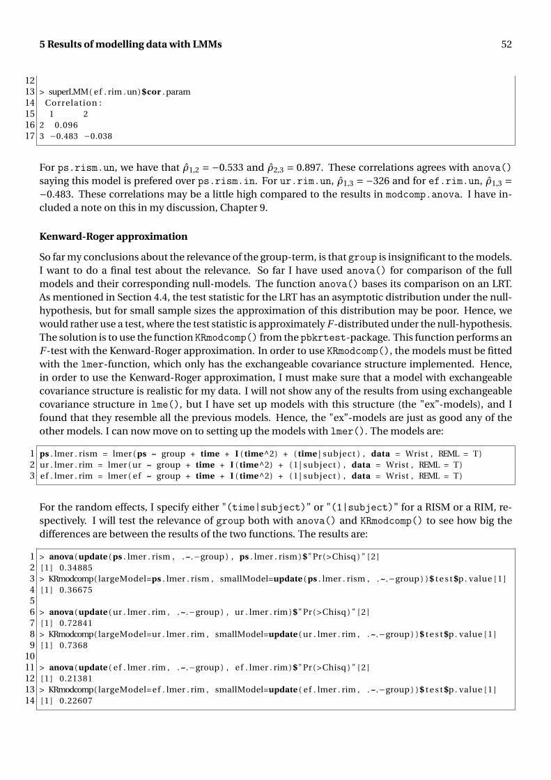
5 Results of modelling data with LMMs 52
1213 > superLMM( ef . rim . un) $cor . param14 Correlation :15 1 216 2 0.09617 3 −0.483 −0.038
For ps.rism.un, we have that ρ1,2 = −0.533 and ρ2,3 = 0.897. These correlations agrees with anova()saying this model is prefered over ps.rism.in. For ur.rim.un, ρ1,3 = −326 and for ef.rim.un, ρ1,3 =−0.483. These correlations may be a little high compared to the results in modcomp.anova. I have in-cluded a note on this in my discussion, Chapter 9.
Kenward-Roger approximation
So far my conclusions about the relevance of the group-term, is that group is insignificant to the models.I want to do a final test about the relevance. So far I have used anova() for comparison of the fullmodels and their corresponding null-models. The function anova() bases its comparison on an LRT.As mentioned in Section 4.4, the test statistic for the LRT has an asymptotic distribution under the null-hypothesis, but for small sample sizes the approximation of this distribution may be poor. Hence, wewould rather use a test, where the test statistic is approximately F -distributed under the null-hypothesis.The solution is to use the function KRmodcomp() from the pbkrtest-package. This function performs anF -test with the Kenward-Roger approximation. In order to use KRmodcomp(), the models must be fittedwith the lmer-function, which only has the exchangeable covariance structure implemented. Hence,in order to use the Kenward-Roger approximation, I must make sure that a model with exchangeablecovariance structure is realistic for my data. I will not show any of the results from using exchangeablecovariance structure in lme(), but I have set up models with this structure (the "ex”-models), and Ifound that they resemble all the previous models. Hence, the "ex”-models are just as good any of theother models. I can now move on to setting up the models with lmer(). The models are:
1 ps . lmer . rism = lmer ( ps ~ group + time + I ( time^2) + ( time | subject ) , data = Wrist , REML = T)2 ur . lmer . rim = lmer ( ur ~ group + time + I ( time^2) + ( 1 | subject ) , data = Wrist , REML = T)3 ef . lmer . rim = lmer ( ef ~ group + time + I ( time^2) + ( 1 | subject ) , data = Wrist , REML = T)
For the random effects, I specify either "(time|subject)” or "(1|subject)” for a RISM or a RIM, re-spectively. I will test the relevance of group both with anova() and KRmodcomp() to see how big thedifferences are between the results of the two functions. The results are:
1 > anova ( update ( ps . lmer . rism , . ~.−group ) , ps . lmer . rism ) $"Pr( >Chisq ) " [ 2 ]2 [ 1 ] 0.348853 > KRmodcomp( largeModel=ps . lmer . rism , smallModel=update ( ps . lmer . rism , . ~.−group ) ) $ t e s t $p . value [ 1 ]4 [ 1 ] 0.3667556 > anova ( update ( ur . lmer . rim , . ~.−group ) , ur . lmer . rim ) $"Pr( >Chisq ) " [ 2 ]7 [ 1 ] 0.728418 > KRmodcomp( largeModel=ur . lmer . rim , smallModel=update ( ur . lmer . rim , . ~.−group ) ) $ t e s t $p . value [ 1 ]9 [ 1 ] 0.7368
1011 > anova ( update ( ef . lmer . rim , . ~.−group ) , ef . lmer . rim ) $"Pr( >Chisq ) " [ 2 ]12 [ 1 ] 0.2138113 > KRmodcomp( largeModel=ef . lmer . rim , smallModel=update ( ef . lmer . rim , . ~.−group ) ) $ t e s t $p . value [ 1 ]14 [ 1 ] 0.22607

5 Results of modelling data with LMMs 53
All tests agree, that group is insignificant to the models. Furthermore, notice that the p-values fromanova() are very similar to the p-values from KRmodcomp(). This tells us, that we can trust the resultsfrom anova() even though they are based on asymptotic results.
5.5 Conclusion
No matter the covariance structure, there were problems wrt. the normality assumption of either therandom intercepts, slopes or the residuals, and some problems wrt. the homoscedasticity assumptionfor the models of the ex/flex-movement. Assuming these problems could be solved from having a muchlarger sample to analyse, I end this chapter with the conclusion that there is no evidence to reject H main
0 .But perhaps it would be better to use a model that does not require having to satisfy any assumptions.In the following chapter, I present a way to do this by using generalized estimating equations, and inChapter 7, the results of this approach are presented.
5.6 Source code: superLMM()
1 superLMM = function (mod, ass = NULL, i s = NULL) {2 par (mar = c ( 4 . 5 , 4 . 5 , 2 , 1 ) , lwd = 2 , cex . lab = 2 , cex . axis = 1 . 5 , cex . main = 2)34 ## P o s i t i v e semi−d e f i n i t5 V0 = getVarCov (mod, type = " marginal " , individual = 1)$id016 R0 = getVarCov (mod, type = " conditional " , individual = 1)$id017 Sigma = getVarCov (mod, type = "random . e f f e c t s " )8 c l i s t = l i s t (V0 , R0 , Sigma )9 psd = c ( )
10 for ( i in 1 : 3 ) {11 i f ( matrixcalc : : i s . symmetric . matrix ( c l i s t [ [ i ] ] ) ) { psd [ i ] = matrixcalc : : i s . p o s i t i v e . semi .
d e f i n i t e ( c l i s t [ [ i ] ] ) }12 else i f ( ! matrixcalc : : i s . symmetric . matrix ( c l i s t [ [ i ] ] ) ) {13 X = ( t ( c l i s t [ [ i ] ] ) + c l i s t [ [ i ] ] ) / 214 psd [ i ] = matrixcalc : : i s . p o s i t i v e . semi . d e f i n i t e (X)15 }16 }17 m. vcov = matrix ( psd , ncol = 3) ; colnames (m. vcov ) = c ( "V0" , "R0" , "Sigma" )1819 ## Relevance of " group "20 a1 = matrix ( c ( anova (mod) $"p−value " ) , ncol = 1 , nrow = 4)21 rownames( a1 ) = rownames( anova (mod) ) ; colnames ( a1 ) = "p−value "22 a2 = anova ( update (mod, . ~.−group , method = "ML" ) , update (mod, method = "ML" ) ) $"p−value " [ 2 ]23 i n t = i n t e r v a l s (mod, which = " f ixed " ) [ 1 ] $ f ixed [ , 1 : 3 ]2425 ## Association parameters26 cor . param = mod$modelStruct$corStruct2728 ## Assumptions29 ass . matrix = matrix ( c ( 0 , 0 , 0 ) , ncol = 3)30 colnames ( ass . matrix ) = c ( " Bart " , "Leve" , "Shap" ) ; rownames( ass . matrix ) = "p−value "31 rism = dim(mod$ c o e f f i c i e n t s $random$subject ) [ 2 ]32 i f ( ! i s . null ( ass ) ) {33 i f ( ass == 1) {34 i f ( ( rism == 1) | | ( rism == 2 && i s == " I " ) ) {35 layout ( matrix ( c ( 1 , 1 , 2 , 3 ) , 2 , 2 , byrow = T) )36 col = c ( rep (2 ,28) , rep ( "goldenrod1" , 28) , rep ( " chartreuse4 " , 27) )

5 Results of modelling data with LMMs 54
37 plot (mod$ c o e f f i c i e n t s $random$subject [ , 1 ] , col = col , cex = 0 . 5 , ylab = " Intercepts " ,xlab = " Patient index " )
38 car : : qqp(mod$ c o e f f i c i e n t s $random$subject [ , 1 ] , ylab = " Intercepts " , xlab = "Normquantiles " , main = " " , cex = 0 . 5 )
39 h i s t (mod$ c o e f f i c i e n t s $random$subject [ , 1 ] , probabi l i ty = T , 50 , xlab = " Intercepts " , main= " " )
40 l i n e s ( density (mod$ c o e f f i c i e n t s $random$subject [ , 1 ] ) , lwd = lwd , col = 2)4142 ass . matrix [ 1 , ] = c ( b a r t l e t t . t e s t (mod$ c o e f f i c i e n t s $random$subject [ , 1 ] , Wrist$group [ which (
Wrist$time==0) ] ) $p . value ,43 car : : leveneTest (mod$ c o e f f i c i e n t s $random$subject [ , 1 ] , Wrist$group [
which ( Wrist$time==0) ] ) $"Pr( >F) " [ 1 ] ,44 shapiro . t e s t (mod$ c o e f f i c i e n t s $random$subject [ , 1 ] ) $p . value )45 }46 i f ( rism == 2) {47 i f ( i s == "S" ) {48 layout ( matrix ( c ( 1 , 1 , 2 , 3 ) , 2 , 2 , byrow = T) )49 col = c ( rep (2 ,28) , rep ( "goldenrod1" , 28) , rep ( " chartreuse4 " , 27) )50 plot (mod$ c o e f f i c i e n t s $random$subject [ , 2 ] , col = col , cex = 0 . 5 , ylab = " Slopes " , xlab
= " Patient index " )51 car : : qqp(mod$ c o e f f i c i e n t s $random$subject [ , 2 ] , ylab = " Slopes " , xlab = "Norm quantiles "
, main = " " , cex = 0 . 5 )52 h i s t (mod$ c o e f f i c i e n t s $random$subject [ , 2 ] , probabi l i ty = T , 50 , xlab = " Slopes " , main =
" " )53 l i n e s ( density (mod$ c o e f f i c i e n t s $random$subject [ , 2 ] ) , lwd = lwd , col = 2)5455 ass . matrix [ 1 , ] = c ( b a r t l e t t . t e s t (mod$ c o e f f i c i e n t s $random$subject [ , 2 ] , Wrist$group [
which ( Wrist$time==0) ] ) $p . value ,56 car : : leveneTest (mod$ c o e f f i c i e n t s $random$subject [ , 2 ] , Wrist$group [
which ( Wrist$time==0) ] ) $"Pr( >F) " [ 1 ] ,57 shapiro . t e s t (mod$ c o e f f i c i e n t s $random$subject [ , 2 ] ) $p . value )58 }59 }60 }6162 i f ( ass == 2) {63 layout ( matrix ( c ( 1 , 1 , 2 , 3 ) , 2 , 2 , byrow = T) )64 col2 = c ( rep (2 ,3 * 28) , rep ( "goldenrod1" ,3 * 28) , rep ( " chartreuse4 " ,3 * 27) )65 plot (mod$residuals [ , 2 ] , ylab = " Residuals " , main = " " , cex = 0 . 5 )66 for ( i in seq (1 ,249 ,3) ) { l i n e s ( c ( i : ( i +2) ) ,mod$residuals [ i : ( i +2) , 2 ] , col = col2 [ i ] ) }67 car : : qqp(mod$residuals [ , 2 ] , ylab = " Residuals " , xlab = "Norm quantiles " , main = " " , cex =
0 . 5 )68 h i s t (mod$residuals [ , 2 ] , probabi l i ty = T , 50 , xlab = " Residuals " , main = " " )69 l i n e s ( density (mod$residuals [ , 2 ] ) , col = 2)7071 ass . matrix [ 1 , ] = c ( b a r t l e t t . t e s t (mod$residuals [ , 2 ] , Wrist$subject ) $p . value ,72 car : : leveneTest (mod$residuals [ , 2 ] , Wrist$subject ) $"Pr( >F) " [ 1 ] ,73 shapiro . t e s t (mod$residuals [ , 2 ] ) $p . value )74 }75 }7677 i f ( i s . null ( ass ) ) { out = l i s t ( vcov = m. vcov , group = l i s t ( anova1 = a1 , anova2 = a2 , i n t e r v a l s =
i n t ) , cor . param = cor . param) ; out }78 else79 print ( ass . matrix )80 }

6 | Generalized Estimating Equations
Generalized estimating equations models (GEE models for short) are an extension of the generalizedlinear models (GLMs for short). GLMs are fixed effects models, which assumes all observations are in-dependent of each other. Hence, GLMs are not suited for longitudinal data in most cases. Extendingthe GLM by specifying a correlation structure among observations on the same subject, we get the GEEmodel. The correlation structure is equivalent to R0 in the LMM. In Chapter 2, when testing the as-sumptions on the data, I had problems identifying the data as Gaussian. In Chapter 4, I worked underthe assumption, that the data was Gaussian as it seemed the most fitting distribution. Perhaps it wouldbe better not to make any such assumptions. An advantage of the GEE model over the LMM is that ituses quasi-likelihood. This means that the full likelihood of the data is not specified, hence no assump-tions on the distribution of the data are necessary.
To understand the setup in the GEE model, it is useful to review GLMs. I will therefore start this chapteroff with a quick run-through of the GLM before presenting the GEE model.
6.1 Generalized linear models
This section is based on [2], [7] and [12].
The GLM is an extension of the general linear model (LM for short). For a specific link function and vari-ance function, the GLM reduces to an LM. The assumptions in the LM are, that the response is Gaussian,the relationship between the response and the covariates is linear, and the variance of the response doesnot depend on the mean. In the GLM, the response does not have to be Gaussian. It just has to have adistribution from the exponential family. The most popular distributions in the exponential family arethe Gaussian, Binomial, Poisson and Gamma distributions. And the variance is actually a function ofthe mean. No matter the distribution, the density of the response can be written in the following form:
Definition 6.1 (Density for the exponential (dispersion) family) Let Y = [Y1 · · · YN
]Tbe a ran-
dom vector, where the Yi ’s are iid. with a distribution from the exponential family. The marginaldensities are then
f (yi ;θi ,φ) = h(yi ,φ
)exp
(yiθi −b(θi )
φ
), (6.1)
where φ is called the dispersion parameter, which may be known or unknown, θ is called the canon-ical parameter, and h(·) and b(·) are functions that depend on the distribution.
Example 2 shows how the density from a Binomially distributed random variable can be written in theform (6.1).
Example 2 In this example, I will show how a probability mass function (the discrete equivalent of thedensity function) can be written in the form (6.1). Let X be a Binomially distributed random variable,i.e. X ∼ Bi n(n,π). The probability mass function for X is defined as
p(x) =(
n
x
)πx(1−π)n−x , x = 0,1, . . . ,n.
We can ignore the subscripts in Equation (6.1), as X is a univariate random variable.

6 Generalized Estimating Equations 56
Rewritting p(x), it becomes
p(x) =(
n
x
)exp
(log
(πx(1−π)n−x)) =
(n
x
)exp
(x logπ+ (n −x) log(1−π)
)=
(n
x
)exp
(x
(log(π)− log(1−π)
)+n log(1−π)) =
(n
x
)exp
(x log
( π
1−π)+n log(1−π)
)= h(x)exp(xθ−b(θ)) ,
where h(x) = (nx
), θ = log
(π
1−π), b(θ) =−n log(1−π), and where φ is ignored as φ= 1 for this distribution.
ä
Linear predictor, link function and variance function
Three things are needed in specifying the GLM; the linear predictor, the link function and the variancefunction. The linear predictor, ηi , is a linear combination of the covariates
ηi = xTi β,
where xi is the vector of explanatory variables for subject i . The linear predictor is independent of thedistribution of the data. Let µi = E[Yi ]. The link function, g (·), is
g (µi ) = ηi .
Thus, the mean value is not a linear combination of the covariates (like we have with the general linearmodel), but instead it is assumed that the mean value is a function of the linear predictor, i.e.
µi = g (ηi )−1 = g (xTi β)−1.
Both µi and ηi are functions ofβ, and one ought to write µi (β) and ηi (β) to emphasize this. For the easeof notation, I will not do that. Each distribution has its own canonical link function shown below:
Distribution Gaussian Binomial Poisson Gammag (µi ) µi logit(π) log(µi ) 1
µi
The link function specifies how the covariates relate to the mean of the response. When working with,say, Gaussian data one is not restricted to only using g (µi ) = µi . One can choose which ever link func-tion that seems suitable for the data. Hence, the link function cannot be thought of as being dependenton the distribution of the data.
To find the variance function, we will need the mean and variance of Yi :
E[Yi ] =µiA.20= b′(θi ) and Var[Yi ]
A.20= φb′′(θi ).
Isolating θi in the expression of E[Yi ], we get
θi = b′(µi )−1. (6.2)
Inserting this into Var[Yi ], we see how the variance becomes a function of the mean:
Var[Yi ] =φb′′ (b′(µi )−1)=φV (µi ), (6.3)

6 Generalized Estimating Equations 57
where V (µi ) is the variance function. Each distribution has its own variance function shown below:
Distribution Gaussian Binomial Poisson GammaV (µi ) 1 π(1−π) µi µ2
i
The choice of variance function specifies the distribution of the data. This means that, unlike g (·), onedoes not have the freedom of choice. The GLM reduces to an LM if V (µi ) = 1 and g (µi ) = µi . Thedispersion parameter accounts for any excess variation not included by V (·). For instance, for a randomvariable X ∼ N
(µ,σ2
), as V (µ) = 1, this means that φ must be σ2 to account for the variation in X .
Example 3 In this example, I will show, that E[Yi ] = b′(θi ) and Var[Yi ] = φb′′(θi ) agrees with the meanand variance of the random variable from Example 2. For X ∼ Bi n(n,π), the mean and variance areE[X ] = nπ and Var[X ] = nπ(1−π). In Example 2, b(θ) =−n log(1−π) and θ = log
(π
1−π). In order to take
the derivative of b(·) wrt. θ, I will need to write b(·) with θ featured in its expression. I will do this byisolation π in the expression for θ:
θ = log( π
1−π)
⇔ π
1−π = exp(θ) ⇔ π= exp(θ)−πexp(θ) ⇔ π(1+exp(θ)
)= exp(θ)
⇔ π= exp(θ)
1+exp(θ).
I will now show that b′(θ) = E[X ]:
b′(θ) =− d
dθn log
(1− exp(θ)
1+exp(θ)
)= − d
dθn log
(1
1+exp(θ)
)= d
dθn log
(1+exp(θ)
)= n
1
1+exp(θ)exp(θ) = nπ = E[X ] .
Next, I will show that b′′(θ) = Var[X ]:
b′′(θ) = d
dθb′(θ) = d
dθn
exp(θ)
1+exp(θ)= n
exp(θ)(1+exp(θ)
)−exp(θ)2(1+exp(θ)
)2
= nexp(θ)
1+exp(θ)
(1+exp(θ)
1+exp(θ)− exp(θ)
1+exp(θ)
)= nπ(1−π) = Var[X ] .
ä
Estimating equations
Having specified the linear predictor, the link function, and the variance function, one can estimate thecoefficients,β, by solving an estimating equation. Let `i and Si be the log-likelihood and score function,respectively, of Equation (6.1) for the i th subject. By the chain rule, we have that
Si = ∂`i
∂µi= ∂`i
∂θi× ∂θi
∂µi
A.21= yi −b′(θi )
φV (µi ). (6.4)
Thus∂`i
∂β j= ∂`i
∂µi× ∂µi
∂β j
(6.4)= yi −b′(θi )
φV (µi )× ∂µi
∂β j.

6 Generalized Estimating Equations 58
The estimating equations thus becomes
S(β) =N∑
i=1
∂`i
∂β=
N∑i=1
(∂µi
∂β
)T yi −b′(θi )
φV (µi )=
N∑i=1
(∂µi
∂β
)T
Var[Yi ]−1 (yi −µi ) = 0. (6.5)
Note that S(β) was derived using the density of the data. If the distribition is unknown, the density can-not be defined, and if the distribution does not belong to the exponential family, the likelihood functioncannot be defined by Equation (6.1). Thus, the GLM fails as a possible approach for modelling the data.
I will now present a different approach of estimating β, that does not need the density or knowledge ofthe distribution of the data. Instead of Si , we will define a function that satisfy all the same properties asSi , i.e.
E[Si ] = 0 and Var[Si ] =−E
[∂Si
∂µi
].
Let that function beqi = q(µi , yi ) = yi −µi
φV (µi ).
It is shown in A.22, that qi satisfy the properties. As for the expression for qi , it is chosen because it isequal to the expression for Si (Equation (6.4)) with the important distinction that b′(θi ) requires knowl-edge of the distribution of yi in order to be calculated, whereas µi in qi does not. As qi mimics a properscore function, the integral of qi will mimic a proper log-likelihood. The log quasi-likelihood functionfor subject i is thus defined as
Qi =Q(µi , yi ) =∫ µi
yi
yi − ti
φV (ti )d ti .
The log quasi-likelihood for all subjects is
Q =Q(µ,y) =N∑
i=1Qi =
N∑i=1
∫ µi
yi
yi − ti
φV (ti )d ti .
Differentiating Qi wrt. µi of course just gives qi . As g (µi ) = xTi β does not depend on a specific distribu-
tion, we can differentiate Qi wrt. β:
∂Qi
∂β= ∂Qi
∂µi× ∂µi
∂β= yi −µi
φV (µi )× ∂µi
∂β.
We now get new estimating equations (also called maximum quasi-likelihood equations):
S(β) = ∂Q
∂β=
N∑i=1
∂Qi
∂β=
N∑i=1
yi −µi
φV (µi )× ∂µi
∂β=
N∑i=1
(∂µi
∂β
)T
Var[Yi ]−1 (yi −µi ) = 0. (6.6)
Equations (6.5) and (6.6) may look identical, but they are not in the sense that they are derived in differ-ent ways. Equation (6.5) can only be derived when the density is know and the distribution belongs tothe exponential family. Equation (6.6) can be derived regardless of the distribution of data or whetherthe density is known; we only need to specify how the mean depend on the covariates through the linkfunction, and how the variance variates as a function of the mean, i.e. the variance function, in order toestimate β. Solution of Equation (6.6) are called quasi-likelihood estimates.

6 Generalized Estimating Equations 59
6.2 GEE models
This section is based on [2], [12] and [13].
In a data set with more than one observation per subject, it would be very likely that observations onthe same subject are somehow correlated. Nothing in the specification of the GLM takes this into ac-count. Hence, a GLM with multiple responses per subject will only be a sensible model in the case, thatno observations on the same subject are correlated. The GEE model18 is an extension of the GLM thatdoes take into account observations on the same subject possibly being correlated. The GEE model usesa quasi-likelihood approach and thus does not require a specification of the underlying distribution ofthe response. The setup resembles the GLM, only now we have a multidimensional response per sub-ject instead of a univariate response, and in addition to the linear predictor, the link function and thevariance function, we also have to specify a correlation structure.
Let yi be the vector of responses from the i th subject, where the response, yi j , is taken at timepoint j .The linear predictor, link function and variance function are
ηi j = xTi jβ,
g (µi j ) = ηi j ,
Var[Yi j
]=φV (µi j ), (6.7)
where xi j is the vector of covariates for subject i at timepoint j . Additionally, the correlation structure ofthe repeated measurements must be specified. It is assumed that the number of timepoints is fixed. Letthat number be n. Subjects do not need to have been measured at all n timepoints, but for the sake ofsimplicity (and because it is the case with my data), I will assume they were. The correlation matrix forsubject i is denoted by Ri , and it is assumed it depends on a vector of association parameters, a, hencewe write Ri (a). Just like in the LMM, we have that all subjects have the same covariance matrix, hencewe can write Ri (a) = R0(a). The association parameters are the same for all subjects. The correlationstructure can be expressed in several ways that the reader may recognize from Section 4.3:
• Independence: R0(a) = In×n . This rarely makes sense for longitudinal data, however.
• Exchangeable: R0(a) j k = ρ j k ={
1, j = k
a, j 6= k.
• Autoregression: R0(a) j k = ρ j k = a| j−k|, a ∈]0,1[. This is usually the most popular choice for longi-tudinal data.
• Unstructured: R0(a) j k = ρ j k = a j k . This is the most efficient choice when n is a small number.
Other choices are also available. Note, that if R0(a) = In×n , the GEE models assumes that there is nowithin-subject correlation and thus reduces to a GLM.
6.2.1 GEE estimation of parameters
Let Ai = diag{√
V (µi j )}
j=1,...,n . The covariance matrix for yi is defined as
Vi (a) =φAi R0(a)Ai . (6.8)
18The term "model” is used a little loosely when speaking of the GEE model. As it uses a quasi-likelihood and not a properlikelihood, we do not actually have any model. Nevertheless, for simplicity, I will call it a model.

6 Generalized Estimating Equations 60
The coefficients β are estimated by solving the estimating equations
S(β) =N∑
i=1
∂µTi
∂βVi (a)−1(yi −µi ) = 0. (6.9)
In order to solve Equation (6.9), we must find Vi (a), meaning we must find a and φ. These parametersare unknown and must be estimated.
Finding a
Let
r j k = (Yi j −µi j )(Yi k −µi k )
φ√
V (µi j )V (µi k ), ∀i
which is a function of β and has mean
E[r j k
] A.23= ρ j k = Corr[Yi j ,Yi k
].
Gathered in one vector, we have r = [r12,r13, . . . ,rn−1,n
] ∈R n(n−1)2 ×1. Let
ρ(a) = E[r] = [ρ12,ρ13, . . . ,ρn−1,n
],
which is a function of a because ρ j k is a function of a. Then a is estimated by the estimating equations
∂ρ(a)
∂aW−1 (
r−ρ(a))= 0, (6.10)
where W is the covariance matrix for r, typically specified as diag{Var
[r j k
]}. Notice how the form of this
estimating equation is the same as in Equation (6.9); a product between the derivative of the mean, thecovariance function and the raw residuals.
Findingφ
Isolating φ in Equation (6.7), we get
φ(6.7)= Var
[Yi j
]V (µi j )
= E[(Yi j −µi j )2
]V (µi j )
.
When µi j is estimated, we can insert it to get an estimate of φ. But, the estimate for φ must hold for allobservations. Hence, if we calculate the Pearson residuals
εi j =yi j − µi j√
Vi (a) j j,
and sum over these corrected for the degrees of freedom, we get the estimate of φ
φ= 1
N −p
N∑i=1
n∑j=1
ε2i j . (6.11)
Solving Equation (6.9) wrt. βmeans that β is dependent on the current estimate of a. As r is a function ofβ, a is dependent on the current estimate of β. This means that the GEE estimator of β is found throughan iterative algorithm:

6 Generalized Estimating Equations 61
Algorithm 6.2 (Algorithm for the GEE estimator) mellemrum
i. Initialize β, e.g. as the coefficients from a GLM.
ii. Using β, estimate R0(a) by inserting a estimated from solving Equation (6.10), and estimate φby Equation (6.11).
iii. Using a and φ, estimate Vi (a) by Equation (6.8).
iv. Using Vi (a), estimate β by solving Equation (6.9).
Repeat step ii.-iv. until convergence.
I want to know whether or not it is a garantee, that Algorithm 6.2 converges, and if different initial β’swill lead to the same final GEE estimator. Unfortunately, I have found no sources that says anythingabout this matter, so perhaps it is simply unknown. The function geeglm() from the geepack-packageis one of the functions one might use for correlated GLM-type data, such as Wrist. I have looked atthe source code for geeglm() thinking that if non-convergence was a possibility, then it must be imple-mented in the function, that the iterations should stop when reaching a certain limit. No such thing wasimplemented. This leads me to think, that convergence is always garanteed, but I cannot be sure. Ingeeglm(), it is implemented that the initial β is the coefficients from modelling the data with a GLM,just like step i. in Algorithm 6.2. I believe that the initial β is chosen like this as it will lower the num-ber of iterations, because the coefficients from the GLM usually are not that far from the GEE estimator.Coincidentally, unrelated to this report, I have coded a function called my_gee() in R based on this algo-rithm. The function, my_gee(), was intended as a homemade version of geeglm(). I will now, throughan example, argue that my_gee(), and thus Algorithm 6.2, always returns the same GEE estimator nomatter the initial β.
Example 4 The data set I will be using is Orthodont from the nlme-package. It consists of 27 boys andgirls. At the ages 8, 10, 12 and 14, the change in an orthodontic measurement (distance from pituitary topterygomaxillary fissure) have been recorded. The data consists of four variables; distance, age, Sexand Subject. Below, the first eight rows of the data are shown:
1 > head ( Orthodont , 8)2 distance age Subject Sex3 1 26.0 8 M01 Male4 2 25.0 10 M01 Male5 3 29.0 12 M01 Male6 4 31.0 14 M01 Male7 5 21.5 8 M02 Male8 6 22.5 10 M02 Male9 7 23.0 12 M02 Male
10 8 26.5 14 M02 Male
I will now model the response, distance, with both geeglm() and my_gee(). Through the argumentinit.beta in my_gee(), I specify nine different initial β’s to see what GEE estimator it will result in andhow many iterations are used. The initial β’s will be vectors where all entries are equal to init.beta. Inmy_gee() only g (µi ) = µi and V (µi ) = 1 is implemented, and init.beta is per default the coefficientsfrom a GLM, just like in geeglm(). The nine values of init.beta are
ib = c(NULL, -5000, -777, -0.3, 0, 0.00005, 4, 100, 1234, 5678),

6 Generalized Estimating Equations 62
where NULL is the default setting. I have made a for-loop that runs through these values and gathersthe GEE estimators in a matrix, coefs, together with the number of iterations used. The model withgeeglm() and the models with my_gee() are shown below, where ib takes the nine values one at a time:
1 m. geeglm = geeglm ( distance ~ age + Sex , id = Subject , data = Orthodont , family = " gaussian " ,c o r s t r = " unstructured " )
2 m.my_gee = my_gee ( distance ~ age + Sex , id = Orthodont$Subject , data = Orthodont , c o r s t r = "unstructured " , i n i t . beta = ib [ i ] )
Below, in coefs, the GEE estimators are listed in the order mentioned above. This means that the firstrow in coefs is the GEE estimator, we get when initializing β with the coefficients from a GLM. Thisestimator is not perfectly equal to that of m.geeglm, but the differences are very small. We see that evenwith very big differences in the initial β’s, the GEE estimator is always the same. Only the number ofiterations change. Thus, I believe that Algorithm 6.2 always returns the same GEE estimator no matterthe initial β.
1 > m. geeglm$ c o e f f i c i e n t s2 ( Intercept ) age SexFemale3 17.696016 0.6597990 −2.223226045 > coefs6 ib ( Intercept ) age SexFemale i t e r a t i o n s7 [ 1 , ] NULL 17.59809 0.6691337 −2.255985 138 [ 2 , ] −777.00000 17.59809 0.6691337 −2.255985 139 [ 3 , ] −0.30000 17.59809 0.6691337 −2.255985 12
10 [ 4 , ] 0.00000 17.59809 0.6691337 −2.255985 1211 [ 5 , ] 0.00005 17.59809 0.6691337 −2.255985 1212 [ 6 , ] 4.00000 17.59809 0.6691337 −2.255985 1213 [ 7 , ] 100.00000 17.59809 0.6691337 −2.255985 1314 [ 8 , ] 1234.00000 17.59809 0.6691337 −2.255985 1315 [ 9 , ] 5678.00000 17.59809 0.6691337 −2.255985 13
ä
Much like the maximum likelihood estimator from Chapter 4, the GEE estimator, β, is asymptoticallyNp
(β, I(β)−1
)-distributed, where
I(β)−1 =−E
[∂
∂βTS(β)
]=
N∑i=1
∂µTi
∂βVi (a)−1 ∂µi
∂βT. (6.12)
Upon convergence, we would like to interpret on the effects related to the groups. Ideally, we would setup some models and then do comparisons using LRTs. But as β are estimates obtained using quasi-likelihood, and not the usual likelihood, no LRTs can be performed. Luckily, we can still do a Wald testto determine whether βi = 0. Thus we rely on inference aboutβ. Regardless of whether Vi (a) is specifiedcorrectly, β will be a consistent estimator of β. Hence, whether or not β is consistent cannot be usedas an argument to choose one correlation structure over an other. Instead, we can look at the standarderrors for β. For this, we will need the covariance of β. The standard errors are the squared diagonalelements in the covariance matrix. There are two ways to estimate Cov
[β
]:
• The model based estimate:Cov
[β
]M
(6.12)= I(β).

6 Generalized Estimating Equations 63
If the mean value and correlation structure are specified correctly, then Cov[β
]M is a consistent es-
timator of Cov[β
]. The model based estimate yields a close approximation of the standard errors
of β provided Vi (a) is a close approximation of the true underlying covariance.
• The empirical estimate:
Cov[β
]E = I(β)
(N∑
i=1
∂µTi
∂βVi (a)−1Cov[Yi ]Vi (a)−1 ∂µi
∂βT
)I(β).
Even if the correlation structure is misspecified, Cov[β
]E is a consistent estimator of Cov
[β
]. The
empirical estimate is also known as the "robust” estimate because it is always consistent and be-cause it yields correct standard errors of β for large sample sizes, despite Vi (a) being misspecified.
Clearly, if Cov[Yi ] is specified correctly, so that Cov[Yi ] = Vi (a), then Cov[β
]E = Cov
[β
]M. This means,
that when testing different covariance structures, the one that fits data best, will be the one that reducesthe difference between Cov
[β
]E and Cov
[β
]M. In practice, Cov[Yi ] is replaced by (yi − µi )(yi − µi )T .
The GLM does not take into account that observations may be correlated. But how much exactly doesthat influence the model? And how big does the difference between Cov
[β
]M and Cov
[β
]E have to be
for it to be obvious, that the chosen covariance structure is unrealistic for the data? I will try to answerthese questions in Example 5.
Example 5 The example is based on the data set respitory from the package HSAUR2. I will be using asubset of respitory in which I have made a few changes. The new data set is called resp and consistsof 444 observations on 111 patients (4 observations per patient). The patients were observed for theirrespitory status, which was either "poor” or "good”. Below are the first 10 rows of the data:
1 > head ( resp , 10)2 centre group gender age month subject baseline status3 112 1 placebo female 46 1 1 poor 04 223 1 placebo female 46 2 1 poor 05 334 1 placebo female 46 3 1 poor 06 445 1 placebo female 46 4 1 poor 07 113 1 placebo female 28 1 2 poor 08 224 1 placebo female 28 2 2 poor 09 335 1 placebo female 28 3 2 poor 0
10 446 1 placebo female 28 4 2 poor 011 114 1 treatment female 23 1 3 good 112 225 1 treatment female 23 2 3 good 1
The data consists of 8 variables:
• baseline: the patients’ status at the start of the study,
• month: once a month in the next four following months, their respitory status was registered. Thisvariable indicates which month, we are at,
• status: the patients’ current status coded as "0” for "poor” and "1” for "good”,
• centre: the centre they were treated at, either 1 or 2,
• group: the patients were randomized into two treatment groups and were given either a placeboor treatment drug,

6 Generalized Estimating Equations 64
• gender: selfexplanatory,
• age: their age at the time the observation was registered ranging from 11 to 68 years, and
• subject: a factor identifying each patient.
The response variable is binary, so I will be using the link and variance function from the Binomial dis-tribution. I will set up a GLM and two GEE models; one with independence and one with unstructuredcorrelation structure. I will fit a logistic regression model to the data using glm(), and I will set up theGEE models with the function geeglm() from the package geepack. The setup of the geeglm-functionis fairly selfexplanatory as it resembles glm(). Only a few extra arguments are specified:
1 resp . glm = glm( status ~ centre + group + gender + baseline + age , family = "binomial " , data =resp )
2 resp . gee1 = geeglm ( status ~ centre + group + gender + baseline + age , family = "binomial " ,c o r s t r = "independence" , scale . f i x = T , id = subject , data = resp )
3 resp . gee2 = geeglm ( status ~ centre + group + gender + baseline + age , family = "binomial " ,c o r s t r = " unstructured " , scale . f i x = T , id = subject , data = resp )
Through the argument corstr, the correlation structure is specified, and the argument id is needed toseperate the observations according to subjects when estimating Vi (a), for instance. Through scale.fix,I tell the function whether φ should be estimated or fixed at the value 1. Only when there might be aproblem with overdispersion, do I want to estimate φ. That is not the case here, though:
1 > tapply ( resp$status , interaction ( resp$group , resp$month) , mean)2 placebo . 1 treatment . 1 placebo . 2 treatment . 2 placebo . 3 treatment . 3 placebo . 4 treatment . 43 0.49123 0.68519 0.38596 0.70370 0.45614 0.72222 0.43860 0.6296345 > tapply ( resp$status , interaction ( resp$group , resp$month) , var )6 placebo . 1 treatment . 1 placebo . 2 treatment . 2 placebo . 3 treatment . 3 placebo . 4 treatment . 47 0.25439 0.21978 0.24123 0.21244 0.25251 0.20440 0.25063 0.23760
The very first column
placebo.1
0.49123
shows that the mean for the placebo-group at the 1st timepoint is 0.49123. In these outputs, we see thatthere is not much difference between the means and variances of status at each of the timepoints forthe treatment groups. Hence, I fix φ at 1.
I have extracted the standard errors from all three models and gathered them in the matrix below foreasy comparison:
1 > SEmatrix2 glm gee1 .M gee1 . E d i f f . 1 gee2 .M gee2 . E d i f f . 23 ( Intercept ) 0.33765 0.33728 0.46033 −0.12305 0.47994 0.46128 0.018664 centre2 0.23957 0.23930 0.35682 −0.11752 0.33960 0.35480 −0.015205 grouptreatment 0.23684 0.23658 0.35078 −0.11420 0.33596 0.34945 −0.013496 gendermale 0.29467 0.29435 0.44320 −0.14886 0.41794 0.44365 −0.025717 baselinegood 0.24129 0.24102 0.35005 −0.10903 0.34337 0.34804 −0.004678 age 0.00886 0.00885 0.01300 −0.00415 0.01258 0.01291 −0.00033

6 Generalized Estimating Equations 65
First column is the standard errors of resp.glm. The next three columns are the model based standarderrors, the empirical standard errors and the difference between these, respectively, for resp.gee1. Thelast three columns are the same, but for resp.gee2.
As mentioned earlier, the GLM is just a GEE model with independence correlation structure, so it mayseem strange that glm and gee1.M are not identical. This is due to the algorithm geeglm() uses duringestimation. Had I used the function gee() from the package gee, I would have got identical results.However, glm and gee1.M are close enough, that we may proceed with geeglm(). Looking only at glm,there is no way to tell whether the model is a good fit for the data. It is a bit easier for the GEE modelsas we can compare the model based and the empirical standard errors, in order to conclude whetherthe model is any good. In the columns diff.1 and diff.2, it is clear that unstructured correlationsstructure is more realistic for the data, as diff.2 < diff.1 by about a factor of 10 per variable in themodels. To further underline resp.gee2 being the better model, the estimated association parameters,a, show that there indeed is a correlation between observations on the same subject19:
1 > resp . gee2$geese$alpha2 alpha . 1 : 2 alpha . 1 : 3 alpha . 1 : 4 alpha . 2 : 3 alpha . 2 : 4 alpha . 3 : 43 0.328 0.208 0.298 0.439 0.363 0.399
The correlations are not extremely high, but they are certainly not 0 either. In conclusion, in this exam-ple, we have seen that the GLM is an insufficient model, when the responses are multidimensionel. Andwe have seen how to use the standard errors to choose the more fitting correlation structure for the data.
ä
6.3 GEE vs. LMM
This section is based on [13].
In the GEE model, we estimateβ, so that we can say something about the population-averaged effect. Inthe LMM, we furthermore estimate the ui ’s, which enables us to "dig a little deeper” and say somethingabout the subject-specific effects.
! We want to know the effect of the treatment on each of the patients, and we want to use this todetermine whether there is a difference in the treatment groups. In that sense, we should use anLMM as we are interested in the subject-specific effects. But we could also formulate the goal ofthis report a little differently, so that it makes sense to use a GEE model. Stated in a different way,we want to know how well the patients react to Ibuprofen wrt. wrist mobility. We want to knowthe population-averaged effect of the treatment groups. This allows us to compare the groups.
The GEE model can only take into account one source of clustering. If the vocabulary test-examplefrom Chapter 4 had been extended to including several schools with several classes, we would also haveto take into account the within-school and within-class correlation. This is no problem for the LMMas it would account for these extra sources of variation by having a random effect for each source. Wecannot do that in the GEE model as no random effects are specified in the model. It is only through thecorrelation, R0(a), where the within-subject association among repeated measurements is incorporated,that we account for the population-averaged effects. So, a disadvantage of the GEE model is that wecannot use it if we have more than one source of random effects. And, obviously, if we are interested inthe subject-specific effects, the GEE model is no good.
19Some literature usesα instead of a, which is why "alpha” is in the output from R.

6 Generalized Estimating Equations 66
An advantage of the GEE model is that, as mentioned, even if the correlation is misspecified, both β andCov
[β
]E are still consistent estimators. The fact that the GEE model provides two covariance matrices
for β is helpful when choosing the better model according to covariance structure. Another advantageof the GEE model is, as mentioned also, that no assumptions on the distribution of the data is needed.Wrt. the residuals, there is no assumption of them being Gaussian with zero mean, but it does improveefficiency of β if this holds. Actually, if the mean and variance of the response is correctly specified, theresiduals will be Gaussian with zero mean.

7 | Results of modelling data with GEEs
In this chapter, I go through the results of modelling the response variables with GEE models as de-scribed in Chapter 6. The setup of this chapter is the same as in Chapter 5; first I will choose a functionto set up models. Then I will perform the analysis with the autoregressive, the unstructured and theindependence correlation structure, respectively, and I will end the analysis with a comparison of thethree sets of models to see which correlations structure is most realistic for the data. I will end the chap-ter with a conclusion of whether there is any significant difference between the treatment groups.
Choosing a function and a model
The packages geepack, gee and geeM offer the functions geeglm(), gee() and geem, respectively, forcreating a GEE model. The setup in the functions is nearly identical, and having tested these functionson my data, I find I get all the same results. The only differences are what is displayed in some of theoutputs, for instance, the output of summary() is a little different for each of the functions. Hence, itmakes no difference which function I choose, and as such, I will choose geeglm().
Next, I must decide whether φ should be estimated freely or fixed at 1. For this, I find the means andvariances across the groups at the three timepoints for each type of movement:
1 > tapply ( Wrist$ps , interaction ( Wrist$group , Wrist$time ) , mean)2 1.0 2.0 3.0 1.7 2.7 3.7 1.46 2.46 3.463 58.416 63.620 66.118 86.940 85.728 91.516 94.210 93.554 95.91445 > tapply ( Wrist$ps , interaction ( Wrist$group , Wrist$time ) , var )6 1.0 2.0 3.0 1.7 2.7 3.7 1.46 2.46 3.467 365.89 390.05 279.78 144.25 154.90 57.68 84.36 84.44 18.3289 > tapply ( Wrist$ur , interaction ( Wrist$group , Wrist$time ) , mean)
10 1.0 2.0 3.0 1.7 2.7 3.7 1.46 2.46 3.4611 31.952 38.166 33.828 71.238 68.222 77.403 93.860 89.605 92.4911213 > tapply ( Wrist$ur , interaction ( Wrist$group , Wrist$time ) , var )14 1.0 2.0 3.0 1.7 2.7 3.7 1.46 2.46 3.4615 152.65 253.14 202.52 362.75 406.50 258.38 407.92 212.50 327.231617 > tapply ( Wrist$ef , interaction ( Wrist$group , Wrist$time ) , mean)18 1.0 2.0 3.0 1.7 2.7 3.7 1.46 2.46 3.4619 22.426 29.311 27.920 66.028 69.634 71.771 87.150 92.058 89.4782021 > tapply ( Wrist$ef , interaction ( Wrist$group , Wrist$time ) , var )22 1.0 2.0 3.0 1.7 2.7 3.7 1.46 2.46 3.4623 127.50 319.69 170.19 132.36 443.08 245.07 102.44 238.74 280.13
The output of tapply() needs a quick explanation. The first column in the first tapply()
1.0
58.416
tells us, that the mean of ps for group 1 at the first timepoint (coded as 0) is 58.416. Hence, the first rowin the output refers to the groups (either 1, 2 or 3) at the timepoints (either 0, 7, or 46), and the secondrow is the mean for that group at that timepoint. Clearly, there is a difference between the means and the

7 Results of modelling data with GEEs 68
variances, which means that overdispersion could be a problem, and hence φ must be estimated freely.This is done by setting scale.fix = FALSE, which is the default setting in geeglm(), and as such, I willjust omit this argument in my models.
In Chapter 5, I reasoned that I should include a squared term of time in the model in order to achievelinearity between the response and the covariates. This time I will also include a squared term in themodels, which means the link function is just the identity, i.e. g (µi ) = µi = xT
i β. In geeglm() this isexpressed by family = gaussian(link = "identity"), in which I also specify the variance functionas belonging to the Gaussian family20. Like in Chapter 5, I will begin my analysis using autoregressivecovariance structure. The models are set up as follows (here only the model for ps is shown):
1 ps . gee . ar = geeglm ( ps ~ time + I ( time^2) + group , id = subject , data = Wrist , c o r s t r = " ar1 " ,family = gaussian ( link = " i d e n t i t y " ) )
The models for the uln/rad- and ex/flex-movements, ur.gee.ar and ef.gee.ar, are set up the ex-act same way only with ur and ef instead of ps. The autoregressive covariance structure is specifiedthrough corstr = "ar1". In the GEE model no random effects are specified, although one could viewthe argument id as being somewhat equivalent to the random-argument in lme().
7.1 Analysis using corstr = "ar1"
I will start off by making sure the models (henceforth termed the "ar”-models) are not overdispersed.They should not be, as φ have not been set to any fixed value. To check for overdispersion, we comparethe estimated dispersion (extracted from summary()) with what it ought to be according to the formulain Algorithm 6.2:
1
N −p
N∑i=1
n∑j=1
ε2i j .
These two dispersions can be extracted from my function superGEE() by superGEE()$dispersion.For easy comparison of all the models, I have gathered these two values of φ in a simple matrix, wherethe rows refer to the estimates form either the summary or the formula:
1 > phi . ar2 ps . gee . ar ur . gee . ar ef . gee . ar3 summary 171.80 284.11 221.464 formula 175.32 289.93 226.00
I deem these differences small enough that none of the "ar”-models are overdispersed.
Only two things need to be tested; whether group is relevant to the models and whether the residuals arehomoscedastic. As it would improve efficiency in the sense, that the mean and variance of the responsewill have been correctly specified, if the residuals are Gaussian with zero mean, I will also be testing this.To test the relevance of the treatment groups, I am using three Wald tests, all of which is implementedin superGEE(). The first Wald test is performed by anova() with just one input (the model, we want totest). This test tests the hypotheses
H0,1 : βtime = 0, H0,2 : βtime2 = 0, H0,3 : βgroup = 0.
The second test is also performed by anova(), but with two inputs; the model, we want to test, and the20I have tested other choices for the variance function, but only the one from the Gaussian family gave sensible results.

7 Results of modelling data with GEEs 69
corresponding null-model. Just like in Chapter 5, I am using the term "null-model” to mean a modelwithout the group-term and otherwise identical to the corresponding full model. This test is just theusual comparison of two models, only compared using a Wald statistic instead of AIC. The third test isthe result of using the function esticon() on the model. This function also performs a Wald test, buttests the hypotheses that
H0,1 : βtime = 0, H0,2 : βtime2 = 0, H0,3 : βgr.2 = 0, H0,4 : βgr.3 = 0,
and it also gives the 95%-confidence intervals for the estimated coefficients. Remember, if zero is con-tained in the interval, we can accept that the corresponding coefficient is zero. The results of the threeWald tests are:
1 > superGEE ( ps . gee . ar ) $group2 $anova13 p−value4 time 0.000005 I ( time^2) 0.000006 group 0.1438078 $anova29 [ 1 ] 0.14380
1011 $esticon12 p−value lower upper13 ( Intercept ) 0.00000 55.62940 65.6371314 time 0.00000 3.62623 4.6655715 I ( time^2) 0.00000 −0.08473 −0.0654116 group2 0.60576 −4.33137 7.4281317 group3 0.05838 −0.16581 9.51960
The third p-value from $anova1 and the p-value from $anova2 seem to be the same. Had I includedmore decimals, we would see, that they are very close, but not equal21 (this goes for all the models inthis chapter). The output shows that group is irrelevant to ps.gee.ar. The same goes for the modelsur.gee.ar and ef.gee.ar as seen in Table 4. In the table, I am including the p-values and confidenceintervals for group only, as these results are of most interest.
Table 4: Results of using superGEE()$group on the "ar”-models. The row for $anova1 are the p-values for group.The row for $anova2 are the p-values from the comparison of the model and the corresponding null-model. Therows for $esticon are the 95%-confidence intervals for βgr.2 and βgr.3, and the p-values for these coefficients.
superGEE()$groupur.gee.ar ef.gee.ar
$anova1 0.88083 0.09464
$anova2 0.88083 0.09464
$esticon βgr.2 ∈ [−6.64,6.93], 0.96712 βgr.2 ∈ [−0.61,11.53], 0.07793βgr.3 ∈ [−5.03,8.02], 0.65431 βgr.3 ∈ [−0.72,9.24], 0.09379
The results from superGEE()$group are unanimous; group is irrelevant to the models.
21I thought perhaps the p-values from $anova1 was a result of anova() one by one removing time, I(time)o2 and groupfrom the model, and then comparing the reduced model with ps.gee.ar. Upon investigation, I found that that is not so.

7 Results of modelling data with GEEs 70
Testing ps.gee.ar for homoscedasticity, I get the plots in Figure 16 and the following p-values:
1 > superGEE ( ps . gee . ar , t e s t = "homo" )2 Bart Leve3 0.00020 0.98368
id01 id08 id15 id22 id29 id36 id43 id50 id57 id64 id71 id78
−40
020
40
Subject
Res
idua
ls
●
●●
●
●●
●●
●
●
●
●
●●
●
●●
●
●
●
●
●
●
●
●
●
●
●
●
●
●
●
●●
●
●
●
●
●
●
●
●
●
●
●
●
●
●
●
●●
●
●
●
●●
●
●
●●
●
●
●
●
●
●●
●●
●
●
●
●
●●
●
●
●
●
●
●
●
●●●
●●
●
●
●
●
●
●
●
●●
●
●
●
●
●
●
●
●
●
●
●
●
●
●
●
●
●
●
●
●
●
●
●
●
●
●
●
●
●●
●
●
●
●
●
●
●
●
●
●
●
●●
●
●
●●●
●
●
●
●
●●
●●●
●
●
●●
●
●
●
●
●
●
●
●●
●●●
●
●
●
●
●
●
●
●
●
●
●
●
●
●
●●
●
●
●●
●
●●
●●
●
●
●
●
●
●
●
●
●
●●
●●
●
●●
●
●
●
●
●
●
●
●
●
●
●
●
●
●●
●
●
●
●
●
●
●
●●
●
●
●
●
●●
●
●
●
●
●
●
●●
●
0 50 100 150 200 250
−40
020
40
Index
Res
idua
ls
Figure 16: Top: Boxplots of each patients’ residuals. Bottom: Residuals vs. their index numbers. In both plots, red,yellow and green represent group 1, 2 and 3, respectively.
The top plot in Figure 16 is intended for detecting patterns in the residuals between the groups. It showsthat there is a slightly smaller spread in the residuals from group 3, but otherwise no obvious patternsthat seperate the groups. An unwanted pattern that could show non-homoscedasticity could perhapsbe, that the boxplots for, say, group 1 all tended to have maximum values far from the median. The bot-tom plot is intended for detecting patterns in the residuals for each patient. This plot was explained inChapter 5 (just before Figure 10), where an unwanted pattern could perhaps be each patient’s residualsforming a "U”-shape. The plot shows no obvious trend in each patient’s residuals. I see no reason not toassume homoscedasticity, eventhough the Bartlett test disagrees with the Levene’s test. This is likely doto the residuals not being Gaussian, which we see when testing for normality by
1 > superGEE ( ps . gee . ar , t e s t = "norm" )2 Shap3 1.463e−08
Figure 17 shows that, although being centered around zero, the residuals are not Gaussian according to

7 Results of modelling data with GEEs 71
the Q-Q plot. The histogram agrees less with the Shapiro-Wilk test. We cannot rule out that they maybe asymptotically Gaussian. For ur.gee.ar and ef.gee.ar, the residuals are homoscedastic, and theplots from are similar to Figure 16 (although for ef.gee.ar, it is groups 1 that has the smallest spread).Neither of the models have Gaussian residuals. The Q-Q plots for the models look a lot better than theone in Figure 17, but the histograms are not nearly as good as the one for ps.gee.ar. The problems withnormality could be due to the autoregressive structure not being the most fitting for the data.
−3 −2 −1 0 1 2 3
−40
−20
020
40
Norm quantiles
Res
idua
ls
●
●
●
●
●
●
●●●●
●●●
●●
●●●●
●●●
●●●●
●●●●●
●●●●
●●●●●●●●
●●●●●●●●●●●
●●●●●●●●●●●
●●●●●●●●●●●●●
●●●●●●●●●●
●●●●●●●●●●●●●●●
●●●●●●●●●●●
●●●●●●●●●●●●●●●●●●●●●●●●
●●●●●●●●●●●●●●●●●●●
●●●●●●●●●●●●
●●●●●●●●●●●●●●●●●●●●●●●●●●●●●●●
●●●●●●●●●●●
●●●●●●●
●●●●●●
●●●●●●●●
●●●
●●
●
●●
●●●●
●● ●
●
●
Residuals
Den
sity
−40 −20 0 20 40
0.00
0.02
0.04
0.06
Figure 17: Left: Q-Q plot of the residuals. Right: Histogram of the residuals with density curve (red line).
7.2 Analysis using corstr = "unstructured"
The models ps.gee.un, ur.gee.un and ef.gee.un are set up exactly like the "ar”-models, only withcorstr = "unstructured" used instead. I will refer to these models as the "un”-models. Once again,I am starting off by confirming that they are not overdispersed. Next, I move on to testing the relevanceof group. The results from superGEE()$group are shown in Table 5. These results show that group isirrelevant to the "un”-models.
Table 5: Results of using superGEE()$group on the "un”-models. The row for $anova1 are the p-values for group.The row for $anova2 are the p-values from the comparison of the model and the corresponding null-model. Therows for $esticon are the 95%-confidence intervals for βgr.2 and βgr.3, and the p-values for these coefficients.
superGEE()$groupur.gee.un ur.gee.un ef.gee.un
$anova1 0.14861 0.91882 0.09131
$anova2 0.14861 0.91882 0.09131
$esticon βgr.2 ∈ [−4.20,7.19], 0.60772 βgr.2 ∈ [−6.16,7.21], 0.87798 βgr.2 ∈ [−0.39,11.54], 0.06688βgr.3 ∈ [−0.21,9.13], 0.06102 βgr.3 ∈ [−5.09,7.45], 0.68496 βgr.3 ∈ [−0.87,9.14], 0.10514
I will not show the results from using superGEE(test = c("homo", "norm")) on the "un”-models asthey are identical to the results from the "ar”-models.

7 Results of modelling data with GEEs 72
7.3 Analysis using corstr = "independence"
The last set of models are the "in”-models, i.e. models with corstr = "independence". These modelsare also not overdispersed, and Table 6 shows that group is not relevant to these models either.
Table 6: Results of using superGEE()$group on the "in”-models. The row for $anova1 are the p-values for group.The row for $anova2 are the p-values from the comparison of the model and the corresponding null-model. Therows for $esticon are the 95%-confidence intervals for βgr.2 and βgr.3, and the p-values for these coefficients.
GsuperGEE()$groupur.gee.in ur.gee.in ef.gee.in
$anova1 0.11750 0.70523 0.10997
$anova2 0.11750 0.70523 0.10997
$esticon βgr.2 ∈ [−4.72,6.94], 0.70844 βgr.2 ∈ [−7.42,6.71], 0.92204 βgr.2 ∈ [−1.25,11.51], 0.11476βgr.3 ∈ [−0.06,9.38], 0.05312 βgr.3 ∈ [−4.46,8.90], 0.51407 βgr.3 ∈ [−0.54,9.58], 0.08008
I will not show the results from using superGEE(test = c("homo", "norm")) on the "in”-models asthey are, just like the "un”-models, identical to the results from the "ar”-models. I have included a com-ment on this in my discussion as I find it a bit odd.
I will now move on to comparing the models in order to find which set of models has the most appro-priate covariance structure.
7.4 Comparison of the "ar”-, "un”- and the "in”-models
When comparing models with different covariance structure, we must look at the standard errors of β.The empirical standard errors are the squared diagonal elements in Cov
[β
]E, and the model based stan-
dard errors are the squared diagonal elements in Cov[β
]M. After extracting the covariances, superGEE()
calculates the empirical and the model based standard errors. Then these are subtracted from eachother. Let δ denote these differences. Remember, the model with the smallest δ, is the one with themost fitting covariance structure. With superGEE()$delta, the standard errors are extracted. For easycomparison, I have gathered all the δ’s for each type of model in three matrices, where the rows show δ
for the "ar”-, "un”- and "in”-models, respectively. Below are the matrices for ps, ur and ef:
1 > modcomp. delta . ps2 ( Intercept ) time I ( time^2) group1 group23 ar 0.57015 0.02071 6.701e−05 0.04145 0.173694 un 0.57073 0.07712 1.129e−03 0.00975 0.132535 in 0.57171 −0.07375 −2.024e−03 0.39562 0.5385767 > modcomp. delta . ur8 ( Intercept ) time I ( time^2) group1 group29 ar −0.28777 0.01279 3.298e−04 −0.00979 −0.02823
10 un −0.29281 −0.01028 −1.526e−06 −0.03167 −0.0359611 in −0.27818 −0.10745 −2.333e−03 0.53881 0.538541213 > modcomp. delta . ef14 ( Intercept ) time I ( time^2) group1 group215 ar −0.08670 −0.00123 7.735e−05 −0.31712 0.2112316 un −0.08676 0.01566 4.467e−04 −0.31835 0.1931417 in −0.08632 −0.12311 −2.607e−03 0.22063 0.78670

7 Results of modelling data with GEEs 73
In general, the "ar”- and "un”-models have the smallest δ’s, but the differences between the three setsof models for each type of movement are not at all as obvious as they were in Example 5. Hence, thereis no clear indication of either of the covariance structures being more fitting than the others. This verymuch agrees with the results from the LMMs from Chapter 5.
With these results, it is interesting to see what the association parameters, a, have been estimated to be.I would expect a to be small so as to resemble the independence structure as, according to the standarderrors, the "in”-models are about as fitting as the "ar”- and "un”-models. Below is a for the "ar”-models:
1 > superGEE ( ps . gee . ar ) $ass . param2 alpha3 0.47445 > superGEE ( ur . gee . ar ) $ass . param6 alpha7 0.47189 > superGEE ( ef . gee . ar ) $ass . param
10 alpha11 0.528
For the "un”-models, a is
1 > superGEE ( ps . gee . un) $ass . param2 alpha . 1 : 2 alpha . 1 : 3 alpha . 2 : 33 0.689 0.166 0.31545 > superGEE ( ur . gee . un) $ass . param6 alpha . 1 : 2 alpha . 1 : 3 alpha . 2 : 37 0.388 0.180 0.59489 > superGEE ( ef . gee . un) $ass . param
10 alpha . 1 : 2 alpha . 1 : 3 alpha . 2 : 311 0.585 0.237 0.514
These estimated values of the association parameter are larger than what I would have expected, whencomparing to a from Example 5, where there was a clear difference between the "in”- and the "un”-model. These intra-subject correlations seem to contradict the results from comparing the standarderrors. I have included a comment on this in my discussion, Chapter 9.
7.5 Conclusion
Whether an autoregressive, unstructured or independence correlation structure is used, group is notsignificant to the model for either of the three types of movement. And there seem to only be littledifference in the models with these correlation structures with a very slight advantage to the "ar”- and"un”-models.
With that, I end this chapter by seeing no reason to reject H main0 , just like in Chapter 5.
7.6 Source code: superGEE()

7 Results of modelling data with GEEs 74
1 superGEE = function (mod, t e s t = NULL) {2 cex . legend = 1 . 5 ; lwd = 2 ; cex . lab = 2 ; cex . axis = 1 . 5 ; cex . main = 2 ; mar = c ( 4 . 5 , 4 . 5 , 2 , 1 )34 ## Residuals5 i f ( ! i s . null ( t e s t ) ) {6 i f ( t e s t == "homo" ) {7 par (mar=mar, mfrow=c ( 2 , 1 ) , lwd=lwd , cex . lab=cex . lab , cex . axis=cex . axis , cex . main=cex . main)8 col = c ( rep (2 ,28) , rep ( "goldenrod1" ,28) , rep ( " chartreuse4 " ,27) )9 plot (mod$residuals ~ Wrist$subject , col=col , ylab=" Residuals " , xlab=" Subject " , cex =0.5)
1011 col2 = c ( rep (2 ,3 * 28) , rep ( "goldenrod1" ,3 * 28) , rep ( " chartreuse4 " ,3 * 27) )12 plot (mod$residuals , ylab = " Residuals " , cex = 0 . 5 )13 for ( i in seq (1 ,3 * 83 ,3) ) { l i n e s ( c ( i : ( i +2) ) , mod$residuals [ i : ( i +2) ] , col = col2 [ i ] ) }14 res . t e s t = c ( " Bart "= b a r t l e t t . t e s t (mod$residuals , Wrist$subject ) $p . value ,15 "Leve"=car : : leveneTest ( as . vector (mod$residuals ) , Wrist$subject ) $"Pr( >F) " [ 1 ] )16 }1718 i f ( t e s t == "norm" ) {19 par (mar=mar, mfrow=c ( 1 , 2 ) , lwd=lwd , cex . lab=cex . lab , cex . axis=cex . axis , cex . main=cex . main)20 car : : qqp(mod$residuals , ylab=" Residuals " , xlab="Norm quantiles " , main=" " , cex =0.5)21 h i s t (mod$residuals , probabi l i ty = T , 50 , xlab = " Residuals " , main = " " )22 l i n e s ( density (mod$residuals ) , col = 2)23 res . t e s t = c ( "Shap" = shapiro . t e s t (mod$residuals ) $p . value )24 }25 }2627 ## Relevance of " group "28 w1 = matrix ( anova (mod) $"P( > | Chi | ) " , ncol =1 , nrow=3)29 rownames(w1) = rownames( anova (mod) ) ; colnames (w1) = "p−value "30 w2 = anova ( update (mod, . ~.−group ) , mod) $"P( > | Chi | ) "31 w3 = matrix ( c (doBy : : esticon . geeglm (mod, diag ( 5 ) ) $"Pr ( > |X^ 2 | ) " ,32 doBy : : esticon . geeglm (mod, diag ( 5 ) ) $"Lower" ,33 doBy : : esticon . geeglm (mod, diag ( 5 ) ) $"Upper" ) ,34 ncol = 3 , nrow = length (mod$ c o e f f i c i e n t s ) )35 rownames(w3) = names(mod$ c o e f f i c i e n t s ) ; colnames (w3) = c ( "p−value " , " lower " , "upper" )3637 ## Standard e r r o r s38 se . e = sqrt ( diag (mod$geese$vbeta ) ) ; se .m = sqrt ( diag (mod$geese$vbeta . naiv ) )39 m = matrix ( 0 , ncol = length ( se . e ) , nrow = 1) ; colnames (m) = names(mod$ c o e f f i c i e n t s )40 m[ 1 , ] = se . e − se .m4142 ## Association parameter43 ass . param = mod$geese$alpha4445 ## Dispersion46 phi .summary = summary(mod) $dispersion$" Estimate "47 phi . formula = sum( residuals (mod) ^2) / df . residual (mod)4849 i f ( i s . null ( t e s t ) ) {50 out = l i s t ( group = l i s t ( anova1 = w1, anova2 = w2, esticon = w3) , delta = m,51 dispersion = l i s t ( phi .summary = phi .summary, phi . formula = phi . formula ) ,52 ass . param = ass . param) ; out53 }54 else i f ( ! i s . null ( t e s t ) ) { print ( res . t e s t ) }55 }

8 | A different setup
It is not unthinkable, that a patients ability to, say, rotate their wrist affects their ability to bend thewrist. Instead of creating a model for each type of movement (henceforth termed a longitudinal model),perhaps a better model would be a model for each timepoint, where the response for each patient is avector with the measurements for each type of movement at the specific timepoint (henceforth termeda clustered model). In this chapter, I go through the analysis of my data with clustered models. In Chap-ters 5 and 7, there were problem wrt. homoscedasticity and normality of either the random effects orthe residuals. Perhaps the clustered models will give less problems with the model assumptions of theLMMs.
Some rearranging of Wrist is needed for the clustered models. The results of which are shown below:
1 > head ( Wrist2 , 9 )2 subject t1 t2 t3 tom group3 1 id01 72.222222 86.11111 94.44444 ps 14 2 id01 36.000000 68.00000 68.00000 ef 15 3 id01 40.000000 80.00000 50.00000 ur 16 4 id02 91.176471 91.17647 97.05882 ps 17 5 id02 47.058824 76.47059 76.47059 ef 18 6 id02 37.500000 62.50000 100.00000 ur 19 7 id03 68.571429 94.28571 97.14286 ps 1
10 8 id03 4.166667 79.16667 91.66667 ef 111 9 id03 22.222222 77.77778 100.00000 ur 1
The data set is called Wrist2. Just like Wrist, it has a column with id’s identifying each patient, and acolumn indicating which group the patient belongs to. Instead of a column with measurements per typeof movement, Wrist2 has a column with measurements per timepoint (columns t1, t2 and t3 for the1st, 2nd and 3rd timepoint). The column tom indicates what type of movement is measured in each row.
8.1 Clustered LMMs
Before I can set up my LMMs, I must make sure the new response variables, t1, t2 and t3, are Gaussianand linear in group and tom. Figure 18 shows that we may accept t1 and t2 being Gaussian as suffi-ciently many points fall within the 95%-confidence interval. Wrt. t3, I have investigated its distributionfurther, and the most fitting is the Gaussian. Because of the problems with the distribution of t3, in thenext section, Section 8.2, I will set up clustered GEE models.
The relationship between the new response variables and group and tom is only linear for some patients.Neither group nor tom can be transformed as they are both factors, and after having tested several tran-formations of the responses, I found no single transformation for either of the responses that resultedin a linear relationship for all patients. Here one has the choice of either continuing under the assump-tion, that the relationships are all sufficiently linear, or one can work with a non-linear mixed model(NLMM for short). In the NLMM, we have that E[Yi ] = f (Xi ,β), which means that the mean of the setof responses for subject i is now a function of Xi and β. In order to use a NLMM, we have to know ex-actly how this function is given. With no apparent guesses as to what f (·, ·) may be, I will not attemptto work with the NLMM. Instead, I will assume the relationships are all sufficiently linear, and then tryto see if using clustered models results in fewer problems, wrt. meeting model assumptions, than thelongitudinal models.
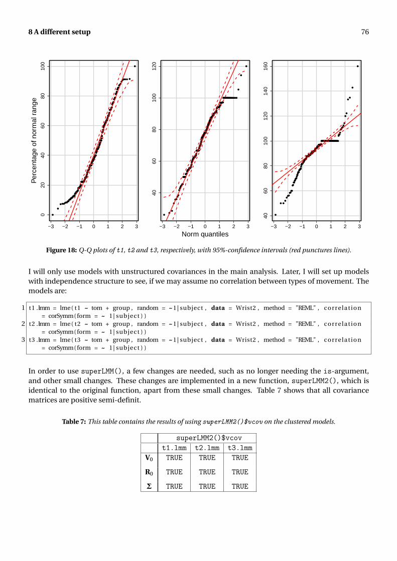
8 A different setup 76
−3 −2 −1 0 1 2 3
020
4060
8010
0
Per
cent
age
of n
orm
al r
ange
●
●
● ● ●● ●●
●●
●●●
●●●●
●●●●
●●
●●●●●●●
●●●●
●●●●●●●●●●●●●
●●●●●●●●●●●●●●●●●●●●
●●●●●●●
●●●
●●●
●●●●
●●●●●●
●●●
●●●●
●●●●●●●●●●●
●●●●●●●●●●●●
●●●●●●●●
●●●●●●●●●●●●
●●●●●●
●●●●●●●●●
●●●●●●
●●●●●●
●●●●●●●●
●
●●●
●●●●●
●●●
●●●●●●●●●●●●
●●●●●●●
●●
●
●●●●
●
●●
●●●●●
●●●
●●●
●●
●●
●●
●●
●
●
●●
●●
●
●
●● ● ● ●
●
−3 −2 −1 0 1 2 3
4060
8010
012
0
Norm quantiles
●
●
●
●
● ●
●
●
●
●
●●●●●
●●●●●●
●●●●
●●●●●●●
●●●●●●●●●●●
●
●●●
●●●●●●
●●●●●●●●●●●●
●●
●●●●●●●●●●●●●●●
●●●●●●●●●●●●●●●●●●
●
●●●●●●●●●●●
●●●●●●●●●●●●●●●●
●●
●●●●●●●●
●●●●
●●●●●●●●●
●●●●●●●●●●●●●●●●
●●●●●●●●●●●●●
●●●●●●●●●●●●
●●●
●
●●●●●●●●●●●
●●●●●
●●●●●●●●●●●
●●●●●●●●●●●●●●●●●●●● ● ● ●
●
●
●
−3 −2 −1 0 1 2 3
4060
8010
012
014
016
0
●
● ●
●
●
● ●
●●
●●
●●
●●
●●●●●
●
●●
●●●●
●●●●●●●
●
●●●●●●
●●●●●●
●●●●●●●●
●●●●
●●●●●●●●●●●●●●●●●●●●●●●●●
●●●●●●●●●●●●●●●●●●
●●●●●●●●●●●
●
●●●●●●●●●●●●●●●●●●●●
●●●●●●●●●●●●●●●●●●●●●●●
●●●●●●●●●●●●●●●●●●●●●●●●●●●●●●●●●●●●●●●●●●●●●●●●●●●●●●●●●●●●●●●●●●●●●●●●●●●●
●●●
●
●●
●●
●
●
●
●
●
●
●
●
Figure 18: Q-Q plots of t1, t2 and t3, respectively, with 95%-confidence intervals (red punctures lines).
I will only use models with unstructured covariances in the main analysis. Later, I will set up modelswith independence structure to see, if we may assume no correlation between types of movement. Themodels are:
1 t1 .lmm = lme ( t1 ~ tom + group , random = ~ 1 | subject , data = Wrist2 , method = "REML" , correlat ion= corSymm( form = ~ 1 | subject ) )
2 t2 .lmm = lme ( t2 ~ tom + group , random = ~ 1 | subject , data = Wrist2 , method = "REML" , correlat ion= corSymm( form = ~ 1 | subject ) )
3 t3 .lmm = lme ( t3 ~ tom + group , random = ~ 1 | subject , data = Wrist2 , method = "REML" , correlat ion= corSymm( form = ~ 1 | subject ) )
In order to use superLMM(), a few changes are needed, such as no longer needing the is-argument,and other small changes. These changes are implemented in a new function, superLMM2(), which isidentical to the original function, apart from these small changes. Table 7 shows that all covariancematrices are positive semi-definit.
Table 7: This table contains the results of using superLMM2()$vcov on the clustered models.
superLMM2()$vcovt1.lmm t2.lmm t3.lmm
V0 TRUE TRUE TRUE
R0 TRUE TRUE TRUE
Σ TRUE TRUE TRUE

8 A different setup 77
Table 8 shows that group is irrelevant to the models.
Table 8: The row for $anova1 are the p-values for group. The row for $anova2 are the p-values from the comparisonof the model and the null-model. The rows for $intervals are the 95%-confidence intervals for βgr.2 and βgr.3.
superLMM2()$groupt1.lmm t2.lmm t3.lmm
$anova1 0.18362 0.16467 0.99949
$anova2 0.17245 0.15515 0.88540
$intervals βgr.2 ∈ [−0.94,12.91] βgr.2 ∈ [−7.69,6.17] βgr.2 ∈ [−5.85,4.59]βgr.3 ∈ [−1.83,12.15] βgr.3 ∈ [−1.55,12.44] βgr.3 ∈ [−4.61,5.93]
Table 9 shows that all model assumptions are satisfied apart from the intercepts and residuals of t3.lmmbeing Gaussian.
Table 9: For both ass=1 (the intercepts) and ass=2 (the residuals), there are three rows. The first row are the p-valuesfrom the Bartlett test. The second row are the p-values from the Levene’s test, and the third row are the p-values fromthe Shapiro-Wilk test.
superLMM2(ass = c(1, 2))t1.lmm t2.lmm t3.lmm
ass = 1 0.29629 0.26388 0.773270.14325 0.15739 0.546480.97867 0.17024 0.00057
ass = 2 0.35055 0.60650 0.000000.99783 0.99993 0.936710.52707 0.40914 0.00000
−3 −2 −1 0 1 2 3
−40
−20
020
40
Norm quantiles
Res
idua
ls
●
●●
●
● ●●●
●●●●●
●●●●●
●●●●●
●●●●●●●
●●●●●●●
●●●●●●●
●●●●●●●●●●●●●●●
●●●●●●●●●●●●●●●
●●●●●●●●●●●●
●●●●●●●●●●●●●●●
●●●●●●●●●●●●●●●●
●●●●●●●●●●●●●●●●
●●●●●●●●●●●●●●●●●●
●●●●●●●●●●●●●●●●●
●●●●●●●●●●●●●●●●●●●●
●●●●●●●●●●●●●●●●●●
●●●●●●●●●●●●●
●●●●●
●●●●●●●●
●●●●
●●
●●
●●
●●
●
●
●
●
●
Residuals
Den
sity
−40 −20 0 20 40
0.00
0.02
0.04
0.06
Figure 19: Q-Q plot and histogram with density curve of the residuals of t3.lmm.

8 A different setup 78
Once again, the Q-Q plot and histogram of the residuals, seem to disagree on the distribution (see Figure19). From the histogram, I would consider the residuals Gaussian, but not from the Q-Q plot. But, mostimportantly, there are no violations of the homoscedasticity assumptions. Likewise for the intercepts.
I have now confirmed that the clustered models give less problems wrt. satisfying model assumptions,than the longitudinal models. Table 8 shows that the conclusion about the relevance of the treatmentgroups have, as suspected, not changed. I will now confirm this using Kenward-Rogers approxima-tion. As before, I set up models using lmer(). I am allowed to use this function despite it only havingthe exchangeable structure implemented. Just like with the longitudinal models, I have also here, inaddition to t1.lmm, t2.lmm and t3.lmm, set up the equivalent "in”- and "ex”-models and tested withanova(), that there is no significant difference in either of the models no matter the covariance struc-ture. This time the correlation parameters seemed more fitting with the numerically largest correlationfor all the "un”-models being 0.253, and the numerically largest for all the "ex”-models being 0.0014.Thus with clustered LMMs, we have results from anova() and the estimated correlation parameters,that are much more in agreement with each other than they were for the longitudinal models. And wemay assume no correlation between different types of movement. Table 10 shows the p-values from us-ing both KRmodcomp() and anova() on the "ex”-models made with lmer(). These results confirm thatH main
0 cannot be rejected.
Table 10: The p-values from KRmodcomp() and anova()with the full "ex”-models of t1, t2 and t3, respectively, andtheir corresponding null-models as input.
t1 t2 t3KRmodcomp() 0.16719 0.20460 0.92591
anova() 0.15634 0.19278 0.92324
8.2 Clustered GEE models
In Figure 18, we saw that the assumption of t3 being Gaussian may not be correct. Therefore, in thissection, I show the results from modelling t1, t2 and t3 with GEE models releaving me from makingany assumptions about the distribution of the response variables.
As in Section 8.1, I will only set up models with unstructured covariances in the main analysis, and Iwill use models with independence structure to see if we may assume no correlation between types ofmovement. The models are:
1 t1 . gee = geeglm ( t1 ~ tom + group , id = subject , data = Wrist2 , c o r s t r = " unstructured " , family =gaussian ( link = " i d e n t i t y " ) )
2 t2 . gee = geeglm ( t2 ~ tom + group , id = subject , data = Wrist2 , c o r s t r = " unstructured " , family =gaussian ( link = " i d e n t i t y " ) )
3 t3 . gee = geeglm ( t3 ~ tom + group , id = subject , data = Wrist2 , c o r s t r = " unstructured " , family =gaussian ( link = " i d e n t i t y " ) )
After replacing Wrist$group with Wrist2$group in superGEE(), giving me the almost identical func-tion superGEE2(), I can now analyse the models.
Table 11 shows that the residuals are homoscedastic and almost all are Gaussian. Just like for the clus-tered LMM for t3, the residuals of t3.gee are not Gaussian according to the Shapiro-Wilk test, and once

8 A different setup 79
again, the Q-Q plot and histogram seem to disagree with each other. These plots are not shown here,but they are very similar to Figure 19.
Table 11: The rows for test="homo" are the p-values of the Bartlett and Levene’s test, respectively, and the row fortest="norm" are the p-values of the Shapiro-Wilk test.
superGEE2(test = c("homo", "norm"))t1.gee t2.gee t3.gee
test = "homo" 0.35055 0.60650 0.000000.99783 0.99993 0.93671
test = "norm" 0.10500 0.24098 0.00000
Next, I will test if there is any difference between t1.gee, t2.gee and t3.gee and their corresponding"in”-models. Like in Section 7.4, I letδ denote the differences in the model based and empirical standarderrors. I have gathered the δ’s in matrices for t1, t2 and t3 shown below:
1 > modcomp. delta . t12 ( Intercept ) tomef tomur group2 group33 un 0.05496 0.15883 0.14182 0.12770 −0.368164 in 0.42541 −0.57795 −0.43274 1.06641 0.5682656 > modcomp. delta . t27 ( Intercept ) tomef tomur group2 group38 un −0.33969 −0.34815 −0.09747 0.05030 −0.519699 in 0.15816 −0.93454 −0.68378 1.32349 0.74645
1011 > modcomp. delta . t312 ( Intercept ) tomef tomur group2 group313 un −0.42868 −0.39995 −0.03886 −0.14085 −0.0323114 in −0.23999 −0.58775 −0.13083 0.30161 0.49650
We see that the δ’s for the "un”-models tend to be smaller than those of the "in”-models, indicating thatthere is correlation between the different types of movement. The sizes of a (see below) seems muchmore fitting for these model, than they were for the longitudinal GEE-models in Chapter 7.
1 > superGEE2 ( t1 . gee ) $ass . param2 alpha . 1 : 2 alpha . 1 : 3 alpha . 2 : 33 0.515 0.418 0.44245 > superGEE2 ( t2 . gee ) $ass . param6 alpha . 1 : 2 alpha . 1 : 3 alpha . 2 : 37 0.429 0.429 0.85089 > superGEE2 ( t3 . gee ) $ass . param
10 alpha . 1 : 2 alpha . 1 : 3 alpha . 2 : 311 0.168 0.084 0.371
Wtih clustered GEE models, we now have that the results from the δ’s and the a’s that are in much moreagreement with each other, than they were for the longitudinal models.
Finally, Table 12 shows group is irreleant to the models.

8 A different setup 80
Table 12: The row for $anova1 are the p-values for group. The row for $anova2 are the p-values from the compar-ison of the model and the null-model. The rows for $esticon are the 95%-confidence intervals for βgr.2 and βgr.3,and the p-values for these coefficients.
superGEE2()$groupt1.gee t2.gee t3.gee
$anova1 0.12889 0.10514 0.88910
$anova2 0.12889 0.10514 0.88910
$esticon βgr.2 ∈ [−0.70,12.88], 0.07862 βgr.2 ∈ [−7.25,6.44], 0.90737 βgr.2 ∈ [−4.96,4.36], 0.90040βgr.3 ∈ [−0.98,10.77], 0.10261 βgr.3 ∈ [−0.47,11.10], 0.07198 βgr.3 ∈ [−4.06,5.78], 0.73099
8.3 Conclusion
No matter if we use longitudinal or clustered models, whether we use ANOVA, MANOVA, LMMs or GEEmodels, there are no tests that indicate, Ibuprofen should have any significant beneficial effect on therecovery of wrist functions, and thus I conclude, that H main
0 cannot be rejected.

9 | Discussion
In this chapter, I present points for discussion. The points are presented in chronological order accord-ing to the sections in the report, where they appear, and are therefore not given in order of importance.
Subsection 4.2.2: Algorithm 4.2
Despite vigorous searching, I have not been able to find any sources either confirming or disprovingthat Algorithm 4.2 always converges, and that different choices for initial β could result in different finalβ’s. The source, [8], from which I have based this algorithm, mentions nothing about the subject. Fromhaving a look at the source code for lme(), I cannot tell for sure if the function is based on Algorithm4.2, but I must assume it is based on a similar algorithm. Hence, my questions about Algorithm 4.2may be answered through looking at the source code for lme(). In the source code, I looked to see if abreak is implemented in case convergence has not been reached within, say, 5000 iterations, meaningthat convergence is probably not going to happen. I found nothing of the sort. However, the argumentMaxIter in lme() is used for allowing for more iterations in order to reach convergence. There is noupper limit to MaxIter (here, I am assuming an upper limit would mean, that if convergence has notbeen reach with this number of iterations, then convergence is not going to happen at all), which canmean one of two things: either no upper limit is needed as convergence will always happen for bigenough MaxIter or it is assumed that the user knows that if the function has not converged even with,say, MaxIter = 5000, then the user should take that as a sign, that the function will not converge. Wrt.the choice for initial β, I believe it is chosen as (XT X)−1XT y because it lowers the number of iterationsneeded to reach convergence, just like how the initial β is chosen in Algorithm 6.2.
Subsection 4.3.2: Forϕ=σ2, we can set V0 =σ2A
There is no (logical) explanation in [7] as to why V0 can be written as σ2A when there is no correlationbetween subjects and autocorrelation within subjects. As
V0 =σ2uJn×n ⊗R0 = σ2
uJn×n ⊗σ2A
only if σ2u = 0 would V0 reduce to σ2A, but σ2
u is not zero. In A.14, we see that σ2u does not vanish
when deriving V−10 . I have chosen to derive the estimating equations for σ2
u , σ2 and ρ in the case withautoregressive structure. I see that in [7], had I chosen a different structure, then σ2
u would not havebeen overlooked when deriving the estimating equation for σ2. So either σ2
u was somehow forgotten inderiving the estimating equation for σ2 or it was left out on purpose, and the explanation for this waseither neglected or thought of as being so obvious, that the authors decided not to include it.
Section 5.4: Model comparison
When comparing the "ar”-, "un”- and "in”-models, I found that only for ps was the "un”-model preferedover the other two. But if I looked at the correlation parameters for all the "un”-models, it would seemthe "un”-models for ur and ef probably also should have been prefered over the "in”-models becauseof the high correlations. But perhaps these correlation were not high at all. When testing whether βi
could be set equal to zero, I used the function intervals(), which gave an interval for βi . If zero wascontained in the interval, we may set βi = 0. It would have been nice with such a test for the correlationparameters, so that if, say, ρ1,2 < c, for some limit c, we may set ρ1,2 = 0.

9 Discussion 82
An upside to these slightly confusing results is, that it allows me to use Kenward-Rogers approximation.For the Kenward-Rogers approximation, I must use a function in R which only has the exchangeablestructure implemented. This is no problem, as there is no significant difference in any of my models nomatter the covariance structure.
Section 7.3: Identical residuals
With the GEE models, I get identical residuals for both the "ar”-, "un”- and "in”-models for ps, andlikewise for ur and ef. This is despite having different R0, a, β (not shown in the report), and so onin these models, and it does not stem from a coding error in superGEE(). Investigating this further, Ilooked at the residuals for the GEE models in Example 5 (the respitory-data) where I had an "in”- andan "un”-model. Here, I also got identical residuals. Therefore, I believe these odd identical residuals arenot odd at all.
Section 7.4: Large association parameters
The estimated association parameters were a lot bigger than I would have expected. When looking atδ for all three type of models for one type of movement (modcomp.delta.ps, for instance), δ tendedto either be a little smaller for the "ar”- and "un”-models or about the same as the "in”-model. Hence,I would expect a to be small (although not zero). I cannot say how small, I would have expected it tobe, but certainly not larger than 0.5. Or perhaps, these are very reasonable results. I am basing myconcern on the large a’s on the results from Example 5. In this example, there was a clear difference inthe "in”- and "un”-models when looking at their corresponding δ. All entries in δ for the "un”-modelwas smaller by about a factor 10 than the corresponding entries in δ for the "in”-model. This resultedin a ∈ [0.209,0.439]. In the models for my data, instead of needing all entries in δ for either the "ar”-or "un”-model to be smaller than those in δ for the "in”-model, perhaps the large a is a result of someentries inδ for either the "ar”- or "un”-model being more than a factor 10 smaller than the correspondingentry in δ for the "in”-model. So, despite some of the entries in the different δ’s being almost equal, thefact that other entries differ quite some, may be enough to say that the "in”-models are actually lessfitting, and thus justifying the large a’s.
Chapter 8: Longitudinal vs. clustered models
When using clustered models instead of longitudinal models, I got results from comparing the "in”-and "un”-models that were much more in agreement with the estimated correlations between types ofmovement. This leads me to think, that when testing for the relevance of the treatment groups, thebetter set of models for this task, may be the clustered models. One concern I have, though, is theproblems with linearity. In the longitudinal models, I just had to add a squared term of time to havelinearity. Although I did have linearity for some patients in the clustered setup, for some patients thiswas certainly not so.
Other issues
I believe it is possible that how well and fast a patient recover wrist functions can be related to whetherthe injured hand is their dominant hand or not. After surgery, if the hand is stiff and sore, you might justchoose not to use it if it is your non-dominant hand. Hence, the hand will stay stiff for a longer time,because it is not being used. If instead the injured hand is the dominant hand, you might just use itanyway despite it being stiff and sore simply because it is your instinct. Hence, the wrist will get more"exercise” and will loosen up faster. It is interesting what the results would be, had I been able to includean indicator in my models of whether the injured hand was the dominant one or not.

Appendix A
This appendix contains calculations and results used in the report.
A. 1 The within-group variance, s2w , is an unbiased estimator of the common variance,σ2, if we have
that E[s2
w
]=σ2:
E[s2
w
]= 1
g
g∑i=1
E[s2
i
] (2.1)= 1
g
g∑i=1
1
n −1E
[n∑
j=1
(Yi j − Yi ·
)2
]
= 1
g (n −1)
g∑i=1
E
[n∑
j=1
(Y 2
i j + Y 2i · −2Yi j Yi ·
)]
= 1
g (n −1)
g∑i=1
E
[n∑
j=1Y 2
i j +nY 2i · −2Yi ·
n∑j=1
Yi j
]
= 1
g (n −1)
g∑i=1
E
[n∑
j=1Y 2
i j +nY 2i · −2Y 2
i ·
]= 1
g (n −1)
g∑i=1
E
[n∑
j=1Y 2
i j −nY 2i ·
]
= 1
g (n −1)
g∑i=1
(n∑
j=1E
[Y 2
i j
]−nE
[Y 2
i ·])
= 1
g (n −1)
g∑i=1
(n∑
j=1
(Var
[Yi j
]+E[Yi j
]2)−n
(Var
[Yi ·
]+E[Yi ·
]2))
= 1
g (n −1)
g∑i=1
(n∑
j=1
(σ2 +µ2
i
)−n
(σ2
n+µ2
i
))= 1
g (n −1)
g∑i=1
(nσ2 +nµ2
i −σ2 −nµ2i
)= 1
g (n −1)gσ2(n −1) = 1
g
g∑i=1
σ2 =σ2.
The between-group variance, s2b , is only an unbiased estimator of σ2 if µi =µ, ∀i :
E[s2
b
]= n
g −1E
[g∑
i=1
(Yi ·− Y··
)2
]= n
g −1
g∑i=1
(Var
[Yi ·
]+E[Yi ·
]−Var[Y··
]−E[Y··
])
= n
g −1
g∑i=1
(σ2
n+µ− 1
g 2gσ2
n− 1
ggµ
)= n
g −1
g∑i=1
σ2(
1
n− 1
nk
)
= n
g −1gσ2
(g −1
nk
)= σ2.
To get from the 1st to the 2nd equality, I used the approach from E[s2
w
]when going from the 2nd to
8th equality. Clearly, if µi 6=µ for some i , then E[s2
b
] 6=σ2.

84
A. 2 The total sum of squares and cross product matrix, T, can be written as a sum of
E =g∑
i=1
ni∑j=1
(yi j − yi ·)(yi j − yi ·)T
and
H =g∑
i=1ni (yi ·− y··)(yi ·− y··)
T :
T =g∑
i=1
ni∑j=1
(yi j − y··)(yi j − y··)T =
g∑i=1
ni∑j=1
((yi j − yi ·)+ (yi ·− y··)
)((yi j − yi ·)+ (yi ·− y··)
)T
=g∑
i=1
ni∑j=1
((yi j − yi ·)(yi j − yi ·)
T +2(yi j − yi ·)(yi ·− y··)T + (yi ·− y··)(yi ·− y··)
T)
=g∑
i=1
ni∑j=1
(yi j − yi ·)(yi j − yi ·)T +
g∑i=1
ni (yi ·− y··)(yi ·− y··)T +2
g∑i=1
ni∑j=1
(yi j − yi ·)(yi ·− y··)T
=g∑
i=1
ni∑j=1
(yi j − yi ·)(yi j − yi ·)T +
g∑i=1
ni (yi ·− y··)(yi ·− y··)T +2
g∑i=1
ni∑j=1
(yi j yT
i ·−yi j yT·· − yi ·y
Ti ·+ yi ·y
T··)
=g∑
i=1
ni∑j=1
(yi j − yi ·)(yi j − yi ·)T +
g∑i=1
ni (yi ·− y··)(yi ·− y··)T +2
g∑i=1
ni∑j=1
(yi j yT
i ·−yi j yT··)
−2g∑
i=1
(ni yi ·y
Ti ·+ni yi ·y
T··)
=g∑
i=1
ni∑j=1
(yi j − yi ·)(yi j − yi ·)T +
g∑i=1
ni (yi ·− y··)(yi ·− y··)T +2
g∑i=1
ni∑j=1
(yi j yT
i ·−yi j yT··)
−2g∑
i=1
(ni∑
j=1yi j yT
i ·+ni∑
j=1yi j yT
··
)
=g∑
i=1
ni∑j=1
(yi j − yi ·)(yi j − yi ·)T +
g∑i=1
ni (yi ·− y··)(yi ·− y··)T = E+H.
A. 3 Let λ be an eigenvalue of HE−1 = A with v as the corresponding eigenvector. Then Av = λv. LetB = A+ Ip×p . Then
Bv = (A+ Ip×p
)v = Av+ Ip×p v = λv+v = (λ+1)v.
This means that λ+1 is an eigenvalue of B. In Appendix B (see B.4), it is explained that the deter-minant of a matrix equals the product of the eigenvalues. Using this and the fact that |Ip×p | = 1, we

85
get
ΛW = |E||H+E| = |E||E−1|
|H+E||E−1| = |Ip×p ||A+ Ip×p |
= |A+ Ip×p |−1 = |B|−1 =p∏
i=1
1
1+λi.
Let C = A(A+ Ip×p )−1 = AB−1. Then
Cv = AB−1v = A(λ+1)−1v = 1
λ+1Av = λ
λ+1v.
This means that λλ+1 is an eigenvalue of C. In Appendix B (B.4), it is explained that the trace of a matrix
equals the sum of the eigenvalues. Using this and the trace is invariant under cyclic permutations,we get
ΛP = tr{
H(H+E)−1} = tr{
H(H+E)−1EE−1}= tr
{E−1H(H+E)−1 (
E−1)−1}
= tr{
A(HE−1 +EE−1)−1}= tr
{A(A+ Ip×p )−1} = tr {C} =
p∑i=1
λi
1+λi.
A. 4 Let Var[Ui ] =σ2u , ∀i , and Var
[εi j
]=σ2, ∀ j , and remember that ui and εi j are idependent, andthe εi j s are mutually independent. Observations within groups are correlated:
Corr[Yi j ,Yi l
]= Cov[Yi j ,Yi l
]√Var
[Yi j
]Var[Yi l ]
=12
(Var
[Yi j +Yi l
]−Var[Yi j
]−Var[Yi l ])√
Var[Yi j
]Var[Yi l ]
=12
(Var
[Yi j +Yi l
]− (σ2
u +σ2)− (
σ2u +σ2
))√(σ2
u +σ2)(σ2
u +σ2) =
12 Var
[Yi j +Yi l
]− (σ2
u +σ2)
σ2u +σ2
=12 Var
[2µ+ (xi j +xi l )β+2Ui +εi j +εi l
]−σ2u −σ2
σ2u +σ2
= 2Var[Ui ]+ 12 Var
[εi j +εi l
]−σ2u −σ2
σ2u +σ2
=12σ
2 + 12σ
2 −σ2 +σ2u
σ2u +σ2
= σ2u
σ2u +σ2
.
In the 2nd equality, Var[X +Y ] = Var[X ]+Var[Y ]+2Cov[X ,Y ] is used to change the numerator.
As Cov[X ,Y ] = 0 when X and Y are independent, obviously Corr[Yi j ,Ykl
]= 0 when i 6= k, i.e. whenYi j and Ykl are observations from different groups.

86
A. 5 The score function wrt. β is
Sβ(β;y) = ∂
∂β`(β;y)
(4.10)= −1
2
∂
∂β(y−Xβ)T V−1(y−Xβ) = −1
2
∂
∂β
(yV−1y−2yT V−1Xβ+βT XT V−1Xβ
)= ∂
∂β
(yT V−1Xβ− 1
2βT XT V−1Xβ
)= (
yT V−1X)T − (
βT XT V−1X)T = XT V−1y−XT V−1Xβ.
MLE of β is then
Sβ(β;y) = 0 ⇔ XT V−1y−XT V−1Xβ= 0 ⇔ β= (XT V−1X
)−1XT V−1y.
A. 6 If we want to predict the random variable X as much as possible by a constant c, the best pre-dictor for X will be c = E[X ]:
E[(X − c)2]= E
[(X −E[X ]+E[X ]− c)2] = E
[(X −E[X ])2]+2(E[X ]− c)E[X −E[X ]]+ (E[X ]− c)2
= E[(X −E[X ])2]+ (E[X ]− c)2 = Var[X ]+ (E[X ]− c)2.
A. 7 In order to find u, we must solve Su(β,ϕ;u,y) = 0, where the score function is given as
∂
∂u`(β,ϕ,u;y) =−1
2
∂
∂u
(log(|R(ϕ)|)+ (y−Xβ−Zu)T R(ϕ)−1(y−Xβ−Zu)+ log(|G(ϕ)|)+uT G(ϕ)−1u
)
=−1
2
∂
∂u
((y−Xβ−Zu)T R(ϕ)−1(y−Xβ−Zu)+uT G(ϕ)−1u
)=−1
2
∂
∂u
(yT R(ϕ)−1y+βT XT R(ϕ)−1Xβ+uT ZT R(ϕ)−1Zu−2yT R(ϕ)−1Xβ
−2yT R(ϕ)−1Zu−2βT XT R(ϕ)−1Zu+uT G(ϕ)−1u)
=−1
2
∂
∂u
(uT ZT R(ϕ)−1Zu−2yT R(ϕ)−1Zu+2βT XT R(ϕ)−1Zu+uT G(ϕ)−1u
)=−(
uT ZT R(ϕ)−1Z)T + (
yT R(ϕ)−1Z)T − (
βT XT R(ϕ)−1Z)T −G(ϕ)−1u
= ZT R(ϕ)−1 (y−Xβ−Zu
)−G(ϕ)−1u.
A. 8 We have that U ∼ Nm (0,G) and ε∼ NN (0,R), and u and ε are independent. Thus
Var[Y] = Var[Xβ+ZU+ε] = ZVar[U]ZT +Var[ε] = ZGZT +R.

87
A. 9 In the following are the calculations showing that the restricted log-likelihood can be written as`p(ϕ)− 1
2 log(|XT V(ϕ)−1X|). Let
A(ϕ) = XT V(ϕ)−1X (1)
B(ϕ) = A(ϕ)−1XT V(ϕ)−1. (2)
The term inside exp(·) in L(β,ϕ;y) (Equation (4.9)) can be rewritten as
(y−Xβ)T V(ϕ)−1(y−Xβ) = yT V(ϕ)−1y+βT XT V(ϕ)−1Xβ−2yT V(ϕ)−1Xβ
= yT V(ϕ)−1y+βT A(ϕ)β−2yT V(ϕ)−1Xβ
= yT V(ϕ)−1y+βT A(ϕ)β−2yT V(ϕ)−1Xβ+yT V(ϕ)−1XA(ϕ)−1XT V(ϕ)−1y
−yT V(ϕ)−1XA(ϕ)−1XT V(ϕ)−1y
= (βT −yT V(ϕ)−1XA(ϕ)−1)(A(ϕ)β−XT V(ϕ)−1y
)+yT V(ϕ)−1y
−yT V(ϕ)−1XA(ϕ)−1XT V(ϕ)−1y
= (βT −yT V(ϕ)−1XA(ϕ)−1)A(ϕ)
(β−A(ϕ)−1XT V(ϕ)−1y
)+yT V(ϕ)−1y
−yT V(ϕ)−1XA(ϕ)−1XT V(ϕ)−1y
= (β−A(ϕ)XT V(ϕ)−1y
)TA(ϕ)
(β−A(ϕ)−1XT V(ϕ)−1y
)+yT V(ϕ)−1y
−yT (A(ϕ)−1XT V(ϕ)−1)T
A(ϕ)(A(ϕ)−1XT V(ϕ)−1)y
= (β−B(ϕ)y
)T A(ϕ)(β−B(ϕ)y
)+yT V(ϕ)−1y−yT B(ϕ)T A(ϕ)B(ϕ)y. (3)
Notice, that β(ϕ) (Equation (4.13)) can be expressed as
β(ϕ)(1)= A(ϕ)−1XT V(ϕ)−1y
(2)= B(ϕ)y (4)
and so, the last two terms in Equation (3) can be written as
yT V(ϕ)−1y−yT B(ϕ)T A(ϕ)B(ϕ)y = yT V(ϕ)−1y+yT B(ϕ)T A(ϕ)B(ϕ)y−2yT B(ϕ)T A(ϕ)B(ϕ)y(4)= yT V(ϕ)−1y+ β(ϕ)T A(ϕ)β(ϕ)−2yT B(ϕ)T A(ϕ)β(ϕ)(2)= yT V(ϕ)−1y+ β(ϕ)T A(ϕ)β(ϕ)−2yT V(ϕ)−1XA(ϕ)−1A(ϕ)β(ϕ)(1)= yT V(ϕ)−1y+ β(ϕ)T XT V(ϕ)−1Xβ(ϕ)−2yT V(ϕ)−1Xβ(ϕ)
= (y−Xβ(ϕ))T V(ϕ)−1(y−Xβ(ϕ)). (5)
Using Equations (3) and (5), the term inside exp(·) is then
(y−Xβ)T V(ϕ)−1(y−Xβ) = (β−B(ϕ)y
)T A(ϕ)(β−B(ϕ)y
)+ (y−Xβ(ϕ))T V(ϕ)−1(y−Xβ(ϕ)). (6)

88
Thus we get∫L(β,ϕ;y) dβ
(4.9)=∫ (
1p
2πN|V(ϕ)|− 1
2 exp
(−1
2(y−Xβ)T V(ϕ)−1(y−Xβ)
))dβ
(6)=∫
1p
2πN|V(ϕ)|− 1
2
·exp
(−1
2
((β−B(ϕ)y
)T A(ϕ)(β−B(ϕ)y
)+ (y−Xβ(ϕ))T V(ϕ)−1(y−Xβ(ϕ))))
dβ
= 1p
2πN|V(ϕ)|− 1
2 exp
(−1
2(y−Xβ(ϕ))T V(ϕ)−1(y−Xβ(ϕ))
)·∫
exp
(−1
2
(β−B(ϕ)y
)T A(ϕ)(β−B(ϕ)y
))dβ
= 1p
2πN|V(ϕ)|− 1
2 exp
(−1
2(y−Xβ(ϕ))T V(ϕ)−1(y−Xβ(ϕ))
)·p2π
N |A(ϕ)|− 12
∫1
p2π
N|A(ϕ)| 1
2 exp
(−1
2
(β−B(ϕ)y
)T A(ϕ)(β−B(ϕ)y
))dβ
= 1p
2πN|V(ϕ)|− 1
2 exp
(−1
2(y−Xβ(ϕ))T V(ϕ)−1(y−Xβ(ϕ))
)·p2π
N |A(ϕ)|− 12 . (7)
The last equation deserves a short explanation: In the second to last equation, I multiplied by 1,so that the term in the integral became a likelihood function. In fact, the term in the integral hasthe form of a multivariate normal density with β as the variable. Integrating the density wrt. β is ofcourse just 1, giving the last equation.
Letting the squared roots cancel each other out, the restricted log-likelihood thus becomes
`R(ϕ)(4.15),(7)≡ −1
2log
(|V(ϕ)|)− 1
2(y−Xβ(ϕ))T V(ϕ)−1(y−Xβ(ϕ))− 1
2log
(|A(ϕ)|)(4.14)= `p(ϕ)− 1
2log
(|A(ϕ)|) (1)= `p(ϕ)− 1
2log
(|XT V(ϕ)−1X|) .
A. 10 The BLUP of u, when G =σ2uIm×m , Z = Im×m ⊗1T
n and V = Im×m ⊗ (σ2
uJn×n +R0):
u(4.12)= GZT V−1(y−Xβ)
(4.20),(4.21)= σ2uIm×m(Im×m ⊗1T
n )(Im×m ⊗ (
σ2uJn×n +R0
))−1(y−Xβ)
=σ2u(Im×m ⊗1)(Im×m ⊗1T
n )(Im×m ⊗ (
σ2uJn×n +R0
)−1)
(y−Xβ)
=σ2u
(Im×m ⊗1T
n
(σ2
uJn×n +R0)−1
)(y−Xβ) = σ2
u
(Im×m ⊗1T
n1
σ2u
(Jn×n + 1
σ2u
R0
)−1)(y−Xβ)
=(
Im×m ⊗1Tn
(1n1T
n + 1
σ2u
R0
)−1)(y−Xβ) =
(Im×m ⊗1T
n R−10
(1T
n R−10 1n + 1
σ2u
)−1)(y−Xβ)
= 1
r0 + 1σ2
u
(Im×m ⊗1T
n R−10
)(y−Xβ),
remembering that r0 = 1Tn R−1
0 1n .

89
A. 11 The estimate of β is independent ofϕ:
β= (XT V−1X)−1XT V−1y
= ((1m ⊗ In×n)T (Im×m ⊗V0)−1(1m ⊗ In×n)
)−1(1m ⊗ In×n)T (Im×m ⊗V0)−1y
= ((1T
m ⊗ In×n)(Im×m ⊗V−10 )(1m ⊗ In×n)
)−1(1T
m ⊗ In×n)(Im×m ⊗V−10 )y
= (1T
mIm×m1m ⊗ In×nV−10 In×n
)−1(1T
mIm×m ⊗ In×nV−10 )y
= (mV−1
0
)−1(1T
m ⊗V−10 )y = 1
m(1⊗V0)(1T
m ⊗V−10 )y = 1
m(1T
m ⊗ In×n)y
= 1
m
[In×n In×n · · · In×n
][y1 y2 · · · ym
]T
= 1
m
1 0 · · · 0 · · · 1 0 · · · 00 1 · · · 0 · · · 0 1 · · · 0...
.... . .
... · · · ......
. . ....
0 0 · · · 1 · · · 0 0 · · · 1
[y11 · · · y1n · · · · · · ym1 · · · ymn
]T
= 1
m
∑m
i=1 yi 1...∑m
i=1 yi n
=
y·1...
y·n
.
A. 12 The expression of the term 1Tn R−1
0 (yi − β) for the autoregressive covariance structure:
1Tn R−1
0 (yi − β) = 1
σ2(1−ρ2)
1−ρ
(1−ρ)2
...(1−ρ)2
1−ρ
T yi 1 − y·1yi 2 − y·2
...yi ,n−1 − y·n−1
yi n − y·n
= 1
σ2(1−ρ2)
(1−ρ)2 +ρ(1−ρ)
(1−ρ)2
...(1−ρ)2
(1−ρ)2 +ρ(1−ρ)
T yi 1 − y·1yi 2 − y·2
...yi ,n−1 − y·n−1
yi n − y·n
= 1
σ2(1−ρ2)
((1−ρ)2
n∑j=1
(yi j − yi ·
)+ρ(1−ρ)(yi 1 − y·1 + yi n − y·n)
)
= 1−ρσ2(1−ρ2)
((1−ρ)n(yi ·− y··)+ρ(yi 1 − y·1 + yi n − y·n)
).

90
A. 13 The expression of ui for the autoregressive covariance structure:
ui(4.23)= 1
(1−ρ)(2+(n−2)(1−ρ))σ2(1−ρ2)
+ 1σ2
u
· 1−ρσ2(1−ρ2)
((1−ρ)n(yi ·− y··)+ρ(yi 1 − y·1 + yi n − y·n)
)= 1−ρ
(1−ρ)(2+ (n −2)(1−ρ))+ σ2(1−ρ2)σ2
u
((1−ρ)n(yi ·− y··)+ρ(yi 1 − y·1 + yi n − y·n)
)
=(1−ρ)
σ2u
1−ρ((1−ρ)(2+ (n −2)(1−ρ))+ σ2(1−ρ2)
σ2u
)σ2
u1−ρ
((1−ρ)n(yi ·− y··)+ρ(yi 1 − y·1 + yi n − y·n)
)
= σ2u
σ2u(2+ (n −2)(1−ρ))+ σ2(1−ρ2)
1−ρ
((1−ρ)n(yi ·− y··)+ρ(yi 1 − y·1 + yi n − y·n)
)
=σ2
u
((1−ρ)n(yi ·− y··)+ρ(yi 1 − y·1 + yi n − y·n)
)σ2(1+ρ)+σ2
u(n −ρ(n −2)).
A. 14 We have, that V0 =σ2uJn×n +R0, and we must find V−1
0 :
V0 =σ2uJn×n +R0 ⇔ In×n =σ2
uJn×nV−10 +R0V−1
0 ⇔ R0V−10 = In×n −σ2
uJn×nV−10
⇔ V−10 = R−1
0 −σ2uR−1
0 Jn×nV−10 = R−1
0 −σ2uR−1
0 Jn×n(σ2
uJn×n +R0)−1
= R−10 −R−1
0 Jn×n
(Jn×n + 1
σ2u
R0
)−1
= R−10 −R−1
0 Jn×nR−10
(1T
n R−10 1n + 1
σ2u
)−1
= R−10 − 1
r0 + 1σ2
u
R−10 Jn×nR−1
0 = R−10 − 1
r0 + 1σ2
u
R−10 1n1T
n R−10 , (8)
remembering that r0 = 1Tn R−1
0 1n . Thus for ϕ=σ2u , LHS(ϕ) and RHS(ϕ) becomes
LHS(σ2u)
(4.25)= mtr
{V−1
0∂V0
∂σ2u
}= mtr
{V−1
0∂
∂σ2u
(σ2uJn×n +R0)
}= mtr
{V−1
0 Jn×n} = m1T
n V−10 1n
(8)= m1Tn
R−10 − 1
r0 + 1σ2
u
R−10 1n1T
n R−10
1n = m
1Tn R−1
0 1n − 1
r0 + 1σ2
u
1Tn R−1
0 1n1Tn R−1
0 1n
= m
r0 − 1
r0 + 1σ2
u
r 20
= mr0
1− r0
r0 + 1σ2
u
= mr0
r0 + 1σ2
u− r0
r0 + 1σ2
u
= mr0
r0σ2u +1
and
RHS(σ2u)
(4.25)= −(y−Xβ)T ∂V−1
∂σ2u
(y−Xβ) =−(y−Xβ)T ∂
∂σ2u
Im×m ⊗R−1
0 − 1
r0 + 1σ2
u
R−10 1n1T
n R−10
(y−Xβ)
= (y−Xβ)T ∂
∂σ2u
1
r0 + 1σ2
u
(Im×m ⊗R−1
0 1n1Tn R−1
0
)(y−Xβ)
= (y−Xβ)T ∂
∂σ2u
σ2u
r0σ2u +1
(Im×m ⊗R−1
0 1n1Tn R−1
0
)(y−Xβ)
= (y−Xβ)T 1
(r0σ2u +1)2
(Im×m ⊗R−1
0 1n1Tn R−1
0
)(y−Xβ).

91
A. 15 For ϕ=σ2, assuming that V0 =σ2A is correct, LHS(ϕ) and RHS(ϕ) becomes
LHS(σ2) = mtr
{V−1
0∂V0
∂σ2
}= mtr
{1
σ2A−1 ∂
∂σ2σ2A
}= mtr
{1
σ2A−1A
}= m
1
σ2tr{In×n} = 1
σ2mn
and with V−1 = Im×m ⊗ 1σ2 A−1, we get
RHS(σ2) =−(y−Xβ)T ∂V−1
∂σ2(y−Xβ)
= 1
σ4(y−Xβ)T (
Im×m ⊗A−1) (y−Xβ)
= 1
σ4
m∑i=1
(yi − β)T A−1(yi − β)
= 1
σ4
m∑i=1
yi 1 − y·1yi 2 − y·2
...yi n − y·n
T
A−1
yi 1 − y·1yi 2 − y·2
...yi n − y·n
= 1
σ4(1−ρ2)
m∑i=1
δi 1
δi 2
δi 3...
δi ,n−1
δi n
T
1 −ρ 0 . . . 0 0−ρ 1+ρ2 −ρ . . . 0 00 −ρ 1+ρ2 . . . 0 0...
......
. . ....
...0 0 0 . . . 1+ρ2 −ρ0 0 0 . . . −ρ 1
δi 1
δi 2
δi 3...
δi ,n−1
δi n
= 1
σ4(1−ρ2)
m∑i=1
δi 1
δi 2
δi 3...
δi ,n−1
δi n
T
δi 1 −ρδi 2
−ρδi 1 + (1+ρ2)δi 2 −ρδi 3
−ρδi 2 + (1+ρ2)δi 3 −ρδi 4...
−ρδi ,n−2 + (1+ρ2)δi ,n−1 −ρδi n
−ρδi ,n−1 +δi n
= 1
σ4(1−ρ2)
m∑i=1
(δi 1(δi 1 −ρδi 2)+δi 2(−ρδi 1 + (1+ρ2)δi 2 −ρδi 3)
+δi 3(−ρδi 2 + (1+ρ2)δi 3 −ρδi 4)+ . . .+δi ,n−1(−ρδi ,n−2 + (1+ρ2)δi ,n−1 −ρδi n)
+δi n(−ρδi ,n−1 +δi n))
= 1
σ4(1−ρ2)
m∑i=1
(δ2
i 1 +δ2i n −2ρ
n∑j=2
δi , j−1δi j + (1+ρ2)n−1∑j=2
δ2i j
)= 1
σ4(1−ρ2)
m∑i=1
((1+ρ2)
n∑j=1
δ2i j −ρ2(δ2
i 1 +δ2i n)−2ρ
n∑j=2
δi , j−1δi j
).

92
A. 16 For ϕ= ρ, LHS(ϕ) and RHS(ϕ) becomes
LHS(ρ) = mtr
{V−1
0∂V0
∂ρ
}= mtr
{1
σ2A−1 ∂
∂ρσ2A
}
= mtr
{A−1 ∂
∂ρA}
= − ρ
1−ρ22m(n −1).
Here, I skip the calculation of A−1 ∂∂ρA, as it is quite comprehensive, and relying on the result in [7].
And
RHS(ρ) =−(y−Xβ)T ∂V−1
∂ρ(y−Xβ)
=−(y−Xβ)T(
1
σ2Im×m ⊗ ∂
∂ρA−1
)(y−Xβ)
= 1
σ2
m∑i=1
δi 1
δi 2
δi 3...
δi ,n−1
δi n
T
∂
∂ρA−1
δi 1
δi 2
δi 3...
δi ,n−1
δi n
= 1
σ2(1−ρ2)2
m∑i=1
δi 1
δi 2
δi 3...
δi ,n−1
δi n
T
2ρ −(1+ρ2) 0 . . . 0 0−(1+ρ2) 4ρ −(1+ρ2) . . . 0 0
0 −(1+ρ2) 4ρ . . . 0 0...
......
. . ....
...0 0 0 . . . 4ρ −(1+ρ2)0 0 0 . . . −(1+ρ2) 2ρ
δi 1
δi 2
δi 3...
δi ,n−1
δi n
=− 1
σ2(1−ρ2)2
m∑i=1
(4ρ
n∑j=1
δ2i j −2ρ(δ2
i 1 +δ2i n)−2(1+ρ2)
n∑j=2
δi , j−1δi j
).
The last equation comes from the expression of RHS(σ2). The calculations in RHS(ρ) are the sameas in RHS(σ2), only − 1
σ4 A−1 is replaced by 1σ2
∂∂ρ
A−1.
A. 17 The estimate of µi is a weighted average between the overall mean, µ, and the group averageobservation, yi ·. We have, that
Var[Yi ·
]= Var
[1
n
n∑j=1
Yi j
]= Var
[1
n
n∑j=1
µi
]+Var
[1
n
n∑j=1
εi j
]= Var
[1
nnµi
]+ 1
n2
n∑j=1
Var[εi j
]
= Var[µi
]+ 1
n2nVar
[εi j
]=σ2u + σ2
n,

93
and
E[Yi ·
]= E
[1
n
n∑j=1
Yi j
]= E
[1
n
n∑j=1
µi
]+E
[1
n
n∑j=1
εi j
]
= E
[1
nnµi
]+ 1
n
n∑j=1
E[εi j
] = E[µi
] = µ.
This means that the best prediction of the group average mean is found by conditioning on what wealready know, i.e. yi ·:
µi = E[µi | Yi ·
] = E[µi
]+Cov[µi , Yi ·
] 1
Var[Yi ·
] (yi ·−E
[Yi ·
])=µ+ (
E[µi Yi ·
]−E[µi
]E
[Yi ·
]) 1
σ2u + σ2
n
(yi ·−µ
)
=µ+(
E
[µi
1
n
n∑j=1
(µi +εi j )
]−µ2
)1
σ2u + σ2
n
(yi ·−µ
)
=µ+(
E[µ2
i
]−E
[1
n
n∑j=1
µiεi j
]−µ2
)1
σ2u + σ2
n
(yi ·−µ
)
=µ+(σ2
u +µ2 − 1
n
n∑j=1
E[µi
]E
[εi j
]−µ2
)1
σ2u + σ2
n
(yi ·−µ
)
=µ+ σ2u
σ2u + σ2
n
(yi ·−µ
) =(
1− σ2u
σ2u + σ2
n
)µ+ σ2
u
σ2u + σ2
n
yi ·.
A. 18 We have, that Ui ∼ N(0,σ2
u
). The covariance between the total residuals at two timepoint is
just the variance of the random intercepts:
Cov[Yi j ,Yi k
]= Cov[Ui +εi j ,Ui +εi k
]= E
[(Ui +εi j )(Ui +εi k )
]−E[Ui +εi j
]E[Ui +εi k ]
= E[U 2
i
]+E[εi j εi k
]+E[Uiεi k ]+E[Uiεi k ]−0
=σ2u .

94
A. 19 The covariance of the total residual is
Cov[Yi j ,Yi k
]= Cov[Ui +xi j bi +εi j ,Ui +xi k bi +εi k
]= E
[(Ui +xi j bi +εi j )(Ui +xi k bi +εi k )
]−E[Ui +xi j bi +εi j
]E[Ui +xi k bi +εi k ]
= E[U 2
i
]+xi j xi k E[b2
i
]+E[εi j εi k
]+ (xi j +xi k )E[Ui bi ]+E[Ui (εi j +εi k )
]+xi j E[biεi k ]+xi k E
[biεi j
]−0
=σ2u +xi j xi kσ
2b + (xi j +xi k )E[Ui bi ]
=σ2u +xi j xi kσ
2b + (xi j +xi k )
(Cov[Ui ,bi ]+E[Ui ]E[bi ]
)=σ2
u +xi j xi kσ2b + (xi j +xi k )σub .
A. 20 When a random variable, Yi , has a distribution from the exponential family, the mean value ofYi can be expressed as b′(θi ). To show this, we use the fact that the mean of a random variable, X , isdefined as E[X ] = ∫
x f (x) d x:
d
dθi
∫f (yi ;θi ,φ) d yi =
∫d
dθif (yi ;θi ,φ, ) d yi
(6.1)=∫
h(yi ,φ
) d
dθiexp
(yiθi −b(θi )
φ
)d yi
=∫
h(yi ,φ
)exp
(yiθi −b(θi )
φ
)(yi −b′(θi )
φ
)d yi
= 1
φ
∫ (yi f (yi ;θi ,φ)−b′(θi ) f (yi ;θi ,φ)
)d yi (9)
= 1
φ
(∫yi f (yi ;θi ,φ) d yi −b′(θi )
∫f (yi ;θi ,φ) d yi
)(10)
= 1
φ
(E[Yi ]−b′(θi )
)= 0
mE[Yi ] = b′(θi ).
The variance of Yi can be expressed as φb′′(θi ). To show this, we use the fact that the variance of a

95
random variable, X , is defined as Var[X ] = E[(X −E[X ])2
]= E[
X 2]−E[X ]2:
d 2
dθ2i
∫f (yi ;θi ,φ) d yi =
∫d 2
dθ2i
f (yi ;θi ,φ) d yi
(10)= 1
φ
(∫yi
d
dθif (yi ;θi ,φ) d yi −
∫d
dθib′(θi ) f (yi ;θi ,φ) d yi
)(9)= 1
φ
[1
φi
∫yi
(yi f (yi ;θi ,φ)−b′(θi ) f (yi ;θi ,φ)
)d yi
−∫ (
b′′(θi ) f (yi ;θi ,φ)+b′(θi )d
dθif (yi ;θi ,φ)
)d yi
]
= 1
φ2
(E
[Y 2
i
]−b′(θi ))− 1
φb′′(θi )
∫f (yi ;θi ,φ) d yi
− 1
φb′(θ)
∫d
dθif (yi ;θi ,φ) d yi
= 1
φ2
(E
[Y 2
i
]−b′(θi ))− 1
φb′′(θi )− 1
φb′(θi )
(1
φ
(E[Yi ]−b′(θi )
))
= 1
φ2
(E
[Y 2
i
]−E[Yi ])− 1
φb′′(θi )− 1
φb′(θi )
(1
φ(E[Yi ]−E[Yi ])
)
= 1
φ2 (Var[Yi ])− 1
φb′′(θi )
= 0
mVar[Yi ] =φb′′(θi ).
A. 21 Remember, that µi = b′(θi ), θi = b′(µi )−1 and V (µi ) = b′′ (b′(µi )−1). Thus the score function is
∂`i
∂µi= ∂`i
∂θi× ∂θi
∂µi
(6.1)= yi −b′(θi )
φ×
(∂µi
∂θi
)−1
= yi −b′(θi )
φ×
(∂b′(θi )
∂θi
)−1
= yi −b′(θi )
φ× (
b′′(θi ))−1
= yi −b′(θi )
φ× 1
b′′(b′(µi )−1)
= yi −b′(θi )
φ× 1
V (µi ).

96
A. 22 The function qi satisfies the properties E[qi
]= 0 and Var[qi
]=−E[∂qi∂µi
], meaning it mimics a
proper score function:
E[qi
]= E[Yi ]−µi
φV (µi )= 0
Var[qi
]= Var[Yi −µi
]φ2V (µi )2
= φV (µi )
φ2V (µi )2= 1
φV (µi )
−E
[∂qi
∂µi
]=−E
[Yi
φ
∂
∂µi
1
V (µi )− 1
φ
∂
∂µi
µi
V (µi )
]=−E
[−Yi
φ
V ′(µi )
V (µi )2− 1
φ
V (µi )−µi V ′(µi )
V (µi )2
]
=−E
[−Yi V ′(µi )−V (µi )+µi V ′(µi )
φV (µi )2
]=−
(−E[Yi ]V ′(µi )−V (µi )+µi V ′(µi )
φV (µi )2
)
= V (µi )
φV (µi )2= 1
φV (µi ).
A. 23 The mean value of r j k is just the correlation ρ j k :
E[r j k
]= E[(Yi j −µi j )(Yi k −µi k )
]φ
√V (µi j )V (µi k )
= Cov[Yi j ,Yi k
]√φ2V (µi j )V (µi k )
= Cov[Yi j ,Yi k
]√Var
[Yi j
]Var[Yi k ]
= Corr[Yi j ,Yi k
]= ρ j k .

Appendix B
This appendix contains additional theory that may be helpful for the reader.
B. 1 (The anova-function in R) When giving anova() two inputs, the function performs a compar-ison of the models, which must be nested. The comparison is based on AIC (Akaike’s InformationCriterion). AIC is given as
AIC = 2p −2log(L),
where p is the number of parameters in the model and L is the maximum value of the likelihoodfunction for the model. When given an increasing input, log(·) is an increasing function. For a fixed p,AIC will decrease as log(L) increases. And AIC will be at its minimum when log(L) is at its maximum,i.e. when L = L. As the objective is always, that we want L maximized, the objective of the AIC isto have it minimized. When comparing two models with, say, AICmodel1 and AICmodel2, the bettermodel will be the one with the smallest AIC . But how big does the difference in AIC have to be for usto say that AICmodel1 6= AICmodel2? For this, anova() also provides a p-values. The hypothesis testedin anova() is
H anova10 : The AIC of the models are the same.
For a p-value below the level α, H anova10 is rejected.
When giving anova() just one input, the function tests whether the model terms are significant, i.e.whether the estimated coefficients are significant. The hypothesis is
H anova20 :β1, . . . ,βp are significant.
The test statistic is
F = N −k
k −1·
∑ki=1 ni (yi ·− y··)2∑k
i=1
∑nij=1(yi j − yi ·)2
,
where k is the number of samples, ni is the size of sample i , N = ∑ki=1 ni , yi j is the observation of
the j th subject in the i th sample, yi · is the sample mean for the i th sample, and y·· is the overallmean. The test statistic is approximately F -distributed with k −1 and N −k degrees of freedom, andH anova2
0 is rejected if F > F (α,k −1, N −k) for a chosen level α.
Based on https://en.wikipedia.org/wiki/F-test.
B. 2 (F -test) An F -test is not one particular test, but rather any statistical test in which the teststatistic follows an F -distribution under H0. Examples of F -tests are given in B.4, B.6 and B.7.The F -test is sensitive to non-normality. When doing analysis of variance, the assumption ofhomoscedasticity is more easily violated, when the normality assumption is violated.
Based on https://en.wikipedia.org/wiki/Mauchly%27s_sphericity_test.

98
B. 3 (Eigenvalues) An eigenvalue is a scalar, that satisfies Av = λv for a matrix A, where v is calledthe corresponding eigenvector.
Let λi for i = 1, . . . ,n be the eigenvalues (including multiplicity) of A ∈Rn×n . Then
tr{A} =n∑
i=1λi and |A| =
n∏i=1
λi .
Eigenvalues can also be thought of as roots as they are the solutions to the characteristic polynomial|A−λIn×n |.Based on https://en.wikipedia.org/wiki/Determinant#Relation_to_eigenvalues_and_trace.
B. 4 (Shapiro-Wilk test) The Shapiro-Wilk test tests the hypothesis
H shapiro0 : sample is from a normally distributed population.
The test statistic is
W =(∑n
i=1 ai y(i ))2∑n
i=1
(yi − y
)2 ,
where data is arranged in ascending order with y(i ) being the i th smallest observation in the sample,y is the sample mean and
a1
a2...
an
= mT V −1(mT V −1V −1m
) 12
with m = E[Yi ] iid.∼ N (0,1) and V being the covariance matrix of the y(i )s. A p-value lower than thechosen level αmeans H0 is rejected. The p-value is found in a table using the sample size, n, and thecalculated test statistic, W .
Based on https://en.m.wikipedia.org/wiki/Shapiro–Wilk_test.
B. 5 (Kruskal-Wallis) When the assumption of Gaussian samples fail, one can use the Kruskal-Wallistest as an alternative to the one-way ANOVA. This test makes no assumptions about the distributionof the samples. It tests the hypothesis
H kruskal0 : the medians of all the groups are equal.
The test works by first arranging all the values in all the samples by rank. Let ri j denote the rank ofthe observation yi j . The test statistic is
K = (N −1)
∑gi=1 ni (ri ·− r )2∑k
i=1
∑nij=1
(ri j − r
)2 ,
where ri · = ∑nij=1 ri j is the average rank for observations in group i , r = N+1
2 is the average of all theranks, N is the total number of observation and ni is the number of observations in group i . The

99
test statistic is approximately χ2-distributed with g −1 degrees of freedom, and H kruskal0 is rejected if
K >χ2g−1,α for a chosen level α.
Based on https://en.wikipedia.org/wiki/Kruskal–Wallis_one–way_analysis_of_variance.
B. 6 (Bartlett test) The Bartlett test tests the hypothesis
H bartlett0 : variances across samples are equal.
The test statistic is
χ2 =(N −k) log
(s2
p
)−∑k
i=1 (ni −1)log(s2
p
)1+ 1
3(k−1)
(∑ki=1
1ni−1 − 1
N−k
) ,
where k is the number of samples, ni is the size of sample i , N = ∑ki=1 ni , and s2
p = 1N−k
∑ki=1 s2
i with
s2i being the i th sample variance. The test statistic is approximately χ2-distributed with k−1 degrees
of freedom, and H0 is rejected if χ2 >χ2k−1,α for a chosen level α.
Based on https://en.wikipedia.org/wiki/Bartlett%27s_test.
B. 7 (Levene’s test) The Levene’s test tests the same hypothesis as the Bartlett test, but does so usingthe F -distribution. The test statistic is
F = N −k
k −1·
∑ki=1 ni (zi ·− z··)2∑k
i=1
∑nij=1(zi j − zi ·)2
,
where k is the number of samples, ni is the size of sample i , N = ∑ki=1 ni , zi j = |yi j − yi ·| with yi j
being the observation of the j th subject in the i th sample and yi · is the sample mean for the i thsample, zi · = 1
ni
∑nij=1 zi j and z·· = 1
N
∑ki=1
∑nij=1 zi j . The test statistic is approximately F -distributed
with k −1 and N −k degrees of freedom, and H levene0 is rejected if F > F (α,k −1, N −k) for a chosen
level α.
Based on https://en.m.wikipedia.org/wiki/Levene%27s_test.
B. 8 (Conditional multivariate distribution) For(X1
X2
)∼ Nn+m
([µ1µ2
],
[Σ1 Σ12
Σ21 Σ2
])we have that X1 | X2 = x2 ∼ Nn
(µ1 +Σ21Σ
−12 (x2 −µ2),Σ1 −Σ21Σ
−12 Σ12
).

100
B. 9 (Direct product) Below are all the rules for direct product used in this report.
Direct product: For A ∈Rn×m and B ∈Rs×t , the direct product is
A⊗B =
a11B a12B . . . a1mBa21B a22B . . . a2mB
......
. . ....
an1B an2B . . . a1nmB
∈Rns×mt .
Direct sum: For matrices A j ∈Rn j×m j , the direct sum is
J⊗j=1
A j = A1 ⊗A2 ⊗·· ·⊗AJ .
Sum: The sum of two direct sums for matrices A j ∈Rn j×m j and B j ∈Rn j×m j is(J⊗
j=1A j
)+
(J⊗
j=1B j
)=
J⊗j=1
(A j +B j ).
Product: The product of two direct sums for matrices A j ∈Rn j×m j and B j ∈Rm j×k j is(J⊗
j=1A j
)(J⊗
j=1B j
)=
J⊗j=1
(A j B j ).
Transpose: The transpose of the direct product of matrices A ∈Rn×m , B ∈Rk×l , and C ∈Rs×t is
(A⊗B⊗C)T = AT ⊗BT ⊗CT
Inverse: The inverse of the direct product of matrices A ∈Rn×m and B ∈Rs×t is
(A⊗B)−1 = A−1 ⊗B−1
Commutative law: For a constant c and a matrix A ∈Rn×m , we have
c ⊗A = A⊗ c = cA.
Distributive law: For matrices A ∈Rn×m , B ∈Rn×m , and C ∈Rs×t , we have
(A+B)⊗C = (A⊗C)+ (B⊗C)
C⊗ (A+B) = (C⊗A)+ (C⊗B).
Based on https://en.wikipedia.org/wiki/Kronecker_product.
B. 10 (Derivative of determinant) For a square matrix A dependent on t , we have
d
d t|A(t )| = |A(t )|tr
{A(t )−1 d
d tA(t )
}.
Based on https://en.wikipedia.org/wiki/Jacobi%27s_formula.

101
B. 11 (Likelihood ratio test) Let θ be the maximum likelihood estimate of the parameter θ ∈ Rp×1.We want to test the hypothesis
H LRT0 : θ = θ0,
where θ0 is a proposed value of θ. To test H LRT0 , we look at the ratio between the likelihood with the
proposed value, L(θ0), and the likelihood with the estimated value, L(θ), i.e. we look at L(θ0)/L(θ).If this ratio is very small, then the data with θ is more plausible than the data with θ0, which meansH LRT
0 is rejected. More precisely, the likelihood ratio test statistic is given by
−2LR =−2(`(θ0)−`(θ)
)and H LRT
0 is rejected if −2LR >χ2p,α for a chosen level α.
Based on https://en.m.wikipedia.org/wiki/Likelihood-ratio_test.
B. 12 (Wald test) Assume that θ is a consistent estimate of the parameter θ ∈Rp×1. Then
θ ∼ Np(θ, I (θ)−1) ,
assymptotically, where I (θ) is the information matrix. The standard error of θi is σi =√
Var[θ]
i i .The Wald statistic is
Wi =θi −θi ,0
σi,
where θi ,0 is the proposed value of θi . Under
H wald0 : θi = θi ,0
Wi will be approximately N (0,1)-distributed. It is not uncommon to write the statistic as
W 2i =
(θi −θi ,0
)2
σ2i
,
which under H wald0 is χ2-distributed with 1 degree of freedom. We reject H wald
0 if Wi > χ21,α for a
chosen level α.
Based on https://en.m.wikipedia.org/wiki/Wald_test.
mellemrummellemrummellemrummellemrummellemrummellemrummellemrummellemrummellemrummellemrum

102
mellemrum
mellemrummellemrummellemrummellemrummellemrum

References
[1] Author(s): P. Olofsson & M. AnderssonTitle: Probability, Statistics, and Stochastic Processes, 2nd Ed., chapter 7Publisher: WileyYear: 2012
[2] Author(s): D. Hedeker & R. D. GibbonsTitle: Longitudinal Data Analysis, chapters 2, 4, 6 and 8Publisher: WileyYear: 2006
[3] Author(s): A. Field, University of Sussex,Title: A Bluffer’s Guide to ... Sphericity,Year: 2017
[4] Author(s): The Pennsylvania State University,www:.https://onlinecourses.science.psu.edu/stat505/node/159, chapters 8.2 and 8.3Year: 2018
[5] Author(s): G. Carey, University of Colorado, Boulder,www:.http://ibgwww.colorado.edu/∼carey/p7291dir/handouts/manova1.pdfYear: 1998
[6] Author(s): E. DemidenkoTitle: Mixed Models: Theory and Applications, chapters 1 and 2Publisher: WileyYear: 2004
[7] Author(s): C. E. McCullogh & S. R. SearleTitle: Generalized, Linear, and Mixed Models, chapters 5 and 7Publisher: WileyYear: 2001
[8] Author(s): H. Madsen & P. ThyregodTitle: Introduction to General and Generalized Linear Models, chapter 5Publisher: CRC PressYear: 2011
[9] Author(s): C. Czado (Technische Universität München)www:.http://www2.stat.duke.edu/∼sayan/Sta613/2017/lec/LMM.pdfYear: 2017
[10] Author(s): B. S. Everitt & T. HothornTitle: A Handbook of Statistical Analysis Using R, chapter 12Publisher: CRC PressYear: 2010

104
[11] Author(s): U. Halekoh & S. HøjsgaardTitle: A Kenward-Roger Approximation and Parametric Bootstrap Methods for Tests in Linear MixedModels – the R Package pbkrtest,Publisher: American Statistical AssociationYear: 2014
[12] Author(s): M. A. Islam & R. I. ChowdhuryTitle: Analysis of Repeated Measures Data, chapters 11 and 12Publisher: SpringerYear: 2017
[13] Author(s): G. Fitzmaurice, M. Davidian, G. Verbeke & G. MolenberghsTitle: Longitudinal Data Analysis, chapter 3Publisher: CRC PressYear: 2009