State Standard 9-02 July 2002

ARIZONA DEPARTMENT OF WATER RESOURCESDAM SAFETY SECTION

State Standard

for

Floodplain Hydraulic Modeling

Under the authority outlined in ARS 48-3605(A) the Director of the ArizonaDepartment of Water Resources establishes the following standard forFloodplain Hydraulic Modeling in Arizona.

The guidelines outlined in State Standard Attachment 9-02 entitled "FloodplainHydraulic Modeling," or an alternative procedure reviewed and accepted by theDirector, will be used in modeling floodplains for fulfilling the requirements ofFlood Insurance Studies and local community and county flood damageprevention ordinances.

Floodplain hydraulic modeling standards will apply to all watercoursesidentified by the Federal Emergency Management Agency as part of theNational Flood Insurance Program, all watercourses that have been identifiedby local floodplain administrators as having significant potential flood hazardsand all watercourses with drainage areas more than 1/4 square mile or a100-year discharge estimate of more than 500 cubic feet per second.Application of these guidelines will not be necessary if the local community orcounty has in effect a drainage, grading or stormwater ordinance that, in theopinion of the Department, results in the same or greater level of floodprotection as application of these guidelines.

This requirement is effective July 30, 2002.

Copies of this State Standard and State Standard Attachment can be obtainedby contacting the Department's Dam Safety Section at (602) 417-2445.

State Standard 9-02 July 2002

State Standard Attachment July 2002SSA9-02

ARIZONA DEPARTMENT OF WATER RESOURCESDAM SAFETY SECTION

Floodplain Hydraulic Modeling

500 North Third StreetPhoenix, Arizona 85004

(602) 417-2445

State Standard Attachment July 2002SSA9-02

DISCLAIMER OF LIABILITY

The Arizona Department of Water Resources is not responsible for the application ofthe methods outlined in this publication and accepts no liability for their use. Soundengineering judgment is recommended in all cases.

The Arizona Department of Water Resources reserves the right to modify, update, orotherwise revise this document. Questions regarding information contained in thisdocument and/or floodplain management should be directed to the local floodplainadministrator or the office below:

Dam Safety SectionArizona Department of Water Resources500 North Third StreetPhoenix, Arizona 85004

Phone: 602-417-2445FAX: 602-417-2423

SSA9-02 July 2002i

TABLE OF CONTENTS

1. INTRODUCTION........................................................................................11.1 PURPOSE AND BACKGROUND .......................................................................................... 11.2 GENERAL ....................................................................................................................... 11.3 OVERVIEW ..................................................................................................................... 11.4 RELATED STATE STANDARDS ......................................................................................... 2

2. ONE-DIMENSIONAL HYDRAULIC MODELS ......................................32.1 GENERAL ....................................................................................................................... 32.2 DEFINITION .................................................................................................................... 32.3 MODEL SELECTION CONSIDERATIONS ............................................................................. 3

2.3.1 Steady versus Unsteady Flow................................................................................... 32.3.2 Abilities and Limitations of Common Models........................................................... 42.3.3 Backwater (Multiple Cross Section) versus Single Cross Section Models................. 52.3.4 Acceptance and Availability of Models .................................................................... 5

2.4 1-D MODEL LIMITATIONS............................................................................................... 52.5 DATA REQUIREMENTS AND COLLECTION ........................................................................ 6

3. CHANNEL GEOMETRY............................................................................73.1 GENERAL ....................................................................................................................... 73.2 MAPPING REQUIREMENTS FOR HYDRAULIC MODELING AND FLOODPLAIN DELINEATION.. 7

3.2.1 Flood Insurance Studies .......................................................................................... 73.3 CROSS SECTIONS ............................................................................................................ 8

3.3.1 Location, Alignment, Configuration, and Spacing.................................................... 83.3.2 Addition of Cross Sections When Analyzing Proposed Conditions ......................... 113.3.3 Subdivision and Channel Bank Locations .............................................................. 113.3.4 Reach Lengths ....................................................................................................... 113.3.5 Encroachments, Blocked and Ineffective Flow Areas ............................................. 12

3.3.5.1 Levees ...........................................................................................................123.3.5.2 Structures.......................................................................................................12

3.3.6 Interpolation of Cross Sections .............................................................................. 143.3.7 Cross Section Location at Tributaries.................................................................... 14

4. INFLOWS AND OUTFLOWS..................................................................164.1 LOCAL INFLOWS AND OUTFLOWS.................................................................................. 164.2 TRIBUTARIES, DISTRIBUTARIES, AND BREAKOUTS ........................................................ 16

5. SPECIAL TOPICS.....................................................................................195.1 MODELING OF HYDRAULIC STRUCTURES ...................................................................... 19

5.1.1 Bridges .................................................................................................................. 19

SSA9-02 July 2002ii

5.1.1.1 General Guidelines.........................................................................................195.1.1.2 Specific Guidelines ........................................................................................20

5.1.1.2.1 Locating Bridge Cross Sections..................................................................205.1.1.2.2 Modeling Low Flow...................................................................................225.1.1.2.3 Modeling High Flow..................................................................................225.1.1.2.4 Perched Bridges .........................................................................................235.1.1.2.5 Low Water Bridges ....................................................................................235.1.1.2.6 Skewed Bridges .........................................................................................235.1.1.2.7 Parallel Bridges..........................................................................................235.1.1.2.8 Multiple Bridge Openings ..........................................................................245.1.1.2.9 Modeling Floating Debris on Piers .............................................................24

5.1.2 Culverts ................................................................................................................. 245.1.3 Weirs ..................................................................................................................... 24

5.2 STRUCTURES IN THE FLOODPLAIN ................................................................................. 255.3 SELECTION OF ROUGHNESS VALUES ............................................................................. 255.4 BENDS ......................................................................................................................... 275.5 MODELING SUPERCRITICAL AND MIXED FLOW.............................................................. 275.6 FLOODPLAIN DELINEATION MODELS............................................................................. 275.7 MODELING OF PIT AREAS (SAND & GRAVEL MINING) AND LAKES .................................. 27

5.7.1 In-Channel Pits ..................................................................................................... 285.7.2 Off-Channel Pits.................................................................................................... 285.7.3 Model Input Data Considerations.......................................................................... 29

6. FLOODWAY METHODS..........................................................................306.1 GENERAL ..................................................................................................................... 306.2 FLOODWAY DEVELOPMENT .......................................................................................... 316.3 MODELING PROCEDURE................................................................................................ 31

6.3.1 Duplicate Effective Model ..................................................................................... 316.3.2 Corrected Effective Model ..................................................................................... 326.3.3 Pre-Project (Existing) Conditions Model ............................................................... 326.3.4 Post-Project Without Compensatory Actions Model............................................... 336.3.5 Post-Project Conditions Model.............................................................................. 33

6.4 “NO RISE” CONDITION ................................................................................................. 336.5 CUMULATIVE EFFECTS ................................................................................................. 336.6 GENERATION OF ADDITIONAL CROSS SECTIONS............................................................. 346.7 REDUCING ROUGHNESS ................................................................................................ 346.8 COMPARISON OF CONVEYANCES................................................................................... 34

7. GOOD MODELING PRACTICE.............................................................367.1 MODEL DOCUMENTATION ............................................................................................ 367.2 COMMON ERRORS ........................................................................................................ 377.3 QUALITY CONTROL CHECKLIST .................................................................................... 39

7.3.1 Check Graphical Output ........................................................................................ 397.3.2 Check Warning Messages ...................................................................................... 397.3.3 Check Tabular Output ........................................................................................... 397.3.4 Check Velocity and Flow Distribution ................................................................... 39

SSA9-02 July 2002iii

8. REFERENCES...........................................................................................41

APPENDIX A – MODEL MATRIX ................................................................43

APPENDIX B – HYDRAULIC MODELS ACCEPTED BY FEMA FORNFIP USAGE...........................................................................................46

APPENDIX C – HEC-RAS REVIEWER’S CHECKLIST............................49

SSA9-02 July 20021

Arizona State Standard Attachment on Floodplain HydraulicModeling

1. Introduction

1.1 Purpose and BackgroundThe purpose of this document is to provide guidance on mathematical modeling of hydraulicprocesses in watercourses and floodplains. This type of modeling is often the basis fordetermining floodplain limits for given flow events (e.g., 1% chance or 100-year discharge) orthe impact of a proposed project on water surface elevations and floodplain limits. Modelingprocedures and techniques can greatly affect computed water surface elevations and floodplainlimits for a given flow rate. This Standard was prepared to help identify proper mathematicalmodeling practices and should be utilized for floodplain hydraulic modeling when preparing afloodplain modeling report.

Preparation of this Standard was carried out in three phases. Phase I consisted of acomprehensive literature search, data collection, and review. Phase II of the study consisted ofreview and evaluation of publications related to floodplain hydraulic modeling, review of one-dimensional hydraulic models, review of floodway encroachment methods, and the review andevaluation of three case studies. The items addressed in the case study evaluations included datarequirements, input parameters, and modeling techniques. Phase III involved development ofthis Standard.

1.2 GeneralMathematical modeling, in the context of hydraulic engineering, refers to predicting the state of awatercourse for any given flow rate based on theoretical and empirical relationships. Theserelationships are expressed in a series of mathematical equations, which are usually discretized,for use within a computational program. In the last few decades, mathematical modeling hasbecome an accepted engineering tool.

The assumption made in this Standard is that the user will be preparing a hydraulic model of awatercourse to replicate (for an historic event) or predict (for a future or design event) hydraulicparameters such as water surface elevation, wetted top width, velocity and depth at certainlocations along the watercourse. This Standard focuses on one of the most common types ofmodels employed in practice: the one-dimensional model.

1.3 OverviewThis State Standard Attachment is divided into the following chapters:

1. Introduction: This chapter, including purpose and background of this document.2. One-dimensional Hydraulic Models: Types, names, availability, abilities, limitations,

and data requirements of models.3. Channel Geometry: Mapping, Cross Sections4. Inflows and Outflows: Local inflows and outflows, tributaries, distributaries, and

breakouts

SSA9-02 July 20022

5. Special Topics: Modeling of structures, selection of roughness values, floodwaymethods, supercritical and mixed flow

6. Floodway Methods: Floodway development, modeling procedure, “no-rise” condition,cumulative effects, generation of additional cross sections, reducing roughness, andcomparison of conveyances

7. Good Modeling Practice: Documentation, common errors, quality control, exampleproblems

8. References and Bibliography

In addition, appendices are included which provide supplemental information.

1.4 Related State StandardsSeveral of the State Standards produced to date are directly or indirectly related to floodplainmodeling and/or floodplain mapping. These include:

SS1-97, Flood Study Technical DocumentationSS2-96, Delineation of Floodplains and Floodways in ArizonaSS3-94, Supercritical FlowSS4-95, Identification of and Development within Sheet Flow AreasSS5-96, Watercourse System Sediment BalanceSS6-96, Development of Individual Residential Lots within Floodprone AreasSS7-98, Watercourse Bank StabilizationSS8-99, Stormwater Detention/Retention

SSA9-02 July 20023

2. One-dimensional Hydraulic Models

2.1 GeneralThis chapter provides background on one-dimensional (1-D) hydraulic modeling that will assistthe reader in selecting the most appropriate model(s) for a given situation. As part of preparingthis Standard, several 1-D models were reviewed. The 1-D models were divided into twogroups: steady and unsteady flow models. Each model was listed in a matrix (Appendix A), andevaluated in thirty categories. Use of the matrix will provide guidance for the applicability andappropriateness of certain models to a given watercourse and its associated floodplain. Severalof the models were used in evaluation of case studies and are described in greater detail later inthis attachment.

2.2 DefinitionIn general, three physical coordinate dimensions are necessary to describe the properties of aflow field (three-dimensional or 3-D flow). For some cases, there is very little or no change inone coordinate direction, and two coordinate dimensions are sufficient to describe the flow field.For example, flow in bays and estuaries can often be modeled using two-dimensional (2-D) flowin the horizontal plane with the assumption that the detailed vertical velocity gradient is notimportant to the study and can be approximated by empirical equations.

The simplest flow field is the 1-D case, in which only one coordinate is needed to describe theflow field. An example is flow in a conduit in which the velocity is constant vertically andhorizontally at each section but varies with distance along the conduit. In actuality, the velocityis never constant across a conduit section; however, for problems in which we are primarilyinterested in velocity parallel to the direction of the conduit, we can describe the flow as 1-Dwith that one dimension parallel to the conduit. Although flow in natural watercourses is nevertruly 1-D, for many cases this simplification produces acceptable results in predicted hydraulicparameters. Because of the general applicability of 1-D models and their ease of use, they havebecome the standard for many applications. However, the reader is warned that for cases whereflow can clearly not be described by one dimension (e.g., spreading flows on alluvial fans orunstable alluvial channels), a 2-D or even 3-D model might be needed to accurately model theflow field.

2.3 Model Selection ConsiderationsGenerally, before beginning a modeling study, a site visit should be conducted to understand thenature of the problem and the purpose of the study. In some instances, the model to be used for astudy is specified by regulatory or reviewing agencies. However, the choice of the model to beused often lies with the modeler. Given the number of existing models, it is necessary todetermine which model is best suited for a specific project. Some of the most importantquestions to consider are addressed in the following sections.

2.3.1 Steady versus Unsteady Flow1-D models can be subdivided into unsteady and steady flow models. Simply put, unsteady flowmodels consider the effects of time (and the resultant change in the rate of water storage) whilesteady flow models do not. For example, unsteady flow models consider the variation of flow

SSA9-02 July 20024

with time (e.g., a hydrograph at a point in the watercourse) within a watercourse reach whereassteady flow models use only a single flow rate (with no associated time) in the same reach. As aresult, unsteady flow models will take into account the effects of a limited volume of water for aflow event (i.e., the area under a hydrograph), while the steady flow model considers the eventhaving essentially an infinite volume of water. Unsteady flow models can also simulate changesin boundary conditions with time (e.g., the opening and closing of a gate) while steady flowmodels cannot. If there is concern that timing and volume effects will be significant for yourproject, an unsteady model should be considered.

Take for instance a project consisting of a small watercourse with a wide floodplain and a“flashy” hydrograph (i.e., quickly rising and falling flow rates). Assuming that the system canstill be modeled as 1-D flow, an unsteady flow model will simulate flow leaving the channel,entering the overbank area(s) and later returning to the channel further downstream. Themaximum overbank inundated area may be limited by the amount of water in the floodhydrograph and the duration of the spill into the floodplain. In addition, this spillage may reducethe peak discharge entering the downstream reach. However, if the project is simulated with asteady flow model using the peak flow rate throughout the reach, the overbank inundation areawill be filled to its maximum capacity since there is no limitation on the volume. In addition, thepeak discharge entering the downstream reach is assumed to be the same as the upstream reach.

Why not always use an unsteady model then? The principal reasons are:

1) Unsteady flow models are usually more complex than steady flow models, and thereforemore costly.

2) High water marks, often used for calibration/confirmation of hydraulic models, give onlythe maximum water surface elevation with no indication of the timing when themaximum was reached.

3) Natural hydrographs with gradually changing flow rates can be well approximated by apeak flow assumption.

4) Often, a complete flow hydrograph is not available or cannot be easily developed.However, a peak flow rate can often be assumed or computed.

5) Steady flow models provide a more conservative estimate of inundated floodplain areasbecause of the volume considerations discussed.

Steady flow models continue to be used most often for channel and floodplain studies.Consideration of the importance of timing and volume effects for a project will govern whetheran unsteady flow model should be used.

2.3.2 Abilities and Limitations of Common ModelsMany 1-D models are available to the practitioner. Appendix A lists some of the morecommonly used models. Some models were developed with a particular purpose (e.g., simulateflow through bridges) and thus will be strong in a particular application but weaker for otherapplications. Appendix A also lists the computational theory, strengths, and weaknesses of manyof the more popular models.

SSA9-02 July 20025

2.3.3 Backwater (Multiple Cross Section) versus Single Cross Section ModelsSome of the models listed in Appendix A utilize multiple contiguous cross sections to simulateflow along the watercourse, while other models use a single “representative” cross section. Theformer group of models provides an estimate of how hydraulic properties will change along thewatercourse due to changes in longitudinal geometry, roughness, structures, etc., in adjacentcross sections. The latter group uses a normal depth approximation to determine hydraulicparameters at a single cross section, ignoring any hydraulic effects of adjacent cross sections. Ingeneral, the user must enter the cross section geometry, roughness, and an energy slope for thesemodels. The user must also specify either the discharge or flow depth, and the program willsolve for the other variable.

Multiple cross section (or “backwater”) models will provide more accurate results. Single crosssection models are useful for reaches where a great level of detail is not needed and/or there isnot a great deal of topographic information from which to develop cross sections. Because of thenormal depth approximation, these single cross section models cannot simulate backwater effects(e.g., upstream of a structure under subcritical flow) or drawdown areas (e.g., immediatelyupstream of a weir). However, single cross section models can be useful for reconnaissancelevel studies and approximate floodplain mapping (e.g., Flood Insurance Rate Map A zones).

2.3.4 Acceptance and Availability of ModelsThe choice of a model should be based on the considerations listed in the preceding sections.However, some governmental agencies have a preferred model or models, especially if thatagency has developed models that suit its purposes (e.g., the U.S. Army Corps of Engineers andthe HEC models). For flood insurance studies, FEMA is the regulatory agency for the NationalFlood Insurance Program (NFIP). FEMA publishes a list of accepted hydraulic models, whichmay be accessed from FEMA’s web site (http://www.fema.gov/mit/tsd/en_hydra.htm). The listof hydraulic models accepted by FEMA (dated January 2002) is provided in Appendix B.

The availability of the computer programs listed in Appendices A and B varies widely.Programs developed by the U.S. Federal Government are Public Domain Software and canusually be obtained at little or no charge. Some agencies let users download the software for freefrom the agency’s web site. Information about downloading the U.S. Army Corps of Engineers’HEC models is at http://www.hec.usace.army.mil/software/software_distrib/index.html. Third-party developers sometimes offer enhanced versions of the Government software and willtherefore charge for their product. Some agencies, such as the U.S. Army Corps of Engineers,have established official vendors of their software who sell and offer technical support to privatesector users. Other programs on these lists have been partially or completely developed byprivate companies and/or individuals who sell their product via a variety of methods.

2.4 1-D Model LimitationsThe modeler must consider to what extent natural watercourse flow can be modeled withoutviolating the basic concepts and assumptions of the 1-D flow equations. The de St. Venantequations for unsteady flow are based upon the following assumptions (Cunge et al., 1980):

1) The flow is approximately one-dimensional, i.e., the velocity is nearly uniform over thecross section and the water level across the section is horizontal.

SSA9-02 July 20026

2) The streamline curvature is small and vertical accelerations are negligible, hence thepressure is hydrostatic.

3) The effects of boundary friction and turbulence can be accounted for through resistancelaws analogous to those used for steady state flow.

4) The average channel bed slope is small so that the cosine of the angle it makes with thehorizontal may be replaced by unity.

Because only two dependent variables are sufficient to describe 1-D flow, we need only twoequations, each of which must represent a physical law. However, we can formulate threephysical laws in such flow: conservation of mass, momentum, and energy. When the flowvariables are not continuous (i.e., discontinuities of the water surface profile such as at hydraulicjumps and other rapidly varied flow situations), two representations are possible: conservation ofmass and momentum, or conservation of mass and energy. The two representations are notequivalent, and only one is correct, depending on the hydraulic phenomenon.

When the flow variables are continuous, either of the representations may be used, and they areequivalent. The mass-momentum couple of conservation laws are applicable to bothdiscontinuous and continuous situations where the mass-energy couple is not. However, many1-D models solve the energy equation via either the standard step or direct step methods. Unlessthe particular model has a momentum solution to discontinuous or rapidly varied flows, themodel may give inaccurate results obtained from solving the energy equation. It is also notedthat 1-D models developed by governmental agencies or well-known private industry and/orthird-party vendors typically contain “flags” that help to prevent the user from violating mass-energy laws when performing hydraulic modeling.

The reader should be aware of the limitations of 1-D models based upon the assumptions listedabove. If there are significant violations of these assumptions, an assessment of the possibleerrors in the results should be made. In turn, if these possible errors are not acceptable, eithervery conservative 1-D modeling assumptions must be made or a 2- or 3-D model considered.

2.5 Data Requirements and CollectionAll 1-D models require some representation of channel geometry, most often represented bycross sections at various locations along the watercourse. Most often, the modeler supplieschannel discharge at the cross sections and the model will solve for flow depths and velocities.For some single cross section models, the modeler supplies the energy slope and water depth andthe model will solve for the discharge. Other single cross section models require the user tospecify, in addition to the geometry, three of the following four variables and the model willsolve for the unknown variable: roughness, slope, discharge, water depth.

For multiple section models, the modeler must also supply reach boundary conditions. The mostusual case is to supply a known water surface (downstream for subcritical flows and upstreamfor supercritical flows) and a flow rate at the upstream end of a study reach. If the boundarywater surface is unknown, it is sometimes computed as either critical depth or normal depth (anenergy slope must also be supplied in this case). Unsteady flow models will allow the boundaryconditions to vary with time, while boundary conditions are fixed for a steady flow simulation.

SSA9-02 July 20027

3. Channel Geometry

3.1 GeneralChannel geometry is a common input for all hydraulic models. The necessary level of accuracydepends on the purposes of a particular study. In addition, special considerations must be takenwith 1-D models to obtain satisfactory results when simulating processes occurring in a 4-dimensional world (3-D plus time).

3.2 Mapping Requirements for Hydraulic Modeling and Floodplain DelineationMapping in this Standard refers to the gathering of topographic information for an area ofinterest. The goal of mapping activities, as related to 1-D hydraulic modeling, is to obtaintopographic information in sufficient detail such that the resulting discrete cross sections willreflect the geometric surface characteristics of the watercourse (i.e., what the water “sees”). Thelevel of topographic detail needed for a particular study will be related to the type of terrainbeing modeled, and the level of detail needed in the results.

Cross sections are usually obtained in one of two ways: either by direct field surveys, or by“cutting” from contour maps (either on paper or in electronic format). Regardless of whichmethod is used, the guidance given in Section 3.3 for locating cross sections should beemployed. Direct surveys tied into accepted benchmarks yield very accurate results, but canbecome economically unfeasible when very long reaches of watercourse or very widefloodplains are being modeled. Photogrammetric mapping methods are commonly used in thesecases. Because photogrammetric methods will not identify any submerged channel geometry,the data must often be supplemented with hydrographic survey data. In Arizona, however, manywatercourses are dry for most of the year, which eliminates this problem.

For wide floodplains, direct field surveys may be less accurate than photogrammetric methodsbecause correct cross section orientation within wide braided overbank areas cannot beascertained as well in the field. An advantage to photogrammetric methods is the ability to “cut”new cross sections or re-orient them (as needed for hydraulic modeling considerations) withouthaving to conduct a new field survey. Industry standard photogrammetry controls need to beapplied to achieve sufficient accuracy for a chosen contour interval. Note: In this regard, keepin mind that topographic mapping obtained using photogrammetric methods is generally onlyaccurate to within ± ½ of a contour interval.

3.2.1 Flood Insurance StudiesFor flooding sources to be studied in detail, FEMA normally requires a 4-foot contour mapping(FEMA, 1995). However, field surveys may be used in place of or in addition to the topographicmapping. Vertical error tolerance for field surveys must be within ±0.5 foot across the 100-yearfloodplain (FEMA, 1995). FEMA has also produced guidelines for photogrammetric mappingand surveying, which may be found in FEMA Publication No. 37 (FEMA, 1995). Manyagencies maintain more stringent mapping requirements than FEMA. For example, the FloodControl District of Maricopa County requires 2-foot contours for floodplain maps (FCDMC,2000). Therefore, the modeler should be aware of local agency requirements before anyinformation is gathered.

SSA9-02 July 20028

For approximate floodplain studies, “all cross sections should be obtained from existingtopographic maps” (FEMA, 1995). In many cases, the only available maps are the U.S.Geologic Survey topographic maps that often have contour intervals of 10 feet or more.Occasionally, local or state agencies may possess more detailed mapping information.

3.3 Cross SectionsCross sections are the “backbone” of most hydraulic models. This section elaborates on thelocation, alignment, modification and interpolation of cross sections.

3.3.1 Location, Alignment, Configuration, and SpacingFlowlines/streamlines should be sketched for the modeled watercourse reach for bankfull andflood discharges (or largest event to be analyzed). This can be accomplished by drawing onmylar or other transparent film overlain on physical maps of the study reach, or by drawing onelectronic maps. If there are radical changes in flow area and direction between these twodischarges, you may want to add an intermediate discharge. The flowlines should reflectexpected contraction (nominally a 1 to 1 ratio) and expansion ratios (4 or 3 to 1 as a generalrule).

Cross sections should be aligned such that they are perpendicular to the flowlines over theirentire length (see Figure 3.1). If a series of discharges is to be modeled, cross sections will needto account for the changes in the flowlines. For significant changes in flow patterns, separategeometries may need to be created for the different discharges. The modeler must identify thoseareas that contain obstructions to the flow. If these obstructions cover a significant portion of theprojected flow area (length perpendicular to the flowlines), cross sections must be inserted atfrequent enough intervals at these locations to account for the effects of such obstructions.

Note: Cross sections should be placed in the influence zones upstream and downstream of theseobstructions similar to cross sections 1 and 4 when modeling bridges (addressed in Chapter 5 andshown in Figure 5.1). Cross sections should be located, again, using the 1 to 1 contraction ratioand 4 or 3 to 1 expansion ratio as rules of thumb. Care should be taken to apply appropriatecontraction and expansion coefficients at these locations. Additional guidance for the ratios andcoefficients based on field and 2-D model data for bridges (USACE, 1995) is presented inChapter 5.

Sometimes one is presented with cross sections obtained by others that are not alignedperpendicular to the expected flow lines. If the overall cross section is skewed more than 18degrees from the perpendicular of the flow line, either the cross section needs to be resurveyed orreduced by an appropriate multiplier to obtain the projected flow area of the cross section.

Each cross section in a model is assumed to be representative of the geometry half way to thenext cross section in both upstream and downstream directions. Cross sections should thereforebe located at places such that they fully describe each segment of the reach geometry. Items toconsider are changes in channel geometry, discharge, slope, roughness, and distance betweencross sections for computational stability. Because changes occur closer together in smallerstreams when compared to larger rivers, cross sections will need to be more closely spaced.

SSA9-02 July 20029

Approximate expansion& contraction limits

Ineffective FlowAreas

Figure 3.1. Streamlines and Cross Section Locations

Low flow channel

Flow Direction

SSA9-02 July 200210

An example of the proper use of representative cross section locations is a road that crosses thefloodplain along the orientation of the cross section (with an associated Manning’s “n” of 0.02).If there were adjacent natural cross sections (with appropriate “n” values) 500 feet upstream anddownstream, the hydraulic model would simulate a 500-foot wide road since the “n” value of thecross section containing the road is assumed to have an influence half way to the upstream anddownstream bounding cross sections.

The proper way to model such a situation is to bound the road with cross sections. Natural crosssections should be placed a nominal distance (e.g., one foot) upstream and downstream of theroad (cross sections 1 and 4 in Figure 3.2) such that energy losses in the reaches approaching andleaving the road are correctly modeled. Two additional cross sections should be placed on theedge of the road (cross sections 2 and 3 in Figure 3.2) such that energy losses in the short reachover the road are correctly simulated. Cross sections 1 and 4 are the natural sections (e.g.,appropriate natural “n” value), while cross sections 2 and 3 would have the roughness values ofthe roadway, 0.02.

An alternate method to model this situation would be to locate a single cross section in themiddle of the road (with the appropriate roughness), one natural section a road width upstream,and an additional cross section one road width downstream. Because the “n” value associatedwith the road has an influence of half way to each bounding cross section, the total effective roadwidth will be equal to the actual width. Whichever method is chosen, the modeler should notforget to make the appropriate adjustments to the reach lengths due to the addition of new crosssections.

Roadway

??

??

Figure 3.2. Proper Use of Representative Cross Sections

Flow Direction

SSA9-02 July 200211

3.3.2 Addition of Cross Sections When Analyzing Proposed ConditionsWhen the modeler is asked to evaluate the impact of a project, a comparison of the pre- and post-project conditions is required. The project features often require adding cross sections toadequately model the project conditions. For instance, adding a bridge in HEC-RAS (discussedin detail later) requires the addition of six cross sections to fully model bridge hydraulics. Theseinclude the four cross sections input by the user and the actual bridge geometry at thedownstream and upstream faces. For proper comparison of pre- and post-project conditions, thesame number of cross sections must be in both models. The cross sections in the proposedconditions model must be added to the pre-project model; however, these cross sections shouldnot contain any of the bridge features or influences of the bridge.

3.3.3 Subdivision and Channel Bank LocationsMany models require the location of bank stations that separate the main channel area from theoverbank or floodplain areas of the cross section. Sometimes it is hard to delineate the channelfrom the overbanks. A good rule of thumb is to partition the cross section into areas of similar“n” values and then determine the channel and overbank limits. Note: For alluvial channels, thechannel limits tend to be at the same elevation since the water that the vegetation (with resultingroughness) uses to grow is also at the same elevation across the watercourse. This requires afield visit.

A secondary consideration is to locate the bank limits where there are obvious breaks in thegeometry (e.g., change in bank slope). The location of the bank stations can have an impact onthe development of a floodway, as explained later in this document.

Some programs (e.g., HEC-RAS and HEC-2) allow the user to specify breaks in roughnessvalues at locations other than the bank stations. If significant areas have differing roughness (sayover 10% of the flow area), subdivide the overbanks and vary “n” by distance across the crosssection. Doing this is particularly important if more than one discharge is to be simulated andthe roughness changes as the floodplain increases in elevation going away from the channel.

One of the main reasons for subdivision is to separate areas of the cross section where flow ismore or less uniform (e.g., main channel flow versus floodplain flow). One recommendation bythe U.S. Geological Survey (Davidian, 1984; Thomsen and Hjalmarson, 1991) is to subdivide across section with water in both the main channel and the floodplain when the depth of water inthe floodplain is greater than half of the maximum depth measured in the main channel.

In any case, the criteria used for subdivision of cross sections should be consistent for the entirereach being modeled. Abrupt changes in channel size and/or shape from one cross section to thenext will often result in warnings from the model (e.g., the common HEC-RAS warning “Theconveyance ratio (upstream conveyance divided by downstream conveyance) is less than 0.7 orgreater than 1.4”).

3.3.4 Reach LengthsFor any subsection, such as the channel or overbanks, the representative reach length betweenadjacent cross sections should be along the flow line that intersects the center of mass of thewater in the subsection of the two cross sections. For in-bank flows, the channel distance will

SSA9-02 July 200212

most likely be that measured along the thalweg. Reach lengths for both channel and overbanksare often shorter for larger flow events as the water tends to take a straighter flow path.

If necessary, do not hesitate to change reach lengths for different discharges. This can be done inHEC-RAS by creating a Plan with certain reach lengths for a low flow range and another Planwith adjusted reach lengths for a high flow range.

3.3.5 Encroachments, Blocked and Ineffective Flow AreasOne of the most important elements to consider in 1-D modeling is identification of ineffectiveflow areas. These are areas of the channel or floodplain that may be inundated during a floodevent but do not convey water in the downstream direction.

One example of an ineffective flow area is the zone next to an embankment at a bridge crossing.Although the water through the bridge opening is being conveyed downstream, the waterimmediately upstream or downstream of the bridge approach road is often either stagnant orrecirculating in an eddy. Inspection of the flowlines will help in determining ineffective flowareas. In general, if the closest flowline to the boundary starts to significantly depart from theactual boundary, the area between that flowline and the boundary may be ineffective. Figure 3.3shows an example of how to locate cross sections and use blocked and ineffective flow areasusing HEC-RAS for structures in the floodplain. The “rule of thumb” contraction and expansionratios have been used in this figure. Computed ratios based upon a U.S. Army Corps ofEngineers study of flow near bridges (USACE, 1985, 2001) could also have been used.

3.3.5.1 LeveesThe modeler will need to check if natural or artificial levees are truly tied to high ground. This isimportant because it helps to determine the proper modeling technique. Some programs, such asHEC-RAS, have special routines to model levees. These routines will prevent water fromentering the area behind a levee as long as the computed water surface remains lower than thedefined levee elevation. Only if the levee is overtopped will the model be allowed to include theflow area behind the levee. If the model is part of a Flood Insurance Study, the modeler shouldlook into the specific requirements that FEMA has for levee analyses as they relate to theNational Flood Insurance Program.

If there are instances of levee overtopping, the modeler must check for consistency of flowconditions in the overtopped region. For instance, if the model shows that the upstreamoverbank area has flow in it because the levee was overtopped, the same overbank area of thecross section immediately downstream should also be flowing. If there is a ridge or road on thatoverbank between the cross sections that forces the flow back into the stream, that feature shouldhave been modeled using additional cross sections.

3.3.5.2 StructuresStructures that affect the flow and water surface profile include bridges, culverts, weirs, andothers. It is extremely important to correctly place cross sections and model ineffective flowareas in the vicinity of structures. Modeling of structures is described in Chapter 6 of thisStandard.

SSA9-02 July 200213

SSA9-02 July 200214

Figure 3.3. Modeling Structures on a Floodplain

3.3.6 Interpolation of Cross SectionsMany 1-D modeling programs possess the ability to add interpolated cross sections to the modelgeometry. This feature can often aid in the convergence to a solution. However, this capabilityneeds to be used with caution. If the modeler finds that additional cross sections are necessary toaid in convergence, the best solution is to obtain these cross sections from survey information,using the interpolated cross section result as a guide to the location and number of cross sectionsneeded.

In cases where the additional data is not available or where the accuracy of the data may notjustify obtaining new cross sections, the interpolation feature may be useful. Also, theinterpolation feature may be used as a “first cut” to see if adding additional cross sections willresult in better model performance. If this is found to be the case, additional cross sections basedon survey data should then be added for the final design.

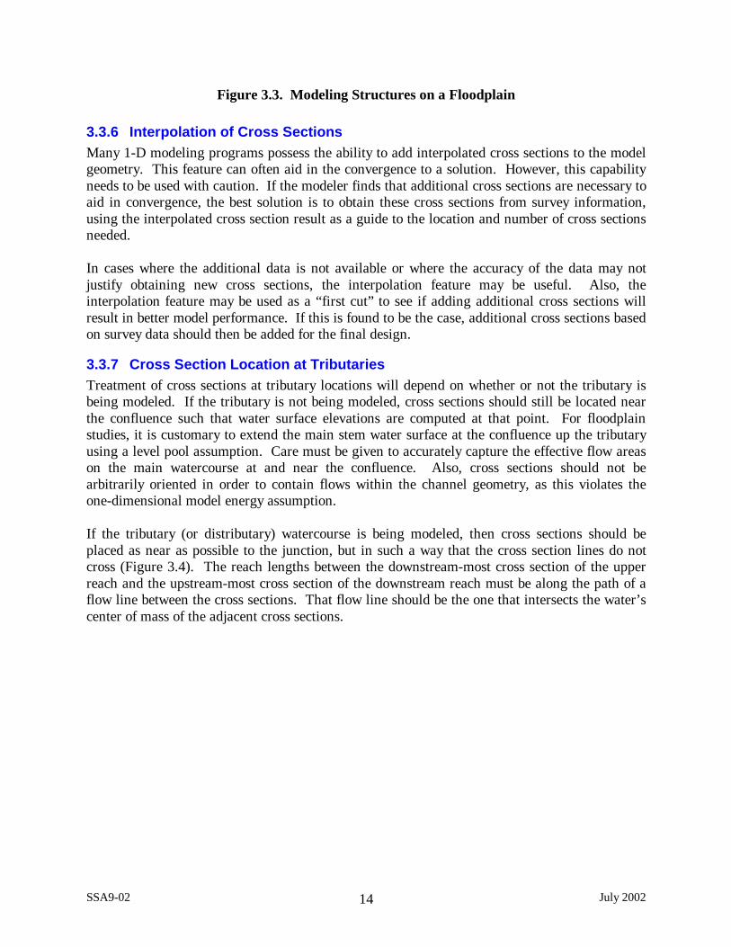
3.3.7 Cross Section Location at TributariesTreatment of cross sections at tributary locations will depend on whether or not the tributary isbeing modeled. If the tributary is not being modeled, cross sections should still be located nearthe confluence such that water surface elevations are computed at that point. For floodplainstudies, it is customary to extend the main stem water surface at the confluence up the tributaryusing a level pool assumption. Care must be given to accurately capture the effective flow areason the main watercourse at and near the confluence. Also, cross sections should not bearbitrarily oriented in order to contain flows within the channel geometry, as this violates theone-dimensional model energy assumption.

If the tributary (or distributary) watercourse is being modeled, then cross sections should beplaced as near as possible to the junction, but in such a way that the cross section lines do notcross (Figure 3.4). The reach lengths between the downstream-most cross section of the upperreach and the upstream-most cross section of the downstream reach must be along the path of aflow line between the cross sections. That flow line should be the one that intersects the water’scenter of mass of the adjacent cross sections.

SSA9-02 July 200215

FigurFigure 3.4. Cross Section Placement at Watercourse Junctions

Figure 3.4. Cross Section Placement at Watercourse Junctions

SSA9-02 July 200216

4. Inflows and Outflows

4.1 Local Inflows and OutflowsMost models have the ability to simulate tributary or distributary watercourses, as well as localinflows and outflows. Local inflows and outflows occur at points in a 1-D model wheredischarge changes due to flow entering or leaving the system and the tributary or distributarywatercourses are not modeled. Local inflows and outflows are handled easily in the model bysimply changing the discharge at a point or points in the watercourse reach. The change isusually determined external to the program.

4.2 Tributaries, Distributaries, and BreakoutsModeling of tributaries is usually straightforward since the discharges from each branchupstream of a junction are combined to define the flow in the reach downstream of the junction.Modeling of distributary flow (Figure 4.1) and breakouts (flow leaving the channel along an ill-defined watercourse) is more complex.

Figure 4.1. Flow Split at a Junction

Reach 1

Reach 3Reach 2

Junction

SSA9-02 July 200217

Some computer programs require the modeler to explicitly define the amount of flow leaving themain watercourse via some external analysis. Other programs (such as HEC-RAS 3.0) willperform iterative calculations using the energy and/or momentum equations to determine howmuch flow will leave the channel. In HEC-RAS, flow may leave the main channel in one of twoways: either by a flow split at a user-defined junction, or by a user-defined lateral weir along awatercourse reach. The latter method mirrors the “split flow method” found in HEC-2. Waterleaving the system via a lateral weir can be brought back (all or a portion of the total) to adownstream location within the model or completely removed from the model.

One simple case of flow leaving the main watercourse and then returning as a tributarysomewhere downstream is the situation of flow around an island (Figure 4.2). With 1-Dmodeling assumptions, the energy at the cross section immediately downstream of the island(River Mile (RM) 10.0 in the figure) will have a unique value, as will the energy at the crosssection immediately upstream of the island (RM 10.8). Calculations to solve for the amount offlow in each reach around the island consist of “balancing” the energy at the upstream end ofeach of the flow paths by an iterative procedure. First a flow split is assumed, and then theenergy at the upstream tip of the island is computed for each of the flow paths. The properdivision of the total flow in each of the reaches is obtained when the energy at the upstream crosssection is the same (within a given tolerance) for each reach.

Figure 4.2. Flow Around an Island (Plan View)

For FEMA studies of tributaries, the downstream starting water surface elevation can be basedupon either normal depth of the tributary or the main stem discharge when the 100-year floodoccurs in the tributary. For that discharge, the water surface elevation of the main stem at thetributary location would then be used as the starting water surface elevation for the tributary.Analyses of the hydrographs (and timing) of the main stem and the tributary must be conducted.The most conservative assumption is usually to use the 100-year water surface elevation of themain stem as the boundary condition for the tributary (coincidental peaks assumption). FEMA

Flow Island

River Mile 10.8

10.610.4 10.2

10.0

SSA9-02 July 200218

37 (FEMA 1995) states that the assumption of coincident peaks may be appropriate if “a) theratio of the drainage areas lies between 0.6 and 1.4, b) the times of peak flows are similar for thetwo combining watersheds, and c) the likelihood of both watersheds being covered by the stormbeing modeled are high.”

For determination of the FEMA regulatory floodway, the downstream starting water surfaceelevation is usually based upon normal depth.

SSA9-02 July 200219

5. Special Topics

5.1 Modeling of Hydraulic StructuresHydraulic structures cause additional energy losses that should be accounted for in the watersurface profile calculations with proper modeling procedures. The information and guidelinespresented are specifically applicable to HEC-RAS and HEC-2; however, the basic concepts and“rules of thumb” are applicable to any 1-D model. The modeler should always refer to theappropriate computer program user’s manual for detailed and specific guidance regarding thatparticular program.

5.1.1 BridgesThe goal of bridge modeling should be to properly account for the energy losses occurringimmediately upstream of the bridge (due to flow contraction), in the bridge structure itself, andimmediately downstream of the bridge (due to flow expansion). It should be noted that, for abridge (and elevated approach roads) that encroach over half of the 100-year floodplain, thehydraulic losses at and near a bridge are due primarily to expansion losses with the contractionloss about the same as the loss at the bridge if there are a modest number of piers. This meansthat the majority of the modeling effort should be expended in correctly locating cross sectionsthat properly capture the expansion and contraction losses.

The modeler should first consider the kind of flow situation being modeled. There areessentially two types of bridge flow situations: Low Flow and High Flow. The bridge flowcomputation method should be selected based on the type of flow.

Low flow exists when the flow through the bridge opening is open channel flow and the watersurface is below the highest point of the low chord (often referred to as the low steel) of thebridge opening.

High flow exists when the flow through the bridge opening is in contact with the maximum lowchord of the bridge deck. When this occurs, the bridge is in pressure flow. If the bridgestructure is overtopped, the bridge is under combined pressure and weir flow. If the approachroadway embankments are overtopped, it is usually considered weir flow.

5.1.1.1 General GuidelinesThe basic requirements for bridge modeling include:

? Bridge Cross Sections: A bridge should be modeled with at least four user-specifiedcross sections. See “Locating Bridge Cross sections” (Section 5.1.1.2.1) for detailedguidance.

? Bridge Geometry: The bridge geometry, both the upstream and downstream faces,should consist of the bridge deck and roadway, abutments, and piers, as appropriate. Forhigh flows that are expected to overtop the bridge, the bridge railing and the approachroadway embankment should be modeled as a part of the bridge deck.

SSA9-02 July 200220

? Ineffective Flow Areas: Ineffective flow areas upstream and downstream of the bridgeshould be based on the type of flow situation being modeled. See “Locating BridgeCross sections” for detailed guidance.

? Contraction and Expansion Losses: Flow contracts as it enters a bridge opening andexpands on its way out. Appropriate contraction and expansion coefficients should beused to model energy losses associated with the flow transition through a bridge. Theloss due to expansion of flow is typically larger than the loss due to contraction of flow.Abrupt transitions result in larger losses compared to gradual transitions.

? Selection of Modeling Approach: The modeler must consider the choice of bridgemodeling method based on the type of flow (low flow or high flow) situation. The mostbasic solution methods available include the energy-based method, the momentum basedmethod, and empirical methods.

5.1.1.2 Specific GuidelinesThe following specific guidelines should be followed for modeling bridges.

5.1.1.2.1 Locating Bridge Cross SectionsA plan view of the basic cross section layout is shown in Figure 5.1. The arrows show the actualflow path and the shaded areas shows the ineffective flow areas for non-overtopping conditions.

Cross Section 1 should be located sufficiently downstream from the structure so that the flow isnot affected by the structure (i.e., the flow has fully expanded). This distance (also called theexpansion reach length) should generally be determined by field investigation during significantflow conditions.

If a field investigation is not possible under these conditions, the study entitled “Flow Transitionsin Bridge Backwater Analysis” (USACE, 1995) may be used. Use of the method recommendedin the report requires an iterative process and a suggested starting expansion ratio of 3:1(longitudinal to lateral distance or three times the average of the distance from A to B and C to Din Figure 5.1). Field studies (USACE, 1995) found expansion ratios varying from 0.5 to 4longitudinal units for each lateral unit.

The expansion distance varies depending upon the degree of constriction, the shape of theconstriction and the magnitude and velocity of the flow. If the expansion reach requires a longdistance, then intermediate cross sections should be placed within the expansion reach in order toadequately model friction losses.

For non-overtopping flow situations, the ineffective flow area of the intermediate cross sections(between cross sections 1 and 2), as depicted by the shaded areas in Figure 5.1, should bemodeled appropriately.

Cross Section 2 is located a short distance downstream from the bridge, commonly placed at thedownstream toe of the road embankment. This cross section should represent the effective flowarea just downstream of the bridge.

SSA9-02 July 200221

Figure 5.1. Basic Cross Section Layout of Bridge Cross Sections (after USACE, 2001)

For low flow and pressure flow conditions, when the bridge abutments and roadwayembankments obstruct the entire floodplain, the overbank areas should be modeled as ineffective(represented by the shaded area between cross sections 1 and 2). For high flows overtopping thebridge deck, the area outside the main bridge opening may become effective flow and should beincluded as an active flow area.

Cross Section 3 should be located a short distance upstream from the bridge, commonly placed atthe upstream toe of the road embankment. The distance between cross section 3 and the bridgeshould only reflect the length required for the abrupt acceleration and contraction of the flow thatoccurs in the immediate area of the opening. Cross section 3 represents the effective flow areajust upstream of the bridge. Similar to cross section 2, for low flow and pressure flow conditionsand when the bridge abutments and roadway embankments obstruct the entire floodplain, theoverbank areas should be modeled as ineffective (represented by the shaded area between cross

FlowDirection

4

3

2

1

A B C D

IneffectiveFlow Areas

SSA9-02 July 200222

sections 3 and 4). For high flows overtopping the bridge deck, the area outside the main bridgeopening may become effective flow and should be included as an active flow area.

Cross Section 4 should be located where the flowlines are approximately parallel and the crosssection is fully effective. Because flow contractions can occur over a shorter distance than flowexpansions, a suggested starting contraction ratio, generally adopted by the Corps of Engineers,is 1 longitudinal to 1 lateral distance (one times the average of the distance from A to B and C toD in Figure 5.1).

In addition, the study entitled “Flow Transitions in Bridge Backwater Analysis” (USACE, 1995)may be used. Use of the method recommended in the report requires an iteration process andagain, a suggested starting contraction ratio is 1 longitudinal to 1 lateral distance (one times theaverage length of the side constriction caused by the structure abutments). Field studies(USACE, 1995) found contraction ratios varying from 0.3 to 2.5 longitudinal units for eachlateral unit.

5.1.1.2.2 Modeling Low FlowThe following guidelines should be followed for selecting the modeling approach for low flowsituations:

1) In cases where the bridge piers are a small obstruction to the flow, and friction losses arepredominant (e.g., a very wide opening or very few piers), the energy based method orthe momentum method may be used.

2) In cases where pier losses and friction losses are both predominant, the momentummethod should be used, but other methods may also be applicable.

3) When flow passes through critical depth within the vicinity of the bridge, both themomentum and energy methods may be used.

4) For supercritical flow, both the energy and the momentum method may be used. Themomentum-based method may be better at locations that have a substantial amount ofpier impact and drag losses.

In HEC-RAS, the user may select any one of the available loss methods, or select multiplemethods and have the program use the result with the highest energy loss.

5.1.1.2.3 Modeling High FlowIn general, for high flows the energy based method is applicable to the widest range of problems.The following guidelines should be followed for selecting the modeling approach for high flowsituations:

1) When the bridge deck is a small obstruction to the flow, and the bridge opening is notacting like a pressurized orifice (e.g., the bridge is highly submerged), the energy-basedmethod should be used.

SSA9-02 July 200223

2) When the bridge deck is a large obstruction to the flow and a backwater is created due tothe bridge deck, the pressure and weir method should be used.

3) When the bridge is overtopped and the water going over top of the bridge is not highlysubmerged by the downstream tailwater, the pressure and weir method should be used.

4) When the bridge is highly submerged, and flow over the road is not acting like weir flow,the energy-based method should be used.

5.1.1.2.4 Perched BridgesA perched bridge is one for which the road approaching the bridge is at the floodplain groundlevel and only in the immediate area of the bridge does the road rise above ground level to spanthe watercourse. A typical flood-flow situation with this type of bridge is low flow under thebridge and overbank flow around the bridge.

The assumption of weir flow is not justified for this situation because the road approaching thebridge is usually not much higher than the surrounding ground. A solution based on the energymethod (standard step calculations) would be better than a solution based on weir flow when alarge percentage of the total discharge is in the overbank areas.

5.1.1.2.5 Low Water BridgesA low water bridge is designed to carry only low flows under the bridge and flood flows arecarried over the bridge and road.

When modeling this bridge for flood flows, the anticipated solution is a combination of pressureand weir flow; however, if the tailwater is going to be high, it may be better to use the energy-based method. HEC-RAS automatically uses the energy-based method when submergence is 95percent or higher.

5.1.1.2.6 Skewed BridgesSkewed bridge crossings are generally handled by making adjustments to the bridge dimensionsto define an equivalent cross section perpendicular to the flowlines.

Skewed crossings with angles up to 20 degrees do not show objectionable flow patterns(Hydraulics of Bridge Waterways", Bradley, 1978). Bridges with a skew angle greater than 30degrees should be modeled by adjusting the bridge dimensions to represent the projected lengthof the bridge deck, and if necessary, the projected width of the bridge piers, perpendicular to theflow direction.

5.1.1.2.7 Parallel BridgesParallel bridges are usually caused by construction of divided highways or highway and railroadbridges side by side. The hydraulic losses through the two structures may be between one andtwo times the loss for one bridge (Bradley, 1978).

If the parallel bridges are very close to each other, and the flow will not be able to expandbetween the bridges, they should be modeled as a single bridge.

SSA9-02 July 200224

If there is enough distance between the bridges in which the flow has room to fully expand andcontract, the bridges should be modeled as two separate bridges.

If the bridges are so close that full expansion and/or contraction is inhibited, care should beexercised in depicting the expansion and contraction of flow between the bridges.

5.1.1.2.8 Multiple Bridge OpeningsBridges with side relief openings and separate bridges over a divided channel, with possibledifferent control elevations, are examples of multiple opening problems. The hydraulic analysisof multiple openings is a complex hydraulic problem.

Computer programs such as HEC-RAS have the capability to model multiple openings. Analternative approach is to model the flow paths of each opening as a separate reach.

5.1.1.2.9 Modeling Floating Debris on PiersField reconnaissance should be performed to determine the potential for trash, trees, and otherdebris that may accumulate on the upstream side of a pier during high flow events. Debris mayblock a significant portion of the bridge opening and should be modeled by increasing thethickness of the piers. HEC-RAS has an option to model floating debris on piers.

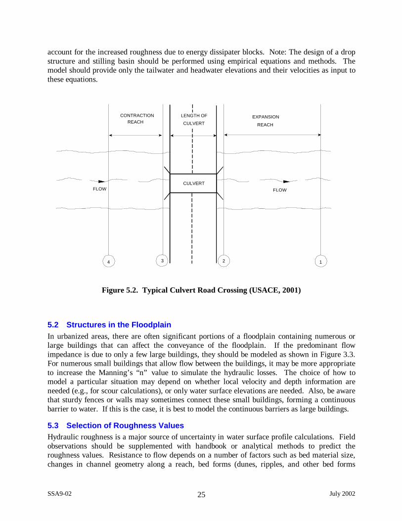
5.1.2 CulvertsCulvert modeling is similar to bridge modeling except that culvert hydraulics equations are usedto compute inlet control losses. The Federal Highway Administration's (FHWA, 1985) standardequations for culvert hydraulics are the most commonly used. Figure 5.2 illustrates the crosssections required for a culvert model.

Most hydraulic computer programs capable of modeling culverts use the concepts of inlet controland outlet control. The most common culvert types are circular pipe culverts and box culverts.A typical box culvert road crossing is similar to a bridge in many ways with the walls and roof ofthe culvert corresponding to the abutments and low chord of the bridge, respectively.

The layout of cross sections, the use of the ineffective areas, the selection of loss coefficients,and most other aspects of bridge analysis are applicable to culverts as well. In addition, culvertequations require entrance and exit loss coefficients.

5.1.3 WeirsInline hydraulic structures such as weirs, gated spillways, and drop structures (structures acrossthe main watercourse), are typically modeled with empirically based equations such as the weirequation. Computer programs such as HEC-RAS are capable of modeling such structures.

A minimum of four cross sections are required. For drop structures, the cross sections should beclosely spaced where the water surface and velocity is changing rapidly. If a sloping drop is tobe modeled, additional cross sections should be placed along the slope in order to model thetransition from super-critical to sub-critical flow. Several cross sections should also be placed inthe stilling basin and the energy dissipation area in order to correctly locate where the hydraulicjump will occur. Manning’s roughness values should be increased inside the stilling basin to

SSA9-02 July 200225

account for the increased roughness due to energy dissipater blocks. Note: The design of a dropstructure and stilling basin should be performed using empirical equations and methods. Themodel should provide only the tailwater and headwater elevations and their velocities as input tothese equations.

FLOWFLOWCULVERT

1234

EXPANSIONCULVERT

LENGTH OFREACH REACH

CONTRACTION

Figure 5.2. Typical Culvert Road Crossing (USACE, 2001)

5.2 Structures in the FloodplainIn urbanized areas, there are often significant portions of a floodplain containing numerous orlarge buildings that can affect the conveyance of the floodplain. If the predominant flowimpedance is due to only a few large buildings, they should be modeled as shown in Figure 3.3.For numerous small buildings that allow flow between the buildings, it may be more appropriateto increase the Manning’s “n” value to simulate the hydraulic losses. The choice of how tomodel a particular situation may depend on whether local velocity and depth information areneeded (e.g., for scour calculations), or only water surface elevations are needed. Also, be awarethat sturdy fences or walls may sometimes connect these small buildings, forming a continuousbarrier to water. If this is the case, it is best to model the continuous barriers as large buildings.

5.3 Selection of Roughness ValuesHydraulic roughness is a major source of uncertainty in water surface profile calculations. Fieldobservations should be supplemented with handbook or analytical methods to predict theroughness values. Resistance to flow depends on a number of factors such as bed material size,changes in channel geometry along a reach, bed forms (dunes, ripples, and other bed forms

SSA9-02 July 200226

relating to flow regime), and vegetation type and density. Roughness will also vary with depth,decreasing as the water depth becomes much greater than roughness elements (vegetation, bedmaterial, bed forms, etc.) Therefore, the resistance to flow will vary from season to season andyear to year. Because changes will occur over time, a range of roughness values should beconsidered and a sensitivity analysis is recommended to show how the uncertainty in theroughness value affects the computed water surface elevation and/or velocity.

Consideration should also be given to the overall goal of the model. When velocity is a criticalparameter (e.g., in bank protection design), a roughness value on the lower end of the rangeshould be used, and when the water surface elevation is more critical (e.g., in levee design), ahigher roughness value should be used.

Handbook methods involve the use of “calibrated photographs” and other subjective methods toassociate hydraulic roughness values with conditions observed and anticipated in the projectreach. Chow (1959), Barnes (1967), and more recently Hicks and Mason (1998) are thedominant sources of calibrated photographs. Arcement and Schneider (1989) published a reportwith photographs to help estimate roughness values for vegetated floodplains.

Analytical methods are physically based equations that relate hydraulic roughness to theeffective surface roughness and irregularity of the surface boundaries (Example: MoodyDiagram). Notable equations that can be used are the Strickler equation, Keulegan’s rigid bedequations, the Iwagaki relationship, the Limerinos equation, and others (e.g., USACE, 1994).

For roughness value estimation, the following publications specific to Arizona channels may beconsulted:

1) Estimated Manning's Roughness Coefficients for Stream Channels and Floodplains inMaricopa County, Arizona, (Thomsen and Hjalmarson, 1991)

2) Roughness Coefficients for Stream Channels in Arizona (Albridge and Garrett, 1973)3) Verification of Roughness Coefficients for Selected Natural and Constructed Stream

Channels in Arizona (Phillips and Ingersoll, 1998)

For the design of vegetated flood control channels, the modeler must use an appropriateroughness value to account for fully vegetated conditions. One reference specific to Arizonawatercourses is “Method to Estimate Effects of Flow-Induced Vegetation Changes on ChannelConveyances of Streams in Central Arizona” (Phillips et al., 1998).

A word of caution in using Manning’s “n” values based upon a field reconnaissance. When themodeler inspects a watercourse to judge its roughness, the physical state of the system when it isinspected is not necessarily the physical state the system would be under design conditions.FEMA studies are usually based upon a 100-year flood, and the roughness of the watercourseduring such an event would be drastically different than what is seen in the field. What is seen inthe field may be several years after a major flood event and it may have “healed” or been workedover by smaller floods, hiding any evidence of how the actual situation was during high flowevents. It is suggested that if the roughness is based upon vegetative resistance, a shear stressanalysis should be conducted to check if the vegetation’s critical shear stress is exceeded by the

SSA9-02 July 200227

actual shear stress. Conversely, if a plane streambed is observed and only the grain resistance isused to obtain the “n” value, the actual resistance may be higher under design floods becausedunes or ripples may form and become important additional components in determining theManning’s “n.”

5.4 BendsCowan (1956) has suggested that the Manning’s “n” value can be adjusted to simulate theadditional hydraulic loss due to bends in the watercourse. He suggests modification to theoverall n value based upon the severity of the bend. However, an adjustment is generally notneeded for a watercourse with a ratio of the radius of curvature to active channel width greaterthan 10. Also, some methods used for determining the roughness value (e.g., “calibratedphotographs”) implicitly include energy losses due to bends. Changing expansion andcontraction coefficients to simulate bend losses is not only inappropriate, there are no guidelineson what are reasonable values to use for various degrees of bend severity. Adjustments to thefloodplain due to superelevation at bends are not suggested in FEMA studies; however, they arecommonly used for designing flood control protection such as artificial channels and levees andfor determining increased shear stresses for streambank protection measures.

5.5 Modeling Supercritical and Mixed FlowAll 1-D models will compute solutions for subcritical flow conditions. Many will also computesupercritical flow. A few, such as the steady flow module of HEC-RAS, will compute “mixedflow,” i.e., both sub- and supercritical flow occurring in a single water surface profile. TheArizona State Standard on Supercritical Flow (SS3-94) should be referred to when modelingsupercritical flow situations. Note: For FEMA floodplain studies, supercritical flow results fromhydraulic models will not be accepted by FEMA for delineation of floodplains or floodwaysunless the watercourse was specifically designed for and adequately protected againstsupercritical flow conditions under the 100-year flood discharge. Also, if the watercourse wasdesigned to accommodate supercritical flow, the floodplain becomes the floodway since theconcept of a regulatory floodway based upon an “allowable rise” is not appropriate forsupercritical situations. This point is also emphasized in SS3-94.

5.6 Floodplain Delineation ModelsDelineation of floodplains for a Flood Insurance Study (FIS), letter of map revision, or otherpurpose is a common reason for developing/updating a hydraulic model of a watercourse. FISrequirements are provided in the FEMA 37 document (FEMA, 1995) and other State Standards.New FIS’s and revisions to existing studies should follow the guidelines in these publicationsand the modeling procedure given in Section 6.3 of this standard.

5.7 Modeling of Pit Areas (sand & gravel mining) and LakesSand and gravel extraction operations result in pits or depressions that can be located in-channelor off-channel. In-channel pits are less common because of the environmental impacts, therelated regulations, and permitting procedures. Off-channel pits are more common and arelocated in the overbank area adjacent to the main channel. Off-channel pits are typicallyseparated from the main channel by levees. Similarly, natural or man-made lakes or depressionscan be found either in-channel or off-channel. There is essentially no difference between lakesand pits with regard to hydraulic computer modeling for floodplain studies.

SSA9-02 July 200228

5.7.1 In-Channel PitsWith regard to a hydraulic study involving an in-channel pit, one of the important factorsinfluencing the type of model selected is the size of the pit. If the pit is very large in comparisonto the average channel size (such as a lake), storage and its effect on flow attenuation will be amajor consideration. In that case, an unsteady flow analysis (which considers the finite volumeof water in the hydrograph) may be the best choice.

On the other hand, the purpose of the study may govern the kind of model selected. If thepurpose is to delineate floodplains, it might be of interest to compute the most conservative(maximum) water surface elevations. In such a case, a steady flow model can be selected andthe water surface elevation computed by completely ignoring the pit (filling in the pit) in thecross section.

For example, the steady flow module of HEC-RAS can be used to model the pit as a blockedobstruction, flush with the bed surface. Such a method would eliminate the additionalconveyance in the pit and result in higher water surface elevations. Blocking conveyance in thepit area by using high Manning’s “n” values is not recommended because an unrealistically highroughness will be used for a whole range of flows (unless the model has the ability to vary theroughness with stage or discharge). In general, if conservative results are desired, in-channel andoff-channel pits should be modeled as blocked obstructions flush with the adjacent streambed.The “n” values used for the pit area should be consistent with the roughness values assignedimmediately upstream and downstream of the pit area.

Other factors to consider are the magnitude of the flood and the potential for sediment transport.If the pit is small, it may be reasonable to assume that the pit may be filled with sediment duringa large flood. This assumption would then become the basis for ignoring isolated depressionsand smoothing out the cross section for use in a steady flow analysis. On the other hand, if aflood of small magnitude were being modeled, it may be necessary to account for the presence ofthe pit.

Another factor that could be considered is the shape of the storm hydrograph. The hydrographshould be examined in order to determine if the pit will be filled before the peak of the stormhydrograph arrives at the location of interest. The pit will most likely be filled if the hydrographis slow to peak and has a rising limb with a volume close to or greater than that of the pit. In thiscase, it may be justified to assume that the pit can be blocked off and does not possess anyconveyance during the modeling of the peak discharge in a steady flow analysis.

5.7.2 Off-Channel PitsFor off-channel pits, the major considerations are the presence of levees, the size of the pit, andthe magnitude of the flood. If the levees separate the main channel from the pits and areassumed to hold during the flood under consideration, the area beyond the levees can be ignoredor blocked off. If the levees are failed or if the flood is large enough to overtop the levees, twosituations should be considered.

In one situation, the pit area will be storing water but not actively conveying flow downstream.In this case, the pit should be modeled as an ineffective flow area.

SSA9-02 July 200229

In the second situation, the pit area is actively conveying flow and will have to be modeled as apart of the overbank flow path. If a steady flow model is being used, a split flow analysis shouldbe conducted to determine the breakout discharge from the leveed main channel. Then, based onthe overbank flow conditions, the overbank area including the pit can be modeled as a separatereach conveying the breakout flow. If an unsteady flow model is being used, the pit in theoverbank area can be modeled as a storage cell defined by an elevation-storage curve and/or as aseparate flow path similar to the discussion for the steady flow model.

In summary, a steady flow analysis should be selected by ignoring the pit if conservative resultsare desired and the pit is small. An unsteady flow analysis should be considered when floodstorage is a major consideration such as for large in-channel pits and lakes or when there is thepossibility of flow through or over levees into depressed floodplains containing a large pit.

5.7.3 Model Input Data ConsiderationsModel selection is followed by the collection of model input data. At a minimum, such dataincludes topographic maps or cross section surveys, as-built plans for bridges, or other in-channel structures. Proper consideration must be given to the selection of the scale and contourinterval of the topographic map. For example, if an off-channel pit is being considered as astorage area, elevation-volume data of the pit must be obtained from the topographic map. Inthis case, it may be necessary to obtain a map with a 1-foot or a 2-feet contour interval. Often,the mapping costs constitute a significant portion of the total cost of the modeling study.

The most important task before data entry to the hydraulic model is the proper orientation andspacing of the cross sections and review of the cross section data. Cross sections should alwaysbe aligned perpendicular to the direction of flow for the event(s) being modeled and spaced suchthat major grade breaks in the channel profile are represented. This is particularly important ifthe pits or related activities change the natural flow patterns. Section 3.3 provides additionalinformation on cross section placement and orientation.

For modeling large pits and lakes, an appropriate number of cross sections should be selected toproperly represent the change in pit dimensions. At a minimum, there should be a cross sectionlocated at the beginning and the end of the pit with an additional cross section at the widest partof the pit. The model will then “see” the pit as a diamond shape in planform. If this shape doesnot adequately describe the actual shape of the pit, then additional internal cross sections may beneeded.

SSA9-02 July 200230

6. FLOODWAY METHODS

6.1 GeneralThe Federal Emergency Management Agency (FEMA) administers the National Flood InsuranceProgram (NFIP). Under this program, a regulatory floodway is defined as the channel of awatercourse and the adjacent land areas that must be reserved in order to discharge the base floodwithout cumulatively increasing the water surface elevation by more than a designated height.The area between the limits of the regulatory floodway and the inundation limits for the baseflood is called the floodway fringe. The base flood is the event having a 1% chance of occurringin any given year (also called the “100-year” flood). The designated height is one foot (themaximum allowed by FEMA) or a lesser amount specified by a local agency. For near-criticalor supercritical flows, the height is applied to the rise in the energy grade line rather than the risein water surface elevation.

The local community is responsible for prohibiting encroachments in the regulatory floodway(including fill, new construction, and other improvements) unless it has been demonstratedthrough hydrologic and hydraulic analyses, performed in accordance with standard engineeringpractice, that the proposed encroachment would not result in any increase in flood levels duringthe occurrence of the base flood discharge. Proposed encroachments in a designated floodway,which result in an increase in the base flood elevations (BFE’s), must be approved by FEMA.Such encroachments must comply with §60.3.d.4 and §65.12 of the NFIP regulations. Aschematic of floodway definitions is shown in Figure 6.1.

Figure 6.1. Schematic Showing Floodway Definitions

SSA9-02 July 200231

6.2 Floodway DevelopmentThis section provides a general procedure to evaluate the impact of a development (herebyreferred to as “floodway development” or “floodway encroachment”) inside a regulatoryfloodway limit. Floodway development has the potential to obstruct flow. But since suchdevelopment, by virtue of being in the regulatory floodway, is subject to the “no-rise” criterionfor base flood elevations (explained in greater detail later), it usually requires the implementationof terrain modifications (hereby referred to as “compensatory actions”) to insure that flood levelsdo not rise as a result of the floodway development. There are two possible ways to achieve thecompensatory actions: by excavation, or by the reduction of the roughness coefficient. Note:Some local floodplain management ordinances regulate what uses are allowed in a floodway.Prior to modeling a development in a floodway, the modeler must check with the local floodplainmanagement office.

FEMA generally requires that the same software package used for the original Flood InsuranceStudy also be used to model the modifications to the floodway. However, newer and improvedversions of the same software package are often available. FEMA generally permits the use ofnewer software versions for development studies. However, newer software versions willsometimes compute different water surface elevations than previous versions. For example,Version 3.0 of HEC-RAS will often give slightly different water surface elevations than identicalmodels run under Version 2.2 of HEC-RAS. Therefore, a “duplicate effective” model needs tobe created, which is a copy of the original model (the “effective model”) with water profiles re-calculated with the newer software version. For uniformity, the “duplicate effective” modelshould be created whether the software version has changed or not.

6.3 Modeling ProcedureThe general procedure recommended for floodway encroachment analysis is a series of 5different models: Duplicate Effective, Corrected Effective, Pre-Project (Existing) Conditions,Post-Project without Compensatory actions, and Post-Project. Each model is an incrementalmodification of the model preceding it. Each model also has two different versions: theunencroached version (no floodway) and the encroached version (with floodway). All thesemodels are run using the same version of the software. A conceptual description of each modelis provided below.

6.3.1 Duplicate Effective ModelThe Duplicate Effective model is a copy of the original FEMA Flood Insurance Study model(called the “effective model”), where the water surface profiles are computed using the versionof the software (usually the most recent version) that will be used for the remainder of thefloodway development study. This model should have all the original encroachment stations sothat the model can be run in the unencroached and in the encroached versions. If the softwareversion for the floodway development study is not identical to that used in the original FloodInsurance Study, the water surface elevations in this model might differ from those in theEffective model. If this is the case, the reasons for the differences should be established. Theresults from the newer software version are generally accepted by FEMA.

SSA9-02 July 200232

6.3.2 Corrected Effective ModelThe Corrected Effective model is the Duplicate Effective model with the followingmodifications:

1) It contains additional cross sections that will be used in the Pre- and Post-Project models(e.g., if a bridge is proposed, the 6 cross sections needed for bridge modeling should beadded). In the corrected effective model, the cross section geometry and “n” valuesshould reflect the conditions at the time the Flood Insurance Study was conducted. Thatmeans that no changes to the topography since the Flood Insurance Study was conductedare to be considered.

The encroachment stations (floodway limits) for all the added cross sections must bedetermined. This is done by plotting the new cross sections on the Flood Insurance Ratemap and measuring the floodway limits (which are the encroachment stations) using thismap.

2) Any conceptual modeling errors in the original FEMA model can also be corrected in thismodel with the reasons for the corrections well documented. However, unless the errorsare significant, it is suggested that no additional modifications be made.

It is frequently the case that the addition of cross sections in this model will cause changes in thecalculated water surface elevations. This brings up two issues:

1) The base flood elevations change; i.e., the water surface elevations in the unencroachedmodel. The addition of cross sections alone will usually cause the model to computedifferent water surface elevations than those computed in the Duplicate Effective model,in the cross sections upstream of the new cross sections.

2) The encroached, or surcharged, water surface elevations change; i.e., the water surfaceelevations in the case where the floodway fringe is excluded from the flow area. Thecriterion that must be met is that the encroached water surface elevations must be onefoot or less than the unencroached water surface elevations at all cross sections. If these“surcharges” are greater than 1’, then the floodway must be redelineated.

6.3.3 Pre-Project (Existing) Conditions ModelThe Corrected Effective model cross sections are modified to reflect any changes in thetopography that have occurred since the Flood Insurance Study was conducted. Thesemodifications apply to the cross sections added in the Corrected Effective Model as well as to theoriginal cross sections from the Effective model. Changes that are near the proposed project siteneed to be incorporated in the Existing Conditions model. Changes at cross sections not near theproposed site typically need not be modified.

Generally, the Existing Conditions model will not differ from the Corrected Effective modelunless there has been some natural deposition or erosion. Any man-made changes within thefloodway should have been submitted to FEMA for approval, and the Flood Insurance Studymodel should have been updated to reflect these changes. If there have been undocumented

SSA9-02 July 200233

changes inside the floodway since the Flood Insurance Study, this would be a special caserequiring consultation with FEMA and the community on how to proceed with the developmentstudy.

6.3.4 Post-Project Without Compensatory Actions ModelFor the Post-Project without Compensatory actions model, the cross sections are modified toreflect the new structure or project. Compensatory actions are not included in the model. Thisintermediate model is not required by FEMA, but is recommended for clarity.

6.3.5 Post-Project Conditions ModelFor the Post-Project Conditions model, cross sections are modified to reflect the compensatoryactions needed to result in a “no-rise” condition, explained in the following section.

6.4 “No Rise” ConditionThe “no rise” condition means that the water surface elevations at every cross section in the Post-Project unencroached model cannot exceed the water surface elevations at each correspondingcross section of the Existing Conditions unencroached model. Satisfying this conditiondemonstrates that the project will not cause a rise in the BFE’s.

An additional consideration is the effect of the development on the encroached water surfaceprofile. This could occur, for example, if a building was added in the floodway, and anexcavation was conducted in the floodway fringe to compensate. In that case, the BFEcalculations (which are unencroached) might result in no increase of the water surface, but theencroached water surface elevations could rise more than one foot because the compensatoryaction in the fringe would provide no additional conveyance in the regulatory floodway.

Except for encroachments in designated floodways, the NFIP regulations permit a rise in theencroached water surface elevations as long as the surcharge remains less than or equal to onefoot. However, the local community may wish to apply the no-rise criteria to the encroachedprofile for several reasons. For example, any compensatory action taken in the floodway fringewould need to be permanent, causing an enforcement issue to maintain properties outside thefloodway. Also, new developments in the floodway fringe could eliminate the benefit providedby a compensatory action, making it difficult to guarantee the permanent hydraulic effectivenessof the compensatory action.

Therefore, it is recommended that all compensatory measures be located inside the floodway,that they be “permanent” (e.g., maintained and hydraulically connected) measures, and that the“no rise” condition be applied to the encroached Post-Project model as well as the encroachedExisting Conditions model.

6.5 Cumulative EffectsThe cumulative effects of development in the floodplain should not violate the “no rise”condition described in the preceding section. Where no floodway has been designated,conducting a re-study and developing a floodway usually addresses the cumulative effects.Revised discharges and updated topography may be required for the re-study.

SSA9-02 July 200234

6.6 Generation of Additional Cross sectionsGenerally, numerous cross sections must be added in the Post-Project model (these cross sectionsappear in the Corrected Effective and subsequent models as well) to properly model thefloodway development. For example, in the case of a building added in the floodway, aminimum of six cross sections would need to be added to properly model the building.Sometimes even more cross sections must be inserted for developments with overlappinghydraulic effects (see Figure 3.3).

Such additional cross sections can be surveyed, or they can be developed from topographicmaps. Unless the modeling conditions are very simple, however, it is often not easy to determinewhere cross sections will be needed. Therefore, the recommended procedure is to develop atopographic map of the area if none exists.

Sometimes, in order to create all the cross sections needed for the hydraulic model, crosssections are copied from other cross sections nearby. This practice should be restricted tocopying from cross sections that are very close and where there would not be any significantchanges in shape or elevation between the two cross sections. Such actions should bedocumented within the model and report. In general, FEMA does not accept copied crosssections for floodplain and floodway determination.

6.7 Reducing RoughnessOften, an expedient way to lower the calculated water surface elevations is to reduce flowresistance by selective clearing and landscaping, thereby reducing Manning’s “n” values in themodel at or near the floodway development site. FEMA requires that a certified maintenanceplan be submitted (FEMA, 1990) when this method is pursued.

Reduction of roughness can be achieved, for example, through changes in landscaping orthrough paving. However, even with certified maintenance plans, reductions in roughnessachieved through landscaping must be viewed skeptically. Due consideration should begiven to the long-term costs of monitoring the modifications, the funding mechanism for meetingthe costs, and the likelihood of the permanence of the modifications. Modifications not subjectto high maintenance, such as paving with concrete, provide more confidence in their durability.Whatever the method used to reduce roughness, such a reduction usually results in increasedchannel velocities. The effect of the new velocities on channel banks and structures needs to beconsidered.

Increases in conveyance can also be more reliably and permanently achieved through excavationand grading. The excavation must be of such size and extent that it will not act as merely adepression, but rather as a free-flowing conveyance element during times of flooding. However,in areas of high sediment transport rates, the excavated area may be filled after major storms.Therefore, if this situation is highly probable, periodic surveys may be needed to assure therequired conveyance is still available.

6.8 Comparison of ConveyancesA method using the comparison of conveyances to analyze a development inside a floodway isdetailed in a FEMA memo from the administrator of the Federal Insurance Administration dated

SSA9-02 July 200235

October 31, 1990. This memo implies that a backwater calculation will nevertheless be requiredin addition to the conveyance calculations. FEMA requires a backwater calculation using acomputer model. Therefore, the comparison of conveyances can only be considered an auxiliaryto a backwater calculation, not a substitute.

The inclusion of conveyance comparisons is a courtesy to FEMA. The comparison should bebetween the conveyance of the encroached Existing Conditions model and that of the encroachedPost-Project model. These conveyances can be extracted directly from the respective computermodels. Conveyances should be compared in every cross section where there is a geometricand/or roughness difference between the Existing Conditions Model and the Post-Project model.

In a “no-rise” scenario, the conveyance in the Post-Project model will generally not differ fromthat of the Existing Conditions model, but this is not always the case. The post-projectconveyances at some sections could decrease because of compensatory actions achieved atdownstream cross sections. Alternately, the compensatory actions might have been taken outsidethe floodway (a practice already discussed that is not recommended).

Note: A decrease in conveyance would not be grounds by FEMA for the rejection of theproposed development. There might be no increase in water surface elevations from theEffective to the Post-Project Models, but there may be decreases in conveyances at some crosssections. Because a conveyance increase could signal an error in the model, and may beconsidered a “red-flag,” it is recommended that an explanation of how the “no-rise” conditioncould be achieved under such circumstances.

SSA9-02 July 200236

7. Good Modeling PracticeHydraulic models require large amounts of data and can produce misleading results withoutproper planning, organization, and execution. A well-managed analysis can save time andmoney. This section emphasizes good modeling practices that can increase the efficiency of themodeling effort and improve the quality of the results.

7.1 Model DocumentationProper model documentation is perhaps one of the most important and yet one of the mostneglected aspects of hydraulic modeling. Experienced modelers understand that good modelingpractice also includes proper documentation and file management. A properly documentedmodel can save much time and effort in the long run and helps expedite the review process.

Since hydraulic models are based upon accurate depiction of the watercourse geometry, it isimperative that the horizontal and vertical accuracy of the survey is adequately described. Inaddition, the vertical datum used should be provided in the report and any rectification ofgeometric data sources using different datum should be described in detail.

The report should include topographic maps with cross sections overlaid on them, including theirorientation. Also, to assist the reviewer, it is suggested that the flowlines and ineffective flowareas in relation to the cross sections be shown on topographic maps.

A modeling project involves the development of computer model input and output files usuallycopied on a floppy diskette or CD and included with a project report. However, diskettes or CDsfrequently get separated from the reports, and without proper documentation the input data filesare practically meaningless. Therefore, basic information should always be included in the inputdata files and cross-referenced with more detailed explanation in the report.

If the modeling effort involves several plans with multiple input data files, each file shouldcontain enough documentation to explain the differences between the input files. It is also usefulto name input data files in a creative and unique manner that helps to quickly identify the natureof the plan or model run.

All input data files should contain basic information such as the following: the name and locationof the project, the name of the watercourse, the name of the modeler, the company the modelerworks for, the address and phone number of the company/modeler, the date of the run, the inputfile name, and a brief description of the main purpose of the run. Additional documentation suchas model source data, explanatory comments on warning messages, and notes on modelingdecisions, may also be included. At the conclusion of the modeling exercise and after thenumerical output has been checked, the modeling notes in the input data file should be reviewed,and any unnecessary comments that could cause confusion to a reviewer should be removed.

Many modeling programs can accommodate comments by the modeler in the program inputand/or output. Frequent comments can greatly aid a reviewer, as well as anyone who uses themodel in the future.

SSA9-02 July 200237

Project reports should contain a detailed discussion of the model input and output along withreference to the model input data filenames, where necessary. For projects that involve multipleinput data files, the report should include an appendix that contains a list of all the input datafiles and a brief description of each file. The Arizona State Standard on Flood Study TechnicalDocumentation (SS1-97) should be referenced for more information.

7.2 Common ErrorsThis section describes the checks for common modeling errors in typical floodplain delineationstudies. A review of errors related to special computations such as bridges, split flowoptimization, junction analysis, and floodway computations are addressed elsewhere in thisattachment.

A hydraulic analysis begins with properly laid out cross sections and estimates of channelroughness and other hydraulic parameters. Tasks such as cross section layout may seemmundane, but should always be supervised by an experienced modeler. This is especially truefor floodplains in the arid southwest where the flow paths are sometimes hard to determine. Thecross section spacing should be determined based on the change in the slope of the groundprofile of the watercourse as well as the change in the width of the watercourse. In general, thecross section spacing is determined by the need to adequately account for the energy losses(friction, flow expansion, and flow contraction) between consecutive cross sections.

Generally, the most obvious errors that appear in the model output should be eliminated first. Ina HEC-2 analysis, these errors may show up as messages in the EDIT-2 output or at the end ofthe HEC-2 output file. In a HEC-RAS analysis, these may show up in the “errors, warnings, andnotes” window.

After correcting the obvious errors, a detailed review of the graphical and tabular output(summary tables) should be conducted. The graphical output is especially useful in locatinglarge changes in water surface elevation, top-width, slope, or velocity. Sudden changes inhydraulic parameters should be based on physical evidence and be explainable in a logicalmanner. Graphical output usually consists of water surface profiles and cross sectional views.

One of the most important variables in the output is the energy slope. If the slope increases ordecreases rapidly between consecutive cross sections, it usually indicates the need for decreasingthe cross section spacing and adding more cross sections.

If the output indicates critical depth at isolated cross sections, check the geometry of the crosssections. If no coding errors are found, check the change in energy slope between cross sections.A large change in energy slope may indicate the need for additional cross sections or thatineffective flow areas need to be defined. If critical depth occurs at several consecutive crosssections, this may indicate that supercritical flow exists. If using HEC-2, a supercritical analysismay be required, and in HEC-RAS, a mixed flow run may be more appropriate (see modelingguidelines in the State Standard for Supercritical Flow, SS 3-94). However, it should be notedthat FEMA does not permit the use of supercritical profiles in alluvial channels. Therefore, thecritical depth results may be of less concern for flood insurance studies.

SSA9-02 July 200238

If the output indicates a dramatic change in the top width of the effective flow area betweencross sections, the flow paths should be checked on a topographic map. Additional crosssections may be required to better define the flow path in this case. A sudden change in topwidth may also indicate an error in the coding of levees, not specifying areas of ineffective flow,or blocked obstructions.

If there is a large change in the distribution of flow in the channel and overbanks betweenconsecutive cross sections, this may indicate the need for additional transitional sections.

Areas of ineffective flow or ponded water should not be included in the effective flow area.Such areas may be simulated using the ineffective area option or by using a high roughnessvalue.

Isolated messages indicating divided flow (a condition where wetted areas of the cross sectionare divided by one or more dry areas for a given water surface elevation) are not of concernunless the cause of the divided flow is continuous for a long distance down the watercourse. Ifthis is the case, there will be several consecutive divided flow messages. The flow path shouldthen be checked on the topographic map to see if there are isolated flow paths that cannot“hydraulically level each other” and that do not have the same water surface elevations along thesame cross section. Should this occur, a separate analysis should be performed for each flowpath (see the flow around an island discussion in Chapter 4).

The cross section station or river mile designation should be checked to ensure it corresponds tothe cumulative channel reach length distance. Overbank distances are usually shorter than thechannel distance.

Skewed cross sections should be corrected by using the projected length. The projected length isfound by projecting the skewed length onto a plane perpendicular to the direction of flow. Insome cross sections, the skew may apply to only a part of the cross section such as the channel,and not the overbanks. In such cases, the cross section length should be adjusted.

Interpolated cross sections should be checked carefully to ensure that they represent the channeland overbank conditions accurately (especially in HEC-2 modeling). The channel flow-lineelevation of a copied cross section should be checked to make sure that it represents the actualflow-line elevation at that location.

The output should be scanned for warnings about vertical extensions of the ends of the crosssection. These warnings occur when the computed water surface elevation exceeds the ends ofthe cross section. In this case, the cross sections should be extended based on topographic data.

The selection of the roughness value is the single most important parameter that determines theaccuracy of water surface profiles. Roughness values should be estimated by an experiencedprofessional, and the report should address the method of selection and the appropriateness forthe purpose of the project. The selected roughness values should be consistent throughout themodel. If possible, roughness values should be calibrated to measured water surface elevations.

SSA9-02 July 200239

The selection of the expansion and contraction coefficients can also have a significant influenceon the accuracy of the water surface profile calculations. Values should be based on the criteriamentioned in the appropriate user’s manuals. Contraction and expansion coefficients shouldgenerally be increased at constrictions such as bridges and culverts.

Multiple profile runs should be checked to ensure that there are no conflicts in the modelingrequirements for the various profiles. For example, the definition of ineffective flow areas androughness values selected for modeling a high flow situation may not be applicable for a lowflow situation.

Many projects require the use of before and after comparisons such as “existing conditions” and“proposed conditions” simulations. It is important for both simulations to have cross sections atthe same locations to ensure a proper comparison of the results.

Model limits should be sufficiently downstream of the project so that computed water surfaceprofiles in the area of concern (project area) are not influenced by downstream boundaryconditions. Likewise, the model limits should extend far enough upstream of the project suchthat any project effects (e.g., backwater) are captured.

7.3 Quality Control ChecklistThe following is a minimum checklist for quality assurance and control. The proposed checklistshould include the following and any particular guidelines presented in other sections.

The modeler and/or the reviewer many wish to create specific checklists based upon the types offloodplain studies. Appendix C provides an example of a HEC-RAS Reviewer’s Checklist.

7.3.1 Check Graphical OutputChecking the graphical output first can help the modeler find any obvious problems. The profileplot will reveal specific areas of concern, which the user may then focus on utilizing crosssection plots.

7.3.2 Check Warning MessagesAlmost all hydraulic models have warnings, notes, and cautions. Some are just informationalnotes and some are severe; however, modelers should make themselves familiar with eachmessage by reading the model manuals. This familiarity gives the modeler justification fordismissing or taking seriously any messages produced by the model.

7.3.3 Check Tabular OutputAfter the graphical output and warning messages have been checked, tabular output can beviewed, focusing on the areas of concern picked up during the previous checks.

7.3.4 Check Velocity and Flow DistributionLook at the velocities and flow percentage of the main channel and overbank areas. If theprototype is fairly uniform in the longitudinal direction, the velocities and flow distribution ofthe channel and overbanks also should be fairly consistent.

SSA9-02 July 200240

If the model shows severe changes occurring from cross section to cross section, there should bea physical reason for the changes. For instance, if channel velocity changes in the downstreamdirection from 6.0 fps to 2.0 fps to 7.0 fps and the channel geometry and slope are relativelyuniform throughout the reach, this is not a reasonable model result.

It may be that where the channel velocity was 2.0, there was a large increase in overbank flowarea, thus decreasing the channel discharge, resulting in a lower channel velocity. One may thenconsider if all the overbank areas should be available for conveyance. Expansion andcontraction considerations should be applied to flow entering and leaving the overbank area andappropriate ineffective flow areas should be defined.

Another example would be if the percentage of discharge (say 60%) in one overbank changed to10% in the next downstream cross section and the percentage in the channel stayed the same (say20%). This means that the other overbank changed from 20% to 70% in the downstreamdirection. The modeler must judge if the reach length between the cross sections was sufficientlylong to allow such a large transfer of water from one overbank, through the channel, and to theother overbank.

Appropriate adjustments would be to use the ineffective flow options or adjust the overbank “n”values. Again, remember to check the channel discharge and velocity in relation to the adjacentcross sections.

Consider also when a levee completely separates the overbanks and channels such that no watercould interchange between the three major subsections. This means that the percentage ofdischarge in each subsection should not change from one cross section to another. This shouldbe accomplished by use of the ineffective flow option and, to some extent, adjustments to theoverbank “n” values.

SSA9-02 July 200241

8. ReferencesAlbridge, B.N. and Garrett, J.M. (1973). “Roughness Coefficients for Stream Channels in

Arizona,” Unnumbered Open-File Report, U.S. Geological Survey, 87 p.

Arcement, G.T., and Schneider, V.R. (1984). “Guide for Selecting Manning’s RoughnessCoefficients for Natural Channels and Floodplains,” Report No. FHWA-TS-84-204,Federal Highway Administration.

Barnes, H.H., Jr. (1967). “Roughness Characteristics of Natural Channels,” USGS Water SupplyPaper 1849, Washington, DC.

Chow, V.T. (1959). Open Channel Hydraulics, McGraw-Hill, New York, New York.

Cowan, W.L., (1956). “Estimating Hydraulic Roughness Coefficients,” AgriculturalEngineering, Vol. 37, No. 7.

Cunge, J.A., Holly, F.M., and Verwey, A. (1980). Practical Aspects of Computational RiverHydraulics, Pittman Publishing, Inc., Marshfield, MA.

Davidian, J. (1994). “Computation of Water-surface Profiles in Open Channels,” Chapter A15,Book 3, Techniques of Water-Resources Investigations of the United States GeologicalSurvey, U.S. Geological Survey, Alexandria, VA.

FCDMC (2000). Consultant Guidelines, August 1, 2000.

FEMA (1995). “Flood Insurance Study Guidelines and Specifications for Study Contractors,”FEMA 37.

FEMA (1990). “Certification Requirements for Simple Floodway Encroachments,”Memorandum for FEMA Regional Directors from the Administrator of the FederalInsurance Administration dated October 31, 1990.

Hicks, D.M, and Mason, P.D. (1998). Roughness Characteristics of New Zealand Rivers,National Institute of Water and Atmospheric Research, Ltd., Christchurch, New Zealand.

Phillips, J.V. and Ingersoll, T.L. (1998). “Verification of Roughness Coefficients for SelectedNatural and Constructed Stream Channels in Arizona,” Professional Paper 1584, U.S.Geological Survey.

Phillips, J.V. McDoniel, D., Capesius, J.P., and Asquith, W. (1998). “Method to EstimateEffects of Flow-Induced Vegetation Changes on Channel Conveyances of Streams inCentral Arizona,” Water Resources Investigations Report 98-4040, U.S. GeologicalSurvey, Tucson, Arizona.

SSA9-02 July 200242

Thomsen, B.W. and Hjalmarson, H.W. (1991). Estimated Manning's Roughness Coefficients forStream Channels and Floodplains in Maricopa County, Arizona, Flood Control Districtof Maricopa County, Phoenix, Arizona.

U.S. Army Corps of Engineers (2001). “HEC-RAS, River Analysis System, HydraulicReference Manual,” CPD-69, Hydraulic Engineering Center, Davis, CA.

U.S. Army Corps of Engineers (1995). Flow Transitions in Bridge Backwater Analysis, RD-42,Hydraulic Engineering Center, Davis, CA.

U.S. Army Corps of Engineers (1994). “Hydraulic Design of Flood Control Channels,”Engineer Manual 1110-2-1601, Washington, DC.

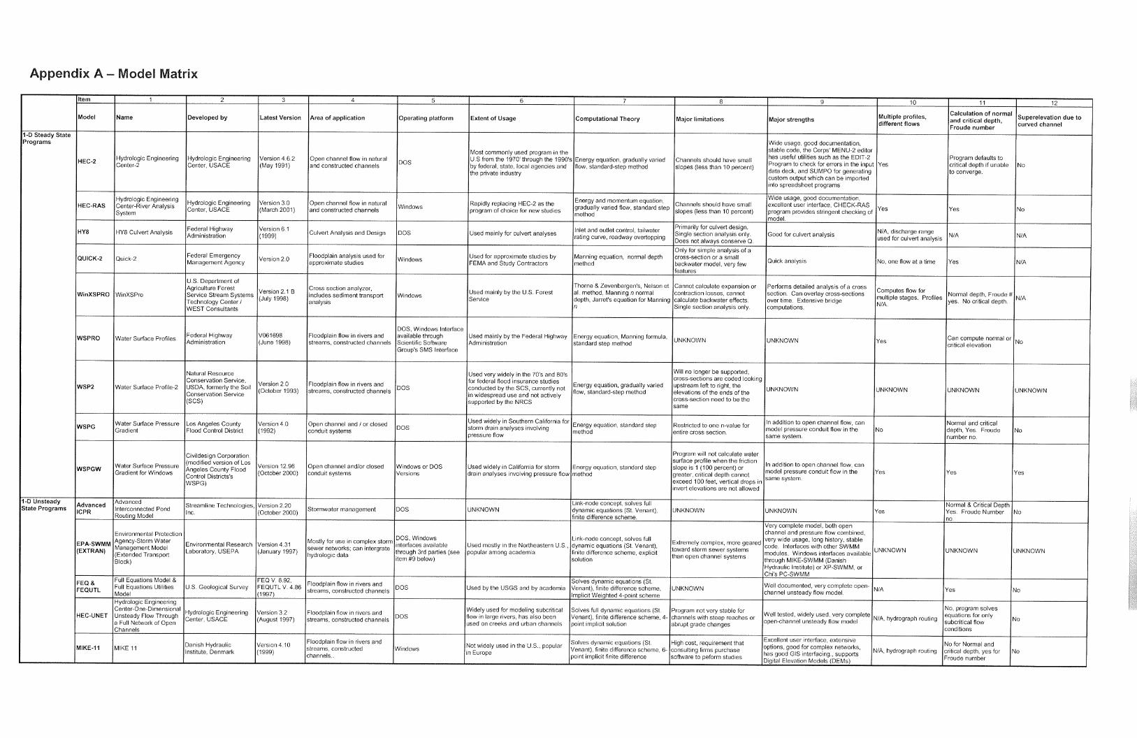
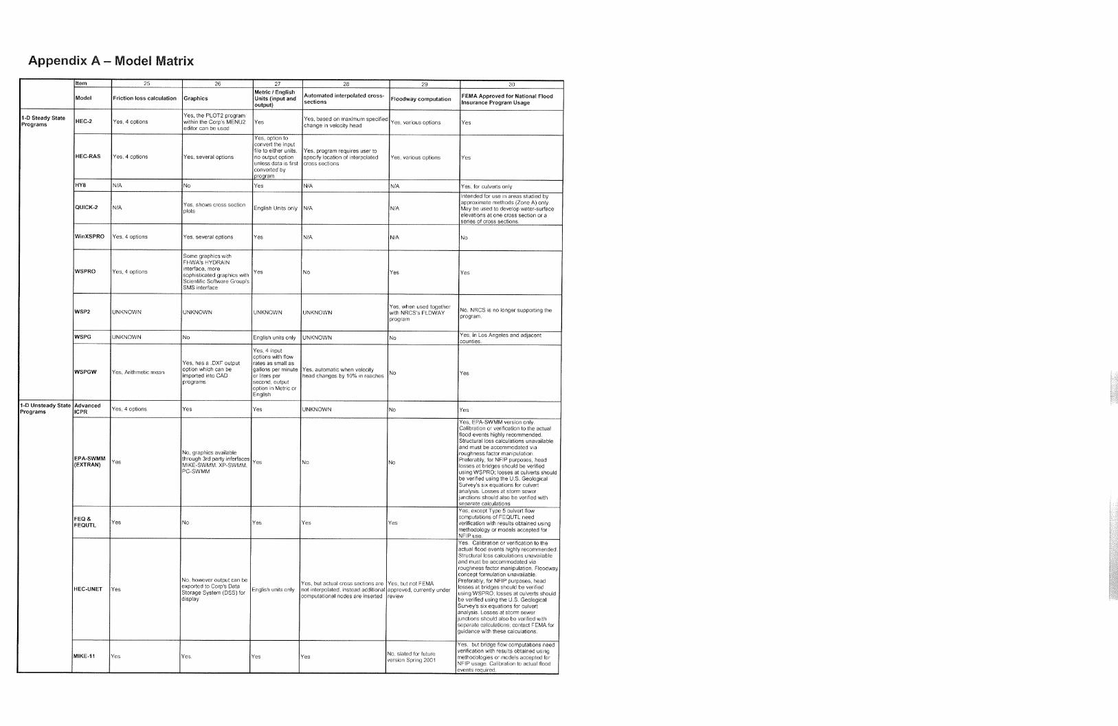
SSA9-02 July 200246

Appendix B – Hydraulic Models Accepted by FEMA for NFIP Usage(Nationally Accepted Models - shown in descending order of approximate usage)

Effective: January 11, 2002

TYPE PROGRAM DEVELOPEDBY AVAILABLE FROM COMMENTS

Hydraulic Models: Determination of Water-Surface Elevations for Riverine AnalysisHEC-RAS 2.2(September1998)

U.S. Army Corps ofEngineers

Water Resources Support CenterCorps of EngineersHydrologic Engineering Center (HEC)609 Second StreetDavis, CA 95616-4687http://www.hec.usace.army.mil/

A HEC-2 file can be imported into HEC-RAS; the usermust change the conveyance computations in HEC-RAS and make the necessary modifications to thebridge modeling before running HEC-RAS to duplicatethe results obtained using HEC-2. The use of HEC-RASfor restudying a stream previously studied using HEC-2is encouraged, as long as one of the followingconditions is met: 1) the entire stream is rerun usingHEC-RAS; or 2) the stream reach remodeled usingHEC-RAS is hydraulically independent from the rest ofthe stream. The WSPRO bridge analysis isrecommended for constricted floodplains undersubcritical flow conditions. In addition, HEC-RASversion 2.2 that performs the steady flow water-surfaceprofile calculations (SNET) has been updated to version2.2.1; it should be used for NFIP studies.

HEC-RAS 3.0.1 U.S. Army Corps ofEngineers

Water Resources Support CenterCorps of EngineersHydrologic Engineering Center609 Second StreetDavis, CA 95616-4687

Under rare circumstances, for bridges with low flow,and weir flow on the overbanks, HEC-RAS 3.0.1 maynot be able to balance the flow using weir flow equationand low flow bridge analysis methods. HEC-RAS 3.0.1will then use the energy method, and the computedenergy grade elevations and water-surface elevationsmay be on the high side.

HEC-2 4.6.22

(May 1991)US Army Corps ofEngineers

Water Resources Support Center3

Corps of EngineersHydrologic Engineering Center609 Second StreetDavis, CA 95616-4687

Includes culvert analysis and floodway options.

WSPRO(June 1988 andup)

US GeologicalSurvey,Federal HighwayAdministration(FHWA)

Federal Highway Administration(FHWA)web page at:http://www.fhwa.dot.gov/bridge/hyddescr.htm

Floodway option is available in June 1998 version. 1988version is available on the USGS web page at:http://water.usgs.gov/software/surface_water.html

FLDWY(May 1989)

US Department ofAgriculture,Natural ResourcesConservation Service

US Department of CommerceNational Technical InformationService5285 Port Royal RoadSpringfield, VA 22161

Determines the encroachment stations from equalconveyance reduction method; used in conjunction withWSP2. Encroachment stations developed using thismodel must be re-entered in WSP2 model to properlydevelop floodway.

QUICK-2 1.0and up(January 1995)

FEMA Federal Emergency ManagementAgencyHazard Identification BranchMitigation Directorate500 C Street, SWWashington, DC 20472

Intended for use in areas studied by approximatemethods (Zone A) only. May be used to develop water-surface elevations at one cross section or a series ofcross sections. May not be used to develop a floodway.

One-dimensionalSteady FlowModels

HY8 4.1 and up(November 1992)

US Department ofTransportation,Federal HighwayAdministration(FHWA)

Federal Highway Administration(FHWA)web page at:http://www.fhwa.dot.gov/bridge/hyddescr.htm

Computes water-surface elevations for flow throughmultiple parallel culverts and over the roadembankment. Software and related publication areavailable from Center for Microcomputers inTransportation (McTrans), University of Florida, 512Weil Hall, Gainesville, FL 32611-6585; and on the webat:http://www-mctrans.ce.ufl.edu/

SSA9-02 July 200247

TYPE PROGRAM DEVELOPEDBY AVAILABLE FROM COMMENTS

WSPGW 12.96(October 2000)

Los Angeles FloodControl District andJoseph E. Bonadiman& Associates, Inc.

Joseph E. Bonadiman & Associates,Inc.588 West 6th StreetSan Bernardino, CA 92410http://www.bonadiman.com

Windows version of WSPG. Computes water-surfaceprofiles and pressure gradients for open channels andclosed conduits. Can analyze multiple parallel pipes.Road overtopping cannot be computed. Open channelsare analyzed using the standard step method butroughness coefficient can not vary across the channel.Overbank analyses cannot be done. Multiple parallelpipe analysis assumes equal distribution between pipesso pipes must be of similar material, geometry, slope,and inlet configuration. Floodway function is notavailable. Demo version available from:http://www.civildesign.com

FEQ 8.92 andFEQUTL 4.68(1997, both)

Delbert D. Franz,Linsley, KraegerAssociates; andCharles S. Melching,USGS

US Geological Survey221 North Broadway AvenueUrbana, IL 61801http://water.usgs.gov/software/feq.htmland technical support available athttp://www-il.usgs.gov/proj/feq/

The FEQ model is a computer program for the solutionof full, dynamic equations of motion for one-dimensionalunsteady flow in open channels and control structures.The hydraulic characteristics for the floodplain(including the channel, overbanks, and all controlstructures affecting the movement of flow) arecomputed by its companion program FEQUTL and usedby the FEQ program. Calibration or verification to theactual flood events highly recommended. Type 5 culvertflow computations of FEQUTL need verification withresults obtained using methodology or models acceptedfor NFIP use. Floodway concept formulation isunavailable.

Advanced ICPR2.20 (October2000)

StreamlineTechnologies, Inc.

Streamline Technologies, Inc.6961 University BoulevardWinter Park, FL 32792

Previous versions of the model are not acceptable.Calibration or verification to the actual flood eventshighly recommended. Floodway concept formulationunavailable.

SWMM 4.30(May 1994), and4.31 (January1997)

US EnvironmentalProtection Agencyand Oregon StateUniversity

Center for Exposure AssessmentModelingUS Environmental Protection AgencyOffice of Research and DevelopmentEnvironmental Research Laboratory960 College Station RoadAthens, GA 30605-2720http://www.epa.gov/ceampubl/softwdos.htm

Department of Civil, Construction,and Environmental EngineeringOregon State University202 Apperson HallCorvallis, OR 97331-2302http://www.ccee.orst.edu/swmm/ftp://ftp.engr.orst.edu/pub/swmm/pc

Calibration or verification to the actual flood eventshighly recommended. Structural loss calculationsunavailable and must be accommodated via roughnessfactor manipulation. Floodway concept formulationunavailable. Preferably, for NFIP purposes, head lossesat bridges should be verified using WSPRO; losses atculverts should be verified using the US GeologicalSurvey's six equations for culvert analysis. Losses atstorm sewer junctions should also be verified withseparate calculations; contact FEMA for guidance withthese calculations. Supporting documentation forfloodway calculations is available at:http://www.fema.gov/mit/tsd/dl_swmm.htm.

UNET 4.0(April 2001)

US Army Corps ofEngineers

Water Resources Support CenterCorps of EngineersHydrologic Engineering Center (HEC)609 Second StreetDavis, CA 95616-4687

Calibration or verification to the actual flood eventshighly recommended. Comparison of bridge and culvertmodeling to other numerical models reveals significantdifferences in results; these differences may beinvestigated in the near future. Floodway optioncurrently under review, not accepted for NFIP usage.

One-dimensionalUnsteady FlowModels

FLDWAV(November 1998)

National WeatherService

Hydrologic Research LaboratoryOffice of HydrologyNational Weather Service, NOAA1345 East-West HighwaySilver Spring, MD 20910

Includes all the features of DAMBRK and DWOPERplus additional capabilities. It is a computer program forthe solution of the fully dynamic equations of motion forone-dimensional flow in open channels and controlstructures. Floodway concept formulation isunavailable. Calibration to actual flood events required.This model has the capability to model sedimenttransport. Program is supported by NWS. Supportingdocumentation is available at:http://www.fema.gov/mit/tsd/dl_fdwv.htm

SSA9-02 July 200248

TYPE PROGRAM DEVELOPEDBY AVAILABLE FROM COMMENTS

MIKE 11 HD(June 1999)

DHI Water andEnvironment

DHI Inc.Eight Neshaminy InterplexSuite 219Trevose, PA 19053

Hydrodynamic model for the solution of the fullydynamic equations of motion for one-dimensional flowin open channels and control structures. The floodplaincan be modeled separately from the main channel.Bridge flow computations need verification with resultsobtained using methodologies or models accepted forNFIP usage. Calibration to actual flood events required.Floodway concept formulation is unavailable. Thismodel has the capability to model sediment transport.The web page is at: http://www.dhi.dk

FLO-2D v.2000.11(December 2000)

Jimmy S. O'Brien,Ph.D., P.E.

FLO-2D Software, Inc.Tetra Tech, ISGP.O. Box 66Nutrioso, AZ 85932

Hydrodynamic model for the solution of the fullydynamic equations of motion for one-dimensional flowin open channels and two-dimensional flow in thefloodplain. Bridge or culvert computations must beaccomplished external to FLO-2D using methodologiesor models accepted for NFIP usage. Calibration toactual flood events required. Floodway computation isunavailable.

TABSRMA2 v. 4.3(October 1996)RMA4 v. 4.5(July 2000)

US Army Corps ofEngineers

Coastal Engineering Research CenterDepartment of the ArmyWaterways Experiment StationCorps of Engineers3909 Halls Ferry RoadVicksburg, MS 39180-6199

Limitations on split flows. Floodway concept formulationunavailable. More review anticipated for treatment ofstructures.

FESWMS 2DH1.1 and up(June 1995)

US Geological Survey US Geological SurveyNational Center12201 Sunrise Valley DriveReston, VA 22092http://water.usgs.gov/software/surface_water.html

Region 10 has conducted study in Oregon. Floodwayconcept formulation unavailable. This model has thecapability to model sediment transport.

Two-dimensionalSteady/UnsteadyFlow Models

FLO-2D v.2000.11(December 2000)

Jimmy S. O'Brien,Ph.D., P.E.

FLO-2D Software, Inc.Tetra Tech, ISGP.O. Box 66Nutrioso, AZ 85932

Hydrodynamic model that has the capabilities ofmodeling unconfined flows, complex channels,sediment transport, and mud and debris flows. It can beused for alluvial fan modeling.

SFD US Army Corps ofEngineers/FEMA

Federal Emergency ManagementAgencyHazard Identification BranchMitigation Directorate500 C Street, SWWashington, DC 20472

Simplified floodway procedure for streams with noregulatory floodway limits.

FloodwayAnalysis

PSUPRO Pennsylvania StateUniversity/US Army Corps ofEngineers/FEMA

Federal Emergency ManagementAgencyHazard Identification BranchMitigation Directorate500 C Street, SWWashington, DC 20472

Encroachment analysis for streams with no regulatoryfloodway limits.

2The enhancement of these programs in editing and graphical presentation can be obtained from severalprivate companies.3Program is typically distributed by vendors and may not be available through HEC. A list of vendors maybe obtained through HEC.

SSA9-02 July 200249

Appendix C – HEC-RAS Reviewer’s Checklist

INPUT CHECKLIST

1. GEOMETRIC DATA

A. Review the project limits (limits of data collection). Is enough information (crosssections) gathered both upstream of and downstream of the study reach? Forsubcritical regime, make sure that the upstream project limit is at a distance wherethe water surface profile resulting from a channel modification converges with theexisting conditions profile (to evaluate any upstream impacts due to projectalternatives). The downstream limit should be far enough to prevent any user-defined boundary condition from affecting the results within the study reach. Forsupercritical regime, the roles of the upstream and downstream project limits arereversed.

B. Check the river system schematic. Are the various river reaches (for a dendriticriver system) properly connected? Inspect the location of junctions. Are theflow directions correct? Check the location of flow splits and flow combinationsin looped networks (if any).

C. Review the cross section geometry. Does it characterize locations of changes indischarge, slope, shape or roughness; locations where levees begin or end, atbridges, culverts, weirs or other control structures? Are the cross sectionsproperly oriented (perpendicular to the anticipated flow lines, i.e. approximatelyperpendicular to the ground contour lines)? Review individual cross-section plots.Does a cross section extend across the entire floodplain? Is each end of the crosssection higher than the anticipated maximum water surface elevation? Is thetopography of the channel (bank stations) and floodplain accurately reflected inthe geometry of the cross sections?

D. Review the reach lengths (distances between cross sections). Check if thechannel reach lengths are correctly determined along the thalweg and theoverbank reach lengths measured along the anticipated path of the center of massof the overbank flow. Make sure that the cross section spacing properly reflectsthe stream size (? 5 times channel width), slope, uniformity of cross-section shapeand the purpose of the study.

E. Review the profile plots of channel bed elevations and top of bank elevations forabrupt changes, adverse grade or other anomalies.

SSA9-02 July 200250

2. FLOW DATA

A What is the design discharge and how is it derived?

B Is there existing discharge data (hydrologic record) that may be more appropriateor required for regulatory purposes?

C Are there any tributaries at which a change in discharge might be expected?

D Are there multiple discharges (multiple profile run)? What return interval (event)does each discharge represent?

E What is the expected flow regime? Is there a possibility for mixed flow regime?

3. BOUNDARY CONDITIONS

A. What method is used to establish the starting water surface elevation: observed,slope-area, critical or other? Is this method appropriate based on availableinformation on flow regime and topography (for subcritical flow, boundaryconditions are necessary at the downstream project limit; for supercritical flow,boundary conditions are necessary at the upstream project limit; for mixed flow,boundary conditions are necessary at both project limits)?

B. If there is not a known starting water surface elevation, prepare a range of user-defined starting elevations to check the sensitivity of the results in the study reach.

4. ENERGY LOSS COEFFICIENTS

A. What Manning's roughness coefficients are used for the channel and overbankareas? Review available aerial and/or ground photography. Conduct a fieldreconnaissance. Are the coefficients realistic and representative of vegetation,seasonal change, channel irregularities, channel alignment, channel slope, stageand discharge, and bedforms? Is there a need to model more than three distinctzones within each cross section (left overbank, channel and right overbank)?Does aerial photography or field review indicate braided channels or other areaswith the horizontal variability of roughness? Check if the observed water surfaceprofile information (gaged data and high water marks) is available for theroughness calibration. Compare the adopted Manning coefficients to those usedin other studies for similar stream conditions and/or those obtained fromexperimental data.

B. What expansion and contraction coefficients are used to evaluate transitionlosses? Are they representative of the changes in geometry between successivecross sections and flow regime? Do they include energy losses at bridges,culverts, weirs and other control structures? Make sure that the coefficients

SSA9-02 July 200251

applied between two cross sections are specified as part of the data for theupstream cross section.

5. INEFFECTIVE FLOW AREAS

A. Are non-conveying, flow separation areas where the velocity in the downstreamdirection is close to zero (e.g. "shadow" areas outside the main flow conveyancezone approaching or exiting a bridge, culvert or other flow obstacle) modeled asineffective?

B. Are depressions such as overbank excavations or low grounds where water pondsbut is not actively being conveyed, represented as ineffective flow areas?

6. SPECIAL CONDITIONS

Based on review of the input data, note the existence or any indication of the possibleexistence of the following conditions for further investigation after reviewing the output:

A. Bridges, culverts, weirs and other control structures

B. Levees

C. Blocked obstructions

D. Distributary or alluvial fan conditions

E. Split and/or divided flow

F. Islands

OUTPUT CHECKLIST

1. KEY HYDRAULIC PARAMETERS

Check the following parameters for consistency and reasonableness:

A. Flow depth

B. Critical flow depth

C. Velocity

D. Velocity head

SSA9-02 July 200252

E. Area

F. Top width

G. Invert slope

H. Energy slope

These parameters should vary gradually between successive cross sections. Note anyunusual variations and any extreme values that do not seem realistic or are inconsistent withknown conditions regarding the stream reach.

2. FLOW CONSISTENCY

A Check the streamwise variation (from cross section to cross section) in the flowdistribution between the channel and the left/right overbank. Does the amount offlow (discharge) in any one area vary dramatically from one cross section to thenext?

B Check the lateral distribution of flow between the channel and the overbanks foreach cross section. Does it seem reasonable (e.g. if majority of flow is in oneoverbank, is this what is expected based on the input review)?

3. ERROR AND WARNING MESSAGES

Review summary of errors, warnings and notes generated after each run. It is important tonote that the user does not have to eliminate all the warning messages. However, it is up tothe user to determine whether or not these warnings require additional action for the analysis.

Some common messages to look for include:

A. If there are consistent warning messages indicating profile defaulting to criticaldepth, consider modeling the alternative flow regime (subcritical vs.supercritical). Mixed flow regime should also be attempted.

B. Each cross section with the energy equation could not be balanced message (sothat critical depth was assumed), requires further examination. This message isoften an indication of unstable modeling (due to insufficient number of crosssections and data points, inconsistent flows, inaccuracy of roughness coefficientsand energy losses), rather than critical flow depths. However, it is up to the userto determine whether critical depth is a legitimate answer which indicatesminimum specific energy of the flow (e.g. at a transition from subcritical tosupercritical flow, at a sudden constriction in subcritical flow, etc.).

C. If there are any extended cross section messages (these messages indicate thecomputed vertical floodplain limits exceed the limits of the cross section),

SSA9-02 July 200253

consider obtaining additional ground points from the available topography to"close" the cross section and account for the additional flow area. Consider ifflow would actually leave the main channel at this location (split flow situation).

D. In case of divided flow messages, it should be first determined whether the watercan actually flow on both sides of the dividing land feature at the specified flowrate. If so, this usually requires separate modeling of divided reaches.

E. Messages indicating change in velocity head and/or conveyance ratio exceedingallowable limit imply that the flow areas are changing abruptly between crosssections and may call for additional cross sections or specification of ineffectiveflow limits.

F. Any other messages should be examined and either eliminated or justified.

4. SPECIAL CONDITIONS

Based on the foregoing review, determine whether the model input or output suggests any ofthe following special flow conditions:

A. Bridges and/or culverts? Are boundary cross sections properly located? Has thecorrect computational method been used (energy, momentum, Yarnell, pressureand/or weir)? Are ineffective flow limits properly specified? Check thepressure/low flow distribution in the output.

B. Levees? Is flow confined within levees allowing overbank flow only above thelevee crest stage?

C. Blocked obstructions? Note that these elements decrease flow area and addwetted perimeter when the water comes in contact with them (unlike theineffective flow limits).

D. Distributary or alluvial fan conditions? Does the output indicate consistentoccurrence of flows diverging from a common path without rejoining downstreamor do flow characteristics indicate a gradually expanding pattern of flow with littleor no boundary definition? If so, a distributary type flow pattern maypredominate, making one-dimensional modeling impractical or impossible.

E. Split and/or divided flow? Flow overtopping a divide as side weir flow? Havethese areas been accounted for using split flow modeling or other approximationto account for lost flow?

F. Islands? Do the model results indicate isolated flood free areas within thefloodplain? The occurrence of islands may indicate a flow pattern similar to splitor divided flow where the two (or more) separate flow paths around the islandmust be modeled separately to accurately determine flow profiles.

SSA9-02 July 200254