Aerosol Characterization and Analytical Modeling of Concentric Pneumatic and Flow Focusing Nebulizers for Sample Introduction

by

Arash Kashani

A thesis submitted in conformity with the requirements for the degree of PhD

Mechanical and Industrial Engineering Department University of Toronto

© Copyright by Arash Kashani, 2010

ii

Aerosol Characterization and Analytical Modeling of Concentric

Pneumatic and Flow Focusing Nebulizers for Sample Introduction

Arash Kashani

PhD

Mechanical and Industrial Engineering Department

University of Toronto

2010

Abstract

A concentric pneumatic nebulizer (CPN) and a custom designed flow focusing nebulizer (FFN)

are characterized. As will be shown, the classical Nukiyama-Tanasawa and Rizk-Lefebvre

models lead to erroneous size prediction for the concentric nebulizer under typical operating

conditions due to its specific design, geometry, dimension and different flow regimes. The

models are then modified to improve the agreement with the experimental results. The size

prediction of the modified models together with the spray velocity characterization are used to

determine the overall nebulizer efficiency and also employed as input to a new Maximum

Entropy Principle (MEP) based model to predict joint size-velocity distribution analytically. The

new MEP model is exploited to study the local variation of size-velocity distribution in contrast

to the classical models where MEP is applied globally to the entire spray cross section. As will

be demonstrated, the velocity distribution of the classical MEP models shows poor agreement

with experiments for the cases under study. Modifications to the original MEP modeling are

proposed to overcome this deficiency. In addition, the new joint size-velocity distribution agrees

better with our general understanding of the drag law and yields realistic results.

iii

Acknowledgments

I am deeply grateful to my supervisor, Professor Mostaghmi for his five years of invaluable

guidance, encouragement, support and also for giving me the luxury of experimenting and doing

the project my way. I would also like to thank Professor Coyle for attending my PhD defense and

his careful review of my work. I owe my supervising committee, Professors Sullivan, Chandra

and Ashgriz for their continued support and insightful comments. My special thanks goes to

Professor Ashgriz and his graduate student, Amirreza Amighi, who kindly let us use their lab

facilities and assisted me with the experimental part of the project. I appreciate Professor

Tanner’s group from the chemical department, particularly Mr. Vorobiev for designing the

nebulizer prototypes and Dr. Bandura for reviewing my papers, his great vision and involvement

in the project.

I am thankful to my colleagues at the Centre for Advanced Coating Technologies (CACT),

especially Dr. Hanif Montazeri for his exceptional talent and our fruitful discussion along the

way. I also owe Dr. Ala Moradian. His experience and emotional support helped me during the

tough days. I was lucky to have the company of two great friends, Araz Sarchami and Babak

Samareh in the past years.

The understanding, hard work and support of my beloved wife, Zhinous, and my great parents

made this journey possible for me. To each of them I am sincerely thankful.

iv

To my dearests, Zhinous

my mom and dad.

v

Table of Contents

Contents

Acknowledgments .......................................................................................................................... iii

Table of Contents ............................................................................................................................ v

List of Tables ................................................................................................................................ vii

List of Figures .............................................................................................................................. viii

List of Appendices ........................................................................................................................ xii

Chapter 1 Introduction .................................................................................................................... 1

1.1 Overview of components and processes in ICP-MS ........................................................... 1

1.2 Sample introduction in ICP-MS .......................................................................................... 3

1.3 Concentric Pneumatic Nebulizer (CPN) – Design and Fundamentals ............................... 5

1.4 Microsample Introduction ................................................................................................. 12

1.5 Objectives ......................................................................................................................... 19

1.6 Summary ........................................................................................................................... 20

Chapter 2 Aerosol Size Characterization of Concentric Pneumatic Nebulizer ............................ 22

2.1 Experiment Setup .............................................................................................................. 22

2.2 Nukiyama–Tanasawa Correlation ..................................................................................... 24

2.3 Rizk–Lefebvre Correlation ............................................................................................... 43

2.4 Variation of Characteristic Mean Drop Sizes ................................................................... 51

2.5 Nebulization Efficiency .................................................................................................... 55

2.6 Contribution ...................................................................................................................... 57

Chapter 3 Aerosol Size Characterization of Flow Focusing Nebulizer ........................................ 59

3.1 Nozzle Design ................................................................................................................... 59

3.2 Theoretical Background .................................................................................................... 63

vi

3.3 Droplet Size Modeling and Variation of Characteristic Mean Drop Sizes ....................... 70

3.4 Nebulizer Performance ..................................................................................................... 76

3.5 Contribution ...................................................................................................................... 83

Chapter 4 Aerosol Velocity Characterization ............................................................................... 85

4.1 General Considerations ..................................................................................................... 85

4.2 Aerosol Velocity Modeling ............................................................................................... 92

4.3 Contribution ...................................................................................................................... 98

Chapter 5 Maximum Entropy Principle - Application on Aerosol Size and Velocity Modeling . 99

5.1 The Need for Statistical Measures and Maximum Entropy Principle .............................. 99

5.2 MEP Formulation ............................................................................................................ 101

5.3 Number or Volume Based Probability Distribution Function? ...................................... 104

5.4 Global and Local Implementation of MEP ..................................................................... 110

5.5 Numerical Solution ......................................................................................................... 113

5.6 MEP Results and Discussion .......................................................................................... 115

5.7 Contribution .................................................................................................................... 127

Chapter 6 Concluding Remarks and Future Works .................................................................... 129

6.1 Contribution .................................................................................................................... 129

6.2 Future Works .................................................................................................................. 131

References ................................................................................................................................... 133

Appendices .................................................................................................................................. 146

vii

List of Tables

Table 1-1: Critical dimensions of different nebulizers used in ICP-MS, * Pressures required to

reach 0.25 and 0.6 (l/min) gas flow rates respectively. ................................................................. 14

Table 2-1: Operating conditions for nebulizers and the measurement devices exploited in

experiments ................................................................................................................................... 25

Table 2-2: Coefficients and exponent of original NT, modified NT and the fitted NT models. .. 38

Table 2-3: Comparison between the model (NT, FNT) and experimental values of D32 (µm). ... 44

Table 2-4: Coefficients and exponents of different RL type correlations, RL=original Rizk-

Lefebvre model, MRL-G=Gras’ modified model, MRL-K= Kahen et al.’s modified model,

FRL= present fitted RL model ...................................................................................................... 48

viii

List of Figures

Figure 1-1: Schematic major components in ICP-MS: i- Sample introduction system ii- Plasma

and iii- Mass Spectrometer. ............................................................................................................ 2

Figure 1-2: (a) A conventional CPN with its critical dimensions and (b) a view of nebulizer tip

under microscope, model: Meinhard TR30-C3. ............................................................................. 7

Figure 1-3: Different design and nebulizer tip of Meinhard concentric pneumatic nebulizers,

(Courtesy of Meinhard Glass Products). ......................................................................................... 8

Figure 1-4: Schematic of processes taking place at the exit of CPN. ........................................... 11

Figure 1-5: Successive stages in an idealized sheet Breakup ....................................................... 11

Figure 1-6: Close view of micronebulizer tip, (a) HEN, (b) MMN, (c) MCN and (d) conventional

CPN ............................................................................................................................................... 16

Figure 1-7: Schematic design of DIHEN and its coupling with plasma torch, (35). .................... 18

Figure 2-1: Experiment setup, dashed line represents makeup gas line and is only used for FFN.

....................................................................................................................................................... 26

Figure 2-2: Schematic of PDPA and fiber optics. ......................................................................... 27

Figure 2-3: Sauter mean diameter versus gas flow rate for distilled water and methanol from

experiment and the original NT model at (a) Ql=1 (µl/s), (b) Ql=5 (µl/s) and (c) Ql=10 (µl/s). . 32

Figure 2-4: Error between experiment and the original NT model grows larger by increasing the

liquid flow rate for (a) distilled water and (b) methanol. .............................................................. 33

Figure 2-5: Contribution of first and second term in Nukiyama – Tanasawa equation. Δ: Ql=1

(µl/s), ○: Ql=5 (µl/s) and ◊: Ql=10 (µl/s). Dashed and solid lines represent first and second term

of Nukiyama - Tanasawa equation respectively. .......................................................................... 34

Figure 2-6: Typical size distribution with TR30-C3 CPN at Ql=5 (µl/s) and Qg= 500 (sccm),

liquid: distilled water. D32=20.8 (µm), Dpeak=9.4 (µm). ............................................................... 37

ix

Figure 2-7: Sauter mean diameter versus gas flow rate from experiment, original NT model and

Kahen et al’s MNT model for distilled water at Ql=10 (µl/s). ..................................................... 39

Figure 2-8: Sauter mean diameter versus gas flow rate for distilled water and methanol from

experiment and the FNT model at (a) Ql=1 (µl/s), (b) Ql=5 (µl/s) and (c) Ql=10 (µl/s). ............ 41

Figure 2-9: Ratio of calculated to measured Sauter mean diameter versus gas flow rate for

distilled water. ............................................................................................................................... 42

Figure 2-10: Measured versus calculated Sauter mean diameter from the original NT and fitted

NT (FNT) models. ........................................................................................................................ 43

Figure 2-11: Sauter mean diameter versus gas flow rate for distilled water from experiment and

different RL type models at (a) Ql=1 (µl/s), (b) Ql=5 (µl/s) and (c) Ql=10 (µl/s). ...................... 50

Figure 2-12: Variation of (a) D30/D32 and (b) D30/D-10 versus the normalized gas low rates at the

downstream axial location of z=10 (mm). .................................................................................... 53

Figure 2-13: Variation of characteristic moment ratio with axial location (a) D30/D-10 and (b)

D30/D32 at Ql=5 (μl/s). ................................................................................................................... 54

Figure 2-14: Nebulization efficiency versus gas flow rates for distilled water measure at z=10

(mm). ............................................................................................................................................. 57

Figure 3-1: Schematic design of the first FFN. ............................................................................ 60

Figure 3-2: The actual prototype of the first custom designed FFN. ............................................ 62

Figure 3-3: Schematic design of the second FFN. ........................................................................ 63

Figure 3-4: Figure 18- Photographs taken from inside and outside of FFN (40) showing (a)-

Capillary and liquid filament, (b)-The liquid jet exiting the orifice and (c)- Unstable wave growth

on the filament surface, breakup and droplet generation .............................................................. 64

Figure 3-5: View of orifice hole and the emitted micro jet of the first FFN prototype. Orifice

diameter do=150 (µm), ΔPg=70 (Kpag) and Ql=1.66 (µl/s). Predicted jet diameter dj= 13.4 (µm).

....................................................................................................................................................... 68

x

Figure 3-6: Distribution curves for flow conditions given in Figure 3-5 (a) number and volume

distribution. (b) cumulative number and volume distribution. ..................................................... 69

Figure 3-7: Comparison between drop size models and experiments at different liquid flow rates

for FFN at: (a) 0.1, (b) 0.2, (c) 0.4, (d) 0.6 and (e) 1.0 (µl/s). ..................................................... 74

Figure 3-8: Variation of (a) D30/D32 and (b) D30/D-10 versus the normalized gas low rates at the

downstream axial location of z=10 (mm). .................................................................................... 75

Figure 3-9: Variation of characteristic moments of the primary size distribution with the jet based

Weber number meared at z=10 (mm). .......................................................................................... 77

Figure 3-10: Standard deviation of the primary size distribution of the FFN versus the jet based

Weber number measured at z=10 (mm). ....................................................................................... 78

Figure 3-11: (a) Number and volume-based size distribution and (b) Cumulative size and volume

distribution at Ql=0.2 (µl/s), Qg= 150 (milt/min), D10/dj=2.26 and Wedj=4.5, (point 1 of Figure 3-

9). .................................................................................................................................................. 80

Figure 3-12: (a) Number and volume-based size distribution and (b) Cumulative size and volume

distribution at Ql=0.6 (µl/s), Qg= 180 (milt/min), D10/dj=1.5 and Wedj=9.6 (point 2 of Figure 3-

9). .................................................................................................................................................. 81

Figure 3-13: (a) Number and volume-based size distribution and (b) Cumulative size and volume

distribution at Ql=1.0 (µl/s), Qg= 320 (ml/min), D10/dj=0.69 and Wedj=20.0 (point 3 of Figure 3-

9). .................................................................................................................................................. 82

Figure 3-14: Comparison between FFN and CPN running at comparable flow conditions Ql=1.0

(μl/s) and Qg~320-370 (ml/min). ................................................................................................... 83

Figure 4-1: Gas in a free turbulent jet exiting a 260 (µm) nebulizer operating at sonic flow and

droplet velocity for 1, 10, 20, 50 and 100 (µm) droplet diameter. ................................................ 91

Figure 4-2: Droplet Mean and Root Mean Square (rms) speed and unseeded gas velocity versus

gas flow rate, measured at z=10 (mm) for (a) CPN and (b) FFN. ................................................ 95

Figure 4-3: Span of (a) velocity and (b) size distribution measured at z=10 (mm) for CPN. ....... 96

xi

Figure 4-4: Span of (a) velocity and (b) size distribution measured at z=10 (mm) for FFN. ....... 97

Figure 5-1: Size and velocity space and probability distribution function of aerosol ................ 102

Figure 5-2: Sellens and Brzustowski’s control volume for MEP modeling. .............................. 106

Figure 5-3: Li and Tankin’s control volume for MEP modeling. ............................................... 110

Figure 5-4: Primary aerosol size distribution measured at z=10 (mm) for (a) Ql=5 (µl/s) at

Qg=500 (ml/min), D30=16.2 (µm) and (b) Ql=0.1 (µl/s) at Qg=150 (ml/min), D30=14.4 (µm).

Error bars represent standard deviation.. .................................................................................... 117

Figure 5-5: Primary aerosol velocity distribution measured at z=10 (mm) for (a) Ql=5 (µl/s) at

Qg=500 (ml/min), Uref=47.2 (m/s) and (b) Ql=0.1 (µl/s) at Qg=150 (ml/min), Uref=17.6 (m/s).

Error bars represent standard deviation.. .................................................................................... 121

Figure 5-6: Mean velocity versus droplet diameter measured at z=10 (mm) for (a) Ql=5 (µl/s) at

Qg=500 (ml/min and (b) Ql=0.1 (µl/s) at Qg=150 (ml/min), Error bars represent standard

deviation.. .................................................................................................................................... 124

Figure 5-7: Root mean square velocity versus droplet diameter measured at z=10 (mm) for (a)

Ql=5 (µl/s) at Qg=500 (ml/min) and (b) Ql=0.1 (µl/s) at Qg=150 (ml/min), Error bars represent

standard deviation. ...................................................................................................................... 126

xii

List of Appendices

Appendix A: Generation of Ripples by Wind Blowing over a Viscous Fluid…………………146

Appendix B: PDPA Calibration and Measurement…………………………………….………148

Appendix C: Axial and Radial Variation of D30/D32 and D30/D-10 Ratios of the FFN…………153

Appendix D: Spatial Variation of Mean Droplet Velocity Moments………………………..…161

Appendix E: Empirical Probability Distribution Functions ...…………………………………165

Appendix F: Derivation of Shannon entropy ………………………………………………….169

Appendix G: Bayesian and Shannon entropy …………………………………………………172

1

Chapter 1 Introduction

Overview of components and processes in ICP-MS 1.1

Radio frequency (RF) inductively coupled plasma (ICP) discharges are commonly used as

excitation and ionization sources in atomic spectrometry. Inductively Coupled Plasma Mass

Spectrometry (ICP-MS) is a well established method of trace and ultra-trace elemental and

isotopic analysis (1) and is extensively covered in the literature (2).

A typical ICP-MS device is composed of three major parts (i) Sample Introduction system, (ii)

Plasma and (iii) Mass Spectrometer as shown in Figure 1-1. First an analytical ICP is formed in a

stream of gas flowing through an assembly of three concentric quartz tubes (outer tube, inner

tube and injector tube) known as the plasma torch (3). An induction coil placed around the

plasma torch is initially triggered by an ignition circuit and forms a radio-frequency

electromagnetic field. The electromagnetic field in turn accelerates electrons and transfers energy

from the coil to the plasma in inelastic collisions with gas atoms. The physical properties of the

plasma such as ionization energy and thermal conductivity strongly depend upon the carrier gas

(4). Rare gases are usually used to generate plasma because they emit only atomic spectra in

emission spectrometry and relatively simple spectra in mass spectrometry. Among rare gases, Ar

is generally preferable due to its availability, low cost and higher kinetic energy in contrast to He

and Ne, however its low thermal conductivity (in comparison to the other two) requires a larger

sample residence time in the plasma (4).

Modern ICP-MS instruments typically operate at 1.5-2 (kW) with frequencies of 27 or 40 (MHz)

to generate gas kinetic temperature of 4000-7000 (K) and 0.1 percent ionization degree for

Argon. These large temperatures would increase the number of free electrons and also the

viscosity up to a factor of 10 for Ar in comparison to the room condition. The increasing viscous

effects would normally resist the sample introduction into the plasma. However due to the skin

effect phenomenon in the HF (high frequency) field, the energy is mainly deposited at the

periphery of the plasma, i.e. temperature and viscosity are lower along the axis of the plasma.

2

Hence the central-axial zone of the plasma facilitates sample introduction through penetration of

a carrier gas having a sufficient speed. The skin effect phenomenon explains the success of ICP

over other forms of plasmas such as microwave-induced plasma or direct-current plasma (4). As

proven the skin depth, that is the penetration of the energy at the periphery of plasma, and

coupling efficiency, which relates to the ratio of the torch radius to the skin depth is determined

by the operating frequencies (5). It has been claimed that the radio frequency of 40 (MHz) leads

to lower electron number density and gas kinetic temperature at the axis which as a result

facilitates the sample introduction (6), (7) and (8). To have an efficient spectral analysis, the

liquid sample must be completely desolvated, vaporized, atomized and ionized in the ICP torch

before entering the mass spectrometer of Figure 1-1. This is usually achieved by increasing the

surface area of the liquid sample, i.e. an aerosol is formed to enhance the rate of heat and mass

transfer. Although there are several methods for aerosol formation, pneumatic nebulization to

this day is the most widely used method for sample introduction in ICP-MS. Since the plasma

itself is produced from the argon gas stream, it would be logical to energize and employ the same

gas stream for aerosol generation (4). This is the basis of pneumatic nebulization which will be

further discussed in the next sections.

ArICP Torch

Waste

Spray Chamber Pneumatic Nebulizer

Liquid SamplePump

Mass Spectrometer

Plasma

Sample Introduction

Figure 1-1: Schematic major components in ICP-MS: i- Sample introduction system ii- Plasma

and iii- Mass Spectrometer.

3

Sample introduction in ICP-MS 1.2

Sample Introduction in ICP-MS includes two major separate processes in general: First, aerosol

generation usually by means of pneumatic nebulization and second, aerosol modification or

filtration in a spray chamber.

Although there are a variety of pneumatic nebulizers in ICP-MS, each suitable for a particular

application, they all must meet some general requirements to produce an ideal stream of aerosol.

For instance Kahen et al. mentioned that an ideal aerosol for ICP-MS must contain small and

slow droplets with uniform size and velocity (9). In fact an ideal aerosol should contain droplets

smaller than 10 (μm) for complete desolvation (10), since large droplets are not consumable by

the plasma and may halt spectrometry by cooling a surprisingly large (1-2 mm wide) volume of

the plasma (11) whereas droplets larger than 25 (μm) are not desolvated at all. Todoli and

Mermet (4) state the ideal aerosol must also have uniform droplet number density, uniform

spatial droplet diameters and have similar characteristics irrespective of the sample composition,

i.e. the physical properties should not affect aerosol characteristics. Mclean et al. (12) also add

that the key properties of the plasma like gas temperature, electron temperature and number

density should not be altered by the aerosol. As well, the presence of the aerosol shouldn’t affect

the optimum sampling depth of ions in the analysis of different samples and furthermore the

aerosol must not contribute a solvent load to the plasma. According to the ideal aerosol

properties mentioned above and some other considerations an ideal nebulizer is defined by (12)

and (13) as a device that:

i. consumes small quantities of sample and reagents (small consumption rate),

ii. is able to nebulize wide ranges of solution,

iii. provides 100 percent transport efficiency,

iv. nebulizes solutions containing high solid concentration without clogging or premature

failure,

v. contains no dead volume,

4

vi. contributes no adverse solvent load effects,

vii. its aerosol properties can be predicted by simple models,

viii. generates fine and monodisperse droplets,

ix. creates a narrow plume,

x. is rugged, inexpensive and easy to use.

The currently available nebulizers, as will be discussed, are far from ideal. Even the most

advanced ones only address some of the aforementioned points. For instance, many of the

common pneumatic nebulizers generate relatively coarse and fast aerosol with wide size and

velocity distributions, in other words they exhibit aerosol qualities not suitable for plasma. Thus

the produced aerosols have to be modified and drops must be selectively removed in spray

chambers through a process which is highly inefficient because only 2 percent of the original

aerosol generated by conventional pneumatic nebulizers finds its way into the plasma after

filtration (13). Moreover spray chambers add more complexity to the sample introduction system

that is not desired. In some other instances, the new designs compromise between some of the

main features of the nebulizer and in some cases even sacrifice one for the others, like improving

aerosol generation by modifying nebulizer geometry at the cost of increasing the probability of

nebulizer tip clogging.

Although ICP is considered a routine and mature technique for elemental analysis, its sample

introduction system has remained the weakest point of the instrument (4). Despite the significant

number of publications on sample introduction in ICPs, the commercially available ICP-MS

systems still employ the 70’s nebulizer technology and spray chamber configuration. Todoli and

Mermet (4) attribute this trend to the fact that the majority of studies are or more or less

modifications or improvements rather than a radical step change in terms of sensitivity, precision

and non-spectral interferences. Hence the necessity of comprehensive research on the optimal

design and improvement of sample introduction components to address key problems of ideal

nebulization and spray modification is widely recognized because the future development of

ICP-MS is strongly linked to improvement of the sample introduction system. Reaching that goal

is still left a challenge for the researchers in this field.

5

Concentric Pneumatic Nebulizer (CPN) – Design and 1.3Fundamentals

Today’s modern CPN does not differ fundamentally from the nebulizer described by Gouy (14)

at the end of the 19th

century and the technique has remained the most widely used for sample

introduction in ICPs due to its reliability, robustness, ease of operation (13) and simplicity

because it has no moving or electric parts (15), besides its versatility of aerosol production

allows researchers to adapt new designs for special needs such as high dissolved solid

nebulization, micronebulization and etc. Furthermore there is no better alternative available so

far that demonstrates a better compromise between quality of the results, nebulizer robustness

and ease of operation (4). The small cost of CPN is another important factor, currently as of

March 2009, conventional CPNs are listed between 280 to 530 USD in the manufacturer’s

catalogue (16) in comparison to Direct Injection High Efficiency (DIHEN) from the same vendor

with a price range of 1600 to 5000 USD.

Figure 1-2 shows a conventional Meinhard all glass type-C concentric nebulizer (17) together

with its dimensions. As can be seen, liquid is fed horizontally from the left hand side and travels

along a capillary tube while the gas is introduced from the bottom and moves concentrically with

the liquid, nevertheless the interaction of the two phases is restricted to the area close to the tip of

the nebulizer. The Meinhard CPN has three different designs, Types A, C and K. Type A is the

first commercially available nebulizer from Meinhard and as can be seen from Figure 1-3, the

nebulizer tip and capillary are both coplanar while the capillary for types C and K is recessed.

Tip recession is specially recommended to avoid nebulizer tip blocking (18). Therefore the type

A CPN is designed for general introduction purposes while type C and K are more suitable for

introduction of high concentration solids. The tip recession can be easily recognized in Figure

1-2b where the capillary walls are defocused in contrast to the gas annulus area. The major

difference between types C and K are in the final finishing of the nebulizer tip, while type C has

a flame polish tip; type K tip surface is ground flat and square as type A (Figure 1-3).

The CPN configuration allows the liquid to be freely aspirated without any need for a delivery

device (e.g. peristaltic pumps) due to Venturi effect, it should also be added that the free

aspiration is a unique characteristics of CPNs. Based on the CPN design, type A is expected to

6

have higher suction effect due its larger pressure difference beyond the capillary because types C

and K are recessed and the gas energy and speed is higher inside than outside of the nebulizer.

However, a free uptake rate enhancement of 1.5-2 folds has been reported for the recessed

capillaries (19). All the CPNs may utilize a peristaltic pump for liquid injection at a desired rate.

Using such a device removes the effect of liquid viscosity, an important parameter in self

aspiration, but at the same time introduces periodic noise in aerosol generation due to the

pulsating nature of the pumps. It has been reported that the CPNs have their best performance if

the injection rate is close to the free liquid aspiration rate (4).

A comprehensive study of aerosol generation for CPN and ICP-MS nebulizers in general is a

difficult task because the process is rather fast and happens in a very short timescale (in the order

of several milliseconds), besides there are several fairly complicated processes involved in

droplet generation which are poorly understood. In fact most of the studies aimed at aerosol

production have been carried out in different fields of engineering and aeronautics where the

nozzles and flow conditions are not comparable to ICP-MS applications.

The pneumatic aerosol generation can be divided into two separate processes (i) wave generation

on the liquid surface and (ii) growing of instabilities and disintegration of waves to form

droplets. Under the regular conditions of nebulization in ICP-MS applications, waves with

wavelengths of the order of several tens of micrometers are formed on the liquid surface due to

transfer of energy from the gas phase. However, the gas and liquid velocity at the contact surface

is only a percent of the gas stream because only tangential velocity components are acting on the

surface; as a result a small fraction of gas energy is used for wave generation.

Once the waves are formed, the degree of interaction between the gas and liquid increases. The

magnitude of the force acting on a single wave depends on the relative velocity between the two

phases, wave dimension and drag coefficient. Note that the presence of turbulence increases the

penetration of gas in the liquid bulk and promotes wave generation and growth until the wave

becomes unstable and is fragmented into droplets (4). The wave destruction can be attributed to

three separate mechanisms (20):

1- Filament or sheet formation followed by a collapse into droplets under the combined

action of the gas and the surface tension of the liquid.

7

2- Direct boundary layer stripping of the wave crests.

3- Removal of the surface disturbances through “Taylor instabilities” (21).

The first two processes are principally derived from tangential stresses on the liquid boundary

layer and generally produce fine droplets while the Taylor instability mechanism is due to the

action of normal forces and may lead to large droplet generation, especially if the liquid feed rate

Figure 1-2: (a) A conventional CPN with its critical dimensions and (b) a view of nebulizer tip

under microscope, model: Meinhard TR30-C3.

8

exceeds the rate of liquid removal by the other two processes. It’s worth mentioning that the

surface tension forces resist surface deformation and wave disintegration; as well the liquid

viscosity strongly damps the short wavelengths. Thus low surface tension and viscosity favors

fine aerosol generation as confirmed by (12) and (20).

Figure 1-4 and Figure 1-5 exhibits the wave formation and droplet generation for CPN

schematically. As can be seen the liquid discharging from the centered capillaries is pulled

toward the gas exit due to smaller local pressure. Liquid stretching would in turn decrease the

thickness of formed film and consequently enhances the gas and liquid interaction (20). This

process is called prefilming and is in fact one of the unique features of concentric nebulizers.

Figure 1-3: Different design and nebulizer tip of Meinhard concentric pneumatic nebulizers,

(Courtesy of Meinhard Glass Products).

9

At this stage, it would be interesting to have some qualitative measure for the wavelengths

perturbing the liquid film and from there some raw estimation on the size of resulted droplets.

In reference (22), Squire studied the instability of an infinitely wide moving liquid film with

constant thickness and negligible viscosity. Although the details of his mathematical

formulation are beyond the scope of this chapter, some important conclusions may be drawn.

First the minimum wavelength for an unstable film was given as:

(1-1)

here λmin, ζ, ρg and UR are the wavelength, surface tension, gas density and relative velocity

between liquid and gas velocity respectively. Assuming argon is used close to the sonic

condition and recalling that liquid velocity is negligible compared to gas velocity, then for

UR=ug=276.1 (m/s), ρg=2.217 (kg/m3) and ζ=0.072 (N/m), λmin=2.67 (μm). Hence Equation (1-1)

suggests any wave whose wavelength is shorter than the characteristic value of 2.67 (μm), will

eventually be damped in the flow and does not contribute to the droplet generation. Furthermore,

Squire calculated the optimum wavelength (Figure 1-5) which maximizes the growth rate of

perturbations and produces the most probable drop size by:

(1-2)

Plugging the same values as in Equation (1-1), the optimum wavelength would be λopt=5.35(μm).

Knowing that the drop sizes must be of the same order of magnitude as their generating

wavelength, 5.4 (μm) is the modal characteristic length for ICP-MS nebulizers and as will be

seen in the next chapters, the most probable droplet size is in the same order as predicted by

Equation (1-2). One important feature of Equation (1-2) is its independence from the film

thickness, whilst the thickness of the prefilmed liquid of Figure 1-4 is continuously decreasing.

Rizk and Lefebvre (23) found that for all prefilming type of airblast atomizers, the thickness of

the liquid film at the atomizing jet is mainly governed by the liquid viscosity, the air velocity and

the relative mass flow rates of liquid and air. The film width is also finite and the liquid may not

necessarily have negligible viscosity which would make some deviation from our calculation.

10

Thus the Squire analysis is not intended to give exact value or model a realistic flow condition

but rather present some rough estimate of the length scales here.

Taylor (24) also investigated the problem of ripple formation induced by wind blowing over the

viscous fluid surface and expressed the optimum wavelength as a rather complicated function:

( )

(1-3)

where ηl is the liquid viscosity. Again for the same flow conditions of Equation (1-2) and the

liquid viscosity of ηl=0.001 (Pa.s), θ will be 31.4 and the corresponding wavelength would be

4.7 (μm). Refer to the Appendix A for the shape of the θ function and more details.

Finally, Merrington and Richardson (25) showed a free body of liquid is unstable for Weber

numbers (We= ρgUR2L/ζ>10) where L is a characteristic length. Substituting with appropriate

values once again a characteristic length of 4.3 (μm) is obtained. Thus the characteristic

dimension (optimum wavelength) is of the order of 4-6 (μm) for nominal ICP-MS operating

conditions, although the models (22), (24) and (25) do not necessarily represent the actual

physics of the problem.

When the high velocity gas exits the nebulizer (Figure 1-4), gas streams are entrained from both

sides of the jet due to the pressure drop. Nevertheless in the region surrounded by the high

momentum gas, the entrainment must be supplied by the trapped gas itself which would cause

the formation of toroidal shape vortices. Therefore the liquid surface at the capillary end is

spread out and forms a meniscus from which a series of ligaments as large as the capillary inner

diameter are generated and finally disintegrate into fine droplets. However the frequent

coalescence of these ligaments may promote the generation of coarse droplets that is not desired.

The two gas streams finally recombine with each other and transport the aerosol drops

downstream while normally expanding. The recombination is believed to occur at a location

about half the outer capillary diameter along the axis of the nebulizer (20).

It’s been claimed in that pneumatic aerosol generation, the liquid core is unaltered up to 5 times

the capillary diameters. For TR30-C3 CPN for example, the average capillary is about 250 (μm),

11

Figure 1-4: Schematic of processes taking place at the exit of CPN.

Figure 1-5: Successive stages in an idealized sheet Breakup

L = 5 x AA

Ligament and drop formation

Prefilming

Renublization

Toroidal gas vortex

Spray Plume

Recombination region

Gas exit

12

that would give a length of 1250 (μm) approximately. Over such distance, gas would normally

lose a great deal of its kinetic energy required for liquid breakup due to expansion and become a

source for droplet acceleration or transport. For an efficient nebulization, the gas-liquid

interaction must be as efficient as possible but as Figure 1-4 shows, only one side of the gas jet is

in direct contact with the liquid and is used for droplet production. Thus the conventional

concentric designs are not the best choice for fine aerosol production (4), (18) and (20) in ICP-

MS, hence the CPN must be coupled with aerosol modification devices, i.e. spray chambers or

desolvation systems, to remove the coarse droplets. The need for improved or alternative sample

introduction methods is clear, recalling that the combination of the CPN and spray chambers

results in very poor transport efficiency (the ratio of aerosol reaching the atomization cell to the

total mass sprayed).

Microsample Introduction 1.4

Microsample introduction in ICP-MS has been the subject of many studies in the past 15 years to

several reasons:

(i) in some particular fields (e.g., forensic, biological and clinical analysis, etc.) the available

sample volume may be significantly lower than 1 (ml). (ii) several interferences like polyatomic

ones in ICP-MS can be positively reduced when working at low liquid flow rates. (iii) toxic and

radioactive wastes must be minimized in some applications and (iv) the transport efficiency is

improved at small liquid sample consumption rates.

Conventional CPNs operate at solution feed rate on the order of 0.5-2 (ml/min), this would

require a sample volume of 1-10 (ml) for roughly 5 minutes of analysis. Recall that the

conventional CPNs are not efficient nebulizing devices and their employment for microsample

introduction requires a rather large volume of liquid which is neither always practical nor

affordable, in addition coupling CPNs with spray chambers usually results in very poor transport

efficiency. Exploiting the conventional CPNs at microsample conditions (Ql=10-300 μl/min)

may also lead to dramatic loss of sensitivity and an increase in washout times (4), besides Todoli

and Mermet (18) and Mora et al. (13) claim the critical dimensions of CPNs are not suitable

microsample introduction. As stated before the CPNs have their best performance close to the

aspiration rate; lowering the liquid feed rate below 300 (μl/min) has been reported to cause

13

unstable aerosol generation (26). In the author’s experience with Meinhard TR30-C3 CPN, a

stable aerosol was observed at a flow rate as low as 60 (μl/min).

Therefore microsample introduction requires its own micronebulizer design. In the past decade

several micronebulizers have been developed and demonstrated better performance in terms of

better aerosol generation, higher ICP sensitivities and lower limits of detection at low liquid flow

rates. The micronebulizers have more or less followed the original concentric design and the

nebulizer miniaturization is mainly done through lowering the capillary diameter, wall thickness

and in some cases by reducing the gas-exit cross sectional area. Table 1-1 (taken from (4) and

(18)) compares the critical dimensions of conventional nebulizers to some of their miniaturized

counterparts.

Note in the table, HEN, MMN, MCN, DIN, DIHEN, LB-DIHEN stand for High-Efficiency

Nebulizer, MicroMist Nebulizer, Microconcentric Nebulizer, Direct-Injection Nebulizer, Direct-

Injection High-Efficiency Nebulizer and Large Bore Direct-Injection High-Efficiency Nebulizer

respectively and PFA or PFAN is a special micronebulizer made of tetrafluoroethylene-per-

fluoroalkylvinyl ether copolymer.

Several important conclusions can be drawn from Table 1-1 that may account for better

performance of micronebulizers (18):

i. The length of unaltered liquid core is shorter for micronebulizers. As stated in section

1-3, this length is about 5 times the capillary diameter. According to Table 1-1 for a

conventional CPN, the liquid core extends approximately 2000 (μm) and around 400-

500 (μm) for HEN. Therefore liquid disintegration occurs closer to the nebulizer tip

where gas has higher kinetic energy and a finer aerosol is expected.

ii. The area of gas-liquid interaction is modified for micronebulizer. This area is defined

by multiplying the distance L, along which gas is able to generate droplets, by the the

perimeter of the sample capillary. The distance L is said to be 5 times the annulus

width of the gas exit. Thus for CPN and a 20-30 (μm) wide annulus; the length L

would be 100-150 (μm) and for a sample capillary perimeter of 1.63 (mm) the

resulting interaction area is 0.16-0.25 (mm2). Similar calculations for HEN, MCN and

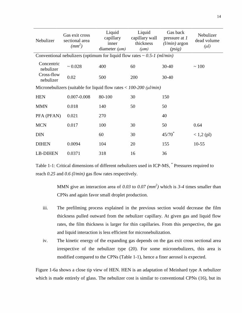
14

Nebulizer

Gas exit cross

sectional area

(mm2)

Liquid

capillary

inner

diameter (μm)

Liquid

capillary wall

thickness

(μm)

Gas back

pressure at 1

(l/min) argon

(psig)

Nebulizer

dead volume

(μl)

Conventional nebulizers (optimum for liquid flow rates ~ 0.5-1 (ml/min)

Concentric

nebulizer ~ 0.028 400 60 30-40 ~ 100

Cross-flow

nebulizer 0.02 500 200 30-40

Micronebulizers (suitable for liquid flow rates < 100-200 (μl/min)

HEN 0.007-0.008 80-100 30 150

MMN 0.018 140 50 50

PFA (PFAN) 0.021 270 40

MCN 0.017 100 30 50 0.64

DIN 60 30 45/70* < 1,2 (pl)

DIHEN 0.0094 104 20 155 10-55

LB-DIHEN 0.0371 318 16 36

Table 1-1: Critical dimensions of different nebulizers used in ICP-MS, * Pressures required to

reach 0.25 and 0.6 (l/min) gas flow rates respectively.

MMN give an interaction area of 0.03 to 0.07 (mm2) which is 3-4 times smaller than

CPNs and again favor small droplet production.

iii. The prefilming process explained in the previous section would decrease the film

thickness pulled outward from the nebulizer capillary. At given gas and liquid flow

rates, the film thickness is larger for thin capillaries. From this perspective, the gas

and liquid interaction is less efficient for micronebulization.

iv. The kinetic energy of the expanding gas depends on the gas exit cross sectional area

irrespective of the nebulizer type (20). For some micronebulizers, this area is

modified compared to the CPNs (Table 1-1), hence a finer aerosol is expected.

Figure 1-6a shows a close tip view of HEN. HEN is an adaptation of Meinhard type A nebulizer

which is made entirely of glass. The nebulizer cost is similar to conventional CPNs (16), but its

15

reduced gas exit cross sectional area requires an external additional gas cylinder and

consequently using special high pressure adapters and lines for gas streams (18). HEN is

reported to achieve transport efficiency between 90 and 95 percent for liquid flow rates of

Ql=10-1200 (μl/min) (27). The tertiary aerosol (aerosol leaving the spray chamber) of HEN and

CPN has similar velocity but the velocity distribution is considerably narrower for HEN which

leads to better ICP-MS short term signal precision (28). HEN also benefits from a similar droplet

number density for the tertiary aerosol as conventional CPN but at liquid flow rates 100 times

smaller (27). Aside from all the mentioned benefits, HEN suffers from some shortcomings. For

example, due to its small capillary diameter, tip blockage is a frequent problem and avoiding it

needs precise sample filtration even for clean aqueous solutions. In addition, HEN is a very

fragile device and may be easily broken if the nebulizer cleaning is not done carefully (26).

Furthermore the irreproducibility or variability of results is another problem that differs from one

HEN to another.

Another commercially available micronebulizer is the MicroConcentric Nebulizer (MCN) that is

made of polyamide. As can be seen from Figure 1-6c the capillary is extended outside of the

nebulizer tip that shows tolerance to high solid content solutions (29). In fact this is a drawback

for the nebulizer design since gas rapidly loses a fraction of its kinetic energy by expansion.

Besides an extended capillary may deteriorate in long term use and influence aerosol generation.

Thus MCN is considered a rather fragile nebulizer (18), but gives rise to limits of detection close

to or slightly higher than conventional CPNs operated at liquid flow rates more than 10 times

higher in ICP-AES (Inductively Coupled Plasma- Atomic Emission Spectrometry) (30) and

higher ICP-MS sensitivities.

The MicroMist Nebulizer (Figure 1-6b) is a glass modified version of common concentric

nebulizer with reduced dimensions. The major difference between MMN and other

micronebulizers is the tip recession that makes it a suitable option for introduction of high salt

content sample with peace of mind from tip blockage. The capillary inner diameter in this

nebulizer is tapered; that has probably caused the result irreproducibility between MMNs (18).

16

Since the gas exit cross sectional area is smaller for HEN, it would naturally need higher back

pressure to discharge gas at the same rate of flow. From Table 1-1, it’s noticed that the required

back pressure for injecting 1 (l/min) argon for HEN>MMN, MCN> PFA implying the kinetic

energy for aerosol generation is larger for HEN as verified by Todoli and Mermet (4) and (31).

However it should be noted again, there is currently no ultimate nebulizer for all applications.

Each nebulizer has its own advantages and drawbacks and is suited for a particular application in

sample introduction.

Although the discussed micronebulilzers (HEN, MMN, MCN and PFA) produce superior aerosol

in comparison to the conventional CPNs, they still need to be coupled with spray chambers or

desolvation systems. However these instruments are complex and have problems of their own (4)

, to name a few we can mention: (i) existence of memory effects, (ii) intensification of matrix

Figure 1-6: Close view of micronebulizer tip, (a) HEN, (b) MMN, (c) MCN and (d)

conventional CPN

17

effects, (iii) increase of signal noise, (iv) removal of a high proportion of the analyte nebulized

with subsequent loss of sensitivity, (v) wave generation and (vi) postcolumn broadening effects

when separation methods are coupled to ICP techniques.

To avoid these complexities, a new trend is observed toward total aerosol consumption and

direct injection of droplets into the plasma without exploiting spray chambers or desolvation

systems. The last 3 nebulizers in Table 1-1 are of this type. For example, excellent signal

stabilities are reported by a DIN whose capillary diameter was 60 (μm) and operated at 0.2-0.5

(l/min) argon flow and 50-100 (μl/min) liquid flow rate (32) in addition to an external 0.3 (l/min)

makeup gas flow rate to efficiently direct aerosol toward the plasma due to the low rate of the

main argon flow. Like other concentric pneumatic nebulizers, the coarse droplets of DIN are at

the periphery of the spray but the resulting primary aerosol is smaller than the CPNs because of

its reduced dimensions. However in some instances the combination of the CPN and spray

chamber is claimed to produce finer aerosol than DIN (33) but at the cost of very poor transport

efficiency, increased memory effect and poor precision.

DIN is usually placed 1 (mm) below the torch central tube which would increase the nebulizer tip

overheating especially when the HF power increases above 1.3 (kW) (34). Besides, tip blockage

is very common for this nebulizer but it can be avoided by extending the liquid capillary outside

of the nebulizer tip or increasing the make flow rate. Moreover, DIN should only be used for low

liquid flow rates and cannot be used with peristaltic pumps.

DIHEN is an all glass or quartz nebulizer by Meinhard Glass Products (17) that is a cheaper

version of DIN. The nebulizer is very close to HEN in design but about 2.5 times longer, can be

used with peristaltic pumps and is equipped by a supporting tube to reduce the capillary damage

caused by the gas stream-induced oscillations giving it high robustness (Figure 1-7, (35) and

(36)). The critical dimensions of DIHEN are smaller than DIN but may differ from one nebulizer

to another that causing irreproducibility in results. Todoli and Mermet (4) and (37) Paredes et al.

(37) believe high cost, fragility, tip blockage and overheating and the nebulizer sensitivity to

change in operating conditions and sample matrix when used in the plasma have limited the wide

application of this nebulizer for routine analysis despite its advantages. Besides the reported

analytical figures of merit obtained by DIHEN are not as good as expected for two reasons: first,

18

formation of coarse droplet as large as 30 (μm) (38) and second, the rotational motion of the

aerosol (39) which leads to aerosol deposition across the torch. Thus only 30-45 percent of the

droplets find their way into plasma without dispersion and successfully contributed to signals (4).

The tip blocking problem of DIHEN has been overcome by the new design LBDIHEN (Large

Bore DIHEN) which has enlarged capillary and gas annulus area (Table 1-1). The modified

dimensions of LBDIHEN in turn will cause larger aerosol mean diameters and small drop

Figure 1-7: Schematic design of DIHEN and its coupling with plasma torch, (35).

19

velocities, lower ICP-MS sensitivities and more severe matrix effects than DIHEN (40) but the

nebulizer is very suitable for introducing high salt content solutions and slurries.

Objectives 1.5

In this task, a type-C CPN is characterized and will be analytically modeled because not only it is

a good choice for PDPA calibration but it is also a benchmark nebulizer with wide application in

spectrometry. The aerosol size of the nebulizer is characterized in Chapter 2 and the application

of the well known Nukiyama-Tanasawa (NT) and Rizk-Lefebvre (RL) correlations are tested for

the nebulizer under the typical ICP-MS operating conditions. The aerosol velocity of the

nebulizer is then characterized in Chapter 4.

A new direct injection nebulizer will be introduced in Chapter 3 which is not of the prefilming

kind. The new custom-designed nebulizer follows the principle of Flow Focusing Nebulizer

(FFN) first employed by Ganan-Calvo (41). This new class of nebulizers is not commercially

available and has been recently employed for sample introduction in spectrometry (42) and (43) .

The preliminary results of our custom-designed nebulizer are promising although not ideal. The

author believes by resolving some issues of the FFN, it could be an alternative for many of the

current pneumatic nebulizers. The nebulizer is characterized and the fundamentals of the new

custom-designed FFN are discussed in Chapter 3 while the aerosol velocity is characterized in

Chapter 4.

Since characterization results do not represent the actual aerosol, having some statistical measure

of the aerosol is a prerequisite for any numerical or analytical modeling. Thus the other scope of

this task is to present a meaningful and detailed space of aerosol size and velocity (based on

characterization results of chapters 2, 3 and 4) from which physical size and velocity

distributions could be derived. The method of maximum entropy principle (MEP) is used for this

purpose. As will be shown in Chapter 5, the conventional MEP models yield realistic size

distribution while their velocity distribution shows poor agreement with experiments. New

modified MEP models are then proposed to overcome this deficiency and the models will be

tested for both the CPN and the FFN.

20

Summary 1.6

The maximum solvent load and acceptable gas flow rate in ICP-MS put severe constraint on

aerosol generation. For instance, droplets larger than 10 (μm) do not undergo desolvation,

vaporization and ionization processes and are not consumed by plasma. They may even cease

mass spectrometry if they constitute a large fraction of the aerosols. For ICP-MS application,

small and slow aerosol with narrow size and velocity distribution is desired, but common

concentric pneumatic nebulizer design does not fulfill these requirements and the resultant

aerosol stream is generally polydisperse with droplets sometimes as large as 100 (μm). Hence the

CPNs are usually integrated with transported instruments such as spray chambers and

desolvation systems to modify the primary aerosol generated by the nebulizer. Although spray

chamber can reduce the solvent load and remove the coarse droplets, but they add more

complexity to the sample introduction system, besides the combination of spray chambers and

CPNs leads to very poor transport efficiency between 1-2.5 percent. As proven, the critical

dimensions of CPNs such as liquid capillary diameter, wall thickness and gas exit cross sectional

area are not suitable for fine aerosol production. Therefore to improve the atomization and

overcome the low transport efficiency of spray chambers, the CPNs have been miniaturized

while keeping the same fundamentals and principals. The different micronebulizers designs

available, e.g., HEN, MMN, MCN, PFA and others that have all shown better aerosol production

by improving gas-liquid interaction area and benefiting from higher gas kinetic energy at the

nebulizer exit. Since the critical dimension, particularly liquid capillary is reduced for these

nebulizers; the tip blockage has become more problematic. The reduced dimensions also require

higher gas back pressure that needs additional pressure adapters and lines, increase the cost and

bring safety issues as well. In addition to high cost, fragility and results irreproducibility are

some other common problems associated with micro nebulizers.

Total aerosol consumption is a new trend observed for ICP-MS that is designing and employing

nebulizers that can successfully generate fine aerosol below 10 (μm) in size and directly inject

them into plasma without the need for spray chambers or desolvation systems. DIN, DIHEN and

LB-DIHEN are examples of direct injection nebulizers. Although these nebulizers are shown to

have many advantages in terms of aerosol generation and signal quality in MS, but they severely

suffer from some other drawbacks. Their cost is quite significant in comparison to conventional

21

CPNs. The positioning of the nebulizer close to the high temperature plasma often causes tip

overheating. Tip blockage is also repeatedly reported due to their reduced dimensions.

Furthermore, in the case of DIHEN, formation of droplets as large as 30 (μm) and the radial

dispersion of the aerosol increases the droplet deposition in the plasma channel and leads to

general performance not as good as expected.

In a nutshell a nebulizer able to produce fine and narrow aerosol that is not fragile, does not

require a spray chamber, can overcome tip blockage, offers result reproducibility and satisfies

signal quality at a reasonable cost is of high demand in ICP-MS.

22

Chapter 2 Aerosol Size Characterization of Concentric Pneumatic Nebulizer

Experiment Setup 2.1

A conventional TR30-C3 CPN (Figure 1-2) was selected for aerosol characterization because

Meinhard CPNs have been commercially available for a number of years, supplied as standard

ICP-MS sample introduction instruments and are often regarded as a “bench mark” nebulizer to

study sprays and also for comparison as in (33) and (44). In addition to CPN and inspired by

Ganan-Calvo’s flow focusing pneumatic nebulizer (FFPN) (41), a FFN was designed twice in

collaboration with Tanner’s group from the Department of Chemistry at the University of

Toronto (45). The initial design of the FFN was equipped with two CCD cameras to observe

filament formation inside the nebulizer and its disintegration downstream of the orifice. In the

second design, some improvements were carried out to improve nebulizer performance and the

cameras were removed from nebulizer design.

Argon was supplied to the nebulizers (both CPN and FFN) from a pressurized tank (4.8-300SZ,

Linde, Canada) while the nebulizer back pressure was regulated (5126AD, Scott Specialty

Gases, Canada). The volumetric gas flow rate was recorded with a mass flow controller and

readout placed on the gas line (MKS-Type246C, MKS Instruments, MA, USA). For the FFN, an

extra argon line (makeup flow) was used for aerosol transportation and controlled separately

with a Rotameter (PMR1-010537, Cole-Parmer Canada Inc, QC, Canada).

A 5cc-plastic (Becton Dickinson, ON, Canada) and a 1cc-glass (Hamilton Company, NV, USA)

syringe and a computer-controlled model-22 syringe pump (Harvard apparatus, MS, USA) were

exploited for sample injection. Although the C3-CPN can aspirate liquid sample freely at the rate

of 3 (ml/min) or 50 (μl/s), in the experiments the liquid was introduced manually via the syringe

pump system at the rate of 1-10 (μl/s) as in (33) to study the lower end limits of aerosol

production with this nebulizer. In this range the nebulizer is expected to generate finer aerosol

since the available gas kinetic energy per unit volume of liquid is larger than at the free

aspiration rate. Sutton et al. (26) reported unstable aerosol production for liquid flow rates below

23

Ql= 5 (μl/s), however in the author’s experiments the CPN operated robustly down to 1 (μl/s).

Any further decrease in the liquid feed rate caused frequent nebulizer starvation (46). It should

be noted here that microsample measurements are difficult and rather tedious tasks (18) due to

the small available sample volume and the time required for analysis. For example, it takes about

1.67 (min) to spray a sample with a 1 (cc) syringe at a liquid flow rate of 10 (μl/s) whereas the

time scale for good size and velocity characterization is relatively larger meaning that the liquid

spraying had to be stopped regularly to fill up the syringe and renebulize the sample. Although

using a larger size syringe is possible, it would lead to frequent pulsation and unstable spray that

is not desired. In the experiments carried out, distilled water (DW) and methanol, with relatively

similar refractive indices were nebulized. Figure 2-1 exhibits a schematic of the experimental

setup where scale is not preserved for convenience.

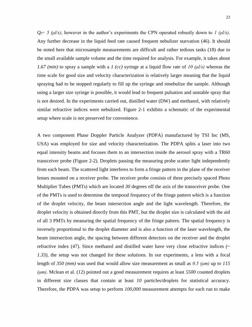
A two component Phase Doppler Particle Analyzer (PDPA) manufactured by TSI Inc (MS,

USA) was employed for size and velocity characterization. The PDPA splits a laser into two

equal intensity beams and focuses them to an intersection inside the aerosol spray with a TR60

transceiver probe (Figure 2-2). Droplets passing the measuring probe scatter light independently

from each beam. The scattered light interferes to form a fringe pattern in the plane of the receiver

lenses mounted on a receiver probe. The receiver probe consists of three precisely spaced Photo

Multiplier Tubes (PMTs) which are located 30 degrees off the axis of the transceiver probe. One

of the PMTs is used to determine the temporal frequency of the fringe pattern which is a function

of the droplet velocity, the beam intersection angle and the light wavelength. Therefore, the

droplet velocity is obtained directly from this PMT, but the droplet size is calculated with the aid

of all 3 PMTs by measuring the spatial frequency of the fringe pattern. The spatial frequency is

inversely proportional to the droplet diameter and is also a function of the laser wavelength, the

beam intersection angle, the spacing between different detectors on the receiver and the droplet

refractive index (47). Since methanol and distilled water have very close refractive indices (~

1.33), the setup was not changed for these solutions. In our experiments, a lens with a focal

length of 350 (mm) was used that would allow size measurement as small as 0.5 (μm) up to 115

(μm). Mclean et al. (12) pointed out a good measurement requires at least 5500 counted droplets

in different size classes that contain at least 10 particles/droplets for statistical accuracy.

Therefore, the PDPA was setup to perform 100,000 measurement attempts for each run to make

24

sure these requirements are met. Each single run (size and velocity measurement) was repeated

at least 3 times. The standard deviation between the runs was generally small (less than 1-2%).

Thus the statistical errors are negligible and will not be reported hereafter. The results of the 3

different runs were then combined to assure the experiments were not run-dependent. It is worth

mentioning some difficulties associated with droplet size and velocity measurements of

pneumatic nebulizers working under realistic conditions with PDPA instruments. First, PDPA

requires a high level expertise to acquire good results since it’s rather a complicated optical

device (12). In addition, there must be a high probability of having only one particle in the

sample volume at one time but the pneumatic nebulizers have generally high particle number

densities of the order of 106 particles per cm

-3 (48). Furthermore PDPA measurement is only

useful for spherical droplets. Irregular or deformed droplets yield irregular light scattering

patterns and are not reliably measured, especially close to the nebulizer tip (12). Thus all the

measurements were taken 10 (mm) downstream of the nebulizer tip along the axis to avoid high

rejection rate in the dense spray region and the interference of the laser beam with the

experiment setup. However, numerous measurements were also carried out at different axial and

radial locations to study the local spray characteristics. The PDPA device had to be calibrated to

assure good and reliable spray measurements. The calibration procedure is not included in this

chapter but can be found in Appendix B. Table 2-1 presents a summary of the experiment setup

and the devices exploited in the experiments.

Nukiyama–Tanasawa Correlation 2.2

Atomization is the process of converting a bulk liquid into a multiplicity of small drops in order

to produce a high ratio of surface area to mass in the liquid phase, favoring heat and mass

transfer processes such as evaporation. Conventionally, atomization is accomplished by applying

a high relative velocity between the liquid and surrounding gas phase so that the disruptive

aerodynamic forces overcome the consolidating surface tension forces. This goal is achieved

either by injecting a high velocity liquid into quiescent gas as in the case of plain orifice and

pressure swirl atomizers or in contrary by exploiting a high velocity gas stream to disintegrate a

slow moving liquid flow as in twin-fluid, airblast and air-assist atomizers.

25

Operating conditions of nebulizers

TR30-C3 CPN

Gas, Gas flow rate Argon, 0.2-0.8 (l/min)

Liquid, Liquid flow rate Distilled Water/Methanol, 1-10 (μl/s)

Applied gas pressure 35-210 (KPag)

Geometrical parameters

Gas annular area (0.03 mm2), Capillary ID (260

μm), Capillary tip recess (500 μm), Tabulation

OD (6mm), Fluid inputs (4mm)

FFN

Gas, Gas flow rate Argon, 0.15-0.21 (l/min)

Liquid, Liquid flow rate Distilled Water/Methanol, 0.1-1 (μl/s)

Applied gas pressure 35-70 (KPag)

Geometrical parameters Capillary ID (175 μm), Capillary OD (1/32”),

Tube OD (3.2 mm), Tube thickness (250 μm),

Capillary tip recess (300 μm/ variable), Orifice

(150 μm)

Mass flow controller and readout MKS-Type246C (MKS Instruments, MA,

USA)

Syringe 5cc-plastic (Becton Dickinson, ON, Canada) -

1cc-glass (Hamilton Company, NV, USA)

Syringe pump Model-22 (Harvard apparatus, MS, USA)

Rotameter Model-PMR1-010537 (Cole-Parmer Canada

Inc, QC, Canada)

PDPA parameters

Off axis angle 30○

Focal length 350 (mm)

Droplet size measurement range 0.5-115 (μm)

Number of measurement attempts 100,000

Table 2-1: Operating conditions for nebulizers and the measurement devices exploited in

experiments

Lefebvre states that airblast and air-assist atomizers have advantages over pressure atomizers

because they require lower liquid pressures and generally produce a finer spray (49). The

physical processes involved in atomization are still not well understood. Hence the majority of

studies in this field suffers from lack of knowledge about the microscopic foundations of aerosol

generation and is empirical in nature. Nevertheless these empirical studies have yielded a

considerable body of information on the atomization phenomenon such as the effect of liquid and

26

Fig

ure

2-1

: E

xper

imen

t se

tup,

das

hed

lin

e re

pre

sents

mak

eup g

as l

ine

and i

s only

use

d f

or

FF

N.

27

Fig

ure

2-2

: S

chem

atic

of

PD

PA

and f

iber

opti

cs.

28

gas properties, nozzle geometry, liquid and gas flow ratios, etc. (50).

The first major study on airblast atomization was conducted by Nukiyama and Tansawa in 1939

for characterization of a plain-jet airblast atomizer (51) by collecting droplets on oil-coated glass

slides. The authors investigated different parameters influencing the atomization process and

proposed a correlation for the Sauter mean diameter (D32), a characterstic moment which

represents the mean volume to mean surface area of the spray. For instance, they figured out by

lowering surface tension and liquid viscosity and increasing the liquid density a finer aerosol is

generated. They also showed that the spray Sauter mean diameter can be controlled through the

following dimensionless numbers:

(

√

√

√ ) (2-1)

Here UR, ζ, ρl, do, ηl, Ql and Qg are the relative velocity between the gas and liquid at the

nebulizer exit, surface tension, liquid density, orifice diameter, liquid viscosity, liquid and gas

flow rates respectively. By rearranging Equation (2-1):

(

√

√ √

√ ) (

√ √

) (2-2)

where Wed0 and Ohdo are Weber and Ohnesorge numbers based on the orifice diameter, the two

diemsnionless numbers which usually appear in droplet size characterization studies.

Nevertheless, in the Nukiyama and Tanasawa experiments the gas velocity was kept well below

sonic conditions (20). Thus the gas density is essentially constant. Besides the authors found that

varying the orifice diameter does not significantly affect the Sauter mean diameter. Thus, for

constant gas density and neglecting orifice diameter, Nukiyama and Tanasawa derived the

following correlation from Equation (2-1).

)

(

)

(

√ )

(

)

(2-3)

29

Please note in the absence of nozzle geometrical parameters, i.e. orifice diameter here, Equation

(2-3) is essentially non-dimensionalized meaning that correct units must be used for each

parameter. Here D32, ζ,UR,ρl,ηl, Ql and Qg must be given in (μm), (dynes/cm), (m/s), (g/cm3),

(poise) and (l/min) respectively. In addition Equation (1-3) is defined for a specific ranges of

flow parameters, 0.8< ρl<1.2 (g/cm3), 30<ζ<73 (dynes/cm) and 0.01<ηl<0.8 (poise). The

relative velocity (UR=ug-ul) must be calculated from known liquid and gas velocities. The liquid

velocity is simply calculated by dividing the recorded liquid flow rate by the capillary cross

sectional area but the same procedure may not be used for the gas velocity calculation due to

compressibility effects. Therefore, the gas velocity is estimated from isentropic theory from the

gas back pressure and the atmospheric pressure (52):

(

)

(2-4)

(

)

(2-5)

(

)

(2-6)

√ (2-7)

here Pg,Tg and ρg are the gas exit absolute pressure, absolute temperature and gas density. Exit

pressure has a value of P= 102.9 (KPag) when the flow is not chocked, i.e. when the back gauge

pressure is below 108.3 (KPag). P0, T0 and ρ0 are back or absolute stagnation pressure,

temperature and density where T0 is assumed to be 293 (K) and P0 is adjusted via the pressure

regulator. M is the Mach number whereas u* represents the sonic velocity. k and R are the ratio

of the specific heats of the gas at constant pressure and volume (k=cp/cv) and gas constant

respectively. For Argon k and R are 1.667 and 208.11 (J/kg.K) respectively. It should be noted

that the assumption of one dimensional isentropic flow in an ICP-MS nebulizer may not be true

as the flow irreversibilities and the nebulizer geometry will cause a deviation from the isentropic

condition. However as stated in reference (20), the isentropic flow approximation is valid for

30

nozzles as small as 200 (μm). Hence the isentropic theory provides a good engineering

approximation of the gas exit velocity required in Equation (3-2). Based on the isentropic theory,

the sonic condition is met when the back pressure is 108.3 (KPag). For the CPN nebulizers

however, the sonic condition may be delayed to 175-315 (KPag). This uncertainty has little

effect on the D32 calculation (Equation 1-2) since the second term of Equation (3-2) is dominant.

Figure 2-3a-c compares the Sauter mean diameter variation with gas flow rate from the NT

model and experiment for distilled water (DW) and methanol at different liquid flow rates. As

can be seen, the lower surface tension of methanol has resulted in a decrease of D32 as expected.

The difference between model prediction and experiment is more noticeable at higher liquid

uptake rates. The NT model shows a dropping trend in the Sauter mean diameter with the

increase of gas flow rate although the predicted size is largely overestimated. In our experiments

for instance, the maximum overestimation is up to 4 fold the measured size and this trend is more

obvious for higher liquid flow rates. Similarly, in flame atomic spectrometry although the range

of gas flow is larger than ICP-MS, there are reports of up to 30 folds overestimation for the

organic solvents (53). Furthermore, Figure 2-3a-c and Figure 2-4a-b demonstrate that for each

liquid flow rate, the error in the prediction grows larger with decreasing gas flow rate, i.e. with

smaller liquid to gas flow ratio.

The gas velocity at the nebulizer exit is orders of magnitude larger than the typical liquid

velocities. Thus it is reasonable to assume that the relative velocity is little influenced by the

liquid. Besides, if the isentropic theory (Equations 2-4 to 2-7) is employed to predict gas exit

velocity, the first term of the NT model reaches a minimum plateau when the sonic condition is

met at 108.3 (KPag). Sharp (20) has argued that the adiabatic condition may not be met, at least

for long nebulizers, and the internal heat generation due to friction will cause a deviation from

the isentropic theory that leads to slightly higher exit temperature and gas velocity. Nevertheless,

the deviation may not make a pronounced difference in the exit condition and the contribution of

the first term in the NT model is predetermined.

31

(a)

(b)

0

5

10

15

20

25

30

35

0 200 400 600 800 1000

D32 (

µm

)

Qg (ml/min)

Ql=1 (µl/s)

Experiment, DW

NT, DW

Experiment, Methanol

NT, Methanol

0

10

20

30

40

50

60

70

0 200 400 600 800 1000

D32 (

µm

)

Qg (ml/min)

Ql=5 (µl/s)

Experiment, DW

NT, DW

Experiment, Methanol

NT, Methanol

32

(c)

Figure 2-3: Sauter mean diameter versus gas flow rate for distilled water and methanol from

experiment and the original NT model at (a) Ql=1 (µl/s), (b) Ql=5 (µl/s) and (c) Ql=10 (µl/s).

Hence the overestimation of size is mainly due to the weight of the second term of the NT model

as reported by Sharp (20), Robles et al. (53) and Canals et al. (54). For instance, Figure 2-5

shows that the contribution of first term increases while at the same time that of the second term

decreases by increasing the gas flow rate. The dominance of the second term is more pronounced

at high liquid flow rates, that is 76-50 percent of the total D32 value at Ql=10 (µl/s), 53-26

percent at Ql=5 (µl/s) and 9-3 percent at Ql=1 (µl/s). It should be noted that as far as the validity

of the experiments is concerned, our experimental results at Ql=10 (µl/s) and variable gas flow

rates with TR30-C3 nebulizer is very similar to those of reference (54) with different Meinhard

concentric nebulizers.

At this stage it would be helpful to discuss the limitations of the Nukiyama – Tanasawa

correlation when applied to atomic and mass spectrometry. First as stated earlier, Nukiyama and

0

20

40

60

80

100

120

140

0 200 400 600 800 1000

D32 (

µm

)

Qg (ml/min)

Ql=10 (µl/s)

Experiment, DW

NT, DW

Experiment, Methanol

NT, Methanol

33

(a)

(b)

Figure 2-4: Error between experiment and the original NT model grows larger by

increasing the liquid flow rate for (a) distilled water and (b) methanol.

0

50

100

150

200

250

300

0 200 400 600 800 1000

Qg (ml/min)

100×(D32experiment-D32

NT )/ D32

experiment

Ql= 1 µl/s

Ql= 5 µl/s

Ql= 10 µl/s

0

100

200

300

400

500

600

0 100 200 300 400 500 600 700

Qg (ml/min)

100×(D32experiment-D32

NT )/ D32

experiment

Ql= 5 µl/s

Ql= 10 ul/s

34

Tanasawa observed no strong mean diameter dependence on the nozzle geometry (51), but at no

time did they test their correlation for a nozzle with dimensions similar to modern CPNs.

For example, in the Nukiyama and Tansawa experiments, the gas to liquid jet diameter ratio was

between 5 and 17 (liquid jet diameter 0.2-1.0 mm and gas jet diameter 1-5 mm) which is not

comparable to a 250 (µm) liquid capillary and gas annulus thickness of 20-30 (µm). Second, their

nozzle was operated well below the sonic point and as a result, compressibility effects did not

come into the picture. But ICP-MS nebulizers are usually employed at the sonic point or may

even surpass it. Third, back in 1939, Nukiyama and Tanasawa’s measurement technique was

rather primitive. The authors had to collect droplets on oil-coated slides and measure the drop

sizes under a microscope. Therefore it wouldn’t be a surprise to believe that their correlation

could be to some extent biased in favor of larger mean droplet moments. Gretzinger and Marshal

(55) claim that application of Equation (3-2) for the range of 5-30 (µm) is doubtful although the

model is proposed for the range of 15-90 (µm) mean sizes (56).

Figure 2-5: Contribution of first and second term in Nukiyama – Tanasawa equation. Δ: Ql=1

(µl/s), ○: Ql=5 (µl/s) and ◊: Ql=10 (µl/s). Dashed and solid lines represent first and second

term of Nukiyama - Tanasawa equation respectively.

0

10

20

30

40

50

60

70

80

90

100

0 200 400 600 800 1000

Per

cen

t

Qg (ml/min)

Weight of first and second terms in Nukiyama-

Tanasawa equation

Term2/D32NT

Term2/D32NT

Term2/D32NT

Term1/D32NT

Term1/D32NT

Term1/D32NT

35

It should be noted however, that the CPNs normally generate aerosol with Sauter mean diameters

in the range of 10-50 (µm) based on the liquid and gas flow parameters as shown in Figure 2-6.

The Figure 2-6 also demonstrates a peak value of 9.4 (µm) that is of the correct order as

predicted from the optimized wavelength calculation performed in the previous chapter (Refer to

pages 9-10).

Finally and most importantly, liquid and gas flow ratios in the Nukiyama and Tanasawa

experiments are very different from ICP-MS. The typical CPN employs a gas flow rate of up to

1000 (ml/min) with a liquid sample uptake rate of 50 (µl/s). For this range of flow parameters,

the flow ratio is not comparable to the Nukiyama-Tanasawa study (51). The liquid to gas flow

ratio (Ql/Qg) varies between 0.0001 - 0.001 in the 4th

report of the Nukiyama-Tanasawa study

where the NT model was proposed for the first time. This would imply that the ratio (1000Ql/Qg)

will be well below unity after exponentiation in Equation (3-2) and guarantee no severe

overestimation. For instance, at Ql=1 (µl/s) of Figure 2-3a, the gas to liquid flow ratio is between

0.08 - 0.23; the second term constitutes 10 percent of the overall predicted size at most (Figure

2-5) and the overestimation is not severe. By increasing the liquid flow rate to 5 and 10 (µl/s),

i.e. increasing the liquid to gas flow ratio, the predicted size becomes drastically over estimated

and the weight of the second term becomes markedly pronounced (Figure 2-3b-c and Figure

2-5). Furthermore, for any desired liquid flow rate, decreasing the gas flow rate would also lead

to size over prediction. For instance the largest error in Figures (Figure 2-3a-c) is seen at

Qg=260-280 (ml/min) which again signifies the effect of the liquid to gas flow ratio.

Consequently, application of Equation (3-2) to mass and atomic spectrometry in its original form

is under question (54) with only a few exceptions such as (57), (58) and (59). However the

results of these exceptions cannot be generalized because either the experiments were carried out

for a single case or specific range of liquid and gas flow rates that fit into the Nukiyama –

Tanasawa correlation. Another common misuse of the NT model in the atomic and mass

spectrometry is the model implementation for estimating tertiary aerosol, i.e. the aerosol leaving

the spray chamber (57), however the NT model is proposed for primary aerosol restrictively and

36

its employment for modified aerosol is not logical even though it may produce seemingly

acceptable results.

Despite all the criticism of the NT model and its rather restricted boundary conditions (60), the

correlation is still the most widely quoted work in pneumatic atomization (61) and sample

introduction in ICP-MS literature and holds general validity at least in describing the trends of

the physical processes involved in atomization. In the absence of superior models it is still used

for modeling aerosol in MS (57), (62), (63), etc. In addition Montaser and Goligthly (10) believe

that Equation (2-3) shows good agreement between different methods of measurement and

theoretical approaches, thus its merit cannot be easily nullified and a lot of research must be done

before the Nukiyama – Tansawa correlation is regarded as useless in the field of mass and atomic

spectroscopy.

For instance, Kahen et al. (9) modified the NT model, for a DIHEN working at Ql=10-500

(µl/min) and Qg=0.2-1.0 (l/min) with different organic solutions and achieved satisfactory

agreement with experiment. To the author’s knowledge this is the only attempt reported in the

MS literature to modify the NT model for successful application in ICP-MS. Kahen et al.’s

model (MNT) assumes new coefficients for surface tension and viscous terms and also considers

an exponential decay type function for the liquid to gas flow ratio:

) (

)

(

√ )

(

) (2-8)

The coefficients P1 and P2 were obtained through curve fitting and are 86.4 and 105.4

respectively.

To verify the applicability of the MNT model, Equation (2-8) was tested for TR30-C3 CPN.

Figure 2-7 demonstrates a severe underestimation of D32 with the MNT model and the

corresponding curve seems almost flat. This is in part because DIHEN generally produces finer

spray in comparison to type C CPN under similar flow conditions, and at some gas and liquid

flow rates which are specifically attributed to DIHEN, TR30-C3 cannot generate aerosol at all. In

addition, Equation (2-8) has been proposed for a very narrow range of D32, varying from 4.6 to

7.2 (µm). Therefore, we can say that the MNT model is restrictively applicable to the

37

D (um)

dN

/dD

20 40 60 80

0.5

1

1.5

characterized DIHEN and perhaps with some leniency to some other micro nebulizers with

similar dimensions and comparable operating conditions.

Hence, we were motivated to modify the original NT model (Equation 2-3) for TR30-C3 CPN

under conditions mentioned in Table 2-1. We proposed to keep the structure of the original

model and apply the modifications through two coefficients as Kahen et al. (9) and also through

the exponent of the troublesome liquid to gas flow ratio. The new model is called fitted NT

(FNT) to avoid confusion with NT and Kahen et al.’s MNT models.

)

(

)

(

√ )

(

)

(2-9)

The coefficients A, B and C are found by minimizing the quadratic difference between

experimental and calculated values of Sauter diameter from Equation (2-9). The generalized

reduced gradient method embedded in Microsoft Excel Solver, a developed version of the so-

called GRG2 code (64), was employed for this purpose.

Figure 2-6: Typical size distribution with TR30-C3 CPN at Ql=5 (µl/s) and Qg= 500 (sccm),

liquid: distilled water. D32=20.8 (µm), Dpeak=9.4 (µm).

38

Coefficients A, B and exponent C for the fitted model are given in Table 2-2 and can be

compared with those of the NT (Equation 2-3) and the MNT (Equation 2-8) models. As can be

seen the first coefficient has been slightly reduced from NT to ONT models and the modification

is mainly done through the second coefficient and exponent implying that the weight of the first

term in Equation (2-9) has been considerably emphasized. In fact this term now constitutes over

80 percent of the predicted D32 value.

Figure 2-8a-c compares the FNT estimation with the experimental Sauter mean diameter in

which the model shows considerable improvement in comparison to the original NT model of

Figure 2-3a-c. Additionally, an asymptote is seen for the drop size as the nozzle meets the

theoretical sonic conditions, specifically for Ql=5 and 10 (µl/s), which was not seen before.

Figure 2-7 and Figure 2- also illustrate the improved agreement between model and experiment

where the previous 4 fold overestimation is dropped to a maximum of 1.2 times. The agreement

is particularly improved at higher liquid flow rates as the FNT points are populated along the 45

degree slope line in Figure 2- which implies a better prediction comparing to the original model.

It must be added that the proposed FNT model is not intended nor claims to be a universal

optimized substitute for NT but rather a correlation that characterizes a particular nozzle well

under the tested range of flow parameters. As mentioned before, geometrical parameters are

absent

Parameter NT model MNT model FNT model

A 585 86.4 569.9

B 597 105.4 148.7

C 1.5 Exponential decay fitted 0.37

Table 2-2: Coefficients and exponent of original NT, modified NT and the fitted NT models.

39

Figure 2-7: Sauter mean diameter versus gas flow rate from experiment, original NT model

and Kahen et al’s MNT model for distilled water at Ql=10 (µl/s).

in the NT correlation. Further research must be carried out with a wide range of the ICP-MS

nebulizers of different sizes and large range of fluid properties and gas to liquid flow ratios

before claiming to have a universal correlation for application to ICP-MS. However, it would be

interesting at this stage to test the validity of the FNT model (at least qualitatively) with other

studies. Noting that, although there are many published papers on nebulizer characterization for

ICP-MS in the literature, only a few of them have reported all the detailed parameters required

for a comparative study.

For this purpose, Canals et al.’s study was selected (65) in which authors proposed a 6-parameter

model for D32 prediction of 4 different Meinhard CPNs with different solutions under a range of

liquid and gas flow rates.

0

20

40

60

80

100

120

140

0 200 400 600 800 1000

D32 (

µm

)

Qg (ml/min)

Ql=10 (µl/s)

Experiment

NT

Kahen et al's MNT

40

(a)

(b)

0

5

10

15

20

25

30

35

0 200 400 600 800 1000

D32 (

µm

)

Qg (mlit/min)

Ql=1 (µl/s)

Experiment, DW

FNT, DW

Experiment, Methanol

FNT, Methanol

0

5

10

15

20

25

30

35

0 200 400 600 800 1000

D32 (

µm

)

Qg (ml/min)

Ql=5 (µl/s)

Experiment, DW

FNT, DW

Experiment, Methanol

FNT, Methanol

41

(c)

Figure 2-8: Sauter mean diameter versus gas flow rate for distilled water and methanol from

experiment and the FNT model at (a) Ql=1 (µl/s), (b) Ql=5 (µl/s) and (c) Ql=10 (µl/s).

( ) ( ) [ ( ) ] (2-10)

where coefficients Pij’s depend on nozzle geometry and flow conditions and are tabulated in

(65). Although the study is quite extensive from the point of view of the experiments carried out

and the model has yielded satisfactory results, the author believes it suffers from some issues.

First, it is not a simple and easy correlation to use and the coefficient for each specific

configuration of nebulizer and solution must be taken from a table. Second, the given form of the

correlation (Equation 2-10) certainly does not show the direct dependence of D32 on important

parameters like nozzle geometry and also fluid properties such as surface tension, liquid and gas

densities and viscosities, although all these parameters are embedded in the Pij coefficients.

0

5

10

15

20

25

30

35

40

0 200 400 600 800 1000

D32 (

µm

)

Qg (ml/min)

Ql=10 (µl/s)

Experiment, DW

FNT, DW

Experiment, Methanol

FNT, Methanol

42

Figure 2-9: Ratio of calculated to measured Sauter mean diameter versus gas flow rate for

distilled water.

Table 2-3 compares Canals et al.’s model for two out of four tested nebulizers (specifications

given (65)) with D32 values from experiment, NT and the new FNT models. As can be seen from

the table, Sauter mean diameter is always larger for the M4 nebulizer which is also predicted by

NT and FNT models. The overestimation by the FNT model is certainly not as severe as the

original NT model. The highlighted areas in Table 2-3 are of particular interest since the flow

conditions are comparable to our experiments and as can be seen the agreement is quite

acceptable while the original NT shows a maximum of 21 fold overestimation! It should be

mentioned that the FNT model was characterized with a different CPN and liquid flow rates

generally smaller than this study and n-Butanol was never sprayed as a sample.

In a nutshell, the modification presented for NT in this work can very well fit into experimental

results in the range given by Table 2-3. Application of FNT to the different nebulizers and

solutions always yields better results than the original NT. The comparison of different

conditions in Table 2-3, also shows the most important parameters for NT type correlations are

0.5

0.6

0.7

0.8

0.9

1

1.1

1.2

0 200 400 600 800 1000

D32 c

alc

ula

ted

/D32 m

easu

red

Qg (ml/min)

Ql= 1 µl/s

Ql= 5 µl/s

Ql= 10 µl/s

43

Figure 2-10: Measured versus calculated Sauter mean diameter from the original NT and

fittedd NT (FNT) models.

the gas and liquid flow rates. The new FNT model can provide satisfactory predictions for other

nebulizers and solutions if their ranges of gas and liquid flow rates are comparable to this study.

Rizk–Lefebvre Correlation 2.3

In 1980, Lefebvre published an excellent comprehensive study on airblast prefilming type

nozzles used in gas turbine engines (49). Lefebvre investigated numerous correlations proposed

for different pneumatic atomizer nozzles and drew some general conclusions on the effects of air

and liquid properties on the Sauter mean droplet size. For low viscosity liquids such as water, he

found that the main factors governing D32 are surface tension, air and liquid densities and air

velocity, which clearly confirms the optimization we did in Equation (2-9). On the other hand for

0

20

40

60

80

100

120

140

0 10 20 30 40 50

Pre

dic

ted

D32

(µm

)

Measured D32 (µm)

FNT

NT

44

Nebulizer Ql

(ml/min)

Qg

(l/min) Solvent D32 (65). D32 exp D32 NT D32 FNT

M3 1.90 1.10 Water 10.74 11.1 79.71 25.59

M4 1.90 1.10 Water 11.09 12.6 74.32 20.34

M3 1.90 1.10 Methanol 5.41 5.7 73.59 14.83

M4 1.90 1.10 Methanol 5.61 6.0 73.97 15.3

M3 1.90 1.10 n-Butanol 7.41 7.3 147.12 23.08

M4 1.90 1.10 n-Butanol 7.52 7.9 147.52 23.47

M3 1.90 0.65 Water 17.43 17.0 157.92 31.0

M4 1.90 0.65 Water 18.02 20.5 158.95 32.0

M3 1.90 0.65 Methanol 9.55 10.9 159.28 21.0

M4 1.90 0.65 Methanol 10.04 11.3 159.93 21.6

M3 1.90 0.65 n-Butanol 12.21 12.8 321.08 29.08

M4 1.90 0.65 n-Butanol 12.7 13.2 321.75 29.73

M3 1.90 0.4 Water 37.15 * 320.66 49.05

M4 1.90 0.4 Water 38.09 * 322.34 50.69

M3 1.90 0.4 Methanol 22.53 21.0 325.91 29.88

M4 1.90 0.4 Methanol 23.69 20.9 326.96 30.90

M3 1.90 0.4 n-Butanol 29.50 23.4 660.94 35.7

M4 1.90 0.4 n-Butanol 30.35 22.1 662.03 36.76

M3 0.60 1.10 Water 8.42 9.5 20.12 14.33

M4 0.60 1.10 Water 8.70 12.1 20.73 14.92

M3 0.60 1.10 Methanol 4.05 4.8 17.47 11.26

M4 0.60 1.10 Methanol 4.27 5.3 17.85 11.63

M3 0.60 1.10 n-Butanol 6.02 5.5 30.65 17.68

M4 0.60 1.10 n-Butanol 6.13 6.6 31.05 18.07

M3 0.60 0.65 Water 15.83 15.6 39.93 21.92

M4 0.60 0.65 Water 16.35 16.0 40.97 22.93

M3 0.60 0.65 Methanol 7.74 8.8 35.72 16.25

M4 0.60 0.65 Methanol 8.12 9.9 36.37 16.89

M3 0.60 0.65 n-Butanol 9.61 9.9 64.67 23.78

M4 0.60 0.65 n-Butanol 9.97 11.0 65.34 24.43

M3 0.6 0.4 Water 32.53 27.1 76.26 33.33

M4 0.6 0.4 Water 33.51 * 77.94 34.97

M3 0.6 0.4 Methanol 19.13 15.6 69.95 23.40

M4 0.6 0.4 Methanol 20.04 16.3 71.01 24.43

M3 0.6 0.4 n-Butanol 23.59 17.8 129.79 31.84

M4 0.6 0.4 n-Butanol 24.27 19.2 130.88 32.90

Table 2-3: Comparison between the model (NT, FNT) and experimental values of D32 (µm).

*=inefficient nebulization

highly viscous liquids the air effects become more dominant and D32 is mainly determined from

liquid properties and especially viscosity. In addition Lefebvre (49) states that the viscosity has

45

an effect quite separate from air velocity as experimentally observed by Nukiyama – Tanasawa

(51) and many others. Therefore a correlation for mean drop size should include two terms, one

including air velocity and liquid density and a second term containing liquid viscosity

⟨ ⟩ ⟨ ⟩ (2-11)

For prefilming airblast atomizers, <D32>1 is governed by the Weber number:

⟨ ⟩

(

)

( ) (2-12)

here Lc is a characteristic dimension of the atomizer and represents its linear scale whereas Dp is

the prefilmer lip diameter, and several different sources cited in (49) suggest x~0.5 (Refer to

Equation 2-3 for instance).

From conservation of momentum in the liquid-gas region (66):

( ) (2-13)

or

(

)⁄

(2-14)

Substituting for UR in Equation (2-12) gives:

⟨ ⟩

(

)

(

) (2-15)

The viscous dominant term <D32>2 depends on Ohnesorge number, the ratio of the square root

of the Weber number to the liquid Reynolds number, as:

⟨ ⟩

(

)

( )

(2-16)

46

Substituting Ur from Equation (2-14) gives:

⟨ ⟩

(

)

(

) (2-17)

By combing Equation s (2-17) and (2-15), we’ll have:

(

)

(

) (

)

(

) (2-18)

The characteristic length Lc represents the dimension at the point or surface where the liquid first

meets the gas stream. For prefilming atomizers this would be the prefilmer lip diameter (Dp)

which is often replaced by the liquid capillary diameter for simplification (Lc=Dp=do). In

practice some secondary factors such as liquid Reynolds number and gas Mach number may

influence the atomization process in a manner which is not yet understood (67). To improve the

correlation and account for the secondary effects, the exponent of the first term was reduced

from 0.5 to 0.4 (67). Also if the gas velocity (ug) is replaced by the relative velocity (UR), the

influence of liquid to gas flow ratio must also be adjusted. In reference (67), a value of 0.4 was

suggested for the ratio. Therefore Equation (2-18) becomes:

(

)

(

)

(

)

(

) (2-19)

Equation (2-19) can be rearranged in the following form:

(

)

(

)

( )

(

) (2-20)

where the Weber number (Wedo) and Ohnesorge (Ohdo) numbers based on orifice diameter

appear consistent with Equation (2.2).

Coefficients A and B are atomizer dependent and must be found empirically. Rizk and Lefebvre

(67) found an excellent fit to experiment with values of A=0.48 and B=0.15 for their specific

nozzle.

47

The merit of Equation (2-19) is that unlike the Nukiyama-Tanasawa correlation (Equation 2-3),

it’s presented in nondiemnsionalized form meaning that any consistent units could be used for

calculation. The nozzle dimension is included in the correlation and the gas density is also

considered, although in the original paper (67), the gas velocity was in the range 10-120 (m/s) for

which the gas stream is very weakly compressible. The gas density in our experiment was

calculated from isentropic relation (Equation 2-6) and varies from 1.87 to 3.28 (Kg/m3).

The CPN can be regarded as a converging nozzle although its annular cross section is different

from the circular cross section of converging nozzles. Nevertheless, the parameter which is most

relevant to the flow state in a nozzle is the cross sectional area rather than its length or shape

(20). Therefore, like any other converging nozzle the maximum possible velocity for a CPN is

the sonic velocity. In this respect, the orifice based Weber number (Wedo) in Equation (2-20),

will have its maximum value when the sonic condition is met and remains constant. Similarly the

Nukiyama-Tanasawa correlation (Equation 3-2) suggests that the weight of the first term is

predetermined at the sonic condition and beyond. However, further increase of reservoir tank

pressure beyond 211.3 (Kpa) corresponding to sonic condition, would continuously increase gas

density and mass flow rate while the gas exit velocity remains sonic at the exit plane. As a result,

even at the constant sonic gas exit velocity, an improved atomization is expected. The effect of

liquid to gas flow ratio is only observed in the second term of the Nukiyama-Tanasawa

correlation (Equation 2-3). In contrast, in the Rizk-Lefebvre correlation (Equation 2-20) the ratio

appears in both terms and include the factors involved in atomization more realistically.

The Rizk-Lefebvre (RL) model has recently gained attention in spectrometry. Gras et al. (68)

applied the RL model to 3 nebulizers used for sample introduction in atomic spectrometry for the

first time and reported that while the model is capable of predicting the general trend of

phenomena; it lacks accuracy mainly due to differences in dimensions and operating conditions

between their nozzles and those used in the original study (67). The authors (68) then tried to

overcome the problem by tuning the general RL model (Equation 21-2) by tuning its exponents.

We call this model Gras’ modified RL or (MRL-G) for simplicity. The exponents for this model

are a=0.5, b=0.53 and d=0.49 respectively.

48

Kahen et al. (9) also modified the RL model for modeling the Sauter diameter from a DIHEN

used for micro sampling (MRL-K) but they applied the modifications through both coefficients

and exponents and attained satisfactory results but also state that their modification is very

nebulizer dependent and exhibits tremendous deviation if used on other nebulizers.

As in (9) and (68) and similar to the modification done for the NT model, we also fitted Equation

(2-21) for our specific range of flow parameters (69) but decided to keep the coefficients the

same as the original study (67) and (68). Coefficient B and exponent c are very similar in all the

studies. This is mainly because the term is more dependent on to the liquid viscosity effects and

for low viscosity, the weight of this term is more or less the same (Table 2-4).

(

)

(

)

(

)

(

) (2-21)

As can be seen from Table 2-4, the modification is primarily done through the first term to

account for different operating gas and liquid flow rates (FRL model). Since our ranges of

parameters are closer to Kahen et al.’s study (9), the obtained value for coefficient a is very

similar to their study.

Parameter RL model MRL-G model MRL-K model FRL model

A 0.48 0.48 0.54 0.48

a 0.4 0.5 0.31 0.3

b 0.4 0.53 0.5 0.34

B 0.15 0.15 0.16 0.15

c 0.5 0.49 0.48 0. 5

Table 2-4: Coefficients and exponents of different RL type correlations, RL=original Rizk-

Lefebvre model, MRL-G=Gras’ modified model, MRL-K= Kahen et al.’s modified model,

FRL= present fitted RL model

49

(a)

(b)

0

5

10

15

20

25

30

35

0 200 400 600 800 1000

D32 (

µm

)

Qg (mlit/min)

Ql=1 (µl/s)

RL

MRL-G

MRL-K

FRL

Experiment

0

5

10

15

20

25

30

35

40

0 200 400 600 800 1000

D32 (

µm

)

Qg (mlit/min)

Ql=5 (µl/s)

RL

MRL-G

MRL-K

FRL

Experiment

50

(c)

Figure 2-11: Sauter mean diameter versus gas flow rate for distilled from experiment and

different RL type models at (a) Ql=1 (µl/s), (b) Ql=5 (µl/s) and (c) Ql=10 (µl/s).

The original RL model and the modified models were applied to our flow conditions. The results

of these models together with our fitted model (FRL) are plotted alongside experiment. As can

be seen from Figure 2-11, the original RL model shows underestimation. This behavior was also

reported in (68) and (9). The FRL shows considerably better size prediction in comparison to the

RL and the MRL-G models and is closer to the MRL-K model. This is probably due to the fact

that in the MRL-G model, the range of flow parameters (particularly the liquid flow rate) was

larger than our experiment. In fact as stated in the Chapter 1, we have exploited the CPN not in

its nominal range but rather in its lower limit of aerosol generation in order to produce the finest

possible aerosol size and this range is closer to the micro sampling liquid flow rates of Kahen et

al. (9), thus the MRL-K model prediction is in better agreement with our optimized model.

Despite all the differences, it’s worth mentioning that the RL type correlation predicts size

diameters far better than Nukiyama-Tanasawa correlation (Equation 2-3), particularly at higher

liquid flow rates. Compare Figure 2-11b-c with Figure 2-8b-c for instance.

0

5

10

15

20

25

30

35

40

45

0 200 400 600 800 1000

D32 (

µm

)

Qg (mlit/min)

Ql=10 (µl/s)

RL

MRL-G

MRL-K

FRL

Experiment

51

Variation of Characteristic Mean Drop Sizes 2.4

Although D32 is the most widely used aerosol size characteristic moment used for heat and mass

transfer studies, it doesn’t sufficiently characterize an aerosol. McLean et al. (12) lists 14

different parameters for this purpose and states among them characteristic moment and the size

distribution are the most important ones in dictating the quality of aerosol.

Consider a nebulizer system that can produce perfectly monodisperse aerosol at certain

conditions of 10 (µm) for example, from the definition of Sauter mean diameter, D32 would also

be 10 (µm) and all these droplets are successfully consumed by plasma, that leads to a transport

efficiency of 100 percent. Now imagine another nebulizer that generates the same Sauter mean

diameter at the same flow condition but with quite polydisperse drop size, in this respect the

transport efficiency of the system can be significantly smaller than 100 percent, because the

mass of a single 20,30,50 and 100 (µm) droplet equals 8,27,125 and 1000 times of the 10 (µm)

droplets. Thus prediction of distribution functions is of significant importance particularly in MS

which is the subject of Chapter 5 of the present study.

Customary distribution functions are defined by two parameters: one characteristic moment and

the span or width of the distribution but as will be shown in Chapter 5, a distribution function

can similarly be specified by a number of characteristic moments and have a span comparable to

a distribution function defined by a moment and span directly through the method of Maximum

Entropy Principle (MEP).

Aside from Sauter mean diameter (D32), two other characteristic moments are required for the

analytical study of the aerosols in this study, which are mass mean diameter (D30) and another

nameless characteristic moment (D-10), that is aerosol surface area to its mass ratio, with the

following definition:

∑

(2-22)

∑

(2-23)

52

here ΔNi, Di and Ntot are number of droplets in class diameter Di and total number of droplets.

Therefore, not only each characteristic moment contains some information regarding the spray

individually but also their combination determines the shape of the size distribution function

such as location of the peak diameter, span and its skewness.

Figure 2-12a-b shows variation of (D30/D32) and (D30/D-10) ratios with the normalized gas flow

rate. The gas flow rate here is normalized by the predicted sonic gas flow rate at (Qg=494 ml/min

corresponding to 108.3 Kpag). The Figures show that while the first ratio is an ascending

function with gas flow rate, a reverse trend is observed for the second ratio. Besides, as can be

seen, the ratio is hugely affected by the variation in the normalized gas flow rate from 0.5 to 1.4

whilst the liquid flow rate shows considerably less influence. Thus it seems reasonable to present

the ratios as averaged values over entire liquid flows for each specific gas condition, i.e. only as

a function of normalized gas flow rate as follows:

(

)

(

)

(

)

(2-24)

(

)

(

)

(

)

(2-25)

Equations (2-24) and (2-25) will be used together with FNT (Equation 9-2) and FRL (Equation

2-21) correlations for predicting size distribution of CPN.

Figure 2-13a-b depicts the local variation of D30/D-10 and D30/D32 for CPN with downstream

axial location for the sample liquid flow rate of Ql= 5 (μl/s) respectively. As can be seen at any

axial location the D30/D-10 ratio decreases while D30/D32 ratio increases by growth of the gas flow

rate. Besides, for any gas flow rate, D30/D-10 the ratio drops with the axial location which is more

noticeable at lower gas flow ratios. The opposite trend is observed for D30/D32 ratio and again the

53

(a)

(b)

Figure 2-12: Variation of (a) D30/D32 and (b) D30/D-10 versus the normalized gas low rates at the

downstream axial location of z=10 (mm).

0.65

0.7

0.75

0.8

0.85

0 0.5 1 1.5 2

D30/D

32

Qg/Qgsonic

Ql=1 µl/s

Ql=5 µl/s

Ql=10 µl/s

Average

1.3

1.4

1.5

1.6

1.7

1.8

1.9

2

2.1

2.2

0.4 0.6 0.8 1 1.2 1.4

D30/D

-10

Qg/Qgsonic

Ql=1 µl/s

Ql=5 µl/s

Ql=10 µl/s

Average

54

(a)

(b)

Figure 2-13: Variation of characteristic moment ratio with axial location (a) D30/D-10 and (b)

D30/D32 at Ql=5 (μl/s).

1.1

1.2

1.3

1.4

1.5

1.6

1.7

1.8

1.9

2

2.1

0 10 20 30 40 50 60

D30/D

-10

z(mm)

Axial variation of D30/D-10

Qg=266(mli/min)

Qg=317 (ml/min)

Qg=390 (ml/min)

Qg=494 (ml/min)

Qg=590 (ml/min)

Qg=688 (ml/min)

Qg=786 (ml/min)

0.65

0.7

0.75

0.8

0.85

0.9

0.95

0 10 20 30 40 50 60

D30/D

32

z(mm)

Axial variation of D30/D32

Qg=266(mli/min)

Qg=317 (ml/min)

Qg=390 (ml/min)

Qg=494 (ml/min)

Qg=590 (ml/min)

Qg=688 (ml/min)

Qg=786 (ml/min)

55

gradient is a somewhat remarkable for Qg=266-390 (ml/min). Very similar trends are observed at

Ql=1 and 10 (μl/s) which are not shown here.

Nebulization Efficiency 2.5

The role of nebulizers in general is to convert liquid kinetic energy to surface energy, as a result

the surface area of the medium will be increased which in turn promotes the rate of heat and

mass transfer (49). The nebulizer efficiency is thus defined as the ratio of the spray surface

energy to the input kinetic energy of gas and liquid and also the thermal energy of the gas

stream.

The surface energy of droplets per unit time for an ensemble of droplets is:

∑ (2-26)

where n• has the unit (1/s). The consumed thermal energy (THE) and kinetic energy of the liquid

and gas (KE) is:

(2-27)

here ho is the total enthalpy of the gas whereas m•l and Ucap represent liquid flow rate and

velocity in the capillary. Sharp (20) states for short nozzles down to 200 (µm), the adiabatic

condition holds true and the total enthalpy remains constant (Δho=0). Thus by rearranging

Equation (2-27) we’ll have:

(2-28)

Besides, conservation of mass dictates:

∑

(2-29)

Therefore the nebulization efficiency will be:

56

( )

(2-30)

Since efficiency is below 100, we can define a minimum attainable D32 for an ideal nebulizer:

( )

(2-31)

(2-32)

The nebulization efficiency of the CPN under different flow conditions are plotted in Figure

2-14. The figure shows that first the efficiency drops by either decreasing the liquid flow rate or

increasing the gas flow, but more importantly it demonstrates that nebulization is generally a

very poor process as less than 1.2 percent of the input energy is converted to the surface energy.

In fact, nearly all the input energy is consumed for aerosol acceleration or wasted by the gas

expansion. The same trend is also reported for the efficiency of pressure atomizers (70) which

supports this trend. The minimum attainable D32 changes between 0.002-0.4 (µm) for all the

tested flow conditions, If the nebulization was only 10 percent efficient a D32 of 0.02 to 4 (µm)

would be obtained and most likely the entire aerosol would be consumable in the plasma without

perhaps any need for aerosol modification in a spray chamber.

In the derivation of the nebulizer efficiency, the conservation of mass was applied between the

liquid in the capillary and the droplets; however the measurements were taken 10 (mm)

downstream of the nebulizer tip along the centre line and not for the entire spray cross section.

This would introduce some error in efficiency calculation. Nevertheless in this location the spray

is not highly dispersed, i.e. the spray plume is very narrow and the spray cross section is small.

Further downstream where spray is considerably dispersed, D32 calculation along the centre line

may not represent the whole plane of droplets, besides the evaporation effects may also change

the spray size distribution, therefore Equation (30-2) must be used only for the primary aerosol.

57

Figure 2-14: Nebulization efficiency versus gas flow rates for distilled water measure at z=10

(mm).

It must be noted that the nebulization efficiency or transport efficiency, in ICP-MS literature (10)

is usually defined as the volume percent of the aerosol containing in droplets below 10 (µm)

(about 1-5 percent for a conventional CPN) but the definition given here is focused on the

conversion of input kinetic energy to surface energy of the aerosol or in other words the ratio of

minimum attainable to measured Sauter mean diameter.

Contribution 2.6

The CPN was characterized for a specific range of liquid and gas flow conditions. Although the

fundamentals of the nebulizer are very close to air-assist nebulizers, implementing the well

known correlations such as NT and RL lead to erroneous size predictions because the geometry,

dimensions and, more importantly, because the flow conditions are very different in ICP-MS

sample introduction. It was observed that the NT correlation severely overestimates the Sauter

0

0.2

0.4

0.6

0.8

1

1.2

0 200 400 600 800 1000

Eff

icie

ncy

(%

)

Qg (ml/min)

Ql=1 (ul/s)

Ql=5 (ul/s)

Ql=10 (ul/s)

58

mean diameter, while the RL model shows underestimation. The two models were then modified

considering the appropriate ranges of liquid and gas flow rate typical for ICP-MS applications

and a significantly better agreement with experiment was achieved comparing to the original NT

and RL models. Two correlations were proposed for the (D30/D32) and (D30/D-10) ratios which

contain information regarding the shape of distribution functions as will be discussed in the

Chapter 5. Furthermore, variation of these characteristic mean size ratios with axial location was

presented for different gas flow rates. A new nebulization efficiency was derived, introduced and

tested for the CPN under different flow conditions. This new definition of the nebulization

efficiency differs from conventional transport efficiency used in spectrometry. The present

definition focuses on the disintegration of the liquid bulk to the droplets or in the other words on

the conversion of kinetic energy to surface energy for atomization. It was found that from this

efficiency point of view, nebulization is a very poor process as only less than 2 percent of the

input kinetic energy is converted to the aerosol surface energy (for the given conditions). In

addition, a minimum attainable Sauter mean diameter for an ideal nebulizer from the efficiency

definition was obtained which could be useful for aerosol studies.

59

Chapter 3 Aerosol Size Characterization of Flow Focusing Nebulizer

Nozzle Design 3.1

The pneumatic Flow Focusing Nebulizer (FFN) is a relatively novel technology that was first

introduced by Ganan-Calvo (41) and (71). Due to the novelty of the technique, the number of

publications in this field is not comparable to other nebulizers, particularly those used for ICP-

MS sample introduction and despite the unique features of the nebulizer; it’s not commercially

available in the market.

The FFN has a simple design similar to plain-jet atomizers. As claimed in the literature (41), the

nebulizer can operate quite robustly with versatile flows to produce monodisperse spray. The

liquid sample experiences small shear forces associated with other micronebulizers with a solid

contact that may fracture or degrade some molecular species. Besides, as will be explained, in

this method the liquid does not touch the orifice and the necessary pressures are much smaller

than ones required to achieve comparable liquid jets using direct liquid injection leading to

increasingly lower risk of clogging and other operational costs. Furthermore, the nebulizer’s

geometrical parameters have very little influence on the nebulizer performance and the resultant

spray in contrast to concentric nebulizers described in Chapter 1. The simplicity of the

configuration also allows packing and multiplexing with only the restrictions imposed by

manufacturing constraints.

The aforementioned features, makes the nebulizer an excellent choice for ICP-MS applications,

at least theoretically. However there are currently only two papers published that have studied

the possible application of the FFN in spectrometry (42) and (43) where the results showed

superior aerosol generation in comparison to common micronebulizers.

Since the nebulizer was not commercially available, we have designed two prototype custom

designed FFNs in collaboration with Tanner’s group from the Department of Chemistry at the

University of Toronto (45). Figure 3-1 shows the schematic design of first prototype.

60

Figure 3-1: Schematic design of the first FFN.

35 mm

5 mm

61

As can be seen the nebulizer is equipped with two CCD cameras, one to view filament formation

in the pressurized tank section and the other one to observe downstream disintegration of the

filament into droplets whilst the area of observation inside the aperture was lighted by exploiting

an LED. A protective cap was placed under the planar orifice to secure it against displacement.

Inside the cap, there is a 5 (mm) diameter and 35 (mm) long aperture where the filament

disintegration takes place. In this design, a 100 (µm) plain orifice was laser drilled on a 25-50

(µm) stainless steel plate (Part FSS-3/8-DISK-100, Lennox Laser, Glen Arm MD) and was

placed 300 (µm) below the PEEK capillary tube of 360 (µm) OD and 125 (µm) ID (Upchurch

Scientific Inc., Oak Harbor, WA). The liquid was injected through the capillary with the aid of a

syringe and pump system. Inside the tank, pressure was built up by Argon flow feeding from the

nebulizing line. A separate makeup gas line was connected at 45 degree to the aperture and its

flow was directly controlled by a rotameter as shown in Figure 2-1. It’s worth noting that the

makeup gas has no role in aerosol generation and it only avoids aerosol deposition on the

aperture walls and assists in transportation of the aerosol toward plasma.

The prototype nebulizer shown in Figure 3-1 and Figure 3-2 was robust and worked stably down

to liquid flow rates of Ql=1 (µl/s) but, below this rate a stable filament was never formed.

Instead the nebulizer spit the liquid irregularly and frequent starvation was observed. To resolve

this problem and also recalling that this rate of flow is not suitable for microsampling, the

nebulizer was redesigned. The CCD cameras and LED components were removed from the

second design and the heavy steel structure was replaced by a long straight tube and steel

capillary (shown in Figure 3-3) whose critical dimensions are given in Table 2-1. With the

second design, we were able to lower the liquid flow rate to Ql=0. 1 (µl/s) and observe formation

of a stable filament under a microscope.

For characterization of the nebulizer and also the aerosol modeling through the Maximum

Entropy Principle (MEP), only the results of the second prototype were used. It’s worth noting

that the nebulizer makeup gas line was not used during characterization of the primary aerosol,

since its role is limited to the aerosol transportation and to some extent evaporation rather than

bulk liquid disintegration and spray formation.

62

Figure 3-2: The actual prototype of the first custom designed FFN.

63

Figure 3-3: Schematic design of the second FFN.

Theoretical Background 3.2

The gas flow used for nebulization builds up a pressure difference (ΔPg) across the nebulizer tip,

i.e. the orifice in Figure 3-3 or Figure 3-4. When this pressure difference is sufficiently large to

overcome the surface tension force of a liquid attached to the mouth of a capillary with diameter

(Dcap), it pulls the liquid toward the orifice (diameter do) and forms a cusp-like shape at a critical

distance from the orifice (H). If the liquid is constantly supplied through the capillary at the rate

(Ql), then a steady state liquid filament with diameter dj is emitted smoothly and extends few

millimeters depending on the flow conditions downstream of the orifice (Figure 3-4a-c).

Ganan-Calvo (41) has shown that the diameter of the liquid jet (dj) can be derived by solving the

one dimensional Navier-Stokes equation in the axial direction (along the nebulizer axis).

Consider the meniscus attached to the capillary in Figure 3-4. The diameter of the filament

changes with the axial

64

Figure 3-4: Photographs taken from inside and outside of FFN (41) showing (a)- Capillary and

liquid filament, (b)-The liquid jet exiting the orifice and (c)- Unstable wave growth on the

filament surface, breakup and droplet generation

location due to the suction effect of the gas expanding from the orifice and the tangential viscous

stresses (ηs) on the jet surface in the axial direction.

(

( )

) ( )

(3-1)

The shear stress term in Equation (3-1) may be neglected in comparison to the kinetic energy of

the fluid and the pressure difference providing that the orifice thickness (L) is smaller or

comparable to its diameter. The capillary equation in the radial direction requires that:

65

( ) (3-2)

In practice, the pressure difference ΔPg is larger than the surface tension forces. Thus, Equation

(3-2) will become:

(

( )

)

(3-3)

Integrating from the mouth of the capillary to the orifice exit, results:

(

) ( ) (3-4)

Since in FFN, the jet diameter is at least an order of magnitude smaller than the capillary and the

orifice diameter (dj<<Dcap & do,), the first term on the left hand side may be neglected and the

resulting jet diameter will be:

(

)

(3-5)

Equation (3-5) shows that first; the jet diameter is only controlled by the applied pressure

difference across the nebulizer tip and the liquid flow rate and second it is independent of liquid

properties like the liquid surface tension and viscosity. Besides, the jet diameter remains constant

up to the breakup point because the gas pressure after the exit remains constant (41).

Equation (3-5) may suggest any desired combination of ΔPg and Ql can be selected to generate a

liquid filament, however when the liquid kinetic energy is not large enough to overcome surface

tension forces no filament is formed. Therefore for any given pressure difference and surface

tension, a minimum sprayable liquid flow rate exists:

(

)

(3-6)

66

The velocity of the filament is calculated from the liquid flow rate and the jet diameter (3-5):

√

(3-7)

Equation (5-3) implies that for any liquid, the jet velocity from the orifice exit down to the

breakup point is controlled not by the liquid flow rate (Ql) but by the applied pressure difference.

In other words for a constant pressure difference, increasing the liquid flow rate will only grow

the jet diameter while keeping the jet velocity untouched.

The physics explained above remains valid as long as the nebulizer is working under the flow

focusing regime. Ganan-Calvo (72) has shown that for the ratios H/do>0.25, the liquid pattern is

flow focusing and the gas flow follows the liquid axially. If the ratio drops below 0.25, the flow

regime will change dramatically. The gas flow becomes radial, i.e. perpendicular to the

symmetry axis. As a result a stagnation point develops between the capillary and the orifice

which causes a portion of the gas to flow upward and mix with the liquid. In such a scenario, the

liquid jet vanishes and is replaced by a plume of unsteady chaotic liquid ligaments.

Once the gas exits the orifice, the cylindrical mixing layer between the gas stream and the

stagnant ambient gas becomes unstable from the classical Kelvin-Helmholtz instability. The

growth rate of the mixing layer depends on the Reynolds number of the flow and the formed ring

vortices of the order (ug/do). Taking a characteristic velocity of 200-300 (m/s) corresponding to

the range of gas flows in our experiments and an orifice diameter of 150 (µm), the resultant

frequency is of the order 1-2 (MHz), which is of the order of the liquid jet breakup frequency (fb~

(ζ/ρl×dj3)0.5

). Thus, the formation of the ring vortices excites the perturbation on the liquid jet

until it disintegrates into a plume of fine droplets (71). By tuning a resonance frequency through

the gas velocity or pressure difference driving the gas stream, one can apply the appropriate

wavelengths on the jet surface to generate drops of desirable sizes.

The breakup process of liquid jets is governed by the Weber number, that is the ratio of

aerodynamic forces to surface tension forces, and the Ohnesorge number, which shows the

relative importance of the stabilizing viscous forces.

67

(3-8)

( ) (3-9)

Please note in pneumatic nebulization, the gas velocity is orders of magnitude larger than the

liquid velocity, thus the relative velocity is substituted by the gas velocity in Equation (3-

8).Besides for the range of parameters in the experiments carried out, the expected jet diameter

changes between 3 and 12 (µm) and the Ohnesorge number is below unity. Thus, the viscosity

has little influence on either jet formation or disintegration (71), making the nebulizer an

excellent choice for introduction of organic based solutions containing cultured cells whose

fragile membranes are prone to rupture (41).

It’s also worth noting that formation of a small micron scale jet from Equation (3-5) does not

necessarily mean the resultant aerosols will have narrow size distribution. Ganan-Calvo (41) and

(71) states as long as the jet based Weber number (Equation 3-8) is kept below a critical value of

40, the aerosol shows monodispersity. At higher values of the Weber number, the time growth of

the non-symmetric perturbations is substantially shortened. Hence, both symmetric and non-

symmetric modes coexist which develops ligaments of different lengths that in turn leads to

higher degree of polydispersity. The jet based Weber number (Equation 3-8) in our experiment

varied in the range 5-30.

Figure 3-5 shows the orifice hole plate of the first prototype together with emitted micro jet for

distilled water at ΔPg=70 (Kpag) and Ql=1.66 (µl/s). The predicted jet diameter from Equation

(3-5) is 13.4 (µm) which is an order of magnitude smaller than orifice diameter of 150 (µm), as

can be noticed from the figure. Besides for the given conditions Equation (3-8) gives a jet based

Weber number of 26.1 that is below the critical value. Hence a relatively monodisperse aerosol

is expected. The number and volume distribution presented in Figure 3-6 shows high degree of

monodispersity for the mentioned flow conditions. For instance the standard deviation of the

number based distribution is 16 percent with mean, mass, Sauter and peak diameters of D10=19,

D30=19.5, D32=20, Dpeak=19.3 (µm) respectively. The close location of these characteristic

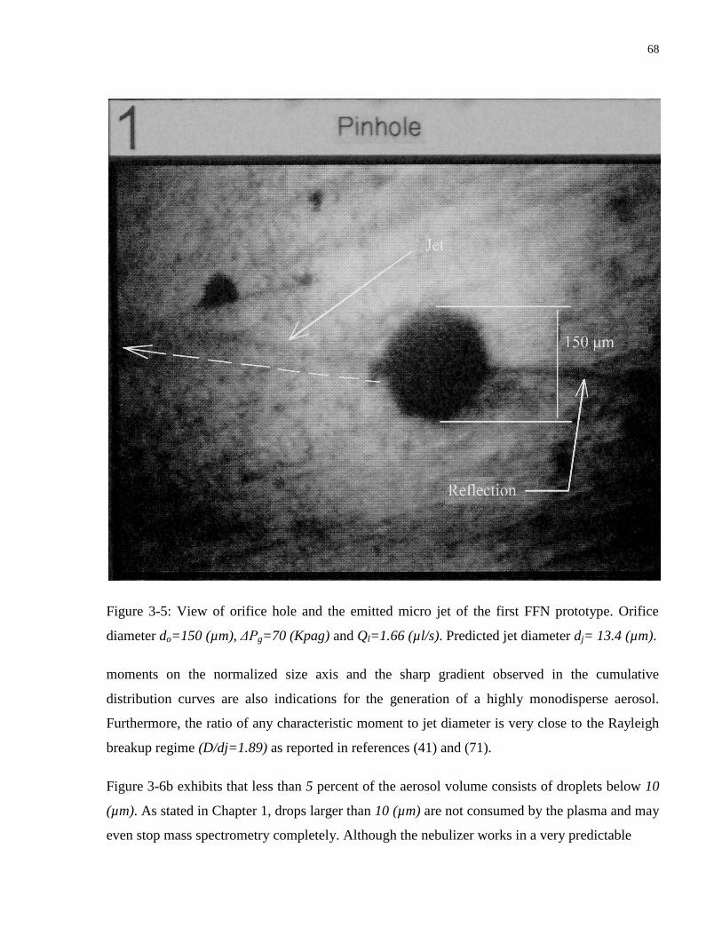
68

Figure 3-5: View of orifice hole and the emitted micro jet of the first FFN prototype. Orifice

diameter do=150 (µm), ΔPg=70 (Kpag) and Ql=1.66 (µl/s). Predicted jet diameter dj= 13.4 (µm).

moments on the normalized size axis and the sharp gradient observed in the cumulative

distribution curves are also indications for the generation of a highly monodisperse aerosol.

Furthermore, the ratio of any characteristic moment to jet diameter is very close to the Rayleigh

breakup regime (D/dj=1.89) as reported in references (41) and (71).

Figure 3-6b exhibits that less than 5 percent of the aerosol volume consists of droplets below 10

(µm). As stated in Chapter 1, drops larger than 10 (µm) are not consumed by the plasma and may

even stop mass spectrometry completely. Although the nebulizer works in a very predictable

69

(a)

(b)

Figure 3-6: Distribution curves for flow conditions given in Figure 3-5 (a) number and volume

distribution. (b) cumulative number and volume distribution.

D/D30

fn=

dN

/dD

,fv

=d

N/d

Vo

l

0.5 1 1.5 2 2.50

1

2

3

4

fn

fv

D (um)

cu

mu

lative

dis

trib

utio

n

0 10 20 30 400

20

40

60

80

100

Cumulative fn

Cumulative fv

70

manner and the results are in satisfactory agreement with literature, the quality of the aerosol at

the mentioned flow condition is not suitable for sample introduction. The atomization

performance may be improved by lowering the liquid flow rate but, unfortunately, the

employment of the first prototype below the liquid flow rate of Ql=1 (µl/s) led to very unstable

jet formation.

Another drawback of the first nebulizer is that the closest location for aerosols measurement was

5 (mm) below the cap and the aperture. By considering the 35 (mm) aperture length,

measurements were actually taken 40 (mm) downstream of the orifice exit. Obviously at this

location, a considerable portion of fine droplets may be lost due to deposition on the walls of the

aperture and some might have undergone secondary effects like collision and evaporation, thus

the distribution curves like those plotted in Figure 3-6a-b do not necessarily represent the

primary distribution of the aerosol. In addition, the gradual droplet deposition on the aperture

walls and their continuous downward motion would cause a liquid film formed at the mouth of

the aperture which would burst from time to time and interrupt the experiments.

In the second design of the FFN, the cap, aperture and CCD cameras were removed enabling us

to measure the primary aerosol as close as possible to the orifice exit and also lowering the liquid

flow rate below 1 (µl/s). From this point forward, all the characterization and modeling carried

out on the FFN are attributed to the second prototype, unless otherwise stated.

Droplet Size Modeling and Variation of Characteristic Mean 3.3Drop Sizes

The second FFN prototype was specifically designed as a direct injection nebulizer for

microsampling at low liquid flow rates (Ql= 0.1-1 µl/s). In all the experiments the nebulizing gas

flow rate was kept in a very narrow range of Qg=0.15-0.21 (l/min) in order to control the small

microjet and fine plume of aerosol. However, even for this narrow range, the Sauter mean

diameter changed between 6.6 (µm) to 21 (µm) corresponding to a jet diameter variation between

3.3 (µm) to 12.3 (µm), respectively. Due to very narrow range of flow parameters, unlike the

CPN, optimization of the NT and RL correlations does not seem reasonable but the two models

71

will be used for comparison. Groom et al. (73), proposed the following correlation for size

characterization of their flow focusing nebulizer:

[

(

)

]

(

) (3-10)

here Dcap is the liquid capillary diameter, and WeDcap and OhDcap are Weber and Ohnesorge

numbers based on the capillary diameter respectively.

The original RL model (Equation 21-2) shows that Weber number and liquid to gas mass flow

ratio acts in opposite direction and their exponents are of the same order of magnitude (Table

2-4). In addition, the exponent of the Ohnesorge number in Equation (21-2) is of the order of 1.

Groom et al. (73) also suggested j=1 for Equation (10-3). Nevertheless, the unknown coefficients

C1, C2 and the exponent m are nebulizer dependent and must be found from drop size

measurements. These parameters are given as C1=0.35, C2=0.25 and m=-0.75 for CPN and

C1=0.4, C2=0.4 and m=-0.6 for flow focusing nebulizer, respectively.

By taking the same approach and fitting Equation (3-10) for drop size measurements of the FFN,

C1=6.3, C2=0.31 and m=-0.84 resulted. The obtained exponent (m) is of the same order as

Groom et al.’s study (73) exhibiting similar drop size dependency to Weber number and liquid to

gas mass flow ratio. While C2 is very similar to the mentioned study, coefficient C1 is one order

larger than the reported numbers. However it should be noted that this coefficient is basically a

scaling factor and the reason for this difference is that first, the orifice and capillary diameter

were 2000 (µm) in the study in comparison to 150 and 175 (µm) here and second the liquid to

mass flow ratio was varied between 0.5-1.5 in (73) while it varies between 0.02 to 0.2 in the

present task.

Figure 3-7a-e demonstrates the predictions of the present model in comparison to the classical

NT and RL models. As for the CPN, the NT and RL show overestimation and underestimation

respectively although the dropping trend with increase of gas flow rate is clearly observed. The

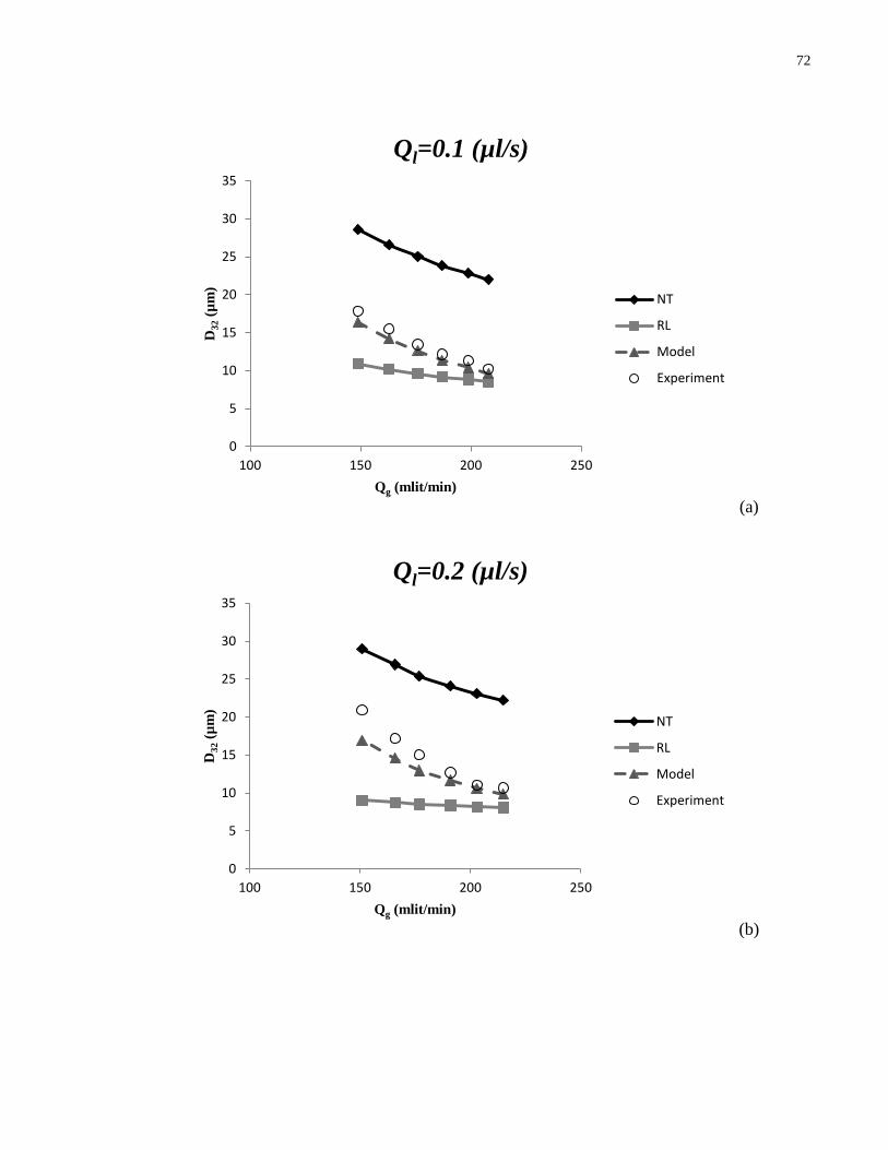
72

(a)

(b)

0

5

10

15

20

25

30

35

100 150 200 250

D32 (

µm

)

Qg (mlit/min)

Ql=0.1 (µl/s)

NT

RL

Model

Experiment

0

5

10

15

20

25

30

35

100 150 200 250

D32 (

µm

)

Qg (mlit/min)

Ql=0.2 (µl/s)

NT

RL

Model

Experiment

73

(c)

(d)

0

5

10

15

20

25

30

35

100 150 200 250

D32 (

µm

)

Qg (mlit/min)

Ql=0.4 (µl/s)

NT

RL

Model

Experiment

0

5

10

15

20

25

30

35

100 150 200 250

D32 (

µm

)

Qg (mlit/min)

Ql=0.6 (µl/s)

NT

RL

Model

Experiment

74

(e)

Figure 3-7: Comparison between drop size models and experiments at different liquid flow rates

for FFN at: (a) 0.1, (b) 0.2, (c) 0.4, (d) 0.6 and (e) 1.0 (µl/s).

present model (Equation 10-3), shows better agreement with the experiments that is noticed from

the figure.

As stated in previous chapter, the MEP modeling of the spray requires two size characteristic

moment ratios, hence as far as the modeling is concerned the variation of the dimensionless

ratios, rather than the characteristic moments, are of prime importance. Figure 3-8 depicts

changes in D30/D32 and D30/D-10 ratios with the normalized gas flow rate. Similar to the CPN

(Figure 2-12), an ascending and descending trend is observed for D30/D32 and D30/D-10

respectively. Although for Ql=0.1 (µl/s) similar trends are observed with the increase of

normalized gas flow rate, but the corresponding curve shows some degree of deviation from the

rest. Figure 3-8 suggests unlike CPN, the ratios are influenced by the liquid flows. In addition, a

close look at the distribution curves proves for any liquid flow rate at low gas flows, a weak

0

5

10

15

20

25

30

35

40

100 150 200 250

D32 (

µm

)

Qg (mlit/min)

Ql=1.0 (µl/s)

NT

RL

Model

Experiment

75

(a)

(b)

Figure 3-8: Variation of (a) D30/D32 and (b) D30/D-10 versus the normalized gas low rates at the

downstream axial location of z=10 (mm).

0.75

0.76

0.77

0.78

0.79

0.8

0.81

0.82

0.83

0.84

0.85

0.5 0.6 0.7 0.8

D30/D

32

Qg/Qgsonic

Ql=0.1 ul/s

Ql=0.2 ul/s

Ql=0.4 ul/s

Ql=0.6 ul/s

1.5

1.6

1.7

1.8

1.9

2

2.1

0.5 0.6 0.7 0.8

D30/D

-10

Qg/Qgsonic

Ql=0.1 ul/s

Ql=0.2 ul/s

Ql=0.4 ul/s

Ql=0.6 ul/s

76

bimodal behavior is observed which is resolved by increasing the gas flow rate that may account

for these irregularities of Figure 3-8. Please note that the axial and radial variation of the two

ratios is given in Appendix C.

Nebulizer Performance 3.4

The second FFN prototype was specially designed for microsampling applications, i.e. liquid

flow rates below Ql=1 (µl/s). For the range of flow parameters in our experiments, the predicted

jet diameter varies between 3 to 12 (µm) and a jet velocity of the order of 10 (m/s). The liquid

Reynolds number is therefore small (Reliq~30-150) and flow can be considered laminar. On the

other hand, the gas velocity calculated from the isentropic theory (Equations 2-4 to 2-7) is two

order of magnitudes larger than the liquid which leads to gas Reynolds number of (Reg=4000-

7000) based on the orifice diameter indicating strong turbulent behavior for the gas flow.

Although the breakup mechanism depending on relative velocity between the gas and liquid are

essentially the same for both pressure and airassist type atomizers, various flow phenomena such

as turbulence and cavitation are not observed in airassist atomization (50), consequently

atomization is solely depended on the momentum of the atomizing gas and air to liquid mass

flow ratio (Refer to Equations (3-10), (2-9) and (2-21) for instance).

Figure 3-9 shows the variation of characteristic size moments with jet based Weber number. In

this graph, the Rayleigh limit is plotted for comparison. Rayleigh (74) has shown for a laminar

breakup of a liquid jet in quiescent air, the resulted drop diameters are 1.89 times that of the jet

diameter. Weber (75) found that the effect of increased air friction on the jet (i.e. increasing

relative velocity) is to shorten the breakup length optimum wave-length that leads to smaller

drop sizes. For example D10, D30 and D32 are proportional to the Weber number to power -0.88, -

0.93 and -0.97, respectively.

It must be mentioned that the Rayleigh and Weber studies were carried out for laminar gas flows

and only presented the most probable drop sizes corresponding to the optimum wavelength,

different from the characteristic moments given here. Thus it seems reasonable to have

characteristic moments larger than the most probable droplet size particularly for higher order

77

Figure 3-9: Variation of characteristic moments of the primary size distribution with the jet based

Weber number measured at z=10 (mm).

moments like D30 and D32. The area marked in Figure 3-9 illustrates cases whose characteristic

moments are larger than the Rayleigh’s prediction. The jet breakup length in our experiments

was 1 to 3 (mm) while the measurements were taken 10 (mm) downstream of the nebulizer tip.

Therefore, coalescence might be responsible for the overgrowth of the characteristic moments at

this distance, particularly because it has occurred at low Weber numbers.

When the Weber number was increased over 10, the characteristic moments dropped below the

Rayleigh limit. This trend was continued down to moment to jet diameter ratio of 0.5-1

indicating an improved atomization at the Weber numbers around 20-25. Ganan-Calvo (41) and

(71) reported a Raleigh type breakup for Weber numbers below the critical value of 40. In other

words, the points are supposed to be populated around the Rayleigh limit in Figure 3-9, or

perhaps slightly below it (due to the increased drag effects). In addition, a fair comparison

between our results and those in (41) and (71) is not possible, since a similar graph was not

presented there. Besides, the aforementioned authors suffice to state below the critical Weber,

78

the distribution is very narrow and did not report monodispersity in full detail. For example, a

fine but polydisperse aerosol can be seen in Figure 8b-c of (71) and a very narrow one in Figure

8a of the same reference. The standard deviation of the primary size distribution for the FFN

versus the Weber number is plotted in Figure 3-10. As can be seen, in contrast to what is claimed

by Ganan Calvo (41) and (71), no clear relation can be found between the Weber number and the

span of the distribution. A closer look at our results show, the distribution becomes narrower by

increasing the Weber number for any desired liquid flow rate.

Based on these findings, we can say that the Weber number should not be used as a measure of

spray monodispersity/polydispersity, instead it’s the ratio of aerodynamic drag to capillary forces

by definition and merely reflects the degree of atomization.

Figure 3-11 to Figure 3-13 illustrate the number and volume-based size distribution together with

the corresponding cumulative distribution for 3 points of Figure 3-9. One, showing a large

characteristic moment to jet ratio, one close to the Rayleigh line and the last one in the region of

improved atomization, i.e. small moment to jet diameter ratio.

Figure 3-10: Standard deviation of the primary size distribution of the FFN versus the jet based

Weber number measured at z=10 (mm).

20

25

30

35

40

45

50

55

60

65

70

0 5 10 15 20 25

10

0*

Drm

s/D

10

Wedj

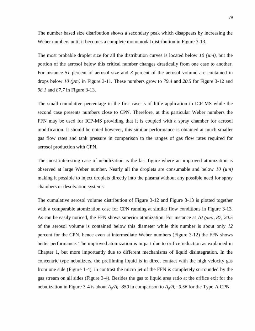
79

The number based size distribution shows a secondary peak which disappears by increasing the

Weber numbers until it becomes a complete monomodal distribution in Figure 3-13.

The most probable droplet size for all the distribution curves is located below 10 (µm), but the

portion of the aerosol below this critical number changes drastically from one case to another.

For instance 51 percent of aerosol size and 3 percent of the aerosol volume are contained in

drops below 10 (µm) in Figure 3-11. These numbers grow to 79.4 and 20.5 for Figure 3-12 and

98.1 and 87.7 in Figure 3-13.

The small cumulative percentage in the first case is of little application in ICP-MS while the

second case presents numbers close to CPN. Therefore, at this particular Weber numbers the

FFN may be used for ICP-MS providing that it is coupled with a spray chamber for aerosol

modification. It should be noted however, this similar performance is obtained at much smaller

gas flow rates and tank pressure in comparison to the ranges of gas flow rates required for

aerosol production with CPN.

The most interesting case of nebulization is the last figure where an improved atomization is

observed at large Weber number. Nearly all the droplets are consumable and below 10 (µm)

making it possible to inject droplets directly into the plasma without any possible need for spray

chambers or desolvation systems.

The cumulative aerosol volume distribution of Figure 3-12 and Figure 3-13 is plotted together

with a comparable atomization case for CPN running at similar flow conditions in Figure 3-13.

As can be easily noticed, the FFN shows superior atomization. For instance at 10 (μm), 87, 20.5

of the aerosol volume is contained below this diameter while this number is about only 12

percent for the CPN, hence even at intermediate Weber numbers (Figure 3-12) the FFN shows

better performance. The improved atomization is in part due to orifice reduction as explained in

Chapter 1, but more importantly due to different mechanisms of liquid disintegration. In the

concentric type nebulizers, the prefilming liquid is in direct contact with the high velocity gas

from one side (Figure 1-4), in contrast the micro jet of the FFN is completely surrounded by the

gas stream on all sides (Figure 3-4). Besides the gas to liquid area ratio at the orifice exit for the

nebulization in Figure 3-4 is about Ag/Al=350 in comparison to Ag/Al=0.56 for the Type-A CPN

80

(a)

(b)

Figure 3-11: (a) Number and volume-based size distribution and (b) Cumulative size and volume

distribution at Ql=0.2 (µl/s), Qg= 150 (milt/min), D10/dj=2.26 and Wedj=4.5, (point 1 in Figure

3-9).

D (um)

fn=

dP

/dD

,fv

=d

P/d

Vo

l

10 20 30 40

0.2

0.4

0.6

0.8

1

1.2

1.4

fn

fv

D (um)

cu

mu

lative

dis

trib

utio

n

0 10 20 30 400

20

40

60

80

100

Cumulative fn

Cumulative fv

81

(a)

(b)

Figure 3-12: (a) Number and volume-based size distribution and (b) Cumulative size and volume

distribution at Ql=0.6 (µl/s), Qg= 180 (milt/min), D10/dj=1.5 and Wedj=9.6 (point 2 in Figure

3-9).

D (um)

fn=

dP

/dD

,fv

=d

P/d

Vo

l

10 20 30 400

0.2

0.4

0.6

0.8

1

1.2

1.4

fn

fv

D (um)

cu

mu

lative

dis

trib

utio

n

0 10 20 30 400

20

40

60

80

100

Cumulative fn

Cumulative fv

82

(a)

(b)

Figure 3-13: (a) Number and volume-based size distribution and (b) Cumulative size and volume

distribution at Ql=1.0 (µl/s), Qg= 320 (ml/min), D10/dj=0.69 and Wedj=20.0 (point 3 in Figure

3-9).

D (um)

fn=

dP

/dD

,fv

=d

P/d

Vo

l

10 20 30 400

0.2

0.4

0.6

0.8

1

fn

fv

D (um)

cu

mu

lative

dis

trib

utio

n

0 10 20 30 400

20

40

60

80

100

Cumulative fn

Cumulative fv

83

Figure 3-14: Comparison between FFN and CPN running at comparable flow conditions Ql=1.0

(μl/s) and Qg~320-370 (ml/min).

of the Figure 1-2 which again may account for this improved atomization. It should also be

noted, even for the cases where atomization is not superior to CPN, the aerosol is formed from

disintegration of a micro jet which is two orders of magnitude smaller than the gas orifice and as

a result the solution leaves the orifice without touching it. This feature alone is a great advantage

for the FFN even if the nebulizer has to be coupled to a spray chamber. Please recall from

Chapter 1 that the micronebulization was mainly done through miniaturization of concentric

nebulizer at the cost of increasing the probability of frequent nebulizer clogging.

Contribution 3.5

In this chapter, the two custom designed FFN prototypes were first described and the

fundamentals behind the flow focusing nebulization were explained and finally the nebulizer was

D (um)

cu

mu

lative

vo

lum

ed

istr

ibu

tio

n

0 10 20 30 400

20

40

60

80

100

CPN @ Ql=1.0 (ul/s) and Qg=320 (ml/min)

FFN @ Ql=0.6 (ul/s) and Qg=180 (ml/min)

FFN @ Ql=0.1 (ul/s) and Qg=370 (ml/min)

84

characterized at different flow conditions and correlation (10-3) was fitted to the experimental

results.

It was shown that for small jet based Weber numbers, the coalescence effects are significant

which would result in mean to jet diameter ratios over the Rayleigh limit of 1.89. Increasing the

Weber number would decrease the ratio below the Rayleigh limit since the wavelength of the

fastest growing wave becomes smaller. Atomization was improved by further increasing the

Weber number beyond 20, where the mean to jet diameter ratio dropped to the values 0.5-1.0. It

was also shown that although Ganan-Calvo (41) and (71) state the Weber number is a measure of

spray polydispersity, a clear correlation between the two could not seen in this work.

The performance of the FFN was then studied and compared to the CPN. It was shown the FFN

generally produces a superior aerosol in comparison to the CPN. It was also shown that if the

flow conditions are tuned properly the FFN can provide aerosol with sufficiently large number of

consumable drops with diameters below 10 (µm), in other words the necessity of coupling the

nebulizer with spray chambers and desolvation systems may be removed and the nebulizer could

be used for direct injection of droplets to the plasma.

Another important feature of the nebulizer is that the improved atomization is not achieved by

miniaturizing the nebulizer dimensions as it is usually accomplished for conventional

micronebulizers and direct injection nebuilizers in the market. Because the mechanism of

atomization for this class of the nebulizers is different and since the sample does not touch the

gas orifice, the chance of the nebulizer clogging is theoretically reduced. This is feature could

have some interesting potentials for injecting slurry solutions. However separate quantitative

study on the nebulizer clogging for slurry solutions must be taken to prove the possible superior

performance of the nebulizer.

Although the FFN cannot be considered an ideal nebulizer at this stage and requires further

development, it has exhibited promising results. It must be noted that we have only presented

nebulizer characterization and aerosol modeling (Chapter 5). Since the technology is relatively

new and there are not many publications on the subject, further studies must be carried out to

investigate the analytical performance of the device integrated with ICP-MS instruments.

85

Chapter 4 Aerosol Velocity Characterization

General Considerations 4.1

The droplet size of the CPN and the FFN under different flow conditions were characterized in

Chapters 2 and 3 respectively. Introducing sample in ICP-MS however, requires controlling both

aerosol size and velocity since fast moving droplets won’t have enough time for adequate

vaporization and are source of noise and signal loss in ICP (38) and (76). In addition, aerosol

with wide ranges of velocities produce emission and mass spectrometric signals at different

locations in the plasma, leading to reduced sensitivity and signal fluctuations (65) and (76).

Therefore, not only size and velocity are of paramount importance, the primary aerosol (that is

the unmodified aerosol generated by the nebulizer) is a determining factor in transport efficiency,

nebulizer design and optimization of the operating conditions (9), (48) and (12). In this chapter,

the aerosol velocity of each nebulizer is characterized and the characteristic velocity moments

are presented. The results of size and velocity characterization will then be employed to model

the primary aerosol distribution through Maximum Entropy Principle (MEP) in Chapter 5.

As mentioned in Chapter 2, only the axial velocity component is studied for characterization

because drops passing along the nebulizer axis are more likely to reach the central channel of

ICP and contribute to MS signal (9). Kahen et al. (38), state that the velocity vectors in the

direction of the nebulizer axis are highly oriented at the central region and add that the residence

time of a droplet in ICP is proportional to the axial velocity whereas the other components has

little effect on this time scale. Other studies like (36) clearly shows for the primary aerosol, the

radial velocity component is smaller and negligible in comparison to the axial component

because small drops tend to lose their radial momentum rapidly upon leaving the origin of the

spray (77). A similar trend was also observed in our experiments except for locations farther

downstream where the spatial dispersion becomes important.

86

As the high velocity gas expands from the orifice in Figure 1-4, gas will be entrained from the

sides due to lower local pressure. The entrained gas in turn, drags small liquid drops from the

outer periphery of the spray inward and may even lead to eventual contraction of the spray (78)

that explains why large droplets are observed at the fringes of spray as reported in (9), (4), (18)

and many others and also our experiments. The magnitude of the contraction depends on such

parameters as the total flow rate, the size and initial velocity of the droplets and the gas density

(78). Schlichting (79) has given the analytical solutions for the flow fields of both laminar and

turbulent free jets issued from an infinitely small diameter and has shown that the governing

equations for both regimes are of similar form, with the assumptions that fluid is incompressible

and that the pressure in the jet is constant and equal to the surrounding pressure. Under these

conditions, the momentum of the jet would remain constant with the mass flow gradually

increasing as more fluid is entrained from the sides and the velocity gradually decreases.

Besides, it was also shown that the width of the jet is directly proportional to the axial location,

while the centerline velocity has inverse proportionality with the position. The entrained

volumetric flow rate in (79) is:

(4-1)

√ (4-2)

where ν is kinematic viscosity (ν=ηg/ρg), z is the downstream axial location from the nebulizer

orifice and θ is the kinetic momentum. The equations show that free jets entrain copious amounts

of gas and the volume doubling as the length doubles. Equation (1-4) surprisingly shows that for

a laminar jet, the entrained volume is independent of the initial momentum. Therefore a higher

velocity jet remains narrower over a larger length than one moving at a lower velocity. For

turbulent jets, which is our case, the entrained volume is proportional to the square root of the

initial momentum, however it is not possible to substitute values directly in Equation (2-4)

because for turbulent flows, knowledge of kinematic viscosity (εT) is a prerequisite ( √ ),

and this parameter unlike its laminar counterpart is not a fluid property but rather a characteristic

of the local flow.

87

Jets of finite width maintain a potential flow core until a point where the mixing zone width

equals that of the jet radius (80). Beyond this point, the whole jet is turbulent and the turbulence

is self-preserving because of the mixing process. For the self-preserving region of the jet, the

ratio of the volumetric flow rate Qz at position z, relative to the original volumetric flow rate

(Qo=ugπdo2/4) can be represented by the empirical correlation (81):

( )

(4-3)

here do is the orifice diameter, z’ is the distance from the apparent origin to the position where

the self-preserving part of the jet begins and A is a constant. The value of z’ depends on the

orifice type and values between z’=-0.5do to z’=-7do are reported in different sources. The

constant A also changes from study to study, but direct measurement entrainment by Rico and

Spalding (82) give a value close to 0.32. At a large distance from the orifice, Equation (4-3)

reduces to Qz/Qo=0.32z/do which is the form quoted in (80). Thus, for example a 100 (µm)

diameter jet in air, taking z’=-3do and A=0.32 at z=0.9 and 5.3 (mm), the ratio is Q/Qo=2 and 16

respectively. Besides, the reduced form of Equation (4-3) may be used to find the centerline axial

gas velocity, taking Qz=ug(z)πδ2/4 and recalling that jet width (δ) is proportional to axial location

(z), Equation (4-3) will then become:

( )

(4-4)

Equation (4-4) is only valid beyond the potential core of the turbulent jet that is about seven jet

diameter (80) when the turbulence becomes self-preserving, however in the presence of the

liquid phase; this length drops to about five times the jet diameter as reported in (31). In this

equation, the exit velocity at the orifice (ug), is calculated from the isentropic relations

(Equations 2-4 to 2-7) and remains unchanged within the potential core. Perry and Chilton (83)

have reported the constant K values of 5 and 6.2 for jet exit velocities of ug=2.4-4.9 (m/s) and

ug=10.0-51.8 (m/s) respectively. Gas jets of pneumatic nebulizers have higher velocities and

therefore a value of 6.4 was proposed for them by Tennekes and Lumley (84). Although this

value is given for air, it should be a reasonable approximation for argon because the magnitude

of the eddy viscosity reflects the state of the flow field rather than the molecular characteristics

88

of the gas (80). It should be noted that since Equation (4-4) is derived from Equation (4-3), it is

empirical in nature, thus other mathematical fits are also plausible. For instance, Pryds et al. (85)

have proposed an exponential decay for the gas velocity of an atomizer starting from the orifice

and neglected the potential core in their study. In the present study we’ll use Equation (4-4) to

predict the axial gas velocity because it is also a good measure for spray mean velocity.

The transverse (radial) distribution of the axial velocity is approximately Gaussian in shape and

may be estimated by (83):

( ( )

( )) (

)

(4-5)

Therefore the approximate axial gas velocity profile will be:

( ) ( (

)

) (4-6)

The effect of enclosing a free jet by either spray chamber as in the CPN or delivery tube for FFN

is very dramatic, since there is no longer an infinite reservoir of fluid available to feed the

entrainment process. The result is that the jet must entrain fluid from itself by forming

undesirable recirculation zones. The auxiliary (makeup) flow required for canceling the

recirculation and produce a uniform forward velocity is about 11.5 times the primary jet flow

(86) which is impractical for ICP-MS due to limitations on the injector flow.

Liu et al. (87) defines three distinct regions for the injection of a turbulent jet (Reynolds number

=3000 to 24000) from a nozzle into a straight pipe, a potential core and a self-preserving region

similar to free turbulent jets and a final region where the jet width equals the pipe diameter. This

region is significantly influenced by the wall effects and flow eventually becomes fully

developed. Hill (88), pointed out that under certain conditions, the mean velocity field in the self-

preserving region of the confined turbulent jet could be predicted from the free jet data, using no

other empirical information. Dealy (89) states the flow pattern of confined jets, in general should

depend on the ratio of the orifice diameter (do) to the pipe diameter (Dp) and the Reynolds

number (Re=ugdo/νg). However, for sufficiently large Reynolds number and with the assumption

89

of self preservation, the Reynolds number dependence can be neglected (87), whereas the

Reynolds number does not dictate the shape of the velocity profile in free turbulent jets (90).

As Liu et al. (87) explain the presence of the recirculation zone implies that the confined jet

feeds the required entrained fluid by itself and thus reduce its momentum which in turn leads to

smaller centerline velocity in comparison to the free turbulent case. The following correlation

was then proposed for do/Dp<<0.25 independent of the orifice shape:

( )

(

) (4-7)

where f is the velocity loss function and Dp is the pipe diameter. Since at the limiting case of

Dp→∞, Equation (7-4) must be reduce to Equation (4-4), a polynomial fit for f(do/Dp) was

assumed in (87):

( ) (

) (

)

(4-8)

Because the ratio do/Dp is generally small, the higher order terms in Equation (4-8) can be

neglected. The final form of correlation is given in (87):

( )

( ) (4-9)

Equation (4-9) can predict at what axial distance the direct injection nebulizer should be placed

so that the droplet velocities (assuming they are of the same order as gas velocity) fall in the

range 5-10 (m/s) to ensure total vaporization and consumption (76). Although the FFN and the

plasma is of very similar configuration, i.e. a nebulizer is placed either before the plasma torch or

inside a delivery tube, Equation (4-9) has been proposed for gas exit velocities of 5 to 66 (m/s)

which is smaller than the typical nebulizer gas exit velocity of ICP-MS (Recall a K value of 6.4

was proposed for turbulent free jet of Equation 4-4). Besides the makeup flow effects are also

not considered in Equation (4-9). Nevertheless, the study might be used as a guideline to

investigate the axial gas velocity of the confined FFN in the future. To the best of the author’s

90

knowledge, there is currently no study that directly relates the axial gas velocity of direct

injection nebulizers to the orifice to pipe diameter ratio and the makeup gas flow.

At this stage, it would be very useful to study the dynamics of a single particle travelling in a free

turbulent jet. Consider 1, 10, 20, 50 and 100 (µm) droplets axially injected at the exit of the

nebulizer with an orifice diameter of 260 (µm) through which argon flows at sonic velocity

ug=276.1 (m/s). Assuming that droplets are travelling along the centerline and do not disperse in

the plane normal to the nebulizer axis, the one-dimensional equation for the droplet motions is:

( ( ) )

(4-10)

here mp is droplet mass (mp=π/6×D3ρl), up is the droplet local velocity, CD is the drag coefficient

and Ac is the droplet cross sectional area (Ac=π/4×D2). Hence:

( ( ) )

(4-11)

The jet centerline velocity, ug(z), can be approximated by Equation (4-4) and isentropic theory

(Equations 2-4 to 2-7) that will remain constant for the first 5-7 orifice diameters until the

potential core is extinguished. Assuming that droplet can be modeled as non-deformable spheres,

calculation proceeds by considering a small axial increment and from the difference between the

gas and particle velocity a particle Reynolds number is calculated.

The drag coefficient is then evaluated by having the Reynolds number from (91):

(4-12)

Equation (4-12) is defined for Reynolds number in the range 0<Re<2×105. Although the

equation ignores droplet deformability, it is quite sufficient for our simplified model.

Droplet acceleration is thus calculated from Equation (4-11). By having the initial droplet

velocity and droplet acceleration/deceleration, the time of flight for the incremental distance is

computed and a new terminal velocity for the end of increment is calculated. The procedure is

then repeated farther downstream locations. The results are shown in Figure 4-1 where the solid

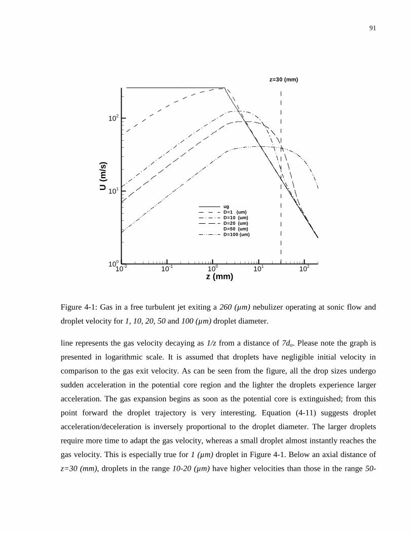
91

Figure 4-1: Gas in a free turbulent jet exiting a 260 (µm) nebulizer operating at sonic flow and

droplet velocity for 1, 10, 20, 50 and 100 (µm) droplet diameter.

line represents the gas velocity decaying as 1/z from a distance of 7do. Please note the graph is

presented in logarithmic scale. It is assumed that droplets have negligible initial velocity in

comparison to the gas exit velocity. As can be seen from the figure, all the drop sizes undergo

sudden acceleration in the potential core region and the lighter the droplets experience larger

acceleration. The gas expansion begins as soon as the potential core is extinguished; from this

point forward the droplet trajectory is very interesting. Equation (4-11) suggests droplet

acceleration/deceleration is inversely proportional to the droplet diameter. The larger droplets

require more time to adapt the gas velocity, whereas a small droplet almost instantly reaches the

gas velocity. This is especially true for 1 (µm) droplet in Figure 4-1. Below an axial distance of

z=30 (mm), droplets in the range 10-20 (µm) have higher velocities than those in the range 50-

z (mm)

U(m

/s)

10-2

10-1

100

101

10210

0

101

102

ug

D=1 (um)

D=10 (um)

D=20 (um)

D=50 (um)

D=100 (um)

z=30 (mm)

92

100 (µm) due to their original larger acceleration in the potential core region, therefore below

this location we’ll have a cloud of fast moving droplets within a cloud of slow moving particles.

For downstream locations beyond 30 (mm) this trend is reversed, because 10-20 (µm) droplets

have already adapted the gas velocity, but larger droplets require more time, therefore we’ll have

a cloud of large droplets passing through a cloud of relatively slow moving droplets. 10 and 20

(µm) droplets require 40 and 70 (mm) to reach the gas velocity, respectively, while 50 and 100

(µm) droplets must travel over 200 (mm) to creep up to the gas velocity. The simplified model

presented here is valid for diluted spray where the drop number density is small, in other words

when the gas phase in not disrupted by the presence of the droplets. Please note that in our model

we have neglected the spatial dispersion and evaporation, nevertheless the model help us

understand some basic physical processes occurs during aerosol transportation.

Aerosol Velocity Modeling 4.2

In the spray jet of pneumatic nebulizers, the momentum is exchanged between the gas and liquid

phases. For instance as Sharp (80) explains, a 1 (l/min) flow of argon at 293 (K) and 1.014×105

(Pa) is equivalent to a mass flow rate of 1.66 (g/min) that would typically nebulize an equivalent

mass of liquid, in other words a mass flow ratio of approximately one. Introducing liquid thus

doubles the mass flow rate and to conserve momentum, the mean velocity of the seeded gas must

drop to one half of its non-seeded value from Equation (4-4). Sharp (80) also adds:” Although

the presence of liquid reduces the gas momentum, it does not necessarily reduce the entrainment.

Moving particles entrain fluid in their wake and in dense clouds may cause the fluid to move at

the mean particulate velocity.”

Equation (4-4) and the simplified model presented in the previous section are valid only when

the spray is diluted, in other words when the liquid mass flow rate is small in comparison to that

of the gas and provided that all the droplets travel along the nebulizer axis. For large liquid to gas

flow ratios, the dynamics of particle and gas motion requires detailed modeling that includes the

transfer of momentum between the two phases and effects of droplet dispersion. Hence not only

the actual gas velocity would be different but also the resultant droplet velocities would deviate

from the model. Our aim here is to present simple correlations for estimating aerosol velocity

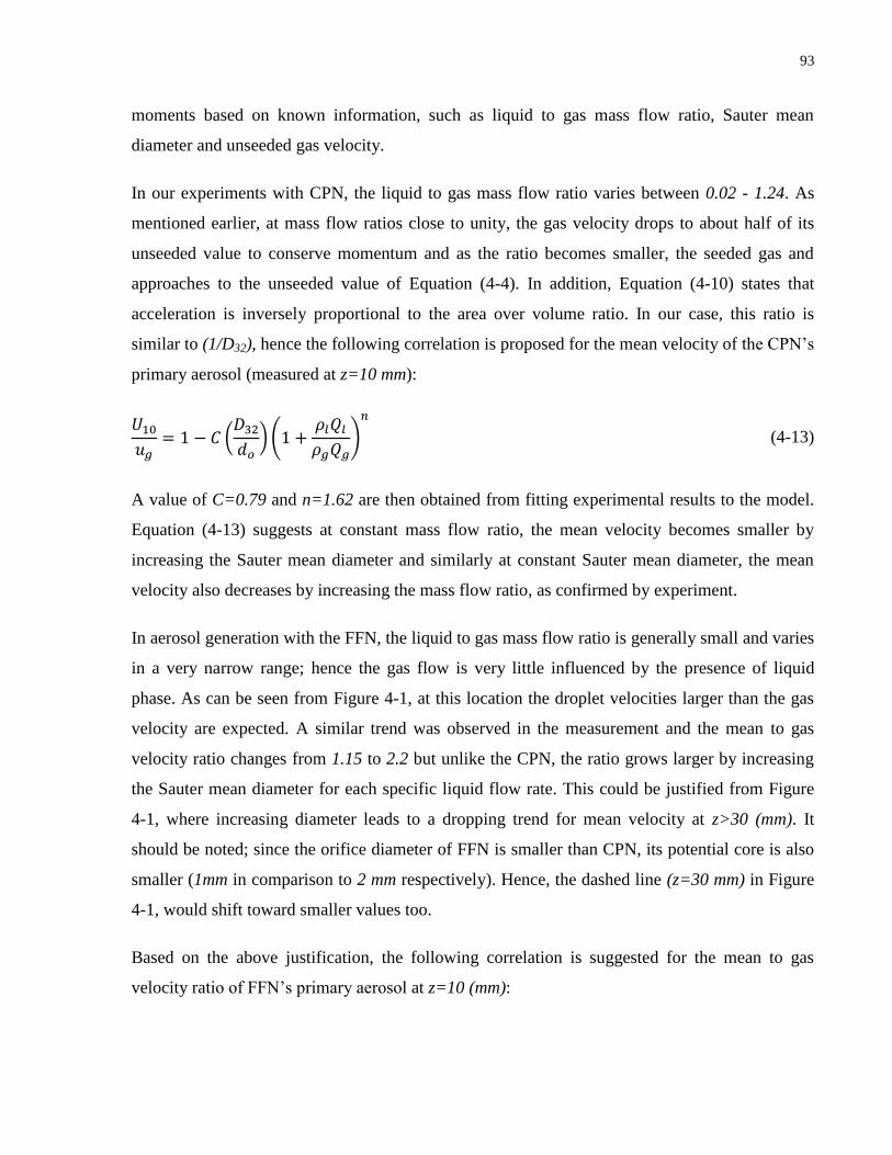
93

moments based on known information, such as liquid to gas mass flow ratio, Sauter mean

diameter and unseeded gas velocity.

In our experiments with CPN, the liquid to gas mass flow ratio varies between 0.02 - 1.24. As

mentioned earlier, at mass flow ratios close to unity, the gas velocity drops to about half of its

unseeded value to conserve momentum and as the ratio becomes smaller, the seeded gas and

approaches to the unseeded value of Equation (4-4). In addition, Equation (4-10) states that

acceleration is inversely proportional to the area over volume ratio. In our case, this ratio is

similar to (1/D32), hence the following correlation is proposed for the mean velocity of the CPN’s

primary aerosol (measured at z=10 mm):

( ) (

)

(4-13)

A value of C=0.79 and n=1.62 are then obtained from fitting experimental results to the model.

Equation (4-13) suggests at constant mass flow ratio, the mean velocity becomes smaller by

increasing the Sauter mean diameter and similarly at constant Sauter mean diameter, the mean

velocity also decreases by increasing the mass flow ratio, as confirmed by experiment.

In aerosol generation with the FFN, the liquid to gas mass flow ratio is generally small and varies

in a very narrow range; hence the gas flow is very little influenced by the presence of liquid

phase. As can be seen from Figure 4-1, at this location the droplet velocities larger than the gas

velocity are expected. A similar trend was observed in the measurement and the mean to gas

velocity ratio changes from 1.15 to 2.2 but unlike the CPN, the ratio grows larger by increasing

the Sauter mean diameter for each specific liquid flow rate. This could be justified from Figure

4-1, where increasing diameter leads to a dropping trend for mean velocity at z>30 (mm). It

should be noted; since the orifice diameter of FFN is smaller than CPN, its potential core is also

smaller (1mm in comparison to 2 mm respectively). Hence, the dashed line (z=30 mm) in Figure

4-1, would shift toward smaller values too.

Based on the above justification, the following correlation is suggested for the mean to gas

velocity ratio of FFN’s primary aerosol at z=10 (mm):

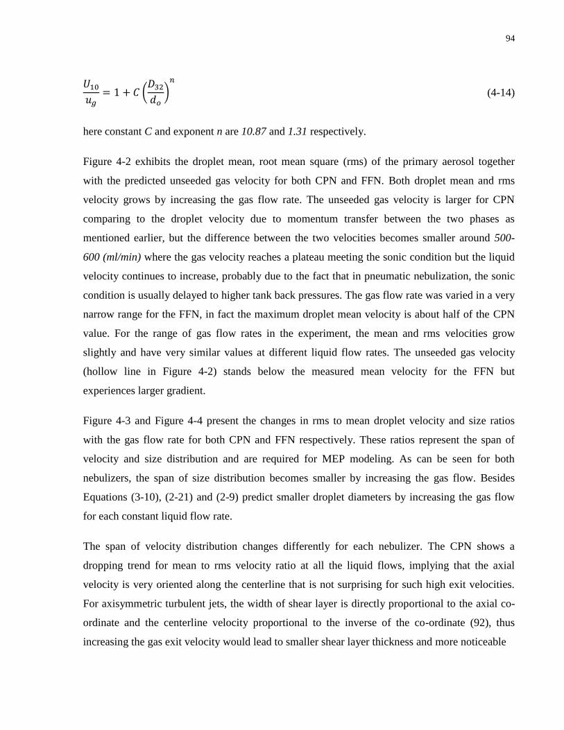
94

( )

(4-14)

here constant C and exponent n are 10.87 and 1.31 respectively.

Figure 4-2 exhibits the droplet mean, root mean square (rms) of the primary aerosol together

with the predicted unseeded gas velocity for both CPN and FFN. Both droplet mean and rms

velocity grows by increasing the gas flow rate. The unseeded gas velocity is larger for CPN

comparing to the droplet velocity due to momentum transfer between the two phases as

mentioned earlier, but the difference between the two velocities becomes smaller around 500-

600 (ml/min) where the gas velocity reaches a plateau meeting the sonic condition but the liquid

velocity continues to increase, probably due to the fact that in pneumatic nebulization, the sonic

condition is usually delayed to higher tank back pressures. The gas flow rate was varied in a very

narrow range for the FFN, in fact the maximum droplet mean velocity is about half of the CPN

value. For the range of gas flow rates in the experiment, the mean and rms velocities grow

slightly and have very similar values at different liquid flow rates. The unseeded gas velocity

(hollow line in Figure 4-2) stands below the measured mean velocity for the FFN but

experiences larger gradient.

Figure 4-3 and Figure 4-4 present the changes in rms to mean droplet velocity and size ratios

with the gas flow rate for both CPN and FFN respectively. These ratios represent the span of

velocity and size distribution and are required for MEP modeling. As can be seen for both

nebulizers, the span of size distribution becomes smaller by increasing the gas flow. Besides

Equations (3-10), (2-21) and (2-9) predict smaller droplet diameters by increasing the gas flow

for each constant liquid flow rate.

The span of velocity distribution changes differently for each nebulizer. The CPN shows a

dropping trend for mean to rms velocity ratio at all the liquid flows, implying that the axial

velocity is very oriented along the centerline that is not surprising for such high exit velocities.

For axisymmetric turbulent jets, the width of shear layer is directly proportional to the axial co-

ordinate and the centerline velocity proportional to the inverse of the co-ordinate (92), thus

increasing the gas exit velocity would lead to smaller shear layer thickness and more noticeable

95

(a)

(b)

Figure 4-2: Droplet Mean and Root Mean Square (rms) speed and unseeded gas velocity versus

gas flow rate, measured at z=10 (mm) for (a) CPN and (b) FFN.

0

10

20

30

40

50

60

70

200 300 400 500 600 700 800

U10, U

rms,

ug (

m/s

)

Qg (ml/min)

Velocity curves for CPN

U10, Ql=1 (µl/s)

Urms, Ql=1 (µl/s)

U10, Ql=5 (µl/s)

Urms, Ql=5 (µl/s)

U10, Ql=10 (µl/s)

Urms, Ql=10 (µl/s)

ug

Sonic condition

0

5

10

15

20

25

30

140 160 180 200 220

U1

0, U

rms,

ug (

m/s

)

Qg (ml/min)

Velocity curves for FFN

U10, Ql=0.1 (µl/s)

Urms, Ql=0.1 (µl/s)

U10, Ql=0.2 (µl/s)

Urms, Ql=0.2 (µl/s)

U10, Ql=0.4 (µl/s)

Urms, Ql=0.4 (µl/s)

U10, Ql=0.6 (µl/s)

Urms, Ql=0.6 (µl/s)

ug

96

(a)

(b)

Figure 4-3: Span of (a) velocity and (b) size distribution measured at z=10 (mm) for CPN.

0.3

0.32

0.34

0.36

0.38

0.4

0.42

0.44

0.46

0.48

0 200 400 600 800 1000

Urm

s/U

10

Qg (ml/min)

Velocity distribution span for CPN

Ql= 1 (µl/s)

Ql= 5 (µl/s)

Ql= 10 (µl/s)

0.3

0.35

0.4

0.45

0.5

0.55

0.6

0.65

0.7

0.75

0 200 400 600 800 1000

Drm

s/D

10

Qg (ml/min)

Size distribution span for CPN

Ql= 1 (µl/s)

Ql= 5 (µl/s)

Ql= 10 (µl/s)

97

(a)

(b)

Figure 4-4: Span of (a) velocity and (b) size distribution measured at z=10 (mm) for FFN.

0.3

0.32

0.34

0.36

0.38

0.4

0.42

0.44

0.46

0.48

0.5

100 150 200 250

Urm

s/U

10

Qg (ml/min)

Velocity distribution span for FFN

Ql=0.1 (µl/s)

Ql=0.2 (µl/s)

Ql=0.4 (µl/s)

Ql=0.6 (µl/s)

0.45

0.5

0.55

0.6

0.65

0.7

100 150 200 250

Drm

s/D

10

Qg (sccm)

Size distribution span for FFN

Ql=0.1 (µl/s)

Ql=0.2 (µl/s)

Ql=0.4 (µl/s)

Ql=0.6 (µl/s)

98

aerosol confinement. As a result the droplet radial dispersion would be smaller and more uniform

velocity droplets pass the measuring probe of the PDPA. This trend is not observed for the FFN,

perhaps because gas and droplet velocities are smaller and change in a narrower range compared

to the CPN. The span of velocity distribution grows larger by increasing gas flow rate at Ql=0.1-

0.2 (µl/s) but remains constant or have slight variation at Ql=0.4-0.6 (µl/s). In summary we may

say that finer aerosols at higher velocities with narrower size and velocity distribution are

resulted from increasing the gas flow rate for the CPN. Doing so for the FFN would result in a

finer and narrower size distribution with droplets traveling at slightly higher velocities and

increased velocity dispersion. The axial and radial variations of the mean and rms velocities are

given in Appendix D. These plots together with the size characteristics moments of Appendix C

can be used in MEP modeling (Chapter 5) to generate size and velocity distributions at any

desired location such as the spray fringe or centerline.

Contribution 4.3

Droplets with wide ranges of velocities produce emission and mass spectrometric signals at

different locations in the plasma, leading to reduced sensitivity and signal fluctuations. Besides,

high velocity droplets may not have enough residence time for complete evaporation. Therefore,

controlling the aerosol velocity in ICP-MS is of significant importance. In this chapter, first, the

axial and radial profiles of the centerline velocity for a turbulent free jet were presented and then

the response of different droplet sizes in the flow was studied. It was found that below some

axial distance, the aerosol stream consists of fast and small cloud of droplets moving in a cloud

of slow and large droplets but this would be reversed further downstream where small drops

adapt the gas velocity faster than large droplets. As discussed in the chapter, increasing either the

liquid to gas mass flow ratio or the Sauter mean diameter for CPN reduces the mean aerosol to

gas velocity ratio because of the momentum transfer between the two phases. A correlation was

proposed for the velocity ratio as a function of mass flow ratio and Sauter mean diameter in

Equation (4-13). In microsample nebulization with FFN, since the liquid flow is negligible in

comparison to the gas flow, as discussed in the single droplet model, the mean velocity becomes

larger by increasing the droplet size. Equation (4-14) was proposed to account for this

observation.

99

Chapter 5 Maximum Entropy Principle - Application on Aerosol Size and

Velocity Modeling

The Need for Statistical Measures and Maximum Entropy 5.1Principle

The primary aerosol size of the CPN and FFN was characterized in Chapters 2 and 3

respectively, and the velocity characterization was presented in Chapter 4 where some

correlations was either modified or proposed. The characteristic moments of size and velocity

although contain important information, only represent aerosol characteristics macroscopically

rather than the detailed space of size and velocity. Nonetheless the atomization is in general the

process of fragmenting liquid bulk into multiplicity of droplets with different sizes and

velocities. In fact, in many industrial applications like automotive paint sprays, waste

incineration, pharmaceutical/medical drug administration (93) and agricultural aviation for crop

spray (94) the drop size distribution must have a particular form (narrow, wide, few large drops,

few small drops, etc.) for optimal operation. In atomic and mass spectrometry for instance, the

nebulizer transport efficiency is of crucial importance; that is the fraction of aerosol volume

containing sub 10 (µm) droplets (Refer to Figure 3-11 to Figure 3-14). For given flow conditions,

if two nebulizers have the same Sauter mean diameter for example, the one which has higher

transport efficiency is preferred. On the other hand as mentioned in the previous chapter, if the

aerosol droplets travel fast, the particle residence time in the plasma would not be adequate for

complete vaporization even if the entire aerosol contains sub 10 (µm) droplets. Therefore, as far

as sample introduction in ICP-MS is concerned, some aspects of the aerosol generation require

detailed information on the entire size and velocity space that may not be reflected through

characteristic moments alone.

Although the droplet distribution space can be easily measured by Phase Doppler Anemometry,

the stochastic nature of sprays has drastically restricted the development of mathematical or

numerical modeling of sprays. In fact deterministic methods such as instability analysis up to this

point are not advanced enough and generally incapable of including all the mechanism involved

100

in a simple liquid atomization process. Consequently, all they could offer may not exceed more

than single droplet diameters under very simplified conditions at best. In the absence of such

comprehensive models, many different empirical distributions like Rosin-Rammler (95),

Nukiyama-Tanasawa (51), Lognormal (96), upper-limit (97), Log-hyperbolic (98), etc. have

been proposed, none which offers universal prediction and are only valid in the range they are

proposed and tested. Furthermore, among these distributions only Log-hyperbolic has been

expanded to present joint size and velocity distribution while others can only model size

distribution. Besides, the empirical distributions bring little physical understanding of the

process and even worse they are not founded on a mathematical ground. Thus, all of these

correlations could be considered more or less as curve fitting methods for covering a range of

experimental data. The study of these empirical distributions is beyond the scope of this study;

nonetheless they are given in Appendix E for comparison.

Although CFD has been widely used as a powerful tool in many different applications for

modeling spray dynamics, simulating all the details of the primary atomization and liquid

disintegration in Eulerian frame of reference is very time consuming and has considerable

numerical cost. The alternative practice is to use some statistical measure of primary aerosol

space as input and then study the secondary effects such as breakup, collision, coalescence,

evaporation, impaction, etc. in a coupled Eulerian-Lagrangian frame of reference.

Therefore, from practical point of view, it would be very beneficial to have some statistical

measures of the primary aerosol, i.e. the detailed size and velocity space, with as little

information possible and preferably based on the measured characteristic moments.

The maximum entropy principle (MEP) is a promising approach toward the prediction of the

spray distribution which has a mathematical foundation. The principle was developed by Jaynes

(99) based on Shannon’s entropy concept (100) which is a measure of uncertainty of a system

subjected to some prescribed constraints. Shannon originally defined this entropy to study

communication of information through a noisy channel. Jaynes (99) showed that based on

Shannon’s approach all of the formulae of statistical mechanics could be easily derived.

Nevertheless he stated that the foundation of this definition of entropy is quite independent from

statistical mechanics. Since then Shannon entropy and Jaynes’ maximum entropy principles have

101

been successfully employed in many different disciplines of natural and social sciences such as

transportation, population, brand-switching in marketing and vote-switching in elections, finance

insurance and marketing, image reconstruction, pattern recognition, operation research and

engineering, biological medical and technological problems, non-parametric density estimation

(101) to just name a few.

MEP Formulation 5.2

Atomization is a highly nonlinear and stochastic process and the deterministic methods fail

miserably in predicting the aerosol space. Alternatively, MEP can present the least biased and the

most objective solution even if only small pieces of information about the spray are known

beforehand.

The pioneering application of MEP for spray modeling first appeared in the works of Sellens

(102), Sellens and Brzustowski (103) and (104), and Li and Tankin (105) and (106)

independently. All these tasks investigated the problem of distributing droplets in a size and

velocity space when discrete information was given or known from experimental measurement.

Consider a size and velocity space as shown in Figure 5-1. The droplets are assumed to be

distributed in different classes of normalized size and velocity respectively while the space is

equally segmented to avoid any biased analysis. At this point the reference diameter (Dref) and

velocity (Uref) are not determined but will be specified later. In this figure, the number of

droplets in a particular class of normalized size and velocity is given by ΔNij and the total

number of droplets is Ntot=ΣΣ ΔNij, thus the probability of finding a droplet in a particular class

of normalized size and velocity is Pij= ΔNij/Ntot and the corresponding probability per unit

normalized size and velocity class will be fij.

The trivial constraint for any distribution in this space is that the summation of all the

probabilities must be unity (normalization constraint):

∑∑

∑∑

(5-1)

102

Figure 5-1: Size and velocity space and probability distribution function of aerosol

Nevertheless, the aerosol might be subjected to some other constraints which are often presented

in terms of some characteristic moments (γk) either measured from experiment or known from

theoretical analysis.

∑∑ (

)

∑∑ (

)

(5-2)

The constraints (gk’s) in Equation (5-2) are conventionally derived from first principles or

conservation laws acting on the aerosol. However this is not a necessary condition for the given

constraints and any single or joint function of size and velocity can be used as long as its value is

known beforehand.

If ΔD* and ΔU

* are small, Equations (1-5) and (2-5) can be presented in continuous form:

103

∫ ∫

(5-3)

∫ ∫

( ) (5-4)

There are many possible distributions in the size and velocity space that satisfy the normalization

constraint (5-3) and the additional prescribed information (5-4), however the maximum entropy

principle states out of these possible distributions, the one that maximizes the Shannon entropy is

the least biased and the most objective distribution for the prescribed information. The Shannon

entropy is defined as:

∫ ∫

( ) (5-5)

The derivation of Shannon entropy is beyond the scope of this task but presented in Appendix F.

The method of Lagrangian multipliers is employed to find the least biased distribution:

( )

∑

(5-6)

∫ ∫ ( ( ) ∑

( ))

(5-7)

The integral Equation (5-7) is always true if the integrand is identically zero, thus:

( [∑ ( )

]) (5-8)

The unknown coefficients must be found by solving the integral Equations (5-3) and (5-4) with

the probability distribution function given in Equation (5-8). The lower limit of integration for

104

both the minimum diameter and velocity can be set equal to zero although it’s possible to assume

a non-zero value for minimum size since generating a zero size droplet is physically impractical.

The upper limit of the integration is infinity but for numerical calculations some finite value

must be taken. Van Der Geld and Vermeer (107) have proven the boundaries of integration may

shift the the probability distribution but the question of correct integration limits has never been

addressed in the literature. In this task, the upper limit of integration is taken from the PDPA

optical restrictions, which is Dmax=120 (µm) and Umax=100 (m/s) respectively.

Once the entropy function is determined, the size and velocity distributions are obtained by

taking proper integration:

∫

(5-9)

∫

(5-10)

Number or Volume Based Probability Distribution Function? 5.3

Since the employment of MEP in the field of atomization and sprays, two separate MEP

implementations with a fundamental difference can be recognized in the literature. One is the

Sellens and Brzusowski’s approach and the other is Li and Tankin’s. Before presenting the MEP

modeling, the two approaches must be discussed.

Sellens (102) and Sellens and Brzustowski (103) and (104) used a size and velocity space as

shown in Figure 5-2 to study the joint size and velocity distribution of a pressure swirl atomizer.

The author used a control volume surrounding the sheet breakup plane (Figure 5-2) and

expressed the physical laws acting on the control volume as the conservation constraints of mass,

surface energy, momentum and kinetic energy:

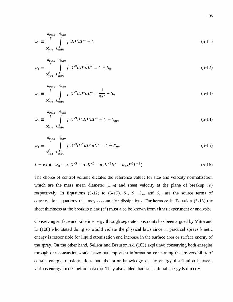
105

∫ ∫

(5-11)

∫ ∫

(5-12)

∫ ∫

(5-13)

∫ ∫

(5-14)

∫ ∫

(5-15)

(

) (5-16)

The choice of control volume dictates the reference values for size and velocity normalization

which are the mass mean diameter (D30) and sheet velocity at the plane of breakup (V)

respectively. In Equations (5-12) to (5-15), Sm, Ss, Smv and Ske are the source terms of

conservation equations that may account for dissipations. Furthermore in Equation (5-13) the

sheet thickness at the breakup plane (η*) must also be known from either experiment or analysis.

Conserving surface and kinetic energy through separate constraints has been argued by Mitra and

Li (108) who stated doing so would violate the physical laws since in practical sprays kinetic

energy is responsible for liquid atomization and increase in the surface area or surface energy of

the spray. On the other hand, Sellens and Brzustowski (103) explained conserving both energies

through one constraint would leave out important information concerning the irreversibility of

certain energy transformations and the prior knowledge of the energy distribution between

various energy modes before breakup. They also added that translational energy is directly

106

Figure 5-2: Sellens and Brzustowski’s control volume for MEP modeling.

transformed into surface energy by sheet stretching and drop drag formation but the reverse

transformation from surface to direct kinetic energy is generally not possible and hence separate

constraint for each mode of energy must be considered.

Sellens’ (102) and Sellens and Brzustowski’s models (103) and (104) are in general agreement

with empirical correlations and particularly Rosin-Rammler distribution except that the

distribution function (Equation 16-5) shows some non-zero population for zero size droplets

which is not supported by experiment. Sellens (109) and (110) later resolved the issue by

introducing a new constraint which he called the “partition of surface energy”. As Sellens

explains the unphysical behavior is due to a deficiency in the conservation moments because the

lowest order moment of size is of second order and the small size droplets have little contribution

to the values of the size moments (Equation 5-12 and 5-13). Sellens added that in limiting the

number of very small drops, the physical process at work is a limitation of the concentration of

surface energy. With fixed values of surface tension, flow velocities, etc. it is unlikely that

sufficient deformation energy will be expanded on a given element of mass to reduce the drop

Control Volume

GasLiquid

Sheet Breakup

Drops

107

size beyond a certain point. Thus the amount of deformation energy that a small element of mass

can absorb must be limited or, in other words, the surface to volume ratio of the drops in the

spray imposes a constraint:

∫ ∫

(5-17)

here Kp expresses the strength of the partition constraint which is equal to the nameless

characteristic moment (D-10) that was introduced by Equation (2-23). If the new constraint is

added to set of Equations (5-11) to (5-15) the resulted distribution function will be:

(

) (5-18)

In 1987 Li and Tankin (105) derived a size distribution through the concept of information

theory and maximum entropy principle and showed the resultant distribution is a special case of

Nukiyama and Tanasawa distribution (51). In this study, Li and Tankin were only interested in

size distribution, therefore the velocity was not included in the solution space. Furthermore,

instead of using size classes, the space was divided by volume classes.

∫

(5-19)

∫

(5-20)

where fv and V* are the volume distribution function and the normalized droplet volume

respectively. Li and Tankin stated that since the probability of finding a droplet in a particular

class of size is essentially the same as probability of finding it in the corresponding volume, thus

Equations (5-19) and (5-20) can be rearranged as:

*

+ *

+ (5-21)

108

( ) (

) ( ) (5-22)

∫

(5-23)

∫

(5-24)

(

) (5-25)

Li and Tankin (70), (106) and (111) developed their model to include the velocity by including

the the momentum and kinetic energy constraints, Nevertheless a single constraint is considered

for the total energy (surface and kinetic energy). In contrast to Sellens and Brzustowski (103)

and (104) the control volume was assumed to be extended from the orifice exit to the plane of

breakup. This choice of control volume dictates D30 and capillary velocity (Ucap) for

normalization of size and velocity respectively as shown in Figure 5-3.

∫ ∫

(5-26)

∫ ∫

(5-27)

∫ ∫

(5-28)

∫ ∫

( (

) ) (5-29)

109

(

( (

) )) (5-30)

An interesting feature of Equation (5-30) is that the probability distribution approaches to zero as

the drop diameter decreases; hence there is no need to prescribe an additional constraint like the

partition of surface energy in Equation (5-17). However Dumouchel (112) believes that this

problem was avoided in Lin and Tankin’s papers (105), (106) and (70) due to mathematical

manipulation in Equation (5-22) which indicates that the number based drop size distribution is

proportional to the square of the drop diameter.

In the absence of any priori information, the least biased distribution must be the uniform one.

This is the case for Sellens and Burzustowski’ number based distribution (Equations 5-11 and 5-

16) when constraints (5-12) to (5-15) are not prescribed. But with normalization constant alone,

Li and Tankin’s approach leads to a constant f’(V*) or according to Equation (5-22) a number

based size distribution that is a function of D*2

. Nonetheless such hypothesis has never been

supported by any experimental evidence or by theoretical study. Dumouchel (112) concluded, as

far as MEP is concerned a change of variable introduces supplementary information and must be

avoided. In Cousin et al.’s excellent study (113), the issue of number and volume distribution

was finally addressed. The authors showed that the number and volume based distribution must

be consistent, meaning that entropy maximization with either size or volume must result in the

same size and volume distributions. Besides it was shown a number based size distribution can

be derived by maximizing Shannon entropy. On the other hand, a correct volume based

distribution can only be calculated if a priori distribution that contains the information related to

the shape of droplets is considered to maximize Bayesian entropy which is the more general

form of Shannon entropy (113). Refer to Appendix G for the definition Bayesian entropy and its

relation with Shannon entropy.

Taking Sellens formulation (Equations 5-11 to 5-18) to find the number based distribution, the

corresponding volume based distribution can be easily calculated by:

( )

(

) ( ) (5-31)

110

Figure 5-3: Li and Tankin’s control volume for MEP modeling.

Global and Local Implementation of MEP 5.4

The classical control volume approaches of Sellens and Brzustowski (103) and Li and Tankin

(106), (111) have considered the conservation laws between two plains, the known upstream

plane and the droplet plane. In deriving conservation of mass constraints in Equations (5-12), (5-

24) and (5-27) it was assumed that the liquid flow rate is the same as the rate of droplet masses

passing the PDPA probe are comparable. However, we have observed a considerable mismatch

between these two parameters which is also supported by Li et al.’s study (114). The authors

attributed this problem to two possible factors: (1) defining the optical probe measurement cross

section and (2) high rate of data rejection. On the other hand, the control volume approach

requires the PDPA measurements to cover the entire spray cross section (111) but the probe area

of the order of 10-2

(mm2) and the spray cross section of 10

2 (mm

2) at the downstream location

makes this task nearly impractical.

The other problem of the control volume approach (global implementation) of MEP is that, the

sheet thickness and velocity must be calculated for Sellens and Brzustowski’s model. Lefebvre

(50) criticized this model stating that although the approach is elegant, such quantities are not

Control Volume

GasLiquid

Sheet BreakupDrops

111

easily measured. In fact, Rizk and Lefebvre (23) have shown the film thickness can change

significantly with the flow parameters (23). From this perspective, Li and Tankin’s control

volume extended from the orifice exit is preferable because it links the breakup plane to the

known upstream conditions. However, such control volume requires careful estimation of the

source terms in Equations (5-27) to (5-29) since the effect of downstream gas and liquid

interaction between the two planes can be quite considerable. Moreover and to the best of the

author’s knowledge, there is no study in the literature that has focused on the details of

prefilming, sheet breakup or any photographic measurement for ICP nebulizers. A comparison of

Figure 1-4 with Figure 5-2 and Figure 5-3 of pressure atomizers reveals that the mechanism of

liquid disintegration is very different which makes adapting an appropriate control volume very

difficult.

Ahmadi and Sellens (115) state that the MEP does not have to be necessarily applied on the

entire spray cross section and added that in general the principle holds true for any local control

volume at any particular time and location. This would mean the MEP application is quite

independent of the choice of control volume and is not merely derived from conservation laws.

In other words, if the mass, surface energy, momentum, kinetic energy and partition of surface

energy are important characteristics of the aerosol stream as the whole, they are equally

important description of the local state of spray. This feature of MEP is of particular importance.

Consider the case that you are only interested in the local distribution of size and velocity at a

particular point in the spray, the global implementation of MEP as in Sellens and Brzustowski’s

model (Equations 5-11 to 5-15) or Li and Tankin’s model (Equations 5-26 to 5-30) is incapable

of offering a solution, because they represent the entire spray plane. Ahmadi and Sellens,

findings have proven that the MEP can be regarded as a tool for statistical inference of the spray

that is not restricted to the conservation laws. Since then a number of MEP-based size

distribution such as (112), (117), (118), (119), (120) and (113) have exploited this approach for

aerosol modeling.

In direct injection of droplets by FFN for example, the fate of droplets traveling along the

nebulizer axis is important rather than the entire spray cross section because these droplets are

more likely to reach the plasma channel (9). In Sample introduction with a conventional CPN,

the small drops are found along the axis while larger ones formed at the fringes of the spray and

112

will be probably removed by the spray chamber. Since we are interested to have a statistical

measure of aerosol along the centerline of the nebulizers, the principle has to be implemented

locally rather than globally. Besides, as both size and velocity distribution are important in ICP-

MS our local MEP implementation must also include the velocity subspace.

Before local MEP formulation is presented, it’s worth mentioning again that the global

implementation of MEP dictates the reference values of size and velocity. In contrast, the local

implementation allows us to choose any arbitrary reference values for parameter normalization.

As mentioned in the previous chapters, the measured droplet velocities are orders of magnitude

larger than the liquid velocity in the capillary. Thus Li and Tankin’s normalization with capillary

velocity does not seem appropriate. On the other hand, the film velocity of Sellens and

Brzustowski’s model cannot be easily measured. We have chosen the local unseeded gas

velocity, ug(z) for velocity normalization because its value is of the same order as the measured

droplet velocity which makes it more relevant for normalization. The value of gas velocity can

be calculated from Chapter 4 and the relations given within. In addition the droplet size is

normalized by mass mean diameter D30 as the other two models.

∫ ∫

(5-32)

∫ ∫

(5-33)

∫ ∫

(5-34)

∫ ∫

(5-35)

113

∫ ∫

(5-36)

∫ ∫

(5-37)

(

) (5-38)

( ) (5-39)

As can be noticed from Equations (5-32) to (5-37) the values of constraint are also given except

for the joint momentum and kinetic energy source terms. The values of D30/D20 and D30/D-10 can

be extracted from Chapters 2 and 3 for CPN and FFN respectively. Equations (5-35) and (5-36)

can be simplified to U10/ug(z) and (U10/ug(z))2 + (Urms/ug(z))

2 if spray monodispersity exists in

either size, velocity or both (116). In our study depending on the degree of spray polydispersity,

the momentum and kinetic energy constraints are up to 1.5 and 2.5 folds their monodisprse

values respectively.

Numerical Solution 5.5

After finding the closed form of probability distribution function through method of Lagrangian

multipliers, the unknown coefficients must be determined by solving the integral Equations (5-

32) to (5-37). Li (121) has proven not only a solution to system of equations exists but it is

unique as well, providing that the constraint values are positive, i.e. Γk>0.

Unfortunately the sets of equations are highly nonlinear that makes finding analytical solution

rather impossible. In the present study, we have used the iterative Newton-Raphson method to

find the unknown coefficients. Iteration begins with an initial guess for the coefficients which in

our case are set to zero. The Jacobian matrix is first constructed by differentiating Equations (5-

32) to (5-37) and distribution function (5-38) and then the matrices of constants and Jacobian are

evaluated for the given initial guess.

114

[

]

⏟

[

]

⏟

[

]

⏟

(5-40)

The increment matrix (Δα) is therefore:

(5-41)

The inverse Jacobian matrix (J-1

) is calculated through Gauss-Jordan elimination method. Once

the increment matrix is obtained, the new coefficients are calculated.

(5-42)

The procedure is repeated with new coefficients until the constant matrix converges to zero, or in

other words:

(5-43)

where epsilon is set to a small value (10-10

). It’s important to keep epsilon small because the

equations are in exponential form and double integration is also involved. Therefore a small

imbalance may cause severe numerical error. The convergence of the numerical scheme depends

on the initial guess and also the stiffness of the Jacobian matrix. A second order Newton-

Raphson method has been proposed in (122) to overcome the stability and restrict requirement

on the initial guess. In our study, the local implementation of MEP and velocity normalization

with the local gas velocity, ug(z), reduces the stiffness of the Jacobian matrix significantly and

ensures the numerical convergence with fewer than 30 iterations at most with the first order

Newton-Raphson method shown by Equations (40-5) to (42-5).

115

MEP Results and Discussion 5.6

Figure 5-4 demonstrates the result of size distribution from the coupled MEP model for two

representative cases of Ql=5 (µl/s), Qg=500 (ml/min) and Ql=0.1 (µl/s), Qg=150 (ml/min)

sprayed with CPN and FFN respectively. As can be seen, the standard deviation (STD) of the

experimental results are small (maximum of 8 and 12% for CPN and FFN respectively) modeled

size distributions are in general agreement with experiment. The Skewness of distribution and

the location of most probable diameter are correctly predicted, although probability value

exhibits some underestimation. Besides span of distribution covers the experiment and the

population of very fine and large droplet approaches to zero at the end tail of the distributions as

producing such droplet sizes are not physically probable.

The majority of studies on MEP modeling have focused mainly on the size distribution. The

velocity distribution has received little or no attention even when the joint size and velocity pdf

are employed. For instance, in Sellens and Brzutowski’s paper (103) although momentum and

kinetic energy moments are prescribed, the velocity distribution is not reported and many other

studies the velocity distributions are presented without comparison to the experiment (104),

(109), (106) and (111).

Figure 5-5 presents the velocity distributions for the same cases of Figure 5-4. Several

deficiencies can be noticed from the figure. First, the end tails population does not agree with

experiment; in the experiment the population of small and large velocity converges to zero while

the model predicts some non-zero population for these drops. Second, the span of the distribution

does not show good agreement and, third the location and population of the most probable

velocity is largely different, particularly for the FFN. The behavior of our results resembles those

of Kim et al.’s study (123), one of the few studies that compared the predicted velocity

distribution with experiment (Refer to Figures 7, 9 and 11 in (123)). This problem had also come

to the attention of Bhatia and Durst (98), (124) and (125), where the authors concluded that the

available MEP models fail to predict the overall pdf correctly and proposed an alternative log-

hyperbolic pdf and added that their model is “the best choice among both one- and two-

dimensional distributions”. Nonetheless the log-hyperbolic model requires extensive numerical

calculation which is not practical, besides the model is justified by purely empirical means.

116

(a) CPN

D*

dN

*/d

D*

0 1 2 3 4 5 6 70

0.5

1

1.5

Experiment

Original 6 constraint model

Replaced constraint model

Added constraint model

117

(b) FFN

Figure 5-4: Primary aerosol size distribution measured at z=10 (mm) for (a) Ql=5 (µl/s) at

Qg=500 (ml/min), D30=16.2 (µm) and (b) Ql=0.1 (µl/s) at Qg=150 (ml/min), D30=14.4 (µm).

Error bars represent standard deviation.

We also believe nullifying all the past efforts in MEP modeling does not seem to be fair either.

For example, one could equally argue that the log-hyperbolic may only apply to strongly

monomodal distributions while bimodal distributions are successfully modeled by MEP (126)

and (127). Besides, as far as MEP is concerned the resultant distribution is the most objective

and the least biased distribution for the prescribed information. Kapur (101) states MEP may

D*

dN

*/d

D*

0 2 4 6 80

0.5

1

1.5

Experiment

Original 6 constraint model

Replaced constraint model

Added constraint model

118

necessarily lead to correct (physical here) solution, in such situation more information should be

specified, i.e., additional constraints should be used or given in a different form.

As may be noticed from Equations (5-32) to (5-37), the velocity information is only given

through joint moments of momentum and kinetic energy while the size information is prescribed

in both formats, first through single moments (conservation of mass, surface energy and partition

of the surface energy) and second in the joint moments. Thus, one possible solution might be

substituting the joint moments. Since the simplest distribution is the Gaussian distribution that

needs only single moments of mean and rms, we prescribed the same information to the MEP

model. This would imply the following substitution in the equations:

∫ ∫

( )

(5-44)

∫ ∫

( ( )

)

( ( )

)

( ( )

)

(5-45)

(

) (5-46)

but the other equations will remain untouched. We will call this model the replaced constraint

model. The alternative approach would be prescribing the two moments to the seat of constraints

so that like size, velocity information is also given in both single and joint formats (added

constraint model). The new constraints and the revised distribution function would then be:

∫ ∫

( )

(5-47)

∫ ∫

( ( )

)

( ( )

)

(5-48)

(

) (5-49)

119

Figure 5-4 shows that adding or replacing velocity moments do not vary the size distribution

considerably as mentioned in (116). As can be seen the applied changes only dislocated the most

probable size and its probability to a very small degree. Thus we may draw the conclusion that

the information regarding size distribution is mainly embedded in the moments of mass, surface

energy and partition of surface energy.

The velocity distributions resulted from the 3 models are depicted in Figure 5-5. As can be seen

the velocity distribution of the added and replaced constraint models on each other for the CPN.

For the FFN, the results are also similar, but the added constraint model have negative skewness

toward the larger velocities., probably because the experimental results show a degree of

bimodality and larger STD, i.e. two separate peaks in the velocity distribution can be recognized.

Aside from this, the addition and replacement of moments have successfully recovered the

overall shape of distribution to a great extent. The location of the most probable velocity, its

probability, the population of end tail velocities and the span of distribution agree very well with

the experiment in comparison to the original model (Figure 5-5).

Since the velocity distribution of both new models is very similar for both the nebulizers, the

replaced cosntarint model is preferable because it needs less amount of prior information. To

check the validity of this claim, the mean and rms velocity are plotted against size classes

(diameters) in Figure 5-6 and Figure 5-7 respectively, because after all we are looking for a

model that can adequately map size and velocity space. As can be seen, the standard deviation of

both mean and rms velocities are initially small but they grow larger with diameter classes

particularly over 45 and 35 (µm) for the CPN and FFN respectively. However, if we refer to size

distribution graphs (Figure 5-4), it is found that for these droplet classes, i.e. D*>2.78 for CPN

and D*>2.43 for FFN, the probability is close to zero. Figure 5-6 and 5-7 reveal some interesting

features of the MEP models too. For example, the mean and rms trend of the original MEP

model does not agree with the experiment and stands above it; in addition the mean velocity

curves reach a plateau around some particular class of size while the rms ones continuously

decreases with drop diameters for both nebulizers. Similar problems can also be observed in Li et

al.’s study (114). Although a different atomizer under different flow condition has been utilized

(Refer to Figure 11 in (114)), Li et al. related the unphysical behavior to the location of the

measurement point and the region of sheet breakup. The replaced constraint model shows no

120

(a) CPN

U*

dN

*/d

U*

0 0.5 1 1.5 20

0.2

0.4

0.6

0.8

1

1.2

Experiment

Original 6 constraint model

Replaced constraint model

Added constraint model

121

(b) FFN

Figure 5-5: Primary aerosol velocity distribution measured at z=10 (mm) for (a) Ql=5 (µl/s) at

Qg=500 (ml/min), Uref=47.2 (m/s) and (b) Ql=0.1 (µl/s) at Qg=150 (ml/min), Uref=17.6 (m/s).

Error bars represent standard deviation.

change in either mean or rms values by increasing diameter. These trends do not agree with our

physical understanding that the lighter drops must be more responsive to the surrounding air flow

due to the drag law. The added constraint model on the other hand, demonstrates an interesting

behavior. The mean velocity shows a gradual decrease for drops larger than 15 (µ) sprayed with

the CPN. In contrast, the mean velocity of FFN aerosol grows larger with the drop diameters

U*

dN

*/d

U*

0 2 40

0.1

0.2

0.3

0.4

0.5

0.6

0.7

0.8

Experiment

Original 6 constraint model

Replaced constraint model

Added constraint model

122

until it become nearly constant at (36-38 m/s) over 20 (µm). Although the experimental curve

reaches its maximum around 20 (µm), it experiences a further decrease to a velocity range of 28-

30 (m/s). In Chapter 4, we discussed that beyond some downstream location the lighter droplets

have smaller velocities (Figure D-1) providing that the spray load is negligible compared to the

gas flow which is the case for FFN. Alternatively for the CPN, the effect of spray load would

reverse this trend and larger drops will have smaller velocities. The replaced constraint model is

the only joint size and velocity distribution that exhibits such trends reasonably.

Regardless of the mean velocity of a droplet, the rms velocity must be smaller for heavier

droplets because the light droplets can be easily affected by the disturbances in the flow and as a

result experience larger deviation from their mean values. This trend is only observed in the

original and replaced constraint models, but again the replaced constraint model better agrees

with the experiment, particularly for the maximum and the rms value below 20 (µm) diameters.

According to the presented size and velocity distributions together with the mean and rms plots

we may claim to have an realistic aerosol size and velocity space, the velocity moments must be

prescribed in both single moments of U10 and and Urms and the joint moments of the momentum

and kinetic energy. The model exhibits general validity for monomodal and weakly bimodal size

and velocity distributions either skewed or symmetric. In our experiments, the CPN always

generated monomodal size and velocity distributions, but the FFN showed some degree of

bimodality in velocity. When the bimodality effects was increased the MEP model deviated from

the experiment which indicates the bimodality behavior requires a separate treatment, perhaps by

adding or replacing some single or joint moments. This case in still under investigation and the

study continues. The MEP model can be developed to multi dimensional spaces including radial

components of velocity or aerosol temperature in a similar manner depending on the application.

Here only the size and velocity distributions of the primary aerosol were presented but the size

and velocity plots in Appendix C and D can be used as input for MEP modeling to derive the

aerosol space at any desired locations either along the nebulizer axis or at the fringes of the

spray.

Although one of the objective in this task was to present a meaningful aerosol size and velocity

space for two particular nebulizers under a given set of conditions, a comment should be added

123

(a) CPN

D um

U1

0m

/s

20 40 60 800

10

20

30

40

50

60Experiment

Original 6 constraint model

Replaced constraint model

Added constraint model

124

(b) FFN

Figure 5-6: Mean velocity versus droplet diameter measured at z=10 (mm) for (a) Ql=5 (µl/s) at

Qg=500 (ml/min and (b) Ql=0.1 (µl/s) at Qg=150 (ml/min), Error bars represent standard

deviation.

D um

U1

0m

/s

20 40 60 80 100 1200

5

10

15

20

25

30

35

40

45

50

Experiment

Original 6 constraint model

Replaced constraint model

Added constraint model

125

(a) CPN

D um

Urm

sm

/s

20 40 60 80 100 1200

5

10

15

20

25Experiment

Original 6 constraint model

Replaced constraint model

Added constraint model

126

(b) FFN

Figure 5-7: Root mean square velocity versus droplet diameter measured at z=10 (mm) for (a)

Ql=5 (µl/s) at Qg=500 (ml/min) and (b) Ql=0.1 (µl/s) at Qg=150 (ml/min), Error bars represent

standard deviation.

D um

Urm

sm

/s

20 40 60 80 100 1200

5

10

15

20

25

Experiment

Original 6 constraint

Replaced constraint model

Added constraint model

127

on the application and limitation of MEP modeling. In general any single or joint size and

velocity moment contains some information about the spray. As shown in this chapter,

combination of these moments generates the overall shape of the distribution functions. In fact

each αk exponent in Equation (5-8) is a function of the known constraint values:

( ) (5-50)

However the closed mathematical forms of these functions are not available; therefore finding

the dependency of each exponent to the constraint values is a tedious task and requires extensive

experiment. If the closed forms of the functions were known to us, we would be able to predict

the variation of distribution functions by changing the flow conditions and nozzle parameters

which are reflected through the constraint values (Г’s). For instance, consider the normal

distribution function in Appendix E (Equation E-1). This simple distribution function can be

derived through MEP by prescribing D10 and Drms. By rearranging the equation, the exponents

(α0- α2) can be easily presented as functions of the prescribed moments. If one had characterized

the nozzle before and correlated D10 and Drms to the nozzle and flow parameters, it would be very

easy for him to predict quantitatively how the distribution function is positioned by

increasing/decreasing the liquid flow rate for example. Unfortunately, we only have these closed

forms for very simple distribution functions. The majority of distribution functions either has

only one independent variable (diameter) or does not maximize the entropy function. Hence

finding the closed mathematical forms for MEP based distributions would off paramount

importance in spray and atomization modeling.

Contribution 5.7

Capturing the details of atomization in Eulerian frame of reference is extremely expensive and

time consuming. Therefore any study or numerical modeling strongly depends on some

statistical measure of the spray at least as a prerequisite. Maximum entropy principle is the only

promising approach up to this day that may offer a solution in the absence of deterministic

methods. The theory has a variety of applications in many branches of science and seeks the least

biased and the most objective distribution based on the available pieces of information by

128

maximizing the Shannon entropy. The principle has been exploited for spray modeling since

1985 by different researchers in the field.

The misunderstanding of number and volume based distributions in MEP application was

explained and correct formulation of MEP was presented. As stated, the principle can be

implemented both globally to cover the entire spray cross section or locally for a single point in

space as long as the constraints are known at that point. Since the global implementation of MEP

requires information which is not easy to obtain and dictates the reference values for size and

velocity normalization, the principle was employed locally. As discussed, the local

implementation is more appropriate to ICP-MS application and also allows us to choose the gas

velocity for normalization that can be easily measured or extracted from the literature. In

addition the gas velocity considerable reduces the stiffness of the Jacobian matrix and facilitates

reaching the numerical solution..

The results of size distribution showed that the characterization information were sufficient for

capturing a reasonable size distribution but the velocity distribution displayed several

deficiencies including the incorrect peak velocity and probability, incorrect end tail population

and span. To resolve this problem, two possible solutions were considered, one replacing the

joint moments of momentum and kinetic energy with mean and rms velocities or prescribing the

two velocities along with the other constraints . The mean and rms velocities were prescribed

because the simplest Gaussian distribution only needs these two parameters. Both replacement

and addition of the single velocity moments resolved the spray velocity distribution. When the

mean and rms velocities were plotted against the droplet diameters, only the results of the added

constraint model agreed with experiment. According to the distribution curves and mean and rms

plots, it was concluded that a detailed size and velocity space can be captured when velocity

moments are given in both single moments of mean and rms velocities and joint moments of

momentum and kinetic energy. The model exhibited general validity for monomodal and weakly

bimodal size and velocity distributions either skewed or symmetric.

129

Chapter 6 Concluding Remarks and Future Works

Contribution 6.1

A conventional and benchmark type-C CPN widely used for sample introduction in spectrometry

was characterized. In addition a new direct injection flow focusing nebulizer (FFN) for total

aerosol consumption was introduced and characterized and the nebulizer performance was also

investigated. The other objective of this thesis is to find a mathematical model that is capable of

presenting the details of aerosol size and velocity space.

The major contribution and original findings of the present task are listed as follows:

The application known Nukiyama-Tanasawa (NT) and Rizk-Lefbvre (RL) correlations

for predicting aerosol size of the CPN under typical ICP-MS flow conditions leads to

erroneous results, even though the general trend of the process is correctly predicted.

The overestimation of the NT correlation is attributed to the weight of its second term.

The NT and RL correlations were modified for the CPN under the given flow conditions.

As a result the overestimation of the NT model and the underestimation of the RL model

were resolved.

The variation of characteristic moment ratios (D30/D-10 and D30/D32) of the CPN with the

normalized gas flow rate was studied and a correlation for each ratio was presented.

The variation of the D30/D-10 and D30/D32 with axial location was presented. It was found

while the first ratio drops downstream of the nebulizer axis the latter grow gradually.

A new nebulization efficiency definition different from the transport efficiency in ICP-

MS was introduced. The definition focuses on the conversion of the bulk input kinetic

energy to the surface energy. A minimum attainable Sauter mean diameter based on the

flow conditions was derived for an ideal nebulizer.

130

The Sauter mean diameter from the modified NT and RL models and were used to plot

efficiency curves of CPN. It was found that when it comes to aerosol generation CPN and

nebulizers are poor devices in general.

The fundamentals of the FFN were discussed. The nebulizer was characterized and

correlation for its Sauter mean diameter was proposed.

The performance of the FFN was investigated. It was found that characteristic moment to

jet ratio drops by increasing the jet based Weber number.

It was that found when the flow condition is carefully tuned; the FFN can produce close

to 100 percent consumable aerosol.

It was shown that due to the sample load, the mean aerosol to gas velocity ratio of the

CPN reduces by either increasing the Sauter mean diameter or the liquid to gas mass flow

ratio. A correlation was then proposed.

The sample load of the FFN was negligible and as shown in Chapter 4, beyond a certain

downstream location the smaller droplets may have larger velocities. A correlation was

proposed for the mean aerosol to gas velocity ratio of the FFN was proposed.

It was argued while MEP is usually implemented globally on the entire spray cross

section, its local implementation is more suitable for ICP nebulizers.

Using the gas local velocity for normalization of the velocity space reduces the stiffness

of the Jacobian matrix and facilitates reaching the numerical solution.

The original MEP model presents unrealistic velocity distributions. The end tail

population, peak location, peak value and the distribution span of the model do not agree

with the experiments for both the CPN and the FFN.

Replacing and adding the single moments of mean and rms velocities resolve the

unrealistic velocity distribution. However only the added constraint model can correctly

131

predict the trend of mean and rms velocities with droplet diameter classes and show good

agreement with the drag law.

Future Works 6.2

In the present task, the NT and RL were fitted to a single CPN at specific flow conditions.

Nevertheless from practical point of view, modifing NT and RL models for a wide range of

different ICP-MS nebulizers and flow conditions would be very beneficial. Although the

necessity of comprehensive models is reflected in the ICP-MS literature, up to this day and the

best of the author’s knowledge such inclusive study does not exist. In fact, most of the efforts are

mainly focused on proposing models or correlations for one or a few specific nebulizer(s) at

most.

The designed FFNs have shown promising results and have great potentials. We believe the

current designed has to be further developed to overcome some undesired instability issues, and

results irreproducibility. For instance, we believe that the shape of the exit orifice may have

some influence on the surface perturbation of the liquid jet and its ultimate breakup. The

bimodality of the velocity distribution of the FFN is another issue that would require separate

attention. Ideally, monomodal and monodisperse size and velocity distributions are preferred.

The size distribution in our experiments was always monomodal and although not perfectly

monodisperse but it was satisfactory enough. The bimodality of velocity distribution should be

overcome either by redesigning the nebulizer or by finding the optimum condition at which this

phenomenon becomes minimal.

The numerical modeling of the FFN is another interesting subject. There is only a few numerical

study published on the subject after almost 10 years from the first invention of the nebulizer.

Perhaps because the combination of turbulent and compressible gas flow with the laminar and

low velocity liquid flow make the numerical simulation very expensive if not impossible. A great

deal of information on the physics on mechanism of jet formation-disintegration and the gas-

liquid can be extracted from numerical modeling that is not possible from direct experiment. We

132

are currently engaged in numerical simulation of the flow focusing problem and the preliminary

results seem very promising although there are many challenges to overcome.

The new MEP model with added constraints for velocity showed satisfactory results for CPN.

The bimodality of velocity in FFN however is problematic and basically implies there is a lack of

information regarding the velocity distribution. From analytical modeling point of view, it would

be interesting to know what new velocity moments may possibly contain bimodality information

and resolve the issue. Finding the close mathematical form for the unknown exponents (in pdf’s)

as a function of constraint values is of great importance because this would generalize the

modeling to all the nebulizers working under different flow conditions. In other words, if the

constraint values of different nebulizers are known from characterization, the generalized model

can easily predict how the shape of distribution function may change by varying the nozzle

parameters and flow conditions. The new MEP models must also be tested and validated with

the results of other ICP-MS nebulizers to assure that it can cover wide ranges of sprays and not

merely the aerosol from a specific nozzle at particular flow conditions.

133

References

1. Houk R S., et al.,Inductively Coupled Argon Plasma as an Ion Source for Mass Spectrometric

Determination of Trace Elements, Analytical Chemistry, Vol. 52, pp. 2283-2289, 1980.

2. Beauchemin D., Inductively Coupled Mass Spectrometry, Analytical Chemistry, Vol. 12, pp.

4455-4486, 2008.

3. Montaser A. InductivelyCoupled Plasma Mass Spectrometry. s.l. : Wiley-VCR, 1998.

4. Todoli J L., Mermet J M., Liquid Sample Introduction in ICP Spectrometry - A Practical

Guide. s.l. : Elsevier, 2008.

5. Yang P., et al., Application of a Two-Dimensional Model in the Simulation of an Analytical

Inductivley Coupled Plasma, Spectrochimica Acta, Vol. 44B, 1989.

6. Capelle B., Mermet J M., Robin J., Influence of the Generator Frequency on the Spectral

Characteristics of Inductivley Coupled Plasma, Applied Spectroscopy, Vol. 36, pp. 102-106,

1982.

7. Horner J A., Yang P., HieftjeG M., Effect of Operating Frequency on Spatial Features of the

Inductivley Coupled Plasma, Applied Spectroscopy, Vol. 54, pp. 1824-1830, 2000.

8. Huang M., et al., Comparison of Electron Concentartions, Electron Temperatures, Gas

Kinetic Temperatures and Excitation Temperatures in Argon ICPs Operated at 27 and 40 MHz,

Spectrochimica Acta, Vol. 52B, pp. 1173-1193, 1997.

9. Kahen K., Acon B W., Montaser A., Modified Nukiyama-Tanasawa and Rizk-Lefebvre Models

to Predict Droplet Size for Microconcentric Nebulizers with Aqueous and Organic Solvents,

Journal of Analytical Atomic Spectrometry, Vol. 20, pp. 631-637, 2005.

10. Montaser A., Golightly D W., Inductivley Coupled Plasma in Analytical Atomic

Spectrometry. s.l. : VCH Publishers, p. 238, 1992.

134

11. Olesik J W., Smith E J., Williamsen E J., Signal Fluctuations due to Individual Droplets in

Inductivley Coupled Plasma Atomic Spectrometry, Analytical Chemistry, Vol. 61, pp. 2002-

2008, 1989.

12. Mclean J A., et al., Nebulizer Diagnostics: Fundamental Parameters, Challenges, and

Techniques on The Horizon, Journal od Analytical Atomic Spectrometry, Vol. 13, pp. 829-842,

1998.

13. Mora J., et al., Liquid-Sample Introduction in Plasma Spectrometry, 3, Trends in Analytical

Chemistry, Vol. 22, pp. 123-132, 2003.

14. Gouy G L., Photometric research on Colored Flames, Analytical Chemistry, Vol. 18, pp. 5-

101, 1879.

15. Korpochak J A., Winn D H., Fundamental Characteristics of Thermospray Aerosols and

Sample Introduction for Atomic Spectrometry, 8, Applied Spectroscopy, Vol. 41, pp. 1311-1318,

1987.

16. www.meinhard.com, Consumable and Accessories for ICP and ICPMS, Catalogue, 2009.

17. www.meinhard.com. s.l. : Meinhard Glass Products.

18. Todoli J L., Mermet J M., Sample Introduction Systems for the Analysis of Liquid

Microsamples by ICP-AES and ICP-MS, Spectrochimica Acta Part B, Vol. 61, pp. 239-283,

2006.

19. Meinhard B A., Brown D K., Meinhard J E., The Effect of Nebulizer Structure on Flame

Emission, Applied Spectroscopy, Vol. 46, pp. 1134-1139, 1992.

20. Sharp B L., Pneumatic Nebulisers and Spray Chambers for Inductivley Coupled Plasma

Spectrometry - A Review Part1. Nebulisers, Journal of Analytical Atomic Spectrometry, Vol. 3,

pp. 613-652, 1998.

21. Taylor G I.,The Instability of Liquid Surface when Accelerated in a Direction Perpendicular

to their Planes, Proceedings of the London Mathematical Society, Series A, Vol. 201, 1950.

135

22. Squire H B., Investigation of the Instability of a Moving Liquid Film, British Journal of

Applied Physics, Vol. 4, pp. 167-169, 1953.

23. Rizk N K., Lefebvre A H., The Influence of Liquid Film Thickness on Airblast Atomization,

Transactions of the ASME Journal of Engineering for Power, Vol. 102, pp. 706-710, 1980.

24. Taylor G I., The Scientific Papers of Sir Geoffery Ingram Taylor. s.l. : Cambridge at the

University Press, Vol. 3, pp. 244-254, 1963.

25. Merrington A C., Richardson E G., The Break-up of Liquid Jets, Proceedings of Physical

Society, Vol. 59, pp. 1-13, 1947.

26. Sutton K L., B'Hymer C., Caruso J., Ultraviolet Absorbance and Inductivley Coupled Plasma

Mass Spectrometric Detection for Capillary Electrophoresis - A Comparison of Detection Modes

and Interface Designs, Journal of Analytical Spetrometry, Vol. 13, pp. 885-891, 1998.

27. Liu H., Montaser A., Phase-Doppler Diagnostic Studies of Primary and Tertiary Aerosol

Produced by a High-Efficiency Nebulizer, Analytical Chemistry, pp. 3233-3241, 1994.

28. Liu H., et al., Investigation of a High-Efficiency Nebulizer and a Thimble Glass Frit

Nebulizerfor Elemental Analysis of Biological Materials by Inductivley Coupled Plasma-Atomic

Emission Spectrometry, Spectrochimica Acta Part B, Vol. 51, pp. 27-40, 1996.

29. Vanhaecke F., et al., Evaluation of a Commercially Available Microconcentric Nebulizer for

Inductivley Coupled Plasma Mass Spectrometry, Journal of Analytical Atomic Spectrometry,

Vol. 11, pp. 543-548, 1996.

30. Hoenig M., et al., Evaluation of Various Available Nebulization Devices for Inductively

Coupled Plasma Atomic Emission Spectrometry, Analusis, Vol. 25, pp. 13-19, 1997.

31. Todol J L., et al., Comparison of Characteristics and Limits of Detection of Pneumatic

Micronebulizers and a Conventional Nebulizer Operating at Low Uptake Rates in ICP-AES,

Journal of Analytical Atomic Spetrometry, Vol. 14, pp. 1289-1295, 1999.

136

32. Wit M D., Blust R., Determination of Metals in Saline and Biological Matrices by Axial

Inductivley Coupled Plasma Atomic Emission Spectrometer by Using Micronebulizer-Based

Sample Introduction Systems, Journal of Analytical Atomic Spectrometry, Vol. 13, pp. 515-520,

1998.

33. Wiederin D R., Houk, R S., Measurements of Aerosol Particle Sizes from a Direct Injection

Nebulizer, Applied Spectroscopy, Vol. 9, pp. 1408-1412, 1991.

34. Giglio J J., Wang J., Caruso J A., Evaluation of a Direct Injection Nebulizer (DIN) for Liquid

Sample Introduction in Helium Microwave-Induced Plasma Mass Spectrometry (MIP-MS),

Applied Spectroscopy, Vol. 49, pp. 314-319, 1995.

35. www.meinhard.com. Instruction Manual for the Direct Injection High Efficiency Nebulizer.

Meinhard Glass Products, pp. 1-17, Instruction Manual, 2004.

36. McLean J A., Zhang H., Montaser A., A Direct Injection High Efficiency Nebulizer for

Inductively Coupled Plasma Mass Spectrometry, Analytical Chemistry, Vol. 70, pp. 1012-1020,

1998.

37. Paredes E., et al., Heated-Spray Chamber-Based Low Sample Consumption System for

Inductivley Coupled Plasma Spectrometry, Journal of Analytical Atomic Spectrometry, Vol. 24,

pp. 903-910, 2009.

38. Kahen K., et al., Spatial Mapping of Droplet Velocity and Size for Direct and Indirect

Nebulization in Plasma Spectrometry, Analytical Chemistry, Vol. 76, pp. 7194-7201, 2004.

39. Minnich M G., McLean J A., Montaser A., Spatial Aersosol Characteristics of a Direct

Injection High Efficiency Nebulizer via Optical Patternation, Spectrochimica Acta Part B, Vol.

56, pp. 1113-1126, 2001.

40. Bjorn, E., Frech W., Non-Spectral Interference Effects in Inductivley Coupled Plasma Mass

Spectrometry using Direct Injection High Efficiency and Microconcentric Nebulisation, Journal

of Analytical Atomic Spectrometry, Vol. 16, pp. 38-42, 2001.

137

41. Ganan-Calvo A M., Generation of Steady Liquid Microthreads and Micron-Sized

Monodisperse Sprays in Gas Streams, 2, Physical Review Letters, Vol. 80, pp. 285-288, 1998.

42. Almagro B., Ganan-Calvo A M., Canals A., Preliminary Characterization and Fundamental

Properties of Aerosol Generated by a Flow Focusing Pneumatic Nebulizer, Journal of Analytical

Atomic Spectrometry, Vol. 19, pp. 1340-1346, 2004.

43. Almagro B., et al., Flow Focusing Pneumatic Nebulizer in Comparison with Several

Micronebulizers in Inductivley Coupled Plasma Atomic Emission Spectrometry, Journal of

Analytical Atomic Spectrometry, Vol. 21, pp. 770-777, 2006.

44. Smith T R., Denton M B., Evaluation of Current Nebulizers and Nebulizer Characterization

Techniques, Applied Spectroscopy, Vol. 1990, pp. 21-24, 1990.

45. Massively Multiparametric Mass Cytometer Analyzer. Stemspec. [Online] University of

Toronto. http://www.stemspec.ca/.

46. Kashani, A. Spray Characterization of Pnuematic Nebulizers Used in Inductivley Coupled

Plasma - Mass Spectrometry (ICP-MS), Mechanical and Industrial Engineering Department,

University of Toronro, pp. 1-92, 3rd year PhD Report, 2008.

47. TSI., Phase Doppler Particle Analyzer (PDPA)/Laser Doppler Velocimeter (LDV) -

Operations Manual. s.l. : TSI Inc, 2006.

48. Novak J W. Jr, Browner R F., Aerosol Monitoring Systems for the Size Characterization of

Droplet Sprays Produced by Pneumatic Nebulizers, Analytical Chemistry, Vol. 52, pp. 287-290,

1980.

49. Lefebvre A H., Airblast Atomization, Progress in Energy and Combustion and Science, Vol.

6, pp. 233-261, 1980.

50. Lefebvre A H., Properties of Sprays, Particle and Particle Systems Characterization, Vol. 6,

pp. 176-186, 1989.

138

51. Nukiyama S., Tanasawa Y., Experiments on the Atomization of Liquids in an Air Stream.

Defense Research Board, Department of National Defense. Translated by Hope E.

52. Nerbrink O., Dahlback M., Hansson H C.,Why do Medical Nebulizers Differ in their Output

and Particle Size Characteristics? 3, Journal of Aerosol Medicine, Vol. 7, pp. 259-276, 1994.

53. Robles C., Mora J., Canals A., Experimental Evaluation of the Nukiyama-Tanasawa

Equation for Pneumatically Generated Aerosols Used in Flame Atomic Spectrometry, 4, Applied

Spectroscopy, Vol. 46, pp. 669-676, 1992.

54. Canals A., Hernandis V., Browner R F., Experimental Evalutaion of the Nukiyama -

Tanasawa Equation for Pneumatic Nebulisers Used in Plasma Atomic Emission Spectrometry,

Journal of Analytical Atomic Spectrometry, Vol. 5, pp. 61-66, 1990.

55. Gretzinger J., Marshal W R.,Characteristics of Pneumatic Atomization, 2, AIChE Journal,

Vol. 7, pp. 312-318, 1961.

56. Gustavsson A., Prediction of nebulizer Characteristics for Concentric Nebulizer Systems

with a Mathematical Model, Analytical Chemistry, Vol. 56, pp. 815-817, 1984.

57. Browner F B., Boorn A W., Smith D D., Aerosol Transport Model for Atomic Spectrometry,

8, Analytical Chemistry, Vol. 54, pp. 1411-1419, 1982.

58. Stupar J., Dawson J B., Theoretical and Experimental Aspects of the production of Aerosols

for Use in Atomic Absorption Spectroscopy, 7, Applied optics, Vol. 7, pp. 1351-1358, 1968.

59. Bitron M D., Atomization of Liquids by Supersonic Air Jets, 1, Engineering, Design and

Process Development, Vol. 47, 1955.

60. Farino J., Browner R F., Surface Tension Effects on Aerosol Properties in Atomic

Spectrometry, Analytical Chemistry, Vol. 56, pp. 2709-2714, 1984.

61. Kim K Y., Marshal J R., Drop-Size Distributions from Pneumatic Atomizers, 3, AIChE

Journal, Vol. 17, pp. 575-584, 1971.

139

62. Gustavsson A., Mathematical Model for Concentric Nebulizer Systems, Analytical

Chemistry, Vol. 55, pp. 94-98, 1983.

63. Gustavsson A., A Review of the Theory of Flow Processes of Compressible and

Incompressible Media in Nebulizers, Spectrochimica Acta, Vol. 38B, pp. 995-1003, 1983.

64. Ladson L S., et al., Design and testing of a Generalized Reduce Gradient Code for Nonlinear

Programming, 1, ACM Transactions on Mathematical Software, Vol. 4, pp. 34-50, 1978.

65. Canals A., et al., Empirical Model for Estimating Drop Size Distributions of Aerosols

Generated by Inductivley Coupled Plasma Nebulizers, 9-11, Spectrochimica Acta, Vol. 43B, pp.

1321-1355, 1988.

66. Wigg L D., Drop-Size Predictions for Twin Fluid Atomizers, Journal of the Institute of Fuel,

Vol. 27, pp. 500-505, 1964.

67. Rizk N K., Lefebvre A H., Spray Characteristics of Plain-Jet Airblast Atomizers,

Transactions of ASME, Vol. 106, pp. 634-638, 1984.

68. Gras L., Alvarez, M L., Canals A., Evaluation of New Models for Drop Size Distribution

Prediction of Aerosols in Atomic Spectrometry: Pneumatic Nebulizers, Journal of Analytical

Atomic Spectrometry, Vol. 17, pp. 524-529, 2002.

69. Kashani A., Bandura D., Mostaghimi J., Spray Characterization of Pneumatic Concentric

Nebulizer Used in Inductivley Coupled Plasma - Mass Spectrometry (ICP-MS). Vail, Colorado,

USA : s.n., 2009. ICLASS 2009, 11th International Annual Conference on Liquid Atomization

and Sprays, 2009.

70. Li X., Tankin R S., Renksizbulut M., Calculated Characteristics of Droplet Size and velocity

Distributions in Liquid Sprays, Particle and Particle System Characterization, Vol. 7, pp. 54-59,

1990.

71. Ganan-Calvo A M., Barrero A., A Novel Pneumatic Technique to generate Steady Capillary

Microjets, 1, Journal of Aerosol Science, Vol. 30, pp. 117-125, 1999.

140

72. Ganan-Calco A M., Enhanced Liquid Atomization: From Flow-Focusing to Flow-Blurring,

Applied Physics Letters, Vol. 86, pp. 214101-1-214103-1, 2005.

73. Groom S., et al., Adaptation of a New Pneumatic Nebulizer for Sample Introduction in ICP

Spectrometry, Journal of Analytical Atomic Spetrometry, Vol. 20, pp. 169-175, 2005.

74. Rayleigh, Lord., On the instability of Jets, Proceeding of London Mathematical Society, Vol.

10, pp. 4-13, 1878.

75. Weber C., Disinetgration of Liquid Jets, Zeits. f. angewandte Math und Mech, Vol. 11, pp.

136-154, 1931.

76. Jorabchi K., et al., In Situ Visualization and Characterization of Aerosol Droplets in an

Inductivley Coupled Plasma, Analytical Chemistry, Vol. 77, pp. 1253-1260, 2005.

77. Shum S C K., et al., Spatially Resolved Measurements of Size and Velocity Distributions of

Aerosol Droplets from a Direct Injection Nebulizer, 5, Applied Spectroscopy, Vol. 47, pp. 575-

583, 1993.

78. Ghosh S., Hunt J C R., Induced Air Velocity within Droplet Driven Spray, Proceedings:

Mathematical and Physical Sciences, Vol. 444, pp. 105-127, 1994.

79. Schlichting H., Boundary Layer Theory. Sixth Edition, s.l. : McGraw-Hill, 1968.

80. Sharp B L., Pneumatic Nebulisers and Spray Chambers for Inductivley Coupled Plasma

Spectrometry - A Review Part2. Spray Chambers, Journal of Analytical Atomic Spectrometry,

Vol. 3, pp. 939-963, 1988.

81. Hinze J O., Turbulence. s.l. : McGraw-Hill, 1975.

82. Ricou F P., Spalding D B., Measurements of Entrainment by Axisymmetrical Turbulent Jets,

Journal of Fluid Mechanics, Vol. 11, pp. 21-32, 1961.

83. Perry J H., Chilton C H., Chemical Engineers Handbook. Fourth Edition. s.l. : McGraw-Hill,

1973.

141

84. Tennekes H., Lumley J L., A First Course in Turbulence. Massachusetts : MIT Press, Course

Notes, 1972.

85. Pryds N H., et al., An Integrated Numerical Model of the Spray Forming Process, Acta

Materialia, Vol. 50, pp. 4075-4091, 2002.

86. Barchillon M., Curtet, R., Some Details of the Structure of an Axisymmetric Jet with

Backflow, Journal of Basic Engineering, Vol. 86, pp. 777-787, 1964.

87. Liu H., Winoto S H., Shah D A., Velocity Measurements within Confined Turbulent Jets:

Application to Cardiovalvular Regurgitation, Annals of Biomedical Engineering, Vol. 25, pp.

939-948, 1997.

88. Hill P G., Turbulent Jets in Ducted Streams, Journal of Fluid Mechanics, Vol. 22, pp. 161-

186, 1965.

89. Dealy J M., Hansen A G.,The Confined Circular Jet with Turbulent Source, s.l. : ASME,

Proceedings of Symposium of Fully Separated Flows, pp. 84-91, 1964.

90. Winoto S H., et al., Prediction of Orifice Size from Velocity Measurements within the Issuing

Free Jets, General Topics in Fluid Engineering, Vol. 107, pp. 47-51, 1991.

91. White F M., Viscous Fluid Flow. s.l. : McGraw-Hill, 1974.

92. Durbin P A., Pettersson Rief B A, Statistical Theory and Modeling for Turbulent Flows, s.l. :

John Wiley and Sons, pp. 71-76, 2001.

93. Babinsky E., Sojka P E., Modeling Drop Size Distributions, Progress in Energy and

Combustion Science, Vol. 28, pp. 303-329, 2002.

94. Liu H., Science and Engineering of Droplets - Fundamentals and Applications. s.l. : William

Andrew Publishing/Noyes, 2000.

95. Rosin P., Rammler E., The Laws Governing the Fitness of Powdered Coal, Journal of

Institue of Fuel, Vol. 7, pp. 29-36, 1933.

142

96. Crown E L., Shimizu K., Lognormal Distributions: Theory and Applications, s.l. : Marcel

Dekker, 1988.

97. Mugele R A., Evans, H D., Droplet Size Distributions in Sprays, 6, Industrial and

Engineering Chemistry, Vol. 43, pp. 1317-1324, 1951.

98. Bhatia J., Durst, F., Comparitive Study of some Probability Distributions Applied on Liquid

Sprays, Particle and Particle System Characterization, Vol. 6, pp. 151-162, 1989.

99. Jaynes E T., Information Theory and Statistical Mechanics, Physical Review, Vol. 106, pp.

620-630, 1957.

100. Shannon C E., A Mathematical Theory of Communication, Bell Systems Technical Journal,

Vol. 27, pp. 379-423, 623-656, 1948.

101. Kapur J N., Twenty Five Years of Maximum-Entropy Principle, 2, Journal of Mathematical

and Physical Sciences, Vol. 17, pp. 103-156, 1983.

102. Sellens R W., A Prediction of the Droplet Size and Velocity Distribution in a Spray from

First principles, Master of Applied Science Thesis. s.l. : University of Waterloo, 1985.

103. Sellens, R W., Brzustowski, T A., A Prediction of Drop Size Distribution in a Spray from

First principles, Atomisation and Spray Technology, Vol. 1, pp. 89-102, 1985.

104. Sellens R W., Brzustwoski T A., A Simplified Prediction of Droplet Velocity Distributions

in a Spray, Combustion and Flame, Vol. 65, pp. 273-279, 1986.

105. Li X., Tankin R S., Droplet Size Distribution: A Derivation of a Nukiyama-Tanasawa Type

Distribution Function, Combustion Science and Technology, Vol. 56, pp. 65-76, 1987.

106. Li X., Tankin R S., Derivation of Droplet Size Distribution in Sprays by Using Information

Theory, Combustion Science and Technology, Vol. 60, pp. 345-357, 1988.

107. Van Der Geld C W M., Vermeer H., Prediction of Drop Size Distributions in Sprays Using

the Maximum Entropy Formalism: The Effect of Satellite Formation, 2, International Journal of

Multiphase Flow, Vol. 20, pp. 363-381, 1994.

143

108. Mitra S K., Li X., A Predictive Model for Droplet Size Distribution in Sprays, Atomization

and Sprays, Vol. 9, pp. 29-50, 1999.

109. Sellens R W., Drop Size and velocity Distributions in Sprays, A New Approach Based on

Maximum Entropy Formalism, [Doctor of Philosophy Thesis], Waterloo, Ontario, Canada :

University of Waterloo, 1987.

110. Sellens R W., Prediction of the Drop Size and Velocity Distribution in a Spray, Based on

the Maximum Entropy Formalism, Particle and Particle Systems Characterization, Vol. 6, pp. 17-

27., 1989.

111. Li X., Tankin R S., On the Prediction of Droplet Size and Velocity Distributions in Sprays

through Maximum Entropy Principle, Particle and Particle Systems Characterization, Vol. 9, pp.

195-201, 1992.

112. Dumouchel C., A New Formulation of the Maximum Entropy Formalism to Model Liquid

Spray Drop-Size Distribution, Partcile and Particle Systems Characterization, Vol. 23, pp. 468-

479, 2006.

113. Cousin J., Yoon, S J., Dumouchel C., Coupling of Classical Linear Theory and Maximum

Entropy Formalism for Prediction of Drop Size Distribution in Sprays: Application to Pressure

Swirl Atomizers, Atomization and Sprays, Vol. 6, pp. 601-622, 1996.

114. Li X., et al., Comparison Between Experiments and Predictions Based on Maximum

Entropy for Sprays from a Pressure Atomizer, Combustion and Flame, Vol. 86, pp. 73-89, 1991.

115. Ahmadi M., Sellens R W., A Simplified Maximum-Entropy-Based Drop Size Distribution,

Atomization and Sprays, Vol. 3, pp. 291-310, 1993.

116. Chin L P., et al., Droplet Distribution from the Breakup of a Cylindrical Liquid Jet. 8,

Physics of Fluids, Vol. 3, 1991.

117. Lecompte M., Dumouchel C., On the Capability of the Generalized Gamma Function to

Represent Spray Drop-Size Distribution, Particle and Particle Systems Characterization, Vol. 25,

pp. 154-167, 2008.

144

118. Boyval S., Dumouchel C., Investigation on the Drop Size Distribution of Sprays Produced

by a High Pressure Swirl Injection Measurements and Application of the maximum Entropy

Formalism, Particle and Particle Systems Characterization, Vol. 18, pp. 33-49, 2001.

119. Dumouchel C., Sindayihebura D., Bolle L., Application of the Maximum Entropy

Formalism on Sprays Produced by Ultrasonic Atomizers, Particle and Particle Systems

Characterization, Vol. 20, pp. 150-161, 2003.

120. Dumouchel C., Boyaval S., Use of Maximum Entropy Formalism to Determine Drop Size

Distribution Characteristics, Particle and Particle Systems Characterization, Vol. 16, pp. 177-

184, 1999.

121. Li X., PhD Thesis. s.l. : Northwestern University, 1989.

122. Li M., Li X., A Second Order Newton-Raphson Method for Improved Numerical Stability in

the Determination of Droplet Size Distribution in Sprays, Atomizan and Sprays, Vol. 16, pp. 71-

82, 2006.

123. Kim W T., et al., A Predictive Model for th Initial Droplet Size and Velocity Distributions in

Sprays and Combustion Experiments, Particle and Particle Systems Characterization, Vol. 20,

pp. 135-149, 2003.

124. Bhatia J C., Durst F., Description of Sprays Using Joint Hyperbolic Distribution in Particle

Size and velocity, Combustion and Flame, Vol. 81, pp. 203-218, 1990.

125. Bhatia J C., et al., Phase-Doppler-Anemometry and the Log-Hyperbolic Distribution

Applied to Liquid Sprays, Particle and Particle Systems Characterization, Vol. 5, pp. 153-164,

1988.

126. Chin L P., et al., Comparison Between Experiemnts and Predictions Based on Maximum

Entropy for the Breakup of a Cylindrical Liquid Jet, Atomization and Sprays, Vol. 5, pp. 603-

620, 1995.

145

127. Chin L P., et al., Bi-Modal Size Distributions predicted by Maximum Entropy are

Compared with Experiments in Sprays, Combustion Science and Technology, Vol. 109, pp. 35-

52, 1995.

128. Tate R W., Marshall Jr W R., Atomization by Centrifugal Pressure Nozzles, Chemical

Engineering Progress, Vol. 49, pp. 169-174, 1953.

129. Paloposki T., The Physical Relevant Parameter Space of the Nukiyama-Tanasawa

Distribution Function, Particle and Particle Systems Characterization, Vol. 8, pp. 287-293, 1991.

130. Chakrabarti C G., Chakrabarti I., Boltzman Entropy: Probability and Information, 5-6,

Romanian Jornal of Physics, Vol. 52, pp. 525-528, 2007.

146

Appendices

Appendix A: Generation of Ripples by Wind Blowing over a

Viscous Fluid

Taylor (24) studied the problem of the growth of disturbances on a liquid surface and presented

equations in terms of dimensionless groups that express the wavelength of maximum instability

for specified gas and liquid properties. Taylor has shown the growth in a wave is determined by

an exponential growth factor, exp[R(α)t], where R(α) is the real part of the term which must have

dimensions of a frequency. Taylor gives the R(α)=2πνK2s, where ν is the kinematic viscosity and

K is the wave number (K=2π/λ) and s is a number.

Obviously when s is negative, the wave is damped and the damping rate is proportional to the

viscosity and inversely proportional to the wavelength. Taylor considered the situation where the

wave is sustained by the gas action, or in other words when s has a positive value and expressed

growth factor, R(α), in terms of dimensionless group (θ) and a dimensionless length (x).

( ) (

)

(A-1)

in which

(A-2)

and

(A-3)

(A-4)

147

Figure A-1: Plot of the maximum values of the dimensionless length xm versus the

dimensionless variable θ. Taken with permission from (20).

For given values of θ, the maximum values of s/x2 are determined and the corresponding x

values given the notation xm are given against θ in Figure (A-1).

Taylor suggests that the most probable drop size generated should correspond approximately to

the wavelength of maximum instability and presented the optimum wavelength by:

(

)

( ) (A-5)

here A is constant which has a value close to 1. By having the fluid properties and flow

conditions, first θ is calculated from Equation (2-A) and the corresponding dimensionless length

(xm) might be found from Figure (A-1).

148

Appendix B: PDPA Calibration and Measurement

To have reliable size and velocity measurement with PDPA, the device has to be calibrated and

optical settings must be set correctly for each particular application.

The PDPA device used in our experiment was already calibrated by Professor Ashgriz’s group.

Therefore the crossing and overlap of the two laser beams were satisfactory as a high level data

rate was observed during the experiments. However acquiring good size and velocity data for

any nozzle requires iterative measurements and careful setting of different parameters.

A TR60 series transceiver probe was used for focusing the two laser beams. The focal length,

beam separation and laser beam diameter of this probe are 350 (mm), 50 (mm) and 2.65 (mm)

respectively. The focal lengths of the receiver front and back lenses are 300 and 250 (mm) while

the slit aperture is 150 (mm). Wavelengths of 514.5 and 488 (nm) were set for green and blue

Argon-Ion laser beams respectively.

As explained in Chapter 2, droplets passing the measuring probe of the PDPA scatter light in

different directions interfering with a fringe pattern in the plane of the receiver lens. The

temporal frequency of the measured scattered light and the fringe spacing may be used to find

the particle velocity. For our optical configuration, the FlowSizer Software reports a fringe

spacing of 3.6 and 3.4 (µm) for the two channels. One of the two laser beams of the PDPA

device is frequency shifted by a Brag cell to determine if a particle is moving in or opposite the

flow direction. The Brag cell frequency is set to 40 (MHz) as suggested in the software manual

(47). The optical signals received in PMT are Gaussian due to nature of the laser beam intensity,

hence a high pass filter with 20 (MHz) frequency is used to remove the low frequency portion of

the signal.

The final signal is then downmixed to eliminate the initially added 40 (MHz) frequency either

completely or partially. Nevertheless it is always recommended to use the downmixing process

when the flow Doppler frequency is 20 (MHz) or lower (47). A downmix frequency of 36 (MHz)

was considered for our experiments. This would leave 4 (MHz) frequency shift on the measured

frequency, therefore with the 3.6 (µm) fringe spacing, a reversal flow up to 14.4 (m/s) can be

calculated.

149

To take particle velocity, a correct band pass filter must be selected. For this purpose, the

frequency count histogram was monitored as data was being captured in real time. A correctly

chosen band pass filter must give a histogram that is not clipped on both end of the distribution.

The 5-30 (MHz) band pass filter for the CPN running at Ql=5 (µl/s) and Qg=500 (ml/min)

generate a valid frequency count histogram as shown in Figure B-1 which corresponds to mean

frequency and velocity of 14.2 (MHz) and 36.7 (m/s) respectively.

Figure B-1: Frequency count histogram of channel, captured for a CPN running at Ql=5 (µl/s)

and Qg=500 (ml/min).

150

The burst threshold is another important factor in velocity measurement which is the analog

voltage level that a signal must reach before the burst gate in the processor is opened. Since

larger particles scatter more light, they have higher signal amplitudes. Increasing the PMT

voltage will also increase the signal amplitudes. This is why the burst threshold level cannot be

adjusted independently without considering the PMT voltage. Typical values for burst threshold

is from 30 (mV) to 300 (mV). For small particles (<10 μm) the optimum value is 30 (mV) or

slightly higher. In our experiment this value was set to 60 (mV).

The data rate on the system can be improved by increasing the PMT voltage because signals of

the small particles will be large enough to be detected by the processor. However, increasing the

PMT voltage also increases the noise level, therefore beyond a certain point; increasing the

voltage would cause a small signal to noise ratio and reduce the data rate. A good data rate was

obtained at a PMT voltage of 770 (V) while the signal to noise ratio (SNR) was set high to assure

only the best quality bursts pass the validation.

Many of the considerations for velocity measurement are equally important for size

measurement. Nevertheless the PMT voltage selection is more critical for size measurement

because it affects the measurable size of the instrument. In general, the voltage must be large

enough to detect small particles in the flow but low enough to avoid excessive PMT saturation.

The following procedure was taken for selecting the appropriate PMT voltage. First the voltage

was set 350 (V) and the mean diameter value (D10) was recorded. The voltage was then gradually

increased. As a result smaller droplets were detected and the D10 value dropped continuously

until about 770 (V), the D10 value was stabilized. Another criterion for checking the PMT voltage

is the Dmax/3 rule of thumb which states that the in the intensity validation plot, the upper

diameter limit curve must reach 1000 (mV) at approximately Dmax/3. The maximum measurable

diameter is determined from the optical settings that was 115 (µm) for our case. Therefore, at

around 38 (µm) droplet diameter, the upper limit curve should be around 1000 (mV) as can be

seen in Figure B-2. The upper and lower limit intercept were set at 150 and 0 (mV) respectively.

The upper limit intercept of 50-250 (mV) is generally acceptable for size measurement and the

slope of the lower curve is usually set 0.1 times the upper slope.

151

Figure B-2: Intensity validation plot used for choosing the correct PMT voltage.

The final criterion for a good size measurement is that the diameter difference between the two

independent size measurements must be within a certain range. The maximum acceptable

diameter difference from years of study is reported to be 7% (47). If a system is setup correctly

the data points on the diameter difference versus diameter graph must be roughly centered

around the diameter difference of zero otherwise a phase calibration may be required. Figure B-3

clearly shows that the captured data points are within the acceptable range and are approximately

symmetric around zero, thus confirms the validity of the experiments.

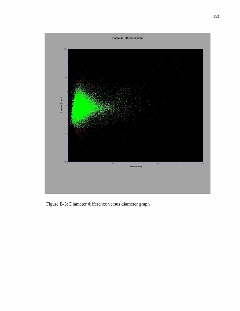
152

Figure B-3: Diameter difference versus diameter graph

153

Appendix C: Axial and Radial Variation of D30/D32 and D30/D-10

Ratios of the FFN

(a)

(b)

0.77

0.78

0.79

0.8

0.81

0.82

0.83

0.84

0.85

0 10 20 30 40

D30/D

32

z (mm)

Axial variation of D30/D32

at Ql=0.1 (µl/s)

Qg=215 (ml/min)

Qg=205 (ml/min)

Qg=194 (ml/min)

Qg=182 (ml/min)

Qg=169 (ml/min)

Qg=154 (ml/min)

0.75

0.76

0.77

0.78

0.79

0.8

0.81

0.82

0.83

0.84

0.85

0 10 20 30 40

D3

0/D

32

z (mm)

Axial variation of D30/D32

at Ql=0.2 (µl/s)

Qg=219 (ml/min)

Qg=206 (ml/min)

Qg=195 (ml/min)

Qg=182 (ml/min)

Qg=170 (ml/min)

Qg=155 (ml/min)

154

(c)

(d)

Figure C-1: D30/D32 variation with axial location at Ql (μl/s) (a) 0.1, (b) 0.2, (c) 0.4 and (d) 0.6

(r=0 mm).

0.75

0.76

0.77

0.78

0.79

0.8

0.81

0.82

0.83

0.84

0.85

0 10 20 30 40

D30/D

32

z (mm)

Axial variation of D30/D32

at Ql=0.4 (µl/s)

Qg=219(ml/min)

Qg=206 (ml/min)

Qg=195 (ml/min)

Qg=183 (ml/min)

Qg=169 (ml/min)

Qg=155 (ml/min)

0.74

0.75

0.76

0.77

0.78

0.79

0.8

0.81

0.82

0.83

0.84

0.85

0 10 20 30 40

D30/D

32

z (mm)

Axial variation of D30/D32

at Ql=0.6 (µl/s)

Qg=219 (ml/min)

Qg=206 (ml/min)

Qg=196 (ml/min)

Qg=182 (ml/min)

Qg=169 (ml/min)

Qg=155 (ml/min)

155

(a)

(b)

1.45

1.5

1.55

1.6

1.65

1.7

1.75

1.8

1.85

0 10 20 30 40

D30/D

-10

z (mm)

Axial variation of D30/D-10

at Ql=0.1 (µl/s) Qg=215 (ml/min)

Qg=205 (ml/min)

Qg=194 (ml/min)

Qg=182 (ml/min)

Qg=169 (ml/min)

Qg=154 (ml/min)

1.4

1.5

1.6

1.7

1.8

1.9

2

2.1

2.2

0 10 20 30 40

D30/D

-10

z (mm)

Axial variation of D30/D-10

at Ql=0.2 (µl/s) Qg=219 (ml/min)

Qg=206 (ml/min)

Qg=195 (ml/min)

Qg=182 (ml/min)

Qg=170 (ml/min)

Qg=155 (ml/min)

156

(c)

(d)

Figure C-2: D30/D-10 variation with axial location at Ql (μl/s) (a) 0.1, (b) 0.2, (c) 0.4 and (d) 0.6

(r=0 mm).

1.4

1.5

1.6

1.7

1.8

1.9

2

2.1

2.2

0 10 20 30 40

D30/D

-10

z (mm)

Axial variation of D30/D-10

at Ql=0.4 (µl/s) Qg=219 (ml/min)

Qg=206 (ml/min)

Qg=195 (ml/min)

Qg=183 (ml/min)

Qg=169 (ml/min)

Qg=155 (ml/min)

1.4

1.5

1.6

1.7

1.8

1.9

2

2.1

2.2

0 10 20 30 40

D30/D

-10

z (mm)

Axial variation of D30/D-10

at Ql=0.6 (µl/s) Qg=219 (ml/min)

Qg=206 (ml/min)

Qg=196 (ml/min)

Qg=182(ml/min)

Qg=169 (ml/min)

Qg=155 (ml/min)

157

(a)

(b)

1.18

1.2

1.22

1.24

1.26

1.28

1.3

1.32

1.34

0 0.2 0.4 0.6 0.8 1 1.2

D30/D

-10

r (mm)

Radial variation of D30/D-10

at Ql=0.1 (µl/s)

Qg=212 (ml/min)

Qg=202 (ml/min)

Qg=188 (ml/min)

Qg=177 (ml/min)

Qg=165 (ml/min)

Qg=150 (ml/min)

1.2

1.25

1.3

1.35

1.4

1.45

1.5

0 0.2 0.4 0.6 0.8 1 1.2

D3

0/D

-10

r (mm)

Radial variation of D30/D-10

at Ql=0.2 (µl/s)

Qg=215 (ml/min)

Qg=204 (ml/min)

Qg=191 (ml/min)

Qg=179 (ml/min)

Qg=166 (ml/min)

Qg=151 (ml/min)

158

(c)

(d)

Figure C-3: D30/D-10 variation with radial location at z=10 (mm) and Ql (μl/s) (a) 0.1, (b) 0.2, (c)

0.4 and (d) 0.6

1.15

1.2

1.25

1.3

1.35

1.4

1.45

0 0.2 0.4 0.6 0.8 1 1.2

D30/D

-10

r (mm)

Radial variation of D30/D-10

at Ql=0.4 (µl/s)

Qg=215 (ml/min)

Qg=204 (ml/min)

Qg=191 (ml/min)

Qg=180 (ml/min)

Qg=165 (ml/min)

Qg=151 (ml/min)

1.15

1.2

1.25

1.3

1.35

1.4

1.45

0 0.2 0.4 0.6 0.8 1 1.2

D30/D

-10

r (mm)

Radial variation of D30/D-10

at Ql=0.6 (µl/s)

Qg=216 (ml/min)

Qg=206 (ml/min)

Qg=192 (ml/min)

Qg=180 (ml/min)

Qg=167 (ml/min)

Qg=154 (ml/min)

159

(a)

(b)

0.76

0.77

0.78

0.79

0.8

0.81

0.82

0.83

0.84

0 0.2 0.4 0.6 0.8 1 1.2

D30/D

32

r (mm)

Radial variation of D30/D32

at Ql=0.1 (µl/s)

Qg=212 (ml/min)

Qg=202 (ml/min)

Qg=188 (ml/min)

Qg=177 (ml/min)

Qg=165 (ml/min)

Qg=150 (ml/min)

0.7

0.72

0.74

0.76

0.78

0.8

0.82

0 0.2 0.4 0.6 0.8 1 1.2

D3

0/D

32

r (mm)

Radial variation of D30/D32

at Ql=0.2 (µl/s)

Qg=215 (ml/min)

Qg=204 (ml/min)

Qg=191 (ml/min)

Qg=179 (ml/min)

Qg=166 (ml/min)

Qg=151 (ml/min)

160

(c)

(d)

Figure C-4: D30/D32 variation with radial location at z=10 (mm) and Ql (μl/s) (a) 0.1, (b) 0.2, (c)

0.4 and (d) 0.6.

0.67

0.69

0.71

0.73

0.75

0.77

0.79

0.81

0.83

0.85

0 0.2 0.4 0.6 0.8 1 1.2

D30/D

32

r (mm)

Radial variation of D30/D32

at Ql=0.4 (µl/s)

Qg=215 (ml/min)

Qg=204 (ml/min)

Qg=191 (ml/min)

Qg=180 (ml/min)

Qg=165 (ml/min)

Qg=151 (ml/min)

0.7

0.72

0.74

0.76

0.78

0.8

0.82

0.84

0.86

0 0.2 0.4 0.6 0.8 1 1.2

D30/D

32

r (mm)

Radial variation of D30/D32

at Ql=0.6 (µl/s)

Qg=216 (ml/min)

Qg=206 (ml/min)

Qg=192 (ml/min)

Qg=180 (ml/min)

Qg=167 (ml/min)

Qg=154 (ml/min)

161

Appendix D: Spatial Variation of Mean Droplet Velocity Moments

(a)

(b)

Figure D-1: Variation of (a) U10/ug and (b) Urms/U10 ratios with axial location for FFN at Ql=0.4

(µl/s) and different gas flow rates.

1

1.05

1.1

1.15

1.2

1.25

1.3

1.35

1.4

0 10 20 30 40

U10/u

g

z (mm)

Axial variation of U10/ug for FFN

Qg= 215 (ml/min)

Qg= 205 (ml/min)

Qg= 195 (ml/min)

Qg= 185 (ml/min)

Qg= 170 (ml/min)

Qg= 155 (ml/min)

0.3

0.35

0.4

0.45

0.5

0.55

0.6

0 10 20 30 40

Urm

s/U

10

z (mm)

Axial variation of Urms/U10 for FFN

Qg= 215 (ml/min)

Qg= 205 (ml/min)

Qg= 195 (ml/min)

Qg= 185 (ml/min)

Qg= 170 (ml/min)

Qg= 155 (ml/min)

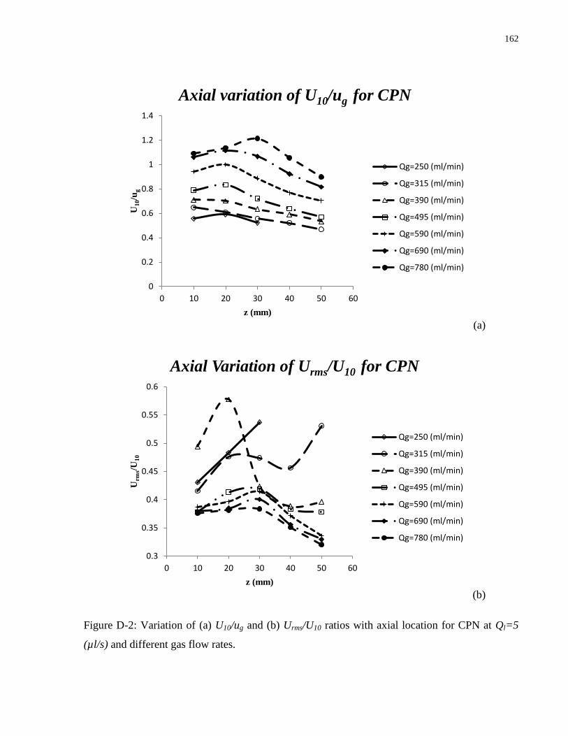
162

(a)

(b)

Figure D-2: Variation of (a) U10/ug and (b) Urms/U10 ratios with axial location for CPN at Ql=5

(µl/s) and different gas flow rates.

0

0.2

0.4

0.6

0.8

1

1.2

1.4

0 10 20 30 40 50 60

U10/u

g

z (mm)

Axial variation of U10/ug for CPN

Qg=250 (ml/min)

Qg=315 (ml/min)

Qg=390 (ml/min)

Qg=495 (ml/min)

Qg=590 (ml/min)

Qg=690 (ml/min)

Qg=780 (ml/min)

0.3

0.35

0.4

0.45

0.5

0.55

0.6

0 10 20 30 40 50 60

Urm

s/U

10

z (mm)

Axial Variation of Urms/U10 for CPN

Qg=250 (ml/min)

Qg=315 (ml/min)

Qg=390 (ml/min)

Qg=495 (ml/min)

Qg=590 (ml/min)

Qg=690 (ml/min)

Qg=780 (ml/min)

163

(a)

(b)

Figure D-3: Variation of (a) U10/ug and (b) Urms/U10 ratios with axial location for FFN at Ql=0.4

(µl/s) and different gas flow rates.

1

1.05

1.1

1.15

1.2

1.25

1.3

1.35

1.4

0 10 20 30 40

U10/u

g

z (mm)

Axial variation of U10/ug for FFN

Qg= 215 (ml/min)

Qg= 205 (ml/min)

Qg= 195 (ml/min)

Qg= 185 (ml/min)

Qg= 170 (ml/min)

Qg= 155 (ml/min)

0.3

0.35

0.4

0.45

0.5

0.55

0.6

0 10 20 30 40

Urm

s/U

10

z (mm)

Axial variation of Urms/U10 for FFN

Qg= 215 (ml/min)

Qg= 205 (ml/min)

Qg= 195 (ml/min)

Qg= 185 (ml/min)

Qg= 170 (ml/min)

Qg= 155 (ml/min)

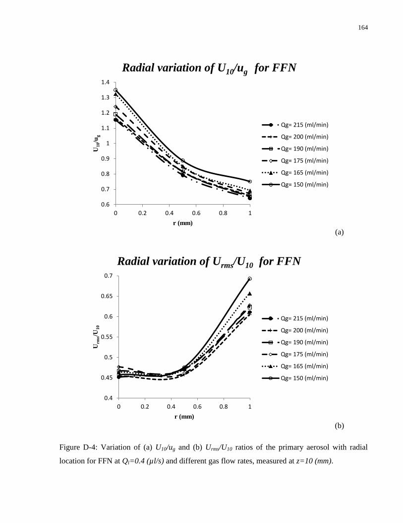
164

(a)

(b)

Figure D-4: Variation of (a) U10/ug and (b) Urms/U10 ratios of the primary aerosol with radial

location for FFN at Ql=0.4 (µl/s) and different gas flow rates, measured at z=10 (mm).

0.6

0.7

0.8

0.9

1

1.1

1.2

1.3

1.4

0 0.2 0.4 0.6 0.8 1

U10/u

g

r (mm)

Radial variation of U10/ug for FFN

Qg= 215 (ml/min)

Qg= 200 (ml/min)

Qg= 190 (ml/min)

Qg= 175 (ml/min)

Qg= 165 (ml/min)

Qg= 150 (ml/min)

0.4

0.45

0.5

0.55

0.6

0.65

0.7

0 0.2 0.4 0.6 0.8 1

Urm

s/U

10

r (mm)

Radial variation of Urms/U10 for FFN

Qg= 215 (ml/min)

Qg= 200 (ml/min)

Qg= 190 (ml/min)

Qg= 175 (ml/min)

Qg= 165 (ml/min)

Qg= 150 (ml/min)

165

Appendix E: Empirical Probability Distribution Functions

The classical method of modeling drop size distributions is empirical (93): a curve is fit to data

collected for a wide range of atomizer nozzles and operating conditions. Curves appearing

frequently become the basis for standard empirical distributions. Some of the most commonly

used distributions are listed below.

Gauss-Normal distribution:

The normal distribution is a number-based continuous bell shaped function and perhaps the

simplest form of distribution functions. The function is defined by having a mean (D10) and a

variance (ν=Drms/D10) parameter with a peak located at the mean. The skewness of the function

is zero that implies the function is essentially symmetric with respect to the mean value.

( ) √

{

( )

} (E-1)

Log-Normal distribution:

If a variate x is distributed so that the distribution of the transformed variate y=ln(x) is Gaussian,

then the variate x is said to be log normally distributed. Therefore:

( )

( )√ {

( )

( )} (E-2)

Where D’ represents the logarithmic mean of size distribution and ζLN represent the width of the

distribution. It is interesting to note that the log-normal distribution is arises when one considers

the theoretical distribution that is produced by continuous random partitioning of a set of sand

particles that was first noticed by Kolmogoroff (96).

Upper-limit distribution:

This distribution is a modification of the log-normal distribution in that a maximum drop size is

introduced:

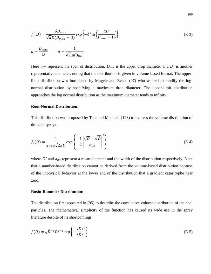
166

( )

√ ( ) { (

)} (E-3)

√ ( )

Here ζUL represent the span of distribution, Dmax is the upper drop diameter and D’ is another

representative diameter, noting that the distribution is given in volume-based format. The upper-

limit distribution was introduced by Mugele and Evans (97) who wanted to modify the log-

normal distribution by specifying a maximum drop diameter. The upper-limit distribution

approaches the log normal distribution as the maximum diameter tends to infinity.

Root-Normal Distribution:

This distribution was proposed by Tate and Marshall (128) to express the volume distribution of

drops in sprays.

( )

√ {

[√ √

]

} (E-4)

where D’ and ζRN represent a mean diameter and the width of the distribution respectively. Note

that a number-based distribution cannot be derived from the volume-based distribution because

of the unphysical behavior at the lower end of the distribution that a gradient catastrophe near

zero.

Rosin-Rammler Distribution:

The distribution first appeared in (95) to describe the cumulative volume distribution of the coal

particles. The mathematical simplicity of the function has caused its wide use in the spray

literature despite of its shortcomings.

( ) { (

)

} (E-5)

167

here D’ and q are the mean and with of the distribution. Small values of q are associated with

broad sprays and large values result in narrow sprays. For many droplet generation processes, q

ranges from 1.5 to 4, and for rotary atomization q might be as large as 7 whereas monodisprse

spray production demands a q value of infinity (94).

Nukiyama-Tanasawa Distribution:

The distribution is proposed by Nukiyama and Tanasawa (51) to describe the number-based

distribution of sprays from pneumatic nebulizers and resembles the Rosin-Rammler distribution

mathematically.

( ) ( ) (E-6)

where b, p and q are adjustable parameters that control the location of mean and span of the

distribution. a is a normalizing constant and p is sometimes taken to be two. According to

Paloposki (129), physical meaningful results are produced either if p>1 and q>0 or p<-4 and

q<0.

Log-Hyperbolic Distribution:

This function is first applied to sprays by Bhatia et al. (98), (124) and (125) which has the given

form:

( ) ( ) { √ ( ) ( )} (E-7)

here a is a normalizing constant

√

( √ ) (E-8)

and K1 is the modified Bessel function of the first kind and first order. The constraints on the

parameters are as follows: -∞<D<∞, α>0, |β|< α, δ>0 and -∞<µ<∞. The distribution derives its

name from the fact that the logarithm of the probability distribution function is a hyperbola. δ is

the scale parameter, µ is the location parameter and the remaining two parameters describe the

shape of the pdf.

168

The distribution is one of the most successful empirical distributions as it can be fit to a wide

range of experimental data. But it requires extensive and tedious mathematical calculations (93)

and the parameters of the distribution are mathematically unstable (115) which is highly

undesirable.

169

Appendix F: Derivation of Shannon entropy

Consider a size and velocity space shown in Figure 5-1. If the total number of droplets is given

by Ntot, then the number of possible ways to put ΔN1,1 droplets in the first class of size and

velocity will be:

(

)

( ) (F-1)

Once, the ΔN1,1 droplets are placed in the first classes of size and velocity, we can similarly find

the number of ways that ΔN1,2 (out of Ntot-ΔN1,1 droplets) can be placed in the second class of

velocity and first class of size.

(

)

( )

( ) (F-2)

This procedure can be continued until all the droplets are distributed in size and velocity space.

Then the total number of possible states can be written by:

(

) (

) (

∑ ∑

) (F-3)

∑

Equation (F-3) can be simplified by using Equations (F-1) and (F-2) to:

(F-4)

We are now seeking an entropy function as a measure of disorder of the system based on the

total number of possible states given by W. Chakrabarti (130) have proven on the basis of two

fundamental properties of thermodynamic entropy, the form of entropy function can be derived,

which are:

170

(i) The entropy S(W) of system is a positive increasing function of the disorder W, that

is:

( ) ( ) (F-5)

(ii) The entropy S(W) is assumed to be an additive function of the disorder W, that is, for

any two statistically independent systems with degreed of disorder W1 and W2

respectively, the entropy of the composite system is given by:

( ) ( ) ( ) (F-6)

Proof:

Let’s assume that W>e. This is justified by the fact that the macroscopic system we are

interested in consist of large number of microstates and hence corresponds to a large value of

statistical weight W. For any integer n, we can find an integer m(n) such that:

( ) ( ) (F-7)

or

( )

( )

( )

(F-8)

Consequently:

( )

( ) (F-9)

The entropy function S(W) must satisfy both (i) and (ii) conditions. From the first condition it

draws:

( ( )) ( ) ( ( ) ) (F-10)

again from (ii) and (C-10) we have:

( ) ( ) ( ) ( ( ) ) ( ) (F-11)

171

and as a result:

( )

( )

( ) (F-12)

By comparing (F-9) and (F-12), we get:

( ) ( ) (F-13)

Where S(e)=k is a positive constant that depends on the unit of measurement of entropy. The

positivity follows from the positivity of the entropy function postulated from (i).

Now that the form of entropy function is determined, we may further expand Equation (F-13) by

having the statistical weigh function W given in (F-4):

( ) ( ) { ( ) (∑∑ )} (F-14)

Equation (F-14) can be simplified by Sterling’s approximation ln (x!)=x ln (x) –x to:

( ) { ( ) ∑∑ ( ) ∑∑ } (F-15)

∑∑ (F-16)

Therefore:

( ) ∑∑(

) (

) ∑∑ ( ) (F-17)

and the entropy per unit number of droplet would be:

( ) ( )

∑∑ ( ) (F-18)

172

Appendix G: Bayesian and Shannon entropy

In probability theory and information theory, the Kullback–Leibler divergence (also information

divergence, information gain, or relative entropy) is a measure of the difference between two

probability distributions: from a "true" probability distribution P to an arbitrary probability

distribution Q.

Typically P represents data, observations, or a precise calculated probability distribution. The

measure Q typically represents a theory, a model, a description or an approximation of P.

For distributions P and Q of a continuous random variable the K–L divergence of Q from P is

defined to be:

( ) ∫ ( ) ( ( )

( ))

(G-1)

Equation (1-D) is equivalent to the measure of nearness of two probability density functions.

Minimizing the K-L equation subjected to a set of constraints is also identical to maximizing

Bayesian entropy, which is a measure that takes a priori distributions into account.

Shannon entropy is in fact a special case of the Bayesian entropy when the priori distribution is

uniform one, that is Q(x) =1. In other words, maximizing the Shannon entropy with only the

normalization constraint would result in a uniform distribution but in the absence of any other

constraints, maximization of Bayesian entropy gives distribution Q(x).

173

Nomenclature

Ac Cross sectional area of droplet

CD Drag coefficient

do Orifice diameter

dj Jet diameter

D Droplet diameter

D-10 Nameless characteristic mean size diameter

D30 Mass mean diameter

D32 Sauter mean diameter

Dcap Capillary diameter

Dp Prefilmer lip diameter, pipe diameter

Dref Reference velocity

f Joint size and velocity probability distribution function

fb Breakup frequency

ho Total gas enthalpy

H Distance between capillary and orifice plate in FFN

J Jacobian Matrix

k Specific heat ratio, Constant of entropy

K Constant of axial velocity profile

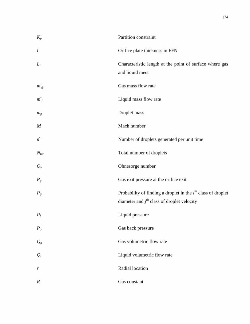
174

Kp Partition constraint

L Orifice plate thickness in FFN

Lc Characteristic length at the point of surface where gas

and liquid meet

m•g Gas mass flow rate

m•l Liquid mass flow rate

mp Droplet mass

M Mach number

n• Number of droplets generated per unit time

Ntot Total number of droplets

Oh Ohnesorge number

Pg Gas exit pressure at the orifice exit

Pij Probability of finding a droplet in the ith

class of droplet

diameter and jth

class of droplet velocity

Pl Liquid pressure

Po Gas back pressure

Qg Gas volumetric flow rate

Ql Liquid volumetric flow rate

r Radial location

R Gas constant

175

Re Reynolds number

s Shannon entropy

Tg Gas exit temperature at the orifice exit

To Gas back temperature

ug Gas exit velocity at the orifice

uj Liquid jet velocity

ul Liquid exit velocity at the orifice

u* Sonic velocity

U Droplet velocity

U10 Droplet mean velocity

Ucap Liquid capillary velocity

UR Relative velocity between liquid and gas the orifice exit

Uref Reference velocity

Urms Droplet root mean square velocity

up Particle velocity

w Constraint number

We Weber number

z Axial location

176

Greek Symbols

γ Characteristic moment

εT Turbulent kinematic viscosity

η Atomization efficiency

ηl Liquid viscosity

λ Wavelength

ρg Gas exit density at the orifice exit

ρl Liquid density

ρo Gas back density

σ Surface tension

η*

Sheet thickness at point of breakup

ηs

Tangential viscous stress on the jet surface

υ Kinematic viscosity