africa supraregional - startseite
TRANSCRIPT

Africa SupraregionalAdaptation to Climate Change in the Lake Chad Basin
CLIMATE CHANGE STUDY
Africa SupraregionalAdaptation to Climate Change in the Lake Chad Basin
CLIMATE CHANGE STUDY
Africa Supraregional – Adaptation to Climate Change in the Lake Chad Basin2 3Table of Contents
List of TablesTable 1: Geological time table 13Table 2: Some typical crops under rainfed conditions (FAO, 2004) 19
List of FiguresFigure 1: General paths of the Sahabi and Eosahabi Rivers together with possible paths of the
Palaeosahabi Rivers (after GRIFFIN, 2006) 14Figure 2: Schematic presentation of the seasonal migration of the ITCZ 15Figure 3: Observed mean precipitation from RFE data (left) and down-scaled precipitation (right) in LCB 18Figure 4: Long-term annual means for annual cycles of temperature, precipitation and PET ,
calculated for different climate zones in the Lake Chad Basin. 19Figure 5: Aridity zones in LCB calculated as the quotient of ‘Annual Precipitation/Annual PET’ 20Figure 6: Two cycles showing the aridity index at 10-day intervals 20Figure 7: Classification of vegetation phenologies and reference vegetation cycles 21Figure 8: Frequency of bush fires between 2001 and 2013 22Figure 9: Annual precipitation anomalies 23Figure 10: Grid displaying CRUTEM4 pixel size and location 23Figure 11: Changes in annual temperature (CRUTEM4 data) in the LCB 24Figure 12: Seasonal temperature trends 25Figure 13: Temperature change between 2000 and 2099 28Figure 14: Seasonal temperature change under a B1 scenario 29Figure 15: Seasonal temperature change under an A1b scenario 30Figure 16: Seasonal temperature change under an A2 scenario 31Figure 17: Annual total precipitation in the arid (top) and semi-arid (bottom) zone 33Figure 18: Average position of the 120-day line (green) between 2001 and 2013. 34Figure 19: Retreat of the 120-day line under a B1 (yellow) and an A2 (red) scenario 35Figure 20: Shift of vegetation (ecological) boundaries - B1 scenario 36Figure 21: Shift of vegetation (ecological) boundaries - A2 scenario 37Figure 22: Geomorphological setting of the Yaere-Naga wetlands 39Figure 23: River discharge at Bongor, Katoa and Logone-gana stations 40Figure 24: Discharge thresholds for Logone water losses 40Figure 25: Correlation between rainfall in the Bongor catchment and river discharge measured at Bongor 41Figure 26: Total water losses in the effective run-off area of the Logone River 41Figure 27: Classification of vegetation cycles (phenology) 42Figure 28: Spatial distribution of human activities 43Figure 29: Annual total river discharge at station N’djamena 44Figure 30: Additional evaporation from open water surfaces assuming a current lake extent
and a 1963 lake surface 44Figure 31: Settlements in and around Lake Chad. 45Figure 32: Absolute seasonal temperature change between 2000-2009 - B1 scenario 47Figure 33: Absolute seasonal temperature change between 2000-2009 and 2040-2049 - A2 scenario 48Figure 34: Absolute seasonal temperature change between 2000-2009 and 2070-2079 - B1 scenario 49Figure 35: Absolute seasonal temperature change between 2000-2009 and 2070-2079 - A2 scenario 50Figure 36: Absolute seasonal temperature change between 2000-2009 and 2090-2099 - B1 scenario. 51Figure 37: Absolute seasonal temperature change between 2000-2009 and 2090-2099 - A2 scenario 52Figure 38: Original temperatures (left) and downscaled temperatures (right) 53Figure 39: Original precipitation data (left) and downscaled precipitation (right) 53Figure 40: Look-up function for converting PETHARGREAVES into PETPENMAN. 54Figure 41: Comparison between modeled and observed soil moisture at different depths. 55Figure 42: Fourier filtered biomass cycle (red curve; created through inverse Fourier transform) after
removing noise (blue curve) from the original biomass cycle (green curve) using a discrete Fourier transform function. 57
Figure 43: Magnitudes (left) and phases (right) of a biomass cycle as shown in Figure 42. 57Figure 44: Average number of days an area exceeds dry sub-humid conditions in 2010-2019 58
Table of Contents1 Executive Summary 7
2 Introduction 11
3 Climate in the Lake Chad Basin 133.1 Messinian (Neogene) Lake Chad 133.2 Lake Mega Chad 14
4 Current and Past Climate Variations / Changes 174.1 Current Climate Situation in the Lake Chad Basin 174.2 Past Climate Variation and Change 224.2.1 Long-term precipitation development 1901 – 2010 224.2.2 Long-term temperature development between 1953/73 and 2013 23
5 Future Climate Change 275.1 General Circulation Models (GCM) 275.2 Climate Change Scenarios 275.3 Data Preparation 285.4 Climate Change under Different Scenarios 285.4.1 Temperature 285.4.2 Precipitation 325.5 Impact of Climate Change on the Length of the Growing Period 33
6 Yaere – Naga Wetlands 396.1 Lake Chad 43
7 Annex 477.1 Seasonal Temperature Change 477.2 Spatial Downscaling of GCM Data 537.3 Spatial Downscaling, Temperatures 537.4 Spatial Downscaling, Precipitation 537.5 Hydrologic Modelling 547.5.1 Potential Evapotranspiration 547.5.2 Equations used in hydrologic modelling 557.6 Classification of Vegetation Cycles (Ecosystems) 567.7 Length of Growing Period 587.8 PET Increase 637.9 Impacts of Rainfall Characteristics on Surface Run-off 68
8 References 69
Africa Supraregional – Adaptation to Climate Change in the Lake Chad Basin4 5
Figure 45: Average number of days an area exceeds dry sub-humid conditions in 2020-2029 59Figure 46: Average number of days an area exceeds dry sub-humid conditions in 2030-2039 59Figure 47: Average number of days an area exceeds dry sub-humid conditions in 2040-2049 60Figure 48: Average number of days an area exceeds dry sub-humid conditions in 2050-2059 60Figure 49: Average number of days an area exceeds dry sub-humid conditions in 2060-2069 61Figure 50: Average number of days an area exceeds dry sub-humid conditions in 2070-2079 61Figure 51: Average number of days an area exceeds dry sub-humid conditions in 2080-2089 62Figure 52: Average number of days an area exceeds dry sub-humid conditions in 2090-2099 62Figure 53: PET Increase by 2010-2019 for a B1 (left) and an A2 Scenario (right) 63Figure 54: PET Increase by 2020-2029 for a B1 (left) and an A2 Scenario (right) 63Figure 55: PET Increase by 2030-2039 for a B1 (left) and an A2 Scenario (right) 64Figure 56: PET Increase by 2040-2049 for a B1 (left) and an A2 Scenario (right) 64Figure 57: PET Increase by 2050-2059 for a B1 (left) and an A2 Scenario (right) 65Figure 58: PET Increase by 2060-2069 for a B1 (left) and an A2 Scenario (right) 65Figure 59: PET Increase by 2070-2079 for a B1 (left) and an A2 Scenario (right) 66Figure 60: PET Increase by 2080-2089 for a B1 (left) and an A2 Scenario (right) 66Figure 61: PET Increase by 2090-2099 for a B1 (left) and an A2 Scenario (right) 67Figure 62: Comparison of observed and modelled run-off 68
List of Acronyms
List of AcronymsAHT AHT GROUP AG, Management & Engineering, Essen/GermanyAI Aridity IndexBGR Bundesanstalt für Geowissenschaften und Rohstoffe (Federal Institute for Geosciences and
Natural Resources), Hannover/GermanyCC Climate ChangeCCCSN Canadian Climate Change Scenarios NetworkCCSM Community Climate System ModelCGSM Canadian General Circulation ModelCRUTEM Climate Research Unit Temperature (Hadley Climate Centre, GB)DFT Discrete Fourier TransformDOY Day of YearDSMW Digital Soil Map of the World (FAO)DWD Deutscher WetterdienstFAO Food and Agricultural Organisation of the United NationsGCM General Circulation ModelGIZ GmbH Gesellschaft für Internationale Zusammenarbeit GmbH, Eschborn/GermanyGMTED 2010 Global Multi-resolution Terrain Elevation Data 2010GPCC Global Precipitation Climate Center (of the DWD)HadGEM Hadley Centre Global Environment ModelHWSD Harmonized World Soil Database (FAO)IPCC Intergovernmental Panel on Climate ChangeITCZ Intertropical Convergence ZoneLCB Lake Chad BasinLCBC Lake Chad Basin CommissionNCDC National Climate Data CentreNDVI Normalized Difference Vegetation IndexPET Potential Evapo-TranspirationRFE Rainfall EstimatesSST Sea Surface TemperatureTOA Top of Atmosphere RadiationUNEP United Nations Environment Program

Africa Supraregional – Adaptation to Climate Change in the Lake Chad Basin6
Climate change therefore has an acute impact on ag-riculture, cattle farming and fisheries. The high level of rainfall variability poses a risk to production on land that is traditionally farmed through rainfed agricul-ture, irrigation and flood recession farming, as well as from pastureland and fishing. A lack of rainfall leads to failed harvests and damages natural vegetation. Heavy rainfall causes flooding and erodes farmland. These changes in climate conditions result in increased food insecurity, social tensions and poverty, and cause a rise in the number of refugees among the affected population.
To address these challenges, the German cooperation project “Adaptation to Climate Change in the Lake Chad Basin’ (ACC) was initiated. The project is part of the programme “Sustainable Water Management Lake Chad Basin” of the German Federal Ministry for Economic Cooperation and Development (BMZ) and the Lake Chad Basin Commission, implemented by the Deutsche Gesellschaft für Internationale Zusam-menarbeit (GIZ) GmbH. Basis for this project is the Climate Change Study, executed by the AHT GROUP AG, with several modelling, addressing various as-sumptions in climate change. This allows the assess-ment of possible future climate trends, possible im-pacts on ecosystems within the Lake Chad Basin and socio-economic consequences. The climate change study provides the knowledge base as input and con-tribution for the LCBC Climate Change Adaptation Strategy Development.
Climate change under various change scenarios is mostly driven by a temperature increase. Precipitation slightly increased until mid-20th century, however
According to the Intergovernmental Panel on Climate Change (IPCC), climate change and the resulting increase in temperatures and rainfall variability are set to have a particularly serious impact on agriculture in the Sahel zone. Droughts and flooding have in-creased considerably in the Sahel region since the 1970s. According to the United Nations Environment Programme (UNEP), half of the shrinkage of Lake Chad can be ascribed to the impact of climate change and climate variability. The other half is the result of the in-creased demand for water from Lake Chad’s tributaries for irrigation and the needs of growing populations, particularly in Nigeria, Cameroon and Chad.
The Lake Chad Basin is one of the largest sedimentary closed groundwater basins in the whole of Africa. With its extensive pasture and arable land and rich fish stocks, it is an important area both economically and environmentally for the riparian states of Chad, Nigeria, the Niger, Cameroon, the Central African Re-public and Libya. Lake Chad and its tributaries form an important water reservoir in the central Sahel region. Founded in 1964 by the lake’s riparian states, the Lake Chad Basin Commission (LCBC) is mandated to conserve natural resources, monitor and coordinate cross-border water projects, regulate and control water use and resolve disputes. Its mandate also includes advising member states on dealing with the effects of climate change, particularly with regard to agricultural development (food security).
Around 38 million people from diverse ethnic back-grounds currently live in the Lake Chad Basin. Most of these people are from poor rural households and survive on subsistence farming.
Executive Summary17
Africa Supraregional – Adaptation to Climate Change in the Lake Chad Basin8 9Notes
Basin. Shifts are smallest towards the eastern (upper Komadugu-Yobe basin) and western basin periphery (area south of Am Timan). Total area losses amount to 70,960 km2 (B1 scenario) and 135,150 km2 (A2 scenario) until the end of the century. Because of large displacements in the central basin (east of Bongor), these areas could well be targeted for introducing al-ternative cropping practices. Parts of this area fall into the intervention zone of the GIZ program module.
The future situation of wetland areas that do not fall under the 120-day line rule, because these areas receive additional water from river discharge, is more difficult to predict. Upstream surface run-off, a major source of water for downstream wetlands, cannot be modeled reliably from monthly GCM data. A compar-ison of the wetland situation during a dry and a wet year suggests a general shrinking of e.g. the Yaere-Naga wetlands with some fragmentation of wetted areas. Human activities seem to have adjusted already to this situation and are concentrated on the wetland core that receives substantial wetting even during dry years. Due to increased evapotranspiration rates, the duration of the growing period of wetland vegetation will likely be shorter, but without falling below typical cropping periods.
Evaporation from open water surfaces such as Lake Chad will increase by about 5 % (B1) to 11 % (A2). Assuming a continuous discharge into the lake at the current level will certainly allow preserving Lake Chad within its current shorelines and some spillovers into the northern pond to sustain agricultural activities.
Where such water resources (northern pond) are not available, agricultural activities should focus on the basin’s hinterland, where evaporation rates are lower.
started decreasing thereafter, reaching a minimum during the droughts of the 70ies and 80ies. No significant difference in temperature development is forecasted until the 2040ies. After 2049, temperatures under an A2 scenario will rise more quickly while B1 temperatures gradually taper off.
The modeling results forecast the highest projected increase of mean annual temperature for the central and the eastern Lake Chad Basin reaching in some areas up to 3 °C (B1) or almost 6 °C (A2) by the end of this century. Increases will be highest during spring and fall.
Rising temperatures will increase evaporation/evapo-transpiration, thus reducing the available water resources by up to 4 % (B1) and nearly 10 % (A2) until 2099. While at the beginning of this century, clear dif-ferences exist in reduced availability of water depend-ing on climatic region, reductions will be almost equal to all climate zones by the end of the 21st century. Projected climate change will be the cause for a gradual southward shift of ecosystems within the Lake Chad Basin. Displacements will be smallest in dry areas (north) and increase to the south causing larger shifts and fragmentation in ecosystems of the more humid climates. A crucial transition is the line marking the 120-day growing period. It roughly sep-arates the more intensely cultivated areas from areas with only scattered farming activities. According to FAO, this line is a threshold between drought resistant breeds of a short vegetative period and more valuable and water demanding crops. The line is calculated from precipitation and potential evapotranspiration and ignores the special situation of wetland areas.
Over the 21st century the east-west stretching line will gradually shift south with largest losses of cropping areas occurring in the central part of the Lake Chad

Africa Supraregional – Adaptation to Climate Change in the Lake Chad Basin10 11
perature. Other parameters affecting agricultural potentials are various soil parameters, topography and sometimes groundwater. These parameters are considered as temporally stable, and are therefore not included in the analyses. Significant agricultural changes however may be experienced due to changes in the run-off situation. In areas where agriculture not only depends on local rainfall but also on stream water (irrigated agriculture, wetland areas), changes in total discharge and in peak flow (affecting inundation) may lead to a deterioration of agricultural potentials. The situation of drainage systems is addressed in this study as far as data are available.
Different hydro-meteorological (e.g. potential evapo-transpiration) or climatic parameters (e.g. aridity index) are calculated for improved comprehension of the combined impact of rainfall and temperature on vegetation. Other variables used include outputs from hydrologic modeling i.e. soil moisture and surface run-off.
Climate parameters describing future climate change scenarios are taken from GCMs. While GCMs are rather accurate in forecasting global climate variation and change these are significantly less detailed in the prediction of local climate change. In parts, this is a matter of the coarse resolution of GCMs smoothing or neglecting physical processes at a local scale. To lessen the influence of a coarse spatial resolution, several sta-tistical improvements (downscaling) are applied.Chapter 7 describes the details on the models and algorithms applied in this study. All figures included in this report except for Figure 2 are prepared using the calculation and modelling results as described within the respective chapters.
This study analyzes possible impacts of projected future climate change on ecosystems of the Lake Chad Basin. Results are intended to serve as an orientation to realize the severity of changes and their spatial distribution and serve as a basis for developing adaptation strategies. For the agricultural areas, it is of particular interest to understand how the agricultural potentials may change under various climate change scenarios. Further, this study will provide the knowl-edge base (as input and contribution) for the LCBC Climate Change Adaptation Strategy Development.
In a first step, the study (i) calculates the impact on the boundaries of the Sahel for different time horizons and (ii) assesses the impact on monthly flood volumes of Logone and Chari rivers. In step 2 the study assesses the impact of changing discharge patterns on agricul-tural production models, considering (i) change in precipitation, (ii) availability of floodwater from the spillover of the two principal rivers, and (iii) last not least increased evapotranspiration.
Due to size of the Lake Chad Basin, a detailed mapping/analysis of e.g. individual agricultural areas and their situation under different climate conditions is not feasible. The reliable distinction of agricultural areas in Central Africa is particularly complex due to the spec-tral and textural appearance, the seasonal cycles and the similarity of these features with natural vegetation cover. A reliable distinction requires the analysis of a considerable number of high-resolution satellite data, a time-consuming process that was impossible to accom-plish within the allotted time for this study.
This study focuses on the analysis of agricultural potentials primarily controlled by rainfall and tem-
Introduction2
Africa Supraregional – Adaptation to Climate Change in the Lake Chad Basin12 13
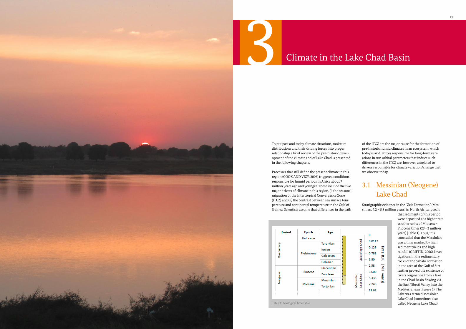
of the ITCZ are the major cause for the formation of pre-historic humid climates in an ecosystem, which today is arid. Forces responsible for long-term vari-ations in sun orbital parameters that induce such differences in the ITCZ are, however unrelated to drivers responsible for climate variation/change that we observe today.
3.1 Messinian (Neogene) Lake Chad
Stratigraphic evidence in the “Zeit Formation” (Mes-sinian, 7.2 – 5.3 million years) in North Africa reveals
that sediments of this period were deposited at a higher rate as other units of Miocene - Pliocene times (23 - 2 million years) (Table 1). Thus, it is concluded that the Messinian was a time marked by high sediment yields and high rainfall (GRIFFIN, 2006). Inves-tigations in the sedimentary rocks of the Sahabi Formation in the area of the Gulf of Sirt further proved the existence of rivers originating from a lake in the Chad Basin flowing via the East Tibesti Valley into the Mediterranean (Figure 1). The Lake was termed Messinian Lake Chad (sometimes also called Neogene Lake Chad).
To put past and today climate situations, moisture distributions and their driving forces into proper relationship a brief review of the pre-historic devel-opment of the climate and of Lake Chad is presented in the following chapters.
Processes that still define the present climate in this region (COOK AND VIZY, 2006) triggered conditions responsible for humid periods in Africa about 7 million years ago and younger. These include the two major drivers of climate in this region, (i) the seasonal migration of the Intertropical Convergence Zone (ITCZ) and (ii) the contrast between sea surface tem-perature and continental temperature in the Gulf of Guinea. Scientists assume that differences in the path
Climate in the Lake Chad Basin3
Table 1: Geological time table
Africa Supraregional – Adaptation to Climate Change in the Lake Chad Basin14 15Climate in the Lake Chad Basin
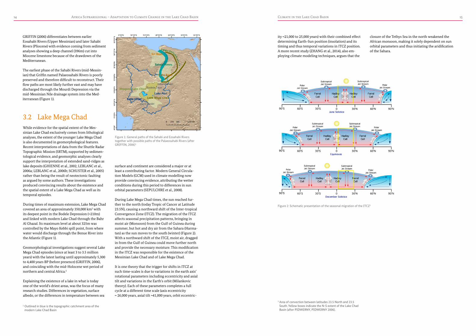
closure of the Tethys Sea in the north weakened the African monsoon, making it solely dependent on sun orbital parameters and thus initiating the aridification of the Sahara.
ity ~21,000 to 25,000 years) with their combined effect determining Earth-Sun position (insolation) and its timing and thus temporal variations in ITCZ position. A more recent study (ZHANG et al., 2014), also em-ploying climate modeling techniques, argues that the
GRIFFIN (2006) differentiates between earlier Eosahabi Rivers (Upper Messinian) and later Sahabi Rivers (Pliocene) with evidence coming from sediment analyses showing a deep channel (396m) cut into Miocene limestone because of the drawdown of the Mediterranean.
The earliest phase of the Sahabi Rivers (mid-Messin-ian) that Griffin named Palaeosahabi Rivers is poorly preserved and therefore difficult to reconstruct. Their flow paths are most likely further east and may have discharged through the Mourdi Depression via the mid-Messinian Nile drainage system into the Med-iterranean (Figure 1).
surface and continent are considered a major or at least a contributing factor. Modern General Circula-tion Models (GCM) used in climate modelling now provide convincing evidence, attributing the wetter conditions during this period to differences in sun orbital parameters (SEPULCHRE et al., 2008).
During Lake Mega Chad times, the sun reached fur-ther to the north (today Tropic of Cancer at Latitude 23.5N), causing a northward shift of the Inter-tropical Convergence Zone (ITCZ). The migration of the ITCZ affects seasonal precipitation patterns, bringing in moist air (Monsoon) from the Gulf of Guinea during summer, but hot and dry air from the Sahara (Harma-tan) as the sun moves to the south (winter) (Figure 2). With a northward shift of the ITCZ, moist air, dragged in from the Gulf of Guinea could move further north and provide the necessary moisture. This modification in the ITCZ was responsible for the existence of the Messinian Lake Chad and of Lake Mega Chad.
It is one theory that the trigger for shifts in ITCZ at such time-scales is due to variations in the earth axis’ rotational parameters including eccentricity and axial tilt and variations in the Earth’s orbit (Milankovic theory). Each of these parameters completes a full cycle at a different time scale (axis eccentricity ~ 26,000 years, axial tilt ~41,000 years, orbit eccentric-
3.2 Lake Mega ChadWhile evidence for the spatial extent of the Mes-sinian Lake Chad exclusively comes from lithological analyses, the extent of the younger Lake Mega Chad is also documented in geomorphological features. Recent interpretations of data from the Shuttle Radar Topographic Mission (SRTM), supported by sedimen-tological evidence, and geomorphic analyses clearly support the interpretation of extended sand-ridges as lake deposits (GHIENNE et al., 2002; LEBLANC et al., 2006a; LEBLANC et al., 2006b; SCHUSTER et al., 2005) rather than being the result of neotectonic faulting as argued by some authors. These investigations produced convincing results about the existence and the spatial extent of a Lake Mega Chad as well as its temporal episodes.
During times of maximum extension, Lake Mega Chad covered an area of approximately 350,000 km2 with its deepest point in the Bodele Depression (~210m) and linked with modern Lake Chad through the Bahr Al Ghazal. Its maximum level at about 325m was controlled by the Mayo Kebbi spill point, from where water would discharge through the Benue River into the Atlantic (Figure 1).
Geomorphological investigations suggest several Lake Mega Chad episodes (since at least 3 to 3.5 million years) with the latest lasting until approximately 5,300 to 4,400 years BP (before presence) (GRIFFIN, 2006), and coinciding with the mid-Holocene wet period of northern and central Africa.2
Explaining the existence of a lake in what is today one of the world’s driest areas, was the focus of many research studies. Differences in vegetation, surface albedo, or the differences in temperature between sea
Figure 2: Schematic presentation of the seasonal migration of the ITCZ3
Figure 1: General paths of the Sahabi and Eosahabi Rivers together with possible paths of the Palaeosahabi Rivers (after GRIFFIN, 2006)1
1 Outlined in blue is the topographic catchment area of the modern Lake Chad Basin
3 Area of convection between latitudes 23.5 North and 23.5 South. Yellow boxes indicate the N-S extent of the Lake Chad Basin (after PIDWERNY, PIDWERNY 2006).
Africa Supraregional – Adaptation to Climate Change in the Lake Chad Basin16 17
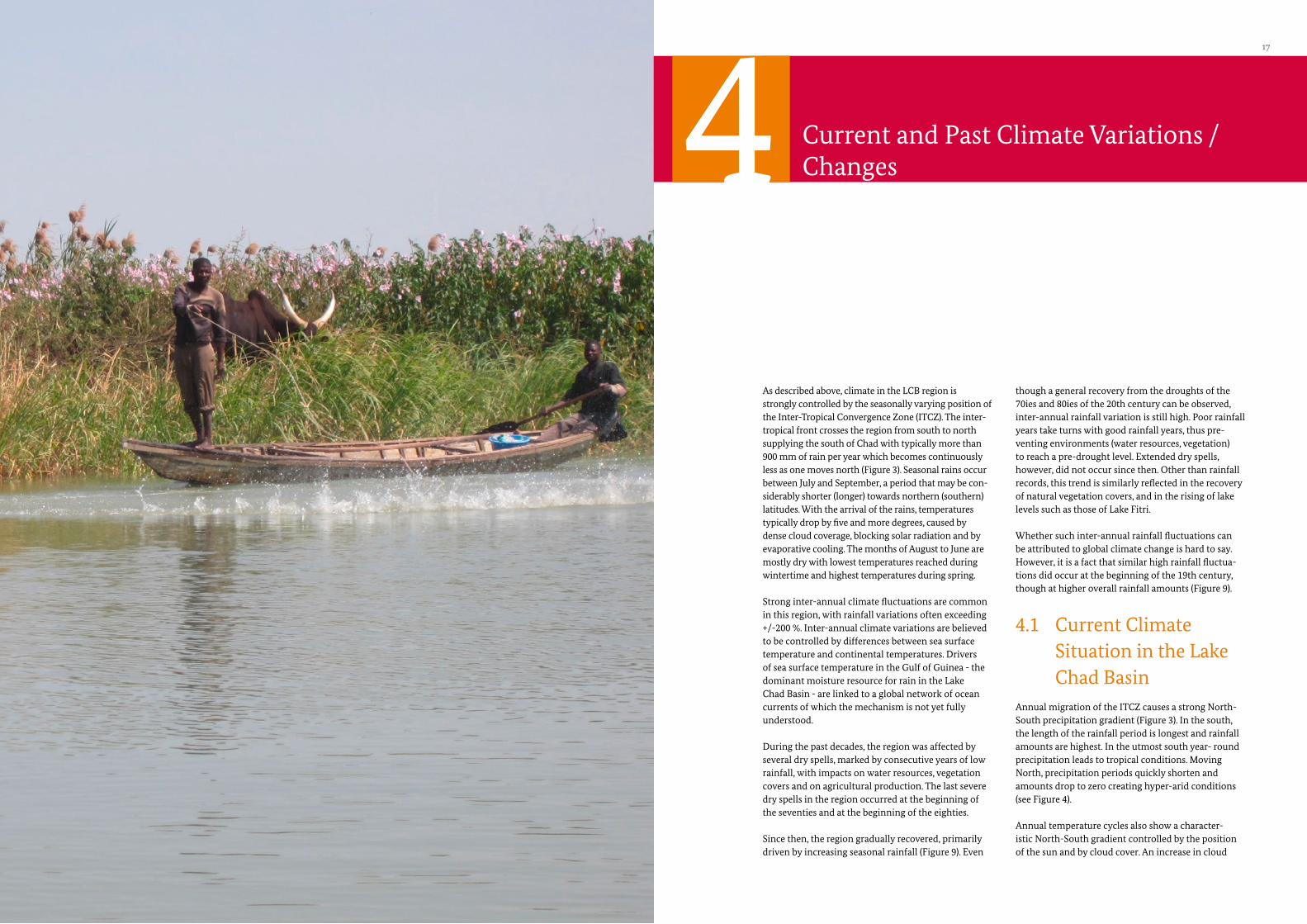
though a general recovery from the droughts of the 70ies and 80ies of the 20th century can be observed, inter-annual rainfall variation is still high. Poor rainfall years take turns with good rainfall years, thus pre-venting environments (water resources, vegetation) to reach a pre-drought level. Extended dry spells, however, did not occur since then. Other than rainfall records, this trend is similarly reflected in the recovery of natural vegetation covers, and in the rising of lake levels such as those of Lake Fitri.
Whether such inter-annual rainfall fluctuations can be attributed to global climate change is hard to say. However, it is a fact that similar high rainfall fluctua-tions did occur at the beginning of the 19th century, though at higher overall rainfall amounts (Figure 9).
4.1 Current Climate Situation in the Lake Chad Basin
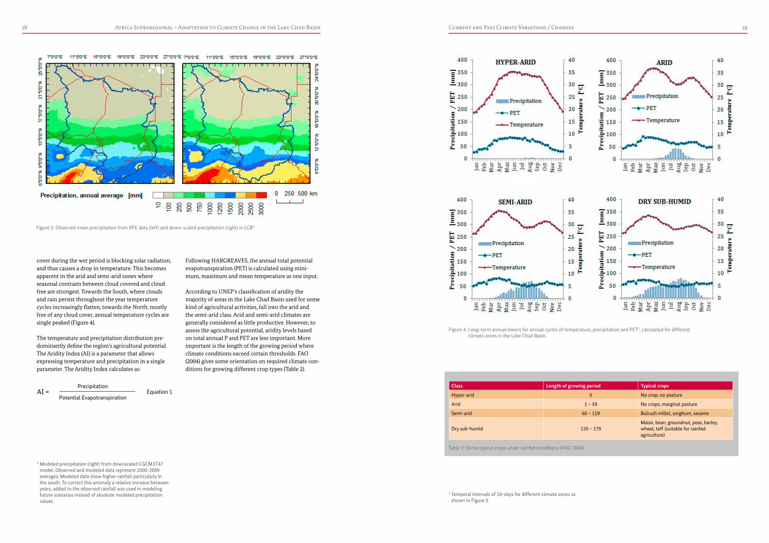
Annual migration of the ITCZ causes a strong North-South precipitation gradient (Figure 3). In the south, the length of the rainfall period is longest and rainfall amounts are highest. In the utmost south year- round precipitation leads to tropical conditions. Moving North, precipitation periods quickly shorten and amounts drop to zero creating hyper-arid conditions (see Figure 4).
Annual temperature cycles also show a character-istic North-South gradient controlled by the position of the sun and by cloud cover. An increase in cloud
As described above, climate in the LCB region is strongly controlled by the seasonally varying position of the Inter-Tropical Convergence Zone (ITCZ). The inter-tropical front crosses the region from south to north supplying the south of Chad with typically more than 900 mm of rain per year which becomes continuously less as one moves north (Figure 3). Seasonal rains occur between July and September, a period that may be con-siderably shorter (longer) towards northern (southern) latitudes. With the arrival of the rains, temperatures typically drop by five and more degrees, caused by dense cloud coverage, blocking solar radiation and by evaporative cooling. The months of August to June are mostly dry with lowest temperatures reached during wintertime and highest temperatures during spring.
Strong inter-annual climate fluctuations are common in this region, with rainfall variations often exceeding +/-200 %. Inter-annual climate variations are believed to be controlled by differences between sea surface temperature and continental temperatures. Drivers of sea surface temperature in the Gulf of Guinea - the dominant moisture resource for rain in the Lake Chad Basin - are linked to a global network of ocean currents of which the mechanism is not yet fully understood.
During the past decades, the region was affected by several dry spells, marked by consecutive years of low rainfall, with impacts on water resources, vegetation covers and on agricultural production. The last severe dry spells in the region occurred at the beginning of the seventies and at the beginning of the eighties.
Since then, the region gradually recovered, primarily driven by increasing seasonal rainfall (Figure 9). Even
Current and Past Climate Variations / Changes4
Africa Supraregional – Adaptation to Climate Change in the Lake Chad Basin18 19
Figure 3: Observed mean precipitation from RFE data (left) and down-scaled precipitation (right) in LCB4
Figure 4: Long-term annual means for annual cycles of temperature, precipitation and PET5, calculated for different climate zones in the Lake Chad Basin.
Table 2: Some typical crops under rainfed conditions (FAO, 2004)
Current and Past Climate Variations / Changes
Class Length of growing period Typical crops
Hyper-arid 0 No crop, no pasture
Arid 1 – 59 No crops, marginal pasture
Semi-arid 60 – 119 Bulrush millet, sorghum, sesame
Dry sub-humid 120 – 179Maize, bean, groundnut, peas, barley, wheat, teff (suitable for rainfed agriculture)
Following HARGREAVES, the annual total potential evapotranspiration (PET) is calculated using mini-mum, maximum and mean temperature as one input.
According to UNEP’s classification of aridity the majority of areas in the Lake Chad Basin used for some kind of agricultural activities, fall into the arid and the semi-arid class. Arid and semi-arid climates are generally considered as little productive. However, to assess the agricultural potential, aridity levels based on total annual P and PET are less important. More important is the length of the growing period where climate conditions exceed certain thresholds. FAO (2004) gives some orientation on required climate con-ditions for growing different crop types (Table 2).
cover during the wet period is blocking solar radiation, and thus causes a drop in temperature. This becomes apparent in the arid and semi-arid zones where seasonal contrasts between cloud covered and cloud free are strongest. Towards the South, where clouds and rain persist throughout the year temperature cycles increasingly flatten, towards the North, mostly free of any cloud cover, annual temperature cycles are single peaked (Figure 4).
The temperature and precipitation distribution pre-dominantly define the region’s agricultural potential. The Aridity Index (AI) is a parameter that allows expressing temperature and precipitation in a single parameter. The Aridity Index calculates as:
AI = Precipitation
Potential EvapotranspirationEquation 1
4 Modeled precipitation (right) from downscaled CGCM3T47 model. Observed and modeled data represent 2000-2009 averages. Modeled data show higher rainfall particularly in the south. To correct this anomaly a relative increase between years, added to the observed rainfall was used in modeling future scenarios instead of absolute modeled precipitation values.
5 Temporal intervals of 10-days for different climate zones as shown in Figure 5
Africa Supraregional – Adaptation to Climate Change in the Lake Chad Basin20 21
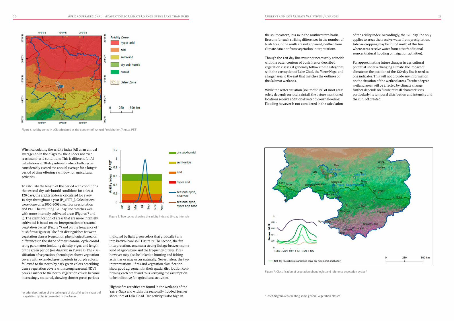
of the aridity index. Accordingly, the 120-day line only applies to areas that receive water from precipitation. Intense cropping may be found north of this line where areas receive water from other/additional sources (natural flooding or irrigation activities).
For approximating future changes in agricultural potential under a changing climate, the impact of climate on the position of the 120-day line is used as one indicator. This will not provide any information on the situation of the wetland areas. To what degree wetland areas will be affected by climate change further depends on future rainfall characteristics, particularly its temporal distribution and intensity and the run-off created.
Current and Past Climate Variations / Changes
the southeastern, less so in the southwestern basin. Reasons for such striking differences in the number of bush fires in the south are not apparent, neither from climate data nor from vegetation interpretations.
Though the 120-day line must not necessarily coincide with the outer contour of bush fires or described vegetation classes, it generally follows these categories, with the exemption of Lake Chad, the Yaere-Naga, and a larger area to the east that matches the outlines of the Salamat wetlands.
While the water situation (soil moisture) of most areas solely depends on local rainfall, the before mentioned locations receive additional water through flooding. Flooding however is not considered in the calculation
indicated by light green colors that gradually turn into brown (bare soil, Figure 7). The second, the fire interpretation, assumes a strong linkage between some kind of agriculture and the frequency of fires. Fires however may also be linked to hunting and fishing activities or may occur naturally. Nevertheless, the two interpretations – fires and vegetation classification – show good agreement in their spatial distribution con-firming each other and thus verifying the assumption to be indicative for agricultural activities.
Highest fire activities are found in the wetlands of the Yaere-Naga and within the seasonally flooded, former shorelines of Lake Chad. Fire activity is also high in
When calculating the aridity index (AI) as an annual average (An in the diagram), the AI does not even reach semi-arid conditions. This is different for AI calculations at 10-day intervals where both cycles considerably exceed the annual average for a longer period of time offering a window for agricultural activities.
To calculate the length of the period with conditions that exceed dry sub-humid conditions for at least 120 days, the aridity index is calculated for every 10 days throughout a year (P10/PET10). Calculations were done on a 2000-2009 mean for precipitation and PET. The resulting 120-day line matches well with more intensely cultivated areas (Figures 7 and 8). The identification of areas that are more intensely cultivated is based on the interpretation of seasonal vegetation cycles6 (Figure 7) and on the frequency of bush fires (Figure 8). The first distinguishes between vegetation classes (vegetation phenologies) based on differences in the shape of their seasonal cycle consid-ering parameters including density, vigor, and length of the green period (see diagram in Figure 7). The clas-sification of vegetation phenologies shows vegetation covers with extended green periods in purple colors, followed to the north by dark green colors describing dense vegetation covers with strong seasonal NDVI peaks. Further to the north, vegetation covers become increasingly scattered, showing shorter green periods
Figure 5: Aridity zones in LCB calculated as the quotient of ‘Annual Precipitation/Annual PET’
Figure 7: Classification of vegetation phenologies and reference vegetation cycles 7
Figure 6: Two cycles showing the aridity index at 10-day intervals
6 A brief description of the technique of classifying the shapes of vegetation cycles is presented in the Annex. 7 Inset diagram representing some general vegetation classes

Africa Supraregional – Adaptation to Climate Change in the Lake Chad Basin22 23
is gridded, coarse resolution (5 degrees) data provided by CRUTEM (Hadley Center). This data set contains temperature data averaged over a 5 x 5 degree area (about 600 km x 600 km) as indicated in Figure 10 and covers different periods depending on data availabil-ity (absolute earliest records start in 1850, earliest in the LCB in 1901). There are no CRUTEM data for the northeastern LCB.
The most complete records, starting at the beginning of the 20th century (western LCB), show positive tem-perature anomalies at the beginning of the century that are at a level similar or even higher than those
today. The most southern area (pixels 1407 to 1409) takes a contrasting development compared to all other areas lo-cated to the north. A mid-cen-tury temperature low visible in most northern pixels seems to correlate with a period of high rainfall (compare Figure 9). Higher cloud cover during rainy years may be one ex-planation for the temperature drop but there may be more.
beginning of 20th century, however at much lower overall rainfall amounts. The high inter-annual varia-bility makes this area and its agriculture extremely vulnerable.
4.2.2 Long-term temperature development between 1953/73 and 2013
In contrast to precipitation, no temperature data exists for this area that cover a similarly long period (1901 – present). The longest temperature data set available
Current and Past Climate Variations / Changes
form (NCDC) or pre-processed. Originally, all data are station measurements that the climate centers, for some products, interpolated to grids of different res-olution. These data sets come in resolutions of daily or monthly intervals and at spatial resolutions of 0.5 to 5 degrees. Data from the NCDC are provided as individ-ual, daily station records that can be interpolated to grids as needed.
4.2.1 Long-term precipitation development 1901 – 2010
The analyses of precipitation fluctuations and trends during the last century is based on pre-processed station data provided by the GPCC (RUDOLF et al., 2010), spatially interpolated to monthly raster data of 0.5 degree resolution. Though spatially not very detailed these data give an excellent insight into long-term regional precipitation development.
Rainfall in the LCB is submitted to pronounced inter-annual rainfall variations throughout all climate zones, which – during the observed period - only became temporarily lower (more stable) during the fifties. During this decade, the area received consis-tently high rainfall amounts. Since the nineties inter-annual variations are back to a level comparable to the
4.2 Past Climate Variation and Change
Studies of recent climate variation and change are not only a strong indicator for future climate change developments but also useful for understanding possible climate change impacts and for judging an area’s climate sensitivity. In this respect the analyses of patterns e.g. of past temperature change may be a more reliable indicator for future temperature devel-opments than results from General Circulation Models or from Regional Climate Models.
For assessing climate variation and change over the past 40 to 100 years, different precipitation and tem-perature data sets were used, provided by the Climate Research Unit Temperature (CRUTEM) of the British Hadley Climate Center, by the U.S. National Climate Data Center (NCDC) and by the Global Precipitation Climate Center (GPCC) of the Deutsche Wetterdienst (DWD).
Named centers continuously collect, store and distrib-ute data for different climate variables in their original
Figure 8: Frequency of bush fires between 2001 and 20138
Figure 9: Annual precipitation anomalies9
Figure 10: Grid displaying CRUTEM4 pixel size and location 10
8 Indicator for the distribution of some kind of agricultural (farming, fishing, hunting) activity
9 Deviation from mean between 1901 and 2010 for the arid (top) and the semi-arid climate zone of the LCB as delineated in Figure 5. Anomalies are calculated relative to a 1981-2001 mean. Mean precipitation for the arid zone and semi-arid zone is 340 mm and 860 mm resp.
10 Temperatures from available climate stations (red dots) are averaged across the pixel area. Figure 11 presents temperature diagrams (anomalies) for each pixel area. Numbers stand for the pixel Id in the CRUTEM4 grid.

Africa Supraregional – Adaptation to Climate Change in the Lake Chad Basin24 25
strong impact on water resources (soil moisture) as changes in annual temperatures suggest. In con-trast, agricultural activities extending into months of October and November are likely to struggle more with the effects of a temperature increase.
basin periphery, representing the area with maximum precipitation and hence most river discharge, temper-ature increases are among the lowest during all seasons.
As the rainy season is least affected by temperature increases, past climate change does not have such a
detailed impression on spatio-temporal variations of temperature change. Over the past 40 years, the eastern Chad experiences the highest temperature increase in the entire basin. Increases across the entire basin are strongest during spring and fall (up to 6 °C). During summer and during winter months we see the “least” temperature increases (3-4 °C). Along the southern
A spatially and temporally more detailed represen-tation of temperature development over the past decades is given in Figure 12. Trends shown in Figure 12 result from spatially interpolated daily station data obtained from the National Climate Data Center (NCDC). The results confirm the overall trends as seen in the CRUTEM data; however, the results give a more
Current and Past Climate Variations / Changes
Figure 11: Changes in annual temperature (CRUTEM4 data) in the LCB11
11 In the above map, diagrams approximately cover the area they represent (each pixel is about 600 km x 600 km, compare Figure 10).
12 Strongest temperature increases occurred during spring and fall. Colors indicate the increase per year. An increase of 0.1°C is equivalent to a 3.1°C (31 years x 0.1°C) increase between 1973 and 2013.
Figure 12: Seasonal temperature trends12

Africa Supraregional – Adaptation to Climate Change in the Lake Chad Basin26 27
two parameters, temperature and precipitation. An ensemble mean13 of the CGSM model is applied for the analysis.
5.2 Climate Change Scenarios
The international Panel on Climate Change (IPCC) has developed a set of emission scenarios that describe possible developments of different parameters with an impact on greenhouse gas concentrations. Parameters include among others population growth, economic development, and the introduction of new and more efficient technology (IPPC, 2007a; IPPC, 2007b).
From these so-called story lines, this study analyzed the B1, the A1b and the A2 scenarios. Key elements of either story line are the following: The A1 story line is marked by a very rapid
economic growth, a global population that will peak in mid-century and decline thereafter and a rapid introduction of new and more efficient technologies.
The A2 story line describes a regionally fragmented economic growth, where new technologies are introduced much slower and only locally. Population growth is con-tinuously increasing.
The B1 story line has a population growth similar as in A1, with a quicker change in economic structures toward a service and information economy, with reductions in material intensity and the introduction of clean and resource-efficient technologies.
Outputs from a range of different general circulation models (GCM) are available for the analysis of possible impacts of future climate change on natural resources of the Lake Chad Basin. This climate study considers model outputs from ocean-atmosphere coupled models only as required for a model’s consideration in the IPCC report (IPCC, 2013). Typical GCM outputs have spatial resolutions between 1.4 and 5 degrees (150 km2 to 600 km2). While detailed in their global climate forecasts, GCMs are much less accurate in the prediction of regional climate change. Only in part this is due to their coarse spatial resolution. A further reason is the complexity of processes that are not yet fully understood.
5.1 General Circulation Models (GCM)
Different GCMs perform differently well in different areas. While temperatures are usually well captured by most models they often perform much poorer in the projection of future precipitation. The model outputs for a reference period (observed period), usually the period between 1990 and 2000, provide guidance for the performance of a distinct model in an area of interest. The outputs of three different GCMs were ex-amined that included those from the American CCSM model, the Canadian CGSM model and the British HadGEM1. The CGSM data from the Canadian Climate Change Scenarios Network (CCCSN) best describe the
Future Climate Change5
13 As starting climate conditions are unknown, model runs are typically initiated using different starting conditions (usually seven runs). An ensemble is the total number of model runs.

Africa Supraregional – Adaptation to Climate Change in the Lake Chad Basin28 29
ature increase during summer (main cropping season) and winter. Areas of highest temperature increase within the water productive basin are the eastern (area of Abeche) and the central Lake Chad Basin (see spring and fall panel in Figure14 to 16).
Spatio-temporal analyses of temperature devel-opment over the next hundred years (Figure 14 to 16) is in agreement with observed temperature changes between 1973 and 2013 (Figure 12), with change sce-narios (B1, A1b and A2) showing highest temperature increase during spring and fall and the least temper-
Future Climate Change
Temperature increase is highest in the arid (Figure 13, top) and lowest in the dry sub-humid zone (Figure 13, bottom). The high inter-annual temperature variation in the arid zone is related to inter-annual variations in cloud cover that are less pronounced in the semi-arid and dry sub-humid zone.
Increasing temperature will lift water losses through eva-potranspiration. A rough approximation for assessing the water loss to evapotranspiration is as follows: Each 1 °C increase in temperature will increase evapotranspiration by about 0.4 mm per day. Assuming sufficient soil mois-ture will be available for about 120 days, the additional water loss amounts to 48 mm. However, the exact amount will further depend on variables such as vegetation cover, wind speed, air humidity and soils.
5.3 Data PreparationBecause of the coarse spatial (3.7 degrees) and temporal (monthly) resolution of the CGSM products, they have only little meaning at a local scale. Therefore both climate parameters are downscaled to 10-day intervals and 5 km (temperature) and 12 km (precipi-tation) respectively (WILBY et al., 1998). The process of downscaling relies on statistical relationships that are in case of temperature linkages between topographic elevation and temperature (lapse rate), in the case of precipitation observed precipitation distribution patterns that are applied to future change scenario data. This assumes that observed statistical relation-ships do not change over time.
For the downscaling of temperature, the 1 km resolv-ing GMTED2010 data and a lapse rate of 5 °C are used. For precipitation, statistics of spatial and temporal patterns were derived from 12 km resolving RFE data (LAWS et al., 2004). For both parameters, data covering the period from 2000 to 2099 were processed.
5.4 Climate Change under Different Scenarios
Where data processing times and data evaluation were within a manageable amount, results are presented for all three scenarios (B1, A1b and A2, e.g. parameter tem-perature). However, where time consuming processing steps are required the focus of the study was on the B1 and the A2 scenario (rainfall, various modeled, hydro-meteorological parameters). Time intervals at which future change situations are presented may vary, depending on the magnitude of change that occurs between two points in time.
5.4.1 TemperatureThe B1 story line represents the mildest temper-ature increase of the discussed scenarios. In a B1 scenario, annual average temperatures will increase until the end of the century by an approximate 2 °C, plus/minus 0.5 °C depending on the climate zone. A significant difference in temperature increase between different scenarios does not occur before the end of the 2030ies. Latest at the beginning of 2040 in an A1b and an A2 scenario, temperatures will start increasing faster resulting in a total temperature increase of 3 °C (A1b) and 4 °C (A2) by 2099.
It is worthwhile to mention that future temperature increases over the next 100 years are expected to be considerably lower than the increases observed between 1974 and 2013.
14 According to different climate change scenarios and for different aridity zones: arid (top), semi-arid (middle) and dry sub-humid (bottom)
15 According to CGSM data (CGCM3T47) from the Canadian Climate Change Scenarios Network (CCCSN). Note that color scale is not comparable with Figure 12 showing temperature changes between 1973 and 2013, due to large scale differ-ences (~4°C/40years compared to ~2.4°C/100years).
Figure 13: Temperature change between 2000 and 209914
Figure 14: Seasonal temperature change under a B1 scenario15

Africa Supraregional – Adaptation to Climate Change in the Lake Chad Basin30 31Future Climate Change
16 According to CGSM data (CGCM3T47) from the Canadian Climate Change Scenarios Network (CCCSN). Note, color scale is not comparable with Figure 14 showing temperature changes between 1973 and 2013, due to large scale differ-ences (~4°C/40years compared to ~2.4°C/100years).
17 According to CGSM data (CGCM3T47) from the Canadian Climate Change Scenarios Network (CCCSN). Note, color scale is not comparable with Figure 14 showing temper-ature changes between 1973 and 2013, due to large scale differences (~4°C/40years compared to ~2.4°C/100years).
Figure 15: Seasonal temperature change under an A1b scenario 16 Figure 16: Seasonal temperature change under an A2 scenario17
Africa Supraregional – Adaptation to Climate Change in the Lake Chad Basin32 33Future Climate Change
nual AI is little meaningful. Rainfall is concentrated on a few months during which it is crucial for how long the AI exceeds a threshold that is considered favorable for growing distinct crops (Table 2). Accordingly, the AI was calculated for every 10-day interval and the duration the AI exceeded dry sub-humid conditions was derived thereof. A minimum duration of 120 days under dry sub-humid conditions is required to grow crops as listed in Table 2. A mean 120-day line, con-structed from AI values averaged over years 2000-2013, is used as a baseline against which future changes are measured.
The average 120-day line, well describes the beginning of intense, rainfed cultivation in the Basin. The line is solely based on temperature – or rather PET derived thereof - and the distribution of local precipitation. Where areas receive additional water from other sources, intense cultivation may be possible beyond this line, particularly in wetlands like the Yaere-Naga,
5.5 Impact of Climate Change on the Length of the Growing Period
For monitoring the impact of projected climate change on agricultural potentials (IMPACT ASSESS-MENT INC., 2006), the parameter Aridity Index (AI) is used (Equation 1). The AI combines precipitation and temperature in one variable. Due to no rainfall and high temperatures throughout most of the year, an an-
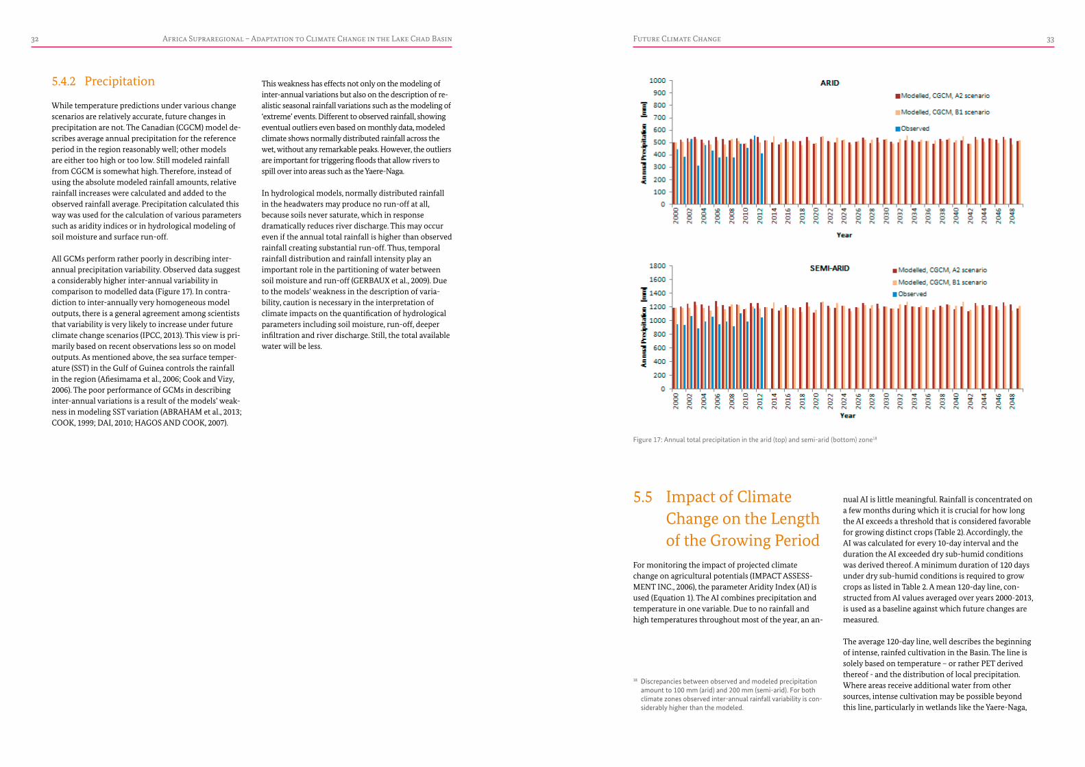
This weakness has effects not only on the modeling of inter-annual variations but also on the description of re-alistic seasonal rainfall variations such as the modeling of ‘extreme’ events. Different to observed rainfall, showing eventual outliers even based on monthly data, modeled climate shows normally distributed rainfall across the wet, without any remarkable peaks. However, the outliers are important for triggering floods that allow rivers to spill over into areas such as the Yaere-Naga.
In hydrological models, normally distributed rainfall in the headwaters may produce no run-off at all, because soils never saturate, which in response dramatically reduces river discharge. This may occur even if the annual total rainfall is higher than observed rainfall creating substantial run-off. Thus, temporal rainfall distribution and rainfall intensity play an important role in the partitioning of water between soil moisture and run-off (GERBAUX et al., 2009). Due to the models’ weakness in the description of varia-bility, caution is necessary in the interpretation of climate impacts on the quantification of hydrological parameters including soil moisture, run-off, deeper infiltration and river discharge. Still, the total available water will be less.
5.4.2 Precipitation
While temperature predictions under various change scenarios are relatively accurate, future changes in precipitation are not. The Canadian (CGCM) model de-scribes average annual precipitation for the reference period in the region reasonably well; other models are either too high or too low. Still modeled rainfall from CGCM is somewhat high. Therefore, instead of using the absolute modeled rainfall amounts, relative rainfall increases were calculated and added to the observed rainfall average. Precipitation calculated this way was used for the calculation of various parameters such as aridity indices or in hydrological modeling of soil moisture and surface run-off.
All GCMs perform rather poorly in describing inter-annual precipitation variability. Observed data suggest a considerably higher inter-annual variability in comparison to modelled data (Figure 17). In contra-diction to inter-annually very homogeneous model outputs, there is a general agreement among scientists that variability is very likely to increase under future climate change scenarios (IPCC, 2013). This view is pri-marily based on recent observations less so on model outputs. As mentioned above, the sea surface temper-ature (SST) in the Gulf of Guinea controls the rainfall in the region (Afiesimama et al., 2006; Cook and Vizy, 2006). The poor performance of GCMs in describing inter-annual variations is a result of the models’ weak-ness in modeling SST variation (ABRAHAM et al., 2013; COOK, 1999; DAI, 2010; HAGOS AND COOK, 2007).
18 Discrepancies between observed and modeled precipitation amount to 100 mm (arid) and 200 mm (semi-arid). For both climate zones observed inter-annual rainfall variability is con-siderably higher than the modeled.
Figure 17: Annual total precipitation in the arid (top) and semi-arid (bottom) zone18
Africa Supraregional – Adaptation to Climate Change in the Lake Chad Basin34 35Future Climate Change
(within which the 120-day line fluctuates) cannot be calculated from the GCM data, as models only poorly describe inter-annual rainfall variability. Although, current fluctuations of the 120-day line exceed the magnitude of retreat under both, a B1 and an A2 scenario, future fluctuations may even be larger and increase the risk for droughts.
A time-series of more detailed maps for a B1 and an A2 scenario, with further sub-divisions for the length of the growing period is presented in Chapter 7. The time-series visualizes spatially distributed effects of climate change on the Aridity Index. E.g., the transition from arid to hyper-arid conditions remains almost unaffected under either change scenario and has little impact on the location of the arid to semi-arid boundary.
Impacts of climate change tend to become continu-ously larger – causing larger displacements of bound-aries – as one moves south, towards longer growing periods. Classes 201-203 (growing days) and 231-260, approximately covering areas with tropical conditions, become increasingly fragmented or disappear (231-260 class). Climate conditions supporting the growth of tropical forests may no longer exist in these areas at the end of the century.
may be different as they are further controlled by groundwater and do not instantly respond to inter-annual rainfall variation. Generally, tree vegetation gradually increases to the south, e.g. as shown by continuously lower correlations between precipitation and biomass. The present situation of aquifers, includ-ing ground water levels/variations, flow and replenish-ment are still under investigation. A completion of this study will be a pre-condition for drawing meaningful conclusions on the impact of future climate change scenarios on groundwater.
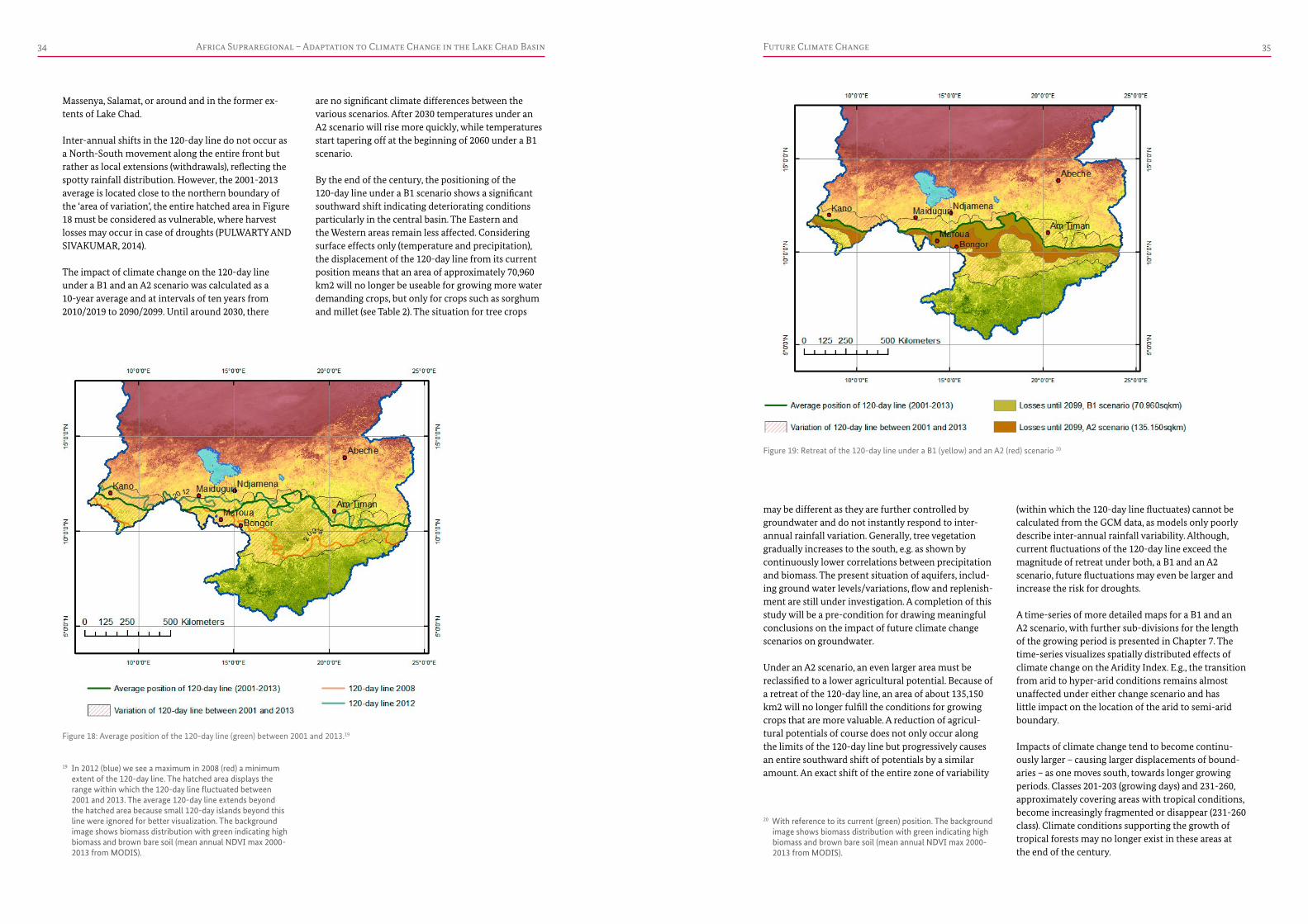
Under an A2 scenario, an even larger area must be reclassified to a lower agricultural potential. Because of a retreat of the 120-day line, an area of about 135,150 km2 will no longer fulfill the conditions for growing crops that are more valuable. A reduction of agricul-tural potentials of course does not only occur along the limits of the 120-day line but progressively causes an entire southward shift of potentials by a similar amount. An exact shift of the entire zone of variability
are no significant climate differences between the various scenarios. After 2030 temperatures under an A2 scenario will rise more quickly, while temperatures start tapering off at the beginning of 2060 under a B1 scenario.
By the end of the century, the positioning of the 120-day line under a B1 scenario shows a significant southward shift indicating deteriorating conditions particularly in the central basin. The Eastern and the Western areas remain less affected. Considering surface effects only (temperature and precipitation), the displacement of the 120-day line from its current position means that an area of approximately 70,960 km2 will no longer be useable for growing more water demanding crops, but only for crops such as sorghum and millet (see Table 2). The situation for tree crops
Massenya, Salamat, or around and in the former ex-tents of Lake Chad.
Inter-annual shifts in the 120-day line do not occur as a North-South movement along the entire front but rather as local extensions (withdrawals), reflecting the spotty rainfall distribution. However, the 2001-2013 average is located close to the northern boundary of the ‘area of variation’, the entire hatched area in Figure 18 must be considered as vulnerable, where harvest losses may occur in case of droughts (PULWARTY AND SIVAKUMAR, 2014).
The impact of climate change on the 120-day line under a B1 and an A2 scenario was calculated as a 10-year average and at intervals of ten years from 2010/2019 to 2090/2099. Until around 2030, there
19 In 2012 (blue) we see a maximum in 2008 (red) a minimum extent of the 120-day line. The hatched area displays the range within which the 120-day line fluctuated between 2001 and 2013. The average 120-day line extends beyond the hatched area because small 120-day islands beyond this line were ignored for better visualization. The background image shows biomass distribution with green indicating high biomass and brown bare soil (mean annual NDVI max 2000-2013 from MODIS).
20 With reference to its current (green) position. The background image shows biomass distribution with green indicating high biomass and brown bare soil (mean annual NDVI max 2000-2013 from MODIS).
Figure 18: Average position of the 120-day line (green) between 2001 and 2013.19
Figure 19: Retreat of the 120-day line under a B1 (yellow) and an A2 (red) scenario 20
Africa Supraregional – Adaptation to Climate Change in the Lake Chad Basin36 37Future Climate Change
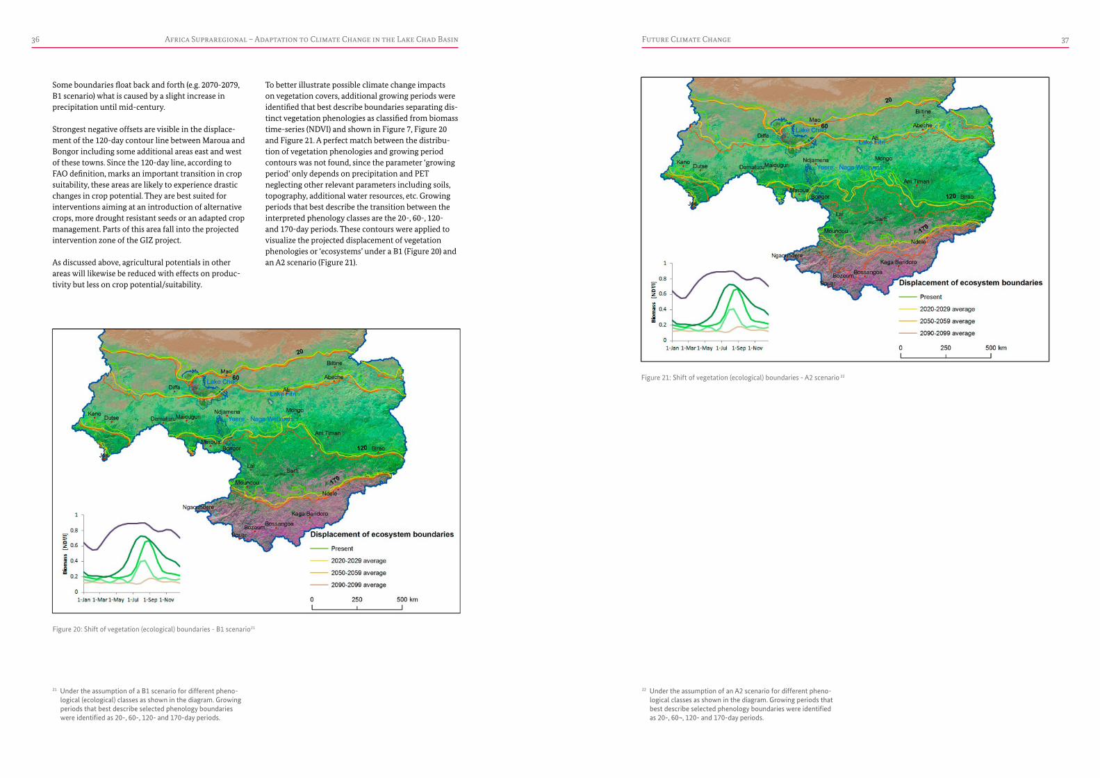
To better illustrate possible climate change impacts on vegetation covers, additional growing periods were identified that best describe boundaries separating dis-tinct vegetation phenologies as classified from biomass time-series (NDVI) and shown in Figure 7, Figure 20 and Figure 21. A perfect match between the distribu-tion of vegetation phenologies and growing period contours was not found, since the parameter ‘growing period’ only depends on precipitation and PET neglecting other relevant parameters including soils, topography, additional water resources, etc. Growing periods that best describe the transition between the interpreted phenology classes are the 20-, 60-, 120- and 170-day periods. These contours were applied to visualize the projected displacement of vegetation phenologies or ‘ecosystems’ under a B1 (Figure 20) and an A2 scenario (Figure 21).
Some boundaries float back and forth (e.g. 2070-2079, B1 scenario) what is caused by a slight increase in precipitation until mid-century.
Strongest negative offsets are visible in the displace-ment of the 120-day contour line between Maroua and Bongor including some additional areas east and west of these towns. Since the 120-day line, according to FAO definition, marks an important transition in crop suitability, these areas are likely to experience drastic changes in crop potential. They are best suited for interventions aiming at an introduction of alternative crops, more drought resistant seeds or an adapted crop management. Parts of this area fall into the projected intervention zone of the GIZ project.
As discussed above, agricultural potentials in other areas will likewise be reduced with effects on produc-tivity but less on crop potential/suitability.
Figure 20: Shift of vegetation (ecological) boundaries - B1 scenario21
Figure 21: Shift of vegetation (ecological) boundaries - A2 scenario 22
21 Under the assumption of a B1 scenario for different pheno-logical (ecological) classes as shown in the diagram. Growing periods that best describe selected phenology boundaries were identified as 20-, 60-, 120- and 170-day periods.
22 Under the assumption of an A2 scenario for different pheno-logical classes as shown in the diagram. Growing periods that best describe selected phenology boundaries were identified as 20-, 60¬, 120- and 170-day periods.

Africa Supraregional – Adaptation to Climate Change in the Lake Chad Basin38 39
charge characteristics of the Logone River. Located at the former estuary of the Palaeo Logone into Lake Mega Chad (Figure 22), the flat morphology causes a slowdown of flow velocity, triggering the accumula-tion of river sediments and a spillover of river waters into adjacent areas.
The Naga-Yaere Wetlands are a seasonally flooded area of roughly 7,500 km2 and located within the semi-arid climate zone. Annual rainfall amount in the Yaere-Naga wetlands is between 600 and 800 mm. The vegetation of the wetlands shows growing periods that are significantly longer than in its surrounding areas.
With evapotranspiration rates of around 430 mm between July and September and more than 1,000 mm until the end of the year (annual total about 2,400 mm), local rainfall is far from being sufficient to support such growth periods. During summer time, spillovers of the Logone River into the wetlands, con-tribute an estimated equivalent of about 900 mm of rainfall to the Yaere–Naga wetlands (400 mm during dry years). These numbers result from evaluations of river discharge measurements, showing downstream discharge losses as the Logone passes the Yaere-Naga wetlands (Figure 22). River water discharges into the Yaere-Naga through natural pathways and through man-made canals constructed for fishing (canaux de pêches). The floodwater supports an extended growing period of (natural) vegetation cover that may be 3 to 4 months longer than in areas outside the Yaere-Naga.
While this potential is rarely exploited for extended farming activities, it represents a fodder resource for animals, for fishing and for replenishing groundwater. Larger irrigation schemes inside the Yaere-Naga such as those at Lake Maga and near Logone-gana do not depend on inundations. To sustain multiple crops these schemes draw water directly from the Maga reservoir or from the Logone River.
The Yaere-Naga owes its particular situation of seasonal flooding to its smooth morphology and dis-
Yaere – Naga Wetlands6
Figure 22: Geomorphological setting of the Yaere-Naga wetlands 23
23 At the former estuary of the Logone River into Lake Mega Chad (former shore line of Lake Mega Chad shown as brown lines).

Africa Supraregional – Adaptation to Climate Change in the Lake Chad Basin40 41
The model results however do not allow distinguish-ing between losses to soil moisture, deeper infiltration water and run-off. Though hydrologic modeling suggests dramatic run-off losses (see Chapter 7.5), these losses bear little credibility due to the weak-nesses in GCM data.
One has to assume, however that flooding of the Yaere-Naga wetlands is likely to happen only at a lesser extent, and even if flooding continues at the current level, increasing evaporation rates will shorten the period with abundant soil moisture.
In order to understand the impact of these influences on the situation of the Yaere-Naga wetlands, a compar-ison of two vegetation classifications during a wet and a dry year was undertaken. The results of this analysis are presented in Figure 27.
Yaere – Naga Wetlands
istic highlights the importance of upstream rainfall distribution and rainfall intensity. As the GCP model data do not adequately capture these two parameters, meaningful analyses for future change scenarios are not possible.
Flatness of the curve is a matter of soil characteristics and particularly of its water holding capacity and infiltration rate. Once the water holding capacity of the soil is reached, any additional water (precipitation) creates run-off. The vertical spread of points in Figure 25 is an expression of varying rainfall intensities and timing. E.g., a short lasting but intense rainfall event may quickly lead to soil saturation and to the creation of surface run-off, while long lasting or repeated events of low intensity may never reach a point of sat-uration, creating no run-off at all.
As discussed under 5.4.2, future rainfall characteristics (intensity and timing and spatial distribution), there-fore are critical in determining future surface run-off and possible flooding scenarios of the Yaere-Naga wetlands. Rainfall intensity and timing are however, poorly described in general circulation models due to physical model limitations and their spatial (several 100 km2) and temporal resolution (monthly).
The above can be approximated with some confidence for the total water losses to evaporation, at the expense of soil moisture, deeper infiltration and run-off as a whole. Soil moisture, deeper infiltration and surface run-off have been obtained from hydrologic model calculations. Projected water losses in the effective run-off area of the Logone River amount to 4 % under a B1 scenario (up to 9 % under an A1 scenario) until 2099 (Figure 26).
respectively. The intercept of the trendline with the x-axis at 356 m3/sec (1,055 m3/sec) marks the begin-ning of the spillover into the Yaere wetlands between Bongor and Katoa. To calculate or forecast temporal development of water losses, e.g. to forecast flooding extent and severity, the equation in Figure 24 (left) applies for Bongor discharge rates between 356 to 1,055 m3/sec, the equation in Figure 24 (right) applies for Bongor discharge rates greater 1,055 m3/sec. The calculation of the relationship between discharge and outflow is based on river discharge records between 2001 and 2005 and shows a strong linearity. This line-arity must not necessarily apply for higher discharge rates.
The observed relationship between Bongor discharge and spillover into the Yaere, shows that total dis-charge is insignificant compared to the magnitude and frequency of discharge peaks exceeding described thresholds. The diagrams in Figure 24 suggest that without exceeding defined discharge thresholds no spillover into the wetlands will occur. This character-
Depending on river discharge at Bongor the Logone river is losing water as far downstream as Logone-gana. The outflow into the Yaere wetlands (greyish area in Figure 23) between Katoa and Logone-gana starts, once discharge rates at Bongor exceed about 356 m3/sec; between Bongor and Katoa outflow starts when discharge rates exceed 1,055 m3 (Bongor station). As the diagram in Figure 23 shows, there is some return flow between Katoa and Logone-gana during November and December (crossover of discharge curves).
Figure 24 summarizes water losses of the Logone River between Bongor and Katoa with discharge rates at Bongor plotted against water losses to the Yaere between Bongor-Katoa and between Katoa-Logone
Figure 23: River discharge at Bongor, Katoa and Logone-gana stations 24 Figure 25: Correlation between rainfall in the Bongor catchment and river discharge measured at Bongor 26
Figure 26: Total water losses in the effective run-off area of the Logone River. 27
Figure 24: Discharge thresholds for Logone water losses 25
24 Listed in downstream order, showing down-stream water losses of the Logone River.
25 Between Katoa and Logone-gana (left) and between Bongor and Katoa (right) 26 Blue lines indicate outflow thresholds into the Yaere-Naga
27 Total water losses are calculated as the sum of losses in soil moisture, deeper infiltration water and run-off water.

Africa Supraregional – Adaptation to Climate Change in the Lake Chad Basin42 43
larger river courses. Otherwise, it is only man-made canals extending into these areas. From the eastern banks of the Logone River a dense network of fishing canals, several kilometers in length, diverts water into the hinterland. No farming activities were detected in these areas. In contrast, along a branch of the Logone, intense farming activities occur but only few traces of fishing canals. Apart from accessibility, morphology and flooding intensity are the major controls for farming, fishing and settlements.
6.1 Lake ChadLake Chad receives most of its water from the Chari and Logone rivers with only minor contributions from the Komadugu-Yobe River. Figure 29 presents the annual total inflow from Chari and Logone rivers into Lake Chad. Ungauged inflow to the lake coming from e.g. the El Beid River and other intermittent flow paths fed by the Yaere-Naga flood plains, contribute an additional, unknown volume of water. A rising PET in the headwaters will similarly reduce the total water available, as described for the Yaere-Naga wetlands, with effects on river discharge. Total upstream water losses range between 4 % and 10 % of the currently available water. Again, a quantification of future dis-charge reduction is not possible, since GCM data do not allow reliable modeling of water partitioning among soil moisture, deeper infiltration and surface run-off.
Yaere – Naga Wetlands
at the eastern periphery of the wetlands that can better preserve soil moisture (dark green areas north of Lake Maga).
The changes east of the Yaere-Naga with Phen Cl2 turning into Phen Cl3, (Figure 27, left diagram) towards a much shorter green period, illustrate the vulnerability of these areas. Areas south of Lake Maga and roughly coinciding with the 120-day line (see Figures 20 and 21) appear less sensitive to climate vari-ation.
People in the Yaere-Naga wetlands seem to be aware of this situation and concentrate their activities on these core areas of inundation (Figure 28). However, it needs to be mentioned that only few areas have been inter-preted for the distribution of settlements and activities due to the limited availability of high-resolution satellite data.
Settlements and associated small-scale farming activities are only found near the course of main rivers (Logone and its branches). As satellite analyses suggest farmers grow one crop per year only. Moving away from the main river, settlements and farming activities disappear, unless they are accessible through
Maga in the south; red colors irrigated double crops. The project intervention zone is outlined in red; drainage patterns interpreted from pan-sharpened Landsat data (10 m resolution) are presented in blue. Coloring of reference cycles matches their respective class in the classifications.
Conceivable scenarios are controlled by morphology and drainage pattern affecting the extent of flooding. This may result in an increased fragmentation of flooded areas or a simple shrinking towards a center of flooding. The comparison between an observed wet and dry year does not fully satisfy the situation of climate change, since changes between the ob-served extremes are primarily driven by differences in rainfall but not by an increase in temperature. Overall, as the comparison shows, reduced flooding will cause shrinking of the wetlands. There are also some centers
The diagrams show selected reference vegetation cycles used in both classifications. During the clas-sification, pixels are identified that match the shape of the reference cycles. The dominant class during a dry year (Figure 27, left) is a phenology with a rather short green period (Phen. Cl2) that only appears in the very north during a wet period. During wet years, areas become increasingly flooded (all blue colors). Variation in blue colors is an expression of the length of flooding intensity and period (see biomass drop of bluish curves around September, right diagram). Dark green colors are representing cycles with extended green periods, light green colors stand for short green periods. Black colors are water, Lake Chad in the north and Lake
Figure 27: Classification of vegetation cycles (phenology) 28
Figure 28: Spatial distribution of human activities 29
28 Using MODIS NDVI 16-day interval time-series, showing the Yaere-Naga wetlands during a dry (2009) and a wet (2012) year.
29 Settlements, fields and fishing canals in an area within the Yaere-Naga wetlands (light green area in the location map to the right). Interpretations are based on detailed high- resolution satellite data.
Africa Supraregional – Adaptation to Climate Change in the Lake Chad Basin44 45Yaere – Naga Wetlands
values thus leave the possibility of a restoration of the lake within its 1963 shorelines doubtful, even if mod-eled rainfall data are not entirely correct.
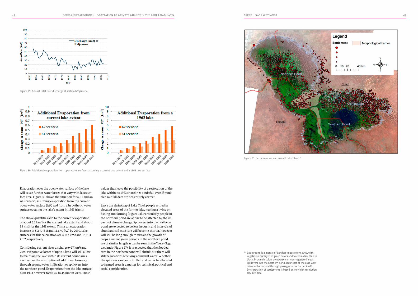
Since the shrinking of Lake Chad, people settled in elevated areas of the former lake, making a living on fishing and farming (Figure 31). Particularly people in the northern pond are at risk to be affected by the im-pacts of climate change. Spillovers into the northern pond are expected to be less frequent and intervals of abundant soil moisture will become shorter, however will still be long enough to sustain the growth of crops. Current green periods in the northern pond are of similar length as can be seen in the Yaere-Naga wetlands (Figure 27). It is expected that the flooded area in the northern pond will shrink, but there will still be locations receiving abundant water. Whether the spillover can be controlled and water be allocated to farmed areas is a matter for technical, political and social consideration.
Evaporation over the open water surface of the lake will cause further water losses that vary with lake sur-face area. Figure 30 shows the situation for a B1 and an A2 scenario, assuming evaporation from the current open water surface (left) and from a hypothetic water surface equaling the lake’s extent in 1963 (right).
The above quantities add to the current evaporation of about 5.2 km3 for the current lake extent and about 39 km3 for the 1963 extent. This is an evaporation increase of 5.2 % (B1) and 11.6 %, (A2) by 2099. Lake surfaces for this calculation are 2,142 km2 and 15,753 km2, respectively.
Considering current river discharge (~27 km3) and 2099 evaporative losses of up to 6 km3 will still allow to maintain the lake within its current boundaries, even under the assumption of additional losses e.g. through groundwater infiltration or spillovers into the northern pond. Evaporation from the lake surface as in 1963 however totals 42 to 45 km3 in 2099. These
Figure 29: Annual total river discharge at station N’djamena
Figure 31: Settlements in and around Lake Chad. 30
Figure 30: Additional evaporation from open water surfaces assuming a current lake extent and a 1963 lake surface
30 Background is a mosaic of Landsat images from 2003, with vegetation displayed in green colors and water in dark blue to black. Brownish colors are sparsely or non-vegetated areas. Spillovers into the northern pond occur east of the east-west oriented barrier and through passages in the barrier itself. Interpretation of settlements is based on very high resolution satellite data.
Africa Supraregional – Adaptation to Climate Change in the Lake Chad Basin46 47
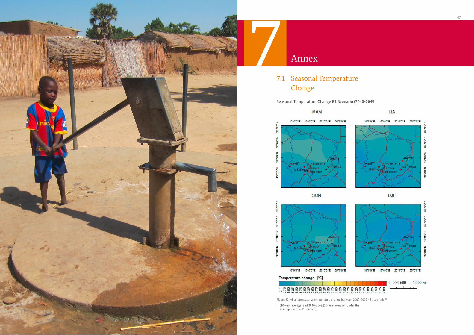
7.1 Seasonal Temperature Change
Seasonal Temperature Change B1 Scenario (2040-2049)
Annex7
Figure 32: Absolute seasonal temperature change between 2000-2009 - B1 scenario 31
31 (10-year average) and 2040-2049 (10-year average), under the assumption of a B1 scenario.
Africa Supraregional – Adaptation to Climate Change in the Lake Chad Basin48 49Annex
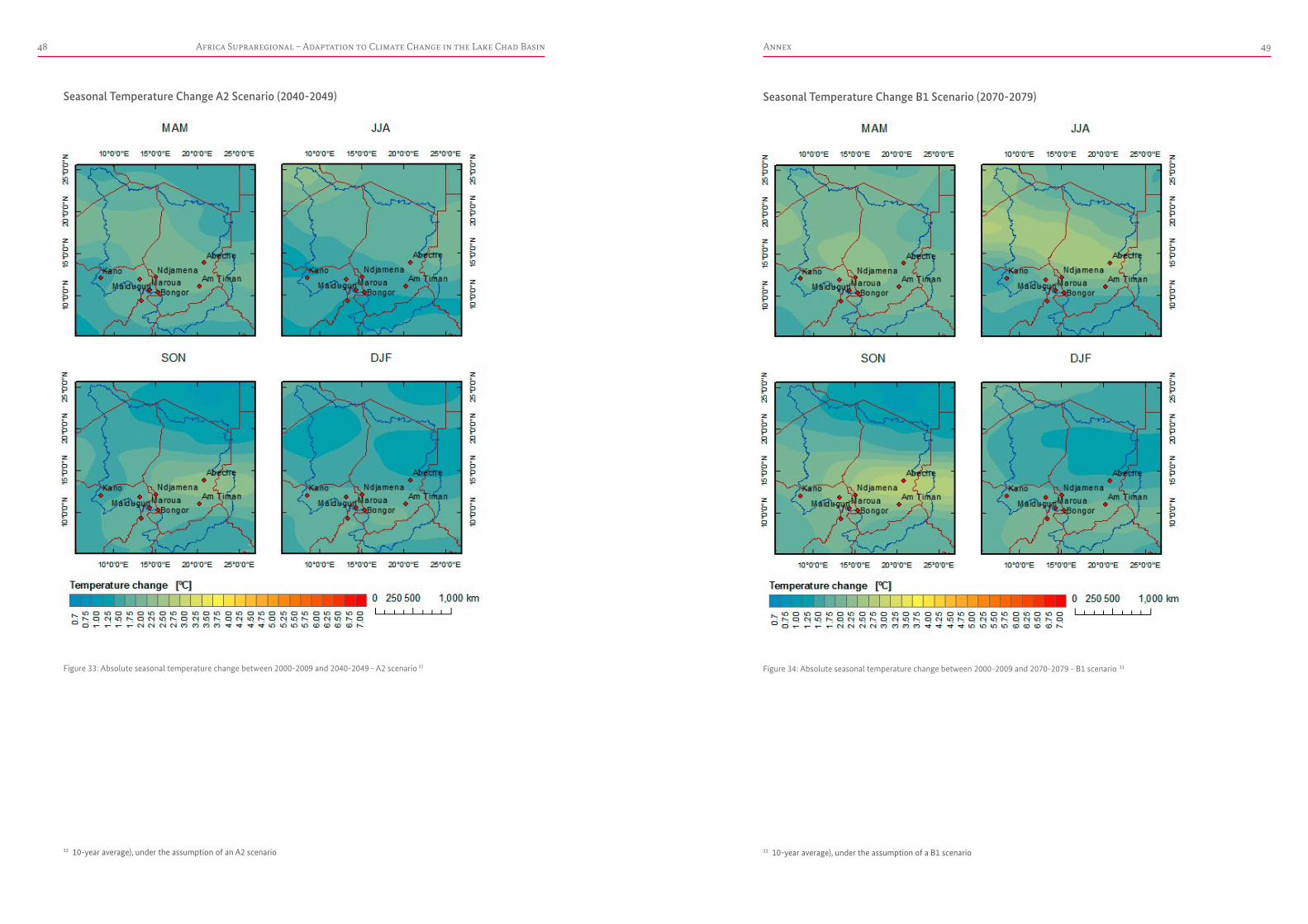
Seasonal Temperature Change A2 Scenario (2040-2049) Seasonal Temperature Change B1 Scenario (2070-2079)
Figure 33: Absolute seasonal temperature change between 2000-2009 and 2040-2049 - A2 scenario 32 Figure 34: Absolute seasonal temperature change between 2000-2009 and 2070-2079 - B1 scenario 33
32 10-year average), under the assumption of an A2 scenario 33 10-year average), under the assumption of a B1 scenario
Africa Supraregional – Adaptation to Climate Change in the Lake Chad Basin50 51Annex
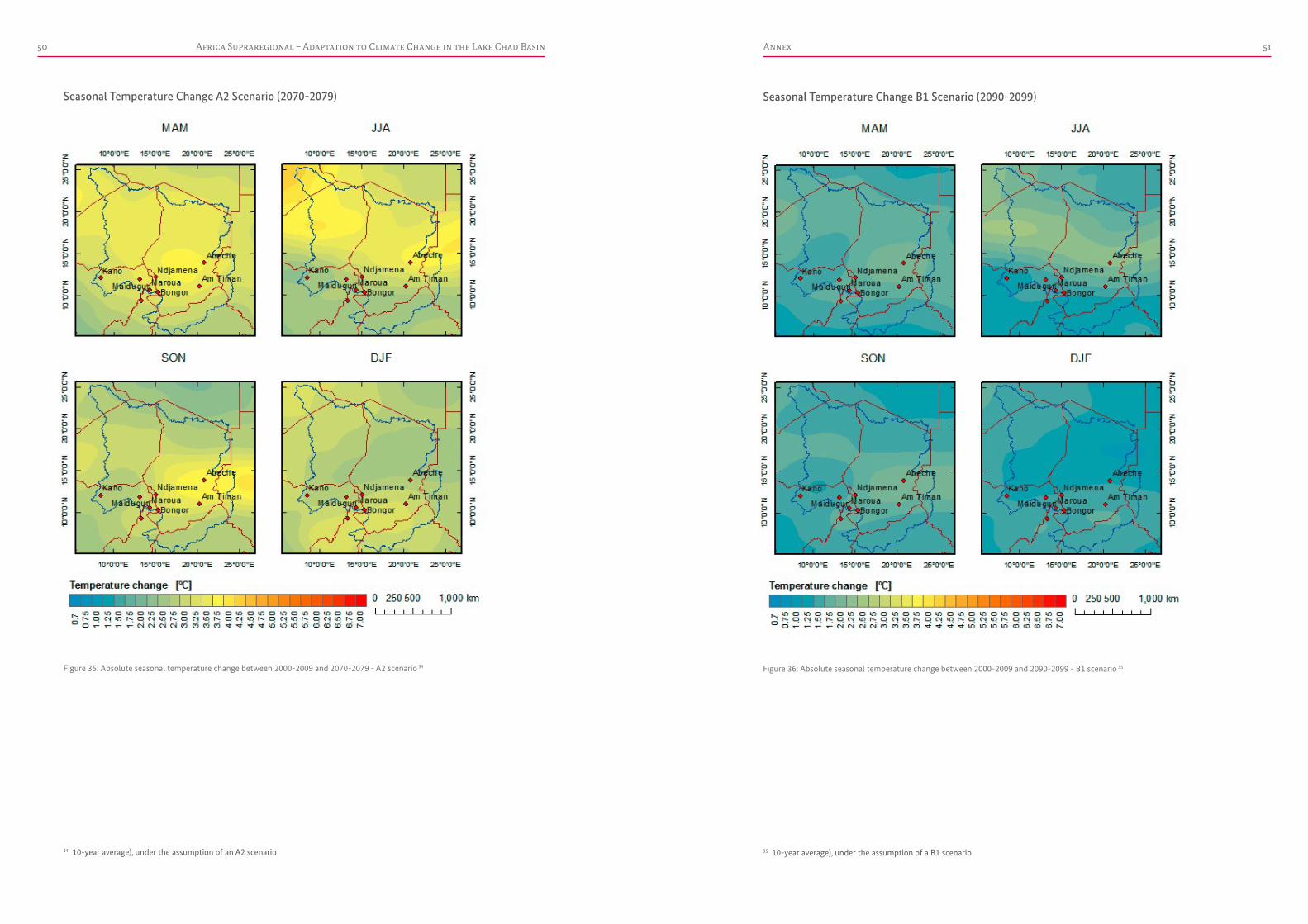
Seasonal Temperature Change A2 Scenario (2070-2079) Seasonal Temperature Change B1 Scenario (2090-2099)
Figure 35: Absolute seasonal temperature change between 2000-2009 and 2070-2079 - A2 scenario 34 Figure 36: Absolute seasonal temperature change between 2000-2009 and 2090-2099 - B1 scenario 35
34 10-year average), under the assumption of an A2 scenario 35 10-year average), under the assumption of a B1 scenario
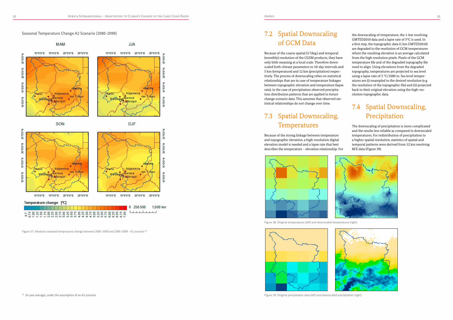
Africa Supraregional – Adaptation to Climate Change in the Lake Chad Basin52 53
the downscaling of temperature, the 1-km resolving GMTED2010 data and a lapse rate of 5°C is used. In a first step, the topographic data (1 km GMTED2010) are degraded to the resolution of GCM temperatures where the resulting elevation is an average calculated from the high resolution pixels. Pixels of the GCM temperature file and of the degraded topography file need to align. Using elevations from the degraded topography, temperatures are projected to sea level using a lapse rate of 5 °C/1000 m. Sea level temper-atures are (i) resampled to the desired resolution (e.g. the resolution of the topographic file) and (ii) projected back to their original elevation using the high-res-olution topographic data.
7.4 Spatial Downscaling, Precipitation
The downscaling of precipitation is more complicated and the results less reliable as compared to downscaled temperatures. For redistribution of precipitation to a higher spatial resolution, statistics of spatial and temporal patterns were derived from 12 km resolving RFE data (Figure 39).
7.2 Spatial Downscaling of GCM Data
Because of the coarse spatial (3.7deg.) and temporal (monthly) resolution of the CGSM products, they have only little meaning at a local scale. Therefore down-scaled both climate parameters to 10-day intervals and 5 km (temperature) and 12 km (precipitation) respec-tively. The process of downscaling relies on statistical relationships that are in case of temperature linkages between topographic elevation and temperature (lapse rate), in the case of precipitation observed precipita-tion distribution patterns that are applied to future change scenario data. This assumes that observed sta-tistical relationships do not change over time.
7.3 Spatial Downscaling, Temperatures
Because of the strong linkage between temperature and topographic elevation, a high-resolution digital elevation model is needed and a lapse rate that best describes the temperature – elevation relationship. For
Annex
Seasonal Temperature Change A2 Scenario (2090-2099)
Figure 37: Absolute seasonal temperature change between 2000-2009 and 2090-2099 - A2 scenario 36
Figure 38: Original temperatures (left) and downscaled temperatures (right)
Figure 39: Original precipitation data (left) and downscaled precipitation (right)36 10-year average), under the assumption of an A2 scenario
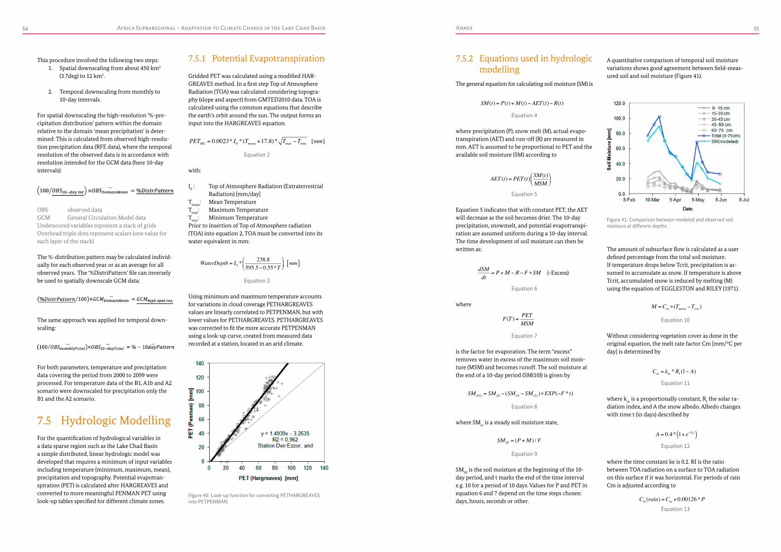
Africa Supraregional – Adaptation to Climate Change in the Lake Chad Basin54 55
A quantitative comparison of temporal soil moisture variations shows good agreement between field-meas-ured soil and soil moisture (Figure 41).
The amount of subsurface flow is calculated as a user defined percentage from the total soil moisture.If temperature drops below Tcrit, precipitation is as-sumed to accumulate as snow. If temperature is above Tcrit, accumulated snow is reduced by melting (M) using the equation of EGGLESTON and RILEY (1971).
Equation 10
Without considering vegetation cover as done in the original equation, the melt rate factor Cm [mm/°C per day] is determined by
Equation 11
where km is a proportionally constant, RI the solar ra-diation index, and A the snow albedo. Albedo changes with time t (in days) described by
Equation 12
where the time constant ke is 0.2. RI is the ratio between TOA radiation on a surface to TOA radiation on this surface if it was horizontal. For periods of rain Cm is adjusted according to
Equation 13
7.5.2 Equations used in hydrologic modelling
The general equation for calculating soil moisture (SM) is
Equation 4
where precipitation (P), snow melt (M), actual evapo-transpiration (AET) and run-off (R) are measured in mm. AET is assumed to be proportional to PET and the available soil moisture (SM) according to
Equation 5
Equation 5 indicates that with constant PET, the AET will decrease as the soil becomes drier. The 10-day precipitation, snowmelt, and potential evapotranspi-ration are assumed uniform during a 10-day interval. The time development of soil moisture can then be written as:
Equation 6
where
Equation 7
is the factor for evaporation. The term “excess” removes water in excess of the maximum soil mois-ture (MSM) and becomes runoff. The soil moisture at the end of a 10-day period (SM(10)) is given by
Equation 8
where SMss is a steady soil moisture state,
Equation 9
SM(0) is the soil moisture at the beginning of the 10-day period, and t marks the end of the time interval e.g. 10 for a period of 10 days. Values for P and PET in equation 6 and 7 depend on the time steps chosen: days, hours, seconds or other.
Annex
7.5.1 Potential Evapotranspiration
Gridded PET was calculated using a modified HAR-GREAVES method. In a first step Top of Atmosphere Radiation (TOA) was calculated considering topogra-phy (slope and aspect) from GMTED2010 data. TOA is calculated using the common equations that describe the earth’s orbit around the sun. The output forms an input into the HARGREAVES equation.
Equation 2
with:
I0 : Top of Atmosphere Radiation (Extraterrestrial Radiation) [mm/day]
Tmean: Mean TemperatureTmax: Maximum TemperatureTmin: Minimum TemperaturePrior to insertion of Top of Atmosphere radiation (TOA) into equation 2, TOA must be converted into its water equivalent in mm:
Equation 3
Using minimum and maximum temperature accounts for variations in cloud coverage PETHARGREAVES values are linearly correlated to PETPENMAN, but with lower values for PETHARGREAVES. PETHARGREAVES was corrected to fit the more accurate PETPENMAN using a look-up curve, created from measured data recorded at a station, located in an arid climate.
This procedure involved the following two steps:1. Spatial downscaling from about 450 km2
(3.7deg) to 12 km2.
2. Temporal downscaling from monthly to 10-day intervals.
For spatial downscaling the high-resolution ‘%-pre-cipitation distribution’ pattern within the domain relative to the domain ‘mean precipitation’ is deter-mined: This is calculated from observed high-resolu-tion precipitation data (RFE data), where the temporal resolution of the observed data is in accordance with resolution intended for the GCM data (here 10-day intervals):
OBS observed dataGCM General Circulation Model dataUnderscored variables represent a stack of gridsOverhead triple dots represent scalars (one value for each layer of the stack)
The %-distribution pattern may be calculated individ-ually for each observed year or as an average for all observed years. The ‘%DistriPattern’ file can inversely be used to spatially downscale GCM data:
The same approach was applied for temporal down-scaling:
For both parameters, temperature and precipitation data covering the period from 2000 to 2099 were processed. For temperature data of the B1, A1b and A2 scenario were downscaled for precipitation only the B1 and the A2 scenario.
7.5 Hydrologic ModellingFor the quantification of hydrological variables in a data sparse region such as the Lake Chad Basin a simple distributed, linear hydrologic model was developed that requires a minimum of input variables including temperature (minimum, maximum, mean), precipitation and topography. Potential evapotran-spiration (PET) is calculated after HARGREAVES and converted to more meaningful PENMAN PET using look-up tables specified for different climate zones.
PETHG = 0.0023* I0 *(Tmean +17.8)* Tmax −Tmin [mm]
WaterDepth = I0 *238.8
595.5− 0.55*T⎛
⎝⎜
⎞
⎠⎟ mm[ ]
Figure 40: Look-up function for converting PETHARGREAVES into PETPENMAN.
SM (t) = P(t)+M (t)− AET (t)− R(t)
AET (t) = PET (t) SM (t)MSM
⎛
⎝⎜
⎞
⎠⎟
dSMdt
= P +M − R−F ∗SM (-Excess)
F(T ) = PETMSM
SM (10) = SMSS − (SMSS − SM (0) )∗EXP(−F * t)
SMSS = (P +M ) / F
Figure 41: Comparison between modeled and observed soil moisture at different depths.
M =Cm ∗ (Tmean −Tcrit )
Cm = km *RI (1− A)
A = 0.4* 1+ e−ket( )
Cm (rain) =Cm + 0.00126*P

Africa Supraregional – Adaptation to Climate Change in the Lake Chad Basin56 57
The calculated magnitudes and phases are the inputs for measuring shape similarity. By excluding the higher magnitudes and phases from the similarity calculation, the influence of high-frequent noise is eliminated from the shape identification process. The objective is to eliminate most of the noise, however to preserve the diagnostic phenological features (Figure 42).
Through a Fourier transform and the elimination of the higher harmonics, a reduction of parameters is achieved which facilitates similarity measures. After the conversion from temporal space (x/y-data or rather time/NDVI-data) to Fourier space (magnitude and phase), the number of variables is reduced from 46 (for 16-day interval MODIS NDVI) to a total number of ten, if using the first five harmonics (Figure 43) or even six if just using the first three harmonics.
Following selection of a set of reference cycles, the algorithm searches for pixels with matching Fourier variables (magnitude and phase values). The challenge in shape classification is not so much to identify matching shapes but rather to allow for reasonable deviations from a perfect match due to natural shape variability and data noise. For this purpose, a set of controls is available to define individual accuracy thresholds.
Annex
and the phases as
Equation 22
F(Magnitude)u = Fourier magnitude FC(u) = Cosine (real part) FS(u) = Sine (imaginary part) F(Phase)u = Phase N = Number of samples / 2 f(x) = is the xth sample value
(here: xth NDVI value)u = Number of Fourier component
or harmonicx = Layer number or Julian Day of
NDVI layer (equal intervals)T = Length of time period covered;
where time is measured in number of NDVI-layers
Equation 17
where h is the head gradient given by terrain slope and l is flow distance given by pixel size and flow direction. Total travel times from each pixel to the pour point are calculated as described for the surface flow.
7.6 Classification of Vegetation Cycles (Ecosystems)
Biomass classifications of the Chad Basin and of the Yaere-Naga wetlands were implemented using an algorithm developed by authors of this study. Some of its advantages include (i) a subtle distinction of vegetation cycles of different shapes, (ii) the inter-pretation of vegetation covers based on their seasonal biomass variation (not just a single point in time), and (iii) the classifications’ spatial and temporal compar-ability, required for change detection.
A major element of the classification is the conversion of NDVI time series from temporal space to Fourier space using a Discrete Fourier Transform (DFT). Using a DFT, the shape of a complex, and periodic cycle like an NDVI cycle can be decomposed into its individual frequencies, where each frequency is described by its individual magnitude and phase. The DFT is written as
Equation 18
which can be decomposed into a real part (Eq.19) and an imaginary part (Eq.20)
Equation 19
Equation 20
with the magnitudes calculated as
Equation 21
where P is precipitation (mm).In addition to the excess water (Equation 3), the amount of precipitation that becomes runoff (R) is triggered by slope according to:
Equation 14
Values for CRO range between 0.08 and 0.35 and depend on slope ranges as defined in Caltran’s Storm Water Quality Handbook (2003).
To calculate the time it takes surface run-off to reach a defined pour point we used the equations from Man-ning for sheet flow:
Equation 15
whereTt = travel time [hr]N = Manning’s roughness coefficientL = flow length [ft]P2 = 2-year, 24-hour rainfall [in]s = slope of hydraulic grade line [ft/ft]and for open channel flow
Equation 16
whereV = VelocityK = 1 when measured in meters and seconds, 1.49 for
feet and secondsS = channel slopen = Manning coefficient; differs for different materials A= Area of channel [ft2]P = Perimeter of channel [ft] (wetted perimeter)A/P = also called hydraulic radius Rh
Knowing pixel size and flow direction, the calculated velocities can be converted to travel times. The crite-rion for open channel is a minimum number of pixels that flow into a pixel, which is defined by the user.
Travel time is calculated for each pixel. Total travel time from a specific location is the sum of travel-times along the flow path from that pixel to the pour point. The calculation of subsurface flow velocities VF in a porous medium of a distinct transmissivity k follows Darcy
R =CRO ∗P
Tt =0.007(n*L)0.8
P2( )0.5 s0.4
V =knAP⎛
⎝⎜
⎞
⎠⎟2/3
S1/2
VF = khl
F(u) =1N x=0
N−1
Σ fx × e−2πux /T
FC(u) =1N
f (x)× cos 2π uxT
⎛
⎝⎜
⎞
⎠⎟
⎛
⎝⎜
⎞
⎠⎟
x=0
N−1
∑
FS(u) =1N
f (x)× sin 2π uxT
⎛
⎝⎜
⎞
⎠⎟
⎛
⎝⎜
⎞
⎠⎟
x=0
N−1
∑
F(Magnitude)u = FC(u)2 +F S(u)
2
F(Phase)u = tanFC(u)FS(u)
⎛
⎝⎜⎜
⎞
⎠⎟⎟
Figure 42: Fourier filtered biomass cycle (red curve; created through inverse Fourier transform) after removing noise (blue curve) from the original biomass cycle (green curve) using a discrete Fourier transform function37.
Figure 43: Magnitudes (left) and phases (right) of a biomass cycle as shown in Figure 42.
37 From the original 11 harmonics in the original cycle only har-monics 1 to 5 are preserved in the Fourier filtered cycle. The 23 intervals along the x-axis represent one year. The biomass cycle is double peaked, representing a double-cropped area.
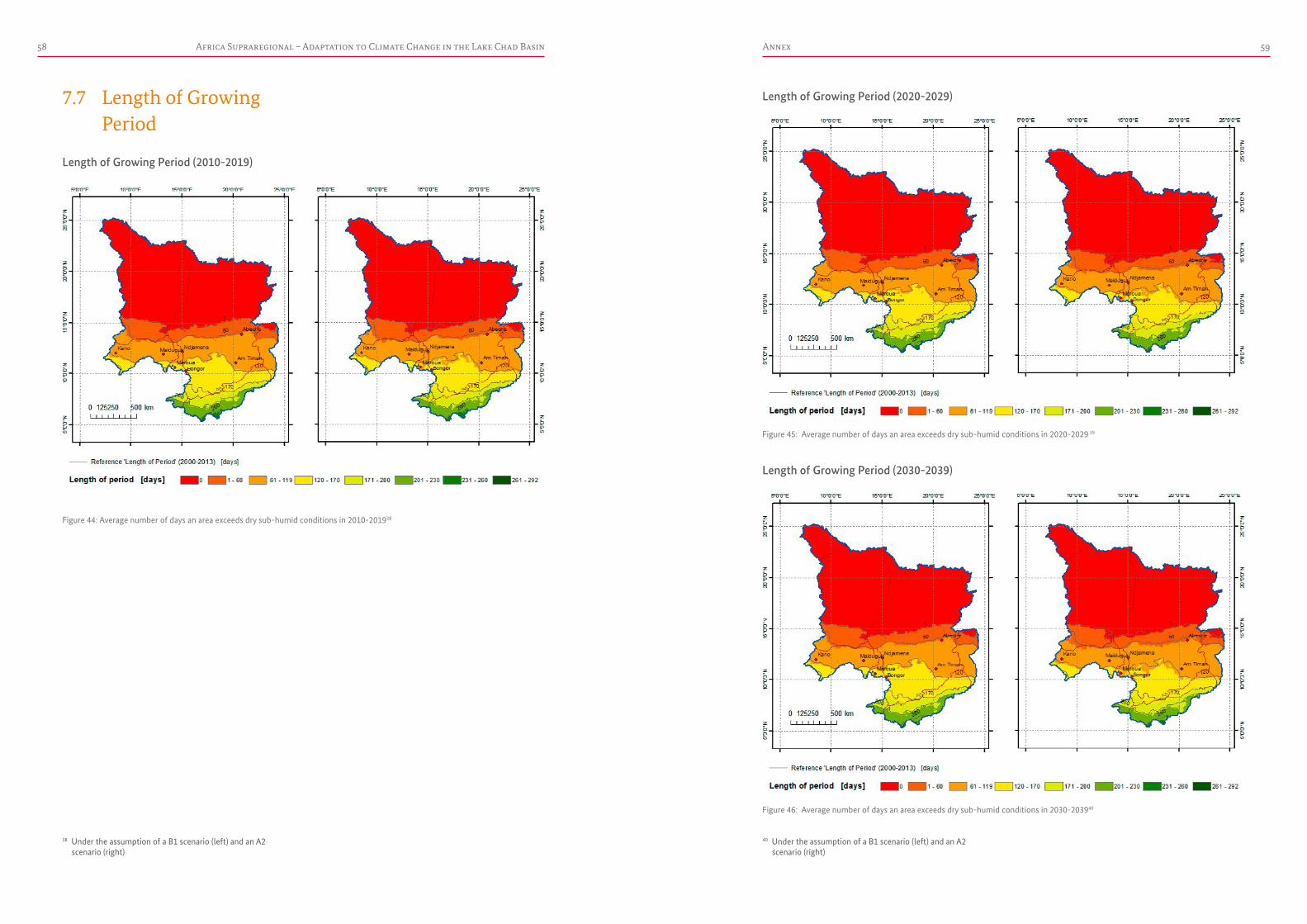
Africa Supraregional – Adaptation to Climate Change in the Lake Chad Basin58 59Annex
7.7 Length of Growing Period
Length of Growing Period (2010-2019)
Length of Growing Period (2020-2029)
Length of Growing Period (2030-2039)
Figure 44: Average number of days an area exceeds dry sub-humid conditions in 2010-201938
Figure 45: Average number of days an area exceeds dry sub-humid conditions in 2020-2029 39
Figure 46: Average number of days an area exceeds dry sub-humid conditions in 2030-203940
38 Under the assumption of a B1 scenario (left) and an A2 scenario (right)
40 Under the assumption of a B1 scenario (left) and an A2 scenario (right)
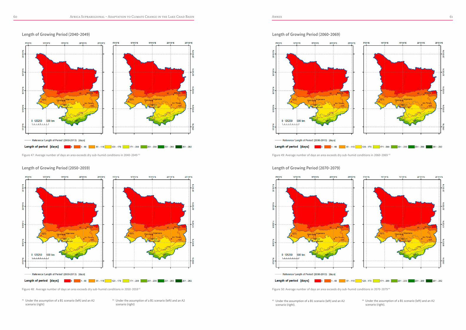
Africa Supraregional – Adaptation to Climate Change in the Lake Chad Basin60 61Annex
Length of Growing Period (2040-2049) Length of Growing Period (2060-2069)
Figure 47: Average number of days an area exceeds dry sub-humid conditions in 2040-2049 41 Figure 49: Average number of days an area exceeds dry sub-humid conditions in 2060-2069 43
41 Under the assumption of a B1 scenario (left) and an A2 scenario (right)
43 Under the assumption of a B1 scenario (left) and an A2 scenario (right).
44 Under the assumption of a B1 scenario (left) and an A2 scenario (right).
42 Under the assumption of a B1 scenario (left) and an A2 scenario (right)
Length of Growing Period (2050-2059) Length of Growing Period (2070-2079)
Figure 48: Average number of days an area exceeds dry sub-humid conditions in 2050-2059 42 Figure 50: Average number of days an area exceeds dry sub-humid conditions in 2070-2079 44

Africa Supraregional – Adaptation to Climate Change in the Lake Chad Basin62 63Annex
Length of Growing Period (2080-2089)
Figure 51: Average number of days an area exceeds dry sub-humid conditions in 2080-2089 45
45 Under the assumption of a B1 scenario (left) and an A2 scenario (right)
46 Under the assumption of a B1 scenario (left) and an A2 scenario (right)
Length of Growing Period (2090-2099)
Figure 52: Average number of days an area exceeds dry sub-humid conditions in 2090-2099 46
Figure 53: PET Increase by 2010-2019 for a B1 (left) and an A2 Scenario (right)
Figure 54: PET Increase by 2020-2029 for a B1 (left) and an A2 Scenario (right)
7.8 PET Increase
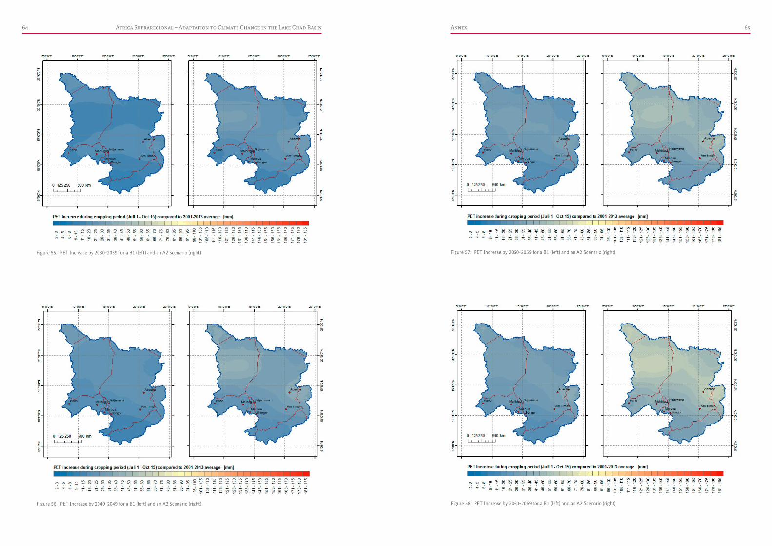
Africa Supraregional – Adaptation to Climate Change in the Lake Chad Basin64 65Annex
Figure 55: PET Increase by 2030-2039 for a B1 (left) and an A2 Scenario (right) Figure 57: PET Increase by 2050-2059 for a B1 (left) and an A2 Scenario (right)
Figure 56: PET Increase by 2040-2049 for a B1 (left) and an A2 Scenario (right) Figure 58: PET Increase by 2060-2069 for a B1 (left) and an A2 Scenario (right)
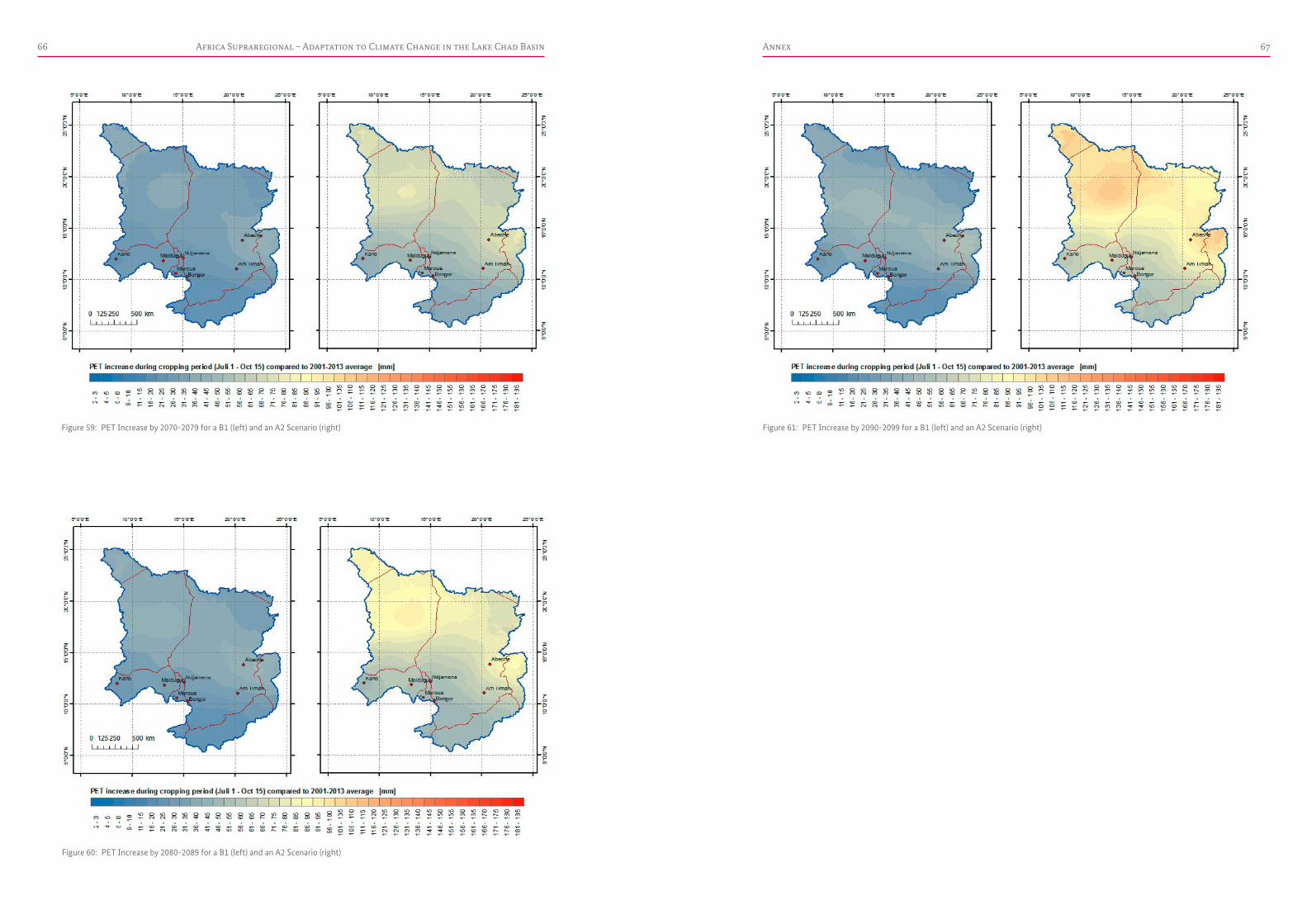
Africa Supraregional – Adaptation to Climate Change in the Lake Chad Basin66 67Annex
Figure 59: PET Increase by 2070-2079 for a B1 (left) and an A2 Scenario (right) Figure 61: PET Increase by 2090-2099 for a B1 (left) and an A2 Scenario (right)
Figure 60: PET Increase by 2080-2089 for a B1 (left) and an A2 Scenario (right)
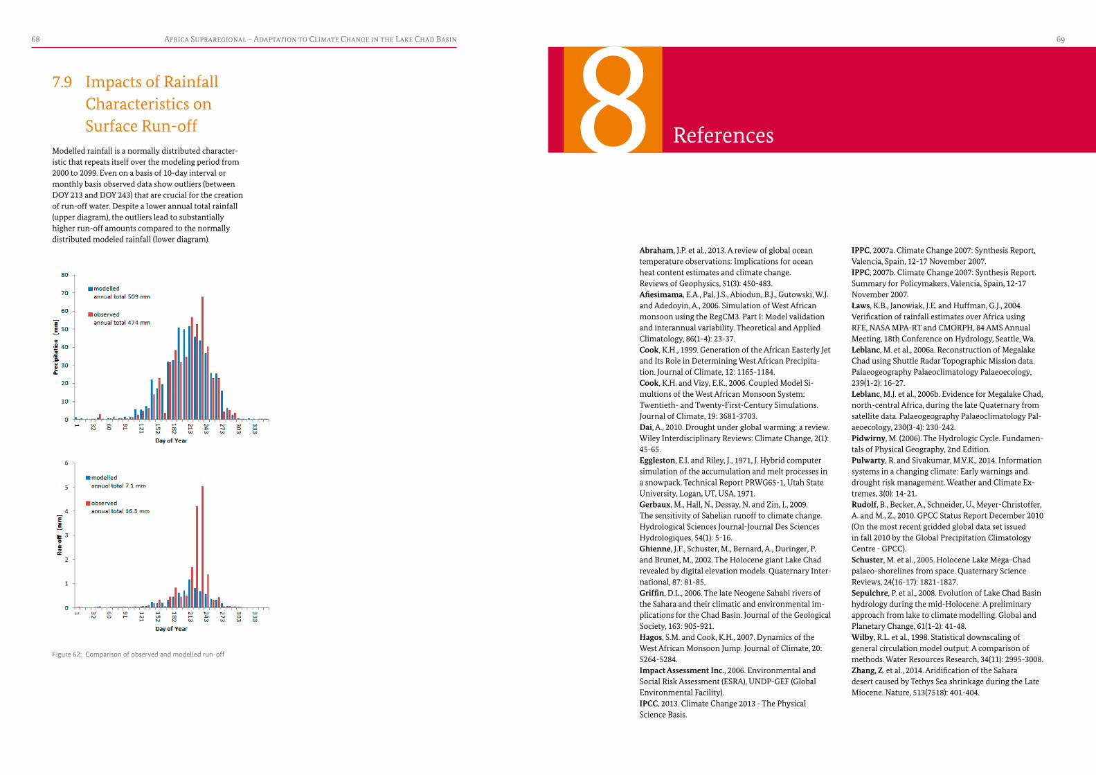
Africa Supraregional – Adaptation to Climate Change in the Lake Chad Basin68 69
IPPC, 2007a. Climate Change 2007: Synthesis Report, Valencia, Spain, 12-17 November 2007.IPPC, 2007b. Climate Change 2007: Synthesis Report. Summary for Policymakers, Valencia, Spain, 12-17 November 2007.Laws, K.B., Janowiak, J.E. and Huffman, G.J., 2004. Verification of rainfall estimates over Africa using RFE, NASA MPA-RT and CMORPH, 84 AMS Annual Meeting, 18th Conference on Hydrology, Seattle, Wa.Leblanc, M. et al., 2006a. Reconstruction of Megalake Chad using Shuttle Radar Topographic Mission data. Palaeogeography Palaeoclimatology Palaeoecology, 239(1-2): 16-27.Leblanc, M.J. et al., 2006b. Evidence for Megalake Chad, north-central Africa, during the late Quaternary from satellite data. Palaeogeography Palaeoclimatology Pal-aeoecology, 230(3-4): 230-242.Pidwirny, M. (2006). The Hydrologic Cycle. Fundamen-tals of Physical Geography, 2nd Edition.Pulwarty, R. and Sivakumar, M.V.K., 2014. Information systems in a changing climate: Early warnings and drought risk management. Weather and Climate Ex-tremes, 3(0): 14-21.Rudolf, B., Becker, A., Schneider, U., Meyer-Christoffer, A. and M., Z., 2010. GPCC Status Report December 2010 (On the most recent gridded global data set issued in fall 2010 by the Global Precipitation Climatology Centre - GPCC).Schuster, M. et al., 2005. Holocene Lake Mega-Chad palaeo-shorelines from space. Quaternary Science Reviews, 24(16-17): 1821-1827.Sepulchre, P. et al., 2008. Evolution of Lake Chad Basin hydrology during the mid-Holocene: A preliminary approach from lake to climate modelling. Global and Planetary Change, 61(1-2): 41-48.Wilby, R.L. et al., 1998. Statistical downscaling of general circulation model output: A comparison of methods. Water Resources Research, 34(11): 2995-3008.Zhang, Z. et al., 2014. Aridification of the Sahara desert caused by Tethys Sea shrinkage during the Late Miocene. Nature, 513(7518): 401-404.
Abraham, J.P. et al., 2013. A review of global oceantemperature observations: Implications for ocean heat content estimates and climate change. Reviews of Geophysics, 51(3): 450-483.Afiesimama, E.A., Pal, J.S., Abiodun, B.J., Gutowski, W.J. and Adedoyin, A., 2006. Simulation of West African monsoon using the RegCM3. Part I: Model validation and interannual variability. Theoretical and Applied Climatology, 86(1-4): 23-37.Cook, K.H., 1999. Generation of the African Easterly Jetand Its Role in Determining West African Precipita-tion. Journal of Climate, 12: 1165-1184.Cook, K.H. and Vizy, E.K., 2006. Coupled Model Si-multions of the West African Monsoon System: Twentieth- and Twenty-First-Century Simulations. Journal of Climate, 19: 3681-3703.Dai, A., 2010. Drought under global warming: a review. Wiley Interdisciplinary Reviews: Climate Change, 2(1): 45-65.Eggleston, E.I. and Riley, J., 1971, J. Hybrid computer simulation of the accumulation and melt processes in a snowpack. Technical Report PRWG65-1, Utah State University, Logan, UT, USA, 1971.Gerbaux, M., Hall, N., Dessay, N. and Zin, I., 2009. The sensitivity of Sahelian runoff to climate change. Hydrological Sciences Journal-Journal Des Sciences Hydrologiques, 54(1): 5-16.Ghienne, J.F., Schuster, M., Bernard, A., Duringer, P. and Brunet, M., 2002. The Holocene giant Lake Chad revealed by digital elevation models. Quaternary Inter-national, 87: 81-85.Griffin, D.L., 2006. The late Neogene Sahabi rivers of the Sahara and their climatic and environmental im-plications for the Chad Basin. Journal of the Geological Society, 163: 905-921.Hagos, S.M. and Cook, K.H., 2007. Dynamics of the West African Monsoon Jump. Journal of Climate, 20: 5264-5284.Impact Assessment Inc., 2006. Environmental and Social Risk Assessment (ESRA), UNDP-GEF (Global Environmental Facility).IPCC, 2013. Climate Change 2013 - The Physical Science Basis.
7.9 Impacts of Rainfall Characteristics on Surface Run-off
Modelled rainfall is a normally distributed character-istic that repeats itself over the modeling period from 2000 to 2099. Even on a basis of 10-day interval or monthly basis observed data show outliers (between DOY 213 and DOY 243) that are crucial for the creation of run-off water. Despite a lower annual total rainfall (upper diagram), the outliers lead to substantially higher run-off amounts compared to the normally distributed modeled rainfall (lower diagram).
Figure 62: Comparison of observed and modelled run-off
References8


Published by Deutsche Gesellschaft für Internationale Zusammenarbeit (GIZ) GmbH
Registered offices Bonn and Eschborn, Germany
Programme „Sustainable Water Resources Management“ Project „Adaptation to Climate Change in the Lake Chad Basin“Godesberger Allee 119 53175 Bonn Germany Tel. +49 (0) 228 44 60 - 0 Fax +49 (0) 228 44 60 - 1766
Dag-Hammarskjöld-Weg 1-5 65760 Eschborn Germany Tel. +49 (0) 6196 79 - 0 Fax +49 (0) 6196 79 - 1115
[email protected] www.giz.de
Edited by AHT GROUP AG
Design and Layout Diamond media GmbH, Neunkirchen-Seelscheid
Printed by f & m Satz & Druckerei GmbH & Co. KG Eifelstr. 2 -4 53757 Sankt Augustin
Photo credits Helmut Kulitz , Dr. Gabriele Lames
As at February 2015 GIZ is responsible for the content of this publication.
On behalf of Federal Ministry for Economic Cooperation and Development (BMZ)
Adresses of the BMZ officesBMZ Bonn Dahlmannstraße 4 53113 Bonn Germany Tel. +49 (0) 228 99 535 - 0 Fax +49 (0) 228 99 535 - 3500 BMZ Berlin
Stresemannstraße 94 10963 Berlin Germany Tel. +49 (0) 30 18 535 - 0 Fax +49 (0) 30 18 535 - 2501 [email protected] www.bmz.de
Imprint