afrl-rh-fs-tr-2019-0005 the ability of a color appearance
TRANSCRIPT
AFRL-RH-FS-TR-2019-0005
The Ability of a Color Appearance Model to Predict the Appearance of Colors Viewed
Through Laser Eye Protection Filters James R. Dykes Thomas K. Kuyk
Rachel J. Singleton Paul V. Garcia Peter A. Smith
SAIC
Brenda J. Novar Leon N. McLin Barry P. Goettl
711th Human Performance Wing Airman Systems Directorate
Bioeffects Division Optical Radiation Bioeffects Branch
July 2018 Interim Report for Sep 1, 2010 – July 30, 2018
DESTRUCTION NOTICE – Destroy by any method that will prevent disclosure of contents or reconstruction of this document.
Air Force Research Laboratory 711th Human Performance Wing Airman Systems Directorate Bioeffects Division Optical Radiation Bioeffects Branch JBSA Fort Sam Houston, Texas 78234
Distribution Statement A. Approved for public release; distribution is unlimited. TSRL-PA-2019-0149. The opinions expressed on this document, electronic or otherwise, are solely those of the author(s). They do not represent an endorsement by or the views of the United States Air Force, the Department of Defense, or the United States Government.
NOTICE AND SIGNATURE PAGE
Using Government drawings, specifications, or other data included in this document for any purpose other than Government procurement does not in any way obligate the U.S. Government. The fact that the Government formulated or supplied the drawings, specifications, or other data does not license the holder or any other person or corporation; or convey any rights or permission to manufacture, use, or sell any patented invention that may relate to them.
This report was cleared for public release by the 88th ABW Public Affairs Office and is available to the general public, including foreign nationals. Copies may be obtained from the Defense Technical Information Center (DTIC) (http://www.dtic.mil).
(AFRL-RH-FS-TR- ) has been reviewed and is approved for publication inaccordance with assigned distribution statement.
_______________________________________
_______________________________________
"The Ability of a Color Appearance Model to Predict the Appearance of Colors Viewed through Laser Eye Protection Filters"
2019 - 0005
Digitally signed by SHORTER.PATRICK.D.1023156390 Date: 2019.04.10 11:13:33 -05'00'
MILLER.STEPHANIE.A.1230536283
Digitally signed by MILLER.STEPHANIE.A.1230536283Date: 2019.04.10 16:20:50 -05'00'
PATRICK SHORTER, Maj., USAF Branch Chief Optical Radiation Bioeffects Branch
REPORT DOCUMENTATION PAGE Form Approved OMB No. 0704-0188
Public reporting burden for this collection of information is estimated to average 1 hour per response, including the time for reviewing instructions, searching existing data sources, gathering and maintaining the data needed, and completing and reviewing this collection of information. Send comments regarding this burden estimate or any other aspect of this collection of information, including suggestions for reducing this burden to Department of Defense, Washington Headquarters Services, Directorate for Information Operations and Reports (0704-0188), 1215 Jefferson Davis Highway, Suite 1204, Arlington, VA 22202-4302. Respondents should be aware that notwithstanding any other provision of law, no person shall be subject to any penalty for failing to comply with a collection of information if it does not display a currently valid OMB control number. PLEASE DO NOT RETURN YOUR FORM TO THE ABOVE ADDRESS. 1. REPORT DATE (DD-MMYYYY) 01-07-2018
2. REPORT TYPEInterim Technical Report
3. DATES COVERED (From - To) Sep 1, 2010 – July 30, 2018
4. TITLE AND SUBTITLE
The Ability of a Color Appearance Model to Predict the Appearance of Colors Viewed through Laser Eye Protection Filters
5a. CONTRACT NUMBER FA8650-14-D-6519 5b. GRANT NUMBER
5c. PROGRAM ELEMENT NUMBER
6. AUTHOR(S)
Dykes, James R, Kuyk, Thomas K., Singleton, Rachel J, Garcia, Paul V., Smith, Peter A., Novar, Brenda J., McLin, Leon N., and Goettl, Barry, P.
5d. PROJECT NUMBER
5e. TASK NUMBER
5f. WORK UNIT NUMBER H0NB
7. PERFORMING ORGANIZATION NAME(S) AND ADDRESS(ES)Air Force Research Laboratory SAIC
8. PERFORMING ORGANIZATION REPORT NUMBER
711th Human Performance Wing 4141 Petroleum Rd Airman Systems Directorate Fort Sam Houston Bioeffects Division TX 78234-2644 Optical Radiation Bioeffects Branch 9. SPONSORING / MONITORING AGENCY NAME(S) AND ADDRESS(ES) 10. SPONSOR/MONITOR’S ACRONYM(S)Air Force Research Laboratory711th Human Performance Wing Airman Systems Directorate Bioeffects Division Optical Radiation Bioeffects Branch JBSA Fort Sam Houston, TX 78234-2644
711 HPW/RHDO
11. SPONSOR/MONITOR’S REPORTNUMBER(S)
AFRL-RH-FS-TR-2019-0005 12. DISTRIBUTION / AVAILABILITY STATEMENTDistribution A. Approved for public release; distribution is unlimited. TSRL-PA-2019-0149. The opinions expressed on this document, electronic or otherwise, are solely those of the author(s). They do not represent an endorsement by or the views of the United States Air Force, the Department of Defense, or the United StatesGovernment. 13. SUPPLEMENTARY NOTES
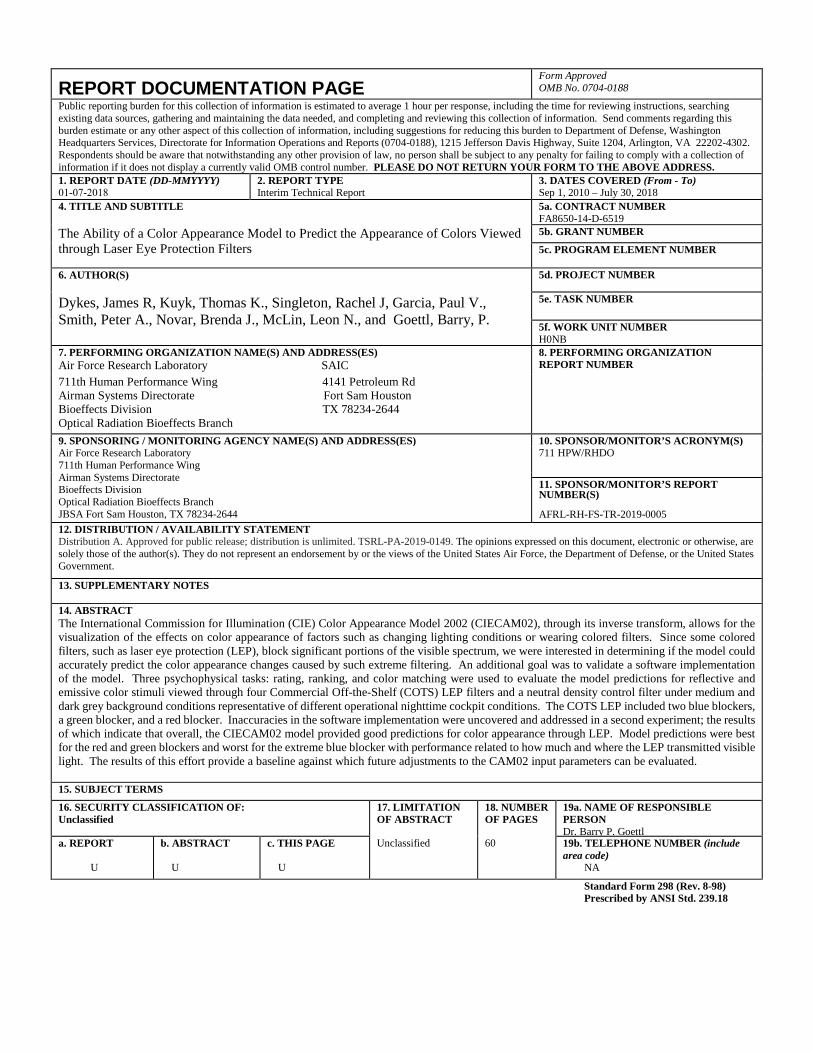
14. ABSTRACTThe International Commission for Illumination (CIE) Color Appearance Model 2002 (CIECAM02), through its inverse transform, allows for thevisualization of the effects on color appearance of factors such as changing lighting conditions or wearing colored filters. Since some coloredfilters, such as laser eye protection (LEP), block significant portions of the visible spectrum, we were interested in determining if the model couldaccurately predict the color appearance changes caused by such extreme filtering. An additional goal was to validate a software implementationof the model. Three psychophysical tasks: rating, ranking, and color matching were used to evaluate the model predictions for reflective andemissive color stimuli viewed through four Commercial Off-the-Shelf (COTS) LEP filters and a neutral density control filter under medium anddark grey background conditions representative of different operational nighttime cockpit conditions. The COTS LEP included two blue blockers, a green blocker, and a red blocker. Inaccuracies in the software implementation were uncovered and addressed in a second experiment; the results of which indicate that overall, the CIECAM02 model provided good predictions for color appearance through LEP. Model predictions were bestfor the red and green blockers and worst for the extreme blue blocker with performance related to how much and where the LEP transmitted visible light. The results of this effort provide a baseline against which future adjustments to the CAM02 input parameters can be evaluated.
15. SUBJECT TERMS 16. SECURITY CLASSIFICATION OF: Unclassified
17. LIMITATION OF ABSTRACT
18. NUMBER OF PAGES
19a. NAME OF RESPONSIBLE PERSON Dr. Barry P. Goettl
a. REPORT
U
b. ABSTRACT
U
c. THIS PAGE
U
Unclassified 60 19b. TELEPHONE NUMBER (include area code)
NA
Standard Form 298 (Rev. 8-98) Prescribed by ANSI Std. 239.18
This Page Intentionally Left Blank
i
Distribution A. Approved for public release; distribution is unlimited. TSRL-PA-2019-0149. The opinions expressed on this document, electronic of otherwise, are solely those of the author(s). They do not represent an endorsement by or the views of the
United State Air Force, the Department of Defense, or the United States Government.
TABLE OF CONTENTS Section Page TABLE OF CONTENTS ................................................................................................................. i
LIST OF FIGURES ....................................................................................................................... iii
LIST OF TABLES .......................................................................................................................... v
1 BACKGROUND .................................................................................................................... 1
2 METHODS ............................................................................................................................. 4
2.1 Overview of Experiment and Design ............................................................................... 4
2.2 Filters ................................................................................................................................ 4
2.3 Lanthony 40 Hue Test ...................................................................................................... 6
2.4 Display Parameters ........................................................................................................... 7
2.5 Stimuli .............................................................................................................................. 8
2.6 Ranking, Rating and Color Matching Tasks .................................................................... 9
2.7 CIECAM02 Implementation ............................................................................................ 9
2.8 Subjects .......................................................................................................................... 10
2.9 Experimental Design ...................................................................................................... 11
2.9.1 Experiment 1 ........................................................................................................... 11
2.9.2 Experiment 2 ........................................................................................................... 11
3 Results ................................................................................................................................... 12
3.1 Experiment 1 .................................................................................................................. 12
3.1.1 Lanthony 40 ............................................................................................................ 12
3.1.2 Ranking ................................................................................................................... 15
3.1.3 Rating ...................................................................................................................... 16
3.1.4 Color Matching ....................................................................................................... 17
3.1.5 Issues with Experiment 1 ........................................................................................ 21
3.2 Experiment 2 .................................................................................................................. 22
3.2.1 Ranking ................................................................................................................... 22
3.2.2 Rating ...................................................................................................................... 23
3.2.3 Color Matching ....................................................................................................... 25
4 CONCLUSIONS................................................................................................................... 32
ii
Distribution A. Approved for public release; distribution is unlimited. TSRL-PA-2019-0149. The opinions expressed on this document, electronic of otherwise, are solely those of the author(s). They do not represent an endorsement by or the views of the
United State Air Force, the Department of Defense, or the United States Government.
REFERENCES ............................................................................................................................. 36
APPENDIX A - Experiment 1: Graphs for All Filters .............................................................. A-1
APPENDIX B - Experiment 2: Graphs for All Filters .............................................................. B-1
iii
Distribution A. Approved for public release; distribution is unlimited. TSRL-PA-2019-0149. The opinions expressed on this document, electronic of otherwise, are solely those of the author(s). They do not represent an endorsement by or the views of the
United State Air Force, the Department of Defense, or the United States Government.
LIST OF FIGURES Figure 1. Transmission spectra of COTS filters plotted against output of the R, G, and B
monitor channels (top panel) and relative sensitivity of the L-, M-, and S-cones (bottom panel) .................................................................................................................5
Figure 2. ND40% and COTS filters (reflective lab coat above labels and emissive monitor below labels) ....................................................................................................................6
Figure 3. Lanthony 40 Hue Test .....................................................................................................7
Figure 4. Haploscopic viewing setup with CS-200 ........................................................................8
Figure 5. Luminance output (Y) of the red, green, and blue (RGB) channels of the monitor and the white stimulus over an approximate seven-month period ..................................8
Figure 6. Mean Score index (SI) for Lanthony 40 hue test for each filter. Error bars ± 1 SE. *** p< .001 .......................................................................................................12
Figure 7. Mean errors/cap for Lanthony 40 hue test for each filter ..............................................13
Figure 8. Lanthony 40 Caps with high SI scores (top left panel) and Lanthony 40 caps relative to monitor display gamut (triangle in top right panel). The middle left and right panels show the translation effects of the RBlkr and GBlkr filters. The bottom panels show the linear compression along the red/ green axis for the blue blockers (BBlkr1 & BBlkr2) .........................................................................................14
Figure 9. The top left and right panels show that adaptation reduces the translation effects of the RBlkr and GBlkr filters. The bottom panels show that adaptation reduces the translation effects of the blue blockers (BBlkr1 & BBlkr2), but did not reduce the linear compression along the red/ green axis for BBlkr2 ........................................15
Figure 10. Winsorized mean rankings for the predictions with each filter ...................................16
Figure 11. Scatterplots relating rankings and ratings in Experiment 1 .........................................17
Figure 12. The effects of stimulus color and background (medium or dark) on d E*uv (top panels), d L* (middle panels), and d u*v* (bottom panels) for the RBlkr filter (left panels) and the BBlkr1 filter (right panels). Error bars ± 1 SE ............................19
Figure 13. The effects of the RBlkr and BBlkr1 filters and adaptation. The diamonds are the nine unfiltered stimuli. The tail of the arrows are the filtered stimuli and the tip of the arrows are filtered and adapted predictions ...................................................20
Figure 14. Subject matches relative to filtered and adapted predictions (arrow tips) for RBlkr and BBlkr1 filters. Squares are matches with the dark grey background and circles are matches with the medium grey background ..........................................21
Figure 15. Winsorized mean rankings for the predictions with each filter in Experiment 2 ........23
Figure 16. Scatterplots relating rankings and ratings in Experiment 2 .........................................24
iv
Distribution A. Approved for public release; distribution is unlimited. TSRL-PA-2019-0149. The opinions expressed on this document, electronic of otherwise, are solely those of the author(s). They do not represent an endorsement by or the views of the
United State Air Force, the Department of Defense, or the United States Government.
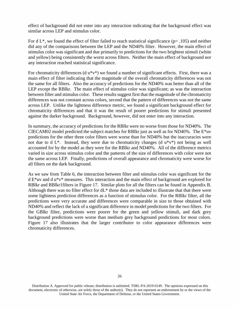
Figure 17. The effects of stimulus color and background (medium or dark) on d E*uv (top panel), d L* (middle panel), and d u*v* (bottom panel) for the RBlkr and BBlkr1 filters. Error bars ± 1 SE ...............................................................................................27
Figure 18. The effects of each filter and adaptation. The diamonds are the nine unfiltered stimuli. The tail of the arrows are the filtered stimuli and the tip of the arrows are filtered and adapted predictions ...............................................................................28
Figure 19. Subject matches relative to filtered and adapted predictions (arrow tips). Squares are matches with the dark grey background and circles are matches with the medium grey background ........................................................................................28
Figure 20. The effect of CIECAM02 adaptation on E94 differences for each stimulus color with each filter ...............................................................................................................30
v
Distribution A. Approved for public release; distribution is unlimited. TSRL-PA-2019-0149. The opinions expressed on this document, electronic of otherwise, are solely those of the author(s). They do not represent an endorsement by or the views of the
United State Air Force, the Department of Defense, or the United States Government.
LIST OF TABLES Table 1. Primary CIECAM02 Parameters ....................................................................................10
Table 2. Proportion of variance accounted for (r²) between the ratings and rankings of the predictions in Experiment 1 ..........................................................................................16
Table 3. Results of the test for differences between filters ...........................................................18
Table 4. Euclidean u’v’ matching errors that produce ratings in the “Unacceptable” range (1- 3.5) and in the “Acceptable” range (3.5- 6) .............................................................22
Table 5. Proportion of variance accounted for (r²) between the ratings and rankings of the predictions in Experiment 2 ..........................................................................................25
Table 6. Results of the ANOVA for the Matching Data in Experiment 2 ....................................25
Table 7. E94 differences averaged across the stimuli for each of the filters ................................29
Table 8. Euclidean u’v’ matching errors that produce ratings in the “Unacceptable” range (1- 3.5) and in the “Acceptable” range (3.5- 6) .............................................................31
vi
Distribution A. Approved for public release; distribution is unlimited. TSRL-PA-2019-0149. The opinions expressed on this document, electronic of otherwise, are solely those of the author(s). They do not represent an endorsement by or the views of the
United State Air Force, the Department of Defense, or the United States Government.
This Page Intentionally Left Blank
1
Distribution A. Approved for public release; distribution is unlimited. TSRL-PA-2019-0149. The opinions expressed on this document, electronic of otherwise, are solely those of the author(s). They do not represent an endorsement by or the views of the
United State Air Force, the Department of Defense, or the United States Government.
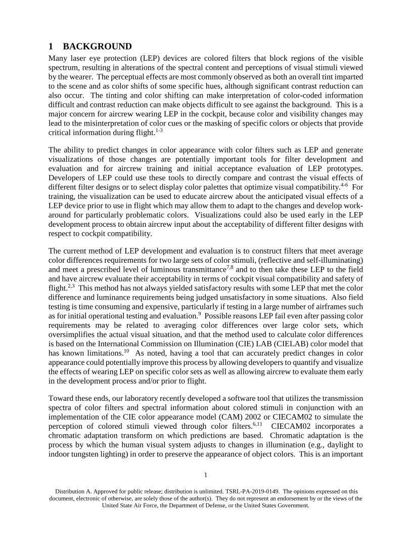
1 BACKGROUND Many laser eye protection (LEP) devices are colored filters that block regions of the visible spectrum, resulting in alterations of the spectral content and perceptions of visual stimuli viewed by the wearer. The perceptual effects are most commonly observed as both an overall tint imparted to the scene and as color shifts of some specific hues, although significant contrast reduction can also occur. The tinting and color shifting can make interpretation of color-coded information difficult and contrast reduction can make objects difficult to see against the background. This is a major concern for aircrew wearing LEP in the cockpit, because color and visibility changes may lead to the misinterpretation of color cues or the masking of specific colors or objects that provide critical information during flight.1-3
The ability to predict changes in color appearance with color filters such as LEP and generate visualizations of those changes are potentially important tools for filter development and evaluation and for aircrew training and initial acceptance evaluation of LEP prototypes. Developers of LEP could use these tools to directly compare and contrast the visual effects of different filter designs or to select display color palettes that optimize visual compatibility.4-6 For training, the visualization can be used to educate aircrew about the anticipated visual effects of a LEP device prior to use in flight which may allow them to adapt to the changes and develop work-around for particularly problematic colors. Visualizations could also be used early in the LEP development process to obtain aircrew input about the acceptability of different filter designs with respect to cockpit compatibility.
The current method of LEP development and evaluation is to construct filters that meet average color differences requirements for two large sets of color stimuli, (reflective and self-illuminating) and meet a prescribed level of luminous transmittance7,8 and to then take these LEP to the field and have aircrew evaluate their acceptability in terms of cockpit visual compatibility and safety of flight.2,3 This method has not always yielded satisfactory results with some LEP that met the color difference and luminance requirements being judged unsatisfactory in some situations. Also field testing is time consuming and expensive, particularly if testing in a large number of airframes such as for initial operational testing and evaluation.9 Possible reasons LEP fail even after passing color requirements may be related to averaging color differences over large color sets, which oversimplifies the actual visual situation, and that the method used to calculate color differences is based on the International Commission on Illumination (CIE) LAB (CIELAB) color model that has known limitations.10 As noted, having a tool that can accurately predict changes in color appearance could potentially improve this process by allowing developers to quantify and visualize the effects of wearing LEP on specific color sets as well as allowing aircrew to evaluate them early in the development process and/or prior to flight.
Toward these ends, our laboratory recently developed a software tool that utilizes the transmission spectra of color filters and spectral information about colored stimuli in conjunction with an implementation of the CIE color appearance model (CAM) 2002 or CIECAM02 to simulate the perception of colored stimuli viewed through color filters.6,11 CIECAM02 incorporates a chromatic adaptation transform on which predictions are based. Chromatic adaptation is the process by which the human visual system adjusts to changes in illumination (e.g., daylight to indoor tungsten lighting) in order to preserve the appearance of object colors. This is an important
2
Distribution A. Approved for public release; distribution is unlimited. TSRL-PA-2019-0149. The opinions expressed on this document, electronic of otherwise, are solely those of the author(s). They do not represent an endorsement by or the views of the
United State Air Force, the Department of Defense, or the United States Government.
factor to take into consideration regarding the design of LEP, primarily because much of the initial change in color appearance after first donning LEP rapidly diminishes due to chromatic adaptation.
Our simulation approach was similar to that taken by Lucassen4, but we incorporated a recent color appearance model.11 Lucassen implemented two models of chromatic adaptation to produce visualizations of LEP effects, the von Kries adaptation12 and a second model based on their empirical research.13 The von Kries model is a simple linear model that assumes each cone type adapts independently and maintains constant output during the adaptation process. In contrast, in the Lucassen and Walraven model the cone response functions are non-linear. As seen in their visualizations, the result of von Kries adaptation on colored stimuli viewed through LEP was nearly complete recovery of color appearance to the original, unfiltered state. In contrast, the Lucassen and Walraven model yielded results between a filtered, but unadapted state, and the original unfiltered state; in other words chromatic adaptation was not as complete. Since Lucassen’s demonstration, the CIE has adopted the newer and more powerful CIECAM02.11 At its core is a von Kries-type linear transformation, however in contrast to earlier CIE models like CIELAB it works on cone photoreceptor responses rather than CIE tristimulus values and it incorporates a number of other parameters that control the linearity of the output and degree of adaptation.10,14
As noted previously, for applications involving LEP, the United States Air Force (USAF) currently specifies color difference levels that LEP must meet. To do this, colors are specified in CIELAB space and the color difference between the unfiltered and filtered stimuli is calculated using the E94 color difference formula.8 Although this approach has been widely used for many decades, it has limitations. As a color appearance model, CIELAB incorporates what has been referred to as “the wrong von Kries chromatic adaptation transform” that operates on CIE tristimulus values rather than cone photoreceptor responses. As a result, it has deficiencies in predicting hue changes with changes in luminance. It also does not provide absolute correlates for appearance attributes of brightness and colorfulness and other color appearance phenomena that are dependent on viewing conditions such as the stimulus background.10
In contrast, the CIECAM02 color appearance model is comprised of two primary transforms, a forward and inverse transform that utilizes a von Kries-type chromatic adaptation transform which operates on cone photoreceptor responses and is more physiologically accurate for describing the cone-based chromatic adaptation process.10,14 The forward transform provides a mathematical model for describing the adaptation process, along with input parameters to define the viewing conditions (outlined later in Table 1), and calculates the perceptual correlates of appearance: brightness (luminance), lightness, colorfulness, chroma, saturation, and hue.15 Another advantage of the CIECAM02 model is its inverse transform, which allows the appearance of filtered stimuli (either reflective or emissive), such as printed terrain maps, or color displays, to be displayed on a calibrated monitor.
The graphical user interface (GUI) that we have developed uses MATLAB software and an Image Processing Toolbox for passing all pertinent spectral data, input images, and pertinent viewing parameters to the CIECAM02 model. The GUI provides output images that display color shifts before and after the chromatic adaptation occurs to visualize how the human visual system may interpret colored displays when wearing a particular set of colored filters. Our implementation
3
Distribution A. Approved for public release; distribution is unlimited. TSRL-PA-2019-0149. The opinions expressed on this document, electronic of otherwise, are solely those of the author(s). They do not represent an endorsement by or the views of the
United State Air Force, the Department of Defense, or the United States Government.
provides two modes of operation to visualize different types of displays that pilots and aircrews may observe in the cockpit. The two modes of operation are reflective and emissive. The reflective mode visualizes reflective stimuli as they would appear under a specified illuminant, such as daylight, to simulate both out-of-cockpit and some in-cockpit stimuli such as vegetation or color maps. The emissive mode visualizes self-illuminating stimuli such as indicators, annunciators, and warning lights normally found in the cockpit.
The primary objective of this study was to evaluate the ability of the CIECAM02 to predict the perceived appearance of colored stimuli through LEP that served as moderate to extreme color filters. To accomplish this we collected corresponding colors data using a haploscopic or split screen viewing method where subjects viewed a set of color stimuli through a colored filter with one eye and the model predictions of the appearance of those stimuli through the filter with the other eye.13,16 They rated the quality of the predictions, rank ordered them from best to worst, and lastly made adjustments to the predictions to improve the matches with the actual stimuli. Other methods of collecting corresponding colors data were considered, including asymmetric matching17,18, memory matching19,20 and magnitude estimation21-23. All methods utilize different assumptions and have drawbacks. We selected the haploscopic method because we felt it would provide more accurate data than asymmetric or memory matching and did not require the extensive subject training to accomplish consistent magnitude estimation.10
4
Distribution A. Approved for public release; distribution is unlimited. TSRL-PA-2019-0149. The opinions expressed on this document, electronic of otherwise, are solely those of the author(s). They do not represent an endorsement by or the views of the
United State Air Force, the Department of Defense, or the United States Government.
2 METHODS
2.1 Overview of Experiment and Design For the study we used five different filters; a 40% neutral density filter (ND40%) and four LEP as color filters. We tested color discrimination with each of the filters using the Lanthony 40 test, and the validity of the CIECAM02 model predictions for each of the filters using three separate tasks: ranking, rating, and color matching.
We completed the study in two separate experimental efforts. In the first experiment we used the reflective mode to generate the CIECAM02 model predictions of color appearance changes with the filters. We selected this mode because the implementation provided accurate inputs to the CIECAM02 forward transformation (adaptation) and the emissive mode, which is designed to predict color appearance changes in stimuli that are self-luminous and emit light like color displays, was not developed to the point it was usable. The results of Experiment 1 revealed some inconsistencies that we were able to relate to issues in the source code of the forward and inverse transforms. After addressing these issues, we conducted a second experimental effort, with a subset of the original subjects using an implementation of the emissive mode.
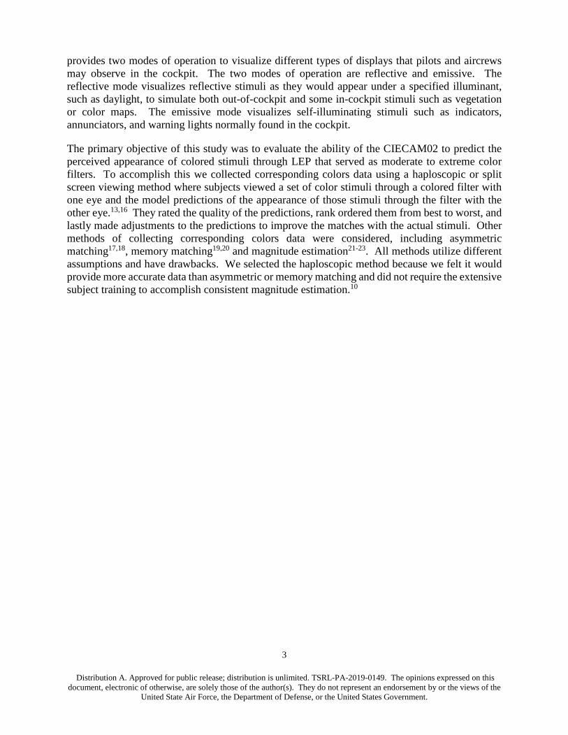
2.2 Filters The colored filters for the visual evaluations consisted of four Commercial-off-the-Shelf (COTS) LEP devices in spectacle format. We selected the filters in order to push the limits of the CIECAM02 predictions for both luminance and chromaticity. These LEP blocked different regions of the visible spectrum and reduced the overall luminance by approximately 50%. Specifically, one blocked long wavelengths (648 ± 11 nm) and was a red blocker (RBlkr), one blocked medium wavelengths (527 ± 15 nm) and was a green blocker (GBlkr). The other two LEP were blue blockers with one that blocked all wavelengths < ~ 530 nm except for a narrow band centered around 427 ± 13 nm (BBlkr1) and the other blocked all wavelengths <544 nm (BBlkr2). We used a 40% transmission neutral density filter, with a photopic luminous transmission (PLT) slightly lower than the lowest PLT of the LEP (range 47% - 56%) as a conservative control. In Figure 1, the transmission spectra of ND40% and the LEP are plotted together with the emission spectra of the red, green and blue channels of the color monitor (top panel) and with the normalized sensitivity spectra of the long (L), middle (M) and short (S) wavelength sensitive-cone photoreceptors (bottom panel). The purpose of the two graphs is to illustrate interaction between the transmission spectra of the LEP and the RGB channels of the monitor and the cone sensitivities. For example, in the top panel one can see that BBlkr2 blocks the output of the B monitor channel. At the same time, we see that it will deprive the S-cones of input (bottom panel) regardless of whether or not short-wavelength light is available. In contrast, BBlkr1 blocks less middle wavelengths and also transmits some light at short wavelengths centered on 430 nm.
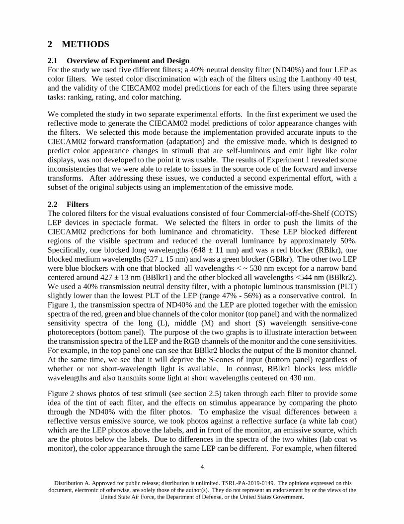
Figure 2 shows photos of test stimuli (see section 2.5) taken through each filter to provide some idea of the tint of each filter, and the effects on stimulus appearance by comparing the photo through the ND40% with the filter photos. To emphasize the visual differences between a reflective versus emissive source, we took photos against a reflective surface (a white lab coat) which are the LEP photos above the labels, and in front of the monitor, an emissive source, which are the photos below the labels. Due to differences in the spectra of the two whites (lab coat vs monitor), the color appearance through the same LEP can be different. For example, when filtered
5
Distribution A. Approved for public release; distribution is unlimited. TSRL-PA-2019-0149. The opinions expressed on this document, electronic of otherwise, are solely those of the author(s). They do not represent an endorsement by or the views of the
United State Air Force, the Department of Defense, or the United States Government.
through the green blocker (GBlkr), the white reflective lab coat appears orange while the white of the emissive monitor appears purple/magenta. These photographs emphasize why it is important to model the color appearance of reflective and emissive sources differently in CIECAM02.
Figure 1. Transmission spectra of COTS filters plotted against output of the R, G, and B monitor channels (top panel) and relative sensitivity of the L-, M-, and S-cones (bottom
panel)
6
Distribution A. Approved for public release; distribution is unlimited. TSRL-PA-2019-0149. The opinions expressed on this document, electronic of otherwise, are solely those of the author(s). They do not represent an endorsement by or the views of the
United State Air Force, the Department of Defense, or the United States Government.
Figure 2. ND40% and COTS filters (reflective lab coat above labels and emissive monitor below labels)
2.3 Lanthony 40 Hue Test The Lanthony 40 Hue test is an arrangement test where subjects arrange ten color caps in each of four rows in an orderly progression. We had subjects sort caps in each row separately under a daylight illuminator (Richmond Products model 1339R) while viewing them binocularly through each LEP and the ND40%. On the first test day of Experiment 1 we had all subjects complete the test with the ND40%. On each of the four subsequent test days we had them take the test again with the colored LEP that had been assigned for that day. The Score Index (SI) was computed from the cap orders using standard methods in an excel spreadsheet. The SI is based on the number and size of cap transposition errors with lower scores indicating better performance on the test. SI scores less than ten are considered to be in the normal range with higher scores indicating some level of color vision defect.

7
Distribution A. Approved for public release; distribution is unlimited. TSRL-PA-2019-0149. The opinions expressed on this document, electronic of otherwise, are solely those of the author(s). They do not represent an endorsement by or the views of the
United State Air Force, the Department of Defense, or the United States Government.
Figure 3. Lanthony 40 Hue Test
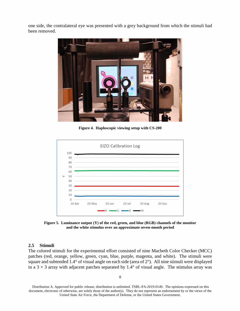
2.4 Display Parameters In both experiments, subjects performed each of the model validity tasks in a successive-haploscopic display scenario. The haploscopic method assumes adaptation takes place independently in both eyes, which dominates for sensory processes.24 To achieve this, we divided the display vertically with a black foam barrier and had subjects view each side of the display through viewing tubes with attached eyecups to provide the haploscopic view. We used a chin and head rest to stabilize eye alignment with the filter and the viewing tubes. Figure 4 shows the setup with the eye-cups, tubes, and dividing septum.
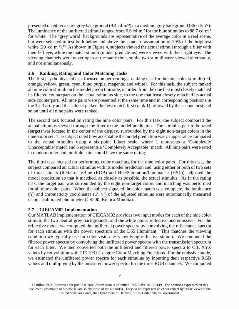
The display we used for stimulus presentation was an EIZO ColorEdge CG318, 4K LED monitor. We selected it because of stated manufacturer specifications of overall color additivity, spatial homogeneity, and stability over time. It also allowed us to display the Adobe RGB space, which has a larger color gamut and can display more colors than sRGB space. These properties were verified by taking spectral measurements (Y, u’, v’) across the entire viewing field of the monitor with a high resolution LumiCam 1300 Imaging Photometer/Colorimeter (Instrument Systems) and by generating color mixtures of red, green and blue to determine if the sum provided the same output as the white setting. We then cross-calibrated all measurements with the CS-200, which we later used to measure subject color matches. Figure 5 illustrates the stability of the display over the time-course of the experiments.
On the left side of the display screen, we presented the actual stimuli which were viewed with the left eye looking through a filter (ND or LEP). On the right side of the screen we displayed the CIECAM02 prediction of stimuli appearance through the filter (see Section 2.7 for details of stimuli design). Subjects viewed only one side at a time, and used a mouse to freely switch between views (eyes), to perform stimulus adjustments, and to make decisions. While viewing
8
Distribution A. Approved for public release; distribution is unlimited. TSRL-PA-2019-0149. The opinions expressed on this document, electronic of otherwise, are solely those of the author(s). They do not represent an endorsement by or the views of the
United State Air Force, the Department of Defense, or the United States Government.
one side, the contralateral eye was presented with a grey background from which the stimuli had been removed.
Figure 4. Haploscopic viewing setup with CS-200
Figure 5. Luminance output (Y) of the red, green, and blue (RGB) channels of the monitor and the white stimulus over an approximate seven-month period
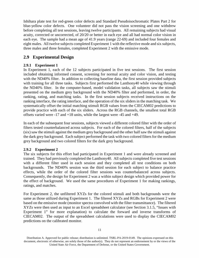
2.5 Stimuli The colored stimuli for the experimental effort consisted of nine Macbeth Color Checker (MCC) patches (red, orange, yellow, green, cyan, blue, purple, magenta, and white). The stimuli were square and subtended 1.4° of visual angle on each side (area of 2°). All nine stimuli were displayed in a 3 × 3 array with adjacent patches separated by 1.4° of visual angle. The stimulus array was
9
Distribution A. Approved for public release; distribution is unlimited. TSRL-PA-2019-0149. The opinions expressed on this document, electronic of otherwise, are solely those of the author(s). They do not represent an endorsement by or the views of the
United State Air Force, the Department of Defense, or the United States Government.
presented on either a dark grey background (9.4 cd·m-²) or a medium grey background (36 cd·m-²). The luminance of the unfiltered stimuli ranged from 6.6 cd·m-² for the blue stimulus to 88.7 cd·m-² for white. The ‘grey world’ backgrounds are representative of the average color in a real scene, but were selected to test both below and above the standard assumption of 20% of the brightest white (20 cd·m-²).10 As shown in Figure 4, subjects viewed the actual stimuli through a filter with their left eye, while the match stimuli (model predictions) were viewed with their right eye. The viewing channels were never open at the same time, so the two stimuli were viewed alternately, and not simultaneously.
2.6 Ranking, Rating and Color Matching Tasks The first psychophysical task focused on performing a ranking task for the nine color stimuli (red, orange, yellow, green, cyan, blue, purple, magenta, and white). For this task, the subject ranked all nine color stimuli on the model prediction side, in order, from the one that most closely matched its filtered counterpart on the actual stimulus side, to the one that least closely matched its actual side counterpart. All nine pairs were presented at the same time and in corresponding positions in the 3 x 3 array and the subject picked the best match first (rank 1) followed by the second best and so on until all nine pairs were ranked.
The second task focused on rating the nine color pairs. For this task, the subject compared the actual stimulus viewed through the filter to the model prediction. The stimulus pair to be rated (target) was located in the center of the display, surrounded by the eight non-target colors in the nine-color set. The subject rated how acceptable the model prediction was in appearance compared to the actual stimulus using a six-point Likert scale, where 1 represents a ‘Completely Unacceptable’ match and 6 represents a ‘Completely Acceptable’ match. All nine pairs were rated in random order and multiple pairs could have the same rating.
The third task focused on performing color matching for the nine color pairs. For this task, the subject compared an actual stimulus with its model prediction and, using either or both of two sets of three sliders (Red/Green/Blue (RGB) and Hue/Saturation/Luminance (HSL)), adjusted the model prediction so that it matched, as closely as possible, the actual stimulus. As in the rating task, the target pair was surrounded by the eight non-target colors and matching was performed for all nine color pairs. When the subject signaled the color match was complete, the luminance (Y) and chromaticity coordinates (u’, v’) of the adjusted stimulus were automatically measured using a calibrated photometer (CS200, Konica Minolta).
2.7 CIECAM02 Implementation Our MATLAB implementation of CIECAM02 provides two input modes for each of the nine color stimuli, the two neutral grey backgrounds, and the white point: reflective and emissive. For the reflective mode, we computed the unfiltered power spectra by convolving the reflectance spectra for each stimulus with the power spectrum of the D65 illuminant. This matches the viewing condition we typically use for color vision tests involving reflective stimuli. We computed the filtered power spectra by convolving the unfiltered power spectra with the transmission spectrum for each filter. We then converted both the unfiltered and filtered power spectra to CIE XYZ values by convolution with CIE 1931 2-degree Color Matching Functions. For the emissive mode, we estimated the unfiltered power spectra for each stimulus by inputting their respective RGB values and multiplying by the measured power spectra for the three RGB channels. We computed
10
Distribution A. Approved for public release; distribution is unlimited. TSRL-PA-2019-0149. The opinions expressed on this document, electronic of otherwise, are solely those of the author(s). They do not represent an endorsement by or the views of the
United State Air Force, the Department of Defense, or the United States Government.
the filtered power spectra and then converted it, and the unfiltered power spectra to XYZ values using the procedure described for the reflective mode.
We displayed the unfiltered stimuli on the left side of the monitor simply by transforming the XYZ values to Adobe RGB values using image-processing functions. To display the adapted (model predictions) stimuli we used the forward and inverse CIECAM02 modules for both modes. The forward module converts the filtered stimuli from XYZ values to perceptual correlates such as lightness (J), chroma (C), and hue angle (h), that take chromatic adaption into account, while the inverse transform module converts the model factors back to adapted XYZ values, which are then converted to Adobe RGB values that control the presentation of the stimuli on to the calibrated display. In all cases, we verified measurements of monitor luminance and chromaticity values against calculations.
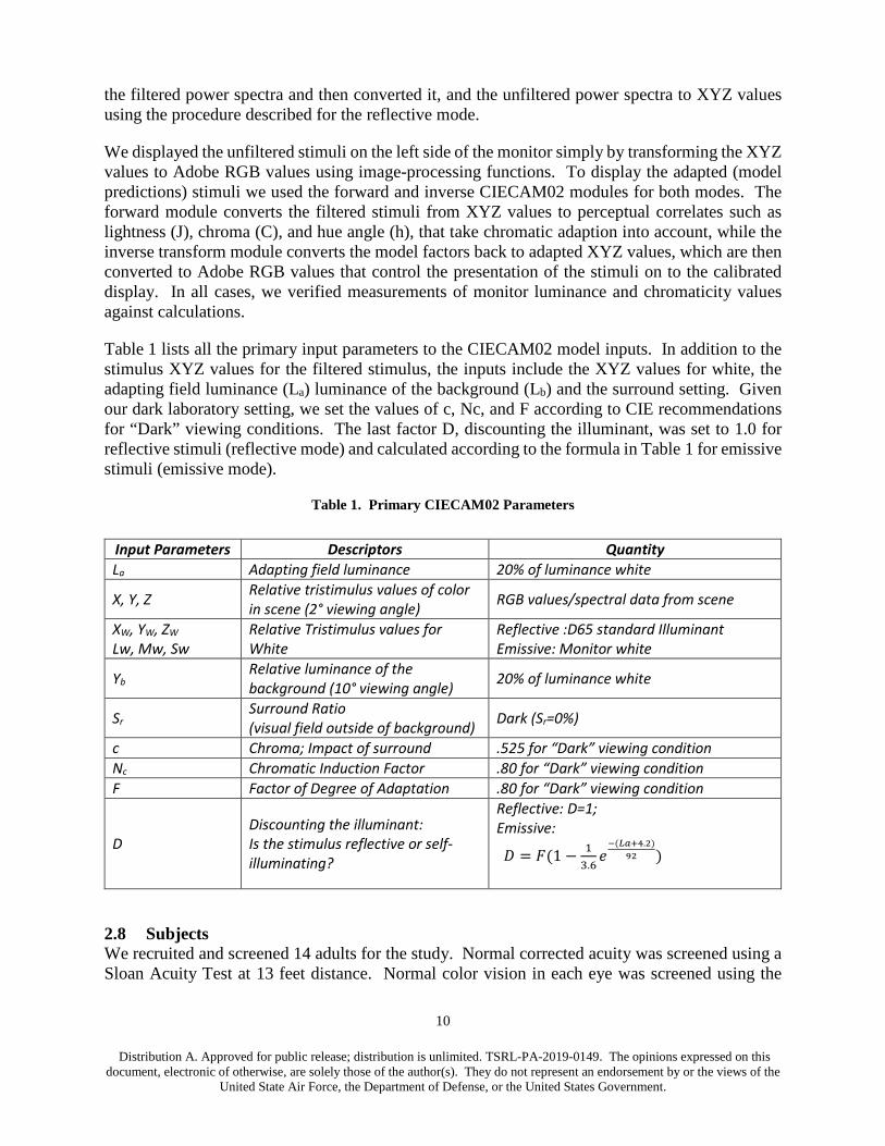
Table 1 lists all the primary input parameters to the CIECAM02 model inputs. In addition to the stimulus XYZ values for the filtered stimulus, the inputs include the XYZ values for white, the adapting field luminance (La) luminance of the background (Lb) and the surround setting. Given our dark laboratory setting, we set the values of c, Nc, and F according to CIE recommendations for “Dark” viewing conditions. The last factor D, discounting the illuminant, was set to 1.0 for reflective stimuli (reflective mode) and calculated according to the formula in Table 1 for emissive stimuli (emissive mode).
Table 1. Primary CIECAM02 Parameters
Input Parameters Descriptors Quantity La Adapting field luminance 20% of luminance white
X, Y, Z Relative tristimulus values of color in scene (2° viewing angle) RGB values/spectral data from scene
XW, YW, ZW
Lw, Mw, Sw Relative Tristimulus values for White
Reflective :D65 standard Illuminant Emissive: Monitor white
Yb Relative luminance of the background (10° viewing angle) 20% of luminance white
Sr Surround Ratio (visual field outside of background) Dark (Sr=0%)
c Chroma; Impact of surround .525 for “Dark” viewing condition Nc Chromatic Induction Factor .80 for “Dark” viewing condition F Factor of Degree of Adaptation .80 for “Dark” viewing condition
D Discounting the illuminant: Is the stimulus reflective or self-illuminating?
Reflective: D=1; Emissive:
𝐷𝐷 = 𝐹𝐹(1 − 13.6𝑒𝑒−(𝐿𝐿𝐿𝐿+4.2)
92 )
2.8 Subjects We recruited and screened 14 adults for the study. Normal corrected acuity was screened using a Sloan Acuity Test at 13 feet distance. Normal color vision in each eye was screened using the
11
Distribution A. Approved for public release; distribution is unlimited. TSRL-PA-2019-0149. The opinions expressed on this document, electronic of otherwise, are solely those of the author(s). They do not represent an endorsement by or the views of the
United State Air Force, the Department of Defense, or the United States Government.
Ishihara plate test for red-green color defects and Standard Pseudoisochromatic Plates Part 2 for blue-yellow color defects. One volunteer did not pass the vision screening and one withdrew before completing all test sessions, leaving twelve participants. All remaining subjects had visual acuity, corrected or uncorrected, of 20/20 or better in each eye and all had normal color vision in each eye. The sample had a mean age of 41.9 years (range 22-69) and included four females and eight males. All twelve subjects completed Experiment 1 with the reflective mode and six subjects, three males and three females, completed Experiment 2 with the emissive mode.
2.9 Experimental Design
2.9.1 Experiment 1 In Experiment 1, each of the 12 subjects participated in five test sessions. The first session included obtaining informed consent, screening for normal acuity and color vision, and testing with the ND40% filter. In addition to collecting baseline data, the first session provided subjects with training for all three tasks. Subjects first performed the Lanthony40 while viewing through the ND40% filter. In the computer-based, model validation tasks, all subjects saw the stimuli presented on the medium grey background with the ND40% filter and performed, in order, the ranking, rating, and matching tasks. In the first session subjects received instructions on the ranking interface, the rating interface, and the operation of the six sliders in the matching task. We systematically offset the initial matching stimuli RGB values from the CIECAM02 predictions to provide practice with each of the six sliders. Across the RGB channels, the smallest total RGB offsets varied were -17 and +18 units, while the largest were -45 and +49.
In each of the subsequent four sessions, subjects viewed a different colored filter with the order of filters tested counterbalanced across subjects. For each of the colored filters, half of the subjects (six) saw the stimuli against the medium grey background and the other half saw the stimuli against the dark grey background. Each subject performed the task with two colored filters for the medium grey background and two colored filters for the dark grey background.
2.9.2 Experiment 2 The six subjects for this effort had participated in Experiment 1 and were already screened and trained. They had previously completed the Lanthony40. All subjects completed five test sessions with a different filter used in each session and they completed all test conditions on both backgrounds. The ND40% session was the third session for each subject to balance practice effects, while the order of the colored filter sessions was counterbalanced across subjects. Consequently, the design for Experiment 2 was a within subject design which provided power for the effect of background. We used the same procedures of Experiment 1 for making rankings, ratings, and matches.
For Experiment 2, the unfiltered XYZs for the colored stimuli and both backgrounds were the same as those utilized during Experiment 1. The filtered XYZs and RGBs for Experiment 2 were based on the emissive mode (monitor spectra convolved with the filter transmittance). The filtered XYZs were then used as input to an Excel spreadsheet calculator (see Section 3.1.5, “Issues with Experiment 1” for more explanation) to calculate the forward and inverse transforms of CIECAM02. The output of the spreadsheet calculations were used to display the CIECAM02 predictions on the calibrated monitor.
12
Distribution A. Approved for public release; distribution is unlimited. TSRL-PA-2019-0149. The opinions expressed on this document, electronic of otherwise, are solely those of the author(s). They do not represent an endorsement by or the views of the
United State Air Force, the Department of Defense, or the United States Government.
3 Results
3.1 Experiment 1
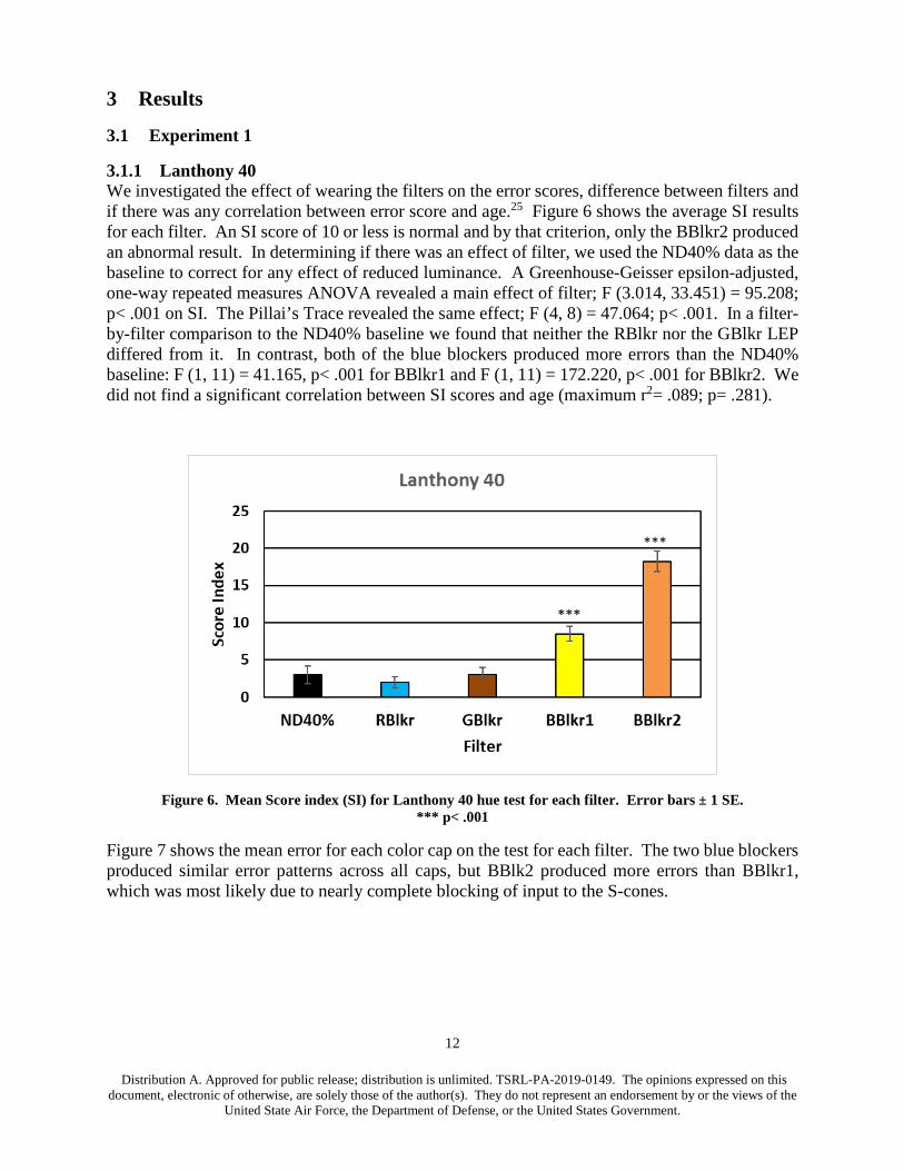
3.1.1 Lanthony 40 We investigated the effect of wearing the filters on the error scores, difference between filters and if there was any correlation between error score and age.25 Figure 6 shows the average SI results for each filter. An SI score of 10 or less is normal and by that criterion, only the BBlkr2 produced an abnormal result. In determining if there was an effect of filter, we used the ND40% data as the baseline to correct for any effect of reduced luminance. A Greenhouse-Geisser epsilon-adjusted, one-way repeated measures ANOVA revealed a main effect of filter; F (3.014, 33.451) = 95.208; p< .001 on SI. The Pillai’s Trace revealed the same effect; F (4, 8) = 47.064; p< .001. In a filter-by-filter comparison to the ND40% baseline we found that neither the RBlkr nor the GBlkr LEP differed from it. In contrast, both of the blue blockers produced more errors than the ND40% baseline: F (1, 11) = 41.165, p< .001 for BBlkr1 and F (1, 11) = 172.220, p< .001 for BBlkr2. We did not find a significant correlation between SI scores and age (maximum r2= .089; p= .281).
Figure 6. Mean Score index (SI) for Lanthony 40 hue test for each filter. Error bars ± 1 SE. *** p< .001
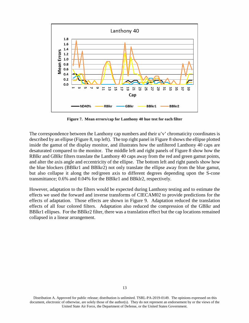
Figure 7 shows the mean error for each color cap on the test for each filter. The two blue blockers produced similar error patterns across all caps, but BBlk2 produced more errors than BBlkr1, which was most likely due to nearly complete blocking of input to the S-cones.
13
Distribution A. Approved for public release; distribution is unlimited. TSRL-PA-2019-0149. The opinions expressed on this document, electronic of otherwise, are solely those of the author(s). They do not represent an endorsement by or the views of the
United State Air Force, the Department of Defense, or the United States Government.
Figure 7. Mean errors/cap for Lanthony 40 hue test for each filter
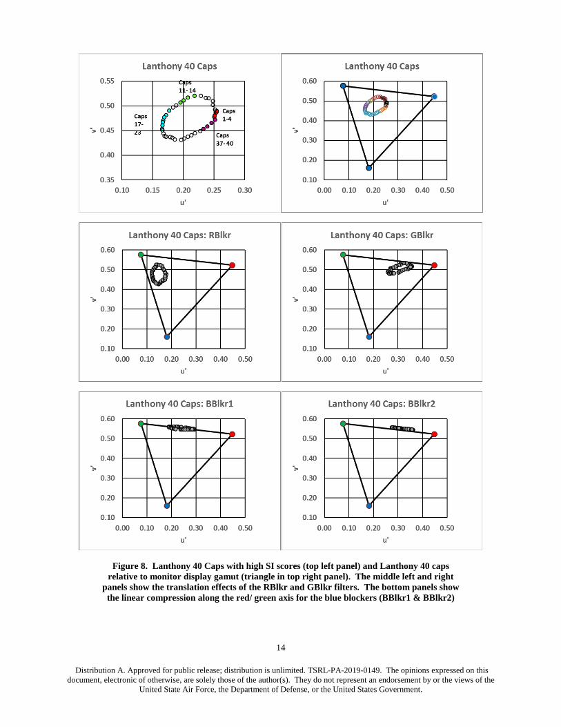
The correspondence between the Lanthony cap numbers and their u’v’ chromaticity coordinates is described by an ellipse (Figure 8, top left). The top right panel in Figure 8 shows the ellipse plotted inside the gamut of the display monitor, and illustrates how the unfiltered Lanthony 40 caps are desaturated compared to the monitor. The middle left and right panels of Figure 8 show how the RBlkr and GBlkr filters translate the Lanthony 40 caps away from the red and green gamut points, and alter the axis angle and eccentricity of the ellipse. The bottom left and right panels show how the blue blockers (BBlkr1 and BBlkr2) not only translate the ellipse away from the blue gamut, but also collapse it along the red/green axis to different degrees depending upon the S-cone transmittance; 0.6% and 0.04% for the BBlkr1 and BBklr2, respectively.
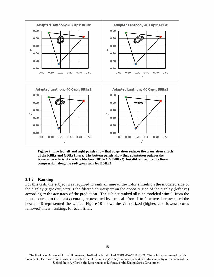
However, adaptation to the filters would be expected during Lanthony testing and to estimate the effects we used the forward and inverse transforms of CIECAM02 to provide predictions for the effects of adaptation. Those effects are shown in Figure 9. Adaptation reduced the translation effects of all four colored filters. Adaptation also reduced the compression of the GBlkr and BBlkr1 ellipses. For the BBlkr2 filter, there was a translation effect but the cap locations remained collapsed in a linear arrangement.
14
Distribution A. Approved for public release; distribution is unlimited. TSRL-PA-2019-0149. The opinions expressed on this document, electronic of otherwise, are solely those of the author(s). They do not represent an endorsement by or the views of the
United State Air Force, the Department of Defense, or the United States Government.
Figure 8. Lanthony 40 Caps with high SI scores (top left panel) and Lanthony 40 caps relative to monitor display gamut (triangle in top right panel). The middle left and right
panels show the translation effects of the RBlkr and GBlkr filters. The bottom panels show the linear compression along the red/ green axis for the blue blockers (BBlkr1 & BBlkr2)
15
Distribution A. Approved for public release; distribution is unlimited. TSRL-PA-2019-0149. The opinions expressed on this document, electronic of otherwise, are solely those of the author(s). They do not represent an endorsement by or the views of the
United State Air Force, the Department of Defense, or the United States Government.
Figure 9. The top left and right panels show that adaptation reduces the translation effects of the RBlkr and GBlkr filters. The bottom panels show that adaptation reduces the translation effects of the blue blockers (BBlkr1 & BBlkr2), but did not reduce the linear compression along the red/ green axis for BBlkr2
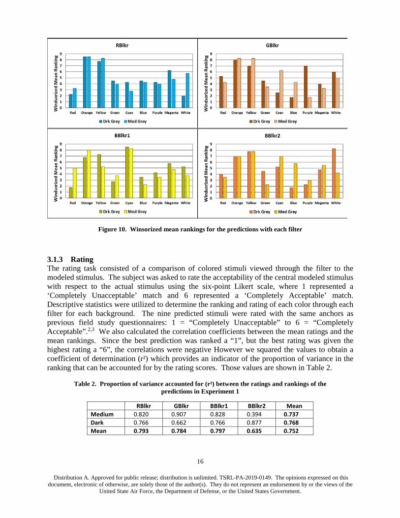
3.1.2 Ranking For this task, the subject was required to rank all nine of the color stimuli on the modeled side of the display (right eye) versus the filtered counterpart on the opposite side of the display (left eye) according to the accuracy of the prediction. The subject ranked all nine modeled stimuli from the most accurate to the least accurate, represented by the scale from 1 to 9, where 1 represented the best and 9 represented the worst. Figure 10 shows the Winsorized (highest and lowest scores removed) mean rankings for each filter.
16
Distribution A. Approved for public release; distribution is unlimited. TSRL-PA-2019-0149. The opinions expressed on this document, electronic of otherwise, are solely those of the author(s). They do not represent an endorsement by or the views of the
United State Air Force, the Department of Defense, or the United States Government.
Figure 10. Winsorized mean rankings for the predictions with each filter
3.1.3 Rating The rating task consisted of a comparison of colored stimuli viewed through the filter to the modeled stimulus. The subject was asked to rate the acceptability of the central modeled stimulus with respect to the actual stimulus using the six-point Likert scale, where 1 represented a ‘Completely Unacceptable’ match and 6 represented a ‘Completely Acceptable’ match. Descriptive statistics were utilized to determine the ranking and rating of each color through each filter for each background. The nine predicted stimuli were rated with the same anchors as previous field study questionnaires: 1 = “Completely Unacceptable” to 6 = “Completely Acceptable”.2,3 We also calculated the correlation coefficients between the mean ratings and the mean rankings. Since the best prediction was ranked a “1”, but the best rating was given the highest rating a “6”, the correlations were negative However we squared the values to obtain a coefficient of determination (r²) which provides an indicator of the proportion of variance in the ranking that can be accounted for by the rating scores. Those values are shown in Table 2.
Table 2. Proportion of variance accounted for (r²) between the ratings and rankings of the predictions in Experiment 1
RBlkr GBlkr BBlkr1 BBlkr2 Mean Medium 0.820 0.907 0.828 0.394 0.737 Dark 0.766 0.662 0.766 0.877 0.768 Mean 0.793 0.784 0.797 0.635 0.752
17
Distribution A. Approved for public release; distribution is unlimited. TSRL-PA-2019-0149. The opinions expressed on this document, electronic of otherwise, are solely those of the author(s). They do not represent an endorsement by or the views of the
United State Air Force, the Department of Defense, or the United States Government.
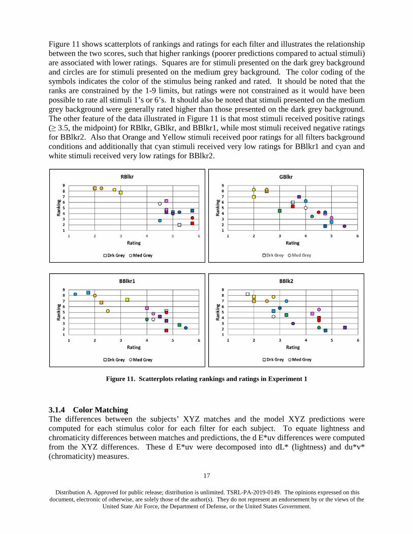
Figure 11 shows scatterplots of rankings and ratings for each filter and illustrates the relationship between the two scores, such that higher rankings (poorer predictions compared to actual stimuli) are associated with lower ratings. Squares are for stimuli presented on the dark grey background and circles are for stimuli presented on the medium grey background. The color coding of the symbols indicates the color of the stimulus being ranked and rated. It should be noted that the ranks are constrained by the 1-9 limits, but ratings were not constrained as it would have been possible to rate all stimuli 1’s or 6’s. It should also be noted that stimuli presented on the medium grey background were generally rated higher than those presented on the dark grey background. The other feature of the data illustrated in Figure 11 is that most stimuli received positive ratings (≥ 3.5, the midpoint) for RBlkr, GBlkr, and BBlkr1, while most stimuli received negative ratings for BBlkr2. Also that Orange and Yellow stimuli received poor ratings for all filters background conditions and additionally that cyan stimuli received very low ratings for BBlkr1 and cyan and white stimuli received very low ratings for BBlkr2.
Figure 11. Scatterplots relating rankings and ratings in Experiment 1
3.1.4 Color Matching The differences between the subjects’ XYZ matches and the model XYZ predictions were computed for each stimulus color for each filter for each subject. To equate lightness and chromaticity differences between matches and predictions, the d E*uv differences were computed from the XYZ differences. These d E*uv were decomposed into dL* (lightness) and du*v* (chromaticity) measures.
18
Distribution A. Approved for public release; distribution is unlimited. TSRL-PA-2019-0149. The opinions expressed on this document, electronic of otherwise, are solely those of the author(s). They do not represent an endorsement by or the views of the
United State Air Force, the Department of Defense, or the United States Government.
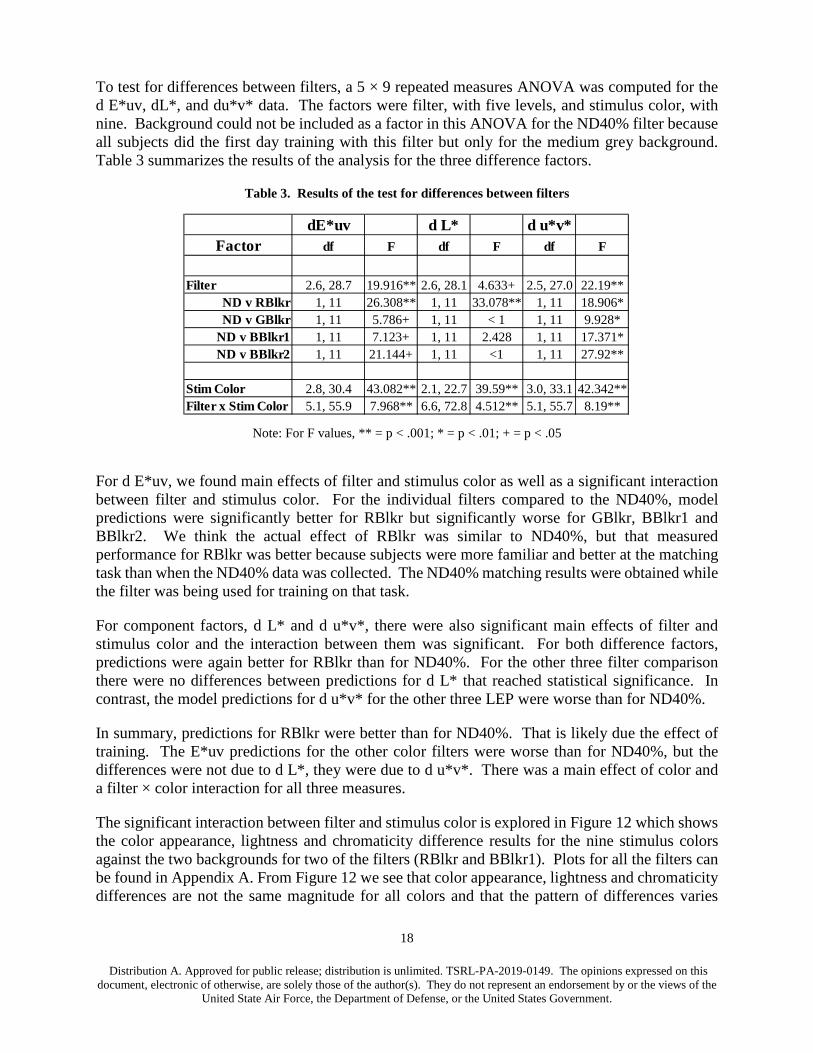
To test for differences between filters, a 5 × 9 repeated measures ANOVA was computed for the d E*uv, dL*, and du*v* data. The factors were filter, with five levels, and stimulus color, with nine. Background could not be included as a factor in this ANOVA for the ND40% filter because all subjects did the first day training with this filter but only for the medium grey background. Table 3 summarizes the results of the analysis for the three difference factors.
Table 3. Results of the test for differences between filters
Note: For F values, ** = p < .001; * = p < .01; + = p < .05
For d E*uv, we found main effects of filter and stimulus color as well as a significant interaction between filter and stimulus color. For the individual filters compared to the ND40%, model predictions were significantly better for RBlkr but significantly worse for GBlkr, BBlkr1 and BBlkr2. We think the actual effect of RBlkr was similar to ND40%, but that measured performance for RBlkr was better because subjects were more familiar and better at the matching task than when the ND40% data was collected. The ND40% matching results were obtained while the filter was being used for training on that task.
For component factors, d L* and d u*v*, there were also significant main effects of filter and stimulus color and the interaction between them was significant. For both difference factors, predictions were again better for RBlkr than for ND40%. For the other three filter comparison there were no differences between predictions for d L* that reached statistical significance. In contrast, the model predictions for d u*v* for the other three LEP were worse than for ND40%.
In summary, predictions for RBlkr were better than for ND40%. That is likely due the effect of training. The E*uv predictions for the other color filters were worse than for ND40%, but the differences were not due to d L*, they were due to d u*v*. There was a main effect of color and a filter × color interaction for all three measures.
The significant interaction between filter and stimulus color is explored in Figure 12 which shows the color appearance, lightness and chromaticity difference results for the nine stimulus colors against the two backgrounds for two of the filters (RBlkr and BBlkr1). Plots for all the filters can be found in Appendix A. From Figure 12 we see that color appearance, lightness and chromaticity differences are not the same magnitude for all colors and that the pattern of differences varies
dE*uv d L* d u*v*Factor df F df F df F
Filter 2.6, 28.7 19.916** 2.6, 28.1 4.633+ 2.5, 27.0 22.19**ND v RBlkr 1, 11 26.308** 1, 11 33.078** 1, 11 18.906*ND v GBlkr 1, 11 5.786+ 1, 11 < 1 1, 11 9.928*
ND v BBlkr1 1, 11 7.123+ 1, 11 2.428 1, 11 17.371*ND v BBlkr2 1, 11 21.144+ 1, 11 <1 1, 11 27.92**
Stim Color 2.8, 30.4 43.082** 2.1, 22.7 39.59** 3.0, 33.1 42.342**Filter x Stim Color 5.1, 55.9 7.968** 6.6, 72.8 4.512** 5.1, 55.7 8.19**
19
Distribution A. Approved for public release; distribution is unlimited. TSRL-PA-2019-0149. The opinions expressed on this document, electronic of otherwise, are solely those of the author(s). They do not represent an endorsement by or the views of the
United State Air Force, the Department of Defense, or the United States Government.
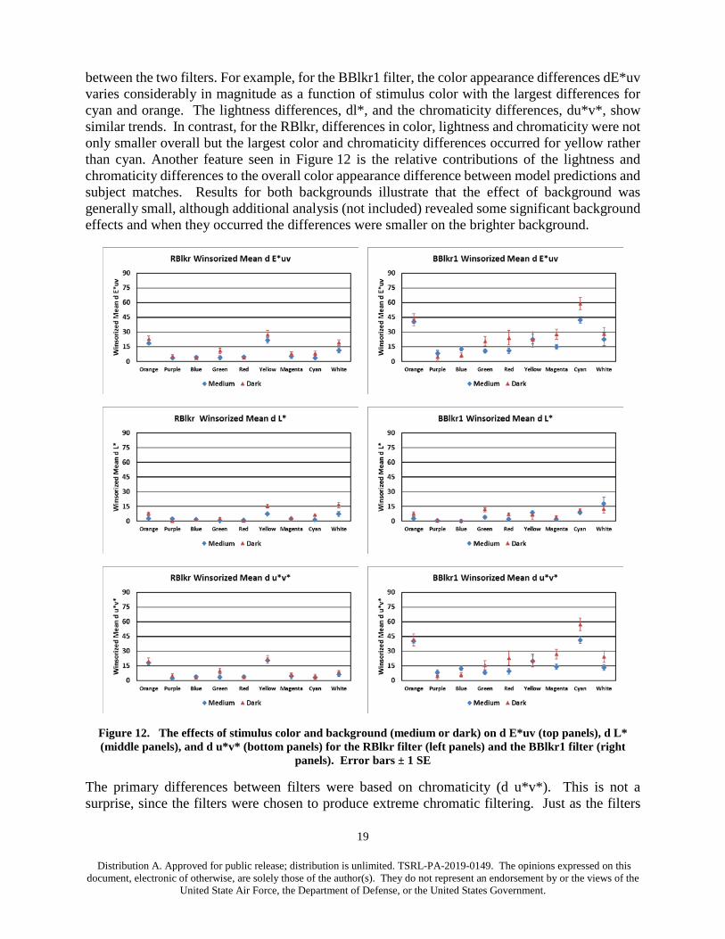
between the two filters. For example, for the BBlkr1 filter, the color appearance differences dE*uv varies considerably in magnitude as a function of stimulus color with the largest differences for cyan and orange. The lightness differences, dl*, and the chromaticity differences, du*v*, show similar trends. In contrast, for the RBlkr, differences in color, lightness and chromaticity were not only smaller overall but the largest color and chromaticity differences occurred for yellow rather than cyan. Another feature seen in Figure 12 is the relative contributions of the lightness and chromaticity differences to the overall color appearance difference between model predictions and subject matches. Results for both backgrounds illustrate that the effect of background was generally small, although additional analysis (not included) revealed some significant background effects and when they occurred the differences were smaller on the brighter background.
Figure 12. The effects of stimulus color and background (medium or dark) on d E*uv (top panels), d L* (middle panels), and d u*v* (bottom panels) for the RBlkr filter (left panels) and the BBlkr1 filter (right
panels). Error bars ± 1 SE
The primary differences between filters were based on chromaticity (d u*v*). This is not a surprise, since the filters were chosen to produce extreme chromatic filtering. Just as the filters
20
Distribution A. Approved for public release; distribution is unlimited. TSRL-PA-2019-0149. The opinions expressed on this document, electronic of otherwise, are solely those of the author(s). They do not represent an endorsement by or the views of the
United State Air Force, the Department of Defense, or the United States Government.
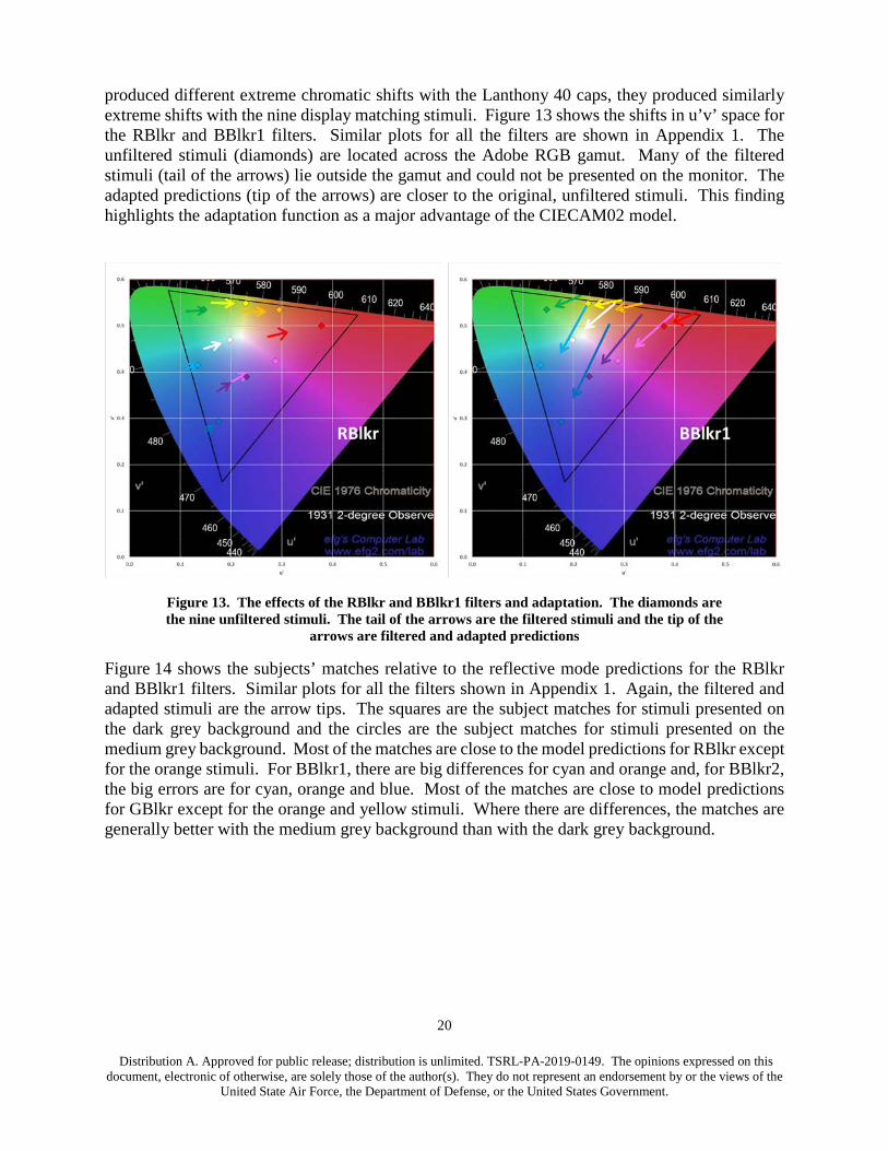
produced different extreme chromatic shifts with the Lanthony 40 caps, they produced similarly extreme shifts with the nine display matching stimuli. Figure 13 shows the shifts in u’v’ space for the RBlkr and BBlkr1 filters. Similar plots for all the filters are shown in Appendix 1. The unfiltered stimuli (diamonds) are located across the Adobe RGB gamut. Many of the filtered stimuli (tail of the arrows) lie outside the gamut and could not be presented on the monitor. The adapted predictions (tip of the arrows) are closer to the original, unfiltered stimuli. This finding highlights the adaptation function as a major advantage of the CIECAM02 model.
Figure 13. The effects of the RBlkr and BBlkr1 filters and adaptation. The diamonds are the nine unfiltered stimuli. The tail of the arrows are the filtered stimuli and the tip of the
arrows are filtered and adapted predictions
Figure 14 shows the subjects’ matches relative to the reflective mode predictions for the RBlkr and BBlkr1 filters. Similar plots for all the filters shown in Appendix 1. Again, the filtered and adapted stimuli are the arrow tips. The squares are the subject matches for stimuli presented on the dark grey background and the circles are the subject matches for stimuli presented on the medium grey background. Most of the matches are close to the model predictions for RBlkr except for the orange stimuli. For BBlkr1, there are big differences for cyan and orange and, for BBlkr2, the big errors are for cyan, orange and blue. Most of the matches are close to model predictions for GBlkr except for the orange and yellow stimuli. Where there are differences, the matches are generally better with the medium grey background than with the dark grey background.

21
Distribution A. Approved for public release; distribution is unlimited. TSRL-PA-2019-0149. The opinions expressed on this document, electronic of otherwise, are solely those of the author(s). They do not represent an endorsement by or the views of the
United State Air Force, the Department of Defense, or the United States Government.
Figure 14. Subject matches relative to filtered and adapted predictions (arrow tips) for RBlkr and BBlkr1 filters. Squares are matches with the dark grey background and circles
are matches with the medium grey background
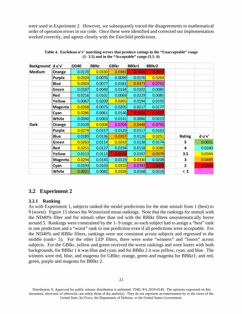
To link the Rating and Matching data, Ratings were regressed against Winsorized luminance matching errors (delta Y) and Winsorized matching chromaticity errors (Euclidean u’v’). Ratings were better predicted by the chromaticity errors (r²= 0.491) than by luminance errors (r²= 0.131). The rating scale was anchored with 6 = “Completely Acceptable” and 1 = “Completely Unacceptable”. The regression equation (Rating= -47.856* Euclidean u’v’ + 5.148) was used to estimate the Euclidean u’v’ error that would produce ratings of 5, 4, 3.5 (the Acceptable / Unacceptable boundary), 3 and 2. u’v’ provided a better fit than u*v*. Table 4Table 2 shows the error estimates for each stimulus color on each background with each filter. All the stimuli were in the “Acceptable” range for ND40% and RBlkr. For GBlkr, BBlkr1, and BBlkr2, there were four, five, and six stimuli in the “Unacceptable” range, respectively.
3.1.5 Issues with Experiment 1 Reviewing Experiment 1 results indicated that there were large differences between the subject matches and the filtered and adapted predictions. Subsequent tests of the software implantation revealed several errors in the code calculating the filtered, unadapted stimuli. These errors were corrected and incorporated into the code for the emissive mode we used for Experiment 2. To test the debugged emissive mode implementation, we investigated whether it provided better fits than the reflective mode for the stimuli presented on the calibrated monitor. We found that relative to the Experiment 1 subject matches, emissive mode predictions were usually worse than the reflective mode predictions, suggesting there may still be problems in the forward and inverse adaptation functions To test the accuracy of the forward and inverse transform implementation we compared emissive mode predictions of Experiment 1 data to those we computed using a publicly available Excel spreadsheet prepared by Mark Fairchild to generate CIECAM02 predictions for given emissive stimulus sample inputs.26 We spent a considerable amount of effort trying to debug our implementation, but found the Fairchild predictions to be significantly more accurate than our emissive mode predictions. In the interests of time, the Excel-based calculations
22
Distribution A. Approved for public release; distribution is unlimited. TSRL-PA-2019-0149. The opinions expressed on this document, electronic of otherwise, are solely those of the author(s). They do not represent an endorsement by or the views of the
United State Air Force, the Department of Defense, or the United States Government.
were used in Experiment 2. However, we subsequently traced the disagreements to mathematical order of operation errors in our code. Once these were identified and corrected our implementation worked correctly, and agrees closely with the Fairchild predictions.
Table 4. Euclidean u’v’ matching errors that produce ratings in the “Unacceptable” range
(1- 3.5) and in the “Acceptable” range (3.5- 6)
3.2 Experiment 2
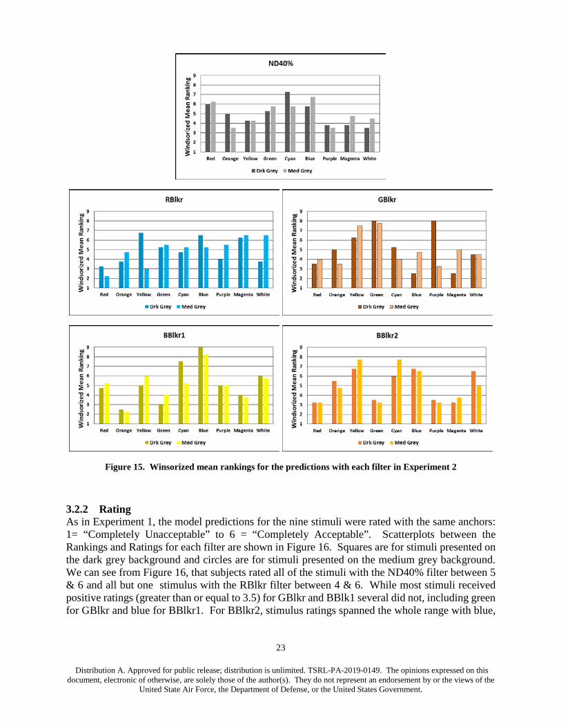
3.2.1 Ranking As with Experiment 1, subjects ranked the model predictions for the nine stimuli from 1 (best) to 9 (worst). Figure 15 shows the Winsorized mean rankings. Note that the rankings for stimuli with the ND40% filter and for stimuli other than red with the RBlkr filters unsystematically hover around 5. Rankings were constrained by the 1- 9 range, so each subject had to assign a “best” rank to one prediction and a “worst” rank to one prediction even if all predictions were acceptable. For the ND40% and RBlkr filters, rankings were not consistent across subjects and regressed to the middle (rank= 5). For the other LEP filters, there were some “winners” and “losers” across subjects. For the GBlkr, yellow and green received the worst rankings and were losers with both backgrounds, for BBlkr 1 it was blue and cyan, and for BBlkr 2 it was yellow, cyan, and blue. The winners were red, blue, and magenta for GBlkr; orange, green and magenta for BBlkr1; and red, green, purple and magenta for BBlkr 2.
Background d u'v' OD40 RBlkr GBlkr BBlkr1 BBlkr2Medium Orange 0.0170 0.0330 0.0383 0.0468 0.0657
Purple 0.0324 0.0076 0.0099 0.0176 0.0269Blue 0.0303 0.0077 0.0181 0.0373 0.0742Green 0.0187 0.0049 0.0134 0.0102 0.0085Red 0.0216 0.0102 0.0069 0.0229 0.0085Yellow 0.0067 0.0209 0.0265 0.0194 0.0193Magenta 0.0268 0.0075 0.0205 0.0217 0.0177Cyan 0.0286 0.0061 0.0146 0.0568 0.0507White 0.0040 0.0063 0.0141 0.0066 0.0223
Dark Orange 0.0109 0.0308 0.0704 0.0448 0.0795Purple 0.0274 0.0157 0.0120 0.0117 0.0163Blue 0.0189 0.0136 0.0357 0.0126 0.0251 Rating d u'v'Green 0.0263 0.0114 0.0242 0.0138 0.0174 5 0.0031Red 0.0251 0.0127 0.0194 0.0158 0.0280 4 0.0240Yellow 0.0113 0.0113 0.0644 0.0197 0.0379 3.5 0.0344Magenta 0.0294 0.0145 0.0119 0.0330 0.0208 3 0.0449Cyan 0.0193 0.0103 0.0315 0.0783 0.0492 2 0.0658White 0.0021 0.0082 0.0326 0.0168 0.0218 < 2
23
Distribution A. Approved for public release; distribution is unlimited. TSRL-PA-2019-0149. The opinions expressed on this document, electronic of otherwise, are solely those of the author(s). They do not represent an endorsement by or the views of the
United State Air Force, the Department of Defense, or the United States Government.
Figure 15. Winsorized mean rankings for the predictions with each filter in Experiment 2
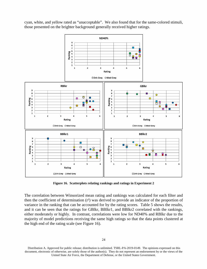
3.2.2 Rating As in Experiment 1, the model predictions for the nine stimuli were rated with the same anchors: 1= “Completely Unacceptable” to 6 = “Completely Acceptable”. Scatterplots between the Rankings and Ratings for each filter are shown in Figure 16. Squares are for stimuli presented on the dark grey background and circles are for stimuli presented on the medium grey background. We can see from Figure 16, that subjects rated all of the stimuli with the ND40% filter between 5 & 6 and all but one stimulus with the RBlkr filter between 4 & 6. While most stimuli received positive ratings (greater than or equal to 3.5) for GBlkr and BBlk1 several did not, including green for GBlkr and blue for BBlkr1. For BBlkr2, stimulus ratings spanned the whole range with blue,
24
Distribution A. Approved for public release; distribution is unlimited. TSRL-PA-2019-0149. The opinions expressed on this document, electronic of otherwise, are solely those of the author(s). They do not represent an endorsement by or the views of the
United State Air Force, the Department of Defense, or the United States Government.
cyan, white, and yellow rated as “unacceptable”. We also found that for the same-colored stimuli, those presented on the brighter background generally received higher ratings.
Figure 16. Scatterplots relating rankings and ratings in Experiment 2
The correlation between Winsorized mean rating and rankings was calculated for each filter and then the coefficient of determination (r²) was derived to provide an indicator of the proportion of variance in the ranking that can be accounted for by the rating scores. Table 5 shows the results, and it can be seen that the ratings for GBlkr, BBlkr1, and BBlkr2 correlated with the rankings, either moderately or highly. In contrast, correlations were low for ND40% and RBlkr due to the majority of model predictions receiving the same high ratings so that the data points clustered at the high end of the rating scale (see Figure 16).

25
Distribution A. Approved for public release; distribution is unlimited. TSRL-PA-2019-0149. The opinions expressed on this document, electronic of otherwise, are solely those of the author(s). They do not represent an endorsement by or the views of the
United State Air Force, the Department of Defense, or the United States Government.
Table 5. Proportion of variance accounted for (r²) between the ratings and rankings of the predictions in Experiment 2
ND40 RBlkr GBlkr BBlkr1 BBlkr2 Mean Medium 0.339 0.008 0.524 0.717 0.759 0.469 Dark 0.007 0.000 0.524 0.612 0.796 0.483 Mean 0.173 0.004 0.524 0.664 0.777 0.492
3.2.3 Color Matching The differences between the subjects’ XYZ matches and the model XYZ predictions were computed for each stimulus color for each filter for each subject. To equate lightness and chromaticity differences from predictions, the d E*uv differences were computed from the XYZ differences. These dE*uv were decomposed into dL* (lightness) and du*v*(chromaticity) measures.
To test for differences between filters, a 5 × 9 × 2 repeated measures ANOVA was computed for the dE*uv, dL*, and du*v* data. The factors were filter (five levels), stimulus color (nine levels), and background luminance (two levels). Since sphericity was a concern in some cases, we used the Greenhouse-Geisser epsilon-adjusted degrees of freedom to protect alpha. Table 6 summarizes the results of the analysis.
Table 6. Results of the ANOVA for the Matching Data in Experiment 2
Note: For F values, ** = p < .001; * = p < .01; + = p < .05
From Table 6, it can be seen that for d E*uv, there was a main effect of filter. When predictions between ND40% and each of the LEP were compared, we found no difference for the RBblkr but that predictions for the other three LEP were all worse than ND40%. For d E*uv, there was also a significant main effect of stimulus color and a significant interaction between filter and stimulus color. This indicates that the size of dE*uv was not the same for all colors and also that the pattern of differences was not the same for all LEP. We also found the effect of background to be significant due to poorer predictions on the dark compared to the medium grey background. The
dE*uv d L* d u*v*Factor df F df F df F
Filter 2.5, 12.6 22.282** 1.8, 8.9 2.993 2.7, 13.3 20.747**ND v RBlkr 1, 5 < 1 1, 5 < 1 1, 5 < 1ND v GBlkr 1, 5 26.512* 1, 5 3.275 1, 5 26.364*
ND v BBlkr1 1, 5 10.186+ 1, 5 3.551 1, 5 9.715+ND v BBlkr2 1, 5 29.59* 1, 5 4.994 1, 5 28.123*
Stim Color 1.7, 8.6 10.157* 1.3, 6.4 9.415+ 2.1, 10.3 9.263**Background 1,5 25.299* 1, 5 5.264 1,5 24.17*Filter x Stim Color 3.2, 16.0 5.718* 3.1, 15.6 2.245 3.2, 16.2 5.754*Filter x Background 1.3, 6.6 1.874 2.2, 11.1 1.845 1.4, 6.9 1.759
26
Distribution A. Approved for public release; distribution is unlimited. TSRL-PA-2019-0149. The opinions expressed on this document, electronic of otherwise, are solely those of the author(s). They do not represent an endorsement by or the views of the
United State Air Force, the Department of Defense, or the United States Government.
effect of background did not enter into any interaction indicating that the background effect was similar across LEP and stimulus color.
For d L*, we found the effect of filter failed to reach statistical significance (p= .105) and neither did any of the comparisons between the LEP and the ND40% filter. However, the main effect of stimulus color was significant and due primarily to predictions for the two brightest stimuli (white and yellow) being consistently the worst across filters. Neither the main effect of background nor any interaction reached statistical significance.
For chromaticity differences (d u*v*) we found a number of significant effects. First, there was a main effect of filter indicating that the magnitude of the overall chromaticity differences was not the same for all filters. Also the accuracy of predictions for the ND40% was better than all of the LEP except the RBlkr. The main effect of stimulus color was significant; as was the interaction between filter and stimulus color. These results suggest first that the magnitude of the chromaticity differences was not constant across colors, second that the pattern of differences was not the same across LEP. Unlike the lightness difference metric, we found a significant background effect for chromaticity differences and that it was the result of poorer predictions for stimuli presented against the darker background. Background, however, did not enter into any interaction.
In summary, the accuracy of predictions for the RBlkr were no worse from those for ND40%. The CIECAM02 model predicted the subject matches for RBlkr just as well as for ND40%. The E*uv predictions for the other three color filters were worse than for ND40% but the inaccuracies were not due to d L*. Instead, they were due to chromaticity changes (d u*v*) not being as well accounted for by the model as they were for the RBlkr and ND40%. All of the difference metrics varied in size across stimulus color and the patterns of the size of differences with color were not the same across LEP. Finally, predictions of overall appearance and chromaticity were worse for all filters on the dark background.
As we saw from Table 6, the interaction between filter and stimulus color was significant for the d E*uv and d u*v* measures. This interaction and the main effect of background are explored for RBlkr and BBlkr1filters in Figure 17. Similar plots for all the filters can be found in Appendix B. Although there was no filter effect for dL* those data are included to illustrate that that there were some lightness prediction differences as a function of stimulus color. For the RBlkr filter, all the predictions were very accurate and differences were comparable in size to those obtained with ND40% and reflect the lack of a significant difference in model predictions for the two filters. For the GBlkr filter, predictions were poorer for the green and yellow stimuli, and dark grey background predictions were worse than medium grey background predictions for most colors. Figure 17 also illustrates that the larger contributor to color appearance differences were chromaticity differences.

27
Distribution A. Approved for public release; distribution is unlimited. TSRL-PA-2019-0149. The opinions expressed on this document, electronic of otherwise, are solely those of the author(s). They do not represent an endorsement by or the views of the
United State Air Force, the Department of Defense, or the United States Government.
Figure 17. The effects of stimulus color and background (medium or dark) on d E*uv (top panel), d L* (middle panel), and d u*v* (bottom panel) for the RBlkr and BBlkr1 filters.
Error bars ± 1 SE
As in Experiment 1, the big differences between filters were based on d u*v*. To provide a strong test of the CIECAM02 model, some of the filters were chosen to produce extreme shifts in u’v’ space. Those shifts in u’v’ space are shown in Figure 18. The unfiltered stimuli (diamonds) are located across the Adobe RGB gamut. Many of the filtered stimuli (tail of the arrows) lie outside the gamut and could not be presented on the monitor. Except for the ND40 filter (which produced filtering effects in brightness rather than chromaticity) the adapted predictions (tip of the arrows) are closer to the original, unfiltered stimuli. Figure 18 shows both the effects of filtering and the recovery effects of chromatic adaptation accounted for by the CIECAM02 adaptation transform.
Figure 19 shows the subjects’ matches relative to the Fairchild emissive mode predictions. Again, the filtered and adapted stimuli are the arrow tips. The squares are the subject matches for stimuli
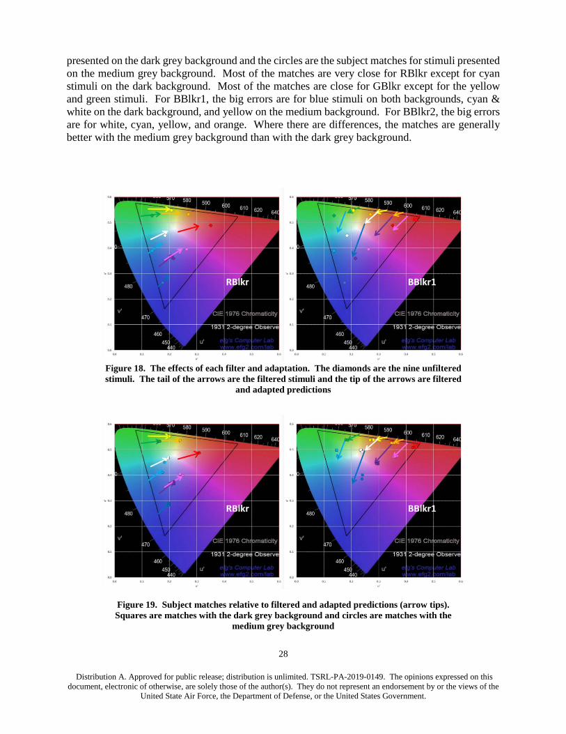
28
Distribution A. Approved for public release; distribution is unlimited. TSRL-PA-2019-0149. The opinions expressed on this document, electronic of otherwise, are solely those of the author(s). They do not represent an endorsement by or the views of the
United State Air Force, the Department of Defense, or the United States Government.
presented on the dark grey background and the circles are the subject matches for stimuli presented on the medium grey background. Most of the matches are very close for RBlkr except for cyan stimuli on the dark background. Most of the matches are close for GBlkr except for the yellow and green stimuli. For BBlkr1, the big errors are for blue stimuli on both backgrounds, cyan & white on the dark background, and yellow on the medium background. For BBlkr2, the big errors are for white, cyan, yellow, and orange. Where there are differences, the matches are generally better with the medium grey background than with the dark grey background.
Figure 18. The effects of each filter and adaptation. The diamonds are the nine unfiltered stimuli. The tail of the arrows are the filtered stimuli and the tip of the arrows are filtered
and adapted predictions
Figure 19. Subject matches relative to filtered and adapted predictions (arrow tips). Squares are matches with the dark grey background and circles are matches with the
medium grey background
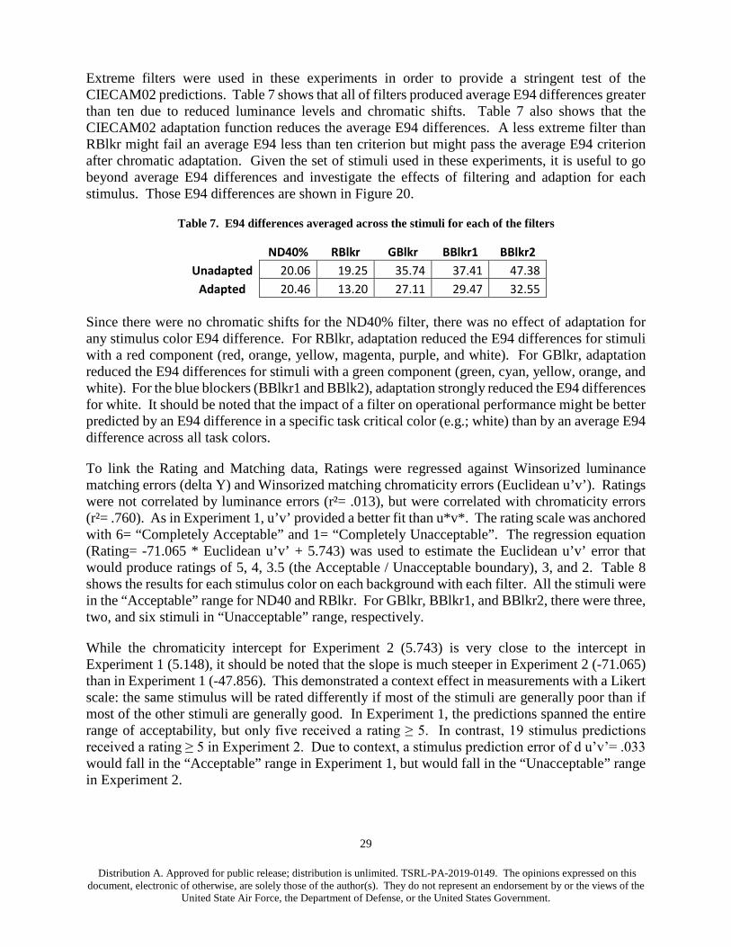
29
Distribution A. Approved for public release; distribution is unlimited. TSRL-PA-2019-0149. The opinions expressed on this document, electronic of otherwise, are solely those of the author(s). They do not represent an endorsement by or the views of the
United State Air Force, the Department of Defense, or the United States Government.
Extreme filters were used in these experiments in order to provide a stringent test of the CIECAM02 predictions. Table 7 shows that all of filters produced average E94 differences greater than ten due to reduced luminance levels and chromatic shifts. Table 7 also shows that the CIECAM02 adaptation function reduces the average E94 differences. A less extreme filter than RBlkr might fail an average E94 less than ten criterion but might pass the average E94 criterion after chromatic adaptation. Given the set of stimuli used in these experiments, it is useful to go beyond average E94 differences and investigate the effects of filtering and adaption for each stimulus. Those E94 differences are shown in Figure 20.
Table 7. E94 differences averaged across the stimuli for each of the filters
ND40% RBlkr GBlkr BBlkr1 BBlkr2 Unadapted 20.06 19.25 35.74 37.41 47.38
Adapted 20.46 13.20 27.11 29.47 32.55 Since there were no chromatic shifts for the ND40% filter, there was no effect of adaptation for any stimulus color E94 difference. For RBlkr, adaptation reduced the E94 differences for stimuli with a red component (red, orange, yellow, magenta, purple, and white). For GBlkr, adaptation reduced the E94 differences for stimuli with a green component (green, cyan, yellow, orange, and white). For the blue blockers (BBlkr1 and BBlk2), adaptation strongly reduced the E94 differences for white. It should be noted that the impact of a filter on operational performance might be better predicted by an E94 difference in a specific task critical color (e.g.; white) than by an average E94 difference across all task colors.
To link the Rating and Matching data, Ratings were regressed against Winsorized luminance matching errors (delta Y) and Winsorized matching chromaticity errors (Euclidean u’v’). Ratings were not correlated by luminance errors (r²= .013), but were correlated with chromaticity errors (r²= .760). As in Experiment 1, u’v’ provided a better fit than u*v*. The rating scale was anchored with 6= “Completely Acceptable” and 1= “Completely Unacceptable”. The regression equation (Rating= -71.065 * Euclidean u’v’ + 5.743) was used to estimate the Euclidean u’v’ error that would produce ratings of 5, 4, 3.5 (the Acceptable / Unacceptable boundary), 3, and 2. Table 8 shows the results for each stimulus color on each background with each filter. All the stimuli were in the “Acceptable” range for ND40 and RBlkr. For GBlkr, BBlkr1, and BBlkr2, there were three, two, and six stimuli in “Unacceptable” range, respectively.
While the chromaticity intercept for Experiment 2 (5.743) is very close to the intercept in Experiment 1 (5.148), it should be noted that the slope is much steeper in Experiment 2 (-71.065) than in Experiment 1 (-47.856). This demonstrated a context effect in measurements with a Likert scale: the same stimulus will be rated differently if most of the stimuli are generally poor than if most of the other stimuli are generally good. In Experiment 1, the predictions spanned the entire range of acceptability, but only five received a rating ≥ 5. In contrast, 19 stimulus predictions received a rating ≥ 5 in Experiment 2. Due to context, a stimulus prediction error of d u’v’= .033 would fall in the “Acceptable” range in Experiment 1, but would fall in the “Unacceptable” range in Experiment 2.
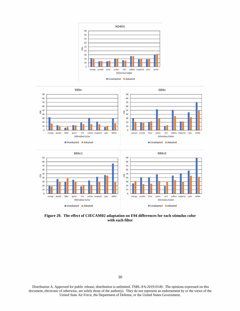
30
Distribution A. Approved for public release; distribution is unlimited. TSRL-PA-2019-0149. The opinions expressed on this document, electronic of otherwise, are solely those of the author(s). They do not represent an endorsement by or the views of the
United State Air Force, the Department of Defense, or the United States Government.
Figure 20. The effect of CIECAM02 adaptation on E94 differences for each stimulus color with each filter
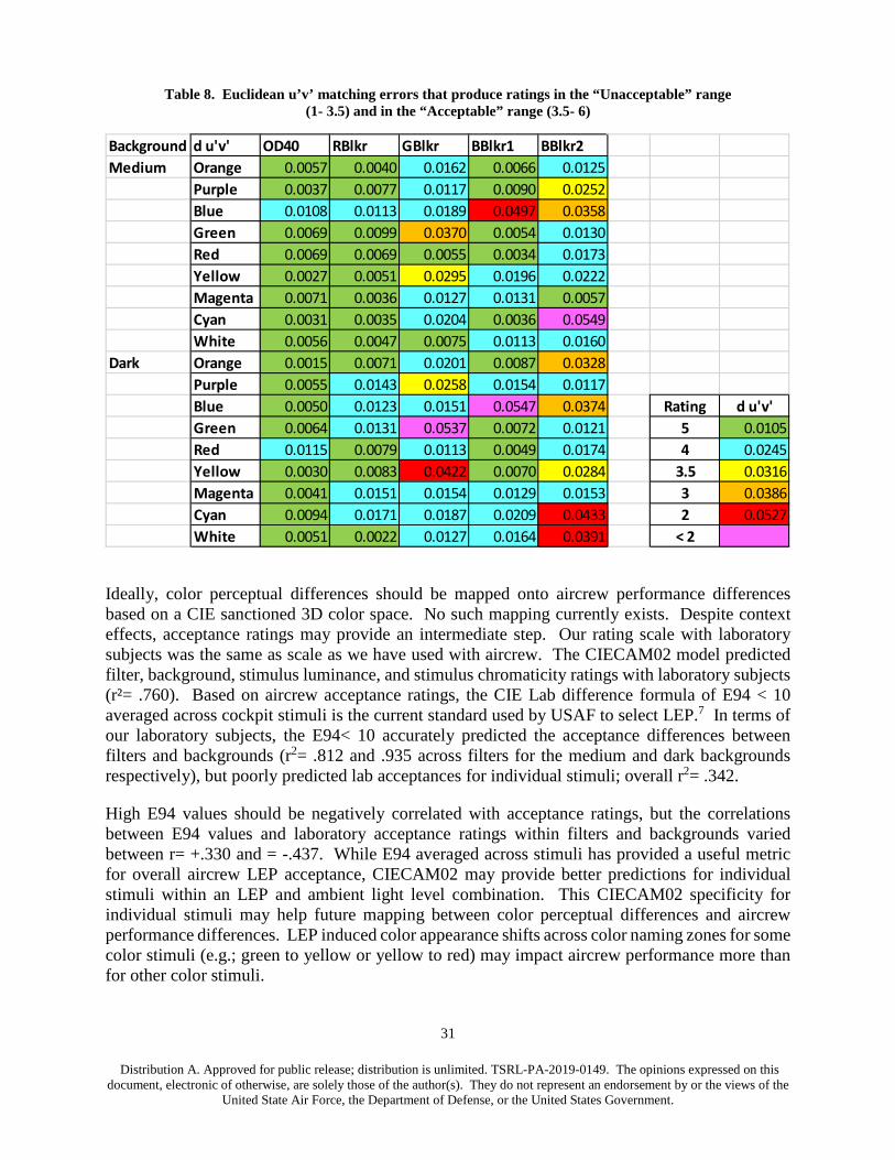
31
Distribution A. Approved for public release; distribution is unlimited. TSRL-PA-2019-0149. The opinions expressed on this document, electronic of otherwise, are solely those of the author(s). They do not represent an endorsement by or the views of the
United State Air Force, the Department of Defense, or the United States Government.
Table 8. Euclidean u’v’ matching errors that produce ratings in the “Unacceptable” range (1- 3.5) and in the “Acceptable” range (3.5- 6)
Ideally, color perceptual differences should be mapped onto aircrew performance differences based on a CIE sanctioned 3D color space. No such mapping currently exists. Despite context effects, acceptance ratings may provide an intermediate step. Our rating scale with laboratory subjects was the same as scale as we have used with aircrew. The CIECAM02 model predicted filter, background, stimulus luminance, and stimulus chromaticity ratings with laboratory subjects (r²= .760). Based on aircrew acceptance ratings, the CIE Lab difference formula of E94 < 10 averaged across cockpit stimuli is the current standard used by USAF to select LEP.7 In terms of our laboratory subjects, the E94< 10 accurately predicted the acceptance differences between filters and backgrounds (r2= .812 and .935 across filters for the medium and dark backgrounds respectively), but poorly predicted lab acceptances for individual stimuli; overall r2= .342.
High E94 values should be negatively correlated with acceptance ratings, but the correlations between E94 values and laboratory acceptance ratings within filters and backgrounds varied between r= +.330 and = -.437. While E94 averaged across stimuli has provided a useful metric for overall aircrew LEP acceptance, CIECAM02 may provide better predictions for individual stimuli within an LEP and ambient light level combination. This CIECAM02 specificity for individual stimuli may help future mapping between color perceptual differences and aircrew performance differences. LEP induced color appearance shifts across color naming zones for some color stimuli (e.g.; green to yellow or yellow to red) may impact aircrew performance more than for other color stimuli.
Background d u'v' OD40 RBlkr GBlkr BBlkr1 BBlkr2Medium Orange 0.0057 0.0040 0.0162 0.0066 0.0125
Purple 0.0037 0.0077 0.0117 0.0090 0.0252Blue 0.0108 0.0113 0.0189 0.0497 0.0358Green 0.0069 0.0099 0.0370 0.0054 0.0130Red 0.0069 0.0069 0.0055 0.0034 0.0173Yellow 0.0027 0.0051 0.0295 0.0196 0.0222Magenta 0.0071 0.0036 0.0127 0.0131 0.0057Cyan 0.0031 0.0035 0.0204 0.0036 0.0549White 0.0056 0.0047 0.0075 0.0113 0.0160
Dark Orange 0.0015 0.0071 0.0201 0.0087 0.0328Purple 0.0055 0.0143 0.0258 0.0154 0.0117Blue 0.0050 0.0123 0.0151 0.0547 0.0374 Rating d u'v'Green 0.0064 0.0131 0.0537 0.0072 0.0121 5 0.0105Red 0.0115 0.0079 0.0113 0.0049 0.0174 4 0.0245Yellow 0.0030 0.0083 0.0422 0.0070 0.0284 3.5 0.0316Magenta 0.0041 0.0151 0.0154 0.0129 0.0153 3 0.0386Cyan 0.0094 0.0171 0.0187 0.0209 0.0433 2 0.0527White 0.0051 0.0022 0.0127 0.0164 0.0391 < 2

32
Distribution A. Approved for public release; distribution is unlimited. TSRL-PA-2019-0149. The opinions expressed on this document, electronic of otherwise, are solely those of the author(s). They do not represent an endorsement by or the views of the
United State Air Force, the Department of Defense, or the United States Government.
4 CONCLUSIONS In two experiments, we tested the capability of CIECAM02 to predict the adjustments made by the visual system to preserve the appearance of colored stimuli viewed through a neutral filter and four colored filters. At the same time, we evaluated the accuracy of a software implementation of the model.6 In order to provide a sensitive test of CIECAM02, the filters were selected to be extreme relative to aircrew needs. The 40% transmittance of the ND40% filter would be too dark for most aircrew nighttime operations but was needed to control for any effect of the PLT of the colored filters (which ranged between 47% and 56% PLT). According to a study of A-10 pilots27, nighttime LEP “above a threshold value of 50% are likely to be accepted by aircrew”. Further, “For filters with transmission below 50%, results suggest pilots would knowingly expose themselves to real laser threats nearly a quarter of the time versus the tradeoff in perceived performance degradation”. The colored filters used were also selected because they were LEP and they blocked operationally relevant regions of the visible spectrum to varying degrees. To obtain a general indication of the effects of the filters on color vision we had subjects complete the Lanthony 40 color vision test with each filter. For the Lanthony test, we found the RBlkr and GBlkr filters had little effect on performance on the test and produced error scores well inside the normal range and no different than the score obtained with the neutral control filter. In contrast both of the blue-blockers produced error scores significantly higher than the neutral control filter, with BBlkr2 producing a score that fell outside the normal range. We attribute the poorer performance with the blue-blockers to their greater restriction of the spectral range of light reaching the photoreceptors. Both filters significantly reduce the amount of light available to the S- and M-cones. We found this restriction resulted in large shifts in the location of the caps in color space such that they lost their circular organization (see Figure 6) and became more linearly arranged and in a more restricted region of color space. This resulted in the caps having limited variation in hue, which in turn led to difficulty arranging them in an orderly progression of changing hue. In contrast the color shifts caused by the RBlkr and GBlkr, while large, did not completely disrupt the circular organization of the caps and we believe this allowed subjects to make fairly orderly arrangements of the caps by hue. To evaluate the CAM02, the experimental approach we used was a haploscopic view where subjects compared a stimulus viewed though a neutral or colored filter to a stimulus whose appearance through the filter is predicted by the CIECAM02 model. Subjects viewed nine stimuli in an array and rank ordered them from best to worst prediction. They then rated the predictions for accuracy on a six-point scale after which they adjusted the color and luminance of the predicted stimuli to achieve the closest match to the actual stimuli. If the model predictions were accurate, adjustments would be unnecessary or small, while large errors in prediction would require larger adjustments to achieve a match with the actual stimulus. In Experiment 1, we tested model predictions for colors that occur because of objects reflecting various amounts of the visible spectrum of a light source that illuminates them. We selected a subset of nine colors from the Macbeth color checker and determined their spectral content from the spectral content of the D65 light source illuminating them and the spectral reflectance properties of each object. From this, we calculated the CIE tristimulus values, X, Y, and Z for each color and those values served as the stimulus information put into the model.
33
Distribution A. Approved for public release; distribution is unlimited. TSRL-PA-2019-0149. The opinions expressed on this document, electronic of otherwise, are solely those of the author(s). They do not represent an endorsement by or the views of the
United State Air Force, the Department of Defense, or the United States Government.
Although Experiment 1 results initially appeared to be reasonable, subsequent review of the source code for the emissive mode revealed that there were order of operation errors present in the forward and inverse transforms. We addressed these problems in a second experiment, using the Fairchild Excel spreadsheet26 to set input model parameters for the emissive mode of computer presented stimuli. The same nine unfiltered stimuli from Experiment 1 were used in Experiment 2. The filtered stimuli differed, because filtering was based on the XYZ contrast matching functions in Experiment 1 and was based on the EIZO RGB channels in Experiment 2. For Experiment 2, the filtered stimulus values were entered into Fairchild’s implementation of the CAM02 calculations for the forward and inverse transform and the results were converted on the back end to the RGB values of the predicted stimuli displayed on our monitor. In Experiment 2, we recruited experienced observers and were able to make background a repeated measure. As a result, with six subjects, we had sufficient power for hypothesis testing: whether model predictions were different than subject matches. Anticipated future experiments are still inferential and address the same question, do subject matches correspond to model predictions? Sample size for those steps depends on both power and technique. We anticipate again using haploscopic matching but to reduce the number of filters to four by eliminating the very extreme BBlkr2. If so, a sample size of eight would provide sufficient power in a repeated-measures design for hypothesis testing, while allowing for counter-balancing of sessions across the four filters. Adding additional subjects would likely reduce variance in the data and result in smaller differences between subject matches and model predictions being statistically significant but this would not necessarily improve our ability to test hypotheses related to what factors are responsible for any differences. We found that the emissive mode made surprisingly accurate predictions given the extreme filters tested. By accurate, we mean, considering the whole set of filters, du’v’ matching errors of ≤0.0316, which corresponds to the boundary between acceptable and unacceptable ratings determined from our regression analysis. For the RBlkr, which reduced light available to the L-cones by 49%, predictions were just as accurate as those made with the neutral filter. Further, all predictions were rated in the acceptable range. The GBlkr, which filtered the middle of the spectrum, reduced the light available to the M-cones by nearly 70% and S-cones by 80% yielded predictions for the green and yellow stimuli that required large adjustments by the subject to match the actual stimuli and moderate adjustments to match orange and magenta. Interestingly we found that only the green prediction was rated as unacceptable. The two blue blockers were the most extreme filters with respect to S-cones with BBlkr1 reducing the light available to S-cones by 94% and BBlkr2 by 99.6%. Surprisingly, the model predicted color appearance quite well for BBlkr1 and only blue stimuli predictions were rated in the unacceptable range and only blue stimuli produced large matching errors. For BBlkr2, the predictions for yellow, cyan and white produced large matching errors and orange moderate errors. We also found the BBlkr2 yielded more unacceptable ratings for model predictions with three of nine predictions rated unacceptable on the medium grey background and five of nine on the dark grey background. This may have been the result of BBlkr2 also reducing light available to M-cones by a larger amount than BBlkr1.
34
Distribution A. Approved for public release; distribution is unlimited. TSRL-PA-2019-0149. The opinions expressed on this document, electronic of otherwise, are solely those of the author(s). They do not represent an endorsement by or the views of the
United State Air Force, the Department of Defense, or the United States Government.
For the GBlkr and BBlkr1 filters, the predictions were almost all rated as acceptable even though the matching results and the boundary between acceptable and unacceptable based on regression analysis suggest that some of these acceptable predictions were inaccurate. We suspect this occurred because the hue of the prediction was similar enough to that of the actual stimulus that subjects considered them to be in the same color name category. For example, for the GBlkr, the yellow prediction (tip of arrow) falls in a region of color space associated with orange hues and the subject match which, although shifted toward longer wavelengths still falls into the region associate with orange hues. In contrast the green prediction which was judged inaccurate, falls into the area of color space associated with greens and yellowish-greens, however, the actual stimulus that subjects matched falls into the zone associated with yellows. Color zone analysis, where match prediction are related to color zones in color space may be an important direction for future research in relating acceptability of color shifts caused by LEP.28 Generally, ratings were lower and matching predictions were worse with the Dark Grey background than with the Medium Grey background. CIECAM02 has viewing condition parameters (F, c, Nc, La, and Yb) and a degree of adaptation parameter (D). In the emissive mode predictions Experiment 2, the standard F, C, and Nc parameters were adopted for a “Dark” environment. The prototypical “Dark” is viewing slides (Y= 150 cd·m-²) in a dark room.29 The monitor conditions for this study were much darker. The La and Yb parameters were set to 20 (standard used in a grey world assumption with a maximum Y= 100 cd·m-²) compared to 30 for slides presented at 150 cd·m². The dark and medium grey backgrounds in this study were 9.4 and 36.0 cd·m-², respectively. The degree of adaptation (D) might have been lower in our lab setup than the standard assumed with typical computer presentations. One of the challenges that we faced before conducting this study was how to determine the initial model parameters to optimize the appearance of model predictions for our viewing situation. As noted previously, the solution was to adopt standard settings for a dark background and as a compromise for the two background conditions (9.4 and 36.0 cd·m-²) set the background and surround to 20 cd·m-². Other parameters were set according to CIE recommendations or calculated depending on the mode. Ideas for conducting future studies include dynamic feedback to allow subjects the ability to adjust a selection of viewing parameters in the haploscopic viewing mode. It might also be possible to display the original model predictions and the predictions as parameters are changed on one side to provide subjects with an appreciation for changes associated with the individual parameters. This capability would allow rapid determination of the effects of changing parameter settings on model predictions and may allow us to better optimize the color appearance of the model predictions for viewing conditions that are not standard. It would also allow us to extend CIECAM02 to higher photopic levels and also to lower mesopic levels that typify the cockpit environment during daytime and nighttime operations.
Extending the CIECAM02 model into the mesopic range is currently an active research area.21,30,31 The upper bound of the mesopic range is estimated to be about 3-5 cd·m-². Our blue and purple stimuli were in the mesopic range with all of our filters (range 1.5-4.2 cd·m-²). The dark background was also in that ballpark (range 2.7-5.8 cd·m-²). It is likely that some of our matches were influenced by rod- cone interactions. As noted above, we will adjust model parameters to see if we can improve the predictions of Experiment 2. In addition, we will explore the effects of stimulus size and unrelated colors in a follow up experiment. Recent research21,31 indicates that
35
Distribution A. Approved for public release; distribution is unlimited. TSRL-PA-2019-0149. The opinions expressed on this document, electronic of otherwise, are solely those of the author(s). They do not represent an endorsement by or the views of the
United State Air Force, the Department of Defense, or the United States Government.
the appearance of unrelated colors (landing lights at night are an example) needs to be modeled differently than related colors (moving map displays and natural scenes are examples) in the mesopic range.
While the CIECAM02 model is fairly accurate at predicting the effects of wearing LEP, the results also show that the visual system does not fully recover via adaptation to the light filtering effects. This is evident in comparing the location of the original unfiltered stimuli to the location of the model predictions (or subject matches) in color space. The gap between the two is most apparent for BBlkr2. The importance of this gap is that it represents the differences between unfiltered and filtered adapted stimuli on which, if they were representative of a cockpit display, pilots would base judgements of acceptability of the appearance changes caused by an LEP. Presently, we do not have a very good link between color differences and acceptability of changes caused by colored filters (although we have found a strong association between differences and color identification performance).28 However, the CIECAM02 model might be effectively used to gather such information by allowing subjects to make acceptability judgements of model predictions of what colors on a display, for example, will look like through LEP, in comparison to unfiltered original stimuli.
Also, as a next step towards a more deliberate verification and validation of the model, we will we investigate whether we can improve the model predictions compared to the subject matches through adjustment of the model input parameters. For this study the input parameters were selected based on our assumptions for our uncommon viewing situation, for which standards do not exist. While the results we obtained were very good, they may have been better had we based the input parameters on different assumptions. Our aim would be to perform a systematic adjustment of the input parameters to obtain the best fit of the model predictions to the experimental data, and then to reconsider our assumptions in the context of these optimal input parameters.
In summary, based upon our initial laboratory evaluation, we conclude that the CIECAM02 model is a valid model for predicting the effects of adaptation on the appearance of colored stimuli while wearing LEP. A potential application of this research includes the development of stand-alone software that uses complex images indicative of operational displays for familiarizing pilots with changes in the appearance of colored stimuli caused by LEP, as well as determining if color shifts with prototype LEP are acceptable to aircrew. The program could also be used by LEP filter and cockpit display developers to predict effects of new filter designs and to evaluate compatibility of new filters with color displays and for adjusting the color palette of a monitor to optimize visibility. For maximum relevance, the display should be a color display common to Air Force cockpits. We are currently investigating how to accomplish integrating the model with such a device. The program may require the use of a lower level programming language, such as Python or C++ to provide a more functional framework, increase computational efficiency, and thereby improve the speed with which simulations are generated.
36
Distribution A. Approved for public release; distribution is unlimited. TSRL-PA-2019-0149. The opinions expressed on this document, electronic of otherwise, are solely those of the author(s). They do not represent an endorsement by or the views of the
United State Air Force, the Department of Defense, or the United States Government.
REFERENCES
1. Kuyk, T. K., Engler, S., Garcia, P. V., Smith, P. A., Novar, B. J., & Putnam, C. M. (2016). Nighttime Visor Laser Eye Protection: Visual Function Testing. Technical Report AFRL-RH-FS-TR-2016-0013, Air Force Research Laboratory, Fort Sam Houston, TX 78234.
2. Novar, B. J., Beilby, J. P., Zucker, A., Constable, W., Chung, J., Engler, S., Kuyk, T. K., & Smith, P. A. (2015). Daytime Visor Laser Eye Protection: Ground and Flight Testing. Technical Report AFRL-RH-FS-TR-2015-0018, Air Force Research Laboratory, Fort Sam Houston, TX 78234.
3. Putnam, C. M., Novar, B. J., Goettl, B. P., Kuyk, T. K., Smith, P. A., & Engler, S. (2017). Nighttime Visor Laser Eye Protection: Ground and Flight Testing. Technical Report AFRL-RH-FS-TR-2017-0007, Air Force Research Laboratory, Fort Sam Houston, TX 78234.
4. Lucassen, M. P. (2001). Visualization of the effects of laser eye protection filters on colour perception. TM-01-A059, TNO Human Factors, Soesterberg, The Netherlands.
5. Brockmeier, W. R., Guevara, M. A., Kuyk, T. K., Morin, A. O., & Novar, B. J. (2015). Simulating the visual effects of wearing colored filters. Technical Report AFRL-RH-FS-TR-2015-0066, Air Force Research Laboratory, Fort Sam Houston, TX 78234.
6. Williamson, C. A., & Boontanrart, M. Y. (2016). Simulating the impact of laser eye protection on color vision. Journal of Laser Applications, 28, 012010.
7. ASC/WNUV. (2010). Performance Specification for Block 2 Laser Eye Protection (ALEP) Night Only Variant. ASC/WNUV-10-ALEPM-PS001 Rev D, Department of the Air Force, Air Systems Command, Wright Patterson AFB, OH 45433.
8. Air Force Life Cycle Management Center - Human Systems Division (AFLCMC/WNU). (2018). Product Specification for Aircrew Laser Eye Protection (ALEP) Block 3 Daytime Spectacles. Department of the Air Force, Air Force Material Command,. Available at: https://www.fbo.gov/index?s=opportunity&mode=form&id=558d51d6751f0919f38ad2f795b4301c&tab=core&_cview=1, last accessed on 5 Dec 2018.
9. USAF Warfare Center. (2012). Aircrew Laser Eye Protection Block 2 Force Development Evaluation - Final Report. ACC PROJECT 08-115A, USAF Warfare Center, Nellis Air Force Base, NV 89191.
10. Fairchild, M. D. (2013). Color appearance models (3rd ed.). Chichester, West Sussex, U.K: John Wiley & Sons, Ltd.
11. International Commission on Illumination (CIE). (2004). A color appearance model for color management systems: CIECAM02. Technical Report Publication 159, CIE TC 8-01, Vienna, Austria.

37
Distribution A. Approved for public release; distribution is unlimited. TSRL-PA-2019-0149. The opinions expressed on this document, electronic of otherwise, are solely those of the author(s). They do not represent an endorsement by or the views of the
United State Air Force, the Department of Defense, or the United States Government.
12. von Kries, J. (1902). Chromatic adaptation. Festscrift der Albrecht-Ludwig-Universtat, (Fribourg). [trans. D.L. MacAdam, Sources of Color Science, MIT Press, Cambridge (1970)].
13. Lucassen, M. P., & Walraven, J. (1993). Quantifying color constancy: evidence for nonlinear processing of cone-specific contrast. Vision research, 33, 739-757.
14. Moroney, M. D., Fairchild, M. D., Hunt, R. W. G., Li, C. J., Luo, M. R., & Newman, T. (2002). The CIECAM02 color appearance model. Proceedings of the IS&T/SID 10th Color Imaging Conference, Scottsdale, AZ.
15. Fairchild, M. D. (1995). Testing color appearance models: Guidelines for coordinated research. Color Research & Application, 20, 262-267.
16. Breneman, E. J. (1987). Corresponding chromaticities for different states of adaptation to complex visual fields. Journal of the Optical Society of America. A, Optics and image science, 4, 1115-1129.
17. Macadam, D. L. (1956). Chromatic adaptation. J Opt Soc Am, 46, 500-513.
18. Macadam, D. L. (1961). A nonlinear hypothesis for chromatic adaptation. Vision research, 1, 9-41.
19. Brainard, D. H., & Wandell, B. A. (1991). A bilinear model of the illuminant's effect on color appearance. In M. S. Landy & J. A. Movshon (Eds.)Computational models of visual processing. Cambridge, MA: MIT Press.
20. Brainard, D. H., & Wandell, B. A. (1992). Asymmetric color matching: how color appearance depends on the illuminant. Journal of the Optical Society of America. A, Optics and image science, 9, 1433-1448.
21. Fu, C., Li, C., Cui, G., Luo, M. R., Hunt, R. W. G., & Pointer, M. R. (2011). An investigation of colour appearance for unrelated colours under photopic and mesopic vision. Color Research & Application, 37, 238-254.
22. Hunt, R. W. G., & Luo, M. R. (1994). Evaluation of a model of colour vision by magnitude scalings: Discussion of collected results. Color Research & Application, 19, 27-33.
23. Withouck, M., Smet, K. A., Ryckaert, W. R., Deconinck, G., & Hanselaer, P. (2014). Predicting the brightness of unrelated self-luminous stimuli. Optics express, 22, 16298-16309.
24. Fairchild, M. D., Pirrotta, M., & Kim, T. (1994). Successive‐ganzfeld haploscopic viewing technique for color‐appearance research. Color Research & Application, 19, 214-221.
25. Kuyk, T. K., Engler, S., Brockmeier, W. R., Kumru, S. S., & Mariano, N. (2013). The effects of daytime laser eye protection for fixed and rotary wing aircraft on visual function.
38
Distribution A. Approved for public release; distribution is unlimited. TSRL-PA-2019-0149. The opinions expressed on this document, electronic of otherwise, are solely those of the author(s). They do not represent an endorsement by or the views of the
United State Air Force, the Department of Defense, or the United States Government.
Technical Report AFRL-RH-FS-TR-2013-0024, Air Force Research Laboratory, Fort Sam Houston, TX 78234.
26. Fairchild, M. D. (2018). Colour Appearance Models - Example Calculations and Functions. Available at: http://rit-mcsl.org/fairchild/files/AppModEx.xls, last accessed on 17 Jan.
27. LaFrance, M., Kent, J. F., Foutch, B. K., Miller, M., & Kuyk, T. K. (2009). Light transmission requirements for nighttime laser eye protection: preliminary findings. Technical Report AFRL-HE-BR-TR-2009-0041, Air Force Research Laboratory, Brooks City Base, TX 78235.
28. Kuyk, T. K., Dykes, J. R., & LaFrance, M. (2013). Predicting color naming with laser eye protection. Technical Report AFRL-RH-BR-TR-2010-0054, Air Force Research Laboratory, Brooks City Base, TX, 78235.
29. Luo, M. R., & Li, C. (2013). CIECAM02 and Its Recent Developments. In C. Fernandez-Maloigne (Ed.)Advanced Color Image Processing and Analysis. New York, NY: Springer.
30. Dykes, J. R. (2009). Modeling mesopic vision based on measured photopic sensitivity. AFRL-HE-BR-TR-2009-0051, USAF Research Laboratory, Brooks City-Base TX 78235.
31. Wei, S. T., Luo, M. R., Xiao, K., & Pointer, M. R. (2017). A comprehensive model of colour appearance for related and unrelated colours of varying size viewed under mesopic to photopic conditions. Color Research & Application, 42, 239-304.
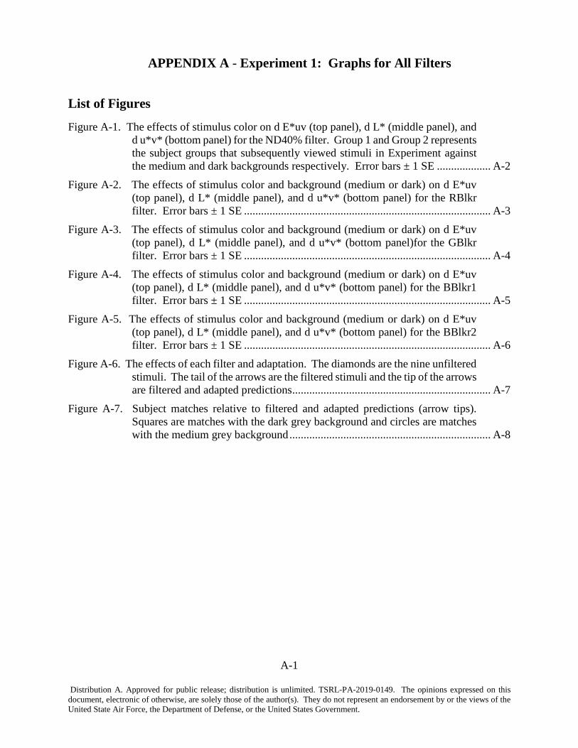
A-1
Distribution A. Approved for public release; distribution is unlimited. TSRL-PA-2019-0149. The opinions expressed on this document, electronic of otherwise, are solely those of the author(s). They do not represent an endorsement by or the views of the United State Air Force, the Department of Defense, or the United States Government.
APPENDIX A - Experiment 1: Graphs for All Filters
List of Figures
Figure A-1. The effects of stimulus color on d E*uv (top panel), d L* (middle panel), and d u*v* (bottom panel) for the ND40% filter. Group 1 and Group 2 represents the subject groups that subsequently viewed stimuli in Experiment against the medium and dark backgrounds respectively. Error bars ± 1 SE ................... A-2
Figure A-2. The effects of stimulus color and background (medium or dark) on d E*uv (top panel), d L* (middle panel), and d u*v* (bottom panel) for the RBlkr filter. Error bars ± 1 SE ....................................................................................... A-3
Figure A-3. The effects of stimulus color and background (medium or dark) on d E*uv (top panel), d L* (middle panel), and d u*v* (bottom panel)for the GBlkr filter. Error bars ± 1 SE ....................................................................................... A-4
Figure A-4. The effects of stimulus color and background (medium or dark) on d E*uv (top panel), d L* (middle panel), and d u*v* (bottom panel) for the BBlkr1 filter. Error bars ± 1 SE ....................................................................................... A-5
Figure A-5. The effects of stimulus color and background (medium or dark) on d E*uv (top panel), d L* (middle panel), and d u*v* (bottom panel) for the BBlkr2 filter. Error bars ± 1 SE ....................................................................................... A-6
Figure A-6. The effects of each filter and adaptation. The diamonds are the nine unfiltered stimuli. The tail of the arrows are the filtered stimuli and the tip of the arrows are filtered and adapted predictions ...................................................................... A-7
Figure A-7. Subject matches relative to filtered and adapted predictions (arrow tips). Squares are matches with the dark grey background and circles are matches with the medium grey background ....................................................................... A-8
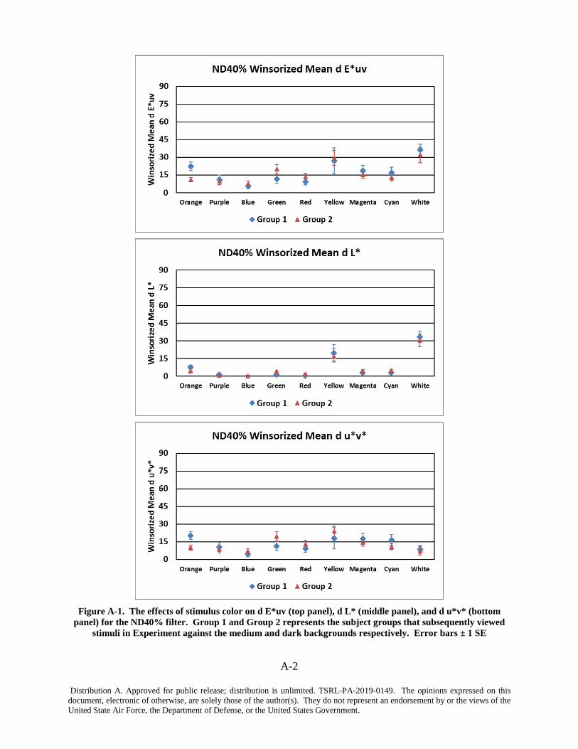
A-2
Distribution A. Approved for public release; distribution is unlimited. TSRL-PA-2019-0149. The opinions expressed on this document, electronic of otherwise, are solely those of the author(s). They do not represent an endorsement by or the views of the United State Air Force, the Department of Defense, or the United States Government.
Figure A-1. The effects of stimulus color on d E*uv (top panel), d L* (middle panel), and d u*v* (bottom
panel) for the ND40% filter. Group 1 and Group 2 represents the subject groups that subsequently viewed stimuli in Experiment against the medium and dark backgrounds respectively. Error bars ± 1 SE
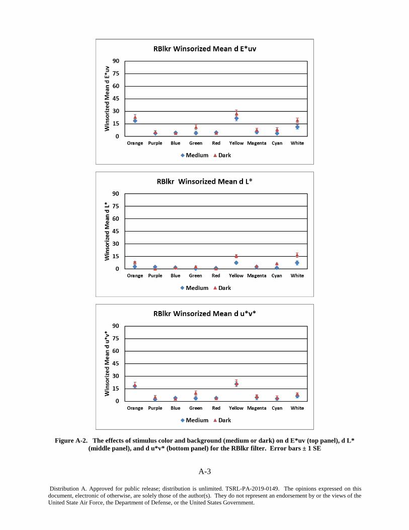
A-3
Distribution A. Approved for public release; distribution is unlimited. TSRL-PA-2019-0149. The opinions expressed on this document, electronic of otherwise, are solely those of the author(s). They do not represent an endorsement by or the views of the United State Air Force, the Department of Defense, or the United States Government.
Figure A-2. The effects of stimulus color and background (medium or dark) on d E*uv (top panel), d L* (middle panel), and d u*v* (bottom panel) for the RBlkr filter. Error bars ± 1 SE
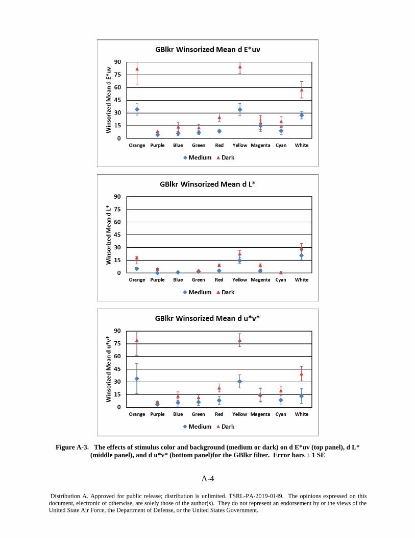
A-4
Distribution A. Approved for public release; distribution is unlimited. TSRL-PA-2019-0149. The opinions expressed on this document, electronic of otherwise, are solely those of the author(s). They do not represent an endorsement by or the views of the United State Air Force, the Department of Defense, or the United States Government.
Figure A-3. The effects of stimulus color and background (medium or dark) on d E*uv (top panel), d L* (middle panel), and d u*v* (bottom panel)for the GBlkr filter. Error bars ± 1 SE
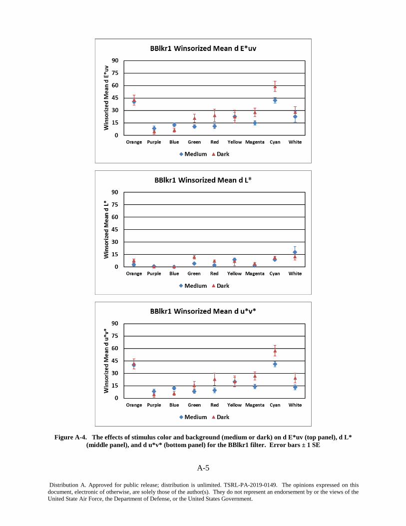
A-5
Distribution A. Approved for public release; distribution is unlimited. TSRL-PA-2019-0149. The opinions expressed on this document, electronic of otherwise, are solely those of the author(s). They do not represent an endorsement by or the views of the United State Air Force, the Department of Defense, or the United States Government.
Figure A-4. The effects of stimulus color and background (medium or dark) on d E*uv (top panel), d L* (middle panel), and d u*v* (bottom panel) for the BBlkr1 filter. Error bars ± 1 SE
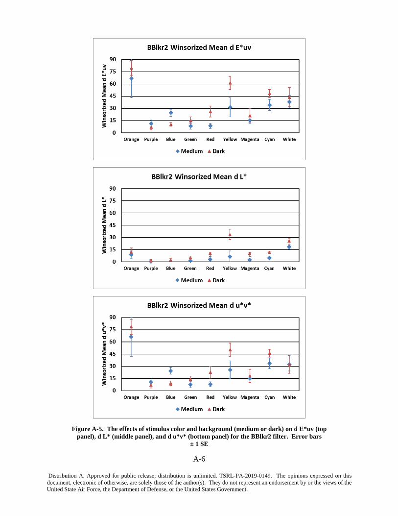
A-6
Distribution A. Approved for public release; distribution is unlimited. TSRL-PA-2019-0149. The opinions expressed on this document, electronic of otherwise, are solely those of the author(s). They do not represent an endorsement by or the views of the United State Air Force, the Department of Defense, or the United States Government.
Figure A-5. The effects of stimulus color and background (medium or dark) on d E*uv (top panel), d L* (middle panel), and d u*v* (bottom panel) for the BBlkr2 filter. Error bars
± 1 SE
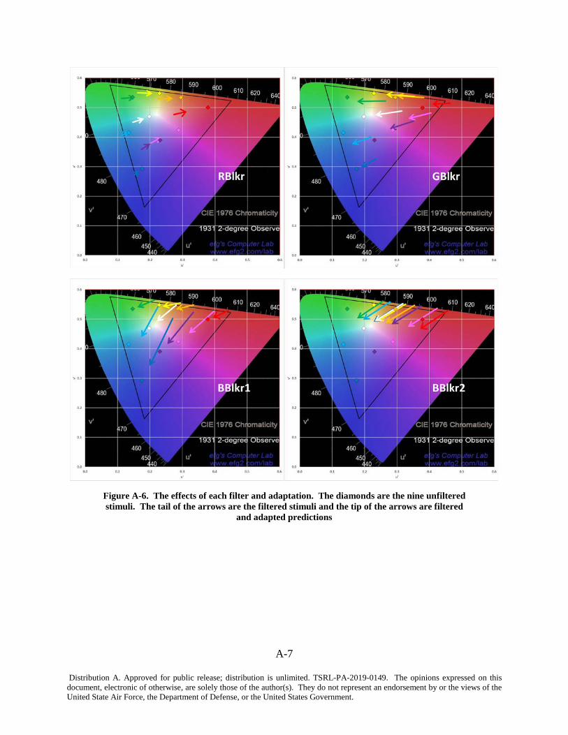
A-7
Distribution A. Approved for public release; distribution is unlimited. TSRL-PA-2019-0149. The opinions expressed on this document, electronic of otherwise, are solely those of the author(s). They do not represent an endorsement by or the views of the United State Air Force, the Department of Defense, or the United States Government.
Figure A-6. The effects of each filter and adaptation. The diamonds are the nine unfiltered stimuli. The tail of the arrows are the filtered stimuli and the tip of the arrows are filtered
and adapted predictions
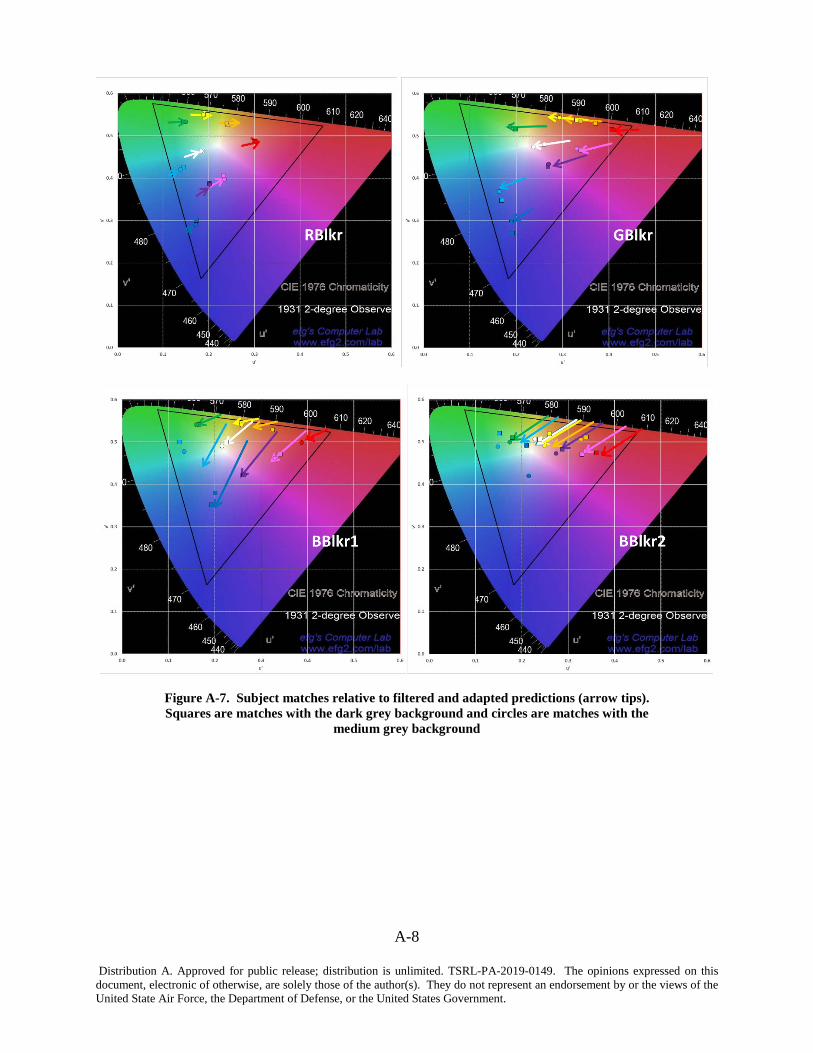
A-8
Distribution A. Approved for public release; distribution is unlimited. TSRL-PA-2019-0149. The opinions expressed on this document, electronic of otherwise, are solely those of the author(s). They do not represent an endorsement by or the views of the United State Air Force, the Department of Defense, or the United States Government.
Figure A-7. Subject matches relative to filtered and adapted predictions (arrow tips). Squares are matches with the dark grey background and circles are matches with the
medium grey background
B-1
Distribution A. Approved for public release; distribution is unlimited. TSRL-PA-2019-0149. The opinions expressed on this document, electronic of otherwise, are solely those of the author(s). They do not represent an endorsement by or the views of the United State Air Force, the Department of Defense, or the United States Government.
APPENDIX B - Experiment 2: Graphs for All Filters
List of Figures
Figure B-1. The effects of stimulus color and background (medium or dark) on d E*uv (top panel), d L* (middle panel), and d u*v* (bottom panel) for the ND40% filter. Error bars ± 1 SE ..........................................................................................B-2
Figure B-2. The effects of stimulus color and background (medium or dark) on d E*uv (top panel), d L* (middle panel), and d u*v* (bottom panel) for the RBlkr filter. Error bars ± 1 SE ..........................................................................................B-3
Figure B-3. The effects of stimulus color and background (medium or dark) on d E*uv (top panel), d L* (middle panel), and d u*v* (bottom panel) for the GBlkr filter. Error bars ± 1 SE ..........................................................................................B-4
Figure B-4. The effects of stimulus color and background (medium or dark) on d E*uv (top panel), d L* (middle panel), and d u*v* (bottom panel) for the BBlkr1 filter. Error bars ± 1 SE ..........................................................................................B-5
Figure B-5. The effects of stimulus color and background (medium or dark) on d E*uv (top panel), d L* (middle panel), and d u*v* (bottom panel) for the BBlkr2 filter. Error bars ± 1 SE .....................................................................................................B-6
Figure B-6. The effects of each filter and adaptation. The diamonds are the nine unfiltered stimuli. The tail of the arrows are the filtered stimuli and the tip of the arrows are filtered and adapted predictions ........................................................................B-7
Figure B-7. Subject matches relative to filtered and adapted predictions (arrow tips). Squares are matches with the dark grey background and circles are matches with the medium grey background .........................................................................B-8

B-2
Distribution A. Approved for public release; distribution is unlimited. TSRL-PA-2019-0149. The opinions expressed on this document, electronic of otherwise, are solely those of the author(s). They do not represent an endorsement by or the views of the United State Air Force, the Department of Defense, or the United States Government.
Figure B-1. The effects of stimulus color and background (medium or dark) on d E*uv (top panel), d L* (middle panel), and d u*v* (bottom panel) for the ND40% filter. Error bars
± 1 SE
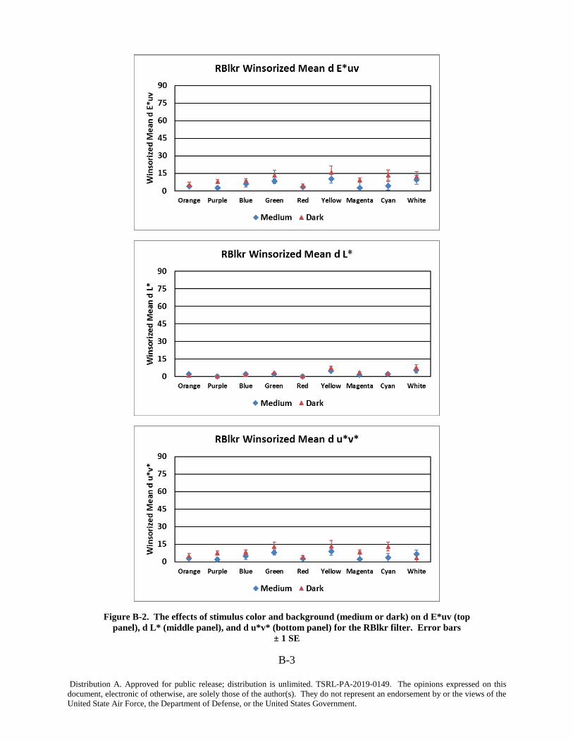
B-3
Distribution A. Approved for public release; distribution is unlimited. TSRL-PA-2019-0149. The opinions expressed on this document, electronic of otherwise, are solely those of the author(s). They do not represent an endorsement by or the views of the United State Air Force, the Department of Defense, or the United States Government.
Figure B-2. The effects of stimulus color and background (medium or dark) on d E*uv (top panel), d L* (middle panel), and d u*v* (bottom panel) for the RBlkr filter. Error bars
± 1 SE
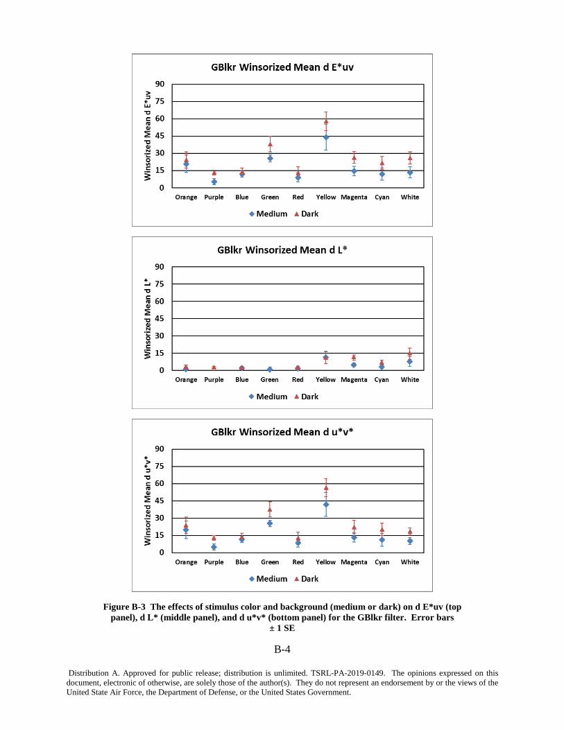
B-4
Distribution A. Approved for public release; distribution is unlimited. TSRL-PA-2019-0149. The opinions expressed on this document, electronic of otherwise, are solely those of the author(s). They do not represent an endorsement by or the views of the United State Air Force, the Department of Defense, or the United States Government.
Figure B-3 The effects of stimulus color and background (medium or dark) on d E*uv (top panel), d L* (middle panel), and d u*v* (bottom panel) for the GBlkr filter. Error bars
± 1 SE
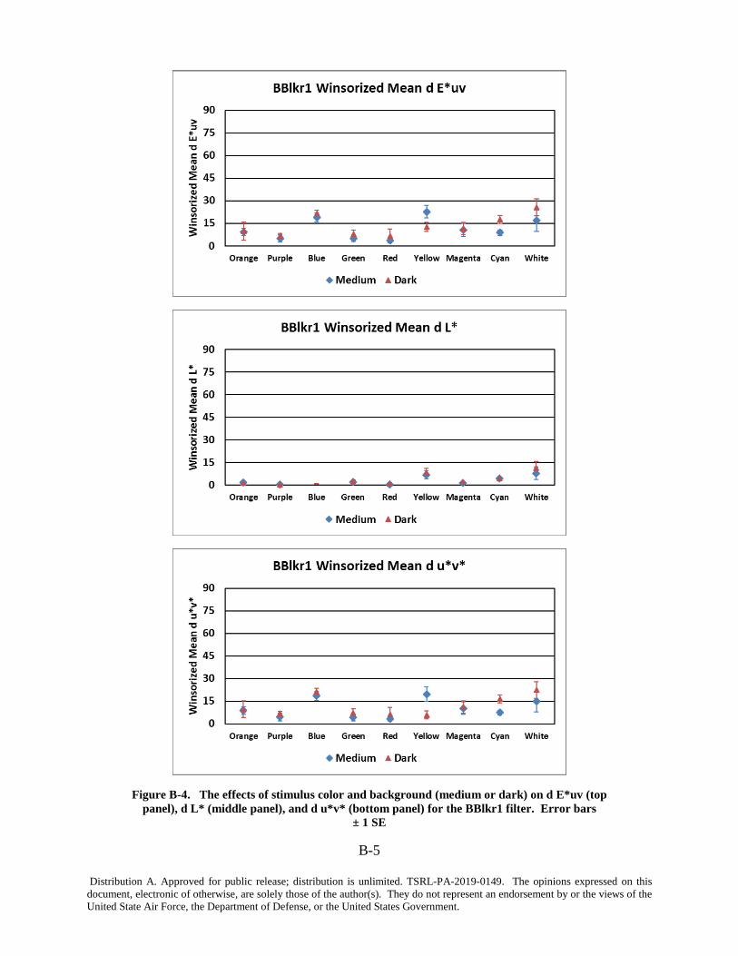
B-5
Distribution A. Approved for public release; distribution is unlimited. TSRL-PA-2019-0149. The opinions expressed on this document, electronic of otherwise, are solely those of the author(s). They do not represent an endorsement by or the views of the United State Air Force, the Department of Defense, or the United States Government.
Figure B-4. The effects of stimulus color and background (medium or dark) on d E*uv (top panel), d L* (middle panel), and d u*v* (bottom panel) for the BBlkr1 filter. Error bars
± 1 SE
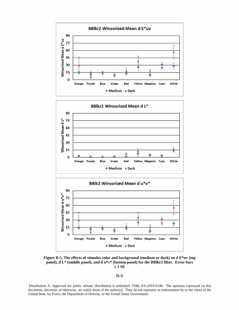
B-6
Distribution A. Approved for public release; distribution is unlimited. TSRL-PA-2019-0149. The opinions expressed on this document, electronic of otherwise, are solely those of the author(s). They do not represent an endorsement by or the views of the United State Air Force, the Department of Defense, or the United States Government.
Figure B-5. The effects of stimulus color and background (medium or dark) on d E*uv (top panel), d L* (middle panel), and d u*v* (bottom panel) for the BBlkr2 filter. Error bars
± 1 SE

B-7
Distribution A. Approved for public release; distribution is unlimited. TSRL-PA-2019-0149. The opinions expressed on this document, electronic of otherwise, are solely those of the author(s). They do not represent an endorsement by or the views of the United State Air Force, the Department of Defense, or the United States Government.
Figure B-6. The effects of each filter and adaptation. The diamonds are the nine unfiltered stimuli. The tail of the arrows are the filtered stimuli and the tip of the arrows are filtered
and adapted predictions
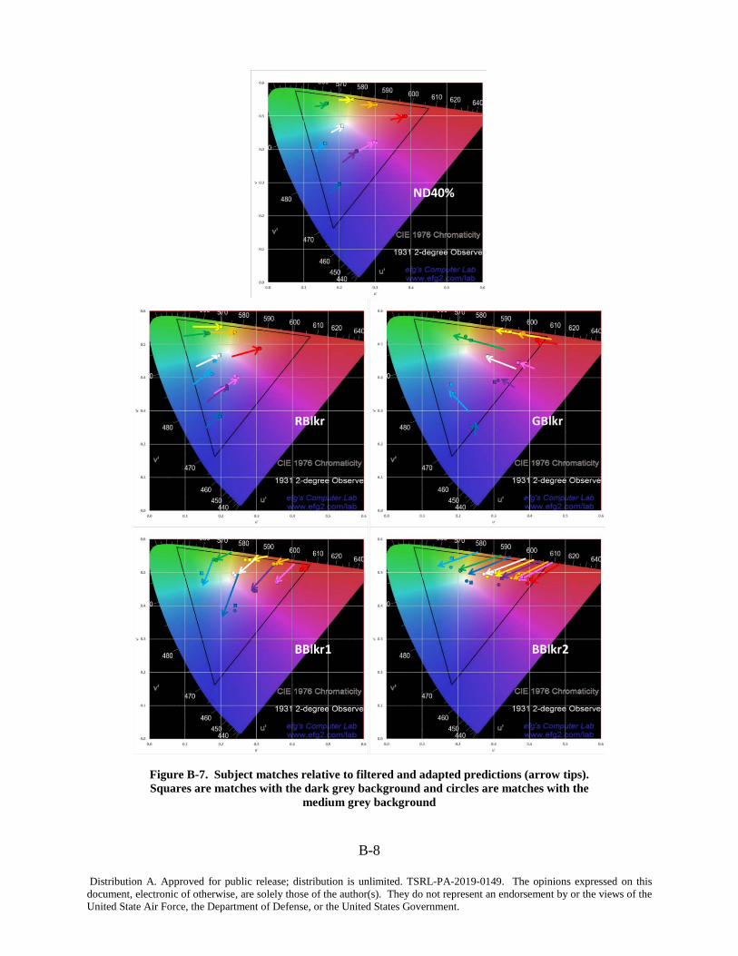
B-8
Distribution A. Approved for public release; distribution is unlimited. TSRL-PA-2019-0149. The opinions expressed on this document, electronic of otherwise, are solely those of the author(s). They do not represent an endorsement by or the views of the United State Air Force, the Department of Defense, or the United States Government.
Figure B-7. Subject matches relative to filtered and adapted predictions (arrow tips). Squares are matches with the dark grey background and circles are matches with the
medium grey background