aggregate recruiting intensity - princeton university
TRANSCRIPT

yl
Aggregate Recruiting Intensity
Alessandro Gavazza
London School of Economics
Simon Mongey
New York University
Gianluca Violante
New York University
Macroeconomics Lunch
Princeton, November 8th 2016

Aggregate recruiting intensityyyl
Ht = AtVαt U1−α
t
Gavazza-Mongey-Violante, "Aggregate Recruiting Intensity" p.1/28hello

Aggregate recruiting intensityyyl
Ht = AtVαt U1−α
t
The component of A accounted for by firms’ effort to fill vacancies
Gavazza-Mongey-Violante, "Aggregate Recruiting Intensity" p.1/28hello

Aggregate recruiting intensityyyl
Ht = AtVαt U1−α
t
The component of A accounted for by firms’ effort to fill vacancies
Macro data
• Large and persistent decline in A in the last recession
• Q1: How much of the decline in A is accounted for by ARI?
Micro data (Davis-Faberman-Haltiwanger, 2013)
• Fast growing firms fill vacancies more quickly
• Q2: What is the transmission mechanism from macro shocks to ARI?
Gavazza-Mongey-Violante, "Aggregate Recruiting Intensity" p.1/28hello

Firm-level hiring technologyyl
Random-matching model hit = qtvit
+ recruiting intensity hit = qteitvit
• JOLTS vacancies - vit
• BLS: “Specific position that exists... for start within 30-days... with active
recruiting from outside the establishment”
Gavazza-Mongey-Violante, "Aggregate Recruiting Intensity" p.2/28hello

Firm-level hiring technologyyl
Random-matching model hit = qtvit
+ recruiting intensity hit = qteitvit
• JOLTS vacancies - vit
• BLS: “Specific position that exists... for start within 30-days... with active
recruiting from outside the establishment”
• Recruitment intensity - eit
1. Shifts the filling rate (or yield) of an open position
2. Costly on a per vacancy basis
• An outcome of expenditures on recruiting activities
Gavazza-Mongey-Violante, "Aggregate Recruiting Intensity" p.2/28hello

Recruiting cost by activityy
Tools 1%
Employment branding services
2%
Professional networking sites
3% Print / newspapers /
billboards 4%
University recruiting 5%
Applicant tracking system
5% Travel 8%
Contractors 8%
Employee referrals 9%
Other 12%
Job boards 14%
Agencies / third-party recruiters
29%
Bersin and Associates, Talent Acquisition Factbook (2011)
- Average cost per hire (at 100+ employee firms): $3,500
Gavazza-Mongey-Violante, "Aggregate Recruiting Intensity" p.3/28hello

From firm-level to aggregate recruiting intensityyl
• Aggregation
Ht = qt
∫
eitvit dλht = qtV
∗t
• Aggregate matching function
Ht = V∗t
αU1−αt = ΦtVt
αU1−αt
• Aggregate recruiting intensity
Φt =
[V∗
t
Vt
]α
=
[∫
eit
(vit
Vt
)
dλht
]α
Gavazza-Mongey-Violante, "Aggregate Recruiting Intensity" p.4/28hello

Transmission mechanism: two channelsyyl
Gavazza-Mongey-Violante, "Aggregate Recruiting Intensity" p.5/28hello

Transmission mechanism: two channelsyyl
1. Composition: macro shock → shift in hiring rate distribution
y
h
n= q̄
ye
y
v
n
• Slow-growing firms recruit less intensively
• Great Recession - large decline in firm entry
Gavazza-Mongey-Violante, "Aggregate Recruiting Intensity" p.5/28hello

Transmission mechanism: two channelsyyl
1. Composition: macro shock → shift in hiring rate distribution
y
h
n= q̄
ye
y
v
n
• Slow-growing firms recruit less intensively
• Great Recession - large decline in firm entry
2. Slackness: macro shock → slacker labor market
h̄
n=
xq
ye
y
v
n
• Firms substitute away from costly hiring measures
• Great Recession - large decline in market tightness
Gavazza-Mongey-Violante, "Aggregate Recruiting Intensity" p.5/28hello

Model yyl
Gavazza-Mongey-Violante, "Aggregate Recruiting Intensity" p.6/28hello

Model yyl
Firm dynamics
• Operate DRS technology
• Idiosyncratic productivity shocks
• Endogenous entry and exit
Gavazza-Mongey-Violante, "Aggregate Recruiting Intensity" p.6/28hello

Model yyl
Firm dynamics
• Operate DRS technology
• Idiosyncratic productivity shocks
• Endogenous entry and exit
Financial frictions
• Borrowing secured by collateral
• Limits to equity issuance
Gavazza-Mongey-Violante, "Aggregate Recruiting Intensity" p.6/28hello
Model yyl
Firm dynamics
• Operate DRS technology
• Idiosyncratic productivity shocks
• Endogenous entry and exit
Financial frictions
• Borrowing secured by collateral
• Limits to equity issuance
Labor market frictions
• Random matching with homogeneous workers
• Recruiting effort e and vacancies v are costly
Gavazza-Mongey-Violante, "Aggregate Recruiting Intensity" p.6/28hello

Valueyfunctionsyl
Let V(n, a, z) be the present discounted value of dividends of a firm withemployment n, net-worth a, and productivity z
Gavazza-Mongey-Violante, "Aggregate Recruiting Intensity" p.7/28hello

Valueyfunctionsyl
Let V(n, a, z) be the present discounted value of dividends of a firm withemployment n, net-worth a, and productivity z
• Exit exogenously or endogenously
V(n, a, z) = ζa + (1 − ζ)max{
a , Vi(n, a, z)
}
• Fire or hire
Vi(n, a, z) = max
{
Vf (n, a, z) , V
h(n, a, z)}
Gavazza-Mongey-Violante, "Aggregate Recruiting Intensity" p.7/28hello

Value functions - Firingyl
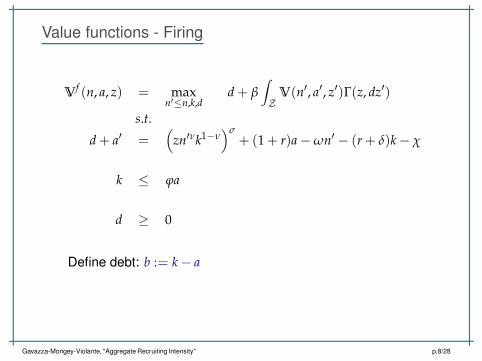
Vf (n, a, z) = max
n′≤n,k,dd + β
∫
ZV(n′, a′, z′)Γ(z, dz′)
s.t.
d + a′ =(
zn′νk1−ν)σ
+ (1 + r)a − ωn′ − (r + δ)k − χ
k ≤ ϕa
d ≥ 0
Gavazza-Mongey-Violante, "Aggregate Recruiting Intensity" p.8/28hello
Value functions - Firingyl
Vf (n, a, z) = max
n′≤n,k,dd + β
∫
ZV(n′, a′, z′)Γ(z, dz′)
s.t.
d + a′ =(
zn′νk1−ν)σ
+ (1 + r)a − ωn′ − (r + δ)k − χ
k ≤ ϕa
d ≥ 0
Define debt: b := k − a
Gavazza-Mongey-Violante, "Aggregate Recruiting Intensity" p.8/28hello

Value functions - Hiringyl
Vh(n, a, z) = max
v>0,e>0,k,dd + β
∫
ZV(n′, a′, z′)Γ(z, dz′)
s.t.
d + a′ =(
zn′νk1−ν)σ
+ (1 + r)a − ωn′ − (r + δ)k − χ − C(e, v, n)
n′ − n = q(θ∗)ev
k ≤ ϕa
d ≥ 0
Gavazza-Mongey-Violante, "Aggregate Recruiting Intensity" p.9/28hello

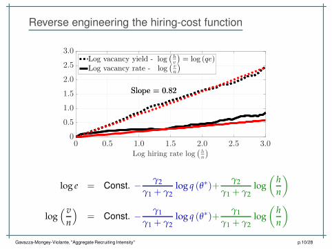
Reverse engineering the hiring-cost functionyl
0 0.5 1.0 1.5 2.0 2.5 3.0Log hiring rate log
(
hn
)
0
0.5
1.0
1.5
2.0
2.5
3.0Log vacancy yield - log
(
hv
)
= log (qe)Log vacancy rate - log
(
vn
)
Slope = 0.82
Gavazza-Mongey-Violante, "Aggregate Recruiting Intensity" p.10/28hello

Reverse engineering the hiring-cost functionyl
0 0.5 1.0 1.5 2.0 2.5 3.0Log hiring rate log
(
hn
)
0
0.5
1.0
1.5
2.0
2.5
3.0Log vacancy yield - log
(
hv
)
= log (qe)Log vacancy rate - log
(
vn
)
Slope = 0.82
C(e, v, n) =
[κ1
γ1eγ1 +
κ2
γ2 + 1
(v
n
)γ2]
︸ ︷︷ ︸
Cost per vacancy
v, γ1 ≥ 1, γ2 ≥ 0
Gavazza-Mongey-Violante, "Aggregate Recruiting Intensity" p.10/28hello

Reverse engineering the hiring-cost functionyl
0 0.5 1.0 1.5 2.0 2.5 3.0Log hiring rate log
(
hn
)
0
0.5
1.0
1.5
2.0
2.5
3.0Log vacancy yield - log
(
hv
)
= log (qe)Log vacancy rate - log
(
vn
)
Slope = 0.82
log e = Const. −γ2
γ1 + γ2log q (θ∗)+
γ2
γ1 + γ2log
(h
n
)
log( v
n
)
= Const. −γ1
γ1 + γ2log q (θ∗)+
γ1
γ1 + γ2log
(h
n
)
Gavazza-Mongey-Violante, "Aggregate Recruiting Intensity" p.10/28hello
Reverse engineering the hiring-cost functionyl
0 0.5 1.0 1.5 2.0 2.5 3.0Log hiring rate log
(
hn
)
0
0.5
1.0
1.5
2.0
2.5
3.0Log vacancy yield - log
(
hv
)
= log (qe)Log vacancy rate - log
(
vn
)
Slope = 0.82Slope = 0.82
log e = Const. −γ2
γ1 + γ2log q (θ∗)+
γ2
γ1 + γ2log
(h
n
)
log( v
n
)
= Const. −γ1
γ1 + γ2log q (θ∗)+
γ1
γ1 + γ2log
(h
n
)
Gavazza-Mongey-Violante, "Aggregate Recruiting Intensity" p.10/28hello

Value functions - Entryyl
• Initial wealth: Household allocates a0 to λ0 potential entrants
• Productivity: Potential entrants draw z ∼ Γ0(z)
• Entry: Choice to become incumbent and pay χ0 start-up costs
Ve(a0, z) = max
{
a0 , Vi (n0, a0 − χ0, z)
}
Selection at entry based only on productivity z
Life cycle: slow growth b/c of fin. constraints and convex hiring costs
Equilibrium
Gavazza-Mongey-Violante, "Aggregate Recruiting Intensity" p.11/28hello

Parameter values set externallyyl
Parameter Value Target
Discount factor (monthly) β 0.9967 Ann. risk-free rate = 4%Mass of potential entrants λ0 0.02 Meas. of incumbents = 1Size of labor force L̄ 24.6 Average firm size = 23Elasticity of matching function wrt Vt α 0.5 JOLTS
Add to the model
• Heterogeneity in DRS σ ∈ {σL, σM, σH}
Calibration strategy
1. Worker flows and labor share
2. Distribution of firm size and firm growth rates
3. Micro-evidence on job-filling and vacancy-posting
4. Entry and exit
5. Leverage for young firms and aggregate economy
Gavazza-Mongey-Violante, "Aggregate Recruiting Intensity" p.12/28hello

Parameter values estimated internallyyl
Parameter Value Target Model Data
Flow of home production ω 1.000 Monthly separ. rate 0.033 0.030Scaling of match. funct. Φ̄ 0.208 Monthly job finding rate 0.411 0.400Prod. weight on labor ν 0.804 Labor share 0.627 0.640
Midpoint DRS in prod. σM 0.800 Employment share n: 0-49 0.294 0.306High-Low spread in DRS ∆σ 0.094 Employment share n: 500+ 0.430 0.470Mass - Low DRS µL 0.826 Firm share n: 0-49 0.955 0.956Mass - High DRS µH 0.032 Firm share n: 500+ 0.004 0.004
Std. dev of z shocks ϑz 0.052 Std. dev ann emp growth 0.440 0.420Persistence of z shocks ρz 0.992 Mean Q4 emp / Mean Q1 emp 75.161 76.000
Mean z0 ∼ Exp(z̄−10 ) z̄0 0.390 ∆ log z: Young vs. Mature -0.246 -0.353
Cost elasticity wrt e γ1 1.114 Elasticity of vac yield wrt g 0.814 0.820Cost elasticity wrt v γ2 4.599 Ratio vac yield: <50/>50 1.136 1.440Cost shifter wrt e κ1 0.101 Hiring cost (100+) / wage 0.935 0.927Cost shifter wrt v κ2 5.000 Vacancy share n < 50 0.350 0.370
Exogenous exit probability ζ 0.006 Survive ≥ 5 years 0.497 0.500Entry cost χ0 9.354 Annual entry rate 0.099 0.110Operating cost χ 0.035 Fraction of JD by exit 0.210 0.340
Initial wealth a0 10.000 Start-up Debt to Output 1.361 1.280Collateral constraint ϕ 10.210 Aggregate debt-to-Net worth 0.280 0.350
Gavazza-Mongey-Violante, "Aggregate Recruiting Intensity" p.13/28hello

Non-targeted momentsyl
Moment Model Data Source
Aggregate dividend / profits 0.411 0.400 NIPA
1Employment share: growth ∈ [−2.00,−0.20) 0.070 0.076 Davis et al. (2010)Employment share: growth ∈ (−0.20,−0.20] 0.828 0.848 Davis et al. (2010)Employment share: growth ∈ (0.20, 2.00] 0.102 0.076 Davis et al. (2010)
Employment share: Age ≤ 1 0.013 0.020 BDSEmployment share: Age ∈ (1, 10) 0.309 0.230 BDSEmployment share: Age ≥ 10 0.678 0.750 BDS
(1.) Firm growth rates are annual and are interior to [−2, 2] so do not include entering andexiting firms
Fig. Average �rm life y le (i) size, (ii) job reation, (iii) fra tion onstrained, (iv) leverage
Gavazza-Mongey-Violante, "Aggregate Recruiting Intensity" p.14/28hello

Hire and vacancy shares by size classyl
1-9 10-49 50-249 250-999 1000+0
0.05
0.1
0.15
0.2
0.25
0.3
0.35
A. Hires
1-9 10-49 50-249 250-999 1000+0
0.05
0.1
0.15
0.2
0.25
0.3
0.35
B. Vacancies
Model, Data - JOLTS 2002-2007
Gavazza-Mongey-Violante, "Aggregate Recruiting Intensity" p.15/28hello

Vacancy and recruitment intensity by ageyl
0 2 4 6 8 10
Age (years)
0
0.2
0.4
0.6
0.8
1
Logdifferen
cefrom
10yearold
A. Cohort average growth and recruitment
Growth rateRecruiting intensityVacancy rate
0 5 10 15
Age (years)
0
0.01
0.02
0.03
0.04
Fractionoffirm
sbyage(m
onthly)
B. Age distributions
Hiring firmsRecruiting intensityVacant positions
Gavazza-Mongey-Violante, "Aggregate Recruiting Intensity" p.16/28hello

Vacancy and recruitment intensity by ageyl
0 2 4 6 8 10
Age (years)
0
0.2
0.4
0.6
0.8
1
Logdifferen
cefrom
10yearold
A. Cohort average growth and recruitment
Growth rateRecruiting intensityVacancy rate
0 5 10 15
Age (years)
0
0.01
0.02
0.03
0.04
Fractionoffirm
sbyage(m
onthly)
B. Age distributions
Hiring firmsRecruiting intensityVacant positions
Young firms exert more recruiting effort: true in Austrian micro-data
Gavazza-Mongey-Violante, "Aggregate Recruiting Intensity" p.16/28hello

Transition dynamics experimentsyl
Trace transitional dynamics of the economy in response to:
• Tightening of financial constraint ↓ ϕ
• Size of shock: match max drop in output (Fernald, 2015)
- Requires 75% drop in ϕ
• Persistence of shock: match half-life of output decline of 3 years
- Monthly persistence of ϕ shock of 0.97
Gavazza-Mongey-Violante, "Aggregate Recruiting Intensity" p.17/28hello

Transition dynamics experimentsyl
Trace transitional dynamics of the economy in response to:
• Tightening of financial constraint ↓ ϕ
• Size of shock: match max drop in output (Fernald, 2015)
- Requires 75% drop in ϕ
• Persistence of shock: match half-life of output decline of 3 years
- Monthly persistence of ϕ shock of 0.97
In the paper: examine also productivity shock
Ma ro TD
Gavazza-Mongey-Violante, "Aggregate Recruiting Intensity" p.17/28hello

Transition dynamics yl
0 1 2 3 4 5 6Years
-1
-0.5
0
0.5
1
Logdeviationfrom
date
0
A. US Data 2008:01 - 2014:01
0 1 2 3 4 5 6Years
-1
-0.5
0
0.5
1
Logdeviationfrom
date
0
B. Model - Finance ϕ-shock
Vacancies Vacancy yield Unemployment Job finding rate Agg. recruiting intensity
Fig. Ma ro variables (i) output, (ii) debt/output, (iii) labor produ tivity
Gavazza-Mongey-Violante, "Aggregate Recruiting Intensity" p.18/28hello
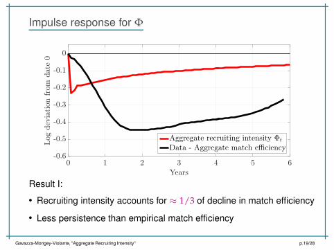
Impulse response for Φyl
0 1 2 3 4 5 6Years
-0.6
-0.5
-0.4
-0.3
-0.2
-0.1
0Logdeviationfrom
date
0
Aggregate recruiting intensity Φt
Data - Aggregate match efficiency
Result I:
• Recruiting intensity accounts for ≈ 1/3 of decline in match efficiency
• Less persistence than empirical match efficiency
Gavazza-Mongey-Violante, "Aggregate Recruiting Intensity" p.19/28hello

Decomposing Φtyl
Recruiting effort policy
e = Const. × q (θ∗)−
γ2γ1+γ2 ×
(h
n
) γ2γ1+γ2
Aggregate recruiting intensity
Φ =
[∫
e( v
V
)
dλh
]α
Decomposition
∆ log Φ = −αγ2
γ1 + γ2∆ log q(θ∗)
︸ ︷︷ ︸
Slackness effect
+ α∆ log
[∫ (
h
n
) γ2γ1+γ2
( v
V
)
dλh
]
︸ ︷︷ ︸
Composition effect
Gavazza-Mongey-Violante, "Aggregate Recruiting Intensity" p.20/28hello

Decomposing Φtyl
0 1 2 3 4 5 6Years
-0.25
-0.2
-0.15
-0.1
-0.05
0
0.05Logdeviationfrom
date
0
Aggregate recruiting intensity Φt
Slackness effectComposition effect
Result II:
• Slackness effect is dominant
Gavazza-Mongey-Violante, "Aggregate Recruiting Intensity" p.21/28hello

Decomposing Φtyl
0 1 2 3 4 5 6Years
-0.25
-0.2
-0.15
-0.1
-0.05
0
0.05Logdeviationfrom
date
0
Aggregate recruiting intensity Φt
Slackness effectComposition effect
Result III:
• Composition effect is roughly zero
• Why? Constrained vs. unconstrained firms
Gavazza-Mongey-Violante, "Aggregate Recruiting Intensity" p.21/28hello

Understanding vacancy yields by sizeyl
Gavazza-Mongey-Violante, "Aggregate Recruiting Intensity" p.22/28hello

Understanding vacancy yields by sizeyl
0 6 12 18 24
Month
-0.2
0
0.2
0.4
0.6
Logdev.from
date
0
C. Vacancy yield - Data 2008:01-2010:12
Size 1-9Size 1000+
0 6 12 18 24
Month
-0.2
0
0.2
0.4
0.6
Logdev.from
date
0
D. Vacancy yield - Model
Size 1-9Size 1000+
0 6 12 18 24-1.5
-1
-0.5
0
0.5
1
Log
dev.from
date0
A. Recruiting intensity per vacancy
UnconstrainedConstrained
0 6 12 18 240
0.1
0.2
0.3
0.4
0.5
Level
B. Fraction constrained
Size 1-9Size 1000+
Result IV
• Slackness and composition explains vacancy yields by size
Gavazza-Mongey-Violante, "Aggregate Recruiting Intensity" p.22/28hello

Summaryyl
Results
I. Recruiting intensity explains 1/3 of decline in match efficiency
II. Dominant: Slack labor markets reduce need for costly recruiting
III. Strong GE forces limit the role of the composition effect
IV. Slackness and composition explains vacancy yields by size
Gavazza-Mongey-Violante, "Aggregate Recruiting Intensity" p.23/28hello

Summaryyl
Results
I. Recruiting intensity explains 1/3 of decline in match efficiency
II. Dominant: Slack labor markets reduce need for costly recruiting
III. Strong GE forces limit the role of the composition effect
IV. Slackness and composition explains vacancy yields by size
Extensions
1. Effect of changes in sectoral composition of firms over recession
2. Construct an easy-to-measure index of aggregate recruiting intensity
3. Relationship to Kaas & Kircher (2015)
Gavazza-Mongey-Violante, "Aggregate Recruiting Intensity" p.23/28hello
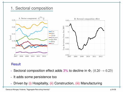
1. Sectoral compositionyl
2007 2008 2009 2010 2011 20120
0.05
0.10
0.15
0.20
0.25
Level
A. Sector component: φ̂γ1
γ1+γ2s
vstVt
ConManTradeProf servEd/HthHospGov
2007 2008 2009 2010 2011 2012-0.04
-0.03
-0.02
-0.01
0
0.01
0.02
Logdeviationfrom
Jan2001
B. Sectoral composition effect
Result
- Sectoral composition effect adds 3% to decline in Φt (0.20 → 0.23)
- It adds some persistence too
- Driven by (i) Hospitality, (ii) Construction, (iii) Manufacturing
Gavazza-Mongey-Violante, "Aggregate Recruiting Intensity" p.24/28hello

2. Approximate index of aggregate recruiting intensityyl
DFH provide an easy-to-compute index of aggregate recruiting intensity
log Φt = log(Ht/Vt)− log qt
d log Φt
d log(Ht/Nt)=
d log(Ht/Vt)
d log(Ht/Nt)−
d log qt
d log(Ht/Nt)
(a) Use firm-level elasticity for first term, ξ = 0.82
(b) Assume second term is small
d log Φt
d log(Ht/Nt)≈ ξ
d log ΦDFHt = ξ × d log(Ht/Nt)
Gavazza-Mongey-Violante, "Aggregate Recruiting Intensity" p.25/28hello
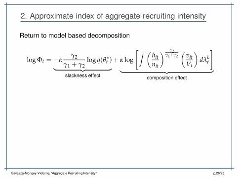
2. Approximate index of aggregate recruiting intensityyl
Return to model based decomposition
log Φt = −αγ2
γ1 + γ2log q(θ∗t )
︸ ︷︷ ︸
slackness effect
+ α log
[∫ (
hit
nit
) γ2γ1+γ2
(vit
Vt
)
dλht
]
︸ ︷︷ ︸
composition effect
Gavazza-Mongey-Violante, "Aggregate Recruiting Intensity" p.26/28hello

2. Approximate index of aggregate recruiting intensityyl
Return to model based decomposition
log Φt = −αγ2
γ1 + γ2log q(θ∗t )
︸ ︷︷ ︸
slackness effect
+ α log
[∫ (
hit
nit
) γ2γ1+γ2
(vit
Vt
)
dλht
]
︸ ︷︷ ︸
composition effect
GMV
(a) Model tells us the composition effect is approximately zero
d log ΦGMVt = α
γ2
γ1 + γ2× (1 − α)× d log θ∗t
(b) Elasticity of θ∗t to θt from transition dynamics
d log ΦGMVt = α
γ2
γ1 + γ2× (1 − α) εθ∗,θ
︸︷︷︸
≈1.5
×d log θt
Gavazza-Mongey-Violante, "Aggregate Recruiting Intensity" p.26/28hello

2. Approximate index of aggregate recruiting intensityyl
2001 2002 2003 2004 2005 2006 2007 2008 2009 2010 2011 2012 2013 2014 2015 2016-0.6
-0.5
-0.4
-0.3
-0.2
-0.1
0
0.1
0.2
LogAggregate
RecruitingIntensity
Aggregate match efficiencyDFH measure of recruiting intensityGMV measure of recruiting intensityGMV + Sectoral component
Gavazza-Mongey-Violante, "Aggregate Recruiting Intensity" p.27/28hello

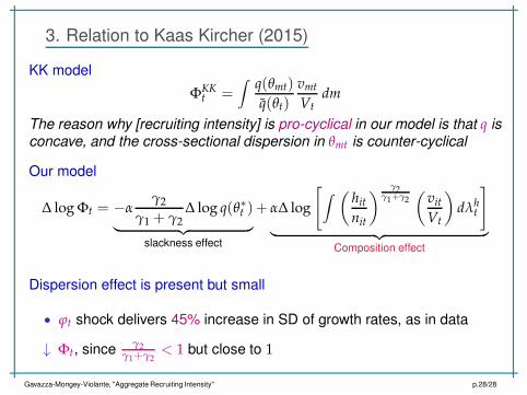
3. Relation to Kaas Kircher (2015)yl
KK model
ΦKKt =
∫q(θmt)
q̄(θt)
vmt
Vtdm
The reason why [recruiting intensity] is pro-cyclical in our model is that q isconcave, and the cross-sectional dispersion in θmt is counter-cyclical
Gavazza-Mongey-Violante, "Aggregate Recruiting Intensity" p.28/28hello
3. Relation to Kaas Kircher (2015)yl
KK model
ΦKKt =
∫q(θmt)
q̄(θt)
vmt
Vtdm
The reason why [recruiting intensity] is pro-cyclical in our model is that q isconcave, and the cross-sectional dispersion in θmt is counter-cyclical
Our model
∆ log Φt = −αγ2
γ1 + γ2∆ log q(θ∗t )
︸ ︷︷ ︸
slackness effect
+ α∆ log
[∫ (
hit
nit
) γ2γ1+γ2
(vit
Vt
)
dλht
]
︸ ︷︷ ︸
Composition effect
Dispersion effect is present but small
• ϕt shock delivers 45% increase in SD of growth rates, as in data
↓ Φt, since γ2γ1+γ2
< 1 but close to 1
Gavazza-Mongey-Violante, "Aggregate Recruiting Intensity" p.28/28hello
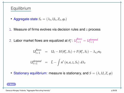
Equilibriumyl
• Aggregate state St = (λt, Ut, Zt, ϕt)
1. Measure of firms evolves via decision rules and z process
2. Labor market flows are equalized at θ∗t : Uflowst+1 = Udemand
t+1
Uflowst+1 = Ut − H(θ∗t , St) + F(θ∗t , St)− λe,tn0
Udemandt+1 = L̄ −
∫
n′ (n, a, z, St) dλt
• Stationary equilibrium: measure is stationary, and S = (λ, U, Z, ϕ)
Ba k
Gavazza-Mongey-Violante, "Aggregate Recruiting Intensity" p.28/28hello

Average life cycle of firms in the modelyl
0 1 2 3 4 5
Age (years)
0
0.05
0.10
0.15
0.20
0.25B. Job creation and destruction
Job creation rateJob destruction rate
0 5 10 15
Age (years)
0
100
200
300
400A. Average size
High σH
Med σM
Low σL
0 1 2 3 4 5
Age (years)
0
0.2
0.4
0.6
0.8
1C. Fraction of firms constrained
0 5 10 15 20
Age (years)
0
5
10
15D. Average leverage
Ba k
Gavazza-Mongey-Violante, "Aggregate Recruiting Intensity" p.28/28hello

Transition dynamics - Macroyl
0 1 2 3 4 5 6Years
-0.25
-0.2
-0.15
-0.1
-0.05
0
Logdeviationfrom
date
0
A. Productivity Z-shock
0 1 2 3 4 5 6Years
-0.25
-0.2
-0.15
-0.1
-0.05
0
Logdeviationfrom
date
0
B. Finance ϕ-shock
Debt/Output (B+t /Yt) Labor Productivity (Yt/Nt) Entry
Ba k
Gavazza-Mongey-Violante, "Aggregate Recruiting Intensity" p.28/28hello