aggregative mechanics of rigid body systemsmechanics-konoplev.com/aggregative_mechanics_of... ·...
TRANSCRIPT

Aggregative mechanics of rigid body systems V.A. Konoplev
Sankt-Petersburg 1996

Contents
Preface ix
1 Kinematics of multibody systems 11.1 Linear space of equipollent systems of line vectors . . . . . . . 1
1.1.1 Equation of the kinematics on the group Lt(R,6) . . . 101.2 Graph of a tree-like multibody system . . . . . . . . . . . . . . 13
1.2.1 Examples of multibody systems . . . . . . . . . . . . . . 171.3 Kinematic equations of (µ, k − 1; lk)-th kinematic pair . . . . . 22
1.3.1 Examples of equations of kinematic pairs . . . . . . . . 251.4 Kinematics of Hooke-elastic pair . . . . . . . . . . . . . . . . . 271.5 Kinematic equations of lk-th element . . . . . . . . . . . . . . . 29
1.5.1 Examples of kinematic equations of kinematic pairs . . 301.6 Kinematic equations of a tree-like multibody system . . . . . . 33
1.6.1 Examples of constructing configuration matrices . . . . 351.6.2 Examples of kinematic equations of kinematic pairs . . 371.6.3 Examples for constructing parastrophic matrices . . . . 38
2 Equations of motion for a multibody system 412.1 Equations of motion of an element of a multibody system . . . 41
2.1.1 Equations of motion of an element of a system carry-ing dynamically non-balanced and asymmetric rotatingbodies . . . . . . . . . . . . . . . . . . . . . . . . . . . . 45
2.1.2 Equations of motion of an element of a multibody sys-tem in inertial medium . . . . . . . . . . . . . . . . . . 46
2.2 Equations of motion of a tree-like multibody system . . . . . . 472.2.1 Equations of motion of double pendulum . . . . . . . . 50
2.3 Equations of Hooke-elastic body system motion . . . . . . . . . 532.4 Effective forms of equations of multibody system motion . . . . 552.5 Determination of preplanned control with the help of forward
and backward sweep methods . . . . . . . . . . . . . . . . . . . 66
v

vi Chapter 1
2.6 Algorithm for constructing equations of motion based on for-ward and backward sweep methods . . . . . . . . . . . . . . . . 69
3 Analytic transvective forms of dynamic equations in the Cauchyform 753.1 Matrix realization of Gauss method . . . . . . . . . . . . . . . . 763.2 Analytic transvective forms of inertia matrix and its inverse . . 763.3 Analytical transvective Cauchy form of motion equations for a
tree-like system . . . . . . . . . . . . . . . . . . . . . . . . . . . 793.4 Computer complexity of the algorithms . . . . . . . . . . . . . 80
4 Differential equations of constraints of multibody systemswith the external medium bodies 854.1 State of the art . . . . . . . . . . . . . . . . . . . . . . . . . . . 854.2 Kinematics of pairs ‘the system bodies –the external medium
ones’ . . . . . . . . . . . . . . . . . . . . . . . . . . . . . . . . . 864.3 Differential equations of time-invariant constraints . . . . . . . 914.4 Differential equations of time-varying constraints . . . . . . . . 954.5 Differential equations of constraints of multibody systems with
loops . . . . . . . . . . . . . . . . . . . . . . . . . . . . . . . . . 99
References 101
Notation 105

Preface
The main theme of this book is Computer-Aided Modeling concerned withthe Mechanics of Multibody Systems branch of General Mechanics. It bringstogether efforts of specialists in the field of mechanics and information scienceto solve the basic problem (see, e.g., Gerdt et al. 1980, Grosheva et al. 1983,Klimov et al. 1989):
to develop theoretical foundations and applied issues of a new field ofthe human knowledge based on bringing together (‘mutual diffusion’) me-chanics, in particular, the multibody system mechanics, and the branch ofinformation science which is commonly named Computer Algebra.
The above-mentioned problem has been studied in two directions (see Wit-tenburg 1977, Medvedev et al. 1978, Gerdt et al. 1980, Grosheva et al. 1983,Konoplev 1986a, Arais et al. 1987, Velichenko 1988, Klimov et al. 1989):
− the implementation of computer algebra methods in the classical mechan-ics with the aim of developing theoretical and software tools which areintended to replace the traditionally human work in deriving mechanicalsystems motion equations in Newton-Euler, Lagrange, Appel and Hamil-ton forms;
− the development of new mathematical formalisms in mechanics to pro-duce computer-aided algorithms suitable for the use of computer algebramethods and symbolic computation software.
In recent time the trend has been toward bridging the gap between thesetwo approaches. The book contains the results of the development of a newcomputer-aided mathematical formalism of the multibody system mechanicswhich may be easily implemented with the use of computer algebra tools forsymbolic computations and of standard software for numerical ones.
The efficiency of the represented formalism is determined by the followingfacts:
− The algorithms are universal in the sense that analytical and numericalforms of multibody system mechanical models are constructed indepen-
ix

x Preface
dently of one another, i.e., these algorithms may be used for constructinganalytical and, independently, numerical forms of models bypassing thestage of constructing scalar equations.
− The algorithms provide the efficient solution of direct problems in themechanics of multibody systems (with the help of the sweep method).
− There are many efficient recurrent procedures.
− There is no need to derive previously analytical forms of any particularfunctionals (such as Lagrangian, Hamiltonian), the Gauss function, theAppel function and so on.
− There is no need to exploit symbolic differentiating tools, since the al-gorithms contain no such differential operators as Christoffel symbols,three-indexed symbols of Boltzmann, the Jacoby matrix and so on. Alloperations are performed with the use of readily available algebraic tools.
− Where bodies of a system are linked with external bodies, there is no needto derive equations of holonomic and non-holonomic (time-invariant andtime-varying) constraints and computer calculation of the correspondingJacoby matrix for these purposes. To this end, only the matrices whichare derived during the construction of motion equations are used.
− The method of indexing that is oriented to multibody systems with tree-like structure is developed.
− The methodology provides the possibility of taking into account the pres-ence of rotating bodies linked to bodies of a system in the case where thereverse linkage to carrier is absent, as well as the influence of an inertialmedium (e.g., water when the flow is potential) by without significantloss of efficiency of algorithms.
− The derivation of Hooke-elastic multibody system motion equations isprovided.
− Methods of deriving an inertia matrix and its inverse in the form of mul-tiplication of simple matrices (transvective and diagonal) are proposed.
− A method of direct derivation of analytical forms of multibody systemmotion equations in the Cauchy form is developed without computing aninertia matrix and inverting it.
− Practically full parallel processing is provided.
− Work expenditure is minimized.
The book is written on base of the author’s study of the problems knownas classical in mechanics and control theory. It is organized as follows. InChapter 1 we focus on some general issues that are very important in formingmathematical models in the multibody system mechanics. Many method-ologies for description of rigid multibody systems have been proposed in thepast. One of them is based on application of dual vectors and matrices in rigidbody dynamics: in the last thirty years a growing number of investigationsconcerning this topic have appeared in the literature (see, e.g., Angeles et al.1997). Dual vectors (screws) supply us with the description of a multibody
Preface xi
system that does not suffer from singularities as in the case, e.g., of Eulerangles. We present the results of our elaboration of a new mathematical for-malism of the multibody system kinematics which is based on the concept ofa line vector (Brand 1947, Berezkin 1974). We avoid using the common ter-minology of screw theory (Dimentberg 1965, Murray et al. 1993, Selig 1996),as the essence of our approach appears as crucially different and more sim-ple. In particular, equipollent systems of line vectors generate 6-dimensionallinear spaces of binary vectors with respect to various reduction centers. Af-ter introducing bases, we arrive at the coordinate space R6 where a groupof motions such as translations and rotations defines isomorphism betweencoordinate representations of these spaces (Konoplev 1987a). This group actsmultiplicatively, as distinct from the analogous group of translations whichacts additively on R3. The multiplicative group of motions permits us to giveefficient tools for defining binary vectors in various frames (for an arbitrarynumber of intermediate motions). This fact is of importance as the maincontent of the multibody system kinematics and dynamics is in constructingtwists and wrenches (kinematical, kinetic and dynamic binary vectors) as inan inertial frame of reference so in frames attached to system bodies.
After introducing the operation of differentiating on the group of motions, weobtain an algebraic apparatus for calculating velocities and quasi-velocities ofbodies. This permits us to keep the mathematical prerequisites to a minimumand to construct algebraic, physically pictorial models of multibody systemssuitable for computer implementation in symbolic and numerical forms.
A multibody system consists of three levels: kinematical pairs, kinematicalchains of kinematical pairs, and the whole system of kinematic chains (Kono-plev 1986b,c). Preliminary studies have showed that the goal of mathematicalformalization of the multibody system mechanics and, in particular, of thekinematics, together with the efficient apparatus of corresponding computercalculations, may be achieved with the help of system analysis methodology(modular methodology) (Messarovich et al. 1978, Konoplev 1986a).The methodology of system analysis is efficiently used where equations (ormodules in the corresponding terminology), describing the behavior of a sys-tem on each levels, may be derived from the analogous equations, representingits behavior on the previous level. In such cases, the equations, describing thebehavior of the whole system, appear to be comprised of equations (modules)of previous levels. If there exists an algorithm of module construction for thelowest level system, which possesses an efficient computer implementation,then it turns out that the computer implementation of equation constructionfor the whole system is more efficient then any other algorithm.
Kinematical equations of a kinematical pair, a kinematical chain and thewhole system on the first, second and third levels, respectively, are relationsbetween quasi-velocities and generalized velocities (redundant in the generalcase) and play role of the above-mentioned modules. The computer algorithm

xii Preface
of deriving the third level module from the first level modules, i.e., kinematicalequations of the whole system, defines the graph of the system, which isrepresented by a two-line array of zeros and units.
The apparatus of the theory developed in the chapter consists of kinematicalequations (kinematical modules) of all levels. The notion of a twist and thegroup of motions of binary vectors form the basis of this theory. We give thecorresponding algorithms in compact, geometrically and physically pictorialmatrix form readily implemental on a computer for symbolic and numericalcalculation. Of course, these equations are equivalent to known vector equa-tions, but, where the number of intermediate motions is greater than three orfour, the vector equations, being written in scalar form, are too cumbersome(Konoplev 1984, 1987a).
At the end of the chapter, we introduce the parastrophic matrix of a multibodysystem. This matrix transforms generalized velocities into quasi-velocities ofbodies, providing kinematical equations of the system. The parastrophic ma-trix is a basic mathematical element of the theory. It contains the informationon the system kinematical structure, axes, mechanical and functional config-urations of the system. The parastrophic matrix undoes wrenches of internalreactions in any multibody system subjected to holonomic constraints andextracts control and friction forces, acting on mobility axes of the system.
In Chapter 2, we present the development of the dynamics of multibody sys-tems. As in the case of the kinematics, the system analysis is taken as thebase of methodology: at first, equations of motion of single rigid bodies inlinear space of quasi-velocities are derived (the first-level dynamic modules)in the special matrix form, then equations of motion of kinematical chains(the second-level dynamic modules) and finally equations of motion of thewhole system (the third-level dynamic modules) are obtained.We then derive equations of motion of a multibody system relative to gener-alized coordinates as a result of eliminating quasi-velocities from the dynamicmodule of the system with the use of kinematical equations (Konoplev 1989a,1990, Konoplev et al. 1991).
We obtain equations of motion for a single rigid body with dynamically un-balanced and asymmetric rotating flywheels placed on it under conditions inwhich carrier motion has no influence on their rotation. The influence of aninertial external medium on system motion is taken into account (e.g., water,provided that the flow is potential) (Konoplev 1987b and 1989b,c).
Deriving dynamic equation of Hooke-elastic bodies motion and constructing(with its use) equations of ‘fast’ and ‘slow’ motions (taking into account cross-effects) are also considered in the first part of Chapter 2 (Konoplev et al.1991).
The second part of Chapter 2 is devoted to the problem of work expendi-ture for the algorithms of constructing multibody system equations. Thequadratic, in the degree of freedom, algorithm for inertia matrix calculation

Preface xiii
and two linear algorithms for the quadratic, in the generalized velocities terms,calculation are obtained. We propose efficient algorithms, yielding the solu-tion for the so called inverse problem of the multibody system dynamics,which consists in the calculation of reactions between bodies of the systemand control inputs in joints, given values of generalized coordinates and veloc-ities. The labor content for each of the algorithms presented is estimated forthe symbolic and numerical forms. To illustrate algorithms implementation,motion equations for a double pendulum with a sliding hanger are derived inthe symbolic form.
The theoretical results presented in the chapter are illustrated by numerousfully considered examples, such as a gyroscope on an inclined base, a flywheelinstalled on a rigid body, a double pendulum with a sliding hanger, a ma-nipulator, a walking machine, and a test bench (Okhotsimsky et al. 1984,Konoplev 1989, Konoplev et al. 1989, 1992a, Belkov 1992). We have studiedthe above-mentioned mechanisms using computer simulation at the requestof industrial firms.
Thus, because the equations of multibody system motion, introduced in Chap-ter 2, contain only constant inertia matrices and the parastrophic matrix, thedefinition of the latter immediately leads to construction of kinematical equa-tions and motion equations (Konoplev 1989a, 1990, Konoplev et al. 1991).
In Chapter 3, we continue to study the problem of reducing the labor contentfor algorithms of motion equation derivation. It is known (Gantmacher 1964,Suprunenko 1972, Skornyakov 1980 and 1983) that the general linear grouphas the system of generators (transvective and diagonal matrices). Here wegive two algorithms for deriving an inertia matrix and its inverse in the formof multiplications of the above-mentioned simplest matrices. This permitsus to bypass constructing an inertia matrix and to define the symbolic andnumerical forms of its inverse immediately. As a result, we derive the motionequations of a multibody system at once in the Cauchy form (Konoplev 1994,1995).
Estimating the labor content for algorithms for symbolic and numerical formsof matrix representation we see that one of them is the most efficient algorithmwhen the system degree of freedom is greater than 27-30.
In Chapter 4, a new efficient method for constructing differential equations ofholonomic and non-holonomic, time-invariant and time-varying constraints isdeveloped. It is customary to derive the above-mentioned equations in twostages. First, equations of constraints are written and then the Jacoby matrixof holonomic constraints is derived (Nikulin et al. 1983). With the use ofthis matrix and that of linear non-holonomic constraints, differential equa-tions of constraints are constructed. These equations are used for eliminatingLagrange multipliers from redundant equations of motion. If there are manyconstraints and the system degree of freedom is great, the construction ofthese matrices is tedious. We propose a new, in essence, approach to solv-

xiv Preface
ing this problem. The above-mentioned sequence of operations is replacedwith the inverse one. It turns out that the modular technology of construct-ing multibody system motion equations permits us to derive reaction vectorsof external bodies incidentally during construction of motion equations, inparticular, when determining the parastrophic matrix of the system. It onlyremains to write differential equations of constraints with the use of this ma-trix. Thus the problem of cumbersome analytical construction of constraintequations, as well as the Jacoby matrix computation of each step of numericalintegration of motion equations, is completely removed (Konoplev 1989b and1992).
With the help of this methodology, an algorithm for constructing motionequations for a multibody system with internal chain-loops is elaborated.
The book does not review the literature. There are two reasons for this. In thefirst place, it is impossible to do this in full measure, since the list of relevantpublications is enormous and the number of books and papers on multibodysystem mechanics is steadily growing. Secondly, the results connected withmechanical modeling (the aggregative mechanics) given here does not relyon any works known to the authors. Nevertheless, it is necessary to list theauthors (additional to the above-mentioned Wittenburg 1977, Medvedev etal. 1978, Gerdt et al. 1980, Grosheva et al. 1983, Konoplev 1986a, Araiset al. 1987, Velichenko 1988, Klimov et al. 1989), whose works are uncon-ventional: V.V. Akselrod, A.V. Bansh’ikov, L.A. Burlakova, A.B. Byachkov,L. Chang, M.A. Chubarov, Yu.N. Chelnokov, A.I. Filaretov, F. Freudenstein,H.P. Frisch, A.S. Gorobtsov, T.J. Haug, J.M. Hollrbach, R.L. Huston, R.S.Hwang, V.D. Irtegov, T.R. Kane, A.I. Korzun, G.P. Kulvetis, V.A. Kutergin,E.E. Lavendel, C.S.G. Lee, V.V. Malanin, D. Orin, B. Paul, W. Schiehlen,L.I. Shtejnwolf, A.M. Shulgin, M.W. Walker, O. Wallrapp, P.Y. Willems, J.T.Wang, L. Wang, L. Woo, A.T. Zaremba, among others (we apologize to thosewhom we omit to mention).
The main part of the book is based on lectures that the author has been givingon elective special courses in two departments of the Baltic State TechnicalUniversity (St Petersburg).
The present volume may successfully be used as an introduction to the me-chanics of rigid bodies, it is distinct, however, in that the flavor is decidedlyone of applied mathematics. It also covers details of various extensions ofthe theory and recent research results in mechanics. Readers’ familiarity withreal vectors and matrices, with systems of ordinary differential and differenceequations and with basics of real, complex and functional analysis is presup-posed.
The book will appeal to a wide circle of specialists, including professionalmathematicians interested in modern mathematical formalization of mechan-ics, as well as mechanical engineers, graduates and post-graduate students.They will be able to find numerous efficient algorithms for solving actual

Preface xv
problems in the field of multibody systems, detailed explanations and exam-ples.
The authors thank Academicians of the Russian Academy of Sciences D.M.Klimov, D.E. Okhotsimsky and Corresponding Member V.F. Juravlev forrepeated critical discussions on the aggregative mechanics issues, and Prof.Yu.F. Golubev and Prof. A.P. Makreev for the support given at decisivemoments for the future of computer-aided methods described in the book.

xvi
Chapter 1
Kinematics of multibody systems
1.1. Linear space of equipollent systems of line vectors
It is well known that a system of forces acting on a rigid body generates thesum and the total moment considered with respect of a certain point calledthe center of reduction. Treating the sum and the moment as an aggregate oftwo free vectors we may say about a so called binary vector. This notion isvery near to that of a dual vector or screw (Dimentberg 1965, Murray et al.1993, Selig 1996, Angeles 1997) being in the base of analytical theory of screws(screw theory). However the difference existing between these notions leads tothat our theory differs from screw theory in the same degree as real analysisonR2 from complex analysis. In particular, introducing specific notions of theconventional calculus of screws (such as a principal axis, a spiral products, alinear complex, a spiral affinor, analytical functions of dual vectors and so on)is not be necessary, as we need only the main object of the multibody systemkinematics: a multiplicative group of motions (translations and rotations) inthe linear space R6 defining isomorphism between coordinate representationsof binary vector spaces. In a rather natural way, this yields us very convenientcomputer-aided tools for using equipollent systems of line vectors.
Vectorial objects
Physical magnitudes characterized with the help of one real number are calledscalars. We may easy give examples of scalars: time, angle, length, volume,electrical resistance, mass, work, etc. Some of them can be supplied withsign but it is not essential. On the other hand there are many magnitudessuch that their description cannot be introduced by means of one number.Magnitudes such as velocity, acceleration and force are called vectorial. Inthe simplest case a vector is introduced as a line segment in which the initialpoint is distinguished from the terminal one, the former being also called apoint of application. Points are classified as zero vectors.
1
2 Chapter 1
There are various categories of vectors. A vector of the first category – abounded vector – is given above with fixing its initial and terminal points.This way of (affine) definition does not use the notion of length. With thehelp of some metric a bounded vector can be characterized by the followingelements:
− an initial point;− a direction;− a length (norm).
The classical example of bounded vectors can be vectors of some physical field,e.g., the Earth’s gravitational one.
A vector of the second category – a line vector – is defined by the fol-lowing elements:
− a straight line along which this vector is directed;− a sense;− a length (norm).
In other words, a line vector is defined as a class of equivalence: the set ofbounded vectors having the same line of action, sense and length. The usualmechanical example of a line vector is force: it is characterized by its value,the line of action and sense while its point of application is arbitrary on thisline (see the axioms of statics in the Introduction).
At last, a vector of the third category – a free vector – is given by thefollowing elements:
− a direction;− a length (norm).
In other words, any free vector is defined as a class of equivalence: the setof bounded vectors having the same direction, sense and length. The classicmechanical example of a free vector is translation of a rigid body from onestate into another: its points are replaced in the same direction and at thesame distance, i.e., it is characterized by its value and the line of action whileits point of application is not of importance.
In every separate case of using vectorial objects their category must be estab-lished.
Systems of line vectors
From the mathematical point of view such variety of vectorial objects forcesus to work out specific rules in order to handle with them. We assume thatthe fundamentals of geometrical theory of free and line vectors is known (see,e.g., Berezkin 1974). In particular, free vectors submit to the linear spaceaxiomatics (it is assumed to be known). Any three linear independent vectorscan be used as a basis for introducing a coordinate space that permits us tomake a step from geometry ideas to algebraic ones. With fixing of a certain
Kinematics of multibody systems 3
origin we may introduce the corresponding frame and treat bounded vectorsas difference between radius vectors of their initial and terminal points.
However this mathematical apparatus gives nothing for line vectors as, ingeneral, we have no idea what sum of two line vectors is. At the same timeit is easy to see that any force system satisfies to the linear space axioms(recall that, in the multibody system mechanics, any force is a line vector):we may stretch or shrink all vectors of any system with the help of a certainreal multiplier α and form the union (or difference) of any two systems.
Let Λ be the set of all line vectors. Consider two systems hα = λk ⊂ Λ, k ∈K(α) and hβ = λk ⊂ Λ, k ∈ K(β) of line vectors where K(α) and K(β)are some sets of naturales.
Definition 1.1 The systems hα and hβ, K(α) 6= K(β), of line vectors aresaid to be equipollent
hα ∼ hβ
if they determine the same sum x and total moment µ (with respect to thesame point of reduction).
The pair of vectors x and µ can be used for constructing various models of theclass of equipollent systems. E.g., in the conventional calculus of screws, thispair defines a so called dual vector or screw x+ ωµ where ω is such operatorthat ω2 = 0 (Dimentberg 1965, Angeles 1997). Below a simpler computer-aided model is constructed (we do not aim to discuss here screw calculus aswe wish to keep the mathematical prerequisites to a minimum).
Notation 1.1 Henceforth
− D3 is 3-dimensional space of points and V3 is 3-dimensional space offree vectors associated with it;− a given line vector λ ∈ Λ, x ∈ V3 is the free vector having the samelength, direction and sense as λ;− a given a ∈ D3, l
xa is the action line of λ (i.e., the straight line passing
through the point a in parallel to the vector x), xa is the bounded vectorgenerated by reducing x to the point a;− a point Oσ ∈ D3 is chosen as a so called center of reduction;
− (−−−→Oσ, a) is the bounded vector with the terminal point a (here it is possiblethat a = Oσ);− raσ is the free vector with the same length, direction and sense as
(−−−→Oσ, a).
Define the moment (free vector) of xa with respect to Oσ
µxaσ = raσ × x (1.1)

4 Chapter 1
where the symbol × means the vector product of free vectors.
As a line vector is defined as the class of equivalence for bounded vectors beingsituated on the corresponding straight line, we may reduce the free vector xto any point l ∈ lxa. It is well known that its moment (with respect to Oσ) isequal to µxaσ, i.e.,
rlσ × x = µxaσ (1.2)
where rlσ is the free vector with the same length, direction and sense as (−−→Oσ, l).
This fact does not depend on choosing l ∈ lxa. That is why we have reasonsthe free vectors x and µxaσ to be used for describing the line vector λ (beingsituated on the line lxa of action).
Thus we see that line vectors can be also defined as a class of equivalence forbounded vectors having the same line of action, sense, length and the samemoment with respect of any point (Dimentberg 1965).
Definition 1.2 We shall say that a line vector λ is reduced to the center Oσ
if the aggregate (the ordered couple of Plucker vectors)
lxaσ = col x, µxaσ (1.3)
is computed.
We defined lxaσ as an element of the Cartesian product of V3 ×V3 (while itbelongs to V3+V3, too) as later on we shall use other elements of V3 ×V3.
Proposition 1.1 The set of aggregates is not a linear space.
Proof Indeed, consider a free vector y ∈ V3 and take two points a and bsuch that µyaσ 6= µybσ. Then there are two aggregates (generated by the free
vectors y and −y with the parallel action lines lya and l−yb ) such that their
sum is col y − y, µyaσ − µybσ where the first component is equal zero, and
the second component is not equal zero. But according to relation (1.1) it isimpossible (the second component must be equal zero, too). Thus this sumis no aggregate. 2
Consider the set Λ of all lines vectors and construct the corresponding setof aggregates (with respect to the given center Oσ). Due to the fact thatµxaσ = µ
xlσ for any l ∈ lxa, for the sake of brevity we shall often omit the index
a in the notation of aggregates and their line of action.
Definition 1.3 Let hα = λk ⊂ Λ, k ∈ K(α) be a system of line vectorswhere K(α) is some set of naturales. Then the sum
hσα =X
k∈K(α)lxσk (1.4)
(of the aggregates defined with respect to the given center Oσ) is called a binaryvector.

Kinematics of multibody systems 5
In particular, a binary vector is an aggregate if the aggregates composing thisvector have action lines intersecting each other in one point a: lxaσ + l
yaσ =
col x + y, raσ × (x + y) = lx+yaσ as the set of aggregates with action lines,intersecting each other in one point, is a linear space.
Proposition 1.2 The set Hσ of all binary vectors is a 6-dimensional linearspace.
Proof The amount of all sums of aggregates, i.e., binary vectors, is a sumof aggregates, i.e., a binary vector, too. As to the set dimension it is easy tochoose six (orthonormal) vectors being its basic ones. 2
Thus we may treat any aggregate as a special case of the binary vector gen-erated by one line vector.
Proposition 1.3 The set H of equipollent systems of line vectors is isomor-phic to the linear space Hσ.
Let us finish this section with pointing out the simplest system in a givenequipollent system of line vector. This question is of importance in mechan-ics. In order to give the answer we define the following binary vectors andaggregates.
Definition 1.4 Let us take a free vector x ∈ V3 and two arbitrary points aand b ∈ D3 such that µ
xaσ 6= µxbσ. Then the binary vector hσ being sum of two
aggregates lxaσ and l−xbσ (with respect to the same reduction center Oσ ∈ D3)
is called a couple, and the distance h between the lines lxa and lxb is called the
couple arm.
It is easy to see that
hσ = col 03, rab × x
where rab is the free vector with the same length, direction and sense as (−→b, a);
the symbol 03 means 3-dimensional (free or coordinate) null vector.Note that a couple is invariant with respect to the choice of a reduction center,as it is generated by the free vector x ∈ V3 and depends on the arm of couple.
Definition 1.5 An aggregate and a binary vector defined by
lxσ = col x, 03, hσα = col X
k∈K(α)xk, 03, x 6= 0,
Xxk 6= 0
are called degenerate.
Note that

6 Chapter 1
− an aggregate lxσ is degenerate if its line of action goes through the centerOσ ∈ D3, i.e., the degeneration property depends on the reductioncenter;
− it is not necessary for a degenerate binary vector to be always a sum ofdegenerate aggregates.
Let us present the binary vector (1.4) in the form
hσα = col h(1), h(2)σ = col h(1), 03+ col 03, h(2)σ
where first component h(1) ∈ V3 is called the sum of the system (or the sum
of the vectors xk), and the second component h(2)σ ∈ V3 is called the total
moment with respect to the center Oσ.
It is easy to see that the inner product (h(1), h(2)σ ) does not depend on the
point of reduction. With its help we state the following assertion (see, e.g.,Banach 1951, Berezkin 1974).
Proposition 1.4 Depending on whether the inner product (h(1), h(2)σ ) is dif-
ferent from zero or equal to zero, every α-system of line vectors is equipollentto one of the systems:
− the aggregate col h(1), 03 and a couple having the moment h(2)σ ;− two (skew) aggregates such that one of them has the action line passingthrough the center Oσ;− one aggregate;− the zero vector.
In general, one must not suppose that the simplest system is unique. For thesake of simplicity, classes of equipollent systems of line vectors are usuallyidentified with their simplest representatives.
Group of motions
Relation (1.1) can be used in order to define the two-parametric set of linearoperators Mσ
a : V3 → V3 acting by the law
µxaσ =Mσa x (1.5)
i.e., for any vector x ∈ V3, we have the free vector µxaσ being equal to the
moment of x reduced to the point a with respect to the center Oσ (see theindices of µxaσ). Thus the aggregate (1.3) assumes the form
lxaσ =
·IMσa
¸x (1.6)
where I is the identity operator in V3.
Kinematics of multibody systems 7
Choosing different reduction centers, we may define different operators gener-ating the (1.6)-kind aggregates and the corresponding linear spaces of binaryvectors.Let us consider two linear spaces Hσ and Hτ of binary vectors that generatedwith respect to points Oσ and Oτ ∈ D3, respectively. It is easy to see thatthese spaces are isomorphic, i.e., there is the biunique correspondence definedby the linear operator
Tστ =
·I OMσ
τ I
¸(1.7)
acting from Hτ to Hσ (here the operator Mστ is defined as in relation (1.5);
O is the null operator in V3).It is clear that after introducing bases in Hσ and Hτ we may give the coordi-nate representation of operator (1.7) in the space R6 (it is clear that all thesespaces are isomorphic).
Notation 1.2 Henceforth
− eσ = eσ1 , eσ2 , eσ3 is an orthonormal basis in V3;− a reduction center Oσ ∈ D3 is chosen as the origin of the Cartesianframe Eσ = (Oσ, e
σ);− the basis vectors of Eσ generate the coordinate space R3 and the fol-lowing vectorial matrix
keσk = keσ1 | eσ2 | eσ3k (1.8)
i.e., the matrix with entries being vectors (coordinate columns);− xσ = col xσ1 , xσ2 , xσ3 ∈ R3 is the column of coordinates of any x ∈ V3,i.e., x = keσk xσ;− the cap over the coordinate column, e.g., xσ means the passage from xσ
to the following skew-symmetric matrix
xσ =
0 −xσ3 xσ2xσ3 0 −xσ1−xσ2 xσ1 0
(1.9)
Proposition 1.5 (Konoplev 1987a) Let an aggregate lxaσ be defined (with re-spect to the reduction center Oσ ∈ D3 with the help of a certain free vectorx ∈ V3 reduced to some point a ∈ D3). Then there is the following coordinaterepresentation of lxaσ in R6
lxσaσ = Gσa x
σ (1.10)
where
Gσa =
·EMσσa
¸, Mσσ
a = rσaσ (1.11)

8 Chapter 1
rσaσ ∈ R3 is the coordinate column (see the outer superscript) of the radius
vector (−−−→Oσ, a) in the frame Eσ (see the superscript); E is 3× 3-dimensional
identity matrix (see also Berezkin 1974).
Introduce a new Cartesian frame Eτ = (Oτ , eτ ) with some orthonormal basis
eτ . We may always define the rotation matrix cστ such that
keτk = keσk cστ , xσ = cστxτ (1.12)
(xτ ∈ R3 is the column of coordinates of x in the basis eτ ; |det cστ | = 1).
Notation 1.3 Henceforth
− oστ ∈ V3 is a vector of translation of Eτ (see the subscript) to Eσ
(see the superscript), oσστ is its coordinate column in eσ (see the outersuperscript), and oσστ is the skew-symmetric matrix induced by oσστ (seenotation (1.9));− Hσ
σ and Hττ are the coordinate representations of Hσ and Hτ generated
by the bases eσ and eτ , respectively.
Proposition 1.6 (Konoplev 1987a and 1989a,b) The isomorphism Lστ : Hττ →
Hσσ (= L
στH
ττ ) is defined by the following matrix
Lστ = Tσστ Cσ
τ (1.13)
where
Tσστ =
·E Ooσστ E
¸, Cσ
τ = diag cστ , cστ (1.14)
are matrices of translation and rotation (induced by the translation with thevector oστ and the rotation c
στ ), respectively; O is 3×3-dimensional null matrix.
Proof Suppose lxττk = Gττ x
τk is the coordinate representation of an aggregate
from relation (1.4). Then (see also relations (1.10) and (1.11))
Lστ lxττk = L
στG
ττ x
τk = Tσστ Cσ
τ Gττ x
τk = T
σστ Cσ
τ Gττc
σ,Tτ cστx
τk =
Tσστ Gστ x
σk = G
σσ x
σk = l
xσσk
Taking in account that Lστ is a linear operator and going in the both sides ofthis equality to sums of the (1.4)-kind, we easily obtain the desired result. 2
From the foregoing proposition follows at once that the next assertion holds.
Proposition 1.7 The linear operator Tστ : Hτ→Hσ has the coordinate rep-resentation Tσστ in the basis eσ.

Kinematics of multibody systems 9
Proposition 1.8 The set of all motions Lστ : Hττ →Hσ
σ is the multiplicativegroup
L(R,6) = Lστ : Lστ = T σστ Cστ (1.15)
where σ and τ parameters determining which points the system Λ of all linevectors is reduced to.
Proof It is true because LστLτp = T
σστ Cσ
τ Tττp Cτ
p = Tσστ Cσ
τ Tττp Cσ,T
τ Cστ C
τp =
Tσστ T τσp Cσp = Tσσp Cσ
p = Lσp and (Lστ )−1 = (Tσστ Cσ
τ )−1 = Cσ,T
τ (Tσστ )−1 =CτσT
τσσ Cτ,T
σ Cτσ = T
ττσ Cτ
σ = Lτσ ∈ L(R,6). 2
Remark 1.1 We may treat two objects to be equivalent if there is an Euclid-ean motion transforming one of them into another (Sternberg 1964). It meansthat the set of all spaces of binary vectors can be considered as the class ofequivalence defining an ‘abstract’ binary vector for a given system of line vec-tors. In this sense we may say about computation of a binary vector at acertain point or about its transform from one point at another.
In the multibody system mechanics, we may treat any instantaneous complexmotion as a screw motion along a certain line (this line is a so called screwaxis) (see, e.g., Banach 1951). This case is characterized by the property thatthe first component of some binary vector
hτα = col h(1), h(2)τ
is parallel to the second one. If this is not the case we may always to choosea new reduction center Oσ such that
col h(1), ph(1) = Tστ col h(1), h(2)τ (1.16)
where p is some real number which we shall define below.Indeed, from relation (1.16) follows that there is the relation
ph(1) = oστ × h(1) + h(2)τ
Using the inner product between this vector and h(1) we have
p =(h(1), h
(2)τ )
(h(1), h(1))
On the other hand, the vector product between ph(1) and h(2)τ yields
oστ =h(1) × h(2)τ
(h(1), h(1))

10 Chapter 1
Proposition 1.9 (Dimentberg 1965) The set of all reduction points Oσ such
that the vector h(2)σ is parallel to h(1) is the straight line given by
oστ =h(1) × h(2)τ
(h(1), h(1))+ s h(1)
where s is a scalar parameter.
1.1.1. Equation of the kinematics on the group Lt(R,6)
In general, we shall distinguish two kinds of instantaneous motion of frames:translation and rotation. Let a matrix cστ = cστ (t) define the rotation ofthe basis eτ with respect to the immobile basis eσ considered in the basis eσ
(|det cστ | = 1) (see (1.8) and (1.12)). Denote by Rt ⊂ R3 the one-dimensionalsubspace generated by the unit (time-varying) eigenvector corresponding tothe real (time-invariant) eigenvalue of the matrix cστ . It is clear that theorigin Oτ of the rotating frame Eτ is on Rt. Let P be the two-dimensionalsubspace being orthogonal to Rt and passing through the point Oτ . Suppose
aτ = (−−−→Oτ , a) is the radius vector of a ∈ P. Let us also denote by aτσ and aττ
the coordinate columns of aτ in the bases eσ and eτ of the immovable androtating frames, respectively. Then from aτσ = cστ a
ττ follows that (see (1.12))
aτσ. = cσ.τ aττ = cσ.τ c
σ,Tτ aτσ (1.17)
where (recall) we use convention (0.2) for any differentiable function c = c(t).
Differentiating the relation cσ,Tτ cστ = E we have cσ,Tτ cσ.τ = −(cσ.τ )T cστ . Hencecσ,Tτ cσ.τ = −((cσ,T.τ cστ )
T )T = −(cσ,Tτ cσ.τ )T , i.e., the matrix cσ.τ c
σ,Tτ is skew-
symmetric. Therefore there exists a free vector w = wστ = keσk wσσ
τ =keτk wσττ such that
wσστ = cσ.τ c
σ,Tτ , wσττ = cσ,Tτ cσ.τ (1.18)
where wσστ and wσττ are the coordinate columns of wστ in the bases e
σ and eτ ,respectively.
It is easy to see that the vector wστ defines the instantaneous angular velocityof the basis eτ with respect to the basis eσ whereas the left-hand side of re-lation (1.17) is the coordinate representation of the instantaneous translationvelocity of a ∈ P.Note that the right-hand side of relation (1.17) is coordinate representationof the vector product
vστ = wστ × aτ (1.19)
Thus geometrically we may determine the instantaneous angular velocity asa line vector with the line of action which is defined by the free vectors wσ
τ
and vστ .

Kinematics of multibody systems 11
Let us consider the case where a couple of instantaneous angular velocities wand −w defines the rotations of Eσ and Eτ , respectively. The origins of Eσ
and Eτ are on the action lines of w and −w. Let P be the two-dimensionalsubspace orthogonal to w. Suppose there are the points aσ and aτ where theaction lines of w and −w intersect with P. Introduce the radius vector ofa ∈ P: aσ = (−−→aσ, a) and aτ = (−−→aτ , a).With the help of relation (1.19) we may compute the translation velocities ineach rotation
vσ = w × aσ, vτ = −w × aτ
and the full velocity of the point a
vσ + vτ = w × (aσ − aτ )
where the difference aσ − aτ depends only on the position of the axes ofrotation as it is equal to (−−−→aσ, aτ ).
Proposition 1.10 (Berezkin 1974) Any couple of instantaneous rotation isequivalent to one instantaneous translation.
Henceforth we shall suppose that the frame Eτ takes part only in instanta-neous rotational motions.
Definition 1.6 Let Lαi = lwik, wστk ∈ V3, k ∈ K(α) be a system of aggre-gates defining the instantaneous angular velocities of the basis eτ with respectto eσ in the rotation of Eτ with respect to the fixed axes l
wk (here the index
i = σ or i = τ points out the frame which the system of line vectors is reducedto). Then the sum
Wστi =
Xk∈K(α)
lwik (1.20)
is called the twist of motion of the frame Eτ (see the first subscript in (1.20))with respect to Eσ (see the superscript in (1.20)) reduced to the origin of Ei(see the second subscript in (1.20)) (see Angeles 1997).
We may define twists in the same frame which origin corresponding systemsof line vectors is reduced to, e.g., Wσ
τi. When it is Eτ , that is almost alwaysthe case, the notation becomes simpler: Wσ
ττ is replaced with Wστ . In this
case the subindex from the coordinate notation has a double meaning beingin the same time the index of the moving frame and the index of the framewhich the twist is reduced to. Furthermore we shall use the general notationonly in the cases where an ambiguity could occur.
Proposition 1.11 The second component ofWστ is the instantaneous velocity
vστ ∈ V3 of translation of Eτ with respect to Eσ in the instant t.
12 Chapter 1
Proof Let cστk be the rotation matrices of Eτ with the fixed axes lwk and let
Lατ = lwτk, k ∈ K(α) be the corresponding systems of aggregates. Due torelation (1.19) the second component of the aggregate lwτk is the instantaneousvelocity vστk ∈ V3 of translation of the point Oτ (the origin ofEτ ) with respectto Eσ. Going to summation in (1.20), we obtain for the second component ofWσ
τ : vστ =
Pk∈K(α) v
στk, that proves our proposition. 2
Due to the supposition concerning the participation of the frames only in in-stantaneous rotational motions, the following conclusions are a direct corollaryof the above proposition:
− the instantaneous translation velocity is a free vector fixing the state ofthe axis of rotation of the frame;
− this velocity can be represented in the basis eτ as a linear combination ofcoordinate columns of the instantaneous angular velocities with constantmatrix coefficients aττk : vσττ =
Pk∈K(α) a
ττk w
σττk ;
− twist (1.20) can also be represented in the coordinate form (in Eτ )
Wσττ =
Xk∈K(α)
lwττk = col wσττ , vσττ (1.21)
where wσττ =
Pk∈K(α)w
σττk , v
σττ =
Pk∈K(α) v
σττk .
As the twist Wστ defines the instantaneous rotation and translation, we may
say about the matrices Tσστ (t) and Cστ (t) and the corresponding one-parameter
group Lt(R,6) = Lστ (t) : Lστ (t) = Tσστ (t)Cστ (t), t ∈ R. Now we shall state
our main assertion.
Proposition 1.12 (Konoplev 1987a and 1989a) The equation of kinematicson the one-parameter group Lt(R,6) has the following form
Lσ.τ = LστΦ
σττ , Φσττ =
·wσττ Ovσττ wστ
τ
¸(1.22)
Proof With a little algebra we have
Lσ.τ = (Tσστ Cστ )· = Tσσ.τ Cσ
τ + Tσστ Cσ·
τ = (Tσσ.τ + Tσστ Cσ·τ C
σ,Tτ )Cσ
τ =
(Tσσ.τ + Tσστ [wσστ ])C
στ = T
σστ (T σσ.τ + [wσσ
τ ])Cστ =
Tσστ Cστ C
σ,Tτ Φσστ C
στ = T
σστ Cσ
τ Φσττ = LστΦ
σττ
where
[wσστ ] = diagwσσ
τ , wσστ (1.23)
2
Equation (1.22) permits us to introduce the operation of differentiation in var-ious spaces of binary vectors that can be easily realized numerically (Konoplev1987a).

Kinematics of multibody systems 13
Proposition 1.13 The differentiation operations in the (moving and immov-able) frames Eτ and Eσ, respectively, are connected by the following relation
hσ.σ = Lστ (h
τ.τ +Φ
σττ h
ττ )
where hττ ∈ Hττ and h
σσ ∈ Hσ
σ are the coordinate representations of a pair ofbinary vectors generated by the same system of line vectors.
Proof From hσσ = Lστhττ and relation (1.22) follows that h
σ.σ = Lστh
τ.τ +
Lσ.τ hττ = L
στh
τ.τ + L
στΦ
σττ h
ττ . 2
Remark 1.2 In the case where the matrix Φσττ is constant we may easilydefine the exponential form of the rotation matrix
cστ = expwσστ t = wσστ wσσ,T
τ + cost(1− wσστ wσσ,Tτ ) + sintwσστ
with using the properties of the skew-symmetrical matrix wσστ :
(wσστ )2k+1 = (−1)kwσσ
τ , (wσστ )
2k = (−1)k(1− wσστ wσσ,Tτ )
After that we may define the other entries of the block-triangular matrix Lστas some polynomial of trigonometrical functions with the help of the Cauchyformula (Bellman et al. 1963).
1.2. Graph of a tree-like multibody system
Let us consider a system of n rigid bodies Gk, k = 1, n, and the corre-sponding graph which is defined with giving its elements (Fig. 1.1).Introduce the following notations and concepts (Konoplev 1984, 1985a, 1987aand 1989a,c).
Notation 1.4 Henceforth
− Ek = (Ok, ek) is a Cartesian frame with the origin Ok ∈ D3 and withthe basis ek = ek1 , ek2 , ek3 in V3;− ak is the radius-vector of a point a of a rigid body Gk, a
kk is the columnof its coordinates in the basis ek;− N is a set of natural numbers.
It is said that the frame Ek = (Ok, ek) is attached to the rigid body Gk if
akk is constant.
Notation 1.5 Henceforth Elk is lk-th element of the graph where the index lstands for the trunk of the tree, and the index k stands for the correspondinglevel, l, k ∈ N (see Fig. 1.1).

14 Chapter 1
Figure 1.1. Graph of a multibody system with tree-like structure
Let us assume that the graph is oriented from the root E10 to its nodes bya sequence of indices l and k, l being said to be the principal index in thissequence.
Definition 1.7 We shall use the following sets of the graph elements:− the set (lk)+ of accessibility, i.e., all elements of the graph that can bereached from Elk by motion up along the tree (in the direction in whichindices increase) (Elk ∈ (lk)+), for the tree-like graph this set is a subtree(with the root (lk)) of the main tree;− the set (lk)− of counter accessibility, i.e., all elements of the graph thatcan be reached from Elk by motion down along the tree (in the directionin which indices decrease), for the tree-like graph, the set of counter ac-cessibility is a kinematic chain, the first and last elements in this chainbeing E10 and Elk, respectively (Elk ∈ (lk)−);− the set (lk)+ of right incidence of Elk, i.e., of all elements of the graphthat can be reached from Elk for one step up along the tree (Elk /∈ (lk)+);− the set (lk)− left incidence of Elk, i.e., all elements of the graph thatcan be reached from Elk for one step down along the tree (Elk /∈ (lk)−);− two elements Eµ,k−1 and Elk are called (µ, k − 1; lk)-th kinematic pairif Elk ∈ (µ,k− 1)+ for µ ≤ l.
We shall consider two variants of indexing the graph for a system of rigidbodies. In the first way, the elements of the graph will be the frames takingparts in one of the simplest motions Ek−1 → Ek (either translation with adirectional vector being one of the vectors from ek−1, or rotation with a fixedvector which is from the basis ek−1 again). In the second variant, the elementsof the graph will be rigid bodies taking parts in some of the simplest motionswith respect to the frames attached to them.
According to the stated above, if indices mark the frames taking parts inone of the simplest motions, then the motion of an arbitrary kinematic pair(µ, k − 1; lk) is completely determined by the generalized coordinates qlki ∈R1, i = 1, 6. Besides, if the motion Eµ,k−1 → Elk turns out to be the

Kinematics of multibody systems 15
translation oµ,k−1lk : Oµ,k−1 → Olk with the magnitude olki and the direction
elki ∈ elk when qlki = olki , i = 1, 3, and if the motion Eµ,k−1 → Elk turns
to be the rotation cµ,k−1lk : eµ,k−1 → elk with a fixed unit vector elki−3 ∈elk and an angle θlki then qlki = θli for i = 4, 6. One non-constant (lateron we shall consider functional) motion in (µ, k − 1; lk)-th kinematic pair(either translation olki , i = 1, 3, or rotation with the angle θlki , i = 4, 6)can be preceded by several (from 0 to 6) constant (later on we shall considerconstructive) translations plki , i = 1, 3 and rotations with angles φlki , i =4, 6. If indices stand for the corresponding rigid bodies, then motion of any(µ, k − 1; lk)-th kinematic pair is determined by at least two and at mostsix generalized coordinates qlk = col ql1, ql2, . . . , ql6, where qlki are defined asabove. The same is valid in the case of preliminary translations and rotations.
For any (µ, k−1; lk)-th kinematic pair let us introduce an intermediate Carte-sian frame Elkk = (Olkk, e
lkk), obtained by translation of the frame Eµ,k−1with the column of constructive translation pµ,k−1lkk ≡ plkk ≡ col plk1 , plk2 , plk3 and rotation of the basis eµ,k−1 in the basis elkk with the constructive an-gles φlkα , φ
lkβ , φ
lkγ , where α, β, γ = 4, 6. When the indices of angles in one
kinematic pair are the same, we shall replace the symbol φ with the sym-bol ψ, φlkα = ψlkγ , in the case of α = γ. For example, (φlk3 ,φ
lk2 ,φ
lk3 ) =
(φlk3 ,φlk2 ,ψ
lk3 ).
Later, the frame Elkk = (Olkk, elkk) will be called constructive for the kine-
matic pair (µ, k − 1; lk). The transition to the constructive frame Elkk isimposed not only by the presence of constructive motions in a direct (con-structive) sense but also by the change of frames in some interdisciplinaryproblems which arise due to the application of this technique. For example,in the study of motion of an airplane with respect to a ship, it is necessaryto introduce a transition from the ship frame to the plane one, i.e. fromone console (the unit vector e3 is directed in the same direction in which thecantilever is oriented) to another when the positions of the cantilevers can bearbitrary, etc.
Since the methods and algorithms which are to be developed here should berealized numerically by means of computers let us make our approach concern-ing functional and constructive motions in a given kinematic pair (µ, k−1; lk)more formal.
Notation 1.6 Henceforth
− the elements Elk of the graph are Cartesian frames Elk which participatein several (from 0 to 6) constructive motions and in a functional motion(defined by the generalized coordinates qlki , i = 1, 6, where q
lki = o
lki , i =
1, 3, or qlki = θlki , i = 4, 6) with respect to the constructive frame Elkk;
− plk = pµ,k−1;µ,k−1lkk = col plk1 , plk2 , plk3 is the coordinate column of con-structive translation pµ,k−1lkk of Elkk in Eµ,k−1, represented in the basiseµ,k−1;
16 Chapter 1
− φlk = φµ,k−1lkk = col φlkα ,φlkβ ,φlkγ is the column of constructive anglesof orientation of the basis elkk in the basis eµ,k−1.
Proposition 1.14 The relative position of the elements of (µ, k − 1; lk)-thkinematic pair is determined by twelve functions, combined in two sextuplesof functions
Rµ,k−1lk = col Rµ,k−1lkk , Rlkklk (1.24)
where
Rµ,k−1lkk = col pµ,k−1;µ,k−1lkk , φµ,k−1lkk (1.25)
can contain up to six functions (constants) different from 0;
Rlkklk = col 0, . . . , 0, qlki , 0, . . . , 0 (1.26)
can contain only one function different from zero.
Definition 1.8 The two sextuples of constants Rµ,k−1lkk and functions Rlkklkgenerating (1.24) are called constructive and functional configurations of thekinematic pair (µ, k − 1; lk), respectively.
The union of all functional configurations corresponding to all kinematic pairs,usually are called a configuration of the system as usually.
Let the elements Elk of the graph be rigid bodies Glk with the frames Elkattached to them which take parts in some (from 0 to 6) of the constructiveand in some (from 2 to 6) of the functional motions (defined by the generalizedcoordinates qlki , i = 1, 6, where q
lki = o
lki , i = 1, 3, or q
lki = θlki , i = 4, 6) with
respect to Elkk.
Notation 1.7 Henceforth
− olk = col olk1 , olk2 , olk3 is the coordinate column of the free vector offunctional translations of Elk in the constructive frame Elkk, o
lk ≡ olkklk ;− θlk = col θlk4 , θlk5 , θlk6 is the column of functional angles of orientationof the basis elk in the basis elkk of the constructive frame Elkk, θ
lk ≡ θlkklk .
Proposition 1.15 The relative position of the elements of (µ, k − 1; lk)-thkinematic pair is defined by configuration (1.24) where
Rµ,k−1lkk = col plk, φlk, Rlkklk = col olk, θlk (1.27)
the constructive configuration Rµ,k−1lkk being able to have up to six constantsdifferent from 0, while the functional configuration Rlkklk can have from 2 to 6functions different from 0 (for the case of only one generalized coordinate see(1.24)).

Kinematics of multibody systems 17
1.2.1. Examples of multibody systems
Henceforth we use the notation 0 = (0, 0, 0) for 3-dimensional null row.
Gyroscope on a tilted base
Mark with indices (see Fig. 1.2) frames taking parts in one of the simplestfunctional motions.
Figure 1.2. Gyroscope on a tilted base and its graph
Henceforth all mobility axes of the multibody system are assumed to be re-duced at the origin of motion. In the case under consideration there are
R01 = col R01k, R1k1 , R01k = (0, 0,φ15,φ16)T , R1k1 = (0, 0, θ14, 0)T
R12 = col R12k, R2k2 , R12k = 0, R2k2 = (0, 0, θ25, 0)T
R23 = col R23k, R3k3 , R23k = 0, R3k3 = (0, 0, 0, θ36)T
Flywheel on (lk)-body
For this example we have
Rlks = col Rlksk, Rsks , Rlksk = (ps1, ps2, ps3,φs4,φs5, 0)T , Rsks = (0, 0, 0, θs6)T
where ps = col ps1, ps2, ps3 is the constructive position column of the flywheelin Elk; φ
s4, φ
s5 are the constructive angles of the flywheel orientation in e
lk;θs6 is the angle of the flywheel rotation in e
sk (see Fig. 1.3).

18 Chapter 1
Figure 1.3. Flywheel on lk-th body
Double pendulum with sliding hanger
Let us enumerate the frames which participate in the simplest motions, namely:E1, E2, E3 (we skip here the first index l due to the uniqueness) (see Fig.1.4).The motion of the kinematic pairs (0, 1), (1, 2) and (2, 3) is defined by thefunctional translation E2 with the magnitude o
12 along the basic vector e
02 = e
12
from the basis e0 of the frame E0 = (O0, eo), by the functional rotation with
the fixed basic vectors e12 = e22 from the basis e2 of E2 with respect to E1on the angle θ25, and also by the constructive translation with the fixed unitvectors e21 = e
31 and by the functional rotation with the fixed unit vector e
33
from the basis e3 of E3 with respect to E2 on the angle θ36. So we obtain:
q12 = o12, q
25 = θ25, q
36 = θ36 , and the configuration of the system assumes the
form
R01 = col R01k, R1k1 , R01k = 0, R1k1 = (0, o12, 0,0)T
R12 = col R12k, R2k2 , R12k = 0, R2k2 = (0, 0, θ25, 0)T
R23 = col R23k, R3k3 , R23k = (p31, 0, 0,0)T , R3k3 = (0, 0, 0, θ36)T
The sets of accessibility and contour accessibility and the sets of left and rightincidence assume the form:
(o)+ = E0,E1,E2,E3, (1)+ = E1,E2,E3, (2)+ = E2,E3(3)+ = E3, (o)− = E0, (1)− = E0,E1(2)− = E0,E1,E2, (3)− = E0,E1,E2,E3(o)+ = E1, (1)+ = E2, (2)+ = E3, (3)+ = ∅(o)− = ∅, (1)− = E0, (2)− = E1, (3)− = E2

Kinematics of multibody systems 19
Re-numbering the rigid bodies of the system (Fig. 1.4), we get two kine-matic pairs (0, 1), (1, 2) which motions are defined by the same general-ized coordinates as in the previous case, but in the slightly modified form:q1 = col o12, θ15, q26 = θ36.
Figure 1.4. Double pendulum with sliding hanger
The system configuration is again determined by the same four functions asin the previous case, but their form is modified
R01 = col R01k, R1k1 , R01k = 0, R1k1 = (0, o12, 0, 0, θ25, 0)
T
R12 = col R12k, R2k2 , R12k = (p21, 0, 0,0)T , R2k2 = (0, 0, 0, θ26)T
Manipulator
Manipulator is a technical system with many joints and 6-degrees of freedomrigid bodies (Fig. 1.5). After re-numbering the frames which participate inevery simplest motion, we obtain
q14 = θ14, q25 = θ25, q
35 = θ35, q
44 = θ44, q
55 = θ55, q
66 = θ66
Then the configuration of the system assumes the form (Konoplev 1986b,c,Zaremba et al. 1991)
R01 = col R01k, R1k1 , R01k = (p11, 0, 0, 0)T , R1k1 = (0, θ14, 0, 0)T

20 Chapter 1
R12 = col R12k, R2k2 , R11k = 0, R1k2 = (0, 0, θ25, 0)T
R23 = col R23k, R3k3 , R23k = (0, p32, 0, 0)T , R3k3 = (0, 0, θ35, 0)T
R34 = col R34k, R4k4 , R34k = (0, p42, 0, 0)T , R4k4 = (0, θ44, 0, 0)T
R45 = col R45k, R5k5 , R45k = 0, R5k5 = (0, 0, θ55, 0)T
R56 = col R56k, R6k6 , R56k = 0, R6k6 = (0, 0, 0, θ66)T
Figure 1.5. Six-component manipulator
Walking machine
The walking machine with the kinematic scheme given on Fig. 1.6 has 24excessive generalized coordinates.
Figure 1.6. Walking machine
Kinematics of multibody systems 21
If the elements of the graph are the joints of this system, then the configurationof the system becomes
R1011 = col R1011k, R11k11 , R1011k = 0R11k11 = (o111 , o
112 , o
113 , θ
114 , θ
115 , θ
116 )
T
For the i-th leg we have (i = 1, 6):
R11i2 = col R11i2k, Ri2ki2 , Ri2i3 = col Ri2i3k, Ri3ki3 , Ri3i4 = col Ri3i4k, Ri4ki4 R11i2k = (pi21 , p
i22 , p
i23 , 0)
T , Ri2ki2 = (0, θi24 , 0, 0)T
Ri2i3k = (pi31 , pi32 , p
i33 , 0)
T , Ri3ki3 = (0, 0, θi35 , 0)T
Ri3i4k = (pi41 , pi42 , p
i43 , 0)
T , Ri4ki4 = (0, 0, θi45 , 0)T
Test bench for imitating car motion
The test bench is constructed to imitate free motion of a given machine or asystem of machines in laboratory environment (Fig. 1.7).
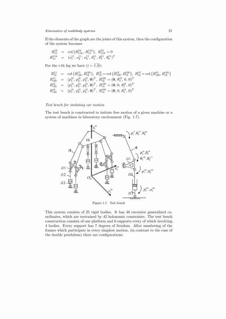
Figure 1.7. Test bench
This system consists of 25 rigid bodies. It has 48 excessive generalized co-ordinates, which are restrained by 42 holonomic constraints. The test benchconstruction consists of one platform and 6 supports every of which involving4 bodies. Every support has 7 degrees of freedom. After numbering of theframes which participate in every simplest motion, (in contrast to the case ofthe double pendulum) there are configurations:

22 Chapter 1
- for the platform
R1011 = col R1011k, R11k11 , R1011k = 0, R11k11 = (o111 , 0, 0, 0)T
R1112 = col R1112k, R12k12 , R1112k = 0, R12k12 = (0, o122 , 0, 0)T
R1213 = col R1213k, R13k13 , R1213k = 0, R13k13 = (0, 0, o133 , 0)T
R1314 = col R1314k, R14k14 , R1314k = 0, R14k14 = (0, θ144 , 0, 0)T
R1415 = col R1415k, R15k15 , R1415k = 0, R15k15 = (0, 0, θ155 , 0)T
R1516 = col R1516k, R16k16 , R1516k = 0, R16k16 = (0, 0, 0, θ166 )T
- for i-th support (i = 1, 6)
R16i7 = col R16i7k, Ri7ki7 , R16i7k = (pi71 , pi72 , pi73 , 0)T
Ri7ki7 = (0, θi74 , 0, 0)T , Ri7i8 = col Ri7i8k, Ri8ki8 , Ri7i8k = 0
R18ki8 = (0, 0, 0, θi86 )T , Ri8i9 = col Ri8i9k, Ri9ki9 , Ri8i9k = (0, pi92 , 0,0)T
Ri9ki9 = (0, θi94 , 0, 0)T , Ri9i10 = col Ri9i10k, Ri10ki10 , Ri9i10k = 0
Ri10ki10 = (0, 0, θi105 , 0)T , Ri10i11 = col Ri10i11k, Ri11ki11 , Ri10i11k = 0Ri11ki11 = (0, 0, 0, θi116 )T , Ri11i12 = col Ri11i11k, Ri11ki12 Ri11i11k = (0, pi122 , 0, 0)T , Ri11ki12 = (0, 0, 0, θi126 )T
Ri12i13 = col Ri12i13k, Ri13ki13 , Ri12i13k = (0, pi132 , 0, 0)T
Ri13ki13 = (0, oi132 , 0, 0)T
1.3. Kinematic equations of (µ, k − 1; lk)-th kinematic pair
Kinematic equations give the connection between the coordinates of twist of(µ, k− 1; lk)-th kinematic pair and the generalized coordinates and velocitiesof this pair. Let us begin with deriving the main kinematic equalities of thistheory (Gantmacher 1964, Diedonne 1972, Konoplev 1986b, Velichenko 1988).To establish them we need the following notion.
Definition 1.9 Let Wστ = col wστ , vστ be the twist of motion of the frame
Eτ with respect to Eσ. Then the vector
V στ = col vστ , wστ
is called the quasi-velocity of Eτ with respect to Eσ.
Proposition 1.16 Let
− Ek take part in a motion with respect to Es, and Ep take part in amotion with respect to Ek;− W s
k , Wkp , W
sp be the twists of the kinematic pairs (Es, Ek), (Ek, Ep)
and (Es, Ep) (see (1.20), (1.21)).

Kinematics of multibody systems 23
Then the following kinematic equalities hold
W spp = LpkW
skk +W kp
p , Vspp = Lk,Tp V skk + V kpp (1.28)
where
− Lpk is a motion from group (1.15);− W sk
k , Wkpp , W
spp and V skk , V kpp , V spp are the coordinate representations
of the twists and the corresponding quasi-velocities.
Proof 1. After reducing all twists to Ep, we get that Wsppp = W
spkp +W
kppp .
After that, to prove the first equality it is enough to apply transform (1.13). 2.To prove the second equality, let us introduce 6×6-dimensional matrix ² whosemain diagonal is formed by two 3 × 3-dimensional null matrixes, and whosesecond diagonal is formed by two 3× 3-dimensional identity matrixes. Since²² = E: we get easily that ²W sp
p = ²Lpk²²Wskk + ²W kp
p where ²Lpk² = Lk,Tp . 2
The term main emphasizes the fundamental meaning of equality (1.28): thederiving of the kinematic equations for subsystems of the basic system is doingwith its help.
Proposition 1.17 (Konoplev 1984 and 1986b,c) Let
− the configuration of the pair (µ, k − 1; lk) be given by relation (1.24);− Lµ,k−1lk = Lµ,k−1lkk Llkklk be a transformation of the coordinate columns ofscrews, generated by configuration (1.24), where the transformation
Lµ,k−1lkk = Tµ,k−1lkk Cµ,k−1lkk
is defined by the constructive configuration
Rµ,k−1lkk = col pµ,k−1lkk , φµ,k−1lkk pµ,k−1lkk ≡ pµ,k−1;µ,k−1lk , φµ,k−1lkk ≡ φµ,k−1lk
and the transformation Llkklk = T lkklk Clkklk is induced by the functional
configuration Rlkklk = col 0, . . . , 0, qlki , 0, . . . , 0:
Tµ,k−1lkk =
·E O
pµ,k−1lkk E
¸, Cµ,k−1lkk = diag cµ,k−1lkk , cµ,k−1lkk
cµ,k−1lkk = cα−3(φlkα )cβ−3(φlkβ )cγ−3(φ
lkγ )
ci−3(φlki ) = E + elki−3 sinφlki + e
lki−3(1− cosφlki )2
Llkklk =
½T lkklk if i = 1, 3Clkklk otherwise
T lkklk =
·E Oolkklk E
¸, Clkklk = diag clkklk , clkklk
olkklk = col 0, . . . 0, olki , 0, . . . 0, clkklk = ci(θlki+3), i = 1, 3

24 Chapter 1
Then the kinematic equation of (µ, k − 1; lk)-th kinematic pair is
V µ,k−1;lklk = Rlkk.lk = f lki qlk.i , q
lk.i =
½olk.i if i = 1, 3θlk.i if i = 4, 6
(1.29)
where f lki is 6-dimensional (unit) column such that its i-th entry is equal to 1(i = 1, 6), the other ones are equal to zero.
Proof In order to simplify the proof let us re-number by the integers0, 1, . . . , 7 the frames that participate in every simplest constructive and func-tional motions of (µ, k − 1; lk)-th kinematic pair. Hence, the motion of(µ, k − 1; lk)-th kinematic pair will be a superposition of the simplest mo-tions E0 → E1 → . . . → E7, E0 = Eµ,k−1, E7 = Elk, and the first six ofthem p11, p
22, p
33, φ
4α, φ
5β, and φ
6γ are constructive, while the 7-th q
7i , i = 1, 6,
is functional.From the second equation of (1.28) follows that
V µ,k−1;lklk = V 077 = L1,T7 V 011 + V 177 = L1,T7 V 011 + L2,T7 V 122 + V 277 =
L1,T7 V 011 + L2,T7 V 122 + L3,T7 V 2,33 + L4,T7 V 344 + L5,T7 V 455 +
L6,T7 V 566 + L7,T7 V 677 V677 ; V
066 = 0
V 677 =
½col c6,T7 e7i o
7.i ;0
T = col e7i o7.i ,0T if i = 1, 3col 0T , e7i θ7.i otherwise
and finally V µ,k−1;lklk = col v677 , w677 = f7i q7.i = f lki q
lk.i due to V n,n+1n+1 =
0, n = 0, 5. 2
Let the configuration of (µ, k − 1; lk)-th kinematic pair be given in the form(1.24)-(1.27).
Notation 1.8 Henceforth
− Lµ,k−1lk = Lµ,k−1lkk Llkklk is transformation of the coordinates of twists in-
duced by the configuration Rµ,k−1lk = col Rµ,k−1lkk , Rlkklk where the trans-formation Lµ,k−1lkk = Tµ,k−1lkk Cµ,k−1lkk is determined by the constructive con-
figuration Rµ,k−1lkk = col plk, φlk and the transformation Llkklk = T lkklk Clkklkis determined by the functional one Rlkklk = col olk, θlk;− qlk is the column of generalized coordinates of (µ, k−1; lk) -th kinematicpair (non-null elements of the functional configuration Rlkklk );− ²lkklk is 3× 3-dimensional matrix of the kind
²lkklk = kcT3 (θlk6 )cT2 (θlk5 )elk1 | cT3 (θlk6 )elk2 | elk3 k− clkklk = c1(θ
lk4 )c2(θ
lk5 )c3(θ
lk6 ) be the orientation matrix for e
lk in theconstructive frame Elkk;
M lkklk = diag clkk,Tlk , ²lkklk (1.30)

Kinematics of multibody systems 25
is the matrix of transition from the generalized velocities qlk.i of (µ, k −1; lk)-th kinematic pair to the quasi-velocities V µ,k−1;lklk of the same kine-matic pair.
Proposition 1.18 (Konoplev 1984 and 1986b,c) The kinematic equation of(µ, k − 1; lk)-th kinematic pair is
V µ,k−1;lklk =M lkklk R
lkk.lk =M lkk
lk kf lkkqlk. (1.31)
where kf lkk is the mobility axes matrix for (µ, k−1; lk)-th kinematic pair thatis constituted by the 6-dimensional unit columns f lki (each of them has 1 atits i-th position, i = 1, 6, the other ones being equal to zero).
Proof As in the previous case, to simplify the proof let us re-number bythe integers 0, 1, . . . , 12, the frames that participate in the simplest con-structive and functional motions of (µ, k − 1; lk)-th kinematic pair. Thenmotion of (µ, k − 1; lk)-th kinematic pair will be superposition of twelve sim-plest motions E0, E1, E2, . . . , E12, where E0 = Eµ,k−1, E12 = Elk, thefirst six of them p11, p
22, p
33, φ
4α, φ
5β and φ6γ are constructive and the second
six o71, o82, o
93, θ
104 , θ
115 and θ126 are functional. Taking in account the second
equality from (1.28) we obtain
V µ,k−1,klk = V 0,1212 = L1,T12 V011 + L2,T12 V
122 + L6,T12 V
566 + L7,T12 V
677 +
L8,T12 V788 + L9,T12 V
899 + L10,T12 V 9,1010 + L11,T12 V 10,1111 +
L12,T12 V 11,1212 = L7,T12 col v677 ,0T + L8,T12 col v788 ,0T +
L9,T12 col v899 ,0T + L10,T12 col 0T , w9,1010 +
L11,T12 col 0T , w10,1111 + L12,T12 col 0T , w11,1212 =C7,T12 T
7,T12 col v677 ,0T + C
8,T12 T
8,T12 col v788 ,0T+
C9,T12 col v899 ,0T+ C10,T12 col 0T , w9,1010 +
C11,T12 col 0T , w10,1111 + col 0T , w11,1212 =col 0T , c11,T12 c10,T11 w9,1010 + C10,T12 col v697 + v798 + v899 ,0
T+col 0T , c11,T12 w10,1111 + col 0T , w11,1212 =col c9,T12 v699 ,0T + col 0T , c
11,T12 c10,T11 e101 θ10.4 +
col 0T , c11,T12 e112 θ11.5 + col 0T , e123 θ12.6 =col 0T , ²912col θ10.4 , θ11.5 , θ12.6 + col c9,T12 v699 ,0T =col c6,T12 col o7.1 , o8.2 , o9.3 ,0T +col 0T , ²612col θ10.4 , θ11.5 , θ12.6 =M612(o
71, o
82, o
93, θ
10.4 , θ11.5 , θ12.6 )T =M lkk
lk kf lkkqlk. 2

26 Chapter 1
1.3.1. Examples of equations of kinematic pairs
Gyroscope (Fig. 1.2)
There are
V 011 = M1k1 f
14 θ1.4 = Ef
14 θ1.4 , V
122 =M2k
2 f25 θ2.5 = f
25 θ2.5
V 233 = M3k3 f
36 θ3.6 = f
26 θ3.6
Flywheel (Fig. 1.3)
There is
V 0ss = fs6θs.6
Double pendulum (Fig. 1.4)
There are two variants to write down the equations. The first one is
V 011 = M1k1 f
12 o1.2 = f
12 o1.2 , V
122 =M2k
2 f25 θ2.5 = f
25 θ2.5
V 233 = M3k3 f
36 θ3.6 = f
36 θ3.6
And the second variant is
V 011 = kf12 | f15 kcol o1.2 , θ1.5 = kf1kq1., kf1k = kf12 | f15 kV 122 = M2k
2 f25 θ2.5 = f
36 θ3.6 , q
1. = col o1.2 , θ1.5 , q2.6 = θ3.6
Manipulator (Fig. 1.5)
There are
V 011 = M1k1 f
14 θ1.4 = f
14 θ1.4 , V
122 =M2k
2 f25 θ2.5 = f
25 θ2.5 , . . . ,
V 566 = M6k6 f
66 θ6.6 = f
66 θ6.6
Walking machine (Fig. 1.6)
There is
V 10,1111 =M11k11 kf11kq11.
where for the matrix M11k11 we get
c11k,T11 = cT3 (θ116 )c
T2 (θ
115 )c
T1 (θ
114 )
²11k11 = kcT3 (θ116 )cT2 (θ115 )e111 | cT3 (θ116 )e112 | e113 kf11 = E, q11 = (o111 , o
112 , o
113 , θ
114 , θ
115 , θ
116 )
T
V 11,i2i2 = M i2ki2 f
i24 θi2.4 = f i24 θi2.4 , . . . , V
i3,i4i4 =M i4k
i4 fi45 θi4.5 = f i45 θi4.5

Kinematics of multibody systems 27
Test bench (Fig. 1.7)
For the platform from variant 1 is fulfilled that
V 10,1111 =M11k11 f
111 o
11.1 = f111 o
11.1 , . . . , V 15,1616 =M16k
16 f166 θ16.6 = f116 θ16.6
For the platform from variant 2 (by analogy with the previous system) isfulfilled that
V 10,1111 =M11k11 kf11kq11.
where in the matrix M11k11 we get
c11k,T11 = cT3 (θ116 )c
T2 (θ
115 )c
T1 (θ
114 )
²11 = kcT3 (θ116 )cT2 (θ115 )e111 | cT3 (θ116 )e112 | e113 kkf11k = E, q11 = (o111 , o
112 , o
113 , θ
114 , θ
115 , θ
116 )
T
For i-th support there are
V 16,i7i7 = f i74 θi7.4 , Vi7,i8i8 = f i86 θi8.6 , V
i9,i9i9 = f i94 θi9.4
V i9,i10i10 = f i10θi105 , . . . , V i12,i13i13 = f i132 oi13.2
1.4. Kinematics of Hooke-elastic pair
Let us introduce the definition of an elastic pair.
Definition 1.10 The kinematic pair (µ, k − 1; lk) is called an elastic one if− Rµ,k−1lkk = (plk1 , p
lk2 , p
lk3 ,φ
lkα ,φ
lkβ ,φ
lkγ )
T is its constructive configuration;
− Rlkklk = (olk1 , olk2 , o
lk3 , θ
lk4 , θ
lk5 , θ
lk6 )
T is its functional configuration;− col δlk1 , δlk2 , δlk3 is the column of linear distortions of (µ, k − 1)-th ele-ment of the system;− col δlk4 , δlk5 , δlk6 is the column of angular deformations of (µ, k − 1)-thelement of the system;− δlki 6= 0, if olki = 0 or θlki = 0, and δlki = 0, if olki 6= 0 or θlki 6= 0,or δlki = olki = θlki = 0, if functional motions of arbitrary origin are notencountered in i-th coordinate of the pair.
From the above definition conditions follows that the elements of the elasticpair (µ, k − 1; lk) are rigid bodies. It is easy to see that configuration (1.27)of the elastic pair (µ, k − 1; lk) assumes form (1.24) where (Konoplev 1986b,Konoplev et al. 1991)
Rµ,k−1lkk = col plk,φlk, Rlkklk = (δlk1 , δlk2 , δ
lk3 , δ
lk4 , δ
lk5 , δ
lk6 )
T +
(olk1 , olk2 , o
lk3 , θ
lk4 , θ
lk5 , θ
lk6 )
T = col qlki
and qlki is equal to olki , or θlki , or δ
lki , or 0.

28 Chapter 1
Proposition 1.19 Kinematic equations of the elastic pair (µ, k − 1; lk) as-sume the following form
V µ,k−1;lklk =M lkklk kf lkkqlk. (1.32)
where M lkklk is defined by relation (1.31) with the matrices
clkklk = c1(qlk4 )c2(q
lk5 )c3(q
lk6 )
²lkklk = kcT3 (qlk6 )cT2 (qlk5 )elk1 | cT3 (qlk6 )elk2 | elk3 k (1.33)
The transference of lk-th body with respect to Elkk is realized on account ofthe functional motions (deformations of (µ, k−1)-th element) which can haveboth elastic and non-elastic character (here, the influence of the first ones onthe one-index seconds is neglected).
Example
Let us consider an one-joint pendulum (see fig. 1.4) (or more precisely, the lastarm of the double pendulum) within the framework of the assumption thatfirst two generalized coordinates have elastic character. Due to our previouspropositions we obtain that
R01 = col R01k, R1k1 , R01k = 0, R1k1 = (0, δ12 , 0,0)T
R12 = col R12k, R2k2 , R12k = 0, R2k2 = (0, 0, δ25 , 0)T ,
R23 = col R23k, R3k3 , R23k = (p31, 0, 0,0)T , R3k3 = (0, 0, 0, θ36)T
V 011 = M1k1 f
12 δ1.2 = f
12 δ1.2 , V
122 =M2k
2 f25 δ2.5 = f
25 δ2.5
V 233 = M3k3 f
36 θ3.6 = f
36 θ3.6
V 011 = kf12 | f15 kq1. = kf1kq1., V 122 =M2k2 f
25 θ2.5 = f
36 θ3.6
f1 = kf12 | f15 k, q1. = col δ1.2 , δ1.5 , q2.6 = θ3.6
Proposition 1.20 In the study of elastic systems of rigid bodies the use ofconfigurations of the (1.24)-kind is not allowable.
The proof of this proposition will be given in Chapter 2.

Kinematics of multibody systems 29
1.5. Kinematic equations of lk-th element
Equations of kinematics of lk-th element of the system give a connectionbetween the quasi-velocities of the kinematic pairs of (10, lk)-th kinematic
chain and the quasi-velocity column V 10,lklk of lk-th element in E10.
Proposition 1.21 (Konoplev 1989b,c and 1990) Let
1. V i,j−1;njnj = col vi,j−1;njnj , wi,j−1;njnj be the quasi-velocity columns of allkinematic pairs from the set (lk)−of counter accessibility for lk-th elementof the system (of some body or frame that takes part in some of the simplestfunctional motions);
2. Ri,j−1nj = col Ri,j−1njk , Rniknj be configurations of all kinematic pairs from(lk)− defined by (1.25) and (1.26) or (1.27);
3. Li,j−1nj = Li,j−1njk Lniknj be the motion of linear spaces of twists of all kine-
matic pairs from (lk)− that corresponds to the configuration Ri,j−1nj from
condition 3 (see (1.13));
4. Lnjlk = Lnjm,j+1Lm,j+1g,j+2 . . . L
d,k−1lk be the composition of motions from con-
dition 4 taken for all elements of lk-th kinematic chain from intersectionof the sets of accessibility and counter accessibility for the (nj)- and (lk)-elements of the system, respectively.
Then the kinematic equation of lk-th element of the system in the main frameE10 has the following form
V 10,lklk =X
nj∈(lk)−Lnj,Tlk V i,j−1;njnj (1.34)
where the right-hand side is represented as the linear combination of thecolumns V i,j−1;njnj with the matrix coefficients Lnj,Tlk .
Proof To simplify notations let us consider a kinematic chain (a tree withonly one stem), which permits us to turn to one position number indices.Using (1.28) we obtain
V 0,kk = L1,Tk V 0,11 + V 1,kk = L1,Tk V 0,11 + L2,Tk V 1,22 + V 2,kk = L1,Tk V 0,11 +
L2,Tk V 1,22 + L3,Tk V 2,33 + . . .+ V l−1,kk =kXp=1
Lp,Tk V p−1,pp
where Lpk = Lpp+1L
p+1p+2 . . . L
k−1k . 2
Taking in account the kinematic equations of kinematic pairs (1.32) and (1.33),we may write equation (1.34) in another form.
Proposition 1.22 Let
− (lk)− be (10, lk)-th kinematic chain;

30 Chapter 1
− (i, t− 1; st) be a kinematic pair of the (1.24)-kind andsst−αlk = fst,Tα Mstk,T
st Lstlk (1.35)
be 6-dimensional row-operator of projection of the binary vector X lklk
(given in Elk) without regard to its origin (kinematic, dynamic, kinetic,etc.) on the α-axis of the functional motion of st-th element of the systemin (i, t− 1; st)-th kinematic pair, α = 1, 6;− (i, t− 1; st) be a kinematic pair of the (1.27)-kind and
sstlk = col fst,Tα Mstk,Tst Lstlk = kfstkTMstk,T
st Lstlk (1.36)
be (vdim qst)×6-dimensional matrix of projection of the binary vector X lklk
(given in Elk) without regard to its origin (kinematic, dynamic, kinetic,etc.) to the axis of the functional motion of st-th element of the systemin (i, t − 1; st)-th kinematic pair, α = 1, 6, where kfstk is the matrix ofthe unit columns fstα .
Then
− there is the kinematic equation of lk-th element of the system in theframe E10
V 10,lklk =X
nj∈(lk)−snj−α,Tlk qnj.α (1.37)
where the right-hand side is represented as the linear combination ofcolumns of the generalized velocities qnj.α , α = 1, 6, of lk-th elements
of the kinematic chain with 6 -dimensional column-coefficients snj−α,Tlk
for kinematic pairs of the (1.24)-(1.26)-kind;− there is the kinematic equation of lk-th element of the system in theframe E10
V 10,lklk =X
nj∈(lk)−snj,Tlk qnj.α (1.38)
where the right-hand side is represented as the linear combination ofcolumns of generalized velocities qnj. of lk-th elements of the kinematicchain with 6× (vdim qnj.)-dimensional matrix coefficients snj,Tlk for kine-matic pairs of the (1.27)-kind.
Proof The proof is easily produced with the help of substitution in (1.34)the corresponding quantities from (1.32) and (1.33) (due to (1.37) and (1.38),e.g.:
V 10,lklk =X
nj∈(lk)−Lnj,Tlk V i,j−1;njnj =
Xnj∈(lk)−
Lnj,Tlk Mnjknj kfnjkqnj. =
Xnj∈(lk)−
sni,Tlk qnj. 2

Kinematics of multibody systems 31
1.5.1. Examples of kinematic equations of kinematic pairs
Gyroscope (Fig. 1.2)
There are
V 011 = f14 θ1.4 = s
1−4,T1 θ1.4
V 022 = L1,T2 V 011 + V 122 = L1,T2 f14 θ1.4 + f
25 θ2.5 = s
1−4,T2 θ1.4 + s
2−5,T2 θ2.5
V 033 = L1,T3 V 011 + L2,T3 V 122 + L3,T3 V 233 = L1,T3 f14 θ1.4 + L
2,T3 f25 θ
2.5 +
Ef36 θ3.6 = s
1−4,T3 θ1.4 + s
2−5,T3 θ2.5 + s
3−6,T3 θ3.6
s1−4,T1 = f14 , s1−4,T2 = L1,T2 f14 , s
1−4,T3 = L1,T3 f14 , s
2−5,T2 = f25
s2−5,T3 = L2,T3 f25 , s3−6,T3 = f36 , L
12 = L
12kL
2k2 = L2k2 = C2(θ
25)
L13 = L12L23, L
23 = L
23kL
3k3 = L3k3 = C3(θ
36)
Double pendulum (Fig. 1.4)
In the case of variant 1 there are
V 011 = f12 o1.2 = s
1−2,T1 o1.2
V 022 = L1,T2 V 011 + V 122 = L1,T2 f12 o1.2 + f
25 θ2.5 = s
1−2,T2 o1.2 + s
2−5,T2 θ2.5
V 033 = L1,T3 V 011 + L2,T3 V 122 + L3,T3 V 232 = L1,T3 f12 o1.2 + L
2,T3 f25 θ
2.5 +
f36 θ3.6 = s
1−2,T3 o1.2 + s
2−5,T3 θ2.5 + s
3−5,T3 θ3.6
s1−2,T1 = f12 , s1−2,T2 = L1,T2 f12 , s
2−6,T3 = L1,T3 f12
L12 = L12kL2k2 = C2(θ
25), L
23 = L
23kL
3k3 , L
13 = L
12L
23 = T
23kC3(θ
36)
where the matrix T 23k is induced by the column of constructive translationp3 = col p31, 0, 0 (see Section 1.3.1).In the case of variant 2 there are
V 011 = kf12 , f15 kcol o1.2 , θ1.5 = kf1kq1. = s1,T1 q1.
V 022 = L1,T2 V 011 + V 122 = L1,T2 kf1kq1. + f26 θ2.5 = s1,T2 q1. + s2−6,T2 θ2.6
s1,T1 = kf1k, s1,T2 = L1,T2 kf1k, s2−6,T2 = f26L12 = L12kL
2k2 = C3(θ
26) = T
12kC3(θ
26)
where the matrix T 12k is induced by the column of constructive translationp2 = col p21, 0, 0 (see Section 1.3.1).
Manipulator (Fig. 1.5)
There are
V 011 = f12 θ1.4 = s
1−4,T1 θ1.4

32 Chapter 1
V 022 = L1,T2 V 011 + V 122 = L1,T2 s1−4,T1 θ1.4 + f25 θ2.5 =
s1−4,T2 θ1.4 + s2−5,T2 θ2.5
V 033 = L1,T3 V 011 + L2,T3 V 122 + V 233 = s1−4,T3 θ1.4 +
s2−5,T3 θ2.5 + s3−5,T3 θ3.5
. . . . . . . . . . . . . . . . . . . . . . . . . . . . . . . . . . . . . . . . . .
V 066 = L1,T6 V 011 + L2,T6 V 122 + . . .+ V 566 = s1−4,T6 θ1.4 + s2−5,T6 θ2.5 +
s3−5,T6 θ3.5 + . . .+ s6−6,T6 θ6.6
s1−4,T6 = L1,T6 f14 , s2−5,T6 = L2,T6 f25 , . . . , s
6−6,T6 = f66
L16 = L12L23L
34L
45L
56, L
12 = L
12kL
2k2 = C2(θ
25)
L23 = L23kL3k3 = T 23kC2(θ
35), L
34 = L
33kL
3k4 = T 33kC1(θ
44), . . . ,
L56 = L56kL6k6 = T 56kC3(θ
66) = C3(θ
66)
where the matrices T 23k, T33k are induced by the columns of constructive trans-
lations p3 = col 0, p32, 0, p4 = col 0, p42, 0.
Walking machine (Fig. 1.6)
There are
V 10,1111 = M11k11 kf11kq11. = s
11,T11 q11.
V 10,i2i2 = L11,Ti2 V 10,1111 + V 10,i2i2 = L11,Ti2 M11k11 kf11kq11. +
f i2.4 θi2.4 = s11,Ti2 q11. + si2−4,Ti2 θi2.4
V 10,i3i3 = L11,Ti3 V 10,1111 + Li2,Ti3 V 11,i2i2 + V 12,i3i3 =
s11,Ti3 q11. + si2−4,Ti3 θi2.4 + si3−4,T.i3 θi3.5
V 10,i3i4 = s11,Ti4 q11. + si2−4,Ti4 θi2.4 + si3−5,T.i4 θi3.5 + si4−5,Ti4 θi4.5
Test bench (Fig. 1.7)
In the case of variant 1, for the platform there are
V 10,1111 = s11−1,T11 o11.1 , V 10,1212 = s11−1,T12 o11.1 + s12−2,T12 o11.2 , . . . ,
V 10,1616 = s11−1,T16 o11.1 + s12−2,T16 o12.2 + s13−3,T16 o13.3 + s14−4,T16 o14.4 +
s15−5,T16 o15.5 + s16−6,T16 o16.6 = S11,Ti6 q11.
For i-th support there are
V 10,i7i7 = S11,Ti7 q11. + si7−4,Ti7 θi7.4
V 10,i8i8 = S11,Ti8 q11. + si7−4,Ti8 θi7.4 + si8−6,Ti8 θi8.6
Kinematics of multibody systems 33
V 10,i9i9 = S11,Ti9 q11. + si7−4,Ti9 θi7.4 + si8−6,Ti9 θi8.6 + si9−4,Ti9 θi9.4
V 10,i10i10 = S11,Ti10 q11. + si7−4,Ti10 θi7.4 + si8−6,Ti10 θi8.6 +
si9−4,Ti10 θi9.4 + si10−5,Ti10 θi10.5
V 10,i13i13 = S11,Ti13 q11. + si7−4,Ti13 θi7.4 + si8−6,Ti13 θi8.6 + si9−4,Ti13 θi9.4 +
si10−5,Ti13 θi10.5 + si11−6,Ti13 θi11.6 + si12−6,Ti13 θi12.6 + si13−2,Ti13 θi13.2
where
S11,Tij = ks11−1,Tij | s12−2,Tij | s13−3,Tij | s14−4,Tij | s15−5,Tij | s16−6,Tij k
are the matrices (j = 6, 13) standing before the rows q11., the matrix S11,T16
being the same as the matrix s11,T11 from the previous example.
1.6. Kinematic equations of a tree-like multibody system
Let (10)+ be a multibody system with tree-like structure. We shall givekinematic equations in several forms (Konoplev 1989a and 1990).
Notation 1.9 Henceforth
− V = col V i,j−1;njnj is 6n-dimensional quasi-velocity column of kine-matic pairs of the system (see (1.29), (1.31)) (recall that n is the numberof rigid bodies of the system);
− V = col V 10,lklk is 6n-dimensional quasi-velocity column of lk-th ele-ments of the system (see (1.37), (1.38));− L is an upper-triangular block 6n× 6n-dimensional matrix with 6× 6-dimensional matrix blocks Lstlk (see Proposition 1.21, condition 5) if (lk) ∈(st)+ and with 6× 6-dimensional null matrix blocks if (lk) /∈ (st)+, Lstlkstanding at the place of intersection of st-th row and lk-th column.
Proposition 1.23 The kinematic equations of the system with tree-like struc-ture have the form
V = LT V (1.39)
where L is called a configuration matrix of the system.
The proof of this statement can be produced simply by writing down matrixform of equations (1.34) for lk-th element of the system. The reason for sucha name of the matrix L is the fact that its elements contain all informationabout the configuration of the system (except the configuration R1011).
Let us now find the relation between the column V and that of the generalizedvelocities of the system.

34 Chapter 1
Proposition 1.24 The relation between the column V and that of the gener-alized velocities of the system (see (1.29), (1.31)) assumes the following form
V =MFq· (1.40)
where− M is the block-diagonal 6n× 6n-dimensional matrix of transition fromgeneralized velocities of the multibody system to quasi-velocities of theirkinematic pairs (see (1.30))
M = diag M lkklk
− F is the block-diagonal matrix, whose blocks on the main diagonal arethe 6 × (vdim qlk.)-dimensional blocks kf lkk composed by 6-dimensionalunit coordinate columns f lki , (i = 1, 6), of the mobility axes of the kine-matic pairs
F = diag kf lkk− q· = col qlk. is the column of generalized velocities of the system,which is composed by columns of generalized velocities of kinematic pairsof the system.
Proof Equality (1.40) is just matrix representation of kinematic equationsof the all kinematic pairs of the multibody system. 2
From relations (1.39) and (1.40) we get the final form of the kinematic equa-tions of the tree-like system of bodies.
Proposition 1.25 The kinematic equations of the tree-like system are
V = ST q· (1.41)
where
S = FTMTL (1.42)
Note that S is (vdim qst)× 6n-dimensional upper triangular matrix with theblocks
sstlk = col sst−αlk (1.43)
at the intersection of (vdim qst)×6n-dimensional matrix row and (vdim q)×6-dimensional matrix column in the case of (lk) ∈ (st)+, and with the null blockat this position in the case of (lk) /∈ (st)+. Here s
st−αlk = fst,Tα Mstk,T
st Lstlk are 6-
dimensional rows being operators of projection of the binary vector X lklk given
in Elk, which can be of arbitrary origin (kinematic, dynamic, kinetic, etc.),on the α-axis of the functional motion of st-th element from (i, t − 1; st)-thkinematic pair, α = 1, 6 (see (1.35), (1.36)).
We may obtain the proof with substituting the relation (1.40) in (1.39) andafter that with multiplying the matrices FT ,MT and L by hand and takinginto account (1.43).

Kinematics of multibody systems 35
Definition 1.11 The matrix S is called parastrophic matrix for the tree-likesystem of bodies.
In the mechanical formalism developed here, the parastrophic matrix S playscentral role. Its name is inspired by the reason that it brings full informationabout the structure of system of bodies, namely, about:
− inner configuration of the system and the structure of kinematic schemeof the system, with the help of the matrix L;
− transition from quasi-coordinates of system to generalized coordinates ofthe system with the help of the matrixM;
− character of motion in respect to any one of the degrees of freedom,for which stands the matrix F which is composed by 6-dimensional unitcolumns (along the directions of motions of the system).
The physical meaning of the matrix S is clear: S projects the 6n-dimensionalcolumn P = col P lklk of binary vectors of arbitrary origin on the axes of mo-tion of the system. The matrix ST produces the inverse operation: it trans-forms the generalized velocities of the system into the quasi-velocity columns(1.41) (in the twists).
Above the theory of constructing the parastrophic matrix is considered indetail. The concluding algorithm for constructing it (numerically or symboli-cally) is presented by the three next procedures (the content of which dependson the choice of indices):
− the matrices sstst that constitute the main diagonal of (1.43) are formedby the relationsstst = kfstkTM
stk,Tst
In the case of using configuration (1.24), there are no computational ex-penditure assst−αst = fst,Tα Mstk,T
st ≡ fst,Tα
− the matrices Lµ,k−1lk of all kinematic pairs (µ, k− 1; lk) of the system areformed according toLµ,k−1lk = Lµ,k−1lkk Llkklk
− (st)-rows of the matrices sstlk are formed with starting from sstν,t+1 by therelationsstlk = s
stµ,k−1L
µ,k−1lk
1.6.1. Examples of constructing configuration matrices
Gyroscope on a tilted base and double pendulum (Fig. 1.2)
There are
V = col V 011 , V 022 , V 032
V = col V 011 , V 122 , V 233 , L =
E L12 L13O E L23O O E

36 Chapter 1
Manipulator (Fig. 1.5)
There are
V = col V 011 , V 022 , V 033 , . . . , V 066
V = col V 011 , V 122 , V 233 , . . . , V 566 , L =
E L12 L13 . L16O E L23 . L26. . . . .O O O . E
Walking machine (Fig. 1.6)
There are
V = col V 10,1111 , V 10,1212 , V 10,1313 , V 10,1414 , V 10,2222 , V 10,2323 , V 10,2424 , . . . ,
V 10,6262 , V 10,6363 , V 10,6464 V = col V 10,1111 , V 11,1212 , V 12,1313 , V 13,1414 , V 11,2222 , V 22,2323 , V 23,2424 , . . . ,
V 11,6262 , V 62,6363 , V 63,6464
L =
E L1112 L1113 L1114 L1122 L1123 L1124 . L1162 L1163 L1164O E L1213 L1214 O O O . O O OO O E L1314 O O O . O O OO O O E O O O . O O OO O O O E L2223 L2224 . O O OO O O O O E L2324 . O O OO O O O O O E . O O O. . . . . . . . . . .O O O O O O O . E L6263 L6264O O O O O O O . O E L6364O O O O O O O . O O E
The number of non-null 6× 6-dimensional blocks used above is 55.
Test bench (Fig. 1.7)
There are
V = col V 10,1111 , V 10,1212 , . . . , V 10,1616 , V 10,1717 , V 10,1818 , V 10,1919 , V 10,110110 , . . . ,
V 10,113113 , . . . , V 10,6767 , V 10,6868 , V 10,6969 , V 10,610610 , . . . , V 10,613613 V = col V 10,1111 , V 11,1212 , . . . , V 15,1616 , V 16,1717 , V 17,1818 , V 18,1919 , V 19,110110 , . . . ,
V 112,113113 , . . . , V 16,6767 , V 67,6868 , V 68,6969 , V 69,610610 , . . . , V 612,613613

Kinematics of multibody systems 37
The matrix L has the following structure
L =
E ¦ ¦ ¦ ¦ ¦ ¦O ∗ O O O O OO O ∗ O O O OO O O ∗ O O OO O O O ∗ O OO O O O O ∗ OO O O O O O ∗
where 36 × 42 and 42 × 42-dimensional blocks ‘¦’ and ‘∗’ (respectively) areformed as in the previous example.
1.6.2. Examples of kinematic equations of kinematic pairs
Gyroscope (Fig. 1.2)
There is
M = diag E,E,E, F = diag f14 , f25 , f36 , q = col θ1.4 , θ2.5 , θ3.6
Double pendulum (Fig. 1.4)
In the case of variant 1 there is
M = E, F = diag f12 , f25 , f36 , q = col o1.2 , θ2.5 , θ3.6
In the case of variant 2 there are
F = diag kf1k, f36 , MF = F , q = col q1., θ3.6 kf1k = kf12 | f15 k, q1. = col o1.2 , θ1.5
Manipulator (Fig. 1.5)
There are
M = E, F = diag f14 , f25 , f35 , f44 , f55 , f66 ;q· = (θ1.4 , θ
2.5 , θ
3.5 , θ
4.4 , θ
5.5 , θ)
T
Walking machine (Fig. 1.6)
There are
M = diag M1011 , E,E, . . . , E

38 Chapter 1
F = diag E, f124 , f135 , f145 , f224 , f235 , f245 , f324 , f335 , f345 , f424 , f435 ,f445 , f
524 , f
535 , f
545 , f
624 , f
635 , f
645
q· = (q11., θ12.4 , θ13.5 , θ14.5 , θ22.4 , θ23.5 , θ24.5 , θ32.4 , θ33.5 , θ34.5 , θ42.4 ,
θ43.5 , θ44.5 , θ52.4 , θ53.5 , θ54.5 , θ62.4 , θ63.5 , θ64.5 )T
Test bench (Fig. 1.7)
There are
F = diag f111 , f122 , f13 f144 , f155 , f166 , f174 , f186 , f194 , f1105 , f1116 , f1126 ,
f1132 , f274 , f286 , f
294 , f
2105 , f2116 , f2126 , f2132 , f674 , . . . ,
f685 , f694 , f
6105 , f6116 , f6126 , f6132
q· = (o11.1 , θ17.4 , θ18.6 , θ19.4 , θ110.5 , θ111.6 , θ112.6 , o113.2 , θ27.4 , θ28.6 , θ29.4 , θ210.5 ,
θ211.6 , θ212.6 , o213.2 , . . . , θ67.4 , θ68.6 , θ9.4 , θ610.5 , θ611.6 , θ612.6 , o613.2 )T
1.6.3. Examples for constructing parastrophic matrices
Gyroscope (Fig. 1.2)
There is
S =
s1−41 s1−42 s1−43
O s2−52 s2−53
O O s3−63
1− 42− 53− 6
1 2 3
where
s1−41 = f1,T4 , s1−42 = f1,T4 L12, s1−43 = f1,T4 L13
s2−42 = f2,T5 , s2−53 = f2,T5 L23, s3−63 = f3,T6
Double pendulum (Fig. 1.4)
In the case of variant 1 there is
S =
s1−21 s1−22 s1−23
O s2−52 s2−53
O O s3−63
1− 22− 53− 6
1 2 3
(1.44)
where
s1−21 = f1,T2 , s1−22 = f1,T2 L12, s1−23 = f1,T2 L13
s2−52 = f2,T5 , s2−53 = f2,T5 L23, s3−63 = f3,T6

Kinematics of multibody systems 39
In the case of variant 2 there is
S =·s11 s12O s2−62
¸1
2− 61 2
where
s11 = kf1kT , s12 = kf1kTL12, s2−62 = f2,T6
Manipulator (Fig. 1.5)
There is
S =
s1−41 s1−42 s1−43 s1−44 s1−45 s1−46
O s2−52 s2−53 s2−54 s2−55 s2−56
O O s3−53 s3−54 s3−55 s3−56
O O O s4−44 s4−45 s4−46
O O O O s5−55 s5−56
O O O O O s6−66
1− 42− 53− 54− 45− 56− 6
1 2 3 4 5 6
where
s1−41 = f1,T4 , s1−42 = s1−41 L12, s1−43 = s1−42 L23
s1−44 = s1−43 L34, s1−45 = s1−44 L45, s
1−46 = s1−45 L56
Non-null elements of the other rows can be computed or constructed in thesimilar form by using analogous recurrent algorithms.
Walking machine (Fig. 1.6)
There is
S =
s1111 s1112 s1113 s1114 · s1162 s1163 s1164O f12,T4 s12−413 s12−414 · O O O
O O f13,T5 s13−514 · O O O
O O O f14,T5 · O O O· · · · · · · ·O O O O · f62,T4 s62−463 L62−464
O O O O · O f63,T5 s63−464
O O O O · O O f64,T5
1112− 413− 514− 5·
62− 463− 564− 5
11 12 13 14 · 62 63 64
where the number of 6 × 6-dimensional non-null blocks is 19 and of 3 × 6-dimensional non-null ones is 36.

40 Chapter 1
Test bench (Fig. 1.7)
Here the parastrophic matrix has the same structure as the matrix S fromthe previous example, but now the number and dimension of non-null blocksis different: here the number of 6 × 6-dimensional blocks is 49, of 3 × 6-dimensional ones is 240 and of 1× 6-dimensional ones is 48.
Amount of computational operations
Let us compute the amount of operations (N×/N+), that is necessary toconstruct the numerical form of the parastrophic matrix of a standard six-component arm with kinematic pairs having constructive translation alongone of the coordinates and also one functional rotation. The parastrophicmatrix of such system is upper triangular with blocks (1.43) in its upper-right
part. Its main diagonal consists of 6-dimensional unit columns f t,Ti , t = 1, 6,which are not to be computed. Above the main diagonal there are n(n−1)/2rows st−αk computed with the help of the relation
st−αk = st−αk−1Lk−1k , Lk−1k = Lk−1kk L
kkk
6-dimensional rows st−αk of the diagonal, which are situated above the main
diagonal of the matrix, are computed by selecting i-th row of the matrix T k−1kk
and subsequent multiplication to the matrix Ckkk . The maximal value of theworking time for such one operation is (2/0), and hence for the all matrixit will be (n − 1)2/0. For the 6-dimensional rows st−αk of the next diagonal(their number is n− 2) are required maximum (n− 2)4/2 operations, for the6-dimensional rows st−αk of the next diagonal are required at most (n− 3)8/4operations. For the any one from the other (n2 − n/2)− (n− 1)− (n− 2)−(n − 3) rows st−αk are necessary 10/6 operations (multiplication of the fullycompleted rows st−αk to T t−αkk Ckkk ). After summing up these results we obtainthat the maximal value of the working time of the algorithm for constructingthe parastrophic matrix is
N×(n) = 5n2 − 21n+ 26, (N×(6) = 80)N+(n) = 3n2 − 15n+ 20, (N+(6) = 38) (1.45)
For values of n less than 10, the presented estimation is overstated.
For example, the parastrophic matrix for the manipulator PUMA has only onerow s1−44 with estimation of the working time (10/4) and none with estimation(10/6) (see Section 1.6.3 - manipulator), which in the last three kinematicpairs is caused by the absence of constructive translations. With increasingn, the filling of the row st−αk increases also and estimation (1.45) of the workingtime tends asymptotically to the actual value.

Chapter 2
Equations of motion for a multibody system
2.1. Equations of motion of an element of a multibody system
Consider a system elements of which are rigid bodies, their motion beingassumed to be restricted by connections with other elements of the system(internal constraints) and also with bodies from the external environment(external constraints). In this chapter only holonomic internal constraintswill be regarded.
Notation 2.1 Henceforth− E0 is a frame with the origin O0 and the basis e0;− G is a body of the multibody system and Es is a frame attached to it(with the origin Os and the basis e
s);− xs is the radius vector of any point x ∈ G in Es, x
ss = col xss1 , xss2 , xss2 is its coordinate column in the basis es.
Proposition 2.1 The sliding vector lvs (in Es) (generated by the free vectorv(x) ≡ v0x of translation velocity of the point x with respect to E0) is the fol-lowing linear transformation of the linear (coordinate) space of quasi-velocitiesof the rigid body
lvss = ΘsxV0ss (2.1)
where V 0sss = V0ss = col v0ss , w0ss is the vector of quasi-velocities (in the basis
es) of Es with respect to E0 (see Definition 1.9); Θsx is 6 × 6-dimensional
matrix of the kind
Θsx =
·E −xssxss −xssxss
¸and (see (1.9))
xss =
0 −xss3 xss2xss3 0 −xss1−xss2 xss1 0
41

42 Chapter 2
Proof From w0ss xss = −xssw0ss = −xssw0ss follows that
lvss =
·E OO xss
¸µv0sxv0sx
¶=·
E OO xss
¸µv0ss + w0ss x
ss
v0ss + w0ss xss
¶=·
E −xssxss −xssxss
¸µv0sxw0sx
¶= ΘsxV
0ss
2
Proposition 2.2 The mass of G is defined by the integral
m(G) =
ZχGm(dx)
where χG is the characteristic function of points of D3 being occupied by G;m(dx) is a (Borel) mass measure.
Definition 2.1 We shall say that
− rsc = m−1(G)
ZχGx
sm(dx)
is the radius vector of the centroid of G in Es;− the point c ∈ G, settled in Es by the radius vector rsc , is the center ofgravity or also the centroid of G;− 3× 3-dimensional matrix
θss = −Z
χGxssxssm(dx) (2.2)
is the inertia matrix of the body G with respect to the point 0s (see sub-script) in the basis es (see superscript).
Notation 2.2 Henceforth
− 6×6-dimensional inertia matrices Θ00 and Θss (Mises ones) of the rigidbody G defined at the points 00 and 0s (the lower index) in the bases e
0
and es (the upper index) are defined in the form
Θkk =
·m(G)E −rkkc m(G)rkkc m(G) θkk
¸(2.3)
where k = 0 or k = s;− the integrals
Q00G0 =
ZχGl
v00 m(dx), Q0sGs =
ZχGl
vss m(dx) (2.4)
are the kinetic binary vectors in the motion of G in E0 with respect tothe frames E0 (see the inner indexes) and Es (see the outer indexes),respectively.
Equations of motion for a multibody system 43
Proposition 2.3 Let L0s ∈ L(R,6) be the transformation of the coordinatesof binary vectors that is induced by the motion Es → E0. Then
− the kinetic binary vector Q0sGs of G being in motion in Es taken withrespect to E0 is a linear transformation of the space of quasi-velocities ofG (Konoplev 1989a,c and 1990)
Q0sGs = ΘssV
0sss = Θ
ssV
0ss (2.5)
− the kinetic binary vectors Q00G0 and Q0sGs are connected by the followingrelation
Q00G0 = L0sQ
0sGs (2.6)
− the Mises matrices Θ00 and Θss are connected by
Θ00 = L0sΘ
ssL
0,Ts (2.7)
Proof 1. With the help of (2.1), (2.2) we obtain
Q0sGs =
ZχGl
vss m(dx) =
ZχGΘ
sxV
0sss m(dx) =Z
χGΘsxm(dx)V
0sss = Θ
ssV
0ss
2. Equation (2.6) is fulfilled due to the matrix L0s definition; 3. The proofof the equality Q00Gs = Θ
00V
00s0 is similar to the one in the proof beginning.
Because of (1.28), we get V 00s0 = Ls,T0 V 0sss and therefore Q00Gs = Θ00L
s,T0 V 0sss .
But from (2.5) and (2.6) follows that Q00G0 = L0sQ
0sGs = L
0sΘ
ssV
0ss . Therefore
Θ00Ls,T0 = L0sΘ
ss, and finally, taking in account (1.15), we obtain (2.7). 2
Henceforth we shall refer to binary vectors of reaction, friction and so on aswrenches (Murray et al. 1993) (sometimes the condition, that its componentsare parallell, is additionally included in the notion of a wrench, but we do notdemand it (see, e.g., Banach 1951, Targ 1976)). For the sake of brevity we in-troduce them with the help of integrals of the above kind (with correspondingdensities) without giving their formal definitions.
Notation 2.3 Henceforth
− the body Glk is an element of some tree-like system;− E10 is an inertial frame and Elk is a frame attached to Glk;− V 10,lklk = col v10,lklk , w10,lklk is the vector of quasi-velocities of Glk withrespect to E10 in Elk;− Θlklk is the Mises matrix of Glk in Elk (the constant matrix (2.3) iscalculated at the initial point Olk and in the basis e
lk of the frame attachedto the body);

44 Chapter 2
− Rlklk(i, k− 1; lk) and Rj,k+1j,k+1(lk; j, k+1) are wrenches of reactions of the
body Gi,k−1 ∈ (lk)− to the body Glk, and of the body Glk to the bodyGj,k+1 ∈ (lk)+, respectively,
Rlklk = Rlklk(i, k − 1; lk)−
Xj
Llkj,k+1Rj,k+1j,k+1(lk; j, k + 1) (2.8)
− N lklk (i, k − 1; lk) and N
j,k+1j,k+1 (lk; j, k + 1) are the wrenches of friction of
Gi,k−1 ∈ (lk)− about Glk, and of Glk about Gj,k+1 ∈ (lk)+
N lklk = N
lklk (i, k − 1; lk)−
Xj
Llkj,k+1Nj,k+1j,k+1 (lk; j, k + 1)
− U lklk (i, k − 1; lk) and Uj,k+1j,k+1 (lk; j, k + 1) are the wrenches of control of
motion of the body Glk with respect to the body Gi,k−1 ∈ (lk)− and ofGj,k+1 ∈ (lk)+ with respect to Glk, respectively,
U lklk = Ulklk (i, k − 1; lk)−
Xj
Llkj,k+1Uj,k+1j,k+1 (lk; j, k + 1)
− P lklk is the aero-hydrodynamic wrench of the body Glk in Elk;− Glklk is the wrench of gravity of the body Glk in Elk;
− Φ10,lklk is the matrix of quasi-velocities of the bodyGlk of the (1.22)-kind;
Zlklk = Rlklk + U
lklk +N
lklk , H lk
lk = Plklk +G
lklk (2.9)
Proposition 2.4 The equation of motion of the body Glk as an element ofthe tree-like system of rigid bodies has the following form (Konoplev 1985a)
Θlklk(V10,lklk )∗ +Φ10,lklk ΘlklkV
10,lklk = Zlklk +H
lklk (2.10)
where ∗ means the operation of differentiation in Elk.
Proposition 2.5 The Mises matrix has two 3-dimensional invariant sub-spaces of quasi-velocities (one subspace of translation and another of rota-tion). In the corresponding frame Elkc = (Olkc, e
lkc) there is the followingrepresentation
Θlkclkc = diag m(G)E3, θlkclkc
To prove this statement it is enough to choose the center of gravity of Glk in(2.3) as the origin of the frame attached to the body, i.e., rlk,lkc = 0.Recall that a frame with origin at the centroid of Glk is called the centralinertial one.

Equations of motion for a multibody system 45
Proposition 2.6 The Mises matrix has 6 invariant subspaces in the space ofquasi-velocities. In the suitable basis it looks as follows
Θlkclkc = diag m(G), m(G), m(G), Ilkc44 , Ilkc55 , Ilkc66 (2.11)
The proof of this proposition is obtained easily by application of some generaltheorems about symmetric matrices.
Definition 2.2 A frame where the Mises matrix is diagonal is called the prin-cipal central inertial one.
If we accomplish the operation of multiplication of the matrices in the left-hand side of relation (2.10) taking in account (2.11) we shall obtain the conven-tional form of the Newton-Euler equations for motion of a rigid body writtenin the principal central inertial frame.
Definition 2.3 We shall say that
− a rigid body is dynamically non-balanced in Elk if its Mises matrix isof the (2.3)-kind;− a rigid body is dynamically asymmetric if in its Mises matrix (2.11)there is the following relation
Ilkc44 6= Ilkc55 6= Ilkc66 (2.12)
2.1.1. Equations of motion of an element of a system carrying dynamicallynon-balanced and asymmetric rotating bodies
Notation 2.4 Henceforth− 0 =(0, 0, 0) is 3-dimensional null row;− Glk is a rigid body which supports dynamically non-balanced and asym-metric rotating bodies Gs (it is set on lk-th element, Glk is lk-th elementof a multibody system); s = 1, 2, . . . , N(lk); N(lk) is the number of bodiesGs;− Es (with the basis es) is a frame attached to the body Gs, and Θ
ss is
the Mises matrix which is associated with the body and has the (2.3)-formunder condition (2.12);− Elk (with the basis elk) is a frame attached to lk-th element of thesystem that takes part in the simplest relative motions;− θs6 is the angle of rotation of e
s in the basis elk with the unit vector elk6 =es6 (e.g., see Section 1.3.1), the angular velocities θ
s6, s = 1, 2, . . . , N(lk),
do not depend on motion of lk-th body, and fs6 = col 0T , es3;− Rsks = (0, 0, 0, θs6)
T is the functional configuration of the kinematicalpair (lk, s);

46 Chapter 2
− Rlksk = (ps1, ps2, p
s3,φ
s4,φ
s5, 0)
T is the constructive configuration of thekinematical pair (lk, s), where ps1, p
s2 and p
s3 are coordinates of the con-
structive vector plk,lks = ps of position of the body Gs in the basis elk; φs4
and φs5 are the constructive angles of orientation of the basis es in the
basis elk (e.g., see Section 1.2.1);− Llks = LlkskLsks is the matrix of transformation of Elk into Es (see (1.13))corresponding to the configurations Rlksk and R
sks ;
− the re-notations
Glklk +
N(lk)Xs=1
Llks Gss ↔ Glklk, P
lklk +
N(lk)Xs=1
Llks Pss ↔ P lklk
is used for the sake of brevity.
Proposition 2.7 (Konoplev 1987b) The equation of motion of (lk)-body, car-rying N(lk) bodies Gs, has the following form
AlklkV10,lk∗lk +BlklkV
10,lklk = Zlklk +H
lklk + T
lklk (2.13)
where
Alklk = Θlklk +
N(lk)Xs=1
Llks ΘssL
lk,Ts , Blklk = Φ
10,lklk Alklk +A
lk.lk
Alk.lk =
N(lk)Xs=1
Llks ([es3]Θ
ss −Θss[es3])Llk,Ts θs.6
T lklk =
N(lk)Xs=1
Llks Gss −
N(lk)Xs=1
(Ilks θs..6 + J lks θs.6 ), Ilks = Llks Θ
ssfs6
J lks = (Φ10,lklk Llks + Llks [e
s3]θ
s.6 )Θ
ssfs6 , [e
s3] = diages3, es3
(recall) [w] = diagw, w for any 3× 3-dimensional matrix w.
2.1.2. Equations of motion of an element of a multibody system in inertialmedium
Proposition 2.8 Let there be given a variable continuous medium D having acommon boundary with the rigid body such that the kinetic binary vector Q10,lkD
of the system D in Elk in motion with respect to E10 is linear transformationof the linear space of quasi-velocities of the body Glk
Q10,lkD = ΛlklkV10,lklk
where the constant symmetric matrix Λlklk is the one of apparent additionalmasses of Glk.

Equations of motion for a multibody system 47
Then motion of the rigid body with respect to E10 in the frame Elk is describedby equation (2.13) (Konoplev 1986b and 1987b)
AlklkV10,lk∗lk +BlklkV
10,lklk = Zlklk +H
lklk + T
lklk
where Θlklk is replaced with Λlklk +Θ
lklk.
2.2. Equations of motion of a tree-like multibody system
Notation 2.5 Henceforth− s and t are indexes of the last stem and of the last element of thesystem, respectively, Glk is a multibody system with tree-like structurewhere lk = 11, st (Konoplev 1989a,c and 1990), n is the number of rigidbodies of the system;− F = col F lklk is 6n-dimensional vector of the wrenches (see (2.10),(2.9), (2.13))
F lklk = Klklk +G
lklk + T
lklk = Z
lklk +H
lklk + T
lklk =
Rlklk + Ulklk +N
lklk + P
lklk +G
lklk + T
lklk
− R is the vector of wrenches of internal reactions of the system (see(2.9))
R = col Rlklk
− U is 6n-dimensional vector of control wrenches of the system, u is thevector-column of control forces u(µ, k− 1; lk) along the axes of motion ofthe kinematical pairs (µ, k−1; lk) from the system, vdim u(µ, k−1; lk) =Plk vdim qs,k−1lk
U = col U lklk u = col u(10, 11), u(11, 12), . . . , u(µ, k − 1; lk), . . . , u(ν, t− 1; st)
(among the components of u(µ, k− 1; lk) there can be zero ones, this factmeaning that a free motion is realized in direction of these generalizedcoordinates);− N is the vector of wrenches of friction along the axes of motion of thesystem, n is the vector-column of the forces of friction n(µ, k−1; lk) alongthe axes of motion of the kinematical pairs (µ, k − 1; lk), vdim n(µ, k −1; lk) =
Plk vdim qs,k−1lk
N = col N lklk
n = col n(10, 11), n(11, 12), . . . , n(µ, k − 1; lk), . . . , n(ν, t− 1; st)

48 Chapter 2
Proposition 2.9 Let S be the parastrophic matrix of the system of bodies (see(1.42)). Then:
− R ∈ Ker S, i.e.,SR = 0 (2.14)
− the parastrophic matrix S extracts the control force u and the frictionforce n from the wrenches U and N , respectively,u = SU , n = SN (2.15)
Proof To prove the above we note that the operator S projects wrenchesof any origin on the axes of motion of the system (see the paragraph afterthe proof of Proposition 1.25). Relation (2.14) is equivalent to the fact thatmotion of a system of bodies under the action of wrenches of inner reactionsis impossible: the projections of all such wrenches on all axes are zero.2
In Chapter 1 we gave two ways of indexing elements of the system graph:we introduced indices for bodies and separately frames taking part in everysimplest motion. For that reason, different forms of representation of thesystem configuration appeared that permit us to obtain suitable forms ofequations of motion. Now, we shall start with the first one.
Notation 2.6 Henceforth
− Rµ,k−1lk = col Rµ,k−1lkk , R lkklk is the configuration of Glk of the (1.27)-
kind;− V = col V 10,lklk is 6n-dimensional vector of quasi-velocities of bodiesfrom the system (see (1.39));− A = diag Alklk is the block constant inertia 6n×6n-dimensional matrix(see (2.13));
− Φ = diag Φ10,lklk is the matrix of quasi-velocities with 6×6-dimensionalblocks (1.22);− H+ T = col (H +T )lklk is 6n-dimensional vector of wrenches of reac-tions of the inner environment H lk
lk = Plklk +G
lklk and the action of rotating
bodies T lklk (supported by the system) on the system of bodies.
Proposition 2.10 There are the following equation of motion of the multi-body system with tree-like structure:
− in terms of quasi-velocitiesSAV∗ + SAV = S(H+ T )+u+ n (2.16)
− in terms of generalized velocitiesA(q)q·· + B(q, q·)q· = Q (2.17)
where
A(q) = SAST , B(q, q·) = SBST + SAST., Q = S(H+ T ) + u+ n

Equations of motion for a multibody system 49
Proof To obtain relation (2.16), it is enough to write down equations (2.13)for all elements of the system in the matrix form and multiply from the left-hand side with the matrix S taking in account (2.14) and (2.15). Relation(2.17) is obtained as a simple application of the kinematical equations (1.41)to relation (2.16). 2
Proposition 2.11 Due to (1.43), (1.31) the derivatives sst−α.lk of the rows ofS from equality (2.17) are computed by the following recurrent formulae
sst−α.lk = sst−α.n,k−1Ln,k−1lk + sst−αn,k−1L
n,k−1lk Φn,k−1;lklk (2.18)
sst−α.st = fst,nα Mstk,n.st , V n,k−1;lklk =M lkk
lk flkα q
lk.
where, due to (1.31), for the elements of the matrix Mstk,T.st there are
cstk.st = cstkst wstk,stst
²stk.st = k[−est3 cT3 (θst6 )cT2 (θst5 )θst.6 − cT3 (θst6 )cT2 (θst5 )est2 θst.5 ]est1 |est3 c
T3 (θ
st6 )θ
st.6 e
st2 | 0T k (2.19)
Consider now algorithms for constructing equations of motion in the case ofindexing frames.
Notation 2.7 Henceforth
− Rµ,k−1lk = col Rµ,k−1lkk , Rlkklk is the configuration of Glk of the (1.24)-(1.26)-kind;
− Vf = col V 10,lklk is 6n-dimensional vector of quasi-velocities of theframes (see (1.39));
− A = diag Alklk is 6n× 6n-dimensional block-diagonal inertia matrix ofthe system, and its diagonal blocks are Alklk (2.13) and also null 6 × 6-dimensional blocks with indexes corresponding to motion of pseudo-bodies;− Φ = diag Φ10,lklk is 6n×6n-dimensional block-diagonal matrix of quasi-velocities with 6× 6-dimensional blocks (1.22);− H + T = col (H + T )lklk is 6n -dimensional vector of the wrenchesrepresenting the action of the external medium and all rotating bodies onthe system of bodies.
Proposition 2.12 The equations of motion for the given multibody systemwith tree-like structure, in terms of quasi-velocities and generalized velocities,have the form (2.16), (2.17). Besides the coefficients of the equations areexpressed by the following relation (see (1.29))
sst−α.lk =
(sst−α.n,k−1T
n,k+1lk + sst−αn,k−1 ≺ elkα Â olk.α
sst−α.n,k−1Cα−3(θlkα ) + s
st−αn,k−1Cα−3(θ
lkα )[e
lkα ]θ
lk.α
(2.20)
50 Chapter 2
where the first case is given for i = 1, 3, while the second one is otherwise;≺ elkα Â is 6 × 6-dimensional matrix, lower-left 3 × 3-dimensional block ofwhich is elkα and all others are zero,
[elkα ] = diagelkα , elkα (2.21)
2.2.1. Equations of motion of double pendulum
Consider double pendulum with sliding hanger (Fig. 1.4). Let Lkkc be thetransition matrix from an arbitrary frame Ek, attached to k-th arm, (k = 2, 3),to the main central inertial frame Ekc for this arm (Definition 2.2). Accordingto (2.7) there are the following relations
Θ11 = 0, Θkk = L
kkcΘ
kckcL
k,nkc , k = 2, 3
whereΘkckc are the diagonal Mises matrices of the (2.11)-kind; 3×3-dimensionalblocks Θkikj , i, j = 1, 2, of the matrix Θ
kk have the form
Θk1k1 = mkE3, Θk1k2 = Θ
k2,nk1 , Θk2k1 =
0 0 00 0 −rkc1m1
0 rkc1m1 0
Θk2k2 = diag Ik44, Ik55 + (rkc1)2m1, I
k66 + (r
kc1)
2m1 (2.22)
where rkkc = col rkc1, 0, 0.Compute the matrix A(q) = SΘST , where Θ = diag Θ11,Θ22,Θ33 , and S isthe parastrophic matrix for the double pendulum (see Section 1.6.3). Thenthere is
A(q) =
A1−21−2 A1−22−5 A1−23−6A2−51−2 A2−52−5 A2−53−6A3−61−2 A3−62−5 A3−63−6
1− 22− 53− 6
1− 2 2− 5 3− 6
(2.23)
where
A1−21−2 = s1−22 Θ22s1−2,T2 + s1−23 Θ33s
1−2,T3 =
f1,T2 Θ22f12 + (s
36, c
36, 0,0)Θ
33(s
36, c
36, 0,0)
T=
m2 +m3s2θ36 +m3c
2θ36 = m2 +m3
A1−22−5 = s1−22 Θ22s2−5,T2 + s1−23 Θ33s
2−5,T3 =
(s36, cθ36, 0,0)Θ
33(0, 0,−p31, s36, cθ36, 0)T +
(0, 1, 0,0)Θ22(0, 0, 1, 0)T = 0 + 0 = 0
A1−23−6 = s1−23 Θ33s3−6,T3 = (m3sθ
36,m3cθ
36,0,m3r
31cθ
36) (0, 0, 0, 1)
T =

Equations of motion for a multibody system 51
m3r31cθ
36
A2−52−5 = s2−52 Θ22s2−5,T2 + s2−53 Θ33s
2−5,T3 = I255 + I
344s
2θ36 + I355c
2θ36 +
m2(r21)2 +m3(p
31 + r
31cθ
36)2
A2−53−6 = s2−53 Θ33s3−6,T3 =
(0, 0,−p31, sθ36, cθ36, 0)Θ33(0,m3r31,0, I
366 +m3(r
31)2)T = 0
A3−63−6 = s3−63 Θ33s3−6,T3 = I366 +m3(r
31)2
Let us now determine the matrix B(q, q·) = SΦΘST + SΘST., where Φ =diag Φ011 , Φ022 , Φ033 . The matrices Φ0kk are composed by the vectors V 0kk ofquasi-velocities (see Section 1.5.1). They contain the following
Φ01111 = Φ01212 = Φ01112 = Φ02122 = Φ03132 = 0
Φ02221 = Φ01211 , Φ02121 = Φ02222 , Φ
03131 = Φ03232
where i is the number of 3 × 6-dimensional matrix rows, j is the number of6× 3-dimensional matrix columns, i, j = 1, 2.Therefore there is no loss of computational time only for the construction ofthe following four matrices:
Φ01211 =
0 0 o1.20 0 0−o1.2 0 0
, Φ03131 =
0 −θ3.6 θ2.5θ3.6 0 −θ2.5 sθ3.6
−θ2.5 cθ3.6 θ2.5 sθ3.6 0
Φ02121 =
0 0 θ2.50 0 0−θ2.5 0 0
, Φ03231 =
0 p31θ2.5 o1.2 θ
3.6
−p31θ2.5 0 −o1.2 sθ3.6−o1.2 cθ3.6 o1.2 sθ
3.6 0
Let us now compute the matrix S·, in which the only rows s1−2.3 and s2−5.3
are different from zero (due to (2.20)). With the use of We get (see notation(2.21))
s1−2.3 = s1−2.2 C3(θ36) + s
1−22 C3(θ
36)[e
33]θ
3.6 = 0 +
(0, 1, 0,0)C3(θ36)[e
33]θ
3.6 = (s
36, c
36, 0,0)[e
33]θ
3.6 =
(s36, c36, 0,0)[e
33]θ
3.6 = (cθ
36θ3.6 ,−sθ36θ3.6 , 0,0)
s2−5.3 = s2−5.2 C3(θ36) + s
2−52 C3(θ
36)[e
33]θ
3.6 = 0 +
(0, 0, 1, 0)C3(θ36)[e
33]θ
3.6 = (0, sθ
36, cθ
36, 0)[e
33]θ
3.6 =
(0, cθ36θ3.6 ,−sθ36θ3.6 , 0
The computation, carried out here, are aimed to demonstrate the use of rela-tion (2.20). The same results can be obtained with the help of direct differ-entiation of the rows s1−23 , s2−53 .Taking in account (2.22), let us compute 6-dimensional rows at−αk of the ma-trix SΘ:
a1−21 = a2−51 = a3−61 = a3−62 = 0

52 Chapter 2
a1−22 = (0,m2,0,m2r21), a
1−23 = (m3sθ
36,m3cθ
36,0,m3r
31cθ
36)
a2−52 = (0, 0,−m2r21, 0, I
255 +m2(r
21)2, 0)
a2−53 = (0, 0,−m3(p31 + r
31cθ
36), I
344sθ
36, (I
355c+m3(r
31)2)cθ36, 0) +
m3p31r31
a3−63 = (0,m3r31,0, I
366 +m3(r
31)2)
Calculate the elements B1ij , i, j = 1, 3, of the matrix SΘST.:
B111 = B112 = B
113 = B
121 = B
123 = B
132 = B
133 = 0, B
122 = θ3.6 , B
131 = θ3.6
where
SΘST. =
0 0 00 αθ3.6 0
βθ3.6 0 0
, β = −m3r31sθ
36 (2.24)
α = (I344 − I355)cθ36 −m3(p31 + r
31cθ
36)r
31sθ36
Let us compute 6-dimensional rows at−αk of the matrix SΦ:
a1−21 = a1−22 = a1−23 = a2−51 = a2−52 = a3−61 = a3−62 = 0
a2−53 = (0, θ3.6 c36,−θ3.6 s36, 0)
a3−63 = (−o1.2 cθ36, o1.2 sθ36, 0,−θ2.5 cθ36, θ2.5 sθ36, 0)
Compute 6-dimensional rows dt−αk of SΦΘ :
d1−21 = d1−22 = d1−23 = d2−51 = d2−52 = d3−61 = d3−62 = 0
d1−23 = (m3cθ363.6 ,−m3sθ
363.6 ,0,−m3r
31sθ
36θ3.6 )
d2−53 = (0, 0,m3r31sθ
36θ3.6 , I
344cθ
36θ3.6 ,−(I355 +m3(r
31)2)sθ36θ
3.6 , 0)
d3−63 = (−m3cθ36o1.2 ,m3sθ
36o1.2 ,−m3r
31sθ
36θ2.5 ,−I344cθ36θ2.5 ,
(I355 +m3(r31)2)sθ36θ
2.5 ,m3r
31sθ
36o1.2 )
Thus for the matrices SΦΘST and B(q, q·) = SΘST. + SΦΘST we obtain
SΦΘST =
0 0 βθ3.60 αθ3.6 00 αθ2.5 −βo1.2
, B(q, q·) = 0 0 βθ3.6
0 2αθ3.6 0βθ3.6 −αθ2.5 −βo1.2
As q· = col o1.2 , θ2.5 , θ3.6 , we have
b(q, q·) = B(q, q·)q· =
β(θ3.6 )2
2αθ2.5 θ3.6
−α(θ2.5 )2
(2.25)

Equations of motion for a multibody system 53
Substituting with (2.23) and (2.25) in (2.17) we obtain the final scalar formof the equations of motion for double pendulum with moving hanging point:
(m2 +m3)o1..2 + m3r
31cθ
36θ3..6 + β(θ3.6 )
2 = Q1
(I255 +m2(r21)2 + m3(p
31 + r
31cθ
36)2 + I344sθ
236 + I
355c
2θ36)θ2..5 +
2αθ2.5 θ3.6 = Q2
m3r31cθ
36o1..2 + (I366 +m3(r
31)2)θ3..6 − α(θ2.5 )
2 = Q3 (2.26)
where Q = col Q1,Q2, Q3 = SH+ u+ n.Remark that all coefficients of the inertial terms in the equations are eitherconstant or functions of the third generalized coordinate θ36.
2.3. Equations of Hooke-elastic body system motion
Notation 2.8 Henceforth
− Glk is the system of elastic elements for a given system of bodies,whose elements are labeled according to (1.27) (pay attention to the lastrequirement);− Clklk (i, k−1; lk) is the wrench of action of (i, k−1)-th body on lk-th bodythat arises in result of the elasticity of (i, k − 1)-th body;− C(i, k− 1) is 6× 6-dimensional matrix of stiffness of (i, k− 1)-th body,non-zero rows and columns of which have indexes corresponding to theindexes of the axes of kinematical motion for (i, k − 1; lk)-th kinematicpair (see Section 1.5);
− the generalized forces M lkk,Tlk Clklk (i, k − 1; lk) of elasticity are linear
transformation of the columns of the generalized coordinates kf lkkqlk ofthe kinematical pair (i, k− 1; lk), with regard of the above hypothesis (weassume here that the rigid bodies obey to Hooke elasticity law),
M lkk,Tlk Clklk (i, k − 1; lk) = C(i, k − 1)kf lkkqlk
− C is the block-diagonal matrix with blocks kf lkkTC(i, k − 1)kf lkk.
Proposition 2.13 There are:
− the motion equation of lk-th element of the system of bodies
AlklkV10,lk∗lk +BlklkV
10,lklk = Zlklk +H
lklk + T
lklk + C
lklk
where Clklk = Clklk (i, k − 1; lk) −P
j Llkj,k+1C
j,k+1j,k+1(lk; j, k + 1); the other
symbols are the same as in equation (2.13);
− the equation of motion for the elastic bodies that obey to the Hooke law(Konoplev 1986b, Konoplev et al. 1991b)
A(q)q·· + B(q, q·)q· + Cq = S(H+ T ) + u+ n (2.27)
where A(q) = SAST , B(q, q·) = SBST + SAST..
54 Chapter 2
In the case of indexing the frames that take parts in the simplest motions of the(1.24)-(1.26)-kind, blocks kf lkk in all formulae from the previous propositionhave to be changed to kf lki k but the equations of motion will not be moreequivalent to equations (2.27) (unlike the case of non-elasticity (2.17)). Itis due to the fact that the matrix kf lkkTC(i, k − 1)kf lkk contains non-zeroelements outside of the main diagonal, or in other words takes into accountthe mutual influence of the elastic motions along different directions. In thecase where we index frames that participate in the simplest motions, i.e., inthe case where we use configuration (1.24)-(1.26), the matrices kf lkkTC(i, k−1)kf lkk become just elements (numbers) f lk,Tα C(i, k − 1)f lkα of the matrix C,situated at its main diagonal.The levels of non-stationary state of the elastic (‘fast’) and non-elastic (‘slow’)motions in system (2.27) are significantly different. As a result, this differenceleads to some computational obstacles in the integration of these equations.System (2.27) can be presented in more convenient form for using some specialmethods of investigation.
Notation 2.9 Henceforth
− P is the operation of permutation of rows and columns of the matricesA(q), B(q, q·), C from relation (2.27) such that
PA(q) =
·A++(q) A−+(q)A+−(q) A−−(q)
¸, PC =
·O OO C−−
¸PB(q, q·) =
·B++(q, q·) B−+(q, q·)B+−(q, q·) B−−(q, q·)
¸where for any matrix symbol D D++(q), D−+(q), D+−(q) and D−−(q) are the
matrices of contribution of one motion (upper index) into another motion(lower index), (+) stands for non-elastic (‘slow’) motion, and (−) standsfor elastic (‘fast’) motion;
− q = col q+, q−, q+, q− are the generalized coordinates of non-elastic(‘slow’) and elastic (‘fast’) motions;
− F+, F− are the matrices of 6-dimensional unit vectors of non-elasticand elastic motions, respectively.
Proposition 2.14 There are the equations of motion for the system of bodieswith elastic elements that obey to the Hooke law
A++(q)q··+ + B++(q, q·)q·+ +A−+(q)q··− + B−+(q, q·)q·− =FT+P[S(H+ T ) + u+ n]
A−−(q)q··− + B−−(q, q·)q·− +A+−(q)q··+ + B+−(q, q·)q·+ + C−−q− =FT−P[S(H+ T )]

Equations of motion for a multibody system 55
Example
Assume that in double pendulum with moving hanging point (Section 1.3.1)the initial motion is induced by the elasticity of the stand (with index 0).Then: o12 = δ12 , θ
25 = δ25 (Fig. 1.4)
q = col δ1, θ26, δ1 = col δ12 , δ15 (2.28)
In this case the matrix C from equations (2.27) will assume the following form
C =
·kf1kTC(0, 1)kf1k O
O O
¸ ·kf12 | f15 kTC(0, 1)kf12 | f15 k O
O O
¸= −c22 −c25 0
−c52 −c55 00 0 0
Therefore the generalized elastic forces have the following form
Cq = col −c22δ12 − c25δ15,−c52δ12 − c55δ15 , 0
Using configuration (1.24)-(1.26), we obtain the matrix C and column Cq inthe form
C =
−f1,T2 C(0, 1)f12 0 0
0 −f1,T5 C(0, 1)f15 00 0 0
= −c22 0 0
0 −c55 00 0 0
Cq = col c22δ12 , c52δ12 , 0
If we substitute with (2.28) the corresponding expression in (2.26) and ac-complish all operations in the left-hand side of this relation, then we have thefollowing equations of motion of the system
(m2 +m3)δ1..2 +m3r
31cθ
36θ3..6 + β(θ3.6 )
2 − c22δ12 − c25δ15 = Q1γδ1..5 + 2αδ1.5 θ
3.6 − c22δ12 − c25δ15 = Q2
m3r31cθ
36δ1..2 + (I366 +m3(r
31)2)θ3..6 − α(δ1.5 )
2 = Q3
where
Q = col Q1, Q2, Q3 = SH+ u+ nα = (I344 − I355)cθ36 −m3(p
31 + r
31cθ
36)r
31sθ36, β = −m3r
31sθ
36
γ = I255 +m2(r21)2 +m3(p
31 + r
31c θ
36)2 + I344s
2θ36 + I355c
2 θ36
Let us remark that all coefficients of the considered here partially elasticsystem do not depend on the generalized coordinates of elastic origin. Theyare either constant, or functions of the generalized coordinate θ36.

56 Chapter 2
2.4. Effective forms of equations of multibody system motion
In the case of straightforward use of matrix operations in the constructionof equations (2.17), we must take into account that there is a great numberof repeatedly multiplications and also of multiplications. Consider now somemethods for reduction of the number of operations, i.e., methods aimed toincrease the efficiency of the algorithms for constructing equations of motionfor the system of bodies.
O(n3)-operation algorithms for constructing entries of inertia matrices
Notation 2.10 Henceforth
− App, Bpp are 6×6-dimensional inertia matrices from equations (2.17) ofmotion for p-th element of the system of bodies, p ≡ lk;− (st, lk)+ = (st)+∩(lk)+ is the intersection set of the sets of accessibilityof st-th and lk-th elements of the system, respectively;− Ast−αlk−β , B
st−αlk−β are the entries of the matrices A(q) and B(q, q·), respec-
tively, which are situated at intersection of (st−α)-th rows and (lk−β)-thcolumns;− sst−αp = fst,Tα Mstk,T
st Lstp , p ∈ (st)+ are the rows of the parastrophicmatrix S for the system of bodies.
Proposition 2.15 (Konoplev 1989b and Konoplev et al. 1992b) The equa-tions of motion for the given tree-like system of rigid bodies can be presentedin the form
A(q)q·· + B(q, q·)q· = S(H+ T ) + u+ n (2.29)
where for p ∈ (st, lk)+
Ast−αlk−β =X
p∈(st,lk)+sst−αp Apps
lk−β,Tp (2.30)
Bst−αlk−β =X
p∈(st,lk)+(sst−αp Bpps
lk−β,Tp + sst−αp Apps
lk−β,T.p ) (2.31)
(sst−α.p are determined by means of the recurrent procedures (2.18), (2.20))and for p /∈ (st, lk)+
Ast−αlk−β = Bst−αlk−β = 0
The proof of this statement is obtained after successive multiplication of thematrices in (2.17).
Let us remark that all elements Ast−αlk−β , Bst−αlk− β of the matrices A(q), B(q, q·)
depend only on the analogous matrices App, Bpp of the elements of system
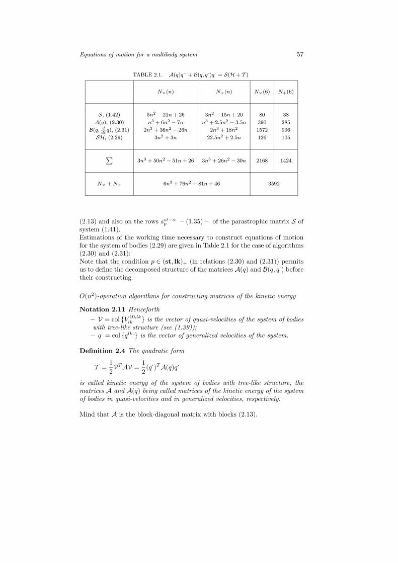
Equations of motion for a multibody system 57
TABLE 2.1. A(q)q·· + B(q, q·)q· = S(H+ T )
N×(n) N+(n) N×(6) N+(6)
S, (1.42) 5n2 − 21n+ 26 3n2 − 15n+ 20 80 38
A(q), (2.30) n3 + 6n2 − 7n n3 + 2.5n2 − 3.5n 390 285
B(q, ddtq), (2.31) 2n3 + 36n2 − 26n 2n3 + 18n2 1572 996
SH, (2.29) 3n2 + 3n 22.5n2 + 2.5n 126 105
P3n3 + 50n2 − 51n+ 26 3n3 + 26n2 − 30n 2168 1424
N× +N+ 6n3 + 76n2 − 81n+ 46 3592
(2.13) and also on the rows sst−αp — (1.35) — of the parastrophic matrix S ofsystem (1.41).Estimations of the working time necessary to construct equations of motionfor the system of bodies (2.29) are given in Table 2.1 for the case of algorithms(2.30) and (2.31):Note that the condition p ∈ (st, lk)+ (in relations (2.30) and (2.31)) permitsus to define the decomposed structure of the matrices A(q) and B(q, q·) beforetheir constructing.
O(n2)-operation algorithms for constructing matrices of the kinetic energy
Notation 2.11 Henceforth
− V = col V 10,lklk is the vector of quasi-velocities of the system of bodieswith tree-like structure (see (1.39));− q· = col qlk. is the vector of generalized velocities of the system.
Definition 2.4 The quadratic form
T = 1
2VTAV = 1
2(q·)TA(q)q·
is called kinetic energy of the system of bodies with tree-like structure, thematrices A and A(q) being called matrices of the kinetic energy of the systemof bodies in quasi-velocities and in generalized velocities, respectively.
Mind that A is the block-diagonal matrix with blocks (2.13).

58 Chapter 2
Proposition 2.16 (Zaremba et al. 1991) There is the following relation
Alk+ = Alklk +
Xst∈(lk)+
LlkstAst+L
lk,Tst (2.32)
where− Alk+ , Ast+ are 6 × 6-dimensional inertia matrices defined for subtrees(lk)+ and (st)+ of the main tree with branches (lk) and (st), respectively;− Llkst ∈ L(R,6) is the matrix of transformation of Est in Elk, (st) ∈(lk)+;− (lk)+ is the set of right incidence of lk-th element of the system (seeDefinition 1.7).
Proof Alk+ =Pst∈(lk)+ L
lkstA
ststL
lk,Tst = LlklkA
lklkL
lk,Tlk +
Pst∈(lk)+ L
lkstA
ststL
lk,Tst =
Alklk +Pst∈(lk)+ L
lkstA
st+L
lk,Tst . 2
Proposition 2.17 Let βlk+ be 6-dimensional row of the kind
βlk+ = Alk+Mlkklk f
lkβ (2.33)
Then− to compute or construct analytically the element Ast−αlk−β from the right-
upper part of the matrix of kinetic energy of the system — O(n2)-operationalgorithm can be used
Ast−αlk−β =½sst−αlk βlk+ if (lk) ∈ (st)+
0 otherwise(2.34)
− for the right-upper part of the matrix of kinetic energy — the matrixrepresentation is fulfilled
A+(q) = SA+MFwhere (recall that S is the parastrophic matrix of system (see (1.42))A+ = diag Alk+, M = diag M lkk
lk , F = diag f lkβ
Proof 1. According to (2.30) we have that
Ast−αlk−β =X
p∈(st,lk)+sst−αp Apps
lk−β,Tp =
Xp∈(st,lk)+
fst,Tα Mstk,Tst Lstp A
ppL
lk,Tp M lkk
lk flkβ =
Xp∈(st,lk)+
fst,Tβ Mstk,Tst LstlkL
lkp A
ppL
lk,Tp M lkk
lk flkβ =
fst,Tβ Mstk,Tst Lstlk(
Xp∈(lk)+
Llkp AppL
lk,Tp )M lkk
lk flkβ =
sst−αlk Alk+Mlkklk f
lkβ = sst−αlk βlk+

Equations of motion for a multibody system 59
2. Equality (2.34) can be proved by multiplication of the matrices from theright-hand side the equality, and using of (2.33). 2
The estimation of the computational working time for algorithm (2.34) (withtaking into account the loss of working time for calculating the matrix S)assumes the following form
N×(n) = 3n2 + 76n− 80, N×(6) = 484 (2.35)
N+(n) = 2.5n2 + 75.5n− 79, N+(6) = 464
Example
The matrix of kinetic energy for double pendulum with sliding hanger is
A(q) =
f1,T2 Θ1+f12 s1−22 Θ2+f
25 s1−23 Θ3+f
36
f2,T5 Θ2+s1−2,T2 f2,T5 Θ2+f
25 s2−53 Θ3+f
36
f3,T6 Θ3+s1−2.T3 f3,T6 Θ3+s
2−5,T3 f3,T6 Θ3+f
36
1− 22− 53− 6
where according to (2.10) and (2.32) Alklk = Θkk, Θ
t+ = Θ
tt + L
tt+1Θ
t+1+ Lt,Tt+1,
Θt+1+ = Θt+1t+1 + Lt+1t+2Θ
t+2+ Lt+1,Tt+2 = Θt+1t+1 as Θ
t+2+ = 0.
O(n)-operation algorithm for constructing b(q, q·)
The straightforward calculation or analytic construction of the column b(q, q·)= B(q, q·)q· in (2.29) can be done by using the O(n3)-operation algorithm(2.31). Belkov (1992) suggested a more effective, linear in n, algorithm forconstructing this column.
Proposition 2.18 Let the algorithm for numerical or analytical constructingof the vector b(q, q·) = B(q, q·)q·, due to (1.41), be taken in the form
b(q, q·) = S(AX + BV), X = ST.q· (2.36)
Then there is a recurrent (from the root of the tree (11) to the branches)O(n)-operation algorithm for constructing the vector X
Xlk = Lµ,k−1,Tlk Xµ,k−1 + Lµ,k−1,T.lk V 10;µ,k−1µ,k−1
X11 = M11k.11 kf11kq11. (2.37)
where the matrices Lµ,k−1,T.lk and M11k.11 are constructed (in numerical or an-
alytical form) by using algorithms (1.22) and (2.19), while vector V 10;µ,k−1µ,k−1 isconstructed by using the kinematical equations for system (1.41) and takinginto account that the matrix S has been constructed at the step of constructingthe matrix A(q).

60 Chapter 2
Proof Producing multiplication for lk-th column Xlk in the right-hand sideof the equality X = ST.q·, we may easily obtain that
Xlk =X
p∈(lk)−sp−α,T.lk qp.α
But it follows from (1.43), that sp−αlk = sp−αµ,k−1Lµ,k−1lk . Hence
Xlk =X
p∈(lk)−(Lµ,k−1,Tlk sp−α,T.µ,k−1 q
p.α + L
µ,k−1,T.lk sp−α,Tµ,k−1 q
p.α ) =
Lµ,k−1,Tlk
Xp∈(lk)−
sp− α,T.µ,k−1 qp.α + L
µ,k−1,T.lk
Xp∈(lk)−
sp−α,Tµ,k−1 qp.α =
Lµ,k−1,Tlk
Xp∈(µ,k−1)−
sp−α,T.µ,k−1 qp.α + L
µ,k−1,T.lk
Xp∈(µ,k−1)−
sp−α,Tµ,k−1 qp.α =
Lµ,k−1,Tlk Xµ,k−1 + Lµ,k−1,T.lk V 10;µ,k−1µ,k−1
as slk−βµ,k−1 = 0. 2
Example
The computation of the vector X for double pendulum with sliding hanger(Fig. 1.4) turns out to be a simple application of the results from Sections1.2.1, 1.3.1, 1.6.2 (see notation (1.23)):
X1 = (M1k1 f
12 )·q1.2 = 0 where M
1k1 f
12 = f
12
X2 = L1,T2 X1 + L1,T.2 V 0,11 = L1,T2 0 + CT.2 (θ
25)f
12 o1.2 =
[w122 ]TCT2 (θ
25)f
12 o1.2 = f
12 o1.2 = 0
X3 = L2,T3 X2 + L2,T.3 V 0,22 = 0 + CT.3 (θ
36)V
0,22 =
[w233 ]TCT3 (θ
36)(s
1−2,T2 o1.2 + s
2−5,T2 θ2.5 ) =
[w233 ]TCT3 (θ36)(0, 1, 0,0)T o1.2 + (0, 0, 1, 0)T θ2.5 =
[w233 ]T (sθ36o
1.2 , cθ
36o1.2 , 0,0)
T + (0, sθ36θ2.5 , cθ
36θ2.5 , 0)
T =
[w233 ]T (sθ36o
1.2 , cθ
36o1.2 , 0, sθ
36θ2.5 , cθ
36θ2.5 , 0)
T =
(cθ36o1.2 θ
3.6 ,−sθ36o1.2 θ3.6 , 0, cθ36θ2.5 θ3.6 ,−sθ36θ2.5 θ3.6 , 0)T
Here [w] = diagw, w for any 3× 3-dimensional matrix w.
Proposition 2.19 Let
− the algorithm for numerical or analytical constructing of the vectorb(q, q·) be presented, with using (1.41), in the form
b(q, q·) = FTMTZ, Z = LY, Y = (AX + BV), X = ST.q·

Equations of motion for a multibody system 61
− the vector X = ST.q· be computed by algorithm (2.37);− (cd) be a bud of the tree.
Then there is the recurrent (from the buds (cd) to the root of the tree (11))O(n)-operation algorithm for constructing the vector Z
Zµ,k−1 = Yµ,k−1 +X
(µ,k−1)+Lµ,k−1lk Zlk, Zcd = Ycd
Proof We shall prove this statement in two steps: in the first, giving arelevant example (Fig. 2.1), we shall explain the idea of the proof, and in thesecond one we shall present the formal proof.The matrix L of the system (see Fig. 2.1) assumes the form
L =
E O ¦ ¦ ¦ ¦ ¦ ¦ ¦O E ¦ ¦ ¦ ¦ O O OO O E O O O O O OO O O E ¦ ¦ O O OO O O O E O O O OO O O O O E O O OO O O O O O E ¦ ¦O O O O O O O E ¦O O O O O O O O E
111213232434424344
41 12 13 23 24 34 42 43 44
where ¦ = Lstlk, (lk) ∈ (st)+, due to the way of defining (1.39).
Figure 2.1. Graph of a multibody system with tree-like structure
After multiplying of the matrix L with the vector Y, we obtain 9 matrixequalities
Z11 = Y11 + L1112Y12 + L
1113Y13 + L
1123Y23 + L
1124Y24 + L
1134Y34 +
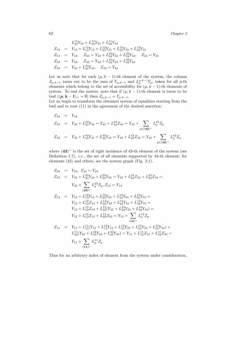
62 Chapter 2
L1142Y42 + L1143Y43 + L
1144Y44
Z12 = Y12 + L1213Y13 + L
1223Y23 + L
1224Y24 + L
1234Y34
Z13 = Y13, Z23 = Y23 + L2324Y24 + L
2334Y34, Z24 = Y24
Z34 = Y34, Z42 = Y42 + L4243Y43 + L
4244Y44
Z43 = Y43 + L4344Y44, Z44 = Y44
Let us note that for each (µ, k − 1)-th element of the system, the columnZµ,k−1 turns out to be the sum of Yµ,k−1 and Lµ,k−1p Yp, taken for all p-thelements which belong to the set of accessibility for (µ, k − 1)-th elements ofsystem. To end the matter, note that if (µ, k − 1)-th element is turns to bebud ((µ,k− 1)+ = ∅) then Zµ,k−1 = Yµ,k−1.Let us begin to transform the obtained system of equalities starting from thebud and to root (11) in the agreement of the desired assertion:
Z44 = Y44
Z43 = Y43 + L4344Y44 = Y43 + L
4344Z44 = Y43 +
Xp∈(43)+
L43p Zp
Z42 = Y42 + L4243Y43 + L
4244Y44 = Y42 + L
4243Z43 = Y42 +
Xp∈(42)+
L42p Zp
where (43)+ is the set of right incidence of 43-th element of the system (seeDefinition 1.7), i.e., the set of all elements supported by 43-th element; forelements (42) and others, see the system graph (Fig. 2.1).
Z34 = Y34, Z24 = Y24
Z23 = Y23 + L2324Y24 + L
2334Y34 = Y23 + L
2324Z24 + L
2334Z34 =
Y23 +X(23)+
L23p Zp, Z13 = Y13
Z12 = Y12 + L1213Y13 + L
1223Y23 + L
1224Y24 + L
1234Y34 =
Y12 + L1213Z13 + L
1223Y23 + L
1224Y24 + L
1234Y34 =
Y12 + L1213Z13 + L
1223(Y23 + L
2324Y24 + L
2334Y34) =
Y12 + L1213Z13 + L
1223Z23 = Y12 +
X(12)+
L12p Zp
Z11 = Y11 + L1112(Y12 + L
1213Y13 + L
1223Y23 + L
1224Y24 + L
1234Y34) +
L1142(Y42 + L4243Y43 + L
4244Y44) = Y11 + L
1112Z12 + L
1142Z42 =
Y11 +X(11)+
L11p Zp
Thus for an arbitrary index of element from the system under consideration,
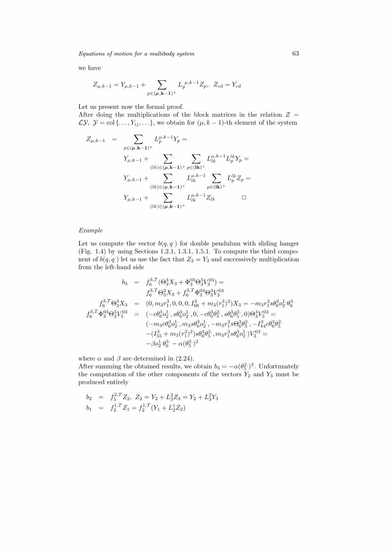
Equations of motion for a multibody system 63
we have
Zµ,k−1 = Yµ,k−1 +X
p∈(µ,k−1)+L µ,k−1p Zp, Zcd = Ycd
Let us present now the formal proof.After doing the multiplications of the block matrices in the relation Z =LY, Y = col . . . , Yij, . . ., we obtain for (µ, k − 1)-th element of the system
Zµ,k−1 =X
p∈(µ,k−1)+Lµ,k−1p Yp =
Yµ,k−1 +X
(lk)∈(µ,k−1)+
Xp∈(lk)+
Lµ,k−1lk Llkp Yp =
Yµ,k−1 +X
(lk)∈(µ,k−1)+Lµ,k−1lk
Xp∈(lk)+
Llkp Zp =
Yµ,k−1 +X
(lk)∈(µ,k−1)+Lµ,k−1lk Zlk 2
Example
Let us compute the vector b(q, q·) for double pendulum with sliding hanger(Fig. 1.4) by using Sections 1.2.1, 1.3.1, 1.5.1. To compute the third compo-nent of b(q, q·) let us use the fact that Z3 = Y3 and successively multiplicationfrom the left-hand side
b3 = f3,T6 (Θ33X3 +Φ033 Θ
33V
033 ) =
f3,T6 Θ33X3 + f3,T6 Φ033 Θ
33V
033
f3,T6 Θ33X3 = (0,m3r31, 0, 0, 0, I
366 +m3(r
31)2)X3 = −m3r
31sθ
36o1.2 θ
3.6
f3,T6 Φ033 Θ33V
033 = (−cθ36o1.2 , sθ36o1.2 , 0,−cθ36θ2.5 , sθ36θ2.5 , 0)Θ33V 033 =
(−m3cθ36o1.2 ,m3sθ
36o1.2 ,−m3r
31sΘ
36θ2.5 ,−I344cθ36θ2.5
−(I355 +m3(r31)2)sθ36θ
2.5 ,m3r
31sθ
36o1.2 )V
033 =
−βo1.2 θ3.6 − α(θ2.5 )2
where α and β are determined in (2.24).After summing the obtained results, we obtain b3 = −α(θ2.5 )2. Unfortunatelythe computation of the other components of the vectors Y2 and Y3 must beproduced entirely
b2 = f2,T5 Z2, Z2 = Y2 + L23Z3 = Y2 + L
23Y3
b1 = f1,T2 Z1 = f1,T2 (Y1 + L
12Z2)
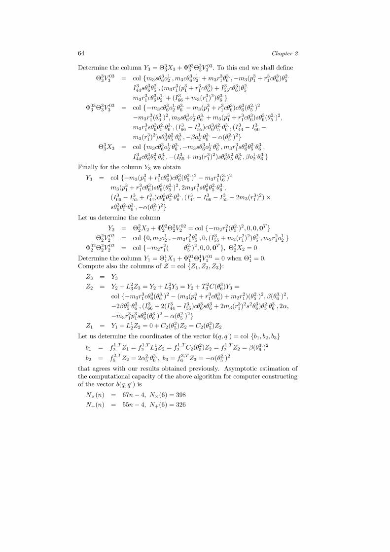
64 Chapter 2
Determine the column Y3 = Θ33X3 +Φ
033 Θ
33V
033 . To this end we shall define
Θ33V033 = col m3sθ
36o1.2 ,m3cθ
36o1.2 +m3r
31θ3.6 ,−m3(p
31 + r
31cθ
36)θ
2.5
I344sθ36θ2.5 , (m3r
31(p
31 + r
31cθ
36) + I
355cθ
36)θ
2.5
m3r31cθ
36o1.2 + (I
366 +m3(r
31)2)θ3.6
Φ033 Θ33V
033 = col −m3cθ
36o1.2 θ
3.6 −m3(p
31 + r
31cθ
36)cθ
36(θ
2.5 )
2
−m3r31(θ
3.6 )
2,m3sθ36o1.2 θ
3.6 +m3(p
31 + r
31cθ
36)sθ
36(θ
2.5 )
2,
m3r31sθ
36θ2.5 θ
3.6 , (I
366 − I355)cθ36θ2.5 θ3.6 , (I344 − I366 −
m3(r31)2)sθ36θ
2.5 θ
3.6 ,−βo1.2 θ3.6 − α(θ2.5 )
2Θ33X3 = col m3cθ
36o1.2 θ
3.6 ,−m3sθ
36o1.2 θ
3.6 ,m3r
31sθ
36θ2.5 θ
3.6 ,
I344cθ36θ2.5 θ
3.6 ,−(I355 +m3(r
31)2)sθ36θ
2.5 θ
3.6 ,βo
1.2 θ
3.6
Finally for the column Y3 we obtain
Y3 = col −m3(p31 + r
31cθ
36)cθ
36(θ
2.5 )
2 −m3r31(3.6 )
2
m3(p31 + r
31cθ
36)sθ
36(θ
2.5 )
2, 2m3r31sθ
36θ2.5 θ
3.6 ,
(I366 − I355 + I344)cθ36θ2.5 θ3.6 , (I344 − I366 − I355 − 2m3(r31)2)×
sθ36θ2.5 θ
3.6 ,−α(θ2.5 )2
Let us determine the column
Y2 = Θ22X2 +Φ022 Θ
22V
022 = col −m2r
21(θ
2.5 )
2, 0, 0,0TΘ22V
022 = col 0,m2o
1.2 ,−m2r
21θ2.5 , 0, (I
355 +m2(r
21)2)θ2.5 ,m2r
21o1.2
Φ022 Θ22V
022 = col −m2r
21( θ2.5 )
2, 0, 0,0T , Θ22X2 = 0Determine the column Y1 = Θ
11X1 +Φ
011 Θ
11V
011 = 0 when Θ11 = 0.
Compute also the columns of Z = col Z1, Z2, Z3:Z3 = Y3
Z2 = Y2 + L23Z3 = Y2 + L
23Y3 = Y2 + T
23C(θ
36)Y3 =
col −m3r31cθ
36(θ
3.6 )
2 − (m3(p31 + r
31cθ
36) +m2r
21)(θ
2.5 )
2,β(θ3.6 )2,
−2βθ2.5 θ3.6 , (I366 + 2(I344 − I355)cθ36sθ36 + 2m3(r31)2s2θ36)θ
2.5 θ
3.6 , 2α,
−m3r31p31sθ
36(θ
3.6 )
2 − α(θ2.5 )2
Z1 = Y1 + L12Z2 = 0 + C2(θ
25)Z2 = C2(θ
25)Z2
Let us determine the coordinates of the vector b(q, q·) = col b1, b2, b3b1 = f1,T2 Z1 = f
1,T2 L12Z2 = f
1,T2 C2(θ
25)Z2 = f
1,T2 Z2 = β(θ3.6 )
2
b2 = f2,T5 Z2 = 2α2.5 θ
3.6 , b3 = f
3,T6 Z3 = −α(θ2.5 )2
that agrees with our results obtained previously. Asymptotic estimation ofthe computational capacity of the above algorithm for computer constructingof the vector b(q, q·) is
N×(n) = 67n− 4, N×(6) = 398N+(n) = 55n− 4, N+(6) = 326

Equations of motion for a multibody system 65
TABLE 2.2. A(q)q·· + b(q, q·) = SH
N×(n) N+(n) N×(6) N+(6)
S, (1.42) 5n2 − 21n+ 26 3n2 − 15n+ 20 80 38
A(q), (2.30) n3 + 6n2 − 7n n3 + 2.5n2 − 3.5n 390 285
b(q, ddtq), (2.31) 67n2 − 4n 55n− 4 398 326
SH, (2.29) 3n2 + 3n 22.5n2 + 2.5n 126 105
Pn3 + 14n2 + 42n+ 22 n3 + 8n2 + 39n+ 16 994 754
N× +N+ 2n3 + 22n2 + 81n+ 38 1748
Figure 2.2. Graphic illustration of computational wastes
N(n) = N× +N+ from tables 2.2 and 2.3
Estimation of computational complexity of the computer-aided algorithms
Estimations of computational complexity of the algorithms are given in tables2.2-2.7. Table 2.2 presents estimations of the computational complexity of analgorithm for constructing the equations of motion, which realized on the basisof use of O(n3)-operation algorithm (2.30) for constructing the matrix A(q)
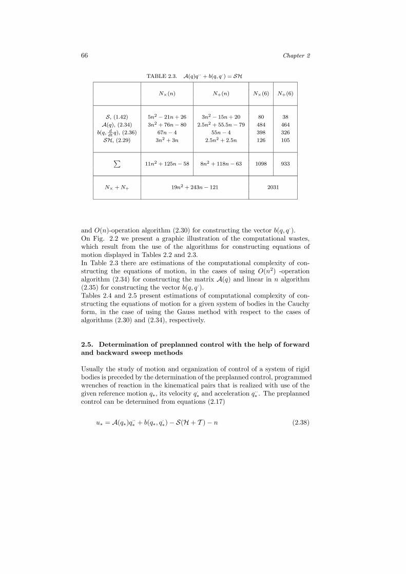
66 Chapter 2
TABLE 2.3. A(q)q·· + b(q, q·) = SH
N×(n) N+(n) N×(6) N+(6)
S, (1.42) 5n2 − 21n+ 26 3n2 − 15n+ 20 80 38
A(q), (2.34) 3n2 + 76n− 80 2.5n2 + 55.5n− 79 484 464
b(q, ddtq), (2.36) 67n− 4 55n− 4 398 326
SH, (2.29) 3n2 + 3n 2.5n2 + 2.5n 126 105
P11n2 + 125n− 58 8n2 + 118n− 63 1098 933
N× +N+ 19n2 + 243n− 121 2031
and O(n)-operation algorithm (2.30) for constructing the vector b(q, q·).On Fig. 2.2 we present a graphic illustration of the computational wastes,which result from the use of the algorithms for constructing equations ofmotion displayed in Tables 2.2 and 2.3.In Table 2.3 there are estimations of the computational complexity of con-structing the equations of motion, in the cases of using O(n2) -operationalgorithm (2.34) for constructing the matrix A(q) and linear in n algorithm(2.35) for constructing the vector b(q, q·).Tables 2.4 and 2.5 present estimations of computational complexity of con-structing the equations of motion for a given system of bodies in the Cauchyform, in the case of using the Gauss method with respect to the cases ofalgorithms (2.30) and (2.34), respectively.
2.5. Determination of preplanned control with the help of forwardand backward sweep methods
Usually the study of motion and organization of control of a system of rigidbodies is preceded by the determination of the preplanned control, programmedwrenches of reaction in the kinematical pairs that is realized with use of thegiven reference motion q∗, its velocity q·∗ and acceleration q··∗ . The preplannedcontrol can be determined from equations (2.17)
u∗ = A(q∗)q··∗ + b(q∗, q·∗)− S(H+ T )− n (2.38)

Equations of motion for a multibody system 67
TABLE 2.4. q·· = A−1(q)(SH− b(q, q·)) (Gauss method)
N×(n) N+(n) N×(6) N+(6)
Pn3 + 14n2 + 42n+ 22 n3 + 8n2 + 39n+ 16 994 754
Gauss 13n3 + 3
2n2 + 1
6n 1
3n3 + 3
2n2 + 1
6n 127 127
PP43n3 + 31
2n2 + 253
6n+ 22 4
3n3 + 19
2n2 + 235
6n+ 16 1121 881
N× +N+ 83n3 + 25n2 + 81.33n+ 38 2002
TABLE 2.5. q·· = A−1(q)(SH− b(q, q·)) (Gauss method)
N×(n) N+(n) N×(6) N+(6)
P11n2 + 125n− 58 8n2 + 118n− 63 1098 993
Gauss 13n3 + 3
2n2 + 1
6n 1
3n3 + 3
2n2 + 1
6n 127 127
PP13n3 + 25
2n2 + 751
6n− 58 1
3n3 + 19
2n2 + 709
6n− 63 1215 1060
N× +N+ 23n3 + 22n2 + 243.33n− 121 2275
but to this end, a preliminary construction of all vector and matrices whichcomposed (2.38) must be done. Hence there will be preliminary calculationexpenditures as these shown in Tables 2.2 and 2.3. Let us remark also thatpreplanned wrenches of reaction in the kinematical pairs are not defined by(2.38).In this section, we present the results from development of effective (in thecomputational respect) algorithms for determination of the all necessary pre-planned forces without using equations of motion in the (2.38)-form. Thereare two such algorithms (Juravlev et al. 1993):

68 Chapter 2
− the first algorithm is based on the so called forward sweep method for cal-culating preplanned quasi-velocities and quasi-accelerations of the bodiesfrom the system;
− the second one is based on the backward sweep method for calculatingpreplanned control and wrenches of reaction in kinematical pairs.
Let us now expound the algorithm based on the forward sweep on the back-ward sweep method of computing the preplanned quasi-velocities and quasi-accelerations of the bodies from the system.
Proposition 2.20 Let
− the main kinematical equality of the system of bodies have the (1.28)-kind form, where again (1.31) is taken into account;− qlk∗ , qlk.∗ , qlk..∗ be given reference motions, velocities, and accelerations forthe kinematical pairs of the system.
Then
− the recurrent algorithm of forward sweep method of computing pre-planned quasi-velocities of bodies of the system has following form
V 10,lklk∗ = Lµ,k−1,Tlk∗ V 10;µ,k−1µ,k−1∗ +M lkklk∗ kf lkkqlk.∗ (2.39)
V 10,1111∗ = M11k11∗ kf11kq11.∗
− the recurrent algorithm of the forward sweep method for computing pre-planned quasi-accelerations of the system of bodies has the following form
V 10,lk.lk∗ = Φµ,k−1;lk,Tlk∗ Lµ,k−1,Tlk∗ V 10;µ,k−1µ,k−1∗ + Lµ,k−1,Tlk∗ V 10;µ,k−1.µ,k−1∗ +
M lkk.lk∗ kf lkkqlk.∗ +M lkk
lk∗ kf lkkqlk..∗ (2.40)
V 10,1.11∗ = M11k11∗ kf11kq11..∗ +M11k.
11∗ kf11kq11.∗
To prove this statement is enough to written down equality (1.28) in recurrentform and differentiate it taking in account equality (1.22).Let us carry out an estimation of the computational capacity of algorithms(2.39) and (2.40) for kinematical chains with rotating kinematic pairs of fifthorder, in the case of constructive parallel translation along one of the coordi-nates.
N×(n) = 38n, N×(6) = 228, N+(n) = 24n, N+(6) = 144 (2.41)
Let us now expound the algorithm based on the backward sweep methodof computing control and wrenches of reactions in kinematical pairs of thesystem.
Proposition 2.21 Let
− there be no interactions between elements of the system of bodies withthe bodies of the external medium;

Equations of motion for a multibody system 69
− equations of motion for each body of the system have the (2.13)-kindform
AlklkV10,lk.lk +BlklkV
10,lklk = Zlklk +H
lklk + T
lklk
Zlklk = Zlklk (µ, k − 1; lk)−
Xi
Llki,k+1Zi,k+1i,k+1(lk; i, k + 1)
where the (2.9)-kind form is used for forming Z with corresponding in-dices;− Ri,k+1i,k+1(lk; i, k + 1) = 0 if lk-th body turns out to be a leaf (last body ofsome branch) (this can be considered as a corollary from the first pro-posal).
Then the recurrent algorithm for computing preplanned wrenches of reactionsand control forces in kinematical pairs can be written as
Rlklk∗(µ, k − 1; lk) +N lklk∗(µ, k − 1; lk) + U lklk∗(µ, k − 1; lk) =
AlklkV10,lk.lk∗ +Blklk∗V
10,lklk∗ +
Xi
Llki,k+1∗(Ri,k+1i,k+1∗(lk; i, k + 1) +
N i,k+1i,k+1∗(lk; i, k + 1) + U
i,k+1i,k+1∗(lk; i, k + 1))−H lk
lk∗ − T lklk∗ (2.42)
with using the fact that non-trivial coordinates from the wrenches N lklk∗(µ, k−
1; lk)+U lklk∗(µ, k− 1; lk) stand at the positions of the zeros in wrenches of thereaction Rlklk∗(µ, k − 1; lk) and vice versa.
The estimation of computational expenditures of algorithm (2.42) is linear inn
N×(n) = 26n, N×(6) = 156, N+(n) = 20n, N+(6) = 120 (2.43)
After summation of (2.41) and (2.43) we obtain the total estimation for theforward and backwad sweep methods
N×(n) = 64n, N×(6) = 384, N+(n) = 44n, N+(6) = 264
2.6. Algorithm for constructing equations of motion based on for-ward and backward sweep methods
In this final section we shall demonstrate another algorithm for constructingthe equations of motion for a system of rigid bodies. Although it is moreeffective that the other ones, unfortunately it is valid only for the case ofno mechanical contact of bodies of the system with bodies from the externalmedium. This is due to the fact that it is based on using forward and backwardsweep methods, the latter being valid only under the above condition.

70 Chapter 2
Proposition 2.22 Let
− bodies from the system have no mechanical contact with bodies from theexternal medium;− Ro(µ, k− 1; lk), Uo(µ, k− 1; lk), No(µ, k− 1; lk) be the columns of thewrenches of action of (µ, k−1)-th body to lk-th body determined for q·· =0 (q·· is the generalized acceleration of the system), with correspondingmeaning indicated by Ro, Uo and No (reaction, control and friction);− the algorithm of forward sweep method for determination of quasi-veloci-ties and quasi-accelerations in the case of q·· = 0 be presented as
V 10,lklko = Lµ,k−1,Tlko V 10;µ,k−1µ,k−1o +M lkklko kf lkkqlk.o
V 10,lk.lko = Φµ,k−1;lk,Tlko Lµ,k−1,Tlko V 10;µ,k−1µ,k−1o +
Lµ,k−1,Tlko V 10;µ,k−1.µ,k−1o +M lkk.lko kf lkkqlk.o
V 10,11.11o = M11k.11o kf11kq11.o
− for calculating the wrenches Rlklko(µ, k−1; lk), U lklko(µ, k−1; lk), N lklko(µ,
k − 1; lk) there be the following algorithm of backward sweep method
Rlklko(µ, k − 1; lk) +N lklko(µ, k − 1; lk) + U lklko(µ, k − 1; lk) =
AlklkoV10,lk.lko +BlklkV
10,lklko +
Xi
Llki,k+1o(Ri,k+1i,k+1o(lk; i, k + 1) +
N i,k+1i,k+1o(lk; i, k + 1) + U
i,k+1i,k+1o(lk; i, k + 1))−H lk
lk∗ − T lklk∗ (2.44)Then the equations of motion for the system of bodies having no relation withbodies from the external medium can be presented as
A(q)q·· + d(q, q·) = u+ n (2.45)
where the vector d(q, q·) is determined by the relation
d(q, q·) = FTMTZo(µ, k − 1; lk) (2.46)
Z(µ, k − 1; lk) = Ro(µ, k − 1; lk) + Uo(µ, k − 1; lk) +No(µ, k − 1; lk)
Proof Multiplying system (2.13), written down in the matrix form, fromthe left-hand side withMTL (it comes from the right-hand side of the matrixS = FTMTZ) and using (1.41) we obtain
MTLALTMFq·· + MTLb(q, q·) =MTL(H+ T ) +MTL(R+ U +N ) (2.47)
Moreover, zeros in the reaction columnsMTLU and the friction onesMTLNcorrespond to the non-zero coordinates of the control columnsMTLR whichpresent reactions in the kinematical pairs, and vice versa. It is the relationthat is used to eliminate reactions in the kinematical pairs and to separatecontrol and friction forces, by means of multiplication from the left with thematrix FT of the mobility axes.

Equations of motion for a multibody system 71
Formally we may determine such forces Ro of reaction, Uo of control and Noof friction for the kinematical pairs that the generalized acceleration q·· of thesystem will be zero. For these forces we obtain, due to (2.47), that the columnFo must satisfy
MTLb(q, q·) =MTL(H+ T ) + Fo (2.48)
where
Fo = MTL(Ro+Uo+N o) =MT [Ro(µ, k − 1; lk) +Uo(µ, k − 1; lk) +No(µ, k − 1; lk)]
Calculation of Ro(µ, k − 1; lk), Uo(µ, k − 1; lk) and No(µ, k − 1; lk) is doingby the algorithms of forward and backward sweep methods for q·· = 0 (see(2.44)).Subtracting equality (2.48) from (2.47), we obtain the following equality
MTLALTMF q·· =MTL(R+ U +N )− Fo
Multiplying this equality from the left with FT , we cut out from this systemthe equations for which FTMTLR = 0 and also these for which u+ n =FTMTL(U +N ). This completes the proof.2
Example: Double pendulum with sliding hanger (Fig. 1.4)
Due to the notations adopted in (2.45) and the above results concerning thispart of the system
d(q, q·) =
d1d2d3
=
f1,T2 0 0
0 f2,T5 0
0 0 f3,T6
Z11(0, 1)Z22(1, 2)Z33(2, 3)
Θ11 ≡ 0 (2.49)
V 011 = (0, o1.2 , 0,0)T , V 022 = (0, o1.2 , 0, 0, θ
25 ,0)
T
V 033 = (o1.2 sθ36, o
1.2 cθ
36,−p31θ2.5 , sθ36θ2.5 , cθ36θ2.5 , θ3.6 )T
V 01.1 = V 02.2 = 0 for q·· = 0V 03.3 = (cθ36o
1.2 θ
3.6 ,−sθ36o1.2 θ3.6 , 0, cθ36θ2.5 θ3.6 ,−sθ36θ2.5 θ3.6 , 0)T
According to (2.44) we obtain
Z33(2, 3) = Θ33V03.3 +Φ033 Θ
33V
033 − F 33 , F 33 = H3
3 + T33
Z22(1, 2) = Θ22V02.2 +Φ022 Θ
22V
022 + L23Z
33(2, 3)− F 22
F 22 = H22 + T
22
Z11(0, 1) = L12Z22(1, 2)− F 11 , F 11 = P 11 + T 11 , V 01.1 = 0

72 Chapter 2
Calculating
d3 = −α(θ2.5 )2 − f3,T6 F 33 (2.50)
we have
d3 = f3,T6 Z33(2, 3) = (0,0, 0, 1)Θ33V
03.3 + (0,0, 0, 1)Φ033 Θ
33V
033
−f3,T6 F 33 = (0,m3r31,0,(I
366 +m3(r
31)2))V 03.3 +
(−cθ36o1.2 , sθ36o1.2 , 0,−cθ36θ2.5 , sθ36θ2.5 , 0)Θ33V 033 − f3,T6 F 33 =
−m3r31sθ
36o1.2 θ
3.6 + (−m3cθ
36o1.2 ,m3sθ
36o1.2 ,−m3r
31sθ
36θ2.5 ,
I344cθ36θ2.5 , (I
355 +m3(r
31)2)sθ36θ
2.5 ,m3r
31sθ
36o1.2 )V
033 −
f3,T6 F 33 = −α(θ2.5 )2 − f3,T6 F 33
Computing now
d2 = 2αθ2.5 θ
3.6 − f
2,T5 F 22 − f
2,T5 L23F
33
we get
d2 = f2,T5 Z22(1, 2) = f2,T5 θ22V
02.2 + f2,T5 Φ022 Θ
22V
022 +
f2,TL23Z33(2, 3)− f
2,T5 F 22 = f
2,T5 L23Z
33 (2, 3)− f
2,T5 F 22 =
f2,T5 T 223 C23 (Θ
33V
03.3 +Φ033 Θ
33V
033 )− f
2,T5 (L23F
33 − F 22 ) =
f2,T5 T 223 C23Θ
33V
03.3 + f2,T5 T 223 C
23Φ
033 Θ
33V
033 − f
2,T5 L23F
33 =
α2.5 θ3.6 + α2.5 θ
3.6 − f
2,T5 F 22 − f
2,T5 L23F
33
Let us now determine
d1 = β(θ3.6 )2 − f1,T2 F 11 − f
1,T2 L12F
22 − f
1,T2 L12L
23F
33 (2.51)
then
d1 = f1,T2 Z11(0, 1) = f1,T2 L12Z
22(1, 2)− f
1,T2 F 11 =
f1,T2 L12(Θ22V
02.2 +Φ022 Θ
22V
022 + L23Z
33(2, 3)− F 22 )− f
1,T5 F 11 =
f1,T2 L12Θ22V
02.2 + f1,T2 L12Φ
022 Θ
22V
022 + f1,T2 L12L
23Z
33(2, 3)
−f1,T2 L12F22 − f
1,T5 F 11 = f
1,T2 L12Φ
022 θ22V
022 +
f1,T2 L13(Θ33V
03.3 +Φ033 Θ
33V
033 )− f
1,T2 L13F
33 − f
1,T2 L12F
22 −
f1,T5 F 11 = 0 + 0 + f1,T2 L13Φ
033 Θ
33V
033 − f
1,T2 L13F
33 − f
1,T2 L12F
22 −
f1,T5 F 11 = −m3r31sθ
36(θ
3.6 )
2 − f1,T2 L13F33 − f
1,T2 L12F
22 − f
1,T2 F 11 =
β(θ3.6 )2 − f1,T2 L13F
33 − f
1,T2 L12F
22 − f
1,T2 F 11

Equations of motion for a multibody system 73
TABLE 2.6. A(q)q·· + d(q, q·) = u+ n
N×(n) N+(n) N×(6) N+(6)
S, (1.42) 5n2 − 21n+ 226 3n2 − 15n+ 20 80 38
A(q), (2.30) n3 + 6n2 − 7n n3 + 2.5n2 − 3.5n 390 285
d(q, ddtq), (2.46) 64n 44n 384 264
Pn3 + 11n2 + 36n+ 26 n3 + 5.5n2 + 25.5n+ 20 854 587
N× +N+ 2n3 + 16.5n2 + 61.5n+ 46 1441
TABLE 2.7. A(q)q·· + d(q, q·) = u+ n
N×(n) N+(n) N×(6) N+(6)
S, (1.42) 5n2 − 21n+ 226 3n2 − 15n+ 20 80 38
A(q), (2.34) 3n2 + 76n− 80 2.5n2 + 55.5n− 79 484 464
d(q, ddtq), (2.46) 64n 44n 384 264
P8n2 + 119n− 54 5.5n2 + 104.5n− 59 948 766
N× +N+ 13.5n2 + 223.5n− 113 1714
After summing equalities (2.50)-(2.51), we obtain
d(q, q·) =
d1d2d3
=
β(θ3.6 )2
2αθ2.5 θ3.6
−α(θ2.5 )2
− S(H+ T ) =
b(q, q·)− S(H+ T ) (2.52)

74 Chapter 2
Substituting with (2.52) in equation (2.49), we have the equations of motionin the following form
A(q)q·· + b(q, q·) = S(H+ T ) + u+ n
This form of the equations was obtained previously in another way (see (2.17)).In Tables 2.6 and 2.7 there is the estimation of computational expenditureswhich are due to using algorithm (2.52) for constructing the matrix A(q)together with one of algorithms (2.30) or (2.34).Fig. 2.3 presents diagrammatic comparison of the computational complexityof the algorithms from Tables 2.6 and 2.7.
Figure 2.3. Graphic illustration of computational wastes
N(n) = N× +N+ from tables 2.6 and 2.7

Chapter 3
Analytic transvective forms of dynamic equationsin the Cauchy form
This chapter defines factorization of inertia matrix and its inverse for a multi-body system with tree-like structure through the simplest multipliers - trans-vections that gives possibility to analytical studying and numerical solvingthe Cauchy problem for a multibody system having a rather large dimensionwith the help of computer algebra methods (Gerdt et al. 1980, Grosheva etal. 1983, Klimov et al. 1989) and standard algebraic software. In particular,the inverse resolution is obtained without constructing the inertia matrix it-self. It is essential that the properties of aggregative form of representation ofmultibody system equations are used here (Konoplev 1989a and 1990). Formultibody systems, the transvective Cauchy form is considered, computer la-boriousness of the algorithms obtained being estimated (Konoplev 1992 and1995). For constructing entries At−αk−β of the inertia matrix A(q) of the multi-body system (2.30), (2.34) two algorithms are obtained in Chapter 2. Thefirst one is
At−αk−β =X
p∈(t,k)+st−αp Apps
k−β,Tp , st−αk = f t,Tα Ltk (3.1)
The second one is
At−αk−β = st−αk βk+, k ∈ (t)+, At−αk−β = 0, k /∈ (t)+ (3.2)
βk+ = Ak+fkβ , A
k+ = A
kk +
Xp∈(k)+
LkpAp+L
k,Tp (3.3)
where
α = α(t), β = β(k) (α,β = 1, 6)
75

76 Chapter 3
3.1. Matrix realization of Gauss method
Notation 3.1 Henceforth
− GL(R,n) is the full linear group of automorphisms of Rn (i.e., thegroup of invertible n× n-dimensional matrices A, det A 6= 0) (Bourbaki1969, Diedonne 1972, Suprunenko 1972);− SL(R,n) ⊂ GL(R,n) is the special linear group of automorphisms ofRn (the group of invertible n× n-dimensional matrices A, det A = 1);− Eij is n×n-dimensional matrix with a unit at the place (i, j) and zerosat all other ones;− E is n× n identity matrix.
Any a ∈ R1, define matrices
tij(a) = E + aEij ∈ SL(R,n), t−1ij (a) = tij(−a) (3.4)
known as transvections (Gantmacher 1964, Suprunenko 1972).
Proposition 3.1 The next assertions hold:
− transvections constitute the set of generatrices of the group SL(R,n);− the set of transvections and the set of diagonal ones tj(b), b ∈ R1, b 6=0, of the kind
tj(b) = E + (b− 1)Ejj (3.5)
t−1j (b) = tj(1/b),Qtj(bj) = diag bj (3.6)
constitute the set of generatrices of the group GL(R,n) (Gantmacher
1964, Suprunenko 1972);− multiplying any A ∈ GL(R,n) on the transvection tij(a) from the left-hand side leads to multiplying j-row of the matrix A on the number a andadding with i-row;− multiplying any A ∈ GL(R,n) on the transvection tij(a) from the right-hand side leads to multiplying i-column of the matrix A on the number aand adding with j-column;− multiplying any A ∈ GL(R,n) on the matrix tj(b) from the left-handside leads to multiplying j-row of the matrix A on the number b.
It follows from the above proposition that the generatrices tij(a) and tj(b)realize elementary transformations of Gauss method and therefore this methoditself with the help of corresponding choice of the numbers a and b.
3.2. Analytic transvective forms of inertia matrix and its inverse
Due to (3.1)—(3.3), the attractive feature of aggregative form of inertia matrixrepresentation is that in the Gauss method arguments of matrices (3.4) and

Analytic transvective forms of dynamic equations in the Cauchy form 77
(3.5) with arbitrary indexes are represented by inner products of the (3.2)-kind, the first multiplier not depending on the method pre-history (it is thesame as in (3.2)) while the second one is defined by a recurrence algorithm ofsymbolical constructing or computing and takes account this pre-history.
Notation 3.2 Henceforth
− Ak∆k is 6× 6-dimensional matrix of the following kindAk∆k = Akk +∆
kk
where the matrix ∆kk is defined by the recurrence relation
∆kk =X
p∈(k)+Lkp(A
p∆p − βp∆p βp∆,Tp (β,β)p∆p )Lk,Tp (3.7)
− βk∆k is β-column of the matrix Ak∆k (β = 1, 6)
βk∆k = Ak∆k fkβ
− (β,β)k∆k is (β,β)-entry of the matrix Ak∆k
(β,β)k∆k = fk,Tβ βk∆k = fk,Tβ Ak∆k fkβ
− βk∆k is the column defined by the following relation
βk∆k = βk∆k /(β,β)k∆k
− ht, ki is the inner product (being similar to (3.2)) of the kindht, ki = st−αk βk∆k (3.8)
− ttk(ht, ki), t < k, is transvection (3.4) with the argument ht, ki;− T is product of transvections zeroing above-diagonal entries of the ma-trix A(q) in the Gauss method starting from the last row
T =Qt,k
t−1tk (ht, ki), t < k (3.9)
T T =Qt,k
t−1tk (ht, ki)T =Qt,k
t−1kt (hk, ti), t < k
ttk(ht, ki)T = tkt(hk, ti) (3.10)
Proposition 3.2 The following equality holds
T A(q)T T = diag (β,β)k∆k =Qk
tk(β,β)k∆k (3.11)
For example, for two link mechanism with kinematical pairs of the fifth classit follows from (3.1) and the relation A2∆2 = A22 that
A(q) ="f1,Tβ A11f
1β + s
1−α2 A2∆2 f2β s1−β2 β2∆2
s1−β2 β2∆,T2 (β,β)2∆2
#

78 Chapter 3
Multiplying the last relation from the left-hand side on
t−112 (s1−β2 β2∆2 /(β,β)2∆2 ) = t−112 (s
1−β2 β2∆2 )
we get zero at the place (1, 2) and the relation
A1−β1−β = f1,Tβ A11f1β + s
1−β2 A2∆2 f2β − s
1−β2 β2∆2 (s1−β2 β2∆2 )T (β,β)2∆2 =
f1,Tβ A11 + L12A2∆2 − β2∆2 β2∆,T2 (β,β)2∆2 L1,T2 f1,Tβ =
f1,Tβ (A11 +∆11)f
1β = f
1,Tβ β1∆1 = (β,β)1∆1
at the place (1, 1). Multiplying the matrix t−112 (s1−β2 β2∆2 )A(q) from the right-
hand side on the transvection t−121 (s1−β2 β2∆2 ) we have the desired result (3.11)
T A(q)T T = t−112 A(q)t−121 = diag t1(β,β)1∆1 , t2(β,β)2∆2
Notation 3.3 Henceforth
− βkδ+ is (similarly to (3.3)) β -column of some 6× 6-dimensional matrixAkδ+ not being used directly;− (β,β)kδ+ is (β,β)-entry of the matrix Akδ+
(β,β)kδ+ = fk,Tβ βkδ+ (3.12)
− βkδ+ is the column defined by the relation
βkδ+ = βkδ+ /(β,β)kδ+ (3.13)
Proposition 3.3 Let the recurrence algorithm of numerical or symbolicalconstructing of the column βkδ+ take the form (for βk+ from (3.3))
βkδ+ = βk+ − δk+ (3.14)
δk+ =X
p∈(k)+\(k)L(k, p)LT (k, p)fkβ (β,β)
pδ+ (3.15)
L(k, p) = Lkpβpδ+ = Lkk+1L(k + 1, p), L(p, p) = βpδ+
Then (similarly to (3.11)) there holds the following equality
T A(q)T T = diag (β,β)kδ+ =Qk
tk(β,β)kδ+ (3.16)
where ht, ki is the inner product of the kind
ht, ki = st−αk βkδ+ , st−αk = f t,Tα Ltk (3.17)

Analytic transvective forms of dynamic equations in the Cauchy form 79
For example, for two link mechanism we have
A(q) ="
f1,Tβ β1+ s1−β2 β2δ+β2δ,T+ s1−β,T2 (β,β)2δ+
#, β2δ+ = β2+
With multiplying the matrix on the transvection t−112 (s1−β2 β2δ+ ) from the left-
hand side, the above left entry assumes the form
A1−β1−β = f1,Tβ β1+ − s1−β2 β2δ+ β2δ,T+ s1−β,T2 /(β,β)2δ+ =
f1,Tβ β1+ − f1,Tβ L12β
2δ+ β2δ,T+ s1−β,T2 (β,β)2δ+ (β,β)2δ+ −2 =
f1,Tβ β1+ − L12β2δ+ (L12β2δ+ )T f1β(β,β)2δ+ =f1,Tβ β1+ − L(1, 2)LT (1, 2)f1β(β,β)2δ+ =f1,Tβ β1+ − δ1+ = f1,Tα β1δ+ = (β,β)1δ+
It follows from the multiplying of the obtained matrix on t−121 (s1−β2 β2δ+ ) from
the right-hand side that equality (3.16) holds.For three link mechanism and a tree-like system with n = 5 independentlyfrom the algorithm of constructing transvection arguments, we have (respec-tively)
T = t−112 t−113 t−123 , T = t−111,12 t−111,13 t−112,13 t−111,23 t−112,23 t−111,32Therefore due to (3.11) and (3.16), we have the following main results, namely:algorithms of straight analytical or numerical constructing matrices A(q) andA−1(q).
Proposition 3.4 Due to (β,β)kζ = (β,β)kδk = (β,β)kδ+ , there are the analyt-ical transvective forms of matrices A(q) and A−1(q)
A(q) = T −1diag (β,β)kζk (T −1)T (3.18)
A−1(q) = T Tdiag 1/(β,β)kζk T (3.19)
Proving these assertions follows from (3.11) and (3.16) with according to (3.9)—(3.10).Note that together with constructing transvective expansion of the inverseA−1(q), with the help of algorithm (3.8), here the matrix A(q) is formed asalgorithm (3.2) is the first term of algorithm (3.8) multiplied on (β,β)kδ+ .
3.3. Analytical transvective Cauchy form of motion equations fora tree-like system
One of main applications of the results obtained is the possibility of straightuse of analytical (with the help of computer algebra methods (Aleksandrov

80 Chapter 3
TABLE 3.1. q·· = A−1(q)(SH− b(q, q·))
N×(n) N+(n) N×(6) N+(6)
S, (1.42) 5n2 − 21n+ 26 3n2 − 15n+ 20 80 38
A(q), (3.8) 375n− 369 327n− 306 1881 1656
b(q, q), (2.36) 67n− 4 55n− 4 398 326
SH, (2.29) 3n2 + 3n 2.5n2 + 2.5n 126 105
SH − b(q, q) = F 6 0 6
q = A(q)F 2n2 n2 − n 72 30
P10n2 + 424n− 347 6.5n2 + 386.5n− 284 2557 2161
N× +N+ 16.5n2 + 810.5n− 631 4718
1980, Arais et al. 1987, Bahman 1969) or numerical (with the help of standardsoftware) constructing equations (2.17) in the Cauchy form: q·· = F - withoutdefining the matrix A(q) and its inverse.
Proposition 3.5 The analytical transvective Cauchy form of motion equa-tions for a multibody system with tree-like structure is
q·· = T Tdiag 1/(β,β)kζT F , F = Q− b(q, q·) (3.20)
For example, for the multibody system under consideration there is
q·· =
1 0 00 1 0
−(¦)/h6, 6i 0 1
1/h2, 2i 0 00 1/h5, 5i 00 0 1/h6, 6i
× 1 0 −− (¦)/h6, 6i0 1 00 0 1
F
3.4. Computer complexity of the algorithms
Computer complexity of analytical expressions for constructing matrix entriesis defined by the quality of computer algebra software used for this aim. Its

Analytic transvective forms of dynamic equations in the Cauchy form 81
TABLE 3.2. q·· = A−1(q)(SH− b(q, q·))
N×(n) N+(n) N×(6) N+(6)
S, (1.42) 5n2 − 21n+ 26 3n2 − 15n+ 20 80 38
A(q), (3.8) 11n2 + 74n− 86 8.5n2 + 669.5n− 79 754 644
b(q, q), (2.36) 67n− 4 55n− 4 398 326
SH, (2.29) 3n2 + 3n 2.5n2 + 2.5n 126 105
SH − b(q, q) = F 6 0 6
q = A(q)F 2n2 n2 − n 72 30
P21n2 + 123n− 64 15n2 + 111n− 57 1430 1149
N× +N+ 36n2 + 234n− 121 2579
a priori estimation is principally impossible. However with sprightly usingthe algorithms in problems of numerical modeling of systems, due to theiralgebraic form we may produce necessary estimations that can be useful forchoosing algorithms of studying system motion of actual dimension.Estimations of complexity of algorithms (3.19) (with according to (3.8) and(3.9)) are given in Tables 3.1 and 3.2.All estimate of computer complexity are quadratic in n, but the second onesdiffer from the first ones with large coefficients before n2 and with smallercoefficients before n. It can be explained by presence of one-step recurrencesubalgorithm of constructing the matrix Ak∆k in algorithm (3.7) and of multi-step one of constructing the column δk+ in algorithm (3.15). Operations inalgorithm (3.12)—(3.17) for constructing transvective form of A−1(q) beingadditive with respect to ones in algorithm (3.2)—(3.3) for constructing A(q)has the following estimation of computer complexity
N×(n)/N+(n) = 8n2 − 2n− 6/6n2 − 6n,N×(6)/N+(6) = 270/180
It includes n(n − 1)/2 × (16/6) computations of corrections δk+, (3.15) tocolumns βk+ in (3.3), n(n − 1)/2 × (0/6) computations of columns βkδ+ in
(3.14), and (n− 1)× (6/0) computations of columns βkδ+ in (3.13).These computations are the cost for opportunity to construct the motionequations (2.17) at once in the Cauchy form.In order to compute the vector q·· in (3.20) it is necessary to multiply n2

82 Chapter 3
simplest multipliers in expansion (3.19) on the vector F without obtainingthe matrix A−1(q), (O(n3)-procedure).The general estimate of complexity of computing the vector q·· in (3.20) isgiven in Tables 3.1 and 3.2.
Figure 3.1. Representation of data N(n) = N× +N+from Tabl. 3.1 and 3.2
Figure 3.2. Representation of data N(n) = N× +N+from Tabl. 2.4 and 3.1
Figures 3.1—3.4 give comparative estimates of computer complexity of differentalgorithms of constructing motion equations for multibody systems and thetotal one as well.

Analytic transvective forms of dynamic equations in the Cauchy form 83
Figure 3.3. Representation of data N(n) = N× +N+from Tabl. 2.5 and 3.2
Figure 3.4. Representation of data N(n) = N× +N+ from all tables

84
Chapter 4
Differential equations of constraints of multibodysystems with the external medium bodies
4.1. State of the art
Motion of the most number of multibody systems with tree-like structure isrestricted by holonomic and non-holonomic constraints in addition to thatacting in kinematical pairs and being taken in account when equations (2.17)were derived. The standard form of differential equations of motion in redun-dant generalized coordinates and time-invariant and time-varying constraintsbeing holonomic and non-holonomic (linear with respect to generalized veloc-ities) are given by the following relation (Neimark et al. 1967)
A(q)q.. + b(q, q·) + Cq = Q+Dµµ (4.1)
f(q, t) = 0, K(q)q· +N (q, t) = 0 (4.2)
Dµ =£(df/dqT )T , KT (q)
¤(4.3)
where µ is the vector of Lagrange multipliers; f(q, t), K(q) and N (q, t) areknown matrix functions. In this case differential equations of (time-invariantand time-varying) holonomic and non-holonomic constraints assume the forms,respectively,
DTµ q· = 0, DTµ q· =M(q, ν) (4.4)
where ν is a parameter (time, length of path and so on).If the number of freedom degrees and constraints is great then constructingequations (4.2) and symbolical determining the matrix Dµ and the columnM(q, ν) are a separate laborious task. E.g., for 25-link 6-degree test benchwith 48 redundant generalized coordinates it is necessary to derive 42 scalarequations of constraints with 48 non-known variables and to construct 39analytical relations for partial derivatives (for one support) and later on tocalculate 234 derivatives for 6 supports (Konoplev et al. 1989).
85

86 Chapter 4
The motion of many multibody systems being models of multi-link technicalplants is restricted by constraints of the special kind that is technically realizedwith the help of various joints between bodies of systems and ones of theexternal medium as well as by means of bodies rolling without sliding andskidding over bodies of the external medium.It is found that if equations (4.1) are written in the (2.17)-form
A(q)q·· + b(q, q·)q· + Cq = S(H+ T +W) + u+ n+QR (4.5)
where
QR = Dλλ, λ = col λk (4.6)
(in the above particular caseQR is the vector of generalized reactions of bodiesof the external medium on the system bodies). Then the differential equationof constraints of the (4.4)-kind
DTλ q· = 0, DTλ q· = F(q, ν) (4.7)
can be formed straightly with the help of the parastrophic matrix S of thesystem that was constructed at the step of deriving motion equations (4.5),the laborious step of deriving the constraint equations (4.2) and matrix (4.3)being bypassed.Note that in this case Dλλ = Dµµ, but Dλ 6= Dµ and λ 6= µ in general. Theorder of deriving constraint equations and motion ones (4.5)-(4.7) is reversewith respect to the order of similar deriving in the classical case of (4.1)-(4.4).In the latter, first geometrical and non-holonomic constraint equations (4.2)are formed, and with varying the obtained geometrical constraints we derivedifferential equations of holonomic constraints (the matrix Dµ - see (4.3)).Then with the help of this matrix we get equations (4.1). In this book theactions pointed out are made in the reverse order: first equations (4.5) (andthe matrix (4.6), too) are constructed, and after that the constraint equations(4.7) are written (Konoplev 1989b and 1992).This provides the great computational economy of the algorithm: in gen-eral, the both operations demand practically no computational expenditure.Moreover in many particular cases the expenditures are entirely excluded. Inequations (4.5), W is the vector of wrenches of actions that bodies of the ex-ternal medium have over the system bodies under the condition that they donot decrease the number of freedom degrees (sliding, skidding, deformation ofbodies of the external medium, etc.).
4.2. Kinematics of pairs ‘the system bodies –the external mediumones’
In kinematical pairs ‘a body of the external medium - a system body’, kine-matical relations are the defining ones for forming differential equations of

Differential equations of constraints of multibody systems 87
relations of the system bodies with bodies of the external medium (Fig. 4.1and 4.2).
Figure 4.1. Scheme of forming a srew of reactions in the case of immobile base
Figure 4.2. Scheme of forming a srew of reactions in the case of mobile base
Notation 4.1 Henceforth
− k is the index of k-th body of the system having mechanical contact withkc-th body of the external medium, Ek = (Okc, e
kc), Ekc = (Okc, ekc)
is corresponding frames attached to them (Fig. 4.2);− Eko = (Oko, e
ko) is the frame attached to kc-th body with the originOko coinciding with the point of contact between k-th and kc-th bodies.The point Oko can move with respect to Ekc due to rolling and sliding

88 Chapter 4
of k-th body over the surface of kc-th body and the deformation of kc-thbody under the action of k-th body. The basis eko is chosen in such waythat it is convenient to write the conditions determining constraints onk-th body;− Okoo is the point of k-th body that coincides instantly with the pointOko, Okoo ≡ Oko, but ooo.koo 6= o
oo.ko ;
− Rkokoo = col oko,kokoo ,ψkokoo ≡ col oko,kokoo ,ψkok ≡ col okoo,ψk is thefunctional configuration of the kinematical pair (ko, koo) (see (1.27)),okoo = col okoo1 , okoo2 , okoo3 is the coordinate column for the radius vec-tor okokoo of the point Okoo of r-th link of the system in Eko = (Oko, e
ko)and the basis eko, ψk = col ψk4 ,ψk5 ,ψk6 is the column of angles of ori-entation of the basis ek ≡ ekoo in the basis eko;− T kc,kcko is 6× 6-dimensional matrix of translation of the linear space ofbinary vectors that is induced by the translation of okc,kcko : Ekc → Eko(see (1.14));− kfko+ k is the matrix of 6-dimensional unit vectors fkoα , α = 1, 6, of theaxes (see (1.31)) along which the motion of the kinematical pair (ko, koo)is permitted by constraints (the indexes coincides with thee ones of non-null coordinates in the derivative of the configuration Rkokoo of the pair (see
(1.27)) Rko.koo = col oko,kokoo ,ψkokoo· ≡ col o
ko,kokoo ,ψkok )
· ≡ col okoo.,ψk. ≡col vko,kokoo ,ψk.;− qkoo = kfko+ kR
ko,Tkoo , q
koo. = kfko+ kRko,T.koo are the generalized coordinates
and velocities of the kinematical pair (ko, koo);− Eko1 = (Oko1, eko1) is the frame defined in result of infinitesimal trans-ferring the frame Eko due to rolling of k-th body over the surface of kc-thbody of the external medium (oko,koko1k is the position vector, v
ko,koko1k = o
ko,ko.ko1k
is the velocity vector, vko,koko1k → vko,kokok for oko,koko1k → 0), sliding of k-th body
over the surface of kc-th body (oko,koko1+ is the position vector, vko,koko1+ = o
ko,ko.ko1+
is the velocity vector, vko,koko1+ → vko,koko+ for oko,koko1k → 0) and the deformationof kc-th body in a neighborhood of the point Oko under the action of k-thbody (oko,koko1− is the position vector, v
ko,koko1− = o
ko,ko.ko1− is the velocity vector,
vko,koko1− → vko,koko− for oko,koko1k → 0).
− the translation okokoo : Eko → Ekoo of the origin Okoo of Ekoo with respectto Eko is the result of infinitesimal transferring the point Okoo of k-thbody with respect to Eko (attached to kc-th body) due to its rolling over
the surface of kc-th body (oko,kokook is the position vector, vko,kokook = oko,ko.kook
is the velocity vector) and skidding of k-th body (oko,kokoo+ is the position
vector, vko,kokoo+ = oko,ko.koo+ is the velocity vector);
− c0k ≡ c0koo = c0kc(ν)ckcko(ν)c
kokoo, c
0k = c01c
12 . . . c
k−1k is the matrix of ori-
entation of k-th body in E0 defined in result of integrating equations ofmotion the system, the matrices c0kc(ν) and c
kcko(ν) being either given or
defined with solving the problem;

Differential equations of constraints of multibody systems 89
− the matrix ckokoo = c1(ψkoo4 )c2(ψkoo5 )c3(ψ
koo6 ) of orientation of ekoo in eko
is calculated with the help of the matrices from the preceding hypothesis
ckokoo = ckc,Tko (ν)c0,Tkc (ν)c
0k
− Mkokoo is the matrix of transformation of the generalized velocities q
koo.
of the kinematical pair (ko, koo) into the vector of quasi-velocities V ko,kookoo
of this pair (see (1.31)).
Proposition 4.1 The following assertions hold:
− the vector V 0,kookoo of quasi-velocities of Ekoo with respect to the frameE0 is given by the relation
V 0,kookoo = Cko,Tkoo V0,koko (ν) + V ko,kookoo (4.8)
where Ckokoo = diagckokoo, ckokoo;
− the vector V 0,koko (ν) of quasi-velocities Eko with respect to the basic frameE0 in (4.8) is calculated by the relation
V 0,koko (ν) = Lkc,Tko (ν)V 0,kckc (ν) + V kc,koko (ν) (4.9)
V kc,koko (ν) = col 0T , wkc,koko (ν) (4.10)
− the vector V ko,kookoo of quasi-velocities Ekoo with respect to the frame Ekoin (4.8) is computed by the relation
V ko,kookoo = col vko,kookoo , wko,kookoo =Mkokookfko+ kqkoo. (4.11)
vko,kookoo = cko,Tkoo vko,kokoo = cko,Tkoo (v
ko,koko+ + vko,koko− + vko,kokoo+ ) (4.12)
Proof In fact we must proof only relation (4.12) and that (4.10) containszero. Relations (4.8) and (4.9) follow from (1.28) while relation (4.11) followsfrom (1.31). Relation (4.12) is practically obvious. The present of zero in(4.10) is explained by the fact that the point Oko is the instant center ofvelocities of k-th body in Eko.Taking in account that results (4.8)-(4.12) are of importance, let us give theircomplete proof.Compute the vector V 0,kookoo = col v0,kookoo , wk,kookoo of quasi-velocities of Ekoowith respect to the basic frame E0 with using the kinematical chain E0, Ekc,Eko, Eko1 and Ekoo. To this end let us close the vector polygon o0, okc, oko,oko1, okoo in E0 and e
0
o00koo = o00kc + o
kc,0ko + oko,0ko1 + o
ko1,0koo (4.13)
where the summands of the right-hand side mean the radius-vectors consecu-tively of the origin of Ekc in E0, of the origin of Eko in Ekc, of the origin ofEko1 in Eko and of the origin of Ekoo in Eko1 that are computed in the basise0 such that the vector okcko is constant here, its change is taken in account bymeans of the vector okoko1 having the property o
koko1 → 0.

90 Chapter 4
As above mentioned, the translation okoko1 : Eko → Eko1 is produced in theresult of rolling of k-th body over the surface of kc-th of the medium (the
vector oko,koko1k ), of sliding of k-th body over the surface of kc-th of the medium
(the vector oko,koko1+) and the deformation of kc-th body in a neighborhood of
the point Oko under the action of k-th body (the vector oko,koko1−).
Therefore
oko,koko1 = oko,koko1k + oko,koko1+ + o
ko,koko1− (4.14)
In the right-hand side of (4.13) the later translation oko1koo : Eko1 → Ekoo isproduced by the infinitesimal translation of the point Okoo of k-th body withrespect to the frame E ko1 attached to kc-th body due to its rolling over thesurface of kc-th body (the vector oko1,ko1kook ) and skidding of k-th body (the
vector oko1,ko1koo+ ). Thus
oko1,ko1koo = oko1,ko1kook + oko1,ko1koo+ (4.15)
Using the resolution of the last three summands of relation (4.13) in the basesof immobile frames, we have
o00koo = o00kc + c
0kco
kc,kcko + c0koo
ko,koko1 + c0ko1o
ko1,ko1koo (4.16)
The derivatives of the both sides of relation (4.16) give the relation betweenabsolute and relative angular velocities and translation velocities of all movingframes
v00koo = v00kc + c0kcv
kc,kcko + c0kov
ko,koko1 + c0ko1v
ko1,ko1koo + c0kcw
0,kckc o
kc,kcko +
c0kow0,kcko o
ko,koko1 + c0ko1w
0,ko1ko1 oko1,ko1koo (4.17)
where the second equation (1.18) is used with the corresponding indexes (seenotation (1.9)).
For the vectors vko,koko1 and vko1,ko1koo in (4.17), taking in account relations (4.14)and (4.15), we get
vko,koko1 = vko,koko1k + vko,koko1+ + v
ko,koko1− (4.18)
vko1,ko1koo = vko1,ko1kook + cko1kookvkook,kookkoo+ + cko1kookw
ko1,kookkook okook,kookkoo+ (4.19)
In order to compute instant values of the velocity v00koo of the point Okoo ofk-th body for okoo ≡ oko, let us substitute (4.18) and (4.19) in (4.17) and
produce the limit passing for oko,koko1 → 0 and oko1,ko1koo → 0 with taking in
account that vkc,kcko = 0. Then
v00koo = v00kc + c0kcw
0,kckc o
kc,kcko + c0kov
ko,koko1k + c
0kov
ko,koko1+ + c
0kov
ko,koko1− +
c0kovko,kokook + c
0kov
ko,kokoo+ (4.20)

Differential equations of constraints of multibody systems 91
In the case where k-th body roles over the surface of kc-th body the pointOkoo ≡ Oko is the instant center of velocities (vko,koko1k = −v
ko,ko1kook ). That is why
with passing in (4.20) to the basis ekoo, finally we have
v0,kookoo (ν) = c0,Tk v00ko(ν) + cko,Tkoo v
ko,kokoo (4.21)
v00ko(ν) = c0kc(ν)(v0,kckc (ν) + w0,kckc (ν)o
kc,kcko (ν)) (4.22)
vko,kokoo (ν) = vko,koko1+ (ν) + vko,koko1− (ν) + v
ko,ko0koo+ (ν) (4.23)
For the vector of angular quasi-velocities w0,kookoo = w0,kk in (4.13) due to thetheorem about summing angular velocities there is the relation
w0,kookoo (ν) = c0,Tk c0kc(ν)w0,kckc (ν) + c
ko,Tkoo (ν)w
kc,kok (ν) + wko,kookoo (4.24)
Gathering the obtained results (4.21)-(4.24), we get the desired relations (4.8)-(4.10) and (4.12) due to the fact that in relation (4.22) there is
w0,kckc (ν)okc,kcko (ν) = −okc,kcko (ν)w0,kckc (ν) 2
4.3. Differential equations of time-invariant constraints
Notation 4.2 Henceforth
− kfko− k is the matrix of 6-dimensional unit vectors fkoα , α = 1, 6, of theaxes along which the motion of the kinematical pair (ko, koo) is forbiddenby constraints (the indexes α coincides with the ones of non-null coordi-nates in the derivative of the configuration Rkokoo of the pair: R
ko.koo =
col oko,kokoo ,ψkokoo· ≡ col oko,kokoo ,ψkok · ≡ col okoo.,ψk. ≡ col vko,kokoo ,
ψk.); vko,kokoo is the coordinate vector of the velocity of the point Okooof r-th link of the system with respect to Eko = (Oko, e
ko) in the basiseko;− Rkk(kc, k) is the wrench of reactions acting on k-th body by kc-th bodyat the point Oko that is reduced to the origin of Ek, R
kkoo(kc, k) is the
same wrench reduced to the origin of Ekoo;− λk = col λkα is the vector of generalized forces of reactions acting on k-th body by kc-th body at the point Oko that are related to the generalizedcoordinates qkoo of the kinematical pair (ko, koo), where the indexes αcoincides with the unit vectors in the matrix kfko− k;− Mko
koo is the matrix of transform of the generalized velocities qkoo. of the
kinematical pair (ko, koo) in that of the velocities V ko,kookoo of this pair (see(1.31)).
Let us start with proving an auxiliary assertion.

92 Chapter 4
Proposition 4.2 The wrench Rkkoo(kc, k) and the generalized reaction forcesλk are connected by the relation
Rkkoo(kc, k) = (Mko,Tkoo )
−1kfko− kλk (4.25)
Proof Let us set the work of Rkkoo(kc, k) ≡ Rkookoo(kc, koo) on the movement
δπkoo such that πkoo. = V ko,kookoo , being equal to the work of the general-
ized reactions Qkoo = kfko− kλk on the movements δqkoo : Rk,Tkoo(kc, k)δπ
koo =QTkookfko+ kδqkoo. Then taking in account (4.11) we have the desired relation.2
Proposition 4.3 Let
− SR be the matrix constituted from the columns of the parastrophic ma-trix S (see (1.42)) of the system the bodies of which have the indexescorresponding the ones of system bodies that are in contact with bodies ofthe external medium;− T kkkoo : Ek → Ekoo be the matrix of translation in the linear space ofbinary vectors (see (1.14)).
Then
− algorithm of constructing the generalized reactions of time-invariantholonomic and non-holonomic constraints QR in (4.5) has the followingform (Fig. 4.1)
QR = SRR = Dλλ, Dλ = SR diag Dk (4.26)
Dk = T kkkoo(Mko,Tkoo )
−1kfko− kwhere λ = col λk, λk = col λkα− differential equations of time-invariant holonomic and non-holonomicconstraints of the system bodies with bodies of the external medium aregiven in the form
DTλ q· = 0 (4.27)
Proof Let us reduce the wrench Rkk(kc, k) of reactions from kc-th body onk-th body in Ek to the origin of Eko = (Oko, e
ko), Oko ≡ Okoo
Rkk(kc, k) = TkkkooR
kkoo(kc, k) (4.28)
As the relation QR = SRR is obvious, substituting expressions (4.28) and(4.25) for all indexes k in it and taking in account the above notations, wehave the desired result (4.26). 2
Let us prove that relation (4.27) holds. Due to the relation Oko ≡ Okoo thevelocity of translation of this point with respect to the inertial frame E0 =(O0, e
0) can be computed with using the kinematical chain E0,E1,E2,Ek, . . .and Ekoo (through the multibody system).

Differential equations of constraints of multibody systems 93
Using the left-hand side of the to-be-proved relation (4.28) and the kinematicalequations (1.41) of the system, we get
DTλ q· = diag DTk STRq· = diag DT
k col V 0kk = col DTk V
0kk (4.29)
where col V 0kk is the vector constituted from the vectors of quasi-velocitiesV 0kk of k-th bodies being in contact with kc-th bodies of the external medium.For a fixed index k, consider the column DT
k V0kk
DTk V
0kk = kfko− kT (Mko
koo)−1T kk,Tkoo col v0kk , w0kk =
kfko− kT (Mkokoo)
−1col v0kk − pkkkoow0kk , w0kk =kfko− kT (Mko
koo)−1col v0kk + w0,kk pkkkoo, w
0kk =
kfko− kT (Mkokoo)
−1col v0,kkoo, w0,kk ≡
kfko− kT (Mkokoo)
−1col v0,kookoo , w0,kookoo ≡kfko− kT (Mko
koo)−1V 0,kookoo (4.30)
For the time-invariant constraints V 0,koko (ν) = 0 due to V 0,kckc (ν) = 0 and
wkc,koko (ν) = 0 (see (4.9), (4.10)). That is why relation (4.8) assumes the form
V 0,kookoo = V ko,kookoo (4.31)
The last means that for the time-invariant constraints the vectors of quasi-velocities of Ekoo with respect to the basic frame E0 and the frame Eko arethe same.Substituting (4.31) and (4.30) and taking in account (4.11) we have the desiredresult
DTk V
0kk = kfko− kT (Mko
koo)−1V 0,kookoo = kfko− kT (Mko
koo)−1V ko,kookoo =
kfko− kT (Mkokoo)
−1Mkokookfko+ kqkoo. = kfko− kTkfko+ kqkoo. = 0
as kfko− kTkfko+ k = 0 is the null (vdim λk)× (vdim qkoo.)-dimensional matrix.2
To form the basis eko it is advisable to follow the next reasons. In the capacityof the unit vector of eko1 it is convenient to take the normal to the surface ofkc-th body of the external medium at the point Oko. If x1 = τ(x2, x3) is thesurface equation for kc-th body at Oko then
eko1 = col 1, δν/δx2, δν/δx3[1 + (δν/δx2)2 + (δν/δx3)2]−1/2 (4.32)
and eko2 ,Oko, eko3 defines the plane of position horizon at the point Oko. Ingeneral, the choice of the unit vectors eko2 and eko3 is arbitrary. If the pointOko is a cylinder joint then e
ko3 is the unit vector of its axis of rotation. If
the point Oko is the one of contact where k-th body is rolling over the surface

94 Chapter 4
x1 = τ(x2, x3) of kc-th bodies then eko is the natural trihedron (with the
normal eko1 , the tangent eko2 and the binormal eko3 ). If the basis e
ko is chosenthen the matrix ckcko : kekok = kekckckcko is defined (see (1.8)).
Examples of constructing the matrix kfko− k:
− ifOko is a cylinder joint then kfko− k = kfko1 | fko2 | fko3 | fko4 | fko5 k, W = 0in (4.5);
− if Oko is a spherical joint or a simple point support without slipping anddeformation of kc-th body of the external medium at the point Oko thenkfko− k = kfko1 | fko2 | fko3 k, W = 0 in (4.5);
− if Oko is a simple point support with sliding on the plane of the po-sition horizon eko2 ,Oko, eko3 , but without deformation then kfko− k =fko1 , W 6=0 in (4.5);
− if Oko is a simple point support without sliding on the plane of the posi-tion horizon eko2 ,Oko, eko3 , but with deformation along with the direc-tion of eko1 then kfko− k = kfko2 | fko3 k, W 6=0 in (4.5);
− If k-th body is a wheel rolling over the surface of kc-th body withoutsliding, skidding and deformation of kc-th body in a neighborhood of thepoint Oko then kfko− k = kfko1 | fko2 | fko3 k, W = 0 in (4.5);
− if k-th body is a wheel rolling over the surface of kc-th body without slid-ing and deformation of kc-th body but with skidding in a neighborhoodof the point Oko then kfko− k = kfko1 | fko3 k, W6=0 in (4.5);
− if k-th body is a wheel rolling over the surface of kc-th body without de-formation of kc-th body but with sliding and skidding in a neighborhoodof the point Oko then kfko− k = fko1 , W 6=0 in (4.5);
− if k-th body is a wheel rolling over the surface of kc-th body with sliding,skidding and deformation of kc-th body in a neighborhood of the pointOko : kfko− k = 0 when the reaction of kc-th body on k-th one is absentand from kc-th to k-th one the forces depending on the characteristics ofprocesses of deformation kc-th body, sliding and skidding in the vicinityof the point Oko. With the help of these forces the non-zero wrench Wis formed in (4.5).
When in the kinematical pair (ko, koo) there are movements connected withdeformation of kc-th body, sliding and skidding of k-th body over the surfaceof kc-th body at the point Oko, for computing the vector W of wrenches in(4.5) by is necessary to have the vector of non-zero generalized velocities andcorresponding generalized coordinates of the kinematical pair (ko, koo). Tothis end it is possible to use the above results after replacing in the matrix Dkthe matrix kfko− k of the unit vectors of movements forbidden by the constraintswith the matrix kfko+ k of the unit vectors of movements permitted by them.
Proposition 4.4 Let
− qkoo. be the vector of generalized velocities of the kinematic pair (ko, koo);

Differential equations of constraints of multibody systems 95
− V 0kk be the vector of quasi-velocities of k-th body that is obtained inresult of solving the kinematical problem of the multibody system as acomponent of the vector V = ST q· (see (1.41)).
Then there is the relation
qkoo. = DTk+V
0kk (4.33)
where
Dk+ = Tkkkoo(M
ko,Tkoo )
−1kfko+ k (4.34)
is the matrix obtained from the matrix Dk (see (4.26)) after replacing themultiplier kfko− k with kfko+ k.
Proof
DTk+V
0kk = kfko+ kT (Mko
koo)−1V 0,kookoo = kfko+ kT (Mko
koo)−1V ko,kookoo =
kfko+ kT (Mkokoo)
−1Mkokookfko+ kqkoo. =
kfko+ kTkfko+ kqkoo. = qkoo. 2
The obtained relation has practical value only in the case where movements ofsliding, skidding and deformation are separated on the directions of the unitvectors of the basis eko.
4.4. Differential equations of time-varying constraints
Constraints of k-th body of the system with kc-th one of the external mediumare time-invariant in the third special cases:
− kc-th body is movable in the basic frame E0, V0,kckc (ν) 6= 0, the movement
of Eko with respect to Ekc is absent: Lkc,Tko (ν) = Lkc,Tko , wkc,koko = 0 in
(4.9) and (4.10)
V 0,koko (ν) = Lkc,Tko V 0,kckc (ν)
− kc-th body is movable in the basic frame E0, V0,kckc (ν) 6= 0, Eko takes
part only in translation with respect to Ekc when surface (4.32) does not
have curvature: Lkcko(ν) = Tkc,kcko (ν)Ckcko , w
kc,koko = 0 in (4.9) and (4.10)
V 0,koko (ν) = T kc,kcko (ν)CkckoV0,kckc (ν)
where Ckcko = diagckcko, ckcko;− kc-th body is immovable in the basic frame E0, V
0,kckc (ν) = 0; Eko takes
part only in the rotation with respect to Ekc (due to curvature of (4.32)):
Lkcko(ν) = Tkc,kcko Ckcko(ν), w
kc,koko 6= 0 in (4.9) and (4.10);
V 0,koko (ν) = V kc,koko (ν) = col 0T , wkc,koko (ν)

96 Chapter 4
Any combinations of these cases are possible inclusively and the common one(4.9) and (4.10);
Proposition 4.5 Differential equation of time-varying holonomic and non-holonomic relations of the multibody system with bodies of the external mediumhave the form (Fig. 4.2)
DTλ q· = F(ν) = col Fk(ν)Fk(ν) = kfko− kT (Mko
koo)−1Cko,Tkoo V
0,koko (ν) (4.35)
V 0,koko (ν) = Lkc,Tko (ν)V 0,kckc (ν) + V kc,koko (ν)
V kc,koko (ν) = col 0T , wkc,koko (ν)
Proof Let us return in relation (4.29), then
DTλ q· = diag DTk STRq· = diag DT
k col V 0kk = col DTk V
0kk
where
DTk V
0kk = kfko− kT (Mko
koo)−1V 0,kookoo = kfko− kT (Mko
koo)−1V ko,kookoo +
kfko− kT (Mkokoo)
−1Cko,Tkoo V0,koko (ν) =
kfko− kT (Mkokoo)
−1Mkokookfko+ kqkoo. +
kfko− kT (Mkokoo)
−1Cko,Tkoo V0,koko (ν) =
0 + kfko− kT (Mkokoo)
−1Cko,Tkoo V0,koko (ν)
2
It is very easy to obtain the analog of relation (4.29) for computing generalizedvelocities of the kinematical pair (ko, koo) when constraints are time-varying.
Proposition 4.6 Let
− qkoo. be the vector of generalized velocities of the kinematic pair (ko, koo);− V 0kk be the vector of quasi-velocities of k-th body obtained in result ofsolving the kinematical problem of the multibody system as a componentof the vector V = ST q· (see (1.41)).
Then there is the following relation
qkoo. = DTk+V
0kk − Fk+(ν) (4.36)
where Dk+ is defined by (4.34); Fk+(ν) = kfko+ kT (Mkokoo)
−1Cko,Tkoo V0,koko (ν) is
obtained from the vector Fk(ν) (see (4.35)) in result of replacing the multiplierkfko− k with kfko+ k.

Differential equations of constraints of multibody systems 97
Proof
DTk+V
0kk = kfko+ kT (Mko
koo)−1V 0,kookoo = kfko+ kT (Mko
koo)−1Cko,Tkoo V
0,koko (ν) +
kfko+ kT (Mkokoo)
−1V ko,kookoo = kfko+ kT (Mkokoo)
−1Cko,Tkoo V0,koko (ν) +
kfko+ kT (Mkokoo)
−1Mkokookfko+ kqkoo. =
kfko+ kT (Mkokoo)
−1Cko,Tkoo V0,koko (ν) + qkoo. = Fk+(ν) + q
koo.
2
In some often meeting cases the calculated relations are simplified up to theform that needs no computational expenditure for forming them.
Proposition 4.7 Let Oko be a spherical joint or a simple point of supportwithout sliding, skidding and deformation of kc-th body. Then the relation forcomputing the matrix Dk in (4.26) assumes the form
Dk = Tkkkookfko− k
Proof If Oko is a spherical joint or a simple point of support withoutsliding, skidding and deformation of kc-th body then the condition of im-mobility of this point assumes the form vkokoo = 0 and does not depend onthe basis chosen. If this condition is written in the basis of axes of trans-lation eko, col qkoo.1 , qkoo.2 , qkoo.3 = 0 then the coordinate column vko,kookoo ofthe vector vkokoo in the basis e
koo is necessary to be re-computed in the ba-
sis eko, vko,kokoo = col qkoo.1 , qkoo.2 , qkoo.3 = cko,Tkoo vko,kookoo . This fact leads the
matrix (Mko,Tkoo )
−1 to arise in the relation Dk = T kkkoo(Mko,Tkoo )
−1kfko− k. If thecondition vkokoo = 0 is leaven in the basis ekoo = ek then there is no neces-sity to introduce the matrix Mko
koo. This is equivalent to the next assertions
kfko− kqkoo. ≡ kfko− kvko,kookoo , Rkkoo(kc, k) = kfko− kλk. 2
Proposition 4.8 Let
− Oko be a spherical joint or a simple point of support without sliding,skidding and deformation of kc-th body;− Oko be a cylinder joint (in the kinematical pair (ko, koo), rotation andtranslation are with the same immobile unit vector ekoi , i = 1, 3);− the kinematical pair (ko, koo) is of the first class (movements by fivecoordinates are forbidden).
Then in relation (4.33) and (4.36) there is the matrix
Dk+ = Tkkkoo kfko+ k
Proof In the first case the reason of the statement is the same as in theprevious proposition while in two other cases we have Mko
koo kfko+ k ≡ kfko+ k.2

98 Chapter 4
Examples
1. Walking machine. Let sliding of the support and deformation of the exter-nal medium is absent. Then Oi4, i = 1, 6, are simple points of support and,due to (4.36) there are the relations Di4 = T
i4,i4i4oo kf i4o− k, i = 1, 6, (Fig. 1.6).
Due to (4.26) and (4.27) the generalized forces of reactions and differentialequations of time-invariant holonomic constraints have the form
QR= SRR = Dλλ, Dλ = SR diag Dk, DTλ q· = 0
where the matrix SR is composed from the columns of S with the indexesi4, i = 1, 6, (see Sections 1.2.1 and 1.6.3).
2. Test bench (Fig. 1.7). Let sliding and skidding are absent. Then Oij , i =1, 6, are cylinder joints and due to (4.26) there are the relations Dij =
T ij,ijij,oo(Mij 6=o,Tij,oo )−1kf ij,o− k, i = 1, 6, j = 18, 21, where i is the index of support,
j is the index of lever and the last link in every support that has relationswith bodies of the external medium (the total number of relations is 112).Non-zero blocks of the matrix M ij,o
ij,oo have the form
cij,o,Tij,oo = cT3 (ψij,oo6 ) = c10Tij,o c
10ij , c
10ij = c
1011c
11i2 . . . c
10ij
²ij,ooij,o = kcT3 (ψij,oo6 )eij,oo1 | cT3 (ψ
ij,oo6 )eij,oo2 | eij,oo3 k
where c10ij,o = c1(ψij,o4 ) is the matrix of orientation of the joint Oij in the plane
e102 ,O10, e103 of the inertial frame. Due to (4.26) and (4.27) generalized forcesof reactions and differential equations of time-invariant holonomic constraintsassume the form
QR= SRR = Dλλ, Dλ = SR diag Dk, DTλ q· = 0
where the matrix SR is composed from the columns of the matrix S with theindexes i7, i = 1, 6 (see Section 1.2.1 and 1.6.3).
3. Double pendulum. Let the low end of the system (see Section 1.2.1) is slidingwith friction over the plane e02,O0, e03 of the inertial frame E0 = (O0, e
0),In the capacity of the frame E20 = (O20, e
20) let us choose the result oftranslation of E0 = (O0, e
0) with the vector o020 (see Sections 1.2.1, 1.6.3 andFig. 1.4).For solving the problem let us use relations (4.26) in the common form
Q2 = S2R = Dλλ, Dλ = S2D2D2 = T 222oo(M
20,T2oo )
−1f201 , λ = λ21, c202oo = c
02, DTλ q· = 0
S2 = col s12, s2−62 =
sθ26 cθ26 0 0 0 00 0 −p21 cθ26 sθ26 00 0 0 0 0 1
q· = col o1.2 , θ1.5 , θ2.6

Differential equations of constraints of multibody systems 99
The sliding velocity of the support O20 over the plane e02,O0, e03 is computedwith the help of relation qkoo. = DT
k+V0kk (see (4.33)). The vectorW is defined
with substituting the computed sliding velocities in relations (4.5).
4.5. Differential equations of constraints of multibody systems withloops
Closed kinematical pairs are called loops. The structure of such pairs are nottree-like. The idea of solving the problem is simple: one must literally use thetheory that is developed for the case of interaction of the system bodies withbodies of the external medium under the condition that in the case where twobodies are in mechanical contact one of them can be treated as external withrespect to the other.
Notation 4.3 Henceforth− Rlklk(st, lk), Rstst(lk, st) is the wrenches of reactions obtained in the kine-matical pair (lk, st) from st-th body of the system to lk-th body and fromlk-th body to st-th body in Elk and Est, relatively, L
lkst is the matrix of
transform from Elk to Est;− SR is the column of the parastrophic matrix S of the system
SR= Slk−LlkstSstwhere Slk, Sst are the columns of the same matrix that correspond tolk-th and st-th bodies of the system.
Proposition 4.9 Let the multibody system have a loop with (ij)-origin andthe closing kinematical pair (lk, st).Then
− generalized forces of reactions generated by presence of loops have theform
QR = SRR = Dλλlk, Dλ = SR Dlk
Dlk = T lk,lklkoo (Mlko,Tlkoo )
−1kf lko− k, λlk = col λlkα under the condition that the origin Olko of Elko (the contact point of lk-th
and st-th bodies) is on the surface of st-th bodies treated as external withrespect to lk-th body of the system;− differential equations of holonomic and non-holonomic constraints gen-erated by the presence of loops in the system have the form
(SlkDlk)T q· = F(ν) = col Flk(ν) (4.37)
Flk(ν) = kf lko− kT (M lkolkoo)
−1Clko,Tlkoo V0,lkolko (ν)
V 0,lkolko (ν) = Lst,Tlko (ν)V0,stst (ν) + V st,lkolko (ν)
V st,lkoko (ν) = col 0T , wst,lkolko (ν)
100 Chapter 4
where the quasi-velocities V 0,lkolko (ν) are computed through the second branch
of the loop: E10, E11, . . . ,Eij , . . . , Est, Elko.
If it is desired then in the both parts of relation (4.37) we may extract thegeneralized velocities of motion of ij-th origin of the loop in order to reducethem later on. Experience has shown that similar transforms do not give greateconomy of computational expenditure but complicate very much the usingof developed algorithms.
References
1. Agrawal, B.N., Design of Geosynchronous Spacecraft, Prentice-Hall, N.J., 1986.2. * 1 Aizerman, M.A., Classical Mechanics, Nauka, Moscow, 1974.3. * Aleksandrov, A.G., Optimal and Adaptive Systems, Nauka, Moscow, 1989.4. * Aleksandrov, P.S., Introduction to Group Theory, Nauka, Moscow, 1980.5. * Arais, E.A., and V.M. Dmitriev, Automation of Modeling Multi-Variable Systems,
Mashinostroenie, Moscow, 1987.6. * Bahman F., Constructing the Geometry with the Help of the Symmetry Notion,
Nauka, Moscow, 1969.7. Ball, R.S., A Treatise on the Theory of Screws, Cambridge Univ. Press, Cambridge,
1900.8. * Belkov, A., The recursive algorithm for the vector of centripetal and Coriolis torque
design, Preprint IPME ‘Aggregative methods in the multibody systems mechanics’(St. Petersburg), 78, 1992, 28 - 34.
9. Berezkin, E.N., Course on Theoretical Mechanics, Moscow, MGU, 1974.10. Blajer, W., A geometrical unification of constrained system dynamics, Multibody
System Dynamics 1, 1997, 3-21.11. Bottema, O., and B. Roth, T heo∇eticalKi\ematic∫ , North-Holland Publishers Co,
Amsterdam, 1978.12. * Bourbaki, N., The Set Theory, Mir, Moscow, 1965.13. * Bourbaki, N., Integration, Measures, and Integrating Measures, Nauka, Moscow,
1967.14. * Bourbaki, N., Algebraic Structures: Linear and poly-linear algebra, Nauka, Moscow,
1969.15. Brand, L., Vector and Tensor Analysis, Wiley, New York, 1947.16. * Burdakov, S., V. D’yachenko, and A. Tymoffeev, Design of Manipulators of Indus-
trial Robots and Robotics Systems, VSh, Moscow, 1986.17. * Devis, P., Space and Time in the Modern Picture of the Universe, Mir, Moscow,
1982.18. * Dieudonne, G., Geometry of Classical Groups, Mir, Moscow, 1974.19. * Diedonne, G., Linear Algebra and Elementary Geometry, Nauka, Moscow, 1972.20. * Dimentberg, F.M., The Screw Calculus and its Applications in Mechanics, Nauka,
Moscow, 1965 (English translation: AD680993, Clearinghouse for Federal and Scien-tific Technical Information).
21. *Dubnov, Ya.S., Foundations of the Vector Calculus, part I, GITIZ, Moscow-Leningrad, 1950.
22. * Edwards, R.E., The Functional Analysis, Mir, Moscow, 1969.
1the asterisk means that the corresponding entries are published in Russian
101
102 References
23. Gantmacher, F.R., The Theory of Matrices, Acad. Press, New York, 1964.24. * Gantmacher, F.R., Lectures on Analytical Mechanics, Nauka, Moscow, 1966.25. * Gerdt, V.P., O.V. Tarasov, and D.V. Shirokov, Analytic computations on elec-
tronic computer in application to physics and mathematics, Uspehi Fisicheskih Nauk130(1), 1980, 113-147.
26. * Grechanyi, V.A., and V.N. Fomin, Adaptive outline of the ordered motion in alinear objects control, VINITI, 1991, 3060-V-91.
27. * Grosheva, M.V., G.B. Efimov, V.A. Brumberg, Systems of analytical computationsin electronic computer, Informator 1, 1983, Keld’ish Inst. Appl. Math. (Acad. Sci.U.S.S.R.).
28. * Gurevich, G.B., and L.S. Atanasyan, Geometry, Prosvesh’enie, Moscow, 1976.29. Haug, E.J., Computer Aided Kinematics and Dynamics of Mechanical Systems, Al-
lyn and Bacon, Chicago, 1989.30. Hirsch, M.W., Differential Topology, Springer-Verlag, New York, 1976.31. Hollerbach, J.M., and K.C. Suh, Redundancy resolution of manipulators through
torque optimization, in Proceedings of International Conference on Robotics andAutomation, 1985, IEEE, New York, 1016-1021.
32. Huston, R.L., Multibody Dynamics, Stonehem, Wutterworth, 1990.33. Huston, R.L., Multibody dynamics - modeling and analysis methods, Applied Me-
chanics Reviews 44(3), March 1991, 109-117.34. Huston, R.L., and C.E. Passerello, Multibody structural dynamics including trans-
lation between the bodies, Computers and Structures 11, 1980, 713-720.35. Jalon, J.G. ,and E. Bayo, Kinematic and Dynamic Simulation of Multibody Systems,
Springer-Verlag, Heidelberg, 1994.36. * Juravlev, V.F., Mechanics of systems with one-hand constraints, Uspehi Matematiki
2, 1989, 37-69.37. * Juravlev, V.F., and N.A. Fufaev, Mechanics of Systems with Non-Holding Con-
straints, Nauka, Moscow, 1993.38. Kamman, J.W., and R.L. Huston, Dynamics of constrained multibody systems, Jour-
nal of Applied Mechanics 51(4), 1984, 899-904.39. Kane, T.R., and D.A. Levinson, Dynamics: Theory and Applications, McGraw-Hill
Book Company, New York, 1985.40. * Kargopolov, M.I., and Yu.I. Merzlyakov, Foundation of Group Theory, Nauka,
Moscow, 1972.41. * Klimov, D.M., and V.M. Rudenko, Methods of Computer Algebra in Problems of
Mechanics, Nauka, Moscow, 1989.42. * Klopsky, V.M., Z.A. Skopetz, and M.I. Yagodovsky, Geometry, Prosvesh’enie,
Moscow, 1980.43. * Kokster, G.S.M., and S.L. Greytzer, New Meetings with Geometry, Nauka, Moscow,
1978.44. * Kolmogorov A.N., and S.V. Fomin, Elements of Function Theory and Functional
Analysis, Nauka, Moscow, 1968.45. * Konoplev, V.A., Study of kinematics of complex motion body with the help of
matrix methods, Prikladnaya Mehanika 20(9), 1984, 130-131.46. Konoplev, V.A., Matrix forms of a free solid body motion equation, Mechanics of
Solid (New York, Allerton Press) 20(6), 1985a, 40-44.47. * Konoplev, V.A., Decomposition and design of aggregative models of functioning
of large control systems of rigid bodies with tree-like structure, Proceedings of theVI All-Union Congress of the theoretical and applied mechanics, Tashkent, 1986a, p.365.
48. Konoplev, V.A., The dynamics of an elastic motion of a manipulator in inertial liquid,Mechanics of Solid (New York, Allerton Press) 21(4), 1986b, 23-33.
49. * Konoplev, V.A., Matrix equations of dynamics of open kinematic loop with rotatingmasses on links, Prikladnaya Mehanika 22(7), 1986c, 89-96.
50. * Konoplev, V.A., Group of motion of a vector space of screws and the equation of
References 103
kinematics on it, Izv. VUZ, Matematika 12, 1987a, 31-33.51. Konoplev, V.A., Motion equations of bearer of dynamically-unbalanced and sym-
metrical fly-wheels in an inertial environment, Applied Mathematics and Mechanics(Oxford, England, Pergamon Press) 51(5), 1987b, 597-660.
52. Konoplev, V.A., Aggregative models of the mechanics of solid body systems withtree-like structure, Mechanics of Solid (New York, Allerton Press) 24(6), 1989a, 23-33.
53. Konoplev, V.A., A new form of differential equations coupling a system of bodies tobodies of on external medium, Mechanics of Solid (New York, Allerton Press) 28(1),1989b, 1-6.
54. Konoplev, V.A., Design of aggregative models of the solid body systems bearer me-chanics (Oxford, England, Pergamon Press), Applied Mathematics and Mechanics53(1), 1989c, 18-24.
55. Konoplev, V.A., Aggregative models of the mechanics of solid body systems, SovietPhysics Doklady (New York, AMC) 35(10), 1990, 872-873.
56. Konoplev, V.A., Aggregative form of differential equations coupling a system of bod-ies to bodies of on external medium, Soviet Physics Doklady (New York, AMC) 37(2),1992, 91-92.
57. Konoplev, V.A., The analytical transvection Cauchy-forms for aggregative motionequations of multibody systems, Russian Physics Doklady 39(2), 1994, 172-174.
58. * Konoplev, V.A., Analytical transvective forms of inertial matrix and its inverse,Izv. RAN, MTT 5, 1995, 3-11.
59. * Konoplev, V.A., Aggregative Mechanics of Multibody System Mechanics, Nauka,St Petersburg, 1996.
60. *Konoplev, V.A., Algebraic Methods in Mechanics of Galileo, Nauka, St Petersburg,1999.
61. Konoplev, V.A., and A.L. Fishkov, Aggregative methods for design of models ofsystem mechanics with using elastic elements, Soviet Applied Mechanics 27(1), 1991,89-93.
62. * Konoplev, V.A., C.V. Kolgunova, and V.A. Zaitzev, Kinematics of imitator ofmachine motion, Izv. VUZ, Priborostroenie XXXII(9), 1989, 42-45.
63. Konoplev, V., O. Volberg, J. Belkov, Aggregative methodology for efficient computersimulation of complicated solid body systems, Int. Symp. Eng. Math. and Appl.(ISEM92), May 26-31, 1992a, Shenzhen, China.
64. * Konoplev, V.A., and A.T. Zaremba, Methods of computer construction of aggrega-tive models of manipulation robot mechanics, Problems of Mechanical Engineeringand Reliability of Machines I, 1992b, 85-93.
65. *Korenev, G.V., Topics in Mechanics of Purposeful Motion, Nauka, Moscow, 1980.66. Lagrange, J.L., Mechanique Analitique, Paris, 1788.67. * Lancaster, P., Theory of Matrices, Academic Press, New York - London, 1969.68. Loitzyansky L.G., and A.I. Lur’e, The Course of Theoretical Mechanics, Nauka,
Moscow, 198269. * Lur’e A., Analytical Mechanics, FMG, Moscow, 1961.70. Mach, E., Die Mechanik in ihre Entwickelung historisch-kritisch dargestellt, F.A.
Brockhaus, Leipzig, 1904.71. * Magnus K., Vibrations, Mir, Moscow, 1982.72. Magnus, K. (ed.), Dynamics of Multibody Systems, IUTAM Symposium, Mu-
nich/Germany, August 29 - September 3, 1977, Springer, 1978.73. * Makarov, I.A., and V.A. Konoplev, Working out models of mechanics and software
in problems of control of 6-legged apparatus, Problems of Mechanical Engineeringand Reliability of Machines 4, 1992, 73-78.
74. * Medvedev, V.S., F.G. Leskov, and A.S. Yush’enko, Systems of Manipulation RobotControl, Nauka, Moscow, 1978.
75. * Messarovich, M., D. Takahara, General Theory of Systems: Mathematical Foun-dations, Mir, Moscow, 1978.

104 References
76. * Milnor, D., and A. Walless, Differential Topology, Mir, Moscow, 1972.77. Murray, R.M., Z. Li, and S.S. Sastry, A Mathematical Introduction to Robot Manip-
ulation, CRC Press, Boca Raton, 1993.78. * Natanson, I.P., Theory of Functions of Real Variable, Nauka, Moscow, 1974.79. * Neimark, Yu.F., and N.A. Fufaev, Dynamics of Non-Holonomic Systems, Amer.
Math. Soc., Providence, R.I., 1972.80. Nikravesh, P.E, Computer-Aided Analysis of Mechanical Systems, Prentice Hall, En-
glewood Cliffs, 1988.81. * Nikulin, V.V., and I.R. Shafarevich, Geometries and Groups, Moscow, Nauka, 1983.82. * Okhotsimsky, D.E., and Yu.F. Golubev, Mechanics and Control of Stepping Appa-
ratus Motion, Nauka, Moscow, 1984.83. Plucker, J., Fundamental views regarding mechanics, Phil. Trans. Royal Society,
1866, London.84. * Popov E.P., A.F. Veresh’agin, and S.L. Zenkevich, Manipulation Robots, Nauka,
Moscow, 1978.85. Roberson, R.E., and R. Schwertassek, Dynamics of Multibody Systems, Springer-
Verlag, Heidelberg, 1988.86. Schienlen, W. (ed.), Multibody System Handbook, Springer-Verlag, Berlin, 1990.87. Schiehlen, W., Computational aspects in multibody system dynamics, Computer
Methods in Applied Mechanics and Engineering 90(1-3), 1991, 569-582.88. Selig, J.M., Geometrical Methods in Robotics, Springer-Verlag, New York, 1996.89. Shabana, A., Dynamics of Multibody Systems, John Wiley, New York, 198990. * Shoke, G., Geometry, Mir, Moscow, 1970.91. Shuster, M.D., A survey of attitude representation, the Journal of the Astronautical
Sciences, v. 41, 4, 1993, 439-517.92. * Skornyakov, L.A., Elements of Algebra, Nauka, Moscow, 1980.93. * Skornyakov, L.A., Elements of General Algebra, Nauka, Moscow, 1983.94. Sternberg, S., Lectures on Differential Geometry, Prentice Hall, Englewood Cliffs,
N.J., 1964.95. * Suprunenko, D.A., Matrix Groups (Modern Algebra), Moscow, Nauka, 1972.96. Targ, S.M., The Short Course of Theoretical Mechanics, Mir, Moscow, 1976.97. * Van der Varden, B.L., Elements of General Algebra, Nauka, Moscow, 1979.98. * Vasil’ev, A.M., Theory of Differential Geometrical Structures, MGU, Moscow, 1987.99. * Velichenko, V.V., Matrix Geometrical Methods in Mechanics with Application to
Robot Problems, Nauka, Moscow, 1988.100. * Voevodin, V.V., and Yu.A. Kuznetzov, Matrices and Computing, Nauka, Moscow,
1984.101. Von Mises, R., Moterrechnung, ein neues Hilfsmittel der Mechanik, Z. angew. Math.
Mech. 4, 1924.102. Wang, J.T., and R.L. Huston, Computational methods in constrained multibody
dynamics: Matrix formalism, Computers and Structures 29(2), 1987, 331-338.103. Weyl, H., Raum, Zeit, Materie, Berlin, 1923.104. Wittenburg, J., Dynamics of Systems of Rigid Bodies, Teubner, Stuttgart, 1977.105. * Yaglom, I.M., Mathematical Structures and Mathematical Modeling, Sov. Radio,
Moscow, 1980.106. * Yaglom, I.M., The Relativity Principle of Galilei and Non-Euclidean Geometry,
Nauka, Moscow, 1969.107. Yoo, W.S., and E.J. Huag, Dynamics of articulated structures, part I: theory and
part II: computer implementation and applications, Journal of Structural Mechanic14, 105-126 and 177-189.
108. * Zaremba, A.T., S.V. Zegjda, V.A. Konoplev, A.B. Levin, Design of preplannedmotions of robots on the base of inverse problems of kinematics, Izv. AN SSSR,Tehniyeskaya Kibernetika 1, 1991, 142-152.

Notation
Convention
We usually introduce:
− lower-case letters for numbers, variables, vectors;− capital letters for matrices, operators;− bold letters for sets, spaces;− calligraphic letters for aggregate matrices;− x· means the time derivative of a function x = x(t).
General
A σ-algebra of subsets of Ω
A : H0 →H00 operator acting from D(A) ⊆ H0 into AD(A) ⊆H00(D(A) may not coincide with H0)
C all complex numbers (complex plane)
Cn unitary n-dimensional space
D1 unit disk, D1 = λ :| λ |≤ 1D(A) domain of A
diag x, y, . . . diagonal matrix with entries x, y, etc.
E, En n× n identity matrix
E symbol of (mathematical) expectation
df/dqT Jacobian matrix
Γ1 unit circle, Γ1 = λ :| λ |= 1
GL(R,n) full linear group of automorphisms of Rn (i.e., thegroup of invertible n× n-matrices
105

106 Notation
H Hilbert space
H∞ = H∞(D) Hardy space of functions analytic and bounded onD
K(A) kernel of A
L2(Rn,T) Hilbert space of square-integrable (over T) vector-functions with values in Rn
LHP left half-plane
N all positive naturals
O, On null matrix, n× n null matrix[P ]+ symmetric part of matrix P
[P ]− skew-symmetric part of P
Po time-invariant part of P
R number axis (field of real numbers)
R(A) range of A
RHP right half-plane
Rn Euclidean n-dimensional space
SL(R,n) special linear group of automorphisms of Rn
(group of invertible n× n-matrices A, det A = 1)
lxa straight line passing through a certain point a inparallel to a free vector −→x
P Laplace transform of any operator P
P probability distribution
Rf covariance operator Rf = E(f − Ef)(f − Ef)∗ (orcorrelative operator Rf = Eff∗) of f
R+ and R∗− parts of matrix function R that are analytic in the
closed RHP
Ω set of elementary events
(Ω,A,P) probability space
h·, ·i, h·, ·iH inner product in H
k·k2 square vector norm
k·k∞ matrix norm

Notation 107
∗ symbol of transposition
Special
−[A2]+q position symmetrical force
−[A2]−q position skew-symmetrical force
−[A1]+q· velocity symmetric force
−[A1]−q velocity skew-symmetric force
Ast−αlk−β , Bst−αlk−β entries of A(q) and B(q, q·) situated at intersection
of (st− α)-th rows and (lk − β)-th columns
xs skew-symmetric matrix generated bycoordinate vector col xs1, xs2, xs3
−Bq non-conservative position force
b(q, q·) B(q, q·)q·
b(q, q·) FTMTZ, Z = LY, Y = (AX + BV)clkklk orientation matrix
cst matrice of rotation from es to et
Cst diag cst , cst−Cq conservative force
Clklk (i, k − 1; lk) wrench of elastic actions
colδlk1 , δlk2 , δlk3 column of linear distortions
colδlk4 , δlk5 , δlk6 column of linear angular deformations
colφlkα ,φlkβ ,φlkγ column of constructive rotations
−Dq· non-conservative velocity (dissipative) force
D++(q), D−+(q),D+−(q), D−−(q)
matrices of contribution of one motion (upper in-dex) into another (lower index) (+) stands fornon-elastic (‘slow’) motion, and (−) stands forelastic (‘fast’) motion
E0,El0 inertial frames
Es frame in D3 frame attached to G
Eijn× n-matrix with unit at place (i, j) and zeros atall other ones
Elk (lk)-th element of the graph
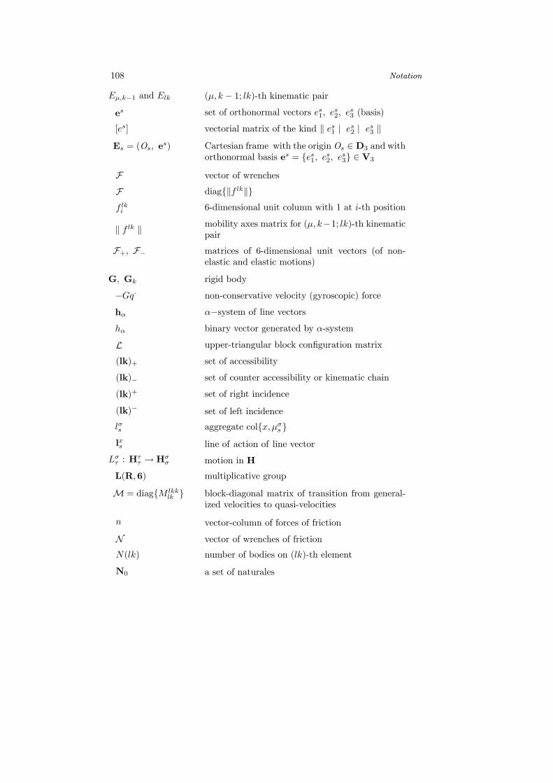
108 Notation
Eµ,k−1 and Elk (µ, k − 1; lk)-th kinematic pair
es set of orthonormal vectors es1, es2, e
s3 (basis)
[es] vectorial matrix of the kind k es1 | es2 | es3 k
Es = (Os, es) Cartesian frame with the origin Os ∈ D3 and with
orthonormal basis es = es1, es2, es3 ∈ V3
F vector of wrenches
F diagkf lkkf lki 6-dimensional unit column with 1 at i-th position
k f lk k mobility axes matrix for (µ, k−1; lk)-th kinematicpair
F+, F− matrices of 6-dimensional unit vectors (of non-elastic and elastic motions)
G, Gk rigid body
−Gq· non-conservative velocity (gyroscopic) force
hα α−system of line vectors
hα binary vector generated by α-system
L upper-triangular block configuration matrix
(lk)+ set of accessibility
(lk)− set of counter accessibility or kinematic chain
(lk)+ set of right incidence
(lk)− set of left incidence
lσs aggregate colx, µσs lxs line of action of line vector
Lστ : Hττ →Hσ
σ motion in H
L(R,6) multiplicative group
M = diagM lkklk block-diagonal matrix of transition from general-
ized velocities to quasi-velocities
n vector-column of forces of friction
N vector of wrenches of friction
N(lk) number of bodies on (lk)-th element
N0 a set of naturales

Notation 109
N×, N+ number of mulltiplications, additions
ost ∈ V3 vector of translation of Et to Es
oµ,k−1lk translation
0 = (0, 0, 0) 3-dimensional null row
−−−→(O , a) the bounded vector with the initial point O and
the terminal one a
O ∈ D3 center of reduction
ps,k−1lkk column of constructive translations
plki constructive translation
P operation of permutation of matrix rows andcolumns
q∗, u∗ reference motion and control
q+, q− generalized coordinates of non-elastic (‘slow’) andelastic (‘fast’) motions
q· deriviative of q in time dqdt
qlki ∈ R1 generalized coordinate
qlk column of generalized coordinates of (µ, k−1; lk)-th kinematic pair
q· = col qlk. column of generalized velocities
Q0sGs kinetic binary vector in motion of G in E0 withrespect to Es
R vector of wrenches of internal reactions
Rµ,k−1lkconfiguration of (µ.k − 1; lk)-th kinematic pair
Rµ,k−1lkkconstructive configuration
Rlkklk functional configuration
S = FTMTL parastrophic matrix
Seo enlargement of S
SO(R,3) one− parameter group of matrices of rotationsst−αp rows of the parastrophic matrix ST st 6× 6-matrix of translation of Et to Es

110 Notation
tij(a) transvection
tj(b) diagonal matrix with b at place j and units at allother ones
ht, ki inner product
V sti = colvstti , wstti vector of quasi-velocities
V = colV i.j−1,njnj 6n-dimensional quasi-velocity column of all kine-matic pairs
V = colV 10;lklk 6n-dimensional quasi-velocity column of all (lk)-thelements
W sti = colwstti , vstti twist of motion of Et with respect to Es reduced
to the origin of Ei
W vector of wrenches of actions from externalmedium to system bodies
u vector-column of control forces u(µ, k−1; lk) alongaxes of motion of pairs (µ, k − 1; lk)
U vector of control wrenches
X ST.q·
χG characteristic function of points of D3 being occu-pied by G
Λlklk matrix of apparent additional masses of Glk
φlki constructive rotation
Φ block-diagonal matrix of quasi-velocities
θlki angle
θss inertia matrix of G with respect to 0s in es
Θ00,Θss Mises (inertia) matrices
Θlklk Mises matrix of Glk in Elk calculated at Olk andin elk