Agilent

Digital Modulation inCommunications Systems —

An IntroductionApplication Note 1298

2

This application note introduces the concepts ofdigital modulation used in many communicationssystems today. Emphasis is placed on explainingthe tradeoffs that are made to optimize efficienciesin system design.

Most communications systems fall into one of threecategories: bandwidth efficient, power efficient, orcost efficient. Bandwidth efficiency describes theability of a modulation scheme to accommodatedata within a limited bandwidth. Power efficiencydescribes the ability of the system to reliably sendinformation at the lowest practical power level. In most systems, there is a high priority on band-width efficiency. The parameter to be optimizeddepends on the demands of the particular system,as can be seen in the following two examples.

For designers of digital terrestrial microwaveradios, their highest priority is good bandwidthefficiency with low bit-error-rate. They have plentyof power available and are not concerned withpower efficiency. They are not especially con-cerned with receiver cost or complexity becausethey do not have to build large numbers of them.

On the other hand, designers of hand-held cellularphones put a high priority on power efficiencybecause these phones need to run on a battery.Cost is also a high priority because cellular phonesmust be low-cost to encourage more users. Accord-ingly, these systems sacrifice some bandwidth efficiency to get power and cost efficiency.

Every time one of these efficiency parameters(bandwidth, power, or cost) is increased, anotherone decreases, becomes more complex, or does notperform well in a poor environment. Cost is a dom-inant system priority. Low-cost radios will alwaysbe in demand. In the past, it was possible to makea radio low-cost by sacrificing power and band-width efficiency. This is no longer possible. Theradio spectrum is very valuable and operators whodo not use the spectrum efficiently could lose theirexisting licenses or lose out in the competition fornew ones. These are the tradeoffs that must beconsidered in digital RF communications design.

This application note covers

• the reasons for the move to digital modulation;• how information is modulated onto in-phase (I)

and quadrature (Q) signals; • different types of digital modulation;• filtering techniques to conserve bandwidth; • ways of looking at digitally modulated signals;• multiplexing techniques used to share the

transmission channel;• how a digital transmitter and receiver work;• measurements on digital RF communications

systems;• an overview table with key specifications for

the major digital communications systems; and • a glossary of terms used in digital RF communi-

cations.

These concepts form the building blocks of anycommunications system. If you understand thebuilding blocks, then you will be able to under-stand how any communications system, present or future, works.

Introduction

3

556

7

778

89

101011

1212121314141515161718192021

2222232324252627

28

29293031

1. Why Digital Modulation?1.1 Trading off simplicity and bandwidth1.2 Industry trends

2. Using I/Q Modulation (Amplitude and Phase Control) to Convey Information

2.1 Transmitting information2.2 Signal characteristics that can be modified2.3 Polar display—magnitude and phase represented

together2.4 Signal changes or modifications in polar form2.5 I/Q formats2.6 I and Q in a radio transmitter2.7 I and Q in a radio receiver2.8 Why use I and Q?

3. Digital Modulation Types and Relative Efficiencies3.1 Applications

3.1.1 Bit rate and symbol rate3.1.2 Spectrum (bandwidth) requirements3.1.3 Symbol clock

3.2 Phase Shift Keying (PSK)3.3 Frequency Shift Keying3.4 Minimum Shift Keying (MSK)3.5 Quadrature Amplitude Modulation (QAM)3.6 Theoretical bandwidth efficiency limits3.7 Spectral efficiency examples in practical radios3.8 I/Q offset modulation3.9 Differential modulation3.10 Constant amplitude modulation

4. Filtering4.1 Nyquist or raised cosine filter4.2 Transmitter-receiver matched filters4.3 Gaussian filter4.4 Filter bandwidth parameter alpha 4.5 Filter bandwidth effects4.6 Chebyshev equiripple FIR (finite impulse response) filter4.7 Spectral efficiency versus power consumption

5. Different Ways of Looking at a Digitally Modulated Signal Time and Frequency Domain View

5.1 Power and frequency view5.2 Constellation diagrams5.3 Eye diagrams5.4 Trellis diagrams

Table of Contents

4

32323233333434

353536

37373738383939394041414243

43

44

46

6. Sharing the Channel6.1 Multiplexing—frequency6.2 Multiplexing—time6.3 Multiplexing—code6.4 Multiplexing—geography6.5 Combining multiplexing modes6.6 Penetration versus efficiency

7. How Digital Transmitters and Receivers Work7.1 A digital communications transmitter7.2 A digital communications receiver

8. Measurements on Digital RF Communications Systems8.1 Power measurements

8.1.1 Adjacent Channel Power8.2 Frequency measurements

8.2.1 Occupied bandwidth8.3 Timing measurements8.4 Modulation accuracy8.5 Understanding Error Vector Magnitude (EVM)8.6 Troubleshooting with error vector measurements8.7 Magnitude versus phase error8.8 I/Q phase error versus time8.9 Error Vector Magnitude versus time8.10 Error spectrum (EVM versus frequency)

9. Summary

10. Overview of Communications Systems

11. Glossary of Terms

Table of Contents (continued)

5

The move to digital modulation provides moreinformation capacity, compatibility with digitaldata services, higher data security, better qualitycommunications, and quicker system availability.Developers of communications systems face theseconstraints:

• available bandwidth • permissible power • inherent noise level of the system

The RF spectrum must be shared, yet every daythere are more users for that spectrum as demandfor communications services increases. Digitalmodulation schemes have greater capacity to con-vey large amounts of information than analog mod-ulation schemes.

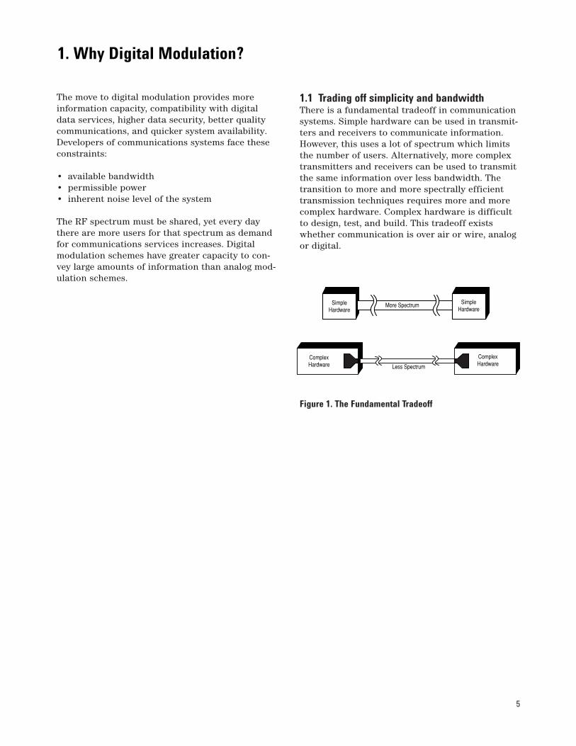
1.1 Trading off simplicity and bandwidthThere is a fundamental tradeoff in communicationsystems. Simple hardware can be used in transmit-ters and receivers to communicate information.However, this uses a lot of spectrum which limitsthe number of users. Alternatively, more complextransmitters and receivers can be used to transmitthe same information over less bandwidth. Thetransition to more and more spectrally efficienttransmission techniques requires more and morecomplex hardware. Complex hardware is difficultto design, test, and build. This tradeoff existswhether communication is over air or wire, analogor digital.

Figure 1. The Fundamental Tradeoff

ComplexHardware Less Spectrum

SimpleHardware

SimpleHardware

ComplexHardware

More Spectrum

1. Why Digital Modulation?

6

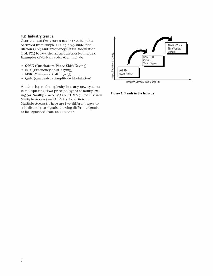
1.2 Industry trendsOver the past few years a major transition hasoccurred from simple analog Amplitude Mod-ulation (AM) and Frequency/Phase Modulation(FM/PM) to new digital modulation techniques.Examples of digital modulation include

• QPSK (Quadrature Phase Shift Keying) • FSK (Frequency Shift Keying)• MSK (Minimum Shift Keying)• QAM (Quadrature Amplitude Modulation)

Another layer of complexity in many new systemsis multiplexing. Two principal types of multiplex-ing (or “multiple access”) are TDMA (Time DivisionMultiple Access) and CDMA (Code DivisionMultiple Access). These are two different ways toadd diversity to signals allowing different signalsto be separated from one another.

QAM, FSK,QPSKVector Signals

AM, FMScalar Signals

TDMA, CDMATime-VariantSignals

Required Measurement Capability

Sign

al/S

yste

m C

ompl

exity

Figure 2. Trends in the Industry

7

2.1 Transmitting informationTo transmit a signal over the air, there are threemain steps:

1. A pure carrier is generated at the transmitter. 2. The carrier is modulated with the information

to be transmitted. Any reliably detectablechange in signal characteristics can carry information.

3. At the receiver the signal modifications orchanges are detected and demodulated.

2.2 Signal characteristics that can be modifiedThere are only three characteristics of a signal thatcan be changed over time: amplitude, phase, or fre-quency. However, phase and frequency are just dif-ferent ways to view or measure the same signalchange.

In AM, the amplitude of a high-frequency carriersignal is varied in proportion to the instantaneousamplitude of the modulating message signal.

Frequency Modulation (FM) is the most popularanalog modulation technique used in mobile com-munications systems. In FM, the amplitude of themodulating carrier is kept constant while its fre-quency is varied by the modulating message signal.

Amplitude and phase can be modulated simultane-ously and separately, but this is difficult to gener-ate, and especially difficult to detect. Instead, inpractical systems the signal is separated intoanother set of independent components: I (In-phase) and Q (Quadrature). These components areorthogonal and do not interfere with each other.

Modify aSignal

"Modulate"

Detect the Modifications "Demodulate"

Any reliably detectable change insignal characteristics can carry information

Amplitude

Frequency

or

Phase

Both Amplitude

and PhaseFigure 3. Transmitting Information (Analog or Digital)

Figure 4. Signal Characteristics to Modify

2. Using I/Q Modulation to Convey Information

8

2.3 Polar display—magnitude and phase repre-sented togetherA simple way to view amplitude and phase is withthe polar diagram. The carrier becomes a frequencyand phase reference and the signal is interpretedrelative to the carrier. The signal can be expressedin polar form as a magnitude and a phase. Thephase is relative to a reference signal, the carrierin most communication systems. The magnitude iseither an absolute or relative value. Both are usedin digital communication systems. Polar diagramsare the basis of many displays used in digital com-munications, although it is common to describe thesignal vector by its rectangular coordinates of I(In-phase) and Q (Quadrature).

2.4 Signal changes or modifications in polar formFigure 6 shows different forms of modulation inpolar form. Magnitude is represented as the dis-tance from the center and phase is represented asthe angle.

Amplitude modulation (AM) changes only the magnitude of the signal. Phase modulation (PM)changes only the phase of the signal. Amplitudeand phase modulation can be used together.Frequency modulation (FM) looks similar to phasemodulation, though frequency is the controlledparameter, rather than relative phase.

Phase

Mag

0 deg

Figure 5. Polar Display—Magnitude and PhaseRepresented Together

Phase

Mag

0 deg

Magnitude Change

Phase0 deg

Phase Change

Frequency Change Magnitude & Phase Change

0 deg

0 deg

Figure 6. Signal Changes or Modifications

9

One example of the difficulties in RF design can be illustrated with simple amplitude modulation.Generating AM with no associated angular modula-tion should result in a straight line on a polar display. This line should run from the origin tosome peak radius or amplitude value. In practice,however, the line is not straight. The amplitudemodulation itself often can cause a small amountof unwanted phase modulation. The result is acurved line. It could also be a loop if there is anyhysteresis in the system transfer function. Someamount of this distortion is inevitable in any sys-tem where modulation causes amplitude changes.

Therefore, the degree of effective amplitude modu-lation in a system will affect some distortionparameters.

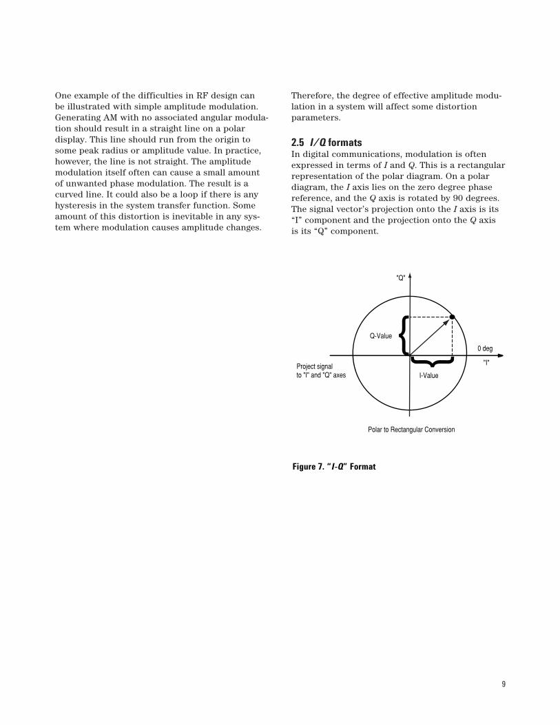
2.5 I/Q formatsIn digital communications, modulation is oftenexpressed in terms of I and Q. This is a rectangularrepresentation of the polar diagram. On a polardiagram, the I axis lies on the zero degree phasereference, and the Q axis is rotated by 90 degrees.The signal vector’s projection onto the I axis is its“I” component and the projection onto the Q axis is its “Q” component.

{ { 0 deg

"I"

"Q"

Q-Value

I-ValueProject signalto "I" and "Q" axes

Polar to Rectangular Conversion

Figure 7. “I-Q” Format

10

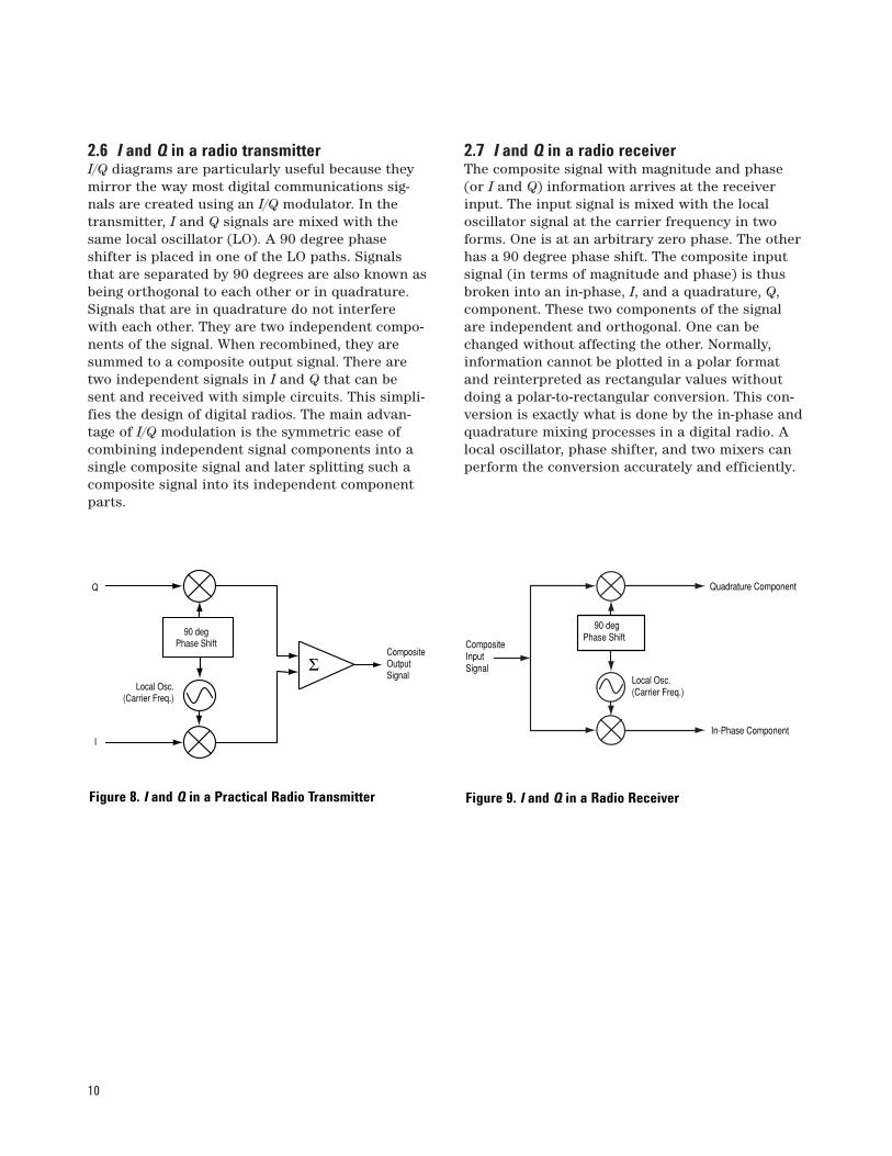
2.6 I and Q in a radio transmitterI/Q diagrams are particularly useful because theymirror the way most digital communications sig-nals are created using an I/Q modulator. In thetransmitter, I and Q signals are mixed with thesame local oscillator (LO). A 90 degree phaseshifter is placed in one of the LO paths. Signalsthat are separated by 90 degrees are also known asbeing orthogonal to each other or in quadrature.Signals that are in quadrature do not interferewith each other. They are two independent compo-nents of the signal. When recombined, they aresummed to a composite output signal. There aretwo independent signals in I and Q that can besent and received with simple circuits. This simpli-fies the design of digital radios. The main advan-tage of I/Q modulation is the symmetric ease ofcombining independent signal components into asingle composite signal and later splitting such acomposite signal into its independent componentparts.

2.7 I and Q in a radio receiverThe composite signal with magnitude and phase(or I and Q) information arrives at the receiverinput. The input signal is mixed with the localoscillator signal at the carrier frequency in twoforms. One is at an arbitrary zero phase. The otherhas a 90 degree phase shift. The composite inputsignal (in terms of magnitude and phase) is thusbroken into an in-phase, I, and a quadrature, Q,component. These two components of the signalare independent and orthogonal. One can bechanged without affecting the other. Normally,information cannot be plotted in a polar formatand reinterpreted as rectangular values withoutdoing a polar-to-rectangular conversion. This con-version is exactly what is done by the in-phase andquadrature mixing processes in a digital radio. Alocal oscillator, phase shifter, and two mixers canperform the conversion accurately and efficiently.

90 deg Phase Shift

Local Osc.(Carrier Freq.)

Q

I

CompositeOutputSignal

ΣLocal Osc.(Carrier Freq.)

Quadrature Component

In-Phase Component

CompositeInputSignal

90 degPhase Shift

Figure 8. I and Q in a Practical Radio Transmitter Figure 9. I and Q in a Radio Receiver

11

2.8 Why use I and Q?Digital modulation is easy to accomplish with I/Qmodulators. Most digital modulation maps the datato a number of discrete points on the I/Q plane.These are known as constellation points. As the sig-nal moves from one point to another, simultaneousamplitude and phase modulation usually results.To accomplish this with an amplitude modulatorand a phase modulator is difficult and complex. Itis also impossible with a conventional phase modu-lator. The signal may, in principle, circle the originin one direction forever, necessitating infinite phaseshifting capability. Alternatively, simultaneous AMand Phase Modulation is easy with an I/Q modulator.The I and Q control signals are bounded, but infi-nite phase wrap is possible by properly phasingthe I and Q signals.

12

This section covers the main digital modulationformats, their main applications, relative spectralefficiencies, and some variations of the main modulation types as used in practical systems.Fortunately, there are a limited number of modula-tion types which form the building blocks of anysystem.

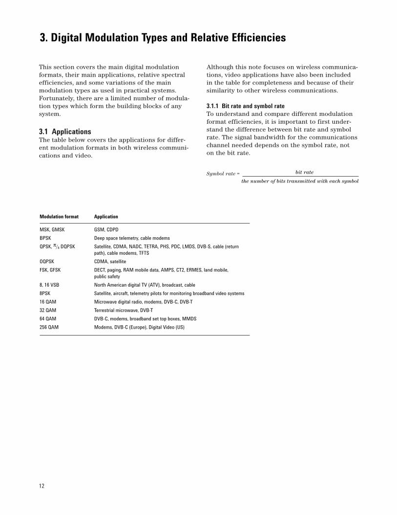
3.1 ApplicationsThe table below covers the applications for differ-ent modulation formats in both wireless communi-cations and video.

Although this note focuses on wireless communica-tions, video applications have also been includedin the table for completeness and because of theirsimilarity to other wireless communications.

3.1.1 Bit rate and symbol rateTo understand and compare different modulationformat efficiencies, it is important to first under-stand the difference between bit rate and symbolrate. The signal bandwidth for the communicationschannel needed depends on the symbol rate, noton the bit rate.

Symbol rate =

Modulation format Application

MSK, GMSK GSM, CDPD

BPSK Deep space telemetry, cable modems

QPSK, π/4 DQPSK Satellite, CDMA, NADC, TETRA, PHS, PDC, LMDS, DVB-S, cable (returnpath), cable modems, TFTS

OQPSK CDMA, satellite

FSK, GFSK DECT, paging, RAM mobile data, AMPS, CT2, ERMES, land mobile, public safety

8, 16 VSB North American digital TV (ATV), broadcast, cable

8PSK Satellite, aircraft, telemetry pilots for monitoring broadband video systems

16 QAM Microwave digital radio, modems, DVB-C, DVB-T

32 QAM Terrestrial microwave, DVB-T

64 QAM DVB-C, modems, broadband set top boxes, MMDS

256 QAM Modems, DVB-C (Europe), Digital Video (US)

bit rate

the number of bits transmitted with each symbol

3. Digital Modulation Types and Relative Efficiencies

13

Bit rate is the frequency of a system bit stream.Take, for example, a radio with an 8 bit sampler,sampling at 10 kHz for voice. The bit rate, the basicbit stream rate in the radio, would be eight bitsmultiplied by 10K samples per second, or 80 Kbitsper second. (For the moment we will ignore theextra bits required for synchronization, error correction, etc.)

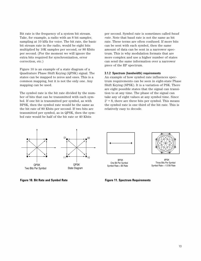
Figure 10 is an example of a state diagram of aQuadrature Phase Shift Keying (QPSK) signal. Thestates can be mapped to zeros and ones. This is acommon mapping, but it is not the only one. Anymapping can be used.

The symbol rate is the bit rate divided by the num-ber of bits that can be transmitted with each sym-bol. If one bit is transmitted per symbol, as withBPSK, then the symbol rate would be the same asthe bit rate of 80 Kbits per second. If two bits aretransmitted per symbol, as in QPSK, then the sym-bol rate would be half of the bit rate or 40 Kbits

per second. Symbol rate is sometimes called baudrate. Note that baud rate is not the same as bitrate. These terms are often confused. If more bitscan be sent with each symbol, then the sameamount of data can be sent in a narrower spec-trum. This is why modulation formats that aremore complex and use a higher number of statescan send the same information over a narrowerpiece of the RF spectrum.

3.1.2 Spectrum (bandwidth) requirementsAn example of how symbol rate influences spec-trum requirements can be seen in eight-state PhaseShift Keying (8PSK). It is a variation of PSK. Thereare eight possible states that the signal can transi-tion to at any time. The phase of the signal cantake any of eight values at any symbol time. Since23 = 8, there are three bits per symbol. This meansthe symbol rate is one third of the bit rate. This isrelatively easy to decode.

01 00

1011

QPSKTwo Bits Per Symbol

QPSKState Diagram

BPSKOne Bit Per Symbol

Symbol Rate = Bit Rate

8PSKThree Bits Per Symbol

Symbol Rate = 1/3 Bit Rate

Figure 10. Bit Rate and Symbol Rate Figure 11. Spectrum Requirements

3.1.3 Symbol ClockThe symbol clock represents the frequency andexact timing of the transmission of the individualsymbols. At the symbol clock transitions, the trans-mitted carrier is at the correct I/Q (or magnitude/phase) value to represent a specific symbol (a specific point in the constellation).

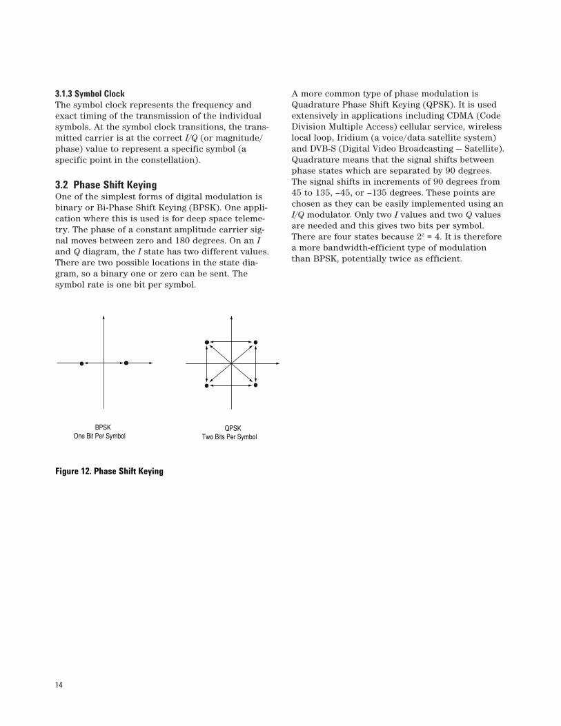
3.2 Phase Shift KeyingOne of the simplest forms of digital modulation isbinary or Bi-Phase Shift Keying (BPSK). One appli-cation where this is used is for deep space teleme-try. The phase of a constant amplitude carrier sig-nal moves between zero and 180 degrees. On an Iand Q diagram, the I state has two different values.There are two possible locations in the state dia-gram, so a binary one or zero can be sent. Thesymbol rate is one bit per symbol.

A more common type of phase modulation isQuadrature Phase Shift Keying (QPSK). It is usedextensively in applications including CDMA (CodeDivision Multiple Access) cellular service, wirelesslocal loop, Iridium (a voice/data satellite system)and DVB-S (Digital Video Broadcasting — Satellite).Quadrature means that the signal shifts betweenphase states which are separated by 90 degrees.The signal shifts in increments of 90 degrees from45 to 135, –45, or –135 degrees. These points arechosen as they can be easily implemented using anI/Q modulator. Only two I values and two Q valuesare needed and this gives two bits per symbol.There are four states because 22 = 4. It is thereforea more bandwidth-efficient type of modulationthan BPSK, potentially twice as efficient.

14

BPSKOne Bit Per Symbol

QPSKTwo Bits Per Symbol

Figure 12. Phase Shift Keying

15

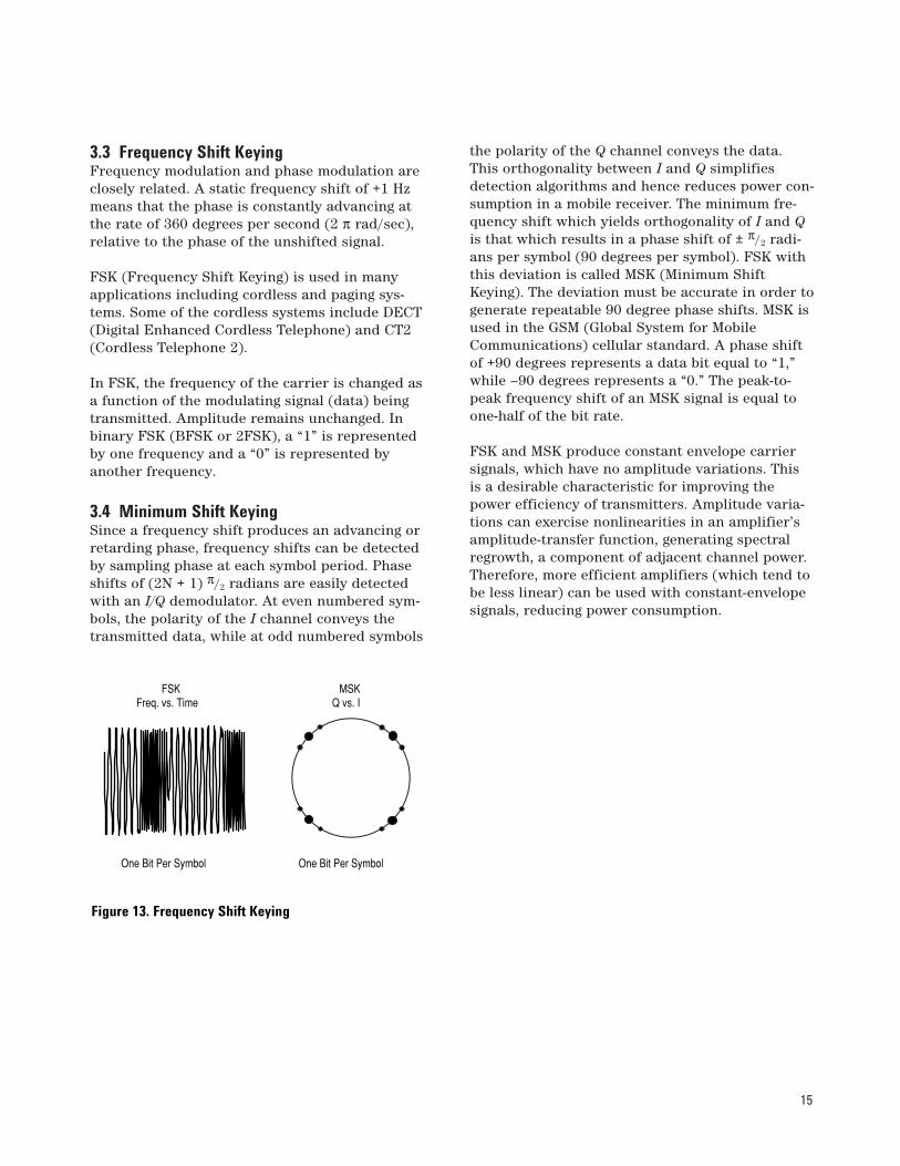
3.3 Frequency Shift KeyingFrequency modulation and phase modulation areclosely related. A static frequency shift of +1 Hzmeans that the phase is constantly advancing atthe rate of 360 degrees per second (2 π rad/sec),relative to the phase of the unshifted signal.

FSK (Frequency Shift Keying) is used in manyapplications including cordless and paging sys-tems. Some of the cordless systems include DECT(Digital Enhanced Cordless Telephone) and CT2(Cordless Telephone 2).

In FSK, the frequency of the carrier is changed asa function of the modulating signal (data) beingtransmitted. Amplitude remains unchanged. Inbinary FSK (BFSK or 2FSK), a “1” is representedby one frequency and a “0” is represented byanother frequency.

3.4 Minimum Shift KeyingSince a frequency shift produces an advancing orretarding phase, frequency shifts can be detectedby sampling phase at each symbol period. Phaseshifts of (2N + 1) π/2 radians are easily detectedwith an I/Q demodulator. At even numbered sym-bols, the polarity of the I channel conveys thetransmitted data, while at odd numbered symbols

the polarity of the Q channel conveys the data.This orthogonality between I and Q simplifiesdetection algorithms and hence reduces power con-sumption in a mobile receiver. The minimum fre-quency shift which yields orthogonality of I and Qis that which results in a phase shift of ± π/2 radi-ans per symbol (90 degrees per symbol). FSK withthis deviation is called MSK (Minimum ShiftKeying). The deviation must be accurate in order togenerate repeatable 90 degree phase shifts. MSK isused in the GSM (Global System for MobileCommunications) cellular standard. A phase shiftof +90 degrees represents a data bit equal to “1,”while –90 degrees represents a “0.” The peak-to-peak frequency shift of an MSK signal is equal toone-half of the bit rate.

FSK and MSK produce constant envelope carriersignals, which have no amplitude variations. Thisis a desirable characteristic for improving thepower efficiency of transmitters. Amplitude varia-tions can exercise nonlinearities in an amplifier’samplitude-transfer function, generating spectralregrowth, a component of adjacent channel power.Therefore, more efficient amplifiers (which tend tobe less linear) can be used with constant-envelopesignals, reducing power consumption.

MSKQ vs. I

FSKFreq. vs. Time

One Bit Per Symbol One Bit Per Symbol

Figure 13. Frequency Shift Keying

16

MSK has a narrower spectrum than wider devia-tion forms of FSK. The width of the spectrum isalso influenced by the waveforms causing the fre-quency shift. If those waveforms have fast transi-tions or a high slew rate, then the spectrum of the transmitter will be broad. In practice, thewaveforms are filtered with a Gaussian filter,resulting in a narrow spectrum. In addition, theGaussian filter has no time-domain overshoot,which would broaden the spectrum by increasingthe peak deviation. MSK with a Gaussian filter istermed GMSK (Gaussian MSK).

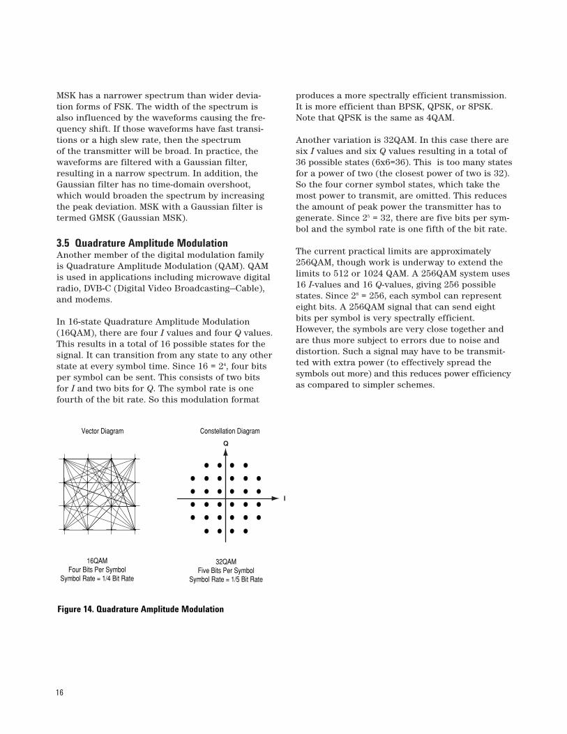
3.5 Quadrature Amplitude ModulationAnother member of the digital modulation familyis Quadrature Amplitude Modulation (QAM). QAMis used in applications including microwave digitalradio, DVB-C (Digital Video Broadcasting—Cable),and modems.

In 16-state Quadrature Amplitude Modulation(16QAM), there are four I values and four Q values.This results in a total of 16 possible states for thesignal. It can transition from any state to any otherstate at every symbol time. Since 16 = 24, four bitsper symbol can be sent. This consists of two bitsfor I and two bits for Q. The symbol rate is onefourth of the bit rate. So this modulation format

produces a more spectrally efficient transmission.It is more efficient than BPSK, QPSK, or 8PSK.Note that QPSK is the same as 4QAM.

Another variation is 32QAM. In this case there aresix I values and six Q values resulting in a total of36 possible states (6x6=36). This is too many statesfor a power of two (the closest power of two is 32).So the four corner symbol states, which take themost power to transmit, are omitted. This reducesthe amount of peak power the transmitter has togenerate. Since 25 = 32, there are five bits per sym-bol and the symbol rate is one fifth of the bit rate.

The current practical limits are approximately256QAM, though work is underway to extend thelimits to 512 or 1024 QAM. A 256QAM system uses16 I-values and 16 Q-values, giving 256 possiblestates. Since 28 = 256, each symbol can representeight bits. A 256QAM signal that can send eightbits per symbol is very spectrally efficient.However, the symbols are very close together andare thus more subject to errors due to noise anddistortion. Such a signal may have to be transmit-ted with extra power (to effectively spread thesymbols out more) and this reduces power efficiencyas compared to simpler schemes.

16QAMFour Bits Per Symbol

Symbol Rate = 1/4 Bit Rate

I

Q

32QAMFive Bits Per Symbol

Symbol Rate = 1/5 Bit Rate

Vector Diagram Constellation Diagram

Figure 14. Quadrature Amplitude Modulation

17

Compare the bandwidth efficiency when using256QAM versus BPSK modulation in the radioexample in section 3.1.1 (which uses an eight-bitsampler sampling at 10 kHz for voice). BPSK uses80 Ksymbols-per-second sending 1 bit per symbol.A system using 256QAM sends eight bits per sym-bol so the symbol rate would be 10 Ksymbols persecond. A 256QAM system enables the sameamount of information to be sent as BPSK usingonly one eighth of the bandwidth. It is eight timesmore bandwidth efficient. However, there is atradeoff. The radio becomes more complex and ismore susceptible to errors caused by noise and dis-tortion. Error rates of higher-order QAM systemssuch as this degrade more rapidly than QPSK asnoise or interference is introduced. A measure of this degradation would be a higher Bit ErrorRate (BER).

In any digital modulation system, if the input sig-nal is distorted or severely attenuated the receiverwill eventually lose symbol lock completely. If thereceiver can no longer recover the symbol clock, itcannot demodulate the signal or recover any infor-mation. With less degradation, the symbol clockcan be recovered, but it is noisy, and the symbollocations themselves are noisy. In some cases, asymbol will fall far enough away from its intendedposition that it will cross over to an adjacent posi-tion. The I and Q level detectors used in thedemodulator would misinterpret such a symbol asbeing in the wrong location, causing bit errors.QPSK is not as efficient, but the states are much

farther apart and the system can tolerate a lotmore noise before suffering symbol errors. QPSKhas no intermediate states between the four corner-symbol locations, so there is less opportunityfor the demodulator to misinterpret symbols. QPSK requires less transmitter power than QAM to achieve the same bit error rate.

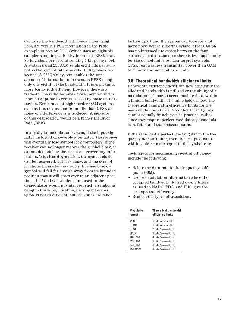
3.6 Theoretical bandwidth efficiency limitsBandwidth efficiency describes how efficiently theallocated bandwidth is utilized or the ability of amodulation scheme to accommodate data, within a limited bandwidth. The table below shows thetheoretical bandwidth efficiency limits for themain modulation types. Note that these figurescannot actually be achieved in practical radiossince they require perfect modulators, demodula-tors, filter, and transmission paths.

If the radio had a perfect (rectangular in the fre-quency domain) filter, then the occupied band-width could be made equal to the symbol rate.

Techniques for maximizing spectral efficiencyinclude the following:

• Relate the data rate to the frequency shift (as in GSM).

• Use premodulation filtering to reduce the occupied bandwidth. Raised cosine filters, as used in NADC, PDC, and PHS, give the best spectral efficiency.

• Restrict the types of transitions.

Modulation Theoretical bandwidth format efficiency limits

MSK 1 bit/second/Hz BPSK 1 bit/second/Hz QPSK 2 bits/second/Hz 8PSK 3 bits/second/Hz 16 QAM 4 bits/second/Hz 32 QAM 5 bits/second/Hz 64 QAM 6 bits/second/Hz 256 QAM 8 bits/second/Hz

18

Effects of going through the originTake, for example, a QPSK signal where the normalizedvalue changes from 1, 1 to –1, –1. When changing simulta-neously from I and Q values of +1 to I and Q values of –1,the signal trajectory goes through the origin (the I/Q valueof 0,0). The origin represents 0 carrier magnitude. A valueof 0 magnitude indicates that the carrier amplitude is 0 fora moment.

Not all transitions in QPSK result in a trajectory that goesthrough the origin. If I changes value but Q does not (orvice-versa) the carrier amplitude changes a little, but itdoes not go through zero. Therefore some symbol transi-tions will result in a small amplitude variation, while otherswill result in a very large amplitude variation. The clock-recovery circuit in the receiver must deal with this ampli-tude variation uncertainty if it uses amplitude variations to align the receiver clock with the transmitter clock.

Spectral regrowth does not automatically result from thesetrajectories that pass through or near the origin. If theamplifier and associated circuits are perfectly linear, thespectrum (spectral occupancy or occupied bandwidth) willbe unchanged. The problem lies in nonlinearities in the circuits.

A signal which changes amplitude over a very large rangewill exercise these nonlinearities to the fullest extent.These nonlinearities will cause distortion products. In con-tinuously modulated systems they will cause “spectralregrowth” or wider modulation sidebands (a phenomenonrelated to intermodulation distortion). Another term whichis sometimes used in this context is “spectral splatter.”However this is a term that is more correctly used in asso-ciation with the increase in the bandwidth of a signalcaused by pulsing on and off.

3.7 Spectral efficiency examples in practical radiosThe following examples indicate spectral efficien-cies that are achieved in some practical radio systems.

The TDMA version of the North American DigitalCellular (NADC) system, achieves a 48 Kbits-per-second data rate over a 30 kHz bandwidth or 1.6 bitsper second per Hz. It is a π/4 DQPSK based systemand transmits two bits per symbol. The theoreticalefficiency would be two bits per second per Hz andin practice it is 1.6 bits per second per Hz.

Another example is a microwave digital radio using16QAM. This kind of signal is more susceptible tonoise and distortion than something simpler suchas QPSK. This type of signal is usually sent over adirect line-of-sight microwave link or over a wirewhere there is very little noise and interference. Inthis microwave-digital-radio example the bit rate is140 Mbits per second over a very wide bandwidthof 52.5 MHz. The spectral efficiency is 2.7 bits persecond per Hz. To implement this, it takes a veryclear line-of-sight transmission path and a preciseand optimized high-power transceiver.

19

Digital modulation types—variationsThe modulation types outlined in sections 3.2 to3.4 form the building blocks for many systems.There are three main variations on these basicbuilding blocks that are used in communicationssystems: I/Q offset modulation, differential modula-tion, and constant envelope modulation.

3.8 I/Q offset modulationThe first variation is offset modulation. One exam-ple of this is Offset QPSK (OQPSK). This is used inthe cellular CDMA (Code Division Multiple Access)system for the reverse (mobile to base) link.

In QPSK, the I and Q bit streams are switched atthe same time. The symbol clocks, or the I and Qdigital signal clocks, are synchronized. In Offset

QPSK (OQPSK), the I and Q bit streams are offsetin their relative alignment by one bit period (onehalf of a symbol period). This is shown in the dia-gram. Since the transitions of I and Q are offset, atany given time only one of the two bit streams canchange values. This creates a dramatically differentconstellation, even though there are still just twoI/Q values. This has power efficiency advantages.In OQPSK the signal trajectories are modified bythe symbol clock offset so that the carrier ampli-tude does not go through or near zero (the centerof the constellation). The spectral efficiency is thesame with two I states and two Q states. Thereduced amplitude variations (perhaps 3 dB forOQPSK, versus 30 to 40 dB for QPSK) allow a morepower-efficient, less linear RF power amplifier tobe used.

QPSK

OffsetQPSK

Q

I

Q

I

Eye Constellation

Figure 15. I-Q “Offset” Modulation

20

3.9 Differential modulationThe second variation is differential modulation asused in differential QPSK (DQPSK) and differential16QAM (D16QAM). Differential means that theinformation is not carried by the absolute state, itis carried by the transition between states. In somecases there are also restrictions on allowable tran-sitions. This occurs in π/4 DQPSK where the carriertrajectory does not go through the origin. A DQPSKtransmission system can transition from any sym-bol position to any other symbol position. The π/4

DQPSK modulation format is widely used in manyapplications including

• cellular–NADC- IS-54 (North American digital cellular)–PDC (Pacific Digital Cellular)

• cordless –PHS (personal handyphone system)

• trunked radio–TETRA (Trans European Trunked Radio)

The π/4 DQPSK modulation format uses two QPSKconstellations offset by 45 degrees (π/4 radians).Transitions must occur from one constellation tothe other. This guarantees that there is always achange in phase at each symbol, making clockrecovery easier. The data is encoded in the magni-tude and direction of the phase shift, not in theabsolute position on the constellation. One advan-tage of π/4 DQPSK is that the signal trajectory doesnot pass through the origin, thus simplifying trans-mitter design. Another is that π/4 DQPSK, with rootraised cosine filtering, has better spectral efficiencythan GMSK, the other common cellular modulationtype.

QPSK π/4 DQPSK

Both formats are 2 bits/symbol

Figure 16. Differential Modulation

21

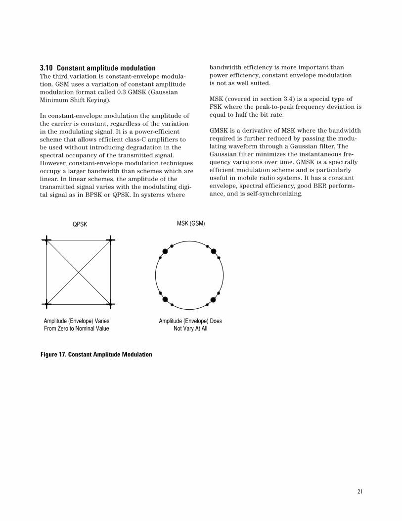
3.10 Constant amplitude modulationThe third variation is constant-envelope modula-tion. GSM uses a variation of constant amplitudemodulation format called 0.3 GMSK (GaussianMinimum Shift Keying).

In constant-envelope modulation the amplitude ofthe carrier is constant, regardless of the variationin the modulating signal. It is a power-efficientscheme that allows efficient class-C amplifiers tobe used without introducing degradation in thespectral occupancy of the transmitted signal.However, constant-envelope modulation techniquesoccupy a larger bandwidth than schemes which arelinear. In linear schemes, the amplitude of thetransmitted signal varies with the modulating digi-tal signal as in BPSK or QPSK. In systems where

bandwidth efficiency is more important thanpower efficiency, constant envelope modulation is not as well suited.

MSK (covered in section 3.4) is a special type ofFSK where the peak-to-peak frequency deviation isequal to half the bit rate.

GMSK is a derivative of MSK where the bandwidthrequired is further reduced by passing the modu-lating waveform through a Gaussian filter. TheGaussian filter minimizes the instantaneous fre-quency variations over time. GMSK is a spectrallyefficient modulation scheme and is particularlyuseful in mobile radio systems. It has a constantenvelope, spectral efficiency, good BER perform-ance, and is self-synchronizing.

MSK (GSM)

Amplitude (Envelope) VariesFrom Zero to Nominal Value

QPSK

Amplitude (Envelope) DoesNot Vary At All

Figure 17. Constant Amplitude Modulation

22

Filtering allows the transmitted bandwidth to besignificantly reduced without losing the content of the digital data. This improves the spectral effi-ciency of the signal.

There are many different varieties of filtering. The most common are

• raised cosine • square-root raised cosine• Gaussian filters

Any fast transition in a signal, whether it be ampli-tude, phase, or frequency, will require a wide occu-pied bandwidth. Any technique that helps to slowdown these transitions will narrow the occupiedbandwidth. Filtering serves to smooth these transi-tions (in I and Q). Filtering reduces interferencebecause it reduces the tendency of one signal orone transmitter to interfere with another in aFrequency-Division-Multiple-Access (FDMA) system.On the receiver end, reduced bandwidth improvessensitivity because more noise and interferenceare rejected.

Some tradeoffs must be made. One is that sometypes of filtering cause the trajectory of the signal(the path of transitions between the states) toovershoot in many cases. This overshoot can occurin certain types of filters such as Nyquist. This

overshoot path represents carrier power and phase.For the carrier to take on these values it requiresmore output power from the transmitter ampli-fiers. It requires more power than would be neces-sary to transmit the actual symbol itself. Carrierpower cannot be clipped or limited (to reduce oreliminate the overshoot) without causing the spec-trum to spread out again. Since narrowing thespectral occupancy was the reason the filteringwas inserted in the first place, it becomes a veryfine balancing act.

Other tradeoffs are that filtering makes the radiosmore complex and can make them larger, especiallyif performed in an analog fashion. Filtering canalso create Inter-Symbol Interference (ISI). Thisoccurs when the signal is filtered enough so thatthe symbols blur together and each symbol affectsthose around it. This is determined by the time-domain response or impulse response of the filter.

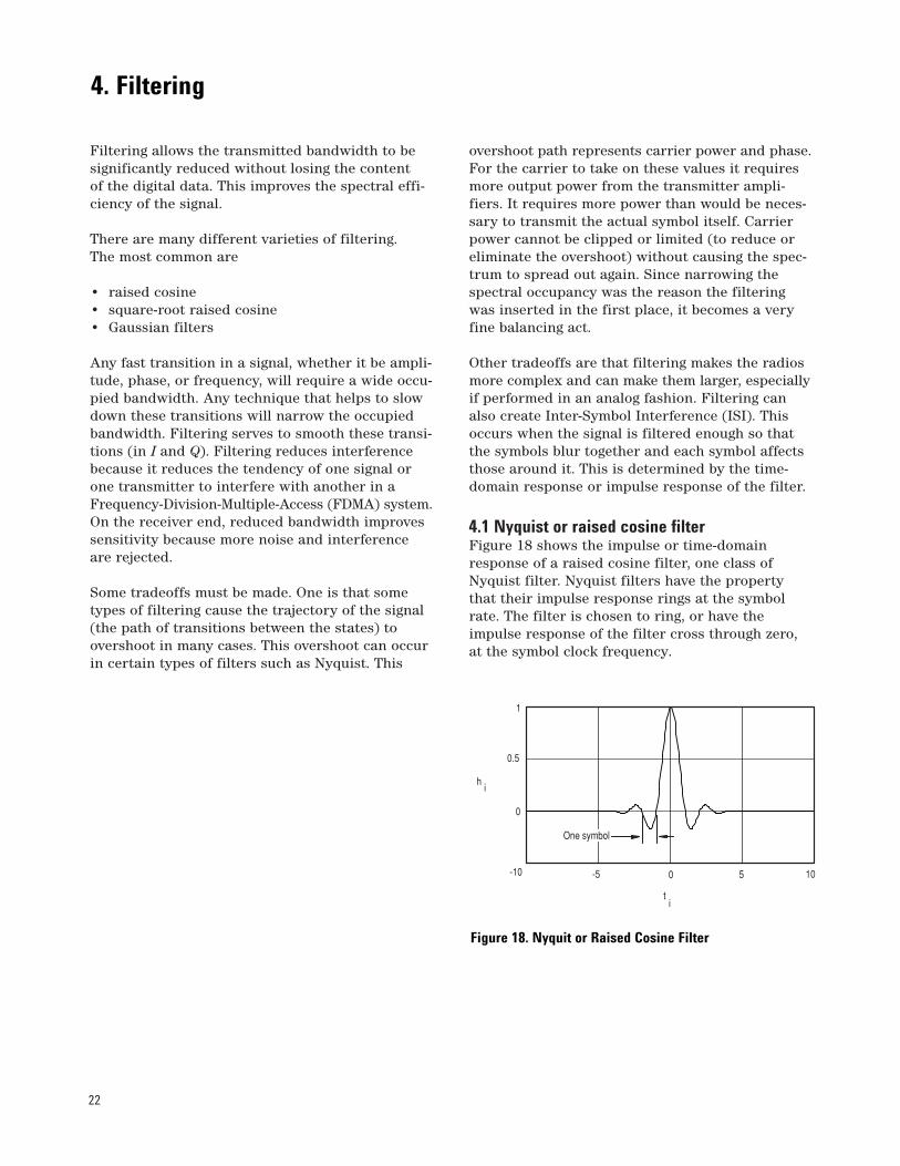
4.1 Nyquist or raised cosine filterFigure 18 shows the impulse or time-domainresponse of a raised cosine filter, one class ofNyquist filter. Nyquist filters have the propertythat their impulse response rings at the symbolrate. The filter is chosen to ring, or have theimpulse response of the filter cross through zero,at the symbol clock frequency.

0

0.5

1

-10 -5 0 5 10

hi

ti

One symbol

Figure 18. Nyquit or Raised Cosine Filter

4. Filtering

23

The time response of the filter goes through zerowith a period that exactly corresponds to the sym-bol spacing. Adjacent symbols do not interfere with each other at the symbol times because theresponse equals zero at all symbol times except thecenter (desired) one. Nyquist filters heavily filterthe signal without blurring the symbols togetherat the symbol times. This is important for transmit-ting information without errors caused by Inter-Symbol Interference. Note that Inter-SymbolInterference does exist at all times except the sym-bol (decision) times. Usually the filter is split, halfbeing in the transmit path and half in the receiverpath. In this case root Nyquist filters (commonlycalled root raised cosine) are used in each part, sothat their combined response is that of a Nyquistfilter.

4.2 Transmitter-receiver matched filtersSometimes filtering is desired at both the trans-mitter and receiver. Filtering in the transmitterreduces the adjacent-channel-power radiation ofthe transmitter, and thus its potential for interfer-ing with other transmitters.

Filtering at the receiver reduces the effects ofbroadband noise and also interference from othertransmitters in nearby channels.

To get zero Inter-Symbol Interference (ISI), bothfilters are designed until the combined result ofthe filters and the rest of the system is a full Nyquistfilter. Potential differences can cause problems inmanufacturing because the transmitter and receiverare often manufactured by different companies.The receiver may be a small hand-held model andthe transmitter may be a large cellular base sta-tion. If the design is performed correctly the resultsare the best data rate, the most efficient radio, andreduced effects of interference and noise. This iswhy root-Nyquist filters are used in receivers andtransmitters as √ Nyquist x √ Nyquist = Nyquist.Matched filters are not used in Gaussian filtering.

4.3 Gaussian filterIn contrast, a GSM signal will have a small blurringof symbols on each of the four states because theGaussian filter used in GSM does not have zeroInter-Symbol Interference. The phase states varysomewhat causing a blurring of the symbols, asshown in Figure 17. Wireless system architectsmust decide just how much of the Inter-SymbolInterference can be tolerated in a system and com-bine that with noise and interference.

Actual Data

Root RaisedCosine Filter

DAC

Detected Bits

Root RaisedCosine Filter

Transmitter

ReceiverDemodulator

Modulator

Figure 19. Transmitter-Receiver Matched Filters

24

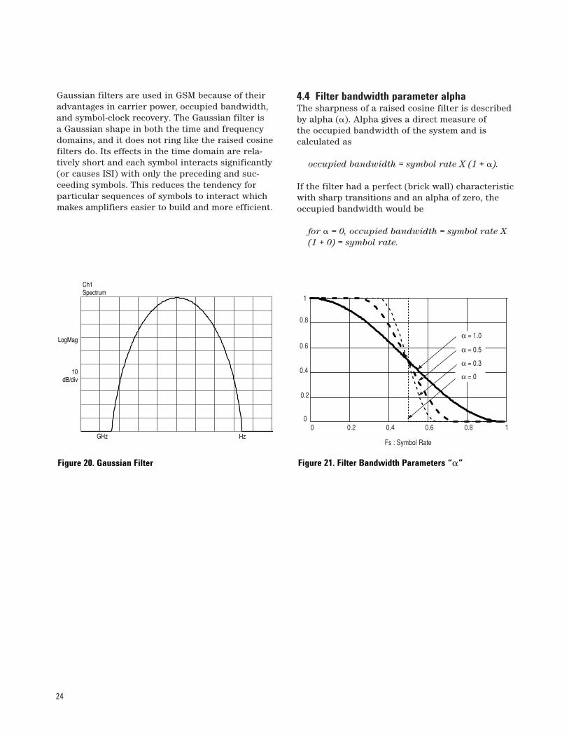
Gaussian filters are used in GSM because of theiradvantages in carrier power, occupied bandwidth,and symbol-clock recovery. The Gaussian filter is a Gaussian shape in both the time and frequencydomains, and it does not ring like the raised cosinefilters do. Its effects in the time domain are rela-tively short and each symbol interacts significantly(or causes ISI) with only the preceding and suc-ceeding symbols. This reduces the tendency forparticular sequences of symbols to interact whichmakes amplifiers easier to build and more efficient.

4.4 Filter bandwidth parameter alpha The sharpness of a raised cosine filter is describedby alpha (�). Alpha gives a direct measure of the occupied bandwidth of the system and is calculated as

occupied bandwidth = symbol rate X (1 + �).

If the filter had a perfect (brick wall) characteristicwith sharp transitions and an alpha of zero, theoccupied bandwidth would be

for � = 0, occupied bandwidth = symbol rate X (1 + 0) = symbol rate.

Hz

Ch1Spectrum

LogMag

10dB/div

GHz

0

0.2

0.4

0.6

0.8

1

0 0.2 0.4 0.6 0.8 1

α = 0.3

α = 0.5

α = 0

α = 1.0

Fs : Symbol Rate

Figure 20. Gaussian Filter Figure 21. Filter Bandwidth Parameters “�”

25

In a perfect world, the occupied bandwidth wouldbe the same as the symbol rate, but this is notpractical. An alpha of zero is impossible to implement.

Alpha is sometimes called the “excess bandwidthfactor” as it indicates the amount of occupiedbandwidth that will be required in excess of theideal occupied bandwidth (which would be thesame as the symbol rate).

At the other extreme, take a broader filter with analpha of one, which is easier to implement. Theoccupied bandwidth will be

for � = 1, occupied bandwidth = symbol rate X (1 + 1) = 2 X symbol rate.

An alpha of one uses twice as much bandwidth asan alpha of zero. In practice, it is possible to imple-ment an alpha below 0.2 and make good, compact,practical radios. Typical values range from 0.35 to0.5, though some video systems use an alpha aslow as 0.11. The corresponding term for a Gaussianfilter is BT (bandwidth time product). Occupiedbandwidth cannot be stated in terms of BT because

a Gaussian filter’s frequency response does not goidentically to zero, as does a raised cosine. Commonvalues for BT are 0.3 to 0.5.

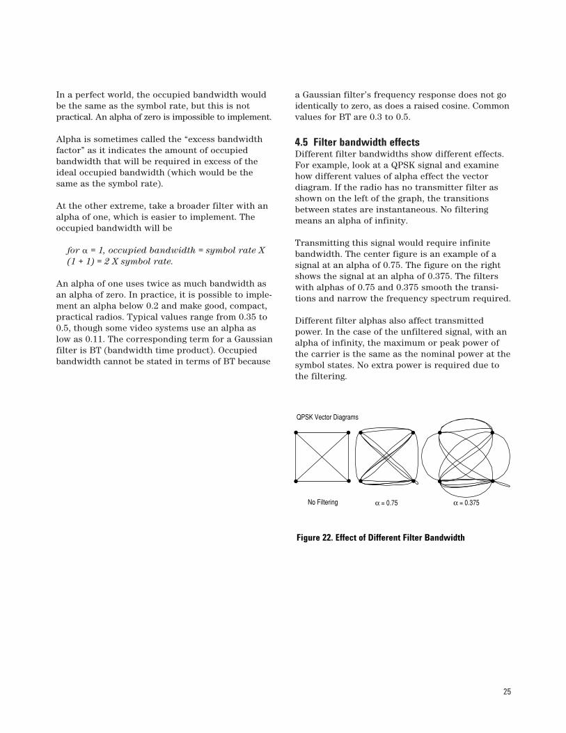
4.5 Filter bandwidth effectsDifferent filter bandwidths show different effects.For example, look at a QPSK signal and examinehow different values of alpha effect the vector diagram. If the radio has no transmitter filter asshown on the left of the graph, the transitionsbetween states are instantaneous. No filteringmeans an alpha of infinity.

Transmitting this signal would require infinitebandwidth. The center figure is an example of asignal at an alpha of 0.75. The figure on the rightshows the signal at an alpha of 0.375. The filterswith alphas of 0.75 and 0.375 smooth the transi-tions and narrow the frequency spectrum required.

Different filter alphas also affect transmittedpower. In the case of the unfiltered signal, with analpha of infinity, the maximum or peak power ofthe carrier is the same as the nominal power at thesymbol states. No extra power is required due tothe filtering.

QPSK Vector Diagrams

No Filtering α = 0.75 α = 0.375

Figure 22. Effect of Different Filter Bandwidth

26

Take an example of a π/4 DQPSK signal as used inNADC (IS-54). If an alpha of 1.0 is used, the transi-tions between the states are more gradual than foran alpha of infinity. Less power is needed to handlethose transitions. Using an alpha of 0.5, the trans-mitted bandwidth decreases from 2 times the sym-bol rate to 1.5 times the symbol rate. This resultsin a 25% improvement in occupied bandwidth. Thesmaller alpha takes more peak power because ofthe overshoot in the filter’s step response. Thisproduces trajectories which loop beyond the outerlimits of the constellation.

At an alpha of 0.2, about the minimum of mostradios today, there is a need for significant excesspower beyond that needed to transmit the symbolvalues themselves. A typical value of excess powerneeded at an alpha of 0.2 for QPSK with Nyquistfiltering would be approximately 5 dB. This is morethan three times as much peak power because ofthe filter used to limit the occupied bandwidth.

These principles apply to QPSK, offset QPSK,DQPSK, and the varieties of QAM such as 16QAM,32QAM, 64QAM, and 256QAM. Not all signals willbehave in exactly the same way, and exceptions

include FSK, MSK, and any others with constant-envelope modulation. The power of these signals is not affected by the filter shape.

4.6 Chebyshev equiripple FIR (finite impulserespone) filterA Chebyshev equiripple FIR (finite impulse response)filter is used for baseband filtering in IS-95 CDMA.With a channel spacing of 1.25 MHz and a symbolrate of 1.2288 MHz in IS-95 CDMA, it is vital toreduce leakage to adjacent RF channels. This isaccomplished by using a filter with a very sharpshape factor using an alpha value of only 0.113. AFIR filter means that the filter’s impulse responseexists for only a finite number of samples. Equi-ripple means that there is a “rippled” magnitudefrequency-respone envelope of equal maxima andminima in the pass- and stopbands. This FIR filteruses a much lower order than a Nyquist filter toimplement the required shape factor. The IS-95 FIRfilter does not have zero Inter Symbol Interference(ISI). However, ISI in CDMA is not as important asin other formats since the correlation of 64 chipsat a time is used to make a symbol decision. This“coding gain” tends to average out the ISI and min-imize its effect.

Figure 23. Chebyshev Equiripple FIR Filter

27

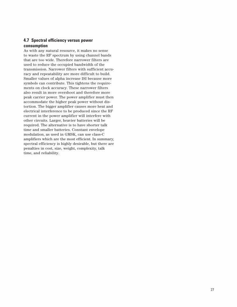
4.7 Spectral efficiency versus power consumptionAs with any natural resource, it makes no sense to waste the RF spectrum by using channel bandsthat are too wide. Therefore narrower filters areused to reduce the occupied bandwidth of thetransmission. Narrower filters with sufficient accu-racy and repeatability are more difficult to build.Smaller values of alpha increase ISI because moresymbols can contribute. This tightens the require-ments on clock accuracy. These narrower filtersalso result in more overshoot and therefore morepeak carrier power. The power amplifier must thenaccommodate the higher peak power without dis-tortion. The bigger amplifier causes more heat andelectrical interference to be produced since the RFcurrent in the power amplifier will interfere withother circuits. Larger, heavier batteries will berequired. The alternative is to have shorter talktime and smaller batteries. Constant envelopemodulation, as used in GMSK, can use class-Camplifiers which are the most efficient. In summary,spectral efficiency is highly desirable, but there arepenalties in cost, size, weight, complexity, talktime, and reliability.

28

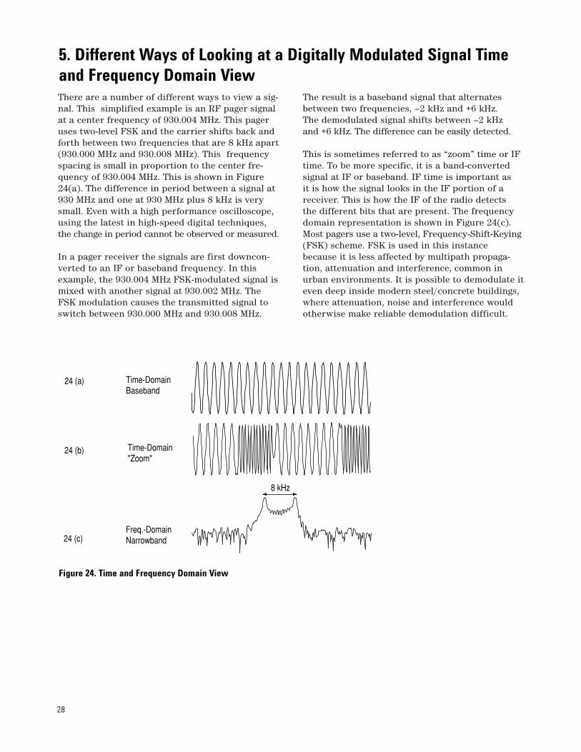
There are a number of different ways to view a sig-nal. This simplified example is an RF pager signalat a center frequency of 930.004 MHz. This pageruses two-level FSK and the carrier shifts back andforth between two frequencies that are 8 kHz apart(930.000 MHz and 930.008 MHz). This frequencyspacing is small in proportion to the center fre-quency of 930.004 MHz. This is shown in Figure 24(a). The difference in period between a signal at930 MHz and one at 930 MHz plus 8 kHz is verysmall. Even with a high performance oscilloscope,using the latest in high-speed digital techniques,the change in period cannot be observed or measured.

In a pager receiver the signals are first downcon-verted to an IF or baseband frequency. In thisexample, the 930.004 MHz FSK-modulated signal ismixed with another signal at 930.002 MHz. TheFSK modulation causes the transmitted signal toswitch between 930.000 MHz and 930.008 MHz.

The result is a baseband signal that alternatesbetween two frequencies, –2 kHz and +6 kHz. The demodulated signal shifts between –2 kHz and +6 kHz. The difference can be easily detected.

This is sometimes referred to as “zoom” time or IFtime. To be more specific, it is a band-convertedsignal at IF or baseband. IF time is important as it is how the signal looks in the IF portion of areceiver. This is how the IF of the radio detects the different bits that are present. The frequencydomain representation is shown in Figure 24(c).Most pagers use a two-level, Frequency-Shift-Keying(FSK) scheme. FSK is used in this instancebecause it is less affected by multipath propaga-tion, attenuation and interference, common inurban environments. It is possible to demodulate iteven deep inside modern steel/concrete buildings,where attenuation, noise and interference wouldotherwise make reliable demodulation difficult.

Time-DomainBaseband

Time-Domain"Zoom"

Freq.-DomainNarrowband

24 (a)

24 (c)

24 (b)

8 kHz

Figure 24. Time and Frequency Domain View

5. Different Ways of Looking at a Digitally Modulated Signal Timeand Frequency Domain View

29

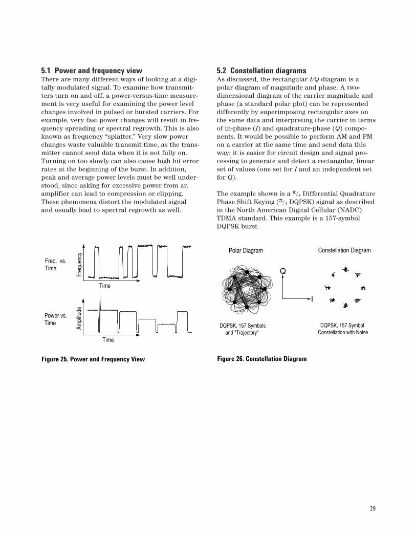
5.1 Power and frequency viewThere are many different ways of looking at a digi-tally modulated signal. To examine how transmit-ters turn on and off, a power-versus-time measure-ment is very useful for examining the power levelchanges involved in pulsed or bursted carriers. Forexample, very fast power changes will result in fre-quency spreading or spectral regrowth. This is alsoknown as frequency “splatter.” Very slow powerchanges waste valuable transmit time, as the trans-mitter cannot send data when it is not fully on.Turning on too slowly can also cause high bit errorrates at the beginning of the burst. In addition,peak and average power levels must be well under-stood, since asking for excessive power from anamplifier can lead to compression or clipping.These phenomena distort the modulated signal and usually lead to spectral regrowth as well.

5.2 Constellation diagramsAs discussed, the rectangular I/Q diagram is apolar diagram of magnitude and phase. A two-dimensional diagram of the carrier magnitude andphase (a standard polar plot) can be representeddifferently by superimposing rectangular axes onthe same data and interpreting the carrier in termsof in-phase (I) and quadrature-phase (Q) compo-nents. It would be possible to perform AM and PMon a carrier at the same time and send data thisway; it is easier for circuit design and signal pro-cessing to generate and detect a rectangular, linearset of values (one set for I and an independent setfor Q).

The example shown is a π/4 Differential QuadraturePhase Shift Keying (π/4 DQPSK) signal as describedin the North American Digital Cellular (NADC)TDMA standard. This example is a 157-symbolDQPSK burst.

Freq

uenc

y

Time

Ampl

itude

Time

Power vs.Time

Freq. vs.Time

DQPSK, 157 Symbolsand "Trajectory"

Constellation Diagram

DQPSK, 157 Symbol Constellation with Noise

Polar Diagram

Q

I

Figure 25. Power and Frequency View Figure 26. Constellation Diagram

30

The polar diagram shows several symbols at atime. That is, it shows the instantaneous value ofthe carrier at any point on the continuous linebetween and including symbol times, representedas I/Q or magnitude/phase values.

The constellation diagram shows a repetitive“snapshot” of that same burst, with values shownonly at the decision points. The constellation dia-gram displays phase errors, as well as amplitudeerrors, at the decision points. The transitionsbetween the decision points affects transmittedbandwidth. This display shows the path the carrieris taking but does not explicitly show errors at thedecision points. Constellation diagrams provideinsight into varying power levels, the effects of fil-tering, and phenomena such as Inter-SymbolInterference.

The relationship between constellation points andbits per symbol is

M=2n where M = number of constellation points n = bits/symbol

or n = log2 (M)

This holds when transitions are allowed from anyconstellation point to any other.

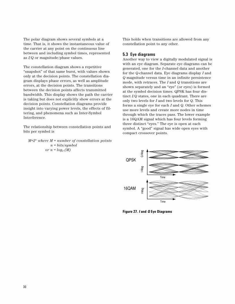
5.3 Eye diagramsAnother way to view a digitally modulated signal iswith an eye diagram. Separate eye diagrams can begenerated, one for the I-channel data and anotherfor the Q-channel data. Eye diagrams display I andQ magnitude versus time in an infinite persistencemode, with retraces. The I and Q transitions areshown separately and an “eye” (or eyes) is formedat the symbol decision times. QPSK has four dis-tinct I/Q states, one in each quadrant. There areonly two levels for I and two levels for Q. Thisforms a single eye for each I and Q. Other schemesuse more levels and create more nodes in timethrough which the traces pass. The lower exampleis a 16QAM signal which has four levels formingthree distinct “eyes.” The eye is open at each symbol. A “good” signal has wide open eyes with compact crossover points.

I-Mag

Q

-Mag

Time

QPSK

16QAM

I-Mag

Time

Figure 27. I and Q Eye Diagrams

31

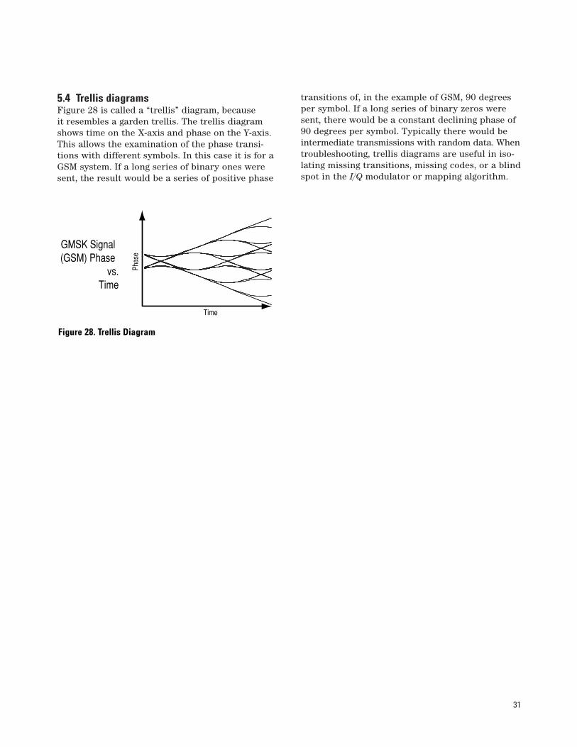
5.4 Trellis diagramsFigure 28 is called a “trellis” diagram, because it resembles a garden trellis. The trellis diagramshows time on the X-axis and phase on the Y-axis.This allows the examination of the phase transi-tions with different symbols. In this case it is for aGSM system. If a long series of binary ones weresent, the result would be a series of positive phase

transitions of, in the example of GSM, 90 degreesper symbol. If a long series of binary zeros weresent, there would be a constant declining phase of90 degrees per symbol. Typically there would beintermediate transmissions with random data. Whentroubleshooting, trellis diagrams are useful in iso-lating missing transitions, missing codes, or a blindspot in the I/Q modulator or mapping algorithm.

Phas

e

Time

GMSK Signal(GSM) Phase

vs.Time

Figure 28. Trellis Diagram

32

The RF spectrum is a finite resource and is sharedbetween users using multiplexing (sometimescalled channelization). Multiplexing is used to separate different users of the spectrum. This sec-tion covers multiplexing frequency, time, code, andgeography. Most communications systems use acombination of these multiplexing methods.

6.1 Multiplexing—frequencyFrequency Division Multiple Access (FDMA) splitsthe available frequency band into smaller fixed fre-quency channels. Each transmitter or receiver usesa separate frequency. This technique has been usedsince around 1900 and is still in use today. Trans-mitters are narrowband or frequency-limited. Anarrowband transmitter is used along with a receiverthat has a narrowband filter so that it can demodu-late the desired signal and reject unwanted signals,such as interfering signals from adjacent radios.

6.2 Multiplexing—timeTime-division multiplexing involves separating thetransmitters in time so that they can share thesame frequency. The simplest type is Time DivisionDuplex (TDD). This multiplexes the transmitterand receiver on the same frequency. TDD is used,for example, in a simple two-way radio where abutton is pressed to talk and released to listen.This kind of time division duplex, however, is veryslow. Modern digital radios like CT2 and DECT useTime Division Duplex but they multiplex hundredsof times per second. TDMA (Time Division Multi-ple Access) multiplexes several transmitters orreceivers on the same frequency. TDMA is used inthe GSM digital cellular system and also in the USNADC-TDMA system.

NarrowbandTransmitter

NarrowbandReceiver

TDMA Time Division Multiple-Access1

2

3

TDD Time Division Duplex

Am

plitu

de

Time

T R T R

A A A

B B BC C C

A B C

Figure 29. Multiplexing—Frequency Figure 30. Multiplexing—Time

6. Sharing the Channel

33

6.3 Multiplexing—codeCDMA is an access method where multiple usersare permitted to transmit simultaneously on thesame frequency. Frequency division multiplexing is still performed but the channel is 1.23 MHzwide. In the case of US CDMA telephones, an addi-tional type of channelization is added, in the formof coding.

In CDMA systems, users timeshare a higher-ratedigital channel by overlaying a higher-rate digitalsequence on their transmission. A differentsequence is assigned to each terminal so that thesignals can be discerned from one another by correlating them with the overlaid sequence. Thisis based on codes that are shared between the

base and mobile stations. Because of the choice of coding used, there is a limit of 64 code channels onthe forward link. The reverse link has no practicallimit to the number of codes available.

6.4 Multiplexing—geographyAnother kind of multiplexing is geographical orcellular. If two transmitter/receiver pairs are farenough apart, they can operate on the same fre-quency and not interfere with each other. Thereare only a few kinds of systems that do not usesome sort of geographic multiplexing. Clear-channelinternational broadcast stations, amateur stations,and some military low frequency radios are aboutthe only systems that have no geographic bound-aries and they broadcast around the world.

˜̃ Frequency

Amplitude

Time

F1

12

34

12

34

F1'

Figure 31. Multiplexing—Code

Figure 32. Multiplexing—Geography

34

6.5 Combining multiplexing modesIn most of these common communications sys-tems, different forms of multiplexing are generallycombined. For example, GSM uses FDMA, TDMA,FDD, and geographic. DECT uses FDMA, TDD, andgeographic multiplexing. For a full listing see thetable in section ten.

6.6 Penetration versus efficiencyPenetration means the ability of a signal to be used in environments where there is a lot of atten-uation, noise, or interference. One very commonexample is the use of pagers versus cellularphones. In many cases, pagers can receive signalseven if the user is inside a metal building or asteel-reinforced concrete structure like a modernskyscraper. Most pagers use a two-level FSK signalwhere the frequency deviation is large and themodulation rate (symbol rate) is quite slow. Thismakes it easy for the receiver to detect and demod-ulate the signal since the frequency difference islarge (the symbol locations are widely separated)and these different frequencies persist for a longtime (a slow symbol rate).

However, the factors causing good pager signalpenetration also cause inefficient informationtransmission. There are typically only two symbollocations. They are widely separated (approximately8 kHz), and a small number of symbols (500 to1200) are sent each second. Compare this with acellular system such as GSM which sends 270,833symbols each second. This is not a big problem forthe pager since all it needs to receive is its uniqueaddress and perhaps a short ASCII text message.

A cellular phone signal, however, must transmitlive duplex voice. This requires a much higher bitrate and a much more efficient modulation tech-nique. Cellular phones use more complex modula-tion formats (such as π/4 DQPSK and 0.3 GMSK)and faster symbol rates. Unfortunately, this greatlyreduces penetration and one way to compensate isto use more power. More power brings in a host ofother problems, as described previously.

35

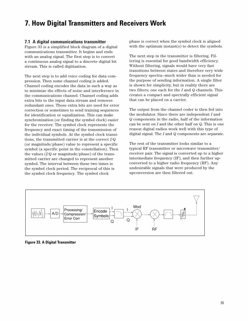
7.1 A digital communications transmitterFigure 33 is a simplified block diagram of a digital communications transmitter. It begins and endswith an analog signal. The first step is to convert a continuous analog signal to a discrete digital bitstream. This is called digitization.

The next step is to add voice coding for data com-pression. Then some channel coding is added.Channel coding encodes the data in such a way asto minimize the effects of noise and interference inthe communications channel. Channel coding addsextra bits to the input data stream and removesredundant ones. Those extra bits are used for errorcorrection or sometimes to send training sequencesfor identification or equalization. This can makesynchronization (or finding the symbol clock) easierfor the receiver. The symbol clock represents thefrequency and exact timing of the transmission ofthe individual symbols. At the symbol clock transi-tions, the transmitted carrier is at the correct I/Q(or magnitude/phase) value to represent a specificsymbol (a specific point in the constellation). Thenthe values (I/Q or magnitude/phase) of the trans-mitted carrier are changed to represent anothersymbol. The interval between these two times isthe symbol clock period. The reciprocal of this isthe symbol clock frequency. The symbol clock

phase is correct when the symbol clock is alignedwith the optimum instant(s) to detect the symbols.

The next step in the transmitter is filtering. Fil-tering is essential for good bandwidth efficiency.Without filtering, signals would have very fast transitions between states and therefore very widefrequency spectra—much wider than is needed forthe purpose of sending information. A single filteris shown for simplicity, but in reality there are two filters; one each for the I and Q channels. This creates a compact and spectrally efficient signalthat can be placed on a carrier.

The output from the channel coder is then fed intothe modulator. Since there are independent I andQ components in the radio, half of the informationcan be sent on I and the other half on Q. This is onereason digital radios work well with this type ofdigital signal. The I and Q components are separate.

The rest of the transmitter looks similar to a typical RF transmitter or microwave transmitter/receiver pair. The signal is converted up to a higherintermediate frequency (IF), and then further up-converted to a higher radio frequency (RF). Anyundesirable signals that were produced by theupconversion are then filtered out.

A/D

ModI I

Q Q

IF RF

Processing/Compression/Error Corr

EncodeSymbols

Figure 33. A Digital Transmitter

7. How Digital Transmitters and Receivers Work

36

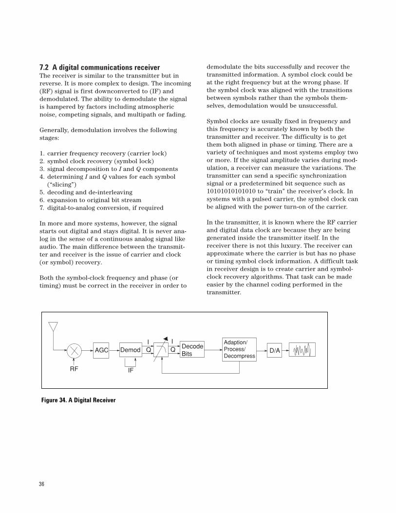
7.2 A digital communications receiverThe receiver is similar to the transmitter but inreverse. It is more complex to design. The incoming(RF) signal is first downconverted to (IF) anddemodulated. The ability to demodulate the signalis hampered by factors including atmosphericnoise, competing signals, and multipath or fading.

Generally, demodulation involves the followingstages:

1. carrier frequency recovery (carrier lock)2. symbol clock recovery (symbol lock)3. signal decomposition to I and Q components4. determining I and Q values for each symbol

(“slicing”)5. decoding and de-interleaving6. expansion to original bit stream7. digital-to-analog conversion, if required

In more and more systems, however, the signalstarts out digital and stays digital. It is never ana-log in the sense of a continuous analog signal likeaudio. The main difference between the transmit-ter and receiver is the issue of carrier and clock(or symbol) recovery.

Both the symbol-clock frequency and phase (ortiming) must be correct in the receiver in order to

demodulate the bits successfully and recover thetransmitted information. A symbol clock could beat the right frequency but at the wrong phase. Ifthe symbol clock was aligned with the transitionsbetween symbols rather than the symbols them-selves, demodulation would be unsuccessful.

Symbol clocks are usually fixed in frequency andthis frequency is accurately known by both thetransmitter and receiver. The difficulty is to getthem both aligned in phase or timing. There are avariety of techniques and most systems employ twoor more. If the signal amplitude varies during mod-ulation, a receiver can measure the variations. Thetransmitter can send a specific synchronizationsignal or a predetermined bit sequence such as10101010101010 to “train” the receiver’s clock. Insystems with a pulsed carrier, the symbol clock canbe aligned with the power turn-on of the carrier.

In the transmitter, it is known where the RF carrierand digital data clock are because they are beinggenerated inside the transmitter itself. In thereceiver there is not this luxury. The receiver canapproximate where the carrier is but has no phaseor timing symbol clock information. A difficult taskin receiver design is to create carrier and symbol-clock recovery algorithms. That task can be madeeasier by the channel coding performed in thetransmitter.

AGC Demod QI I

QAdaption/Process/Decompress

D/A

IFRF

DecodeBits

Figure 34. A Digital Receiver

37

Complex tradeoffs in frequency, phase, timing, and modulation are made for interference-free,multiple-user communications systems. It is neces-sary to accurately measure parameters in digitalRF communications systems to make the righttradeoffs. Measurements include analyzing the mod-ulator and demodulator, characterizing the trans-mitted signal quality, locating causes of high Bit-Error-Rate, and investigating new modulationtypes. Measurements on digital RF communicationssystems generally fall into four categories: power,frequency, timing, and modulation accuracy.

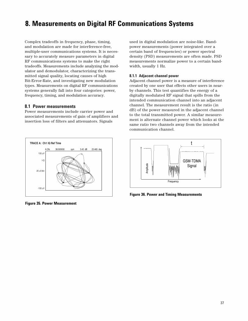
8.1 Power measurementsPower measurements include carrier power andassociated measurements of gain of amplifiers andinsertion loss of filters and attenuators. Signals

used in digital modulation are noise-like. Band-power measurements (power integrated over a certain band of frequencies) or power spectral density (PSD) measurements are often made. PSDmeasurements normalize power to a certain band-width, usually 1 Hz.

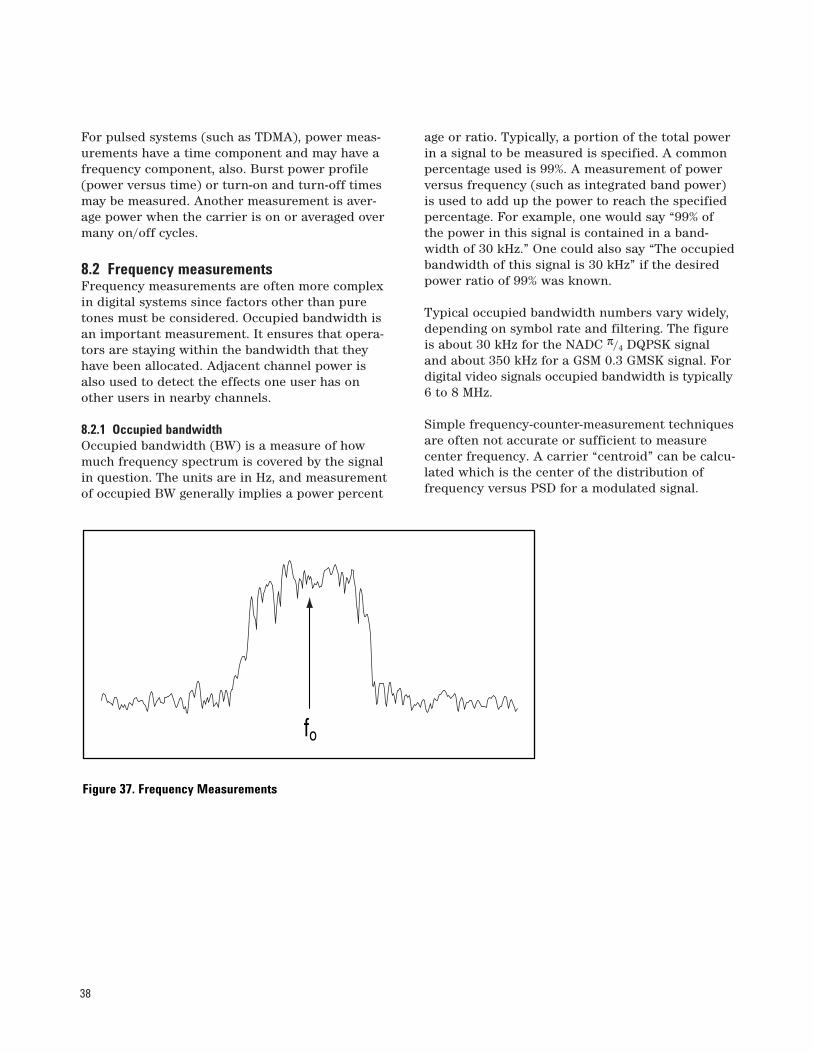
8.1.1 Adjacent channel powerAdjacent channel power is a measure of interferencecreated by one user that effects other users in near-by channels. This test quantifies the energy of adigitally modulated RF signal that spills from theintended communication channel into an adjacentchannel. The measurement result is the ratio (indB) of the power measured in the adjacent channelto the total transmitted power. A similar measure-ment is alternate channel power which looks at thesame ratio two channels away from the intendedcommunication channel.

TRACE A: Ch1 IQ Ref Time

A Ofs 38.500000 sym 3.43 dB 23.465 deg

100 uV

I-Q

20 uV/div

-100 uV

Ampl

itude

Frequency

GSM-TDMASignal

t

Figure 35. Power Measurement

Figure 36. Power and Timing Measurements

8. Measurements on Digital RF Communications Systems

38

For pulsed systems (such as TDMA), power meas-urements have a time component and may have afrequency component, also. Burst power profile(power versus time) or turn-on and turn-off timesmay be measured. Another measurement is aver-age power when the carrier is on or averaged overmany on/off cycles.

8.2 Frequency measurementsFrequency measurements are often more complexin digital systems since factors other than puretones must be considered. Occupied bandwidth isan important measurement. It ensures that opera-tors are staying within the bandwidth that theyhave been allocated. Adjacent channel power isalso used to detect the effects one user has onother users in nearby channels.

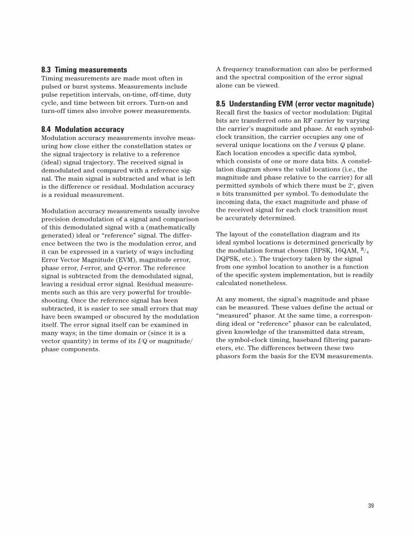
8.2.1 Occupied bandwidthOccupied bandwidth (BW) is a measure of howmuch frequency spectrum is covered by the signalin question. The units are in Hz, and measurementof occupied BW generally implies a power percent

age or ratio. Typically, a portion of the total powerin a signal to be measured is specified. A commonpercentage used is 99%. A measurement of powerversus frequency (such as integrated band power)is used to add up the power to reach the specifiedpercentage. For example, one would say “99% ofthe power in this signal is contained in a band-width of 30 kHz.” One could also say “The occupiedbandwidth of this signal is 30 kHz” if the desiredpower ratio of 99% was known.

Typical occupied bandwidth numbers vary widely,depending on symbol rate and filtering. The figureis about 30 kHz for the NADC π/4 DQPSK signaland about 350 kHz for a GSM 0.3 GMSK signal. Fordigital video signals occupied bandwidth is typically6 to 8 MHz.

Simple frequency-counter-measurement techniquesare often not accurate or sufficient to measurecenter frequency. A carrier “centroid” can be calcu-lated which is the center of the distribution of frequency versus PSD for a modulated signal.

fo

Figure 37. Frequency Measurements

39

8.3 Timing measurementsTiming measurements are made most often inpulsed or burst systems. Measurements includepulse repetition intervals, on-time, off-time, dutycycle, and time between bit errors. Turn-on andturn-off times also involve power measurements.

8.4 Modulation accuracyModulation accuracy measurements involve meas-uring how close either the constellation states orthe signal trajectory is relative to a reference(ideal) signal trajectory. The received signal isdemodulated and compared with a reference sig-nal. The main signal is subtracted and what is leftis the difference or residual. Modulation accuracyis a residual measurement.

Modulation accuracy measurements usually involveprecision demodulation of a signal and comparisonof this demodulated signal with a (mathematicallygenerated) ideal or “reference” signal. The differ-ence between the two is the modulation error, andit can be expressed in a variety of ways includingError Vector Magnitude (EVM), magnitude error,phase error, I-error, and Q-error. The reference signal is subtracted from the demodulated signal,leaving a residual error signal. Residual measure-ments such as this are very powerful for trouble-shooting. Once the reference signal has been subtracted, it is easier to see small errors that mayhave been swamped or obscured by the modulationitself. The error signal itself can be examined inmany ways; in the time domain or (since it is a vector quantity) in terms of its I/Q or magnitude/phase components.

A frequency transformation can also be performedand the spectral composition of the error signalalone can be viewed.

8.5 Understanding EVM (error vector magnitude)Recall first the basics of vector modulation: Digitalbits are transferred onto an RF carrier by varyingthe carrier’s magnitude and phase. At each symbol-clock transition, the carrier occupies any one ofseveral unique locations on the I versus Q plane.Each location encodes a specific data symbol,which consists of one or more data bits. A constel-lation diagram shows the valid locations (i.e., themagnitude and phase relative to the carrier) for allpermitted symbols of which there must be 2n, givenn bits transmitted per symbol. To demodulate theincoming data, the exact magnitude and phase ofthe received signal for each clock transition mustbe accurately determined.

The layout of the constellation diagram and itsideal symbol locations is determined generically bythe modulation format chosen (BPSK, 16QAM, π/4

DQPSK, etc.). The trajectory taken by the signalfrom one symbol location to another is a functionof the specific system implementation, but is readilycalculated nonetheless.

At any moment, the signal’s magnitude and phasecan be measured. These values define the actual or“measured” phasor. At the same time, a correspon-ding ideal or “reference” phasor can be calculated,given knowledge of the transmitted data stream,the symbol-clock timing, baseband filtering param-eters, etc. The differences between these two phasors form the basis for the EVM measurements.

40

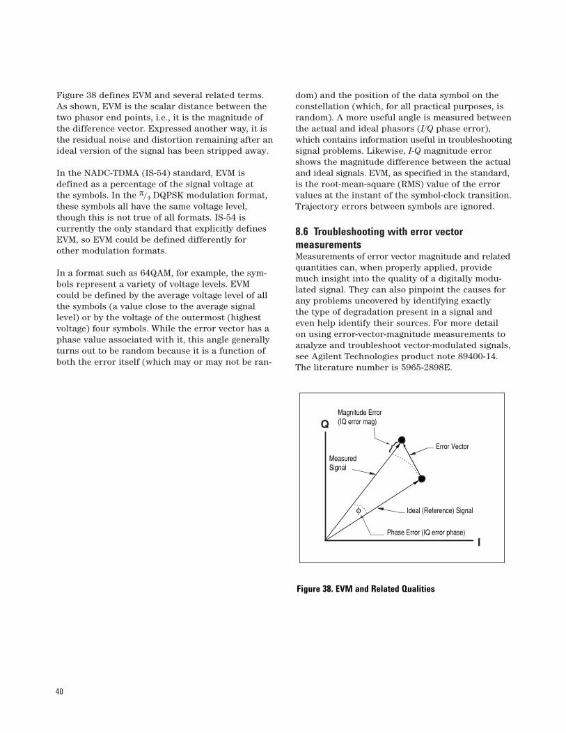
Figure 38 defines EVM and several related terms.As shown, EVM is the scalar distance between thetwo phasor end points, i.e., it is the magnitude ofthe difference vector. Expressed another way, it isthe residual noise and distortion remaining after anideal version of the signal has been stripped away.

In the NADC-TDMA (IS-54) standard, EVM isdefined as a percentage of the signal voltage at the symbols. In the π/4 DQPSK modulation format,these symbols all have the same voltage level,though this is not true of all formats. IS-54 is currently the only standard that explicitly definesEVM, so EVM could be defined differently for other modulation formats.

In a format such as 64QAM, for example, the sym-bols represent a variety of voltage levels. EVMcould be defined by the average voltage level of allthe symbols (a value close to the average signallevel) or by the voltage of the outermost (highestvoltage) four symbols. While the error vector has aphase value associated with it, this angle generallyturns out to be random because it is a function ofboth the error itself (which may or may not be ran-

dom) and the position of the data symbol on theconstellation (which, for all practical purposes, israndom). A more useful angle is measured betweenthe actual and ideal phasors (I/Q phase error),which contains information useful in troubleshootingsignal problems. Likewise, I-Q magnitude errorshows the magnitude difference between the actualand ideal signals. EVM, as specified in the standard,is the root-mean-square (RMS) value of the errorvalues at the instant of the symbol-clock transition.Trajectory errors between symbols are ignored.

8.6 Troubleshooting with error vector measurementsMeasurements of error vector magnitude and relatedquantities can, when properly applied, providemuch insight into the quality of a digitally modu-lated signal. They can also pinpoint the causes forany problems uncovered by identifying exactly the type of degradation present in a signal andeven help identify their sources. For more detail on using error-vector-magnitude measurements toanalyze and troubleshoot vector-modulated signals,see Agilent Technologies product note 89400-14.The literature number is 5965-2898E.

{

I

QMagnitude Error (IQ error mag)

Error Vector

Ideal (Reference) Signal

Phase Error (IQ error phase)

MeasuredSignal

φ

Figure 38. EVM and Related Qualities

41

EVM measurements are growing rapidly in accept-ance, having already been written into such impor-tant system standards as NADC and PHS, and theyare poised to appear in several upcoming standardsincluding those for digital video transmission.

8.7 Magnitude versus phase errorDifferent error mechanisms affect signals in differ-ent ways: in magnitude only, phase only, or bothsimultaneously. Knowing the relative amounts ofeach type of error can quickly confirm or rule outcertain types of problems. Thus, the first diagnos-tic step is to resolve EVM into its magnitude andphase error components (see Figure 38) and com-pare their relative sizes.

When the average phase error (in degrees) is sub-stantially larger than the average magnitude error

(in percent), some sort of unwanted phase modula-tion is the dominant error mode. This could becaused by noise, spurious or cross-coupling problemsin the frequency reference, phase-locked loops, orother frequency-generating stages. Residual AM isevidenced by magnitude errors that are significantlylarger than the phase angle errors.

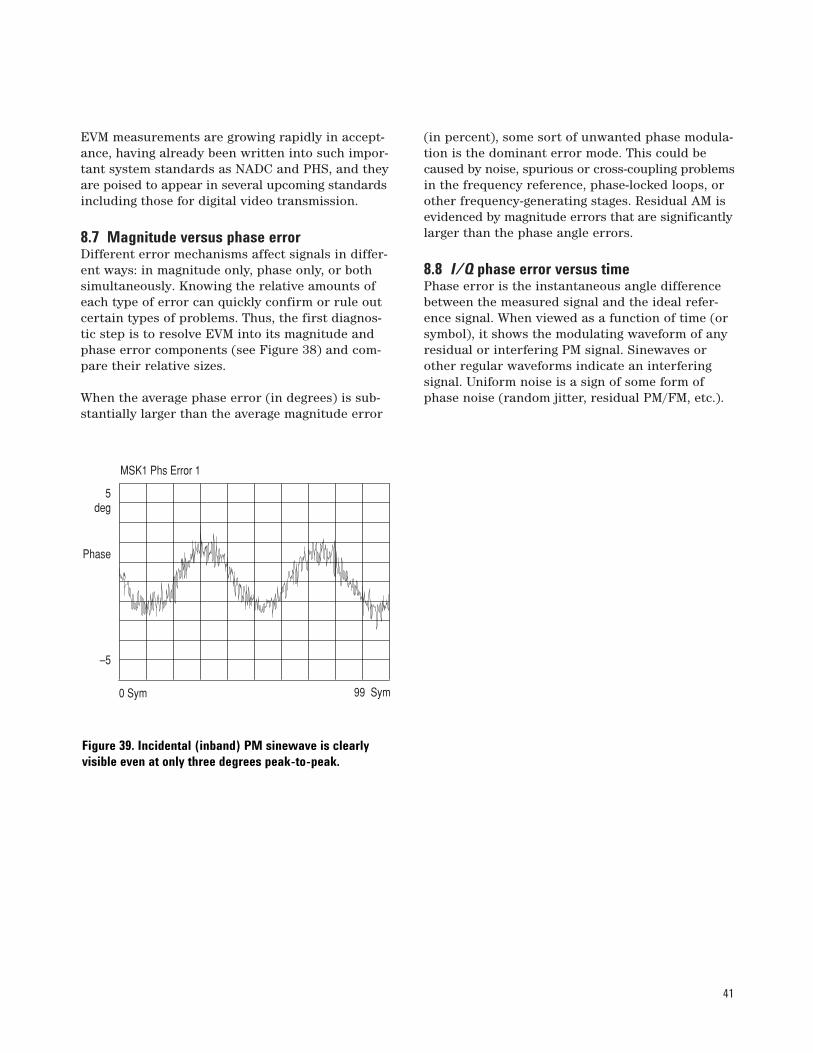
8.8 I/Q phase error versus timePhase error is the instantaneous angle differencebetween the measured signal and the ideal refer-ence signal. When viewed as a function of time (orsymbol), it shows the modulating waveform of anyresidual or interfering PM signal. Sinewaves orother regular waveforms indicate an interferingsignal. Uniform noise is a sign of some form ofphase noise (random jitter, residual PM/FM, etc.).

5deg

Phase

–5

99 Sym 0 Sym

MSK1 Phs Error 1

Figure 39. Incidental (inband) PM sinewave is clearly visible even at only three degrees peak-to-peak.

42

A perfect signal will have a uniform constellationthat is perfectly symmetric about the origin. I/Qimbalance is indicated when the constellation isnot “square,” i.e., when the Q-axis height does notequal the I-axis width. Quadrature error is seen inany “tilt” to the constellation. Quadrature error iscaused when the phase relationship between the I and Q vectors is not exactly 90 degrees.

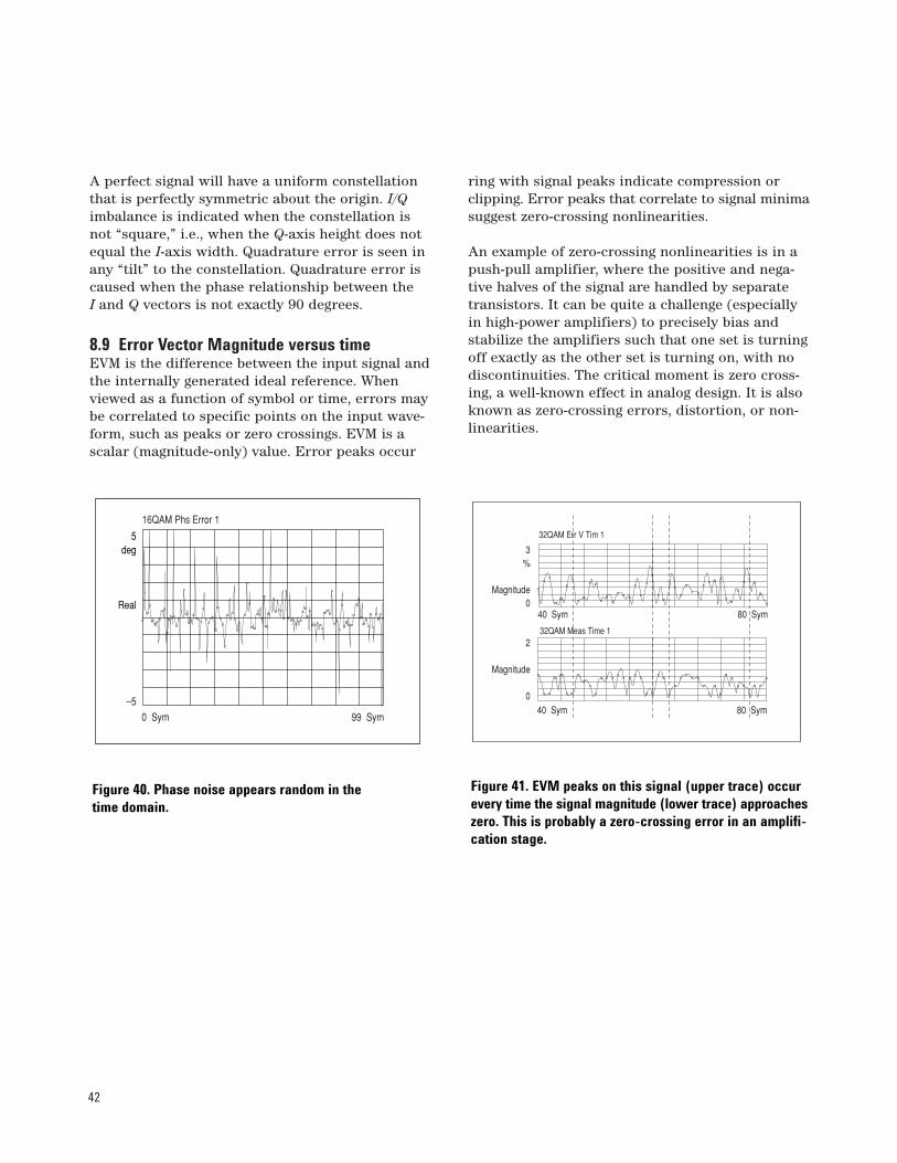
8.9 Error Vector Magnitude versus time EVM is the difference between the input signal andthe internally generated ideal reference. Whenviewed as a function of symbol or time, errors maybe correlated to specific points on the input wave-form, such as peaks or zero crossings. EVM is ascalar (magnitude-only) value. Error peaks occur

ring with signal peaks indicate compression orclipping. Error peaks that correlate to signal minimasuggest zero-crossing nonlinearities.

An example of zero-crossing nonlinearities is in apush-pull amplifier, where the positive and nega-tive halves of the signal are handled by separatetransistors. It can be quite a challenge (especiallyin high-power amplifiers) to precisely bias and stabilize the amplifiers such that one set is turningoff exactly as the other set is turning on, with nodiscontinuities. The critical moment is zero cross-ing, a well-known effect in analog design. It is alsoknown as zero-crossing errors, distortion, or non-linearities.

5deg

Real

–5

0 Sym 99 Sym

16QAM Phs Error 1

3%

Magnitude0

2

Magnitude

0

32QAM Err V Tim 1

40 Sym 80 Sym

32QAM Meas Time 1

40 Sym 80 Sym

Figure 40. Phase noise appears random in the time domain.

Figure 41. EVM peaks on this signal (upper trace) occurevery time the signal magnitude (lower trace) approacheszero. This is probably a zero-crossing error in an amplifi-cation stage.

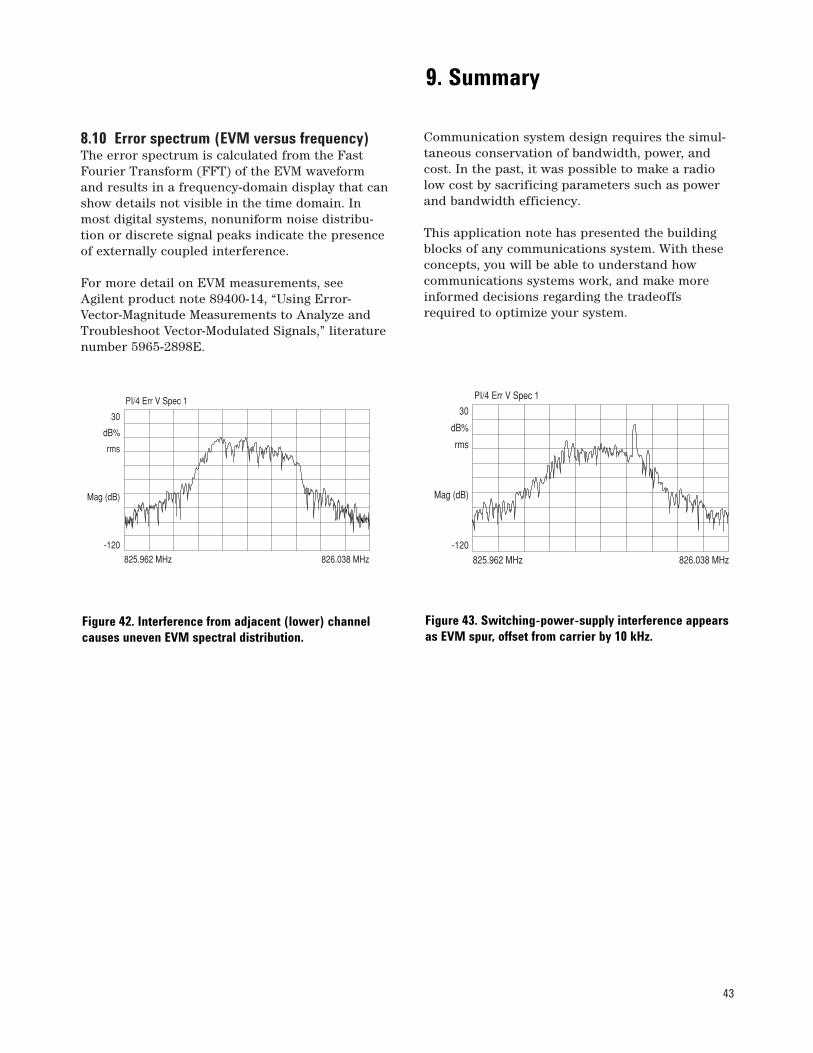
43

8.10 Error spectrum (EVM versus frequency)The error spectrum is calculated from the FastFourier Transform (FFT) of the EVM waveform and results in a frequency-domain display that canshow details not visible in the time domain. Inmost digital systems, nonuniform noise distribu-tion or discrete signal peaks indicate the presenceof externally coupled interference.

For more detail on EVM measurements, see Agilent product note 89400-14, “Using Error-Vector-Magnitude Measurements to Analyze andTroubleshoot Vector-Modulated Signals,” literaturenumber 5965-2898E.

Communication system design requires the simul-taneous conservation of bandwidth, power, andcost. In the past, it was possible to make a radiolow cost by sacrificing parameters such as powerand bandwidth efficiency.

This application note has presented the buildingblocks of any communications system. With theseconcepts, you will be able to understand how communications systems work, and make moreinformed decisions regarding the tradeoffsrequired to optimize your system.

30

dB%

rms

Mag (dB)

-120

825.962 MHz 826.038 MHz

PI/4 Err V Spec 130

dB%

rms

Mag (dB)

-120

825.962 MHz 826.038 MHz

PI/4 Err V Spec 1

Figure 42. Interference from adjacent (lower) channelcauses uneven EVM spectral distribution.

Figure 43. Switching-power-supply interference appearsas EVM spur, offset from carrier by 10 kHz.

9. Summary

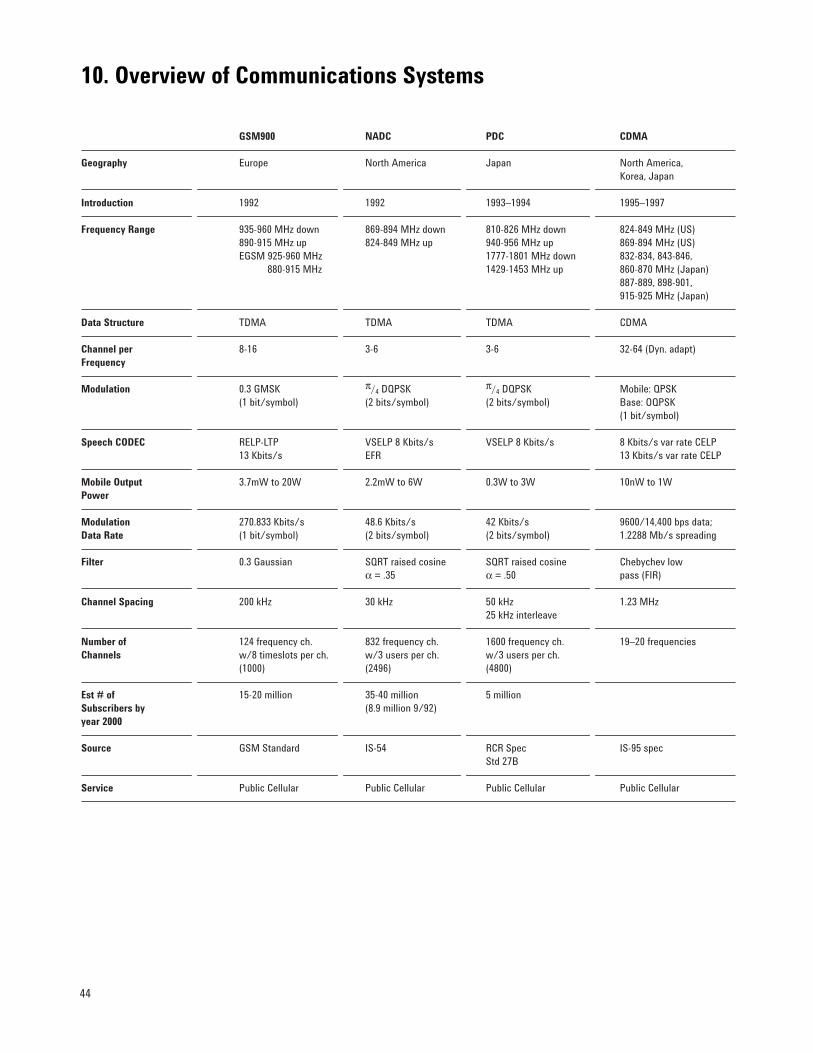
44

GSM900 NADC PDC CDMA

Geography Europe North America Japan North America,Korea, Japan

Introduction 1992 1992 1993–1994 1995–1997

Frequency Range 935-960 MHz down 869-894 MHz down 810-826 MHz down 824-849 MHz (US) 890-915 MHz up 824-849 MHz up 940-956 MHz up 869-894 MHz (US) EGSM 925-960 MHz 1777-1801 MHz down 832-834, 843-846,

880-915 MHz 1429-1453 MHz up 860-870 MHz (Japan) 887-889, 898-901, 915-925 MHz (Japan)

Data Structure TDMA TDMA TDMA CDMA

Channel per 8-16 3-6 3-6 32-64 (Dyn. adapt) Frequency

Modulation 0.3 GMSK π/4 DQPSK π/4 DQPSK Mobile: QPSK(1 bit/symbol) (2 bits/symbol) (2 bits/symbol) Base: OQPSK

(1 bit/symbol)

Speech CODEC RELP-LTP VSELP 8 Kbits/s VSELP 8 Kbits/s 8 Kbits/s var rate CELP 13 Kbits/s EFR 13 Kbits/s var rate CELP

Mobile Output 3.7mW to 20W 2.2mW to 6W 0.3W to 3W 10nW to 1W Power

Modulation 270.833 Kbits/s 48.6 Kbits/s 42 Kbits/s 9600/14,400 bps data; Data Rate (1 bit/symbol) (2 bits/symbol) (2 bits/symbol) 1.2288 Mb/s spreading

Filter 0.3 Gaussian SQRT raised cosine SQRT raised cosine Chebychev low α = .35 α = .50 pass (FIR)

Channel Spacing 200 kHz 30 kHz 50 kHz 1.23 MHz 25 kHz interleave

Number of 124 frequency ch. 832 frequency ch. 1600 frequency ch. 19–20 frequencies Channels w/8 timeslots per ch. w/3 users per ch. w/3 users per ch.

(1000) (2496) (4800)

Est # of 15-20 million 35-40 million 5 million Subscribers by (8.9 million 9/92) year 2000

Source GSM Standard IS-54 RCR Spec IS-95 specStd 27B

Service Public Cellular Public Cellular Public Cellular Public Cellular

10. Overview of Communications Systems

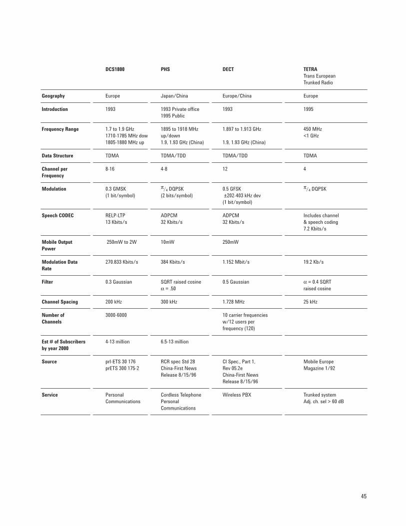
45

DCS1800 PHS DECT TETRATrans European Trunked Radio

Geography Europe Japan/China Europe/China Europe

Introduction 1993 1993 Private office 1993 19951995 Public

Frequency Range 1.7 to 1.9 GHz 1895 to 1918 MHz 1.897 to 1.913 GHz 450 MHz 1710-1785 MHz down up/down <1 GHz1805-1880 MHz up 1.9, 1.93 GHz (China) 1.9, 1.93 GHz (China)

Data Structure TDMA TDMA/TDD TDMA/TDD TDMA

Channel per 8-16 4-8 12 4 Frequency

Modulation 0.3 GMSK π/4 DQPSK 0.5 GFSK π/4 DQPSK(1 bit/symbol) (2 bits/symbol) ±202-403 kHz dev

(1 bit/symbol)

Speech CODEC RELP-LTP ADPCM ADPCM Includes channel 13 Kbits/s 32 Kbits/s 32 Kbits/s & speech coding

7.2 Kbits/s

Mobile Output 250mW to 2W 10mW 250mWPower

Modulation Data 270.833 Kbits/s 384 Kbits/s 1.152 Mbit/s 19.2 Kb/s Rate

Filter 0.3 Gaussian SQRT raised cosine 0.5 Gaussian α = 0.4 SQRT α = .50 raised cosine

Channel Spacing 200 kHz 300 kHz 1.728 MHz 25 kHz

Number of 3000-6000 10 carrier frequencies Channels w/12 users per

frequency (120)

Est # of Subscribers 4-13 million 6.5-13 million by year 2000

Source prI-ETS 30 176 RCR spec Std 28 CI Spec., Part 1, Mobile Europe prETS 300 175-2 China-First News Rev 05.2e Magazine 1/92

Release 8/15/96 China-First News Release 8/15/96

Service Personal Cordless Telephone Wireless PBX Trunked system Communications Personal Adj. ch. sel > 60 dB

Communications

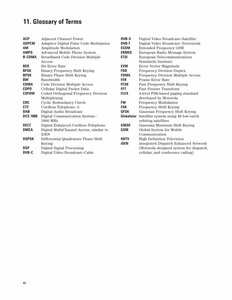
46

ACP Adjacent Channel PowerADPCM Adaptive Digital Pulse Code ModulationAM Amplitude ModulationAMPS Advanced Mobile Phone SystemB-CDMA Broadband Code Division Multiple

AccessBER Bit Error RateBFSK Binary Frequency Shift KeyingBPSK Binary Phase Shift KeyingBW BandwidthCDMA Code Division Multiple AccessCDPD Cellular Digital Packet DataCOFDM Coded Orthogonal Frequency Division

MultiplexingCRC Cyclic Redundancy CheckCT2 Cordless Telephone—2DAB Digital Audio BroadcastDCS 1800 Digital Communication System—

1800 MHzDECT Digital Enhanced Cordless TelephoneDMCA Digital MultiChannel Access, similar to

iDENDQPSK Differential Quadrature Phase Shift

KeyingDSP Digital Signal ProcessingDVB-C Digital Video Broadcast—Cable

DVB-S Digital Video Broadcast—SatelliteDVB-T Digital Video Broadcast—TerrestrialEGSM Extended Frequency GSMERMES European Radio Message SystemETSI European Telecommunications

Standards InstituteEVM Error Vector MagnitudeFDD Frequency Division DuplexFDMA Frequency Division Multiple AccessFER Frame Error RateFFSK Fast Frequency Shift KeyingFFT Fast Fourier TransformFLEX 4-level FSK-based paging standard

developed by MotorolaFM Frequency ModulationFSK Frequency Shift KeyingGFSK Gaussian Frequency Shift Keying Globalstar Satellite system using 48 low-earth

orbiting satellitesGMSK Gaussian Minimum Shift KeyingGSM Global System for Mobile

CommunicationHDTV High Definition TelevisioniDEN integrated Dispatch Enhanced Network

(Motorola designed system for dispatch, cellular, and conference calling)

11. Glossary of Terms

47

IF Intermediate FrequencyI/Q In phase/QuadratureIridium Motorola voice/data 66-satellite system

worldwideISI Intersymbol InterferenceIS-54 Interim Standard for US Digital Cellular

(NADC)IS-95 Interim Standard for US Code Division

Multiple AccessIS-136 Interim Standard for NADC with Digital

Control ChannelsLMDS Local Multipoint Distribution SystemMFSK Minimum Frequency Shift KeyingMMDS Multichannel Multipoint Distribution

SystemMPSK Minimum Phase Shift KeyingMSK Minimum Shift KeyingNADC North American Digital Cellular systemOFDM Orthogonal Frequency Division

MultiplexingOQPSK Offset Quadrature Phase Shift KeyingPACS Personal Access Communications

Service

PCS Personal Communications SystemPCM Pulse Code ModulationPDC Pacific Digital Cellular System

(formerly JDC)PHS Personal Handyphone System

(formerly PHP)PRBS Pseudo-Random Bit SequencePSD Power Spectral DensityPSK Phase Shift KeyingQAM Quadrature Amplitude ModulationQPSK Quadrature Phase Shift KeyingRAM Wireless data networkRF Radio FrequencyRMS Root Mean SquareSQRT Square RootTDD Time Division DuplexTDMA Time Division Multiple AccessTETRA Trans European Trunked RadioTFTS Terrestrial Flight Telephone SystemVSB Vestigal Side BandWLL Wireless Local Loop

By internet, phone, or fax, get assistance with all your test and measurement needs.

Online Assistancewww.agilent.com/find/assistPhone or FaxUnited States:(tel) 1 800 452 4844

Canada:(tel) 1 877 894 4414(fax) (905) 206 4120

Europe:(tel) (31 20) 547 2323(fax) (31 20) 547 2390

Japan:(tel) (81) 426 56 7832(fax) (81) 426 56 7840

Latin America:(tel) (305) 269 7500(fax) (305) 269 7599

Australia:(tel) 1 800 629 485 (fax) (61 3) 9272 0749

New Zealand:(tel) 0 800 738 378 (fax) (64 4) 495 8950

Asia Pacific:(tel) (852) 3197 7777(fax) (852) 2506 9284

Product specifications and descriptions in this document subject to change without notice.

Copyright © 2001 Agilent TechnologiesPrinted in U.S.A. March 14, 20015965-7160E