feature based modulation recognition for intrapulse...
TRANSCRIPT
FEATURE BASED MODULATION RECOGNITION FOR INTRAPULSE MODULATIONS
A THESIS SUBMITTED TO THE GRADUATE SCHOOL OF NATURAL AND APPLIED SCIENCES
OF MIDDLE EAST TECHNICAL UNIVERSITY
BY
GÖZDE ÇEVİK
IN PARTIAL FULFILLMENT OF THE REQUIREMENTS FOR
THE DEGREE OF MASTER OF SCIENCE IN
ELECTRICAL AND ELECTRONICS ENGINEERING
SEPTEMBER 2006
Approval of the Graduate School of Natural and Applied Sciences
Prof. Dr. Canan Özgen
Director
I certify that this thesis satisfies all the requirements as a thesis for the degree of Master of
Science
Prof. Dr. İsmet Erkmen
Head of Department
This is to certify that we have read this thesis and that in our opinion it is fully adequate, in
scope and quality, as a thesis for the degree of Master of Science.
Assoc.Prof.Dr.Gözde Bozdağı Akar
Supervisor
Examining Committee Members
Assoc. Prof. Dr. Engin Tuncer (METU, EEE)
Assoc. Prof. Dr. Gözde Bozdağı Akar (METU, EEE)
Assist. Prof. Dr. Çağatay Candan (METU, EEE)
Assist. Prof. Dr. Özgür Yılmaz (METU, EEE)
Alaattin Dökmen (M. Sc.) (ASELSAN)

PLAGIARISM
I hereby declare that all information in this document has been obtained and presented in accordance with academic rules and ethical conduct. I also declare that, as required by these rules and conduct, I have fully cited and referenced all material and results that are not original to this work.
Name, Last name: Gözde ÇEVİK
Signature :
iii
ABSTRACT
FEATURE BASED MODULATION RECOGNITION
FOR INTRAPULSE MODULATIONS
Çevik, Gözde
M.S., Department of Electrical and Electronics Engineering
Supervisor : Assoc. Prof. Dr. Gözde Bozdağı Akar
September 2006, 143 pages
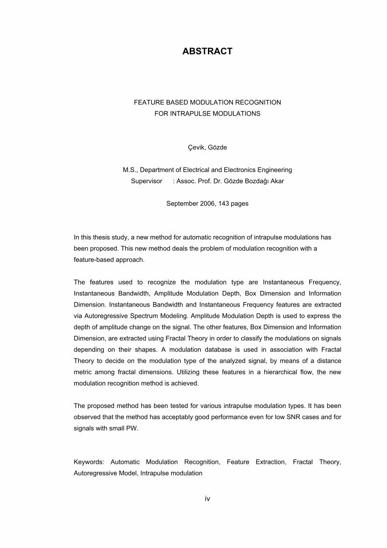
In this thesis study, a new method for automatic recognition of intrapulse modulations has
been proposed. This new method deals the problem of modulation recognition with a
feature-based approach.
The features used to recognize the modulation type are Instantaneous Frequency,
Instantaneous Bandwidth, Amplitude Modulation Depth, Box Dimension and Information
Dimension. Instantaneous Bandwidth and Instantaneous Frequency features are extracted
via Autoregressive Spectrum Modeling. Amplitude Modulation Depth is used to express the
depth of amplitude change on the signal. The other features, Box Dimension and Information
Dimension, are extracted using Fractal Theory in order to classify the modulations on signals
depending on their shapes. A modulation database is used in association with Fractal
Theory to decide on the modulation type of the analyzed signal, by means of a distance
metric among fractal dimensions. Utilizing these features in a hierarchical flow, the new
modulation recognition method is achieved.
The proposed method has been tested for various intrapulse modulation types. It has been
observed that the method has acceptably good performance even for low SNR cases and for
signals with small PW.
Keywords: Automatic Modulation Recognition, Feature Extraction, Fractal Theory,
Autoregressive Model, Intrapulse modulation
iv
ÖZ
DARBE İÇİ MODÜLASYONLARIN
ÖZNİTELİKLERE BAĞLI OLARAK TANIMLANMASI
Çevik, Gözde
Master, Elektrik ve Elektronik Mühendisliği Bölümü
Tez Yöneticisi : Doç. Dr. Gözde Bozdağı Akar
Eylül 2006, 143 sayfa
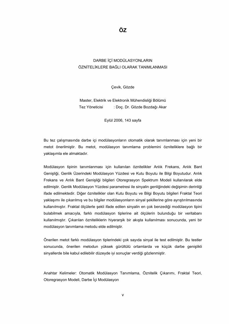
Bu tez çalışmasında darbe içi modülasyonların otomatik olarak tanımlanması için yeni bir
metot önerilmiştir. Bu metot, modülasyon tanımlama problemini özniteliklere bağlı bir
yaklaşımla ele almaktadır.
Modülasyon tipinin tanımlanması için kullanılan öznitelikler Anlık Frekans, Anlık Bant
Genişliği, Genlik Üzerindeki Modülasyon Yüzdesi ve Kutu Boyutu ile Bilgi Boyutudur. Anlık
Frekans ve Anlık Bant Genişliği bilgileri Otoregrasyon Spektrum Modeli kullanılarak elde
edilmiştir. Genlik Modülasyon Yüzdesi parametresi ile sinyalin genliğindeki değişimin derinliği
ifade edilmektedir. Diğer öznitelikler olan Kutu Boyutu ve Bilgi Boyutu bilgileri Fraktal Teori
yaklaşımı ile çıkarılmış ve bu bilgiler modülasyonların sinyal şekillerine göre ayrıştırılmasında
kullanılmıştır. Fraktal ölçülerle şekli ifade edilen sinyalin en çok benzediği modülasyon tipini
bulabilmek amacıyla, farklı modülasyon tiplerine ait ölçülerin bulunduğu bir veritabanı
kullanılmıştır. Çıkarılan özniteliklerin hiyerarşik bir akışta kullanılması sonucunda, yeni bir
modülasyon tanımlama metodu elde edilmiştir.
Önerilen metot farklı modülasyon tiplerindeki çok sayıda sinyal ile test edilmiştir. Bu testler
sonucunda, önerilen metodun yüksek gürültülü ortamlarda ve küçük darbe genişlikli
sinyallerde bile kabul edilebilir düzeyde iyi sonuçlar verdiği gözlenmiştir.
Anahtar Kelimeler: Otomatik Modülasyon Tanımlama, Öznitelik Çıkarımı, Fraktal Teori,
Otoregrasyon Modeli, Darbe İçi Modülasyon
v

To My Parents,
vi

ACKNOWLEDGEMENTS
I would like to express my deepest gratitude to my supervisor Assoc. Prof. Dr. Gözde
Bozdağı Akar for her guidance, advice, criticism, encouragements and insight throughout the
research. This thesis would not have been completed without her affinity and support.
I also want to thank ASELSAN Inc. for the facilities provided for the completion of this thesis.
Beyond my colleagues, technical assistance of Alaattin Dökmen and Öznur Ateş Yıldız are
also gratefully acknowledged.
I would like to thank my whole family; for their care on me from the beginning of my life, their
prayers, and their trust on me that I could accomplish this task.
Finally, I would especially like to thank my love, Kadir, for his emotional support,
comprehension, personal sacrifice and patience besides his technical support and guiding
suggestions. He was always there as my congenial companion anytime I lose my way.
vii
TABLE OF CONTENTS PLAGIARISM ........................................................................................................................... iii
ABSTRACT ..............................................................................................................................iv
ÖZ .........................................................................................................................................v
ACKNOWLEDGEMENTS ....................................................................................................... vii
TABLE OF CONTENTS......................................................................................................... viii
LIST OF TABLES......................................................................................................................x
LIST OF FIGURES................................................................................................................. xiii
LIST OF ABBREVIATIONS................................................................................................... xvii
CHAPTERS
1. INTRODUCTION.................................................................................................................. 1
1.1 BACKGROUND .......................................................................................................... 1
1.2 OUTLINE OF THESIS................................................................................................. 4
2. INTRAPULSE MODULATIONS ........................................................................................... 6
2.1. PURPOSE OF RADAR SYSTEMS FOR APPLYING MODULATIONS ON PULSE.. 6
2.2. INTRAPULSE MODULATIONS .................................................................................. 8
2.2.1. AMPLITUDE MODULATION ON PULSE............................................................. 8
2.2.2. FREQUENCY MODULATION ON PULSE........................................................... 9
2.2.3. PHASE MODULATION ON PULSE ..................................................................... 9
3. AUTOMATIC RECOGNITION OF INTRAPULSE MODULATIONS .................................. 12
4. FEATURE BASED MODULATION RECOGNITION ......................................................... 18
4.1 METHODOLOGY FOR FEATURE EXTRACTION................................................... 18
4.1.1. INSTANTANEOUS FREQUENCY AND BANDWIDTH...................................... 18
4.1.2. BOX DIMENSION AND INFORMATION DIMENSION ...................................... 20
4.1.3. PERCENT AM DEPTH....................................................................................... 25
4.2 PROPOSED SYSTEM.............................................................................................. 25
4.2.1. SIGNAL GENERATION...................................................................................... 26
4.2.2. SIGNAL RECEPTION ........................................................................................ 26
4.2.3. SIGNAL DECOMPOSITION............................................................................... 28
4.2.4. BASIC FEATURE EXTRACTION AND DATABASE UPDATE.......................... 29
4.2.5. MODULATION ANALYSIS AND RECOGNITION.............................................. 31
5. PERFORMANCE TESTS................................................................................................... 39
5.1. SIGNAL TYPES USED IN SIMULATIONS............................................................... 39
5.2. RESULTS OF SIMULATIONS .................................................................................. 41
5.2.1. NO MODULATION CASE .................................................................................. 41
viii
5.2.2. AMOP CASE ...................................................................................................... 43
5.2.3. FMOP CASE....................................................................................................... 66
5.2.4. PMOP CASE ...................................................................................................... 94
5.3. OVERALL PERFORMANCE .................................................................................. 102
6. CONCLUSIONS............................................................................................................... 108
REFERENCES..................................................................................................................... 110
APPENDICES
A. MODULATION SHAPES ................................................................................................. 112
AMPLITUDE MODULATION SHAPES............................................................................ 112
FREQUENCY MODULATION SHAPES.......................................................................... 121
PHASE MODULATION SHAPES .................................................................................... 131
B. GRAPHICAL USER INTERFACE ................................................................................... 134
C. PSK CODES.................................................................................................................... 143
ix

LIST OF TABLES Table 5.1. Variable Parameters Corresponding to Different Modulation Shapes.................. 40 Table 5.2. Effect of PW on recognition of “No Modulation” type signals ............................... 41 Table 5.3. Effect of Fs on recognition of “No Modulation” type signals ................................ 41 Table 5.4. Effect of Mean Amplitude on recognition of “No Modulation” type signals .......... 42 Table 5.5. Effect of SNR on recognition of “No Modulation” type signals............................. 43 Table 5.6. Effect of PW on recognition of Linear AM signals................................................. 44 Table 5.7. Effect of Fs on recognition of Linear AM signals ................................................. 44 Table 5.8. Effect of Modulation Shape on recognition of Linear AM signals ........................ 45 Table 5.9. Effect of Percentage AM Depth on recognition of Linear AM signals.................. 46 Table 5.10. Effect of Mean Amplitude on recognition of Linear AM type signals ................. 47 Table 5.11. Effect of SNR on recognition of Linear AM type signals .................................... 48 Table 5.12. Effect of PW on recognition of Parabolic AM signals.......................................... 49 Table 5.13. Effect of Fs on recognition of Parabolic AM signals .......................................... 49 Table 5.14. Effect of Percentage AM Depth on recognition of Parabolic AM signals........... 50 Table 5.15. Effect of Modulation Shape on recognition of Parabolic AM signals ................. 51 Table 5.16. Effect of Mean Amplitude on recognition of Parabolic AM type signals ............ 52 Table 5.17. Effect of SNR on recognition of Parabolic AM signals....................................... 53 Table 5.18. Effect of PW on recognition of Periodic AM signals............................................ 54 Table 5.19. Effect of Fs on recognition of Periodic AM signals ............................................ 54 Table 5.20. Effect of Percentage AM Depth on recognition of Periodic AM signals............. 55 Table 5.21. Effect of Modulation Shape on recognition of Periodic AM signals ................... 56 Table 5.22. Effect of Mean Amplitude on recognition of Periodic AM type signals .............. 58 Table 5.23. Effect of SNR on recognition of Periodic AM signals......................................... 58 Table 5.24. Effect of Modulation Frequency on recognition of Periodic AM type signals..... 59 Table 5.25. Effect of PW on recognition of Square AM signals ............................................. 61 Table 5.26. Effect of Fs on recognition of Square AM signals.............................................. 61 Table 5.27. Effect of Percentage AM Depth on recognition of Square AM signals .............. 62 Table 5.28. Effect of Duty Ratio on recognition of Square AM signals ................................. 63 Table 5.29. Effect of Mean Amplitude on recognition of Square AM type signals................ 64 Table 5.30. Effect of SNR on recognition of Square AM signals .......................................... 65 Table 5.31. Effect of Modulation Frequency on recognition of Square AM type signals ...... 66 Table 5.32. Effect of PW on recognition of Linear FM signals............................................... 67 Table 5.33. Effect of Fs on recognition of Linear FM signals................................................ 68 Table 5.34. Effect of Modulation Shape on recognition of Linear FM signals ...................... 69
x
Table 5.35. Effect of Frequency Deviation on recognition of Linear FM signals .................. 70 Table 5.36. Effect of Mean Amplitude on recognition of Linear FM type signals.................. 71 Table 5.37. Effect of SNR on recognition of Linear FM type signals .................................... 71 Table 5.38. Effect of PW on recognition of Parabolic FM signals.......................................... 73 Table 5.39. Effect of Fs on recognition of Parabolic FM signals........................................... 73 Table 5.40. Effect of Frequency Deviation on recognition of Parabolic FM signals ............. 74 Table 5.41. Effect of Modulation Shape on recognition of Parabolic FM signals ................. 75 Table 5.42. Effect of Mean Amplitude on recognition of Parabolic FM type signals............. 76 Table 5.43. Effect of SNR on recognition of Parabolic FM signals ....................................... 77 Table 5.44. Effect of PW on recognition of Periodic FM signals............................................ 78 Table 5.45. Effect of Fs on recognition of Periodic FM signals............................................. 78 Table 5.46. Effect of Frequency Deviation on recognition of Periodic FM signals ............... 79 Table 5.47. Effect of Modulation Shape on recognition of Periodic FM signals ................... 80 Table 5.48. Effect of Mean Amplitude on recognition of Periodic FM type signals............... 81 Table 5.49. Effect of SNR on recognition of Periodic FM signals ......................................... 82 Table 5.50. Effect of Modulation Frequency on recognition of Periodic FM type signals..... 83 Table 5.51. Effect of PW on recognition of Square FM signals ............................................. 84 Table 5.52. Effect of Fs on recognition of Square FM signals .............................................. 84 Table 5.53. Effect of Frequency Deviation on recognition of Square FM signals.................. 85 Table 5.54. Effect of Duty Ratio on recognition of Square FM signals ................................. 86 Table 5.55. Effect of Mean Amplitude on recognition of Square FM type signals ................ 87 Table 5.56. Effect of SNR on recognition of Square FM signals .......................................... 88 Table 5.57. Effect of Modulation Frequency on recognition of Square FM type................... 88 Table 5.58. Effect of PW on recognition of BFSK signals...................................................... 89 Table 5.59. Effect of Fs on recognition of BFSK signals ...................................................... 89 Table 5.60. Effect of Modulation Shape on recognition of BFSK signals ............................. 90 Table 5.61. Effect of Frequency Deviation on recognition of BFSK signals ......................... 92 Table 5.62. Effect of Mean Amplitude on recognition of BFSK signals ................................ 93 Table 5.63. Effect of SNR on recognition of BFSK signals................................................... 94 Table 5.64. Effect of PW on recognition of BPSK signals ..................................................... 94 Table 5.65. Effect of Fs on recognition of BPSK signals ...................................................... 95 Table 5.66. Effect of Modulation Shape on recognition of BPSK signals ............................. 96 Table 5.67. Effect of Mean Amplitude on recognition of BPSK signals ................................ 97 Table 5.68. Effect of SNR on recognition of BPSK signals................................................... 98 Table 5.69. Effect of PW on recognition of MPSK signals..................................................... 99 Table 5.70. Effect of Fs on recognition of MPSK signals...................................................... 99 Table 5.71. Effect of Modulation Shape on recognition of MPSK signals .......................... 100 Table 5.72. Effect of Mean Amplitude on recognition of MPSK signals ............................. 101 Table 5.73. Effect of SNR on recognition of MPSK signals ................................................ 102
xi

Table 5.74. Classification of the signals used in performance tests according to their
modulation types .................................................................................................................. 103 Table 5.75. Confusion Matrix for the Overall System .......................................................... 104 Table 5.76. Overall Performance of the System.................................................................. 105 Table 5.77. Confusion Matrix for Autoregressive Model Decision....................................... 106 Table 5.78. Confusion Matrix for Fractal Theory Decision................................................... 106 Table B.1. Modulation Shape choices corresponding to different tabs. .............................. 136 Table C.1. Binary Codes corresponding to Barker code Types........................................... 143 Table C.2. Phase Difference Matrices corresponding to Frank Code Types ...................... 143
xii
LIST OF FIGURES Figure 2.1. Comparison of the BPSK signal and its matched filter output [11]...................... 10 Figure 4.1. Representation of Box Dimension for different r values [10] ............................... 21 Figure 4.2. Interpretation of Information Dimension [10] ....................................................... 23 Figure 4.3. Distribution of Fractal Dimensions for various modulation types......................... 25 Figure 4.4. Blocks of the system............................................................................................ 26 Figure 4.5. Receiver block of the system............................................................................... 27 Figure 4.6. Decomposer block of the system......................................................................... 28 Figure 4.7. Structure of the IMOP Database.......................................................................... 30 Figure 4.8. Modulation Recognizer block of the system........................................................ 32 Figure 4.9. Autoregressive Model Decision sub-block of the Recognizer block.................... 33 Figure 4.10. AM Percent Decision sub-block of the Recognizer block.................................. 34 Figure 4.11. Fractal Theory Decision sub-block of the Recognizer block ............................. 37 Figure 5.1. System performance at different sampling rates for No Modulation signals. ...... 42 Figure 5.2. System performance at different SNR values for No Modulation signals............ 43 Figure 5.3. System performance at different sampling rates for Linear AM signals. ............. 45 Figure 5.4. System performance at different modulation shapes for Linear AM signals. ...... 46 Figure 5.5. System performance at different modulation depth values for Linear AM signals.
............................................................................................................................................... 47 Figure 5.6. System performance at different SNR values for Linear AM signals. ................. 48 Figure 5.7. System performance at different sampling rates values for Parabolic AM signals.
............................................................................................................................................... 50 Figure 5.8. System performance at different modulation depths for Parabolic AM signals. .. 51 Figure 5.9. System performance at different modulation shapes for Parabolic AM signals. . 52 Figure 5.10. System performance at different SNR values for Parabolic AM signals. .......... 53 Figure 5.11. System performance at different sampling rates for Periodic AM signals. ........ 55 Figure 5.12. System performance at different modulation depths for Periodic AM signals... 56 Figure 5.13. System performance at different modulation shapes for Periodic AM signals. . 57 Figure 5.14. System performance at different SNR values for Periodic AM signals. ............ 59 Figure 5.15. System performance at different Modulation Frequency values for Periodic AM
signals. ................................................................................................................................... 60 Figure 5.16. System performance at different sampling rates for Square AM signals. ......... 62 Figure 5.17. System performance at different modulation depths for Square AM signals. ... 63 Figure 5.18. System performance at different duty ratio values for Square AM signals. ...... 64 Figure 5.19. System performance at different SNR values for Square AM signals............... 65
xiii
Figure 5.20. System performance at different modulation frequencies for Square AM signals.
............................................................................................................................................... 66 Figure 5.21. System performance at different sampling frequencies for Linear FM signals. 68 Figure 5.22. System performance at different modulation shapes for Linear FM signals. .... 69 Figure 5.23. System performance at different frequency deviation values for Linear FM
signals. ................................................................................................................................... 70 Figure 5.24. System performance at different SNR values for Linear FM signals................. 72 Figure 5.25. System performance at different sampling rates for Parabolic FM signals. ...... 73 Figure 5.26. System performance at different frequency deviation values for Parabolic FM
signals. ................................................................................................................................... 75 Figure 5.27. System performance at different modulation shapes for Parabolic FM signals. 76 Figure 5.28. System performance at different SNR values for Parabolic FM signals............ 77 Figure 5.29. System performance at different sampling rates for Periodic FM signals. ........ 79 Figure 5.30. System performance at different Frequency Deviation values for Periodic FM
signals. ................................................................................................................................... 80 Figure 5.31. System performance at different modulation shapes for Periodic FM signals. . 81 Figure 5.32. System performance at different SNR values for Periodic FM signals.............. 82 Figure 5.32. System performance at different modulation frequencies for Periodic FM
signals. ................................................................................................................................... 83 Figure 5.33. System performance at different sampling frequencies for Square FM signals.85 Figure 5.34. System performance at different frequency deviations for Square FM signals. 86 Figure 5.35. System performance at different duty ratio values for Square FM signals........ 87 Figure 5.36. System performance at different duty ratio values for BFSK signals. ............... 90 Figure 5.37. System performance at different modulation shapes for BFSK signals. ........... 92 Figure 5.38. System performance at different Frequency Deviation values for BFSK signals.
............................................................................................................................................... 93 Figure 5.39. System performance at different sampling rates for BPSK signals................... 95 Figure 5.40. System performance at different modulation shapes for BPSK signals. ........... 97 Figure 5.41. System performance at different SNR values for BPSK signals. ...................... 98 Figure 5.42. System performance at different sampling rates for MPSK signals. ............... 100 Figure 5.43. System performance at different modulation shapes for MPSK signals. ........ 101 Figure 5.44. System performance at different SNR values for MPSK signals..................... 102 Figure A.1. Linear Increasing Amplitude Modulation (PW = 100µsec, Fs = 320kHz, AM Depth
= 50%).................................................................................................................................. 113 Figure A.2. Linear Decreasing Amplitude Modulation (PW = 100µsec, Fs = 320kHz, AM
Depth = 50%) ....................................................................................................................... 114 Figure A.3. Positive Parabolic Amplitude Modulation (PW = 100µsec, Fs = 320kHz, AM
Depth = 50%) ....................................................................................................................... 115
xiv
Figure A.4. Negative Parabolic Amplitude Modulation (PW = 100µsec, Fs = 320kHz, AM
Depth = 50%) ....................................................................................................................... 116 Figure A.5. Sinusoidal Amplitude Modulation (PW = 100µsec, Fs = 320kHz, AM Depth =
50%) ..................................................................................................................................... 117 Figure A.6. Triangular Amplitude Modulation (PW = 100µsec, Fs = 320kHz, AM Depth =
50%) ..................................................................................................................................... 118 Figure A.7. Ramp Amplitude Modulation (PW = 100µsec, Fs = 320kHz, AM Depth = 50%)
............................................................................................................................................. 119 Figure A.8. Square Amplitude Modulation (Duty Ratio = 40%, PW = 100µsec, Fs = 320kHz,
AM Depth = 50%)................................................................................................................. 120 Figure A.9. Linear Increasing Frequency Modulation (PW = 100µsec, Fs = 320kHz,
Frequency Deviation = 200kHz)........................................................................................... 122 Figure A.10. Linear Decreasing Frequency Modulation (PW = 100µsec, Fs = 320kHz,
Frequency Deviation = 200kHz)........................................................................................... 123 Figure A.11. Positive Parabolic Frequency Modulation (PW = 100µsec, Fs = 320kHz,
Frequency Deviation = 100kHz)........................................................................................... 124 Figure A.12. Negative Parabolic Frequency Modulation (PW = 100µsec, Fs = 320kHz,
Frequency Deviation = 100kHz)........................................................................................... 125 Figure A.13. Sinusoidal Frequency Modulation (PW = 100µsec, Fs = 320kHz, Frequency
Deviation = 100kHz)............................................................................................................. 126 Figure A.14. Triangular Frequency Modulation (PW = 100µsec, Fs = 320kHz, Frequency
Deviation = 100kHz)............................................................................................................. 127 Figure A.15. Ramp Frequency Modulation (PW = 100µsec, Fs = 320kHz, Frequency
Deviation = 100kHz)............................................................................................................. 128 Figure A.16. Square Frequency Modulation (PW = 100µsec, Fs = 320kHz, Frequency
Deviation = 100kHz, Duty Ratio = 40%) .............................................................................. 129 Figure A.17. BFSK Modulation (PW = 100µsec, Fs = 320kHz, 13-bit Barker, Frequency
Deviation = 100kHz)............................................................................................................. 130 Figure A.18. BPSK Modulation (PW = 100µsec, Fs = 320kHz, 13-bit Barker) .................... 132 Figure A.19. QPSK Modulation (PW = 100µsec, Fs = 320kHz, 4-step Frank Code) .......... 133 Figure B.1. Screenshot of the “Modulation Recognizer-GUI” .............................................. 134 Figure B.2. Signal Generator of the GUI.............................................................................. 135 Figure B.3. Details of the Signal Generator. ........................................................................ 135 Figure B.4. Signal Decomposer of the GUI.......................................................................... 137 Figure B.5. Modulation Analyzer Part of the GUI................................................................. 137 Figure B.6. Database Update Part of the GUI. .................................................................... 138 Figure B.7. Modulation Recognizer Decision Box ............................................................... 139 Figure B.8. Database Search Results of the Fractal Theory Decision Method. .................. 140 Figure B.9. ODBC Data Source Administrator window........................................................ 141
xv

Figure B.10. Create New Data Source window. .................................................................. 141 Figure B.11. ODBC Microsoft Access Setup window. ......................................................... 142
xvi
LIST OF ABBREVIATIONS
AMOP : Amplitude Modulation On Pulse
AWGN : Additive White Gaussian Noise
BPSK : Binary Phase Shift Keying
BW : Band Width
CD : Correlation Dimension
CF : Complexity Feature
CSF : Chirp Stepped Frequency
CW : Continuous Wave
DSB : Double Side Band
ECCM : Electronic Counter Counter Measure
ECM : Electronic Counter Measure
ELINT : Electronic Intelligence
ESM : Electronic Support Measure
EW : Electronic Warfare
FD : Frequency Diversity
FIR : Finite Impulse Response
FMOP : Frequency Modulation On Pulse
FSK : Frequency Shift Keying
GMLC : General Maximum Likelihood Classifier
GUI : Graphical User Interface
IF : Intermediate Frequency
IMOP : Intentional Modulation On Pulse
IPFE : Intra-Pulse Frequency Encoding
LFM : Linear Frequency Modulation
LRT : Likelihood Ratio Test
LZC : Lempel-Ziv Complexity
MCR : Matlab Component Runtime
ML : Maximum Likelihood
MPSK : M-ary Phase Shift Keying
NED : Normalized Euclidean Distance
NLFM : Nonlinear Frequency Modulation
PMOP : Phase Modulation On Pulse
PRI : Pulse Repetition Interval
PSK : Phase Shift Keying
xvii
PW : Pulse Width
QAM : Quadrature Amplitude Modulation
QFSK : Quadrature Frequency Shift Keying
QPSK : Quadrature Phase Shift Keying
RF : Radio Frequency
SEI : Specific Emitter Identification
SNR : Signal to Noise Ratio
SPRT : Sequential Probability Ratio Test
TCM : Trellis-Coded Modulation
UMOP : Unintentional Modulation On Pulse
VSB-C : Vestigial Side Band with Carrier
xviii
CHAPTER 1
1. INTRODUCTION
1.1 BACKGROUND
RADAR is mainly the abbreviated form of the words “Radio Detection and Ranging”. Radars
are systems which have the ability to sense a remote object by transmitting a particular type
of electromagnetic wave and examining the nature of the signal reflected back from the
object.
Every radar has some descriptive characteristics such as modulation type, scan type, pulse
repetition interval (PRI) pattern and polarization.
Scan type describes how the radar beam sent from the antenna scans the environment, and
how it tracks a certain target. Circular scan, sector scan, raster scan and conical scan can be
listed as main types of scan for a radar. PRI is the time duration that passes between the
transmissions of two consecutive pulses of a radar. PRI determines the maximum range at
which the radar can make unambiguous range measurements. Constant, Staggered, Dwell-
and-Switch and Jittered PRIs are among the types of PRI patterns. Polarization describes
how the radar antenna is polarized. Vertical, Horizontal and Circular are listed as main
polarization types.
Being mentioned above, the modulation type employed by a transmitter can be very helpful
in establishing a radar's use and purpose. Depending on the complexity of the radar system,
various kinds of modulations can be applied to the pulse train [1]. There are two basic types
of modulation—interpulse and intrapulse.
Interpulse modulations refer to variations seen on the PRI, Frequency, Amplitude or Angle of
Arrival values between pulses. In other words, interpulse modulations separate the radar
pulses from a fixed PRI, constant pulse radar. Interpulse modulation helps the radar reduce
range ambiguities. This is due to the fact that echo of each pulse must be received by the
radar before a new pulse is transmitted. Hence, modifying the PRI of the radar, one can
improve the maximum range that a specific target can be detected. Another point is that,
Radio Frequency (RF) Jammers usually save the pulse received from a radar and then
sends it back to that radar at an unexpected time to make the radar misunderstand the
1
location of the target. For this reason, if interpulse modulation is applied on the radar signal,
this will help the radar to distinguish between a real echo-signal and a synthetic one,
improving the anti-jamming characteristics of the radar.
The second type of modulation applied on radar signals is the intrapulse modulation, or
Intentional Modulation on Pulse (IMOP). IMOP radars, also named as Pulse Compression
Radars, apply intentional changes in the amplitude, frequency or phase of the generated
pulse. In other words, instead of the pulse being a burst of RF energy at a given carrier
frequency, the pulse is a form of RF energy at a carrier frequency that varies in phase
(PMOP), frequency (FMOP), or amplitude (AMOP). Intrapulse modulation techniques make it
possible to simultaneously maximize the target range, the range resolution, and the velocity
resolution of the radar [1]. The concept of intrapulse modulations and the effects of
intrapulse modulations on radar performance are described in the next chapter in detail.
As described above, radars change their pulse characteristics and transmission styles in
different ways for several benefits. On the other hand Electronic Warfare (EW) Systems aim
to extract the descriptive characteristics of a radar from the RF signal and use them to
determine other aspects of that radar, such as mission and capability.
In the past, EW systems such as Electronic Intelligence (ELINT) systems have relied on the
operator interpretation (manual modulation recognition) of measured parameters to provide
classification of different modulations [2]. This means that signals received by the ELINT
system were analyzed by the operator manually and also radar tone was listened to by the
operator, then several decisions about the source radar were made due to what the analyst
sees and hears.
Later on, modulation recognizers began to develop. One of the oldest versions of modulation
recognizers uses a bank of demodulators, each designed for only one type of modulation.
However the number of modulation types that can be recognized is limited by the number of
demodulators used.
Afterwards, to make modulation recognition independent of operator skills, automatic
modulation recognition algorithms came to the scene. These algorithms firstly differ in the
type of modulation they can classify: Analog or Digital Modulation.
For analog modulation classification, readers are referred to [2].
2
On the other hand, in digital modulation recognition part lies two main branches:
“Recognition based on the Predetection Signal itself” and “Recognition based on Features
extracted from the Predetection Signal”.
In the first one, the aim is to group the signals of similar modulation type together from a
bunch of RF signals according to their own properties and parameters. An additional
decision block must follow this “classification” in order to recognize the modulation type of
each class. “Maximum Likelihood Approach” [3], “Fixed-Sample-Size Classifier” [4] and the
“Fixed- Error- Rate Classifier” [4] can be listed in this type.
In the Maximum Likelihood approach, average log-likelihood function of the signal is derived
and some rules are developed from this function. However, as mentioned in the work of
Boiteau and Le Martret, this development is only valid for baseband pulse of duration equal
to the symbol period [3].
Fixed-Sample-Size Classifier is also known as the Likelihood Ratio Test. This classifier uses
a fixed amount of data to in order to make classification, but correct ratio is varying
depending on the data size. On the other hand, the Fixed- Error- Rate Classifier, also known
as the Sequential Probability Ratio Test uses a variable amount of data just enough to
achieve a certain correct rate. Both classifiers claim that they classify the modulation scheme
of a signal waveform modeled by a finite state Markov Chain [4].
In the second branch, the method is to extract some features from the RF signal which will
somehow represent the signal, and use them for recognition of the modulation type. There
are three main steps in feature based modulation recognition. In the first step preprocessing
takes place, the second is the extraction of significant features and the third is a pattern
classifier. In the preprocessing part mostly cyclostationarity of signals is used [14]. For the
feature extraction step many methods as “Constellation Shape Recognition” [5], “Complexity
Feature Extraction” [6], “Fractal Feature Extraction” [7], “Instantaneous Frequency and
Bandwidth Extraction” [8] can be listed.
The Constellation Shape Recognition method proposes a technique that treats modulation
recognition as a kind of “shape recognition”. This is possible by treating constellation shape
as the key feature for modulation recognition. “Experiments are made for various modulation
standards including V.29, V.29_fallback, QPSK, 8-PSK and 16QAM. For most cases, the
method shows consistent performance above 90% for Eb/No ~0dB and above” [5]. This
method is consistent but is concentrated on recognition of QPSK, 8-PSK and 16QAM only,
which introduces a nonflexible method.
3
Complexity Feature Extraction Method says that the Complexity Feature, including Lempel-
Ziv complexity and Correlation Dimension can measure the complexity and irregularity of
radar signals effectively. These features are chosen because intrapulse modulation
characteristics of signals are reflected directly on the regularity and the complexity
dimensions of the waveform [6].
In the Fractal Feature Extraction Method, Box Dimension and Information Dimension are
used as classification features to recognize the types of intrapulse modulation of radar
signals. It is proved that features are not sensitive to noise [7].
Both Complexity Feature Extraction method and the Fractal Feature Extraction method are
said to recognize up to 10 different modulation types. Being insensitive to noise, the Fractal
Dimensions seem the most effective features to be used in digital modulation recognition.
Additionally, the Autoregressive Model approach provides a signal representation that is
convenient for subsequent analysis. This model uses the instantaneous frequency and
bandwidth parameters that are obtained from the roots of an autoregressive polynomial.
These parameters are claimed to provide excellent measures for modulation type in addition
to being noise robust [8]. Being independent of the SNR value, the instantaneous frequency
and bandwidth parameters obtained by this method seem to be beneficial for the modulation
recognition process.
As a result, the “Modulation Recognition of Radar Signals” topic plays a very important role
in emitter identification which is one of the musts of Electronic Support Measures (ESM),
Electronic Counter Measures (ECM), and Electronic Counter Counter Measures (ECCM)
systems. In the sub-branch of “Intra-pulse Digital Modulations”, several approaches have
been developed, and this will continue being a “hot” topic for a long time because an EW
system need to know the modulation type in order to demodulate the received signal,
understand the threat of the emitter, and determine the suitable jamming.
1.2 OUTLINE OF THESIS
The thesis consists of six chapters.
In Chapter 2, a general overview on the modulation subject and intrapulse modulations is
given.
In Chapter 3, previous works among the “Modulation Recognition” subject that are
encountered through the literature-search phase are summarized.
4

In Chapter 4, “Feature Based Modulation Recognition” concept is investigated in depth. First
of all, methodologies of the extraction of features that are used in this thesis are described
referring to the published papers. Then, the Modulation Recognition System offered by the
author is presented and described in detail.
In Chapter 5, computer simulations made for testing the offered system, and the results of
these performance tests are given.
And for the last, Chapter 6 contains some concluding remarks.
5
CHAPTER 2
2. INTRAPULSE MODULATIONS
2.1. PURPOSE OF RADAR SYSTEMS FOR APPLYING MODULATIONS ON PULSE
Radars are systems that find the location and many other properties of an object that reflects
the electromagnetic wave sent by the radar. Radars process these echo signals, and extract
various information about the target. Distance, size and velocity of the target may be listed
among this information.
Distance between the radar and the target is the time duration between the radar pulse was
sent and the echo signal came back to the radar. In the case that an echo pulse is received
back by the radar T seconds after it was sent, the distance to the target (R) is calculated as;
2.cTR=
(2.1)
where c is the speed of light.
For instance, the range (R) corresponding to 1msec time difference is 150 kilometers.
PRI of a radar is determined using this formula. This is due to the fact that; between two
consecutive emissions, the radar must wait long enough for the echo of the first pulse to
reach the radar. If the reflected wave reaches the radar after the second pulse is sent,
distance of the target cannot be measured certainly, because the radar can never be sure if
the reflected signal corresponds to the first pulse or the second pulse. For this reason, for a
desired maximum range value (Rmax); the PRI of the radar (PRIreq), must be chosen as;
(2.2)
cRPRIreq max2
=
Furthermore, if there are two targets close to each other, this introduces another ambiguity.
For the targets to be perceived as two distinct targets by the radar, the echo pulses
reflected from these two targets must not overlap when they reach the radar. For this reason,
6
for a radar pulse with a predefined Pulse Width (PW) value (τ), minimum distance between
two targets that can be correctly distinguished can be;
2min τcd =∆
(2.3)
For instance, if the PW of the radar is 1µsec, this radar can distinguish between two targets
as long as they are far from each other more than 150 meters.
As it is seen from the last example, PW of a radar must become shorter in order to increase
the range resolution. However, peak power required for correct transmission must be
increased as the width of the radar pulse is decreased. This “high peak power” requirement
hardens the process of transmitter and receiver design.
Fortunately, the parameter that determines the range resolution is actually the PW that is
used in the receiver of the radar, not the width of the pulse transmitted by the radar.
Depending on this fact, transmitter applies intentional modulations on the pulse with large
PW, and at the receiver end, this pulse is processed with the corresponding modulation
technique. Hence, the pulse observed by the receiver has smaller PW. This technique is
known as “Pulse Compression”, and it is applied at the receiver part of the radar.
However, radars also aim to distinguish between moving targets. This requirement
introduces the subject of “Frequency resolution”, since velocities of the targets are found with
the Doppler Frequency effect.
The phenomena of improving both range resolution and frequency resolution is known as the
“Ambiguity Problem”, and radar parameters are chosen depending on the requirements on
the ambiguity diagram.
The ambiguity diagram is actually a three dimensional diagram that shows the amplitude
value corresponding to a certain Doppler shift and at a certain time shift.
Ideally, the ambiguity diagram must be an impulse. In the ideal case, however close the
targets to each other, and whatever their velocities are, they will have their peaks at distinct
“points” on the diagram, thus they will be distinguishable.
However, in real life applications, the ambiguity diagram has some width along the time and
frequency axes.
In frequency axis, the first zero-crossing of the diagram occurs at;
7
PWf crosszero
1_ ±=
(2.4)
Referring to equations (2.3) and (2.4) it is seen that, frequency resolution is improved with
increasing PW, in spite of the fact that range resolution is improved with decreasing PW.
To overcome this problem, i.e. to make the ambiguity diagram approach the ideal case,
“Pulse Compression Techniques” have been developed.
Pulse Compression refers to intentional modulations applied to the frequency or phase
values inside the pulse. By the help of this technique, the “Band Width” of the pulse is
increased without decreasing the Pulse Width of the signal. Thus, required resolution is
achieved both at range and frequency.
Modulations on frequency or phase of the pulse will increase the Bandwidth (BW) of the
signal, and the first zero-crossing of the ambiguity diagram in frequency axis will occur at
BWf crosszero
1_ ± =
(2.5)
It is seen from equation (2.5) that, although the PW of the radar is not affected, the ambiguity
diagram in the frequency domain becomes narrower.
Hence, pulse compression radars can achieve good range resolution and good velocity
resolution at the same time, applying intrapulse modulations on their pulses.
In the next section, detailed descriptions about intrapulse modulation types are given.
2.2. INTRAPULSE MODULATIONS
Intrapulse modulations are classified according to the part of the signal where modulation is
applied. Mainly, they can be grouped as;
- AMOP (Amplitude Modulation On Pulse)
- FMOP (Frequency Modulation On Pulse)
- PMOP (Phase Modulation On Pulse)
2.2.1. AMPLITUDE MODULATION ON PULSE
As the name implies, in this type of signals, the Amplitude of the signal is intentionally
modulated while the Frequency or Phase of the signal is kept constant.
8
These modulation shapes can be mainly divided into two groups as; Linear AMOP and
Nonlinear AMOP. Modulation shapes such as Parabolic, Sinusoidal, Ramp, Triangular, and
Square may be counted as Nonlinear AMOP types.
Amplitude, Frequency and Phase components corresponding to AMOP shapes which are
considered in this thesis are included in the Appendix A, in AMPLITUDE MODULATION
SHAPES section.
2.2.2. FREQUENCY MODULATION ON PULSE
In this class of signals, Amplitude is kept constant, and intentional modulation is applied on
the Frequency component of the radar signal.
FMOP modulation types are mainly divided into two groups as; Linear FMOP and Nonlinear
FMOP. Linear FMOP signals are also named as “Chirp” signals. Modulation shapes such as
Parabolic, Sinusoidal, Ramp, Triangular, Square and FSK may be counted as Nonlinear
FMOP types.
As mentioned in the previous section, Frequency Modulation is applied to the signals so that
Pulse Compression is achieved and the Ambiguity diagram is approximated to the ideal
case.
Amplitude, Frequency and Phase components corresponding to FMOP shapes which are
considered in this thesis are included in the Appendix A, in FREQUENCY MODULATION
SHAPES section.
2.2.3. PHASE MODULATION ON PULSE
Phase Modulation on Pulse is another method for Pulse Compression. In this modulation
type, Phase of the signal is modulated depending on a binary or M-ary code, while the
Amplitude of the signal is kept constant.
PMOP modulations are named depending on the minimum phase shift applied on the
modulated phase. For instance, in BPSK codes minimum phase shift is π radians, whereas
in QPSK codes minimum phase shift is π/2 radians. Compression rate for the signal
depends on the number of sub-pulses (number of bits in the code) in the phase.
9
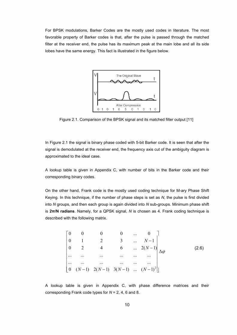
For BPSK modulations, Barker Codes are the mostly used codes in literature. The most
favorable property of Barker codes is that, after the pulse is passed through the matched
filter at the receiver end, the pulse has its maximum peak at the main lobe and all its side
lobes have the same energy. This fact is illustrated in the figure below.
Figure 2.1. Comparison of the BPSK signal and its matched filter output [11]
In Figure 2.1 the signal is binary phase coded with 5-bit Barker code. It is seen that after the
signal is demodulated at the receiver end, the frequency axis cut of the ambiguity diagram is
approximated to the ideal case.
A lookup table is given in Appendix C, with number of bits in the Barker code and their
corresponding binary codes.
On the other hand, Frank code is the mostly used coding technique for M-ary Phase Shift
Keying. In this technique, if the number of phase steps is set as N, the pulse is first divided
into N groups, and then each group is again divided into N sub-groups. Minimum phase shift
is 2π/N radians. Namely, for a QPSK signal, N is chosen as 4. Frank coding technique is
described with the following matrix.
ϕ∆
⎥⎥⎥⎥⎥
⎢⎢⎢⎢
.................................
⎥⎥⎥
⎦
⎤
⎢
⎢⎢⎢
⎣
⎡
−−−−
−−
2)1(...)1(3)1(2)1(0...
)1(2...64201...3210
0...0000
NNNN
NN
(2.6)
corresponding Frank code types for N = 2, 4, 6 and 8.
A lookup table is given in Appendix C, with phase difference matrices and their
10

There are many other coding techniques in literature such as Combined Barker (as a type of
PSK coding); Pseudorandom Codes, P1-P2-P3 and P4 codes (as types of Polyphase
mplitude, Frequency and Phase components corresponding to PMOP shapes which are
used in this thesis can be seen in Appendix A, in the PHASE MODULATION SHAPES
section
B
codes) to generate PMOP signals, but only Barker and Frank codes are considered in the
scope of this thesis.
A
11
CHAPTER 3
3. AUTOMATIC RECOGNITION OF INTRAPULSE MODULATIONS
Automatic modulation recognition algorithms mainly differ in the type of modulation they can
classify: Analog or Digital Modulation.
For analog modulation classification, readers are referred to [2]. In [2] firstly the center
frequency of the incoming signal is estimated, and then several feature extraction methods
were used for signal classification. The key features are:
• Envelope standard deviation, σa(n)
• Similarity measure of the coherent demodulation result and envelope, µ
• Difference between the standard deviation of the instantaneous frequency of
the signal and that of the squared signal, D, and
• Carrier information, C.
After extraction, these key features were given to the decision block as inputs. In the
decision block, employing suitable weighting coefficients, the Euclidean distance of these
key features with respect to all modulation types were calculated. Then the modulation type
with the smallest Euclidean distance was chosen as the correct modulation type. This
recognizer was used to discriminate between AM, FM, DSB, VSB-C, and CW modulations.
The algorithm was tested with 1500 signal segments of each 279msec time length, at SNR
levels 34.8dB, 14.8dB and 12.8dB. It is claimed that the algorithm performs over 80%
success for AM, DSB and VSB-C signals even at low SNR values. However, the algorithm
was not so powerful for AM-CW discrimination and FM-DSB discrimination at low SNRs. In
order to increase the performance of AM-CW modulation discrimination at low SNR values
an additional block was introduced to the system, which increased the success rate to 99%
at low SNR values.
Even though we gave a brief summary of recognition of analog modulations, we mainly deal
with digital modulation recognition techniques in this thesis. We also insert some additional
blocks in order to identify AM and FM analog modulations.
12
In recognition of digital modulations, there are two main approaches: “Recognition based on
the Predetection Signal itself” and “Recognition based on Features extracted from the
Predetection Signal”.
In the first approach, the aim is to group the signals of similar modulation type together from
a bunch of RF signals according to their own properties and parameters. An additional
decision block must be used after this “classification” in order to recognize the modulation
type of each class. “Maximum Likelihood Approach” [3], “Fixed-Sample-Size Classifier” [4]
and the “Fixed- Error- Rate Classifier” [4] can be listed in this type.
In the work of Boiteau and Le Martret [3], a General Maximum Likelihood Classifier (GMLC)
was introduced, based on an approximation of the likelihood function. In the classical
Maximum Likelihood (ML) approach, quasi-optimal rules were derived from the development
of the average log-likelihood function of the signal. However, that approach was only valid for
baseband pulse of duration equal to the symbol period. Boiteau and Le Martret, with the
introduction of GMLC, removed the restriction of signal duration, thus GMLC could be
applied to any baseband signal. GMLC was tested for PSK and QAM signals, and the
algorithm was also applied to M PSK / MıPSK classification. It is claimed that, test results
had shown that the GMLC approach gives equivalent result to ML tests, so GMLC provides a
general theoretical framework for the modulation recognition approach.
Lin and Kuo, worked on the sequential modulation classification of dependent samples,
using a finite state Markov Chain model [4]. They compared the Fixed-Sample-Size
Classifier and the Fixed- Error- Rate Classifier in their work. The initial one is also known as
the Likelihood Ratio Test (LRT), and uses a given fixed amount of data to decide for the
modulation type. Its performance can be measured by the average decision error probability.
The disadvantages of LRT are that the number of samples required to make decision is
related to the computational complexity and decision time delay, and that although LRT tries
to minimize the average decision error probability, it has no control on the individual error
rate.
The second one is also known as the Sequential Probability Ratio Test (SPRT), and uses a
variable amount of data just enough to achieve a certain correct ratio. This approach has
many advantages over the LRT test, such as reduced computational complexity, less
decision delay, and controllable individual classification error rate.
One of the tests was handled for classification of 8-PSK and 16-PSK, for SNR ranging from
8dB to 17dB. The claim is that, SPRT needs approximately the half of the samples to
achieve the same correct decision level with respect to LRT.
13

Another test was handled for the performance comparison of SPRT and LRT, using 8-PSK
TCM shapes. Yu-Chuan Lin and C.-C. Jay Kuo claimed that for a low SNR value of 4dB,
LRT gives 90% performance for 4-state TCM, but only 29% performance for the 2-state
TCM. Thus, although the average correct rate is at 60%, individual error rates differ in a wide
range. And the average optimum correct rate is achieved at 100 – symbol – periods. On the
other hand, SPRT gave 99% individual correct rate with the same number of symbols.
Finally, Lin and Kuo mentioned that number of symbols required for correct decision directly
affects the delay in communication links and the computational complexity. For this reason,
requiring less number of samples for correct decision, SPRT is more efficient and more
appropriate for practical use than LRT. In the second approach of digital modulation classification, the method is to extract some
features from the RF signal, and use them for recognition of the modulation type. There are
three main steps in feature based modulation recognition. In the first step preprocessing
takes place, the second is the extraction of significant features and the third is a pattern
classifier.
In the preprocessing part cyclostationarity property of signals is used. In communications
many signals have an underlying periodicity due to factors such as sampling, scanning,
modulating, multiplexing and coding. This periodicity is not always obvious. In some cases it
is hidden and then manipulation on the incoming data is necessary to bring it out.
Cyclostationarity calculations bring out this periodicity. For instance, a cyclostationary signal
of second order, is a stationary signal that exhibits second order periodicity [14].
For the feature extraction step many methods as “Constellation Shape Recognition” [5],
“Complexity Feature Extraction” [6], “Fractal Feature Extraction” [7], “Instantaneous
Frequency and Bandwidth Extraction” [8] can be listed.
Mobasseri, proposed the Constellation Shape Recognition method [5]. This method
proposes a technique that casts modulation recognition into shape recognition. In this
approach Constellation Shape is chosen as the key modulation feature. From a shape
perspective, a constellation is characterized by a particular and regular pattern of points on a
p-dimensional grid. It is the recognition and identification of this pattern that reveals the
underlying modulation. For this purpose, the proposed method firstly concentrates on
recovery of the constellation shape. The constellation of the received signal is considered as
a multidimensional random process.
14
The constellation recovery method used in the algorithm is fuzzy c-means. This is a typical
clustering algorithm, which takes the symbols taken from the signal as inputs, and in the end
outputs some key points revealing information about the modulation type of the signal, the
most important being the number and position of clusters. This knowledge is then used to
narrow down the search space of candidate modulations considerably. For each candidate
modulation, a constellation space is formed up with the samples corresponding to that
cluster. Constellation space can be thought of as a binary space; zeros everywhere except
on modulation state vectors.
For the last step in modulation classification, development of an optimal decision rule was
employed. An optimum Bayes classifier that selects the most likely modulation class based
on a single observation was selected for the classification engine. For this classification
phase, 500 instances of the reconstructed constellations for each modulation type, each
corrupted with Gaussian noise, were generated and cataloged. For the recognition step,
1000 samples of the unknown signal were processed through the constellation
reconstruction algorithm and a single constellation was recovered.
Experiments were made for various modulation standards including QPSK, 8-PSK and
16QAM. For most cases, the method has performance above 90%. This method is
consistent but is concentrated on recognition of QPSK, 8-PSK and 16QAM, which introduces
a nonflexible method.
Zhang et. al. proposed two new methods for the modulation recognition problem: Complexity
Feature Extraction Method [6] and Fractal Feature Extraction Method [7].
Complexity Feature Extraction Method [6] utilizes the Complexity Feature (CF) as the key
feature, which is composed of two other features as Lempel-Ziv complexity (LZC) and
Correlation Dimension (CD). Intra-pulse modulations of radar signals are reflected directly
on the signal waveform, as the regularity and the complexity of the waveform.
It is mentioned that the LZC can reflect the changes of phase, frequency and amplitude of a
signal, thus it is used to measure quantitatively the complexity and irregularity of radar
emitter signals. In LZC measure, only two simple operations (copy and add) are used to
describe a signal sequence and the number of required add operations is the LZC measure
value.
Fractal Theory is claimed to depict the complexity and irregularity of signals. CD is one of the
fractal dimensions, and is chosen as a classifying feature in this work for its easiness to be
obtained from signal samples directly.
15
For the simulations, ten typical modulation types as CW, BPSK, QPSK, MPSK, LFM, NLFM,
FD(Frequency Diversity), FSK, IPFE(intra-pulse frequency encoding) and CSF(Chirp
stepped-frequency) were chosen. Numerous signals were generated for different SNR
values.
Mean and variance values of LZC and CD features were calculated for each modulation
type. It is claimed that the measured values for different modulation types have obvious
separations and there is nearly no overlapping. However, variations in the features with
respect to changing SNR can not be neglected.
As mentioned above, the second method which was introduced by Zhang et. al. was the
Fractal Feature Extraction Method [7]. In this method, Box Dimension and Information
Dimension are used as classification features to recognize the types of intra-pulse
modulation of radar signals. It is claimed that Fractal dimensions can depict the complexity
and irregularity of signals quantitatively. Box dimension can reflect the geometric distribution
of a fractal set, and information dimension can reflect the distribution density of a fractal set
in space. Also it was proved that these features were insensitive to noise.
Since radar signals are time sequences, it is said that these sequences can be represented
effectively by fractal theory, and these modulation shapes can be extracted by the help of
fractal dimensions.
This method was tested with the same set of data that were used to test the Complexity
Feature Extraction Method.
Both Complexity Feature Extraction method and the Fractal Feature Extraction method are
said to recognize up to 10 different modulation types. Being insensitive to noise, the Fractal
Dimensions seem to be suitable features to use in digital modulation recognition.
Additionally, Assaleh et. al. had proposed another method in 1992 [8]. This method is the
Autoregressive Model approach, and it provides a signal representation that is convenient for
subsequent analysis. In this model the instantaneous frequency and the instantaneous
bandwidth parameters are used as the key features and these features are obtained by
using autoregressive spectrum analysis. It is said that autoregressive spectrum estimation is
an alternative to Fourier analysis for obtaining the frequency spectrum of a signal. The angle
and the magnitude terms of the poles of the autoregressive polynomial correspond to the
instantaneous frequency and instantaneous bandwidth for the signal respectively. It is
16
claimed that these features provide excellent measures for modulation type in addition to
being noise robust.
The algorithm was tested for CW, BPSK, QPSK, BFSK and QFSK signals. It is shown that
the algorithm correctly classifies modulation type at least 99% correct for an input SNR of
15dB.
In the light of knowledge above, the Fractal Feature Extraction Method [7] and the
Autoregressive Model [8] approach were chosen to form up a complete system for the
intrapulse modulation recognition problem, since both of them claim to be noise robust. The
methods and formulations are described in detail in the following chapter.
17
CHAPTER 4
4. FEATURE BASED MODULATION RECOGNITION
4.1 METHODOLOGY FOR FEATURE EXTRACTION
Mainly five parameters are selected as key features for modulation recognition in this thesis.
These features are:
• Instantaneous Frequency
• Instantaneous Bandwidth
• Box Dimension
• Information Dimension
• Percent AM Depth
The process for extracting these features is described in detail in the following sections.
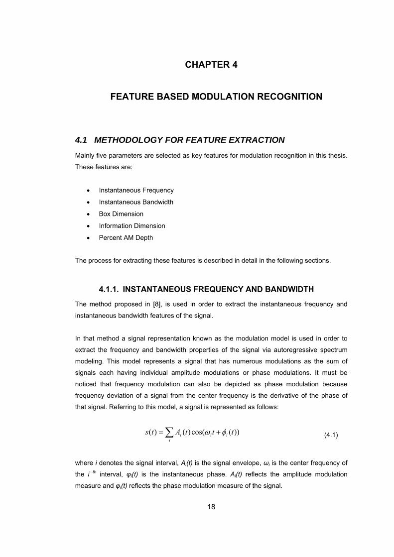
4.1.1. INSTANTANEOUS FREQUENCY AND BANDWIDTH
The method proposed in [8], is used in order to extract the instantaneous frequency and
instantaneous bandwidth features of the signal.
In that method a signal representation known as the modulation model is used in order to
extract the frequency and bandwidth properties of the signal via autoregressive spectrum
modeling. This model represents a signal that has numerous modulations as the sum of
signals each having individual amplitude modulations or phase modulations. It must be
noticed that frequency modulation can also be depicted as phase modulation because
frequency deviation of a signal from the center frequency is the derivative of the phase of
that signal. Referring to this model, a signal is represented as follows:
∑ +=i
iii tttAts ))(cos()()( φω (4.1)
where i denotes the signal interval, Ai(t) is the signal envelope, ωi is the center frequency of
the i th interval, φi(t) is the instantaneous phase. Ai(t) reflects the amplitude modulation
measure and φi(t) reflects the phase modulation measure of the signal.
18
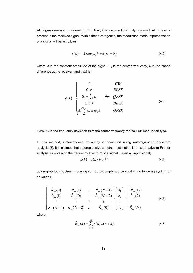
AM signals are not considered in [8]. Also, it is assumed that only one modulation type is
present in the received signal. Within these categories, the modulation model representation
of a signal will be as follows:
))(cos()( θφω ++= kkAks c (4.2)
where A is the constant amplitude of the signal, ωc is the center frequency, θ is the phase
difference at the receiver, and Ф(k) is:
⎪⎪⎪
⎩
⎪⎪⎪
⎨
⎧
±±
±
±=
QFSKkk
BFSKk
QPSKfor
BPSKCW
k
dd
d
ωω
ω
πππ
φ
,2
,2
,0
,00
)(
(4.3)
Here, ωd is the frequency deviation from the center frequency for the FSK modulation type.
In this method, instantaneous frequency is computed using autoregressive spectrum
analysis [8]. It is claimed that autoregressive spectrum estimation is an alternative to Fourier
analysis for obtaining the frequency spectrum of a signal. Given an input signal;
)()()( knkskx += (4.4)
autoregressive spectrum modeling can be accomplished by solving the following system of
equations;
⎥⎥⎥⎥⎥
⎦
⎤
⎢⎢⎢⎢⎢
⎣
⎡
=
⎥⎥⎥⎥
⎦
⎤
⎢⎢⎢⎢
⎣
⎡
⋅
⎥⎥⎥⎥⎥
⎦
⎤
⎢⎢⎢⎢⎢
⎣
⎡
−−
−−
)(ˆ
)2(ˆ)1(ˆ
)0(ˆ)2(ˆ)1(ˆ
)2(ˆ)0(ˆ)1(ˆ)1(ˆ)1(ˆ)0(ˆ
2
1
NR
RR
a
aa
RNRNR
NRRRNRRR
xx
xx
xx
Nxxxxxx
xxxxxx
xxxxxx
MM
K
MOMM
K
K
(4.5)
where,
∑ +=M
=xx knxnxkR )().()(ˆ (4.6)
n 0
19
Here M is the number of samples existing in the analysis frame, and a is a vector that
represents the coefficients for the polynomial that best fits the frequency spectrum. Phase of
a pole of this polynomial corresponds to the frequency of that signal, and the magnitude of a
ole corresponds to the bandwidth of that signal. These relations are given with the following
formula;
p
⎥⎦
⎤⎢⎣
⎡== −
)Re()Im(
tan22
1
i
isi
si Z
ZFFF
πθ
π (4.7)
nd a
⎥⎦
⎤⎢⎣
⎡+
−= 2210 )Re()Im(1log10
ii
si ZZ
FBW
π (4.8)
where F is the instantaneoui s frequency and BWi is the instantaneous bandwidth of the
sponding samples in the analysis frame, is the sampling rate, θ is the phase angle
of these segments is called an “instant” of the signal.
Fi and BWi values are calculated for all these signal segments. The concatenation of
these in bandwidth
4.1.2. BOX DIMENSION AND INFORMATION DIMENSION
ox dimension
c shape that can be subdivided in parts,
- are most
or irregularity
over multiple scales. (Modulation creates irregularities on the signal waveform.)
corre Fs i
between the real and imaginary components of Zi, and Zi is the i th complex pole of the
autoregressive polynomial.
In the beginning of these calculations, the whole signal is partitioned into overlapping
analysis frames of a fixed length. Each
Then,
stantaneous frequency and bandwidth values reflects the frequency and
properties of the corresponding pulse.
The metho
and information dimension features of the signal.
d proposed in [7], employs Fractal Theory in order to extract the b
First of all, a brief information about Fractal Theory should be given [9]:
Fractals are of rough or fragmented geometri-
each of which is (at least approximately) a reduced copy of the whole.
They are crinkly objects that defy conventional measures, such as length and
often characterized by their fractal dimension.
- Fractal Dimension measures the degree of fractal boundary fragmentation
- Fractal Dimensions are relatively insensible to image scaling.
- Very often, fractal dimension is a quite unique classifier for similar shapes.
20
Thus, if we consider a signal, as a composition of infinitely small fractals, we can represent
the “length” of this signal and the irregularities in the signal in terms of its fractal dimensions.
he last two bullets confirm that fractal dimensions correctly fit the aim of modulation
tion shapes.
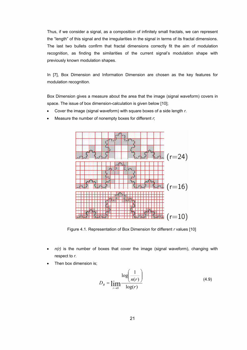
age (signal waveform) covers in
pace. The issue of box dimension-calculation is given below [10];
• Cover the image (signal waveform) with square boxes of a side length r.
• Measure the number of nonempty boxes for different r;
T
recognition, as finding the similarities of the current signal’s modulation shape with
previously known modula
In [7], Box Dimension and Information Dimension are chosen as the key features for
modulation recognition.
Box Dimension gives a measure about the area that the im
s
Figure 4.1. Representation of Box Dimension for different r values [10]
• n(r) is the number of boxes that cover the image (signal waveform), chang th
respect to r.
ing wi
• Then box dimension is;
)log()(
log
lim0 r
rnD
rB
⎟⎟⎠
⎜⎜⎝=
→
(4.9)
1 ⎞⎛
21
The
the oposed;
ete time
sequence. By Fourier transform the signal is transformed to a discrete signal in
frequency domain. Then the energy of the signal is normalized so that the effect of the
distance of radar emitter and the signal is eliminated.
- After the signal preprocessing, the sequence g(i) is obtained. Then, for a certain box
}
description above is given for images, and this calculation method must be adapted to
signal waveform case. In [7], the following method is pr
- First of all the signal is passed through a preprocess. In this phase the signal is
transformed to a sequence in frequency domain. The received signal is a discr
size, the number of boxes that cover the signal waveform N(q) is calculated as;
{ } {2
1
1 1)(q
NqN i i ⎦⎣+= = =
where N is the length of the sequence, and q is the size of the boxes chosen to cover the
signal.
Investigating the formula, we see that if the signal had constant value through all
samples, only N boxes would be sufficient to cover the s
1
)1(),(min)1(),(max qigigqigigN N
⎥⎤
⎢⎡
+−+∑ ∑− −
(4.10)
ignal in space. Then,
onsidering the discontinuities found in the signal shape, the second part of the addition
rm is obtained.
Fs is the sampling rate.
This is because the signal is composed of samples each 1/Fs seconds apart. A larger
box size selection would result in data loss and a smaller box size selection would
require interpolation between two real samples.
c
is generated. This part calculates the absolute difference between two consecutive
samples of the signal and calculates the number of boxes of size q that will cover this
difference. Making this calculation for all consecutive samples of the signal, the total
number of boxes that will cover the signal wavefo
After certain trials the ideal box size is found as q = 1/Fs, where
- After the calculation of N(q), the box dimension is calculated as;
qb ln
qN )( (4.11)
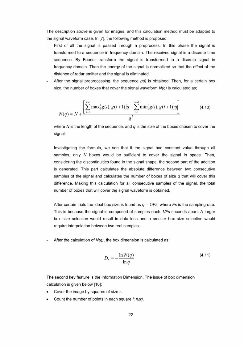
The second key feature is the Information Dimension. The issue of box dimension
calculation is given below [10];
• Cover the image by squares of size r.
• Count the number of points in each square i; ni(r).
D ln−=
22
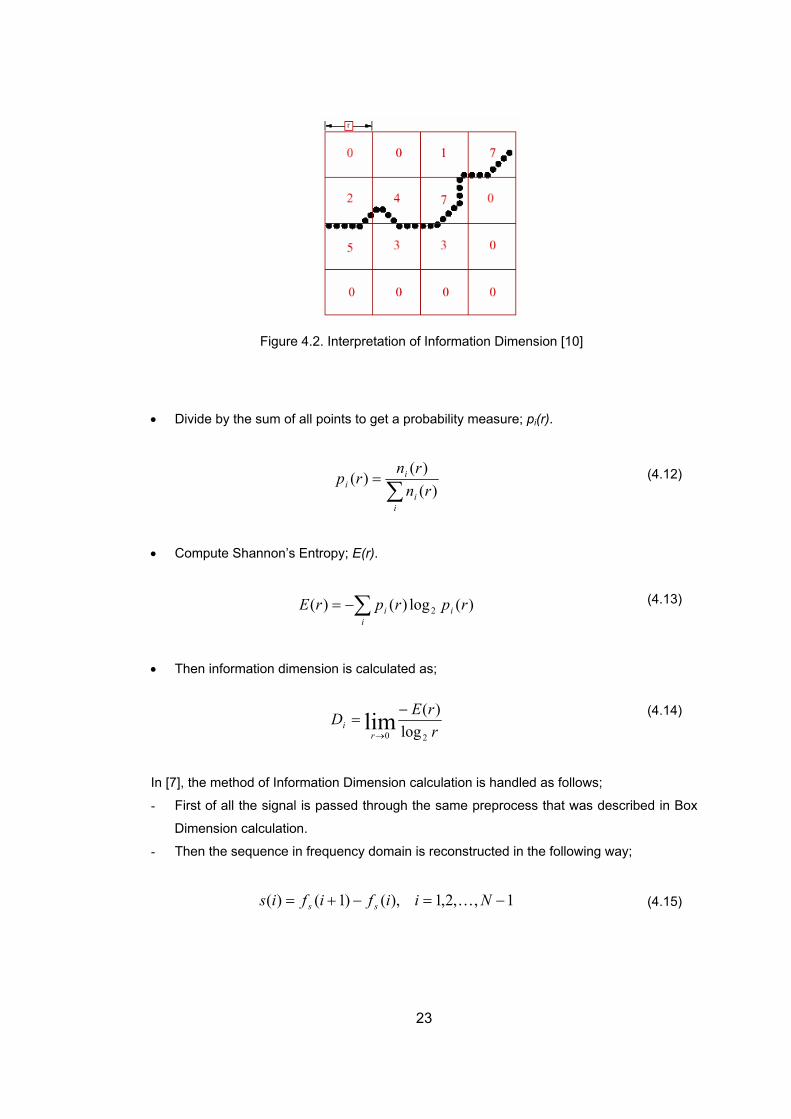
Figure 4.2. Interpretation of Information Dimension [10]
Divide by the sum of all points to get a probability measure; pi(r).
•
∑=
ii
ii rn
rnrp
)()(
)( (4.12)
• Compute Shannon’s Entropy; E(r).
i
)(log)()( 2 rprprE ii∑−= (4.13)
• Then information dimension is calcul ed as;
at
rri
20 logrED )(lim −
= (4.14)
In [7 tion Dimension calculation is handled as follows;
ed in Box
Dimension calculation.
- Then the sequence in frequency domain is reconstructed in the following way;
→
], the method of Informa
- First of all the signal is passed through the same preprocess that was describ
1,,2,1),()1()( −=−+= Niififis ss K (4.15)
23
Authors claim that this reconstruction method can eliminate a part of noise. Since the
noise in our system is AWGN, it is spread overall the frequency spectrum, thus by
differentiating the signal we can reduce the effect of this noise by a certain amount.
- Finally, Information dimension is calculated by using the following formula e
y domain signal.
(4.16)
where,
s in th
frequenc
∑−
=
=1
1)/1log(.
N
iiii PPD
∑−
=
=1
1
N
iisL (4.17)
Ls
P ii = (4.18)
ere si is the reconstructed signal, N is the length of the signal, and Pi is the probability
ox
Dimension calculations. This choice eliminates the usage of the limit function present in
ult it is seen that Box Dimension of a fractal set can reflect the geometric distribution,
nd Information Dimension can reflect the distribution density of the fractal set in space.
nd are not easily affected by
noise.
In the figure below, we can see the distribution of fractal dimensions among various
modulation types. It is seen that Box Dimension and Information dimension give a useful
measure for distinguishing between different modulation types.
H
that all the irregularities present in the signal can be represented by the corresponding
individual irregularity, si. Here, the box size is chosen as q=1/Fs, same as the B
the definition of Information Dimension.
As a res
a
It is claimed by the authors that these features, reflecting the complexity and irregularity of
the radar signal, depict the modulation property of that signal a
24
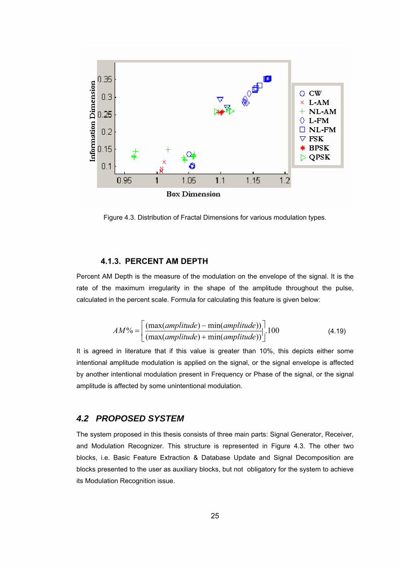
Figure 4.3. Distribution of Fractal Dimensions for various modulation types.
4.1.3. PERCENT AM DEPTH
Percent AM Depth is the measure of the modulation on the envelope of the signal. It is the
rate of the maximum irregularity in the shape of the amplitude throughout the pulse,
calculated in the percent scale. Formula for calculating this feature is given below:
100.))min()(max(
% ⎥⎦
⎢⎣ +
=amplitudeamplitude
AM (4.19)
It is agreed in literature that if this value is greater than 10%, this depicts either some
intentional amplitude modulation is applied on the signal, or the signal envelope is affected
by another intentional modulation present in Frequency o
))min((max( ⎤⎡ − amplitudeamplitude
r Phase of the signal, or the signal
mplitude is affected by some unintentional modulation.
xiliary blocks, but not obligatory for the system to achieve
s Modulation Recognition issue.
)
a
4.2 PROPOSED SYSTEM
The system proposed in this thesis consists of three main parts: Signal Generator, Receiver,
and Modulation Recognizer. This structure is represented in Figure 4.3. The other two
blocks, i.e. Basic Feature Extraction & Database Update and Signal Decomposition are
blocks presented to the user as au
it
25
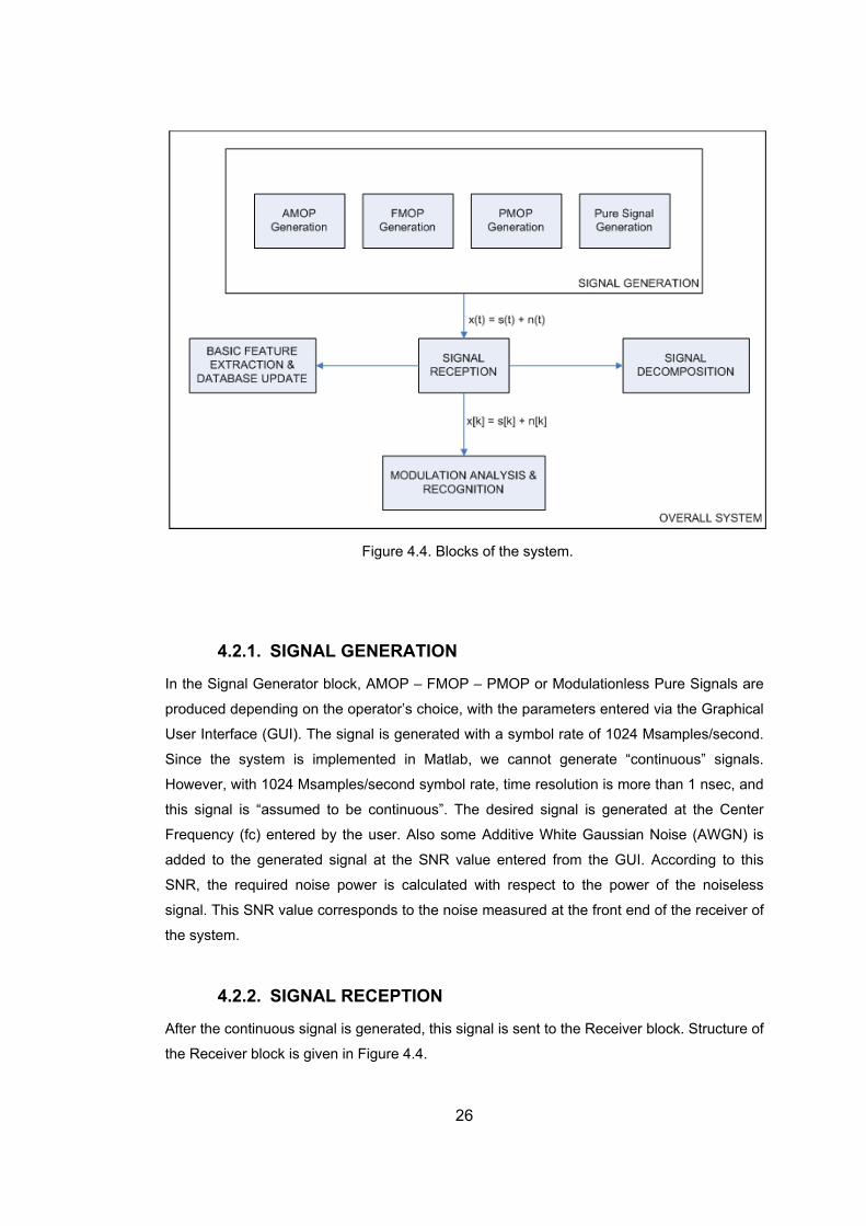
Figure 4.4. Blocks of the system.
NR value corresponds to the noise measured at the front end of the receiver of
e system.
is signal is sent to the Receiver block. Structure of
e Receiver block is given in Figure 4.4.
4.2.1. SIGNAL GENERATION
In the Signal Generator block, AMOP – FMOP – PMOP or Modulationless Pure Signals are
produced depending on the operator’s choice, with the parameters entered via the Graphical
User Interface (GUI). The signal is generated with a symbol rate of 1024 Msamples/second.
Since the system is implemented in Matlab, we cannot generate “continuous” signals.
However, with 1024 Msamples/second symbol rate, time resolution is more than 1 nsec, and
this signal is “assumed to be continuous”. The desired signal is generated at the Center
Frequency (fc) entered by the user. Also some Additive White Gaussian Noise (AWGN) is
added to the generated signal at the SNR value entered from the GUI. According to this
SNR, the required noise power is calculated with respect to the power of the noiseless
signal. This S
th
4.2.2. SIGNAL RECEPTION
After the continuous signal is generated, th
th
26
Figure 4.5. Receiver block of the system
In the Receiver block, continuous signal is first carried to the Intermediate Frequency (IF). IF
of the system is 160 MHz. In this process, we assume that the center frequency of the
incoming signal is known. In real systems, the center frequency of the signal can be
extracted with a precision rate of a few kHz, thus our assumption does not diverge from the
27
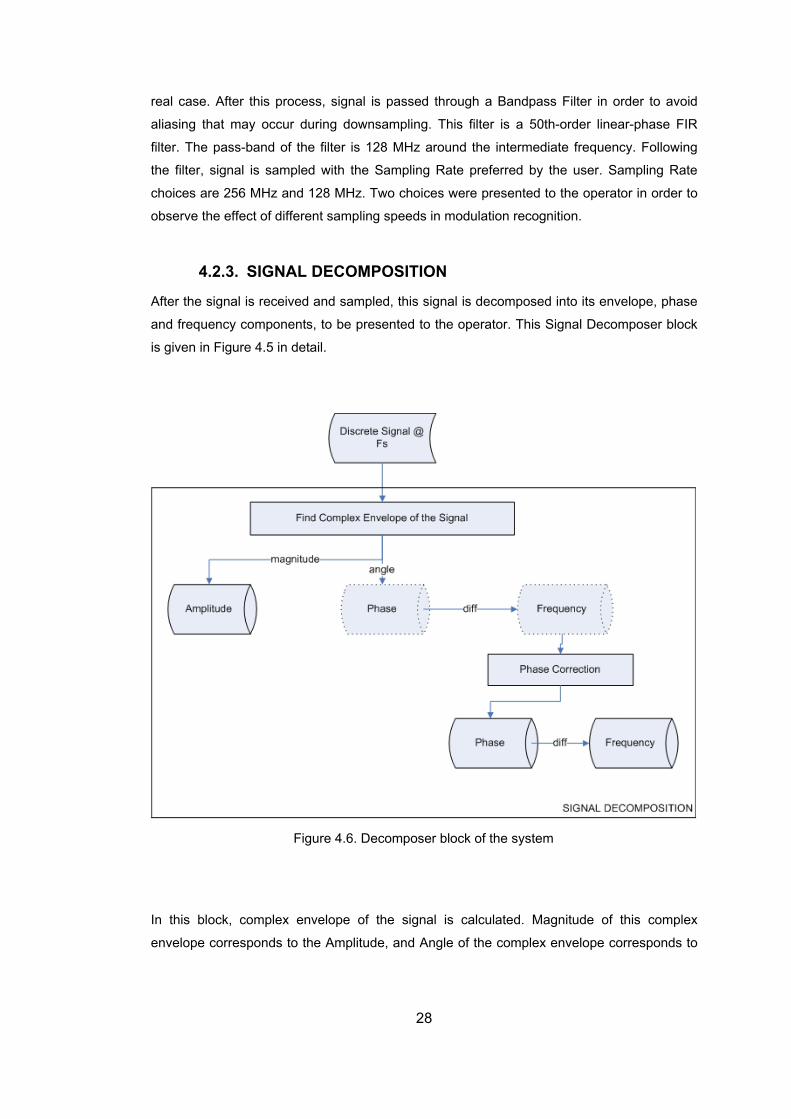
real case. After this process, signal is passed through a Bandpass Filter in order to avoid
aliasing that may occur during downsampling. This filter is a 50th-order linear-phase FIR
filter. The pass-band of the filter is 128 MHz around the intermediate frequency. Following
the filter, signal is sampled with the Sampling Rate preferred by the user. Sampling Rate
choices are 256 MHz and 128 MHz. Two choices were presented to the operator in order to
observe the effect of different sampling speeds in modulation recognition.
4.2.3. SIGNAL DECOMPOSITION
After the signal is received and sampled, this signal is decomposed into its envelope, phase
and frequency components, to be presented to the operator. This Signal Decomposer block
is given in Figure 4.5 in detail.
Figure 4.6. Decomposer block of the system
In this block, complex envelope of the signal is calculated. Magnitude of this complex
envelope corresponds to the Amplitude, and Angle of the complex envelope corresponds to
28

the Phase of the signal. Frequency of the signal is found by differentiating the Phase of the
signal.
Throughout the algorithms, it is assumed that we know the center frequency of the original
signal. However, if there were some discrepancy between the original center frequency
value and the extrac er frequency value, this effect would be seen in the output of the
Decomposer block as a deviation in the Pulse Frequency from the IF. Taking this probability
into account, Phase the pulse is corrected according to the deviation of mean of the
xtracted Pulse Frequency from IF. For this purpose the following method is used;
ted cent
of
e
)0( >FIf
( )( ) 0
01 sintan_ ωω
ωωωω
+=⎟⎟⎞
⎜⎜⎝
⎛++
= −c
cPhaseCorrected
0cos ⎠c
( )( ) 0
01
costan_ ωω
ωω−=⎟⎟
⎠⎜⎜⎝ −
= −c
cPhaseCorrected0
sin
c
)0(
ωω ⎞⎛ −
<FIf
where,
( )
( )
[ ]NF
FRateSamplingF
PulsetheinsamplesofNumberPulselengthNValuesPhasePulse
IFfromDeviationIFFreqPulsemeanF
s
s
c
L212
_
0 ⋅=
=⇒=
=⇒−=
πω
ω
Phase of the Pulse is corrected with the method described above, and the Frequency of the
pulse is calculated again due to this corrected phase.
At this point, there are two preferences for the user: “Basic Feature Extraction & Database
Update” or “Modulation Analysis & Recognition”.
4.2.4. BASIC FEATURE EXTRACTION AND DATABASE UPDATE
User may choose to analyze the signal step by step and save the analysis results in the
IMOP database.
29
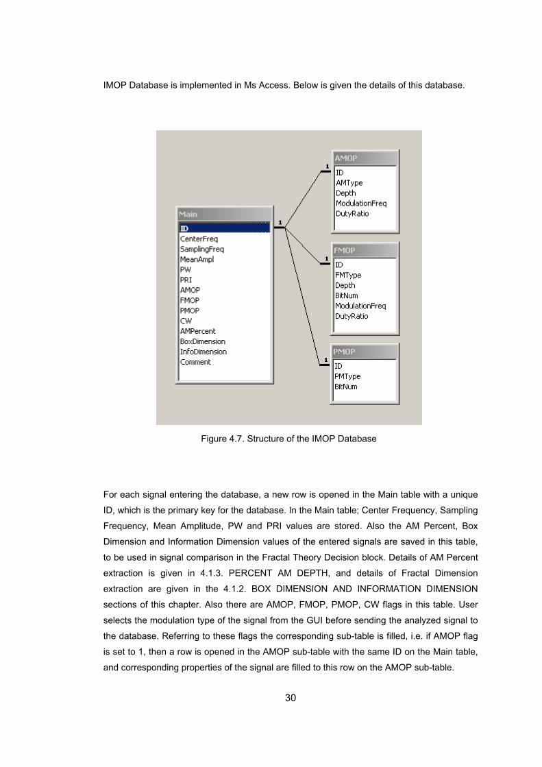
IMOP Database is implemented in Ms Access. Below is given the details of this database.
Figure 4.7. Structure of the IMOP Database
For each signal entering the database, a new row is opened in the Main table with a unique
ID, which is the primary key for the database. In the Main table; Center Frequency, Sampling
Frequency, Mean Amplitude, PW and PRI values are stored. Also the AM Percent, Box
Dimension and Information Dimension values of the entered signals are saved in this table,
to be used in signal comparison in the Fractal Theory Decision block. Details of AM Percent
extraction is given in 4.1.3. PERCENT AM DEPTH, and details of Fractal Dimension
extraction are given in the 4.1.2. BOX DIMENSION AND INFORMATION DIMENSION
sections of this chapter. Also there are AMOP, FMOP, PMOP, CW flags in this table. User
elects the modulation type of the signal from the GUI before sending the analyzed signal to
b-table.
s
the database. Referring to these flags the corresponding sub-table is filled, i.e. if AMOP flag
is set to 1, then a row is opened in the AMOP sub-table with the same ID on the Main table,
and corresponding properties of the signal are filled to this row on the AMOP su
30

As mentioned in the preceding paragraph, there are sub-tables related to the Main table with
the ID parameter. This relationship is 1-1, thus an element in the AMOP table can be related
to only one element that has the same ID in the Main table.
AM Type, AM Depth, Modulation Frequency and Duty Ratio fields exist in the AMOP sub-
table. AM Type can be “Linear-Increasing”, “Linear-Decreasing”, “Positive Parabolic”,
egative Parabolic”, ”Sinusoidal”, ”Triangular”, “Ramp” or ”Square”. AM Depth value is valid
rabolic”, “Negative Parabolic”, ”Sinusoidal”, ”Triangular”, “Ramp”,
quare” or “BFSK”. FM Depth value is valid for all these types, however “Modulation
modulation is ”Square”, and “BitNum” field is filled if
e modulation is BFSK.
code) fields exist in the PMOP sub-
ble. PM Type can be BPSK or MPSK.
gh to totally describe the CW signal.
On the oth ncoming signal
without Analyzer and
4.2.5. MODULATION ANALYSIS AND RECOGNITION
Details of the Mod
“N
for all these types, however “Modulation Frequency” field is filled if the modulation is Periodic
(”Sinusoidal”, ”Triangular”, “Ramp” or ”Square”), and “Duty Ratio” field is filled if the
modulation is ”Square”.
FM Type, FM Depth, BitNum (Number of Bits in the modulating code), Frequency and Duty
Ratio fields exist in the FMOP sub-table. FM Type can be “Linear-Increasing”, “Linear-
Decreasing”, “Positive Pa
”S
Frequency” field is filled if the modulation is Periodic (”Sinusoidal”, ”Triangular”, “Ramp” or
”Square”), “Duty Ratio” field is filled if the
th
PM Type and BitNum (Number of Bits in the modulating
ta
There is no sub-table for the “No Modulation” or “CW” case, because the parameters in the
Main table are enou
er hand, if the user chooses to find the modulation type of the i
making manual analysis, the signal is sent to the Modulation
Recognizer block.
ulation Recognition block is given in Figure 4.7.
31
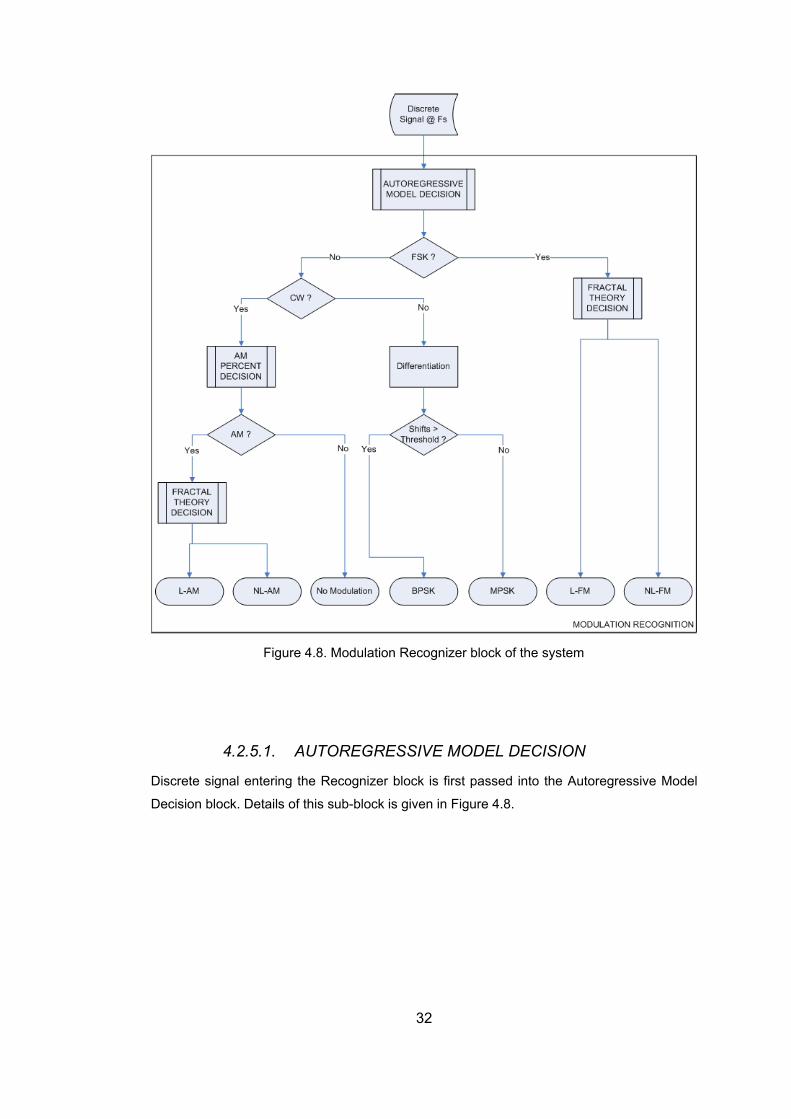
Figure 4.8. Modulation Recognizer block of the system
4.2.5.1. AUTOREGRESSIVE MODEL DECISION
Discrete signal entering the Recognizer block is first passed into the Autoregressive Model
Decision block. Details of this sub-block is given in Figure 4.8.
32
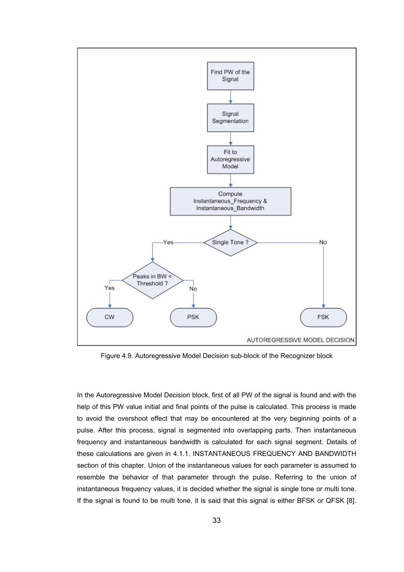
Figure 4.9. Autoregressive Model Decision sub-block of the Recognizer block
ered at the very beginning points of a
ulse. After this process, signal is segmented into overlapping parts. Then instantaneous
n of this chapter. Union of the instantaneous values for each parameter is assumed to
semble the behavior of that parameter through the pulse. Referring to the union of
instantaneous frequency values, it is decided whether the signal is single tone or multi tone.
If the signal is found to be multi tone, it is said that this signal is either BFSK or QFSK [8].
In the Autoregressive Model Decision block, first of all PW of the signal is found and with the
help of this PW value initial and final points of the pulse is calculated. This process is made
to avoid the overshoot effect that may be encount
p
frequency and instantaneous bandwidth is calculated for each signal segment. Details of
these calculations are given in 4.1.1. INSTANTANEOUS FREQUENCY AND BANDWIDTH
sectio
re
33
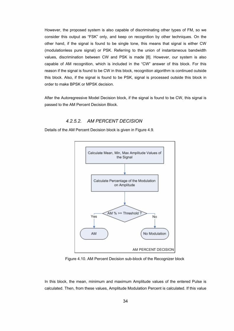
However, th g other types of FM, so we
ther techniques. On the
ther hand, if the signal is found to be single tone, this means that signal is either CW
algorithm is continued outside
this block. Als i found to be PSK, signal is processed outside this block in
order to make BPSK or MPSK dec
oreg ck, if the signal is found to be CW, this signal is
e proposed system is also capable of discriminatin
consider this output as “FSK” only, and keep on recognition by o
o
(modulationless pure signal) or PSK. Referring to the union of instantaneous bandwidth
values, discrimination between CW and PSK is made [8]. However, our system is also
capable of AM recognition, which is included in the “CW” answer of this block. For this
reason if the signal is found to be CW in this block, recognition
o, f the signal is
ision.
After the Aut ressive Model Decision blo
passed to the AM Percent Decision Block.
4.2.5.2. AM PERCENT DECISION
Details of the AM Percent Decision block is given in Figure 4.9.
Figure 4.10. AM Per Recognizer block
this block, the mean, minimum and maximum Amplitude values of the entered Pulse is
calculated. Then, from these values, Amplitude Modulation Percent is calculated. If this value
cent Decision sub-block of the
In
34
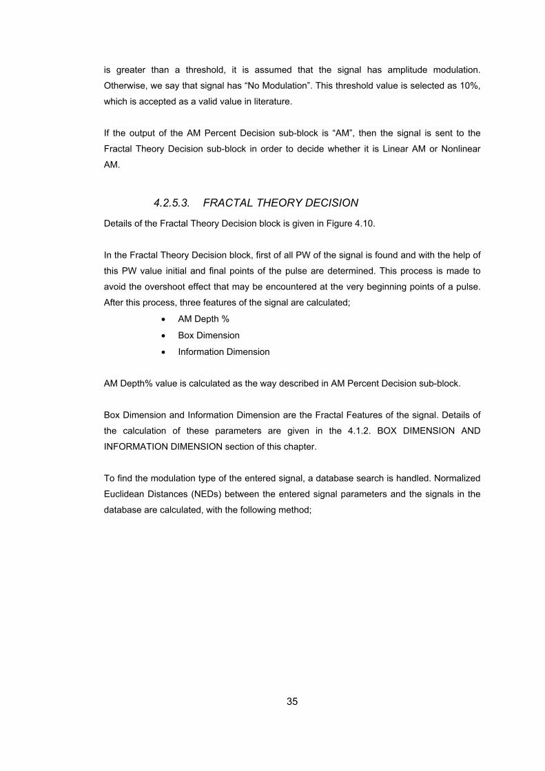
is greater than a threshold, it is assumed that the signal has amplitude modulation.
Otherwise, we say that signal has “No Modulation”. This threshold value is selected as 10%,
which is accepted as a valid value in literature.
Decision block is given in Figure 4.10.
itial and final points of the pulse are determined. This process is made to
void the overshoot effect that may be encountered at the very beginning points of a pulse.
After this process, three features of the signal are calculated;
• Information Dimension
M Depth% value is calculated as the way described in AM Percent Decision sub-block.
e calculation of these parameters are given in the 4.1.2. BOX DIMENSION AND
malized
uclidean Distances (NEDs) between the entered signal parameters and the signals in the
If the output of the AM Percent Decision sub-block is “AM”, then the signal is sent to the
Fractal Theory Decision sub-block in order to decide whether it is Linear AM or Nonlinear
AM.
4.2.5.3. FRACTAL THEORY DECISION
Details of the Fractal Theory
In the Fractal Theory Decision block, first of all PW of the signal is found and with the help of
this PW value in
a
• AM Depth %
• Box Dimension
A
Box Dimension and Information Dimension are the Fractal Features of the signal. Details of
th
INFORMATION DIMENSION section of this chapter.
To find the modulation type of the entered signal, a database search is handled. Nor
E
database are calculated, with the following method;
35
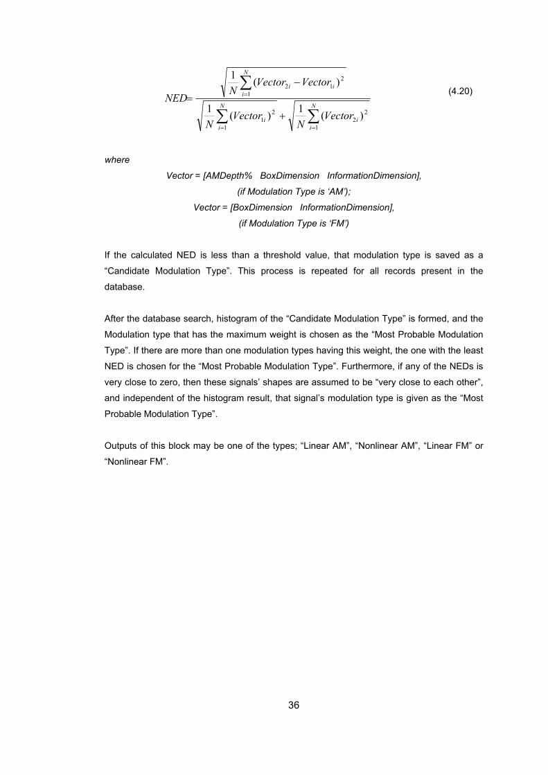
2
11 == ii 2
21
2
1
)()(1
)(1
∑∑
∑=
+
=N
i
N
i
N
i
VectorVectorN
NNED
(4.20)
here
e is ‘AM’);
Vector = [BoxDimension InformationDimension],
(if Modulation Type is ‘FM’)
If the calculated NED is less than a threshold value, that modulation type is saved as a
type is given as the “Most
robable Modulation Type”.
12 − ii VectorVector
1N
w
Vector = [AMDepth% BoxDimension InformationDimension],
(if Modulation Typ
“Candidate Modulation Type”. This process is repeated for all records present in the
database.
After the database search, histogram of the “Candidate Modulation Type” is formed, and the
Modulation type that has the maximum weight is chosen as the “Most Probable Modulation
Type”. If there are more than one modulation types having this weight, the one with the least
NED is chosen for the “Most Probable Modulation Type”. Furthermore, if any of the NEDs is
very close to zero, then these signals’ shapes are assumed to be “very close to each other”,
and independent of the histogram result, that signal’s modulation
P
Outputs of this block may be one of the types; “Linear AM”, “Nonlinear AM”, “Linear FM” or
“Nonlinear FM”.
36
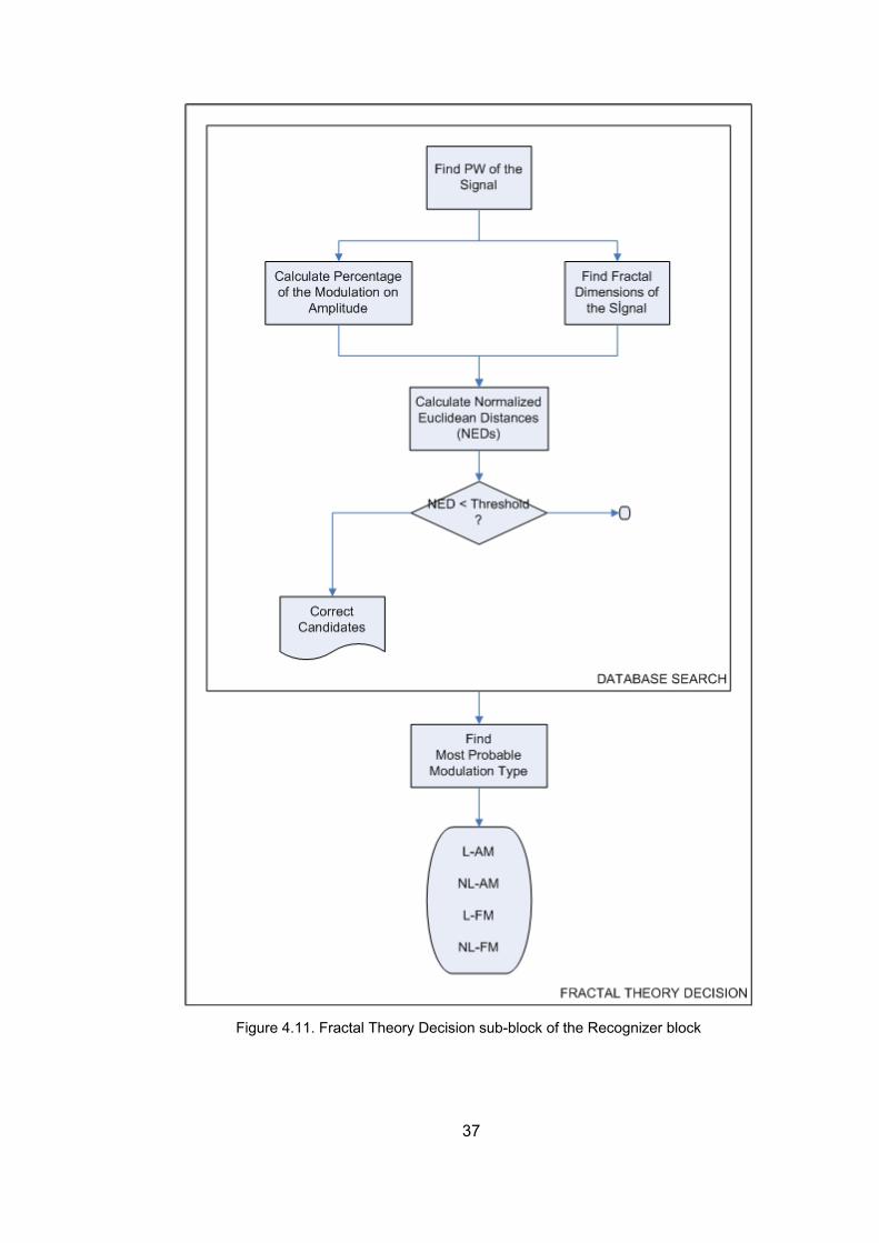
Figure 4.11. Fractal Theory Decision sub-block of the Recognizer block
37
If the output of the AM Percent Decision sub-block is “No Modulation”, then no further
processing is required; signal is said to have no modulation, i.e. the signal is a pure sinusoid.
If the ou sub-block is “PSK”, then the Phase of the
pulse is differentiated. If any of ss than π radians, the signal is said to
By the help of this block, the signal is decided
hether it is Linear FM or Nonlinear FM.
resented to the user. Details about this interface is given in Appendix B.
tput of the Autoregressive Model Decision
the differences is le
have MPSK modulation. Otherwise the signal is decided to have BPSK modulation.
After the Autoregressive Model Decision block, if the signal is found to be FSK, this signal is
passed to the Fractal Theory Decision Block.
w
In order to make the simulations of the proposed system easier, a graphical user interface is
also designed and p
38
CHAPTER 5
5. PERFORMANCE TESTS In order to test the performance of the system, computer simulations were carried out using
the Graphical User Interface created in MATLAB.
5.1. SIGNAL TYPES USED IN SIMULATIONS
Proposed algorithm was tested for AMOP, FMOP, PMOP modulation types and for signals
without modulation. All signals were constructed using MATLAB programming language.
ignals were constructed at the given center frequency with a symbol rate of 1024MHz at
rst, so that they could be assumed to be continuous signals coming to the receiver of the
entered from the User Interface. This SNR value corresponds to the
oise measured at the front end of the receiver of the system.
In the re was
recovered
the as cho 60MHz. e that the cente ncy
of the incoming signal is known. In uency of the signal can be
xtrac h a precisi kHz, thu doe t dive
mpling in order to avoid aliasing. This filter was
esigned with the “fir1” command of Matlab. Filtered signal was then sampled at one of the
esponding variable parameters used in the performance tests
re given in Table 5.1.
S
fi
system from the surrounding, with approximately 1nsec time resolution. In order to model the
noise effects, Additive White Gaussian Noise was generated and added to the incoming
signal, at the SNR value
n
ceiver part of the system, it is assumed that center frequency of the signal
correctly and the signal was moved to the intermediate frequency (IF). IF value for
system w sen to be 1 In this process, we assum r freque
real systems, the center freq
s our assumption e ted wit on rate of a few s no rge from the
real case.
The signal at IF which was assumed to resemble the continuous signal model, was filtered
with a 50th order Bandpass filter, before sa
d
two different Sampling Frequency (Fs) choices, depending on the user selection. Fs values
offered to the user were 256MHz and 128MHz respectively.
Modulation Types and the corr
a
39
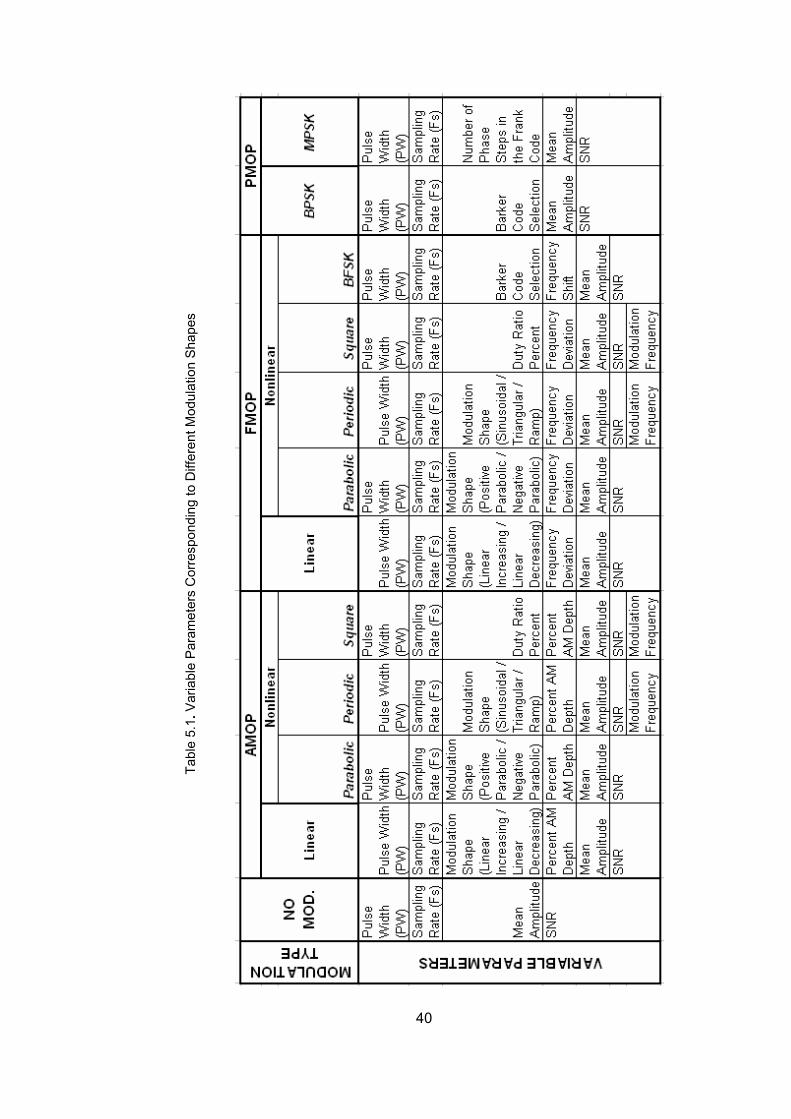
Tabl
e 5.
1. V
ara
met
ers
Cor
resp
ondi
ng to
Diff
eren
t Mod
ulat
s io
n S
hape
riabl
e P
a
40
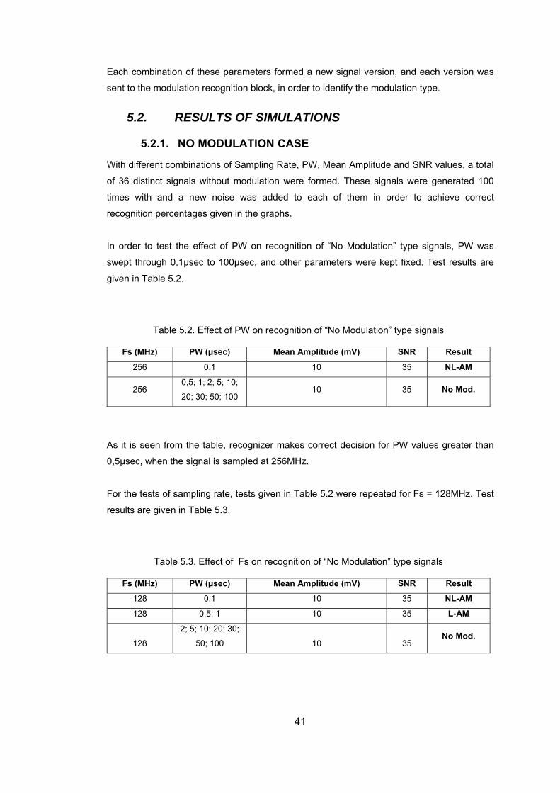
Each combination of these parameters formed a new signal version, and each version was
sent to the modulation recognition block, in order to identify the modulation type.
ith different combinations of Sampling Rate, PW, Mean Amplitude and SNR values, a total
of 36 distinct signals without modulation were formed. These signals were generated 100
times with and a ne chieve correct
recognition percentages given in the graphs.
In order to tes t of PW on rec f “N lation” gnal s
swept through 0,1µsec to 100µsec, and other parameters were kept fixed. Test results are
given in Table 5.2.
Table 5.2. Effect of PW on recog of “No M ulation” type signals
Fs (MHz) PW (µsec) Mean Amplitude (mV) SNR Result
5.2. RESULTS OF SIMULATIONS
5.2.1. NO MODULATION CASE
W
w noise was added to each of them in order to a
t the effec ognition o o Modu type si s, PW wa
nition od
256 0,1 10 35 NL-AM
256 0,5; 1; 2; 5; 10;
20; 30; 50; 100 10 35 No Mod.
As it is seen from the table, recognizer makes correct decision for PW values greater than
0,5µsec, when the signal is sampled at 256MHz.
For the tests of s = 128MHz. Test
results are given in Table 5.3.
Table 5.3. Effect of Fs on recognition o odulation” type sig
Hz) Mean Ampl mV) SNR Re
ampling rate, tests given in Table 5.2 were repeated for Fs
f “No M nals
Fs (M PW (µsec) itude ( sult
128 0,1 10 35 NL-AM
128 ,5; 1 10 35 L-0 AM
128 50; 100 10 35 No Mod.
2; 5; 10; 20; 30;
41
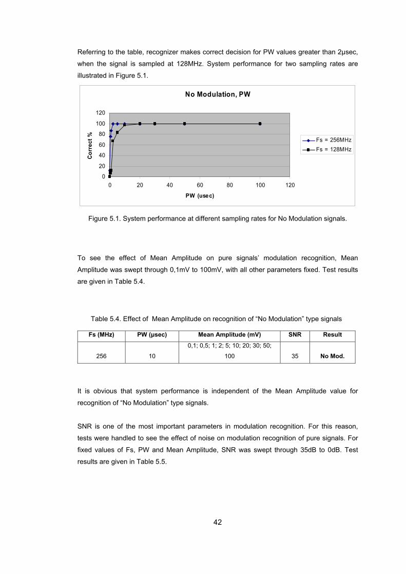
Referring to the table, recognizer makes correc cision for PW values greater than 2µsec,
when the signal is sampled at 128MHz. System performance for two sampling rates are
illustrated in Figure 5.1.
t de
No Modulation, PW
0
20
40
60
80
100
120
0 20 40 60 80 100 120
PW (usec)
Corr
ect % Fs = 256MHz
Fs = 128MHz
o see the effect of Mean Amplitude on pure signals’ modulation recognition, Mean
mplitude was swept through 0,1mV to 100mV, with all other parameters fixed. Test results
are give
le 5.4. t of Mean Amplitude on reco of “No dulatio pe si
Hz) PW (µsec) Mean Am (mV) SN
Figure 5.1. System performance at different sampling rates for No Modulation signals.
T
A
n in Table 5.4.
Tab Effec gnition Mo n” ty gnals
Fs (M plitude R Result
256 10
0; 30; 5
100 35 N0,1; 0,5; 1; 2; 5; 10; 2 0;
o Mod.
is vious th ystem perfor ce is indep ude value for
n of “No Modulation” type signals.
SNR is one of the most important parameters in modulation recognition. For this reason,
tests were handled to see the effect of noise on modulation recognition of pure signals. For
fixed values of Fs, PW and Mean Amplitude, SNR was swept through 35dB to 0dB. Test
results are given in Table 5.5.
It ob at s man endent of the Mean Amplit
recognitio
42
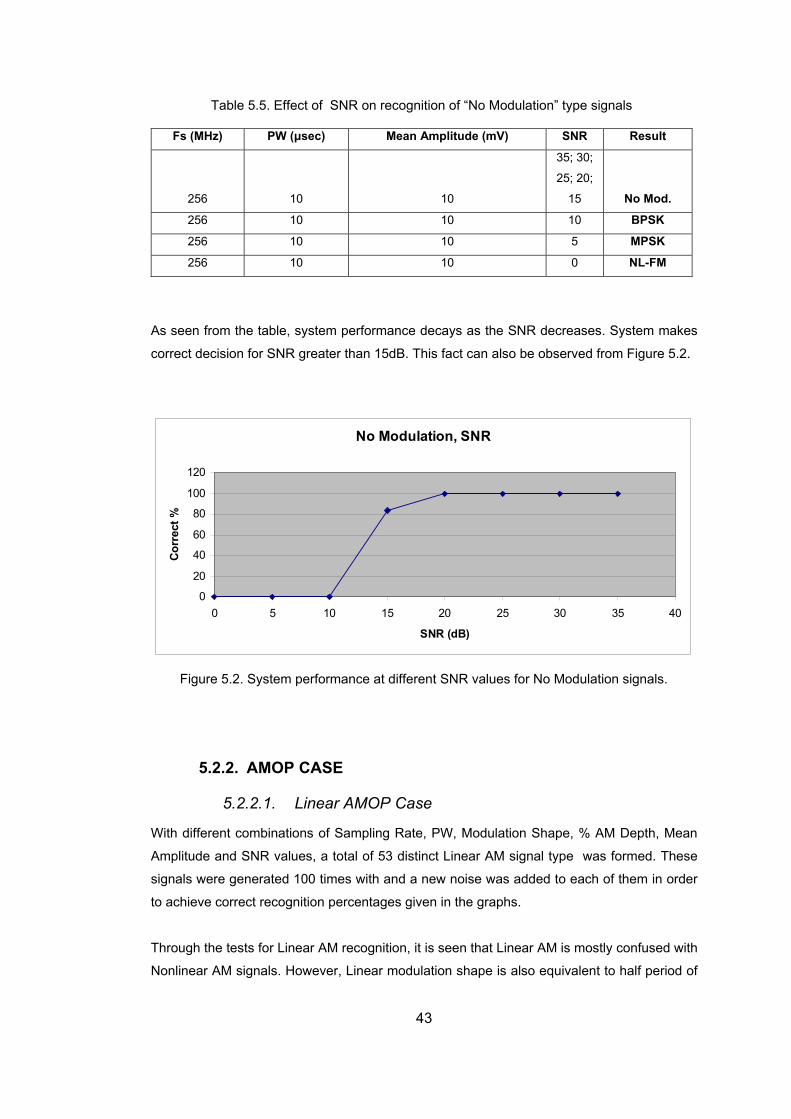
Table 5.5. Effect of SNR on recognition of “No Modulation” type signals
Fs (MHz) PW (µsec) Mean Amplitude (mV) SNR Result
256 10 10
35; 30;
25; 20;
15 No Mod.
256 10 10 10 BPSK
256 10 10 5 MPSK
256 10 10 0 NL-FM
As seen from the table, system performance decays as the SNR decreases. System makes
cor .
rect decision for SNR greater than 15dB. This fact can also be observed from Figure 5.2
No Modulation, SNR
0
20
120
40
SNR (dB)
40
60
80
100
Cor
rect
%
0 5 10 15 20 25 30 35
Figure 5 performance at different s la ig
5.2.2. AMOP CASE
5.2.2.1. Linear AMOP Case
ith different combinations of Sampling Rate, PW, Modulation Shape, % AM Depth, Mean
Amplitude and SNR values, a total of 53 distin t Linear AM signal type was formed. These
s
achieve correct recognition percentages given in the graphs.
.2. System SNR value for No Modu tion s nals.
W
c
ignals were generated 100 times with and a new noise was added to each of them in order
to
Through the tests for Linear AM recognition, it is seen that Linear AM is mostly confused with
Nonlinear AM signals. However, Linear modulation shape is also equivalent to half period of
43
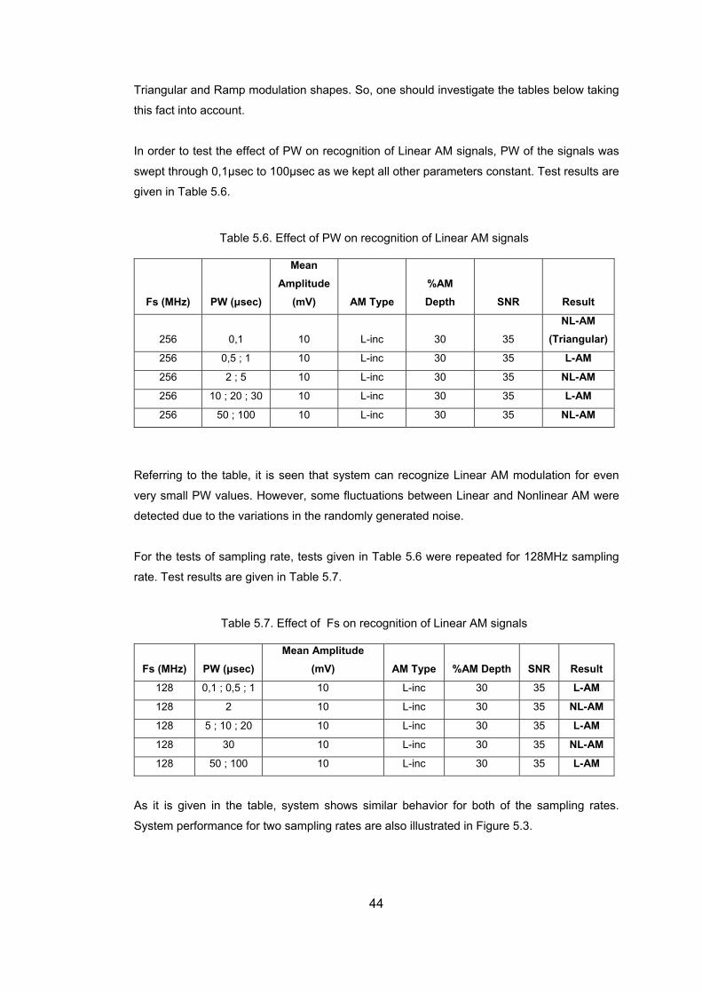
Triangular and Ramp modulation shapes. So, one should investigate the tables below taking
this fact into account.
In order to test the effect of PW on recognition of Linear AM signals, PW of the signals was
swept through 0,1µsec to 100µsec as we kept all other parameters constant. Test results are
given in Table 5.6.
Fs (MHz) PW (µsec)
Mean Amplitude
(mV) AM Type %AM Depth SNR Result
Table 5.6. Effect of PW on recognition of Linear AM signals
2
NL-AM ular) 56 0,1 10 L-inc 30 35 (Triang
256 0,5 ; 1 nc 30 35 L-AM 10 L-i
256 2 ; 5 10 L-inc N 30 35 L-AM
256 10 ; 20 ; 30 c 30 35 L-AM 10 L-in
256 50 ; 100 30 35 NL10 L-inc -AM
Referring to the table, it is seen that system can recognize Linear AM modulation for even
very small PW values. However, some fluctuations between Linear and Nonlinear AM were
etected due to the variations in the randomly generated noise.
pling
te. Test results are given in Table 5.7.
Table 5.7. Effect of Fs on recognition of Linear AM signals
Fs ) PW c) Mean tude
(mV) A e %AM pth SNR
d
For the tests of sampling rate, tests given in Table 5.6 were repeated for 128MHz sam
ra
(MHz (µse Ampli
M Typ De Result
128 0,1 ; 0,5 ; 1 10 L-inc 30 L-AM 35
128 2 10 L-inc 30 35 NL-AM
128 5 ; 10 ; 20 10 L-inc 30 35 L-AM
128 30 10 L-inc 30 35 NL-AM
128 50 ; 100 10 L-inc 30 35 L-AM
s iven in table, system shows similar ior for b of the mp s.
ystem performance for two sampling rates are also illustrated in Figure 5.3.
A it is g the behav oth sa ling rate
S
44
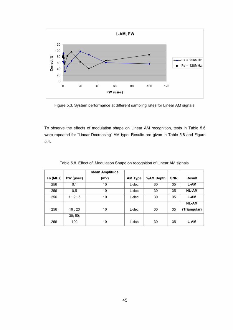
L-AM, PW
0
20
40
60
80
100
120
0 20 40 60 80 100 120
PW (usec)
Corr
ect % Fs = 256MHz
Fs = 128MHz
Figure 5.3. System performance at different sampling rates for Linear AM signals.
o observe the effects of modulation shape on Linear AM recognition, tests in Table 5.6
ere repeated for “Linear Decreasing” AM type. Results are given in Table 5.8 and Figure
5.4.
dulation Shape on recognition of Linear AM signals
Fs (M
T
w
Table 5.8. Effect of Mo
Hz) PW (µsec) Mean Amplitude
(mV) AM Type %AM Depth SNR Result
256 0,1 10 L-dec 30 35 L-AM
256 0,5 NL-AM 10 L-dec 30 35
256 1 ; 2 ; 5 10 L-dec 30 35 L-AM
256 10 ; 20 10 L-dec 30 35
NL-AM (Triangular)
256 100 10 L-dec 30 35 L-AM 30; 50;
45
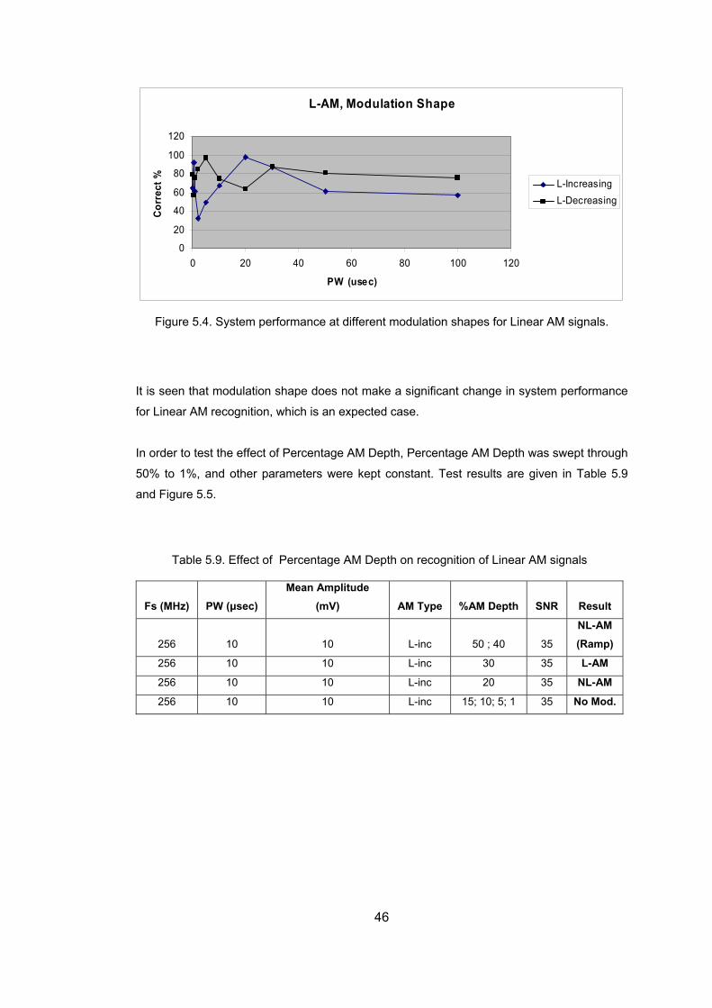
L-AM, M Sha
0
0
0
0 20 40 60 80 100 120
Corr
ect %
odulation pe
12
10
40
60
80L-IncreasingL-Decreasing
20
PW (usec)
Figure 5.4. System perf different modulati s for Linear AM signals.
It is se modulatio shape s no nificant change in system perfo ce
for L reco ion, whic n ex .
ord to test the effect of Percentage AM Depth, Percentage AM Depth was swept through
50%
and F
Fs (M sec) (mV) AM Type %AM Depth SNR Result
ormance at on shape
en that n doe t make a sig rman
inear AM gnit h is a pected case
In er
to 1%, and other parameters were kept constant. Test results are given in Table 5.9
igure 5.5.
Table 5.9. Effect of Percentage AM Depth on recognition of Linear AM signals
Hz) PW (µMean Amplitude
256 10 10 L-inc 50 ; 40 35
NL-AM (Ramp)
256 10 10 L-inc 30 35 L-AM
256 10 10 L-inc 20 35 NL-AM
256 10 10 L-inc 15; 10; 5; 1 35 No Mod.
46
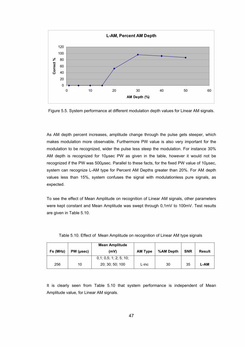
L-AM, Percent AM Depth
0
20
0 10 20 30 40 50
40
20
60
AM Depth (%)
Cor
rect
%
1
60
80
100
Figure 5.5. System perfo s.
As AM depth reas plitu e thr e pul stee ich
mak odulation more observable. Fu so very important for the
modulation to be gnized, w r the eep the modulation. For inst %
AM depth is reco for 10µsec PW in th ble, how
reco d if the PW was 500µ . Para facts, for the fixed PW value of 10µsec,
system can recognize L-AM type for Percent AM De r than 20%. For AM depth
alue ss than 15%, system confuse l with modulationless pure as
expected.
To see the effect of Mean Amplitude on recognition of Linear AM signals, other parameters
were kept constant and Mean Amplitude was swept through 0,1mV to 100mV. Test results
are given in Table 5.10.
Table 5.10. Effect of Mean Amplitude on recognition of Linear AM type signals
Fs (MHz) PW (µsec) Mean Amplitude
(mV) AM Type %AM Depth SNR Result
rmance at different modulation depth values for Linear AM signal
percent inc es, am de chang ough th se gets per, wh
es m rthermore PW value is al
reco ide pulse less st ance 30
gnized as given e ta ever it would not be
gnize sec llel to these
pths greate
v s le s the signa signals,
256 10
0,1; 0,5; 1; 2; 5; 10;
20; 30; 50; 100 L-inc 30 35 L-AM
It is early seen from Table 5.10 that system performance is independent of Mean
Amplitude value, for Linear AM signals.
cl
47
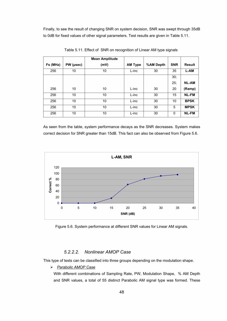
Finall
to 0dB
Table 5.11. Effect of SNR on recognition of Linear AM type signals
Fs (MHz)
y, to see the result of changing SNR on system decision, SNR was swept through 35dB
for fixed values of other signal parameters. Test results are given in Table 5.11.
PW (µsec) Mean Amplitude
(mV) AM Type %AM Depth SNR Result
25 35 L-AM 6 10 10 L-inc 30
25
30;
6 10 10 L-inc 30
25;
20
NL-AM (Ramp)
256 10 10 L-inc 30 15 NL-FM
256 10 10 L-inc 30 10 BPSK
25 SK 6 10 10 L-inc 30 5 MP
256 10 10 L-inc 30 0 NL-FM As the ta ance s as t R decr s. Syst kes
correct decision for SNR greater than 15dB. This fact can also be observed from Figure 5.6.
seen from ble, system perform decay he SN ease em ma
L-AM, SNR
0
20
40
60
80
100
120
0 5 10 15 20 25 30 35 40
S R (dB)
Cor
rect
%
N
Figure 5.6. System performance at different SNR values for Linear AM signals.
5.2.2.2. Nonlinear AMOP Case
This type of tests can be classified into three groups depending on the modulation shape.
Parabolic AMOP Case
With different combinations of Sampling Rate, PW, Modulation Shape, % AM Depth
and SNR values, a total of 55 distinct Parabolic AM signal type was formed. These
48
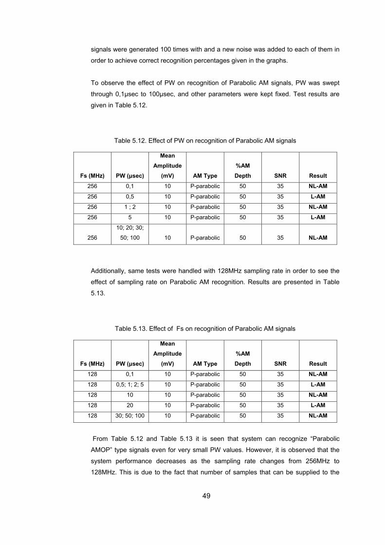
signals were generated 100 times with and a new noise was added to each of them in
order to achieve correct recognition percentages given in the graphs.
Table 5.12. Effect of PW on recognition of Parabolic AM signals
Am e %AM
To observe the effect of PW on recognition of Parabolic AM signals, PW was swept
through 0,1µsec to 100µsec, and other parameters were kept fixed. Test results are
given in Table 5.12.
Fs (MHz) PW (µsec)
Mean plitud(mV) AM Type Depth SNR Result
256 0,1 10 P-parabolic 50 35 NL-AM
256 0,5 P-parabolic 50 35 L-AM 10
256 1 ; 2 P-parabolic 50 35 NL-AM 10
256 5 10 P-parabolic 50 35 L-AM
256
10; 20; 30;
50; 100 10 P-parabolic 50 35 NL-AM
128MHz sampling rate in order to see the
ffect of sampling rate on Parabolic AM recognition. Results are presented in Table
Table 5.13. Effect of Fs on recognition of Parabolic AM signals
Fs (MHz) PW (µsec)
Amplitude
AM Type %AM Depth SNR Result
Additionally, same tests were handled with
e
5.13.
Mean
(mV)
128 0,1 P-parabolic 35 NL-AM 10 50
128 0,5; 1; 2; 5 10 P-parabolic 50 35 L-AM
128 10 10 P-parabolic 50 NL-AM 35
128 20 10 P-parabolic 50 35 L-AM
128 30; 50; 100 10 P-parabolic 50 35 NL-AM
ble d Ta that system can recognize “Pa c
MOP” type signals even for very small PW values. However, it is observed that the
ystem performance decreases as the sampling rate changes from 256MHz to
128MHz. This is due to the fact that number of samples that can be supplied to the
From Ta 5.12 an ble 5.13 it is seen raboli
A
s
49
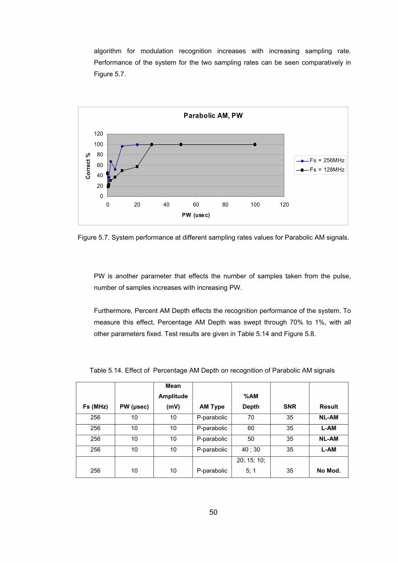
algorithm for modulation recognition increases with increasing sampling rate.
Performance of the system for the two sampling rates can be seen comparatively in
Figure 5.7.
Parabolic AM, PW
0
20
40
60
80
100
120
0 20 40 60 80 100 120
Corr
ect %
PW (usec)
Fs = 256MHzFs = 128MHz
Figure 5.7. System performance at different sampling rates values for Parabolic AM signals.
ercent AM Depth effects the recognition performance of the system. To
easure this effect, Percentage AM Depth was swept through 70% to 1%, with all
T t of Percentage AM Depth on recognition of Parabolic AM signals
Fs (MHz)
Mean Amplitude %AM
Result
PW is another parameter that effects the number of samples taken from the pulse,
number of samples increases with increasing PW.
Furthermore, P
m
other parameters fixed. Test results are given in Table 5.14 and Figure 5.8.
able 5.14. Effec
PW (µsec) (mV) AM Type Depth SNR
256 10 10 P-parabolic 70 35 NL-AM
256 0 P-parabo 35 L-AM 1 10 lic 60
256 10 10 ab 35 NP-par olic 50 L-AM
256 10 aboli 40 ; 30 35 10 P-par c L-AM
256 10 10 P-parabolic
20; 15; 1
5; 1 35 No Mod. 0;
50
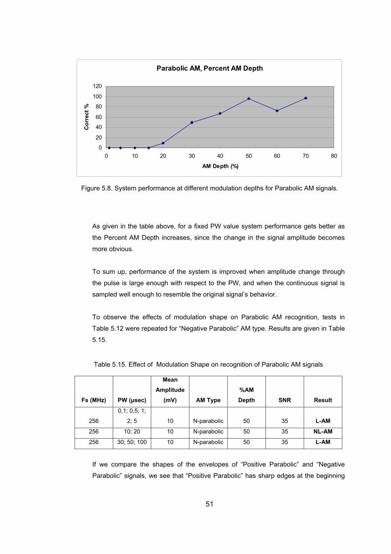
Parabolic AM, Percent AM Depth
0
20
40
1
60
80
100
20
0 70 80
AM Depth (%)
Cor
rect
%
10 20 30 40 50 60
8. per ce m n ara AM
given he table ove, PW lue system performance gets as
the Pe Depth increases, since the change in the signal amplitude becomes
re obvious.
o sum up, performance of the system is improved when amplitude change through
the pulse is large enough with respect to the PW, and when the continuous signal is
sampled well enough to resemble the original signal’s behavior.
To observe the effects of modulation shape on Parabolic AM recognition, tests in
Table 5.12 were repeated for “Negative Parabolic” AM type. Results are given in Table
5.15.
Table 5.15. Effect of Modulation Shape on recognition of Parabolic AM signals
Fs (MHz) PW (µsec)
Mean Amplitude
(mV) AM Type %AM Depth SNR Result
Figure 5. System forman at different odulatio depths for P bolic signals.
As in t ab for a fixed va better
rcent AM
mo
T
256 2; 5 10 N-parabolic 50 35 L-AM 0,1; 0,5; 1;
256 10; 20 10 N-parabolic 50 35 NL-AM
256 30; 50; 100 10 N-parabolic 50 35 L-AM
If we compare the shapes of the envelopes of “Positive Parabolic” and “Negative
Parabolic” signals, we see that “Positive Parabolic” has sharp edges at the beginning
51
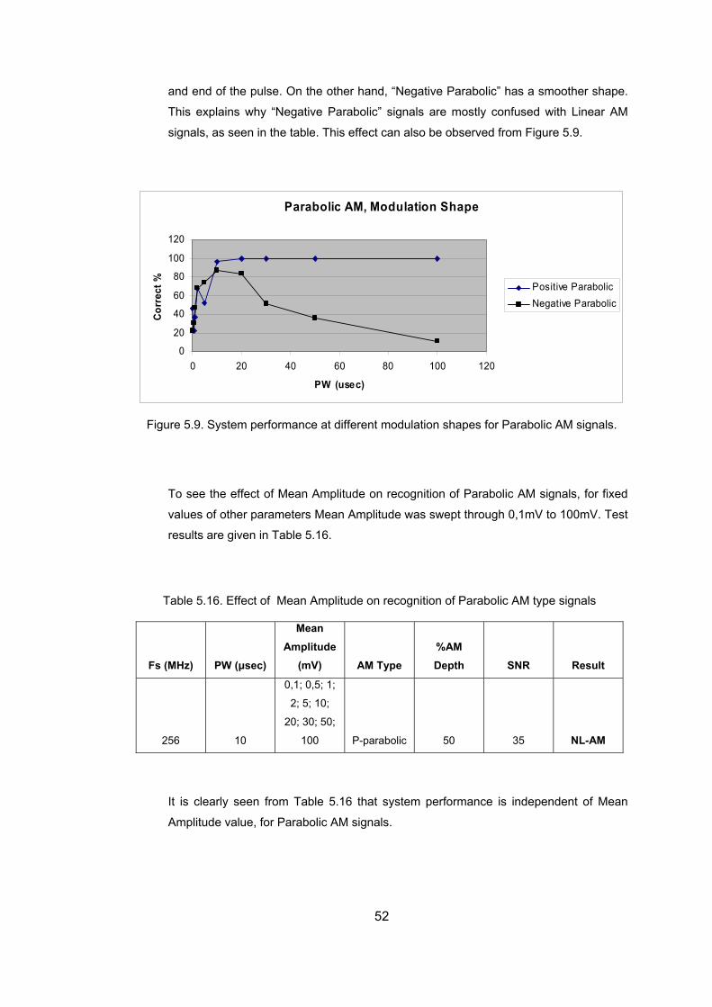
and end of the pulse. On the other hand, “Negative Parabolic” has a smoother shape.
This explains why “Negative Parabolic” signals are mostly confused with Linear AM
ignals, as seen in the table. This effect can also be observed from Figure 5.9. s
Parabolic AM, Modulation Shape
0
20
C 40
60
80
0
0 20 80 100 20
P
orre
ct %
100
12
40 60 1
W (usec)
Positive ParabolicNegative Parabolic
Figure 5.9. System perfo nce m n sha for Para AM
Table 5.16. Effect of Mean Amplitude on recognition of Parabolic AM type signals
Fs (MHz) PW (µsec)
Mean Amplitude
(mV) AM Type %AM Depth SNR Result
rma at different odulatio pes bolic signals.
To see the effect of Mean Amplitude on recognition of Parabolic AM signals, for fixed
values of other parameters Mean Amplitude was swept through 0,1mV to 100mV. Test
results are given in Table 5.16.
256 10
0,1; 0,5; 1;
2; 5; 10;
20; 30; 50;
100 P-parabolic 50 35 NL-AM
It is clearly seen from Table 5.16 that system performance is independent of Mean
Amplitude value, for Parabolic AM signals.
52
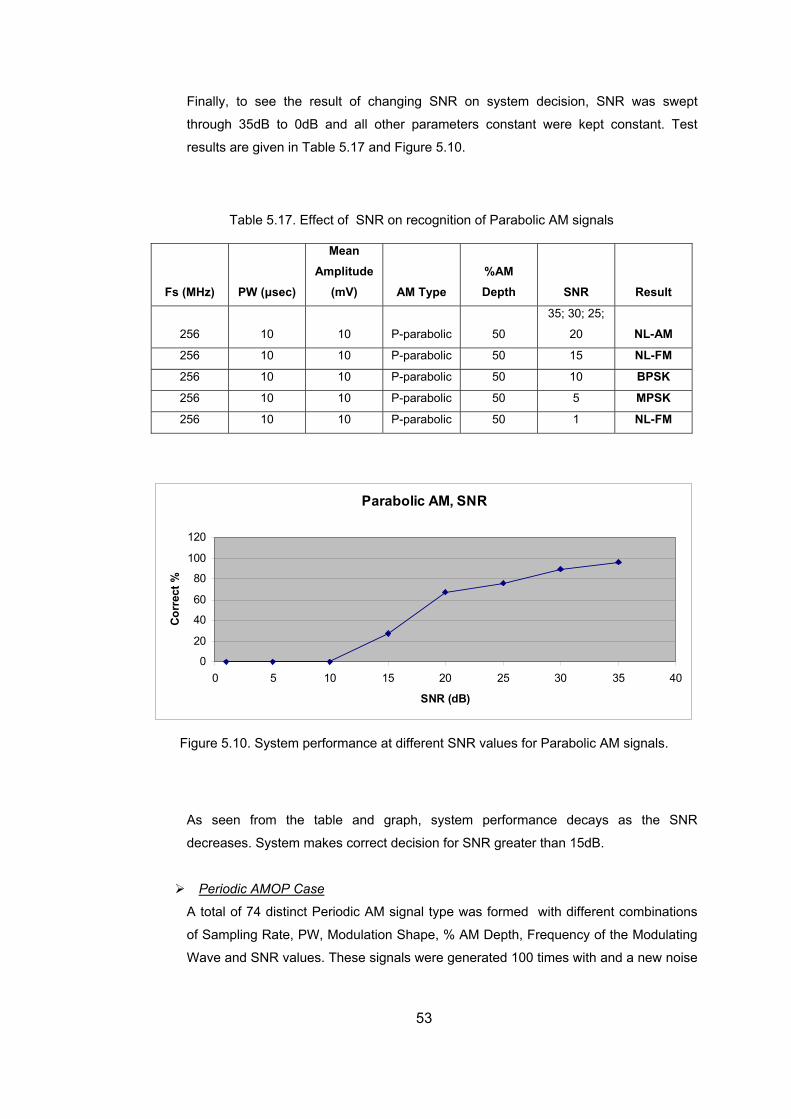
Finally, to see the result of changing SNR on system decision, SNR was swept
rough 35dB to 0dB and all other parameters constant were kept constant. Test
Table 5.17. Effect of SNR on recognition of Parabolic AM signals
Fs ( (mV) AM Type Depth SNR Result
th
results are given in Table 5.17 and Figure 5.10.
MHz) PW (µsec)
Mean Amplitude %AM
256 10 10 P-parabolic 50
35; 30; 25;
20 NL-AM
25 M 6 10 10 P-parabolic 50 15 NL-F
256 10 10 P-parabolic 50 10 BPSK
256 10 10 P-parabolic 50 5 MPSK
256 10 10 P-parabol 1 NL-FM ic 50
Parabolic AM NR
0
40
60
80
100
0
0 5 0 2 25 30 35
SNR (d
Corr
ect %
, S
20
12
1 15 0 40
B)
ure 5.1 ystem p rmance at different R values for Parabolic AM sign
As se the table and graph, system performance decays as the SNR
creas ystem m es corr is n NR gr an 15
Periodic AMOP Case
Fig 0. S erfo SN als.
en from
es. Sde ak ect dec io for S eater th dB.
A total of 74 distinct Periodic AM signal type was formed with different combinations
of Sampling Rate, PW, Modulation Shape, % AM Depth, Frequency of the Modulating
Wave and SNR values. These signals were generated 100 times with and a new noise
53
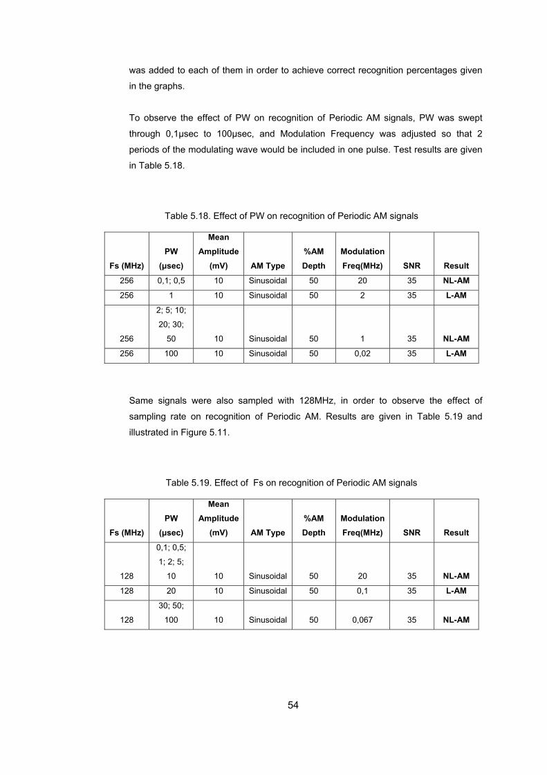
was added to each of them in order to achieve correct recognition percentages given
in the graphs.
To observe the effect of PW on recognition of Periodic AM signals, PW was swept
through 0,1µsec to 100µsec, and Modulation Frequency was adjusted so that 2
eriods of the modulating wave would be included in one pulse. Test results are given
Table 5.18.
Table 5.18. Effect of PW on recognition of Periodic AM signals
Fs (MHz) PW
(µsec)
Mean Amplitude
(mV) AM Type %AM Depth
Modulation Freq(MHz) SNR Result
p
in
256 0,1; 0,5 10 Sinusoidal 50 20 35 NL-AM
256 1 10 Sinusoidal 50 2 35 L-AM
256
2; 5; 10;
20; 30;
50 10 Sinusoidal 50 1 35 NL-AM
256 100 10 Sinusoidal 50 0,02 35 L-AM
ame signals were also sampled with 128MHz, in order to observe the effect of
Table 5.19. Effect of Fs on recognition of Periodic AM signals
Fs (MHz) PW
(µsec)
Mean Am e
AM Type %AM Modulation
SNR Result
S
sampling rate on recognition of Periodic AM. Results are given in Table 5.19 and
illustrated in Figure 5.11.
plitud(mV) Depth Freq(MHz)
128
1; 2; 5;
10 10 Sinusoidal 50 20 35 NL-AM
0,1; 0,5;
128 20 Sinusoidal 50 0,1 35 L-AM 10
128
30; 50;
100 10 Sinusoidal 50 0,067 35 NL-AM
54
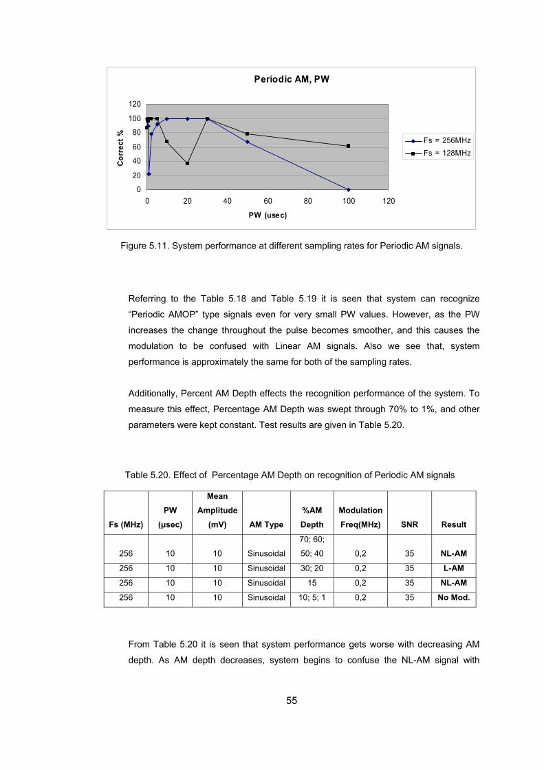
Periodic AM, PW
100
120
0
20
40
0 20 60 20
Corr
ect %
80
60
40 80 100 1
PW (usec)
Fs = 256MHzFs = 128MHz
re 5.11 stem p ent pling rat r Peri si
g to the Table 5.18 and T e 5.19 it is see hat syste can
eriodic AMOP” type signals even for very small PW values. However, as the PW
creases the change throughout the pulse becomes smoother, and this causes the
dditionally, Percent AM Depth effects the recognition performance of the system. To
easure this effect, Percentage AM Depth was swept through 70% to 1%, and other
parameters were kept constant. Test results are given in Table 5.20.
Table 5.20. Effect of Percentage AM Depth on recognition of Periodic AM signals
Fs (MHz) PW
(µsec)
Mean Amplitude
(mV) AM Type %AM Depth
Modulation Freq(MHz) SNR Result
Figu . Sy erformance at differ sam es fo odic AM gnals.
Referrin abl n t m recognize
“P
in
modulation to be confused with Linear AM signals. Also we see that, system
performance is approximately the same for both of the sampling rates.
A
m
256 10 10 Sinusoidal
70; 60;
50; 40 0,2 35 NL-AM
256 10 10 Sinusoidal 30; 20 0,2 35 L-AM
256 10 10 Sinusoidal 15 0,2 35 NL-AM
256 10 10 Sinusoidal 10; 5; 1 0,2 35 No Mod.
From Table 5.20 it is seen that system performance gets worse with decreasing AM
depth. As AM depth decreases, system begins to confuse the NL-AM signal with
55
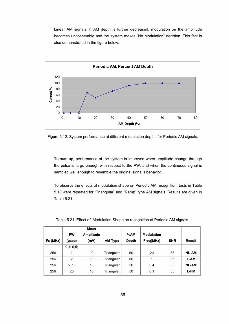
Linear AM signals. If AM depth is further decreased, modulation on the amplitude
becomes unobservable and the system makes “No Modulation” decision. This fact is
also demonstrated in the figure below.
Periodic AM, Percent AM Depth
0
20
40
60
100
120
0 10 0 4 70
De (%)
Cor
re
80
ct %
2 30 0 50 60 80
AM pth
Figure 5.12. System performance at different modulation depths for Periodic AM signals.
the pulse is large enough with resp PW, and when the continuous signal is
ampled well enough to resemble the original signal’s behavior.
t of Modulation Shape on recognition of Periodic AM signals
Fs (M
To sum up, performance of the system is improved when amplitude change through
ect to the
s
To observe the effects of modulation shape on Periodic AM recognition, tests in Table
5.18 were repeated for “Triangular” and “Ramp” type AM signals. Results are given in
Table 5.21.
Table 5.21. Effec
Mean
Hz) PW
(µsec) Amplitude
(mV) AM Type %AM Depth
Modulation Freq(MHz) SNR Result
256
0,1; 0,5;
1 10 Triangular 50 20 35 NL-AM
256 2 10 Triangular 50 1 35 L-AM
25 gular 50 0,4 35 NL-AM 6 5; 10 10 Trian
256 20 10 Triangular 50 0,1 35 L-FM
56
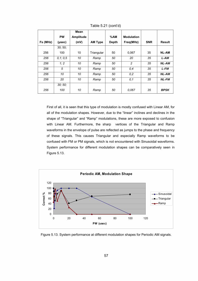
Table 5.21 (cont’d)
Hz) PW
(µsec)
Mean Amplitude %AM Modulation
Fs (M (mV) AM Type Depth Freq(MHz) SNR Result
256
30; 50;
100 10 Triangular 50 0,067 35 NL-AM
256 0,1; 0,5 10 Ramp 50 20 35 L-AM
256 1; 2 10 Ramp 50 2 35 NL-AM
256 5 10 Ramp 50 0,4 35 L-FM
256 10 10 Ramp 50 0,2 35 NL-AM
256 NL-FM 20 10 Ramp 50 0,1 35
256
30; 50;
35 BPSK 100 10 Ramp 50 0,067
st of a is seen that this type of modulation is mostly confused with Linea for
all of th lation shapes. However, due to the “linear” inclines and declines in the
shape gular” and “Ramp” modulations, these are more exposed to confusion
th Li M. Fu rmore, sharp ertices Tria lar a p
veform the en pe of pu are reflected as jumps to the phase and cy
f these signals. This causes Triangular and especially Ramp waveforms to be
onfused with FM or PM signals, which is not encountered with Sinusoidal waveforms.
Fir ll, it r AM,
e modu
of “Trian
near Awi rthe the v of the ngu nd Ram
wa s in velo lse frequen
o
c
System performance for different modulation shapes can be comparatively seen in
Figure 5.13.
Periodic AM, Modulation Shape
0
20
40
0
0
120
0 0 40 60 80 100 120
P sec)
Corr
ect %
100
8 SinusoidalTriangular6
2
W (u
Ramp
Figure 5.13. System performance at different modulation shapes for Periodic AM signals.
57
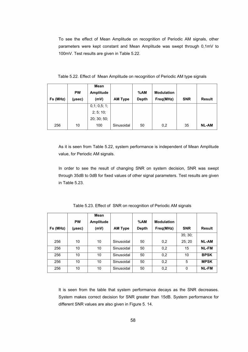
To see the effect of Mean Amplitude on recognition of Periodic AM signals, other
parameters were kept constant and Mean Amplitude was swept through 0,1mV to
100mV. Test results are given in Table 5.22.
Table 5.22. Effect of Mean Amplitude on recognition of Periodic AM type signals
PW Mean
Amplitude %AM Modulation Fs (MHz) (µsec) (mV) AM Type Depth Freq(MHz) SNR Result
256 10
0,1; 0,5; 1;
2; 5; 10;
20; 30; 50;
100 Sinusoidal 50 0,2 35 NL-AM
As it is seen from Table 5.22, system performance is independent of Mean Amplitude
value, for Periodic AM signals.
In order to see the result of changing SNR on system decision, SNR was swept
through 35dB to 0dB for fixed values of other signal parameters. Test results are given
in Table 5.23.
Table 5.23. Effect of SNR on recognition of Periodic AM signals
Fs (M
Hz) PW
(µsec)
Mean Amplitude
(mV) AM Type %AM Depth
Modulation Freq(MHz) SNR Result
256 10 10 Sinusoidal 50 0,2
35; 30;
25; 20 NL-AM
256 10 10 Sinusoidal 50 0,2 15 NL-FM
256 10 10 Sinusoidal 50 0,2 10 BPSK
2 K 56 10 10 Sinusoidal 50 0,2 5 MPS
256 10 Sinusoidal 50 0,2 0 NL-FM 10
It is seen from the table that system p nce decays as the SNR decreases.
stem m es corre ecision SNR g er than 15dB. System perform for
ferent values also given in Figure 5. 14.
erforma
reatSy ak ct d for ance
dif SNR are
58
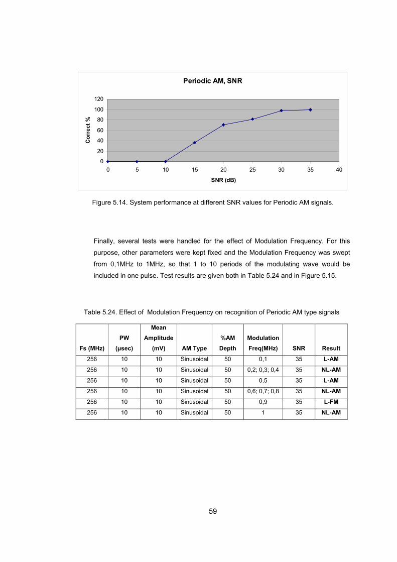
Periodic AM R
0
20
40
80
00
Co
t %, SN
120
1
60rrec
0 5 10 15 20 25 30 35 40
SNR (dB)
Figure 5.14. System performance at different SNR values for Periodic AM signals.
Finally, several tests were handled for the effect of Modulation Frequency. For this
urpose, other parameters were kept fixed and the Modulation Frequency was swept
Ta Frequency on recognition of Periodic AM type signals
Fs (MHz) PW
Mean Amplitude %AM Modulation
Result
p
from 0,1MHz to 1MHz, so that 1 to 10 periods of the modulating wave would be
included in one pulse. Test results are given both in Table 5.24 and in Figure 5.15.
ble 5.24. Effect of Modulation
(µsec) (mV) AM Type Depth Freq(MHz) SNR
256 10 Sinusoidal 50 0,1 35 L-AM 10
256 Si al 35 NL-AM 10 10 nusoid 50 0,2; 0,3; 0,4
256 10 10 Si l nusoida 50 0,5 35 L-AM
256 10 10 Sinu idal 0,6; 0,7; 0,8 so 50 35 NL-AM
256 10 10 Sin dal usoi 50 0,9 35 L-FM
256 10 10 S inusoidal 50 1 35 NL-AM
59
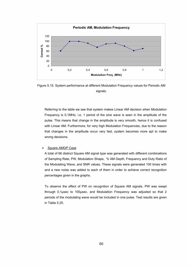
Periodic AM, Modulation Frequency
0
20
40
60
80
100
120
0 0,2 0,4 0,6 0,8 1 1,2
Modulation Freq. (MHz)
Cor
rect
%
Fig M
signals.
cision when Modulation
requency is 0,1MHz, i.e. 1 period of the sine wave is seen in the amplitude of the
occur very fast, system becomes more apt to make
rong decisions.
ure 5.15. System performance at different Modulation Frequency values for Periodic A
Referring to the table we see that system makes Linear AM de
F
pulse. This means that change in the amplitude is very smooth, hence it is confused
with Linear AM. Furthermore, for very high Modulation Frequencies, due to the reason
that changes in the amplitude
w
Square AMOP Case
A total of 66 distinct Square AM signal type was generated with different combinations
of Sampling Rate, PW, M pe, % AM Depth, Fre ncy and Duty Ratio of
o Wave, and SNR s. T ign rated 100 th
and a new noise d to each of them in order to achieve correct recognition
percentages given aphs.
obse he effe PW o cognition of Squar signals, PW w pt
rough 0,1µsec to 100µsec, and Modulation Frequency was adjusted so that 2
eriods of the modulating wave would be included in one pulse. Test results are given
odulation Sha
value
que
als were genethe M dulating hese s times wi
was adde
in the gr
ct ofTo rve t n re e AM as swe
th
p
in Table 5.25.
60
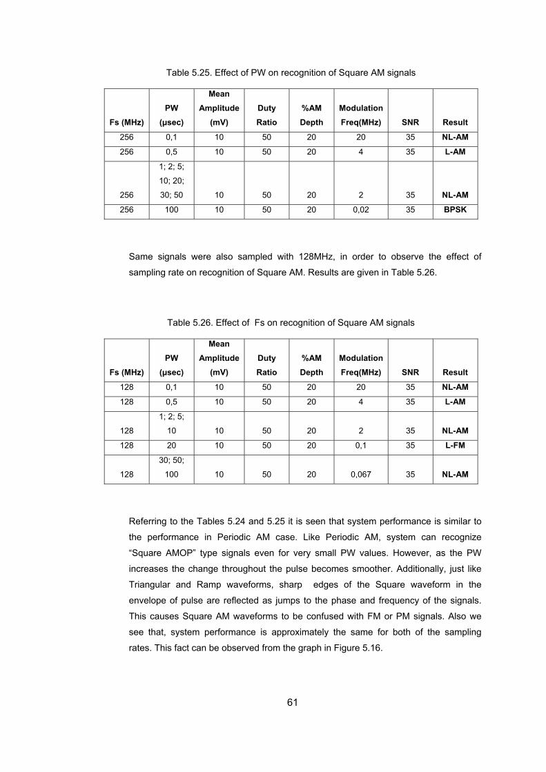
Table 5.25. Effect of PW on recognition of Square AM signals
Fs (MHz) (µsec)
Mean
Ratio Depth Freq(MHz) SNR Result PW Amplitude Duty %AM Modulation
(mV)
256 35 NL-AM 0,1 10 50 20 20
256 0,5 10 50 20 4 35 L-AM
256
1; 2; 5;
10; 20;
30; 50 10 50 20 2 35 NL-AM
256 100 10 50 20 0,02 35 BPSK
ame signals were also sampled with 128MHz, in order to observe the effect of
Table 5.26. Effect of Fs on recognition of Square AM signals
Fs (MPW
Mean Amplitude Duty %AM Modulation
lt
S
sampling rate on recognition of Square AM. Results are given in Table 5.26.
Hz) (µsec) (mV) Ratio Depth Freq(MHz) SNR Resu
128 0,1 10 50 20 20 35 NL-AM
128 0,5 10 50 20 4 35 L-AM
12
1; 2; 5;
8 10 10 50 20 2 35 NL-AM
128 20 10 50 20 0,1 35 L-FM
128
30; 50;
100 10 50 20 0,067 35 NL-AM
to
the performance in Periodic AM case. Like Periodic AM, system can recognize
“Square AMOP” ty nals even for very small PW values. However, as the PW
se pulse r. Additionally, ke
Triangular and Ramp waveforms, sharp edges of the Square waveform in the
velope pulse a flected jumps to the pha frequency of the signals.
is cau Square AM waveforms to be fused with FM or PM signals. we
e that tem pe mance i pproxim ly th both of the g
tes. Th ct can b served from the gr in Figu .
Referring to the Tables 5.24 and 5.25 it is seen that system performance is similar
pe sig
ange throughoincrea s the ch ut the becomes smoothe just li
en of re re as se and
Th ses con Also
se , sys rfor s a ate e same for samplin
ra is fa e ob aph re 5.16
61
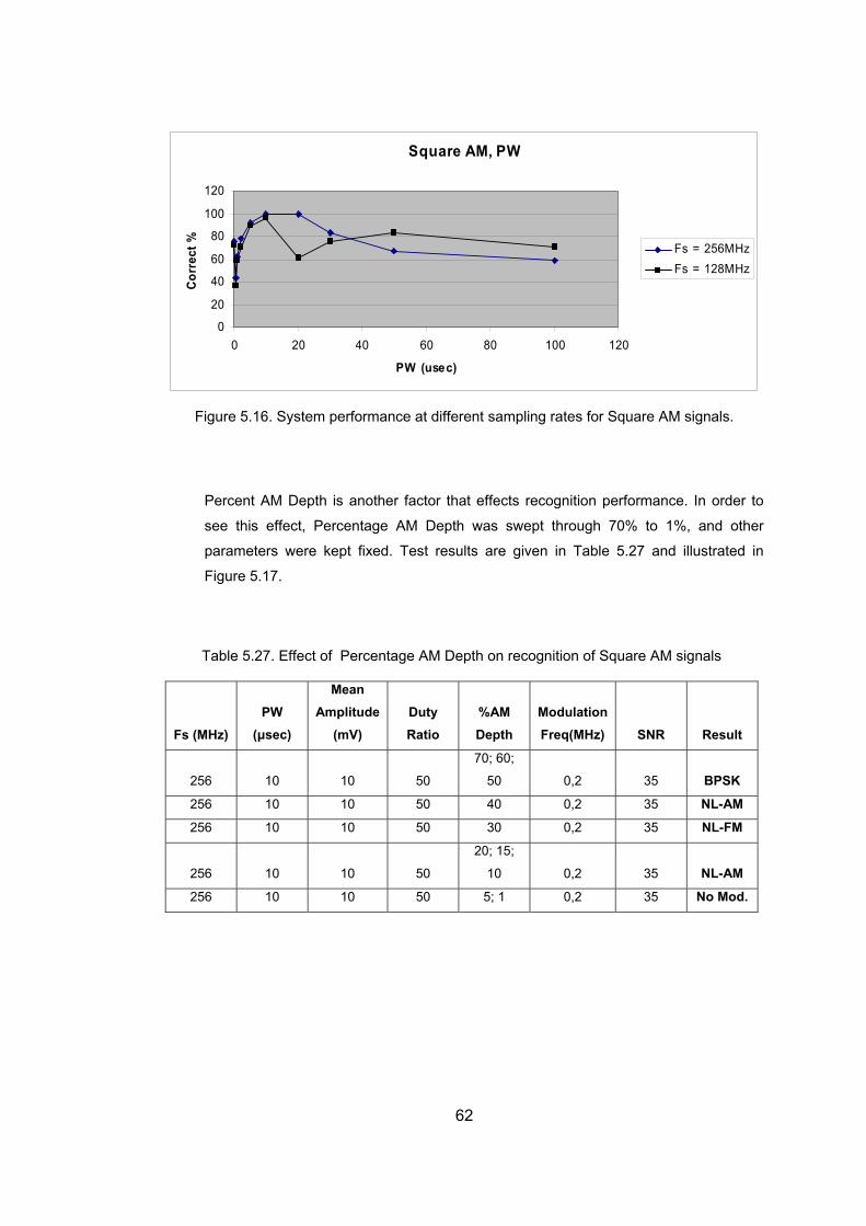
Square AM, PW
0
20
40
60
80
100
120
0 20 40 60 80 100 120
PW (usec)
Corr
ect % Fs = 256MHz
Fs = 128MHz
Figure 5.16. System performance at different sampling rates for Square AM signals.
Percent AM Depth is another factor that effects recognition performance. In order to
see this effect, Percentage AM Depth was swept through 70% to 1%, and other
parameters were kept fixed. Test results are given in Table 5.27 and illustrated in
Figure 5.17.
Table cognition of Square AM signals 5.27. Effect of Percentage AM Depth on re
Fs (MHz) PW
(µsec)
Mean Amplitude
(mV) Duty Ratio
%AM Depth
Modulation Freq(MHz) SNR Result
256 10 10 50 50 0,2 35 BPSK 70; 60;
256 10 10 50 40 0,2 35 NL-AM
256 10 10 50 30 0,2 35 NL-FM
256 10 10 50
20; 15;
10 0,2 35 NL-AM
256 10 10 50 5; 1 0,2 35 No Mod.
62
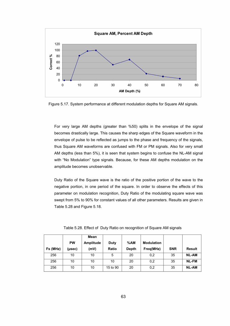
Square AM, Percent AM Depth
0
20
40
60
80
100
120
0 3 40 0 60 70 010 20 0 5 8
AM Depth (%)
Cor
rect
%
Figure 5.17. System performance at different modulation depths for Square AM signals.
nvelope of the signal
becomes drastically large. This causes the sharp edges of the Square waveform in the
begins to confuse the NL-AM signal
with “No Modulation” type signals. Because, for these AM depths modulation on the
amplitude becomes unobservable.
Duty Ratio of the Square wave is the ratio of the positive portion of the wave to the
negative portion, in one period of the square. In order to observe the effects of this
parameter on modulation recognition, Duty Ratio of the modulating square wave was
swept from 5% to 90% for constant values of all other parameters. Results are given in
Table 5.28 and Figure 5.18.
Table 5.28. Effect of Duty Ratio on recognition of Square AM signals
Fs (MHz) (µsec)
MeAmplitude
(mVDuRa
%AM Depth
odulation req(MHz) NR
For very large AM depths (greater than %50) splits in the e
envelope of pulse to be reflected as jumps to the phase and frequency of the signals,
thus Square AM waveforms are confused with FM or PM signals. Also for very small
AM depths (less than 5%), it is seen that system
PW an
) ty tio
MF S Result
256 10 10 5 20 0,2 35 NL-AM
256 10 10 10 20 0,2 35 NL-FM
256 10 10 15 to 20 0,2 35 90 NL-AM
63
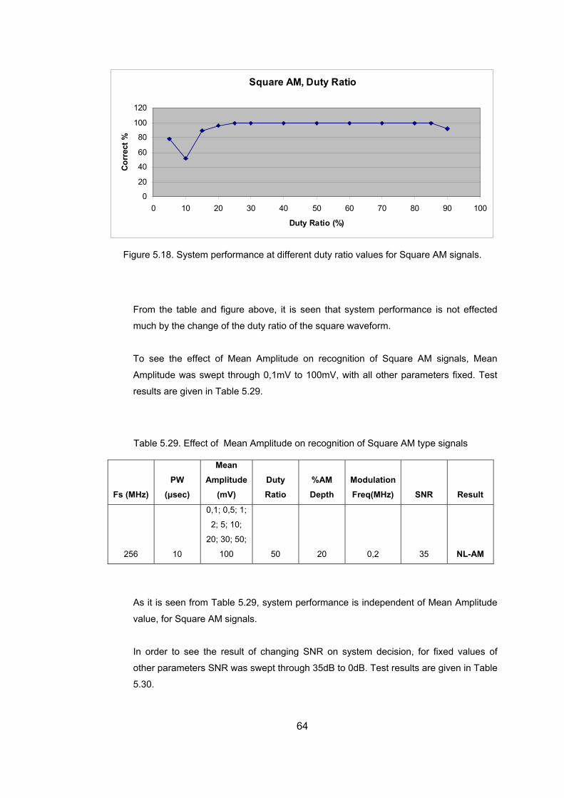
Square AM, Duty Ratio
40
60
80
120
Cor
rect
%100
0
20
0 10 20 30 40 50 60 70 80 90 100
Duty Ratio (%)
From the table and figure above, it is seen that system performance is not effected
much by the change of the duty ratio of the square waveform.
T
Amplitude was swept through 0,1mV to 100mV, with all other parameters fixed. Test
results are given in Ta 9.
ble 5.29. recognition of Square AM type sign
Fs (MHz) PW
(µ
MeaAmplitude
(mVDuRa
%AM Depth
odulation req(MHz) NR
Figure 5.18. System performance at different duty ratio values for Square AM signals.
o see the effect of Mean Amplitude on recognition of Square AM signals, Mean
ble 5.2
Ta Effect of Mean Amplitude on als
sec)
n
) ty tio
MF S Result
256 10
0,1; 0,5; 1;
2; 5;
20; 30; 50;
100 50 20 0,2 35 NL-AM
10;
As it is seen from Table 5.29, system performance is independent of Mean Amplitude
value, for Square AM signals.
In order to see the result of changing SNR on system decision, for fixed values of
other parameters SNR was swept through 35dB to 0dB. Test results are given in Table
5.30.
64
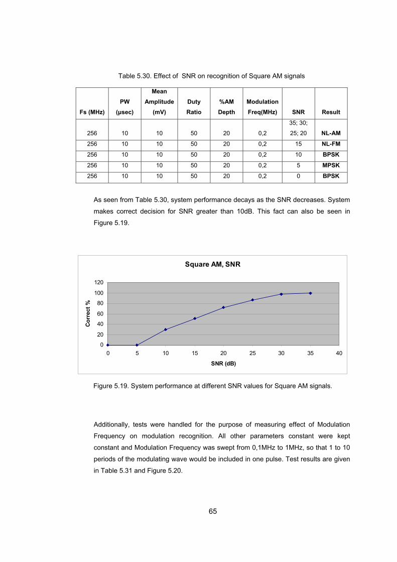
Table 5.30. Effect of SNR on recognition of Square AM signals
Fs (MHz) PW
(µsec)
Mean Amplitude
(mV) Duty Ratio
%AM Depth
Modulation Freq(MHz) SNR Result
256 10 10 50 20 0,2
35; 30;
25; 20 NL-AM
256 10 10 50 20 0,2 15 NL-FM
256 10 10 50 20 0,2 10 BPSK
256 10 10 50 20 0,2 5 MPSK
256 10 10 50 20 0,2 0 BPSK
As seen from Table 5.30, system performance decays as the SNR decreases. System
makes correct decision for SNR greater than 10dB. This fact can also be seen in
Figure 5.19.
Square AM, SNR
0
20
40
60
100
120
0 5 15 20 30 35
SNR (dB)
Cor
rect
% 80
10 25 40
ure 5.19 stem pe mance at different SN s for Squ AM si
Additionally, tests were handled for the purpose of measuring effect of Modulation
pt
constant and Modulation Frequency pt from 0,1MHz to 1MHz, so that 1 to 10
periods of the modulating wave would be included in one pulse. Test results are given
in Table 5.31 and Figure 5.20.
Fig . Sy rfor R value are gnals.
Frequency on modulation recognition. All other parameters constant were ke
was swe
65
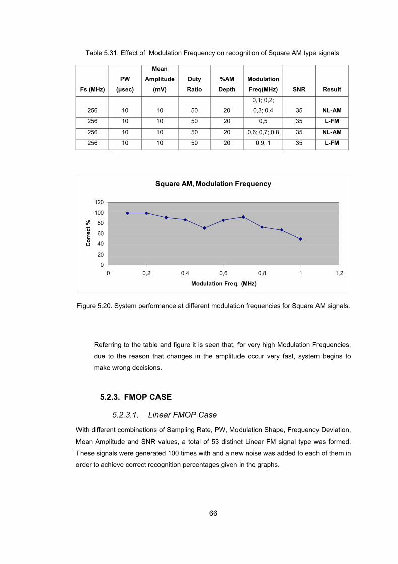
Table 5.31. Effect of Modulation Frequency on recognition of Square AM type signals
Fs (MHz) PW
(µsec)
Mean Amplitude
(mV) Duty Ratio
%AM Depth
Modulation Freq(MHz) SNR Result
256 10 10 50
0,1; 0,2;
20 0,3; 0,4 35 NL-AM
256 10 10 50 20 0,5 35 L-FM
256 10 10 50 20 0,6; 0,7; 0,8 35 NL-AM
256 10 10 50 20 0,9; 1 35 L-FM
Square AM, Modulation Frequency
0
20
40
60
80
100
120
0 0,2 0,4 0,6 0,8 1 1,2
Modulation Freq. (MHz)
Cor
rect
%
gins to
make wrong decisions.
5.2.3. FMOP CASE
5.2.3.1. Linear FMOP Case
With different s of Sampling n Shape, Fre cy Deviation,
Mea plitude SNR va s, a tot distinct ear FM si pe wa ed.
These signals were generated 100 times with and a new noise was added to each in
orde chieve correct recognition percentages given in the graphs.
Figure 5.20. System performance at different modulation frequencies for Square AM signals.
Referring to the table and figure it is seen that, for very high Modulation Frequencies,
due to the reason that changes in the amplitude occur very fast, system be
combination Rate, PW, Modulatio quen
gnal tyn Am and lue al of 53 Lin s form
of them
r to a
66
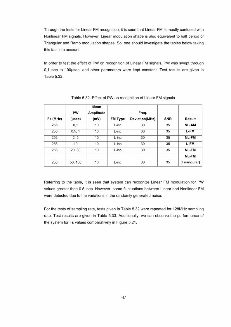
Through the tests for Linear FM recognition, it is seen that Linear FM is mostly confused with
king
is fact into account.
In order to test the effect of PW on recognition of Linear FM signals, PW was swept through
0,1µsec to 100µsec, and other parameters were kept constant. Test results are given in
Table 5.32.
Table 5.32. Effect of PW on recognition of Linear FM signals
Fs (MHz) PW
(µsec)
Mean Amplitude
(mV) FM Type Freq.
Deviation(MHz) SNR Result
Nonlinear FM signals. However, Linear modulation shape is also equivalent to half period of
Triangular and Ramp modulation shapes. So, one should investigate the tables below ta
th
256 0,1 10 L-inc 30 35 NL-AM
256 0,5; 1 10 L-inc 30 35 L-FM
25 6 2; 5 10 L-inc 30 35 NL-FM
256 10 10 L-inc 30 35 L-FM
256 20; 30 10 L-inc 30 35 NL-FM
256 50; 100 10 L-inc 30 35 (TriangularNL-FM
)
Referrin em can recognize Linear FM modulation for PW
values greate
were dete
For the test sampling
rate. Test results are given in Table 5.33. Additionally, we can observe the performance of
the system fo
g to the table, it is seen that syst
r than 0.5µsec. However, some fluctuations between Linear and Nonlinear FM
cted due to the variations in the randomly generated noise.
s of sampling rate, tests given in Table 5.32 were repeated for 128MHz
r Fs values comparatively in Figure 5.21.
67
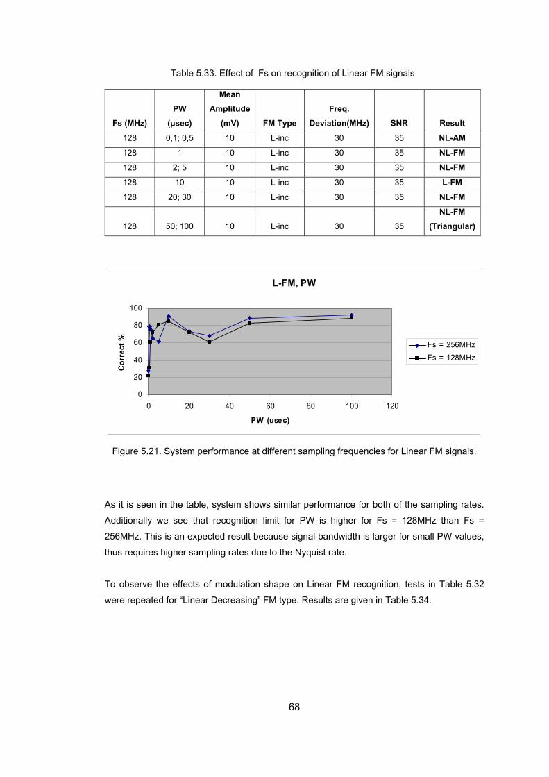
Table 5.33. Effect of Fs on recognition of Linear FM signals
Fs (MHz) PW
(µsec)
Mean Amplitude
(mV) FM Type Freq.
Deviation(MHz) SNR Result
128 0,1; 0,5 10 L-inc 30 35 NL-AM
128 NL-FM 1 10 L-inc 30 35
128 2; 5 L-inc 30 35 NL-FM 10
128 10 L-inc 35 L-FM 10 30
128 20; 30 10 L-inc 30 35 NL-FM
128 50 30 35
NL-FM (Tr ) ; 100 10 L-inc iangular
L-FM, PW
0
20
40
60
80
100
0
PW (usec)
Cor
rect
% Fs = 256MHz
20 40 60 80 100 120
Fs = 128MHz
1 rfor at d m s for Linear FM
As it is seen , system shows s ilar performance for both of the sampling rates.
dd lly we that recognition li W is h r for Fs = 128MHz =
z. This is an expected result because signal bandwidth is larger for small PW values,
thus r res higher sampling rates due to the Nyquist rate.
To 32
were repeated for “Linear Decreasing” FM type. Results are given in Table 5.34.
Figure 5.2 . System pe mance ifferent sa pling frequencie signals.
in the table
see
im
mit for PA
256M
itiona ighe than Fs
H
equi
observe the effects of modulation shape on Linear FM recognition, tests in Table 5.
68
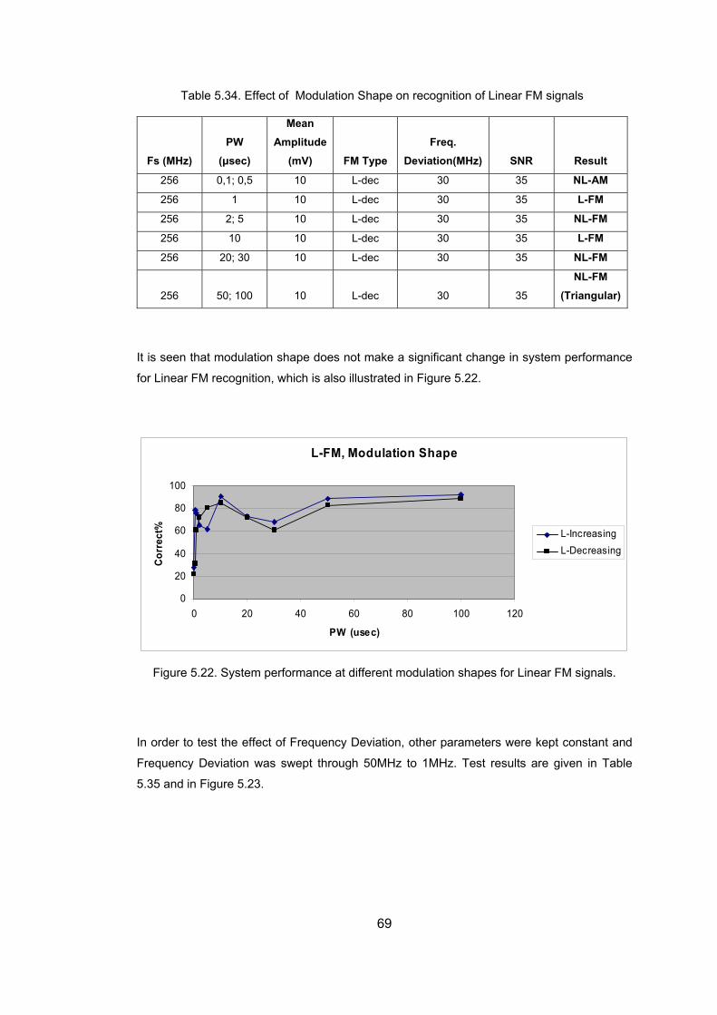
Table 5.34. Effect of Modulation Shape on recognition of Linear FM signals
Fs (MHz) PW
(µsec)
Mean Amplitude
(mV) FM Type Freq.
Deviation(MHz) SNR Result
2 L-dec 30 35 NL-AM 56 0,1; 0,5 10
256 1 10 L-dec 30 35 L-FM
256 2; 5 10 L-dec 30 35 NL-FM
256 10 10 L-dec 30 35 L-FM
256 20; 30 10 L-dec 30 35 NL-FM
256 50; 100 L-dec 35
NL-FM (Triangular) 10 30
It is seen that modulation shape does not make a significant change in system performance
for Linear FM recognition, whi s also in Figu .22.
ch i illustrated re 5
L-FM, Modulation Sh
0
PW (usec)
Corr
ect%
ape
10
80
0
20
40
60
0 20 40 60 80 100 120
L-IncreasingL-Decreasing
Figure 5.22. System performance at different modulation shapes for Linear FM signals.
In order to test the effect of Frequency Deviation, other parameters were kept constant and
Frequency Deviation was swept through 50MHz to 1MHz. Test results are given in Table
5.35 and in Figure 5.23.
69
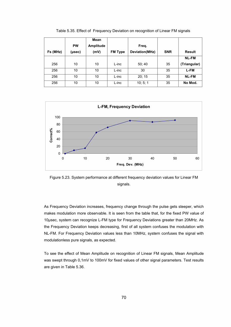
Table 5.35. Effect of Frequency Deviation on recognition of Linear FM signals
Fs (MHz) PW
(µsec)
Mean Amplitude
(mV) FM Type Freq.
Deviation(MHz) SNR Result
256 10 10 L-inc 50; 40 35
NL-FM (Triangular)
256 10 10 L-inc 30 35 L-FM
256 10 10 L-inc 20; 15 35 NL-FM
256 10 10 L-inc 10; 5; 1 35 No Mod.
L-FM, Frequency Deviation
0
20
40
60
80
0 10 20 30 40 0 6
Freq. Dev. (MHz)
Cor
rect
%
100
5 0
Figure 5.23. System performance at differen quency deviation values for Linear FM
signals.
As Frequency Deviation increases, frequency change through the pulse gets steeper, which
makes modulation more observable. It is seen from the table that, for the fixed PW value of
10µsec, system can recognize L-FM type for Frequency Deviations greater than 20MHz. As
the Frequency Deviation keeps decreasing, first of all system confuses the modulation with
NL-FM. For Frequency Deviation values less than 10MHz, system confuses the signal with
modulationless pure signals, as expected.
T
was swept through 0,1mV to 100mV for fixed values of other signal parameters. Test results
are given in Table 5.36.
t fre
o see the effect of Mean Amplitude on recognition of Linear FM signals, Mean Amplitude
70
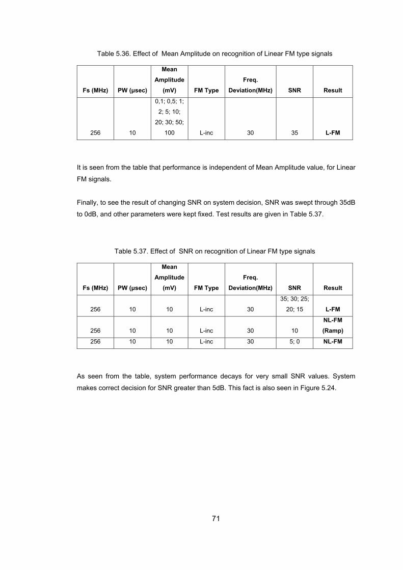
Table 5.36. Effect of Mean Amplitude on recognition of Linear FM type signals
Fs ( FM Type Deviation(MHz) SNR Result MHz) PW (µsec)
Mean Amplitude
(mV) Freq.
256 10
0,1; 0,5; 1;
2; 5; 10;
100 L-inc 30 35 L-FM 20; 30; 50;
It is seen from the table th nce is independent of Mean Amplitude value, for Linear
FM signals.
ina see the of ch N tem deci SNR was ept thr dB
ther parameters were kept fixed. Test results are given in Table 5.37.
Fs (MHz) PW (µsec)
Mean Amplitude
(mV) FM Type Freq.
Deviation(MHz) SNR Result
at performa
anging SF
to 0dB, and o
lly, to result R on sys sion, sw ough 35
Table 5.37. Effect of SNR on recognition of Linear FM type signals
256
35; 30; 25;
L-FM 10 10 L-inc 30 20; 15
256 10 L-inc 10
NL-FM (Ramp) 10 30
256 10 10 L-inc 30 5; 0 NL-FM
As s m the table, sys rfo ecays for very small SNR value
ake correct decision for SNR greater than 5dB. This fact is also seen in Figure 5.24.
een fro tem pe rmance d s. System
m s
71
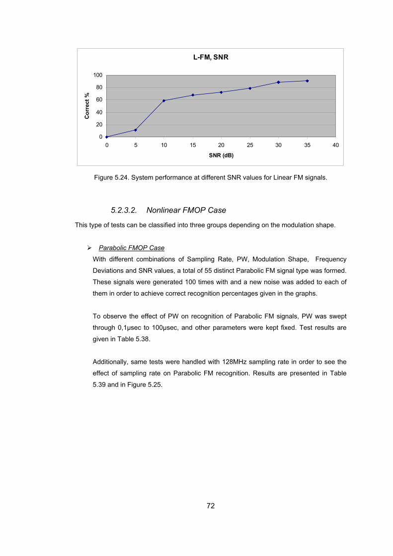
L-FM, SNR
0
20
40
60
80
100
0 5 10 15 20 25 30 35 40
SNR (dB)
Cor
rect
%
Figure 5.24. System performance at different SNR values for Linear FM signals.
This t on shape.
5.2.3.2. Nonlinear FMOP Case
ype of tests can be classified into three groups depending on the modulati
Parabolic FMOP Case
o observe the effect of PW on recognition of Parabolic FM signals, PW was swept
r to see the
ffect of sampling rate on Parabolic FM recognition. Results are presented in Table
.39 and in Figure 5.25.
With different combinations of Sampling Rate, PW, Modulation Shape, Frequency
Deviations and SNR values, a total of 55 distinct Parabolic FM signal type was formed.
These signals were generated 100 times with and a new noise was added to each of
them in order to achieve correct recognition percentages given in the graphs.
T
through 0,1µsec to 100µsec, and other parameters were kept fixed. Test results are
given in Table 5.38.
Additionally, same tests were handled with 128MHz sampling rate in orde
e
5
72
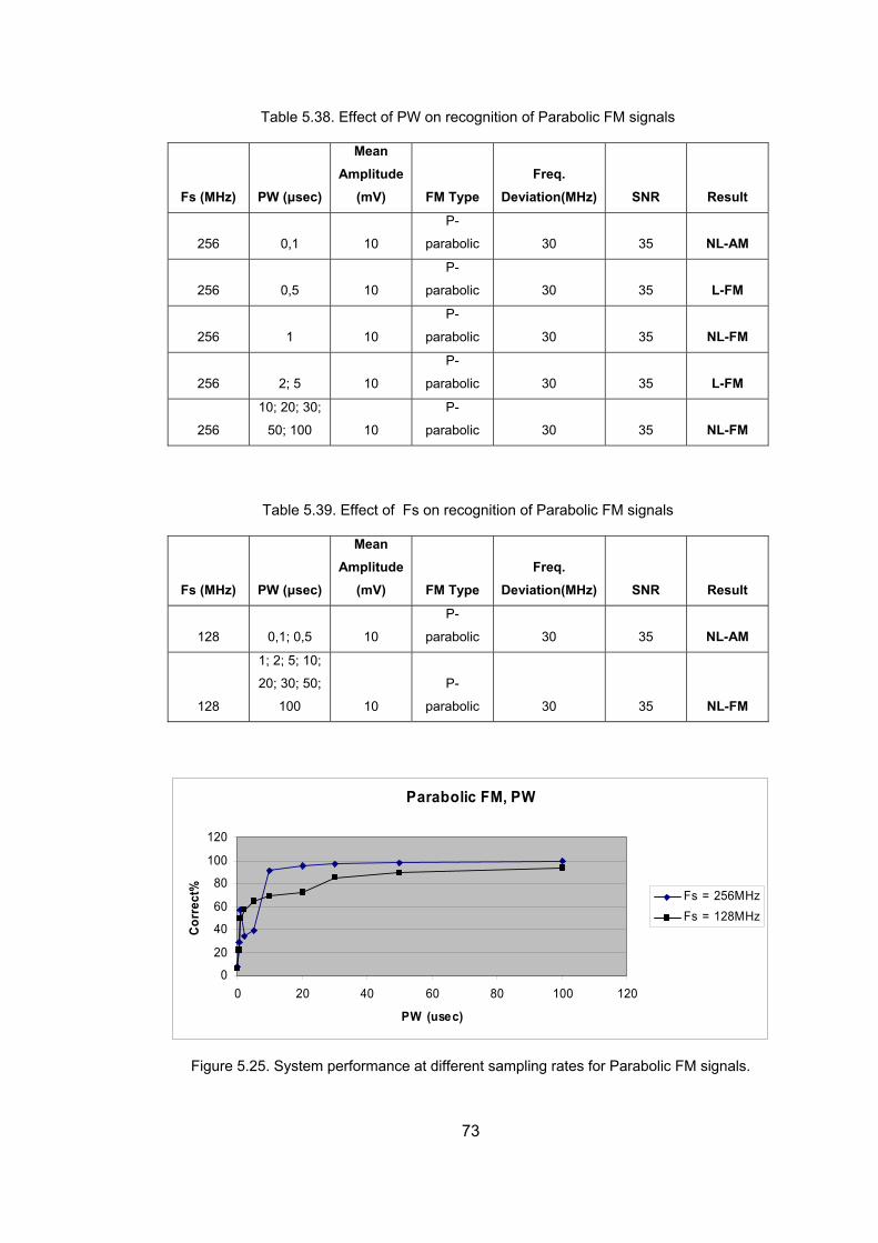
T
PW
able 5.38. Effect of PW on recognition of Parabolic FM signals
Fs (MHz) (µsec)
Mean Amplitude
(mV) FM Type Freq.
Deviation(MHz) SNR Result
256 0,1 10
P-
parabolic 30 35 NL-AM
256 0,5 10
P-
parabolic 30 35 L-FM
256 1 10 parabolic 30 35 NL-FM P-
256
P-
L-FM 2; 5 10 parabolic 30 35
256
10; 20; 30;
50; 10 10
P-
parab 30 35 NL-FM 0 olic
ble 5.39. Effect of Fs on recognition of Parabolic FM signals
Fs (MHz
MeAmp
(mV) FM Type Fr
Deviation(MHz) SNR Result
Ta
) PW (µsec)
an litude eq.
128 ,1; 0,5 1
P-
rabol 3 N0 0 pa ic 0 35 L-AM
1
1; 2; 5; 10;
20; 30; 50; P-
28 100 10 parabolic 30 35 NL-FM
Parabolic FM, PW
00 20 40 60 80 100 120
PW (usec)
20
40
60
100
0
Cor
rect
%
12
80Fs = 256MHzFs = 128MHz
Figure 5.25. System performance at different sampling rates for Parabolic FM signals.
73

7 and 5.38, we ake correct decision for
reater than 0 lso en beh n a s y
for both sampling rates.
Another data set was produced to see ect of Frequency Deviation value on the
cog n perfo nce tem easur s effect, F uency n
as swept throu 70MHz to 1MHz for constant va of all oth aramet est
results are given in Table 5.40.
Table 5.40. E
Fs (
Referrin
PW
g to
values g
Tables 5.3 see that sy
it is se
stem can m
that system,5µsec. A aves i imilar wa
the eff
. To mre nitio rma of the sys e thi req Deviatio
w gh lues er p ers. T
ffect of Frequency Deviation on recognition of Parabolic FM signals
MHz) PW (µsec)
Mean Amplitude
(mV) FM Type Freq.
Deviation(MHz) SNR Result
256 10
P-
parabolic
70; 60; 50; 40;
30; 20 35 NL-FM 10
256 10 10
P-
parabolic 15 35 L-FM
256 10 10
P-
parabolic 10 35 NL-FM
256 10 10
P-
parabolic 5; 1 35 No Mod.
As given in the table above, for a fixed PW value system performance gets better as
the Frequency Deviation increases, since the change in the signal frequency becomes
more obvious. For Frequency Deviation values less than 5MHz, modulation on
frequency becomes unobservable such that signal is confused with modulationless
pure signals. These facts can also be observed from the figure below.
74
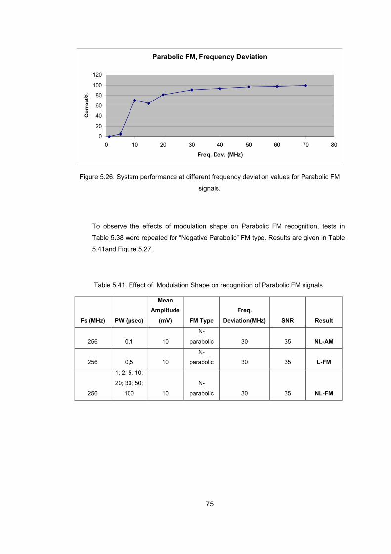
Parabolic FM, Frequency Deviation
0
20
40
60
8
100ec
t% 0
120
0 10 20 30 40 50 60 70 80
Freq. Dev. (MHz)
Cor
r
Figure 5.26. System performan quency deviation value
signals.
o ob ve the effects of lation pe on P olic FM recognition in
able 8 were eated abolic” e. Results are give le
5.41a igure 5.27.
Table 5.41. Effect of Modulation Shape n recognition of Parabolic FM signals
Fs (MHz) PW (µsec)
Mean Amplitude
(mV) FM Type Freq.
Deviation(MHz) SNR Result
ce at different fre s for Parabolic FM
T ser modu sha arab , tests
T 5.3 rep for “Negative Par FM typ n in Tab
nd F
o
256 0,1 10
N-
parabolic 30 35 NL-AM
256 0,5 10
N-
parabolic 30 35 L-FM
256
1; 2; 5; 10;
20; 30; 50;
100 10
N-
parabolic 30 35 NL-FM
75
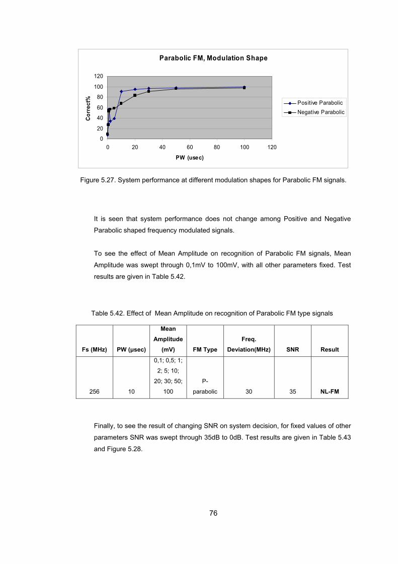
Parabolic FM, Modulation Shape
0
0
0 20 40 60 80 100 120
Cor
rect
%
12
40
60
80
100
Positive ParabolicNegative Parabolic
20
PW (usec)
F 5.2 st ance at diffe or Parabolic FM signals.
It is seen that system performance does not change among Positive and Negative
sha signals.
T ct of Mean Amplitude on recognition of Parabolic FM type signals
Fs (MHz) PW (µsec)
Mean
(mV) FM Type Deviation(MHz) SNR Result
igure
7. Sy em perform rent modulation shapes f
Parabolic ped frequency modulated
To see the effect of Mean Amplitude on recognition of Parabolic FM signals, Mean
Amplitude was swept through 0,1mV to 100mV, with all other parameters fixed. Test
re given in Table 5.42. results a
able 5.42. Effe
Amplitude Freq.
256 10
,1; 0,5; 1;
; 10;
0; 30
100
P-
parabolic 30 35 NL-FM
0
2; 5
2 ; 50;
inally, to see the result of changing SNR on system decision, for fixed values of other
F
parameters SNR was swept through 35dB to 0dB. Test results are given in Table 5.43
and Figure 5.28.
76
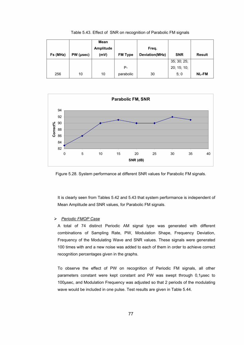
Table 5.43. Effect of SNR on recognition of Parabolic FM signals
Fs (MHz) PW (µsec)
Mean Amplitude
(mV) FM Type Freq.
Deviation(MHz) SNR Result
256 10 10
P-
parabolic 30
35; 30; 25;
20; 15; 10;
5; 0 NL-FM
Parabolic FM, SNR
94
82
84
86
0 5 10 15 20 25 30
8
90
8
2
35 40
SNR (dB)
Cor
rect
%
9
s seen from Tab at s orma indep of
ean plitude SNR r Pa olic FM s ls.
Periodic FMOP Case
Figure 5.28. System performance at different SNR values for Parabolic FM signals.
It i clearly les 5.42 and 5.43 th ystem perf nce is endent
M Am and values, fo rab igna
total of 74 distinct Periodic AM signal type was generated with different
combinations of Sampling Rate, PW, Modulation Shape, Frequency Deviation,
d
100 times with and a new noise was each of them in order to achieve correct
recognition percentages given in the graphs.
o observe the effect of PW on recognition of Periodic FM signals, all other
A
Frequency of the Modulating Wave and SNR values. These signals were generate
added to
T
parameters constant were kept constant and PW was swept through 0,1µsec to
100µsec, and Modulation Frequency was adjusted so that 2 periods of the modulating
wave would be included in one pulse. Test results are given in Table 5.44.
77
Table 5.44. Effect of PW on recognition of Periodic FM signals
z)
PW (µsec)
Mean Amplitude
(mV) FM Type
Freq. Deviation
(MHz) Modulation Freq(MHz) SNR Result
Fs(MH
256 20 35 NL-AM 0,1 10 Sinusoidal 30
256 0,5 10 Sinusoidal 30 4 35 NL-FM
256 1 10 Sinusoidal 30 2 35 L-FM
256
30;
50;
100 10 Sinusoidal 30 1 35 NL-FM
2; 5;
10;
20;
ame na o led bserve the effect of
m te o gniti erio Re en in 5.45.
ble 5.45. Effect of Fs on recognition of Periodic FM signals
(MHz) (µsec)
Mean Am
(mV) FM Type
Freq. Dn (MHz)
Mod tion Freq(MHz) SNR Result
S
sa
sig
pling ra
ls were als
n reco
samp
on of P
with 128M
dic FM.
Hz, in order to o
sults are giv Table
Ta
PW Fs plitude eviatio ula
128 0,1 10 Sinusoidal 30 20 35 L-AM
128 NL-FM
0,5; 1;
2 10 Sinusoidal 30 4 35
128 5 10 Sinusoidal 30 0,4 35 L-FM
128
10; 20;
30; 50;
100 NL-FM 10 Sinusoidal 30 0,2 35
fe the d 5.4 see m ca gnize ic
MOP pe sign even fo W valu reater tha sec. Also see th m
erfo ce is a oximat sam r both of the sampling s, whic
bse rom the figure be .
Re rring to Tables 5.44 an 5 it is n that syste n reco “Period
F ” ty als r P es g n 2µ we at, syste
p rman ppr ely the e fo rate h can be
o rved f low
78
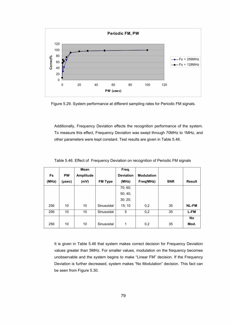
Periodic FM, PW
0
20
12
40
60
80
100
0
0 20 40 60 80 100 120
PW (usec)
Cor
rect
%
Fs = 256MHzFs = 128MHz
Figure 5.29. System performance at different sampling rates for Periodic FM signals.
Additionally, Frequency Deviation effects the recognition performance of the system.
To measure this effect, Frequency Deviation was swept through 70MHz to 1MHz, and
other parameters were kept constant. Test results are given in Table 5.46.
Fs (MHz)
PW (µsec)
Mean Amplitude
(mV) FM Type
Freq. Deviation
(MHz) Modulation Freq(MHz) SNR Result
Table 5.46. Effect of Frequency Deviation on recognition of Periodic FM signals
256 10 10 Sinusoidal 15; 10 0,2 35 NL-FM
70; 60;
50; 40;
30; 20;
256 10 10 Sinusoidal 5 0,2 35 L-FM
256 10 10 Sinusoidal 1 0,2 35
o Mod. N
s n Ta 46 t tem co n for cy Deviation
values greater than 5MHz. For smalle dulation on the frequency becomes
nobs ble an e system begins ke “Lin M” decisi If the F cy
evia is furth ecreased, system akes “No ulation” de on. Thi an
e seen from Figure 5.30.
It i given i ble 5. hat sys makes rrect decisio Frequen
r values, mo
to mau erva d th ear F on. requen
D tion er d m Mod cisi s fact c
b
79
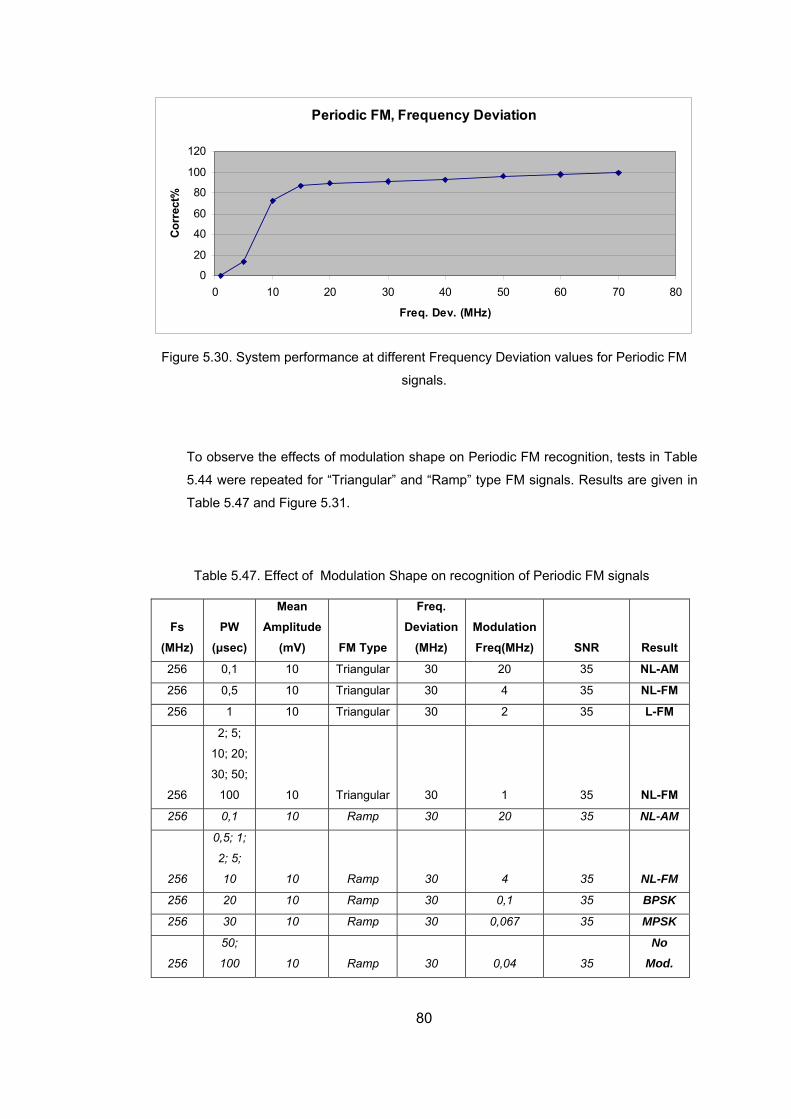
Periodic FM, Frequency Deviation
60
80
100
120
0
20
40
0 10 20 30 40 50 60 70 80
Cor
rect
%
Freq. Dev. (MHz)
Figure 5.30. System performance at different Frequency Deviation values for Periodic FM
o observe the effects of modulation shape on Periodic FM recognition, tests in Table
.44 were repeated for “Triangular” and “Ramp” type FM signals. Results are given in
Table
a . Ef Mo n Sh rec eriod signa
(MHz) (µsec)
Mean Am
(mV) FM Type
q. D tion
(MHz) Mo Freq(MHz) SNR Result
signals.
T
5
5.47 and Figure 5.31.
T ble 5.47 fect of dulatio ape on ognition of P ic FM ls
Fs PW plitudeFre
evia dulation
256 0,1 10 Triangular 30 20 35 NL-AM
256 0,5 10 Triangular 30 4 35 NL-FM
256 1 10 Triangular 30 2 35 L-FM
256
2; 5;
10; 20;
30; 50;
100 10 Triangular 30 1 35 NL-FM
256 0,1 10 Ramp 30 20 35 NL-AM
256
0,5; 1;
2; 5;
10 10 Ramp 30 4 35 NL-FM
256 20 10 Ramp 30 0,1 35 BPSK
256 30 10 Ramp 30 0,067 35 MPSK
256
50;
100 10 Ramp 30 0,04 35
No Mod.
80
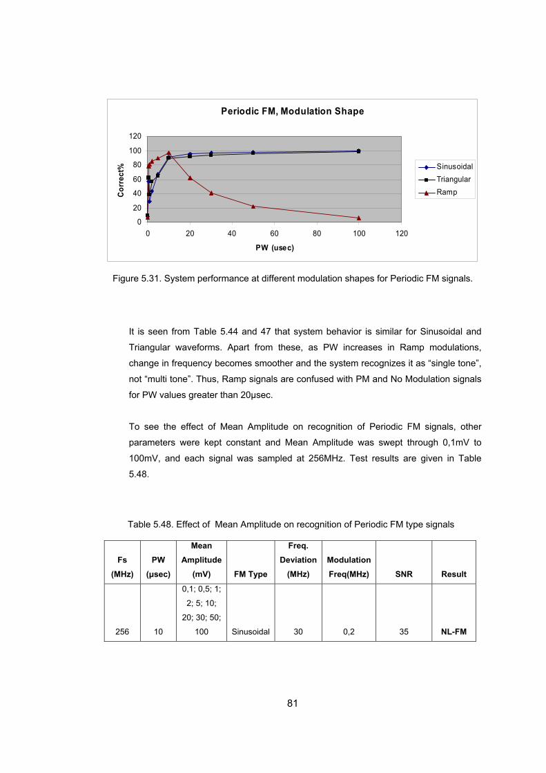
Periodic FM, Modulation Shape
20
00 20 40 60 80 100 120
PW
40
60
80
100
120
(usec)
Cor
rect
% SinusoidalTriangularRamp
Figure 5.31. System performance at different modulation shapes for Periodic FM signals.
fro 4 47 that milar for Sinusoidal and
a wav om as s in p mo s,
change in fre mes smoother and the system recognizes it as “single tone”,
not “multi tone Ramp signals are confused with PM and No Modulation signals
for PW value an 20µsec.
o see the effect of Mean Amplitude on recognition of Periodic FM signals, other
arameters were kept constant and Mean Amplitude was swept through 0,1mV to
able 5.48. Effect of Mean Amplitude on recognition of Periodic FM type signals
Fs (MHz)
PW (µsec)
Am e F
Modulation SNR Result
It is seen
Tri
m Table 5.4
eforms. A
and
part fr
system
these,
behavior is si
PW increasengular Ram dulation
quency beco
”. Thus,
s greater th
T
p
100mV, and each signal was sampled at 256MHz. Test results are given in Table
5.48.
T
Mean Freq. plitud(mV) M Type
Deviation (MHz) Freq(MHz)
256 10
0,1; 0,5; 1;
2; 5; 10;
20; 30; 50;
Si al 100 nusoid 30 0,2 35 NL-FM
81
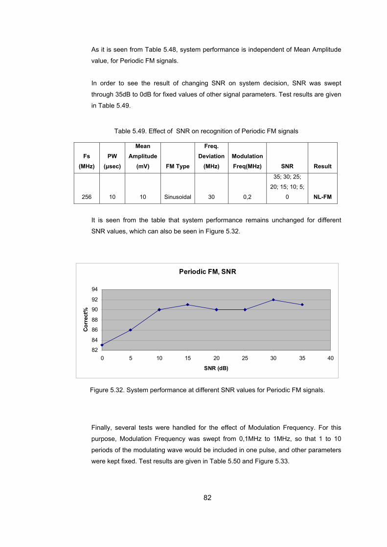
As it is seen from Table 5.48, system performance is independent of Mean Amplitude
value, for Periodic FM signals.
In order to see the result of changing SNR on system decision, SNR was swept
through 35dB to 0dB for fixed values of other signal parameters. Test results are given
in Table 5.49.
Table 5.49. Effect of SNR on recognition of Periodic FM signals
Fs (MHz) (µsec)
Mean
FM Type
Freq.
) SNR Result PW Amplitude Deviation Modulation
(mV) (MHz Freq(MHz)
256 10 10 Si al
35; 30; 25;
20; 15; 10; 5;
nusoid 30 0,2 0 NL-FM
It is seen from the table that system performance remains unchanged for different
SNR values, which can also be seen in Figure 5.32.
Periodic FM, SNR
82
84
86
88
90
92
0 5
94
10 15 20 25 30 35 40
SNR (dB)
Cor
rect
%
Figure 5.32. System performance at different SNR values for Periodic FM signals.
Finally, several tests were handled for the effect of Modulation Frequency. For this
purpose, M , so that 1 to 10
periods of the modulat e would be included in one pulse, and other parameters
were kept fi Tes g able 5. Figure 5.33.
odulation Frequency was swept from 0,1MHz to 1MHz
ing wav
t results arexed. iven in T 50 and
82
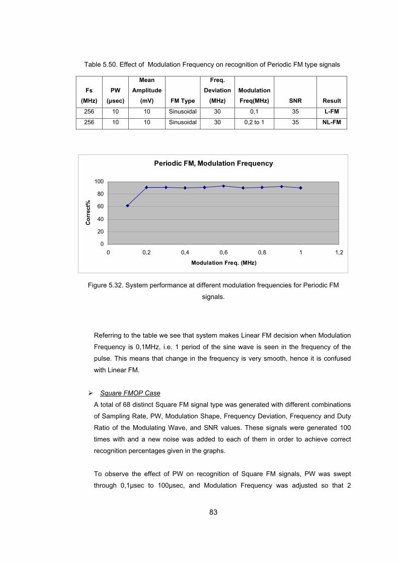
Table 5.50. Effect of Modulation Freque y on recogn of Period M typ ls
Fs (MHz
PW sec)
an itude V) Type
Freq. Deviation Modulation
Freq(MHz) R lt
nc ition ic F e signa
) (µ
MeAmpl
(m FM (MHz) SN Resu
256 10 10 Sinusoidal 30 0,1 35 L-FM
256 10 10 Sinusoidal 30 0,2 to 1 35 NL-FM
Periodic FM, Modulation Frequency
0
20
40
60
80
100
0 0,2 0,6 0,8 1 1,2
M Fr
Cor
rect
%
0,4
odulation eq. (MHz)
Figure 5.32. System performance at different modulat encies for Periodi
signals.
Referring to the table we see that system makes Linear FM decision when Modulation
Freq cy i eriod of the sine wave is seen in e freq
eans that change in the frequency is very smooth, hence it is confused
ith Linear FM.
ion frequ c FM
uen s 0,1MHz, i.e. 1 p th uency of the
pulse. This m
w
Square FMOP Case
A total of 68 distinct Square FM signal type was generated with different combinations
f Sampling Rate, PW, Modulation Shape, Frequency Deviation, Frequency and Duty
to each of them in order to achieve correct
cognition percentages given in the graphs.
, PW was swept
rough 0,1µsec to 100µsec, and Modulation Frequency was adjusted so that 2
o
Ratio of the Modulating Wave, and SNR values. These signals were generated 100
times with and a new noise was added
re
To observe the effect of PW on recognition of Square FM signals
th
83
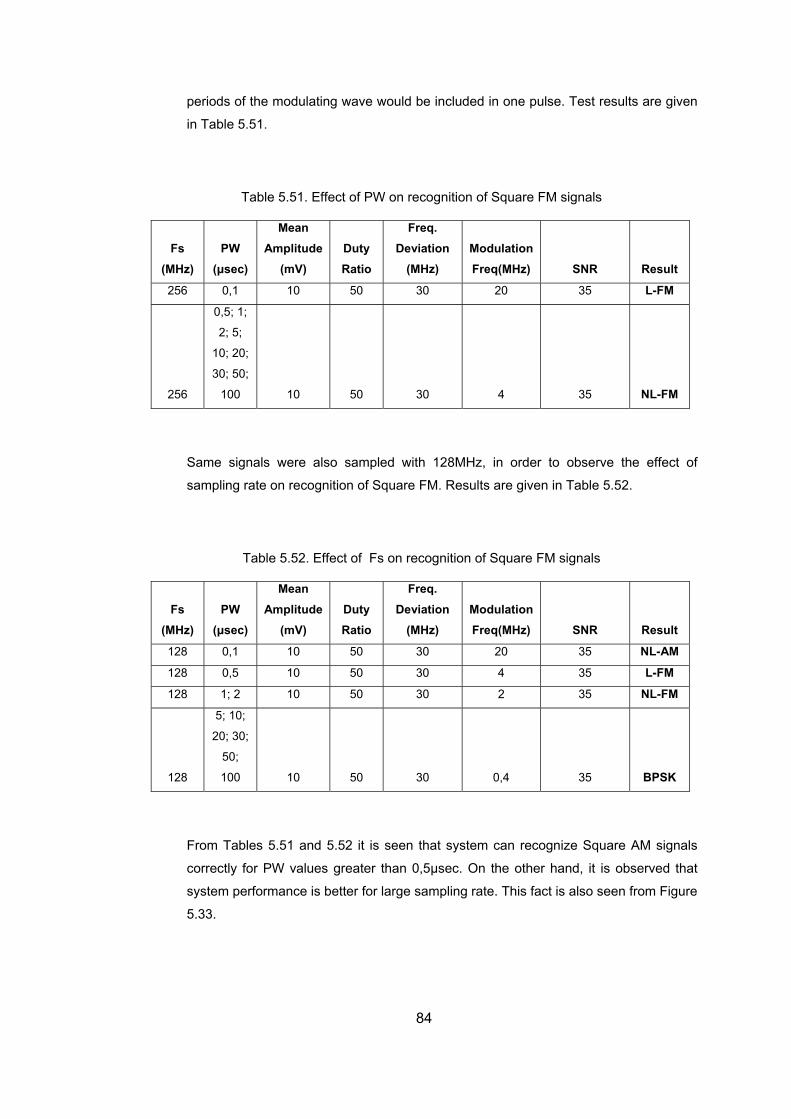
periods of the modulating wave would be included in one pulse. Test results are given
in T
1. E f PW o gn M s
F(MHz)
PW (µs
Mean plitude
)
Ratio
eq. D iation
(MHz) Mo tion Freq(MHz) SNR Result
able 5.51.
Table 5.5 ffect o n reco ition of Square F ignals
s ec) (mV
Am DutyFr
ev dula
256 0, 50 30 20 35 L-FM 1 10
256
0,5; 1;
2; 5
10; 20;
30; 5
100 10 50 30 4 35 NL-FM
;
0;
gnal also sampled with 128MHz, in r to o e effect of
sampling rate on recognition of Square FM. Results are given in Table 5.52.
Table 5.52 Fs nition re FM signals
Fs (MHz)
PW(µs
n tude )
Duty Ratio
. Deviation
(MHz) Modulation Freq(MHz) SNR Result
Same si s were orde bserve th
. Effect of on recog
Freq
of Squa
ec)
Ampli(mV
Mea
1 0,1 10 50 28 30 20 35 NL-AM
1 0,5 10 50 28 30 4 35 L-FM
128 1; 50 30 2 35 NL-FM 2 10
1
5;
20; 30;
50;
100 10 50 28
10;
30 0,4 35 BPSK
m Tabl 51 and it is seen that system can recognize uare A als
ectly fo values ater tha ,5µsec. On other han is obs at
system pe er for large sampling rate. This fact is also seen from Figure
Fro es 5. 5.52 Sq M sign
corr r PW gre n 0 the d, it erved th
rformance is bett
5.33.
84
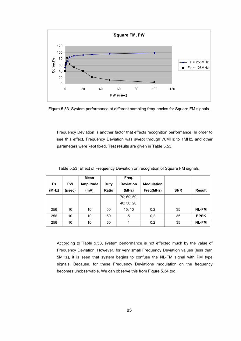
Square FM, PW
120
0
0
0 20 40 60 80 100 120
PW (usec)
Cor
rect
%10
20
40
60
80Fs = 256MHzFs = 128MHz
Figure 5.33. System performance at different sampling frequencies for Square FM signals.
Frequency Deviation is another factor that effects recognition performance. In order to
see this effect, Frequency Deviation was swept through 70MHz to 1MHz, and other
parameters were kept fixed. Test results are given in Table 5.53.
Table 5.53. Effect of Frequency Deviation on recognition of Square FM signals
Fs (MHz)
PW (µsec)
Amplitude (mV)
Duty Ratio
Deviation (MHz)
Modulation Freq(MHz) SNR Result
Mean Freq.
256
70; 60; 50;
10 10 50
40; 30; 20;
15; 10 0,2 35 NL-FM
256 5 0,2 35 BPSK 10 10 50
256 10 10 50 1 0,2 35 NL-FM
According to Table 5.53, system performance is not effected much by the value of
Frequency Deviation. H er, for very small Frequency Deviation values (less than
that begin with P type
signals. Because, for these Frequency D ulation on the frequency
becomes unobservable. We can observe this 34 too.
owev
system 5MHz), it is seen s to confuse the NL-FM signal M
eviations mod
from Figure 5.
85
Square FM, Frequency Deviation
120
100
0
20
40
0 10 20 30 40 50 60 70 80
60
80
Freq. Dev. (MHz)
Cor
rect
%
Figure 5.34. System perfo
order to observe the effects of Duty Ratio parameter on modulation recognition,
uty Ratio of the modulating square wave was swept from 5% to 99% for constant
value igure 5.35.
ble ffect of Duty Ra rec re nal
Fs (MHz)
PW (µsec)
MeanAmplitud
(mV)
Freq. Deviation
(MHz) Modulation Freq(MHz) SNR Result
rmance at different frequency deviations for Square FM signals.
In
D
s of all other parameters. Results are given both in Table 5.54 and in F
Ta 5.54. E tio on ognition of Squa FM sig s
e Duty
Ratio
256 10 10 90 M 5 to 30 0,2 35 NL-F
256 10 10 97; 99 30 0,2 35 BPSK
86
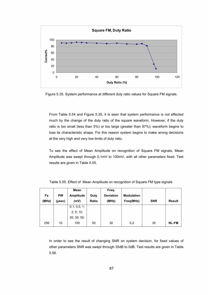
Square FM, Duty Ratio
0
20
40
00
0 60 80 100 120
Cor
rect
%
1
60
80
20 40
Duty Ratio (%)
Figure 5.35. System performance at different duty ratio values for Square FM signals.
From Table 5.54 and Figure 5.35, it is seen that system performance is not effected
, waveform begins to
lose its characteristic shape. For this reason system begins to make wrong decisions
at the very high and very low limits of duty ratio.
To see the effect of Mean Amplitude on recognition of Square FM signals, Mean
Amplitude was swept through 0,1mV to 100mV, with all other parameters fixed. Test
are g le 5.55
Table 5.55 an Amplitude on recognition of Square FM type signals
Fs PW Mean
Amplitude Duty Freq.
Deviation Modulation
much by the change of the duty ratio of the square waveform. However, if the duty
ratio is too small (less than 5%) or too large (greater than 97%)
results iven in Tab .
. Effect of Me
(MHz) (µsec) (mV) Ratio (MHz) Freq(MHz) SNR Result
256 10
0,1; 0,5; 1;
2; 5; 10;
20; 30; 50;
100 50 30 0,2 35 NL-FM
given in Table
5.56.
In order to see the result of changing SNR on system decision, for fixed values of
other parameters SNR was swept through 35dB to 0dB. Test results are
87
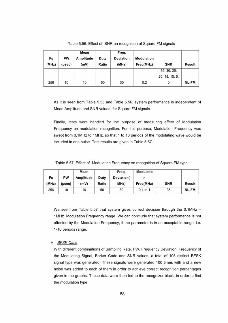
Table 5.56. Effect of SNR on recognition of Square FM signals
(MHW
(µsec)
Mean
) DuRatio
q. Devia
(MHz) tion
req(MHz) SNR Fs P
z) Amplitude
(mVty
Fre
tion Modula
F Result
256 10 50 30 0,2
; 30; 25;
20; 15; 10; 5;
0 10
35
NL-FM
Finally, tests were handled for the purpose of measuring effect of Modulation
Frequency on modulation recognition. For this purpose, Modulation Frequency was
swept from 0,1MHz to 1MHz, so that 1 to 10 periods of the modulating wave would be
included in one pulse. Test results are given in Table 5.57.
Table 5.57. Effect of Modulation Frequency on recognition of Square FM type
Fs (MHz)
PW (µsec)
Mean Amplitude
(mV) Duty Ratio
Freq. Deviation(
MHz)
Modulation
Freq(MHz) SNR Result
As it is seen from Table 5.55 and Table 5.56, system performance is independent of
Mean Amplitude and SNR values, for Square FM signals.
256 10 10 50 30 0,1 to 1 35 NL-FM
W Hz –
1MHz Modulation Frequency range. We can conclude that system performance is not
effected by the Modulation Frequency, if the parameter is in an acceptable range, i.e.
BFSK Case
e see from Table 5.57 that system gives correct decision through the 0,1M
1-10 periods range.
With different combinations of Sampling Rate, PW, Frequency Deviation, Frequency of
the Modulati ct BFSK
signal type was generated. These signals were generated 100 times with and a new
noise was added to each of them in order to achieve correct recognition percentages
given in the graphs. These then fed to the recognizer block, in order to find
ng Signal, Barker Code and SNR values, a total of 105 distin
data were
the modulation type.
88
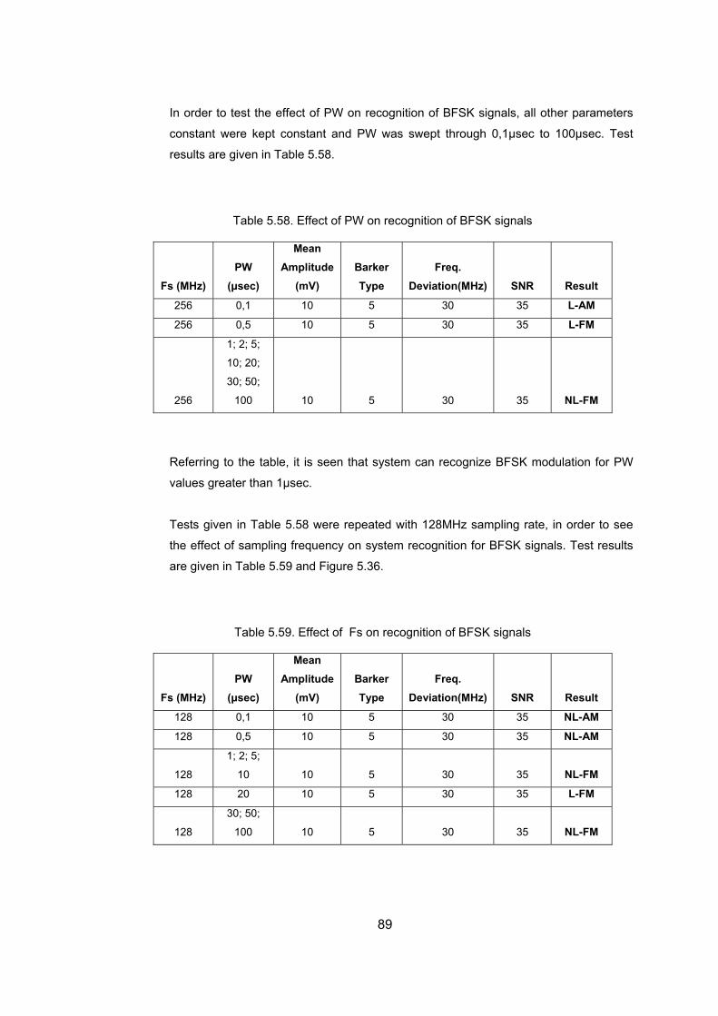
In order to test the effect of PW on recognition of BFSK sign all other eters
tant were kept constant and PW was swept through 0,1µsec to 10 est
results are e 5.58.
Table 5.58. Effect of PW on recognition of BFSK signals
Fs (MHz) P
(µse
mplitude
(mV) Barker Type
Freq. D ation(MHz) SNR Result
als, param
cons 0µsec. T
given in Tabl
W Mean
Ac)
evi
256 0,1 10 5 30 L 35 -AM
256 0,5 10 5 30 35 L-FM
256
10
30; 5
100 10 5 30 5 N
1; 2; 5;
; 20;
0;
3 L-FM
rring to it is see at system c recognize BFSK modula PW
s greate µsec.
s given in Table 5.58 were repeated with 128MHz sampli
ffect of frequency on system re nition for B signals. sults
iven in Table 5.59 and Figure 5.36.
Table 5.59. Effect of Fs on recognition of BFSK signals
PW Mean
Amplitude Barker Freq.
Refe the table, n th an tion for
value r than 1
Test ng rate, in order to see
the e sampling cog FSK Test re
are g
Fs (MHz) (µsec) (mV) Type Deviation(MHz) SNR Result
128 0,1 10 5 30 35 NL-AM
128 0,5 10 5 30 35 NL-AM
128 10 10 5 30 35 NL-FM 1; 2; 5;
128 20 10 5 30 35 L-FM
128 100 10 5 30 35 NL-FM 30; 50;
89
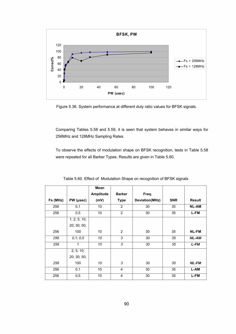
BFSK, PW
120
0
20
40
60
80
100
40 0
Cor
rect
%
Fs = 256MHzFs =
0 20 60 80 10 120
PW (usec)
128MHz
re 5.36. Sy perform different duty ratio values for BFSK sig
Table 5.60. E
Fs (MHz) PW (µsec)
Meanplitude(mV)
ker Type
.
Figu stem ance at nals.
Comparing Tables 5.58 and 5.59, it is seen that system behaves in similar ways for
256MHz and 128MHz Sampling Rates.
To observe the effects of modulation shape on BFSK recognition, tests in Table 5.58
were repeated for all Barker Types. Results are given in Table 5.60.
ffect of Modulation Shape on recognition of BFSK signals
BarAm Freq
Deviation(MHz) SNR Result
256 0,1 10 2 30 35 NL-AM
256 0,5 10 2 30 35 L-FM
256
1; 2; 5; 10;
20; 30; 50;
100 10 2 30 35 NL-FM
256 0,1; 0,5 10 3 30 35 NL-AM
256 1 10 3 30 35 L-FM
256
20; 30; 50;
100 10 3 30 35 NL-FM
2; 5; 10;
256 0,1 10 4 30 35 L-AM
256 0,5 10 4 30 35 L-FM
90
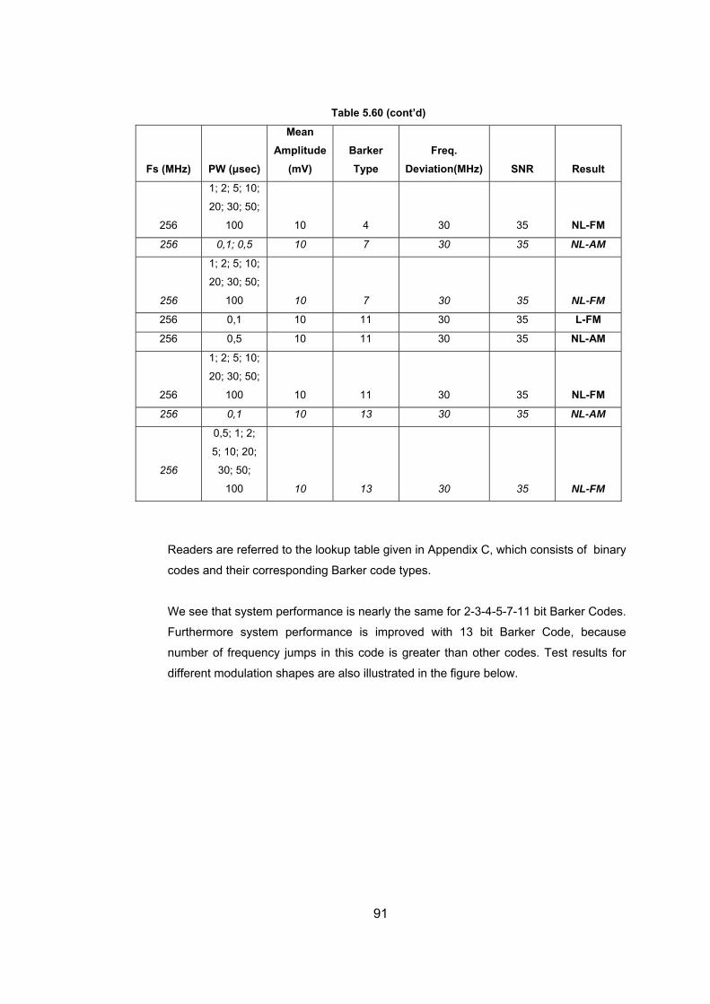
Table 5.60 (cont’d)
Fs (MHz) PW (µsec)
Mean Amplitude
(mV) Barker Type
Freq. Deviation(MHz) SNR Result
256
1; 2; 5; 10;
20; 30; 50;
100 10 4 30 35 NL-FM
256 0,1; 0,5 10 7 30 35 NL-AM
256
1; 2; 5; 10;
20; 30; 50;
100 10 7 30 35 NL-FM
256 FM 0,1 10 11 30 35 L-
256 0,5 10 11 30 35 NL-AM
256
1; 2; 5; 10;
20; 30; 50;
30 35 NL-FM 100 10 11
256 0,1 10 13 30 35 NL-AM
256
0,5; 1; 2;
5; 10; 20;
30; 50;
100 10 13 30 35 NL-FM
Readers are referred to the lookup table given in Appendix C, which consists of binary
We see that system performance is nearly the same for 2-3-4-5-7-11 bit Barker Codes.
Furthermore system performance is improved with 13 bit Barker Code, because
number of sults for
different modulation shapes are also illustrated in the figure below.
codes and their corresponding Barker code types.
frequency jumps in this code is greater than other codes. Test re
91
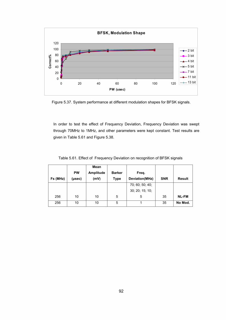
BFSK, Modulation Shape
0
20
40
120
0 120
(usec)
Co
60
80
100rr
ect%
2 bit3 bit
20 40 60 80 100
PW
4 bit5 bit7 bit11 bit13 bit
.37. forman differe n shap r BFSK s
rder to test the effect of Frequency Deviation, Frequen Deviation ept
h 70 and other paramete pt con tant. Test re
in Tabl gure 8.
Table 5.61. Effect of Frequency Deviation on recognition of BFSK signals
Fs (MHz) PW
(µsec) Amplitude
(mV) Barker Type
Freq. Deviation(MHz) SNR Result
Figure 5 System per ce at nt modulatio es fo ignals.
In o cy was sw
throug MHz to 1MHz,
e 5.61 and Fi
rs were ke s results a
given 5.3
Mean
256 10 10 5
70; 60; 50; 40;
5 35 NL-FM 30; 20; 15; 10;
256 10 10 5 1 35 No Mod.
92
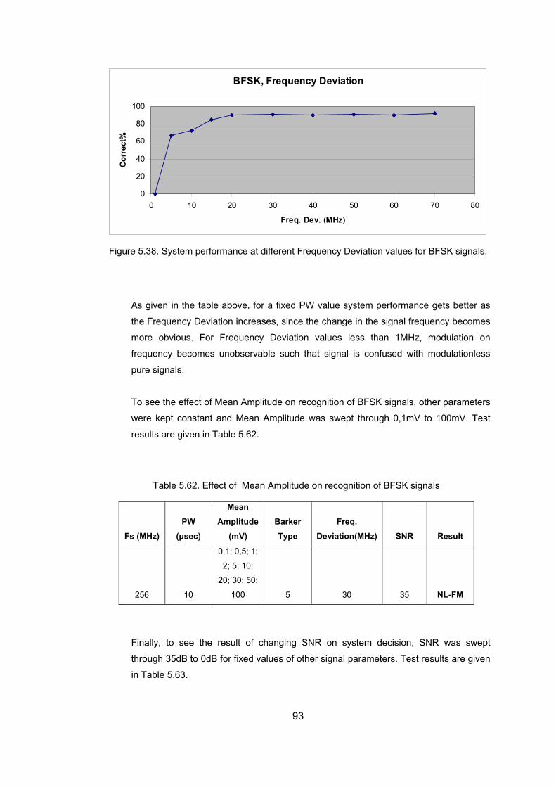
BFSK, Frequency D ation
40
60
0 10 20 30 40 50 60 70 80
Cor
rect
%
evi
0
20
80
100
Freq. Dev. (MHz)
Figure 5.38. System performance at different Frequency Deviation values for BFSK signals.
As given in the table above, for a fixed PW value system performance gets better as
the Frequency Deviation increases, since the change in the signal frequency becomes
more obvious. For Frequency Deviation values less than 1MHz, modulation on
frequency becomes unobservable such that signal is confused with modulationless
pure signals.
To see the effect of Mean Amplitude on recognition of BFSK signals, other parameters
were kept constant and Mean Amplitude was swept through 0,1mV to 100mV. Test
results are given in Table 5.62.
Table 5.62. Effect of Mean Amplitude on recognition of BFSK signals
Mean
Fs (MHz) PW
(µsec) Amplitude
(mV) Barker Type
Freq. Deviation(MHz) SNR Result
0,1; 0,5; 1;
2; 5; 10;
256 10 100 5 30 35 NL-FM 20; 30; 50;
Finally, to see the result of changing SNR on system decision, SNR was swept
through 35dB to 0dB for fixed values of other signal parameters. Test results are given
in Table 5.63.
93
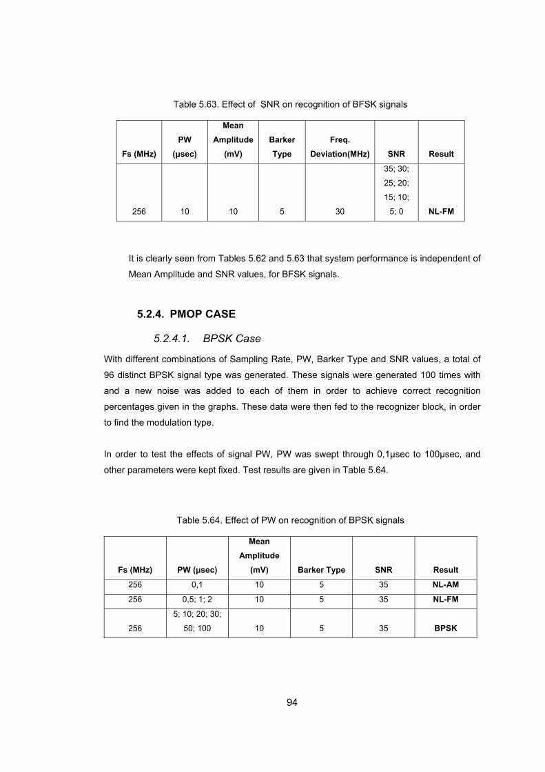
Table 5.63. Effect R on r f BFSK als
Fs (MHz) PW
(µsec)
MeAmplitu
(mV) rker
Type Freq.
Deviation(MHz) SNR Result
of SN ecognition o sign
an de Ba
256 10 10
25; 20;
5 30
35; 30;
15; 10;
5; 0 NL-FM
Mean Amplitude and SNR values, for BFSK signals.
5.2.4.
5.2.4.1. BPSK Ca
With different combinations of Sa e, PW, Barker Type and SNR values, a total of
96 di PSK signal ty generated. Th
and a noise w added to e of them in rder to rrect ition
perce s given in the graphs. Th t fed to the recognizer block, in order
find the modulation type.
In order to test the effects of signal PW, PW as swept through 0,1µsec to 100µsec, and
other parameters were kept fixed. Test results are given in Table 5.64.
Table 5.64. Effect of PW on recognition of BPSK signals
Fs (MHz) PW (µsec)
Mean Amplitude
(mV) Barker Type SNR Result
It is clearly seen from Tables 5.62 and 5.63 that system performance is independent of
PMOP CASE
se
mpling Rat
stinct B pe was ese signals were generated 100
achieve co
times with
new as ach o recogn
ntage ese data were hen
to
w
256 0,1 10 5 35 NL-AM
256 0,5; 1; 2 10 5 35 NL-FM
256
5; 10; 20; 30;
50; 100 10 5 35 BPSK
94
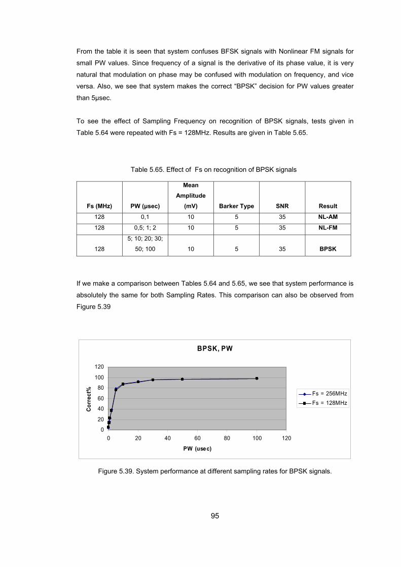
From the table it is seen that system confuses BFSK signals with Nonlinear FM signals for
small PW values. Since frequency of a signal is the derivative of its phase value, it is very
natural that modulation on phase may be confused with modulation on frequency, and vice
versa. Also, we see that system makes the correct “BPSK” decision for PW values greater
than 5µsec.
To see the effect of Sampling Frequency on recognition of BPSK signals, tests given in
Table 5.64 were rep d with Fs = 128MHz. Results are given in Table 5.65.
Table 5.65. Effect of Fs on recognition of BPSK signals
Fs (MHz) PW sec)
Mean Amplitude
(mV) Barker Type SNR Result
eate
(µ
128 0,1 10 5 35 NL-AM
128 0,5; 1; 2 10 5 35 NL-FM
128
5; 10; 20; 30;
10 5 35 BPSK 50; 100
If we make a compa n between Tables 5.64 and 5.65, we see that system performance is
absolutely the same oth Sampling Rates. This comparison can also be observed from
Figure 5.39
riso
for b
BPSK, PW
0
20
40
60
80
100
120
0 20 40 60 80 100 120
PW (usec)
Cor
rect
%
Fs = 256MHzFs = 128MHz
Figure 5.39. System performance at different sampling rates for BPSK signals.
95
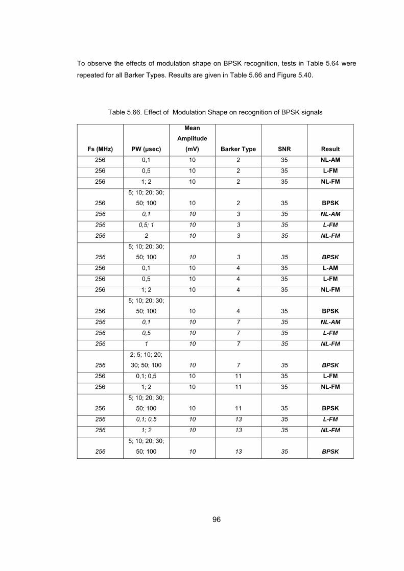
To observe the effects of modulation shape on BPSK recognition, tests in Table 5.64 were
repeated for all Barker Types. Results are given in Table 5.66 and Figure 5.40.
Table 5.66. Effect of Modulation Shape on recognition of BPSK signals
Fs (MHz) P
Mean Amplitude
Result W (µsec) (mV) Barker Type SNR
256 0,1 10 35 NL-AM 2
256 0 10 2 35 L-FM ,5
256 1; 2 10 NL2 35 -FM
256
5; 10; 20; 30;
50; 100 2 35 BPS10 K
256 0 35 NL-A,1 10 3 M
0,5 35 L-FM 256 ; 1 10 3
2 NL256 10 3 35 -FM
256
5; 10; 20; 30;
50; 100 0 3 35 B1 PSK
256 0,1 10 4 35 L-AM
256 0,5 10 4 35 L-FM
256 1; 2 10 4 35 NL-FM
256
5; 10; 20; 30;
50; 100 10 4 35 BPSK
256 0,1 10 7 35 NL-AM
256 0,5 10 7 35 L-FM
256 1 10 7 35 NL-FM
25 7 35 BPSK 6
2; 5; 10; 20;
30; 50; 100 10
2 6 0,1; 0,5 10 11 35 L-FM 5
25 11 35 NL-FM 6 1; 2 10
256
5; 10; 20; 30;
50; 100 10 11 35 BPSK
256 0,1; 0,5 10 13 35 L-FM
256 1; 2 10 13 35 NL-FM
256
5; 10; 20; 30;
50; 100 10 13 35 BPSK
96
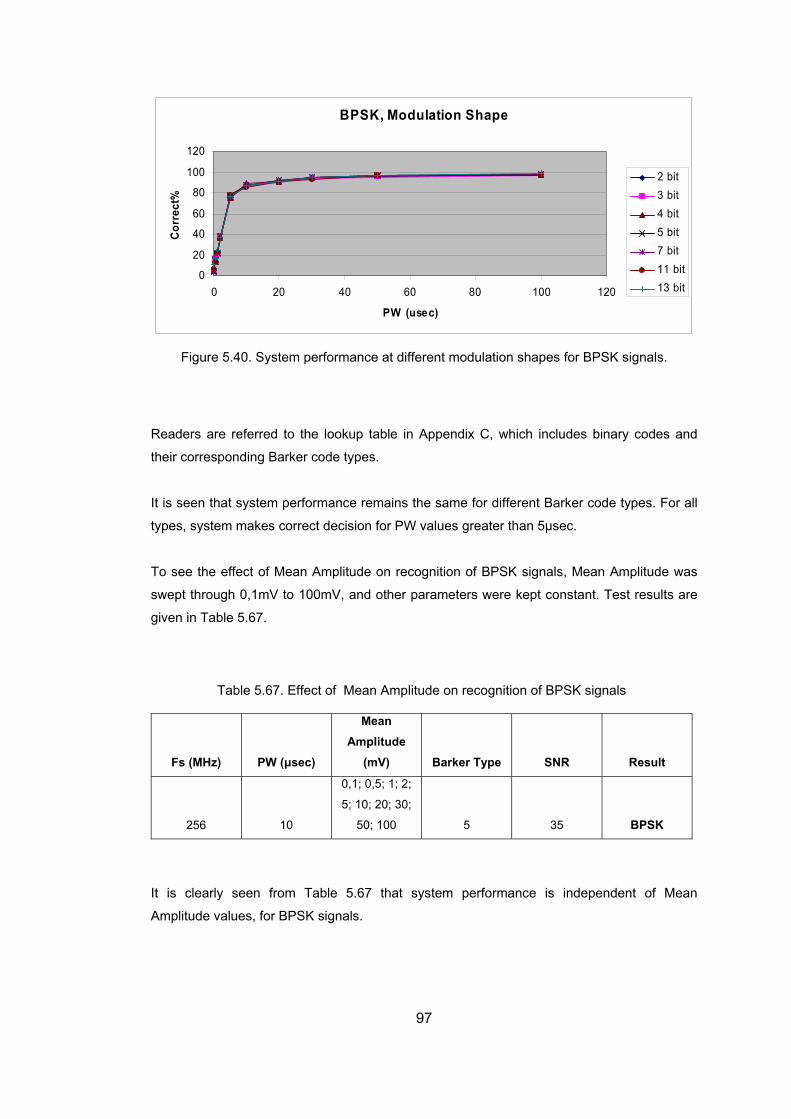
BPSK, Modulation Shape
0
0
0
0
2
4
6
8
12
Cor
rect
%
0
0
100
0 20 40 60 80 100 120
PW (usec)
2 bit3 bit4 bit5 bit7 bit11 bit13 bit
eaders are referred to the lookup table in Appendix C, which includes binary codes and
their corresponding Ba
It is seen that sy nce remai e for different Barker code types. For all
types, system makes t decision for PW values greater than
To see the effect of Mean Amplitude on n of BPSK si ean Amplitude was
swept through 0,1mV to 100mV, and othe eters were kep re
given in Table 5.67.
Figure 5.40. System performance at different modulation shapes for BPSK signals.
R
rker code types.
stem performa ns the sam
correc 5µsec.
recognitio gnals, M
r param t constant. Test results a
Table 5.67. Effect of Mean Amplitude on recognition of BPSK signals
Fs (MHz) PW (µsec)
Mean Amplitude
(mV) Barker Type SNR Result
256 10
0,1; 0,5; 1; 2;
5; 10; 20; 30;
50; 100 5 35 BPSK
It is clearly seen from Table 5.67 that system performance is independent of Mean
Amplitude values, for BPSK signals.
97
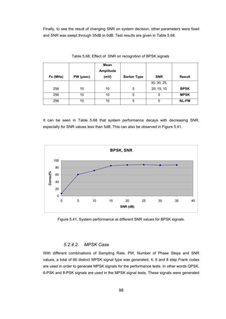
Finally, to see the result of changing SNR on system decision, other parameters were fixed
and SNR was
68. NR og f B
Fs (MHz) sec)
an tude V) Barker T NR Result
swept through 35dB to 0dB. Test results are given in Table 5.68.
Table 5. Effect of S on rec nition o PSK signals
PW (µ
MeAmpli
(m ype S
256 10 10
35; 30; 25;
10 BPSK 5 20; 15;
256 10 10 5 MPSK 5
256 10 10 5 NL-FM 0
It can be seen in Table 5.68 that system performance decays with decreasing SNR,
especially for SNR values less than 5dB. This can also be observed in Figure 5.41.
BPSK, SNR
100
00
20
40
60
80
B)
Cor
rect
%
5 10 15 20 25 30 35 40
SNR (d
5.41. Sys m perfo a t S K signals.
5.2.4.2. MPSK Case
With different combinations of Sampling Rate, PW, Number of Phase Steps and SNR
values, a total of 66 distinct MPSK signal type was generated. 4, 6 and 8 step Frank codes
are used in order to generate MPSK signals for the performance tests. In other words QPSK,
6-PSK and 8-PSK signals are used in the MPSK signal tests. These signals were generated
Figure te rmance t differen NR values for BPS
98
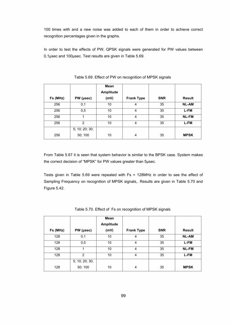
100 times with and a new noise was added to each of them in order to achieve correct
recognition percentages given in the graphs.
In order to test the effects of PW, QPSK signals were generated for PW values between
0,1µsec and 100µsec. Test results are given in Table 5.69.
Table 5.69. Effect of PW on recognition of MPSK signals
Fs (MHz) PW (µsec)
Mean Amplitude
(mV) Frank Type SNR Result
256 0,1 10 4 35 NL-AM
256 0,5 10 4 35 L-FM
256 1 10 4 35 NL-FM
256 2 10 4 35 L-FM
256
5; 10; 20; 30;
50; 100 10 4 35 MPSK
From Table 5.67 it is seen that system behavior is similar to the BPSK case. System makes
the correct decision of “MPSK” for PW values greater than 5µsec.
Tests given in Table 5.69 were repeated with Fs = 128MHz in order to see the effect of
Sampling Frequency on recognition of MPSK signals,. Results are given in Table 5.70 and
Figure 5.42.
Table 5.70. Effect of Fs on recognition of MPSK signals
Fs (MHz) PW (µsec)
Mean Amplitude
(mV) Frank Type SNR Result
128 0,1 10 4 35 NL-AM
128 0,5 10 4 35 L-FM
128 1 10 4 35 NL-FM
128 2 10 4 35 L-FM
128
5; 10; 20; 30;
50; 100 10 4 35 MPSK
99
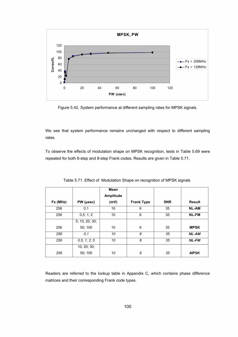
MPSK, PW
0
20
40
60
80
100
120
0 20 40 60 80 100 120
PW (usec)
Cor
rect
%
Fs = 256MHzFs = 128MHz
Figure 5.42. System performance at different sampling rates for MPSK signals.
We see that system performance remains unchanged with respect to different sampling
rates.
To observe the effects of modulation shape on MPSK recognition, tests in Table 5.69 were
repeated for both 6-step and 8-step Frank codes. Results are given in Table 5.71.
Table 5.71. Effect of Modulation Shape on recognition of MPSK signals
Fs (MHz) PW (µsec)
Mean Amplitude
(mV) Frank Type SNR Result
256 0,1 10 6 35 NL-AM
256 0,5; 1; 2 10 6 35 NL-FM
256
5; 10; 20; 30;
50; 100 10 6 35 MPSK
256 0,1 10 8 35 NL-AM
256 0,5; 1; 2; 5 10 8 35 NL-FM
256
10; 20; 30;
50; 100 10 8 35 MPSK
Readers are referred to the lookup table in Appendix C, which contains phase difference
matrices and their corresponding Frank code types.
100
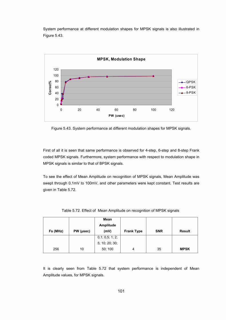
System performance at different modulation shapes for MPSK signals is also illustrated in
Figure 5.43.
MPSK, Modulation Shape
0
20
40
60
80
100
120
0 20 40 60 80 100 120
PW (usec)
Cor
rect
% QPSK6-PSK8-PSK
Figure 5.43. System performance at different modulation shapes for MPSK signals.
First of all it is seen that same performance is observed for 4-step, 6-step and 8-step Frank
coded MPSK signals. Furthermore, system performance with respect to modulation shape in
MPSK signals is similar to that of BPSK signals.
To see the effect of Mean Amplitude on recognition of MPSK signals, Mean Amplitude was
swept through 0,1mV to 100mV, and other parameters were kept constant. Test results are
given in Table 5.72.
Table 5.72. Effect of Mean Amplitude on recognition of MPSK signals
Fs (MHz) PW (µsec)
Mean Amplitude
(mV) Frank Type SNR Result
256 10
0,1; 0,5; 1; 2;
5; 10; 20; 30;
50; 100 4 35 MPSK
It is clearly seen from Table 5.72 that system performance is independent of Mean
Amplitude values, for MPSK signals.
101
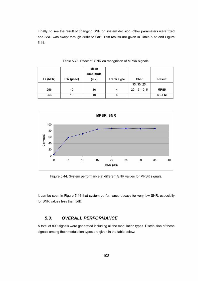
Finally, to see the result of changing SNR on system decision, other parameters were fixed
and SNR was swept through 35dB to 0dB. Test results are given in Table 5.73 and Figure
5.44.
Table 5.73. Effect of SNR on recognition of MPSK signals
Fs (MHz) PW (µsec)
Mean Amplitude
(mV) Frank Type SNR Result
256 10 10 4
35; 30; 25;
20; 15; 10; 5 MPSK
256 10 10 4 0 NL-FM
MPSK, SNR
0
20
40
60
80
100
0 5 10 15 20 25 30 35 40
SNR (dB)
Cor
rect
%
Figure 5.44. System performance at different SNR values for MPSK signals.
It can be seen in Figure 5.44 that system performance decays for very low SNR, especially
for SNR values less than 5dB.
5.3. OVERALL PERFORMANCE
A total of 800 signals were generated including all the modulation types. Distribution of these
signals among their modulation types are given in the table below:
102
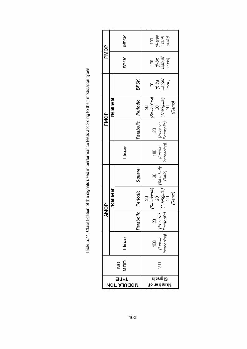
Tabl
e 5.
74. C
lass
ifica
tion
of th
e si
gnal
s us
ed in
per
form
ance
test
s ac
cord
ing
to th
eir m
odul
atio
n ty
pes
103
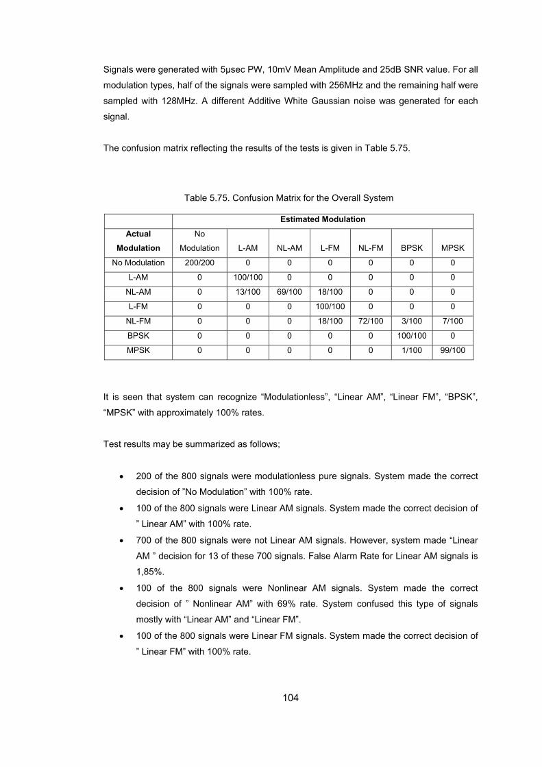
Signals were generated with 5µsec PW, 10mV Mean Amplitude and 25dB SNR value. For all
modulation types, half of the signals were sampled with 256MHz and the remaining half were
sampled with 128MHz. A different Additive White Gaussian noise was generated for each
signal.
The confusion matrix reflecting the results of the tests is given in Table 5.75.
Table 5.75. Confusion Matrix for the Overall System
Estimated Modulation
Actual Modulation
No
Modulation L-AM NL-AM L-FM NL-FM BPSK MPSK
No Modulation 200/200 0 0 0 0 0 0
L-AM 0 100/100 0 0 0 0 0
NL-AM 0 13/100 69/100 18/100 0 0 0
L-FM 0 0 0 100/100 0 0 0
NL-FM 0 0 0 18/100 72/100 3/100 7/100
BPSK 0 0 0 0 0 100/100 0
MPSK 0 0 0 0 0 1/100 99/100
It is seen that system can recognize “Modulationless”, “Linear AM”, “Linear FM”, “BPSK”,
“MPSK” with approximately 100% rates.
Test results may be summarized as follows;
• 200 of the 800 signals were modulationless pure signals. System made the correct
decision of ”No Modulation” with 100% rate.
• 100 of the 800 signals were Linear AM signals. System made the correct decision of
” Linear AM” with 100% rate.
• 700 of the 800 signals were not Linear AM signals. However, system made “Linear
AM ” decision for 13 of these 700 signals. False Alarm Rate for Linear AM signals is
1,85%.
• 100 of the 800 signals were Nonlinear AM signals. System made the correct
decision of ” Nonlinear AM” with 69% rate. System confused this type of signals
mostly with “Linear AM” and “Linear FM”.
• 100 of the 800 signals were Linear FM signals. System made the correct decision of
” Linear FM” with 100% rate.
104
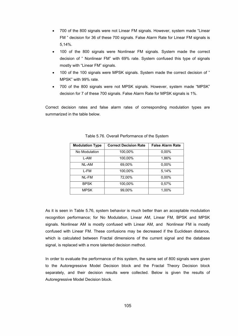
• 700 of the 800 signals were not Linear FM signals. However, system made “Linear
FM ” decision for 36 of these 700 signals. False Alarm Rate for Linear FM signals is
5,14%.
• 100 of the 800 signals were Nonlinear FM signals. System made the correct
decision of ” Nonlinear FM” with 69% rate. System confused this type of signals
mostly with “Linear FM” signals.
• 100 of the 100 signals were MPSK signals. System made the correct decision of ”
MPSK” with 99% rate.
• 700 of the 800 signals were not MPSK signals. However, system made “MPSK”
decision for 7 of these 700 signals. False Alarm Rate for MPSK signals is 1%.
Correct decision rates and false alarm rates of corresponding modulation types are
summarized in the table below.
Table 5.76. Overall Performance of the System
Modulation Type Correct Decision Rate False Alarm Rate
No Modulation 100,00% 0,00%
L-AM 100,00% 1,86%
NL-AM 69,00% 0,00%
L-FM 100,00% 5,14%
NL-FM 72,00% 0,00%
BPSK 100,00% 0,57%
MPSK 99,00% 1,00%
As it is seen in Table 5.76, system behavior is much better than an acceptable modulation
recognition performance; for No Modulation, Linear AM, Linear FM, BPSK and MPSK
signals. Nonlinear AM is mostly confused with Linear AM, and Nonlinear FM is mostly
confused with Linear FM. These confusions may be decreased if the Euclidean distance,
which is calculated between Fractal dimensions of the current signal and the database
signal, is replaced with a more talented decision method.
In order to evaluate the performance of this system, the same set of 800 signals were given
to the Autoregressive Model Decision block and the Fractal Theory Decision block
separately, and their decision results were collected. Below is given the results of
Autoregressive Model Decision block.
105
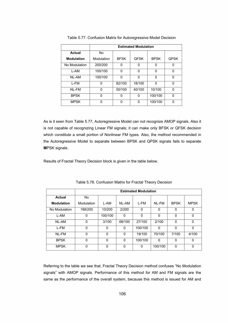
Table 5.77. Confusion Matrix for Autoregressive Model Decision
Estimated Modulation
Actual Modulation
No
Modulation BFSK QFSK BPSK QPSK
No Modulation 200/200 0 0 0 0
L-AM 100/100 0 0 0 0
NL-AM 100/100 0 0 0 0
L-FM 0 82/100 18/100 0 0
NL-FM 0 50/100 40/100 10/100 0
BPSK 0 0 0 100/100 0
MPSK 0 0 0 100/100 0
As is it seen from Table 5.77, Autoregressive Model can not recognize AMOP signals. Also it
is not capable of recognizing Linear FM signals; it can make only BFSK or QFSK decision
which constitute a small portion of Nonlinear FM types. Also, the method recommended in
the Autoregressive Model to separate between BPSK and QPSK signals fails to separate
MPSK signals.
Results of Fractal Theory Decision block is given in the table below.
Table 5.78. Confusion Matrix for Fractal Theory Decision
Estimated Modulation
Actual Modulation
No
Modulation L-AM NL-AM L-FM NL-FM BPSK MPSK
No Modulation 188/200 10/200 2/200 0 0 0 0
L-AM 0 100/100 0 0 0 0 0
NL-AM 0 3/100 68/100 27/100 2/100 0 0
L-FM 0 0 0 100/100 0 0 0
NL-FM 0 0 0 19/100 70/100 7/100 4/100
BPSK 0 0 0 100/100 0 0 0
MPSK 0 0 0 0 100/100 0 0
Referring to the table we see that, Fractal Theory Decision method confuses “No Modulation
signals” with AMOP signals. Performance of this method for AM and FM signals are the
same as the performance of the overall system, because this method is issued for AM and
106

FM recognition in the whole system too. However, Fractal Theory Decision method itself is
not capable of recognizing PSK signals, thus confuses PSK signals with FMOP types.
107
CHAPTER 6
6. CONCLUSIONS In this thesis, the problem of automatic modulation recognition is considered. First of all an
investigation was made in order to understand the reason for radar systems to apply
modulation on their signals. Then a detailed literature search was made among the subject
of Intra-pulse Modulation Recognition. After all, a complete system has been proposed to
recognize the modulation type of IMOP signals.
In this system, benefits of the Auto Regressive Model Decision [8] and Fractal Theory
Decision [7] are combined, and the AM Depth Percent is added as a new feature for more
accurate classification.
The method based on Fractal Theory decision has good performance for CW (no
modulation) and FMOP signals. However during the tests, three main problems are
encountered. The results show that;
- The method fails to distinguish PMOP signals with FMOP signals.
- AMOP signals are mostly confused with FMOP signals.
- The results are sensitive to noise.
This method also cannot classify AM signals. However, being a class of intrapulse
modulations, recognition of AMOP signals is in scope of our work. To overcome this
problem, a new feature as “AM Depth Percent” is inserted to the algorithm. This feature
gives a measure of the modulation on the envelope of the pulse. Together with the “Box
Dimension” and “Information Dimension”, “AM Depth Percent” is used to find the modulation
type of the AMOP signals. However, this requires a pre-knowledge of whether the signal has
FMOP or AMOP property.
To solve this problem, and to be able to recognize PMOP signals, the Autoregressive Model
Decision method is used in corporation with the Fractal Theory Decision method.
The Autoregressive Model Decision method solves the problem of mixing PMOP signals with
FMOP signals. However, the method is not successful for distinguishing between BPSK and
MPSK signals. To overcome this problem, a new decision block is inserted to the system. In
108
this block, magnitudes of the jumps in the phase of the pulse is calculated. Then, if the
minimum magnitude is less than π radians, the signal is decided to have MPSK modulation,
otherwise BPSK modulation. However, for the success of the differentiation method, correct
retrieval of the signal phase from the predetection signal is essential. Correct retrieval of the
signal phase is directly dependent on the accuracy of the estimated center frequency. To
eliminate the effect of the error in estimated center frequency, phase of the signal is
corrected according to the deviation of the extracted Pulse Frequency Mean from the IF.
Furthermore, before all these decision blocks the signal is passed through a bandpass filter
centered on the intermediate frequency. By this way noise is suppressed more and this
improves the system performance for low SNR applications.
Performance tests were made for the resultant system. Same set of signals were input to the
Fractal Theory Decision block and Autoregressive Model Decision block individually. It is
observed that the proposed system shows better performance than the other two systems.
The system we propose shows good performance for SNR values greater than 10-15dB.
Improving system performance for more noisy environments can be considered as a future
work.
Additionally, for AMOP and FMOP signals, we can make Linear or Nonlinear decision for the
last. Decision of the exact modulation shape for these signals can be another future work to
be considered.
As a result, Modulation Recognition solution offered in this thesis collects the beneficial
points of the Autoregressive Model Decision Method and Fractal Theory Decision Method,
and together with the usage of AM Depth Percent value and the IMOP Database, gives a
more comprehensive solution for the “Modulation Recognition of IMOP Signals” problem.
Moreover, if the recognition of Unintentional Modulations on Pulse (UMOP) is also studied,
analysis of IMOP and UMOP signals will introduce a compact solution for the Specific
Emitter Identification (SEI) problem.
109
REFERENCES [1] http://www.geocities.com/jasonlemons/radar/topic2.htm, 18thMay, 2003 [2] Öznur Ateş, “A Survey on Modulation Recognition”, December 2002
[3] D.Boiteau, C.Le Martret, “A General Maximum Likelihood Framework for Modulation
Classification”, 1998 IEEE
[4] Yu-Chuan Lin and C.-C. Jay Kuo, “Sequential Modulation Classification of Dependent
Samples”, 1996 IEEE
[5] Bijan G. Mobasseri, “Digital Modulation Classification Using Constellation Shape”,
November 20, 1997.
[6] Gexiang Zhang, Laizhao Hu, Weidong Jin, “Complexity Feature Extraction of Radar
Emitter Signals”, Asia-Pacific Conference on Environmental Electromagnetics CEEM’2003,
Nov. 4-7, 2003, Hangzhou, China
[7] Gexiang Zhang, Weidong Jin, Laizhao Hu, “Fractal Feature Extraction of Radar Emitter
Signals”, Asia-Pacific Conference on Environmental Electromagnetics CEEM’2003, Nov. 4-7,
2003, Hangzhou, China
[8] Assaleh, K. Farrell, K. Mammone, R.J., “A New Method of Modulation Classification for
Digitally Modulated Signals”, Rutgers Univ., Piscataway, NJ; This paper appears in: Military
Communications Conference, 1992. MILCOM '92, Conference Record. 'Communications -
Fusing Command, Control and Intelligence'., IEEE; Meeting Date: 10/11/1992 -10/14/1992;
Publication Date: 11-14 Oct 1992
[9] Oldřich Zmeškal, Michal Veselý, Martin Nežádal, Miroslav Buchníček, “Fractal Analysis of
Image Structures”, Institute of Physical and Applied Chemistry, Brno University of
Technology, Purkynova 118, 612 00 Brno, Czech Republic
[10] Timo Dickscheid, “Estimating Fractal Dimension; Some Approaches used in Image
Processing”, 30th November 2004.
[11] Bassem R.Mahafza, Ph.D., “Radar Systems Analysis and Design Using Matlab”,
COLSA Corporation, Huntsville, Alabama, 2000.
[12] Simon Haykin, “Communication Systems”, John Wiley, 1994
110

[13] Alan V. Oppenheim and Ronald W. Schafer, “Discrete-Time Signal Processing”,
Prentice Hall, 1986
[14] Gardner, W. A., 1994: “Cyclostationarity in Communications and Signal Processing”,
IEEE Press, 504pp
111

APPENDICES
A. MODULATION SHAPES
AMPLITUDE MODULATION SHAPES
Amplitude, Frequency and Phase components and the baseband signal corresponding to
AM shapes which are considered in this thesis are illustrated in the figures below.
112

1 1.5 2 2.5 3 3.5 4
x 104
0
0.005
0.01
Amplitude
1 1.5 2 2.5 3 3.5 4
x 104
-1
-0.5
0
0.5
1x 10
4 Frequency
1 1.5 2 2.5 3 3.5 4
x 104
-5
0
5
Phase
1 1.5 2 2.5 3 3.5 4
x 104
-0.01
-0.005
0
0.005
0.01
Baseband Signal
Figure A.1. Linear Increasing Amplitude Modulation (PW = 100µsec, Fs = 320kHz, AM
Depth = 50%)
113

1 1.5 2 2.5 3 3.5 4
x 104
0
0.005
0.01
Amplitude
1 1.5 2 2.5 3 3.5 4
x 104
-1
-0.5
0
0.5
1x 10
4 Frequency
1 1.5 2 2.5 3 3.5 4
x 104
-5
0
5
Phase
1 1.5 2 2.5 3 3.5 4
x 104
-0.01
-0.005
0
0.005
0.01
Baseband Signal
Figure A.2. Linear Decreasing Amplitude Modulation (PW = 100µsec, Fs = 320kHz, AM
Depth = 50%)
114

1 1.5 2 2.5 3 3.5 4
x 104
0
0.005
0.01
Amplitude
1 1.5 2 2.5 3 3.5 4
x 104
-1
-0.5
0
0.5
1x 10
4 Frequency
1 1.5 2 2.5 3 3.5 4
x 104
-5
0
5
Phase
1 1.5 2 2.5 3 3.5 4
x 104
-0.01
-0.005
0
0.005
0.01
Baseband Signal
Figure A.3. Positive Parabolic Amplitude Modulation (PW = 100µsec, Fs = 320kHz, AM
Depth = 50%)
115
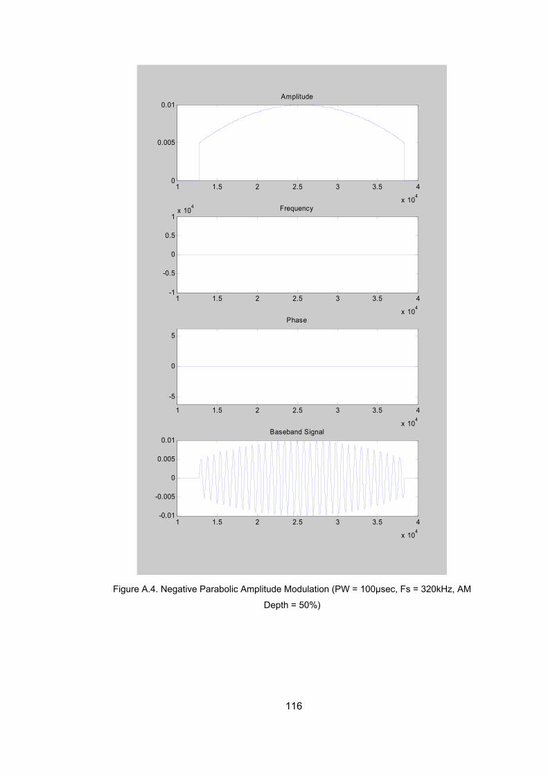
1 1.5 2 2.5 3 3.5 4
x 104
0
0.005
0.01Amplitude
1 1.5 2 2.5 3 3.5 4
x 104
-1
-0.5
0
0.5
1x 10
4 Frequency
1 1.5 2 2.5 3 3.5 4
x 104
-5
0
5
Phase
1 1.5 2 2.5 3 3.5 4
x 104
-0.01
-0.005
0
0.005
0.01Baseband Signal
Figure A.4. Negative Parabolic Amplitude Modulation (PW = 100µsec, Fs = 320kHz, AM
Depth = 50%)
116

1 1.5 2 2.5 3 3.5 4
x 104
0
0.005
0.01
Amplitude
1 1.5 2 2.5 3 3.5 4
x 104
-1
-0.5
0
0.5
1x 10
4 Frequency
1 1.5 2 2.5 3 3.5 4
x 104
-5
0
5
Phase
1 1.5 2 2.5 3 3.5 4
x 104
-0.01
-0.005
0
0.005
0.01
Baseband Signal
Figure A.5. Sinusoidal Amplitude Modulation (PW = 100µsec, Fs = 320kHz, AM Depth =
50%)
117

1 1.5 2 2.5 3 3.5 4
x 104
0
0.005
0.01
Amplitude
1 1.5 2 2.5 3 3.5 4
x 104
-1
-0.5
0
0.5
1x 10
4 Frequency
1 1.5 2 2.5 3 3.5 4
x 104
-5
0
5
Phase
1 1.5 2 2.5 3 3.5 4
x 104
-0.01
-0.005
0
0.005
0.01
Baseband Signal
Figure A.6. Triangular Amplitude Modulation (PW = 100µsec, Fs = 320kHz, AM Depth =
50%)
118
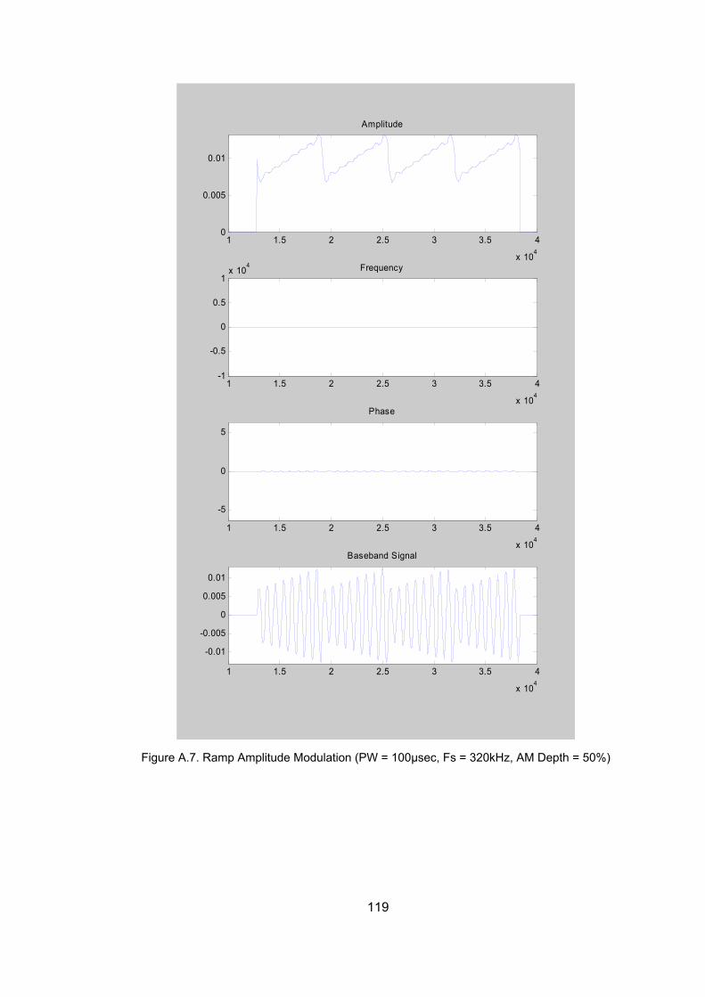
1 1.5 2 2.5 3 3.5 4
x 104
0
0.005
0.01
Amplitude
1 1.5 2 2.5 3 3.5 4
x 104
-1
-0.5
0
0.5
1x 10
4 Frequency
1 1.5 2 2.5 3 3.5 4
x 104
-5
0
5
Phase
1 1.5 2 2.5 3 3.5 4
x 104
-0.01
-0.005
0
0.005
0.01
Baseband Signal
Figure A.7. Ramp Amplitude Modulation (PW = 100µsec, Fs = 320kHz, AM Depth = 50%)
119
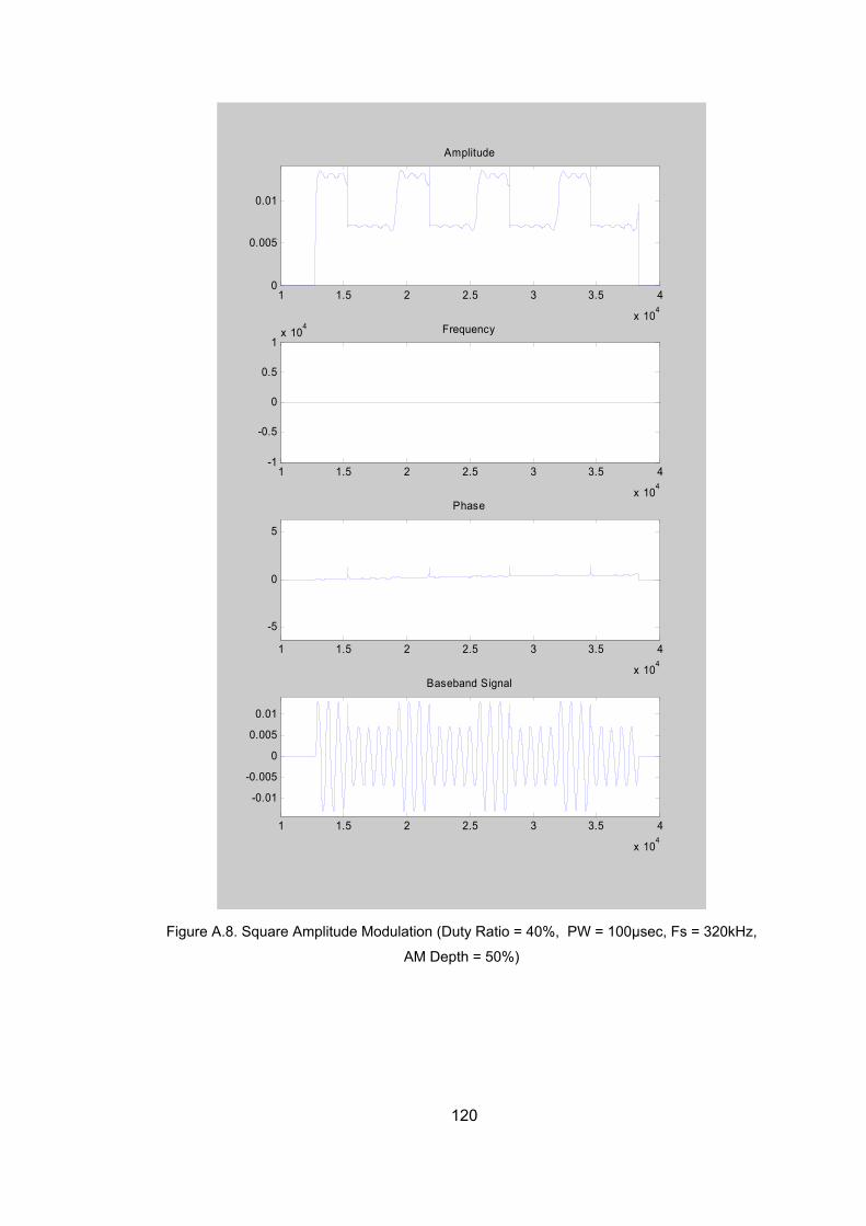
1 1.5 2 2.5 3 3.5 4
x 104
0
0.005
0.01
Amplitude
1 1.5 2 2.5 3 3.5 4
x 104
-1
-0.5
0
0.5
1x 10
4 Frequency
1 1.5 2 2.5 3 3.5 4
x 104
-5
0
5
Phase
1 1.5 2 2.5 3 3.5 4
x 104
-0.01
-0.005
0
0.005
0.01
Baseband Signal
Figure A.8. Square Amplitude Modulation (Duty Ratio = 40%, PW = 100µsec, Fs = 320kHz,
AM Depth = 50%)
120

FREQUENCY MODULATION SHAPES
Amplitude, Frequency and Phase components and the baseband signal corresponding to
FM shapes which are considered in this thesis are illustrated in the figures below
121
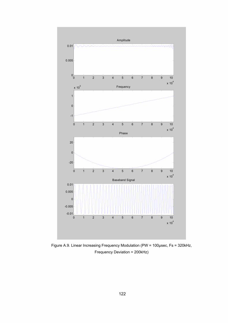
0 1 2 3 4 5 6 7 8 9 10
x 104
0
0.005
0.01
Amplitude
0 1 2 3 4 5 6 7 8 9 10
x 104
-1
0
1
x 105 Frequency
0 1 2 3 4 5 6 7 8 9 10
x 104
-20
0
20
Phase
0 1 2 3 4 5 6 7 8 9 10
x 104
-0.01
-0.005
0
0.005
0.01Baseband Signal
Figure A.9. Linear Increasing Frequency Modulation (PW = 100µsec, Fs = 320kHz,
Frequency Deviation = 200kHz)
122
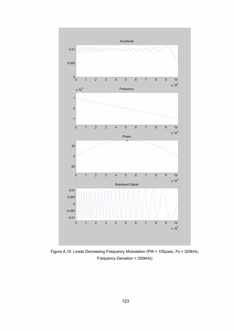
0 1 2 3 4 5 6 7 8 9 10
x 104
0
0.005
0.01
Amplitude
0 1 2 3 4 5 6 7 8 9 10
x 104
-1
0
1
x 105 Frequency
0 1 2 3 4 5 6 7 8 9 10
x 104
-20
0
20
Phase
0 1 2 3 4 5 6 7 8 9 10
x 104
-0.01
-0.005
0
0.005
0.01
Baseband Signal
Figure A.10. Linear Decreasing Frequency Modulation (PW = 100µsec, Fs = 320kHz,
Frequency Deviation = 200kHz)
123

0 1 2 3 4 5 6 7 8 9 10
x 104
0
0.005
0.01
Amplitude
0 1 2 3 4 5 6 7 8 9 10
x 104
-1
0
1
x 105 Frequency
0 1 2 3 4 5 6 7 8 9 10
x 104
-20
0
20
Phase
0 1 2 3 4 5 6 7 8 9 10
x 104
-0.01
-0.005
0
0.005
0.01Baseband Signal
Figure A.11. Positive Parabolic Frequency Modulation (PW = 100µsec, Fs = 320kHz,
Frequency Deviation = 100kHz)
124
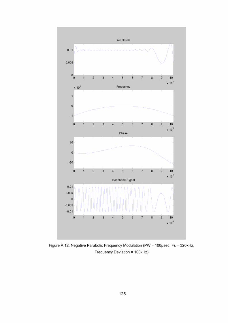
0 1 2 3 4 5 6 7 8 9 10
x 104
0
0.005
0.01
Amplitude
0 1 2 3 4 5 6 7 8 9 10
x 104
-1
0
1
x 105 Frequency
0 1 2 3 4 5 6 7 8 9 10
x 104
-20
0
20
Phase
0 1 2 3 4 5 6 7 8 9 10
x 104
-0.01
-0.005
0
0.005
0.01
Baseband Signal
Figure A.12. Negative Parabolic Frequency Modulation (PW = 100µsec, Fs = 320kHz,
Frequency Deviation = 100kHz)
125

0 1 2 3 4 5 6 7 8 9 10
x 104
0
0.005
0.01
Amplitude
0 1 2 3 4 5 6 7 8 9 10
x 104
-1
0
1
x 105 Frequency
0 1 2 3 4 5 6 7 8 9 10
x 104
-20
0
20
Phase
0 1 2 3 4 5 6 7 8 9 10
x 104
-0.01
-0.005
0
0.005
0.01
Baseband Signal
Figure A.13. Sinusoidal Frequency Modulation (PW = 100µsec, Fs = 320kHz, Frequency
Deviation = 100kHz)
126

0 1 2 3 4 5 6 7 8 9 10
x 104
0
0.005
0.01
Amplitude
0 1 2 3 4 5 6 7 8 9 10
x 104
-1
0
1
x 105 Frequency
0 1 2 3 4 5 6 7 8 9 10
x 104
-60
-40
-20
0
20
Phase
0 1 2 3 4 5 6 7 8 9 10
x 104
-0.01
-0.005
0
0.005
0.01
Baseband Signal
Figure A.14. Triangular Frequency Modulation (PW = 100µsec, Fs = 320kHz, Frequency
Deviation = 100kHz)
127

0 1 2 3 4 5 6 7 8 9 10
x 104
0
0.01
0.02
0.03
0.04
Amplitude
0 1 2 3 4 5 6 7 8 9 10
x 104
-1
0
1
x 105 Frequency
0 1 2 3 4 5 6 7 8 9 10
x 104
-60
-40
-20
0
20
Phase
0 1 2 3 4 5 6 7 8 9 10
x 104
-0.04
-0.02
0
0.02
0.04Baseband Signal
Figure A.15. Ramp Frequency Modulation (PW = 100µsec, Fs = 320kHz, Frequency
Deviation = 100kHz)
128

0 1 2 3 4 5 6 7 8 9 10
x 104
0
0.01
0.02
0.03
0.04
Amplitude
0 1 2 3 4 5 6 7 8 9 10
x 104
-1
0
1
x 105 Frequency
0 1 2 3 4 5 6 7 8 9 10
x 104
-10
0
10
20
Phase
0 1 2 3 4 5 6 7 8 9 10
x 104
-0.04
-0.02
0
0.02
0.04
Baseband Signal
Figure A.16. Square Frequency Modulation (PW = 100µsec, Fs = 320kHz, Frequency
Deviation = 100kHz, Duty Ratio = 40%)
129
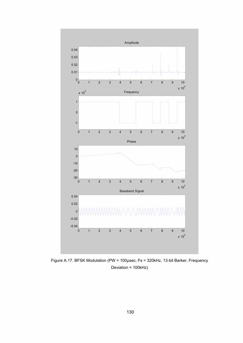
130
0 1 2 3 4 5 6 7 8 9 10
x 104
0
0.01
0.02
0.03
0.04
Amplitude
0 1 2 3 4 5 6 7 8 9 10
x 104
-1
0
1
x 105 Frequency
0 1 2 3 4 5 6 7 8 9 10
x 104
-30
-20
-10
0
10
Phase
0 1 2 3 4 5 6 7 8 9 10
x 104
-0.04
-0.02
0
0.02
0.04
Baseband Signal
Figure A.17. BFSK Modulation (PW = 100µsec, Fs = 320kHz, 13-bit Barker, Frequency
Deviation = 100kHz)

131
PHASE MODULATION SHAPES
Amplitude, Frequency and Phase components and the baseband signal corresponding to
PM shapes which are examples of the modulation shapes considered in this thesis are
illustrated in the figures below

132
1 1.5 2 2.5 3 3.5 4
x 104
0
0.01
0.02
0.03
Amplitude
1 1.5 2 2.5 3 3.5 4
x 104
-0.2
0
0.2
0.4
0.6Frequency
1 1.5 2 2.5 3 3.5 4
x 104
-5
0
5
Phase
1 1.5 2 2.5 3 3.5 4
x 104
-0.02
0
0.02
Baseband Signal
Figure A.18. BPSK Modulation (PW = 100µsec, Fs = 320kHz, 13-bit Barker)
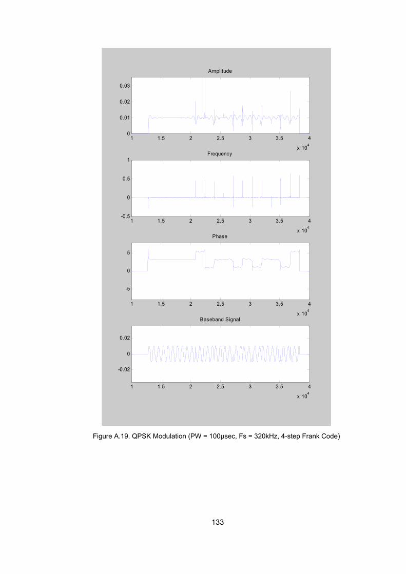
133
1 1.5 2 2.5 3 3.5 4
x 104
0
0.01
0.02
0.03
Amplitude
1 1.5 2 2.5 3 3.5 4
x 104
-0.5
0
0.5
1Frequency
1 1.5 2 2.5 3 3.5 4
x 104
-5
0
5
Phase
1 1.5 2 2.5 3 3.5 4
x 104
-0.02
0
0.02
Baseband Signal
Figure A.19. QPSK Modulation (PW = 100µsec, Fs = 320kHz, 4-step Frank Code)
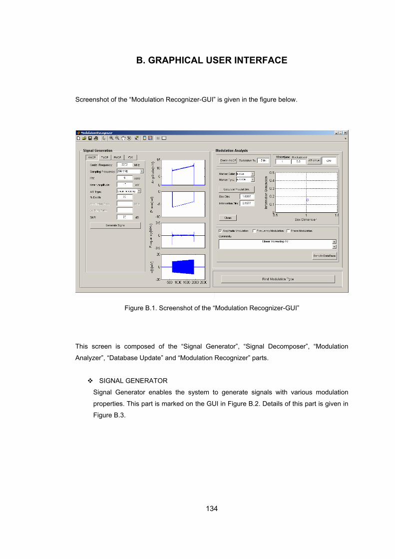
134
B. GRAPHICAL USER INTERFACE Screenshot of the “Modulation Recognizer-GUI” is given in the figure below.
Figure B.1. Screenshot of the “Modulation Recognizer-GUI”
This screen is composed of the “Signal Generator”, “Signal Decomposer”, “Modulation
Analyzer”, “Database Update” and “Modulation Recognizer” parts.
SIGNAL GENERATOR
Signal Generator enables the system to generate signals with various modulation
properties. This part is marked on the GUI in Figure B.2. Details of this part is given in
Figure B.3.
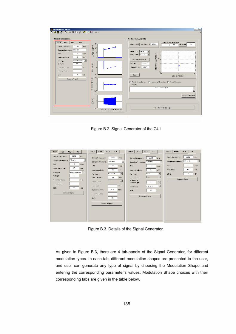
135
Figure B.2. Signal Generator of the GUI
Figure B.3. Details of the Signal Generator.
As given in Figure B.3, there are 4 tab-panels of the Signal Generator, for different
modulation types. In each tab, different modulation shapes are presented to the user,
and user can generate any type of signal by choosing the Modulation Shape and
entering the corresponding parameter’s values. Modulation Shape choices with their
corresponding tabs are given in the table below.
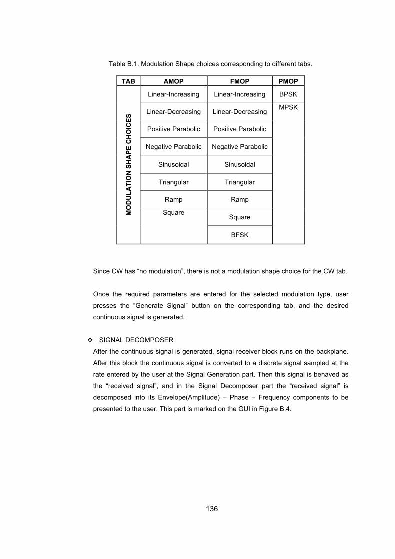
136
Table B.1. Modulation Shape choices corresponding to different tabs.
TAB AMOP FMOP PMOP
Linear-Increasing Linear-Increasing BPSK
Linear-Decreasing Linear-Decreasing
Positive Parabolic Positive Parabolic
Negative Parabolic Negative Parabolic
Sinusoidal Sinusoidal
Triangular Triangular
Ramp Ramp
Square MO
DU
LATI
ON
SH
APE
CH
OIC
ES
Square
BFSK
MPSK
Since CW has “no modulation”, there is not a modulation shape choice for the CW tab.
Once the required parameters are entered for the selected modulation type, user
presses the “Generate Signal” button on the corresponding tab, and the desired
continuous signal is generated.
SIGNAL DECOMPOSER
After the continuous signal is generated, signal receiver block runs on the backplane.
After this block the continuous signal is converted to a discrete signal sampled at the
rate entered by the user at the Signal Generation part. Then this signal is behaved as
the “received signal”, and in the Signal Decomposer part the “received signal” is
decomposed into its Envelope(Amplitude) – Phase – Frequency components to be
presented to the user. This part is marked on the GUI in Figure B.4.
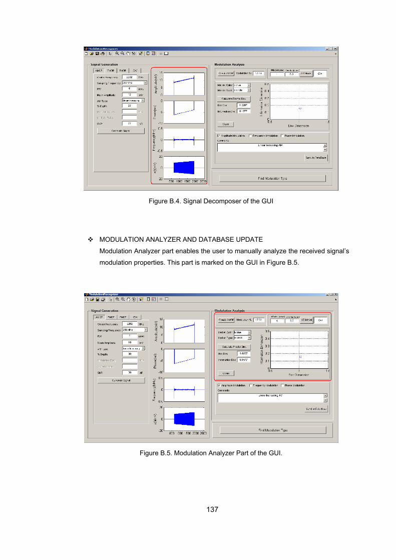
137
Figure B.4. Signal Decomposer of the GUI
MODULATION ANALYZER AND DATABASE UPDATE
Modulation Analyzer part enables the user to manually analyze the received signal’s
modulation properties. This part is marked on the GUI in Figure B.5.
Figure B.5. Modulation Analyzer Part of the GUI.
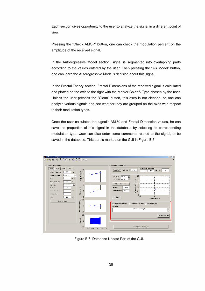
138
Each section gives opportunity to the user to analyze the signal in a different point of
view.
Pressing the “Check AMOP” button, one can check the modulation percent on the
amplitude of the received signal.
In the Autoregressive Model section, signal is segmented into overlapping parts
according to the values entered by the user. Then pressing the “AR Model” button,
one can learn the Autoregressive Model’s decision about this signal.
In the Fractal Theory section, Fractal Dimensions of the received signal is calculated
and plotted on the axis to the right with the Marker Color & Type chosen by the user.
Unless the user presses the “Clean” button, this axes is not cleaned, so one can
analyze various signals and see whether they are grouped on the axes with respect
to their modulation types.
Once the user calculates the signal’s AM % and Fractal Dimension values, he can
save the properties of this signal in the database by selecting its corresponding
modulation type. User can also enter some comments related to the signal, to be
saved in the database. This part is marked on the GUI in Figure B.6.
Figure B.6. Database Update Part of the GUI.
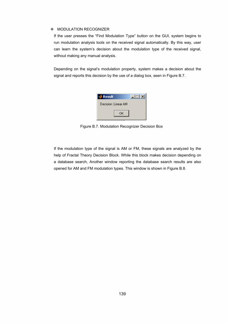
139
MODULATION RECOGNIZER
If the user presses the “Find Modulation Type” button on the GUI, system begins to
run modulation analysis tools on the received signal automatically. By this way, user
can learn the system’s decision about the modulation type of the received signal,
without making any manual analysis.
Depending on the signal’s modulation property, system makes a decision about the
signal and reports this decision by the use of a dialog box, seen in Figure B.7.
Figure B.7. Modulation Recognizer Decision Box
If the modulation type of the signal is AM or FM, these signals are analyzed by the
help of Fractal Theory Decision Block. While this block makes decision depending on
a database search, Another window reporting the database search results are also
opened for AM and FM modulation types. This window is shown in Figure B.8.
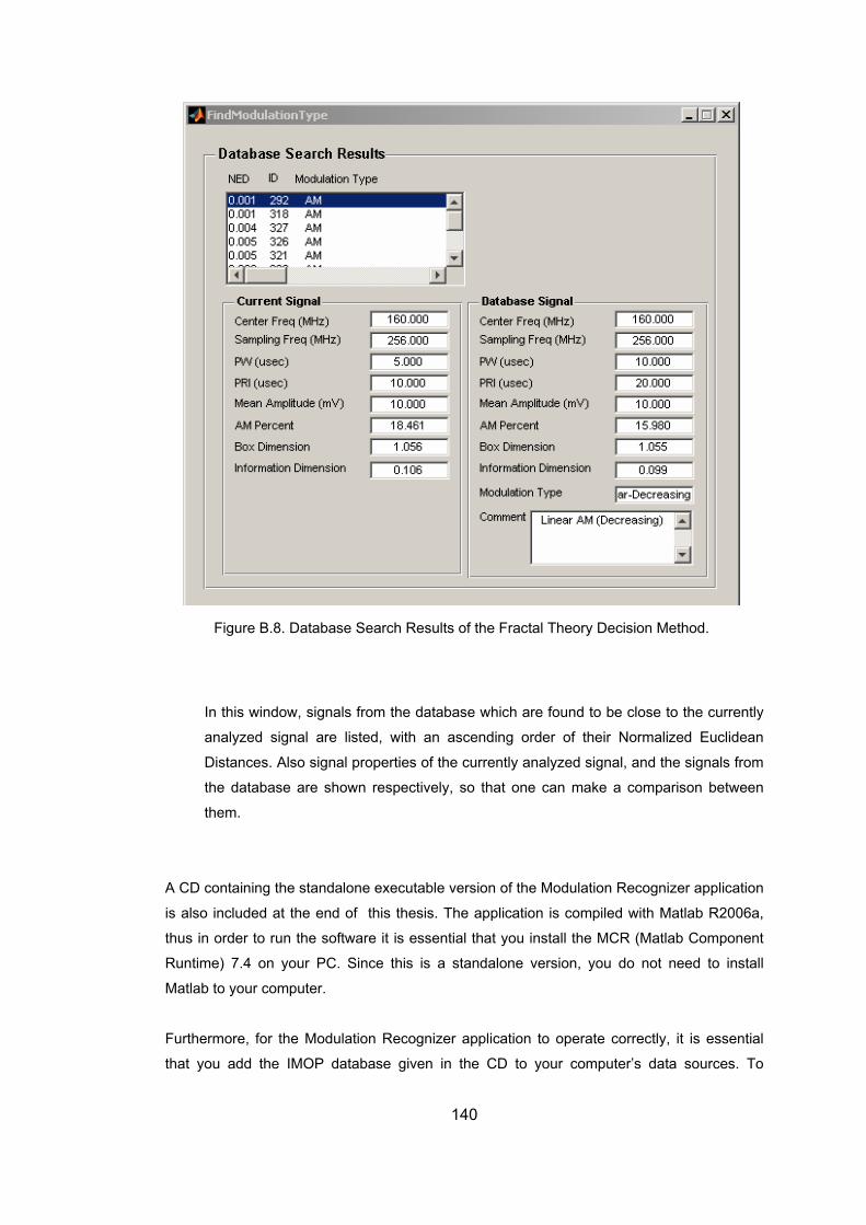
140
Figure B.8. Database Search Results of the Fractal Theory Decision Method.
In this window, signals from the database which are found to be close to the currently
analyzed signal are listed, with an ascending order of their Normalized Euclidean
Distances. Also signal properties of the currently analyzed signal, and the signals from
the database are shown respectively, so that one can make a comparison between
them.
A CD containing the standalone executable version of the Modulation Recognizer application
is also included at the end of this thesis. The application is compiled with Matlab R2006a,
thus in order to run the software it is essential that you install the MCR (Matlab Component
Runtime) 7.4 on your PC. Since this is a standalone version, you do not need to install
Matlab to your computer.
Furthermore, for the Modulation Recognizer application to operate correctly, it is essential
that you add the IMOP database given in the CD to your computer’s data sources. To
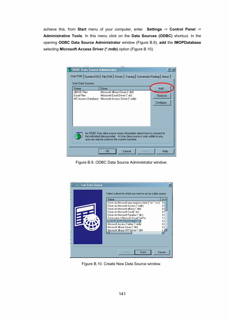
141
achieve this, from Start menu of your computer, enter Settings -> Control Panel ->
Administrative Tools. In this menu click on the Data Sources (ODBC) shortcut. In the
opening ODBC Data Source Administrator window (Figure B.9), add the IMOPDatabase selecting Microsoft Access Driver (*.mdb) option (Figure B.10).
Figure B.9. ODBC Data Source Administrator window.
Figure B.10. Create New Data Source window.
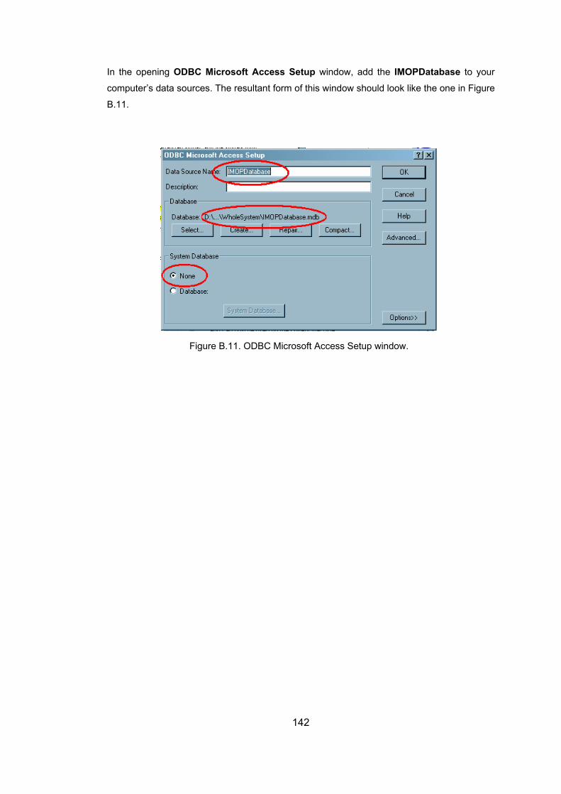
142
In the opening ODBC Microsoft Access Setup window, add the IMOPDatabase to your
computer’s data sources. The resultant form of this window should look like the one in Figure
B.11.
Figure B.11. ODBC Microsoft Access Setup window.
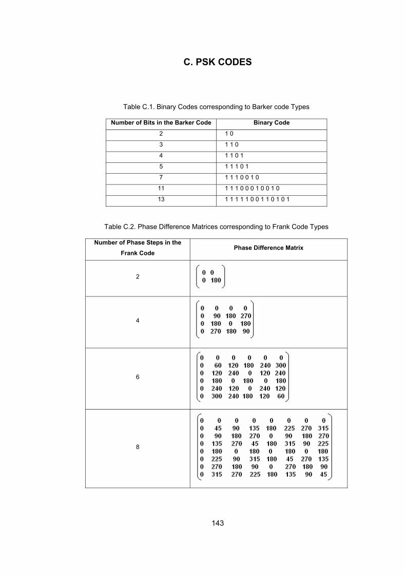
143
C. PSK CODES
Table C.1. Binary Codes corresponding to Barker code Types
Number of Bits in the Barker Code Binary Code
2 1 0
3 1 1 0
4 1 1 0 1
5 1 1 1 0 1
7 1 1 1 0 0 1 0
11 1 1 1 0 0 0 1 0 0 1 0
13 1 1 1 1 1 0 0 1 1 0 1 0 1
Table C.2. Phase Difference Matrices corresponding to Frank Code Types
Number of Phase Steps in the Frank Code
Phase Difference Matrix
2
4
6
8