'¢e "~) I t, ,

AD-A237 635III hllil i t 11 _

U ~'U Defence wn.1onale

MODULATION RECOGNITION:AN OVERVIEW

by

Rene Lamontagne

91-04406111 11 I I 111111 I l I

DEFENCE RESEARCH ESTABLISHMENT OTTAWATECHNICAL NOTE 91-3

11 ~ March 1991,;! I ,Il ;!Ottaw,i

*~.ENata Dd -

EWE De,,nc. national.

* 2'

ist i

MODULATION RECOGNITION:AN OVERVIEW

by

Rene' LamontagneCommunications Electronic Warfare Sectiao

Electronic Warfare Division

DEFENCE RESEARCH ESTABLISHMENT OTTAWATECHNICAL NOTE 91-3

PCN March 1991041LK11 Ottawa

ABSTRACT

"vhe interest for a system able to automatically identify the modulation type of anintercepted radio signal is increasingly evident for military and civilian purposes. Althoughin the past some authors looked at the problem, nobody found "the solution" and theproblem remains. Therefore, an overview of the proposed techniques is useful in order toassess the actual situation.

This document presents classification techniques and featires (parameterscharacterizing the modulation types) used for modulation recognition.

RESUME

Que ce soit pour des fins militaires ou civiles, l'int6rdt d'une machine capabled'identifier automatiquement le type de modulation d'un signal inconnu est 6vident. Bienquo par le pass6 certains auteurs se soient pench~s sur le probl~me, personne n'a obtenued'6clatant r~sultats indiquant la route . suivre. Par consequent il n'y a pas lieu deconcentrer ses efforts sur un seul auteur mais sur l'ensemble des techniques proposees.

Ce document couvre donc le sujet d'une fagon globale, pr~sentant les techniquespour classification ainsi que les param~tres utilis6s pour caract6riser et distinguer les diverstypes de modulation, tel que propos6s par les auteurs.

°oI

EXECUTIVE SUMMARY

The motivation of this document is the interest of military and civilianorganisations in monitoring the electromagnetic signal activity in the RF spectrum. Sincethe number of competent trained human operators is constantly decreasing and the radioactivity in the HF and VHF bands increasing, the interest of a machine capable ofautomatically identifying the modulation type of an unknown intercepted signal is quiteobvious. Integrating this device into an ESM system including energy detection (spectralanalysis) Direction Finding and Data Fusion and Correlation, would allow an operator todrastically improve his efficiency and his ability to monitor the activity in the RFspectrum.

Although in the past some authors looked at the problem and proposed algorithmspermitting to achieve proper performance for high SOR signals, for an ESM perspective lowSNR signals are more likely to be intercepted. Therefore, the problem of finding goodparameters able to discriminate among the modulation types of interest when the noise isimportant, still remains and is very realistic. More and more publications appear in theliterature presenting new ideas and better performance. Also, with the appearance ofbetter hardware processors, new possibilities are now available and it is believed that soona modulation recognition device will be able to classify very noisy signals in a short periodof time with a high accuracy. Although such a device is not yet available, the work doneuntil now is certainly worthy and merits consideration.

This document introduces and presents techniques proposed in the open literaturefor automatic modulation type identification of an intercepted radio signal. Most of thesetechniques are baspd on the same classic pattern recognition theory, which is presented in aseparate section, since it is a prerequisite to understand the following sections. The twomain classification techniques used for modulation recognition, the linear classifier and thedecision tree, are more specifically discussed.

Modulation recognition is concerned with analog as well as digital modulation types.Although there is a modern tendency to replace analog modulation types by digital ones,analog modulations (i.e., SSB, FM, AM, etc.) are still in use in many countries. Themotivation to intercept these signals is reinforced by the fact that these signals, onceidentified, can also be demodulated to extract the message. It might not be the case withdigital modulation types, since usually coding is involved: error correcting code,encryption, vocoder, etc.

Since the main differences between the approaches proposed by the referred authorsare the features they used, the main part of the document consists in presenting thesefeatures and the corresponding results. Also, more particular points are considered such aspreprocessing to remove gaps in analog amplitude modulated signals.

The purpose of this technical note is to summarize in a very comprehensive way allthe publications on the topic of modulation recognition.

v

CONTENTS

ABSTRACT/RESUME iii

EXECUTIVE SUMMARY v

CONTENTS vii

LIST OF FIGURES xi

LIST OF TABLES xiii

1.0 INTRODUCTION 1

2.0 CLASSIFICATION TECHNIQUES 6

2.1 GENERAL 62.2 PATTERN RECOGNITION TECHNIQUES 7

2.2.1 Feature Selection 92.2.2 Feature Extraction 112.2.3 Classification Techniques 12

2.2.3.1 Linear Classifiers 122.2.3.2 Decision Tree Classifiers 15

2.3 MODULATION RECOGNITION 16

3.0 MR FOR ANALOG MODULATIONS 20

3.1 MILLER APPROACH 203.1.1 Miller 203.1.2 Wakeman 233.1.3 Fry 23

3.2 GADBOIS APPROACH 233.2.1 Gadbois 233.2.2 Ribble 263.2.3 UTL 273.2.4 Gallant 27

3.3 OTHER APPROACHES 313.3.1 Weaver 313.3.2 Winkler 313.3.3 Callaghan 313.3.4 Fabrizi 313.3.5 Petrovic 33

3.4 AISBETT APPROACH 343.4.1 Aisbett 343.4.2 Einicke 35

3.5 HIPP APPROACH 363.5.1 Hipp 36

vii

4.0 MR FOR DIGITAL MODULATIONS 38

4.1 LIEDTKE AND JONDRAL APPROACH 384.1.1 Liedtke 384.1.2 Jondral 424.1.3 Dominguez 444.1.4 Adams 45

4.2 OTHER APPROACHES 454.2.1 Mammone 454.2.2 DeSimio 46

5.0 MR BASED ON ENERGY DETECTION ALGORITHMS 48

5.1 READY APPROACH 485.2 KIM APPROACH 505.3 GARDNER APPROACH 51

6.0 CONCLUSION 53

REFERENCES REF-1

ix

LIST OF FIGURES

Figure Page

1 Informational Relationships 22 Example of a simple ESM system 33 The two major phases for pattern classifier

development 84 Dimensionality reduction by feature extraction-

selection 85 Distribution of the feature for the two classes 106 Decision Region: 2 features and 2 classes 107 Cluster shapes possible (tvo classes) 148 General architecture of a MR system 169 Illustration of the logic tree decision process 1710 Millei's classifier 2111 Theorical APDs 2112 Mathematical relations relating R to the SNR 2413 Gadbois' system block diagram 2514 Ribble's system block diagram 2615 Experiment block diagram 2816 Variance of R diminished by preprocessing 2917 The new feature VAR proposed by Gallant 3018 Fabrizi's features 3219 Fabrizi's Decision Tree 3220 Petrovic's classifier 3321 Distributions of Aisbett's parameter A20' and

the typical parameter A. 3422 Block diagram of Liedtke's classifier 3923 Liedtke's universal demodulator 3924 Classification of PSK signals by Liedtke 4025 Schematized class space with separation parameters 4126 Liedtke's results 4227 Examples of histograms 4328 Intercepted spectrum 4429 A single unit of the perceptron classifier 4730 One of 3 similar stages of Ready's system 4831 Example of the processing performed by the system 4932 Theorical spectral correlation distributions 52

x

LIST OF TABLES

Table

1 Groups of authors 192 Miller's Reference Logic Table 223 Gadbois' confusion table 244 Features evaluated by Hipp 365 Mammone's results 466 Examples of features used for modulation

recognition 54

xiii

1.0 INTRODUCTION

From the earliest days of radio communication the need to monitor theelectromagnetic signal activity in the RF spectrum has existed. Civilian authorities maywish to monitor the transmissions over their territory in order to maintain a control overthis activity. Military organizations may wish to monitor the radio activiies of otherpowers for reasons, among others, of national security.

Typically, the technique employed by monitoring stations throughout the world isbased upon a well-tried method which has been in use for many years. This is a oneman-one receiver situation in which the operator spends his time searching the RFspectrum with a continuously tunable general purpose receiver, hoping to make aninteresting interception. There are variations to that scenario. For example, it is possibleand common practice for an operator to have two receivers. One is used for searching,w.ile the second remains tuned to a known interesting frequency. A further variation iscaied the master-slave technique. In this method a group of operators is involved. Themaster operates a fast tuning-sweep receiver with an associated panoramic display unit.When a signal of interest is located, this intercepted signal is transferred to one of theslaves, who tunes to the appropriate frequency and does the monitoring with aconventional, general purpose, continuously tunable receiver.

Neither of these techniques overcomes the fundamental problem of seriousovercrowding in the radio spectrum. Moreover, the existing pool of highly skilled operatorshas begun to dry up and it is proving difficult to find replacements (1]. The classicalmethod of monitoring is after all, a very boring occupation. Therefore Electronic SupportMeasure (ESM) techniques become an important alternative.

In advanced ESM systems, the operator is helped or replaced by sophisticatedelectronic machines. These machines are concerned with exploiting enemy electromagneticemissions for the purpose of gathering intelligence information as automatically as possible.This infQrmation is provided by analysis of the attributes of an intercepted signal. Thus,Modulation Recognition (MR) is an ESM technique: given an intercepted signal, it aims toidentify the modulation type among a number of known possible modulation types. Theterms modulation classification, recognition or identification are currently used to describethis process.

Prior to modulation classification, the radio signal must be intercepted, whichmeans that somewhere before the modulation classification system, there is an energydetection system looking for electromagnetic emissions in the bandwidth of interest. Oncea signal has been detected, the logical following step is to try to identify this signal. A stepfarther is the demodulation of that signal and then decryption to finally obtain the signalitself.

Thus classification is neither energy detection nor normal signal demodulation withmessage extraction; it is something in between (see Figure 1).

Infofaon ,,,

signal

Figure 1: Informational Relationships [2, p.312]

For energy detection, only the bandwidth of interest for the ESM system is known.On the other hand, for demodulation with message extraction, knowledge of the centerfrequency, bandwidth, type of modulation, data rate...parameters is required. The signalclassifier should need only the information given by the energy detection system, i.e. wherethe signal is: center frequency and bandwidth.

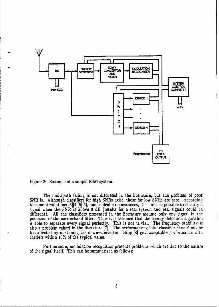
An example of an ESM system is illustrated in Figure 2. The intercepted signal issubmitted to energy detection algorithms, then down-converted and bandpass filtered,prior to modulation recognition. The information obtained from the latter and from theenergy detector is gathered by the system controller, which will assign the signal to aproper demodulator, as shown in Figure 2.

The particular problems related to modulation classification are caused by the radiochannel and the ESM system components. The potential problems could be summarizedby:

Effect Source

-Multipath fading Radio Channel-Poor SNRs Radio Channel-Amplitude distortion Receiver amplifier-More than one signal Energy Detector-Incomplete signal Energy Detector-Frequency instability Down Convertor

2

ENERGY DOWN M ODULATIONRXDETECTOR CONVERTOR RECOG3NISER

AND

"" CONTROL

rom SCC COMPUTER

S DEMOD 1N

TO

ROk~x fd*M Oir, USER

OUTPUT

Figure 2: Example of a simple ESM system.

The multipath fading is not discussed in the literature, but the problem of poorSNR is. Although classifiers for high SNRs exist, those for low SNRs are rare. Accordingto some simulations [3][4][5][6], under ideal circumstances, it uld be possible to classify asignal when the SN is above 8 dB (results for a real sys ii and real signals could b'different). All the classifiers presented in the literature assume only one signal in thepassband of the narrowband filter. Thus it is assumed that the energy detection algorithmis able to separate every signal perfectly. This is not tiLvial. The frequency stability isalso a problem raised in the literature [7]. The performance of the classifier should not betoo affected by mistuning the down-converter. Hipp [8] got acceptable -'"rformance withcarriers within 10% of the typical value.

Furthermore, modulation recognition presents problems which are due to the natureof the signal itself. This can be summarized as follows:

3

Problem Source

-insufficient signal short acquisition time-unmodulated segments gaps in the voice (analog modulations)-long computing time too many features

The performance of a classifier is closely related to the quantity of informationavailable. Thus it is possible to improve the performance of a classifier with longeracquisition times (more sample points) and/or by computing more features from the signal.In both cases the classification process time is increased. The acquisition time is especiallylong for analog modulations. AM, SSB, DSB and FM are afflicted with "unmodulatedsegments" caused by gaps in the voice. These gaps result in CW segments for AM andFM, and in noise segments for SSB and DSB. Gallant [3] presented a technique to removethese unmodulated segments at the r.rice of an acquisition time of at least 1.5 see. Fordigital modulation types, the problem is to get enough symbol transitions, otherwise CWwill be detected. The problem is especially obvious at low data rates. For example, thedata rate of OOK could be as low as 10 Hz, then five seconds are required to get only 50transitions. The effect of the acquisition time on the system performance can be perceivedin [6], [91 and [10].

The computing time depends mainly upon the number of sample points, the numberof extracted features, the number of modulation types, and the complexity of theclassification algorithm. These features permit the user to discriminate among themodulations. More features could provide more discriminating facilities. Also, features areusually time invariant, which means they are computed over all the sample points. Forthese reasons, the features should be easy to compute, so that a reasonable overallcomputing time can be obtained. Also, although some highly sophisticated classificationalgorithms exist, the ones used in pattern recognition are simple. The overall computingtime presented in the literature is about 2 seconds.

In the following sections the process of modulation recognition itself will be treated.Firstly, the concept of classification or recognition will be presented. Although theydescribe the same problem, the term classification and recognition do not represent exactlythe same reality. Recognition (from pattern recognition) includes an additional step beforeclassification: feature extraction and/or selection. This is preparing the data forclassification. Two kinds of classifiers are presented and used for modulation recognition:the linear classifier and the decision tree. They are widely used in real systems becausethey are simple and fast enough for real-time applications. Finally, the researchers in thearea of MR will be summarized in a matrix, in preparation for the next sections whichpresent features used by them in their Modulation Recognition (MR) systems.

Section 3.0 presents MR systems capable of recognizing analog modulation types.The features useful for that purpose are highly sensitive to noise for an obvious reason:analog modulation schemes consist mainly of amplitude modulation (AM, SSB, DSB).However, a few authors presented "less sensitive" features. Another topic introduced inthis section is the problem of gaps in the voice. We will see in detail the interestingsolution proposed by Gallant.

it

The features for digital modulation schemes (Section 4.0) are quite different.Although the separation between Sections 3.0 and 4.0 is very arbitrary (most authors do afew of both), different features are required to be able to get information on the phase ofphase modulated signals (BPSK, QPSK, FSK). These features are given in Section 4.0.

The two preceding sections present features used by pattern recognition algorithmsfor the purpose of modulation recognition. A few authors proposed an alternative way ofdoing MR, by using energy detection algorithms. This perspective is presented in section5.0. Unfortanately, the performance expected from these techniques is not discussed by theauthors.

Finally, Section 6.0 concludes the document with a short summary and comments.

5

2.0 CLASSIFICATION TECHNIQUES

2.1 GENERAL

The term classification is the action of associating individuals into one of two ormore alternative classes (groups) on the basis of a set of inputs called features (variables).The populations are known to be distinct according to the features. As an example,consider an archeologist who wishes to determine which of two possible tribes created aparticular statue found in a dig. The archeologist takes measurements for severalcharacteristics of the statue and decides which tribe these measurements are most likely tohave come from. The measurements of the statue may consist of a single observation suchas its height, however, we would then expect a low degree of accuracy. If on the otherhand the classification is based on several characteristics, we would have more confidencein the prediction.

Classification algorithms could be used in almost any area of knowledge, it is theheart of any decision process. Tou [11] divided problems where classification algorithmsare applied into two major categories:

1. The study of human beings and other living organisms,

2. The development of theory and techniques for the design of devices capable ofperforming a given recognition task for a specific application.

The first subject area is concerned with such disciplines as sociology, psychology,physiology and biomedical sciences. The second area is concerned with computer, andengineering aspects of the design of automatic pattern recognition systems. Patternrecognition can be defined as the categorization of input data into identifiable classes viathe extraction of significant features followed by a classification process. Thus in patternrecognition we are talking of a two step process: feature extraction and classification.Contrary to the preceding examples, in pattern recognitirn there are no direct featuresavailable. Although data is available under a digital form (signal processing ADC), moreprocessing is required to give some meaning to this data. During the feature extractionprocess, the large quantity of data is translated into a few significant and discriminantfeatures used by the classifier.

Pattern recognition spans a number of disciplines and problems, as shown in thefollowing list:

-speech recognition words identification-speaker recognition speaker identification-speaker verification speaker identification

(knowing the words used)-character recognition character identification-visual inspection object anomaly identification-ship recognition kind of ship identification-biomedical analysis medical diagnoses-weather prediction weather forecast--stock market prediction predicted market ups and downs

6

Early pattern recognition researc performed in the '60s and '70s focused on theasymptotic (infinite training data) properties of classifiers. Many researchers studiedparametric Bayesian classifiers, where the form of input distributions is assumed to beknown, and parameters of distributions are estimated using techniques that requiresimultaneous access to all training data. These classifiers, especially those that assumeGaussian distributions, are still the most widely used because they are simple anddescribed in a number of textbooks.

The thrust of recent research has changed, much of it motivated by the desire tounderstand and build parallel neural net classifiers inspired by biological neural networks.This has led to an emphasis on robust, adaptive, non-parametric classifiers that can beimplemented on parallel hardware. It is very likely that future modulation recognitionsystems will use this new technology.

In this chapter, some classical classification techniques will be presented. Thesetechniques are used in pattern recognition as well as in human sciences. The concept offeature extraction and selection will also be introduced. Then the particular problem ofMR itself will be presented.

2.2 PATTERN RECOGNITION TECHNIQUES

The goal of pattern recognition is to assign input patterns to one of k classes. Theinput patterns consist of static input vectors z containing n elements (continuous ordiscrete values) denoted zi, z2, z3,..., z,. These elements represent measurements of featuresselected to be useful for distinguishing between classes and insensitive to irrelevantvariability in the input. A good classification performance requires the selection ofeffective features as well as the selection of a classifier that can make good use of thosefeatures with limited training data, memory, and computing power. During the trainingphase, a limited amount of training data and a priori knowledge concerning the expectedoutput is used to adjust parameters and/or learn the structure of the classifier. Once thetraining is accomplished, the classifier is ready for the test phase, during which a new set ofinputs is presented to the classifier without a priori knowledge (see Figure 3). Theperformance is then computed and presented, usually in a confusion table (percentage ofgood classification for each class).

The subject of feature selection and extraction is concerned with reducing thedimensionality of pattern representation. Since the complexity of a classifier grows rapidlywith the number of dimensions of the pattern space, it is important to base decisions onlyon the most essential, so-called discriminatory information. Dimensionality reduction isalso recommended from a classification performance point of view. Iritially performanceimproves as new features are added, but at some point, inclusion of further features willresult in performance degradation.

Dimensionality reduction can be achieved in two different ways. One approach is toidentify measurements which do not contribute significantly to class separability, this isfeature selection. The other approach, called feature extraction, consists of mapping theuseful information in a lower-dimension feature space (see Figure 4).

7

TRAINING3 PHASE

ADJUST(TRAI~NG~L~J CLASSIFIER PARAMETERS\DATA.~# 1 ANDIOR STRUCTURE

TEST PHASE

CLASSIFICATIONINmTALLY USES DES~IN DECISIONFROM TRAINING PHASE.THNADAPTS TO TEST DATA

Figure 3: The two major phases for pattern classifier development[12, p.48]

CLSIFE DECISION

SESR ,CLASSIFIER DCSO

Dimensionality reduction by feature etrction

Figure 4.D iisoa yrdcinb etr xtrcinslcin

YZ8

To solve a feature selection and/or feature extraction problem, we need some sort ofevaluation criterion. Unfortunately this is not a trivial problem. The quality of a set offeatures is very closely related to the classifier used. Therefore the optimal procedure is totry all the possible sets of features with the classifier and to retain the "best" set. Ingeneral this process requires too much computation and therefore a number of alternativeeat.-re evaluation criteria exist.

It is not the purpose of this document to explain the details of feature evaluationcriteria, however the basic idea will be given in Sections 2.2.1 and 2.2.2.

2.2.1 Feature Selection

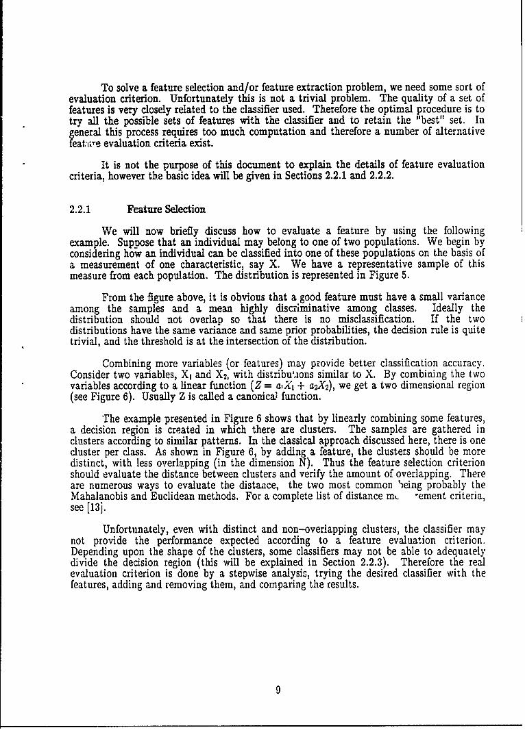
We will now briefly discuss how to evaluate a feature by using the followingexample. Suppose that an individual may belong to one of two populations. We begin byconsidering how an individual can be classified into one of these populations on the basis ofa measurement of one characteristic, say X. We have a representative sample of thismeasure from each population. The distribution is represented in Figure 5.

From the figure above, it is obvious that a good feature must have a small varianceamong the samples and a mean highly discriminative among classes. Ideally thedistribution should not overlap so that there is no misclassification. If the twodistributions have the same variance and same prior probabilities, the decision rule is quitetrivial, and the threshold is at the intersection of the distribution.

Combining more variables (or features) may provide better classification accuracy.Consider two variables, X, and X2, with distribulions similar to X. By combining the twovariables according to a linear function (Z = aX + a2X2), we get a two dimensional region(see Figure 6). Usually Z is called a canonical function.

The example presented in Figure 6 shows that by linearly combining some features,a decision region is created in which there are clusters. The samples are gathered inclusters according to similar patterns. In the classical approach discussed here, there is onecluster per class. As shown in Figure 6, by adding a feature, the clusters should be moredistinct, with less overlapping (in the dimension N). Thus the feature selection criterionshould evaluate the distance between clusters and verify the amount of overlapping. Thereare numerous ways to evaluate the distaace, the two most common 1eing probably theMahalanobis and Euclidean methods. For a complete list of distance m- -ement criteria,see [13].

Unfortunately, even with distinct and non-overlapping clusters, the classifier maynot provide the performance expected according to a feature evaluation criterion.Depending upon the shape of the clusters, some classifiers may not be able to adequatelydivide the decision region (this will be explained in Section 2.2.3). Therefore the realevaluation criterion is done by a stepwise analysis, trying the desired classifier with thefeatures, adding and removing them, and comparing the results.

9

zLU

wu POPULATION II POPULATION IC:14-z0

a-

Percent of members of Percent of members ofpopulation I incorrectly population II incorrectlyclassified into population II classified into population I

Figure 5: Distribution of the feature for the two classes.

X2

REGION II Z=CII REGION IC 2

C1

Figure 6: Decision Region: 2 features and 2 classes.

10

2.2.2 Feature Extraction

As pointed out in Section 2.2, in feature extraction all the features are used in orderto create a, lower-dimensional space, thus reducing the classifier complexity. Informationcompression is achieved by a mapping process in which all the useful information containedin the original observation vector y is converted onto a few composite features of vector z;while ignoring redundant and irrelevant information.

S= (y)

z = [XI, X2,..., ZmI]T

Although non-linear mapping is possible, linear mapping is much more usual andhas the advantage of being computationally feasible. The mapping function becomes amatrix multiplication.

y= Tz

T [ [ti, 42,..., I

t are column vectors

TrT = 1: T is orthonormal

z is obtained using

= 4-T y, for i=1, 2,..., m

This kind of compression technique is called Principal Component Analysis (PCA)in the statistical literature [14, pp.309 -330], and the Karhunen-Lo~ve Expansion inpattern recognition literature [15, pp.226-250], [16].

PCA cau be summarized as a method of transforming the original variables into newuncorrelated variables to avoid redundancy. The new variables are called the princzpalcomponents. Each principal component is a linear combination of the original variables.The principal components are chosen to keep the mean-square error between y and yyminimal, where iy, the estimation for y, is defined by:

In n

I M+

where b, are preselected constant.

The matrix T is computed according to the eigenvectors of the covariance (orautocorrelation) matrix of the distributions of the y, [15, p.236].

ii

2.2.3 Classification Techniques

The concern in this section involves the determination of optimum decisionprocedures, which are needed in the identification process. After the observed data frompatterns to be recognized have been expressed, a machine is required to decide to whichclass wi these data belong.

By and large the only generally valid statistical decision theory is based upon theaverage cost or loss in misclassification, formulated in terms of the Bayes expressions forconditional probabilities (briefly called "Bayes classifier"). In standard pattern recognitiontheory it is reasonably accurate to assume that the unit misdassification cost is the samefor all classes. Assuming that z is the vector of input observations (pattern elements, setsof attributes ...) and {wj, i = 1, 2,..., k} is the set of classes to which z may belong, letp(zl wi) be the probability density function of z in class wi, and P(wi) be the a prioriprobability of occurrence of samples from class wi; in other words, d,(z) = p(xI Wj)P(W,)corresponds to the class distribution of those samples of z which belong to class w,. Herethe d,(z) are called the discriminant functions. The average rate of misclassification isminimized if Z is conclusively classified according to the following rule:

zis assigned to wi iff d,(z) > d,(z), V j# i

The main problem, of course, is to obtain analytic expressions for the d,(z). Noticethat even a large number of samples of :; as such, does not define any analyticalprobability density function. One has to use either parametric or nonparametric methods.

Parametric (also called probabilistic) methods assume a priori probabilitydistributions (such as Gaussian) for input features. Parameters of distributions (means,variances, covariances,...) are estimated using supervised training where all data is assumedto be available simultaneously. These classifiers provide optimal performance when theunderlying distributions are accurate models of the test data and sufficient training data isavailable to estimate the distribution parameters accurately. Although these twoconditions are not necessarily satisfied with real-world applications, these classifiers arepopular since they are simple and sufficiently efficient in many cases. In the literature onMR, the most common choice is Fisher's [17] linear classifier presented in Section 2.2.3.1.

Although nonparametric techniques exist such as the k-nearest neighbor classifier,they are not popular classifiers for MR, being too complex and time coinsuming. They alsorequire huge amounts of training data. One exeption is the binary tree classifier (alsocalled decision tree, classification tree,...). Since it is used for MR, it will be presented inSection 2.2.3.2.

2.2.3.1 Linear Classifiers

It is assumed that a pattern vector z = [z,, z2,..., XmT E w,, i < k (w, are the possibleclasses) is presented to a classifier. As shown in Figure 6, it is possible to draw a straightline between them and call this line the decision boundary, threshold, or discriminantfunction d(z).

12

d() = Wo + Wiz 1 + W2z2

d(z) > 0 -4 zE wd(z) < 0-4 EW2

For the general case of multiclasses, there are as many discriminant functions asclasses. Then the decision is taken according to the rule

zis assigned to wi iff di(z) > dX(z), V j# i

Therefore we can write

d1() = Wo + Wi, + W2x2

d2(z) =-Wo- WI, - W2z2

Usually, in pattern recognition, the matricial notation is preferred. A new vector, z,is introduced

W, = [WO, W,,..., W']TW2 = [-Wo, -W,,..., -Wm]T

d1 = WjTzd2 = W2Tz

d= Wrz

d = [di, d2,..., dk]T

W ~W,... -- , Wk]

Figure 7 shows a few possible cluster shapes. It is clear in the figure that a linearclassifier cannot efficiently discriminate some clusters. It is uncertain that a linearclassifier will be able to determine proper linear functions when there are several clusters.However other kinds of classifiers are available, such as the quadratic classifier.

13

0 0

0

0. . 0 ,:o,0*00,00

0 00 so0 S"- **O- : * 0 .

:". ::2 :: ""so 4 see

(W (b)

*Get of .**0

s01

see so.00 goS 0000 0 000

of s e 0 see

.o 0* 0. 0 o 0 0.

..-. ..-..

O*• .0 °0• •

s o o 10. o oG

*•o OSo * °*o° o5

0 0 00

0 0 0 0 0 .

(e)

Figure 7: Cluster shapes possible (two classes) [18, p.35].a) Compact and well-separated clusters.b Touching dusters.

Concentric clusters.Linearly nonseparable clusters.Multi-modal clusters.

14

The linear classifier was expressed as

d= Wrz

d= WTZ+ c,

c being the thresholds, i.e. W0.

The quadratic classifier is expressed as

d= YVz+ WTz+ c

The boundaries are curves instead of straight lines. Then clusters as in Figure 7-dcan be properly discriminated, however, the computing and memory requirements aresignificantly higher. In some situations, the performance improvement obtained with thequadratic classifier is so small that it does not justify its complexity.

2.2.3.2 Decision Tree Classifiers

Decision tree classifiers are hyperplane classifiers whicb have been developedextensively over the past 10 years. It is a rather different method of discriminant analysiswhich portrays the problem in terms of a binary tree. The tree provides ahierarchical-type representation of the data space that can be used for classification bytracing up the tree.

The line of development started in 1963 and has attracted growing interest in thelast 10 years, developing a large number of algorithms able to create binary trees andmultiple binary trees. For the latter see [19]. A classical technique, called CART, will bepresented here.

In its simplest form, the CART [20] method produces a tree based upon individualvariables. For example, the split at the bottom of the tree might be determined by thequestion, "Is Z5 < 6.2?". This will determine a left and right branch. The left branchcorresponding to Z < 6.2 might then be divided according to the question, "Is x3 > 1.4?"and the right branch for which Z5 > 6.2, might be split according to the question, "Is x, >0?". The methodology has three components: the set of questions, the rules for selectingthe best splits and the criterion for choosing the extent of the tree. With the tree trained,each terminal node of the tree is associated with one of the class W,.

More sophisticated questions can also be handled, such as, "Is EWi < Threshold?".Numerous questions are possible and can be mixed in the same tree. Although the conceptis very simple, the implementation of efficient algorithms able to optimize the tree is not:at each node the algorithm must be able to select the best question and the best feature,and must know when to terminate the tree. Note also that it is a nonparametric procedurerequiring complex and efficient training algorithms, as well as a considerable amount oftraining data. This alternative is especially interesting when a lot of classes are involvedand a lot of features are available.

15

2.3 MODULATION RECOGNITION

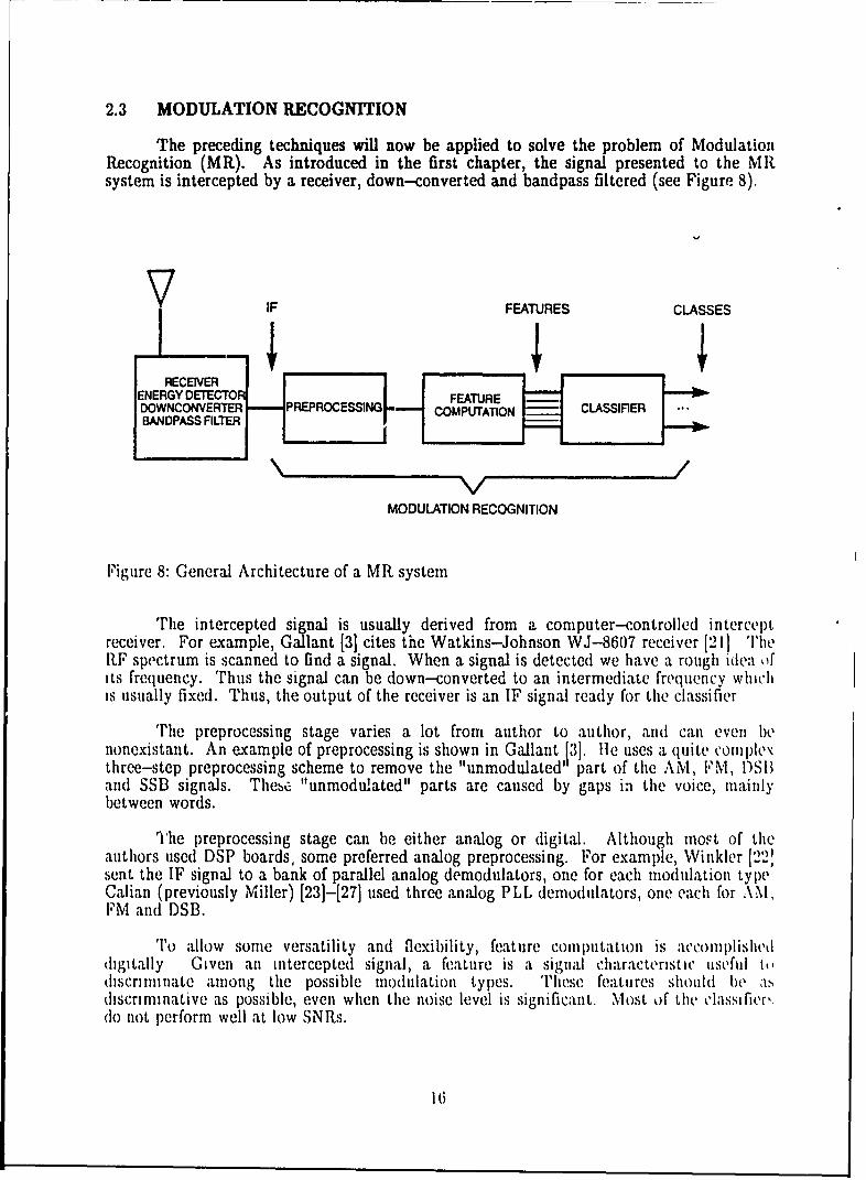
The preceding techniques will now be applied to solve the problem of ModulationRecognition (MR). As introduced in the first chapter, the signal presented to the MRsystem is intercepted by a receiver, down-converted and bandpass filtered (see Figure 8).

y IF FEATURES CLASSES

RECEIVERENERGY DETECTOR FEATUREDOWNCONVERTER PREPROCESSING COMPUTATION CLASSIFIERBANDPASS FILTER

MODULATION RECOGNITION

Figure 8: General Architecture of a MR system

The intercepted signal is usually derived from a computer-controlled interceptreceiver. For example, Gallant [3] cites the Watkins-Johnson WJ-8607 receiver [21] Tl'heRF spectrum is scanned to find a signal. When a signal is detected we have a rough idea ofits frequency. Thus the signal can be down-converted to an intermediate frequency whIchis usually fixed. Thus, the output of the receiver is an IF signal ready for the classifier

The preprocessing stage varies a lot from author to author, and can even benonexistant. An example of preprocessing is shown in Gallant [3]. lie uses a quite complexthree-step preprocessing scheme to remove the "unmodulated' part of the AM, FIM, DSI3and SSB signals. Theb,3 "unmodulated" parts are caused by gaps in the voice, nainlybetween words.

tr1he preprocessing stage can be either analog or digital. Although most of theauthors used DSP boards, some preferred analog preprocessing. For example, Winkler [221sent the IF signal to a bank of parallel analog demodulators, one for each modulation typeCalian (previously Miller) (231-[271 used three analog PLL demodulators, one each for AM,FM and DSB.

To allow some versatility and flexibility, feature computation is accomjplisheddigitally Given an intercepted signal, a feature is a signal characteristic useful todiscrillnate among the possible modulation types. These features should be asdiscriminative as possible, even when the noise level is significant. Most of the classifivr ,

do not perform well at low SNRs.

16

The decision procedures considered by the authors are represented by the twotechniques explained in Section 2.2: the linear and the decision tree classifiers. Thedecision tree technique considered here consists of the simplest form: questions of the type"Is z4 > 3.2?", where 3.2 would have been obt2ined during the training phase. Moreoverthe tree is not optimized: instead of using a sophisticated algorithm like CART toestablish the optimal splits and thresholds, the sets of rules are defined empirically bylooking at the training data. Note finally that th? tree is sometimes presented inalternative ways: boolean equations or logic table (see Figure 9).

xl

A \ A = (xl>Th1)(x2>Th2)

BB = (x2<Th2)C - C = (xl<h1)(x2>Th2)

a) Decision Region b) Boolean Equations

B A

xl x2 B 0 1

A >Th1? 1 >Th2? 1

B >Thl? X >Th2? 0 C 11>Th1

C >Thl? 0 >Th2? 1- x2>h2

c) Logic Table d) Binary Tree

Figure 9: Illustration of the logic tree decision process.

Usually the authors especially the latest ones, will use a linear classifier. Howeverone author, Jondral [28][29f, got slightly better results with a quadratic classifier.

To collect the information on MR, a literature search has been conducted. All thepapers reported here are unclassified. They report an interest in recognizing both analogand digital modulations: AM, SSB, DSB, FM, ASK,OOK, BPSK, QPSK and FSK. Froma military perspective, Torrieri [30] in his book says that the importance of analogcommunication systems is declining, probably due to the proliferation of digital computersand the security provided by cryptographic digital communication. Thus in the last yearbmore papers have been published on digital modulation classifiers. Nevertheless, analo'tgcommunications are still in use and the problem of analog modulation classification tillretains some interest.

17

The techniques for modulation classification described in the following pages havebeen grouped depending on whether the author put more emphasis on analog or digitalmoduJation schemes. Within each group, the authors have been gathered according tosome s'milarities, as shown in Table 1. In the table, 'I?" refers to a modulation type forwhich it was not clear whether or not the MR algorithm was able to recognize.

18

MODULATION TYPESEC-

GROUP AUTHOR TION ANALOG DIGITAL

A S D F A F B QM S S M S S P P OTHER

B B K K S SK K

Miller 3.1 / / / / /Luiz / / / / /Wakeman / V / / /Fry V / / /

Gadbois 3.2 / / / / /Ribble / / / / / / /UTL / / / / / /Gallant / / / /

ANALOG Weaver 3.3 / / /Winkler / / / /Callaghan / / / ? ?Fabrizi / / /Petrovic / _ / / /

Aisbett 3.4 / / /Einicke / / ? /

Hipp 3.5 777V7777 _

Liedtke 4.1 / / / / 4-FSK8-PSK

Jondral I / / / / 4-FSKDominguez V / / / / / / / 4-ASK

DIGITAL 4-FSKAdams

Mammone 4.2 / /DeSimio / / / /

Ready 5.1 ? ? ?ENERGY IDETEC- Kim 5.2 /

TOR Gardner 5.3

Table 1: Groups of authors.

19

3.0 MR FOR ANALOG MODULATIONS

This group is bigger for a historical reason: the first paper was written in 1969.The interest in digital modulation is more recent. The particularity of this group is thefeatures used. Because analog modulations are dominated by amplitude modulation (AM,DSB, SSB), the signal envelope is a characteristic somewhat exploited by several authors,starting with Gadbois in 1985. Before that, authors were using a hardware approach as wewill see with Miller.

3.1 MILLER APPROACH

3.1.1 Miller

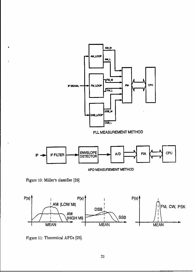
In 1978, Miller Communications Systems Limited (now Calian CommunicationsSystems Limited) presented a report [23] to DREO on the feasibility of a HF/VHFspectrum surveillance receiver, including automatic modulation type identification. DREOliked the idea and prepared a contract for a prototype ESM receiver. The approachdeveloped by Miller for modulation classification prevailed for years and led to a number ofpublications [23]-[27][31][321[7].

In their implementation, the receiver produces a 455kHz IF signal (with a passbandfilter of baudwidth either 6 or 24 kHz) which is fed to an envelope sampler APD(Amplitude Probability Distribution) and three parallel phase-lock-loop (PLL)demodulator circuits (see Figure 10).

The method used to characterize the signal amplitude envelope is called APD(Amplitude Probability Distribution). As shown in Figure 10, the output of the envelopedetector is sampled by an 8 bit ADC (with a sampling rate of 1.7kHz). N points were usedto compute the following statistics:

Mean:/J = 1 E (x)

Variance: S2 = [ (x2) - 1 ()J

P (x): Probability that the ADC output is equal to x,corresponding to the APD (see Figure 11).

After an inspection of 213 samples, Miller found that good statistical significance wasobtained and could be useful for modulation classification. However, to keep the number -ffeatures low, only two APD parameters have been retained: the variance S2 and theprobability that the output of the ADC equals 0, P (0).

2(0

AM LOOP

AM-L

FSIGNA-. M.O SSBM PIA CPU

DB-

PLL MEASUREMENT METHOD

IF IF ILTERDETECTOR

APD MEASUREMENT METHOD

Figure 10: Miller's classifier [25]

P(x) P(x) P(x)AM (LOW il

AMB A FM, CW, PSK

HIGH MI) SB

MEAN MEAN MEAN

Figure 11: Theoretical APDs [251.

21

In a similar way, Miller studied the output of the PLL circuits in order to use theproperty that different types of PLL circuits have a tendency to lock onto different signals.Each of the three loops (AM, FM and DSB) has 2 outputs used for the classification: aLock indicator and a Modulation indicato:. Considering 4096 samples, Miller created atable which is reproduced in Table 2. This table shows which PLL is locked to whichmodulation type.

Combining both APD and PLL results, Miller created a Reference Logic Table (seeTable 2). The table contains eight binary features: two from the APD and six from thePLL. The binary values are the results of hard decisions on the outputs of the ADCs withreference thresholds.

SIGNAL AM-M AM-L FM-M FM-L IDSB-M DSB-L S2 P (0)

AM 1 1 0 1 1 1 1 0

FM X 0 1 1 X 0 0 0

PSK 1 0 1 1 1 1 0 0

CW 0 1 0 1 0 1 0 0

DSB X 0 1 0 1 1 1 1

SSB X 0 X 1 X 0 1 1

Threshold .312 .812 .625 .500 .250 .812 256 .004

Table 2: Miller's Reference Logic Table [25].

The classification is accomplished by comparing the unknown with the referenretable for a perfect fit. To use the terminology introduced in Section 2, it is a very simplebinary tree classifier. 'he bandwidth of the passband filter is first set at 24 kHz. If thereis no match for the classification, another attempt is made with the 6 kHz filter.

The results obtained by Miller are quite impressive. They claim a percentage ofcorrect identification higher than 90% for all modulation types. However, the SNR is notspecified. To get these results, the classifier used 256 samples per try and a minimum offour tries per classification.

As stated previously, the Miller prototype ESM receiver was built under a DNDcontract. An evaluation of Miller's work is reported by Luiz in [31].

22

3.1.2 Wakeman

In 1985, a U.S. Patent was registered [32] for a "Spectrum Surveillance ReceiverSystem". It is Miller's receiver, no upgrade to the classification procedure has beenreported.

3.1.3 Fry

Fry [7] also looked at iller's receiver. Some problems had been reported', and Frywas assigned by DREO to determine their origins. After some tests, he found that due tothe nature of the PLL design used, the accuracy of the identification process deterioratedrapidly if the receiver was not tuned to the c, tex of the signal. He also noted thatidentification failed with real voice signals. Tests with the modified prototype(modification both in the hardware and decision tree) revealed 95% correct identificationwith a 10dB SNR, when a sine wave was used as modulating signal. Unfortunately, theaccuracy fell drastically for real voice signal. With an infinite SNR (no noise) and a realvoice signal (normal gaps associated with continuous speech), he got an averageperformance around 60%.

3.2 GADBOIS APPROACH

3.2.1 Gadbois

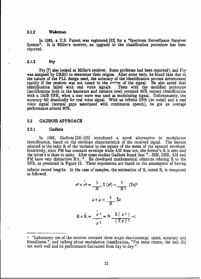
In 1985, Gadbois [33]-[35] introduced a novel alternative to modulationidentification, based on the envelope characteristics of the received signal. The featureselected is the ratio R of the variance to the square of the mean of the squared envelope.Intuitively, since FM has constant envelope while AM does not, the former's R is zero andthe latter's is close to unity. After some studies Gadbois found that "...SSB, DSB, AM andFM have very distinctive R's...". He developed mathematical relations relating R to theSNR, as presented in Figure 12. These expressions are based on the assumption of having

infinite record lengths. In the case of samples, the estimation of R, noted R, is computedas followed.

0.2 - a-2 1 E (z2)_ 1 () 2

N N2

1N

RzR= r 2 =N E(z 2 ) -

1 "Laboratory use of the receiver revealed three major shortcomings. speed, accuracy andfriendliness.", and talking about modulation classification, "For some reason, the unit didnot work well and its performance fluctuated from day to day.".

23

2.0 DSB

0'1.0 SSB

1 .0 A M0.5 E FM

0 10 15 20CNR (dB)

Figure 12: Mathematical relations relating R to the SNR [35, p.1521.

Computing R for N=2048 points per sample for a large number of samples, Gadboisdetermined threshold values within a small decision tree for classification of AM, SSB,DSB and FM. In his experiments, the voice was simulated by Gaussian white noiselow-pass filtered. The sampling rate for the 12-bit ADC was 160kHz. The IF frequencywas 40kHz. The results of that very simple classifier were computed from 200 samples permodulation type and are presented here in Table 3.

ACTUAL CLASSIFIED AS

FM AM SSB DSB

FM 200 0 0 0

AM 0 181 19 0

SSB 0 15 160 25

DSB 0 0 12 188

Table 3: Gadbois' confusion table [33, p.29.5.41.

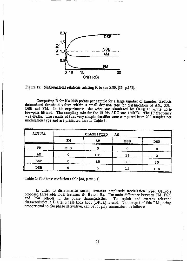
In order to discriminate among constant amplitude modulation type, Gadboisproposed three additional features: R2, R3 and R4. The main differcnce between FM, FSKand PSK resides in the phase characteristics. To exploit and extract relevantcharacteristics, a Digital Phase Lock Loop (DPLL) is used. The output of this PLL, beingproportional to the phase derivative, can be roughly summarized as follows:

24

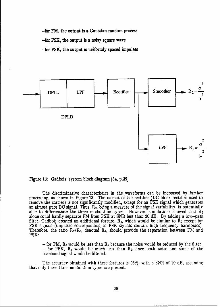
-for FM, the output is a Gaussian random process

-for FSK, the output is a noisy square wave

-for PSK, the output is uniformly spaced impulses

2

DPLL LPF Rectifier Smoother R2 =-2

DPLD

2

LI LPF -- 0 R3= G

Figure 13: Gadbois' system block diagram [34, p.39]

The discriminative characteristics in the waveforms can be increased by furtherprocessing, as shown in Figure 13. The output of the rectifier (DC block rectifier used toremove the carrier) is not significantly modified, except for an FSK signal which generatesan almost pure DC signal. Thus, R2, being a measure of the signal variability, is potentiallyable to differentiate the three modulation types. However, simulations showed that R2alone could hardly separate FM from PSK at SNR less than 20 dB. By adding a low-passfilter, Gadbois created an additional feature, R3, which would be similar to R2 except forPSK signals (impulses corresponding to PSK signals contain high frequency harmonics)Therefore, the ratio R2/R 3, denoted R4, should provide the separation between FM andPSK:

- for FM, R3 would be less than R2 because the noise would be reduced by the filter- for PSK, R3 would be much less than R2 since both noise and some of thebaseband signal would be filtered.

The accuracy obtained with these features is 98%, with a SNR of 10 dB, assumingthat only these three modulation types are present.

25

3.2.2 Ribble

Using methods similar to Gadbois, Ribble [91 developed his system around the samefeatures R, and R2 , but replaced R3 and R4 by ACPOW (see Figure 14).

SHIL.BERT 0

TRANSFORMER R1 -

BANDWIDTHESTIMATOR BW

IFINPUT"-

LOCKED LOOP REMOVER - =

ACOUT

ACPOW = ACOUTr ACIN

ACIN)

Figure 14: Ribble's system block diagram [9, p.20].

In the block diagram, R, is Gadbois' ratio R, and R2 is almost like Gadbois'. Thelast feature is a power parameter, ACPOW. It measures the power at the DPLL output'.Thus it gives the value of the amount of phase/frequency changes in the signal. For digitalmodulation schemes, the value of ACPOW decreases with the baud rate.

Once again the decision process uses a logic tree. The value of R is used only toseparate Group B (phase modulations) from Group A (amplitude modulations) The otherfeatures will complete the estimation of the modulation type. The time required for the

It is given that ACPOW = ACOUT/ACIN. Here ACIN is a normalisation factor.

26

computation and the decision is 1.7sec. The performance obtained is about the same asGadbois', but Ribble reduced the sampling time. He pushed the experiments further andreplaced the simulated voice by real voice, obtaining drastically lower accuracies. HoweverRibble did not go further with the problem and concluded his report with this comment:

"If the prime modulating signal of concern is voice then a different data acquisitionprocess will be necessary. It would have to reject segments of low/no modulationand stack together those segments which indicate modulation is present. Thiswould obviously result in extremely long time frames to analyze voice, but thisseems to be the only way to cope with this situation." Ribble [9, p.721.

3.2.3 UTL

In 1989, DND/DEEM 4 gave a contract to UTL CANADA INC. [36] for ananalytical examination of various classification techniques (Jondral, Callaghan, Gadbois,Ribble, Fabrizi, Wakeman and Gardner). The contract aso asked for the design of aprototype MRU (Modulation Recognition Unit).

UTL decided that Ribble's approach was the most promising and tried to improvethe performance further. The block diagram was roughly the same. However thealgorithm for evaluation of the bandwidth was "improved". The logic tree for the decisionprocess was also changed, incorporating a new feature, the product of the precedingfeatures R, and R2. The hardware was set with the following conditions: IF frequency of34kHz with 12kHz bandwidth and a sampling frequency of 140kHz. The performance wasnot significantly improved and the results or real voice were still unsatisfying (averageprobability of success around 25%).

3.2.4 Gallant

Neither Ribble nor UTL were able to obtain good performance with Gadbois' ratio.Gallant [3] looked at the problem again and got very interesting results.

First of all he considered the problem of real voice signals. The preceding authorsgot good results with simulated voice, but their performance fell drastically with real voice.They all agreed that the gaps in voice signals create "unmodulated" segments which areimproper to classify the signal.

"1. Unmodulated AM and FM produce a pure carrier signal; hence they areindistinguishable from each other and CW; and

2. Unmodulated SSB and DSB produce no transmitted signal; hence they areindistinguishable from each other and noise" Gallant [3, p.24]

In order to solve this problem, Gallant added a preprocessor to Gadbois' algorithm.before computing the ratio R, the preprocessor removes the unmodulated segments. Thispreprocessor is comprised of three steps which will now be described.

27

The first two steps permit the MIlD to reject long stretches of unmodulatedwaveform on a segment to segment basis'. This procedure is performed by the Front-Endwhich is divided in two parts: the first part rejects low-energy segments, the secondrejects noise-like segments.

Looking at the behavior of R. Gallant found that "anomalies" occur when themodulated signal envelope is small. The third step consists of rejecting low-valuedenvelope sampling points, on a point to point basis. When N good points are collected, a"pseudo fully-modulated" segment of 2048 points is formed.

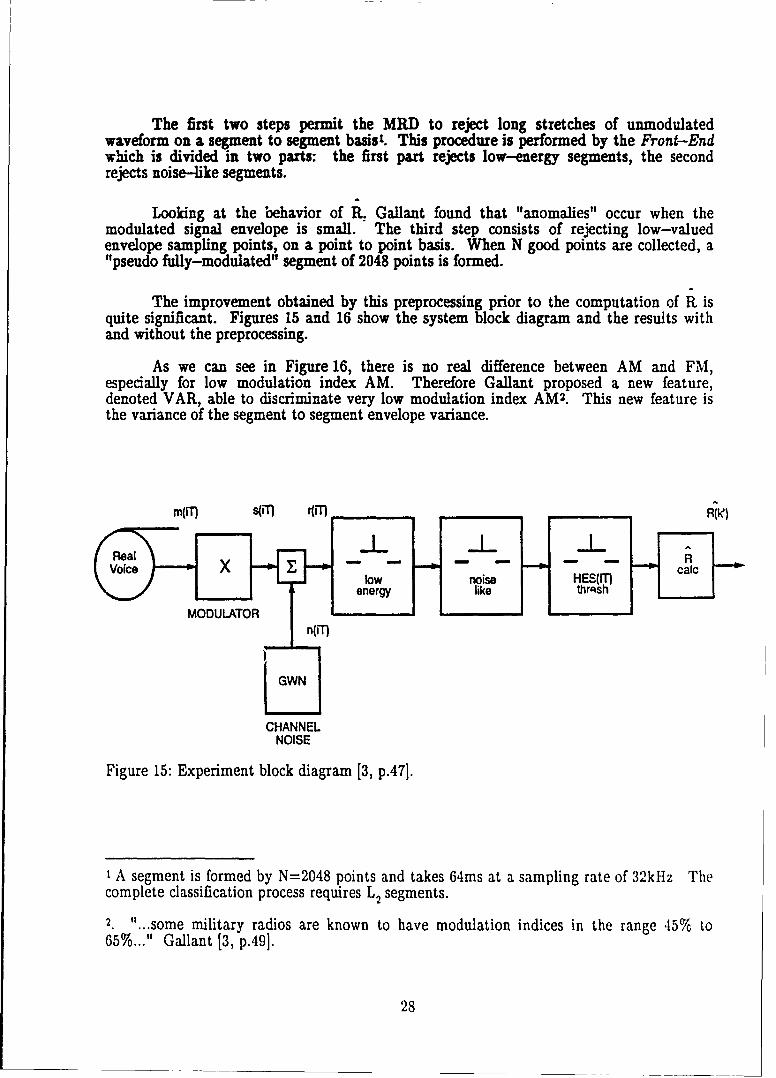
The improvement obtained by this preprocessing prior to the computation of R isquite significant. Figures 15 and 16 show the system block diagram and the results withand without the preprocessing.

As we can see in Figure 16, there is no real difference between AM and FM,especially for low modulation index AM. Therefore Gallant proposed a new feature,denoted VAR, able to discriminate very low modulation index AM2. This new feature isthe variance of the segment to segment envelope variance.

m( s(71 r(iT RWke)

RealRlow noise HES(rT) caic

energy like thr'sh

MODULATORn(iT

GWN

CHANNELNOISE

Figure 15: Experiment block diagram [3, p.47].

I A segment is formed by N=2048 points and takes 64ms at a sampling rate of 32kHz Thecomplete classification process requires L2 segments.

2. "...some military radios are known to have modulation indices in the range .45% to65%..." Gallant [3, p.49].

28

GADBOIS ALGORITHM

0 8

w 6 -50--- DSB

(0- SSBz

AMo IFM

0 10 20 30 40 50 60 70 80 90 100C/N (dB)

NEWALGORITHM

2.8

02.42.0

~1.6 DSB0

<T T AM

0 FM

o 10 20 30 40 50 60 70 80 90 100

C/N (0B)

Figure 16: Variance of R diminished by preprocessing.

a) Gadbois' ratio R (Gallants experimental results) [3, p.231b) New feature proposed by Gallant [3, p.48]

29

The new feature VAR is computed as followed:

L2

MEAN = E{o2 (k)} = 0,2 (k)L 2 k u!

t2

VARJo2 (k)} = [o,2 (k) - MEAN2L 2 kzl

L2: The number of segments whichpassed the front-end section.

NEW ALGORITHM

40 I

30AM (100% .ll)

20-10 ,AM (50% MI)

coLa AM (10% Mi)n-_ 0 . ...

-10

-20-

NBM WBFM-30

0 10 20 30 40 50 60 70 80 90 100C/N (dB)

Figure 17: The new feature VAR proposed by Gallant [3, p.54].

30

The decision process is also a logic tree, however much simpler than Ribble'sbecause there are only two features. The performance obtained with real voice and SNRsabove 8dB is quite good (90%). However the acquisition time is long : at least 1.5 seconds.

3.3 OTHERS

3.3.1 Weaver

Probably the first author to publish about modulation type classification isWeaver [37] in 1969. He proposed the use of pattern-recognition techniques toautomatically identify the type of modulation on HF radio signals. The intercepted signalwas passed through an 8kHz analog bandpass filter and down-converted to baseband. Itwas then digitized with an 8-bit ADC at a 16kHz sampling rate. The resulting digitalsignal fed a bank of 29 parallel narrowband filters and envelope detectors. The outputswere averaged over an observation time of one second. These mean values created a29-dimension feature vector used for the decision process. The classifier is an analogimplementation of a linear classifier. Weaver claims 95% classification accuracy at"typical" SNRs for separating AM and SSB. He warns that speech breaks give rise tounmodulated signals and a real system may require several seconds of observation time.

3.3.2 Winkler

Winkler [221, proposed a technique based on characterizing the amplitude andphase spectrum. He used a pure sinusoid as the modulating signal. He obtained 100%accuracy, although he admitted that gross classification errors occur when the basebandsignal has a noisy spectrum.

3.3.3 Callaghan

Callaghan [38] also based his classifier on the classical pattern-recognition theory,he used a linear classifier. He sampled the signal envelope and amplitude zero-crossing (toget the instantaneous frequency). Then he computed the means and the standarddeviations. The sampling frequency was 100Hz and the observation time, 2 seconds. Hereported only the performance for separating AM to FM: 99% for an SNR above 20dB.Callaghan concluded his paper admitting that his features were very sensitive to noise.

3.3.4 Fabrizi

Instead of considering the variability of the envelope, Fabrizi [39] suggested a newfeature, the envelope peak to mean ratio noted P,. He also used the mean M of theinstantaneous frequency.

The information comes from Gallant[gallant, p.9-10], the reference is not available at this

time.

31

SSB 400" = 0SSB

thresholdth Af = 1.6kHzthresholdthreshold th

Pe = M (dB)

2 AMm 0.6

threshold th21 - e _ - - =10- C

CW/FM Af = 1.6kHz

0I I I I _0

0 10 20 30 40 50 60 70 80 0 10 20 30 40 50 60 70 80S/N (dB) S/N (dB)

Figure 18: Fabrizi's features [39, p.138].

With only these two features Fabrizi built a logic tree for the decision process(see Figure 19). The parameters were collected over a 250ms sampling time, using 32kasampling frequency and 3kHz filtered real voice. Simulations showed that separation ofAM from FM using the instantaneous frequency parameter could not be achieved at SNRsbelow 35dB. However, SSB could be separated from AM/FM group at SNR above 5dB.

Figure 19: Fabrizi's Decision Tree [39, p.139].

32

3.3.5 Petroic

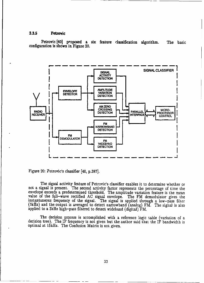
Petrovic [40] proposed a six feature classification algorithm. The basicconfiguration is shown in Figure 20.

SIGNAL SIGNAL CLASSIERACTIVITY --,II

ENVELOPE AMPLITUDE~DETECTIONyI d

-- AMZEROCROSSING MICRO-

RADIO DETECTION PARALLE PROCESSORRECEIVER INTERFACE CONTROL

F IM" "DETECTION

~FMD - EMODULATOR F

- • WIDEBANDDETErCTIONI Il

Figure 20: Petrovic's classifier [40, p.387].

The signal activity feature of Petrovic's classifier enables it to determine whether ornot a signal is present. The second activity factor represents the percentage of time theenvelope exceeds a predetermined threshold. The amplitude variation feature is the meanvalue of the full-wave rectified AC signal envelope. The FM demodulator gives theinstantaneous frequency of the signal. The signal is applied through a low-pass filter(3kHz) and the output is averaged to detect narrowband (-analog) FM. The signal is alsoapplied to a 3kHz high-pass filtered to detect wideband (digital) FM.

The decision process is accomplished with a reference logic table (variation of adecision tree). The IF frequency is not given but the author said that the IF bandwidth isoptimal at 15kHz. The Confusion Matrix is not given.

33

3.4 AISBETT APPROACH

A lot of work has been done at the Electronic Research Laboratory, Department ofDefence, Defence Research Centre Salisbury, Adelaide, South Australia regardingmodulation recognition. New features , which are claimed to be "noise resistant" arepresented by two authors, Aisbett and Einicke in this section.

3.4.1 Aisbett

Almost every paper presented proposed features which are very sensitive to noise.For example, remember that Fabrizi was not able to separate AM from FM at SNRs below35 dB. Aisbett [41][42] closely considered the problem of additive white Gaussian noise(AWGN) regarding time-invariant features for pattern recognition.

She observed that most published modulation recognition schemes perform poorlybecause the authors chose signal parameters which can only be estimated with a bias in thepresence of AWGN. She shows, for example, how the sample mean and sample variance ofthe instantaneous frequency varies with SNR for a number of analog modulation typesThus she proposed time-domain signal parameters which are unbiased estimators of thetrue signal parameters in the presence of AWGN with symmetric spectral density.

The three new proposed noise resistant features are A2, AA' and A20', where A isthe signal envelope, A' the signal envelope derivative and 0' the instantaneous frequencyConsidering very low SNRs (3dB), she claims discrimination between AM, FM DSB andCW possible on the basis of characterizing the new parameters' statistical distributionfunctions.

896 917

DSB

~ZAM

noiseZ

FM(narrowband) M-:Z FM(wideband)

Q I I Th%.%.. IAM DSB8d

A -3.7 -8dB A20, 8dB

Figure 21: Distributions of Aisbett's parameter A2 0'and the typical parameter A (SNR = 1dB) [41, p.12, 171,

34

It is shown in Figure 21 that for very low SNR (-1 to 3dB), the typical parameter A(signal envelope) has a distribution function which offers no discrimination between themodulation types. However the distribution functions for Aisbett's parameter A20' aredistinct and could therefore be used for classification.

She was satisfied by her preliminary work and envisaged further simulations with amuch larger data base in order to implement a classifier using a pattern-recognitionalgorithm applied to these new features.

3.4.2 Einicke

A few years later, a paper written by Einicke [6] was published. He described aclassifier based on Aisbett's features.

A2 =2 + Q2AA'= II' + QQ'A201 = IQ? - IQ

He added two classical parameters, the signal envelope and instantaneous frequency

A )A1/2

F = 0' = (A20')/A2

As stated by Aisbett, the statistical distribution of these parameters should have agood discriminating power even for low SNRs. Jondral's method' of using the histogramas a features vector is potentially very powerful. However the computation required is tooexhaustive for a real time system. One of the best ways to describe a statisticaldistribution is to use the standard deviation a, the coefficient of skewness 'y and thekurtosis /0.

The feature vectors are computed for each modulation type according to threeclasses of signals: strong signal (30dB), medium (15dB) and weak (5dB). The parametersin the data base are obtained through digital signal processing of data generated from12-bit ADC having a sampling rate of 20 kHz. For the decision process, a linear classifier(Fisher's functions) is applied to these reference feature vectors. He also tried a quadraticclassifier but found no improvement. The performance obtained depends on the sampleacquisition time. For an acquisition time of 409ms, the overall performance is around 94%(5dB < SNR < 30dB).

See the digital modulation section.

35

3.5 HIPP APPROACH

3.5.1 Hipp

This area of modulation classification is very intuitive. The choice of the featuresdepends upon the author's background, imagination, etc. Hipp [8] used a different way toselect his features. He did a systematic and exhaustive evaluation of more than twentyfeatures from which he retained only six. The results obtained are very impressive: heclassified almost all modulation types (digital and analog) with an overall performance of95% with SNRs going down to 10dB. His paper is presented in a distinct section for thesereasons.

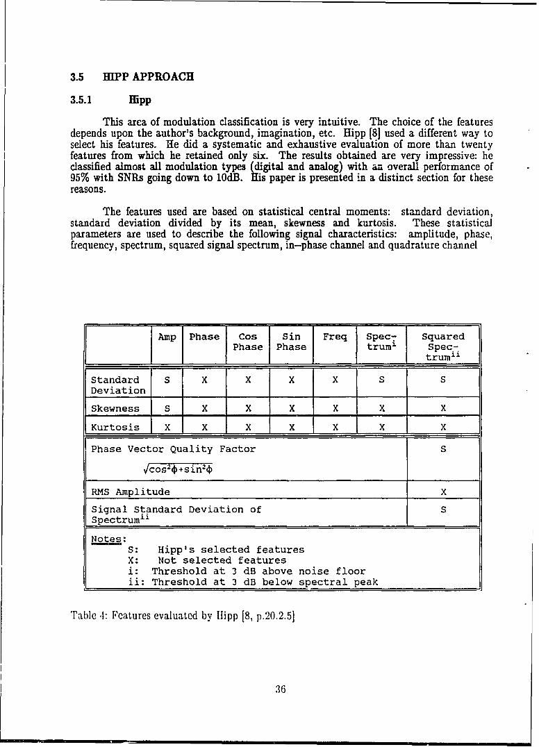
The features used are based on statistical central moments: standard deviation,standard deviation divided by its mean, skewness and kurtosis. These statisticalparameters are used to describe the following signal characteristics: amplitude, phase,frequency, spectrum, squared signal spectrum, in-phase channel and quadrature channel

Amp Phase Cos Sin Freq Spec- SquaredPhase Phase trum- Spec-

trum"

Standard S X X X X S SDeviation

Skewness S X X X X X X

Kurtosis X X X X X X X

Phase Vector Quality Factor S

vcos 24+Sinf2

RMS Amplitude X

Signal Standard Deviation of SSpectrumii

Notes:S: Hipp's selected featuresX: Not selected featuresi: Threshold at 3 dB above noise floorii: Threshold at 3 dB below spectral peak

Table 4: Features evaluated by Ilipp [8, p.20. 2.51

36

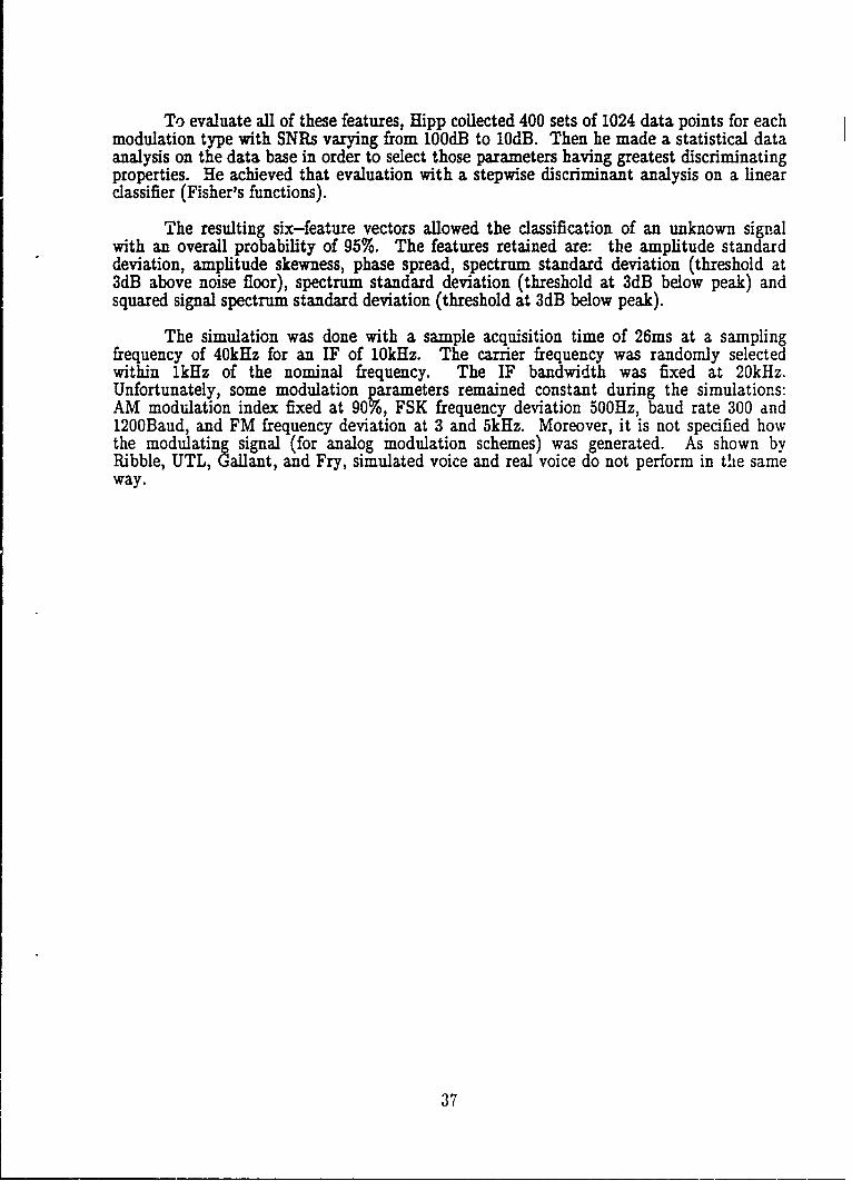
To evaluate all of these features, Hipp collected 400 sets of 1024 data points for eachmodulation type with SNRs varying from 100dB to 10dB. Then he made a statistical dataanalysis on the data base in order to select those parameters having greatest discriminatingproperties. He achieved that evaluation with a stepwise discriminant analysis on a linearclassifier (Fisher's functions).

The resulting six-feature vectors allowed the classification of an unknown signalwith an overall probability of 95%. The features retained are: the amplitude standarddeviation, amplitude skewness, phase spread, spectrum standard deviation (threshold at3dB above noise floor), spectrum standard deviation (threshold at 3dB below peak) andsquared signal spectrum standard deviation (threshold at 3dB below peak).

The simulation was done with a sample acquisition time of 26ms at a samplingfrequency of 40kHz for an IF of 10kHz. The carrier frequency was randomly selectedwithin 1kHz of the nominal frequency. The IF bandwidth was fixed at 20kHz.Unfortunately, some modulation parameters remained constant during the simulations:AM modulation index fixed at 90%, FSK frequency deviation 500Hz, baud rate 300 and1200Baud, and FM frequency deviation at 3 and 5kHz. Moreover, it is not specified howthe modulating signal (for analog modulation schemes) was generated. As shown byRibble, UTL, Gallant, and Fry, simulated voice and real voice do not perform in the sameway.

37

4.0 MR FOR DIGITAL MODULATIONS

The interest in digital modulation classification is growing yet the number ofpublications is still small. For this reason all the classifiers are represented by only twogroups. The first one is represented by Liedtke and Jondral. These two authors, especiallythe latter, are very well known and are cited in almost every paper on the topic. Thesecond group includes authors who used a different approach to Liedtke's.

4.1 LIEDTKE AND JONDRAL APPROACH

4.1.1 Liedtke

One of the first authors to publish about modulation type identification, Liedtke [2]was also the first to present the concept of modulation recognition applied to digitalmodulation schemes. The system proposed by the author is fully digital, as shown inFigure 22. The output of the receiver is digitized (In-phase and Quadrature channels) andthen filtered by a bank of parallel FIR narrow-band filters. These filters have the samecenter frequency but different bandwidths. "The best classification result will beautomatically obtained behind that filter which matches the signal bandwidth best."

The feature extraction is accomplished with a "universal demodulator". Thesefeatures are the amplitude, phase and instantaneous frequency (see Figure 23). To get theparameter values in a synchronous way, a timing recovery procedure is used. Theparameters are defined as:

Amplitude = (12 + Q 2)112

Instantaneous Frequency 1 [dso( t)]2 L dt t=ti

1 o, - 'Pi-

2 r 2 At

V arctan (Q/I)

The values are compiled to form histograms of amplitude, frequency and phase.These histograms are used as features for the classification. The 256-point phasehistogram of BPSK has peaks at 0 and 1800. Foi QPSK, the peaks are located at 0, 90,180 and 270". And likewise for 8-PSK. Therefore the phase histogram is used to classifythese modulation types. The object is to use the histogram as input to a procedure thatwill recognize the number of ph;.ses. A pattern-recognition algorithm could be used,taking each cell of the histogram as an element of the feature vector. However, to simplifythe computation, Liedtke used suboptimal weighting functions, as shown in Figure 24

38

*000

Univrsaldemn~uorI

Clrcultsforaccumulackn Avtsin CUMforthe hisoram the varitd a sba ances of

Microcomputer for featureanalysis and classifIcabon

Figure 22: Block diagram of Liedtke's classifier [2, p.313].

FigureR 23: Lid2e' unvra dem duatrcto.r

39mu

*5. S: :*: .: ::N--240"

NUMBER •OF :

EVENTS : . ..* S 5.5..... .a. • :O . .. .* S-.."555 55" 5 .. . 5.. . . -S . ...

I I '-180 -90 0 90 180

Ap (Degree)

a)

WL 0 I I I

-90 0 eo 180-1 e. .0046 90

b)

Figure 24: Classification of PSK signals by Liedtkeal Actual phase histogram for QPSK [2, p.315]b)Suboptimal weighting function for QPSK [2, p.3 16]

The unknown signal phase histogram is compared to the weighting functions and avalue of similarity is attributed to each. The largest output is retained and noted DPHI,corresponding to the number of phases detected (2, 4 or 8).

If the recognition criterion of PSK modulation types is not satisfied, theclassification of ASK and FSK is investigated. To identify these modulations, thevariances of the amplitude and frequency (AVAR and FVAR respectively) are calculated.A large AVAR indicates ASK, and a large FVAR, FSK.

In a similar way to the phase histogram, the amplitude and frequency histogramsare also used. The amplitude histogram of ASK contains two peaks, as does the frequencylustogram for FSK. These histograms should contain only one peak for other modulationschemes. The resulting variables are respectively AHI and FHI.

40

The decision process is accomplished with three boolean equations: one for the PSK

modulation type, one for ASK and one for FSK. The decision function for PSK is

[(max (DPHI))i>2 > TDPHI]-[AVAR < TLAVAR]-[FVAR < TFVAR = TRUE

i=2,4 or 8 is the number of phasesTDPHI is the threshold for the phase histogram

TLAVAR is the threshold for the amplitude varianceTFVAR is the threshold for the frequency variance

the symbol - is a logical AND

If the function is "true" for i=2, BPSK is detected; if i=4, QPSK is detected; and ifi=8, 8-PSK is present. Otherwise, i.e. DPHI is optimal for i=1, the test continues forASK and FSK. The equations are the followings.

[AHI > TAHII- [AVAR > TUAVAR] = TRUE.. for ASK and[FHI > TFHI -[FVAI> TFVAR]-[AVAR < TLAVAR] = TRUE...for FSK

TAHI is the threshold for AHITUAVAR is the upper threshold of amplitude variance

TFHI is the threshold for FHI

These functions and the thresholds are schematized in Figure 25. The fiveseparation parameters are shown together. The dashed lines point out which classes areseparated by which separation parameters. The overlapping between PSK and FSKindicates some remaining difficulties.

Noise andFSK FHI continuously AHI ASK

2 modulated 2

FVAR 2 4AFVAR (PSK 4.PSK 8) 2<

Figure 25: Schematized class space with separation parameters [2, p.3181.

,41

The results shown in Figure 26 indicate a classifier very sensitive to noise.

Pe 10- 10 -410 Pe 102 10"310"4100 100PSK 2 ASK 2

a. I

0 0L

0 5 10 10 15ET/no (dB) Er/no (dB)

10-2 10-3 10-4 10-2 10-310 -4

10 10200~o-

t PsK 4 FsK 2,

M II I

5 10 15 5 10

Er/no (dB) ~ E/n o (dB)

Figure 26: Liedtke's results [2, p.3191.

4.1.2 Jondral

Jondral [28][29 ] used an approach similar to Liedtke's to which he added two analogmodulation types (AM and SSB) and pattern-recognition techniques for the decisionprocess.

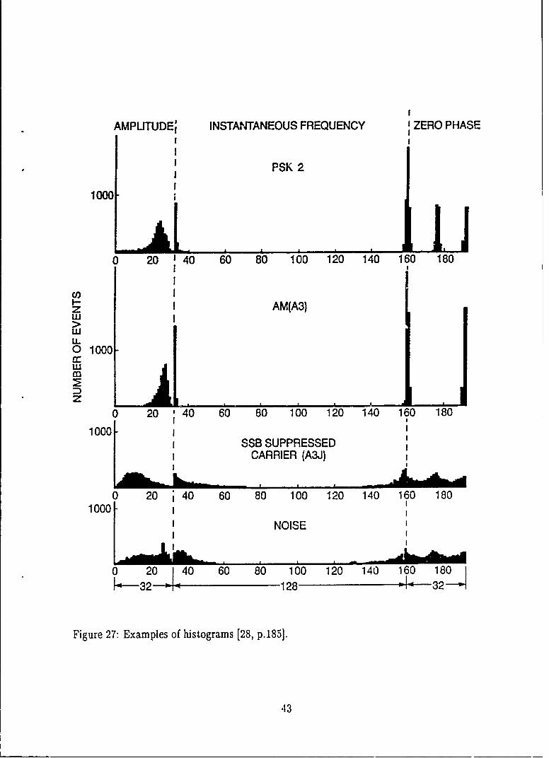
The features used by the author are bared on histograms. However, he did not useLiedtke's synchronization system. Therefore the histograms are different, although theparameters are similar: amplitude, instai caneous frequency and pliase. The phasecharacteristic called zero phase, used to det'ct BPSK, is obtained by squaring the signal tocreate a carrier at twice the frequency which can be caught by a tracking loop, resulting inthe detection of 0 and 7r phases in BPSK signal.

Collecting the parameters for 4096 points, a histogram of 192 cells is computed (seeFigure 27). This histogram is used as the feature vector. However, Jondral realized thatthe features between positions 60 and 140 do not contribute to the discrimination. Thefinal results were obtained with 93-D feature vectors. This is remarkably bigger thanGadbois, who used only a few features.

42

AMPUTUDE; INSTANTANEOUS FREQUENCY ZERO PHASE

PSK 2

II1000

0 20 40 60 80 100 120 140 160 180

I AM(A3)wLL0 1000-tLw

Dz ~0 20 '40 60 80 100 120 140 160 180

I Io1000-

1001.SSB SUPPRESSEDCARRIER (A3J)

~A0 20 40 60 80 100 120 140 160 180

1000!

INOISE

0 20 140 60 80 100 120 140 160 180

[--214128 01L -3

Figure 27: Examples of histograms [28, p.185].

,43

The performance obtained is very good, but the SNRs are not specified. The systemoperated for a signal down-converted at 200kHz. The 12-bit ADC sampling frequency ischosen according to the IF signal bandwidth: 2.2kHz to 22.2kHz respectively for 300Hz to6kHz. To acquire the 4096 data points, an acquisition time of 0.18 to 1.8 seconds wasrequired. The decision function was based on a pattern-recognition technique. Jondraltried both linear and quadratic clas3ifiers (minimum mean squared error): he respectivelygot an overall accuracy of 93% and 98%. To reduce the number of terms for the quadraticclassifier, he applied the Karhunen-Love-transform to the feature vectors. That way, 30transformed-features (containing about 97% of the information) were used in the classifierinstead of 93 features.

4.1.3 Dominguez

Also using a histogram as the feature vector, Dominguez [43][44] realized arecognition system very similar to Jondral's. The parameters used in his histogram are theamplitude, the instantaneous frequency and the instantaneous phase V (k).

o (k) = arctan{Q (k)/I (k)}k < 3000 points

The dimension of the vectors is 79: 31 components corresponding to the amplitude;31 components for the frequency; and 17 for the phase. The classifier was linear. Theoverall performance is 95%, and the system recognizes all modulation types. However, theSNR is not given, neither is the message signal used for analog schemes.

Dominguez also presented in [43] a preprocessor. Noticing that the system worksbetter if the signal is perfectly centered over the IF frequency, he proposed a preprocessingable to estimate the frequency of a carrier. This preprocesso; also explores the spectrum todetect adjacent modulated signals: it is similar to an energy detection subsystem.

To analyze the spectrum, a periodogram is used. First, the spectrum isdifferentiated to detect carriers. Then the symmetry around the carriers is studied. Theoutput is the number of signals. The classification algorithm will be processed if there isonly one signal. An example is shown in Figure 28. The symmetry around the first carrierindicates a first modulation type spread on both sides of the carrier A second carrier ispresent in the spectrum, indicating a second modulation type. This signal would have tobe filtered by the preprocessor to allow the first signal to be recognized.

c

a_l)

FREQUENCY

Figure 28: Intercepted spectrum[43]

44

4.1.4 Adams

Adams [45] proposed an improvement to Jondral's recognition system by using anew classification process. On the same 192 features, he applied the PCA (PrincipalComponent Analysis) algorithm to reduce the dimension of the pattern vector. The authordid not give the size of the resulting vector. Then the MANOVA algorithm is applied onthese new vectors to optimize the discrimination. This is a linear discrimination technique.MANOVA is a conventional multivariate statistical technique discussed respectivelyin [46].

No performance results are given in the paper. It is not obvious that this techniquewould perform better than Jondral's. Jondral also used data reduction, reducing thedimension of his vectors from 192 to 30 with the Karhunen-Lo~ve--transform, keeping 97%of the information. Moreover Jondral used a multivariate linea:. and quadraticdiscrimination techniques.

4.2 OTHERS

4.2.1 Mammone

The paper proposed by Mammone [10] presents a recognition system for PSKsignals. Therefore only two modulation schemes are concerned. However, he alsopresented a technique for evaluation of the bit rate. The phase derivative is used to findthe transitions which occur between every data symbol.

The received signal is digitized and expressed as z (k). The phase p (k) and itsderivative are expressed by:

p (k) = arctan{Im[z (k)]/Re[z (k)]}P'(k) p(k) -p (k-1)

The carrier frequency is found by averaging p' (average of the instantaneousfrequency). The bit rate estimation requires further processing. The intervals betweenpulses are multiples of the symbol rate, which is, knowing the modulation type, indicatingthe bit rate. The amplitude of the pulses indicates the phase shift. 7r/2 or 7r. Therefore itis a feature to discriminate BPSK from QPSK. However, because the signals are filteredand phase noise is present, the instantaneous phase shifts are not very accuratelyrepresenting the true phase shifts. The author presented another approach able to estimatemore accurately the amplitude of these phase shifts.

The decision process is accomplished with a logic tree. The performance is given fora system operati 'c with 1024 sampling points, 3kHz and 30kHz bandwidth depending onthe baud rate (from 75 to 19200 bps), and C/No between 35 and 70dB. The performance isgiven according to the baud rate. It is shown that a low baud rate signal (below 200bps)would require a much longer acquisition time (see Table 5).

45

CLASSIFIED ASMOD. C/No DATA r 1

TYPE RATE EPSK QPSK CW

dB bps % %%

75 82 15 3BPSK 45 300 98 2 0

1200 95 5 0

2400 1 99 0QPSK 45 4800 16 83 1

19200 89 11 0

75 82 14 4BPSK 60 300 100 0 0

1200 96 4 0

2400 0 100 0QPSK 60 4800 2 98 0

19200 0 100 0

Table 5: Mammone's results [10, p.28.4.6].

4.2.2 DeSimio

For his Master's Degree, DeSimio [4][5] made some simulations concerning ASK,FSK, BPSK and QPSK automatic recognition. Nine features are used. The mean andvariance of the signal envelope are used to discriminate ASK signals. The other featuresare taken from spectra.

The following four features are the spectral location and magnitude of the twolargest correlation peaks of the signal spectrum with a sinc 2 reference function Two largepeaks indicate FSK. The results of correlations with spectra of the signal squared andquadrupled provide information related to the number of phases: BPSK vs QPSK

Unfortunately the simulation was done with fixed baud rate signals (2500 bauds),therefore the features presented could not be applied to the general case of unknown bitrate.

The decision process is done with an adaptive technique. The LMS algorithm,which is derived from the perceptron, optimizes the values of weight vectors during a longlearning process. Once the learning process is finished, the system is ready for testing withunknown signals. l)eSimio tested the classifier with only 16 sarnples (SNRs from 20 to5dB) for which he obtained no misclassification.

4 6

The perceptron classifier used by DeSimio could be seen, by extension, as a verysimple neural network with no hidden layer, nonrecurrent and a hard limiting transferfunction. The processing element of the classifier is shown in Figure 29.

INPUT X,T - e)

i=O

fN(a) flia) fo(a)

0 a-- 0 a-- 0 a

-1HARD LIMITER THRESHOLD LOGIC SIGMOID

Figure 29: A single unit of the perceptron classifier [47, p.5]

As in the case of the linear classifier, the output is computed by vectormultiplications. There are as many outputs in the network as classes, as we had with thelinear classifier. However the weighting vectors W are not determined by statisticalmethods. Via a long learning process (100 000 iterations) the five weight vectors (one permodulation type) are non-parametrically determined. In Figure 29, the transfer functionfor the perceptron and LMS is represented respectively by Threshold Logzc and by HardLimitcr.

47

5.0 MR BASED ON ENERGY DETECTION ALGORITHMS

As described so far, modulation recognition has been accomplished usingconventional pattern recognition techniques. In this chapter, a different approach ispresented, based on the premise that if we are able to detect a modulation type and onlyone, we recognize it. This chapter presents modulation recognition based on energydetection algorithms.

5.1 READY APPROACH

In 1986, a U.S. Patent was registered for a "Modulation Detector andClassifier" [481. Ready presented a new approach for some sort of digital modulationclassification. It is quite a complex hardware system, so the complete details will not beexplained here.

Stage 2: Linear Phase ,-30

" . ' I V L E N MLBIT 2 %V2(f,'=,,r2) I.l

FILTER CEMPA RA

SELECTOR I SEETRELERCTOR

31L 26L

Figure 30: One of the 3 similar stages of Ready's system [48, p 2].

48

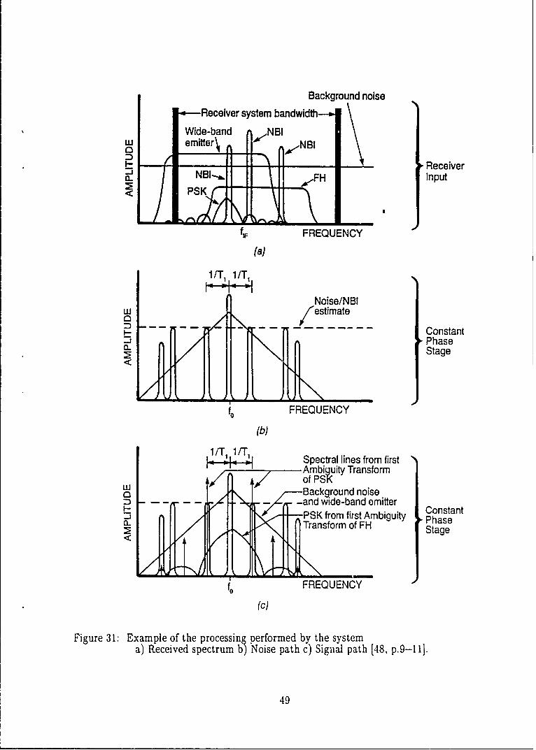
Background noise

Receiver system bandwidth

Wide-band NBIuw emitter\ INBI

----- Receiver(L NBI= ,FH Input

f FREQUENCY

(a)

Noise/NBIWL estimateMI- Constant_ L Phase. Stage

fo FREQUENCY

(b)

1Spectral lines from firstLy Ambig3uity Transformof PSK

W , -Background noise0

... .-, - -and wide-band omitter__. Constant" -PSK from first Ambiguity PhasenL Transform of FH2<,,"" Stage

oll

fo FREQUENCY

(c)

Figure 31: Example of the processing performed by the systema) Received spectrum b) Noise path c) Signal path [,48, p.9 -11].

49

The system is basically made by cascading N similar stages. Stage 1 detectsConstant-Phase modulation schemes (M-PSK); stage 2 for Linear-Phase (M-FSK); andstage 3 for Quadratic-Phase signal (linear FM or chirp). Higher order phase modulationscould be implemented. The system performs classification by characterizing the phase.This hardware could not be modified for analog modulation types.

In Figure 30, the signal 22 comes from the preceeding stage, and signal 22L goes tothe following stage. Signals 31L and 26L are used by the decision circuits. The systemperforms signal detecticn and classification. Therefore, it allows more than one modulationtype in the bandwidth of iDterest. The system would also work in the presence ofinterfering signals.

Figure 31-a shows an example of a received spectrum where several modulationtypes are present. The detection of a constant-phase signal, in the example PSK, would beperformed by stage 1. The output of the first stage noise path envelope detector is anestimation of the noise amplitude. This threshold value is used to detect the presence of asignal at the output of the first stage signal path envelope detector. Figure 31-c, presentsthat output. We can see the same spectrum as 31-b but with two additional narrowspectral lines above the noise threshold. These spectral lines are symmetric about thecarrier frequency and indicate the presence of a constant-phase signal and its symbol rate.The last path, i.e. the phase extractor, gives information on the phase difference betweenthe clock circuit and the data clock of the received signal.

5.2 KIM APPROACH

Kim [49][50] presented his energy detector as a way to classify phase-modulatedsignals. Using only one feature, i.e. qLLR defined below, he was able to discriminateBPSK from QPSK for very low SNR (0dB). The algorithm is as follows:

qLLR - (E - )2 + 4Q

where all E are energy related and defined by

N N N

Q n; E In Qn

nI n=I nI

nT

r, r(t)coswct d.; n=l,...,N(n-I)T

nT

rq,, - r(t)sinw t dt; n=l,...,NQ,i- I) T

and r (t' is the received signal containing AWGN.

50

The feature proposed seems to perform well with AWGN. The results are given forSNRs as low as 0dB with close to 100% correct classification. However, Kim assumed aprecise knowledge of the carrier frequency and symbol timing. In a real system, accuratedeterminations of these might be very difficult for signals as noisy as 0 dB, and might leadto unfortunate performance degradations. Moreover, it is not dear that the system will notreact to other modulat:on schemes that might be presented to the Modulation RecognitionSub-System in a real system. This technique is applicable only to digital phasemodulation schemes.

5.3 GARDNER APPROACH

Gardner is well known in the energy detection area. In a paper [51] he proposed theuse of his techniques for modulation classification purposes. The interception of LPI signalis accomplished by exploiting cyclic features which are present in modulated signals:sinewave carrier, data rate, etc.. The theory of spectral correlation in cyclostationarysignals developed by Gardner has been shown to be a general and flexible cyclic featureestimator called a cyclic spectrum analyser.

The process maps a time varying signal (2-D) into a 3-D distribution, using cyclicspectra. The distribution presents some characteristic shapes potentially useful formodulation classification.

The time varying signal 4 t) is cyclostationary if the parameter

R.(r) = lim - r4t+r/2)x(t-,r/2)ei 2 atdtT-sw T J-T/2

is not zero for some a 1 0. R(r) is called the cyclic autocorrelation, and its Fouriertransform is called the cyclic spectrum, S..(j), and can be interpreted as a spectralcorrelation function via the following characterization.

= I im Iim A t X 1 tf+a/2)Xr'(t,f-a/2)dtT-w At--u TA -At/2

t-T/2

The set {a: R'(r) f 0} is called the set of cycle frequencies. Some examples arepresented in Figure 32.

51

IZ (I

-5/Tr= f 0ro Or

(a) (c)

00

5/To10/1 /To I 5/T/1 T

f f

(b) (d)

Figure 32: Theorical spectral correlation distributions [52, p. 902]a) BPSK b) QPSK c) OQPSK d) MSK

These distributions show some discriminating power among modulation types.However, Gardner did not discuss how these distributions are sensitive to parameters suchas baud rate, modulation index, carrier frequency, etc.. Neither did he discuss the abilityof his cyclic feature to characterize analogue modulations regarding the random nature ofvoice (a nonstationary process). The potential advantage of this tethnique is its ability torecognize a modulated signal in the presence of interference.

52

6.0 CONCLUSION

In this document, we have seen how different authors have performed modulationrecognition. Using pattern recognition techniques, they have implemented a classificationalgorithm able to associate features, which have been judged discriminative, to differentclasses according to the similarity between the unknown pattern vector and the referencepattern vectors obtained during the training.

For the classification process, it seems that the linear and the binary tree classifierhave been adopted almost unanimously. The linear classifier is the simplest of parametrictechniques. Using only the pooled within-class covariance matrix to classify the unknownsignal, this technique is very fast and easily implemented. For a real-time requirementsuch as MR, it is a good choice. However, for solving bigger problems, with numerousclasses and features, it is usually advantageous to use more sophisticated algorithms. Thequadratic classifier, by using parabolic functions instead of linear ones to discriminateclusters, could, depending upon the particular application, present improved performanceThe outcome is an additional amount of memory and computation time for manipulatingthe within-class covariance matrices (one per class).

Although these parametric techniques could be optimal in some applications(typically when the distributions are normal), the more general case of non-parametrictechniques sometimes needs to be investigated (for example, when distributions aremulti-modal). In this technical note, only the binary tree concept has been discussed.Modern algorithms for creating trees are very powerful for handling a large amount ofclasses and features. The CART algorithm is probably the most standard type.

Notice that there also exists other nonparametric algorithms in classicalpattern-recognition literature [15]. Kernel (Parzen estimator) and K-nearest-neighborapproaches are very well known. In the first case, the density function, instead ofassumedly being known as in the parametric approach, is approximated by a sum ofkernels. These can be any functions, although normal kernels are usually used. Forclassification, the unknown signal is compared to all N training samples according to thethe kernel function in use and is associated to the closest class considering the overallprobability. For the K-nearest-neighbor, the decision rule is simplified by consideringonly the K samples closest to the unknown (instead of all N samples) to compute theprobabilities p(w, I z). Unfortunately it is still necessary to store all N samples and comparethe unknown with all these samples to find the K closest points. Therefore, the amount ofcomputation is not significantly decreased. In order to overcome this disadvantage, itwould be interesting to eliminate samples, keeping only some good representative3 (locatedalong boundaries). This process is called condensed K-nearest-neighbor decision rule in(15].

Another alternative, not proposed by the authors mentioned in this paper, but verypopular in modern pattern recognition research centers, could also be applied to the MRproblem. Neural networks are very interesting nonparametric techniques which provideefficiency and extreme versatility with numerous applications. The great interest for thisartificial brain is fairly new but some algorithms are becoming well established, such as theback-propagation network. It is highly likely that some new MR systems will use neuralnetworks, in the future, when neural network VLSIs will be available on the market.

53

Although the choice of the classifier is very important, the selection of good featuresis fundamental. The features have to be discriminative, noise resistant and requiring asfew computation as possible. A feature is obtained from the probability distribution(histogram) of a parameter, which is usually computed on a point to point basis from thesampled signal waveform. Popular parameters are the signal envelope, the instantaneousfrequency, etc. Some authors also used the frequency distribution (PSD) to represent theparameter. In both cases, the features are chosen in order to represent efficientlycharacteristics from the distribution. Very often the mean and standard deviation areused, although the skewness and the kurtosis are also popular (Einicke and Hipp). Anotherapproach consists of using directly the bin values of the distribution as features (Jondral).Unfortunately the latter gives rise to a very large dimension feature vector. To avoid thatproblem, only the most significant bins can be used: Miller used the first bin, p(O), fromthe signal envelope distribution. See Table 6 for more examples.

Section Author Parameter Time/Freq Feature

3.1 Miller Signal Envelope A T Bin value p(O)

3.2 Gadbois A2 T

(A2)2

Gallant A2 T O(a 2(A 2 ))

3.3 Fabrizi Instant. Freq. F, T (F)

3.4 Aisbett A2Fi T

AN T I

3.5 Hipp PSD(signal R) F a (PSD(R))

PSD(signal2) F a(PSD(R2))

4.1 Jondral A, F, and F,' T Bin values

Table 6: Examples of features used for modulation recognition

54

It would be interesting at this time to investigate a stepwise selection of thesefeatures to get a discriminative pattern performing with noisy signals and short acquisitiontimes. Some new features would also be very desirable, features able to deal with lowerSNRs, shorter acquisition times, and more modulation types. From a military perspective,classification of signals with SNRs as low as 5 to 10 dB presents a real interest. Gallant'ssolution of very long acquisition time (a little below 2 seconds) to remove gaps in the voiceis not adequate for all applications. A new feature able to discriminate analoguemodulation types with a shorter acquisition time would be very desirable. Finally it wouldbe worthwhile to be able to recognize other power-efficient modulation types such as MSK,OQSPK, GMSK and TFM.

55

REFERENCES

[1] S. Faulkner, "CERES - A Computer-Aided Radio Monitoring and SurveillanceSystem", International Defense Review: An Interavia Publication", June 1977.

[2] Liedtke, F.F., "Computer Simulation of an Automatic Classification Procedure forDigitally Modulated Communication Signals with Unknown Parameters", SignalProcessing, Vol.6, 1984.

[3] Gallant, M.J., "Modulation Recognition", Royal Military College, Kingston, ONT.,April 1989.

[4] DeSimio, Martin P., "Automatic Classification of Digitally Modulated Signals", AirForce Inst of Technology, Wright-Patterson Air Force Base, Ohio, December 1987.

[5] DeSimio, Martin P. et al., "Adaptive Generation of Decision Functions forClassification of Digitally Modulated Signals", NAECON, 1988.

[6] Einicke,G.A., "A Flexible Architecture for Real-Time Modulation Recognition",Communications Div., Electronics Research Laboratory, Salisbury, S.A.

[7] Fry, Robert, "Modifications to a Spectrum Surveillance Electronic Support Measure(ESM) Receiver Developed for the Department of National Defence (U)", TechnicalNote 85-7, Defence Research Establishement Ottawa, March 1985.

[8] Hipp, Jackie E., "Modulation Classification Based on Statistical Moments",MILCOM'86, pp.20.2.1-20.2.6.

[9] Ribble, C.S., "Automatic Modulation Recognition", Royal Military College,Kingston, Ontario, April 1987.

(10] Mammone, R.J., et al., "Estimation of Carrier Frequency, Modulation Type and BitRate of an Unknown Modulated Signal", Proc. of the ICC, 1987.

[11] Julius T. Tou and Rafael Gonzalez, "Pattern Recognition Principles",Addison-Wesley, 1974

[12] Richard P. Lippman, "Pattern Classification Using Neural Networks", IEEECommunications Magazine, November 1989, pp.47-64.

[13] Mich~le Basseville, "Distance Measures for Signal Processing and PatternRecognition", Signal Processing, December 1989, pp.349-369.

[14] Afifi, A.A. and Clark, Virginia, "Computer-Aided Multivariate Analysis", LifetimeLearning Publications, Belmont, California, 1984.

[15] K. Fukunaga, "Introduction to Statistical Pattern Recognition", Academic Press,1972.

REF-1

[16] Josef Kittler, "Mathematical Methods of Feature Selection in Pattern Recognition",International Journal of Man-Machine Studies, Vol.7, 1975, pp.609-6 37.

[17] R. A. Fisher, "The Use of Multiple Measurements in Taxonomic Problems", Annalsof Eugenics, 7:179-188, 1936

[18] Tzay Y. Young, "Handbook of Pattern Recognition and Image Processing",Academic Press, 1986.

[19] Seymour Shlien, "Nonparametric Classification Using Matched Binary DecisionTree", to appear in Pattern Recognition Letters, 1990.

[20] Gerard T. LaVarnway, "An Introduction to CART: Classification and RegressionTrees", in "Computing Science and Statistics", Proceeding of the 20th Symposiumon the Interface, Fairfax, Virginia, April 1988, edited by E.J. Wegman et al..

[21] Watkins-Johnson Company, "WJ-8607 VHF/UHF Surveillance Receiver,Developmental Specification", Watkins-Johnson Company, Gaithersburg, Md.,Change 2, January 1988.

[22] Winkler, C., "The Operation of an Advanced Modulation Recognition Algorithm",Technical Memorandum ERL-0i85-TM, Electronics Research Laboratory, DefenceResearch Centre, Salisbury, Australia, February 1981.

[23] Calian Communications Systems Limited, "Feasibility Study for a HF/VHF ESMReceiver", Miller Communications Systems Limited, Kanata, Ontario, Canada,January 1978.

[24] Calian Communications Systems Limited, "Development of a Spectrum SurveillanceElectronic Support Measures Receiver System-Operators Manual and Test Report",DSS Contract #2SR79-00069, MCS File #7829 PR/ce, Miller CommunicationsSystems Limited, Kanata, Ontario, Canada, October 1980.

[25] Calian Communications Systems Limited, "The ESM Receiver Operator's Manualand Test Report", Miller Communications Systems Limited, Kanata, Ontario,Canada, January 1981.

[26] Calian Communications Systems Limited, "Frequency Resolution AlgorithmSelection for Improved Identification Performance in the CAIR Receiver", MCS FileNo.8136, Miller Communications Systems Limited, Kanata, Ontario, Canada,November 1982.

[27i Calian Communications Systems Limited, "Operating Manual Intercept Receiver",CS File No.8136, Calian Communications Systems Limited, Kanata, Ontario,Canada, February 1983.

[28] Jondral, Friedrich, "Aultomatic Classification of High Frequency Signals", SignalProcessing, Vol.9, 1985.

REF-2

[29] Jondral, Friedrich, "Foundations of Automatic Modulation Classification",Stochastische Modelle und Methoden in der Informationstechnik, AEGAktiengesellschaft, April 1989.

[30] Torrieri, D.J., "Principles of Military Communication Systems", Artech House,Massachusetts, 1981, p.11.

[31] Luiz, R., "HF/VHF Spectrum Surveillance ESM Receiver", Department of NationalDefence Canada, Ottawa, Technical Note No. 81-17, September 1981.

[32] Wakeman, Philip E.D., "Spectrum Surveillance Receiver System", US Patent4,501,020, 19th February 1985.

[331 Gadbois, L.G. et al., "Identification of the Modulation Type of a Signal", IEEEInternational Conference on Acoustics, Speech, and Signal Processing, March 1985.

[34] Gadbois, L.G., "Modulation Identification", Royal Military College, Kingston,ONT., October 1985.

[351 Gadbois, L.G. et al., "Identification of the Modulation Type of a Signal", SignalProcessing, Vol.16, 1989.

[36] UTL CANADA INC., "HFSS Modulation Recognition Study", DND/DEEM 4Contract No. W8477-7-CC20/01-SV, August 1989.

[37] Weaver, C.S., et al., "The Automatic Classification of Modulation Types byPattern Recognition", Technical Report No. 1829-2, Stanford ElectronicsLaboratories, Stanford University, Stanford, CA, April 1969.

[38] Callaghan, T.G., et al., "Sampling and Algorithms Aid Modulation Recognition",Microwave & RF, September 1985.

[39] Fabrizi, P.M., et al., "Receiver Recognition of Analogue Modulation Types", IEREConference on Radio Receivers and Associated Systems, Bangor, Wales, 1986.

[40] Petrovic, P.M. et al., "An Automatic VHF Classifier" MediterraneanElectrotechnical Conference, MELECON'89.

[41] Aisbett, J., "A,.,tomatic Modulation Recognition Using Time Domain Parameters",Electronic Research Lab, Adelaide, Australia, Technical Report ERL-0367-TR,November 1986.

[42] Aisbett, Janet, "Automatic Modulation Recognition Using Time DomainParameters", Signal Processing, Vol.13, No.3, pp.323-328, 1987.

[43] Vergara-Dominguez, L., Portillo-Garcia, J., et al., "Modulated SignalClassification: A General Approach", Proc. of the IASTED InternationalSymposium, June 1987.

[44] Vergara-Dominjuez, L., Portillo-Garcia, J., et al., "A Radio CommunicationSignal Classifier' , EURASIP 1988, Signal Processing IV, pp.1361-1364, 1988.

REF-3

[451 Adams, E.R. et al., "A Statistical Approach to Modulation Recognition forCommunications Signal Monitoring and Surveillance", Fifth InternationalConference on Digital Processing of S-gnals in Communication, 1988.

[46] Tatsuoka, M., "Multivariate Analysis: Techniques for Educational andPsychological Research", Wiley, 1971.

[47] Richard P. Lippman, "An Introduction to Computing with Neural Nets", IEEEASSP Magazine, April 1987.

[48] Ready, Patrick J. et al., "Modulation Detector and Classifier", US Patent 4.597,107,24th June 1986.

[49] Kim, Kiseon and Polydoros, Andreas, "Modulation Detection/Classification forPhase-Modulated Digital Signals in Broadband Noise", Communication SciencesInstitute, Departement of Electrical Engineering, University of Southern California,Los Angeles, November 1987.

[50] Kim, Kiseon and Polydoros, Andreas,"Digital Modulation Classification: The BPSKversus QPSK case", MILCOM, 1988.

[51] Gardner, William A. et al., "Cyclic Spectral Analysis for Signal Detection andModulation Recognition", MILCOM, 1988.

[52] William A. Gardner, "Signal Interception: A Unifying Theorical Framework forFeature Detection", IEEE Transactions on Communications, Vol.36, No.8, August1988, pp.897-906.

REF-4

UNCLASSIFIED -61-SECURITY CLASSIFICATION OF FORM

(highest classification of Title, Abstact, Keywords)

DOCLMENT CONTROL DATA(Socurity Classificaltion of title, body of abstrlCt and ndexing anotation mulst be entered when the overall document is classified)

1. ORIGINATOR Ithe name and address of the orgauizauor, prooaring the dcument 2. SECURITY CLASSIFICATIONOrganizations for whom the docutmiti was prepared e.gS Es1ishmrt spcnsori": (overall security classificatin of the docunenta contractor's report, or tasking agency, we entered in section L) including special warning terms if applicable)

NATIONAL DEFENCEDEFENCE RESEARCH ESTABLISHMENT OTTAWASHIRLEY BAY, OTTAWA, ONTARIO KiA OZ4 CANADA UNCLASSIFIED

3. TITLE (the complete document title as indicated on the title Pge. ;ts classification Should be indicated by the appropriateabbreviation (S.C or U) in parentheses aftar the title.)

MODULATION RECOGNITION: AN OVERVIEW (U)

4. AUTHORS (LaST name, first name. middle initio)

'LAMONTAGNE, RENE

5. DATE OF PUBLICATION (month and year of publication of 6a NU. OF PAGES (total 6b NO OF REFS (total cited indocument) containing information. Include document)

Annexes. Appendices. etc.)MIARCH 91 68 56

7 DESCRIPTIVE NOTES (the category of the document. e.g. tecinical report, technical note or memorandum. If appropriate, enter the type ofreport, e.g. interim, progress, summary, annual or final. Give the inclusive dates when a specif,c reporting Period IS covered.)

DREO TECHNICAL NOTE 91-3

8. SPONSORING ACTIVITY (the name of the department project office or laboratory sponsoring the research and development. include theaddress.)

NATIONAL DEFENCEDEFENCE R<ESEARCH ESTABLISHfMENT OTTAWASHIRLE1 BAY, OTTAWAT. ONTARIO KIA OZ4 CANADA9a. PROJECT OR GRANT NO. (if appropriate, the applicable research 9b. CONTRACT NO (if appropriate, the applicable number unoer

and development orojuct or grant number under which the document which the document was wrinen)was written. Please specify whether project or gram)

041LKi

10a. ORIGINATOR'S DOCUMENT NUMBER (the official document 10b. OTHER DOCUMENT NOS. Any other numbers which maynumber by which the document is identified by the originating be assigned this document either oy the originator or by theactivity. This number must be unique to this document) sponsor)

DREO TECHNICAL NOTE 91-3

DOCUMENT AVAILABILITY (any limitations on further dissemination of the document, other than those imposec bv security ciassificationi

"X) Unlimited distribution

( I Distribution limited to defenci departments and defence contractors: further distribution only as aoprovedI I Distribution limited to deferat departments and Canadian defence contractors, further distribution oniy as aoproved

I Distribution limited to government departments and agencies: further distribution only as approvedI Distribution limited to defence departmens; further distribution only as approvedI Other (please specify):

12 DOCUMENT ANNOUNCEMvE'T (any limitation to the bibliograonic announcement o this document This wii, normally correSoond tothe Document Availabilty (11). However, where further distribution (beyond the audience specifieo n 11) is Possiole, a widerannouncement audience may be selected.)

UNCLASSIFIED

SECURITY CLASSIFICATION OF FORM

DCD0O 2,06'

-62- UNCLASSIFIEDSECURITY CLASSIFICATION OF FORM

13. ABSTRACT ( a trief and factual suAlaryj of the diaarnet it may also apea elsewhere in the body of the document itself It is highlyoesirale that the abstract of classif ied doculments be unclassified. Each Wagroph of the abstract shall bein with an indication of thesecurity clossdfecation of mhe information in the WWy~h (unless mhe document itself is unclassified) represented as IS). X)?. or (U).It is not necessary t6 include here abstracts in both off" icL lwgos unless the text is bilingual).

THE NTEr-EST FOR A SYSTEM ABLE TO AUTOMATICALLY IDENTIFY THE MODULATIO)N TYPEOF MN INTERCEPTED RADIO SIGNAL IS INCREASINGLY EVIDENT FOR MILITARY AND CIVILIANPURPOSES. ALTHOUrH I.1 THE PAST SOHE AUTHORS LOOKED AT THE 1ROBLE.'f,NOBlODY F0U-;J "iiz~SOLUTION" AND THE PROBLE:4 RE'!AIN.S. THEREFORE, Ai OVE21VIM! 0-- MiE PROPI)SED £ZCH.IUESIS USEFUL IN ORDER TO ASSESS THE ACTUAL SITUATION.

THIS DOCLU1ENT PRESENTS CLASSIFICATIO)N TECHNTIOUES AND FEATURES (PARAMETERSCHIARACTERIZING THE MODULATION TYPES) USED FOR MODULATION RECOGNITION.

O.UE CE SOIT POUR DES FINS MILITAIRES OU CIVILES, L'INTERtT D'UNE MACHI.;ECAPABLE D'IDENTIFIER AUTOMATIO.UEME:T LE TYPE DE MODULATION D' UN SIGNAL INCO.NNu ZSTEVIDENT. DIEN QUE PAR LE PASSE CERTAINS AUTEURS SE SOIEN.T PENCHES SUR LE PROBLE'IE,PERSONNE N 'A OBTE.4UE D' ECLATANT RESULTATS INDIOCANT LA ROUTE A SUIVU.E. PAR 2NEU11L N'Y A PAS LIEU DE CO.;CENTRER SES EFFORTS SUR UN SEUL AUTEUR MAIS SUR L'ENSE'IBLE ILSTECIEIIQUES PROPOSEES.

CE DOCUMENT COUVRE DONC LE SUJET D'UNE FACON GLOBALE, PRESETTANT LES TECHII:IU'TEFPWIR CLASSIFICATION AINSI QUE LES PAPMETRES UTILISES POUR CARACTERISER ET DIST! WELES DIVERS TYPES DE MODULATION, TEL OUE PROPOSES PAR LES AUTEURS.

4 14ET'ORDS. OESCRIPTORS or IDENTIFIERS (technically meaningful terms or short Phrases thit characterize a toccument aria cuid tieheipful -n cataloguing the document They should be selected so that no security classification ~s *eauirea. mentifiers, sucr as eouior'lenymoce oesignatuazn. trade name. military project code name. geographic location may also be incivoed If Possibie keywords shouc be seieceltrom a oubliised thesaurus. e.g. Thesaurus of Engineering ano Scientific Terms (TEST) and that thesaurus-'oentfea s n o' Oo,.C *0select indexing terms winich are Unclassified, the classification of each snould be indicated as with the :itle.)

MODULATION RECOGNITIONMODULATION CLASSIFICATIONMODULATION IDENTIFICATION

SECURITY CLA SIFVCAT ON OF FORM