agresti/franklin statistics, 1 of 82 chapter 13 comparing groups: analysis of variance methods learn...
TRANSCRIPT
Agresti/Franklin Statistics, 1 of 82
Chapter 13Comparing Groups: Analysis of
Variance Methods
Learn …. How to use Statistical inference
To Compare Several Population
Means

Agresti/Franklin Statistics, 2 of 82
Section 13.1
How Can We Compare Several Means?
One-Way ANOVA
Agresti/Franklin Statistics, 3 of 82
Analysis of Variance
The analysis of variance method compares means of several groups
• Let g denote the number of groups
• Each group has a corresponding population of subjects
• The means of the response variable for the g populations are denoted by µ1, µ2, … µg

Agresti/Franklin Statistics, 4 of 82
Hypotheses and Assumptions for the ANOVA Test
The analysis of variance is a significance test of the null hypothesis of equal population means:
• H0: µ1 = µ2 = …= µg
The alternative hypothesis is:
• Ha: At least two of the population means are unequal
Agresti/Franklin Statistics, 5 of 82
Hypotheses and Assumptions for the ANOVA Test
The assumptions for the ANOVA test comparing population means are as follows:
1.The population distributions of the response variable for the g groups are normal with the same standard deviation for each group
Agresti/Franklin Statistics, 6 of 82
Hypotheses and Assumptions for the ANOVA Test
2.Randomization:
• In a survey sample, independent random samples are selected from the g populations
• In an experiment, subjects are randomly assigned separately to the g groups

Agresti/Franklin Statistics, 7 of 82
Example: How Long Will You Tolerate Being Put on Hold?
An airline has a toll-free telephone number for reservations
The airline hopes a caller remains on hold until the call is answered, so as not to lose a potential customer
Agresti/Franklin Statistics, 8 of 82
Example: How Long Will You Tolerate Being Put on Hold?
The airline recently conducted a randomized experiment to analyze whether callers would remain on hold longer, on the average, if they heard:
• An advertisement about the airline and its current promotion
• Muzak (“elevator music”)
• Classical music
Agresti/Franklin Statistics, 9 of 82
Example: How Long Will You Tolerate Being Put on Hold?
The company randomly selected one out of every 1000 calls in a week
For each call, they randomly selected one of the three recorded messages
They measured the number of minutes that the caller stayed on hold before hanging up (these calls were purposely not answered)

Agresti/Franklin Statistics, 10 of 82
Example: How Long Will You Tolerate Being Put on Hold?
Agresti/Franklin Statistics, 11 of 82
Example: How Long Will You Tolerate Being Put on Hold?
Denote the holding time means for the populations that these three random samples represent by:
• µ1 = mean for the advertisement
• µ2 = mean for the Muzak
• µ3 = mean for the classical music
Agresti/Franklin Statistics, 12 of 82
Example: How Long Will You Tolerate Being Put on Hold?
The hypotheses for the ANOVA test are:
• H0: µ1=µ2=µ3
• Ha: at least two of the population means are different
Agresti/Franklin Statistics, 13 of 82
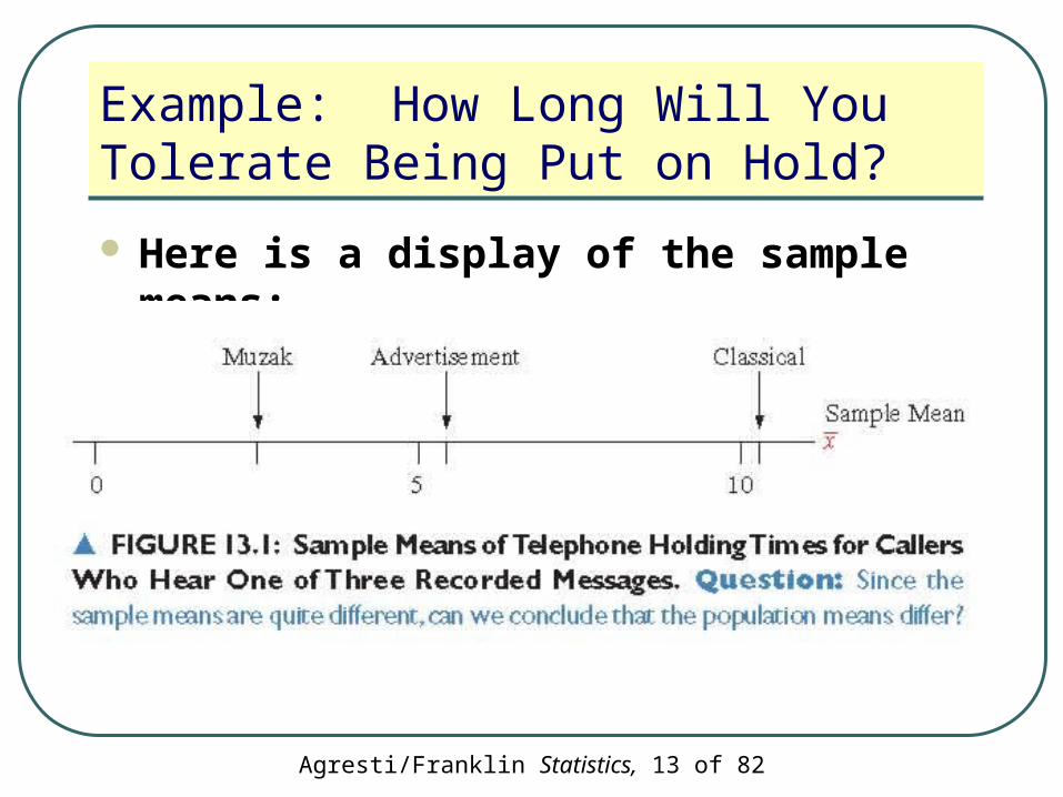
Example: How Long Will You Tolerate Being Put on Hold?
Here is a display of the sample means:
Agresti/Franklin Statistics, 14 of 82
Example: How Long Will You Tolerate Being Put on Hold?
As you can see from the graph on the previous page, the sample means are quite different
This alone is not sufficient evidence to enable us to reject H0
Agresti/Franklin Statistics, 15 of 82
Variability between Groups and within Groups
The ANOVA method is used to compare population means
It is called analysis of variance because it uses evidence about two types of variability
Agresti/Franklin Statistics, 16 of 82
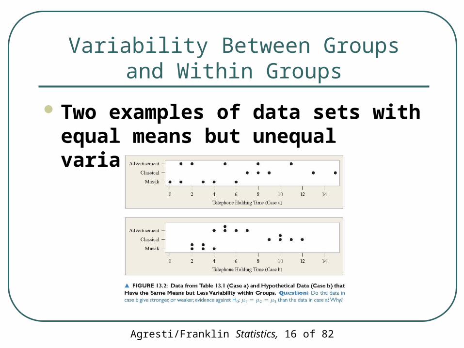
Variability Between Groups and Within Groups
Two examples of data sets with equal means but unequal variability:

Agresti/Franklin Statistics, 17 of 82
Variability Between Groups and Within Groups
Which case do you think gives stronger evidence against H0:µ1=µ2=µ3?
What is the difference between the data in these two cases?
Agresti/Franklin Statistics, 18 of 82
Variability Between Groups and Within Groups
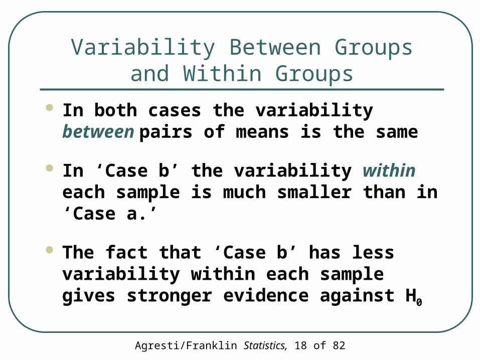
In both cases the variability between pairs of means is the same
In ‘Case b’ the variability within each sample is much smaller than in ‘Case a.’
The fact that ‘Case b’ has less variability within each sample gives stronger evidence against H0
Agresti/Franklin Statistics, 19 of 82
ANOVA F-Test Statistic
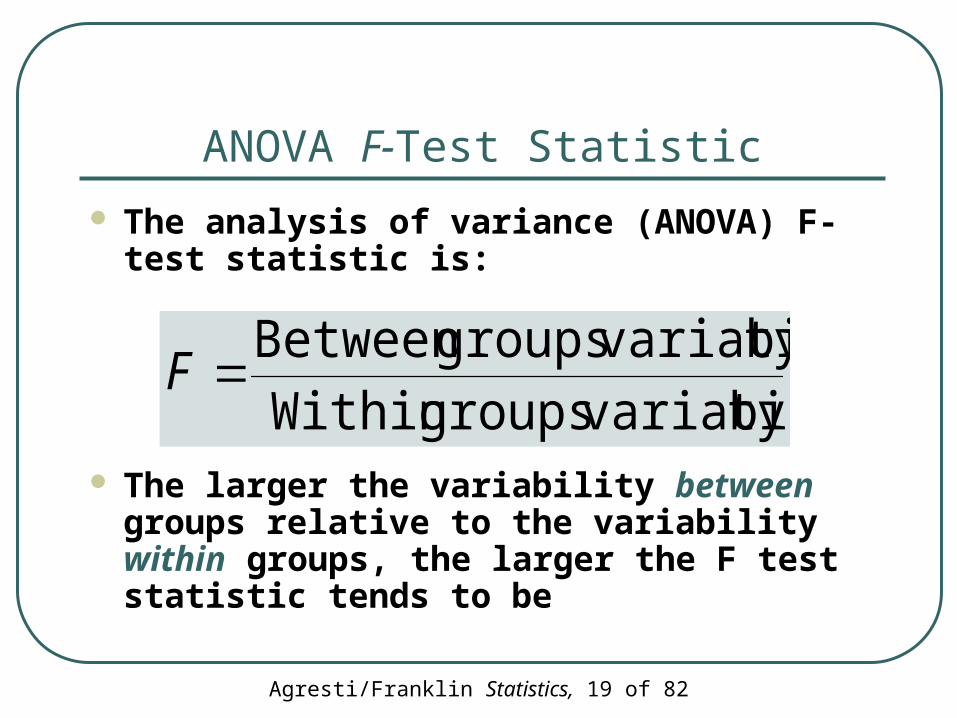
The analysis of variance (ANOVA) F-test statistic is:
The larger the variability between groups relative to the variability within groups, the larger the F test statistic tends to be
ty variabiligroupsWithin
ty variabiligroupsBetween F

Agresti/Franklin Statistics, 20 of 82
ANOVA F-Test Statistic
The test statistic for comparing means has the F-distribution
The larger the F-test statistic value, the stronger the evidence against H0
Agresti/Franklin Statistics, 21 of 82
ANOVA F-test for Comparing Population Means of Several Groups
1. Assumptions: Independent random samples
Normal population distributions with equal standard deviations
Agresti/Franklin Statistics, 22 of 82
ANOVA F-test for Comparing Population Means of Several Groups
2. Hypotheses:
• H0:µ1=µ2= … =µg
• Ha:at least two of the population means are different

Agresti/Franklin Statistics, 23 of 82
ANOVA F-test for Comparing Population Means of Several Groups
3. Test statistic:
F- sampling distribution has df1= g -1, df2 = N – g = (total sample size – no. of groups)
ty variabiligroupsWithin
ty variabiligroupsBetween F
Agresti/Franklin Statistics, 24 of 82
ANOVA F-test for Comparing Population Means of Several Groups
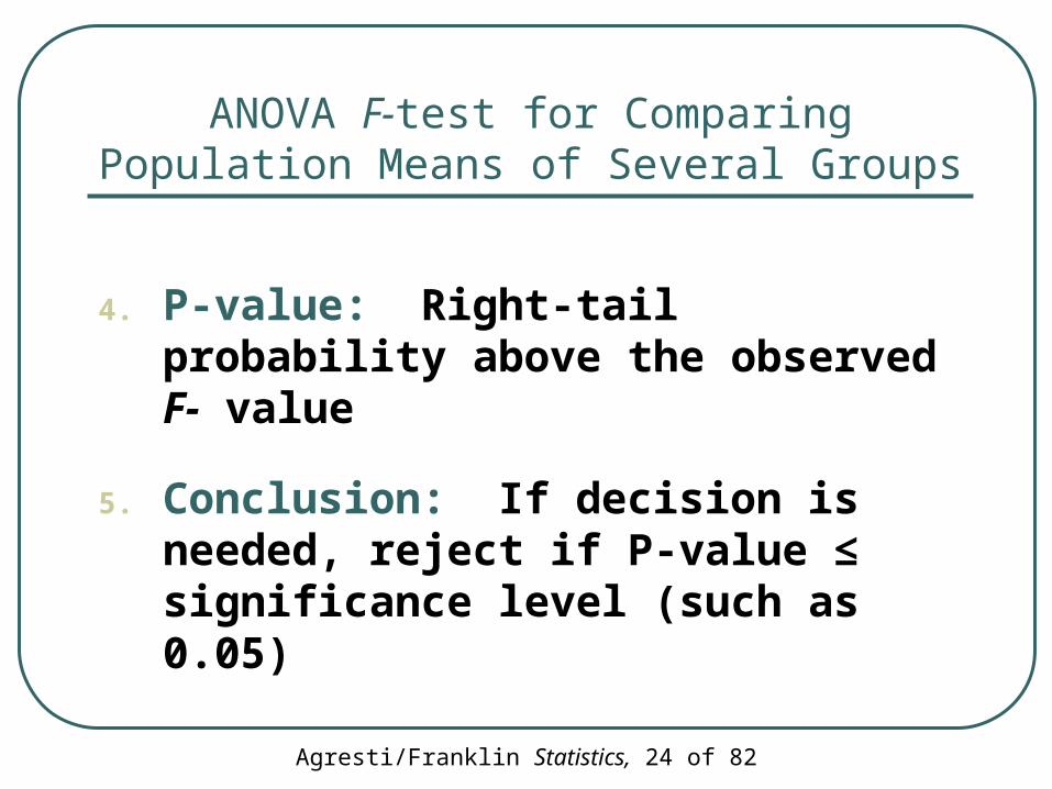
4. P-value: Right-tail probability above the observed F- value
5. Conclusion: If decision is needed, reject if P-value ≤ significance level (such as 0.05)
Agresti/Franklin Statistics, 25 of 82
The Variance Estimates and the ANOVA Table
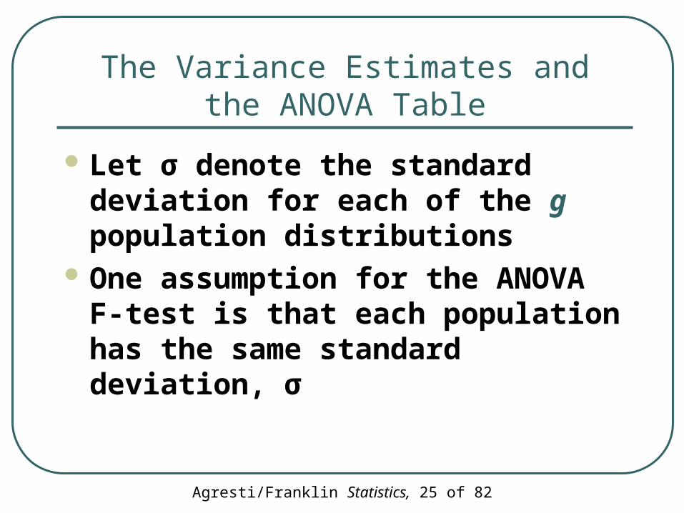
Let σ denote the standard deviation for each of the g population distributions
One assumption for the ANOVA F-test is that each population has the same standard deviation, σ

Agresti/Franklin Statistics, 26 of 82
The Variance Estimates and the ANOVA Table
The F-test statistic is the ratio of two estimates of σ2, the population variance for each group
The estimate of σ2 in the denominator of the F-test statistic uses the variability within each group
The estimate of σ2 in the numerator of the F-test statistic uses the variability between each sample mean and the overall mean for all the data
Agresti/Franklin Statistics, 27 of 82
The Variance Estimates and the ANOVA Table
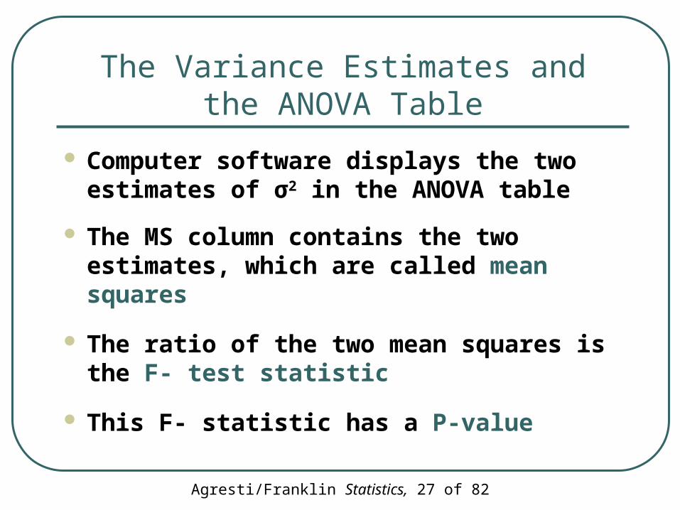
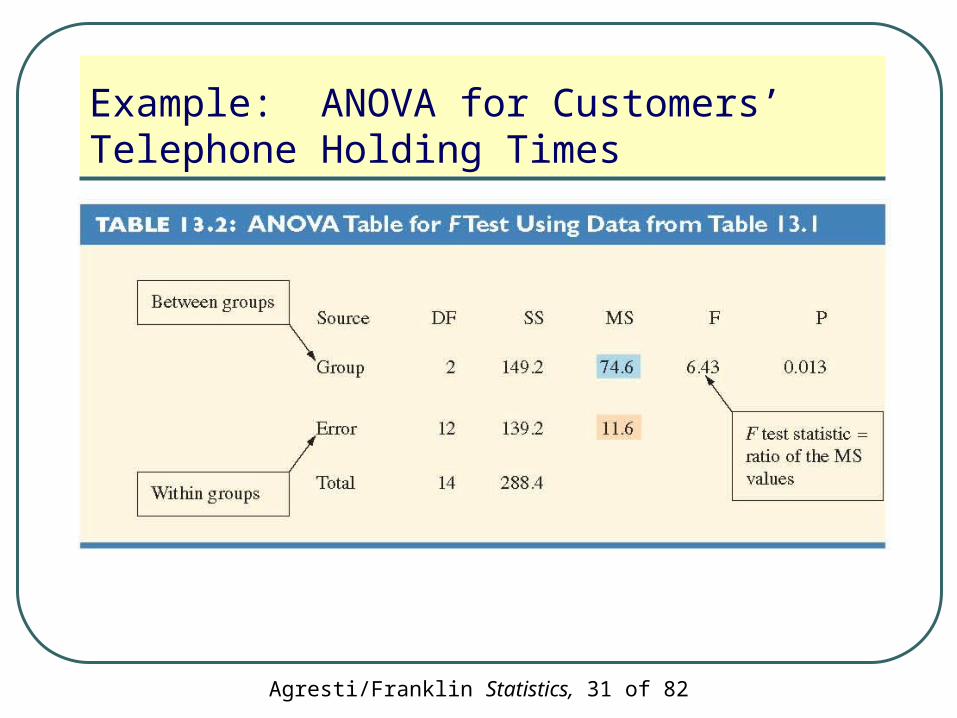
Computer software displays the two estimates of σ2 in the ANOVA table
The MS column contains the two estimates, which are called mean squares
The ratio of the two mean squares is the F- test statistic
This F- statistic has a P-value

Agresti/Franklin Statistics, 28 of 82
Example: ANOVA for Customers’ Telephone Holding Times
This example is a continuation of a previous example in which an airline conducted a randomized experiment to analyze whether callers would remain on hold longer, on the average, if they heard:• An advertisement about the airline and its
current promotion
• Muzak (“elevator music”)
• Classical music
Agresti/Franklin Statistics, 29 of 82
Example: ANOVA for Customers’ Telephone Holding Times
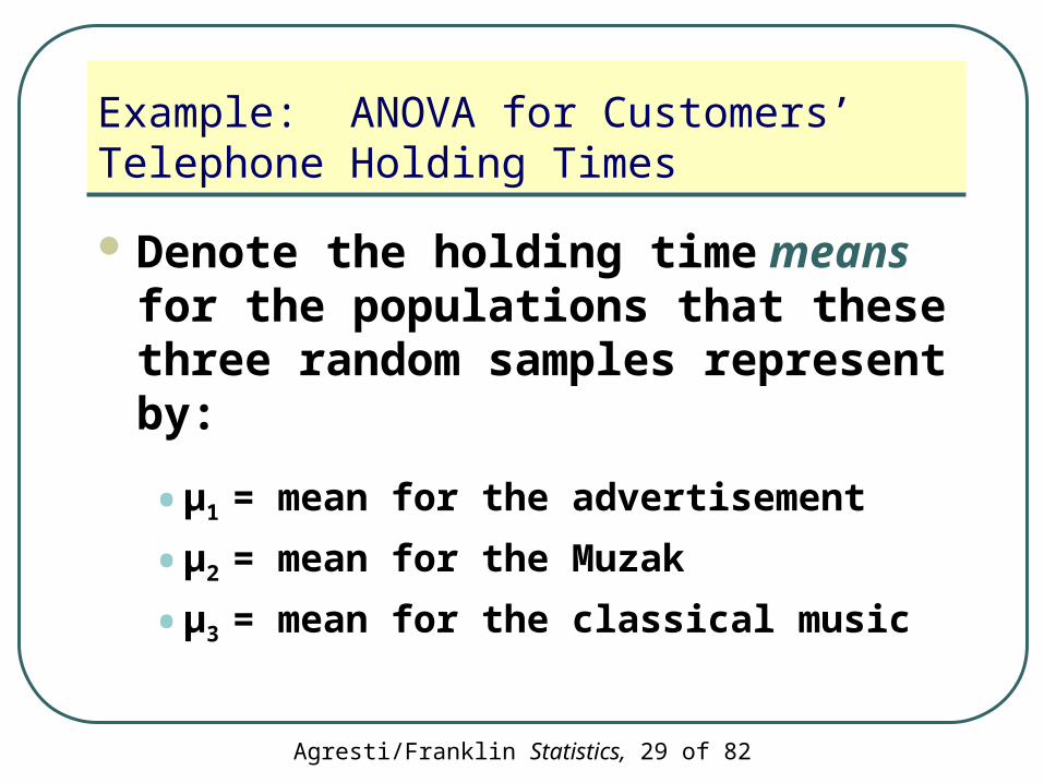
Denote the holding time means for the populations that these three random samples represent by:
• µ1 = mean for the advertisement
• µ2 = mean for the Muzak
• µ3 = mean for the classical music

Agresti/Franklin Statistics, 30 of 82
Example: ANOVA for Customers’ Telephone Holding Times
The hypotheses for the ANOVA test are:
• H0:µ1=µ2=µ3
• Ha:at least two of the population means are different
Agresti/Franklin Statistics, 31 of 82
Example: ANOVA for Customers’ Telephone Holding Times

Agresti/Franklin Statistics, 32 of 82
Example: ANOVA for Customers’ Telephone Holding Times
Since P-value < 0.05, there is sufficient evidence to reject H0:µ1=µ2=µ3
We conclude that a difference exists among the three types of messages in the population mean amount of time that customers are willing to remain on hold

Agresti/Franklin Statistics, 33 of 82
Assumptions for the ANOVA F-Test and the Effects of Violating Them
1. Population distributions are normal• Moderate violations of the normality
assumption are not serious
2. These distributions have the same standard deviation, σ• Moderate violations are also not serious
Agresti/Franklin Statistics, 34 of 82
Assumptions for the ANOVA F-Test and the Effects of Violating Them
You can construct box plots or dot plots for the sample data distributions to check for extreme violations of normality
Misleading results may occur with the F-test if the distributions are highly skewed and the sample size N is small

Agresti/Franklin Statistics, 35 of 82
Assumptions for the ANOVA F-Test and the Effects of Violating Them
Misleading results may also occur with the F-test if there are relatively large differences among the standard deviations (the largest sample standard deviation being more than double the smallest one)
Agresti/Franklin Statistics, 36 of 82
The 1998 General Social Survey asked subjects how many friend they have. Is this associated with the respondent’s astrological sign (the 13 symbols of the Zodiac)? The ANOVA table for the data reports F=0.61
State the null hypothesis
a. The population means for all 12 Zodiac signs are the same.
b. At least two population means are different.
Agresti/Franklin Statistics, 37 of 82
The 1998 General Social Survey asked subjects how many friend they have. Is this associated with the respondent’s astrological sign (the 13 symbols of the Zodiac)? The ANOVA table for the data reports F=0.61
State the alternative hypothesis
a. The population means for all 12 Zodiac signs are the same.
b. At least two population means are different.

Agresti/Franklin Statistics, 38 of 82
The 1998 General Social Survey asked subjects how many friend they have. Is this associated with the respondent’s astrological sign (the 13 symbols of the Zodiac)? The ANOVA table for the data reports F=0.61
Based on what you know about the F distribution would you guess that the test value of 0.61 provides strong evidence against the null hypothesis?
a. Nob. Yes
Agresti/Franklin Statistics, 39 of 82
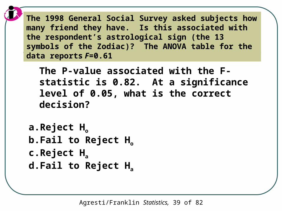
The 1998 General Social Survey asked subjects how many friend they have. Is this associated with the respondent’s astrological sign (the 13 symbols of the Zodiac)? The ANOVA table for the data reports F=0.61
The P-value associated with the F-statistic is 0.82. At a significance level of 0.05, what is the correct decision?
a. Reject Ho
b. Fail to Reject Ho
c. Reject Ha
d. Fail to Reject Ha
Agresti/Franklin Statistics, 40 of 82
Section 13.2
How Should We Follow Up an ANOVA F-Test?
Agresti/Franklin Statistics, 41 of 82
Follow Up to an ANOVA F-Test
When an analysis of variance F-test has a small P-value, the test does not specify which means are different or how different they are
We can estimate differences between population means with confidence intervals

Agresti/Franklin Statistics, 42 of 82
Confidence Intervals Comparing Pairs of Means
For two groups i and j, with sample means yi and yj having sample sizes ni and nj, the 95% confidence interval for µi - µj is:
The t-score has df = N – g
ji
ji nnstyy
11025.

Agresti/Franklin Statistics, 43 of 82
Confidence Intervals Comparing Pairs of Means
Some software refers to this confidence method as the Fisher method
When the confidence interval does not contain 0, we can infer that the population means are different
The interval shows just how different the means may be
Agresti/Franklin Statistics, 44 of 82
Example: Number of Good Friends and Happiness
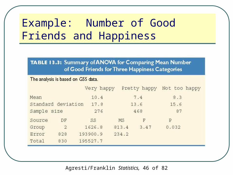
A recent GSS study asked: “About how many good friends do you have?”
The study also asked each respondent to indicate whether they were ‘very happy,’ ‘pretty happy,’ or ‘not too happy’

Agresti/Franklin Statistics, 45 of 82
Example: Number of Good Friends and Happiness
Let the response variable y = number of good friends
Let the categorical explanatory variable x = happiness level
Agresti/Franklin Statistics, 46 of 82
Example: Number of Good Friends and Happiness
Agresti/Franklin Statistics, 47 of 82
Example: Number of Good Friends and Happiness
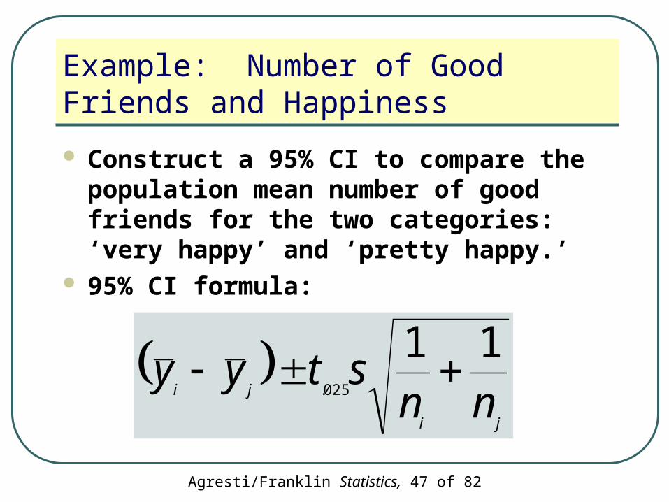
Construct a 95% CI to compare the population mean number of good friends for the two categories: ‘very happy’ and ‘pretty happy.’
95% CI formula:
ji
ji nnstyy
11025.
Agresti/Franklin Statistics, 48 of 82
Example: Number of Good Friends and Happiness
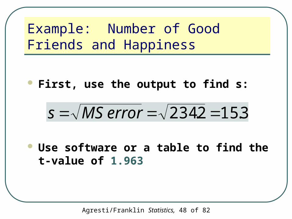
First, use the output to find s:
Use software or a table to find the t-value of 1.963
3.152.234 errorMSs
Agresti/Franklin Statistics, 49 of 82
Example: Number of Good Friends and Happiness
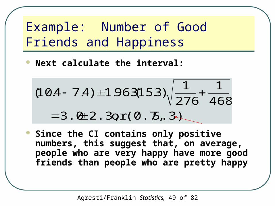
Next calculate the interval:
Since the CI contains only positive numbers, this suggest that, on average, people who are very happy have more good friends than people who are pretty happy
5.3) (0.7,or 2.3,3.0 468
1
276
1)3.15(963.1)4.74.10(
Agresti/Franklin Statistics, 50 of 82
Controlling Overall Confidence with Many Confidence Intervals
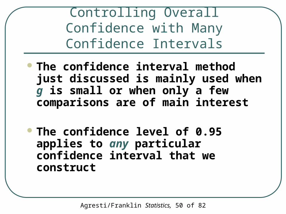
The confidence interval method just discussed is mainly used when g is small or when only a few comparisons are of main interest
The confidence level of 0.95 applies to any particular confidence interval that we construct
Agresti/Franklin Statistics, 51 of 82
Controlling Overall Confidence with Many Confidence Intervals
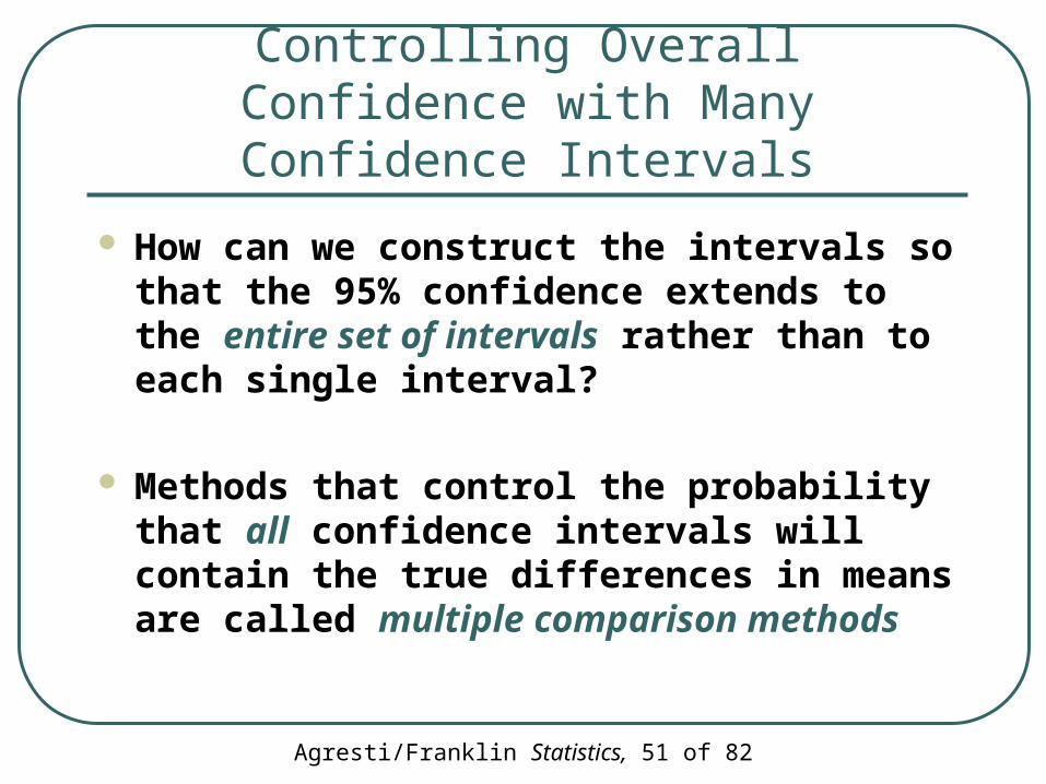
How can we construct the intervals so that the 95% confidence extends to the entire set of intervals rather than to each single interval?
Methods that control the probability that all confidence intervals will contain the true differences in means are called multiple comparison methods
Agresti/Franklin Statistics, 52 of 82
Controlling Overall Confidence with Many Confidence Intervals
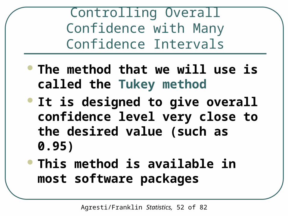
The method that we will use is called the Tukey method
It is designed to give overall confidence level very close to the desired value (such as 0.95)
This method is available in most software packages
Agresti/Franklin Statistics, 53 of 82
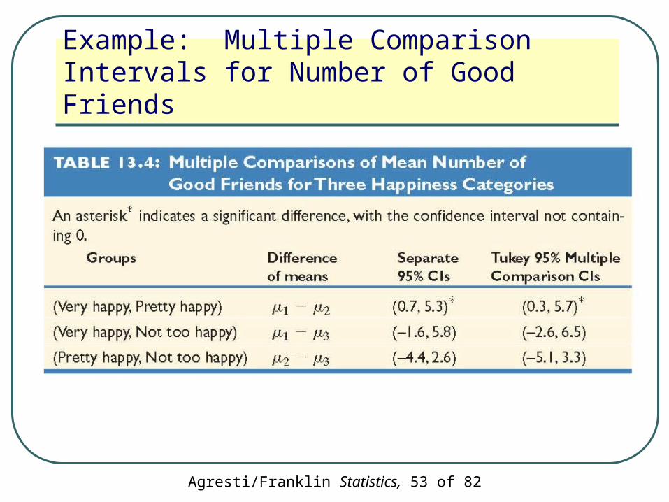
Example: Multiple Comparison Intervals for Number of Good Friends

Agresti/Franklin Statistics, 54 of 82
Section 13.3
What if There Are Two Factors?
Two-Way ANOVA
Agresti/Franklin Statistics, 55 of 82
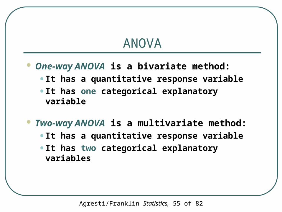
ANOVA
One-way ANOVA is a bivariate method:
• It has a quantitative response variable
• It has one categorical explanatory variable
Two-way ANOVA is a multivariate method:
• It has a quantitative response variable
• It has two categorical explanatory variables
Agresti/Franklin Statistics, 56 of 82
Example: How Does Corn Yield Depend on Amounts of Fertilizer and Manure?
A recent study at Iowa State University:
• A field was portioned into 20 equal-size plots
• Each plot was planted with the same amount of corn seed
• The goal was to study how the yield of corn later harvested depended on the levels of use of nitrogen-based fertilizer and manure
• Each factor (fertilizer and manure) was measured in a binary manner
Agresti/Franklin Statistics, 57 of 82
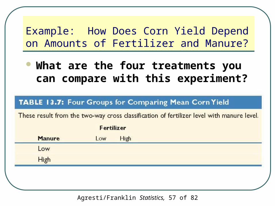
What are the four treatments you can compare with this experiment?
Example: How Does Corn Yield Depend on Amounts of Fertilizer and Manure?
Agresti/Franklin Statistics, 58 of 82
Inference about Effects in Two-Way ANOVA
In two-way ANOVA, a null hypothesis states that the population means are the same in each category of one factor, at each fixed level of the other factor
Agresti/Franklin Statistics, 59 of 82
We could test:
H0: Mean corn yield is equal for plots at the low and high levels of fertilizer, for each fixed level of manure
Example: How Does Corn Yield Depend on Amounts of Fertilizer and Manure?
Agresti/Franklin Statistics, 60 of 82
We could also test:
H0: Mean corn yield is equal for plots at the low and high levels of manure, for each fixed level of fertilizer
Example: How Does Corn Yield Depend on Amounts of Fertilizer and Manure?
Agresti/Franklin Statistics, 61 of 82
The effect of individual factors tested with the two null hypotheses (the previous two pages) are called main effects
Example: How Does Corn Yield Depend on Amounts of Fertilizer and Manure?
Agresti/Franklin Statistics, 62 of 82
Assumptions for the Two-way ANOVA F-test
1. The population distribution for each group is normal
2. The population standard deviations are identical
3. The data result from a random sample or randomized experiment
Agresti/Franklin Statistics, 63 of 82
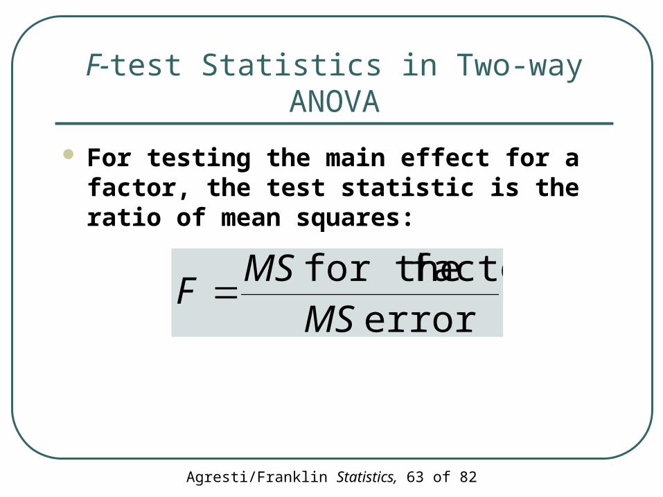
F-test Statistics in Two-way ANOVA
For testing the main effect for a factor, the test statistic is the ratio of mean squares:
error
factor for the
MS
MSF
Agresti/Franklin Statistics, 64 of 82
F-test Statistics in Two-way ANOVA
When the null hypothesis of equal population means for the factor is true, the F-test statistic values tend to fluctuate around 1
When it is false, they tend to be larger
The P-value is the right-tail probability above the observed F-value
Agresti/Franklin Statistics, 65 of 82
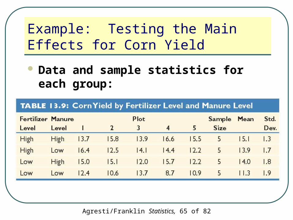
Example: Testing the Main Effects for Corn Yield
Data and sample statistics for each group:

Agresti/Franklin Statistics, 66 of 82
Example: Testing the Main Effects for Corn Yield
Output from Two-way ANOVA:
Agresti/Franklin Statistics, 67 of 82
Example: Testing the Main Effects for Corn Yield
First consider the hypothesis:
H0: Mean corn yield is equal for plots at the low and high levels of fertilizer, for each fixed level of manure
Agresti/Franklin Statistics, 68 of 82
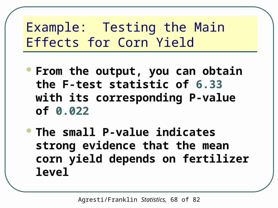
Example: Testing the Main Effects for Corn Yield
From the output, you can obtain the F-test statistic of 6.33 with its corresponding P-value of 0.022
The small P-value indicates strong evidence that the mean corn yield depends on fertilizer level
Agresti/Franklin Statistics, 69 of 82
Example: Testing the Main Effects for Corn Yield
Next consider the hypothesis:
H0: Mean corn yield is equal for plots at the low and high levels of manure, for each fixed level of fertilizer
Agresti/Franklin Statistics, 70 of 82
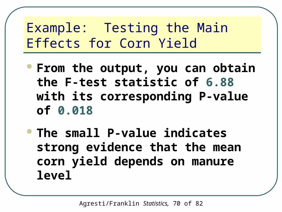
Example: Testing the Main Effects for Corn Yield
From the output, you can obtain the F-test statistic of 6.88 with its corresponding P-value of 0.018
The small P-value indicates strong evidence that the mean corn yield depends on manure level

Agresti/Franklin Statistics, 71 of 82
Exploring Interaction between Factors in Two-Way ANOVA
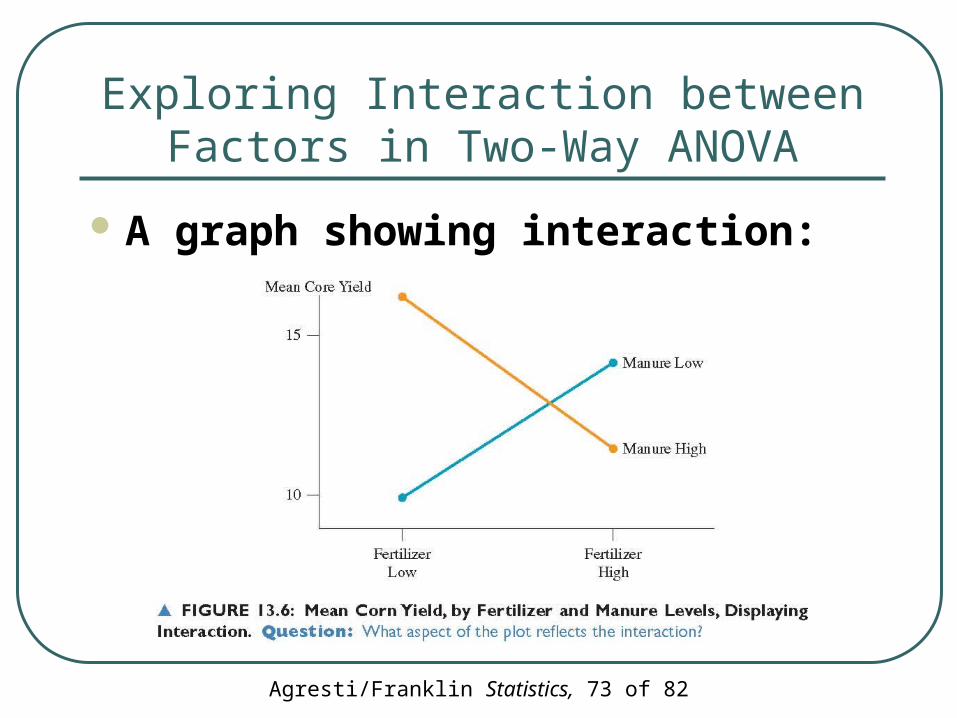
No interaction between two factors means that the effect of either factor on the response variable is the same at each category of the other factor

Agresti/Franklin Statistics, 72 of 82
Exploring Interaction between Factors in Two-Way ANOVA
Agresti/Franklin Statistics, 73 of 82
Exploring Interaction between Factors in Two-Way ANOVA
A graph showing interaction:

Agresti/Franklin Statistics, 74 of 82
Testing for Interaction
In conducting a two-way ANOVA, before testing the main effects, it is customary to test a third null hypothesis stating that their is no interaction between the factors in their effects on the response
Agresti/Franklin Statistics, 75 of 82
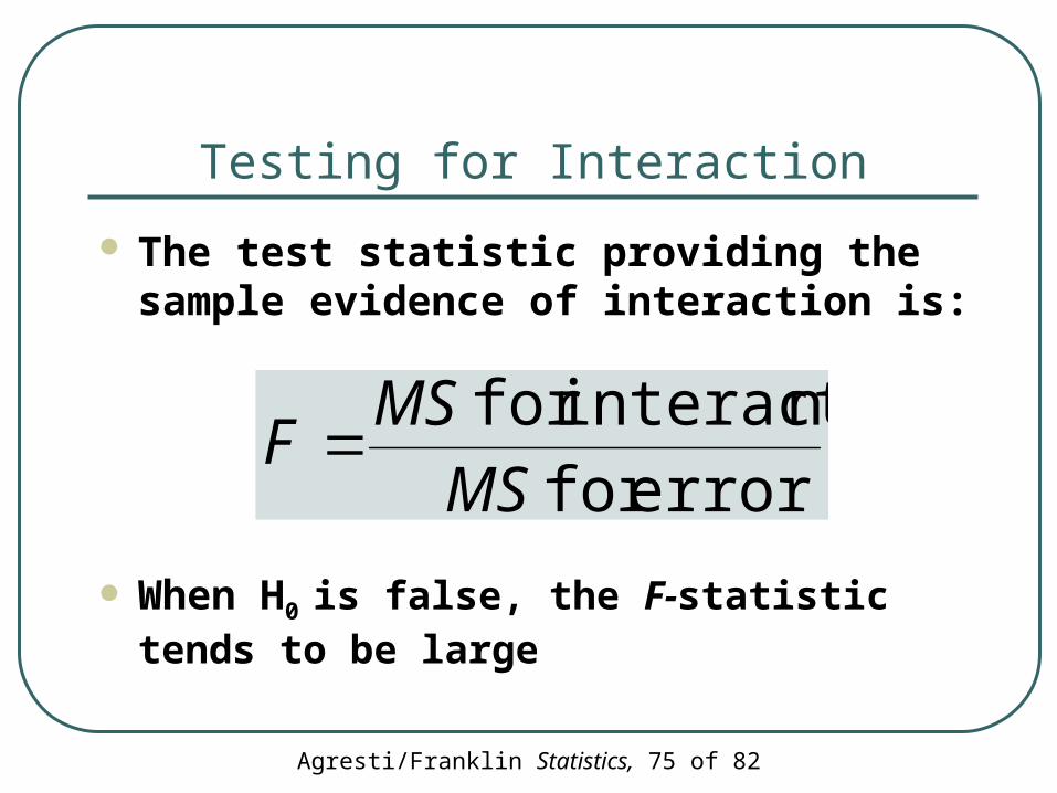
Testing for Interaction
The test statistic providing the sample evidence of interaction is:
When H0 is false, the F-statistic tends to be large
errorfor
ninteractiofor
MS
MSF
Agresti/Franklin Statistics, 76 of 82
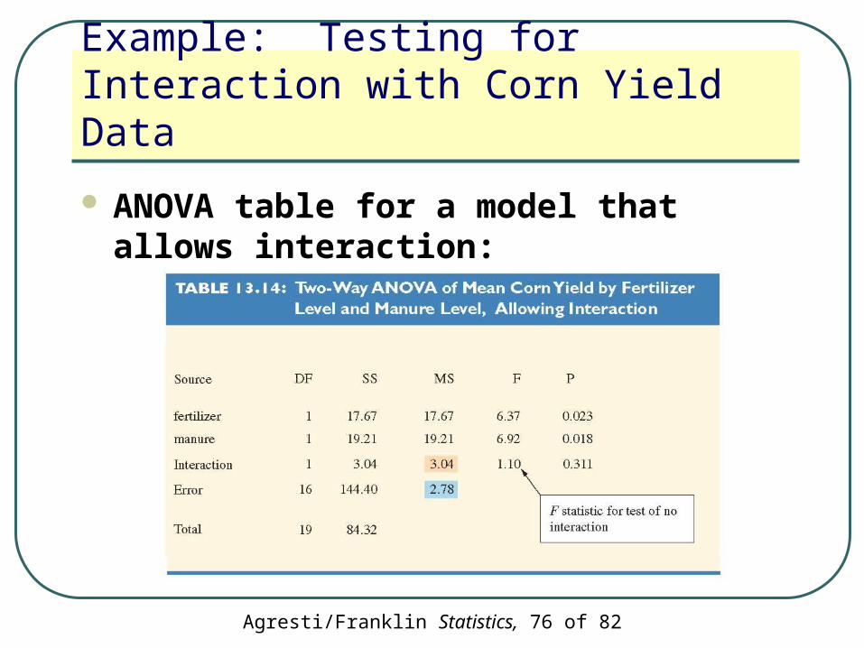
Example: Testing for Interaction with Corn Yield Data
ANOVA table for a model that allows interaction:
Agresti/Franklin Statistics, 77 of 82
Example: Testing for Interaction with Corn Yield Data
The test statistic for H0: no interaction is• F = 1.10 with a corresponding P-value
• of 0.311• There is not much evidence of
interaction• We would not reject H0 at the usual
significance levels, such as 0.05

Agresti/Franklin Statistics, 78 of 82
Check Interaction before Main Effects
In practice, in two-way ANOVA, you should first test the hypothesis of no interaction
Agresti/Franklin Statistics, 79 of 82
Check Interaction before Main Effects
If the evidence of interaction is not strong (that is, if the P-value is not small), then test the main effects hypotheses and/or construct confidence intervals for those effects
Agresti/Franklin Statistics, 80 of 82
Check Interaction before Main Effects
If important evidence of interaction exists, plot and compare the cell means for a factor separately at each category of the other factor
Agresti/Franklin Statistics, 81 of 82
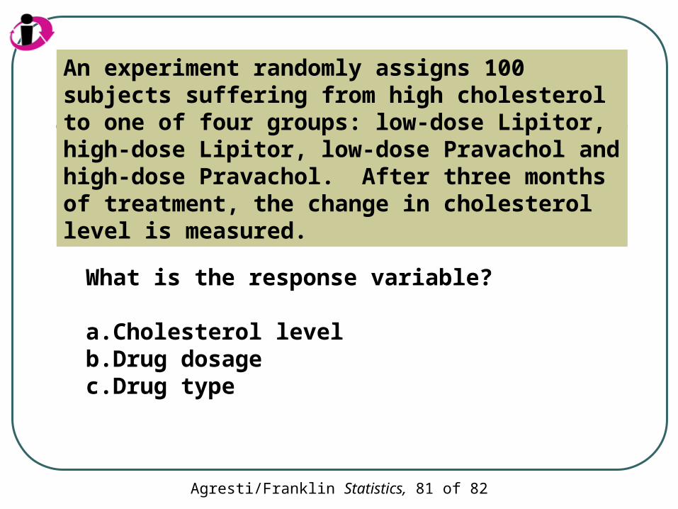
An experiment randomly assigns 100 subjects suffering from high cholesterol to one of four groups: low-dose Lipitor, high-dose Lipitor, low-dose Pravachol and high-dose Pravachol. After three months of treatment, the change in cholesterol level is measured.
What is the response variable?
a. Cholesterol levelb. Drug dosagec. Drug type
Agresti/Franklin Statistics, 82 of 82
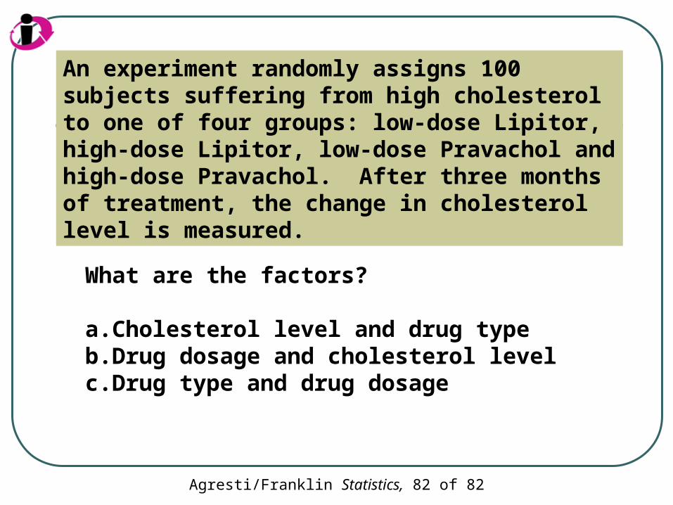
An experiment randomly assigns 100 subjects suffering from high cholesterol to one of four groups: low-dose Lipitor, high-dose Lipitor, low-dose Pravachol and high-dose Pravachol. After three months of treatment, the change in cholesterol level is measured.
What are the factors?
a. Cholesterol level and drug typeb. Drug dosage and cholesterol levelc. Drug type and drug dosage