agricultural activity and emissions projections to 2050 · web viewtotal milk production in...
TRANSCRIPT

www.TheCIE.com.au

2 Agricultural activity and emissions projections to 2050
R E P O RT
Agricultural activity and emissions projections to 2050
Prepared forDepartment of Environment14 April 2015
THE CENTRE FOR INTERNATIONAL ECONOMICSwww.TheCIE.com.auwww.TheCIE.com.au

The Centre for International Economics is a private economic research agency that provides professional, independent and timely analysis of international and domestic events and policies.The CIE’s professional staff arrange, undertake and publish commissioned economic research and analysis for industry, corporations, governments, international agencies and individuals.
© Centre for International Economics 2016This work is copyright. Individuals, agencies and corporations wishing to reproduce this material should contact the Centre for International Economics at one of the following addresses.
C A N B E R R ACentre for International EconomicsGround Floor, 11 Lancaster PlaceCanberra Airport ACT 2609GPO Box 2203Canberra ACT Australia 2601Telephone +61 2 6245 7800Facsimile +61 2 6245 7888Email [email protected] www.TheCIE.com.au
S Y D N E YCentre for International EconomicsSuite 1, Level 16, 1 York StreetSydney NSW 2000GPO Box 397Sydney NSW Australia 2001Telephone +61 2 9250 0800Facsimile +61 2 9250 0888Email [email protected] www.TheCIE.com.au
DISCLAIMER
www.TheCIE.com.au

While the CIE endeavours to provide reliable analysis and believes the material it presents is accurate, it will not be liable for any party acting on such information.

Agricultural activity and emissions projections to 2050 v
Contents
Summary 1Australia’s agricultural emissions 1Drivers of Australian agricultural production growth 1Meat production and animal numbers 2Dairy production and dairy cattle numbers 4Grain production 4Sensitivity analysis 5
1 Introduction 7This report 7Core projections methodology 7The models 8
2 Agricultural activity and emissions 10Key drivers of agricultural activity 10
3 Agricultural activity projections: model results 15Beef 15Sheep meat 20Pig meat 23Poultry 26Dairy industry 28Grain industries 31Other crops 35Fertiliser use 40Land constraint 43
4 Projected agricultural emissions 47Emissions projections in the context of history 47The broad composition of agricultural emissions 47Overview of emissions by sector and subsector 49Livestock related emissions 51Agricultural soils 53Crop emissions 53
5 Sensitivity analysis 55Variables for sensitivity analysis 55Sensitivity analysis results 56
www.TheCIE.com.au

vi Agricultural activity and emissions projections to 2050
References 73A Modelling approach 75B Baseline scenario assumptions 86
BOXES, CHARTS AND TABLES1 Agricultural emissions by broad sector 1990 to 2050 12 Australian meat production, 2013 and 2050 23 Australian animal numbers, 1990-2050 34 Australian dairy production growth by markets and dairy cattle
numbers 45 Australian grain production, 2013 and 2050 56 Variables tested with sensitivity analyses 57 Combined impact of sensitivity analysis on annual emissions 62.1 Drivers of agricultural emissions 102.2 Assumed world population growth 122.3 Average rate of assumed global economic growth 133.1 Beef and veal production and use projections 173.2 Projected beef production and exports: the baseline case 173.3 Projected beef cattle numbers: the baseline case 183.4 Comparison of beef cattle projections 203.5 Projected sheep meat production and exports: the baseline case 213.6 Sheep meat production and use projections 223.7 Projected sheep numbers: the baseline case 233.8 Comparison of sheep number projections 233.9 Projected pork production and exports: the baseline case 243.10 Pork production and use projections 253.11 Projected pig numbers: the baseline case 253.12 Comparison of pig number projections 263.13 Projected poultry meat production and exports: the baseline
case 274.14 Poultry meat production and use projections 273.15 Projected poultry numbers: the baseline case 273.16 Comparison of poultry number projections 283.17 Projected milk production by state: the baseline case 293.18 Projected use of Australian milk, index of quantity: baseline case 293.19 Projected dairy cattle numbers by state: the baseline case 303.20 Comparison of dairy cattle number projections 313.21 Projected grain production: the baseline case 323.22 Comparison of projected wheat production 343.23 Comparison of projected barley production 34
www.TheCIE.com.au

Agricultural activity and emissions projections to 2050 vii
3.24 Comparison of projected production of other coarse grains, million tonnes 35
3.25 Rice cultivation area and yield 363.26 Rice production 373.27 Sugarcane cultivation area and cane yield 383.28 Sugarcane crushed 393.29 Cotton area 393.30 Projected fertiliser use – the baseline case 413.31 Comparison of projected nitrogen fertiliser use, kt 423.32 Historical and projected use of fertilisers 423.33 Projected increase in cropping area 433.34 Total dry sheep equivalent of animals 443.35 Increase in cropping area and accumulated first conversion
area: historical versus projection 453.36 Land clearing areas 463.37 Total area of farms and cropping area 464.1 Total agricultural emissions (excluding prescribed burning of
savannas): 1990 to 2050 474.2 Emissions by broad sector 1990 to 2050 484.3 Emissions by broad sector 494.4 Agricultural emissions by sector and subsector 504.5 Livestock emissions 514.6 Enteric fermentation 524.7 Manure management 524.8 Agricultural soils 534.9 Crop emissions 544.10 Field burning of agricultural residues 545.1 Individual sensitivity analyses 555.2 Impact on emissions – percentage deviation from the central
reference case 565.3 Impact of foreign income sensitivity on annual emissions 585.4 Impact of foreign income on agricultural output 595.5 Impact of the exchange rate sensitivity on annual emissions 605.6 Impact of exchange rates on agricultural output 615.7 Impact of the productivity sensitivity on annual emissions 625.8 Impact of productivity on agricultural output 635.9 Growth rate in beef slaughter weights, historical and assumed
future rates 645.10 Impact of the slaughtering weight/yield sensitivity on annual
emissions 655.11 Impact of slaughtering weight and yield on agricultural output 665.12 Impact of the input price sensitivity on annual emissions 67
www.TheCIE.com.au

viii Agricultural activity and emissions projections to 2050
5.13 Impact of input prices on agricultural output 685.14 Impact of the lower supply response sensitivity on annual
emissions 695.15 Impact of lower supply responsiveness on agricultural output 705.16 Combined impact of sensitivity analysis on annual emissions 715.17 Combined sensitivity analysis result 72A.1 Sectors identified in CGE models 77A.2 Country groups and commodities identified in GMI 79A.3 Countries and regions in Dairy and Grains models 80A.4 Model parameters and their functions 83A.5 Range of income elasticities in the GMI model 84A.6 Range of price elasticities in the GMI model 84A.7 Elasticities for dairy products 84A.8 Demand elasticities for grain products 84A.9 Elasticities of transformation or substitution in the Grains model 85B.1 Trend historical growth for major global economies 86B.2 Average rate of assumed global economic growth 87B.3 Assumed price indexes of major fuel commodities 88B.4 Assumed world population growth 89B.5 Assumed Australian population growth 89B.6 Mining slowdown and agriculture 91B.7 Average slaughtering weight 92B.8 The ratio of slaughtered to animal numbers 92B.9 Assumed growth in slaughtering weight: GMI model 93B.10Assumed growth in the ratio of slaughtered to animal numbers:
GMI model 93B.11Long term productivity growth for meat commodities 95B.12Milk yield per cow and ratio of cow number to cattle number 96B.13Productivity improvement growth rate assumptions: the Dairy
model 96
www.TheCIE.com.au
Agricultural activity and emissions projections to 2050 1
Chart reports historical and projected greenhouse gas emissions from the Australian agricultural sector (excluding prescribed burning of savannas) from 1990 to 2050.
00Error! No text of specified style in document.A001 Agricultural emissions by broad sector 1990 to 2050
0
20
40
60
80
100
120
1990 1995 2000 2005 2010 2015 2020 2025 2030 2035 2040 2045 2050
Mt CO
2-e
Enteric Fermentation Manure ManagementRice Cultivation Agricultural SoilsField burning of agricultural residues Lime and Urea
Chart shows that enteric fermentation from livestock remains the largest component of total agricultural emissions through to 2050, accounting for over 70 per cent of emissions over the projection period.
Charts and summarise projected meat production and animal numbers arising from the projections.
www.TheCIE.com.au

2 Agricultural activity and emissions projections to 2050
00Error! No text of specified style in document.A002 Australian meat production, 2013 and 2050
Data source: CIE GMI modelling
00Error! No text of specified style in document.A003 Australian animal numbers, 1990-2050
05
101520253035
1990 2000 2010 2020 2030 2040 2050
Beef cattle
020406080
100120140160180200
1990 2000 2010 2020 2030 2040 2050
Sheep
0.00.51.01.52.02.53.03.5
1990 2000 2010 2020 2030 2040 2050
Pigs
020406080
100120140160180
1990 2000 2010 2020 2030 2040 2050
Poultry
Data source: DoE, CIE GMI modelling
Beef is the dominant meat product with over two thirds of production is for export. This high export share is expected to continue. Beef production is
www.TheCIE.com.au

Agricultural activity and emissions projections to 2050 3
projected to increase by 50 per cent over the projection period to meet increasing domestic and overseas demand, enabled by ongoing productivity growth in the sector. The number of beef cattle is projected to increase from 26 million in 2013 to about 32 million in 2050. This represents a growth rate of 0.5 per cent a year, on a par with historical growth.The situation for sheep meat is similar to beef. Over two thirds of sheep meat production in Australia is for export, and about 88 per cent of the projected increase in production from 2013 to 2050 is due to increased exports. It is projected that sheep numbers will increase by 9.3 per cent from 76 million in 2013 to 83 million in 2050 which is less than half the number in 1990.In contrast, the pig and poultry industries are domestically focused. Projected growth in pork production is mainly from growth in domestic fresh pork consumption that, due to quarantine restrictions, cannot be supplied from imports. It is projected that the number of pigs will increase by 34.3 per cent from 2.1 million in 2013 to 2.8 million in 2050.Compared to other meats, poultry is relatively cheap and demand for Australian poultry meat is projected to grow rapidly from 2013 to 2050. Around 40 per cent of the increase in poultry meat production is expected to come from export demand. Poultry numbers are projected to grow by 1.1 per cent a year from 2013 to 2050 to reach 154 million in 2050.
Dairy production and dairy cattle numbersTotal milk production in Australia is projected to increase by about 76 per cent to 16 170 million litres in 2050. This represents an annual growth rate of 1.5 per cent. Most of the increase in production is due to increases in export demand, driven by increasing population and incomes in developing economies. As shown by the left panel in chart , domestic demand is projected to grow by less than 1 per cent a year, while the exports of dairy products grow by more than 3 per cent a year. Because of assumed continued yield growth, the number of dairy cattle is projected to grow at a lower rate than milk production, 0.3 per cent per year, to 3.2 million in 2050 (right panel of chart ). This sees the number of dairy cattle recover to the historical record level observed in around 2000.
www.TheCIE.com.au

4 Agricultural activity and emissions projections to 2050
00Error! No text of specified style in document.A004 Australian dairy production growth by markets and dairy cattle numbers
0
1
2
3
4
5
6
7
8
Fresh UHT Manufactured Total dairy
% pa
Domestic Exports
2.0
2.2
2.4
2.6
2.8
3.0
3.2
3.4
1990 2000 2010 2020 2030 2040 2050m
illion
Data source: CIE Dairy model
Grain productionWheat production in 2050 is projected to be 90 per cent higher than it in 2013, while coarse grain production will increase by 74 per cent over the same period. As shown in chart , over 80 per cent of the increase in grain production is due to increasing export demand, driven by assumed population growth.
00Error! No text of specified style in document.A005 Australian grain production, 2013 and 2050
Data source: DoE, CIE Dairy model
www.TheCIE.com.au

Agricultural activity and emissions projections to 2050 5
Sensitivity analysisThe simulated outcomes from the economic models used as the basis for the emissions projections depend on a variety of ‘exogenous’ (or ‘outside’) input assumptions. The assumptions used are plausible future outcomes, partly based on historical observations, but the future values are not known with certainty.To gain some understanding of the extent that this uncertainty affects the results, sensitivity analysis is conducted for several key variables affecting agricultural production and emissions. The assumptions varied in the sensitivity analysis are summarised in table . Each of these are investigated separately as well as being combined to establish upper and lower bounds for emissions projections.
002B006 Variables tested with sensitivity analysesForeign income Input costs
Exchange rate Lower supply responsiveness
Productivity Slaughtering weight/yield
Of the range of variables tested, altering the supply responsiveness and exchange rate assumptions lead to the greatest change in total emissions, followed by productivity and slaughtering weight/yield assumptions.The combination of sensitivities suggests that in 2020, emissions could vary by 15-17 per cent around the central reference case. By 2050 the variation could be around 32 to 36 per cent. Most of the assumptions used indicate that agricultural emissions are expected to increase over time. These sensitivity results however show that, with alternative assumptions, emission levels projected for 2050 may be the same as, or even lower than, current agricultural emission levels.Thus, under the combined low case scenario, emissions could remain unchanged, or even decline from current levels over the forecast period.
www.TheCIE.com.au

6 Agricultural activity and emissions projections to 2050
005A007 Combined impact of sensitivity analysis on annual emissions
Note: The high and low under the combined scenario refer to the high and low emissions.Data source: CIE Grains, Dairy and GMI simulations
www.TheCIE.com.au

Agricultural activity and emissions projections to 2050 7
2 Introduction
This reportThis report provides projections of agricultural emissions to 20502. The report is structured as follows.■ The remainder of this introduction sets out key features of the
projections approach and methodology.■ Chapter 2 describes the key drivers of agricultural production and
emissions as a basis for understanding the projections.■ Chapter 3 sets out in detail the activity projections developed using the
core economic models.■ Chapter 4 presents the projected emissions, by sector and subsector,
based on the activity level projections.■ Chapter 5 sets out the results of sensitivity analysis around some of the
key assumptions underlying the central projections.■ Appendix A summarises the key features of the models used in the
analysis.■ Appendix B provides details of the input assumptions to those models.■ Appendix C provides additional information around the sensitivity
analysis.
Core projections methodology
Emissions coverageThis report covers six broad components of agricultural emissions:■ Enteric fermentation■ Manure management■ Rice cultivation ■ Agricultural soils ■ Field burning of agricultural residues
2 Emissions are projected for each year between 2013 and 2050. All the years mentioned in this report are financial years ending 30 June of that year.
www.TheCIE.com.au

8 Agricultural activity and emissions projections to 2050
■ Lime and urea.Projections presented here do not include prescribed burning of savannah and do not cover emissions from the Land Use, Land Use Change and Forestry (LULUCF) sector. Within this report, ‘total agricultural emissions’ refers to the sum of the above emissions categories.
Overall methodologyThe methodology for providing the emissions projections presented here contains two main elements.■ First, a number of economic models (see below) are used to project
‘activity levels’ for the agricultural activities that involve the generation of greenhouse gas emissions. These projections are produced at a highly disaggregated level and include livestock numbers, crop production, fertiliser use and so on.
■ Second, these activity levels are an input to a detailed emissions calculation spreadsheet developed by the Department of Environment (DoE). This spreadsheet converts activity levels to emissions projections for each of the emission sectors and subsectors.
Conformance with ABARES short term projectionsIn line with established practice and consistent with the longer term nature of the CIE models, we have used ABARES publications as a basis for short term projections to 2019. In particular Agricultural Commodities September Quarter 2014 (which includes the most recent update to projections to 2015) and Agricultural Commodities March Quarter 2014 (includes projections to 2019) are used.
Central reference and sensitivity analysesThe main set of emissions projections are around a ‘central reference case’, which essentially involves a business as usual set of projections for the agricultural sector. Note that the central reference case does not account for drought or other stochastic climatic influences on agricultural output. This is important to keep in mind when interpreting the longer-term projections relative to recent history.The analysis includes sensitivity analysis around a number of key exogenous modelling assumptions — reflecting the fact that there is inevitable uncertainty around some of these assumptions.
www.TheCIE.com.au

Agricultural activity and emissions projections to 2050 9
The models
Key modelsThe central reference case projections and the sensitivity analyses are developed using a suite of agricultural commodity models developed and maintained by the CIE. These models are:■ The Global Meat Industry (GMI) model of 10 meat products in 23
countries and regions;■ The Dairy model of the production and use of milk and dairy products in
Australian states and territories as well as in Australia’s key competitor countries/regions; and
■ The Grains model of wheat, barley, oilseeds, pulses and other coarse grain production and consumption in Australian states and territories as well as in Australia’s key markets and competitors.
In addition, spreadsheet models are used as supplementary tools for some agricultural products not formally included in the above models, including rice, cotton and sugarcane. General equilibrium models of the global and Australian economies (CIE G-Cubed and CIE Regions) are used to project external demand, production and prices and used as inputs to the commodity models. Further details on the models used are provided in Appendix A.
Input assumptionsDeveloping the projections with these economic models requires assumptions about a number of key model drivers. Details of these assumptions are set out in Appendix B. These assumptions are all based on plausible future outcomes within the agricultural sector and the wider economy.While the central reference case has input assumptions based partly on history (which includes the average effects of drought) it does not incorporate assumptions based on extreme values. Thus, the future is an average expectation that does not account for the possibilities of extreme events.
www.TheCIE.com.au

10 Agricultural activity and emissions projections to 2050
3 Agricultural activity and emissions
Agricultural emissions are determined by the level of agricultural activities, which are, in turn, determined by a set of demand and supply side factors. This chapter discusses these factors in the context of history and explains how they affect the activity and emissions.
Key drivers of agricultural activityEmissions from the agriculture sector are primarily driven by the level of agricultural activity undertaken. The activity levels, in turn, are influenced by a range of factors to which agricultural producers react and respond. Farmers observe changes in demand and market conditions through the prices they receive for their products.
www.TheCIE.com.au

Agricultural activity and emissions projections to 2050 11
022A028 Drivers of agricultural emissions
Data source: The CIE
Chart sets out the key factors that affect agricultural activity levels, and therefore emissions. While every factor can affect each activity, the extent of the influence on activity levels differs between depending on the nature of products and markets. Seasonal conditions, increasing demand driven by increases in incomes and population, and changes in broad economic markets significantly affect all Australian agricultural production and are described below.
Seasonal conditionsWeather, or seasonal conditions, is the principal driver of change in Australian agricultural production. Although the precise ways in which weather affects each industry differs, and weather conditions vary spatially across the country, weather has significant effects on Australian agricultural production by physically constraining possible production levels (for example, reducing the number of livestock that can be maintained in times of poor pasture, or reducing the possible volume of crop production where there is limited water available).It is hard, if not impossible, to predict changes in seasonal conditions. Changes in seasonal conditions are only incorporated into the short term
www.TheCIE.com.au
Emissionsenteric fermenation; manure management; rice cultivation; agricultural soils; field
burning of agricultural residues; lime and urea
Activity levelsnumber of animals; area cropped; crop production; fertiliser applied, lime and
urea use
Supply side
Productivity/Yields
Seasonal
conditions
Resource
constraints
Farm gate prices
Demand side factors
Domestic demand
Population
Incomes
Preferences
International demand
Population
Incomes
Preferences
Market conditions
Export
competitio
n
Trade barrie
rsExchange
rates
Emissio
n factors

12 Agricultural activity and emissions projections to 2050
projections by assuming conditions return to average in 2015. Between 2015 and 2019 some livestock sectors, which have longer adjustment periods than crops, see production changes as a result of this return to average seasonal conditions. In the longer term (beyond 2019) seasonal conditions are assumed to remain average. Sensitivity analysis (the ‘lower supply responsiveness’ scenario) in chapter 5 explores the potential impact of changes to this assumption.
Resource constraintsAgricultural producers are also affected by the availability of land and labour. Demand for these resources from other, higher return activities, affects the productivity and activity levels in agricultural industries. Continued development of agricultural land for residential and mining activities has been forcing agricultural production onto less productive land, reducing potential yield growth. In some cases this has led farmers to increase the use of fertilisers and therefore to increase emissions. In the past decade, demand for labour from the mining sector drove an increase in the cost of labour across the economy. Generally higher labour costs affects producers across the agricultural sector – increasing the cost of production. As the growth in the mining sector slows, the growth rate of labour costs is expected to decline.
Productivity and yieldsAgricultural productivity has continually increased in the past, and is particularly reflected in increased yields. Improvements in agricultural productivity tend to lead to an increase in production. By lowering the marginal cost of production, productivity improvements mean that for any given price, producers find it profitable to produce more.Productivity improvements in the agricultural sector have been realised through improved equipment, technology developments, improved genetics and general efficiency gains. Research, development and deployment of new technologies and techniques, for example genetic modification, is expected to continue and this is incorporated into the activity projections by assuming continued productivity growth. Details of the assumed productivity growth for each of the agricultural industries are outlined in Appendix B. Compared to the 2013 projections, assumed productivity growth rates in this report are lower, leading to slower growth in production over the projection period compared to the 2013 projections3.
3 Slower assumed productivity growth rates are based on discussions with industry exports.
www.TheCIE.com.au

Agricultural activity and emissions projections to 2050 13
Demand side factorsPopulation and income growth overseas will ensure there is growing demand for Australian agricultural products. With increasing population and incomes, particularly in key export markets, our models suggest agricultural output will also increase.Strong population growth is projected for the period to 2050, especially in Asia and other developing economies (see chart ).
022A029 Assumed world population growth
Data source: UN Population Division, ABS
Economic growth is also projected to be strong, reflecting continued development in developing economies and recovery from the global financial crisis (GFC). Again, growth rates in Asia and other developing countries are particularly strong, especially early in the projection period. Increasing incomes are expected to drive increased demand for all products, but higher protein foods such as meat and dairy products in particular.
Comparison with 2013 projections
The global economic growth assumptions used in this projection are lower than those used in the 2013 projections. This is due to slower than expected recovery from the GFC. As economic growth is a key driver of global demand for agricultural products, the lower assumed growth rate is reflected in all the activity level projections with slower growth in production over the projection period.
www.TheCIE.com.au

14 Agricultural activity and emissions projections to 2050
022B0210 Average rate of assumed global economic growth2013-19 2020-25 2026-40 2041-50
%pa %pa %pa %pa
Australia 3.06 3.20 2.82 2.59China 7.05 6.22 5.41 4.56India 6.10 6.44 5.57 4.67US 2.62 2.23 2.27 2.32European Union 1.52 1.86 1.95 2.06Rest of Asia 2.83 3.02 2.94 2.83Rest of the World 3.08 3.47 3.30 3.10Source: IMF (2014a) for 2013-19; CIE assumptions for 2020-50
Market conditionsTrade barriers and exchange rates affect the price of Australian products therefore alters the demand and supply of Australian products.Trade barriers, such as tariffs, drive a wedge between the price consumers pay and producers receive. Removing that wedge through trade liberalisation lowers prices for consumers and increases prices for producers. Both tend to increase production. Australia has recently concluded negotiating free trade agreements with Japan and Korea.4 Gradual removal of trade barriers under these agreements will, all else equal, increase Australian production and exports. Similarly, a depreciation of the Australian dollar will increase Australian production. A lower Australian dollar means cheaper price in foreign currencies which are faced by foreign consumers, and thus encouraging more demand for Australian products. On the other hand, for goods priced in foreign currencies (which tends to be the case for some Australian agricultural exports), a lower Australian dollar means an increase in Australian farm gate prices and encourage an increase in Australian production. The Australian dollar experienced a rapid appreciation after the GFC, due to the safe nature of the dollar as well as high demand for Australian minerals. Exchange rate projections for the analysis were provided by DoE as set out in Appendix B.
4 The modelling for this report was undertaken before the announcement of the China-Australia Free Trade Agreement and therefore it isn’t considered as part of the analysis.
www.TheCIE.com.au

Agricultural activity and emissions projections to 2050 15
Australian producers are also negatively affected by trade agreements between other countries. For example, the trade agreement between New Zealand and China means that New Zealand products enter the Chinese market at lower prices than Australian products (from the point of view of Chinese consumers). Gradual tariff reductions mean the impact of these trade agreements will increase over the projection period.Biosecurity measures have proven to be one of the most significant factors affecting trade flows recently. Restrictions on the import of beef from the US to Japan and China due to BSE concerns meant Australian producers were able to secure significant market share in these high value markets. Relaxation of these restrictions is expected to lead to lower exports to these markets from Australia (although produce is expected to be redirected to other markets and therefore not significantly affect production levels).Box provides a description of how changes in the mining sector is affecting agriculture and provides a tangible example of some of the effects described above.
www.TheCIE.com.au

16 Agricultural activity and emissions projections to 2050
4 Agricultural activity projections: model results
Emissions projections are a combination of activity level forecasts (variables such as livestock numbers, crop production and fertiliser application) along with the emissions factors associated with those activity levels.
This chapter presents modelled activity level results in detail, working through the core outcomes and drivers of each of the economic models used for the projections analysis.
For the short term projections up to 2019, our modelling adopts commodity forecasts by ABARES which are based on accurate current information on micro factors such as farm gate prices, farm soil moisture and seasonal weather conditions, yield changes and animal dynamics. For the longer term, uncertainty about these factors is greater and projections are produced according to our assumptions about the future demographic and economic growth as well as the relationship underlying the demand for, and supply of, Australian agricultural commodities.
Beef
Beef meat productionMost of Australia’s production of beef is exported and therefore the international beef markets are a key driver of Australian beef production. International demand for beef is projected to continue to increase over the projection period on the back of strong population and economic growth (as explained in the previous chapter and outlined in Appendix B), particularly in China and other developing economies. In developing countries, beef is highly income ‘elastic’, so that increases in income lead to proportionate increases in beef demand. Another key demand factor is the free trade agreements with Japan and Korea, which are projected to change trade patterns. These agreements are a significant part of the continual increase in demand for Australian meat.
www.TheCIE.com.au

Agricultural activity and emissions projections to 2050 17
The modelling shows a projected increase in real prices for beef, an indicator that growth in global demand is faster than the rate of growth of supply. In this environment of strong international demand for beef and a rising world price, Australian beef production will be determined by domestic conditions that enable increased production – productivity improvements, seasonal conditions and resource constraints. The ability of farmers to increase production in response to higher prices is manifested in the price elasticity of supply which ranges from 0.4 to 0.6 for beef (see table in appendix A). This reflects constraints on the availability of factors of production such as land and labour. At the same time, assumed productivity growth of up to 0.75 per cent a year will mean Australian farmers are able to increase beef production for a given level of available inputs. For the grain fed beef sector, the cost of feed grain is also a consideration. Feed grain prices are projected to increase by around 0.4 per cent a year over the projection period which may dampen the expected increase in grain fed beef production.Current poor seasonal conditions have led to an increase in Australian cattle turn-off and meat production has risen accordingly (9.8 per cent increase from 2013 to 2014). As seasonal conditions are assumed to return to average from 2015, meat production is expected to decline initially as producers rebuild herds and lower the number of cattle slaughtered. Meat production is projected to increase again from 2018 (see chart ). Projected exports follow the same pattern. Global surplus demand for beef (as indicated by increasing real prices) means that changes in competition from other producers tend to lead to changes in destinations of Australian beef exports rather than a change in the volume produced and exported. In the short term to 2019, beef production in the US is projected to fall as seasonal conditions improve resulting in a decline in slaughter numbers and curtailing of herd liquidation. Beef exports from New Zealand (a major exporter to the US market) are also projected to be lower in the short term as seasonal conditions improve there too. Lower production from these countries means that Australian producers will sell more products to the higher value markets (Japan and Korea).On the other hand, international trade in beef has been significantly affected by BSE concerns in the recent past – with Japan and China both imposing restrictions on imports of beef from the US. These restrictions are being relaxed and US exports to these countries is projected to increase over the next few years, potentially displacing Australian production. Australian beef products will be re-directed to less valuable markets (and therefore lead to slightly lower prices for Australian producers than would be the case had restrictions on US imports remained).
www.TheCIE.com.au

18 Agricultural activity and emissions projections to 2050
In the longer term (after 2019), with seasonal conditions assumed to return to average and no significant changes in the costs of factors of production expected, Australia’s beef meat production is projected to increase as farmers respond to higher prices. Beef production in 2050 is projected to be 36.6 per cent higher than in 2014.Domestic demand for beef is projected to steadily increase in line with historical experience and projected growth in population and incomes. Because growth in Australian population and income is not as strong as in overseas markets, the significance of exports in total Australian production is projected to increase over the projection period (see chart )
033A0311 Beef and veal production and use projections
Data source: ABARES (2014) and CIE GMI modelling
033B0312 Projected beef production and exports: the baseline case2013 2014 2015 2019 2020 2030 2050 CAGR
kt kt kt kt kt kt kt %ProductionGrass fed 1572.7 1726.2 1667.4 1581.1 1615.9 1885.0 2435.4 1.2Grain fed 552.9 606.9 586.2 555.9 565.7 638.0 742.7 0.8Live 119.3 130.9 126.5 119.9 122.2 142.4 186.8 1.2ExportsGrass fed 1147.4 1340.4 1278.8 1180.8 1209.0 1416.9 1849.2 1.3Grain fed 219.0 255.8 244.0 198.2 202.6 226.7 211.6 -0.1Live 119.3 130.9 126.5 119.9 122.2 142.4 186.8 1.2Source: CIE GMI model simulation
www.TheCIE.com.au

Agricultural activity and emissions projections to 2050 19
Beef cattle numbersFor the beef industry, it is the number of cattle that determines emissions. In the GMI model this is in turn determined by three factors: the growth in demand for Australian meat products (which, as outlined
above, is largely driven by export demand, which in turn depends on population and income growth in our trading partners);
the slaughter weight of the animals concerned — a higher slaughter weight, for example, means that a given meat demand is associated with fewer head of stock; and
the ratio of the number of animals slaughtered to the total number of animals.
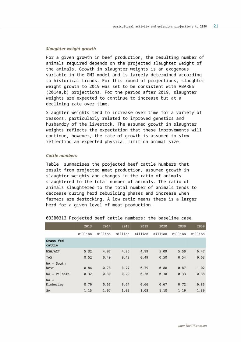
Slaughter weight growth
For a given growth in beef production, the resulting number of animals required depends on the projected slaughter weight of the animals. Growth in slaughter weights is an exogenous variable in the GMI model and is largely determined according to historical trends. For this round of projections, slaughter weight growth to 2019 was set to be consistent with ABARES (2014a,b) projections. For the period after 2019, slaughter weights are expected to continue to increase but at a declining rate over time.Slaughter weights tend to increase over time for a variety of reasons, particularly related to improved genetics and husbandry of the livestock. The assumed growth in slaughter weights reflects the expectation that these improvements will continue, however, the rate of growth is assumed to slow reflecting an expected physical limit on animal size.
www.TheCIE.com.au

20 Agricultural activity and emissions projections to 2050
Cattle numbers
Table summarises the projected beef cattle numbers that result from projected meat production, assumed growth in slaughter weights and changes in the ratio of animals slaughtered to the total number of animals. The ratio of animals slaughtered to the total number of animals tends to decrease during herd rebuilding phases and increase when farmers are destocking. A low ratio means there is a larger herd for a given level of meat production.
033B0313 Projected beef cattle numbers: the baseline case2013 2014 2015 2019 2020 2030 2050
million million million million million million millionGrass fed cattleNSW/ACT 5.32 4.97 4.86 4.99 5.09 5.50 6.47TAS 0.52 0.49 0.48 0.49 0.50 0.54 0.63WA - South West 0.84 0.78 0.77 0.79 0.80 0.87 1.02WA – Pilbara 0.32 0.30 0.29 0.30 0.30 0.33 0.38WA – Kimberley 0.70 0.65 0.64 0.66 0.67 0.72 0.85SA 1.15 1.07 1.05 1.08 1.10 1.19 1.39VIC 2.36 2.20 2.15 2.21 2.25 2.44 2.86QLD 11.89 11.09 10.86 11.15 11.36 12.29 14.45NT 2.20 2.05 2.01 2.06 2.10 2.27 2.67Total 25.29 23.60 23.10 23.71 24.16 26.15 30.73Grain fed cattleNSW/ACT 0.28 0.26 0.25 0.26 0.26 0.28 0.29TAS 0.00 0.00 0.00 0.00 0.00 0.00 0.00WA 0.03 0.03 0.03 0.03 0.03 0.03 0.03SA 0.05 0.04 0.04 0.04 0.04 0.05 0.05VIC 0.07 0.07 0.07 0.07 0.07 0.07 0.08QLD 0.74 0.69 0.67 0.69 0.70 0.74 0.78NT 0.00 0.00 0.00 0.00 0.00 0.00 0.00Total 1.16 1.09 1.06 1.09 1.11 1.16 1.23Source: CIE GMI model simulation
Grass fed cattle numbers are projected to fall initially from 25 million in 2013 to 24 million in 2019. After 2019, numbers are projected to gradually increase to 26 million by 2030 and to 31 million by 2050. This represents an average annual growth rate of 0.5 per cent between 2013 and 2050. These herd dynamics reflect increased slaughterings and lower calving rates in eastern Australia in 2014 in response to poor seasonal conditions that are unable to support large herds. Then, as conditions are assumed to return to average after 2015, herds are rebuilt with cattle numbers steadily increasing.
www.TheCIE.com.au

Agricultural activity and emissions projections to 2050 21
Grain fed cattle numbers follow a similar pattern. They are projected to fall from 1.16 million in 2013 to 1.09 million in 2019, before gradually rising to 1.16 million by 2030 and to 1.23 million by 2050. This represents an average annual growth rate of 0.14 per cent between 2013 and 2050.
Comparison with 2013 projectionsProjected beef production is lower than projected in the 2013 projection round. The differences between the current and 2013 projections are explained by three factors:■ a CIE assumption that long term productivity growth is lower than
previously assumed■ assumed lower economic growth rates compared to the 2013 projection■ a lower level of beef production projected for 2019 by ABARES
reflecting changes in seasonal condition, which is used as the starting point for CIE’s modelling.
Compared to the 2013 projections, this projection is based on an assumed lower level of productivity in Australia’s beef industry. More specifically, the current assumed productivity improvement is about three quarters of the improvement assumed in the last round of projections. This change reflects the view of industry experts.5■ Expectations of future production out of the northern cattle industry
have been revised down because of slowing growth of total factor productivity over the last decade and a combination of recent bad seasons and lower levels of profitability.
■ Throughout 2013, drought and the subsequent selloff of breeding stock from southern Queensland through to the Northern Territory resulted in lower herd numbers that will need to be rebuilt over the period to 2019 and thus the productivity of the sector will be lower than otherwise expected.
■ Further pressure on key costs such as the availability of hired labour, is likely to limit productivity improvements in the future as producers take a more conservative approach to stocking rates and input use.
Export growth is projected to be lower than in the 2013 projection because of the prolonged global economic downturn and relative weaker competiveness of Australian products due to the lower assumed productivity improvement in the industry. The short term projection of meat production (from 2014 to 2019) for this projection from ABARES (2014a,b) provides a lower base for our longer term projections compared to that used for the 2013 projections.
5 Industry views are gathered by the CIE through ongoing engagement with the meat industry.
www.TheCIE.com.au

22 Agricultural activity and emissions projections to 2050
According to ABARES (2014a,b), total beef production in Australia will be 2 257 kt in 2019. This is 5.2 per cent lower than the level used in the 2013 projection round. The lower projected beef production in 2019 reflects the poor seasonal conditions experienced in 2014 and subsequent need to rebuild herds and lower production in the short term to 2019.
033A0314 Comparison of beef cattle projections
20
25
30
35
40
45
1990 1995 2000 2005 2010 2015 2020 2025 2030 2035 2040 2045 2050
milli
on
2014 2013 ABARES 2014
Data source: DoE, ABARES (2014a,b) and CIE GMI modelling
Compared with the 2013 projection round, the current projections for cattle numbers are also lower in all years (chart ). This reflects lower growth in beef production (lower productivity growth), lower demand for beef (from lower economic growth levels) and a lower base level of cattle numbers.
Sheep meatAs is the case with beef production, strong and growing export markets (due to the assumed growth in overseas populations and incomes) ensure there is growing demand for sheep meat products and production is mostly affected by supply constraints within Australia. Key markets for sheep meat exports are the Middle East and China, both projected to have strong income growth over the projection period. In the case of China, economic growth is the main driver of demand as China’s population is assumed to increase by 5.5 per cent to 2030 but then decline back to 2012 levels by 2050. The economic growth rate for China on the other hand is assumed to average 5.6 per cent over the projection period. In the region including the Middle East, both the population growth rate (1.5 per cent) and the economic growth rate (3.2 per cent) are assumed to be high over the projection period.Australian production of sheep meat is mostly (68 per cent) exported. Declining domestic lamb consumption per person in response to continued
www.TheCIE.com.au
Agricultural activity and emissions projections to 2050 23
increasing prices is projected to be offset by increased exports, increasing the share of production that is exported to 71 per cent.Dry conditions in Australia have driven recent increased lamb offerings as farmers reduced animal numbers. From 2015 to 2019 production of sheep meat (total lamb and mutton production) is expected to decline as flocks are rebuilt assuming a return to average seasonal conditions. Total sheep meat production is projected to be 613kt in 2019, a 1.8 per cent fall from 2015. After 2019, production and exports of sheep meat are projected to increase in response to continued demand growth, currency depreciation and increasing real prices. An assumed productivity growth rate of 0.4 per cent a year for lamb will mean farmers are able to produce more lamb per unit of inputs each year, enabling continued increased production over the projection period.New Zealand is the only major competitor for Australian exports of sheep meat. New Zealand has a free trade agreement with China which is resulting in declining tariffs for New Zealand sheep meat exports to China. New Zealand also enjoys a tariff free quota for exports to the EU. These trade agreements mean that New Zealand sheep meat is likely to gain an increasing share of these markets, with Australian production exported to other markets, such as the Middle East.However, New Zealand exports of lamb are expected to fall in 2014 in response to drought in early 2013 that affected lambing rates. Continued competition for land with dairy farming is also contributing to expected lower production from New Zealand over the next few years, allowing Australian producers a greater share of the high value markets (all else equal).
033B0315 Projected sheep meat production and exports: the baseline case
2013 2014 2015 2019 2020 2030 2050 CAGR
kt kt kt kt kt kt kt %Production 640.2 702.2 624.4 613.3 620.9 673.5 774.7 0.5Sheep meat exports
404.8 479.3 407.0 386.4 392.4 431.3 520.2 0.7
Live export 86.4 94.7 84.2 82.7 83.8 92.7 112.7 0.7Source: CIE GMI model simulation
www.TheCIE.com.au

24 Agricultural activity and emissions projections to 2050
033A0316 Sheep meat production and use projections
Note: The chart on the left does not include live exports, whereas the chart of the right does – the two charts can therefore not be directly comparedData source: ABARES (2014) and CIE GMI modelling
Sheep numbersAs is the case with beef, the number of sheep determines emissions which is in turn determined by the demand for sheep meat, slaughter weight of the animals and the ratio of the number of animals slaughtered to the total number of animals. Sheep slaughter weights are assumed to grow over the projection period (see appendix B for details), leading to fewer sheep required for the given level of meat demand. The ratio of animals slaughtered to the total number of animals tends to decrease during herd rebuilding phases, as expected in the period from 2015 to 2019. Therefore, during this period a larger flock size is projected for a given level of meat productionSheep numbers are projected to fall in 2014 and 2015 to 71 million through increased slaughterings in response to dry conditions before starting to rise with gradual flock rebuilding starting in 2016, and reach 75 million in 2019, consistent with ABARES (2014a,b). Numbers are projected to further rise to 78 million in 2030 and 83 million in 2050 to meet the projected sheep meat production. The average annual growth rate between 2013 and 2050 is 0.2 per cent. Projected sheep numbers are summarised in table .
www.TheCIE.com.au

Agricultural activity and emissions projections to 2050 25
033B0317 Projected sheep numbers: the baseline case2013 2014 2015 2019 2020 2030 2050
million million million million million million millionSheepNSW/ACT 27.85 26.55 26.33 27.66 28.52 28.89 30.46TAS 2.40 2.29 2.27 2.38 2.46 2.49 2.62WA 15.47 14.74 14.62 15.36 15.84 16.04 16.91SA 10.82 10.31 10.23 10.74 11.08 11.22 11.83VIC 16.07 15.31 15.19 15.95 16.45 16.66 17.57QLD 2.94 2.80 2.78 2.92 3.01 3.05 3.21NT 0.00 0.00 0.00 0.00 0.00 0.00 0.00Total 75.55 72.01 71.41 75.01 77.36 78.36 82.60Source: CIE GMI model simulation
Comparison with 2013 projectionsCompared with the 2013 projections, the current projections of sheep numbers are lower – 18 per cent lower in 2050. This is due to lower base level – 9.7 per cent lower in 2019 – and a slower growth rate after that which reflects the slower growth rate in sheep meat demand, due to slower assumed world economic growth rates (see chapter 2) (chart ).
033A0318 Comparison of sheep number projections
50
70
90
110
130
150
170
190
1990 1995 2000 2005 2010 2015 2020 2025 2030 2035 2040 2045 2050
milli
on
2014 2013 ABARES 2014
Data source: ABARES (2014a,b), DoE, CIE GMI modelling
Pig meatAustralia is a net importer of pig meat, importing meat from the US, EU and Canada. Quarantine laws, however, restrict imports of pork to deboned products used in processed meat products. The Australian pork industry, therefore, primarily serves domestic demand for fresh pork
www.TheCIE.com.au

26 Agricultural activity and emissions projections to 2050
products. Domestic consumption of pig meat is projected to continue to rise over the projection period, driven by the assumed increasing population (1.3 per cent per year) and slower price growth compared to beef and lamb making pork a relatively cheaper alternative. Consumption of pork is projected to increase by 29 per cent over the projection period, or an average annual rate of 0.7 per cent. Australia is also a small exporter of pig meat. Australian exports of pig meat are expected to increase, particularly to Singapore and New Zealand, due to the assumed currency depreciation. Seasonal conditions have less impact on production levels compared to beef and lamb production because most pigs housed in enclosed buildings, they are protected from the weather and rely on feed rather than pastures. Seasonal conditions, however, still affect the sector indirectly through the price of feed grain. The price of feed grains are projected to increase by around 0.4 per cent a year over the projection period, a result of increasing demand across the intensive livestock sectors.Productivity growth in the pork industry is assumed to be 0.8 per cent a year which will enable increased pork production throughout the projection period, despite increased input costs. From 2020 to 2050, slaughter weight for pigs is projected to increase (growing at an average annual rate of 0.3 per cent), thereby reducing the number of pigs required to meet projected pork production. To achieve the projected pork production volumes, pig numbers are projected to gradually increase from 2.1 million in 2013 to 2.2 million in 2020, 2.4 million in 2030 and 2.8 million in 2050. The average annual growth rate is 0.8 per cent between 2013 and 2050. Table summarises projected pig numbers in selected years.
033B0319 Projected pork production and exports: the baseline case2013 2014 2015 2019 2020 2030 2050 CAGR
kt kt kt kt kt kt kt %Production 355.82 359.84 363.95 373.98 381.62 430.98 527.78 1.07Exports 26.23 26.77 28.09 30.66 32.72 48.85 102.43 3.75Source: CIE GMI model simulation
www.TheCIE.com.au

Agricultural activity and emissions projections to 2050 27
033A0320 Pork production and use projections
Data source: ABARES (2014) and CIE GMI modelling
033B0321 Projected pig numbers: the baseline case2013 2014 2015 2019 2020 2030 2050
million million million million million million millionPigsNSW/ACT 0.50 0.51 0.52 0.53 0.54 0.58 0.67TAS 0.01 0.01 0.01 0.01 0.01 0.01 0.01WA 0.22 0.23 0.23 0.23 0.24 0.26 0.30SA 0.31 0.32 0.32 0.33 0.33 0.36 0.42VIC 0.51 0.52 0.53 0.54 0.54 0.59 0.68QLD 0.55 0.56 0.56 0.57 0.58 0.63 0.73NT 0.00 0.00 0.00 0.00 0.00 0.00 0.00Total 2.10 2.15 2.17 2.21 2.25 2.44 2.82Source: CIE GMI model simulation
Comparison with 2013 projectionsCompared with the 2013 round of projections, the current projection of pig numbers is 21 per cent lower in 2050 (chart ). This is mainly due to the slower growth rate cumulated over the projection period, driven by slower assumed world economic growth (see chapter 2).
www.TheCIE.com.au

28 Agricultural activity and emissions projections to 2050
033A0322 Comparison of pig number projections
Data source: ABARES (2014a,b) and CIE GMI modelling
PoultryAustralia does not import chicken meat (due to quarantine restrictions), and has minimal chicken exports (because international demand is largely met by production in low cost countries). The production of chicken meat is largely determined by domestic factors. Chicken meat production is projected to grow over the projection period, in response to increasing domestic consumer demand.Poultry meat is the most consumed meat in Australia. In 2012, Australian consumption of poultry meat was 44 kg per person compared with 32 kg of beef, 26 kg of pork and 10 kg of sheep meat (ABARES 2013). This margin of poultry meat consumption over other meats is projected to increase. Chicken meat is priced well below alternative meats because of the productivity growth the industry has achieved, shorter life cycles, higher feed conversion rates, more manageable in scale in all stages of the production, and a higher degree of automation in poultry processing which cannot happen in beef and sheep meat production. Productivity growth over the projection period is assumed to be 1 per cent a year. This level of productivity growth means that production is expected to increase despite increasing input costs (for example feed grains are projected to increase by 0.4 per cent a year).While prices are projected to increase over the projection period, the increase is significantly lower than the increase in the price of beef (47 per cent increase between 2013 and 2050, compared with 86 per cent for grass fed beef). As the price of poultry meat is projected to remain below the price of other meats, poultry meat will be the preferred meat in
www.TheCIE.com.au

Agricultural activity and emissions projections to 2050 29
Australia. Therefore demand for poultry meat in Australia will continue to increase.Currently exports of chicken meat are primarily of edible offal with very low domestic demand. A higher assumed rate of productivity growth in Australia compared to other countries, however, is projected to lead to a significant increase in exports as Australian production costs become competitive with other producing countries.
033B0323 Projected poultry meat production and exports: the baseline case
2013 2014 2015 2019 2020 2030 2050 CAGR
kt kt kt kt kt kt kt %Production 1046.17 1084.2
51130.00 1249.91 1280.2
41533.11 2076.4
21.87
Exports 31.90 36.68 42.12 51.99 57.45 108.41 428.37 7.27Source: CIE GMI model simulation
033A0324 Poultry meat production and use projections
Data source: ABARES (2014) and CIE GMI modelling
Poultry numbers are projected to increase continuously, in line with production, to about 109 million by 2015, to 118 million by 2020, and to 154 million by 2050. This represents an average annual growth rate of 1.1 per cent between 2013 and 2050. Table summarises projected poultry numbers in selected years.
033B0325 Projected poultry numbers: the baseline case2013 2014 2015 2019 2020 2030 2050
million million million million million million millionPoultry
www.TheCIE.com.au

30 Agricultural activity and emissions projections to 2050
NSW/ACT 40.36 41.46 42.83 45.72 46.42 50.87 60.65TAS 0.89 0.91 0.94 1.00 1.02 1.12 1.33WA 8.12 8.34 8.61 9.19 9.33 10.23 12.20SA 9.62 9.88 10.21 10.90 11.07 12.13 14.46VIC 22.59 23.20 23.97 25.59 25.98 28.47 33.94QLD 21.00 21.57 22.29 23.79 24.15 26.47 31.56NT 0.00 0.00 0.00 0.00 0.00 0.00 0.00Total 102.57 105.36 108.84 116.20 117.97 129.29 154.13Source: CIE GMI model simulation
Comparison with 2013 projectionsCompared with the 2013 round of projections, the current projection of poultry numbers is 18 per cent lower (chart ). This is mainly due to the slower growth rate cumulated over the projection period, again driven by lower economic growth and productivity assumptions.
033A0326 Comparison of poultry number projections
Data source: ABARES (2014a,b) and CIE GMI modelling
Dairy industry
Milk and dairy productsDemand for dairy products globally is projected to follow current trends and continue to increase, reflecting growth in populations and incomes, and ‘westernisation’ of diets in Asia, the Middle East and North Africa. Strong demand from developing economies, without the same rate of growth in production, is forcing up the price of dairy products. To 2050, raw milk prices are projected to increase by an average of 1.3 per cent a year.
www.TheCIE.com.au

Agricultural activity and emissions projections to 2050 31
Higher milk prices are projected to lead to increased milk production in key producing countries of the EU, the US, New Zealand, South America and India as well as Australia. Other short term factors are also expected to lead to higher milk production:■ In the EU yields are expected to improve as production is concentrated
in the most productive countries following the end of milk quotas in 2015.
■ Lower feed costs and herd rebuilding in the US is expected to drive up milk production.
■ In the US yield improvements are also expected through genetic improvements and efficiency gains.
■ In New Zealand production is expected to increase through yield improvements and increases in herd numbers.
As with producers in the rest of the world, Australian farmers are projected to increase milk production in the period to 2019 in response to the high farm gate milk price. This increase is production is projected to be achieved through assumed increases in milk yields but also an increase in the number of dairy cattle. In the longer term, Australian milk production is projected to increase at an average annual growth rate of 1.54 per cent. Table shows projected milk production by state in selected years.
033B0327 Projected milk production by state: the baseline case2013 2014 2015 2019 2020 2030 2050 CAGR
million lt million lt million lt million lt million lt million lt million lt %NSW 1070.99 1068.92 1077.21 1162.79 1186.96 1375.21 1762.30 1.36VIC 6039.35 6100.92 6131.80 6736.28 6910.07 8167.59 10908.66 1.61QLD 457.55 448.61 451.91 482.38 491.13 562.32 712.00 1.20SA 536.03 528.99 531.62 575.02 587.73 685.40 897.09 1.40WA 336.67 338.47 341.60 369.73 377.46 436.98 558.28 1.38TAS 760.15 753.51 756.52 825.66 846.03 997.19 1331.40 1.53Total 9200.74 9239.42 9290.66 10151.8
510399.3
812224.6
816169.7
31.54
Source: CIE Dairy model simulation
Table shows the growth in domestic consumption and exports of Australian dairy products. These figures show the importance of overseas demand, particularly of UHT milk products, in driving Australian milk production over the projection period. The large increase in UHT exports can be explained by two points.■ The demand for Australian dairy products in overseas markets is
dominated by Asia (and in particular China through the sheer size of the population). And in these markets there is an observed preference for milk (both UHT and milk powder) over other manufactured dairy products such as cheese and yoghurt.
www.TheCIE.com.au

32 Agricultural activity and emissions projections to 2050
■ Exports of UHT are from a very small base value, so the increase looks very large in percentage terms.
033B0328 Projected use of Australian milk, index of quantity: baseline case
2013 2014 2015 2019 2020 2030 2050 CAGR
Domestic Fresh 100.00 99.83 100.97 105.80 107.05 119.15 142.33 0.96 UHT 100.00 99.16 100.29 102.49 103.04 111.42 126.97 0.65 Manufactured
100.00 99.17 100.37 104.10 105.04 115.55 135.43 0.82
Exports UHT 100.00 117.56 119.30 191.79 216.32 405.60 1128.36 6.77 Manufactured
100.00 103.40 102.30 125.35 132.77 181.00 314.00 3.14
Source: CIE Dairy model simulation
Cattle numbersThe increase in herd size to achieve higher milk production levels and take advantage of high milk prices can already be observed in the historical data (see chart ). Table reports projected dairy cattle numbers by state in selected years. The total number of dairy cattle is expected to reach almost 3.0 million by 2030 and 3.2 million by 2050. This represents a growth rate of 0.3 per cent per annum between 2013 and 2050. Improvements in the milk yields of the dairy herd mean that the increase in milk production is greater than the increase in the number of dairy cattle.
033B0329 Projected dairy cattle numbers by state: the baseline case2013 2014 2015 2019 2020 2030 2050 CAGR
'000 head
'000 head
'000 head
'000 head
'000 head
'000 head
'000 head
%
NSW/ACT 359.43 357.89 359.67 356.58 358.40 361.16 374.62 0.11TAS 244.52 241.82 242.12 242.69 244.86 251.02 271.27 0.28WA 117.11 117.46 118.22 117.51 118.13 118.94 123.00 0.13SA 133.74 131.67 131.96 131.09 131.94 133.82 141.77 0.16VIC 1848.24 1862.70 1866.97 1883.71 1902.65 1956.01 2114.55 0.36QLD 180.80 176.85 177.66 174.17 174.61 173.88 178.20 -0.04NT 0.03 0.03 0.03 0.03 0.03 0.03 0.03 0.00Total 2883.87 2888.42 2896.62 2905.78 2930.62 2994.87 3203.45 0.28Source: CIE Dairy model simulation
www.TheCIE.com.au

Agricultural activity and emissions projections to 2050 33
Comparison with 2013 projectionsOverall, the current modelling sees higher projected dairy cattle numbers in 2050 compared to the 2013 projections. This is the result of two factors operating in opposite directions:■ The projected growth rate in the number of dairy cattle for 2019 to
2050 is slightly lower than that in the 2013 projection.■ The assumed number of dairy cattle in the short term to 2019 (from
which the rest of the projection is based on) is significantly higher than in the 2013 projections.
The lower growth rate of milk production in the current round of projections is caused by the lower growth in exports. As with other Australian agricultural products, the dairy industry is highly dependent on foreign markets for its growth. However, because of the assumed slower economic growth globally, dairy exports are projected to grow slower for a longer time than in the previous projection – 1.3 and 0.9 percentage points per annum lower on average during the projection period for UHT milk and manufactured dairy products, respectively.As chart shows, since the 2013 projections, ABARES (2014a,b) has raised the projected dairy cattle numbers significantly – 9.4 per cent higher for 2018. The size of the dairy herd in 2013 increased beyond expectations because of increased confidence of dairy farmers (underpinned by higher farm gate milk prices) based in south east Australia supplying milk to export markets (Dairy Australia 2014).Because our modelling adopts ABARES’s projection for the short term, the higher dairy cattle numbers for the period between 2013 and 2019 leads to higher dairy cattle numbers for the years thereafter compared to what was projected in the 2013 round – 4.5 per cent higher in 2030 and 2.9 per cent higher in 2050.
www.TheCIE.com.au

34 Agricultural activity and emissions projections to 2050
033A0330 Comparison of dairy cattle number projections
2.0
2.2
2.4
2.6
2.8
3.0
3.2
3.4
1990 1995 2000 2005 2010 2015 2020 2025 2030 2035 2040 2045 2050
milli
on
2014 2013 ABARES 2014 ABARES 2013
Data source: ABARES (2013a,b;2014a,b), DoE, CIE Dairy model simulation
Grain industriesTable reports projected grain production in selected years. Grains are both a staple food and a significant input into the global livestock sector. As such, global population and income growth are the major drivers of grain demand. Both of these are projected to grow strongly over the projection period. In Australia wheat is the dominant grain industry and most of Australia’s production is exported.World consumption of wheat is projected to increase steadily throughout the projection period. Consumption of coarse grains is projected to increase at a slightly faster rate – primarily driven by demand for use as feed. This is particularly the case in China where demand for coarse grains (particularly maize) is projected to increase faster than demand for wheat as consumer preferences shift towards meat products. As is the case with the meat industries, increasing demand for grains over the projection period means that changes in the level of Australian production is mostly affected by seasonal conditions. Changes in the activities in other countries tend to affect the destination of exports rather than the volumes. ABARES (2014a) projected increased competition in international grains markets will lead to grain exports from Australia going increasingly to Asian markets. Geographical proximity to the Asian markets gives Australia a comparative advantage in supplying these markets (and conversely a disadvantage in serving the Middle East and North African markets compared to European and American producers).Australian wheat production is projected to fall in 2015 as yields return to average after above average yields in South Australia and Western
www.TheCIE.com.au

Agricultural activity and emissions projections to 2050 35
Australia in 2014. In the period to 2019 production is expected to increase through assumed increased yields (ABARES 2014a). After 2019, Australian wheat production is projected to return to a growth path, reaching 26 million tonnes by 2020, 32 million tonnes by 2030 and 43 million tonnes by 2050. This represents an average annual growth of 1.7 per cent between 2013 and 2050.
033B0331 Projected grain production: the baseline case2013 2014 2015 2019 2020 2030 2050 CAGR
kt kt kt kt kt kt kt %Wheat production NSW/ ACT 7365.29 8729.56 7874.19 8341.46 8476.58 10473.6
213947.5
51.74
TAS 30.44 36.38 32.34 34.70 35.26 44.15 60.67 1.88WA 6744.05 7898.75 7089.36 7525.88 7647.12 9422.04 12459.4
61.67
SA 3678.96 4319.29 3885.62 4122.97 4189.28 5165.07 6842.32 1.69VIC 3422.87 4091.08 3637.02 3901.76 3965.37 4964.14 6822.00 1.88QLD 1613.96 1937.94 1715.48 1846.03 1876.26 2358.38 3274.66 1.93NT 0.00 0.00 0.00 0.00 0.00 0.00 0.00Total 22855.5
827013.0
024234.0
125772.7
926189.8
832427.3
943406.6
61.75
Barley production
NSW/ ACT 1286.54 1647.26 1312.22 1358.29 1379.33 1680.03 2233.16 1.50TAS 16.51 21.33 16.74 17.55 17.83 22.01 30.24 1.65WA 2251.68 2853.18 2258.00 2342.95 2379.07 2891.75 3820.79 1.44SA 1794.44 2281.34 1807.76 1874.88 1903.75 2315.95 3065.66 1.46VIC 1952.22 2521.29 1979.18 2075.35 2107.73 2602.34 3574.78 1.65QLD 170.21 220.32 172.67 181.64 184.48 228.61 317.31 1.70NT 0.00 0.00 0.00 0.00 0.00 0.00 0.00Total 7471.59 9544.70 7546.57 7850.66 7972.20 9740.69 13041.9
41.52
Other coarse grain
Maize 506.72 335.00 386.44 371.34 377.00 464.39 618.51 0.54Oats 1121.14 1258.53 1112.63 1095.84 1112.45 1362.06 1786.57 1.27Sorghum 2229.71 1106.83 1844.31 2308.49 2343.73 2897.13 3891.54 1.52Triticale 171.21 399.90 419.39 409.55 415.88 510.49 674.65 3.78Millet 41.58 41.65 43.09 46.09 46.79 57.50 76.09 1.65Rye 36.96 37.02 38.30 40.97 41.59 51.11 67.63 1.65Source: CIE Grains model simulations
According to ABARES (2014a,b), barley production will jump from 7.5 million tonnes in 2013 to 9.5 million tonnes in 2014 and then return to 7.5 million in 2015 as yields return to average and the area planted to barley
www.TheCIE.com.au

36 Agricultural activity and emissions projections to 2050
declines with greater land devoted to wheat and canola production. Production is projected to gradually rise to 7.9 million tonnes in 2019, 9.7 million tonnes by 2030 and 13 million tonnes by 2050. The average annual growth rate is 1.5 per cent between 2013 and 2050.There is a general tendency for Australian grains producers to prefer wheat and canola production over barley production due to greater certainty in returns and generally higher returns overall. When wheat and canola prices are particularly low compared to barley, farmers will shift into barley production but switch back to wheat and canola as the price recovers. This mechanism is likely to be the driver of the switch from barley to wheat projected by ABARES (2014a) for 2015.Total production of other coarse grains is projected to reach 5.3 million tonnes by 2030 and 7.1 million tonnes by 2050. This represents an average annual growth rate of 1.5 per cent between 2013 and 2050. These coarse grains are largely used as livestock feed with about 40 per cent of grains production being used for feed in domestic markets and the remainder being exported. Projected increased demand for livestock products will put upward pressure on the prices of coarse grains. Prices are projected to increase at a rate of around 0.4 per cent a year. This occurs along with projected long term productivity growth of 0.6 per cent a year.
Comparison with 2013 projectionsAs shown in chart , projected wheat production in 2050 is about 24 per cent lower than the 2013 projection. This is largely due to a slightly slower growth rate in production (the projected growth rate in the 2013 round was 2.6 per cent per annum between 2013 and 2050) accumulated over the projection period, which is in turn a result of slower growth in export demand (and the lower economic growth assumption). The projected barley production in 2050 is about 39 per cent lower than in the 2013 projection round, this is evident in chart . The difference is due to two factors: ■ a return to average yields and at the same time more land being
devoted to wheat results in stagnant production projected by ABARES up to 2019 (production in 2019 is 15 per cent lower than the level projected in the last round); and
■ a slightly lower growth rate after 2019 due to slower expected growth in export demand.
The projected production of other coarse grains in 2050 is about 40 per cent lower than the level projected in the last round (chart ). The difference in projected production of other coarse grains between the two rounds of projections is due to the same reasons as outlined for barley.
www.TheCIE.com.au

Agricultural activity and emissions projections to 2050 37
033A0332 Comparison of projected wheat production
Data source: ABARES (2014a,b) and CIE Grains model projections
033A0333 Comparison of projected barley production
Data source: ABARES (2014a,b) and CIE Grains model projections
www.TheCIE.com.au

38 Agricultural activity and emissions projections to 2050
033A0334 Comparison of projected production of other coarse grains, million tonnes
0.0
0.2
0.4
0.6
0.8
1.0
1.2
1989 1999 2009 2019 2029 2039 2049
2014 2013 ABARES 2014
Maize
0.0
0.5
1.0
1.5
2.0
2.5
3.0
3.5
4.0
1989 1999 2009 2019 2029 2039 2049
2014 2013 ABARES 2014
Oats
0.0
1.0
2.0
3.0
4.0
5.0
6.0
1989 1999 2009 2019 2029 2039 2049
2014 2013 ABARES 2014
Sorghum
0.0
0.2
0.4
0.6
0.8
1.0
1.2
1.4
1.6
1989 1999 2009 2019 2029 2039 2049
2014 2013 ABARES 2014
Triticale
Data source: ABARES (2014a,b) and CIE Grains model projections
Other cropsFor the period from 2013 to 2019 activity projections for other crops are based on ABARES analysis. After 2019 activity levels are estimated using simple spreadsheet models. These models mainly rely on assumed cultivation area and yields to project production levels and the area and yields are mainly assumed to follow historical trends. These historical trends are equilibrium levels of Australian production and therefore reflect supply and demand side conditions. While these models do not explicitly include demand side projections, demand factors are implicitly included in the historical results.
www.TheCIE.com.au

Agricultural activity and emissions projections to 2050 39
RiceChart reports the historical data of rice cultivation area and yield in Australia from 1969 to 2013 and our assumptions about their future values to 2050. The effect of drought is clearly evident in the historical record (accounting for the large reduction in area cultivated around 2000).
033A0335 Rice cultivation area and yield
0
2
4
6
8
10
12
020406080
100120140160180200
1969 1979 1989 1999 2009 2019 2029 2039 2049
t/ha
'000 h
a
Area (LHS)
Yield (RHS)
Data source: ABARES Australian Commodity Statistics; DoE Inventory data; CIE assumptions
The area of land cultivated for rice is largely driven by water availability. The area of rice cultivation had been growing at a rate of 4.0 per cent per annum until 2002 when it fell sharply due to the drought. It has started to recover in the past couple of years. We assume the area will recover further with the drought conditions easing. However, we do not expect the area will fully return to record level immediately before drought due to the strong likelihood of lower water allocations under the Murray Darling Basin Plan and the propensity for rice farmers to sell allocations. Instead, we assume the cultivation area will stay at the average level seen in the 1980s and 1990s. This reflects a reduction of 30 per cent from the peak level in 2001, and a reduction of almost 20 per cent from the average level between 1996 and 2001. This long term assumption for the area of rice cultivation is about 1 per cent higher than that in the 2013 round of projections. For the 2013 projections, a slightly lower cultivation area was used based on ABARES commodity forecasts.Despite fluctuations over time due to seasonal variations, rice yields have been trending upwards over the past five decades. The average annual increment in yield is about 77 kg per ha. We assume this trend continues into the future albeit with declining growth rate. With this assumption, the yield in 2050 is projected to be 10 t/ha, about 9.4 per cent lower than the record level of 11 t/ha observed in 2003.
www.TheCIE.com.au

40 Agricultural activity and emissions projections to 2050
Compared with the 2013 projection round, the assumed rice yields for this projection are about 0.3 per cent higher. This is due to a jump in yield observed in 2013 – from 8.8 t/ha in 2012 to 10.2 t/ha in 2013. The higher yield in 2013 increases the historical average (the base for the projected yields) used to project the 2014 yield series.Assumptions about the area cultivated for rice and rice yields together determine the projected volume of rice production. With the assumptions outlined above, rice production is projected to reach 1.2 million tonnes by 2030 and 1.3 million tonnes by 2050 (chart ). Compared with the 2013 projection round, the current projections for rice production are 1.3 per cent higher. This is a result of both larger areas and higher yields as discussed above.
033A0336 Rice production
Data source: ABARES Australian Commodity Statistics; DoE Inventory data; CIE estimates
SugarStrong growth is expected in world sugar demand to 2019, driven by strong global population and income growth. Demand for sugar is also supported by biofuel regulations. For example, sugar consumption in Brazil is expected to increase to meet increased ethanol requirements in petrol.Higher production in the period to 2019 in all major cane producing countries is projected in response to rising prices. Despite increasing supply in other major producing countries, sugar prices are projected to remain high enough to encourage expansion in cane area in Australia to 2019. The area under sugarcane cultivation had been growing at a rate of 2.1 per cent per annum until 2003 when it started falling sharply due to drought (see chart ). The fall in the area cultivated was not as great as the
www.TheCIE.com.au

Agricultural activity and emissions projections to 2050 41
fall in cultivation area observed for rice because demand for sugar was maintained by the biofuel sector using sugar as a feedstock. The area cultivated for sugar fell to a low of 334 000 ha in 2011 and rose to 370 000 ha in 2012. ABARES (2014a,b) projects it will further increase to 381 000 ha by 2015 and 385 000 ha by 2019. After 2019, it is assumed that the area cultivated will recover further although at a slower growth rate. It is assumed to reach 412 300 ha by 2030 and 423 800 ha by 2050.The area planted to cane will be limited by the availability of suitable land close to sugar mills.Chart shows historical sugarcane cultivation area and cane yields in Australia from 1963 to 2012, and our assumptions about their future values to 2050. Over the historical period, cane yields grew at an average rate of 0.4 per cent per annum, although it fluctuated from year to year. We assume the yield will continue to grow gradually from 76 in 2012 to 79 t/ha by 2050 through improvements in genetics and production techniques.Based on ABARES (2014a) projections of sugar production to 2019 and cultivation area to 2015, we estimate the cane crushed in 2019 will be around 30 million tonnes. It is projected that the cane crushed will reach 32 million tonnes by 2030 and 34 million tonnes by 2050 (chart ).Compared with the 2013 projection round, the current projected sugarcane cultivation area is lower. This is due to a lower base and an assumed slowing growth rate. For example, ABARES’s current projection of sugarcane area is 3.3 per cent and 3.4 per cent lower than its 2013 projection for 2014 and 2015 respectively. Consequently, the current assumption about sugarcane area is 7.3 per cent lower than previously projected for 2050.The current assumption for sugarcane yield is slightly higher than in the 2013 projection round. This is due to a slightly higher yield projection in 2015 by ABARES. It is 1.2 per cent higher for 2015, 1.6 per cent higher for 2030 and 1.7 per cent higher for 2050.Together, the lower assumed area and slightly higher assumption of yield explained above result in projected crushed sugarcane 5.8 per cent lower than the previous projection for 2050.
www.TheCIE.com.au

42 Agricultural activity and emissions projections to 2050
033A0337 Sugarcane cultivation area and cane yield
60
70
80
90
100
110
120
150
200
250
300
350
400
450
1963 1973 1983 1993 2003 2013 2023 2033 2043
t/ha
'000 h
a
Area (LHS) Yield (RHS)
Data source: ABARES Australian Commodity Statistics; DoE Inventory data; CIE assumptions
033A0338 Sugarcane crushed
Data source: ABARES Australian Commodity Statistics; DoE Inventory data; CIE estimates
CottonGlobal growth in demand for cotton is projected to increase due to economic recovery in the OECD and strong income growth in cotton consuming countries. Demand will be constrained by competition from synthetic fibres.World production volumes are projected to increase to meet the increased demand, reducing pressure on prices. Most of the increase in production is expected to come from an increase in the area planted to cotton as cotton yield improvements slow.
www.TheCIE.com.au

Agricultural activity and emissions projections to 2050 43
033A0339 Cotton area
Data source: ABARES Australian Commodity Statistics; DoE Inventory data; CIE assumptions
As shown in chart , the area of cotton cultivation in Australia dropped sharply between 2000 and 2008, and then quickly recovered in 2010. ABARES (2014a,b) projects that the area will gradually fall again to 322 000 ha by 2018, reflecting lower world prices compared to 2012 and expected low water availability for irrigation. The area planted is projected to start rising slightly to 354 000 ha in 2019. From 2019, we assume that the area will grow by the average historical growth rate of 1.1 per cent per annum. It is assumed that the cotton area will reach 490 570 ha by 2050, about 18 per cent lower than the historical record high level.The current assumptions are very similar to those made in the 2013 round. Because the area projected for 2019 by ABARES is 0.7 per cent higher than that in the last round, with very little change in the assumed growth rate, this small difference persists for the rest of the projection period.
Fertiliser useFertiliser use in pasture is estimated using the simulation results from the GMI model. Total fertiliser use is determined by meat production, grazing animal numbers and fertiliser use efficiency in pasture land.In the CIE Grains model, fertiliser use is associated with all cropping activities. Fertiliser is combined with other inputs to determine the total productive capacity of a farm. Fertiliser use will depend on both the total output of grains, total area used for grain production as well as ongoing productivity improvements in the use of fertilisers.Fertiliser use for other crops is estimated in a similar way to the projection of grain fertiliser use. They are determined based on the total output of
www.TheCIE.com.au

44 Agricultural activity and emissions projections to 2050
the crops, total area used for production and productivity improvements in the use of fertilisers.The price of fertilisers are included in these models, along with the price of other inputs. The fertiliser price is an exogenous assumption to the commodity models because a significant proportion of fertilisers in Australia are imported and thus the price of is largely determined by international prices.Table reports the projected fertiliser use in selected years. Total nitrogen fertiliser use is estimated to reach 1 178 kt by 2030 and 1 330 kt by 2050, an average growth rate of 0.7 per cent per annum between 2013 and 2050.Compared with the 2013 projections round, the current projection is lower over the whole projection period, reflecting lower projected agricultural production in nearly all the industries. Fertiliser use is projected to be 9.8 per cent lower in 2020, 17 per cent lower in 2030 and 26 per cent lower in 2050 compared to the previous projections. Chart shows the differences between the 2013 and 2014 projections for different agricultural activities. Nitrogen fertiliser applied to non-irrigated pasture was estimated at 524 kt in 2011 (the base year for the 2013 round), however, it is estimated at only 372 kt for the same year in this round, representing a fall of 29 per cent. Due to the slower growth rate in fertiliser use, based on the slower growth in meat production, the difference between the two rounds becomes wider over the projection period. Nitrogen fertiliser applied to irrigated pasture, however, is higher initially in the current round than in the last round, and the difference becomes smaller over time because the current projected growth is slower.
033B0340 Projected fertiliser use – the baseline case2013 2014 2015 2019 2020 2030 2050 CAGR
kt kt kt kt kt kt kt %Nitrogen applicationIrrigated pasture 34.24 36.76 35.58 34.61 35.13 38.44 43.74 0.66
Irrigated crops 36.85 36.95 37.07 38.02 38.37 43.46 48.64 0.75Non-irrigated pasture 333.94 358.53 347.02 337.57 342.62 374.92 426.57 0.66
Non-irrigated crops 426.55 427.66 429.12 440.05 444.12 503.10 563.00 0.75
Sugar 64.67 64.81 65.37 64.60 64.97 67.18 68.25 0.15Cotton 87.53 78.01 56.12 70.45 71.20 79.10 97.63 0.30Vegetable crops 60.30 60.94 61.62 64.09 64.85 71.79 81.64 0.82
Total 1044.09
1063.66
1031.92
1049.39
1061.26
1177.99
1329.46 0.66
www.TheCIE.com.au

Agricultural activity and emissions projections to 2050 45
Lime and dolomite 5028.84 5328.04 5324.12 5789.03 5862.29 6569.78 7461.33 1.07
Urea 1461.19 1497.89 1461.71 1515.70 1538.84 1738.35 1961.88 0.80Source: CIE estimates
Urea is a type of fertiliser containing 46 per cent nitrogen. It is the most popular nitrogen fertiliser due to its high nitrogen concentration and relatively low cost. The volume of urea applied is projected based on the projected growth in the use of nitrogen fertilisers and the historical trend in urea use. Historical growth of urea application has been only slightly higher than growth in nitrogen – 5.2 versus 4.2 per cent per annum (Chart ). It is assumed that the growth rate of urea use will gradually converge to the projected growth rate of total nitrogen fertiliser use by 2030.Lime and dolomite are minerals applied to agricultural soils to improve soil fertility. The use of lime and dolomite has been growing rapidly in the past two decades. Total use was just 408 kt in 1990 but grew to over 5.0 million tonnes in 2012. This can be explained by greater use of soil analysis, and a build-up of acidic soils from the use of chemical fertilisers, leading to more regular lime and dolomite applications to adjust soil pH (Revelant et al. 2004). The use of lime and dolomite is projected to continue to increase to maintain increasing agricultural production. The rate of increase, however, is projected to be slower than the recent rapid increases as soil acidity problems lessen and there is less growth in the use of soil analysis practices. In the long run, the projected rate of increase converges to the growth rate for nitrogen fertiliser.
www.TheCIE.com.au

46 Agricultural activity and emissions projections to 2050
033A0341 Comparison of projected nitrogen fertiliser use, kt
05
101520253035404550
1989 1999 2009 2019 2029 2039 2049
2014 2013
Irrigated pasture
0
10
20
30
40
50
60
1989 1999 2009 2019 2029 2039 2049
2014 2013
Irrigated crops
0100200300400500600700800900
1000
1989 1999 2009 2019 2029 2039 2049
2014 2013
Non-irrigated pasture
0
100
200
300
400
500
600
1989 1999 2009 2019 2029 2039 2049
2014 2013
Non-irrigated crops
Data source: CIE estimates
033A0342 Historical and projected use of fertilisers
Data source: DoE for 1990-2012 and CIE estimates for 2013-50
www.TheCIE.com.au

Agricultural activity and emissions projections to 2050 47
Land constraintAs a cross-check on our baseline projections, the following discussion considers the extent to which a ‘land constraint’ may limit total production and therefore emissions. The analysis concludes that a land constraint is not likely to be binding and that even if it were, the possibilities for more intensive production would serve to increase emissions.
Grain production is projected to grow by 85 per cent by 2050. The area of land required to achieve this growth will depend on the yields realised over the projection period. Historically yield has been growing at a rate of 0.9 per cent a year for wheat and 1.5 per cent a year for coarse grains. Assuming a falling rate of growth in yield (from 0.9 per cent in 2013 to 0.1 per cent per annum in 2050 for wheat) to reflect the facts that:■ more marginal land may be used to increase production; and■ there may be a physical limit to yield growth (although Australian yields
are low by global standards);then an additional 5.0 million ha of land may be needed to satisfy the projected grain production by 2050 (chart ). About three quarters of this additional cropping area will be for wheat.Projected yield growth is a key determinant of the estimated area if land required. If the historical growth in yield is assumed to continue the required extra cropping area will be much less.
033A0343 Projected increase in cropping area
Data source: CIE estimates based on CIE-Grains model
Projected animal numbers imply the total dry sheep equivalent (DSE) in 2050 will be back to the level of late 1990s (Chart ). This suggests that, with more inputs into the livestock industry such as more supplementary
www.TheCIE.com.au
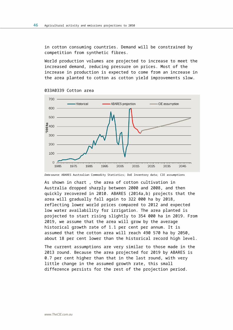
48 Agricultural activity and emissions projections to 2050
feed, and more fertiliser use in pastures, and better management practices, the growth in livestock numbers is achievable with constant, or even less, grazing land.Therefore additional land would only be required to support the projected crop production. This can come from a number of sources:■ forest conversion (or first clearing);■ re-clearing of land that had been previously cleared but reverted to
vegetation over time; or■ conversion of grazing land to cropping.Each of these is considered in more detail below.
033A0344 Total dry sheep equivalent of animals
0
50
100
150
200
250
300
350
400
450
1989 1994 1999 2004 2009 2014 2019 2024 2029 2034 2039 2044 2049
milli
on D
SE
Dairy cattle Grazing beef cattle Grain fed beef cattle Sheep Other
Data source: CIE calculation based on GMI modelling results
Projected new farming land from forest conversionDoE provided projections of first clearing (forest conversion) areas for crop and grassland up to 2050. It is projected that the annual increment in areas will peak at 27 770 ha for crops and 81 041 ha for grass by 2020, and then gradually fall to 20 757 ha for crops and 60 575 ha for grass by 2030 and stay constant thereafter.These projections suggest there will be an extra 2.5 million ha of grazing land and 0.8 ha of cropping land available in 2050 compared to 2013.These projections imply that about 1.7 million ha of farmland would be required to switch from grazing to cropping in order to satisfy cropping demand for land implied by our projection. This, judged by historical data, is feasible.
www.TheCIE.com.au

Agricultural activity and emissions projections to 2050 49
Other sources of new cropping landChart puts the cropping area and forest conversion projections in to a historical context. The left panel shows that in the past two decades the increase in cropping area has been greater than forest conversion (total accumulated increase in cropping area between 1990 and 2011 was 9.6 million ha, compared to forest conversion of 4.8 million ha). The gap between forest conversion and increased cropping area can be accounted for by conversion of grazing land and re-clearing.The right panel shows that the projected first conversion could make up 3.7 million ha of new cropping land, leaving about 1.7 million ha from other sources such as re-clearing and switching from grazing.
033A0345 Increase in cropping area and accumulated first conversion area: historical versus projection
-2
0
2
4
6
8
10
12
1990 1993 1996 1999 2002 2005 2008 2011
milli
on ha
First conversion
Increase in cropping area
-2
-1
0
1
2
3
4
5
6
2013 2018 2023 2028 2033 2038 2043 2048
First conversionIncrease in cropping area
Data source: CIE calculation based on DIICCSRTE (2013) and ABARES Australian Commodity Statistics
Chart shows the area of land cleared each year over the past 2 decades. It shows that re-clearing is a significant source of new agricultural land, in fact in recent years re-clearing has been greater than forest conversion.Since 1973 the area of land used for agriculture has decreased slightly, but the area used for cropping increased from 12 million ha in 1973 to 24 million ha in 2013. Conversion of grazing land to cropping allowed much of this increase. As a result, the share of cropping land in total agricultural land increased form 2.4 per cent in 1973 to 6.1 per cent in 2013 (chart ). Shifting land use between crops and grazing, and reversion of land to vegetation and re-clearing makes accounting for the precise make-up of the source of new agricultural land extremely difficult.However, as established above, forest conversion is not the only source of new agricultural land and therefore potential changes in farming areas,
www.TheCIE.com.au

50 Agricultural activity and emissions projections to 2050
especially cropping areas, will not be constrained by the projected forest conversion.For the purposes of estimating agricultural emissions, it is interesting to note that it is the volume of production rather than area worked that determines emissions. If land is constrained, higher production, and thus higher emissions, could be realised by using more inputs such as fertiliser, labour and capital, on a given area of land.
033A0346 Land clearing areas
0
100
200
300
400
500
600
700
1990 1992 1994 1996 1998 2000 2002 2004 2006 2008 2010
'000 h
a
Forest conversion Re-clearing
Data source: DIICCSRTE (2013)
033A0347 Total area of farms and cropping area
0
1
2
3
4
5
6
7
0
100
200
300
400
500
600
700
1972–73 1978–79 1984–85 1990–91 1996–97 2002–03 2008–09
%
milli
on ha
Total area of farms (left)% of Area used for crops (right)
Data source: CIE calculation based on ABARES Australian Commodity Statistics
www.TheCIE.com.au

Agricultural activity and emissions projections to 2050 51
5 Projected agricultural emissions
This chapter reports the agricultural emissions projections at an aggregate as well as detailed sectoral levels, noting the relative importance of different emission sources and the ways in which the projections vary from the historical record.
Emissions projections in the context of historyChart shows total agricultural emissions from 1990 to 2050. Emissions from 1990 to 2012 are based on actual values, while emissions from 2013 to 2050 are projections.Historically, total agricultural emissions have not grown strongly. Between 1990 and 2012 they fell at an average rate of around 0.3 per cent a year. This was largely due to a decline in sheep numbers and drought conditions (see the discussion below). In contrast, projected emissions are expected to grow at around 0.6 per cent a year to 2050.
044A0448 Total agricultural emissions (excluding prescribed burning of savannas): 1990 to 2050
0102030405060708090
100
1990 1995 2000 2005 2010 2015 2020 2025 2030 2035 2040 2045 2050
Mt CO
2-e
Data source: DoE emissions template, CIE projections
www.TheCIE.com.au

52 Agricultural activity and emissions projections to 2050
The broad composition of agricultural emissionsThe agricultural emissions projected here consist of six broad components:■ Enteric fermentation — the emission of methane as a by-product of the
digestive processes of cattle, sheep, pigs and other animals.■ Manure management — the emission of methane (and in some cases
nitrous oxide) from the decomposition of organic matter in animal manure.
■ Rice cultivation — methane generated during rice growing from the decomposition of residues and organic carbon in the soil as a consequence of flooding of the rice crop.
■ Agricultural soils — the emission of nitrous oxide from soils as a result of microbial and chemical transformations, due in part to the application of nitrogen fertilisers.
■ Field burning of agricultural residues — emission of a range of greenhouse gases largely as a result of stubble burning (for crops such as wheat) or burning of a sugar cane crop before harvest.
■ Lime and urea – adding lime, or dolomite to soils leads to CO2 emissions as the carbonate limes dissolve and release bicarbonate (which breaks down into CO2 and water). Applying urea to soils releases CO2 when the urea dissolves (via hydrolysis) and stimulates soil N2O emissions from soil biological activity.
Chart reports emissions for each of these sources from 1990 to 2050. Table presents key values for the projections. This shows clearly that the main reason for the decline in total emissions to 2012 was the decline in emissions from enteric fermentation.
www.TheCIE.com.au

Agricultural activity and emissions projections to 2050 53
044A0449 Emissions by broad sector 1990 to 2050
0
20
40
60
80
100
120
1990 1995 2000 2005 2010 2015 2020 2025 2030 2035 2040 2045 2050
Mt CO
2-e
Enteric Fermentation Manure ManagementRice Cultivation Agricultural SoilsField burning of agricultural residues Lime and Urea
Data source: DoE emissions template, CIE projections
044B0450 Emissions by broad sector1990 2012 2020 2030 2050
Mt CO2-e Mt CO2-e Mt CO2-e Mt CO2-e Mt CO2-eEnteric fermentation 67.29 56.27 56.70 59.93 67.75Manure management 2.77 3.63 3.85 4.11 4.63Rice cultivation 0.65 0.59 0.70 0.70 0.70Agricultural soils 9.33 11.00 11.05 12.05 13.82Field burning of agricultural residues
0.29 0.52 0.52 0.62 0.79
Lime and urea 0.53 3.14 3.48 3.91 4.43Total 80.85 75.15 76.30 81.32 92.12Data source: DoE emissions template, CIE projections
Overview of emissions by sector and subsectorTable summarises the emissions projections for each emissions sector and subsector of the Australian emissions inventory.Several points emerge from this table.■ Enteric fermentation is the major source of emissions. Within this, most
emissions come from grazing beef cattle (59 per cent in 2020, for example) followed by sheep (23 per cent in 2020).
■ Within manure management (which is around 5.2 per cent of total emissions), just over a third of emissions come from pigs, followed by grain fed cattle, poultry and dairy cattle (the order of grain fed cattle
www.TheCIE.com.au

54 Agricultural activity and emissions projections to 2050
and poultry is expected to change by around 2050 due to faster growth in poultry meat production).
■ Agricultural soil emissions are 14 per cent of total agricultural emissions in 2020 and 16 per cent in 2050. Within this, crop residue emissions are the largest component (accounting for 44 per cent in 2020 and 47 per cent in 2050).
■ Rice cultivation accounts for just 0.8 per cent of total agricultural emissions.
■ Field burning of agricultural residues accounts for less than 1 per cent of total agricultural emissions, with the wheat sector accounting for almost half of this.
■ Lime and urea account for 4.6 per cent of total agricultural emissions in 2020 and 4.8 per cent in 2050.
044B0451 Agricultural emissions by sector and subsector1990 2012 2020 2030 2050
Mt CO2-e Mt CO2-e Mt CO2-e Mt CO2-e Mt CO2-eEnteric Fermentation 67.29 56.27 56.70 59.93 67.75 Cattle 37.96 43.37 43.33 46.37 53.42
Dairy Cattle 6.67 7.06 7.57 7.74 8.28Grazing beef cattle 30.91 34.16 33.63 36.40 42.78Grain fed cattle 0.38 2.16 2.13 2.23 2.36
Sheep 28.95 12.58 13.04 13.21 13.92Swine 0.10 0.08 0.08 0.09 0.10Other 0.28 0.23 0.25 0.27 0.30Manure Management 2.77 3.63 3.85 4.11 4.63Cattle 0.77 1.64 1.67 1.73 1.84
Dairy Cattle 0.58 0.61 0.66 0.67 0.72Grazing beef cattle 0.02 0.02 0.02 0.03 0.03Grain fed cattle 0.17 1.00 0.99 1.03 1.09
Sheep 0.01 0.00 0.00 0.00 0.00Swine 1.57 1.27 1.33 1.44 1.67Poultry 0.42 0.73 0.85 0.93 1.11Other 0.00 0.00 0.00 0.00 0.00Rice Cultivation 0.65 0.59 0.70 0.70 0.70Agricultural Soils 9.33 11.00 11.05 12.05 13.82Animal Production 4.71 3.59 3.64 3.83 4.30Direct soil emissions 2.13 4.88 4.87 5.51 6.48Indirect soil emissions 2.49 2.53 2.54 2.71 3.03Field burning of agricultural residues 0.29 0.52 0.52 0.62 0.79
www.TheCIE.com.au

Agricultural activity and emissions projections to 2050 55
Wheat 0.12 0.26 0.23 0.28 0.38Maize 0.01 0.01 0.01 0.01 0.02Sugar Cane 0.04 0.04 0.04 0.05 0.05Other 0.05 0.09 0.09 0.11 0.15Rice 0.05 0.05 0.07 0.07 0.08Pulse 0.02 0.04 0.06 0.08 0.10Peanuts 0.00 0.00 0.00 0.00 0.00Other Crops 0.00 0.02 0.02 0.02 0.03Lime and Urea 0.53 3.14 3.48 3.91 4.43Total 80.85 75.15 76.30 81.32 92.12Note: All emissions are calculated using AR4 global warming potentials. Average emission reported. Results for 2012 are actual.Data source: DoE emissions template, CIE projections
Livestock related emissionsChart summarises the history and projections for livestock related emissions.6 Enteric fermentation is the largest source of these. Variations in enteric fermentation emissions largely explain total changes in emissions. While these fell at around 0.8 per cent a year historically (to 2012), over the projection period they are expected to grow at around 0.5 per cent a year.
044A0452 Livestock emissions
0
10
20
30
40
50
60
70
80
90
1990 1995 2000 2005 2010 2015 2020 2025 2030 2035 2040 2045 2050
Mt CO
2-e
Enteric Fermentation Manure Management Agricultural Soils
Note: All emissions are calculated using AR4 global warming potentials. Average emission reported.Data source: DoE emissions template, CIE projections
6 Strictly speaking, part of the CO2 emissions from lime and urea application should be attributed to livestock too, however, the Department has not included this detail as the emissions are relatively small.
www.TheCIE.com.au

56 Agricultural activity and emissions projections to 2050
Enteric fermentationChart provides the history and projections for enteric fermentation emissions. This chart shows clearly that the reason for the historical decline in enteric fermentation emission was the decline in emission from sheep — other sources have tended to be constant or increase slightly over time. Historically, enteric fermentation from sheep declined at around 3.7 per cent a year. However, these emissions are projected to increase at a rate of around 0.3 per cent a year over the projection period. This is a consequence of an expected recovery in sheep numbers due to better wool prices and increased revenues from meat production.Historically, enteric fermentation from grazing beef cattle increased at around 0.5 per cent a year. Some of this growth was constrained by drought (and flood) conditions. These emissions are projected to grow at 0.6 per cent a year over the projection period. This is due largely to relatively strong projected beef exports, particularly to rapidly growing Asian economies. In addition, the projections do not incorporate the implications of potential future droughts.
044A0453 Enteric fermentation
0
10
20
30
40
50
60
70
80
1990 1995 2000 2005 2010 2015 2020 2025 2030 2035 2040 2045 2050
Mt CO
2-e
Dairy Cattle Grazing beef cattle Grain fed cattle Sheep Other
Note: Other includes swine and otherData source: DoE emissions template, CIE projections
Enteric fermentation emissions from dairy cattle grew at around 0.3 per cent a year historically, and this is projected to continue at around 0.4 per cent a year over the projection period.
Manure managementChart shows projections for livestock emissions related to manure management. The pattern for each of these components varies, particularly when compared with historical emissions.
www.TheCIE.com.au

Agricultural activity and emissions projections to 2050 57
044A0454 Manure management
0
1
2
3
4
5
1990 1995 2000 2005 2010 2015 2020 2025 2030 2035 2040 2045 2050
Mt CO
2-e
Dairy Cattle Grain fed cattle Swine Poultry Other
Note: Other includes grazing beef cattle, sheep and otherData source: DoE emissions template, CIE projections
For example, while emissions from grain fed beef historically grew rapidly (at 8.4 per cent a year) this is expected to stabilise at around 0.2 per cent a year over the projection period. In contrast, emissions associated with dairy cattle are expected to be little bit higher than historic growth rates (0.4 per cent versus 0.3 per cent).
Agricultural soilsChart summarises emissions from agricultural soils. These relate to both animal and crop production. Historically crop residue has been the fastest growing source within this category and it is expected to remain so, albeit with a much slower growth rate than historically (projected to be 0.7 per cent compared to 3.8 per cent a year in the past).
www.TheCIE.com.au

58 Agricultural activity and emissions projections to 2050
044A0455 Agricultural soils
0
2
4
6
8
10
12
14
16
18
1990 1995 2000 2005 2010 2015 2020 2025 2030 2035 2040 2045 2050
Mt CO
2-e
Indirect soil emissionsCrop Residue EmissionsAnimal Production: Nitrogen excreted on pasture range and paddock
Note: All emissions are calculated using AR4 global warming potentials. Average emission reported.Data source: DoE emissions template, CIE projections
Crop emissionsChart summarises crop emissions. These mostly arise through agricultural soils and historically have been greatly influenced by drought. The effect of the millennial drought is very clear in the historical values. Despite the disruptions from drought which are not incorporated in the projections, crop emissions are projected to grow at slightly larger than third of the overall historic average rate (0.7 per cent a year, compared with 2.0 per cent a year historically).Chart shows emission from field burning of agricultural residues. These are due mostly to wheat and, to a slightly lesser extent, a combination of other crops. As before, the effects of drought are very evident in the historical emissions. The projected cumulative average growth rate (CAGR) of emissions for wheat (around 1.0 per cent a year) is about third of the average historical growth (of around 3.4 per cent a year). However, comparing the historical and future trends in emissions abstracting from the effects of drought, shows that the projected future growth (around 1.6 per cent a year) is closer to the historical trend growth (around 2.5 per cent a year).
www.TheCIE.com.au

Agricultural activity and emissions projections to 2050 59
044A0456 Crop emissions
0
2
4
6
8
10
12
1990 1995 2000 2005 2010 2015 2020 2025 2030 2035 2040 2045 2050
Mt CO
2-e
Rice Cultivation Agricultural Soils Field burning residues
Note: All emissions are calculated using AR4 global warming potentials. Average emission reported.Data source: DoE emissions template, CIE projections
044A0457 Field burning of agricultural residues
0.0
0.1
0.2
0.3
0.4
0.5
0.6
0.7
0.8
0.9
1990 1995 2000 2005 2010 2015 2020 2025 2030 2035 2040 2045 2050
Mt CO
2-e
Wheat Sugar Cane Rice Other
Note: Other includes maize, pulses, peanuts and other cropsData source: DoE emissions template, CIE projections
www.TheCIE.com.au

60 Agricultural activity and emissions projections to 2050
6 Sensitivity analysis
The simulated outcomes from the economic models used as the basis for the emissions projections depend on a variety of ‘exogenous’ (or ‘outside’) input assumptions. The assumptions used are plausible future outcomes, partly based on historical observations, but the future values are not known with certainty. This chapter reports results from sensitivity analysis around a number of the key input assumptions.
Variables for sensitivity analysisSensitivity analyses are conducted for several key variables affecting agricultural production and emissions as summarised in table . Each of these are investigated separately as well as being combined to establish upper and lower bounds for emissions projections.
055B0558 Individual sensitivity analysesSensitivity Shock variable Magnitude
Foreign income Annual growth rate in foreign income
20 per cent deviation from the central reference case assumption
Exchange rate Australian exchange rate 20 per cent deviation from the central reference case assumption as provided by DoE. Note that this 20 per cent variation is defined in terms of USD/AUD.
Productivity Annual growth rate in Australian agricultural productivity
50 per cent deviation from the central reference case assumption
Slaughtering weight/yield Annual growth rate in slaughtering weight for beef, milk yield for dairy cattle and yield for crops
50 per cent deviation from the central reference case assumption
Input cost Agricultural input prices 20 per cent deviation from the central reference case assumption
Lower supply responsiveness Supply elasticities Halve the relevant supply
www.TheCIE.com.au
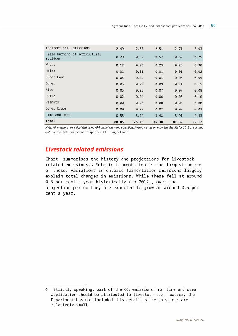
Agricultural activity and emissions projections to 2050 61
elasticities (see Appendix A for elasticity values)
Combined sensitivities Combination of foreign income, exchange rate, productivity, slaughter weight/yield, input prices and lower supply responsiveness.
Individual factors arranged to lead to the same directional impact on emissions, that is, high (low) foreign income and productivity being joined by low (high) slaughtering weight/yield and input prices.
Source: CIE construction in consultation with DoE
Each of these variables was chosen for the sensitivity analysis as they are all important drivers of agricultural output and therefore emissions. The values chosen for the sensitivity analysis are within observed historical variations. They do not seek to capture the entire extent of possible variation, including extreme values, but do roughly cover a range of reasonable variation.
Sensitivity analysis resultsTable reports the percentage deviation of each sensitivity scenario from the central reference case for selected projection years.
055B0559 Impact on emissions – percentage deviation from the central reference case
2015 2020 2030 2050
Foreign income High 0.32 1.29 3.30 7.54 Low -0.41 -1.37 -3.31 -7.09Exchange rate High -8.01 -7.98 -7.97 -8.01 Low 10.78 10.75 10.76 10.84Productivity High 0.51 1.71 4.19 9.53 Low -0.49 -1.66 -3.99 -8.56Slaughtering weight/yield High -1.10 -2.52 -5.29 -8.71 Low 1.14 2.63 5.74 9.94Input cost High -1.41 -2.57 -3.60 -4.97 Low 1.56 2.76 3.86 5.37Supply responsiveness
www.TheCIE.com.au
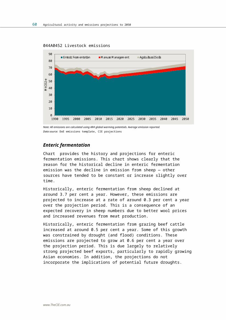
62 Agricultural activity and emissions projections to 2050
Low -0.04 -3.53 -6.32 -10.31Combined High 14.39 14.96 20.60 31.78 Low -10.76 -17.14 -25.02 -36.06Note: The ‘high’s and ‘low’s under each sensitivity refer to the high and low values of shocked variables, while the high and low under the combined scenario refer to the high and low emissions.Source: CIE Grains, Dairy and GMI simulations
Several points emerge from these results.■ The largest impact in the short term (2015 and 2020) comes from
variations in the exchange rate. As explained in chapter 3, a depreciation of the Australian dollar will increase Australian production (and therefore emissions) by encouraging more demand for Australian products. In 2020, for example, a more favourable exchange rate could lead to an 11 per cent increase in emissions (relative to the central reference case). A less favourable exchange rate could lead to an 8.0 per cent decline in emissions7.
■ The impact of the exchange rate variation is the greatest in the short term, by a significant margin, because the variation is a 20 per cent deviation each year of the projection, rather than a change in growth rates as assumed for the other variables which accumulates over the projection period.
■ Different input costs could lead to a variation in emissions (up or down) of around 2.6 per cent by 2020. An increase in costs will tend to lower production and therefore emissions. The results in table show that the impact of higher and lower input costs is not as significant in the longer term (2030 and 2050) as other variables, despite appearing significant in the short term results. This is a function of the relative growth rates assumed for each of the variables.
■ The impact of productivity assumptions is very similar to that of slaughter weight and yield assumptions. In 2030, higher (lower) productivity lead to emissions 4.2 per cent higher (4 per cent lower) and higher (lower) slaughter weights and yields leads to emissions 5.3 per cent lower (5.7 per cent higher).
■ The combination of sensitivities suggests that in 2020, emissions could vary by 15-17 per cent around the central reference case. By 2030 the variation could be around 20 to 25 per cent. Central case assumptions lead to a projected increase in agricultural emissions . However, under a certain set of reasonable assumptions (the combined low case scenario), emissions from agriculture could remain unchanged, or even decline slightly from current levels over the forecast period.
7 Note that as pointed out above, these exchange rate deviations are not equal because exchange rates are expressed in AUD/USD terms within the models.
www.TheCIE.com.au

Agricultural activity and emissions projections to 2050 63
Changes to the assumptions tested in the sensitivity analyses may have implications for the amount of land used for agricultural production. For example, a decline in productivity or yield in grains leads to greater demand for land, as does increased foreign income – driving increased production of grains and livestock products. The range of production, however, is still considered feasible given the amount of land available (see discussion in chapter 3) through market driven adjustments and switching of land between agricultural activities. For example, increased livestock production is likely to be realised through greater pasture utilisation and more grain finishing. The combination of sensitivity results that lead to the greatest increase in land required for cropping would require an additional 2.5 million hectares. This land could be made available from switching land from pastures to cropping, while maintaining (or increasing) livestock production through grain finishing and greater pasture utilisation. In general, increased agricultural production is likely to lead to more intensive agricultural production, thus not requiring significantly greater areas of land.Details on each of the individual sensitivities are provided in the remainder of this chapter.
Foreign incomeAustralian agricultural sectors are highly exposed to export markets and export demand is a key driver of much of Australian agricultural activity. Fluctuations in foreign markets will have significant impacts on domestic production. Typically, foreign demand is determined by foreign population and income levels. Variation in population projections are small in general and thus have not been considered for this exercise. Projections of income growth in trading partner countries reasonably vary over time and between different forecasting methodologies. They are also inherently uncertain due to uncertainties in the international environment. Consequently, as shown in table , the sensitivity analysis of foreign demand is modelled by different assumptions about the annual growth in foreign income. This sensitivity tests the impact of a 20 per cent variation in income growth rates. Observed adjustments in projected economic growth rates are often of the order of 20 per cent. In July 2014 the IMF released an update to their April World Economic Outlook (IMF 2014c). Projected economic growth rates for 2014 and 2015 were revised for each country and region. The revised growth rates differed from the April projections by up to 500 per cent for some countries. The estimated growth rate for global output was revised down by 8.8 per cent.Chart shows the impact of changing foreign income on Australia’s major agricultural outputs. In general the higher the foreign income, the higher the output. The impacts on grains production are smaller than those for
www.TheCIE.com.au
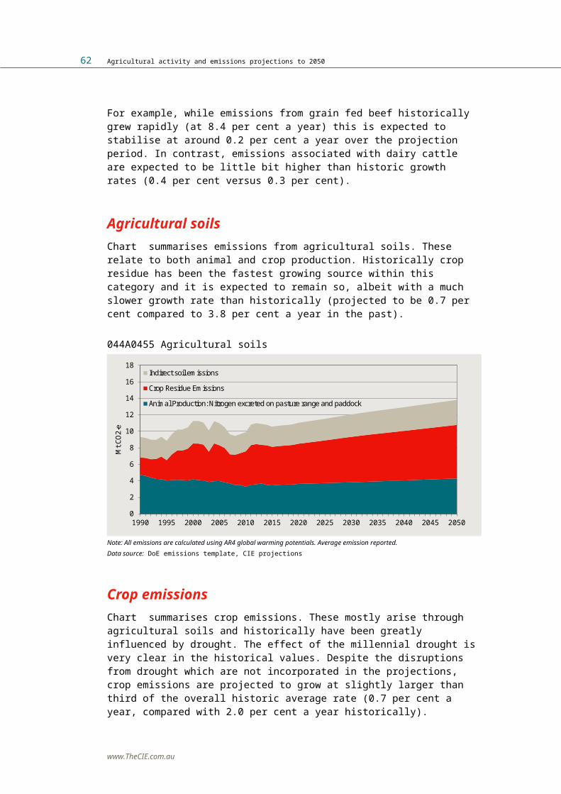
64 Agricultural activity and emissions projections to 2050
livestock products because meat and dairy products are relatively more luxurious goods, with high income elasticities of demand, meaning a change in incomes leads to greater impacts on demand.The resulting impact of the variation in foreign income levels on total agricultural emissions is shown in chart .
055A0560 Impact of foreign income sensitivity on annual emissions
Data source: CIE Grains, Dairy and GMI simulations
www.TheCIE.com.au

Agricultural activity and emissions projections to 2050 65
055C0561 Impact of foreign income on agricultural output
Data source: CIE Grain, Dairy and GMI model simulations
www.TheCIE.com.au

66 Agricultural activity and emissions projections to 2050
Exchange ratesLike income, exchange rates are inherently difficult to forecast but they have major implications for export industries — both in terms of their competitiveness and in terms of how foreign income translates into Australian dollars. A higher Australian dollar means higher prices for Australian exports and cheaper prices for imports, leading to lower demand for Australian products. On the other hand, a lower Australian dollar would boost the demand for Australian products.This sensitivity tests the implications of a 20 per cent variation in the baseline exchange rate values. Note that this variation is defined around an exchange rate defined in USD/AUD terms. While the deviations up and down from the central case are equal when expressed in this way, they are not equal when expressed as AUD/USD. This latter expression of the exchange rate is implemented in the economic models. Examining historical exchange rates show that the average annual exchange rate has varied by up to 22 per cent from year to year (ABARES 2013).Chart illustrates how the variation in exchange rates are projected to impact agricultural activity levels. As all these agricultural goods are highly traded, the exchange rate has similar impacts on activity levels for each of the sectors. Chart shows the resulting impact on total agricultural emissions.
055A0562 Impact of the exchange rate sensitivity on annual emissions
Data source: CIE Grains, Dairy and GMI simulations
www.TheCIE.com.au

Agricultural activity and emissions projections to 2050 67
055C0563 Impact of exchange rates on agricultural output
Data source: CIE Grain, Dairy and GMI model simulations
www.TheCIE.com.au

68 Agricultural activity and emissions projections to 2050
ProductivityAgricultural productivity varies over time, most frequently due to climatic conditions. Large variations in productivity are common in the historical record. Measuring productivity is also challenging and can be done in different ways. This sensitivity tests the implications of a 50 per cent variation in assumed productivity growth.As an example of the fluctuation in productivity growth, average growth for the agriculture sector between 1995 and 2000 was 2.6 per cent per annum, while it was only 0.9 per cent per annum between 2000 and 2012 (ABS 2013b).The ABS and ABARES have different estimates of historical productivity growth rates. For the period 2000 to 2011, ABARES estimated productivity growth averaged -0.3 per cent (Dahl et al 2013) (compared to 0.89 per cent for agriculture between 2000 and 2012 estimated by ABS).Chart reports the agricultural activities under different assumptions of productivity growth. Higher productivity improvements bring about greater cost reductions (and hence lower prices) leading to greater consumption and production. Chart shows the resulting impact on total agricultural emissions.
055A0564 Impact of the productivity sensitivity on annual emissions
Data source: CIE Grains, Dairy and GMI simulations
www.TheCIE.com.au

Agricultural activity and emissions projections to 2050 69
055C0565 Impact of productivity on agricultural output
Data source: CIE Grain, Dairy and GMI model simulations
www.TheCIE.com.au

70 Agricultural activity and emissions projections to 2050
Slaughtering weight and yieldSlaughter weights, milk yields and crop yields are a subset of productivity and also vary over time. The impacts on animal numbers and on grain production are in opposing directions. Higher slaughtering weights in the meat industry and higher milk production per cow in the dairy industry mean that, for a certain output, fewer animals are needed. As shown by the top 6 diagrams in chart , higher (lower) growth in slaughtering weight/yield is associated with lower (higher) animal numbers.By contrast, higher yields in grain production mean more production is possible for a given amount of land, leading to the same implications as a productivity improvement in the sector. As shown in the bottom 2 diagrams in the chart, higher (lower) yield growth is associated with higher (lower) grain production.This sensitivity tests the implications of a 50 per cent variation in assumed growth for these variables. The magnitude of the chosen variations are within observed historical variations. As an example, this can be observed in chart which plots the historical growth in beef slaughtering weights and the assumed growth rate under the central, high and low scenarios modelled.Chart reports the agricultural activities under different assumptions of the growth in slaughtering weight and yield and chart shows the associated impacts on emissions.The dairy industry stands out in the sensitivity analysis – dairy cattle numbers would fall if the yield growth rate is 50 per cent higher than the assumed growth in the central reference case. This is partly due to the relatively high growth assumption of yield in dairy industry compared with other industries in the central reference case.
www.TheCIE.com.au

Agricultural activity and emissions projections to 2050 71
055A0566 Growth rate in beef slaughter weights, historical and assumed future rates
Data source: ABARES Australian Commodity Statistics 2013 and the CIE
055A0567 Impact of the slaughtering weight/yield sensitivity on annual emissions
Data source: CIE Grains, Dairy and GMI simulations
www.TheCIE.com.au

72 Agricultural activity and emissions projections to 2050
055C0568 Impact of slaughtering weight and yield on agricultural output
Data source: CIE Grain, Dairy and GMI model simulations
www.TheCIE.com.au

Agricultural activity and emissions projections to 2050 73
Input pricesInput costs, while often less variable than other factors associated with agriculture, are nevertheless subject to a number of uncertainties. This sensitivity tests the implications of a 20 per cent variation in assumed input cost changes. All the variable input prices were altered, including hired labour, fertiliser, feed, and fuel and electricity.ABARES (2013) data on farm costs show that from year to year over the past 15 years, total farm costs increased on average, 3.1 per cent a year. However, the actual change in farm costs from one year to the next ranged from a fall of 5.9 per cent to an increase of 18 per cent. A 20 per cent variation in input costs is within this observed historical variation.Chart reports the agricultural activities under different assumptions of the prices of inputs into the production system. The impact is opposite to that from a productivity improvement. Higher input prices mean higher cost of a product, depressing demand and thus production. The impact on emissions is shown in chart .
055A0569 Impact of the input price sensitivity on annual emissions
Data source: CIE Grains, Dairy and GMI simulations
www.TheCIE.com.au

74 Agricultural activity and emissions projections to 2050
055C0570 Impact of input prices on agricultural output
Data source: CIE Grain, Dairy and GMI model simulations
www.TheCIE.com.au

Agricultural activity and emissions projections to 2050 75
Lower supply responsivenessClimatic conditions, particularly drought, have a major influence on agricultural output. In this sensitivity we test a permanently reduced elasticity of supply — that is, a reduced ability of each of the agricultural sectors to respond to changes in demand. This sensitivity seeks to shed light on the possible implications of extended periods of low rainfall or drought conditions. There are several ways to model the impact of drought, and a common way is through reductions in productivity (yields). As the impact of different productivity assumptions has been investigated separately, we adopt an alternative approach that lowers the supply responsiveness of the agriculture sector. This approach is taken as we often observe lower output and higher prices in a drought, that is, a higher price is required to encourage farmers to produce the same amount of products – a lower supply elasticity. The supply elasticities under the sensitivity are half the value used in the central simulations. This is designed to simulate the inability of agricultural industries to respond to changes in external factors such as demand.Chart reports the agricultural activities under the lower supply responsiveness case along with the central reference case. As expected, this sensitivity results in lower output of each commodity compared with the central reference case. The impact on agricultural emissions is shown in chart .
055A0571 Impact of the lower supply response sensitivity on annual emissions
Data source: CIE Grains, Dairy and GMI simulations
www.TheCIE.com.au

76 Agricultural activity and emissions projections to 2050
055C0572 Impact of lower supply responsiveness on agricultural output
Data source: CIE Grain, Dairy and GMI model simulations
www.TheCIE.com.au
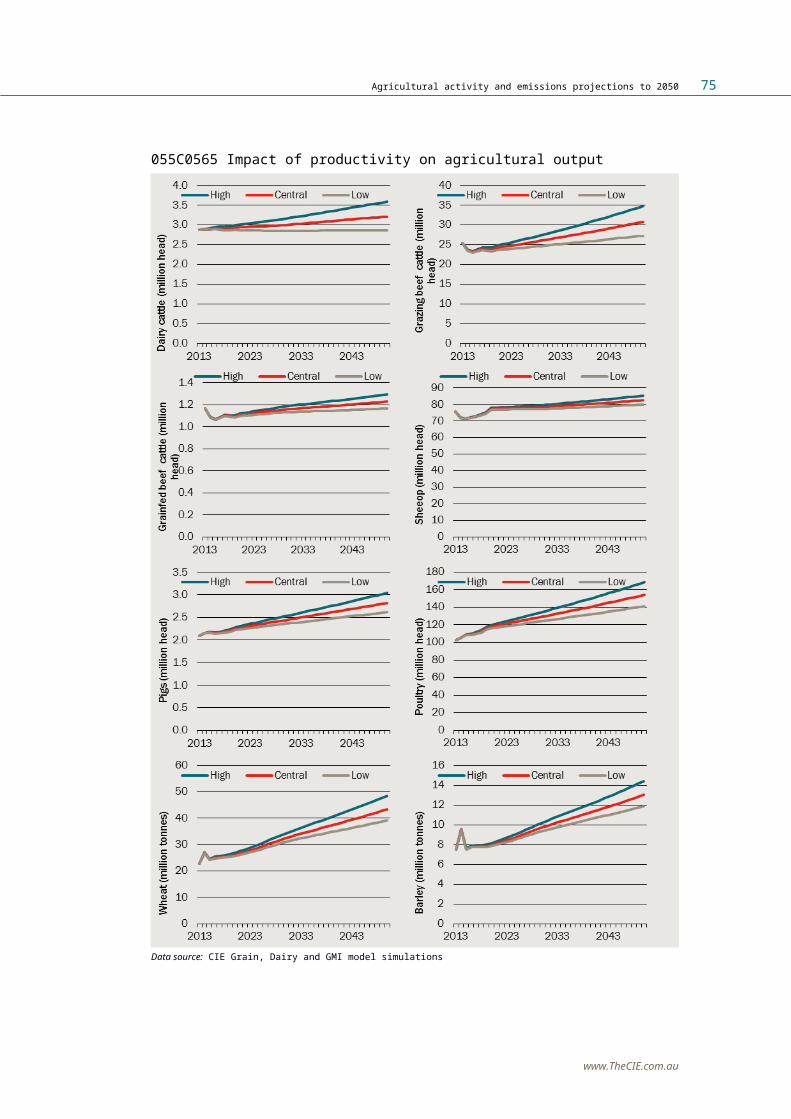
Agricultural activity and emissions projections to 2050 77
Combined sensitivity analysisChart reports the sensitivity analysis results of combining the foreign income, productivity, slaughtering weight/yield, input price and supply responsiveness sensitivities together.It can be seen from the chart that in general animal numbers are more sensitive compared to grain production. The dairy cattle numbers appear to be the most sensitive with a deviation of up to 46 per cent by 2050, followed by poultry numbers with a deviation of up to 40 to 44 per cent by 2050. Overall, grain production is less sensitive to the assumptions tested. This is mainly driven by significantly lower sensitivity to foreign income changes, and to a lesser extent exchange rate changes. Grains are a staple, low cost food and so the demand for these products is less sensitive to changes in price and income than luxury livestock products.The overall impact on agricultural emissions is shown in chart . This chart shows that under the sensitivities, in 2020, emissions could vary by 15-17 per cent around the central reference case. By 2050 the variation could be around 32 to 36 per cent. Most of the assumptions used indicate that agricultural emissions are expected to increase over time. These sensitivity results however show that, with alternative assumptions, emission levels projected for 2050 may be the same as, or even lower than, current agricultural emission levels.
055A0573 Combined impact of sensitivity analysis on annual emissions
Note: The high and low under the combined scenario refer to the high and low emissions.Data source: CIE Grains, Dairy and GMI simulations
www.TheCIE.com.au
78 Agricultural activity and emissions projections to 2050
055C0574 Combined sensitivity analysis result
Data source: CIE Grain, Dairy and GMI model simulations
www.TheCIE.com.au

Agricultural activity and emissions projections to 2050 79
References
ABARES 2014a, Australian commodities, March Quarter 2014, available at http://data.daff.gov.au/data/warehouse/agcomd9abcc004/agcomd9abcc004201403/AgCommodities2014.No1_Ver1.1.0.pdf
ABARES 2014b, Australian commodities, September Quarter 2014, available at http://data.daff.gov.au/data/warehouse/agcomd9abcc004/agcomd9abcc201409/AgCommodities201409_1.0.0.pdf
ABARES 2013, Australian commodity statistics, Canberra.ABS 2013a, Population Projections, Australia, 2012 (base) to 2101, Cat.No.3222.0ABS 2013b, Estimates of Industry Multifactor Productivity, Cat. No.5260.0.55.002CIE 2013, Australian agricultural emissions projections: To 2050, Report to
Department of Industry, Innovation, Climate Change, Science, Research and Tertiary Education, Canberra.
Dahl, A, R. Leith and E. Gray 2013, ‘Productivity in the broadacre and dairy industries’, Agricultural commodities, 3(1), March, pp200-220.
Dairy Australia 2014, National Dairy Farmer Survey 2014, available at http://www.dairyaustralia.com.au/Markets-and-statistics/Market-situation-and-outlook/National-Dairy-Farmer-Survey.aspx
Deads, B., D. Mobsby, N. Thompson and A. Dahl 2013, Australian grains: Outlook for 2013-14 and industry productivity, ABARES report prepared for the Grains Research and Development Corporation, Canberra, November.
Department of Environment (DoE) 2014, National Greenhouse Gas Inventory – Agriculture, spreadsheet provided to the CIE
Department of Industry, Innovation, Climate Change, Science, Research and Tertiary Education (DIICCSRTE) 2013, Australian National Greenhouse Accounts: Australian Land Use, Land Use Change and Forestry Emissions Projections to 2030, Canberra, available at http://www.environment.gov.au/climate-change/publications/australian-land-use-land-use-change-and-forestry-emissions-projections-2030
International Monetary Fund (IMF) 2014a, World Economic Outlook: Recovery Strengthens, Remains Uneven, April 2014, IMF, Washington D.C., available at http://www.imf.org/external/pubs/ft/weo/2014/01/
International Monetary Fund (IMF), 2014b, World Economic Outlook Database, April, available at http://www.imf.org/external/pubs/ft/weo/2014/01/weodata/index.aspx
International Monetary Fund (IMF), 2014c, World Economic Outlook Update: An uneven global recovery continues, July, available at http://www.imf.org/external/pubs/ft/weo/2014/update/02/
McKibbin, W. and P. Wilcoxen, 1999, ‘The theoretical and empirical structure of the G-Cubed model’, Economic Modelling, 16(1), pp123-48.
www.TheCIE.com.au

80 Agricultural activity and emissions projections to 2050
Narayanan, G., A.A. Badri and R. McDougall, Eds, 2012, Global Trade, Assistance, and Production: The GTAP 8 Data Base, Center for Global Trade Analysis, Purdue University.
Productivity Commission 2006, Potential Benefits of the National Reform Agenda, Report to the Council of Australian Governments, available at http://www.pc.gov.au/research/commissionresearch/nationalreformagenda
Revelant, L., Hardy, S. and Sanderson, G. 2004, How to manage soil for citrus, New South Wales Department of Primary Industries, available at: http://www.dpi.nsw.gov.au/agriculture/horticulture/citrus/management/other-information/soil
Treasury and Department of Industry, Innovation, Climate Change, Science, Research and Tertiary Education 2013, Climate Change Mitigation Scenarios: modelling report provided to the Climate Change Authority in support of its Caps and Target review, Available at http://www.environment.gov.au/node/35527
Tulloh, C., Jian, T. and Pearce, D. 2014, The impact of free trade agreements on Australia: A model-based analysis, RIRDC publication No. 14/002, Rural Industries Research and Development Corporation, Canberra, February.
United Nations, Department of Economic and Social Affairs, Population Division 2013, World Population Prospects: The 2012 Revision, DVD Edition.
www.TheCIE.com.au
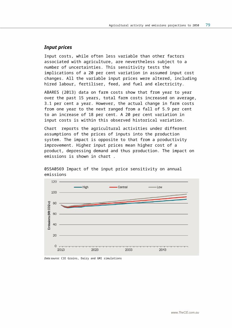
Agricultural activity and emissions projections to 2050 81
A Modelling approach
Projection frameworkThe projections are prepared using a suite of economic models to project Australian agricultural production and emissions. These models include:■ General equilibrium model of the global economy – CIE G-Cubed■ General equilibrium model of the Australian economy – Food Processing
(FP) version of the CIE-Regions model■ Commodity models – GMI, Dairy, Grains, Sugar, Rice and CottonThese models are run in sequential order from global to national to commodity.The CIE G-Cubed model is used to project external demand for Australian goods and services and international prices with assumptions about global economic and population growth and trade policy development such as Australia’s free trade agreements with Korea and Japan.The results from CIE G-Cubed, together with assumptions of economic and population growth and productivity improvement in Australian states and territories, are then fed into the FP model to project the production and prices for broad commodities as identified in the model.The global and Australian CGE modelling results, together with other commodity specific assumptions, are then fed into the commodity models to project commodity production, animal numbers and associated inputs such as fertiliser use.These agricultural activity information are then input into the spreadsheet template provided by DoE to produce emissions projection.Finally, sensitivity analysis is carried out to test how the projection results are affected by the assumptions of key variables and parameters. The sensitivity analysis takes two forms:■ Test the impact of a particular variable/parameter on the projected
output or emissions;■ Combine the key variables and parameters together to form high and
low projections
www.TheCIE.com.au

82 Agricultural activity and emissions projections to 2050
Economic models
CIE G-CubedDeveloped by Professors Warwick McKibbin and Peter Wilcoxen, G-Cubed is a dynamic general equilibrium model of the world economy (McKibbin and Wilcoxen 1999). It connects two strands of quantitative economic modelling – traditional multisectoral general equilibrium models which capture sectoral linkages and interactions and macroeconomic models which are mostly dynamic and have full macroeconomic closure.The key features of G–Cubed are that it:■ specifies the demand and supply sides of economies;■ integrates the real and financial markets of these economies;■ fully accounts for stocks and flows of real resources and financial
assets;■ imposes intertemporal budget constraints so that agents and countries
cannot indefinitely borrow and lend without undertaking the resource transfers necessary to service outstanding liabilities;
■ has short run behaviour that is a weighted average of neoclassical optimising behaviour and liquidity constrained behaviour;
■ has a real side that is disaggregated to allow for production and trade of multiple goods and services within and between economies;
■ has full short and long run macroeconomic closure with annual macrodynamics around a neoclassical growth model; and
■ can be solved for the full rational expectations equilibrium annually.While maintaining these features, the CIE’s inhouse model of G-Cubed, CIE G-Cubed, has more detailed, and more flexible, coverage of countries and industries to be fully compatible with the GTAP database. The latest version (Version 8) of GTAP database has identified 129 countries/country groups for all 57 GTAP sectors/commodities (Narayanan et al. 2012).For this project, the 129 countries/country groups are aggregated into seven economies: Australia, China, India, Rest of Asia, United States, European Union, and Rest of the World, while keeping all the 57 sectors (table ).
Food Processing (FP) modelThe Food Processing (FP) model is a special version of the CIE-Regions model, which provides a detailed account of the Australian agriculture and food value chain with 10 farming sectors and 11 food manufacturing sectors while aggregating other sectors (see table ).
www.TheCIE.com.au
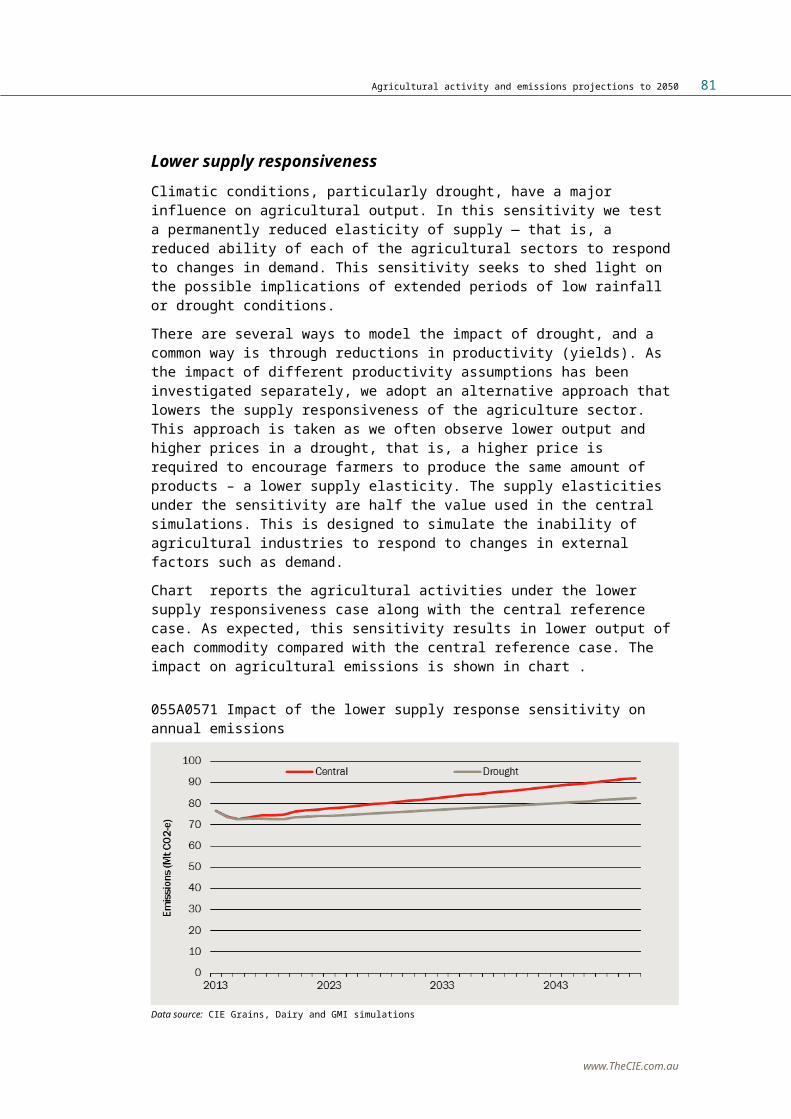
Agricultural activity and emissions projections to 2050 83
A11AA175 Sectors identified in CGE modelsCIE G-Cubed FP model
Paddy Rice Other Transport Equipment CattleWheat Electronic Equipment SheepOther Grains Other Machinery & Equipment Dairy cattleVeg & Fruit Other Manufacturing Other animalsOil Seeds Electricity WheatCane & Beet Gas Distribution OilseedPlant Fibres Water Other grainsOther Crops Construction Fruits and nutsCattle Trade VegetablesOther Animal Products Other Transport Other cropsRaw Milk Water Transport ForestryWool Air Transport FishingForestry Communications MiningFishing Other Financial Intermediation BeefCoal Insurance Sheep meatOil Other Business Services Dairy products – freshGas Recreation & Other Services Dairy products –
manufacturingOther Mining Other Services (Government) Flour, confectionary and
bakeryCattle Meat Dwellings Oil and fatOther Meat JuiceVegetable Oils Fruit productsMilk Vegetable productsProcessed Rice Other food manufacturingSugar Beverage and tobaccoOther Food Wood and paper productsBeverages & Tobacco Petrol productsTextiles ChemicalsWearing Apparel Other ManufacturingLeather Electricity GenerationLumber ElectricityPaper & Paper Products GasPetroleum & Coke Water
www.TheCIE.com.au

84 Agricultural activity and emissions projections to 2050
Chemical Rubber Products ConstructionNon-Metallic Minerals WholesaleIron & Steel Retail TradeNon-Ferrous Metals TransportFabricated Metal Products ServicesMotor Vehicles DwellingsSource: CIE
The model is a general equilibrium model of the Australian economy. It was developed by the CIE based on the publicly available MMRF-NRA model developed for the Productivity Commission (2006) by the Centre for Policy Studies8. The CIE has updated the model and introduced more detailed treatment of state/territory government fiscal revenues and expenditures.Some of the key features of the model are that it:■ provides a detailed account of industry activity, investment, imports,
exports, changes in prices, employment, household spending and savings and many other factors;
■ identifies 38 industries and commodities (see table );■ accounts for Australia’s six states and two territories as distinct regions
including specific details about the budgetary revenues and expenditures of each of the eight state and territory governments and the Australian Government (the government finances in the FP model align as closely as practicable to the ABS government finance data);
■ includes a detailed treatment of the fiscal effects of the Goods and Services Tax (GST);
■ specifically accounts for major taxes including land taxes, payroll taxes, stamp duties and others at the state level, as well as income taxes, tariffs, excise, the GST and other taxes at the federal level;
■ traces out the impact of transfers between governments;■ accounts for differing economic fundamentals in the states (for
instance, the mining boom in WA and Queensland);■ can produce results on employment and value added at a regional
level; and■ can be run in a static or dynamic mode. The dynamic version allows the
analysis to trace impacts over time as the economy adjusts, being particularly useful over the medium to longer terms.
8 http://www.vu.edu.au/centre-of-policy-studies-cops
www.TheCIE.com.au

Agricultural activity and emissions projections to 2050 85
GMI modelThe GMI model is a multi-country, multi-commodity, Armington style model of world meat production, consumption and trade. It explains production and consumption in ten commodities in 23 regions, and covers trade in nine commodities (excluding seafood) between 23 regional groupings. Commodities and regions distinguished in the model are shown in table .Commodities are distinguished by source, and commodities from different sources are imperfect substitutes. In principle, the model covers all bilateral trade flows of traded commodities (although, in practice, some of these flows are zero) and accounts for all bilateral trade barriers. The model is dynamic and produces results on an annual basis.
A11AA176 Country groups and commodities identified in GMICountry group Commodity
Australia Beef and veal
USA Grain fed
Japan Grazing
Canada Diaphragm a
Chinese Taipei
South Korea Poultry meat
New Zealand
Mexico Pig meat
Argentina
Uruguay Sheep meat
Paraguay Mutton
Brazil Lamb
China
Malaysia Seafood
Indonesia
Thailand Live sheep
Philippines
European Union Live cattle
www.TheCIE.com.au

86 Agricultural activity and emissions projections to 2050
Hong Kong
Singapore
India
Russian Federation
Other countriesa Diaphragm beef comes from the inner lining of the rib cage. It is usually classified as offal. Wee keep it separate because in Japan it receives a special tariff treatment.Source: CIE
Key features of GMI include: For each of 23 regions and ten meat types, it provides annual
projections of:
– domestic production of each type of meat;
– consumption of each type of meat;
– price outcomes for each type of meat; and
– trade flows (exports and imports) by each region for each type of meat.
www.TheCIE.com.au

Agricultural activity and emissions projections to 2050 87
It treats meat commodities produced in different countries as different products — for example, Australian grass fed beef is a different product from South Korean Hanwoo and dairy beef.
It treats all bilateral trade flows for a particular commodity as trade in different products — for example, South Korean grain fed beef imports from Australia are distinguished from South Korean imports of grain fed beef from the United States.
It allows importing countries to choose the source of their meat imports on the basis of trade policies, relative prices and their preferences for meat from particular sources.
It explicitly incorporates the major trade policies affecting world meat trade flows such as tariffs, variable levies, quotas, voluntary restraint agreements, foot and mouth disease trade bans and export subsidies.
The Australian module of the GMI model translates the Australian meat production into animal numbers with assumptions such as average animal weight
www.TheCIE.com.au

88 Agricultural activity and emissions projections to 2050
It is supported by the GMI database — an extremely detailed time series database covering production, consumption, trade and price statistics for each type of meat for each of the countries and regions represented in the model.
Dairy modelThe current version of the CIE Dairy model is a dynamic partial equilibrium, non-linear representation of the Australian dairy industry. It identifies six regions: New South Wales (including the ACT), Victoria, Queensland, South Australia, Western Australia and Tasmania. It also includes Australia’s major competitors (New Zealand, European Union and the United States) in the world dairy export market (table ).
A11AA177 Countries and regions in Dairy and Grains modelsDairy Grains
Australia Australia
New Zealand Rest of Pacific
United States Africa
European Union Americas
Rest of World Europe
Middle East
North Asia
South Asia
Southeast AsiaSource: CIE
The value chain in the database is augmented with a number of equations which specify how each of the various participants in the industry react as various changes are imposed on the model. These equations describe: the production of raw, processed and manufactured milk products
domestic, export and import demands for these products
www.TheCIE.com.au

Agricultural activity and emissions projections to 2050 89
world export markets
pricing relationships
market clearing conditions
greenhouse gas emissions.
production–supply relationships
Grains modelThe CIE Grains model is a multi-region, multi-commodity, dynamic partial equilibrium model. It is designed to capture production, consumption and exports of five grains or groups of grains: wheat;
malting barley;
www.TheCIE.com.au

90 Agricultural activity and emissions projections to 2050
other coarse grains (including feed barley);
pulses (or grain legumes, in particular lupins); and
oil seeds (most importantly, canola).
The model also includes an ‘other’ agricultural activity designed to cover the alternatives to grain that exist on predominantly grain farms.The model distinguishes production by state, with each state having a different production mix and supply responsiveness.Most grain is exported and the Grains model distinguishes eight destinations (table ): Africa;
America;
Europe;
www.TheCIE.com.au

Agricultural activity and emissions projections to 2050 91
Middle East;
Pacific;
South Asia;
North Asia; and
South-East Asia.
Sugar, Rice and cotton modelsThese are single commodity models identifying production by Australian states. They use a broad framework to project area and yield, and thus production.
Model parametersLike all models, the GMI, Dairy and Grains models used for this round of forecasts contain a number of ‘behavioural parameters’. In general, these parameters describe the response of economic agents (producers, consumers, importers and so on) to changes in their relevant decision variables (most commonly, prices). Parameters are often expressed as an
www.TheCIE.com.au
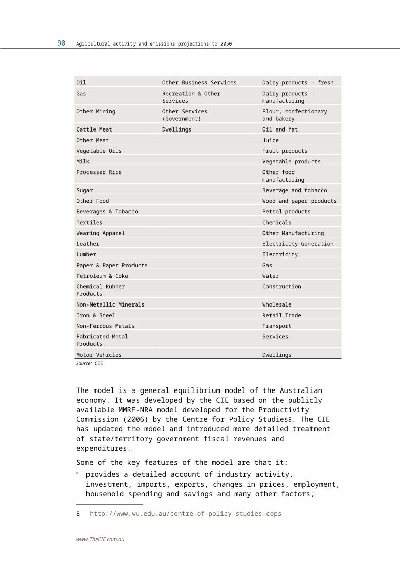
92 Agricultural activity and emissions projections to 2050
‘elasticity’, describing the percentage change in one variable (demand, for example) in response to a one per cent change in another variable (price, for example).The approach to deriving parameter values varies, depending on the nature of the parameter and the information sources available. Deriving parameter values is based around the following sets of alternatives.■ Econometric (statistical) estimation using historical data. This is the
approach taken, for example, in deriving the income and price elasticities of demand within the GMI model (in this case, estimation was based around an Almost Ideal Demand System).
■ Drawing on parameter estimates from published literature. Within agricultural economics there is a long history of statistically estimating and publishing a range of ‘elasticities’ including demand and supply elasticities. Drawing on published literature is the approach taken for some of the supply parameters within the grain and dairy models. Here we include parameters taken from the Global Trade Analysis Project (GTAP).
■ Drawing on specific industry expertise, including industry knowledge of cost and production functions. This approach is used for a number of parameters within the GMI model where statistical estimation is not possible. Industry experience contains a rich source of information to help verify economic models.
■ Calibration of model parameters using observed industry responses to particular economic changes. This approach is similar to statistical estimation but is specifically designed to use recent information (rather than a long time series) to ensure that model parameters reproduce observed market behaviour. This is the approach taken to the ‘Armington’ elasticities within the GMI model.
Table summarises the parameters used in each of the three models, while tables to provide values for some of the key model parameters.
A11AModel parameters and their functionsParameters Function within the model
Global Meat Industry (GMI) model
Income elasticity of demand This captures changes in consumer demand for each meat type as income changes. Typically, red meats are ‘income elastic’, meaning that demand is highly responsive to changes in income.
Price elasticity of demand Captures the response of consumers to changes in relative meat prices.
Elasticity of substitution between domestic Captures the extent to which importing
www.TheCIE.com.au

Agricultural activity and emissions projections to 2050 93
and imported products as well as between imported products from different sources (the ‘Armington’ elasticities)
countries respond to relative price changes of products from different origins. Designed to capture the fact that different meat products from different countries have different quality specifications.
Price elasticity of supply The extent to which supply (by country) is able to respond to price changes.
Dairy model
Supply elasticity The extent to which supply (by country) is able to respond to price changes.
Income elasticity of demand This captures changes in consumer demand for each dairy product as income changes. Often, particular dairy products are ‘income elastic’, meaning that demand is highly responsive to changes in income.
Price elasticity of demand and elasticity of demand substitution between dairy products
Captures the response of consumers to changes in relative prices of different dairy products.
Elasticity of substitution between domestic and imported products as well as between imported products from different sources (the ‘Armington’ elasticities)
Captures the extent to which importing countries respond to relative price changes of products from different origins.
Grains model
Income elasticity of demand Captures changes in consumer demand for grain products as income changes.
Price elasticity of demand Captures the response of consumers to changes in relative prices of different dairy products.
Elasticity of substitution between Australian and foreign grains (an ‘Armington’ elasticity).
Captures the extent to which importing countries respond to relative price changes of products from different origins.
Elasticity of transformation from gross grain output to individual grain output — supply elasticity
Captures the extent to which individual grain output changes (given total capacity) in response to relative price changes.
Elasticity of substitution between primary factors in farming and processing
Captures the technical ability to substitute between land, labour and capital in production and in response to relative price changes.
Elasticity of substitution between grain inputs in processing
Captures the ability of the grain processing industry to substitute between different grains in production.
Source: CIE
A11ARange of income elasticities in the GMI modelDeveloping countries Developed countries
Beef 0.8 to 1.0 0 to 0.8Sheep meat 0.5 to 1.0 0 to 0.5Pig meat 0.2 to 1.0 0 to 0.3Poultry 0.5 to 0.9 0 to 0.2Source: CIE GMI model assumptions
www.TheCIE.com.au

94 Agricultural activity and emissions projections to 2050
A11ARange of price elasticities in the GMI modelDemand Supply
Beef -0.8 to -1.4 0.4 to 0.6Sheep meat -0.8 to -2.5 ~0.2Pig meat -0.7 to -2.5 0.2 to 0.7Poultry -0.6 to -0.9 1.0 to 2.0Source: CIE GMI model assumptions
A11AElasticities for dairy productsDeveloping countries Developed countries
Income elasticities of demandFresh and UHT milk 1.00 0Other dairy products 2.00 0Price elasticities of demandFresh and UHT milk -0.15 -0.15Other dairy products -0.25 -0.25Australian price elasticities of supply
Australia
Raw milk 0.50Dairy products 0.63Source: CIE Dairy model assumptions
A11ADemand elasticities for grain productsDeveloping countries Developed countries
Income elasticities 0.6 0.0Price elasticities Export demand for grains -0.5 -0.5 Export demand for processed products and feed
-10.0 -10.0
Domestic demand for processed products and feed
-2.0 -2.0
Source: CIE Grains model assumptions
A11AElasticities of transformation or substitution in the Grains modelParameter Value
Transforming to individual grain output 1.0Substitution between primary factors in grain farming 1.0Substitution between primary factors in processing 0.5Substitution between individual grain in processing 1.0Substitution between Australian and foreign products 10.0
www.TheCIE.com.au

Agricultural activity and emissions projections to 2050 95
Source: CIE Grains model assumptions
www.TheCIE.com.au

96 Agricultural activity and emissions projections to 2050
B Baseline scenario assumptions
Economic growth
Global and Australian economic growthWorld economic growth is a major demand side input into the modelling. The world economic growth assumptions are made outside the formal modelling and based on historical data, International Monetary Fund projections to 2019 (IMF 2014b) and CIE judgement after 2019. Tables and summarise the historical and the latest projections by the IMF of major economies in the world. Historical data is divided into two periods – from 1980 to 2007 and from 2008 to 2012 – to reflect the impact of the global financial crisis (GFC).
B02BB078 Trend historical growth for major global economies1980-2007 2008-2012
%pa %pa
Australia 3.45 2.47China 9.96 9.29India 5.84 7.69United States 3.27 1.28European Union 2.50 0.11Rest of Asia 3.39 2.17Rest of the World 3.72 2.94Source: IMF World Economic Outlook Database, April 2014
It is evident that the economic growth in the United States and European Union plummeted following the GFC, while China’s growth did not change too much due to the massive scale of the stimulus package implemented by the central and local governments in China. The average growth in India after the GFC has been higher than the average growth before. Cushioned by strong demand from China and India, the Australian
www.TheCIE.com.au

Agricultural activity and emissions projections to 2050 97
economy escaped the crisis albeit the average growth rate dropped by about one percentage point.According to the IMF, the EU economy will have a slow recovery with an average annual growth rate of only 1.8 per cent in the next six years. The recovery in the US will be quicker, with an average rate of 2.8 per cent per annum, comparable to the pre-GFC rate of 3.3 per cent.The annual growth rate in China is projected by the IMF to fall by more than two percentage points to 6.9 per cent in the next six years. This reflects the view that the high growth China has managed to achieve for over two decades is not sustainable because it has relied heavily on exports and investment, distorting patterns of domestic consumption and leading to slowing returns. The stimulus package implemented during the GFC might support growth for a short time, but probably just delay the process of correction of long overdue problems.The Department of Environment (DoE) provided the assumed Australian GDP growth rate. Compared to the IMF projections, the DoE series present a quicker recovery after 2016, with a growth rate of 3.6 per cent per annum which is on a par with the pre-GFC growth trend. After five years of constant growth at 3.6 per cent, it is assumed that the growth rate will gradually fall to 2.9 per cent by 2025.For other economies, we make the following assumptions:■ adopt the IMF projection for other countries for the period up to 2019;
and■ gradual convergence to 2.5 per cent growth for all economies over 81
years after 2019.In the long term, a standard economic assumption is that the economic growth rate of each region will converge. A convergence approach is the basis of the assumptions presented here. The rate of 2.5 per cent was used to be consistent with the long term projected growth rate for Australia provided by DoE.Table summarises the assumed economic growth for major global economies. Forecasting economic growth for 37 years is a near impossible task. We rely on the expert judgement of the IMF for the projections to 2019. There is still a significant degree of uncertainty in these relatively short term projections. For example, in its recent July update, the IMF revised its projection of 2014 global economic growth from 3.7 per cent to 3.4 per cent (IMF 2014c).
www.TheCIE.com.au

98 Agricultural activity and emissions projections to 2050
B02BB079 Average rate of assumed global economic growth2013-19 2020-25 2026-40 2041-50
%pa %pa %pa %pa
Australia 3.06 3.20 2.82 2.59China 7.05 6.22 5.41 4.56India 6.10 6.44 5.57 4.67US 2.62 2.23 2.27 2.32European Union 1.52 1.86 1.95 2.06Rest of Asia 2.83 3.02 2.94 2.83Rest of the World 3.08 3.47 3.30 3.10Source: IMF (2014b) for 2013-19; CIE assumptions for 2019-50; DoE for Australian assumptions.
Exchange rate and energy pricesAssumptions for Australia’s exchange rate were provided by the Department of Environment and are assumed to be between 80 and 90 US cents per Australian dollar over the projection period. Agricultural production is sensitive to fuel and energy prices as they represent a high proportion of production inputs. Chart reports the assumed major fuel price indexes provided by DoE. In the modelling undertaken here, the assumed energy price changes shown in chart affect the input costs and relative prices in the Food Processing model and the individual commodity models.
BError! No text of specified style in document.Error! No text of specified style in document.BBError! No text of specified style in document.80 Assumed price indexes of major fuel commodities
0
50
100
150
200
250
2011-12 2015-16 2019-20 2023-24 2027-28 2031-32 2035-36 2039-40 2043-44 2047-48
Index
(201
1-12=
100)
Oil LNG Thermal coal
Data source: DoE
www.TheCIE.com.au

Agricultural activity and emissions projections to 2050 99
Population growthPopulation growth assumptions are drawn from the United Nations Population Division (UNPD 2013) and ABS (2013a).
World population growthChart shows the index of population (with Year 2012 being 100) for the major world economies. They are drawn from the UNPD’s population projection with medium fertility assumption, except for Australia where the projections are from the Series B of ABS population projections.As shown in the chart, Australia has the second highest population growth among the seven country/country groups, only after the rest of the world.It is interesting to note that China’s population will peak around 2030, and by 2052 it will be less than the level in 2012.
BError! No text of specified style in document.Error! No text of specified style in document.BBError! No text of specified style in document.81 Assumed world population growth
Data source: UN Population Division, ABS
Australian population growthAustralian state population growth is drawn from Series B of ABS population projections. Chart shows the assumed increase in population for each state (from a base of 2012).
www.TheCIE.com.au

100 Agricultural activity and emissions projections to 2050
BError! No text of specified style in document.Error! No text of specified style in document.BBError! No text of specified style in document.82 Assumed Australian population growth
Data source: ABS
Trade policyAustralia has recently concluded negotiating free trade agreements (FTA) with Japan and Korea. Seven other FTAs are currently under negotiation. Depending on the details of the agreements, these new and prospective FTAs could potentially have significant implications for the demand of Australian agricultural products – and therefore production.Those sectors with large reductions in Korean tariffs would be expected to see comparatively large increases of exports to Korea (the most significant sectors are dairy and beef). Removal of a tariff barrier leads to the first round impact of decreasing the price paid by importers and increasing the price received by exporters. This acts to increase demand for these products. However, due to the constraints on Australian agricultural production described in the body of the report as represented by the supply elasticities used in the models, Australian farmers are limited in their production response to higher prices. Some increase in production is expected, however, the most significant impact of the FTAs is trade diversion. That is, Australian exports are redirected from other destinations to the FTA partner country. As an illustration of this, under a simulated FTA between Korea and Australia for RIRDC (Tulloh et al 2014), removal of 27 per cent Korean tariffs on Australian beef leads to an increase of exports to Korea of 110 per cent but a decline in exports to other countries. Total exports of beef increase by only 12 per cent and production of beef increases by only 5.1 per cent.
www.TheCIE.com.au

Agricultural activity and emissions projections to 2050 101
The Japan-Australia Economic Partnership Agreement is less comprehensive than the Korea-Australia FTA, however, it is still expected to feature lower tariff barriers to the Japanese market for Australian agricultural producers including dairy and meat products.
Implications of assumptionsBox provides a description of how changes in the mining sector are affecting agriculture and provides a tangible example of some of the implications the assumptions used may have on the results for the agriculture sector.
B22BB283 Mining slowdown and agriculture
Australia has experienced a mining boom for more than a decade which has resulted in higher income, higher Australian dollar, and higher costs especially labour and material costs.It is commonly held that the mining boom is over as evidenced by slower growth or even falling commodity prices. This will have impacts on the agricultural industry, both positive and negative.Slower growth in the mining sector will reduce the demand for various inputs such as labour, capital and machinery, and materials, mitigating the pressure on prices of these inputs. As a result, agriculture is likely to benefit from this slowdown of mining activity because the costs of inputs will be lower or the growth in costs slower.Slowing down of mining industry in Australia is likely to see a depreciation of the Australian dollar, which will improve the competitiveness of Australian agricultural products and thus help the exports of these products. It is projected that the Australian dollar will depreciate by about 16 per cent by the end of 2020s.At the same time, however, a slowdown in the mining sector means slower growth in income in Australia. Moreover, slowing down of the mining industry in Australia is also a sign of a slowdown of economic activities overseas. Slower income growth will, in turn, reduce the demand for agricultural products. This adverse impact of lower income growth on demand is generally small for a developed country like Australia. However, it will have more severe impact on demand from developing countries. For example, meat products in general have higher income elasticity for relatively lower income households, that is, lower income will result in bigger adverse impact on meat demand.
www.TheCIE.com.au

102 Agricultural activity and emissions projections to 2050
Commodity specific assumptions
MeatChart shows the average slaughtering weight index for meat animals, and chart the index of ratio of slaughtered to total animal numbers. In general the average slaughtering weight has been growing. On the other hand, the ratio of slaughtered to total sheep numbers has been rising although with fluctuation, while the ratio for beef cattle has been falling. This ratio is primarily determined by whether farmers are destocking or rebuilding herds and flocks. In the long term, with an assumed return to average seasonal conditions, the ratio of slaughtered to total animal numbers would be expected to remain constant.
BError! No text of specified style in document.Error! No text of specified style in document.BBError! No text of specified style in document.84 Average slaughtering weight
50
60
70
80
90
100
110
1967 1970 1973 1976 1979 1982 1985 1988 1991 1994 1997 2000 2003 2006 2009 2012
Index
, 201
2=00
Beef and veal
Mutton
Lamb
Pig
Chicken
Data source: ABARES Australian Commodity Statistics 2013
www.TheCIE.com.au

Agricultural activity and emissions projections to 2050 103
BError! No text of specified style in document.Error! No text of specified style in document.BBError! No text of specified style in document.85 The ratio of slaughtered to animal numbers
50
60
70
80
90
100
110
120
1991 1993 1995 1997 1999 2001 2003 2005 2007 2009 2011
Index
, 201
2=10
0
Beef cattle
Sheep
Data source: ABARES Australian Commodity Statistics 2013
Tables and summarise the assumed growth in slaughtering weight and the ratio of animals slaughtered to total animal numbers, respectively, for the GMI model. They are key parameters to translate the projected meat production to animal numbers.
www.TheCIE.com.au
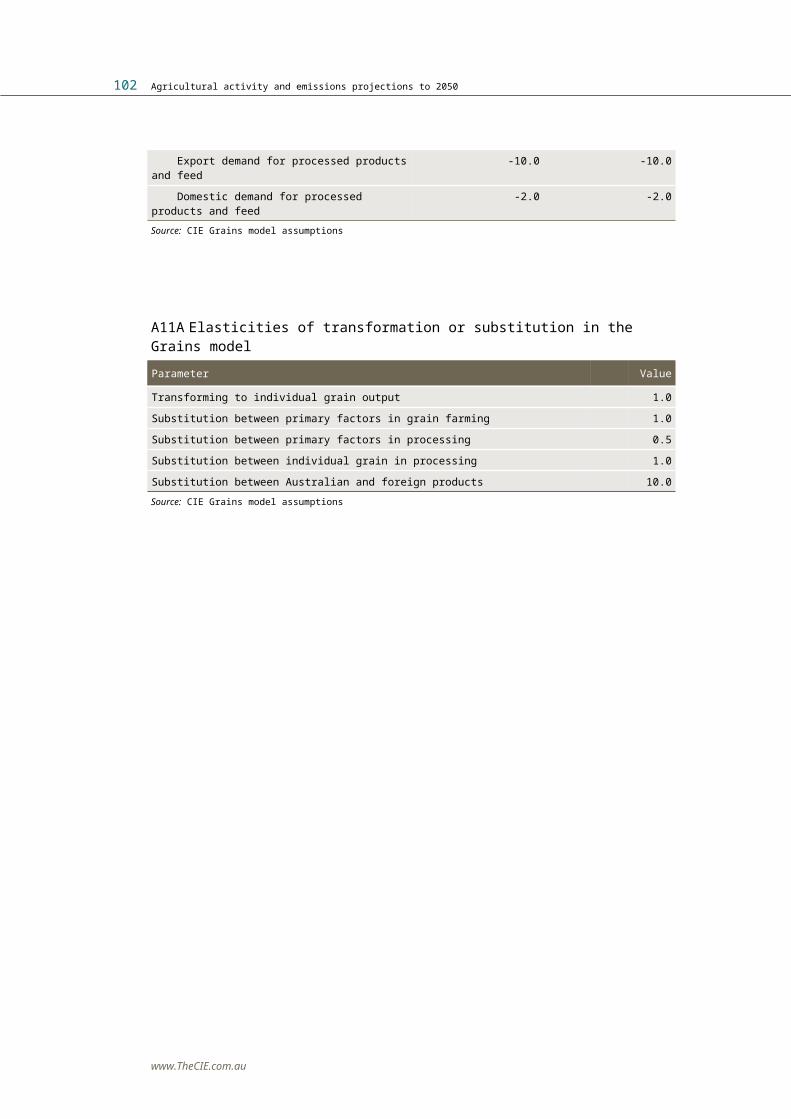
104 Agricultural activity and emissions projections to 2050
B02BB086 Assumed growth in slaughtering weight: GMI modelBeef and veal Mutton Lamb Pigs Poultry
2014 -2.01 1.26 0.09 0.44 0.892015 1.66 0.18 0.39 0.68 0.892016 -0.98 0.26 -0.20 -0.80 0.892017 0.29 -0.67 -0.46 -0.17 0.892018 -0.11 0.01 0.47 -0.18 0.892019 -1.12 0.00 0.01 -0.20 0.892020 0.21 0.38 -0.15 0.34 0.892021-30 0.65 0.95 0.26 0.40 0.892031-40 0.52 0.76 0.21 0.32 0.712040-50 0.42 0.61 0.17 0.26 0.57Source: Historical and industry data, CIE assumptions
B02BB087 Assumed growth in the ratio of slaughtered to animal numbers: GMI model
Beef and veal Mutton Lamb Pigs Poultry
2014 20.06 15.79 15.79 0.00 0.002015 -2.93 -11.14 -11.14 0.00 0.002016 -8.34 -4.89 -4.89 0.00 0.002017 -2.77 0.15 0.15 0.00 0.002018 2.82 -0.88 -0.88 0.00 0.002019 2.76 -2.26 -2.26 0.00 0.002020-30 0.10 0.12 0.12 0.00 0.002031-40 0.01 0.01 0.01 0.00 0.002040-50 0.00 0.00 0.00 0.00 0.00Source: Historical and industry data, CIE assumptions
Table summarises the long term productivity assumptions for meat commodities and country groups identified in the GMI model. These were formed from discussions with industry experts.9 Broadly, the pattern of productivity changes evident in table B.12 reflects the stage of development of the various meat industries in the countries covered. In general, the US has the highest productivity growth in most cases to which other countries are generally converging. In particular:■ in grass and grain fed beef, the Latin American countries have the
highest productivity growth rates as these countries are adopting US technologies and are in a catch up and expansion phase, including increases in scale that allow higher productivity growth. In contrast, most of the Asian countries (with the exception of India) have
9 The CIE has ongoing engagement with the meat industry and it is based on these interactions that the views on industry productivity are based.
www.TheCIE.com.au
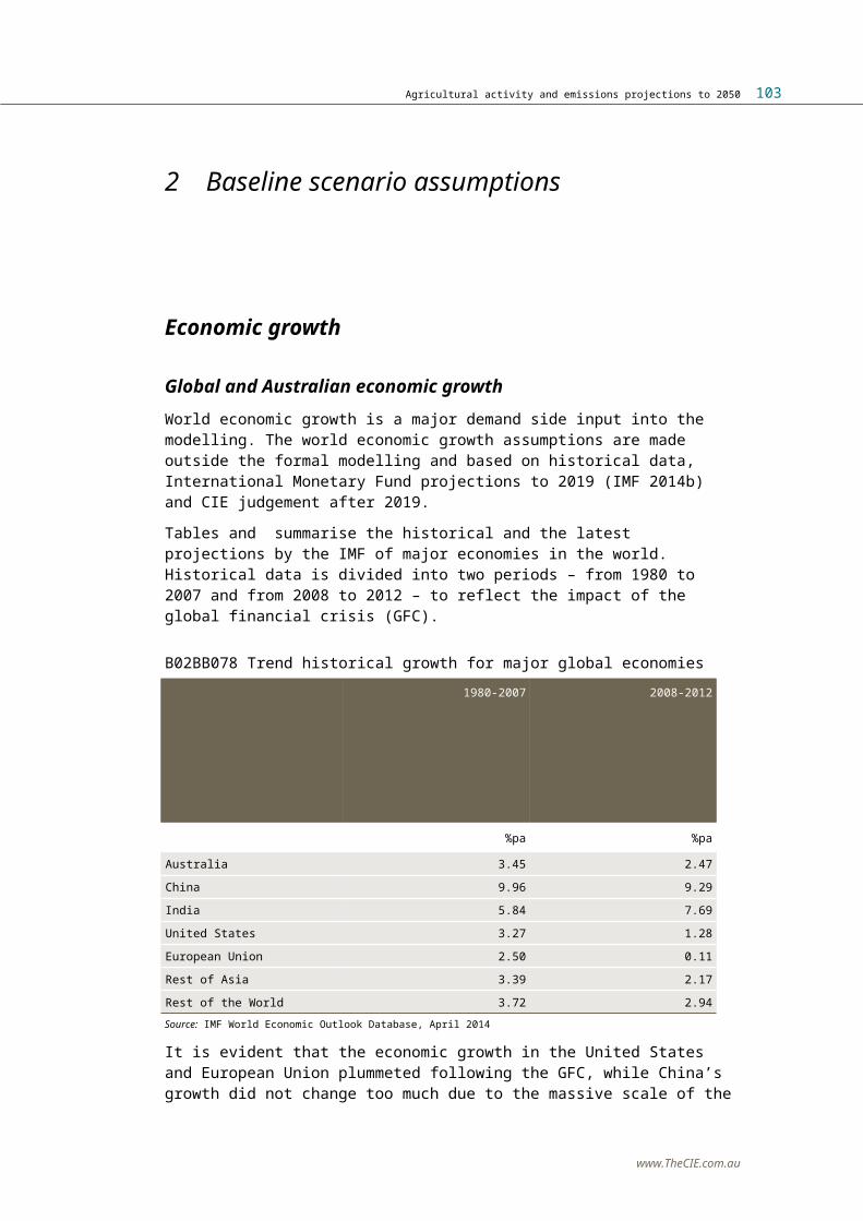
Agricultural activity and emissions projections to 2050 105
considerably less potential to increase productivity in their beef systems.
■ diaphragm beef is a special category capture in the GMI model and has no projected productivity growth independent of its grass or grain fed origins.
■ live cattle is a category only relevant to Australia in the GMI model, and is assumed t have the same productivity growth as for grass fed beef.
■ in lamb and sheep meat, both New Zealand and the United States are projected to experience negative productivity growth because of strong competition with other land uses leading to cost pressures and expected declines in lamb and sheep meat production growth rate.
■ also in lamb, the Latin American countries are expected to have high productivity growth rates for the same reason as in the case of beef. In contrast, most of the Asian economies have limited potential for increased productivity in lamb and sheep based systems, so the projected productivity growth rates are lower.
■ in pig meat and poultry production, the Asian economies are generally projected to have higher productivity gains as they are steadily moving from smallholder to more intensive production systems which will leader to higher productivity growth than countries where this transition has mostly already occurred.
■ in seafood, the only projected productivity gains are in the Asian economies, due largely to the expected implementation of large scale aquaculture systems.
■ most wool producing economies are expected to have low (or zero) productivity growth reflecting limited potential for productivity growth in wool production. One of the lowest wool productivity growth rates is in Australia. This largely reflects competition with sheep based meat products which are in most cases a substitute for wool production.
B02BB088Long term productivity growth for meat commoditiesRegion
Grass fed beef
Grain fed beef
Diaphragm beef
Live cattle Lamb Sheep meat
Pig meat Poultry
% % % % % % %Australia 0.75 0.38 0.00 0.75 0.38 0.00 0.75 1.00New Zealand 0.50 0.00 0.00 0.00 -1.00 -1.00 0.50 1.00United States 0.75 1.00 0.00 0.00 -2.00 -2.00 0.75 1.00Canada 0.75 1.00 0.00 0.00 0.50 0.00 0.75 1.00Japan 0.00 0.00 0.00 0.00 0.00 0.00 0.00 0.00South Korea 0.00 1.50 0.00 0.00 0.33 0.00 0.50 0.50Taiwan 0.66 0.00 0.00 0.00 0.33 0.00 0.00 1.00
www.TheCIE.com.au

106 Agricultural activity and emissions projections to 2050
Hong Kong 0.10 0.00 0.00 0.00 0.33 0.00 1.00 1.00Singapore 0.10 0.00 0.00 0.00 0.33 0.00 1.00 1.00Malaysia 0.10 0.00 0.00 0.00 0.33 0.00 1.00 1.00Indonesia 0.00 0.00 0.00 0.00 0.33 0.00 1.00 1.00Thailand 0.10 0.00 0.00 0.00 0.33 0.00 1.00 1.00Philippines 0.10 0.00 0.00 0.00 0.33 0.00 1.00 1.00China 0.20 0.00 0.00 0.00 0.33 0.00 1.00 1.00European Union 0.50 0.00 0.00 0.00 0.00 0.00 0.50 0.50Mexico 1.22 0.00 0.00 0.00 1.00 0.00 0.75 1.00Argentina 1.22 1.44 0.00 0.00 1.00 0.00 0.75 1.00Uruguay 1.22 1.44 0.00 0.00 1.00 0.00 0.75 1.00Paraguay 1.22 1.44 0.00 0.00 1.00 0.00 0.75 1.00Brazil 1.50 1.44 0.00 0.00 1.00 0.00 0.75 1.00India 2.00 0.00 0.00 0.00 1.00 0.00 1.00 1.00Russian Federation 0.10 0.00 0.00 0.00 0.00 0.00 0.75 1.00Other countries 0.10 0.00 0.00 0.00 0.33 0.00 1.00 1.00Source: CIE assumptions
www.TheCIE.com.au
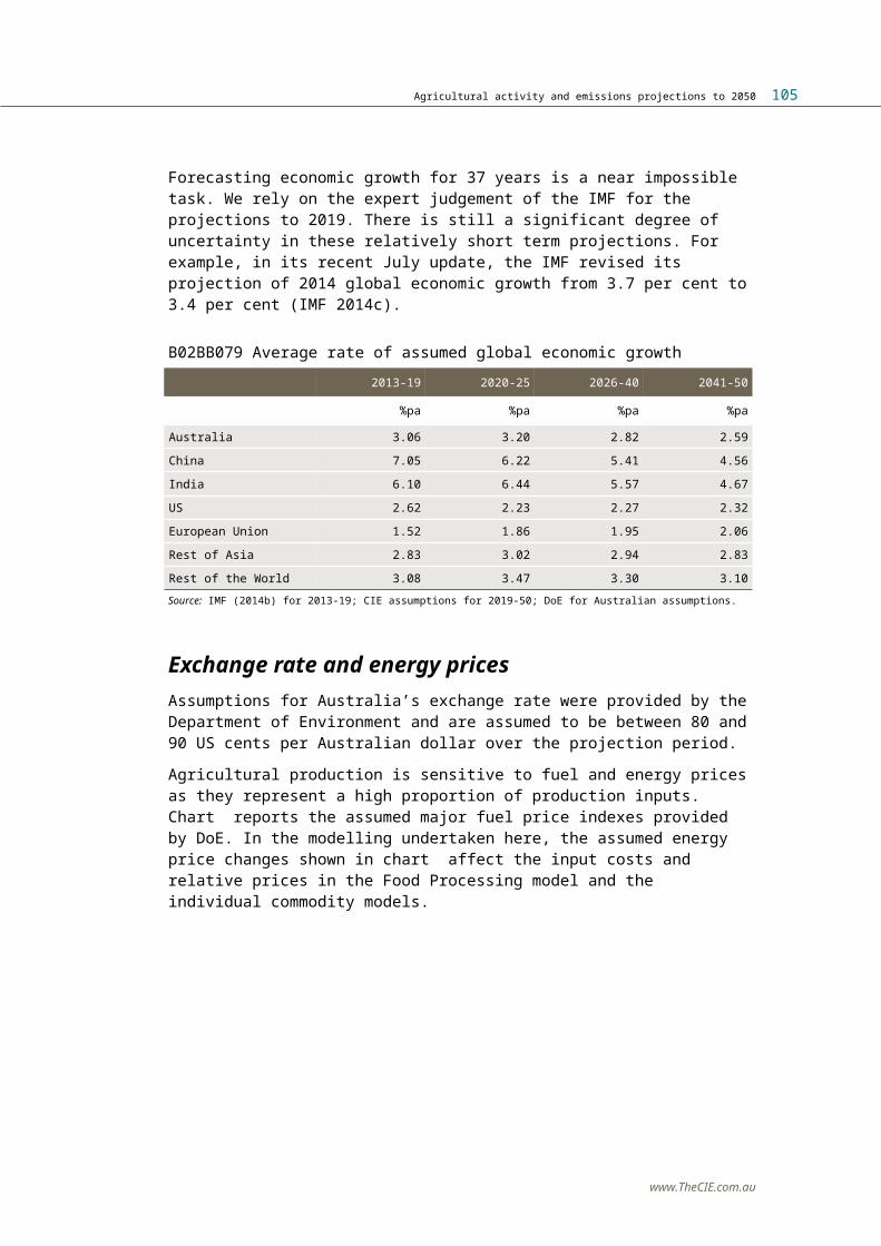
Agricultural activity and emissions projections to 2050 107
DairyChart shows the milk yield per cow and the ratio of cow numbers to cattle numbers in Australia. It appears that the yield has been steadily growing in the past, although with some fluctuations. On the other hand, the cow to cattle ratio has been falling, most notably since the late 1990s. This fall can be explained by recent changes in the fertility of the dairy herd. Without any basis for assumptions to the contrary, the ratio of cows to cattle is assumed to remain constant over the projection period.Table sets our assumptions for the dairy model. These assumptions are based on historical observations and discussions with industry experts.
BError! No text of specified style in document.Error! No text of specified style in document.BBError! No text of specified style in document.89 Milk yield per cow and ratio of cow number to cattle number
1967-68
1968–69
1969–70
1970–71
1971–72
1972–73
1973–74
1974–75
1975–76
1976–77
1977–78
1978–79
1979–80
1980–81
1981–82
1982–83
1983–84
1984–85
1985–86
1986–87
1987–88
1988–89
1989–90
1990–91
1991–92
1992–93
1993–94
1994–95
1995–96
1996–97
1997–98
1998–99
1999–2000
2000–01
2001–02
2002–03
2003–04
2004–05
2005–06
2006–07
2007–08
2008–09
2009–10
2010–11
2011–12
2012–13
0
1000
2000
3000
4000
5000
6000
7000
0.00
0.10
0.20
0.30
0.40
0.50
0.60
0.70
0.80
Yield (LHS)Cow to cattle ratio (RHS)
Yiel
d
Data source: ABARES Australian Commodity Statistics 2013
B02BB090 Productivity improvement growth rate assumptions: the Dairy model
2013-20 2020-30 2030-40 2040-50
Milk production per cow in Australia % 1.5 1.3 0.8 0.5 Ratio of cow number to cattle number
% 0.0 0.0 0.0 0.0
Input efficiencyAustralia % 1.5 1.5 1.5 1.5 New Zealand % 1.5 1.5 1.5 1.5 European Union % 0.0 0.0 0.0 0.0
www.TheCIE.com.au

108 Agricultural activity and emissions projections to 2050
United States % 0.5 0.5 0.5 0.5 Rest of the world % 1.0 1.0 1.0 1.0 Source: CIE assumptions.
GrainsTotal factor productivity growth in cropping (the whole grains sector) has tended to vary considerably from year to year, although there is some evidence that this has been slowing. For example, between 1978 and 1988 average productivity growth was 3.2 per cent a year. For the period 1989 to 1999 this had slowed to 1 per cent a year, and for 2000 to 2011, this slowed again to 0.3 per cent a year (see Dahl, Leith and Gray 2013).The projections presented here assume that long term total factor productivity in the grains industries returns to 0.6 per cent a year, lower than the long term average but higher than the most recent experience.
www.TheCIE.com.au

110 Agricultural activity and emissions projections to 2050
www.TheCIE.com.au
THE CENTRE FOR INTERNATIONAL ECONOMICSwww.TheCIE.com.au