WORKING PAPERAGRICULTURAL PRODUCTIVITY AND DEFORESTATION IN BRAZIL

JULIANO ASSUNÇÃOAHMED MUSHFIQ MOBARAKMOLLY LIPSCOMBDIMITRI SZERMAN

DECEMBER 2016

THEME

AGRICULTURE, ENVIRONMENTAL PROTECTION

KEYWORDS

ELECTRICITY, HYDRO-POWER, AGRICULTURE, PRODUCTIVITY, DEFORESTATION, BRAZIL

The Land Use Initiative (INPUT – Iniciativa para o Uso da Terra) is a dedicated team of specialists who work at the forefront of how to increase environmental protection and food production. INPUT engages stakeholders in Brazil’s public and private sec¬tors and maps the challenges for a better management of its natural resources. Research conducted under INPUT is generously sup¬ported by the Children’s Investment Fund Foundation (CIFF) through a grant to the Climate Policy Initiative. www.inputbrasil.org

Agricultural Productivity and Deforestation inBrazil

Juliano Assunção

PUC-Rio

Molly Lipscomb

University of Virginia

Ahmed Mushfiq Mobarak

Yale University

Dimitri Szerman

PUC-Rio

December 13, 2016

[PRELIMINARY AND INCOMPLETE.]Click here for the latest version.

Abstract

When deforestation laws are difficult to enforce, increased agricultural pro-

ductivity and intensification are used as an indirect policy tools to reduce the

pressure to clear forests for new land, a strategy known as the “Borlaug hypoth-

esis”. Increasing productivity can have ambiguous effects on forest protection

in theory: it can expand the scope of farming, which is detrimental to the for-

est, but it can also induce farmers facing factor-market constraints to shift away

from land-intensive cattle grazing toward less-harmful crop cultivation. We ex-

amine these predictions using five waves of the Brazil Agricultural census, 1970

- 2006. We identify productivity shocks using the expansion of rural electrifi-

cation in Brazil during 1960-2000. We show that electrification increased crop

productivity, and farmers subsequently both expand farming through frontier

land conversion, but also shift away from cattle ranching and into crop culti-

vation. The latter allows farmers to retain more native vegetation within rural

settlements. Overall, electrification causes a net decrease in deforestation. We

also show that Brazilian farmers are credit constrained and invest more in capi-

tal following electrification, consistent with the theory we build. We address the

endogeneity of electrification by developing a model that forecasts hydropower

dam placement based on topographic attributes of each location, and isolate the

exogenous portion of the panel variation in electrification.

Keywords: Electricity, Hydro-power, Agriculture, Productivity, Deforestation, Brazil

1

1 Introduction

The rapid loss of major tropical forest ecosystems has been one of the major envi-ronmental disasters of the last century. Nearly 20% of recent global greenhouse gasemissions are attributed to tropical deforestation (Stern, 2008). The vast biodiversityacross large, diverse ecological zones of Brazil, along with the agricultural potentialthat land represents, makes the country singularly important in the tension betweendevelopment and environmental sustainability. While there has been a decelerationin the rate of deforestation in Brazil recently, 78,564 square kilometers of forest coverwas lost in the last seven years, and the scale of the problem therefore remains enor-mous (MMA, 2013).

Deforestation is intricately tied to decisions on land use for agricultural production. 1

Agricultural productivity in frontier areas, and land intensity of the type of farmingthat gets practiced – crop cultivation versus cattle grazing – are the key determinantsof deforestation. Brazil produces over a hundred billion dollars annually throughlarge-scale crop cultivation, and ranks among the world’s three largest producersof sugarcane, soybeans and maize. Crop output increased 365% between 1996 and2006, and Brazil has been dubbed “the farm that feeds the world” (The Economist,August 26, 2010). Brazil is also the world’s largest exporter of beef, with a ten-foldincrease in exports during that decade. Many farmers engage in both cultivation andcattle-grazing simultaneously.

Cattle grazing and crop cultivation pose very different risks for deforestation, andthis margin of land use decisions will be central to our analysis. Cattle grazing isextremely land intensive with limited use of confinement in Brazil, and the aver-age stocking ratio reported in the 2006 agricultural census was less than 1 head perhectare. In contrast, crop cultivation accounted for only 10.6% of total farm area, but60% of the value of output in 2006 (IBGE). Increasing crop productivity can thereforehave ambiguous effects on deforestation in theory. It has the potential to curb defor-estation by inducing land conversion away from grazing and into more intensivecropping, but it could also induce expansion of agriculture into frontier lands.

This paper starts by developing a framework that allows for both the intensificationeffect (Borlaug’s hypothesis) as well as the expansion effect. In our model, farmersengage in two activities that are different with respect to their factor intensities –we label the more land-intensive activity “cattle grazing” and the capital-intensive

1While logging is often the proximate cause of land clearing, re-growth occurs in most moisttropical forests. For areas to remain deforested in the longer term, the propensity to convert the landto agricultural use matters most.

2

activity “crop cultivation”. The farmer faces a factor market constraint that limitsgrowth. Any productivity shock biased towards cropping will induce farmers toswitch into cultivation and decrease the land allocation to grazing. The shift awayfrom the activity that is more land intensive decreases overall land use, and bene-fits native vegetation. On the extensive margin, increased agricultural productivityinduces new people to move into farming, which has the opposite effect on defor-estation. The overall effect on deforestation is therefore theoretically ambiguous, andthis motivates our empirical inquiry.

The empirical exercise uses the impressive expansion of the electricity grid in Brazilduring the period 1960-2000 that electrified many frontier areas and farms as a mea-sure of a shock to agricultural productivity. Using county-level data, we first docu-ment that electricity access increases cropping productivity more than cattle grazingproductivity. Next, we show that farmers (i) allocate less land to pastures, (ii) leavemore land in native vegetation, and (iii) invest in more capital following an increasein electricity infrastructure. Although cropland as fraction of total farmland remainsunchanged, farmers substitute subsistence varieties for the ones that benefit mostfrom electricity. Finally, we find weak evidence that the increase in agricultural pro-ductivity leads to an expansion in farming and induces frontier land conversion.Overall, our empirical results are consistent with our framework, and suggest thatelectrification causes a net decrease in deforestation in Brazil.

To address the endogeneity issues inherent in infrastructure data (where investmentmay follow demand), we use the IV estimation strategy developed in Lipscombet al. (2013). We forecast hydropower dam placement and transmission grid ex-pansion based on exogenous topographic attributes of each location. The forecast-ing model produces hypothetical maps that show, given the constrained budget ofgeneration plants for each decade, how the electrical grid would have evolved hadinfrastructure allocation been based solely on cost considerations, ignoring demand-side concerns. The maps isolate the portion of the panel variation in electricity gridexpansion that is attributable to engineering cost considerations, and thereby pro-vide exogenous variation in electricity access which we use as an instrument foractual electrification. Our empirical strategy takes advantage of the fact that Brazilrelies almost exclusively on hydropower to meet its electricity needs. The cost of hy-dropower dam construction depends on topographic factors such as water flow andriver gradient, since hydropower generation requires intercepting large amounts ofwater at high velocity. The forecasting model includes location fixed effects to con-trol for the fixed geographic attributes, so that the identification comes only fromdiscontinuities in the ranking of different locations’ suitability for dam construction,

3

given the decade-specific budget constraints.

An assumption underlying strategies aimed at reducing deforestation through in-creased investment in capital for rural farms is that increased productivity will leadto agricultural intensification which reduces the pressure to clear forests for newland, rather than expand the scope of farming. Our model indicates that this a po-tentially dangerous strategy, because it has ambiguous effects on land use in theory.Our empirical results indicate that productivity-enhancing strategies did allow fordecreased net deforestation in Brazil over the period 1970-2000. Improvements inagricultural productivity appear to be a promising avenue for environmental protec-tion when regulators’ capacity to enforce forest protection laws is weak. Our analysissuggests that the net effect on deforestation will depend on the type of activity thatgets displaced when agriculture becomes more productive. In Brazil, the prolifer-ation of land-intensive cattle grazing makes improved cultivation beneficial for theenvironment.

The beneficial environmental effect of the expansion in electricity infrastructure standsin contrast to Pfaff (1999), Cropper et al. (1999) and Cropper et al. (2001), who showthat road infrastructure aids deforestation in Brazil and Thailand, respectively. Stavinsand Jaffe (1990) find that flood-control infrastructure projects account for 30 percentof forested wetland depletion in the Mississippi Valley by affecting private land usedecisions. Our nuanced findings on the opposing effects of infrastructure develop-ment on deforestation contribute to a long-standing literature on the non-monotonicrelationship, also known as the Environmental Kuznets Curve (EKC), between eco-nomic growth and environmental outcomes, starting with Grossman and Krueger(1991, 1995). The existing empirical evidence on the EKC is mixed and mostly basedon cross-country regressions, see Foster and Rosenzweig (2003) and Cropper andGriffiths (1994).

Our paper is also related to the literature on technology adoption in agriculture(BenYishay and Mobarak, 2014), (Conley and Udry, 2010). It is most closely relatedto papers on causes and consequences of irrigation technology in the United States(Hornbeck and Keskin, 2014) and in India (Sekhri, 2011). We also contribute to arapidly growing literature on the effects of electrification (Dinkelman, 2011; Rud,2012; Lipscomb et al., 2013)) and other forms of infrastructure (Duflo and Pande,2007; Donaldson, ming) on development.

The paper is organized as follows: section 2 discusses historical land use in Brazil,the vast growth in the electricity network during the period 1960-2000, and the ex-pansion of the use of irrigation. Section 3 discusses a simple theoretical model which

4

we use to investigate the contrasting impacts of increased agricultural productivityon land use: the increased intensity of agricultural productivity, versus the poten-tial for expansion across increased land area as agriculture becomes more profitable.Section 4 discusses the three key datasets that we use–the Census of Agriculture inBrazil, Electricity Data from various historical archives in Brazil and elevation mapsfrom USGS, and rainfall data. Section 5 discusses our estimation strategy and the in-strumental variable technique we employ. Section 6 discusses the empirical results,and section 7 concludes.

5

2 Background

Large scale deforestation in Brazil has resulted in a 19% decrease in forest cover in theAmazon since 1970 . This deforestation was, in large part, a result of the widespreadexpansion of agriculture . The conflict between the forest and agricultural land usesis particularly pronounced in areas of Brazil with lower distances and transport coststo major markets: Northern Brazil, the Pantanal and the Cerrado (citation?). This ex-pansion in farmland has occurred at the same time as a widespread increase in farmproductivity stemming from improved seed varieties, improved farming techniques,and increased use of capital in farming. In this section, we discuss the increase inproductivity in the agricultural sector and the reallocation in land use in farmingthat has occurred over the past 50 years.

2.1 The Increase in Agricultural Productivity in Brazil

Agricultural productivity in Brazil has increased significantly since 1970, as Brazilcloses the gap between agricultural productivity in Brazil and the US (Viera Filhoand Fornazier, 2016). This increase in productivity has depended in large part on theability of farmers to invest in new farming technology, and has varied substantiallyacross regions of Brazil (Viera Filho Santos and Fornazier, 2013).

Constraints in Factor Markets The ability to take advantage of productivity im-provements through new technologies is often dependent on the ability of farmers toinvest in new capital equipment and to hire workers with higher levels of educationthan traditional farm labor. One common feature of rural economies in developingcountries is presence of frictions, and ensuing constraints faced by producers in fac-tor markets (Conning and Udry, 2007). For example, between 1960 and 2006 at least80 percent of Brazilian farmers had no access to external financing of any sort. Farm-ers who did obtain credit typically used it for short-term loans to finance materials —seeds, fertilizer and pesticides — or transportation, as opposed to long-term invest-ments. Access to other financial products, such as insurance, is even less commoneven today. Agricultural labor markets in general, and in developing economies inparticular, are also plagued by informational frictions and strict regulations whichcreate constraints for producers to hire labor. In Brazil, these problems have beencompounded by a massive rural-urban migration which decreased labor supply inrural labor markets: the fraction of the population living in rural areas decreasedfrom 64 percent in 1950 to 19 percent in 2000.

6

Electricity and Agricultural Productivity Many of the new technologies for irri-gation and storage of farm production require the use of electricity. In 2006, onein five Brazilian farmers reported using electricity in their production. Farmers useelectricity for various purposes in their agricultural production function. One im-portant use is irrigation. There are two main types of irrigation systems used inBrazil. Flooding or furrow irrigation typically uses gravity to channel water from asource located at higher altitudes than the field. This is a traditional, labor and water-intensive method used for flooding of lowlands in the South for rice production inthe summer since the 1960s. In contrast, sprinkler irrigation systems require energyto lift groundwater and distributed it. Although diesel can be used to provide en-ergy for pumps, using electricity is cheaper not only because of the equipment, butalso because of fuel costs. This was particularly true after the oil price shocks in 1973and 1979, and the expansion of the electricity grid providing cheap energy from hy-dropower (World Bank, 1990; Rud, 2012). Sprinkler systems has been the preferredmethod for crops other than rice in the Center-West, Southeast and Northeast partsof the country. Specially in the Center-West, irrigation during the dry winters al-low for two, and sometimes even three harvests of grains (soybeans, maize, cotton)per growing season, therefore significantly increasing farms’ production value perhectare of land.

Electricity also enables farmers to adopt various technologies to process their out-put. For example, post-harvest handling of grains require an array of machinery fordrying grains, including ventilators and conveyor belts, for which electricity is animportant input. Drying grains is important as it enables producers to store theiroutput and sell it when market prices are good, besides adding value to the output.Livestock production can also benefit from electricity through mechanized milking,pasteurizing and cooling of dairy products, and poultry and egg production.

2.2 Evolution of Land Use in Brazilian Farms

Land use trends over the second half of the twentieth century in Brazil are shownin figure 1, based on data from the Census of Agriculture, described in more detailin section IV. Farmland expanded considerably, reaching 44 percent of the country’sterritory in 1985, from 29 percent in 1960, a 50 percent increase within 25 years, be-fore it started slowly decreasing. Brazilian farmers allocate their land between threemain land use categories—pastureland, cropland and native vegetation . At anypoint in time between 1960 and 2006, these three categories accounted for 80-90 per-cent of total farmland . As can be seen, there were major changes in the allocation

7

of farmland between these three categories over this period. The share of pasture-land, which is almost entirely used for cattle grazing, decreased from a peak of 52percent in 1970 to 48 percent of total farmland in 2006, while the shares of croplandand native vegetation increased from about 9 and 19 percent to 14 and 29 percent, re-spectively.2 These trends show a clear expansion of cropland and native vegetationwithin farmland, at the cost of pastureland and other uses.

Native Vegetation in Private Properties Native vegetation is an important compo-nent of our analysis and forms a large component of land use in Brazilian farms. 3

There are potentially many reasons why producers may decide to keep trees in theirproperties. Although land is a relatively abundant factor in Brazil, land markets areplagued with frictions, from weak property rights to regulations in rental markets.As a result, producers may leave uncultivated land for the sheer reason of not beingable to hire enough labor and capital, nor being able to sell or rent their land. Sec-ond, there are regulations mandating property owners to keep trees in a fraction oftheir land at least since 1934.4 This sort of legislation however can hardly explainthe observed patterns for the period we analyze, as its monitoring and enforcementhas been an historical challenge in Brazil in general, and in rural areas of the coun-try in particular. Illegal deforestation in the Amazon for example only started tobe more seriously tackled with command-and-control policies after peaking in 2004,therefore at the very end of our sample period. Third, agro-forestry production isa source of income and livelihood, specially for smallholders. Although this canpartially explain the presence of native vegetation in farmland, it cannot explain theincrease of native vegetation in farmland at the aggregate level. Over this period,Brazil’s agriculture became increasingly professional, focused on commodities andexport-oriented; the fact that Brazil became the world’s largest soybean producerand exporter is the quintessential example of this trend. Given the increased impor-tance of export-oriented commodities, one would have expected the relative shareof forestry production, and therefore of land allocated to forests in farmland, to de-

2Not surprisingly, these changes mirror changes in productivity (or yield) gains: whereas grossyields in agriculture have quadrupled over the 1970-2006 period, cattle grazing yields, measured asheads per hectare, only doubled.

3The presence of trees among agricultural land is a common feature in the tropics, and not specificto Brazil. Zomer et al. (2014) find that 92 (50) percent of agricultural land in Central America had atleast 10 (30) percent of tree cover in year 2000.

4This legislation, known as the Brazilian Forest Code, was enacted in 1934 and mandated thatevery rural property to keep at least 25 percent of its area in native vegetation, in order to guarantee astock of wood fuel. The Forest Code was amended in 1965 and then in 2012 after long public debates.Enforcement of the Forest Code is only now being taken seriously with the help of high-resolutionsatellite technology, unavailable even in the early 2000’s.

8

crease during this period. Finally, it is possible that producers realize the productionbenefits of having biodiversity in their land, but this is a possibility that we cannottest with our data.

Crops vs Cattle Grazing As practiced in Brazil, cattle gazing and crop cultivationmix inputs at very different rates. Specifically, cattle grazing is a relatively land-intensive activity, whereas crop cultivation requires more capital, both physical andhuman. For example, in 2006 the value of machinery and equipment per hectare inthe typical livestock farm was one-sixth of that of a typical crop farm. And althoughan equal fraction of farms within each activity make investments in machinery andequipment, investment per farm is also lower in livestock farms. These figures arenot surprising when one notes that only 4 percent of cattle farms uses confinement,and that only 0.2 percent of producers pasteurize the milk they sell; and that at thesame time, over 60 percent of the harvested area of maize and sugar cane is mech-anized, as is virtually all of the soybean production in the country. Moreover, cropcultivation demands more human skills than cattle grazing as practiced in Brazil,requiring experimentation with techniques and inputs, such as seeds and fertilizers.In short, the typical cattle grazing farm requires low levels of capital investmentswithin farm gate when compared to crop farming, a fact that motivates some as-sumptions in the model we present in Section 3.

9

3 Conceptual Framework

In this section we build a simple theoretical framework inspired by the salient fea-tures of farming and land use in Brazil, with the goal of generating predictions onhow a productivity shock in crop cultivation will affect farming choices and defor-estation. To mirror the language in our empirical exercise, we refer to the key pro-ductivity parameter in our model as “availability of electricity”, which is denoted byΩ. Our model allows farmers to engage in both crop cultivation and cattle grazingbecause these are the two major categories of agricultural activities, as indicated inthe previous section and in the agricultural census data.

The economy is endowed with total land of H which is initially completely coveredby native vegetation. A continuum of individuals reside in this economy, and eachdecides whether to become a farmer and convert land to agricultural use. Theseagents only differ by their outside option θ, which is their individual-specific oppor-tunity cost of operating a farm. θ ∼ Γ, with pdf γ. The opportunity cost of farmingcan be thought of as the wage rate in the non-agricultural sector, which may increasewith the availability of electricity, and so we allow Ω to shift the distribution of out-side options in the sense of first-order stochastic dominance: Γ(θ; Ω) ≤ Γ(θ; Ω), forall Ω > Ω. The profit from farming activities is common across farmers and is de-noted Π, and the set of farmers is therefore Γ(θ), where θ = θ : θ ≤ Π.

Each farm is a tract of land of size H, which is fully covered by native vegetationbefore farming activities commence. Each farmer can engage in both crop cultivationand cattle grazing, and the areas allocated to each type of activity are denoted Hc andHg, respectively. We assume that the production functions for the two activities aresimilar, except that there is a factor other than land which is more useful in cropcultivation, which we will denote N. Electrification improves the productivity ofN. We think of N as capital, labor, or a combination of both. Our modeling choicereflects the fact that electrification enhances the productivity of crop cultivation morethan cattle grazing. We assume the following forms for the production functions forcrops and cattle grazing: C = ΩNF(Hc) and G = F(Hg), with FH > 0, FHH < 0 andFH(0) = ∞.5

Land and the factor N can be bought in the market at prices p and r, respectively.Farmers are credit constrained and need to fund their expenditures with capital andland from their own resources, M. We normalize the prices of C and G to 1. Thus,

5The factor Ω only entering the production function for crop but not cattle is merely a model-ing simplification. The results we derive only require that electrification benefits crop cultivationrelatively more.

10

each farmer’s problem can be written as:

maxN,Hc,Hg

Π = ΩNF(Hc) + F(Hg)− rN − p(Hc + Hg) (1)

subject to

rN + p(Hc + Hg) ≤ M, (2)

Hc + Hg ≤ H. (3)

We focus on the case where the resource constraint (eq. 2) is binding, because themajority of farmers in Brazil are small and medium holders who face some factormarket constraints in capital, credit or labor which affects their ability to generateN. Land will therefore not be the limiting factor, and the land constraint (eq. 3) willtypically not bind. This focus reflects reality (farming in Brazil expanded into fron-tier lands that just needed to be cleared and occupied during our period of study),and also makes the model interesting and informative. The credit constraint alwaysbinds because the profit function is linear with respect to N and FH(0) = ∞.

In the Appendix, we show that the optimal land use and production choices forfarmers, H∗c (Ω), H∗g(Ω), N∗(Ω), display the following properties:

∂N∗

∂Ω> 0 (4)

∂H∗c∂Ω≥ 0 (5)

∂H∗g∂Ω

< 0 (6)

∂(H∗c + H∗g)∂Ω

< 0 (7)

The intuition behind equations (4)–(7) is straightforward. Since factor N and landallocated to crop cultivation become more productive with electrification, N and Hc

move in the same direction as Ω in this model, as shown in equations (4) and (5).However, since the credit constraint binds, the farmer can only increase land allo-cated to crop cultivation and/or hire more N in response to an increase in electrifi-cation if she decreases land allocated to cattle grazing (equation 6). The total landdemand for agricultural purposes within the farm, H∗c + H∗g , decreases in responseto increases in electrification (equation 7): as farmers switch away from cattle graz-ing and into crop cultivation, they also spend more money on K and hence must give

11

up more of Hg than they can increase Hc.6

The net effect of electrification on deforestation depends not only on intensive-marginchanges in land demand within each farm, but also on how the productivity shockinduces extensive-margin changes in the decision to enter the agricultural sector. Toanalyze this net effect, we define the total area of native vegetation as the differencebetween the economy’s total land endowment and farmer’s total land demand foragricultural purposes:

Hv = H −∫ θ

−∞(H∗c + H∗g)dΓ(θ) (8)

The derivative of the total area of native vegetation with respect to electrification hastwo effects:

dHv

dΩ= −

d(H∗c + H∗g)dΩ

Γ(θ)︸ ︷︷ ︸>0

− (H∗c + H∗g)Γ(θ)dθ

dΩ︸ ︷︷ ︸≶0

(9)

The first term relates to the intensive-margin adjustment, through which electrifica-tion reduces the land demand for each farmer by inducing farmers to shift away fromland-intensive cattle grazing activities. The second term is the extensive-margin ef-fect: a positive productivity shock associated with electrification changes the thresh-old in the distribution of farming opportunity costs below which individuals decideto farm. Whether this threshold increases or decreases with electrification dependson the relative magnitudes of the changes in farming profits and in non-agriculturalwages. If electrification increases farm profits more than the it increases farmers’outside option, the extensive-margin adjustment would lead to some deforestationas native vegetation is cleared for new farms. In this case, the overall effect on na-tive vegetation is ambiguous. Otherwise, farmers’ will leave their land, allowingnative vegetation to regrow over time, and the net effect on deforestation shouldbe unambiguously negative. The net effect on the forest is therefore theoreticallyambiguous; it will depend on the relative magnitudes of the two opposing effects,including the mass of citizens who are on the margin of participation in agriculture.We will examine each of the two (intensive and extensive margin) effects in the data,and also compare the relative magnitudes of these estimated effects to infer the netimplication of the productivity shock for deforestation.

6In reality, the price of cropland is higher than the price of pastureland, so this effect must be evenstronger. However, we do not assume different land prices for each activity precisely to highlight thiseffect.

12

To sum up, the mechanism highlighted in this model makes a few assumptions aboutthe agricultural production function that we can examine in the data, and yields afew further testable predictions. First, we make the testable assumption that electri-fication increases productivity of crop cultivation more so than cattle grazing pro-ductivity. Second, we assume that farmers face constraints in factor markets. Wewill provide evidence that farmers are credit-constrained, although we cannot ruleout that other constraints are at work. Third, the model predicts that electrificationshould lead to greater investments in capital, specifically in capital that raises cropfarming productivity. Fourth, the model predicts that positive productive shocksinduce farmers to shift land use from land-intensive cattle grazing to N-intensivecultivation. Finally, our model highlights that electrification intensive- and exten-sive margin effects on the demand for agricultural land. On the intensive margin,it reduces demand for agricultural land through reductions in land demand for cat-tle grazing; increases in land demand for crop cultivation, if any, are not enough tooffset the reduction in land demand for cattle grazing. On the extensive margin, itmay or may not increase land demand – hence, farmland – depending on its relativemagnitude in farms’ profits and farmers’ outside option. Hence, the overall effect ondemand for agricultural land is ambiguous.

13

4 Data

We combine three datasets in order to study the impact of the vast expansion of theelectricity network across Brazil from 1960-2000 on agricultural productivity, agri-cultural investments, and deforestation. First, we use county-level data from theBrazilian Census of Agriculture in order to track amount of land under cultivation,agricultural inputs, and total harvests. Second, we use data assembled by Lipscombet al. (2013) for measures of electricity infrastructure in each decade and an instru-mental variable which provides the exogenous variation in electricity access. Finally,we use rainfall data compiled by Matsuura and Willmott (2012). Table 1 presentssummary statistics from these datasets.

4.1 Census of Agriculture

Definition of a rural establishment and level of aggregation The Brazilian Cen-sus of Agriculture is a comprehensive and detailed source of data on the universe ofrural establishments in the country. The definition of a rural establishment is con-stant across the waves we use, and is similar to what would be commonly thoughtof as a farm: a continuous plot of land under a single operator, with some ruraleconomic activity – crop, vegetable or flower farming, orchards, animal grazing orforestry. There are no restrictions on the size of the plot, tenure, or market partici-pation. Common lands are excluded from this definition, as are domestic backyardsand gardens. Throughout the paper, we refer to a rural establishment simply as afarm. We use county-level data from the following 5 waves of the Census of Agri-culture: 1970, 1975, 1985, 1996 and 2006.7 During this period, there were signifi-cant changes in the borders and number of Brazilian municipalities. We follow themethodology of Reis et al (2010), who construct minimum comparable geographicalareas that are constant over this period, allowing for meaningful comparison acrossyears. We loosely refer to these areas as counties.

Outcome variables: Area Three sets of outcome variables are central to our anal-ysis. First is the farm area in each of three land use categories: cropland, pastures,and native vegetation. Together, these three land use categories account for between

7This selection was made so as to match the other available sources of data. The first wave ofthe Census of Agriculture was carried in 1920. From 1940 to 1970 the Census of Agriculture wasdecennial. From 1970 to 1985 it was carried in 5-year intervals. The last two waves were carried in1996 and 2006.

14

81% and 90% of the total land in farms in Brazil during the period 1970-2006. The re-maining farm area is bundled in a fourth “other” category, which includes orchards,planted forests, buildings and facilities, water bodies and non-arable land.8 Crop-land excludes area for perennial crops (many of which are in orchards) and includesforage-land. Pastures can be either natural or planted.

Outcome variables: Productivity Second, we construct measures to capture farmproductivity as well as the productivity of crop farming and cattle grazing sepa-rately. We measure farm productivity by their gross production value divided bytotal farm area (production per hectare). Gross production value is the the marketvalue of all goods produced in farms, including production for own consumption.Crop farming productivity is measured in an analogous way: gross crop productionvalue of divided by cropland (crop production per hectare). Our main measure of cattlegrazing productivity is the farm inventory of cattle heads divided by hectares of pas-tureland (heads per hectare). We also breakdown the total cattle herd into beef cattleand dairy cattle, and measure dairy cattle productivity as milk production per headof dairy cattle.

Outcome variables: Capital and Inputs A third set of outcome variables is relatedto the capital stock, irrigation and input usage in farms. For capital stock, we usethe number of tractor in a country. For irrigation, we have the number of farms thatuse irrigation as well as the irrigated area within farms. Finally, we use spending onfertilizers and pesticides as measures of input usage.

4.2 Electricity Data

The large majority of Brazil’s electricity is based on hydropower. Electricity accessis measured based on archival research of the location and date of construction ofhydropower plants and transmission substations in Brazil from 1950-20009. Reports,inventories, and maps from Brazil’s major electricity company (Eletrobras) over theperiod were collected, and the data was consolidated into information about the sta-tus of the electricity grid in each decade. Eletrobras made data available on theirpower plants, transmission lines (which transport electricity from the power plant

8For our purposes in this paper, we explicitly separate planted forests from native forests. Thearea in planted forests is small, and bundling the two categories makes no quantitative difference inor results.

9This data and the related instrument was also used in Lipscomb et al. (2013).

15

at which they are generated to the region in which the electricity will be used), andtransmission substations (which take electricity from the high voltage transmissionlines and convert the power to voltage levels that can be accepted by distributionlines and used by companies, farms, and households). The reports include tablescataloguing the existing electricity network in order to determine where further ex-pansion was necessary over the next decade.

The electricity network in Brazil developed from a base in the more developed andwealthy South in the 1950s and 1960s and spread Southeast in the 1960s and 70s andto the Northeast in the 1970s and 80s. Expansion occurred further westward in the1980s and 1990s.

As in Lipscomb et al. (2013), we focus on the transmission lines, substations, and gen-eration plants as these are the highest cost components of the infrastructure networkand the components most dependent on geographic costs. Distribution networks arevery closely linked with areas where demand for electricity is highest. We mergedthese datasets, creating a mapping of the location of power plants and transmissionsubstations in each decade from 1960 through 2000.

The measure of access to electricity infrastructure is generated as follows: Brazil isdivided into 33,342 evenly spaced grid points. All grid points within a 50 kilometerradius of the centroid of a county containing a power plant or transmission substa-tion are assumed to have access to electricity –it is estimated that on average thedistribution networks stretch one-hundred kilometers across. The grid points arethen aggregated to the county level, and the electricity access variable is defined asthe proportion of grid points assigned as electrified in a county.

We match census and agricultural census data to electricity data with a time lagbetween the two since the development of a distribution grid around transmissionstations takes several years. We match the 1970 Census data to the electricity datafor the 1960s; the 1975 Census data to the 1970s electricity data; the 1985 Census datato the 1980s electricity data; the 1995 Census data to the 1990s electricity data; and2006 Census data to the 2000s electricity data. This gives distribution networks andfarms a short period of time to react to new electricity access so that we observe thechanges resulting from expansion in infrastructure.

Because Brazil’s electricity is based primarily on hydropower, geographic factorsplay a major role in the expansion of the network. We develop an instrumental vari-able for electricity infrastructure based on a prediction of lowest cost areas for expan-sion in each decade in Lipscomb et al. (2013). This instrument is further explained insection 5.1; it is based on using geographic variation to predict the lowest cost expan-

16

sion path for the electricity network over time. The instrument is developed usingon geographic data collected from the USGS Hydro1k dataset. The Hydro1k datasetis a hydrographically accurate digital elevation map developed from satellite photosof the earth. Using ARCGIS, we then calculate the geographic variables most use-ful for predicting the cost of building a hydropower plant: maximum and averageslope and flow accumulation in the rivers near each of the 33,342 grid points. Thisdata is then matched to each of the 33,342 evenly spaced gridpoints for use in themodel, and then predicted access is aggregated to the level of the 2,184 standardizedcounties across Brazil.

4.3 Climate Data

Finally, we use the rainfall data compiled by Matsuura and Willmott (2012) to con-struct various indicators of drought, dryness and rainfall volatility for each county.This dataset provides monthly precipitation estimates at each node of a 0.5 × 0.5degree grid. These estimates are obtained by interpolating data from local weatherstations.

To construct indicators of drought, dryness and rainfall volatility, we start by iden-tifying all grid nodes inside each county. If there are less than four nodes with pre-cipitation data inside the county, we then find the four closest nodes to the county’sborders. For each county, we then take an weighted average of this set nodes, usingthe inverse of the distance to county’s centroid as weights.

We define rainfall volatility of county c as the standard deviation of the residuals ofthe following regression:

rcmy = β0 + θm + δy + εcmy,

where rcmy is rainfall in county c, in month m and year y, θm is a month fixed effectand δy is a year fixed-effect. In words, we calculate rainfall volatility over and aboveseasonality and common shocks. We then define high (low) volatility counties asthose whose volatility index is above (below) the median.10

10We calculate other volatility measures, as well as indexes of droughts and dryness. We are stillworking on results using those other measures, and future versions of this paper should include suchresults either on its body or in the appendix.

17

5 Estimation Strategy

In order to identify the impact of access to electricity on deforestation and farm pro-ductivity, we use variation in electrification from 1960-2000 and data from the agri-cultural census on farm productivity and data on deforestation over that period.The principal identification concern in estimating the effect of access to electricityon farm productivity is that demand variables that attract the government to installnew electricity infrastructure in some counties will also be related to farm produc-tivity and deforestation. For example, quickly growing nearby cities may increasethe demand for electricity, pushing the government to increase the power networkin the area, but it could also increase the demand for agricultural products and in-crease the level of capital investments in agriculture because of high local demand.This would create an omitted variable bias, and we therefore need an instrumentalvariable which includes only variation exogenous to farm productivity and defor-estation.

5.1 Predicting Electricity Expansion Based on Geographic Costs:

the design of the Instrument

Our instrument takes advantage of the fact that hydropower accounts for the ma-jority of electricity generation in Brazil. The power potential of a hydropower plantdepends on the distance that the water has to fall from the top to the bottom ofthe turbine and the amount of water available. Hydropower plants require a steepslope and a large amount of water flow in order to create pressure from the waterdescending through the turbines. Areas which already have a large natural slopeand a significant amount of water flow can have hydropower turbines installed rel-atively inexpensively, while areas in which the natural geography is less suited tohydropower generation must have large dams and huge flooded areas in order tocreate enough of a distance for the water to fall that power can be generated. Cre-ating the conditions for the generation of hydropower in areas not naturally suitedto it imposes costs both from the construction of the dam and from the flooding ofthe area. This means that topography is highly influential in determining areas thatreceive electricity since extending transmission lines is expensive.

We use predicted electricity availability based on the engineering cost of expandingthe network to instrument for electrification. We calculate predicted availability ateach grid point in each decade based on minimization of construction cost for new

18

plants and transmission lines at the level of the national budget for new power plantsusing only geographic characteristics. The instrument is generated using the in-formation considered by engineers when choosing locations for hydropower plantswhile omitting any demand side information which they might consider. We use theflow accumulation of water and the maximum and average slope in rivers on a gridof points across Brazil to predict low cost areas for the generation of electricity. Themodel varies over time since new power plants are built first in the lowest cost areas,and later in areas slightly less attractive from an engineering standpoint in order toexpand the grid outward. Therefore, we identify first where the most attractive areasare for the generation of hydropower, and allow the network to expand to succes-sively higher cost areas as Brazil invests further in its electricity grid from decade todecade.

We use the national budget for electricity plants in each decade based on the sizeof the expansion of the actual network in each decade, and predict where these arelikely to be placed given where electricity plants and transmission networks havebeen placed in past decades. In the construction of the instrument, we use onlytopographic characteristics of the land (flow accumulation and slope in rivers) toestimate likely locations for new electricity access. This instrument is also used inLipscomb et al. (2013). That paper demonstrates that electricity expansion had largeimpacts on both the Human Development Index and housing values by county.

As described in Lipscomb et al. (2013), there are three key steps to the creation of ourinstrument: first we calculate the budget for plants in each time period based on theactual construction of major dams in each decade across Brazil. Second, we generatea cost variable that ranks potential locations by geographic suitability. We base oursuitability predictions on geographic factors of areas where hydropower plants wereactually built. Finally, following the prediction on estimated construction site foreach dam, we generate an estimated transmission network flowing from the newplants.

The budget of electricity plants is generated based on the actual construction of ma-jor electricity plants in Brazil over the period. This allows us to model greater ex-pansion of electricity in years in which the national government decided to expandproduction of electricity, and reduced expansion in years in which the governmentbudgeted for fewer new plants.

In order to rank the suitability of the different sites, we generate hydrographic vari-ables using the USGS Hydro1k dataset. We generate weights for hydrographic vari-ables using the actual placement of hydropower plants in Brazil (for robustness we

19

have compared these weights to those generated using US hydropower plants, andwe arrive at similar results). The cost parameters are derived using probit regres-sions in which the dependent variable is an indicator for whether a location has adam built on it at the end of the sample period (2000), and the explanatory variablesare the topographic measures. Steep gradients and high water availability are keyfactors reducing dam costs.

The Matlab model then begins by placing the new budgeted hydropower plantsfor the decade at grid points with the predicted lowest cost from among those gridpoints that are not already predicted to have electricity. The model then predictstransmission lines flowing out from each plant. All plants are assumed to have thesame generation capacity, as we make no assumption on demand in various areas,so we make the simplifying assumption that each plant has two transmission sub-stations attached to it. We minimize the cost of the transmission lines based on landslope and length. We then assume that all grid points within 50km of a predictedplant or predicted transmission substation are covered by distribution networks.

In later decades, we take the existing predicted network as given and estimate ad-ditional plants and transmission lines as locating in the next lowest cost areas. Wethen estimate the coverage of electricity access in a county by estimating averagecoverage of grid points with predicted electricity across the county.

The key potential identification concern related to this instrumental variables esti-mation strategy would be if the geographic costs for expanding electricity accessalso affected the productivity of agriculture or the attractiveness of deforesting newareas. While variables like water access and slope could affect agricultural produc-tivity in a cross-sectional framework, our identifying variation results from variationin whether the cost parameter of a gridpoint is low enough to make it among thelow cost budgeted points in a given decade. This generates a non-linearity in chosengridpoints across decades and is different from a simple ranking of lowest to high-est cost gridpoints. Our identification is therefore based on discrete jumps betweenthresholds of suitability for electricity access between decades. The time variation inour instrument allows us to use fixed effects to separately control for factors directlyimpacting the suitability of land for agriculture so that our estimates are the directimpact of electricity on agricultural productivity.

20

5.2 Estimation Strategy

We estimate the effect of electrification on the productivity of rural establishmentsover the period 1960 to 2000 using county-level data. We are interested in runningregressions of the form:

Yct = αc + γt + βEc,t + εct, (10)

where Yct is the outcome of interest in county c at time t, αc is a county fixed-effect,γt is a time fixed-effect, and Ec,t is the proportion of grid points in county c that areelectrified in period t – that is, Ec,t is our measure of actual electricity infrastructure.

The main concern with (10) is that, even controlling for time and year fixed-effects,the evolution of electricity infrastructure is likely to be endogenous to a various fac-tors also affecting the evolution of farm productivity. This causes OLS estimates tobe biased.

We therefore use an instrumental variable (IV) approach, making use of the instru-ment described in Section 5.1. Specifically, we use a 2SLS model where the first stageis:

Ect = α1c + γ2

t + θZc,t + ηct, (11)

where Zct is the fraction of grid points in county c predicted to be electrified bythe forecasting model (relying only on the exogenous variation from the geographiccost variables changing according to the budgeted amount of infrastructure in eachdecade) at time t. The second stage is:

Yct = α2c + γ2

t + βEc,t + ε2ct, (12)

where Ec,t is obtained from the first stage regression (11). Note that both Zc,t and Ec,t

are constructed by aggregating grid points within the county. Since the number ofgrid points vary in each county, we weight regressions using county area as weights.In all specifications, we cluster standard errors at the county level in order to avoidunder-estimating standard errors as a result of serial correlation in electrification.

Our IV strategy corrects for the bias introduced by the endogenous placement ofelectricity infrastructure by isolating the impact of determinants of the electricitygrid evolution unrelated to farm productivity. We present a variety of robustnesschecks in table 4, demonstrating that our estimates do not vary with the addition ofgeographic trends and other controls.

21

6 Empirical Results

6.1 First-stage results

Table 2 shows the first-stage results of our main analysis. As explained in section 4,our instrument is based on a engineering model that takes various inputs. Columns(1)-(3) show different specifications controlling directly for some of these inputs. Inaddition to county fixed-effects, which are included in all specifications in Table 2,Column (1) uses year-fixed effects. The modeled electricity availability is highly cor-related with actual electricity infrastructure, and this correlation is significant at the1 percent level. Column (2) adds Amazon-specific year dummies to flexibly controlfor the region’s time trend, which has significantly differed from that of the rest ofthe country. The point estimates decreases from from 0.275 to 0.181, but remains sig-nificant at the 1 percent level. Column (3) adds interactions of our water flow andriver gradient measures with year dummies. The changes in the point estimate andstandard error are negligible and, for the rest of the paper, we maintain the spec-ification of Column (2) as our preferred specification. In Columns (4) and (5), wecheck that both our modeled instrument and measure of electricity infrastructureare indeed correlated with actual electricity provision as captured by the Census ofAgriculture. The correlations are strongly significant and have similar magnitudeson the mean as those of Column (2).

6.2 The effects of electricity on agricultural productivity

Based on the discussion in section 2 and the model presented in section 3, we inter-pret the arrival of electricity as a positive productivity shock to agriculture and inparticular to crop cultivation. The results presented below support our interpreta-tion that the arrival of electricity can be thought of as a productivity shock to cropcultivation, but not to cattle grazing.

Table 3 reports the main effects of increasing electricity infrastructure on agricul-tural productivity. Columns (1)-(3) show respectively the OLS, reduced form andIV estimates when the dependent variable is the log of agriculture production valueper hectare of farmland. The IV estimates are larger than the OLS estimates andimply that that a 10 percent increase in electricity availability increases agriculturalproductivity by 18.6 percent, and this result is significant at the 5 percent level. Tofurther understand which activity benefits relatively more from new electricity in-frastructure, we analyze separately the effects on crop and cattle grazing produc-

22

tivity. Columns (4)-(6) show results when the dependent variable is the log of cropproduction value per hectare of cropland. The IV point estimate implies that a 10percentage-point increase in electricity infrastructure increases crop productivity by19.6 percent, and this effect is significant at the 1 percent level. The high impact ofelectricity on crop productivity is mirrored by a low impact on cattle grazing produc-tivity. Columns (7)-(9) show the effects of electricity on the number of cattle headsper hectare of pastureland, or heads per hectare. The IV estimate in column (9) impliesthat a 10 percentage-point increase in electricity leads to a 0.05 increase in heads perhectare, a 4.4 percent effect on the mean. Not only this is a lower impact than thatfor crop cultivation, it is not statistically significant at conventional levels.

In sum, the arrival of electricity infrastructure in a county significantly increasescrop productivity, but not cattle grazing productivity. Section 6.5 below gives furtherevidence that the effect of electricity on livestock productivity is overall small. Thisresult corroborates our model’s assumption that electricity is a positive productivityshock to crop cultivation productivity.

6.2.1 Identification concerns

As explained in section 4, the instrument uses cross-sectional variation from geo-graphical factors, and time-series variation from the national budget for constructionof electricity infrastructure and suitability ranks that introduce discontinuities on theorder in which new infrastructure is built. Including county fixed-effects isolates anypure cross-section variation. To further mitigate concerns that our instrument usesinvalid variation for dealing of the endogeneity problems of grid placement, Table 4presents results of a series of sensitivity tests where we use all possible combinationsof our instrument’s components as explicit controls in the second-stage regressions,on top of county fixed-effects and decade dummies. Each row of Table 4 reports adifferent specification of a 2SLS regression where the dependent variable is the logof crop production value per hectare in column (1), or the number of cattle headsper hectare of pastureland in column (2). We also report the corresponding first-stage statistics in column (3). As can be seen, both the main result of Table 3 – thatelectricity affects crop cultivation productivity, but not cattle grazing productivity –survives all the different specifications.

23

6.3 Changes in Land Use and Production Decisions

Given that electricity increases overall agricultural productivity, it is natural to ex-pect that it will lead to an expansion of farmland, as producers’ will want to do moreagriculture. But the arrival of electricity also changes the relative productivities ofcrop cultivation and cattle grazing, which implies that producers should shift awayfrom cattle grazing into crop cultivation. In this section we explore in more detailsthese changes in producers’ decisions.

Table 5 shows the effects of electrification on land allocation within farms. Columns(1) and (2) show how farmland expands following more electricity infrastructure.The IV estimate implies that the share of farmland in the typical county increasesby 1.1 percentage points following a 10 percentage point increase in electricity in-frastructure. This coefficient however is not precisely estimated and hence is notstatistically significant. In the remaining columns we look at changes in the sharesof pastureland, cropland and area in native vegetation within farms. In Columns (3)and (4), we see that the share of pastureland in the county’s farmland decreases withelectricity infrastructure. The IV estimate in column (4) implies that the share of pas-tures in farmland decrease by 4.8 percentage points following a 10 percentage pointincrease in electricity, an effect of 10 percent for the typical county. Columns (5) and(6) show the same analysis for cropland. The IV estimate in column (6) implies thatthe share of cropland increases by 0.14 percentage points, a small and not statisticallysignificant effect. Finally, in columns (7) and (8) we look at the share of farmland thatremains in native vegetation. The IV estimate implies that a 10 percentage-point in-crease in electrification induces producers to increase native vegetation within ruralestablishments by 4.4 percentage points, a mean effect of 29 percent.

These results suggest that the arrival of electricity induce producers to reduce theshare of land they allocate to pastures relative to cropland. This is not surprisingonce we noted that electricity increases crop farming productivity relative to cattlegrazing productivity. What is more surprising is the large effect of electricity onthe share of native vegetation within farms. Such large effect raises two questions.First, abstracting from potential private productive benefits of keeping native veg-etation,11 why would producers ever choose to keep land in native vegetation? Inour model of land use choice, producers face constraints on input factors other thanland – say, capital and/or labor. Following a positive productive shock to crop farm-ing, producers cannot increase their crop production while keeping cattle grazing

11Native vegetation provides ecosystem services by increasing biodiversity and helping with pol-lination, plague control, providing wood fuel, increasing soil moisture and protecting water bodies.

24

constant. Since crop farming is less land-intensive than cattle grazing, the reductionin land demand for cattle grazing must be larger than the increase in land demandfor crop farming. This intensification effect frees-up land, which then goes back intonative vegetation.

Second, what is the effect of electricity in overall native vegetation, not only withinfarmland? Table 5 reveals two opposing effects. On one hand, new electricity infras-tructure induces an expansion of farmland, which potentially has negative effects onnative vegetation outside farms. On the other hand, there is a direct positive effecton native vegetation inside farms. To calculate the net effect, we would ideally havedata on native vegetation outside farms. To the best of our knowledge there are nocountrywide reliable sources for most of our period of analysis.12 We therefore needto make assumptions on what was the state of native vegetation outside farms priorto the arrival of electricity. Assuming that all non-farmland is covered (not covered)with native vegetation yields the lower (upper) bound of 0.22 (0.35). That is, a 10percentage point increase in electricity infrastructure increases the share of nativevegetation in the typical county by 2.2 – 3.5 percentage points. See the appendix fordetails on how to calculate this estimate from the numbers presented in Table 5.

Long-run results One may wonder if the increase in native vegetation within farmsconcomitantly with the expansion of farmland is not an indication of a first step to-wards cutting down trees in the long run. To investigate the impact of electrificationin land use choices, we forward-lag the dependent variable by one decade.13 Ap-pendix Table 6 show the results, which remain largely unchanged, suggesting thatthese are not just short-run effects.

Crop choices Although the ratio of cropland to pastureland increases with elec-trification, the absolute share of cropland does not seem to increase. To understandwhy, we look into the composition of different crops choices; one possibility for crop-land not to expand despite the productivity increase in crop farming is changes inthe crop mix. If farmers substitute less productive crops for more productive ones,overall cropland may remain stable.14 Specifically, we investigate the effects of elec-

12By design, the Census of Agriculture collects farmland data. Good countrywide remote sensingdata is available starting in late 1990’s and early 2000’s.

13As described in section 4, the outcome variables from the Census of Agriculture are alreadylagged, to allow for the impacts of electricity to kick in.

14Whereas out stylized model contemplated only two activities – labeled cattle grazing and cropfarming – it could be easily extended to incorporate more activities, for instance, different cropchoices.

25

trification separately on grains and cassava. Grains – which include soybeans, maize,cotton and rice – are the high-productive, capital-intensive cash crops that Brazilianfarmers grow. In contrast, cassava is a subsistence cop, with low yields and relativelymore land-intensive than grains.

Table 7 reports the results. The IV estimate in column (2) implies that grain pro-duction increases by 41 percent following a 10 percentage point increase in electric-ity infrastructure, and this estimate is significant at the 1 percent level. In contrast,the IV estimate for cassava is not statistically significant and in any case is smallerin magnitude. Looking at the land allocated to each of the crops, the IV estimatesagain imply that farmers allocate more land into grains: the IV estimates in columns(4) and (6) show that farmers allocate more land to grains and less land to cassavafollowing arrival of electricity infrastructure. These xhanges in the crop mix helpexplaining why we see little or no effect of electrification on cropland despite theincreased crop productivity.

6.4 Testing mechanisms and other model predictions

We now empirically evaluate our model’s predictions to build confidence that it canexplain the mechanisms underlying our results. First, in our model there are twoopposing forces following a productivity shock to agriculture productivity – an in-tensification and one expansion effects. We argue that these opposing effects comefrom different groups of producers, as it would be inconsistent for one single groupof producers to display both forces. The mechanism we outline is one where new, in-coming operators open new farms (or, equivalently, fewer operators leave). In Table8, columns (1)-(2) show a large effect on the number of farms above 10 hectares ina county. We exclude very small farms from the dependent variable for conceptualreasons.15 Our model’s prediction is about new operators attracted by an increase inproductivity. While our model’s prediction is silent on farm size, very small farmsare typically operated by families for subsistence, and therefore do not fit into ourmodel.

Second, we test one important link between electricity and agricultural productivity– irrigation. One of our model’s implications is that producers respond to an increasein the availability of electricity by making crop-related investments. Irrigation is a

15While farms of 10 hectares may be considered large for some countries, like Bangladesh or India,they are considered small in Brazil where the average farm size ranged from 60 to 73 hectares in oursample period. For example, land redistribution programs grant no less than 5 hectares for a familyto produce at subsistence levels. Depending on the county, the estimated minimum size of plot ofland for subsistence may be as large as 100 hectares.

26

strong candidate, as explained in section 2. Columns (3) and (4) show that both thenumber of farms as well as irrigated farm area grow substantially with an increase inelectricity infrastructure. A 10 percentage point increase increase in electricity leadsto 27 percent more farms with irrigation and a 70 percent increase in irrigated land.

Next, Table 8 presents the effects of electrification usage of inputs. In the IV specifica-tion, a 10 percent increase in electrification leads to a 53 percent in crease in fertilizerspending (Column (2)), and a 28.7 percent increase in pesticides (Column (4)), andboth effects are significant at the 1 percent level. Electrification also leads to moretractors being used, as shown in columns (5) and (6).

6.5 Further evidence that cattle grazing productivity does not in-

crease with electricity

Is it really the case that the arrival of electricity does not increase productivity incattle-related activities, as found in section 6.2?16 To further explore this question,Table 9 looks at the effect of electricity on alternative productivity measures of cattle-related activities. In columns (1) and (2), the dependent variable is the fraction of theherd that is younger than one year-old, a proxy for cattle turnover. The idea is thatthere can be productivity gains by increasing cattle turnover, which translates in ayounger the heard. The IV coefficient in column (2) implies that a 10 percent in-crease in electricity infrastructure increases the fraction of calves by 0.48 percentagepoints, a 2.5 percent effect on the mean. The effect is significant at the 10 percentlevel. In the same vein, columns (3) and (4) look at the effect on fraction of the herdthat is younger than two years old. The IV coefficient is not statistically significant,and represents an effect of 1.5 percent on the mean. Overall these effects are smallin magnitude and weakly significant when compared to the effects found on cropproductivity.

Electricity can have an important effect on dairy activities by allowing for mechan-ical milking and refrigeration. To explore this possibility, columns (5) and (6) lookat dairy cattle productivity as measured by milk per dairy call. The IV estimate incolumn (6) implies that a 10 percent increase in electricity increases milk produc-tion by 60 litters per dairy cow, a 6 percent effect on the mean. Is this effect strong

16Ideally one would measure cattle grazing productivity as kilos-per hectare/year, since ultimatelyit is not the number of heads of cattle that matter, but their weight. And, by reaching a given weightusing the same amount of land in a smaller period of time would increase productivity. Unfortu-nately, to the best of our knowledge this measure is not available from any data sources, and headsper hectare is the best measure we can use.

27

enough to induce producers to change their herd’s composition towards dairy cat-tle? In columns (7) and (8) we answer this question by looking at the fraction of dairycattle on the herd. The IV coefficient is not significant and represents an small effecton the mean. Taken together, the results from columns (5)-(8) imply that the effecton dairy cattle productivity, while sizable, is not sufficient to induce producers tochange their herd’s composition, having therefore little effect on the aggregate cattlegrazing productivity.

Finally, columns (9) and (10) look at the ratio of animal production to total produc-tion (i.e., crop production plus animal production). The idea is that there can beother livestock activity other than cattle grazing, or other ways to measure cattlegrazing production not captured previously. The IV estimates indicate that electric-ity benefits animal production less than it benefits crop production: following an a 10percent increase in electricity infrastructure, the share of animal production declines4.3 percentage points, a 13.7 percent effect on the mean, and strongly significant.

28

7 Discussion on alternative mechanisms

Our stylized model in section 3 offers an explanation for the empirically observedlinks between electricity, agricultural productivity and deforestation. There are alter-native mechanisms that could explain the empirical regularities that we document,and we now turn to a discussion of those.

Demand for Forest products One alternative explanation for the positive link be-tween electricity and forests, is through a rise in demand for forestry products in-duced by an increase in income.17 Foster and Rosenzweig (2003) argue that suchdemand mechanism was central to explain the positive association between incomeand forest in India, as well as in a panel of countries. One important condition forthis mechanism to be captured empirically is that local demand for forestry productsmust be met by local supply. Thus, in their panel of countries Foster and Rosenzweig(2003) find that a positive association between income and forest growth for closedeconomies – Brazil included – but not for open economies. We therefore ask thequestion: did the shift in land use toward forests come from increases in demand forforest products?

We answer this question in Table 10. In columns (1) and (2) the dependent variable isthe log of the total value of forestry goods produced. Both the OLS and IV estimatesare negative, and the IV estimate is not statistically significant, indicating that pro-duction of forestry products does not increase with electricity, despite the increasein native vegetation documented in Table 5. Forestry goods however are very het-erogeneous, ranging from wild fruits to timber. In columns (3) and (4) we focus onthe production of wood-related products – fuelwood, charcoal and timber. The IVestimate is now positive, but not statistically significant. In columns (5) and (6) weask whether producers make a more intensive use of the forests in their property —a natural thing to do when faced with rising demand for forestry products – and usethe log of the production value of forestry produces per hectare of forest area. Thenegative OLS and IV estimates suggest that the rise in forest area within farmlandoutpaces their direct economic exploration. Finally, we ask whether producers ac-tively plant more forests, presumably to meet demand for products that cannot beproduced with native species, and use the share of planted forests in farmland as thedependent variable in columns (7) and (8). Both the OLS and IV estimates are smallin magnitude and non-significant. To sum up, we find no evidence that the demand

17(Lipscomb et al., 2013) find positive links between electricity and income.

29

channel to be driving the growth of native vegetation in Brazil for the period weanalyze.

Substitution of fuelwood for electricity An argument that runs in the opposite di-rection of Foster and Rosensweig’s is that electricity may have induced householdsand firms to switch away from wood-based fuels, reducing the pace of wood extrac-tion and hence deforestation. This could result in a positive link between electricityand native vegetation in the data. We argue that this alternative mechanism is un-likely to have played a relevant role, at least locally, for three reasons.

First, electricity did not replace wood-based fuels in the residential sector, whichaccounted for 70 percent of the firewood consumption in 1970. Whereas householdconsumption of wood-based energy reduced by 50 percent between 1970 and 2006,this reduction was due to the dissemination of bottled liquefied petroleum gas—afossil fuel obtained from petroleum or natural gas with little or no use of electricity—, which gradually replaced firewood as a cooking fuel. Whereas we cannot formallytest this due to data limitations, aggregate data make this point clear: In 1970, 49percent of households used firewood, and 43 percent used bottled LPG for cooking,according to Census data. By 1991 (the last Census to inquire about cooking fuel), 71percent of households used bottled LPG, and 13 percent used only firewood, with afurther 14 percent using both bottled LPG and firewood. Electric stoves on the otherhand have never been adopted in Brazil. In 1970, only 0.08 percent of householdsdeclared using electricity for cooking according to Census data, whereas in 1991respondents did not even have the option to choose “electricity”, which would beunder the “other” category, chosen again by 0.08 percent of the households.

Second, there is no evidence that either farms or industrial plants, which togetheraccounted for the remainder 30 percent of firewood consumption in 1970, directlyreplaced wood-based energy for electricity. During the period we analyze, indus-trial plants actually increased their consumption of wood-based energy, while farmsdecreased it. The agricultural census data allows us to check whether farms substi-tuted firewood for electricity. The results are in Table XXXX.

Finally, firewood has virtually never been used to generate electricity directly inBrazil. During the period we study, at most 0.75 percent of the energy content of fire-wood was used to generate electricity (BRASIL, 2007). Thermal generation in Brazilhas typically used fossil fuels. Therefore, the hydropower-based electric grid expan-sion in Brazil did not directly replace firewood for electricity generation. While ina counterfactual scenario without electricity expansion it is possible that aggregate

30

firewood consumption would have increased, there is no evidence that electricityreplaced firewood locally, because this is the variation we use to identify the linkbetween electricity and deforestation.

Better enforcement of property rights Arguably, property rights may be locallybetter enforced with the arrival of electricity — for example, counties with electricitymay have more and better courts and policing, protecting landowners from eachother and from invasions. Better “contracting institutions” (Acemoglu and Johnson,2005) may have enabled producers to invest in more productive technologies andcrop choices (Hornbeck, 2010), thus explaining the intensification of the agriculturalactivity that we find.

While the presence of the state may have improved conflict resolution between pri-vate parties, in Brazil it may also represent a higher risk of expropriation. Starting in1964, land reform programs explicitly targeted unproductive properties for expropri-ation and redistribution.18 Historians have noted that the presence of native vegeta-tion signaled unused land, increasing the probability of expropriation. Landownerswould clear their land and populate it with some cattle to protect against the risk ofexpropriation. As a result, the arrival of electricity (and the state) may have induceda reduction in native vegetation within private properties and increased the share of(low productivity) pastureland.

The improvements of property rights enforcement accruing from the arrival electric-ity could therefore have ambiguous effects on deforestation. The fact that these twoforces partially offset each other mitigate

Table 12 suggests that electrification has had ambiguous effects on property rights.We use two measures to proxy different types of property rights. In columns (1) and(2), we use the fraction of land under tenancy or shareholder contracts. We believethis measure captures institutions that protect private parties from each other. Theresults show that the fraction of land under tenancy contracts increase significantlywith electricity. We interpret this as evidence that

In columns (3) and (4), we use the fraction of untitled farmland

Functioning land tenancy and shareholder markets are a sign of well establishedproperty rights

18Although expropriations averaged 8 properties per year in the the 1964–1984 period, the threatexisted (Hidalgo et al., 2010). After 1984,

31

8 Conclusion

We provide evidence that an increase in agricultural productivity can be good forforests. We find that rural properties in counties where electricity infrastructure in-creases experience more growth in native vegetation than farms located in countieswhere electricity did not expand. This effect is persistent, and is consistent with anintensification story whereby producers substitute away from land-intensive cattlegrazing and into crop cultivation. Producers also shift away from other subsistence,land-intensive crops, such as cassava and increase the area of capital-intensive crops,such as grains.

We interpret our results as supportive for a more subtle version of the Borlaug Hy-pothesis. The subtlety comes from the fact that increases in agricultural productionalone are not able to prevent farmland to expand; in our story, frictions in factormarkets — such as credit and (local) labor markets — prevent producers to fully ex-plore their land, leaving room for native vegetation. In absence of such frictions, itis likely that farmland expansion would dominate the intensification effect, leadingto more forest loss. Yet, given the widespread presence of frictions in tropical ruraleconomies,

Our results have important implications for policy making in

32

Pastureland

Native Vegetation

Cropland

0

10

20

30

40

50

Far

mla

nd (

% o

f tot

al c

ount

ry a

rea)

0

20

40

60

80

100

% o

f far

mla

nd

1960

1970

1975

1980

1985

1995

2006

yearSource: Census of Agriculture

1960-2006Land Use in Brazil

Figure 1: Proportion of Total Farmland and Allocation of Farmland Across mainLand Use Categories, Brazil 1960-2006

33

North

Northeast

SouthSoutheast

Central

0

.5

1

1.5

Hea

ds P

er H

ecta

re

0 20 40 60 80Pastureland (million ha)

North NortheastSouth

SoutheastCentral

1970

19751980

1985

19952006

0

1

2

3

Yie

lds

(Ton

s pe

r H

ecta

re)

0 2 4 6 8Area (million ha)

North

Northeast

SouthSoutheast

Central

0

.5

1

1.5

Hea

ds P

er H

ecta

re

0 .2 .4 .6 .8Share of Pastureland in Total Farmland

NorthNortheastSouthSoutheast

Central

1970

19751980

1985

19952006

0

1

2

3

Yie

lds

(Ton

s pe

r H

ecta

re)

0 .05 .1 .15 .2Share of Soybean Area in total Farmland

Figure 2: Evolution of Cattle Grazing and Soybean Cultuvation: Area and Produc-tivity, Brazil 1960-2006

34

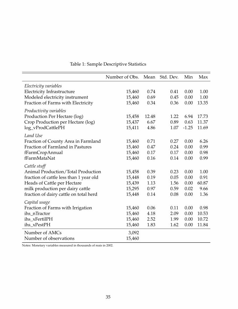
Table 1: Sample Descriptive Statistics

Number of Obs. Mean Std. Dev. Min Max

Electricity variablesElectricity Infrastructure 15,460 0.74 0.41 0.00 1.00Modeled electricity instrument 15,460 0.69 0.45 0.00 1.00Fraction of Farms with Electricity 15,460 0.34 0.36 0.00 13.35

Productivity variablesProduction Per Hectare (log) 15,458 12.48 1.22 6.94 17.73Crop Production per Hectare (log) 15,437 6.67 0.89 0.63 11.37log_vProdCattlePH 15,411 4.86 1.07 -1.25 11.69

Land UseFraction of County Area in Farmland 15,460 0.71 0.27 0.00 6.26Fraction of Farmland in Pastures 15,460 0.47 0.24 0.00 0.99fFarmCropAnnual 15,460 0.17 0.17 0.00 0.98fFarmMataNat 15,460 0.16 0.14 0.00 0.99

Cattle stuffAnimal Production/Total Production 15,458 0.39 0.23 0.00 1.00fraction of cattle less than 1 year old 15,448 0.19 0.05 0.00 0.91Heads of Cattle per Hectare 15,439 1.13 1.56 0.00 60.87milk production per dairy cattle 15,295 0.97 0.59 0.02 9.66fraction of dairy cattle on total herd 15,448 0.14 0.08 0.00 1.36

Capital usageFraction of Farms with Irrigation 15,460 0.06 0.11 0.00 0.98ihs_nTractor 15,460 4.18 2.09 0.00 10.53ihs_xFertilPH 15,460 2.52 1.99 0.00 10.72ihs_xPestPH 15,460 1.83 1.62 0.00 11.84

Number of AMCs 3,092Number of observations 15,460

Notes: Monetary variables measured in thousands of reais in 2002.

35

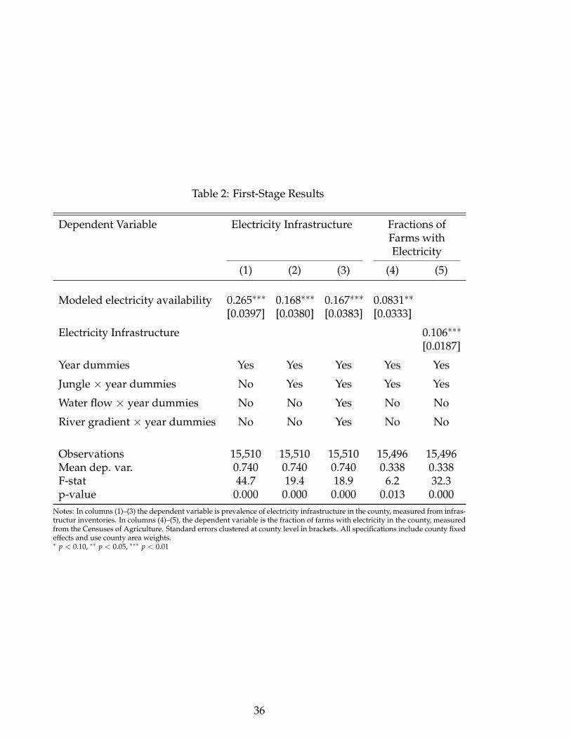
Table 2: First-Stage Results

Dependent Variable Electricity Infrastructure Fractions ofFarms withElectricity

(1) (2) (3) (4) (5)

Modeled electricity availability 0.265∗∗∗ 0.168∗∗∗ 0.167∗∗∗ 0.0831∗∗

[0.0397] [0.0380] [0.0383] [0.0333]

Electricity Infrastructure 0.106∗∗∗

[0.0187]

Year dummies Yes Yes Yes Yes Yes

Jungle × year dummies No Yes Yes Yes Yes

Water flow × year dummies No No Yes No No

River gradient × year dummies No No Yes No No

Observations 15,510 15,510 15,510 15,496 15,496Mean dep. var. 0.740 0.740 0.740 0.338 0.338F-stat 44.7 19.4 18.9 6.2 32.3p-value 0.000 0.000 0.000 0.013 0.000

Notes: In columns (1)–(3) the dependent variable is prevalence of electricity infrastructure in the county, measured from infras-tructur inventories. In columns (4)–(5), the dependent variable is the fraction of farms with electricity in the county, measuredfrom the Censuses of Agriculture. Standard errors clustered at county level in brackets. All specifications include county fixedeffects and use county area weights.∗ p < 0.10, ∗∗ p < 0.05, ∗∗∗ p < 0.01

36

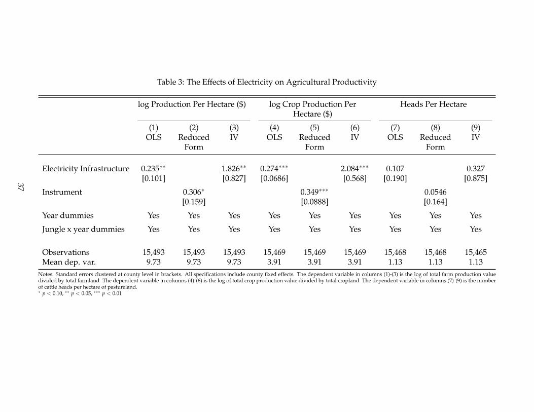
Table 3: The Effects of Electricity on Agricultural Productivity

log Production Per Hectare ($) log Crop Production PerHectare ($)

Heads Per Hectare

(1) (2) (3) (4) (5) (6) (7) (8) (9)OLS Reduced

FormIV OLS Reduced

FormIV OLS Reduced

FormIV

Electricity Infrastructure 0.235∗∗ 1.826∗∗ 0.274∗∗∗ 2.084∗∗∗ 0.107 0.327[0.101] [0.827] [0.0686] [0.568] [0.190] [0.875]

Instrument 0.306∗ 0.349∗∗∗ 0.0546[0.159] [0.0888] [0.164]

Year dummies Yes Yes Yes Yes Yes Yes Yes Yes Yes

Jungle x year dummies Yes Yes Yes Yes Yes Yes Yes Yes Yes

Observations 15,493 15,493 15,493 15,469 15,469 15,469 15,468 15,468 15,465Mean dep. var. 9.73 9.73 9.73 3.91 3.91 3.91 1.13 1.13 1.13

Notes: Standard errors clustered at county level in brackets. All specifications include county fixed effects. The dependent variable in columns (1)-(3) is the log of total farm production valuedivided by total farmland. The dependent variable in columns (4)-(6) is the log of total crop production value divided by total cropland. The dependent variable in columns (7)-(9) is the numberof cattle heads per hectare of pastureland.∗ p < 0.10, ∗∗ p < 0.05, ∗∗∗ p < 0.01

37

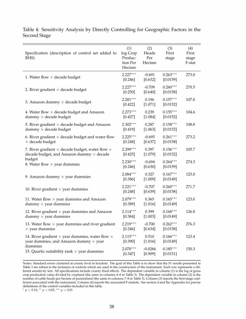
Table 4: Sensitivity Analysis by Directly Controlling for Geographic Factors in theSecond Stage

(1) (2) (3) (4)Specification (description of control set added toRHS)

log CropProduc-tion PerHectare

HeadsPer

Hectare

Firststage

FirststageF-stat

1. Water flow × decade budget 2.227∗∗∗ -0.691 0.263∗∗∗ 273.0[0.246] [0.632] [0.0159]

2. River gradient × decade budget 2.227∗∗∗ -0.709 0.260∗∗∗ 270.5[0.250] [0.640] [0.0158]

3. Amazon dummy × decade budget 2.281∗∗∗ 0.196 0.157∗∗∗ 107.0[0.422] [1.071] [0.0152]

4. Water flow × decade budget and Amazondummy × decade budget

2.273∗∗∗ 0.239 0.155∗∗∗ 104.6[0.427] [1.084] [0.0152]

5. River gradient × decade budget and Amazondummy × decade budget

2.302∗∗∗ 0.287 0.158∗∗∗ 108.8[0.419] [1.063] [0.0152]

6. River gradient × decade budget and water flow× decade budget

2.225∗∗∗ -0.695 0.261∗∗∗ 273.2[0.248] [0.637] [0.0158]

7. River gradient × decade budget, water flow ×decade budget, and Amazon dummy × decadebudget

2.299∗∗∗ 0.397 0.156∗∗∗ 105.7[0.425] [1.079] [0.0152]

8. Water flow × year dummies 2.230∗∗∗ -0.694 0.264∗∗∗ 274.3[0.246] [0.630] [0.0159]

9. Amazon dummy × year dummies 2.084∗∗∗ 0.327 0.167∗∗∗ 125.0[0.386] [1.009] [0.0149]

10. River gradient × year dummies 2.221∗∗∗ -0.707 0.260∗∗∗ 271.7[0.248] [0.639] [0.0158]

11. Water flow × year dummies and Amazondummy × year dummies

2.079∗∗∗ 0.365 0.165∗∗∗ 123.0[0.389] [1.016] [0.0149]

12. River gradient × year dummies and Amazondummy × year dummies

2.114∗∗∗ 0.399 0.168∗∗∗ 126.8[0.384] [1.003] [0.0149]

13. Water flow × year dummies and river gradient× year dummies

2.219∗∗∗ -0.700 0.262∗∗∗ 276.3[0.246] [0.634] [0.0158]

14. River gradient × year dummies, water flow ×year dummies, and Amazon dummy × yeardummies

2.115∗∗∗ 0.510 0.166∗∗∗ 123.4[0.390] [1.016] [0.0149]

15. Quartic suitability rank × year dummies 2.070∗∗∗ -0.0284 0.185∗∗∗ 150.3[0.347] [0.909] [0.0151]

Notes: Standard errors clustered at county level in brackets. The goal of this Table is to show that the IV results presented inTable 3 are robust to the inclusion of controls which are used in the construction of the instrument. Each row represents a dif-ferent sensitivity test. All specifications include county fixed effects. The dependent variable in column (1) is the log of grosscrop production value divided by cropland (the same in columns 4–6 in Table 3). The dependent variable in column (2) is thenumber of cattle heads per hectare of pastureland (the same in columns 7–8 in Table 3). Column (3) reports the first-stage coef-ficient associated with the instrument. Column (4) reports the associated F-statistic. See section 4 and the Appendix for precisedefinitions of the control variables included in this table.∗ p < 0.10, ∗∗ p < 0.05, ∗∗∗ p < 0.01

38

Table 5: The Effects of Electricity on the Allocation of Land

FarmlandCounty Area

PasturesFarmland

CroplandFarmland

Native VegetationFarmland

(1) (2) (3) (4) (5) (6) (7) (8)OLS IV OLS IV OLS IV OLS IV

Electricity Infrastructure 0.00987 0.288∗∗∗ 0.0223 −0.329∗∗∗ −0.0157 0.0369 0.0236 0.317∗∗∗

[0.0140] [0.110] [0.0191] [0.112] [0.0105] [0.0466] [0.0201] [0.109]

Year dummies Yes Yes Yes Yes Yes Yes Yes Yes

Jungle x year dummies Yes Yes Yes Yes Yes Yes Yes Yes

Observations 15,460 15,460 15,460 15,460 15,460 15,460 15,460 15,460Mean dep. var. 0.71 0.71 0.47 0.47 0.17 0.17 0.16 0.16

Notes: Standard errors clustered at county level in brackets. All specifications include county fixed effects. The dependent variable in columns (1)-(2) is the county’s farm area divided by thecounty’s total area. The dependent variable in columns (3)-(4) is the county’s area in pastures divided by the county’s farm area. The dependent variable in columns (5)-(6) is the county’s area incrops divided by the county’s farm area. The dependent variable in columns (7)-(8) is the county’s area in pastures divided by the county’s farm area∗ p < 0.10, ∗∗ p < 0.05, ∗∗∗ p < 0.01

39

Table 6: The Effects of Electricity on the Allocation of Land: Long Run

FarmlandCounty Area

PasturesFarmland

CroplandFarmland

Native VegetationFarmland

(1) (2) (3) (4) (5) (6) (7) (8)OLS IV OLS IV OLS IV OLS IV

Electricity Infrastructure −0.0189 0.0948 −0.00580 −0.430∗∗∗ −0.0110 0.0744 0.0543∗∗∗ 0.331∗∗∗

[0.0136] [0.107] [0.0195] [0.117] [0.0116] [0.0474] [0.0206] [0.126]

Year dummies Yes Yes Yes Yes Yes Yes Yes Yes

Jungle x year dummies Yes Yes Yes Yes Yes Yes Yes Yes

Observations 12,368 12,368 12,368 12,368 12,368 12,368 12,368 12,368Mean dep. var. 0.71 0.71 0.47 0.47 0.17 0.17 0.16 0.16

Notes: Standard errors clustered at county level in brackets. All specifications include county fixed effects. This table is similar to Table 6, except that the dependent variables are forward-laggedby one decade. The dependent variable in columns (1)-(2) is the county’s farm area divided by the county’s total area. The dependent variable in columns (3)-(4) is the county’s area in pasturesdivided by the county’s farm area. The dependent variable in columns (5)-(6) is the county’s area in crops divided by the county’s farm area. The dependent variable in columns (7)-(8) is thecounty’s area in pastures divided by the county’s farm area∗ p < 0.10, ∗∗ p < 0.05, ∗∗∗ p < 0.01

40

Table 7: The Effects of Electricity on Crop Choices

log Production (tons) log Area (ha) Area/Farmland

(1) (2) (3) (4) (5) (6)OLS IV OLS IV OLS IV

Panel A: Grains

Electricity Infrastructure 0.206 3.752∗∗∗ 0.042 2.155∗∗ 0.012∗ 0.200∗∗∗

[0.230] [1.227] [0.215] [1.071] [0.007] [0.046]Observations 15,460 15,460 15,460 15,460 15,460 15,460Mean dep. var. 7.57 7.57 7.54 7.54 0.13 0.13

Panel B: Cassava

Electricity Infrastructure 0.332∗∗∗ 0.494 0.082 −0.426 −0.004 −0.032∗∗

[0.112] [0.863] [0.105] [0.827] [0.004] [0.016]Observations 15,423 15,423 15,423 15,423 15,423 15,423Mean dep. var. 4.87 4.87 3.18 3.18 0.01 0.01

Notes: The table shows that electrification has effects on the crop mix. Some crops benefit more from electrification than others. Grains, in particular, benefit from electrification through irriga-tion, handling and storage, and mecanization in general. Cassava, on the other hand, benefits less from electrification, as it is a typical subsistence crop. Consistent with this, the table shows thatan increase in electricity infrastructure leads to a shit into grains and out of cassava – production and area increase (respectively, decrease) for grains (respectively, cassava). The table makes thepoint that the shift from land-intensive towards capital-intensive activities happens also between crops, and not only between cattle grazing and crops. This fact helps explaining why we seelittle effect of electricity on the share of farmland allocated to crops in Table 5. Farmers may be switching crops, keeping overall cropland as a fraction of farmland roughly constant.∗ p < 0.10, ∗∗ p < 0.05, ∗∗∗ p < 0.01

41

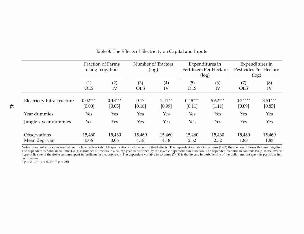
Table 8: The Effects of Electricity on Capital and Inputs

Fraction of Farmsusing Irrigation

Number of Tractors(log)

Expenditures inFertilizers Per Hectare

(log)

Expenditures inPesticides Per Hectare

(log)

(1) (2) (3) (4) (5) (6) (7) (8)OLS IV OLS IV OLS IV OLS IV

Electricity Infrastructure 0.02∗∗∗ 0.13∗∗∗ 0.17 2.41∗∗ 0.48∗∗∗ 5.62∗∗∗ 0.24∗∗∗ 3.51∗∗∗

[0.00] [0.05] [0.18] [0.99] [0.11] [1.11] [0.09] [0.85]

Year dummies Yes Yes Yes Yes Yes Yes Yes Yes

Jungle x year dummies Yes Yes Yes Yes Yes Yes Yes Yes

Observations 15,460 15,460 15,460 15,460 15,460 15,460 15,460 15,460Mean dep. var. 0.06 0.06 4.18 4.18 2.52 2.52 1.83 1.83

Notes: Standard errors clustered at county level in brackets. All specifications include county fixed effects. The dependent variable in columns (1)-(2) the fraction of farms that use irrigation.The dependent variable in columns (3)-(4) is number of tractors in a county-year transformed by the inverse hyperbolic sine function. The dependent variable in columns (5)-(6) is the inversehyperbolic sine of the dollar amount spent in fertilizers in a county-year. The dependent variable in columns (7)-(8) is the inverse hyperbolic sine of the dollar amount spent in pesticides in acounty-year.∗ p < 0.10, ∗∗ p < 0.05, ∗∗∗ p < 0.01

42

Table 9: Cattle grazing productivity really doesn’t go up with electrification?

Animal Prod./Total Prod. Fraction Cattle ≤ 1 yo Heads Per Hectare Milk per Dairy Cattle (1000liters)

Fraction of Dairy Cattle

(1) (2) (3) (4) (5) (6) (7) (8) (9) (10)OLS IV OLS IV OLS IV OLS IV OLS IV

Electricity Infrastructure 0.0205 −0.333∗∗∗ 0.00337 0.0216 0.106 −0.0728 0.0497 0.561∗∗∗ 0.0100∗∗ 0.0650∗∗

[0.0210] [0.117] [0.00355] [0.0194] [0.190] [0.593] [0.0310] [0.171] [0.00402] [0.0260]

Observations 15,458 15,458 15,448 15,448 15,439 15,438 15,295 15,292 15,448 15,448Mean dep. var. 0.388 0.388 0.191 0.191 1.130 1.130 0.971 0.971 0.139 0.139

Notes: The table makes the following three points: (i) consistent with the story that electrification increases crop productivity relative to cattle grazing productivity, columns 1-2 show that thefraction of animal production on overall farm production decreases. (Note that includes poltry production which is likely affected by electricity); (ii) the result in Table 3 is robust to the measureof cattle grazing productivity we use. In this table, we use two alternative measures of cattle grazing productivity instead of Cattle Production Per Hectare of Pastureland. Columns 3-4 use thefraction of young herd on overall herd – the idea being that the younger the herd becomes ready for the slaughterhouse, the more productive the farm is (unfourtunately we don’t have the herd’sage). Columns 5-6 use the stocking ratio – heads of cattle per hectare of pastureland. The IV estimates are not significant, not have meaninful magnitudes when either measure is used. (iii) Dairycattle productivity does go up – columns 7-8 show that a 10% increase in electrification increases milk per cow by 60 liters, a 6% increase on the mean. However, this effect is small for it does notinduce producers to change the herd’s composition towards dairy cattle, as shown in columns 9-10.∗ p < 0.10, ∗∗ p < 0.05, ∗∗∗ p < 0.01

43

Table 10: The Effects of Electricity on Forestry Production

log ForestryProduction Value

log Production Valueof Wood Products

log ForestryProduction Value Per

Hectare of Forest

Share of PlantedForests on Farmland

(1) (2) (3) (4) (5) (6) (7) (8)OLS IV OLS IV OLS IV OLS IV

Electricity Infrastructure -0.371∗∗ 0.129 -0.300 -0.177 -0.383∗∗∗ -2.508 -0.00174 -0.0133[0.150] [1.874] [0.202] [1.982] [0.140] [1.728] [0.00221] [0.0244]

Observations 15,510 15,510 15,510 15,510 15,462 15,462 15,496 15,496Mean dep. var. 8.664 8.664 4.309 4.309 0.165 0.165 0.0172 0.0172

Notes: Standard errors clustered at county level in brackets. All specifications use county area weights and include county fixed effects, year fixed effects, and Amazon-year dummy interactions.∗ p < 0.10, ∗∗ p < 0.05, ∗∗∗ p < 0.01

44

Table 11: Teting for the presence of credit constraints: Do past rainfall schocks affectproductivity and investments?

Number of Tractors log Production Per Hectare ($)

(1) (2) (3) (4) (5) (6)

Rainfall at t 28.97∗ 23.31 49.27∗∗ 0.0225 0.00647 0.0252[17.37] [17.25] [19.52] [0.0240] [0.0239] [0.0242]

Rainfall at t-1 24.85∗∗∗ 0.108∗∗∗

[4.813] [0.0156]

Rainfall at t-3 57.67∗∗∗ 0.0717∗∗∗

[16.38] [0.0268]

Rainfall at t-5 113.7∗∗∗ 0.0745∗∗∗

[19.01] [0.0185]

Observations 15,510 15,510 15,510 15,493 15,493 15,493Mean dep. var. 169.9 169.9 169.9 9.725 9.725 9.725

Notes: Standard errors clustered at county level in brackets. All specifications use county area weights and include countyfixed effects, year fixed effects, and Amazon-year dummy interactions.∗ p < 0.10, ∗∗ p < 0.05, ∗∗∗ p < 0.01

45

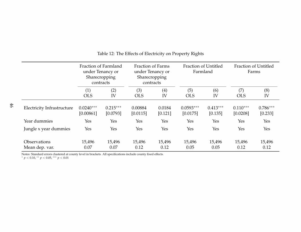
Table 12: The Effects of Electricity on Property Rights

Fraction of Farmlandunder Tenancy or

Sharecroppingcontracts

Fraction of Farmsunder Tenancy or

Sharecroppingcontracts

Fraction of UntitledFarmland

Fraction of UntitledFarms

(1) (2) (3) (4) (5) (6) (7) (8)OLS IV OLS IV OLS IV OLS IV

Electricity Infrastructure 0.0240∗∗∗ 0.215∗∗∗ 0.00884 0.0184 0.0593∗∗∗ 0.413∗∗∗ 0.110∗∗∗ 0.786∗∗∗

[0.00861] [0.0793] [0.0115] [0.121] [0.0175] [0.135] [0.0208] [0.233]

Year dummies Yes Yes Yes Yes Yes Yes Yes Yes

Jungle x year dummies Yes Yes Yes Yes Yes Yes Yes Yes

Observations 15,496 15,496 15,496 15,496 15,496 15,496 15,496 15,496Mean dep. var. 0.07 0.07 0.12 0.12 0.05 0.05 0.12 0.12

Notes: Standard errors clustered at county level in brackets. All specifications include county fixed effects.∗ p < 0.10, ∗∗ p < 0.05, ∗∗∗ p < 0.01

46

9 Appendix

9.1 Calculating the effect of electricity on native vegetation

Column (10) of Table 5 gives us the effect of electricity on native vegetation insidefarms. Because we do not have explicit data on native vegetation outside farms, weneed one assumption to be able to back out the effect of electricity on overall nativevegetation. To see this, first note that V(e) = VI(e) + VO(e), where V is total na-tive vegetation, VI denotes native vegetation inside of farms, and VO denotes nativevegetation outside of farms. Denoting county area by C, we are interested in

∂

∂eV(e)

C=

∂

∂eVI(e)

C+

∂

∂eVO(e)

C(13)

From the numbers in Table 5 we can back out the term ∂∂e

VI(e)C using the chain rule.

But since we do not have data on VOC , we must make one assumption to fully recover

the effect of electricity on overall native vegetation. Note that we can write VO(e) =k(C − F(e)), that is, native vegetation outside of farms is a fraction k of the countyarea (C) that is not in farms (F(e)). Plugging that on the second term on the RHS of(13),

∂

∂eVO(e)

C=

∂

∂ek(C− F(e))

C= −k

∂

∂eF(e)

C(14)

We have ∂∂e

F(e)C from column (2) of Table 5. The only information we do not have

is k, the fraction of the county area outside of farms that is in native vegetation.Assuming k = 1 (k = 0) gives us a lower (upper) bound on the effect of electricityon overall native vegetation.

To calculate ∂∂e

VI(e)C , note that the IV coefficient in column (10) of Table 5 gives us

∂∂e

VI(e)F(e) which, by applying the chain rule, is

∂VI∂e ·F(e)−VI(e)· ∂F

∂eF(e)2 . Solving for ∂VI

∂e anddividing both sides by C yields

∂

∂eVI

C=

∂

∂eVI(e)F(e)

· F(e)C

+VI

F(e)· ∂

∂eF(e)

C(15)

Plugging equations (14) and (15) into (13),

∂

∂eV(e)

C=

∂

∂eVI(e)F(e)

· F(e)C

+ (VI

F(e)− k) · ∂

∂eF(e)

C(16)

If we evaluate this derivative at the sample means, Table 5 gives all the terms on theRHS of this equation except for k. The effect of electricity on the share of farmland in

47

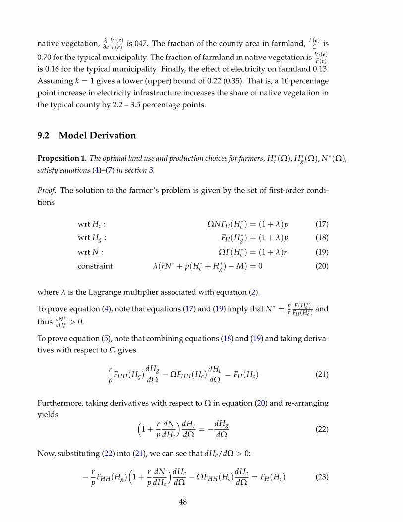
native vegetation, ∂∂e

VI(e)F(e) is 047. The fraction of the county area in farmland, F(e)

C is

0.70 for the typical municipality. The fraction of farmland in native vegetation is VI(e)F(e)

is 0.16 for the typical municipality. Finally, the effect of electricity on farmland 0.13.Assuming k = 1 gives a lower (upper) bound of 0.22 (0.35). That is, a 10 percentagepoint increase in electricity infrastructure increases the share of native vegetation inthe typical county by 2.2 – 3.5 percentage points.

9.2 Model Derivation

Proposition 1. The optimal land use and production choices for farmers, H∗c (Ω), H∗g(Ω), N∗(Ω),satisfy equations (4)–(7) in section 3.

Proof. The solution to the farmer’s problem is given by the set of first-order condi-tions

wrt Hc : ΩNFH(H∗c ) = (1 + λ)p (17)

wrt Hg : FH(H∗g) = (1 + λ)p (18)

wrt N : ΩF(H∗c ) = (1 + λ)r (19)

constraint λ(rN∗ + p(H∗c + H∗g)−M) = 0 (20)

where λ is the Lagrange multiplier associated with equation (2).

To prove equation (4), note that equations (17) and (19) imply that N∗ = pr

F(H∗c )FH(H∗c )

and

thus ∂N∗∂H∗c

> 0.

To prove equation (5), note that combining equations (18) and (19) and taking deriva-tives with respect to Ω gives

rp

FHH(Hg)dHg

dΩ−ΩFHH(Hc)

dHc

dΩ= FH(Hc) (21)

Furthermore, taking derivatives with respect to Ω in equation (20) and re-arrangingyields (

1 +rp

dNdHc

)dHc

dΩ= −

dHg

dΩ(22)

Now, substituting (22) into (21), we can see that dHc/dΩ > 0:

− rp

FHH(Hg)(

1 +rp

dNdHc

)dHc

dΩ−ΩFHH(Hc)

dHc

dΩ= FH(Hc) (23)

48

Electrification therefore increases the productivity of N and induces farmers to in-vest in more N. N is useful for cultivation, which increases the land allocated tocultivation. This necessarily leads credit constrained farmers to lower land allocatedto cattle grazing, because a larger share of their budget is spent on cultivation.

The net effect on native vegetation within the farm will depend on farmers’ total landdemand across cultivation and grazing. We define the farmer’s total land demandas H f = Hc + Hg, equation 22 can be rearranged to:

dH f

dΩ=

dHc

dΩ+

dHg

dΩ= − r

pdNdHc

dHc

dΩ< 0 (24)

The total land demand for all forms of agricultural activities decreases, because farm-ers have to spend more money on N. In summary, the model predicts that electrifica-tion (i.e. increasing the productivity of the limited factor) will: (i) increase use of N,(ii) induce farmers to shift land use from land-intensive cattle grazing to N-intensivecultivation; and (iii) reduce farmers’ total land demand.

The net effect of electrification on deforestation will depend not only on intensive-margin changes in land demand within each farm, but also on how the productivityshock induces extensive-margin changes in the decision to enter the agricultural sec-tor. To analyze this net effect, we define the total area of native vegetation as

Hv = H −∫

θ<ΠH f dΓ(θ)

= H − H f Γ(Π). (25)

The total derivative of the forest with respect to electrification displays two opposingeffects:

dHv

dΩ= −dΓ(Π)

dΠdΠdΩ

H f −Γ(Π)dH f

dΩ

= −γ(Π)KF(Ha)H f −Γ(Π)dH f

dΩ(26)

< 0 > 0

Proposition 2. The effect of electrification on overall native vegetation defined in equation(8) is ambiguous.

49

Proof. The total derivative of the forest with respect to electrification displays twoopposing effects:

dHv

dΩ= −

dHc + dHg

dΩΓ(θ)− (Hc + Hg)Γ(θ)[

dΠdΩ− dθ

dΩ] (27)

dHv

dΩ= −dΓ(Π)

dΠdΠdΩ

H f −Γ(Π)dH f

dΩ

= −γ(Π)KF(Ha)H f −Γ(Π)dH f

dΩ(28)

< 0 > 0

References

Acemoglu, D. and Johnson, S. (2005). Unbundling institutions. Journal of PoliticalEconomy, 113(5):949–995.

BenYishay, A. and Mobarak, A. M. (2014). Social Learning and Communication.NBER Working Papers 20139, National Bureau of Economic Research, Inc.

BRASIL (2007). Balanco energetico nacional 2007: ano base 2006. Technical Re-port 194 p, Ministerio de Minas e Energia, EPE, Rio de Janeiro. available athttps://ben.epe.gov.br/downloads/BEN2007_Versao_Completa.pdf.

Conley, T. G. and Udry, C. R. (2010). Learning about a new technology: pineapple inGhana. American Economic Review, 100(1):35–69.

Conning, J. and Udry, C. (2007). Rural Financial Markets in Developing Countries, vol-ume 3 of Handbook of Agricultural Economics, chapter 56, pages 2857–2908. Elsevier.

Cropper, M. and Griffiths, C. (1994). The Interaction of Population Growth and En-vironmental Quality. American Economic Review, 84(2):250–54.

Cropper, M., Griffiths, C., and Jyotsna (2001). Predicting Spatial Patterns of Defor-estation: The Role of Roads and Protected Areas in North Thailand. Land Eco-nomics, May.

50

Cropper, M., Griffiths, C., and Mani, M. (1999). Roads, Population Pressures, andDeforestation in Thailand, 1976-1989. Land Economics, 75 (1):58–73.

Dinkelman, T. (2011). The Effects of Rural Electrification on Employment: New Evi-dence from South Africa. American Economic Review, 101(7):3078–3108.

Donaldson, D. (forthcoming). Railroads of the raj: Estimating the impact of trans-portation infrastructure. American Economic Review.

Duflo, E. and Pande, R. (2007). Dams. The Quarterly Journal of Economics, 122(2):pp.601–646.

Foster, A. D. and Rosenzweig, M. R. (2003). Economic growth and the rise of forests.The Quarterly Journal of Economics, 118(2):pp. 601–637.

Grossman, G. M. and Krueger, A. B. (1991). Environmental impacts of a north amer-ican free trade agreement. National Bureau of Economic Research Working Paper 3914,NBER, Cambridge MA.

Grossman, G. M. and Krueger, A. B. (1995). Economic growth and the environment.Quarterly Journal of Economics, 110:353–377.

Hidalgo, F. D., Naidu, S., Nichter, S., and Richardson, N. (2010). Economic determi-nants of land invasions. The Review of Economics and Statistics, 92(3):505–523.

Hornbeck, R. (2010). Barbed wire: Property rights and agricultural development.The Quarterly Journal of Economics, 125(2):767–810.

Hornbeck, R. and Keskin, P. (2014). The historically evolving impact of the ogallalaaquifer: Agricultural adaptation to groundwater and drought. American EconomicJournal: Applied Economics, 6(1):190–219.

Lipscomb, M., Mobarak, A. M., and Barham, T. (2013). Development Effects of Elec-trification: Evidence from the Topographic Placement of Hydropower Plants inBrazil. American Economic Journal: Applied Economics, 5(2):200–231.

Matsuura, K. and Willmott, C. (2012). Terrestrial precipitation: 1900-2010 griddedmonthly time series (1900 - 2010) (v 3.01 added 6/14/12). Technical report, Uni-versity of Delaware. University of Delaware. http://climate.geog.udel.edu/ cli-mate/.

MMA (2013). Sistema Nacional de Unidadades de Conservação, SNUC. Database,Ministério do Meio Ambiente.

Pfaff, A. (1999). What Drives Deforestation in the Brazilian Amazon? Evidence from

51

Satellite and Socioeconomic Data. Journal of Environmental Economics and Manage-ment, 37(1):26–43.

Rud, J. P. (2012). Electricity provision and industrial development: Evidence fromindia. Journal of Development Economics, 97:352–367.

Sekhri, S. (2011). Public provision and protection of natural resources: Groundwaterirrigation in rural india. Amercian Economic Journal: Applied Economics, 3(4):29–55.

Stavins, R. N. and Jaffe, A. B. (1990). Unintended Impacts of Public Investments onPrivate Decisions: The Depletion of Forested Wetlands. The American EconomicReview, 80(3):pp. 337–352.

Stern, N. (2008). The economics of climate change. American Economic Review,98(2):1–37.

World Bank (1990). Brazil - irrigation subsector review. Sector Report 7797, WorldBank.

Zomer, R. J., Trabucco, A., Coe, R., and Place, F. (2014). Trees on farms: an updateand reanalysis of agroforestry’s global extent and socio-ecological characteristics.World Agroforestry Center Working Paper 179.

52