agroscope reckenholz-tänikon research station art · pdf fileagroscope...

Federal Department of Economic Affairs FDEA

Agroscope Reckenholz-Tänikon Research Station ART

October 2013

Life Cycle Assessment of Agricultural Systems:

Introduction

Thomas Nemecek

Agroscope Reckenholz-Tänikon Research Station ART CH-8046 Zurich, Switzerland

http://www.agroscope.ch [email protected]

http://www.agroscope.ch/

mailto:[email protected]

2

Oveview

Specific aspects of agriculture

Consequences for agricultural LCA

Defining system boundaries

Defining the functional unit

Impact assessment for biodiversity and soil quality

Variability of agricultural production and use of multivariate

statistics

Examples of application of LCA:

Cropping system analysis

Animal production, meat, milk and cheese

Biofuels

Environmental assessment of farms

Introduction to agricultural LCA

Thomas Nemecek | © Agroscope Reckenholz-Tänikon Research Station ART

3

Specific aspects of agricultural systems

Strong reliance on natural resources: land, water, sunlight,

nutrients, soil, biodiversity

Dependence on living organisms

Open systems

Processes are difficult to control: e.g. nutrient leaching,

erosion, N2O emissions

Emissions are difficult to measure, due to the open nature of

the systems

Small-scale structure: numerous farm businesses

Complex systems, only partly understood

Nonlinear nature of many environmental mechanisms

High variability of processes and products, due to soil,

climate, topography, agricultural management, traditions



4

Consequences of these specificities of agriculture (1) Environmental models and data need to be developed or

adapted to agriculture

Account for non-linear relationships of environmental

processes

Difficulty to clearly delimit the ecosphere (environmental

system) and the technosphere (economic system): e.g.

agricultural soil, biodiversity in the field

Due to the variability a large number of observations is

needed to get representative data (but often insufficient

resources)

Efficient LCA databases and calculation procedures are

required to manage this large number of observations



5

Consequences of these specificities of agriculture (2)

Since measurements at a large scale are not feasible

environmental models are needed, reflecting the main

influencing factors

Need to include specific impact categories, related to the use

of natural resources: land use, land use change, biodiversity,

soil quality, water resources

Need to adapt some impact categories, e.g. impact of

pesticides on ecotoxicity

Collaboration between agronomists, environmental scientists

and local experts is required



6

Fossil energy and carbon footprint are not enough for agricultural systems



x = agricultural products

Fossil energy use is identified by all

methodologies as the most important

driver of environmental burden of the

majority of the commodities included, with

the main exception of agricultural

Products (x). Huijbreghts et al. (2010)

7

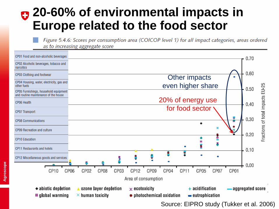
20-60% of environmental impacts in Europe related to the food sector



Source: EIPRO study (Tukker et al. 2006)

20% of energy use

for food sector

Other impacts

even higher share

8



Defining system boundaries: Temporal system boundaries

Annual crops:

Starting after harvest of previous crop (including fallow period

or catch crop, if no product)

Ending with harvest of the considered crop

Permanent crops:

Annual basis (1st January to 31st December) or

Multiannual cropping cycle (distinguishing different phases:

planting, young plantation, main yielding phase, eradication)

9



Single crop or cropping system?

YearMonth 1 2 3 4 5 6 7 8 9 10 11 12 1 2 3 4 5 6 7 8 9 10 11 12 1 2 3 4 5 6 7 8 9 10 11 12

Year 4 5 6Month 1 2 3 4 5 6 7 8 9 10 11 12 1 2 3 4 5 6 7 8 9 10 11 12 1 2 3 4 5 6 7 8 9 10 11 12

Spring

barleyGrass-clover mixture ...

Fa

llo

w ...

... F

allo

w

1 2 3

... G

ras

s-

clo

ve

r m

ixtu

re

PotatoesG

ree

n m

an

ure

Winter wheat Forage catch crop Grain maize

10



Methodology: Crop combinations

1 2 3 Year Month 1 2 3 4 5 6 7 8 9 10 11 12 1 2 3 4 5 6 7 8 9 10 11 12 1 2 3 4 5 6 7 8 9 10 11 12

Fa

llo

w ...

Oil Seed

Rape Winter Wheat Winter Barley

Fa

llo

w ...

Fa

llo

w ...

Oil

Se

ed

Ra

pe

Crop Rotation

Crop Combination F

all

ow

...

Oil Seed

Rape Winter Wheat

Fall

ow

...

Winter wheat Winter Barley

Fa

llo

w ...

Winter Barley

Fall

ow

...

Oil Seed

Rape 1

2

3

11

Comparison of different crop rotations with (P) and without (S) pea



0

0.05

0.1

0.15

0.2

0.25

0.3

0.35

0.4

0

20

40

60

80

100

120

S1 S2 P1 P2 P3 S1 S2 P1 P2 P3 S1 S2 P1 P2 P3 S1 S2 P1 P2 P3

Beauce_Con Beauce_INT Burgundy Moselle

kg N-eq

/€

kg N

-eq

/ha/

a

mechanisation N fertiliser P/K fertiliser field emissions

irrigation seed pesticides per € gross margin II

Source: Hayer et al. (2011)

12

Relationship between N fertilisation and global warming potential



R² = 0.97

R² = 0.92

R² = 0.96

R² = 0.95

2000

2400

2800

3200

3600

75 100 125 150 175

kg C

O2-

eq/h

a/a

N-fertiliser [kg N/ha]Beauce-M Beauce+M Burgundy Moselle

Source: Hayer et al. (2011)

13



Defining system boundaries: Example of crop production

Products:

Infrastructure:

•Buildings

•Machinery

Field work processes:

•Soil cultivation

•Fertilisation

•Sowing

•Chemical plant protection

•Mechanical treatment

•Harvest

•Transport

Field production

Catch crops

Silage maize

Sugar beets

Fodder beets

Beetroot

Carrots

Cabbage

Wheat

Barley

Rye

Oats

Grain maize

CCM

Faba beans

Soya beans

Protein peas

Sunflowers

Rape seed

Potatoes

Co-Product: Straw

Product treatment:

Grain drying

Potato grading

System boundary

Reso

urc

es

Direct and indirect emissions

Manure storage

Animal excrements

Animal production system

Inputs:

•Seed

•Fertilisers (min. & org.)

•Pesticides

•Energy carriers

•Irrigation water

14

Defining system boundaries: Farm/Animal products

Infrastructure

•Buildings

•Equipment

•Machines

Purchased inputs

•Energy carriers

•Fertilisers

•Seed

•Pesticides

•Feedstuffs, straw

•Animal

•Water

Field operations

•Tillage

•Sowing

•Fertilisation

•Maintenance

•Irrigation

•Harvest

•Transport to farm

Animal production

•Feeding

•Milking

•Manure management

•Grazing

Manure

storage Fodder

conservation Re

so

urc

es

Indirect emissions Direct emissions

System boundary = farm gate

Animal products

•Milk

•Meat

•Eggs

•Wool

Vegetal products,

e.g.

•Wheat

•Maize

•Potatoes

•Vegetables



15



Defining system boundaries: Where to draw the line between animal and plant production?

Animal production (incl. feedstuffs,

buildings, emissions, etc.)

Manure storage

and treatment

Manure application

(incl. machinery use and emissions)

Nutrient use in plant production

?

16



Multifunctionality of agriculture: Functions and functional units

1. Land management function: ha*year

goal: minimize land use intensity

2. Productive function: physical unit (MJ

gross calorific value) goal: optimise eco-

efficiency (minimal impact per produced

energy unit)

3. Financial function: monetary unit

goal: optimise eco-efficiency

(minimal impact per € gross margin 1)

17



SALCA methodology Method for biodiversity - framework

• 11 Indicator species groups were determined considering ecological

and LCA criteria: flora, birds, mammals, amphibians, molluscs, spiders,

carabids, butterflies, wild bees, and grasshoppers.

• Two characteristics: overall species diversity of the indicator species

groups and ecologically demanding species

• Extensive inventory data about agricultural practices: occupation,

emissions, farming intensity indicators (e.g. number of cuts) and

process figures (e.g. herbicide type). Beside typical cultivated fields,

semi-natural habitats were integrated.

• Characterisation based on scoring system was evolved to estimate

every indicator species group’s reaction to agricultural activities

followed by an aggregation step resulting in scores.

• Aggregation and normalisation of scores: biodiversity value and

biodiversity potential

18

LCA Food 2012 Saint Malo | 3 October 2012


AA-3

ISG-1

ISG-3

ISG-4

ISG-2

ISG-5

Biodiversity =

Indicator Species

Groups (ISG)

Birds

Butterflies

AA-1

AA-2

AA-4

AA-5

Agricultural

Activities (AA)

Mowing

Wild flower strips

Insecticide application

Estimation of impacts on biodiversity

Impact

Bottom-up approach: Scores based on scientific and expert knowledge

01/11/2013

Spiders

SALCA-Biodiversity

19

LCA Food 2012 Saint Malo | 3 October 2012


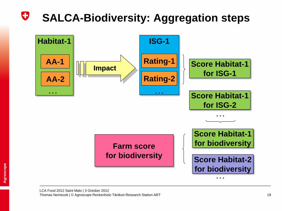
SALCA-Biodiversity: Aggregation steps

Impact

ISG-1

Rating-1

Rating-2

Habitat-1

Score Habitat-1

for biodiversity

AA-1

AA-2

…

Score Habitat-2

for biodiversity

… …

…

Farm score

for biodiversity

Score Habitat-1

for ISG-1

Score Habitat-1

for ISG-2

20



SALCA methodology Method for biodiversity – DOK trial

Biodiversity points D0 D1 D2 O1 O2 C1 C2 M2

Total aggregated 8.7 8.1 8.0 8.0 8.0 7.7 7.6 7.6

Flora arable land 14.8 13.9 13.9 13.8 13.8 12.8 12.6 12.5

Flora grassland 4.9 4.3 4.1 4.2 4.2 4.1 3.9 3.9

Birds 10.3 8.7 8.6 8.5 8.5 8.0 8.0 7.9

Small mammals 3.5 3.5 3.5 3.5 3.5 3.5 3.5 3.5

Amphibians 2.5 2.1 2.1 2.1 2.1 2.0 2.0 2.0

Molluscs 2.5 2.3 2.3 2.3 2.3 2.3 2.3 2.3

Spiders 13.9 13.2 13.2 13.0 13.0 12.2 12.0 12.1

Carabids 14.7 14.0 14.0 14.0 14.0 13.7 13.5 13.6

Butterflies 9.8 8.8 8.6 8.8 8.6 8.5 8.4 8.5

Wild bees 4.9 4.8 4.8 4.8 4.8 4.8 4.8 4.9

Grasshoppers 11.0 9.8 9.5 9.9 9.6 9.4 9.3 9.3

Amphibians 1.7 1.4 1.3 1.3 1.3 1.3 1.2 1.3

Spiders 13.4 12.7 12.6 12.5 12.4 11.6 11.5 11.6

Carabids 14.7 14.0 14.0 14.0 14.0 13.7 13.6 13.7

Butterflies 9.8 8.8 8.5 8.8 8.5 8.4 8.4 8.5

Grasshoppers 10.9 9.6 9.3 9.6 9.4 9.2 9.1 9.2

Higher values mean higher species richness

favourable

very favourable

Total species richness

Species with high ecological requirements

compared to reference C2

D = Bio-dynamic

O = Organic

C = Conventional

(mixed min./org.

fertilisation)

M = Conventional

(mineral fertilisation)

2 = normal

fertilisation level

1 = 50% fertilisation

level

0 = no fertilisation

Source: Nemecek et al. (2005)

21



no relevance for the considered system

SALCA methodology Method for biodiversity – case study 1/2

Results of SALCA-Biodiversity. Biodiversity scores

are given per ha cultivated crop. A, B, C, D are

management systems with main characteristics :

Winter wheat systems:

(A) Conventional production; 5.8t DM/ha

(B) Integrated production – intensive; 5.5t DM/ha

(C) Integrated production – extensive; 4.5t DM/ha

(D) Organic production; 3.5t DM/ha

Grassland systems (hay production):

(A) 5 cuts/year, fertilised with slurry; 11t DM/ha

(B) 4 cuts/year, fertilised with slurry; 9t DM/ha

(C) 3 cuts/year, fertilised with solid manure; 5.6t DM/ha

(D) 1 cut/year, no fertilisation; 2.7t DM/ha

Scores of grassland (A) and winter wheat (B) systems are

set as reference scores. Color codes are given for rough

comparison:

similar to the reference (95%<score<104%)

much better than the reference (score >115%)

better than the reference (105%<score<114%)

Grassland Winter Wheat

(D) (A) (B) (C) (D) (A) (B) (C)

Overall species diversity 6.2 6.4 13.8 21.3 7.7 7.5 8.4 8.7

Grassland flora 3.7 3.9 11.4 18.5

Crop flora 15.2 15.1 16.0 17.3

Birds 6.4 6.7 13.8 22.0 5.3 5.0 6.2 6.4

Mammals 7.3 7.3 11.1 11.1 4.6 4.6 4.6 4.6

Amphibians 2.1 2.1 5.2 9.5 1.7 1.7 1.8 1.8

Molluscs 5.4 5.6 5.8 11.3 2.2 2.2 2.2 2.2

Spiders 9.1 9.3 15.8 22.4 8.2 8.0 10.5 10.7

Carabid Beetles 7.0 7.4 13.6 21.0 10.9 10.6 11.7 11.9

Butterflies 6.8 7.0 20.0 36.0

Wild Bees 7.4 7.6 18.6 23.0 5.2 4.9 5.0 4.8

Grasshoppers 6.9 6.9 19.4 33.1

Amphibians 0.8 0.8 2.9 4.8 1.5 1.4 1.6 1.6

Spiders 8.9 9.0 15.3 21.6 8.0 7.8 10.3 10.5

Carabid Beetles 7.0 7.3 13.4 20.6 10.6 10.1 11.2 11.3

Butterflies 6.7 6.8 19.4 36.0

Grasshoppers 6.8 6.8 19.3 32.9

Biodiversity scores

Production system

Species with high ecological requirements

Source: Jeanneret et al. 2006

23 Introduction to agricultural LCA


Physical Rooting depth of soil

Macropore volume

Aggregate stability

Chemical Soil organic matter

Inorganic pollutants

Organic pollutants

Biological Earthworm biomass

Microbial biomass

Microbial activity

SALCA methodology Method for soil quality - framework

Spatial system boundary = farm;

Temporal system boundary = crop rotation period (6-8 years)

Management data of all plots of a farm in a single year are

considered as representative for a whole crop rotation

Only influences of agricultural management practices are included,

not immissions

The development trend of soil properties is assessed, not absolute

values

Criteria

According to ISO 14040 and ISO

14042

Depending on the needs of Life

Cycle Assessment

Soil properties

Physical

Chemical

Biological

9 D

ire

ct

Ind

ica

tors

=

me

asu

rab

le s

oil

pro

pe

rtie

s

Source: Oberholzer et al. (2006)

24



Risk of soil com-

paction by wheeling

Number of applica-

tions per year with

possibly toxic effects

Amount of organic

substances

Humus balance

Impact classes

SALCA methodology Method for soil quality – impact assessment

Pro

cesses

Direct indicators

Soil organic matter

Microbial biomass

Microbial activity

Earthworm biomass

Macropore volume

Aggregate stability

Management data

Slurry

application

Soil texture

Soil moisture

Soil structure

Figure 1: Example of impact assessment of a slurry application

Example: slurry application



SALCA methodology Method for soil quality – example DOK

No fer-

tiliser D0

Bio-dyna-

mic D2

Bio-orga-

nic O2

Conventiona

l

K2

Mineral

fertiliser M

Soil tillage ploughing ploughing

Fertiliser type no Liquid

manure,

compost

Liquid

manure,

dung

Org. and

mineral

fertiliser

Mineral

fertiliser

Fertiliser kg N/ha 0 93 86 165 125

Growth regulators and

Fungicides

no Yes

Weed regulation type mechanical herbicides

Weed regulation,

period and frequ.

Spring, 3 applications Spring and autumn, 2

applications

Seeding month October October

Harvest month August August

Crop residues removed removed

Main characteristics of the analysed cultivation systems



SALCA methodology Method for soil quality – Results DOK

Results of SALCA-Soil Quality for the five treatments

•Minor differences between the three farming systems because most management practices are

similar or equal regarding soil quality. Some indicators do not show a positive effect in D2 because

of slightly less organic input compared to O2 and K2.

•D0 and M: Impacts on soil quality because of insufficient organic carbon supply without organic

fertilisers and removal of crop residues.

•O2 and K2: Positive effect of crop rotation on macropore volume is not negated by a high

compaction risk.

D0 D2 O2 K2 M

Rooting depth of soil 0 0 0 0 0

Macropore volume 0 0 + + 0

Aggregate stability - + + + -

Corg content -- + + + --

Heavy metal content 0 0 0 0 0

Organic pollutants 0 0 0 0 0

Eathworm biomass 0 0 0 + 0

Microbial biomass - 0 + + -

Microbial activity - 0 + + -

Chem

ical

Bio

logic

al

Physic

al

Direct Indicators for soil quality

27

Example of cropping systems research: Organic and integrated farming / Energy demand in the DOC-trial

0

5

10

15

20

25

30

D0 D1 D2 O1 O2 C1 C2 M2

GJ-e

q/(

ha·a

)

0

0.5

1

1.5

2

2.5

3

MJ-e

q/k

g D

M

P: Seed

P: Pesticides

P: Fertiliser

P: Energy carriers

M: Transport

M: Harvest

M: Maintenance

M: Plant protection

M: Fertilisation

M: Sowing

M: Soil cultivation

per kg DM

Bio-

dynamicBio-

organic

Conv. mixed

fert.

Conv.

min. fert.

P: production means

M: mechanisation

Source: FAL report 58 (2006)



28

GWP 100a

0

1000

2000

3000

4000

5000

6000

7000

CH_IP CH_OR DE_IP DE_OR IT_IP IT_OR ES_IP ES_OR FR_IP

kg

CO

2-e

q *

ha

-1

0

0.1

0.2

0.3

0.4

0.5

0.6

0.7

kg

CO

2 -eq

* kg

ap

ple

-1

Field operations Fertilisation Establishing of orchard Pesticides

Fence Hailnet Direct field emissions per kg DM

Example of horticultural research (EU-project ENDURE): Global warming potential pome-fruit

Source: Frank Hayer (ART)



29

Example of animal production research: EU-Project Grain Legumes (GLIP) Effect of replacing soya beans in pig feed

0

1

2

3

4

SO

Y

GLE

U

SO

Y

GLE

U

SA

A

FA

RM

CAT NRW

kg

CO

2-e

q. / kg

pig

(live w

eig

ht)

Land transform. soya BRA

Land transform. soya ARG

Land transform. palm oil MYA

Soya bean meal

Diff. protein rich feeds

Peas

Energy rich feeds

Mineral feeds

Transport of feeds

Feed processing

Piglet production

Housing

Manure management

- 2%

- 5%

- 16% - 6%

Raw

mat. p

roduction

Pig

farm

s

Feedstu

ff p

roduction

Source: Daniel Baumgartner (ART)



31

Evaluation of bioenergy production systems: Eutrophication potential

Kg N/(ha*5a): 229 280 95 59 0

eutrophication potential

0

100

200

300

400

500

600

CR reference CR energy Miscanthus Willow Perm.

meadow

kg N

-eq/(

ha*5

a)

0.000

0.002

0.004

0.006

0.008

0.010

0.012

kg N

-eq/k

g o

DM

NO3- (groundwater) NH3 (air) N2O (air)NOx (air) other N-compounds P-compoundsper kg oDM

Source: Thomas Kägi (ART)



32

Food LCA: Beef at point of sale


Thomas Nemecek | © Agroscope Reckenholz-Tänikon Research Station ART Source: Alig et al. (2012)

33

Food LCA: Chicken at point of sale


Thomas Nemecek | © Agroscope Reckenholz-Tänikon Research Station ART Source: Alig et al. (2012)

34



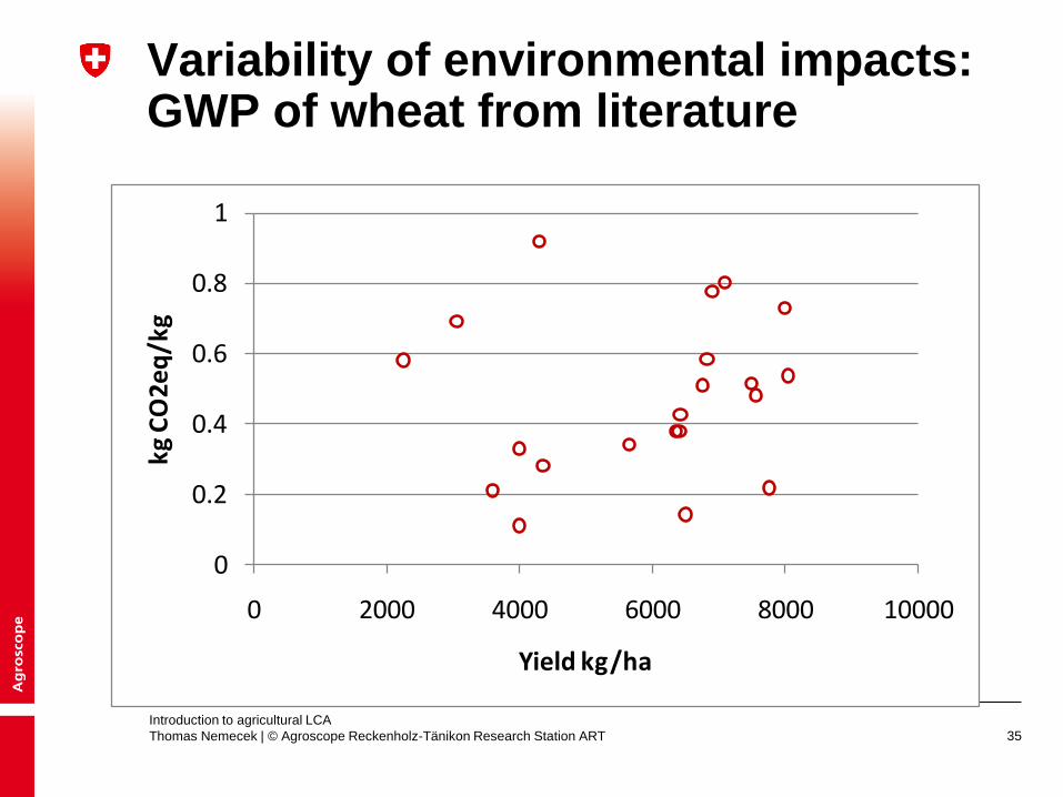
Variability and uncertainty: Factors influencing environmental impacts

Crop

management

Pedo-climatic

conditions

Crop yield

Life cycle

inventory

Environmental

impacts

To understand the

variability of

environmental

impacts, we need to

look on the

variability of the

influencing factors

Socio-economic

conditions

35

Variability of environmental impacts: GWP of wheat from literature



0

0.2

0.4

0.6

0.8

1

0 2000 4000 6000 8000 10000

kg C

O2e

q/k

g

Yield kg/ha

36



Potential use of multivariate statistics in LCA to explain variability

To select proxies, we have to identify similar

datasets

Multivariate statistics (like principal component

analysis, PCA) can be used to show similarities

between environmental impacts

It can be also used to group environmental profiles,

e.g. of crops

Analysis based on a set of midpoint LCIA indicators

In the study applied to crop inventories from

SALCA (Switzerland) and ecoinvent (global)

37



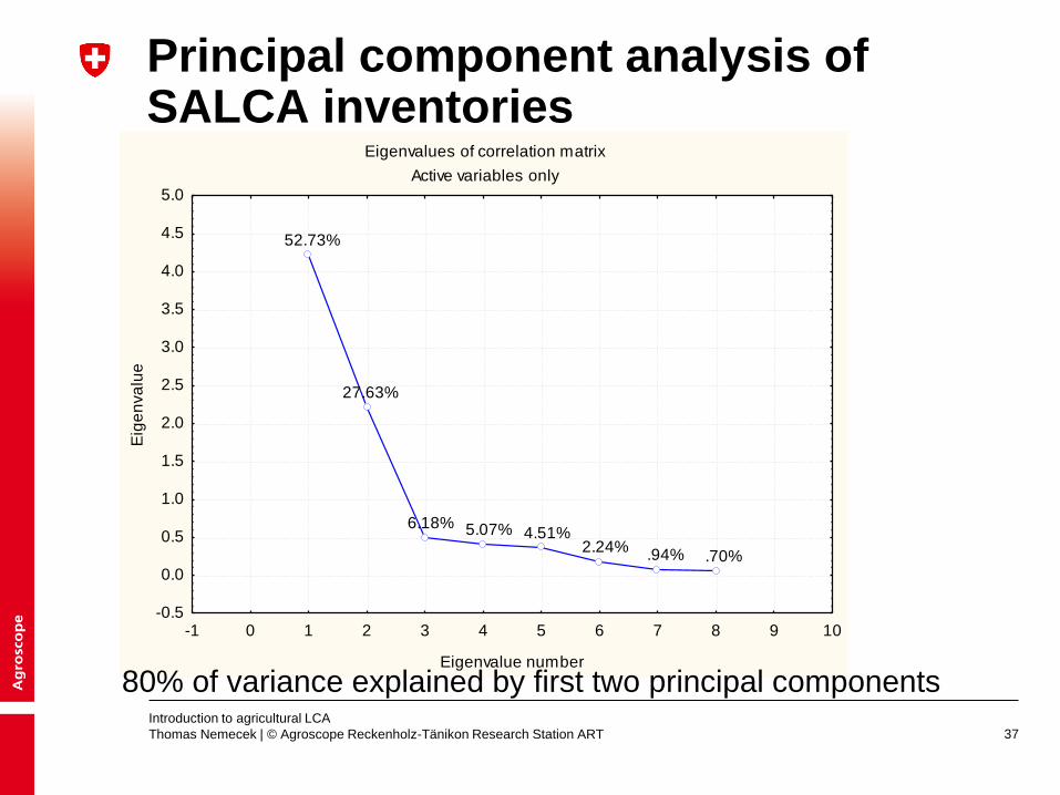
Principal component analysis of SALCA inventories

Eigenvalues of correlation matrix

Active variables only

52.73%

27.63%

6.18% 5.07% 4.51% 2.24%

.94% .70%

-1 0 1 2 3 4 5 6 7 8 9 10

Eigenvalue number

-0.5

0.0

0.5

1.0

1.5

2.0

2.5

3.0

3.5

4.0

4.5

5.0

Eig

en

va

lue

80% of variance explained by first two principal components

38




Relationship between impact indicators and factors 1 and 2

Projection of the variables on the factor-plane ( 1 x 2)

Energy

GWP Ozone

Eutro

Acidi

TET_EDIP

AET_EDIP

HTP_CML

-1.0 -0.5 0.0 0.5 1.0

Factor 1 : 52.73%

-1.0

-0.5

0.0

0.5

1.0

Fa

cto

r 2

: 2

7.6

3%

39



Factor 1: - can group crops - related to the yield

CER

LEG

MAI

OIL

ROOT

VEG-6 -4 -2 0 2 4 6

Factor 1

-4

-3

-2

-1

0

1

2

3

4

5 Data for Swiss crops

from SALCA database:

grouping by crop group

(CER = cereals,

LEG = legumes,

MAI = maize,

OIL = oil crops,

ROOT = root crops,

VEG = vegetables).

Facto

r 2

40



Factor 2: - related to the farming system and the intensity

Conv

Ipint

Ipext

Org-6 -4 -2 0 2 4 6

Factor 1

-4

-3

-2

-1

0

1

2

3

4

5

Data for Swiss crops from

SALCA database: grouping

by farming system

(Conv=conventional,

IPint = integrated intensive,

IPext = integrated extensive,

Org = organic). Facto

r 2

41




Yield is a key factor

Scatterplot (FALSR58_Res 14v*246c)

Factor 1 = -5.9426-2.1271*x

-3.0 -2.8 -2.6 -2.4 -2.2 -2.0 -1.8 -1.6 -1.4 -1.2 -1.0 -0.8 -0.6 -0.4

LnInvYield

-7

-6

-5

-4

-3

-2

-1

0

1

2

Fa

cto

r 1

LnInvYield:Factor 1: r2 = 0.4561

42



Principal component analysis of ecoinvent inventories

Cereals in different countries

w heat

barley

rye

CH

FRES

DE

CH

CH

US

CH

FRES

DE

CH

CH

CH

RER

CH

CH

-8 -6 -4 -2 0 2 4 6

Factor 1

-2

-1

0

1

2

3

43



Potential use of multivariate statistics in LCA to explain variability

Between 76 and 80% of the variability could be explained by the first

two principal components.

Factor 1 crop (group) and yield

Factor 2 farming system (conventional, integrated, extensive,

organic)

More data are needed for more systematic analyses

The analysis helps to

show similarities and differences between environmental profiles

to find suitable proxies

to derive simplified methods for extrapolations and approximations

44



Methodology example 1: Factor analysis Milk production in 35 farms

0.0

0.1

0.2

0.3

0.4

0.5

0.6

0.7

0.8

0.9

1.0

-0.2 0.0 0.2 0.4 0.6 0.8 1.0 1.2

Factor 1

Fa

cto

r 2

Terr.ecotox.

Tot.eutr.Terr.eutr.

Aq.Eutr.

Acid.

Aq.ecotox.

GWP100

GWP500

Ozone

Hum.tox.

Energy

-0.2

0.0

0.2

0.4

0.6

0.8

1.0

-0.2 0.0 0.2 0.4 0.6 0.8 1.0 1.2

Factor 1

Fa

cto

r 3

Terr.ecotox.

Tot.eutr.

Terr.eutr.

Aq.Eutr.

Acid.

Aq.ecotox.

GWP100 GWP500

Ozone

Hum.tox.

Energy

Source: Rossier & Gaillard (2001)

45



1 2 3

No. Impact categories

1 Energy use (GJ eq. ha-1

) 0.95 -0.03 0.06

2 Global warming potential for 100 years (t CO2 eq. ha-1

) 0.95 -0.01 0.20

3 Ozone formation (kg C2H4 eq. ha-1

) 0.94 -0.04 -0.01

4 Aquatic ecotoxicity (kg Zn eq. ha-1

) 0.00 0.93 0.07

5 Terrestrial ecotoxicity (kg Zn eq. ha-1

) 0.07 0.93 0.00

6 Aquatic eutrophication (kg PO4 eq. ha-1

) 0.19 0.05 0.98

7 Terrestrial eutrophication (kg PO4 eq. ha-1

) 0.90 0.13 0.16

8 Acidification (kg SO2 eq. ha-1

) 0.94 0.13 0.16

Total variance explained

Initial eigenvalues 4.58 1.76 0.89

Variance explained (% of variance) 57.19 22.00 11.17

N = 445; loadings exceeding 0.8 are in bold print.

Component

Methodology example 2: Principal component analysis (PCA) 445 apple orchards, Switzerland, 1997-2000

Source: Mouron et al. (2006)

46



Result: The Management triangle

47



Application of the management triangle to the environmental management of farms Example for 35 milk producers, impacts per kg milk Small area = favourable for the environment

Nutrients

Ressources

Pollutants

31 17 32 30 27 10 35

22 24 9 29 23 26 28

19 14 8 3 16 11 13

34 2 12 4 6 15 5

7 1 18 20 25 21 33

Source: Rossier D. & Gaillard G., 2001. Bilan écologique

de l'exploitation agricole: Méthode et application à 50

entre-prises. Rapport SRVA et FAL, 105 pp. et annexes.

48



Environmental management of apple orchards Input-impact-map: correlations between selected impacts and input groups 445 apple orchards, Switzerland, 1997-2000; Pearson correlation (r)

0.0

0.2

0.4

0.6

0.8Diesel

Equipment

Buildings

Tractors

Hail protection

Ca- and Mg-fertilizer

N-fertilizer Other plant treatment

products

K-fertilizer

Fungicides

Insecticides

Herbicides

P-fertilizer

Energy use (GJ eq. ha-1)

Aquatic ecotoxicity (kg Zn eq. ha-1)

Aquatic eutrophication (kg PO4 eq. ha-1)

Energy demand

correlated to 8 of 13

inputs.

Aq. ecotox. determined

by insecticides (0.7) and

fungicides (0.5).

Aq. eutrophication

depends on P-fertiliser

(0.8) and N-fertiliser

(0.4).

Source: Mouron et al. (2006)

49



Conclusions multivariate analysis

Midpoint impact indicators can be grouped by

multivariate statistical methods

Three dimensions were derived for farming systems:

Resource management

Nutrient management

Pollutant management

Related to

Different environmental impacts

Different management options

Different time scales

Enables improved management and communication

50

Global warming potential of dairy farms and amount of milk produced



0.0

0.5

1.0

1.5

2.0

2.5

0 100'000 200'000 300'000 400'000 500'000

kg C

O2

-Eq

./kg

milk

Amount of milk produced (kg/year)

51

GWP of milk processed in dairies



0

0.02

0.04

0.06

0.08

0.1

0.12

0.14

0.16

0.18

0.0E+00 1.0E+07 2.0E+07 3.0E+07 4.0E+07

CO

2-e

q/k

g m

ilk p

roce

sse

d

Milk processed (kg)

52

GWP and dairy size



All

0.0

-1.0

Mio

. kg

1.0

-1.5

Mio

. kg

1.5

-2.0

Mio

. kg

2-3

Mio

. kg

3-5

Mio

. kg

5-1

0 M

io.

kg

>1

0 M

io.

kg milk processed

0.00

0.02

0.04

0.06

0.08

0.10

0.12

0.14

0.16

0.18kg

CO

2e

q/k

g m

ilk p

roce

sse

d

53

Communication of results to farmers Overview of environmental impacts

Environmental impacts per ha UAA

0%

20%

40%

60%

80%

100%

120%

140%

160%

180%

200% ow n farm

model farm

terrestrial ecotoxicity

(Toxp./ha)

aquatic ecotoxicity

(Toxp./ha)

energy demand (MJ-eq./ha)

global w arming

potential (CO2-

eq./ha)

eutrophication (N-

eq./ha)

Environmental impacts per Swiss-Fr. return

0%

20%

40%

60%

80%

100%

120%

140%

160%

180%

200%

ow n farm

model farm


(Toxp./Fr.)

global w arming

potential (CO2-eq./

Fr.)

aquatic ecotoxicity

(Toxp./ Fr.)

energy demand (MJ-eq./ Fr.)

eutrophication

N-eq. / Fr. RL

Environmental impact per MJ digestible energy

0%

20%

40%

60%

80%

100%

120%

140%

160%

180%

200%ow n farm

model farm


(Toxp./MJ DE)

aquatic ecotoxicity

(Toxp./MJ DE)

energy demand (MJ-eq./MJ DE)

global w arming

potential (CO2-

eq./MJ DE)

eutrophication (N-

eq./MJ DE)



54

Communication of results to farmers Detailed environmental impacts

Share of the different means of production in the total energy demand

0

200000

400000

600000

800000

1000000

1200000

1400000

ow n farm model farm

MJ-e

q.

Other inputs

Animal husbandry

Animals (purchase)

Pesticides

Machines

Bulidings/facilities

Feedstuff (purchase)

Energy carriers

Fertilisation/Nutrients



55

Communication of results to farmers Environmental impacts by product group

Environmental impact cowmilk

0%

20%

40%

60%

80%

100%

120%

140%

160%

180%

200%

ow n farm

model farm

energy demand MJ-eq/ha

global warming

potential CO2-eq./ha

eutrophication N-eq./haaquatic ecotoxicity Toxp./ha


Toxp./ha

Environmental impacts cattle breeding

0%

20%

40%

60%

80%

100%

120%

140%

160%

180%

200%

ow n farm

model farm

energy demand MJ-eq./ha

global w arming

potential CO2-

eq./ha

eutrophication

N-eq./ha

aquatic ecotoxicity

Toxp./ha


Toxp./ha



56

Communication of results to farmers Comparison to similar farms

Energy demand: comparison of dairy farms

0

10000

20000

30000

40000

50000

60000

70000

80000

1 2 3 4 5 6 7 8 9 10 11 12 13 14

MJ

-eq

. /h

a

Other inputs

Animal husbandry

Animal (purchase)

Pesticides

Machines



Energy carriers


Eutrophication: comparison of dairy farms

0

50

100

150

200

250

300

350

1 3 9 2 12 8 10 5 13 11 4 6 7 14

N-e

q.

/ha

Other inputs

Animal husbandry

Animal (purchase)

Pesticides

Machines



Energy carriers




57

Milk production Energy demand of specialised milk production farms

0

10000

20000

30000

40000

50000

60000

70000

80000

90000

1 3 5 7 9 11 13 15 17 19 21 23 25 27 29 31 33

MJ-é

q./

ha S

AU

*an

Autres intrants

Animaux (achats)

Fourrages (achats)

Semences (achats)

Produits phytosanitaires

Engrais

Agents énergétiques

Machines

Bâtiments/ équipements



58

Milk production Energy demand of specialised milk production farms

44%

0%3%

11%

19%

17%

0%

6%

Agents énergétiques

Semences (achats)

Fourrages (achats)

Animaux (achats)

Bâtiments/ équipements

Machines

Engrais

Produits phytosanitaires

Autres intrants

Infrastructure &

intrants industriels

33%

Consommation directe

44%

Intrants agricoles

23%



59

Conclusions

The environmental impacts of agriculture and the food sector

are considerable

Agriculture has a number of specific aspects that need to be

considered

LCA provides good insights into the behaviour of the systems

For this a close collaboration between agronomists,

environmental scientists and local experts is required



agroscope reckenholz-tänikon research station art · pdf fileagroscope...

Documents