hydrogeological modeling to support the … · also, i would like to thank dr. ignaz buerge from...
TRANSCRIPT

SCUOLA DI DOTTORATO
UNIVERSITÀ DEGLI STUDI DI MILANO-BICOCCA
Department of Earth and Environmental Sciences (DISAT)
PhD program in Chemical, Geological and Environmental Sciences
Cycle XXX
Curriculum in Environmental Sciences
HYDROGEOLOGICAL MODELING TO
SUPPORT THE MANAGEMENT OF
GROUNDWATER RESOURCES IN
ALPINE VALLEYS
Surname Stefania
Name Gennaro Alberto
Registration number 759627
Tutor: Prof. Bonomi Tullia Supervisor: Dr. Rotiroti Marco
Coordinator: Prof. Frezzotti Maria Luce
ACADEMIC YEAR 2016/2017


Index
i
Index
Abstract _____________________________________________________________ ii
Acknowledgments _____________________________________________________ iii
1. Introduction ______________________________________________________ 1
2. Aims of PhD project _________________________________________________ 2
3. Study area _______________________________________________________ 18
4. Thesis structure ___________________________________________________ 20
4.1. Groundwater/surface-water interaction modeling ________________________ 20
4.2. Hydrochemical data management ___________________________________ 21
4.3. A methodology to define landfill trigger levels ___________________________ 23
4.4. Identification of groundwater pollution sources in a landfill site _______________ 24
5. Publications ______________________________________________________ 26
5.1. Modeling groundwater/surface-water interactions in an alpine valley (the aosta plain, nw italy): the effect of groundwater abstraction on surface-water resources __________ 27
5.2. The hydrochemical database tangchim, a tool to manage groundwater quality data: the case study of a leachate plume from a dumping area _______________________ 62
5.3. Determination of trigger levels for groundwater quality in landfills located in historically human-impacted areas ______________________________________ 78
5.4. Identification of groundwater pollution sources in a landfill site using artificial sweeteners, multivariate analysis and transport modeling ______________________ 97
6. Conclusions _____________________________________________________ 133
7. Future developments _______________________________________________ 139
8. Articles and presentation ____________________________________________ 141

Abstract
ii
Abstract
The present PhD project deals with the development of methodologies and tools in order to support
the management of groundwater resources from a quantitative and qualitative point of view. The
work deals with a particular hydrogeological context such as the Alpine valleys aquifers, where
groundwater/surface water interactions as well the wells pumping have a crucial role in the
hydraulic behaviour of groundwater. Moreover, the hydrogeological setting of these aquifers
makes groundwater highly vulnerable to the contamination by the human activities.
The work involves three main topics concerning specified issues affecting the Alpine valley aquifer
of the Aosta Plain (Aosta Valley Region, N Italy).
The first topic is related to the modeling of the three-dimensional groundwater flow and its
interaction with the surface water. This topic was addressed by the development of a numerical
groundwater flow model of the Aosta Plain aquifer in order to identify groundwater/surface-
water relationships and evaluate the overall effect of the pumping on water resources. The model
was developed using MODFLOW2005 and the more recent Stream-Flow routine package (SFR2)
to simulate the surface-water network. An inverse calibration procedure performed by the PEST
code was used to obtain the steady-state and transient solutions. The quantification of the
hydrogeological budget, the groundwater/surface-water interactions and the effect of well
withdrawals on water resources were done using the model results.
The second topic deals with the management of groundwater hydrochemical data. This topic was
addressed through the development of the online hydrochemical database called TANGCHIM
which was joined with an existing hydrogeological database in order to provide an integrated
platform able to manage, display and share water quality and quantity data.
The third topic takes into account a groundwater pollution related to a landfill site. Within this
topic, two main aims were achieved. The first one is related to the definition of a methodology able
to support groundwater managers to define the conceptual model of the site and to calculate the
trigger levels as useful tool for monitoring landfill sites located in historical human-impacted
areas. The second aim is related to the detection of the sources related to the groundwater
contamination affecting the landfill site. The investigation was conducted using hydrochemical
parameters, artificial sweeteners as tracers, multivariate statistical analysis and transport
modeling. The source apportionment analysis was accomplished to distinguish the contribution of
different sources of the leachate infiltration in order to improve the management of the landfill site
and design a proper remediation system.

Acknowledgments
iii
Acknowledgments
First and foremost, I want to thank my tutor, Prof. Tullia Bonomi for the opportunity of this PhD. I
really appreciated all her knowledge, ideas, continuous support and motivation to make my PhD
experience productive and stimulating. I am also thankful for the excellent example she has provided
as a person and professor. I would like to thank my supervisor Dr. Marco Rotiroti for the professional
support, good advice and collaboration, especially during my research and writing papers. My
sincere thanks goes to Dr. Letizia Fumagalli for her precious comments and suggestions.
I would like to thank ARPA Valle d’Aosta in the persons of Pietro Capodaglio and Fulvio Simonetto
for the opportunity of this PhD project.
I would like to thank the laboratories of DISAT, in particular Dr. Barbara Leoni, Prof. Antonio
Finizio, Dr. Valentina Soler and Dr. Sara Villa for providing hydrochemical and sucralose analysis.
Also, I would like to thank Dr. Ignaz Buerge from Swiss Federal Research Station (Agroscope) for
providing artificial sweeteners analysis of groundwater and surface water samples.
I would like to thank my friend and PhD student Chiara Zanotti for all the desperation and fun we
have shared in the last three years. My sincere thanks also go to Dr. Sara Taviani for the contagious
passion for our work.
I would like to thank my family for supporting me unconditionally throughout my life.
And most of all, I would like to thank my partner Mari for all her love, continuous support and
encouragement throughout this PhD and our life. Thank you.

1. Introduction
1
1. Introduction
Water is a fundamental resource to preserve the life on the Earth. Its availability, in terms of quantity
and quality, is at the same time a growth and limiting factor widely considered in the evolution of
the human history. It was estimated that the total amount of water on the Earth is about 1 billion and
386 million km3 of which about only 35 million is freshwater. The 68.7% of the freshwater is not
available for the use since it is stored in glaciers and snow cover. Instead, the total available
freshwater is about 30.37% of which groundwater represents the 30.1% whereas surface-water is
about 0.27% (Shiklomanov, 1993).
Bringing in mind the relative availability in many areas of the planet, the low cost related to the well
pumping, groundwater has acquired a key role on the human water supply and it has become the
main water resource used for humans needs. However, in the more recent past, the industrialization
processes have induced an increase both of population and human needs followed by a sharply
increase of groundwater exploitation due to the well pumping and groundwater pollution due to
direct/indirect infiltration of contaminants from waste, industry, agriculture, drugs and any other
activity (Sophocleous, 2000).
Despite its significant advantages, groundwater is not an unlimited resource and its recovery time in
the case of overexploitation and pollution problems could be decades and centuries, respectively
(LHM et al., 1991). As a consequence, in the last decades, researchers and stakeholders have paid
more attention to overexploitation, depletion and pollution problems affecting groundwater
resources.
The protection of the water resources is one of the cornerstones of environmental protection in
Europe. The EU directives 2000/60/CE (EC, 2000) and 2006/118/CE (EC, 2006), established a
framework for Community action in the field of water policy, in particular on the protection of
groundwater against depletion, pollution and deterioration, so protecting both quantity and quality
of groundwater. Accordingly, groundwater management is an arduous challenge, since it should
sustain, over the long term, the hydrogeological equilibrium, in particular between different
interconnected water bodies and human supply. At the same time, many efforts should be spent in
order to guarantee a good quality status of groundwater that is continuously threatened by human
contamination.

2. Aims of PhD project
2
2. Aims of PhD project
The main aim of the present project is to apply the academic research on the management of the
groundwater resource. In particular, this work deal with the development of tools and strategies to
support the management of the groundwater resource in order to ensure the preservation of its
quantitative and qualitative status over the time.
The present PhD work involves three main general topics each of which developed on specified issues
affecting the Alpine valley aquifer of the Aosta Plain. In particular:
I) Groundwater/surface water interaction. This topic was addressed by the
development of the groundwater flow model of the Aosta Plain aquifer in order to identify
groundwater/surface-water relationships and evaluate the overall effect of well pumping on
water resources;
II) Hydrochemical data management. This topic was addressed through the development
of the hydrochemical database called TANGCHIM which was joined with an existing
hydrogeological database in order to provide an integrated platform able to manage, display
and share water quality and quantity data;
III) Landfill impact on groundwater quality. This topic was addressed by combining the
use of multivariate statistical analysis, emerging tracers (i.e. artificial sweeteners) and
modeling approaches in order to obtain: the conceptual model of the groundwater
contamination related to a landfill site located within the Aosta Plain, methodologies for its
monitoring and the identification of the groundwater pollution sources in the landfill site.
The present PhD project arises from the collaboration between the Regional Environmental
Protection Agency of the Aosta Valley Region (ARPA VdA) and the Department of Earth and
Environmental Sciences of the University of Milano-Bicocca.

2. Aims of PhD project
3
Groundwater/surface-water interaction In natural condition, the recharge and discharge of an aquifer are balanced, however, the human
groundwater exploitation can affect this equilibrium.
In particular for groundwater/surface-water interconnected systems, wells pumping can increase
the amount of the outflow discharged from an aquifer inducing both a decrease of the groundwater
availability and rivers depletion, especially in the dry season when the streamflow is mainly
constituted by the base flow component (Feinstein, 2012). Indeed, rivers are commonly the primary
receptors of groundwater discharge and the latter is often the primary component of river discharge
as base flow. As a consequence, the evaluation of the interactions between groundwater and surface-
water, taking also into account the effect of wells pumping, should be mandatory, however, it is still
challenging for hydrogeologists. (Alley et al., 2007; Zhou, 2009).
In this context, the storage capability of the aquifer plays a key role. Indeed, the initial water pumped
by a well comes from the water stored in the aquifer (Sanz et al., 2011) and the release of this water
continues until the well capture zone reaches another more accessible water. This water abstraction
can originate a reduction of the natural outflow of the aquifer or an increase of the natural or artificial
inflow to the aquifer from other connected water bodies. In the first case, the pumping subtracts
water that, otherwise, would have flowed to other interconnected systems (e.g. river, pound,
wetland). In the second case, the pumping can induce a water leakage from the connected surface-
water bodies up to invert the type of existing relationship between them, especially in the case of a
gaining river (Fetter, 2001). The above-mentioned behaviours induced by pumping results in
streamflow depletion and/or groundwater overexploitation.
The effect of the well pumping is quite fast on groundwater rather than on surface-water where it
may be evident only many years after pumping begins (Barlow and Leake, 2012). River discharge
depletion due to pumping has to become an important water-resource management issue since these
negative impacts may affect the aquatic system, surface-water availability and the quality and
aesthetic values of the rivers.
Many different approaches based on hydrochemical, hydrogeological and numerical modeling can
be used to investigate groundwater and surface-water interactions. The first two mentioned
approaches include methodologies based on heat tracers, hydrochemical tracers, isotopes, mixing
models, mass balance approaches and Darcy’s law (i.e. study of the hydraulic gradient), nevertheless
more reliable results arise only by the combined use of more than one of the previously listed
methods (Mencio´ et al., 2014). These methodologies may help to depict the whole complexity of the
groundwater/surface-water interactions. However, since they neglect the pumping effects and they
are unable to consider the transient conditions occurring within an aquifer, the possibility to evaluate

2. Aims of PhD project
4
the impact of well pumping over the time, in terms of groundwater overexploitation and river
depletion on the water resources, is prevented.
On the contrary, the numerical modeling approach provides powerful tools for quantifying the effects
of the well pumping on both groundwater and surface-water, allowing to of well abstraction,
groundwater exploitation and river depletion.
The numerical groundwater models can be developed and solved through two main approaches
which are the finite difference method (FDM) and the finite element method (FEM).
The FDM leaves the physical model unchanged discretizing the differential equations of the problem
under investigation. Using the FDM the model user establishes a regular grid over the model area
that subdivides the total model area into rectangular subdomains where the differential equations
are solved. Constant system parameters are then assigned to each cell as cell value. Unknown
variables (e.g. hydraulic head for groundwater flow model) are calculated as discrete values at the
grid node or at the central points of the cells (Spitz and Moreno, 1996). The effectiveness of the finite
difference method increases with the increase of the number of the points (where the function is
unknown) on which the related equation is solved. The FDM is able to solve complex problems (for
example Numerical Fluid Dynamics). However, if the geometries of the system become very irregular
or particular boundary conditions occur this method could be challenging to be applied.
The FEM differs from the FDM model by approximating the flow equation through and integration
rather than a differentiation. In the case of FEM, the model area is subdivided into subareas, called
elements, that usually are triangular elements. Since there are basically no restriction on the shape
of the elements, the discretization of the modeled area is more flexible with respect to FDM. The
general approach used by FEM is to approximate the solution of the unknown variable (e.g. hydraulic
head for groundwater flow model) by piecewise linear functions and its distribution is approximated
for each element by a linear function (Spitz and Moreno, 1996). The idea of the approximation used
by the FEM is to approximate the true trend of the unknown function with some other functions of
which the trend is known.
The two main codes used to develop three-dimensional groundwater flow models are MODFLOW
and FEFLOW. MODFLOW is a free code developed by U. S. Geological Service. It is a FDM modular
code able to simulate the groundwater flow within the aquifer using a block-centered finite-
difference approach. MODFLOW code have a modular structure that consists of a main program and
a series of highly independent "packages." Each package deals with a specific feature of the
hydrologic system which is simulated. The division of the program into modules permits the user to
examine specific hydrologic features of the model independently. This also facilitates the
development of additional capabilities because new modules or packages can be added to the

2. Aims of PhD project
5
program without modifying the existing modules or packages (Harbaugh, 2005; Harbaugh et al.,
2000; McDonald and Harbaugh, 1984).
FEFLOW is a proprietary and not freely available FEM code which uses a finite element (triangular)
mesh to represent the model domain. The triangular mesh can be more easily adapted to variable
stratigraphy such as sloping or pinch outs, and allows for versatile discretization of non-rectangular
model domains (Trefry and Muffels, 2007).
The FEFLOW provides a better representation of anisotropy since it is based on FEM where each
node which composes a triangular element of the mesh have own coordinates. Conversely,
MODFLOW is based on a regular grid composed of regular cells on which the distribution of the
aquifer propriety and the solution of the groundwater flow equation is discretized. However, the use
of a code based on FEM does not guarantee the local mass conservation and there can be some
discontinuous velocities at the element boundaries. Lastly, FEFLOW uses more generic boundary
conditions to simulate different elements of the hydrogeological system (e.g., river, drain, well, no-
flow zone, etc.).
The MOFLOW code is an international standard used by hydrogeologists to develop groundwater
flow model. The main advantage of the MODFLOW code is that the obtained solution is mass
conservative, accordingly, the analysis of the groundwater mass-balance computed by the code is
more reliable. Moreover, as stated above, MODFLOW uses various packages to simulate different
elements of the hydrogeological system.
In this context, surface-water can be simulated by using many types of boundary conditions and
packages (e.g. GHB, RIV, STR, SFR2, Lake). Unfortunately, in order to understand the relationships
between groundwater/surface-water, too simple and not specific boundary conditions are often used
to simulate surface-water. This leads to an over-simplification of the dynamics occurring between
groundwater/surface-water and wells pumping, limiting the model capability to understand their
complex dynamics. In order to overcome this limitation, the Streamflow Routing (SFR2) Package
(Niswonger and Prudic, 2000, 2010) can be used. In particular, SFR2 is able to compute and
simulate the streamflow and stage of the river. So, using SFR2 water capture by pumping wells can
make river segments dried or change the direction of the water exchange, gaining and losing river
segments can be identified, river segment behaviour can respond to water-table oscillation, surface-
water diversions can be simulated and unsaturated flow between river and aquifer can be computed.
Furthermore, the implementation of numerical models to manage aquifers system also provides the
possibility to evaluate many other aspects related to groundwater. For example, the MODPATH code
(Pollock, 2012) allows to track the advective component of the groundwater flow, whereas the

2. Aims of PhD project
6
MT3DMS code (Zheng, 2010; Zheng and Wang, 1998) is able to simulate the fate of dissolved
contaminants taking into account the advective-dispersive transport equation using the MODFLOW
solution as a basis for groundwater flow.
The use of numerical modeling allows to consider, at the same time, different aspects that could have
different weights on the evaluation of the quantity and quality status of the groundwater resource.
Overall, groundwater model provides the chance, on one hand, to improve the comprehension of the
behaviour of the system and, on the other hand, to implement more suitable management policies
for the groundwater resource.
In the present PhD project, this topic was addressed by developing a three-dimensional numerical
groundwater flow model of the Aosta Plain through the use of the SFR2 Package and MODFLOW
2005.

2. Aims of PhD project
7
Hydrochemical data management
Groundwater is often felt as a relatively stable and well-protected water resource. However, a safe
drinking water supply from groundwater is a complex task to assure. The understanding of the
hydrological systems and the processes of pollutant transport is the basis of an efficient water
management. This process should be based on the observations and scientific interpretation of the
data collected in the field.
In order to do that, it could be possible to integrate tools and methodologies into informatic systems
developed to manage field data stored in specified and well-structured database, providing outcomes
for the water managers in an easily understandable and usable form. The integration of database and
tools forms a decision support system (DSS) (Janža, 2015).
A DSS is a computer-based system that uses data stored in a connected and specific database, aiding
the process of decision making (Sprague Jr and Carlson, 1982). Moreover, DSS utilizes data and
models to solve unstructured problems in order to help decision makers (Finlay, 1994; Power, 2004).
Considering the above definitions, DSS ranges from systems answering of simple queries to systems
modeling of a complex human decision-making process (Nizetic et al., 2007).
In the context of groundwater resources, DSSs are often used to facilitate groundwater management
in terms of suitable exploitation of the resources and to optimize groundwater remediation. Different
examples of DDS are shown in literature. As for the quality management of groundwater, Track et
al. (2008) developed a groundwater management tool coupled with an early warning system aimed
at managing and controlling hazardous compounds in groundwater catchment areas. Ertel and
Kirchholtes (2007) developed a tool focused on the optimization, evaluation and management of
contaminated groundwater in urban area based on the cycling screening of groundwater
hydrochemical data. Janža (2015) described a DSS for emergency groundwater management that
was developed to improve activities after the discovery of pollution. The DSS is composed of a user-
friendly graphical interface that enables water managers to utilize the database, numerical modeling
techniques and expert knowledge, and thus gives them fast and easy access to supporting
information for mitigating groundwater pollution.
As shown before, DSSs requires to implement at least one database that allows to store data. This
database is the core of a DSS because it represents the source of data for all implemented tools. For
this reason, the design of the structure and capabilities of the database represents an important
task during a DSS developing.

2. Aims of PhD project
8
In order to investigate and manage aquifer systems and groundwater contamination events, both
new and historical hydrogeological and hydrochemical data have to be collect from fields surveys,
institutional monitoring networks and well-drilling cores. However, these data are often difficult to
obtain and share because they are managed by different public and/or private operators who store
data in different formats and on different information supports. Moreover, databases are often
designed each time as a simple “tank” for a specific project or specific study area.
Usually, hydrochemical databases are more difficult to manage with respect to the hydrogeological
database. Indeed, in many cases, the number of the analysed chemical compounds and the
groundwater sampling frequency are much higher than hydrological data. Besides, the name of a
chemical compound can have more than one synonymous jeopardizing the integrity of the dataset
by means of lack or duplication of data. As a consequence, many resources have to be spent to design,
compile and join data from different sources in a new specific database. Moreover, this process, if
not properly managed, could lead to redundancy as far to leak of data.
As stated before, both hydrogeological and hydrochemical data have to be considered in order to
properly manage the groundwater resources. Moreover, it is desirable that these data can be easily
recovered, used and shared. For this reason, an ever-increasing need in developing online integrated
platforms is felt, in order to store, display and process different kinds of groundwater data. These
online platforms, being easily accessible, could be used as a base to integrate tools or procedures able
to analyse available data and providing a support system to decision-makers or scientists for a more
effectiveness management and comprehension of water resources.
This topic was addressed in the PhD project by developing the on-line hydrochemical database called
TANGCHIM.

2. Aims of PhD project
9
Landfill impact on groundwater quality
Groundwater pollution is another key aspect that must be managed in order to guarantee the good
quality status of groundwater. In this light, wastes represent one of the most important threats for
groundwater quality, since they can contain a wide range of pollutants (Christensen et al., 2001; Han
et al., 2013). Accordingly, quite some groundwater contamination events caused by leaks of leachate
from landfills have been reported in literature (Christensen et al., 1998; Fatta et al., 1999; Giusti,
2009; Han et al., 2013, 2016; Laner et al., 2012; Lyngkilde and Christensen, 1992; Mor et al., 2006;
Öman and Junestedt, 2008).
Especially in the past, wastes were disposed in the environment without paying any attention to
probable leachate infiltrations toward soil and groundwater, building over the time many
uncontrolled and unlined landfills that caused groundwater pollution. The environmental regulation
partially reduced the uncontrolled disposal of waste by calling for rigorous prescriptions, such as a
lined system able to avoid leaks and percolation of pollutants through soil and groundwater (Read
et al., 2001).
As regards of the waste management, nowadays, the European legislative referent is the 99/31/EC
Landfill Directive (EC, 1999) that aims to prevent or reduce the negative effects of landfills on soils,
surface-water and groundwater. It establishes a list of requirements for a proper groundwater
monitoring network in landfill sites and specifically imposes the definition of trigger levels to identify
significant adverse environmental effects on groundwater, of course on the basis of a proper
conceptual model of the site. As regards of the trigger level, the Directive provides a general guideline
for their determination related to new landfills built in an unpolluted site, whereas no methodologies
are suggested for landfills built in historically human-impacted areas.
In order to evaluate the impact of human activities on the quality of groundwater and surface-water,
recent studies have paid attention to the use of new emergent contaminants, tracers and isotopes
(Buerge et al., 2011; Clarke et al., 2015; Eggen et al., 2010; Lapworth et al., 2012, Sui et al., 2015, Van
Stempvoort et al., 2011). Water, nitrogen and carbon isotopes are well-known robust tracers typically
used to depict the evolution of groundwater contamination related to leachate plume originate by
landfills, septic tank, etc. (Caschetto et al., 2018; Van Breukelen et al., 2003). Although isotopes are
considered robust tracers, they have high costs related to sampling and analysis.
Lange et al. (2012) found that the artificial sweeteners can be considered a new class of emerging
traces in groundwater, since they are conservative and they were found in groundwater affected by
leachate plume and sewage (Buerge et al., 2009; Lange et al., 2012; Van Stempvoort et al., 2011).
Artificial sweeteners are usually used as sugar substitutes in foods, beverages, drugs and sanitary
products. A Canadian study reported the use of different types of artificial sweeteners, selected on
the basis of their approval and following introduction as a product additives, to trace leachate plumes

2. Aims of PhD project
10
originated from different landfills (Roy et al., 2014), highlighting the possibility of using these
compounds to trace different leachate plumes on the basis of the landfill age.
Broadly speaking, many works, regarding groundwater impacted by leachate plumes, focused on the
description of the overall composition and behaviour of the groundwater leachate plume (Bjerg et
al., 1995; Clarke et al., 2015; Cozzarelli et al., 2011a; Han et al., 2016). Christensen et al. (2001)
summarizing the main involved processes governing contaminants in leachate affected aquifer such
as dilution, sorption, ion exchange, precipitation, redox reactions and degradation. The authors
underlined that the redox-processes and the related zonation always occur in a groundwater leachate
plume. For this reason, the comprehension of the redox zone distribution is an important task to
understand. Moreover, the contaminants patterns in a leachate plume change as the leachate
migrates away from landfill. These process are promoted by microbial communities (Christensen et
al., 1998) that use the dissolved organic carbon, that composes the leachate (Fatta et al., 1999; Mor
et al., 2006), as substrate to maintain the microbial redox processes (Ludvigsen et al., 1998).
Although the COD is usually monitored in landfill site to evaluate the likely infiltration in
groundwater of leachate, and thus organic matter, its content is also affected by other reduced
species like Fe, Mn or H2S that can significantly contribute to it. More reliable indicators of the
presence of organic carbon in groundwater which could be considered when studies are focused on
the redox-zonation of a leachate plume are DOC (Dissolved Organic Carbon) or TOC (Total Organic
Carbon) because their quantification are not affected by the presence of redox-sensitive species.
Moreover, the DOC coupled with other tracers could allow to trace both the evolution of the oxidation
of dissolved organic carbon and the three-dimensional extension of a landfill leachate plume (van
Breukelen et al., 2003, Cozzarelli et al 2011). For this reason, the DOC or TOC detection should have
to be imposed for the groundwater monitoring nearby landfill site by regulation, instead of COD.
A good characterization of a plume should consider the vertical quantification of the investigated
contaminants, especially for the redox-sensitive species such as O2, Fe, Mn, As, NH4, etc (Colombani
et al., 2015). This need arises from the evidence that water-quality samples collected from long-
screen wells may be not representative of the quality of the water in the aquifer because of the vertical
flows of water in the well induced by pumping. Vertical flows in a well can be increased by: high
aquifer transmissivity, greater proximity to discharge or recharge zone, greater well volume and
greater vertical/horizontal anisotropy (McMillan et al. 2014). In these cases, the water origin of the
sample is sensitive to pump intake position, pumping rate and pumping duration. Furthermore,
McMillan et al. (2014) showed that when vertical gradients are present, a sample bias is present even
when the local vertical flow in the wellbore is less that the pumping rate. Appelo and Postma (2004)
clarified the effect of the water mixing on a typical redox-species such as Fe2+ on a fully completed
well, sampled without using multi-level methods. They have shown a typical vertical profile of Fe2+

2. Aims of PhD project
11
and O2 in a sandy aquifer obtained by depth-specific sampling where a well-defined oxic zone is on
top of an anoxic zone containing Fe2+. The authors stated that if a piezometer fully screened is used,
the obtained water sample will be representative of a mixing of both oxic and anoxic zone.
Furthermore, the oxic water will react with the Fe2+ containing water and the concentrations of O2
and Fe2+ will result alter. This behaviour induces as a result that the water sample collected without
a multi-level sampling does not properly reflect the real conditions of the aquifer because the mixing
of not contaminated and contaminated water, that originates from different screened portions of the
aquifer, distorts the real concentrations of the investigated compounds (Church and Granato, 1996).
For proper depth-specific sampling, dedicated systems are required. For example, new multiple
nested piezometers or multiple-borehole piezometer may be drilled, otherwise removable packer or
backfill system could be used to seal the borehole between monitoring zones to prevent the unnatural
vertical flow of groundwater and maintain the natural distribution of fluid pressures and chemistry
for existing piezometers (Nielsen, 2005). All of these aspects are abundantly discussed in previous
works that constitute the main references for the geochemical characterization of groundwater and
related pollution (Appelo and Postma, 2004; Christensen et al., 2001; Church and Granato, 1996).
Unfortunately, the multi-level sampling is not a widespread practice, especially for the routine
monitoring done by both managers of contaminated-site and environmental control agencies.
Indeed, a multi-level sampling would sharply increase the cost of the monitoring.
Furthermore, neither European or extra-European legislations require multi-level sampling,
therefore both managers and control agencies, in their ordinary activities, usually neglect the vertical
sampling. On this basis, it is required to find and develop tools and methods to effectively use
available data from routine monitoring.
Groundwater affected by the landfill leachate plume is a crucial issue for a safe drinking supply.
Consequently, in these cases one of the most important tasks to properly design a remediation
system is the identification and quantification of the points from which leachate infiltrates toward
underlying aquifer. In order to support the identification of the sources, statistical methods,
modeling and emerging tracers can be used. Usually they are used in a separate way. However, the
combined use of the above mentioned tools could improve and increase the reliability on the
identification of the likely position where the infiltration of pollutant (e.g. leachate) is occurring.
In a landfill site, leaks of leachate could be related, for examples, to a deficiency of the landfill liner
systems, to problems with the leachate collection system or to a previous landfill built in the same
area with no environmental prescriptions. Accordingly, the location of the pollution sources should
be correctly recognized.
2. Aims of PhD project
12
Indeed, inadequate knowledge regarding groundwater pollution sources either leads to decrease the
efficiency of remediation strategies or increase the remediation costs. Therefore, the detection of the
exact sources of the groundwater pollution is a critical issue in groundwater management. Thus, the
estimation of the pollution source characteristics including numbers, locations, and release histories
becomes a key task for efficiently managing the groundwater systems and polluted sites (Ayvaz,
2010).
This topic was addressed in the present PhD project using different approaches in order to define
the conceptual model of pollution, a methodology to calculate trigger levels and the identification of
the sources of leachate infiltration in a landfill site affecting the Aosta Plain aquifer.

2. Aims of PhD project
13
References
Alley, W.M., Survey, U.S.G., Alley, W.M., 2007. Another Water Budget Myth: The Significance of
Recoverable Ground Water in Storage. doi:10.1111/j.1745-6584.2006.00274.x
Appelo, C.A.J., Postma, D., 2004. Geochemistry, groundwater and pollution. CRC press.
Ayvaz, M.T., 2010. A linked simulation – optimization model for solving the unknown groundwater
pollution source identification problems. J. Contam. Hydrol. 117, 46–59.
doi:10.1016/j.jconhyd.2010.06.004
Bjerg, P.L., Ruegge, K., Pedersen, J.K., Christensen, T.H., 1995. Distribution of redox-sensitive
groundwater quality parameters downgradient of a landfill (Grindsted, Denmark). Environ. Sci.
Technol. 29, 1387–94. doi:10.1021/es00005a035
Buerge, I.J., Buser, H.R., Kahle, M., Müller, M.D., Poiger, T., 2009. Ubiquitous occurrence of the
artificial sweetener acesulfame in the aquatic environment: An ideal chemical marker of
domestic wastewater in groundwater. Environ. Sci. Technol. 43, 4381–4385.
doi:10.1021/es900126x
Buerge, I.J., Keller, M., Buser, H.R., Müller, M.D., Poiger, T., 2011. Saccharin and other artificial
sweeteners in soils: Estimated inputs from agriculture and households, degradation, and
leaching to groundwater. Environ. Sci. Technol. 45, 615–621. doi:10.1021/es1031272
Caschetto, M., Robertson, W., Petitta, M., Aravena, R., 2018. Partial nitrification enhances natural
attenuation of nitrogen in a septic system plume. Sci. Total Environ. 625, 801–808.
Christensen, J.B., Jensen, D.L., GrØn, C., Filip, Z., Christensen, T.H., 1998. Characterization of the
dissolved organic carbon in landfill leachate-polluted groundwater. Water Res. 32, 125–135.
doi:10.1016/S0043-1354(97)00202-9
Christensen, T.H., Kjeldsen, P., Bjerg, P.L., Jensen, D.L., Christensen, J.B., Baun, A., Albrechtsen,
H.J., Heron, G., 2001. Biogeochemistry of landfill leachate plumes. Appl. Geochemistry 16,
659–718. doi:10.1016/S0883-2927(00)00082-2
Church, P.E., Granato, G.E., 1996. Bias in ground-water data caused by well-bore flow in long-screen
wells. Ground Water. doi:10.1111/j.1745-6584.1996.tb01886.x
Clarke, B.O., Anumol, T., Barlaz, M., Snyder, S.A., 2015. Investigating landfill leachate as a source of
trace organic pollutants. Chemosphere 127, 269–275. doi:10.1016/j.chemosphere.2015.02.030
Colombani, N., Mastrocicco, M., Prommer, H., Sbarbati, C., Petitta, M., 2015. Fate of arsenic,
phosphate and ammonium plumes in a coastal aquifer affected by saltwater intrusion. J.
Contam. Hydrol. 179, 116–131. doi:10.1016/j.jconhyd.2015.06.003
Cozzarelli, I.M., Bohlke, J.K., Masoner, J., Breit, G.N., Lorah, M.M., Tuttle, M.L.W., Jaeschke, J.B.,
2011. Biogeochemical evolution of a landfill leachate plume, Norman, Oklahoma. Ground Water
49, 663–687. doi:10.1111/j.1745-6584.2010.00792.x
EC, 2006. Directive 2006/118/EC of the European Parliament and of the council of 12 December

2. Aims of PhD project
14
2006 on the protection of groundwater against pollution and deterioration. Off. J. Eur. Union
19, 19–31. doi:http://eur-lex.europa.eu/legal-content/EN/TXT/?uri=CELEX:32006L0118
EC, 2000. Directive 2000/60/EC of the European Parliament and of the Council of 23 October 2000
establishing a framework for Community action in the field of water policy. Off. J. Eur. Parliam.
L327, 1–82. doi:10.1039/ap9842100196
Eggen, T., Moeder, M., Arukwe, A., 2010. Municipal landfill leachates: A significant source for new
and emerging pollutants. Sci. Total Environ. 408, 5147–5157.
doi:10.1016/j.scitotenv.2010.07.049
Ertel, T., Kirchholtes, H.J., 2007. .7: INCORE: Integrated Concept for Groundwater Remediation,
in: Groundwater Science and Policy. pp. 316–341.
Fatta, D., Papadopoulos, A., Loizidou, M., 1999. a Study on the Landfill Leachate and Its Impact on
the. Environ. Geochem. Health 21, 175–190. doi:10.1023/A:1006613530137
Feinstein, D., 2012. Paper Since “ Groundwater and Surface Water – A Single Resource ”: some U .
S . Geological Survey advances in modeling groundwater / surface-water interactions 9–24.
doi:10.7343/AS-001-12-0001
Finlay, P.N., 1994. Introducing decision support systems. Oxford, UK Cambridge, Mass. NCC
Blackwell.
Giusti, L., 2009. A review of waste management practices and their impact on human health. Waste
Manag. 29, 2227–2239. doi:10.1016/j.wasman.2009.03.028
Han, D., Tong, X., Currell, M.J., Cao, G., Jin, M., Tong, C., 2013. Evaluation of the impact of an
uncontrolled landfill on surrounding groundwater quality, Zhoukou, China. J. Geochemical
Explor. 136, 24–39. doi:10.1016/j.gexplo.2013.09.008
Han, Z., Ma, H., Shi, G., He, L., Wei, L., Shi, Q., 2016. A review of groundwater contamination near
municipal solid waste landfill sites in China. Sci. Total Environ. 569, 1255–1264.
doi:10.1016/j.scitotenv.2016.06.201
Harbaugh, A.W., 2005. MODFLOW-2005 , The U . S . Geological Survey Modular Ground-Water
Model — the Ground-Water Flow Process. U.S. Geol. Surv. Tech. Methods 253.
Harbaugh, A.W., Banta, E.R., Hill, M.C., McDonald, M.G., 2000. MODFLOW-2000, The U.S.
Geological Survey Modular Ground-Water Model - User Guide to Modularization Concepts and
the Ground-Water Flow Process, Open-File Report.
Janža, M., 2015. A decision support system for emergency response to groundwater resource
pollution in an urban area (Ljubljana, Slovenia). Environ. Earth Sci. 73, 3763–3774.
doi:10.1007/s12665-014-3662-2
Laner, D., Crest, M., Scharff, H., Morris, J.W.F., Barlaz, M.A., 2012. A review of approaches for the
long-term management of municipal solid waste landfills. Waste Manag. 32, 498–512.
doi:10.1016/j.wasman.2011.11.010

2. Aims of PhD project
15
Lange, F.T., Scheurer, M., Brauch, H.J., 2012. Artificial sweeteners-A recently recognized class of
emerging environmental contaminants: A review. Anal. Bioanal. Chem. 403, 2503–2518.
doi:10.1007/s00216-012-5892-z
Lapworth, D.J., Baran, N., Stuart, M.E., Ward, R.S., 2012. Emerging organic contaminants in
groundwater: A review of sources, fate and occurrence. Environ. Pollut. 163, 287–303.
doi:10.1016/j.envpol.2011.12.034
LHM, K., van der, V.F., GP, B., NP, P., 1991. Sustainable Use of Groundwater. Problems and threats
in the European Communities.
Ludvigsen, L., Albrechtsen, H.J., Heron, G., Bjerg, P.L., Christensen, T.H., 1998. Anaerobic microbial
redox processes in a landfill leachate contaminated aquifer (Grindsted, Denmark). J. Contam.
Hydrol. 33, 273–291. doi:10.1016/S0169-7722(98)00061-8
Lyngkilde, J., Christensen, T.H., 1992. Fate of organic contaminants in the redox zones of a landfill
leachate pollution plume ( Vejen , Denmark ) 10, 291–307.
McDonald, M., Harbaugh, A., 1984. A modular three-dimensional finite-difference ground-water
flow model. U.S. Geol. Surv. Report Fil, 539. doi:10.1016/0022-1694(86)90106-X
McMillan, L.A., Rivett, M.O., Tellam, J.H., Dumble, P., Sharp, H., 2014. Influence of vertical flows
in wells on groundwater sampling. J. Contam. Hydrol. 169, 50–61.
doi:10.1016/j.jconhyd.2014.05.005
Mencio´, A., Gala´n, M., Boix, D., Mas-Pla, J., 2014. Analysis of stream-aquifer relationships: A
comparison between mass balance and Darcy’s law approaches. J. Hydrol. 517, 157–172.
doi:10.1016/j.jhydrol.2014.05.039
Mor, S., Ravindra, K., Dahiya, R.P., Chandra, A., 2006. Leachate characterization and assessment of
groundwater pollution near municipal solid waste landfill site. Environ. Monit. Assess. 118,
435–456. doi:10.1007/s10661-006-1505-7
Nielsen, D.M., 2005. Practical handbook of environmental site characterization and ground-water
monitoring. CRC press.
Niswonger, B.R.G., Prudic, D.E., 2000. Documentation of the Streamflow-Routing ( SFR2 ) Package
to Include Unsaturated Flow Beneath Streams — A Modification to SFR1.
Niswonger, R.G., Prudic, D.E., 2010. Documentation of the Streamflow-Routing (SFR2) Package to
Include Unsaturated Flow Beneath Streams—A Modification to SFR1: U.S. Geological Survey
Techniques and Methods 6-A13. US Geol. Surv. Tech. Methods 6 59.
Nizetic, I., Fertalj, K., Milasinovic, B., 2007. An Overview of Decision Support System Concepts. Race
3, 1–14.
Öman, C.B., Junestedt, C., 2008. Chemical characterization of landfill leachates - 400 parameters
and compounds. Waste Manag. 28, 1876–1891. doi:10.1016/j.wasman.2007.06.018
Pollock, D.W., 2012. User Guide for MODPATH Version 6—A Particle-Tracking Model for

2. Aims of PhD project
16
MODFLOW. Sect. A, Groundw. B. 6, Model. Tech. 58 p.
Power, D.J., 2004. Association for Information Systems AIS Electronic Library (AISeL) Decision
Support Systems: From the Past to the Future. Proc. Am. Conf. Inf. Syst. 2025–2013.
Read, A.D., Hudgins, M., Harper, S., Phillips, P., Morris, J., 2001. The successful demonstration of
aerobic landfilling. The potential for a more sustainable solid waste management approach?
Resour. Conserv. Recycl. 32, 115–146. doi:10.1016/S0921-3449(01)00053-2
Roy, J.W., Van Stempvoort, D.R., Bickerton, G., 2014. Artificial sweeteners as potential tracers of
municipal landfill leachate. Environ. Pollut. 184, 89–93. doi:10.1016/j.envpol.2013.08.021
Sanz, D., Castaño, S., Cassiraga, E., Sahuquillo, A., Gómez-alday, J.J., Peña, S., Calera, A., 2011.
Modeling aquifer – river interactions under the in fl uence of groundwater abstraction in the
Mancha Oriental System ( SE Spain ) 475–487. doi:10.1007/s10040-010-0694-x
Shiklomanov, I., 1993. World fresh water resources. Water Cris. a Guid. to world’s fresh water
Resour.
Sophocleous, M., 2000. From safe yield to sustainable development of water resources—the Kansas
experience. J. Hydrol. 235, 27–43. doi:10.1016/S0022-1694(00)00263-8
Spitz, K., Moreno, J., 1996. A practical guide to groundwater and solute transport modeling. John
Wiley and Sons.
Sprague Jr, R.H., Carlson, E.D., 1982. Building effective decision support systems. Prentice Hall
Professional Technical Reference.
Sui, Q., Cao, X., Lu, S., Zhao, W., Qiu, Z., Yu, G., 2015. Occurrence, sources and fate of
pharmaceuticals and personal care products in the groundwater: A review. Emerg. Contam. 1,
14–24. doi:10.1016/j.emcon.2015.07.001
Track, T., Setford, S., Huntley, S., Vermot-Desroches, C., Wijdenes, J., Barcelò, D., Rosell Linares,
M., Werner, P., Fahl, J., Rohns H-PForner, C., Holm, J., Graham, D., Hitsch, E., Lintschinger,
J., 2008. WATCH. Water catchment areas: tools for management and control of hazardous
compounds. Quevauvill, pp 511–532.
Trefry, M.G., Muffels, C., 2007. FEFLOW: A finite-element ground water flow and transport
modeling tool. Ground Water 45, 525–528. doi:10.1111/j.1745-6584.2007.00358.x
Van Stempvoort, D.R., Roy, J.W., Brown, S.J., Bickerton, G., 2011. Artificial sweeteners as potential
tracers in groundwater in urban environments. J. Hydrol. 401, 126–133.
doi:10.1016/j.jhydrol.2011.02.013
Zheng, C., 2010. MT3DMS v5.3: Supplemental User’s Guide. Dep. Geol. Sci. Univ. Alabama 51.
Zheng, C., Wang, P., 1998. MT3DMS: A modular three-dimensional multispeces transport model for
simulation of advection, dispersion, and chemical reactions of contaminants in groundwater
systems. Technical report, Waterways Experiment Station, US Army Corps of Engineers 239.
Zhou, Y., 2009. A critical review of groundwater budget myth, safe yield and sustainability. J. Hydrol.

2. Aims of PhD project
17
370, 207–213. doi:10.1016/j.jhydrol.2009.03.009

3. Study area
18
3. Study area
The study area is a portion of the Aosta Plain, an Alpine valley floor in the Aosta Valley Region
(Northern Italy). The elevation of the Aosta Plain ranges from 700 to 530 m above sea level (asl) and
it is bounded on the south and north by mountains slopes that sharply reach more than 2500 m asl.
The study area is about 13.5 km from west to east and 2.5 km from south to north (fig. 1). The
geographical location joined with its elevation guarantee the presence of a dense surface-water
network with a nivo-glacial regime. The main regional river is the Dora Baltea River that flows from
west to east in the middle of the plain.
The Alpine valley aquifer of the Aosta Plain lies over a deep impermeable crystalline basement rock
which was first eroded by the Balteo glacier and, later, progressively filled by deposits whose origin
may be fluvioglacial, alluvial and lacustrine. The aquifer consists of a high transmissive unconfined
aquifer, locally layered though low permeability lenses and limited at the bottom by a silty-clay
lacustrine layer. More recently, new data showed a deeper unexploited aquifer below the lacustrine
layer, which seems to be discontinuous. Groundwater flows from west to east, showing close
relationships with the Dora Baltea River. The recharge of the Aosta Plain aquifer firstly depends from
snow-melt and secondly by the Dora Baltea River which contributes to the sharp and wide seasonal
water-table oscillations. Within this hydrogeological context, groundwater is the main source of
water supply which is supported by the high transmissivity of the aquifer.
The coarse deposits and the absence of impermeable layers, especially in the shallow part of the
aquifer, make groundwater quality highly vulnerable to contamination by waste deposits, industry
and agriculture.
Typically, the configuration of the Alpine valley aquifers allows the interaction between groundwater
and surface-water in terms of losing and/or gaining behaviour of the river. In this light, the Dora
Baltea river changes its behaviour from losing to gaining, flowing from upstream to downstream of
the Aosta Plain. In particular, in the upstream area, its losing segments contribute to the rising of
the water table, whereas in the downstream area the draining stretches reduce the amplitude of
water-table oscillations. Accordingly, from west to east, the depth of the water-table changes from
about 20 to 2 m and, similarly, seasonal water-table oscillations change from 7 to 1 m. For these
reasons, the hydrogeological setting of the Alpine valley aquifer, such as that of the Aosta Plain, is
the typical one that offers the opportunity to study the groundwater/surface-water interactions.
The geomorphological context which characterizes the Aosta Valley Region forced the population to
live and develop their activities within the major valleys (e.g. Aosta Plain) since here the lower slope
of the ground surface joined with the easy availably of water resources. However, this process has

3. Study area
19
caused the concentration of human activities in restricted areas, inducing inevitable impacts on both
availability and quality of the water resources.
Fig. 1 – Study area: Aosta Plain. Red line represents the aquifer bounds which were used as the domain of the three-dimensional groundwater flow model. Violet line represents the landfill site.
The landfill site involved in the present PhD project is located in the eastern part of the Aosta Plain
(fig. 1) and it is composed of two main landfills: an old unlined landfill and a new lined and controlled
landfill.

4. Thesis structure
20
4. Thesis structure
The present PhD project consists of four main sections:
• Section I: Groundwater/surface-water interaction modeling;
• Section II: Hydrochemical data management;
• Section III: A methodology to define landfill trigger levels;
• Section IV: Sources detection of the leachate infiltration in a landfill site.
4.1. Groundwater/surface-water interaction modeling
This first section deals with the implementation of the hydrogeological numerical model of the Aosta
Plain aquifer aimed at simulating the three-dimensional groundwater flows, groundwater/surface-
water interactions and the impact of the pumping wells on water resources.
The main aim of the model is to evaluate the impact of groundwater pumping on groundwater and
surface water resources, where the main regional river is changing from losing (upstream) to gaining
(downstream). Other related purposes are: (1) to reproduce the wide seasonal fluctuations of the
water table (2) to understand the dynamics between groundwater/surface-water, and (3) to improve
the knowledge of the Aosta Plain aquifer.
The numerical groundwater model was implemented using MODFLOW2005, whereas surface-water
were simulated using SFR2 Package which allows both to simulate the changing behaviour of the
main river and evaluate the impact of the pumping on the water system. Based on the aim of the
model, measured monthly withdrawals were assigned to wells. An inverse method through the PEST
code was used to calibrate both steady-state and transient models using both head and flux targets.
Different scenarios were simulated in order to characterize losing and draining segments of the river
as a function of water-table oscillations and pumping. A quantification of the hydrogeological budget,
groundwater/surface-water interactions and the effect of well withdrawal on water resources were
done by the interpretation of MODFLOW mass balance outputs.

4. Thesis structure
21
The results of this section of the PhD project are summarized in the following published paper:
Modeling groundwater/surface-water interactions in an Alpine valley (the Aosta
Plain, NW Italy): the effect of groundwater abstraction on surface-water resources.
Stefania, G.A.(1), Rotiroti, M. (1), Fumagalli, L. (1), Simonetto, F. (2), Capodaglio, P.(2), Zanotti, C.(1), Bonomi,
T.(1).
(1) Department of Earth and Environmental Sciences, University of Milano-Bicocca, Piazza della Scienza 1, 20126 Milan,
Italy.
(2) Regional Environmental Protection Agency - Aosta Valley Region, Loc. Grande Charrière 44, 11020 St. Christophe
(AO), Italy.
Hydrogeology Journal (doi:10.1007/s10040-017-1633-x)
4.2. Hydrochemical data management
The second section shows the implementation of the hydrochemical database called TANGCHIM
which was connected to an existing hydrogeological database that, on the whole, form an integrated
platform able to store, process and share all groundwater data related to wells and piezometers;
The TANGCHIM idea arises from the need to provide an online platform able to: 1) easily manage
hydrochemical time series keeping the connection with the hydrogeological data; 2) manage data
derived from different geographical contexts, authorities, projects or private companies; 3) provide

4. Thesis structure
22
an easy access to the data without losing data confidentiality; 4) provide database access by using
whatever devices that support an internet connection (e.g. personal computer, tablet, smartphone).
Currently, TANGCHIM stores more than 115,000 hydrochemical data subdivided between about 430
chemical compounds. It also manages synonyms of chemical compounds to avoid data duplication
by providing well-structured data. Data export can be performed through many types of queries,
based on chemical compounds, well name, temporal period and location. Moreover, TANGCHIM is
able to compute simple statistical reports (i.e. descriptive statistics), boxplots and concentration
time-series graphs. A practical use of TANGCHIM was shown in supporting the development of the
preliminary conceptual model of the groundwater contamination induced by the landfill area located
in eastern part of the study area.
The results of this section of the PhD project are summarized in the following submitted paper:
The hydrochemical database TANGCHIM, a tool to manage groundwater quality data:
the case study of a leachate plume from a dumping area.
Gennaro A. Stefania(1), Letizia Fumagalli(1), Alberto Bellani(2), Tullia Bonomi(1)
(1) Department of Earth and Environmental Sciences, University of Milano-Bicocca, Milan, Italy
(2) Geodesign, Rovello Porro, Como, Italy
Accepted in Rendiconti Online della Società Geologica Italiana

4. Thesis structure
23
4.3. A Methodology to define landfill trigger levels
The third section deals with the development of a standard methodology useful to characterize and
manage complex groundwater contamination induced by landfill sites. This methodology allows to
calculate groundwater trigger levels, that are useful to monitoring landfill sites built in highly
historical impacted areas.
The European 1999/31/EC Landfill Directive establishes a list of actions for a proper groundwater
monitoring network in a landfill site. Between these, it specifically imposes the definition of trigger
levels for identifying significant adverse environmental effects on groundwater generated by the
landfill. However, no methodology is reported in the Directive. In order to fill this regulatory gap, a
methodology based on multivariate statistical analysis was proposed. It involves four main steps: a)
implementation of the conceptual model, b) landfill monitoring data collection, c) hydrochemical
data clustering and d) calculation of the trigger levels.
The methodology was applied to the available historical dataset related to the landfill site located in
the eastern sector of the Aosta Plain. Data were processed through multivariate statistical analysis
(i.e. cluster analysis) in order to identify groups of monitoring points having similar hydrochemical
features. The resulting groundwater clusters were then classified in suitable or not suitable for the
determination of trigger levels. The final identification of the trigger levels involved the choice of
representative parameters on the basis of the characteristics of the wastes stored in the landfill and
then the calculation of the trigger value.
The results of this section of the PhD project are summarized in the following submitted paper:
Determination of trigger levels for groundwater quality in landfills located in
historically human-impacted areas.
Gennaro A. Stefania(1), Chiara Zanotti(1), Tullia Bonomi(1), Letizia Fumagalli(1) and Marco Rotiroti(1)
(1) Department of Earth and Environmental Sciences, University of Milano-Bicocca, Piazza della Scienza 1,
Milan, Italy.
Accepted in Waste Management

4. Thesis structure
24
4.4. Identification of groundwater pollution sources in a
landfill site
The fourth section addresses the identification of the sources of the leachate infiltration in the landfill
site located in the Aosta Plain, using hydrochemical data analysis, artificial sweeteners and transport
modeling.
Hydrochemical data from a field survey made in March 2017 were analysed in order to identify the
likely points through which leachate infiltrates toward groundwater inducing a poor water quality.
The hierarchical clustering approach was used in order to obtain a preliminary classification of the
groundwater chemistry using hydrochemical groundwater data. Instead, major ions such as Cl, K,
SO4 and factor analysis were used to distinguish between distinct types of leachate sources which are
affecting groundwater quality. Artificial sweeteners, such as saccharin, cyclamate, acesulfame and
sucralose were analysed from groundwater and surface-water firstly to evaluate their occurrence in
groundwater impacted by leachate and secondly to evaluate if their use could help to understand the
origin and the fate of the plume. A transport model was implemented by using the MT3DMS code in
order to test the hypothesis on the origin of the high concentration of chloride ion measured
downstream of the landfill. Moreover, particle tracing analysis, by means of MODPATH code, were

4. Thesis structure
25
used to design a drainage barrier useful to control the contamination affecting groundwater beneath
the landfill area.
The results of this section of the PhD project are discussed in the following later paper in preparation
to be submitted.
“Identification of groundwater pollution sources in a landfill site using artificial
sweeteners, multivariate analysis and transport modelling”
Manuscript in preparation, to be submitted

5. Publication
26
5. Publications
The results of Ph.D work are summarized in four papers dealing with the qualitative and
quantitative management of groundwater resource in the Aosta Plain aquifer:
• Modeling groundwater/surface-water interactions in an Alpine valley (the Aosta Plain, NW
Italy): the effect of groundwater abstraction on surface-water resources.
• The hydrochemical database TANGCHIM, a tool to manage groundwater quality data: the
case study of a leachate plume from a dumping area.
• Determination of trigger levels for groundwater quality in landfills located in historically
human-impacted areas.
• Identification of groundwater pollution sources in a landfill site using artificial sweeteners,
multivariate analysis and transport modelling

5.1. Modeling groundwater/surface-water interaction in an Alpine valley
27
____________________________________________________________________
5.1. Modeling groundwater/surface-water interactions in an
Alpine valley (the Aosta Plain, NW Italy): the effect of groundwater
abstraction on surface-water resources
Gennaro A. Stefania(1)*, Marco Rotiroti(1), Letizia Fumagalli(1), Fulvio Simonetto(2), Pietro
Capodaglio(2), Chiara Zanotti(1), Tullia Bonomi(1)
(1) Department of Earth and Environmental Sciences, University of Milano-Bicocca
(2) Regional Environmental Protection Agency - Aosta Valley Region
Keywords: Groundwater management, Heterogeneity, Groundwater/surface-water relations,
Italy, Numerical modeling
Hydrogeology Journal (2018), 26, 147–162. DOI: 10.1007/s10040-017-1633-x
For the full version go to https://link.springer.com/article/10.1007/s10040-017-1633-x
Abstract
A groundwater flow model of the Alpine valley aquifer in the Aosta Plain (NW Italy) showed that well
pumping can induce river streamflow depletions as a function of well location. Analysis of the water
budget showed that ~80 % of the water pumped during two years by a selected well in the
downstream area comes from the baseflow of the main river discharge. Alluvial aquifers hosted in
Alpine valleys fall within a particular hydrogeological context where groundwater/surface-water
relationships change from upstream to downstream as well as seasonally. A transient groundwater
model using MODFLOW2005 and the Streamflow-Routing (SFR2) Package is here presented, aimed
at investigating water exchanges between the main regional river (Dora Baltea River, a left-hand
tributary of the Po River), its tributaries and the underlying shallow aquifer, which is affected by
seasonal oscillations. The three-dimensional distribution of the hydraulic conductivity of the aquifer
was obtained by means of a specific coding system within the database TANGRAM. Both head and
flux targets were used to perform the model calibration using PEST. Results showed that the
fluctuations of the water table play an important role in groundwater/surface-water
interconnections. In upstream areas, groundwater is recharged by water leaking through the
riverbed and the well abstraction component of the water budget changes as a function of the
hydraulic conditions of the aquifer. In downstream areas, groundwater is drained by the river and
most of the water pumped by wells comes from the base flow component of the river discharge.

5.1. Modeling groundwater/surface-water interaction in an Alpine valley
28
I. Introduction
The interaction between groundwater and surface water (e.g., river, stream, lake, wetland, spring,
etc.) is an important aspect of the water cycle since it can influence the utilization of water resources
by humans. As remarked by Winter (1998), “surface water commonly is hydraulically connected to
ground water, but the interactions are difficult to observe and measure”. Along its path, a stream
can be gaining, losing or both. Furthermore, along a reach, interactions between surface and
groundwater bodies could change during the seasons (Alley et al. 1999). When groundwater and
surface water systems are interconnected, the groundwater discharge may be an important
component of the total flow in the surface water network and vice-versa. Another key aspect is the
role of well withdrawal, influencing both the groundwater and surface water balance. In such
interconnected systems, well pumping can have a strong influence on the amount of groundwater
discharged to surface water bodies (Barlow and Leake, 2012; Sophocleous 2002). Well pumping
induces some deformations on the water table that could affect the streamflow, especially in the dry
season when the streamflow is mainly constituted by base flow. It follows that the identification of
the impacts of well withdrawals on groundwater, surface water and their interactions should be of
great importance (Alley 2007; Zhou 2009; Feinstein 2012). Furthermore, Sanz et al (2011) highlights
the importance of taking into account the storage capability of the aquifer when an analysis of the
impact of the well pumping on groundwater/surface-water interactions is carried out in non-steady-
state systems. This aspect gains greater importance if the analysis considers the measured discharges
of both wells and rivers.
In order to quantitatively evaluate groundwater/surface-water interactions, three-dimensional
numerical modelling is often implemented. MODFLOW is one of the most employed numerical
codes in hydrogeology studies to simulate the flow field of groundwater (Harbaugh 2005). This code
is organized in various packages, and it is able to simulate the different elements constituting the
hydrogeological system (e.g., river, drain, well, no-flow zone, etc.). In particular, the Streamflow
Routing (SFR2) Package (Niswonger and Prudic 2005) was especially designed to simulate surface
water and its exchanges with groundwater. The coupling of MODFLOW-2005 and SFR2 allows
taking into account the possibility that groundwater and surface water might be directly connected
through the streambed or separated by an unsaturated zone (Feinstein 2012). The SFR2 package has
the following advantages with respect to the simpler and more commonly used River (RIV) Package
(McDonald and Harbaugh, 1988): a) stream stage is computed, so that the case in which diversions
and pumping make a stream go dry can be simulated, as opposed to RIV which keeps the river stage
fixed, b) gaining and losing reaches respond to water-table oscillations and c) it is possible to add
surface-water diversions and impose the river streamflow in the system to provide more information
on conjunctive use of surface water and groundwater.

5.1. Modeling groundwater/surface-water interaction in an Alpine valley
29
This work deals with the analysis of groundwater/surface-water interactions in an Alpine valley in
NW Italy, more precisely in the Aosta Plain, located in the middle of the Aosta Valley Region. In this
area, groundwater is the main source for public drinking water supply and industry. The investigated
area contains an alluvial aquifer, commonly found in Alpine valleys, that has important relationship
with the hydrographic network. The studied area is crossed by the Dora Baltea River (main river of
the Region, a left-hand tributary of the Po River) which flows from west to east and has 16 tributaries
mostly oriented perpendicular to its path. Previous studies found that the interaction between
groundwater and surface water changes along the Aosta Plain. In particular, the Dora Baltea River
changes from losing to gaining from upstream to downstream within the study area. (P.I.A.H.V.A.
1996; Triganon et al. 2003; Bonomi et al. 2013, 2015).
The main aim of this work is to evaluate the impact of well pumping on groundwater and surface
water resources in the study area, where the main river is changing from losing (upstream) to gaining
(downstream). Other related purposes are: a) to reproduce the wide seasonal fluctuations of the
water table and to better understand the dynamics of groundwater/surface-water interactions b) to
improve the knowledge of the Aosta Plain aquifer.
In order to achieve these goals, a numerical groundwater model, both in steady-state and transient
conditions, was implemented using MODFLOW 2005 (Harbaugh 2005) and the SFR2 Package
(Niswonger and Prudic, 2010) for simulating the Dora Baltea River and its tributaries. More
specifically, the investigative approach included: a) the definition of the conceptual model of the
Aosta Plain aquifer; b) the reconstruction of the 3D distribution of hydraulic conductivity by
interpolation of coded data (Bonomi et al. 2009, 2013, 2014, 2015; Perego et al. 2014; Rotiroti et al.
2015; Stefania et al. 2015) extracted from the TANGRAM© database (Bonomi et al. 2014); c) the
quantification of groundwater/surface-water interactions and the effect of well withdrawal on water
resources by the interpretation of MODFLOW mass balance.
An innovative aspect of the present work is the application of the advanced package SFR2, that was
previously used in a few studies (Feinstein et al. 2010; Masterson and Granato 2013; Leaf et al. 2015).
Moreover, to the best of the authors’ knowledge, no previous studies have used the SFR2 package to
evaluate the effects of well pumping on groundwater/surface water interactions in complex
hydrological systems such as the Alpine valleys.
5.1. Modeling groundwater/surface-water interaction in an Alpine valley
30
II. Materials and Methods
Study area
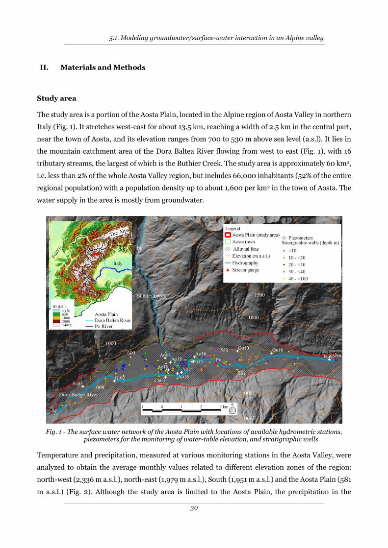
The study area is a portion of the Aosta Plain, located in the Alpine region of Aosta Valley in northern
Italy (Fig. 1). It stretches west-east for about 13.5 km, reaching a width of 2.5 km in the central part,
near the town of Aosta, and its elevation ranges from 700 to 530 m above sea level (a.s.l). It lies in
the mountain catchment area of the Dora Baltea River flowing from west to east (Fig. 1), with 16
tributary streams, the largest of which is the Buthier Creek. The study area is approximately 60 km2,
i.e. less than 2% of the whole Aosta Valley region, but includes 66,000 inhabitants (52% of the entire
regional population) with a population density up to about 1,600 per km2 in the town of Aosta. The
water supply in the area is mostly from groundwater.
Fig. 1 - The surface water network of the Aosta Plain with locations of available hydrometric stations, piezometers for the monitoring of water-table elevation, and stratigraphic wells.
Temperature and precipitation, measured at various monitoring stations in the Aosta Valley, were
analyzed to obtain the average monthly values related to different elevation zones of the region:
north-west (2,336 m a.s.l.), north-east (1,979 m a.s.l.), South (1,951 m a.s.l.) and the Aosta Plain (581
m a.s.l.) (Fig. 2). Although the study area is limited to the Aosta Plain, the precipitation in the

5.1. Modeling groundwater/surface-water interaction in an Alpine valley
31
surrounding catchment areas is also of interest because it falls mostly on impermeable upland
surface and then circulates to the plain as infiltration through alluvial debris and fans at the edge of
the valley or as spring flow. The measurements reflect climatic conditions at different elevations; the
maximum temperatures are measured in the Aosta Plain (annual average: 12.8°C), the minimum
ones in the west area (annual average: 1.7°C). The minimum monthly temperature is in January or
February, the maximum in August.
Fig. 2 - Average monthly temperature (C°) and precipitation in different sectors of the Aosta Valley Region. Number in parentheses is the topographic elevation (m a.s.l.) of the station
The maximum precipitation is generally recorded in April, although in the north-west watershed the
wet period extends from April to June. The minimum precipitation is usually in October in the South
watershed, in January in the north-east and north-west watersheds and in August in the Aosta Plain.
Except for the plain area, the precipitation is in the form of snow from November until March, and
the snow melt occurs from March until June.
Conceptual model
Hydrogeological system
The Aosta Plain is underlain by a series of fluvioglacial, lacustrine, alluvial and fan sediments,
Quaternary in age, which in turn lay on a deep crystalline basement eroded by the Balteo Glacier.
The aquifer is bounded to the north and south by the crystalline bedrock of the Alps (PIAHVA 1992).
In this sedimentary basin, a silty-sandy deposit, never completely penetrated by wells, is located at
the depth of about 50-90 m (decreasing from west to east) from the land surface and its thickness is
estimated to be over 40 m (Pollicini 1994; Triganon et al. 2003; Bonomi et al. 2013, 2015; Rotiroti
et al. 2015). This deposit of lacustrine origin is considered to act as a low-permeability basement
boundary for the overlying aquifer used for water supply. Furthermore, two recent Electric
Resistivity Tomography surveys (ERT) conducted in the towns of Aosta and Pollein during 2013

5.1. Modeling groundwater/surface-water interaction in an Alpine valley
32
(unpublished data provided by the Regional Environmental Protection Agency of Aosta Valley
(ARPA VdA)) revealed the presence of a deeper sandy-gravel aquifer (of likely glacial origin), not yet
exploited, below the lacustrine aquitard. Moreover, the ERT showed that the lacustrine aquitard has
some discontinuities (coarse deposits that act as higher permeability windows) that allow the deeper
glacial aquifer and the overlaying exploited aquifer to be interconnected.
The exploited shallow aquifer, consisting mainly of heterogeneous alluvial deposits, ranges in
thickness from 85 to 90 m in the western part to 50 m in the eastern part where the aquifer is divided
into an unconfined (about 20 m thick) and a semi-confined portion (between 25 and 12 m) by a silty
layer (Pollicini, 1994; Nicoud et al. 1999; Triganon et al. 2003).
Available hydrological and hydraulic head data
The available discharge data of the stream network between 2008-2014 were provided from the
institutional monitoring network of ARPA VdA. The streamflow data were recorded by four
hydrometric stations: Aymavilles (Ay - 618 m a.s.l.), Pollein (Po - 545 m a.s.l.), Nus (Nu - 534 m a.s.l.)
and Roisan (Bu - 742 m a.s.l.). The first three are related to the Dora Baltea River whereas the Roisan
station is related to the Buthier Creek (Fig. 1). Generally, the Dora Baltea River is characterized by
two yearly streamflow peaks respectively in June and November (Fig. 3). The first one is greater than
the second and represents the snowmelt and high precipitation period of the year, the second arises
only from the autumnal rainfall peak. With regard to 2009, in January the average streamflow at
Aymavilles (3.77 m3/s) was higher than the one at Pollein (2.51 m3/s) which was lower than at Nus
(3.06 m3/s). In June, the peak recorded at Pollein (129.73 m3/s) hydrometric station was higher than
both those at Aymavilles (109.15 m3/s) and at Nus (100.80 m3/s). As for the Butheir Creek, it had
the same yearly streamflow features of the Dora Baltea, though its discharge has always been much
lower than the previous one. For the surface water, the low flow period is usually in winter when the
temperatures are low and the precipitation is in the form of snow.
The hydraulic-heads trend analysis was carried out in order to better understand the behavior of the
aquifer. Hydraulic head data from the institutional monitoring network of ARPA VdA (Fig. 4) were
available from 2000 to 2012. Special attention was given to heads data measured within the
modelled area between 2009-2010 (selected period for the groundwater flow model). The hydraulic
head (Fig. 4) decreases from about 582 m a.s.l. (Sa03 – upstream area) to 522 m a.s.l. (Nu05 –
downstream area), suggesting a principal flow direction from west to east. Hydraulic head data show
a seasonal oscillation between the yearly maximum value in summer and the minimum value in
March-April. In particular, for the upstream area (Sa03) the oscillation is about 6-7 m and decreases
by up to 1 m while moving to the downstream area (Qu16). This sharp reduction is related to a likely

5.1. Modeling groundwater/surface-water interaction in an Alpine valley
33
draining behavior of the Dora Baltea River on the groundwater which seems to decrease starting
from Pollein hydrometric station toward the downstream area (Bonomi et al. 2015).
Fig. 3 - Average monthly streamflow (m3/s) of the Dora Baltea River (Ay, Po, Nu) and Buthier
Creek (Bu)
Fig. 4 - Water table elevation (m a.s.l.) measured in monitoring piezometers (see Fig. 1 for locations) and in
the Dora Baltea River (Po station) between 2000 and 2012 in the Aosta Plain
Groundwater flow
The water table, built using Ordinary Kriging interpolation of monthly hydraulic heads from
piezometers (monitored from ARPA VdA) and from the Po hydrometric station, is represented by
the piezometric map in Fig. 5 (January 2009).

5.1. Modeling groundwater/surface-water interaction in an Alpine valley
34
Fig. 5 - Groundwater head (January 2009) with a contour every 2 m, used as the initial condition for the
steady-state model. (modified after Bonomi et al. 2013)
As a consequence of the valley shape, the aquifer structure, and the relationships with surface water,
the piezometric heads vary from 600 to 526 m a.s.l. from west to east along the valley. The hydraulic
gradient decreases downstream: it is 1% in the western, 0.5-0.6% in the middle and 0.3-0.4% in the
eastern sector of the area.
As for the relationship between surface water and groundwater, the Dora Baltea River is losing
upstream of the Po hydrometric station (PIAHVA 1996; Triganon et al. 2003), but downstream of
the Po hydrometric station it becomes gaining with hydraulic connection (PIAHVA 1996; Triganon
et al. 2003; Bonomi et al. 2013, 2015).
The water depth decreases longitudinally from west to east and transversely from the valley slopes
to the Dora Baltea River, ranging from a maximum of around 20 m and 25 m respectively in the
western sector and in the alluvial fan of the Buthier, to a minimum of 10 m and 4 m respectively in
eastern sector, near the Dora Baltea River. This distribution restates the relationship between
groundwater and the Dora Baltea River which is losing in the western sector while it is gaining in the
eastern sector, in particular from the Po hydrometric station.
With respect to the temporal groundwater oscillations, the difference between the hydraulic head of
July and January 2009 shows that in the western area the combined effect of the narrow valley,
snowmelt and probable recharge from the Dora Baltea River causes water-level oscillations up to 6-
8 meters, while towards the widening of the valley, lower oscillations occur. Finally, in the eastern
part, the river drainage reduces groundwater head fluctuations to several meters.
Well pumping
The Aosta Plain aquifer is subjected to intense groundwater exploitation serving both drinking and
industrial supplies. Local industries are served by 19 wells located in the central and in the eastern
part of the Aosta Plain whereas the drinking water supply comprises 8 wells located in the western
part of the plain (Fig. 6a). Therefore, the total number of operating wells in the area is 27. Other wells

5.1. Modeling groundwater/surface-water interaction in an Alpine valley
35
for domestic supply exist in the study area, however, their smaller discharges are negligible for the
purposes of the present work.
Data on groundwater abstraction from these 27 wells were provided by ARPA VdA. These data
concern the monthly average well discharge (m3/hour) and the well working time (hours) for the
period 2009-2010. The total volume of groundwater pumped was 19,656,447 m3 in 2009 (82.87%
for industrial and 17.13% for drinking uses) and 2,2024,240 m3 in 2010 (81.35% for industrial and
18.65% for drinking uses). From January to August 2009 the total well discharge decreases from
63,000 to 44,000 m3/d. Between September and December 2009 a peak was recorded in October
(i.e. 69,000 m3/d) due to industrial needs. Concerning the 2010, the well discharge gradually rose
from January to July, then it fell in August representing the annual minimum (49,000 m3/d). From
September to December 2010, the discharge was quite stable around 60,000 m3/d.
Numerical model
Previous models
Although the Aosta Plain aquifer was already modelled by three previous works (Triganon et al.
2003; Bonomi et al. 2013, 2015), some key aspects concerning groundwater/surface-water
interactions remained unclear and required the development of a new improved model. A brief
description of these earlier models (and their limitations) is given in the following.
The first model presented by Triganon et al. (2003) took into account the shallower part (up to 90
m) of the Quaternary sediments subdividing it into two layers. Only the Dora Baltea River was
simulated using the RIV package, hence without considering its discharge. The hydraulic
conductivity was discretized in four isotropic zones of piecewise constancy with the same distribution
between layers. This steady state model provided a preliminary analysis on the effects of the surface
water level on both the water table elevation and the water exchanged between the main river and
groundwater. The coarse refinement of the grid and the hydraulic conductivity coupled to the use of
the RIV package led to rough estimates for results, in particular, concerning the amount of
exchanged water between the river and aquifer.
Bonomi et al. (2013) presented a steady state model, which considered the whole hydrographic
network of the Aosta Plain simulated by the SFR2 Package and MODFLOW2000. That work focused
on the definition of a preliminary conceptual model of the aquifer in order to improve the general
knowledge of the system. However, the use of a steady state condition prevented the understanding
of the temporal variations on groundwater/surface-water interactions.
Bonomi et al. 2015 improved their previous work implementing a transient model based on monthly
recharge values with the aim of simulating the seasonal oscillation of the water table, however no
evaluations of the water budget and exchanged fluxes were done.

5.1. Modeling groundwater/surface-water interaction in an Alpine valley
36
In order to overcome the limitations of the above-mentioned previous models, the present work
implements the following new aspects: (1) a new reconstruction of the system geometry that
incorporates the deeper glacial aquifer which is likely interconnected with the shallower units as
evidenced by new available data (i.e. ERT surveys and new well logs, see section 2.2.1); (2) an
improved three-dimensional reconstruction of the hydraulic conductivity distribution (see the
Electronic Supplementary Material - ESM for details) in order to include the new available well logs;
(3) an automatic calibration, using PEST, for estimation of model parameters.
Nevertheless, the detailed calculation of monthly recharge inputs made by Bonomi et al. (2015) is
retained in the present work. These recharge values were calculated as the water average surplus
obtained by the Thornthwaite-Mather’s hydrological balance model starting from the average
monthly precipitation and temperature data (available only for 2009 and 2010 and calculated for
the different regional watersheds; Fig. 2).
Hydraulic conductivity reconstruction
In order to reconstruct the spatial distribution of hydraulic conductivity, the TANGRAM© database
was used (Tangram, 2016; Bonomi et al. 2014). This database is meant to manage administrative,
borehole construction, stratigraphic and piezometric information. TANGRAM© has an internal
coding system that allows the standardization of stratigraphic information and the extraction of
stratigraphic data in terms of hydraulic conductivity (k), according to depth, measured at the meter
scale in the present work. The hydraulic conductivity values of 176 stratigraphic logs were extracted
from TANGRAM© in order to obtain a XYZk point dataset, where X and Y are coordinates in the
UTM system, Z is the elevation (m a.s.l.) and kis the hydraulic conductivity value (in terms of ln(k)).
The values of hydraulic parameters are defined in relation to textural percentages (Bonomi et al.
2002; Bonomi et al. 2009), by means of a conductivity data conversion table integrated into the
TANGRAM© database. The distribution of hydraulic conductivity was assumed to be lognormal
(Martin and Frind 1998) and a well-known method (Dagan and Lessoff 2007; Dagan 2012) for
calculating the weighted standard mean (Sanchez-Vila et al. 1995) of hydraulic conductivity values
attributed to the individual lithologies was followed (ranging from 436 m/d for gravel to 0.864 m/d
for silty-clay; for more details on the interpolation see the ESM).
For this study, the hydraulic conductivity values assigned to the conversion table in TANGRAM©
were previously calibrated by trial and error on the basis of nine pumping tests reported in literature
(Pollicini 1994; De Luca et. al 2004). The calibration was focused on the minimization of the
difference between the ln(k) value calculated by TANGRAM© and the ln(k) value from the literature.
The coded lithologs were imported into a 3D grid and interpolated by geostatistical approach in
GOCAD®. The GOCAD® code (Geological Object Computer Aided Design, Paradigm 2008) was used

5.1. Modeling groundwater/surface-water interaction in an Alpine valley
37
to build the computational grid, then apply the geostatistic technique of Ordinary Kriging, based on
the assumption of stationary spatial conditions with respect to the statistical distribution of the
subsurface stratigraphic data. For more details on the interpolation see the Interpolation Grid
section of the ESM.
Model design
This work is the evolution of specific existing models (Bonomi et al. 2013, 2015). Indeed, data about
hydrogeological balance (e.g. recharge, pumping rate, river parameters) derive from these previous
works. They have been integrated with new information allowing researchers to improve the
knowledge of the investigated aquifer.
The model grid has 3,183,300 cells divided in 243 rows and 655 columns with a uniform cell spacing
of 20x20 m, covering an area of ~60 km2 (active cell ~25 km2). The vertical discretization of the grid
reflects the stratigraphic grid used for the interpolation of the hydrogeological parameters. It consists
in twenty layers: eighteen of them have a constant thickness, whereas two (second and third layers)
are variable (Min 0.8 m; 25th percentile 5.6 m; median 10.4 m; 75th percentile 20.2 m; Max 72.8
m). The first sixteen layers were used to model the exploited aquifer, whereas the last four layers (90
m thick) were used to consider the silty layer (lacustrine aquitard of the main shallow aquifer; see
section 2.2.1) and the underlying coarse (gravelly-sand) deposits recorded by ERT. The refinement
of the vertical spacing helps to capture hydrogeologic trends and allows the model to closely match
the intervals over which pumping wells are screened, thereby increasing the accuracy of the model
in simulating withdrawals. Furthermore, the low thickness of the upper layers has allowed an
accurate positioning of the riverbed, improving the simulation of the rivers and groundwater
interaction.
The complex three-dimensional reconstruction of hydraulic conductivity (Fig. S1 of the ESM) was
subsequently discretized in ten zones of piecewise constancy by means of the analysis of the
frequency distribution of the obtained hydraulic conductivity. As for the last four layers, two
additional zones were defined: in the central part was assigned a low value (0.0864 m/d) in order to
reproduce the silty-clay lacustrine layer, whereas at the edge a high value (69.12 m/d), typical of the
sandy deposit, was assigned. The groundwater flow equation of a transient model is complicated by
another term representing the aquifer storage capability (i.e. specific storage (Ss) and a specific yield
(Sy)). As for the storage, the discretization in zones was obtained from the hydraulic conductivity
distribution, whereas the values were selected from literature. In particular, the assigned values on
each zone varied between 0.05 and 0.28 for Sy, and between 5x10⁻⁶ and 1.5x10⁻⁴ for Ss (Domenico
and Mifflin 1965). The obtained conductivity/porosity zones and their values became the basis for
the flow model.

5.1. Modeling groundwater/surface-water interaction in an Alpine valley
38
The used code was MODFLOW 2005 (Harbaugh 2005), visualized through the GroundwaterVistas6
interface (Rumbaugh and Rumbaugh 2004).
The model was solved both in steady-state and transient condition with GMG package and
considering the rewetting capability. The steady-state configuration was referred to January 2009 in
order to reproduce an average condition of the aquifer between 2000 and 2012 (Fig. 4). The transient
analysis was limited to a two-year period (2009-2010) using 24 stress periods (one per month). This
approach allowed both evaluation of the non-steady-state model response to variable stresses
(Taviani and Henriksen 2015) and evaluation of how the change of the water balance during seasons
takes into account the storage component. The choice of the selected simulated period was mainly
related to the availability of measured data on well abstractions (see section 2.24.). This is a key
aspect since the main goal of this work is to understand the effects of well pumping on the
relationship between groundwater and surface water. The use of measured discharges rather than a
speculative estimation of their values is preferred since it decreases the uncertainty and increases
the accuracy of model results.
The streamflow data of the Dora Baltea River and Buthier Creek in addition to the piezometric and
precipitation data referred to 2009-2010 were used both in the steady state model (January 2009)
and in the transient one (2009-2010).
In order to evaluate the impact of wells on both rivers and groundwater, simulations with different
configurations of the pumping were conducted (Feinstein et al. 2010; Barlow and Leake 2012). The
transient solution with 27 active wells (baseline scenario) was compared with two new scenarios.
Each new scenario differs from the baseline scenario in the discharge value of only one well: scenario
A, which aims to evaluate the effects of well pumping in the upstream area where the Dora Baltea
River is losing, considers an increase of 1,000 m3/d for the discharge of the well W_US (see location
in Fig. 9); scenario B, concerning the effects of pumping in the downstream area where the Dora
Baltea River is draining, considers an increase of 1,000 m3/d for the discharge of the well W_DS (see
location in Fig. 9). Results of the different scenarios where compared through the analysis of the
MODFLOW mass balance output file (i.e. *.lst file).
Boundary hydraulic conditions
The boundary conditions were defined on the basis of the hydrogeological configuration of the Aosta
Plain and the piezometric trend of the period 2009-2010. The conditions imposed are: 1) No Flow,
Neumann-type boundary conditions, at the northern and southern edges of the plain, at the
boundary between fan deposits and the slope. In depth, the limit to no-flow defines the geological
shape of the valley, cut in the western part and progressively widening towards the east (Bonomi et
al. 2014). 2) General Head Boundary (Cauchy-type boundary conditions), at the western and eastern
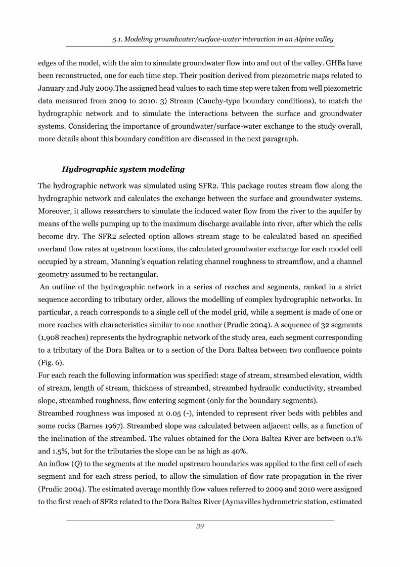
5.1. Modeling groundwater/surface-water interaction in an Alpine valley
39
edges of the model, with the aim to simulate groundwater flow into and out of the valley. GHBs have
been reconstructed, one for each time step. Their position derived from piezometric maps related to
January and July 2009.The assigned head values to each time step were taken from well piezometric
data measured from 2009 to 2010. 3) Stream (Cauchy-type boundary conditions), to match the
hydrographic network and to simulate the interactions between the surface and groundwater
systems. Considering the importance of groundwater/surface-water exchange to the study overall,
more details about this boundary condition are discussed in the next paragraph.
Hydrographic system modeling
The hydrographic network was simulated using SFR2. This package routes stream flow along the
hydrographic network and calculates the exchange between the surface and groundwater systems.
Moreover, it allows researchers to simulate the induced water flow from the river to the aquifer by
means of the wells pumping up to the maximum discharge available into river, after which the cells
become dry. The SFR2 selected option allows stream stage to be calculated based on specified
overland flow rates at upstream locations, the calculated groundwater exchange for each model cell
occupied by a stream, Manning's equation relating channel roughness to streamflow, and a channel
geometry assumed to be rectangular.
An outline of the hydrographic network in a series of reaches and segments, ranked in a strict
sequence according to tributary order, allows the modelling of complex hydrographic networks. In
particular, a reach corresponds to a single cell of the model grid, while a segment is made of one or
more reaches with characteristics similar to one another (Prudic 2004). A sequence of 32 segments
(1,908 reaches) represents the hydrographic network of the study area, each segment corresponding
to a tributary of the Dora Baltea or to a section of the Dora Baltea between two confluence points
(Fig. 6).
For each reach the following information was specified: stage of stream, streambed elevation, width
of stream, length of stream, thickness of streambed, streambed hydraulic conductivity, streambed
slope, streambed roughness, flow entering segment (only for the boundary segments).
Streambed roughness was imposed at 0.05 (-), intended to represent river beds with pebbles and
some rocks (Barnes 1967). Streambed slope was calculated between adjacent cells, as a function of
the inclination of the streambed. The values obtained for the Dora Baltea River are between 0.1%
and 1.5%, but for the tributaries the slope can be as high as 40%.
An inflow (Q) to the segments at the model upstream boundaries was applied to the first cell of each
segment and for each stress period, to allow the simulation of flow rate propagation in the river
(Prudic 2004). The estimated average monthly flow values referred to 2009 and 2010 were assigned
to the first reach of SFR2 related to the Dora Baltea River (Aymavilles hydrometric station, estimated

5.1. Modeling groundwater/surface-water interaction in an Alpine valley
40
net of diversion) and the Buthier Creek, whereas for the remaining streams it was estimated on the
basis of information gathered and occasional ARPA VdA measurements.
Model recharge and discharge
As remarked by Bonomi et al. (2015), the recharge of the studied aquifer is closely related to the
snowmelt (occurring from April to July) which, in turn, is related to both the quantity of snow
occurring in winter and the increase of the temperature during following seasons. The recharge was
imposed through 4 zones and using monthly time steps (Bonomi et al 2015). The minimum imposed
value was 0.099 mm per month in the central part of the plain in January 2010, whereas the
maximum value was 2292.14 mm per month per day in the southern-west of the plain in May 2009.
Another important stress and element of the hydrologic budget is well withdrawal. Measured
monthly well withdrawals were assigned to the 27 operating wells (see section 2.2.4) depending on
their own flow rate, ranging between 0.26 and 18,000 m³/d. The screen lengths and depths were
inserted for each well, and they are distributed between 20 m and 80 m in depth.
Calibration and Target
Both hydraulic head target and flux target were used to calibrate the model. The head targets were
compiled from the piezometric monitoring network of ARPA VdA (Fig. 1) on a monthly basis or
quarterly data. It was considered inappropriate to define an allowable error in the head target
comparison values (Sonnenborg et al. 2003) both because the data are the actual monthly
measurements (not derived from the mean of data referred to longer periods) and because it is
considered reliable (ARPA VdA monitoring). Local errors might still be related to piezometric
measurements influenced by the pumping of the surrounding wells. The number of hydraulic head
observations was 25 for the steady-state condition and 348 for transient simulation heterogeneously
distributed among 37 head target.
The flux target (ARPA VdA monitoring) is located in the central area of the model (Po hydrometric
station - Fig. 1). The flux target reported 24 values defined as the monthly average of the daily
streamflow recorded by Po hydrometric station between 2009 and 2010. All targets are shown in
Fig. S3 of the ESM.
The model calibration was done on the steady state model using PEST (Doherty 2008, Doherty and
Hunt 2010). A preliminary sensitivity analysis on hydraulic parameters (kx=kv, kz=kx/10) and SFR2
conductance was performed on the steady-state model. All of those most sensitive parameters (>1%)
were selected for the calibration process (Hill 1998). A reasonable upper and lower bound was
applied to the initial value of each selected parameter (±50% of the starting value for k and 0.0001
to 5 (m/d) for the stream bed conductivity). The obtained calibrated model was employed as a
starting condition for the transient model. To improve the performance of the transient model and

5.1. Modeling groundwater/surface-water interaction in an Alpine valley
41
to better reproduces the strong oscillation of the water table, a second calibration was carried out by
PEST. A new sensitivity analysis on storage values (Ss and Sy) and hydraulic conductivity (kx=ky)
was done (Fig. S4 of the ESM). Parameters with sensitivity more than 1% of the greatest value of the
composite sensitivity were calibrated applying reasonable upper and lower bounds (Table 1).
Table 1 – Applied bounds and final values of the selected parameters (k - m/d, ss - 1/m) by sensitivity
analysis
initial lower upper final
kx_2 gravel 571 143 1000 517.943
kx_3 sandy gravel 127 32 222 197.34
kx_4 sand (semi_conf Po) 100 25 175 162.65
kx_7 sandy gravel (fan) 164 41 289 253.25
kx_11 sand (unexp_acq) 69 17 121 101.11
kx_12 silty clay (deep aquitard) 42 11 74 37.04
Ss_1 silty clay (deep aquitard) 5x10⁻⁴ 2.5x10⁻⁴ 7.5x10⁻⁴ 6.03x10⁻⁴
Sy_3 sandy gravel 0.2 0.01 0.28 0.17

5.1. Modeling groundwater/surface-water interaction in an Alpine valley
42
III. Results and Discussion
Steady state simulation (January 2009)
The choice of January is connected to the flow rate of the surface system, which is representative of
the low-flow period (Feinstein et al. 2010); in fact as shown before, this is the month when the water
table is lowest and the runoff from stormflow is largely absent. Furthermore, January 2009
represents an average condition of the aquifer during the last decade.
Fig. S5 of the ESM shows the distribution of the calibrated value of the hydraulic conductivity within
layer 4. The values of this parameter are in agreement with previous studies on the Aosta Plain
(Triganon et al. 2003; Bonomi et al. 2013, 2015; Stefania et al. 2015) ranging between 0.0864 m/d
to 572 m/d.
The Dora Baltea River conductance was calibrated starting from a hydraulic conductivity of 1 m/d.
As a result of the calibration, it changes among 0.15 m/d in the western part to 0.01 m/d in the
central part and it increases to 4 m/d in the eastern part (Hatch et al. 2010) (Fig. 6 a).
The simulated head, which takes into account the wells pumping and the exchange between rivers
and groundwater, produced the piezometric configuration shown in Fig. S3 of the ESM. It represents,
with spacing of 1 m, a variation of head from 580 m a.s.l. in the west to 526 m a.s.l. in the east, and
a flow direction west-east. It closely reproduces the variations of the gradient, which increases from
the west towards the Aosta Plain, decreases near the areas with high hydraulic conductivity around
the fan of the Buthier and increases again towards the downstream sector.
The solution has the following statistics: the residuals ranged from -0.96 m to +0.94 m, with a
Residual Mean of -0.02 m, Absolut Residual Mean of 0.40 m, and a Scaled Root Mean Square value
of 1%, and the sum of square residuals (the square root of the average of the squared error, Anderson
and Woessner 1992) was 5.63.
The simulated flux at the Po hydrometric station (2.76 m3/s) appears in good agreement with the
observed one (2.55 m3/s), considering the observed Dora Baltea River discharge and all of the factors
that cause it, among which: 1) the diversion near Aymavilles hydrometric station, 2) tributaries
discharge contribution, 3) exchange between surface water and groundwater.
With regard to the mass balance (which has an error less than 0.001%), approximately 21,521 m³/d
are conveyed into the model due to the recharge contribution, and about 62,849 m³/d exit due to 27
wells. In the present configuration, the surface water system recharges the aquifer at a rate of 132,534
m³/d (IN from stream to aquifer), and drains the aquifer at a rate of about 90,130 m³/d after the Po
hydrometric station (OUT to the stream).
In the central area of the Aosta Plain, around the fan of the Buthier, the simulated head shows values
higher and lower than the observations (Fig. S3 of the ESM). These discrepancies may be associated

5.1. Modeling groundwater/surface-water interaction in an Alpine valley
43
to different aspects: a) an in-depth analysis is necessary for a better description of heterogeneities
distribution which
Fig. 6 – (a) Segment numbers and streambed hydraulic conductivity values (m/d) of the Dora Baltea River and its tributaries, and locations of pumping wells. (b) The difference in drawdown between pumping and
no pumping scenarios (m). (c) Average monthly exchange between the Dora Baltea River and the surrounding aquifer for each segment (m3/d); blue bars represent the pumping scenario and red bars
represent the no-pumping scenario.
regulate groundwater flow on a local scale, b) the attribution of monthly average pumping rate values
in the model, whereas the real hourly flow rate might have influenced the measured water levels,
generating noise in the targets which is not reproducible by the simulation, c) the real head target
values represent monthly average levels and they may not be perfectly correlated with monthly
pumping. In the eastern part, the simulated head suffers from an overestimation. This result suggests
that as to the downstream area, probably, further geological investigations should be considered, to
correctly understand how the water leaves the modelled area through the narrowing of the valley
edges. In order to evaluate the impact of well pumping on the water table and stream depletion, a
simulation without pumping was done, then it was compared with the calibrated solution. The
simulation without pumping shows a considerable rise of the water table especially in the central

5.1. Modeling groundwater/surface-water interaction in an Alpine valley
44
part of the area where the wells’ withdrawal is bigger. In this area, beneath of the Aosta town, the
water table was pushed down more than 5 m due to well pumping (Fig. 6b). Table 2 shows the
changes induced by pumping on water balance. Overall, the pumping limits the amount of the water
gained by the Dora Baltea River (~34,400 m3/d) and increases its leakage (~16,300 m3/d). This
result highlights that surface water is an important part of the hydraulic budget of the Aosta Plain.
The groundwater/surface-water exchanges (average flux m3/d) along the Dora Baltea River are
shown graphically to emphasize their spatial variability for both pumping and no pumping scenarios
(Fig. 6). The drawdown induced by the wells’ withdrawal not only affects the shape of the water table,
in fact, it also induces changes on the surface/groundwater exchange flux with a slight increase of
the stream leakage by segment 11 and about one order of magnitude from the segment 17. Segment
18 shows the greatest variation with a sharp decrease of the water drainage (e.g. from 490 to 21 m3/d)
as a result of the groundwater depletion. Also segments 20, 22 and 24 decrease their drainage flux,
however, less than the previous one. The largest difference of water exchange recorded in segment
18 is related to the downstream moving of the transition point from losing to gaining behaviour of
Dora Baltea River. This transition point is located within segment 18 in both scenarios, however, its
movement downstream in the pumping scenario, due to water-table lowering, leads to a decrease of
the water drained by the river. In the central area (close to segment 13 and 15), the water-table
elevation never exceeds the riverbed elevation thus preventing any variation of water exchange
between the river and aquifer.
Table 2 – Water balance (m3/d) for the pumping and no-pumping scenarios.
Pumping (P) No Pumping (NP) Pumping vs No Pamping
Terms of the
water balance IN OUT IN OUT IN_P-IN_NP OUT_NP-OUT_P
General Head
Boundary 30282 31356 19579 32759 10703 1403
Recharge 21521 21524
Well
withdrawal 62849
Dora Baltea
River 82231 90130 66017 124544 16213 34414
Tributaries 50304 50185 119
Total 184337 184335 157305 157303 27035 35817

5.1. Modeling groundwater/surface-water interaction in an Alpine valley
45
The well pumping has no influence on the tributary streams (Table 2) because a) the great
unsaturated thickness (around 30 m on average and up to 96 m) beneath tributary streams prevents
any direct interaction between the tributary water and groundwater; b) the greater slope of the
riverbed up to 0.45% (Bonomi et al. 2013) increases the water flowing velocity while, on the other
hand, decreasing the possibility of its infiltration toward groundwater; c) the available discharges of
the tributary streams are about two orders of magnitude lower than the main river. Furthermore,
some of the tributary streams (i.e. segments 2-6-8-14-25-27-29) have an impermeable riverbed that
prevents any water exchanges.
Transient simulation (January 2009 - December 2010)
Models with two different sets of hydraulic parameters were compared (Fig. 7). The new set of
parameters obtained by the second analysis of sensitivity (Fig. S4 of the ESM) and subsequent
recalibration (Table 1), as defined in Section ‘Calibration and target’, better reproduces the
hydraulic head trend both upstream and downstream of Aosta town (Fig. 7). The spatial and
temporal behavior of residuals between observed and simulated values highlights that the first
solution with respect to the recalibrated solution, overestimates the hydraulic head, especially during
the low flow periods, inducing a water accumulation in the downstream area.
The analysis of sensitivity has shown that the water accumulation was dependent on both storage
and conductivity parameters. Another important aspect was that the newest calibrated values
remained consistent with those that were initially derived from the TANGRAM database (see section
2.3.2), however a slight increase of the values (except to sy_3) was observed. With regard to the
reconstruction of the streamflow of the Dora Baltea River, the modelled discharge (Fig. 7) compared
with the measured data was in good agreement, even if it has not correctly reproduced the fall in
discharge peaks. However, the modelled streamflow seems to be acceptable taking into account that
the discharge of tributaries has been estimated and the hydraulic conductivity is a challenging
parameter to be estimated (Hatch et al. 2010).
Comparing the simulated water table with the bottom elevation of the Dora Baltea River, it becomes
clear how the piezometric oscillation affects the Aosta Plain aquifer during the seasons and how it
changes their relationship along the investigated area (Fig. S6 of the ESM). Upstream of Aosta town,
the distance between the water table beneath the streambed and the stream bottom decreases
steeply, with occasionally sharp reduction dependent on streambed jumps.
Close to Aosta town, the water table falls, probably due to the wells’ withdrawal with a variable
magnitude which changes seasonally. Another important outcome is that some of the Dora Baltea
reaches located upstream of Aosta town change from losing to gaining and vice-versa. In fact,
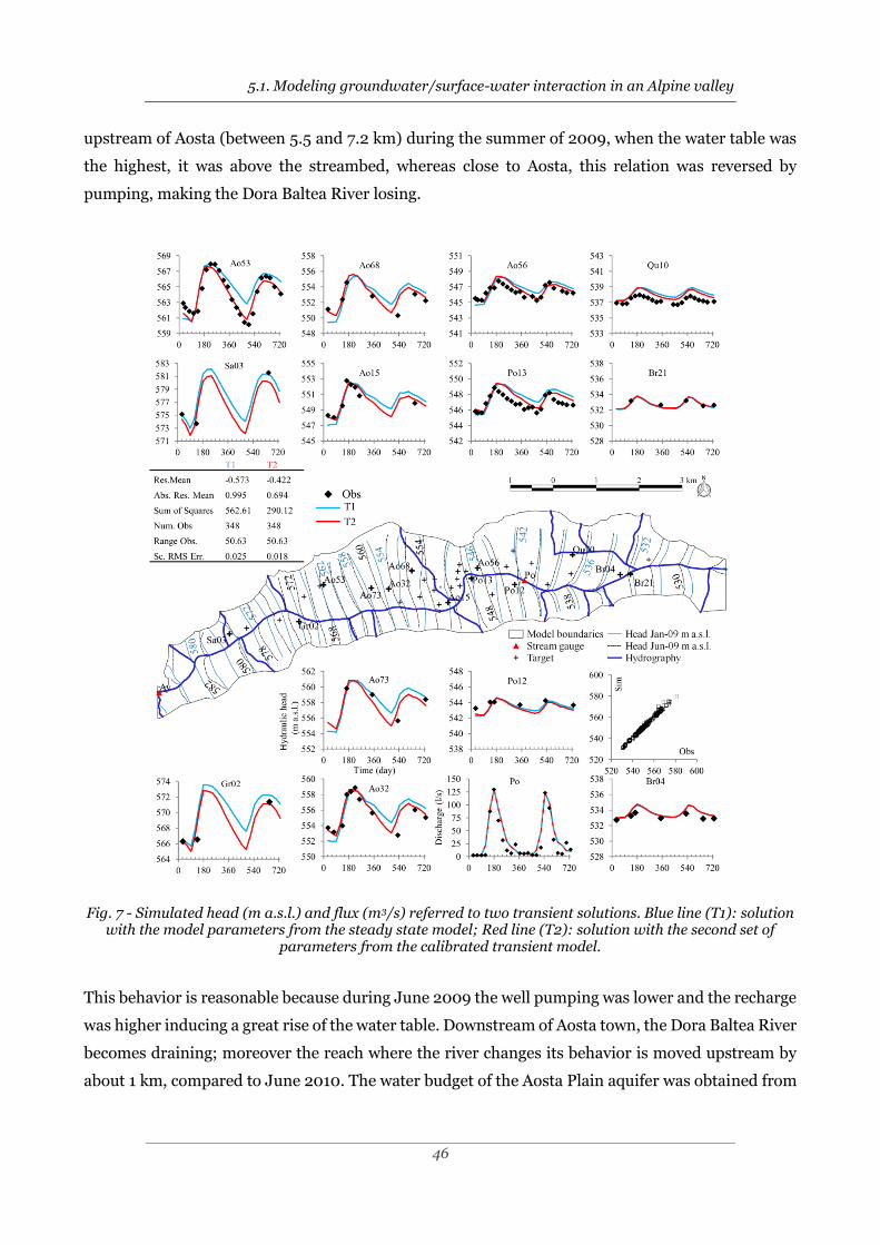
5.1. Modeling groundwater/surface-water interaction in an Alpine valley
46
upstream of Aosta (between 5.5 and 7.2 km) during the summer of 2009, when the water table was
the highest, it was above the streambed, whereas close to Aosta, this relation was reversed by
pumping, making the Dora Baltea River losing.
Fig. 7 - Simulated head (m a.s.l.) and flux (m3/s) referred to two transient solutions. Blue line (T1): solution with the model parameters from the steady state model; Red line (T2): solution with the second set of
parameters from the calibrated transient model.
This behavior is reasonable because during June 2009 the well pumping was lower and the recharge
was higher inducing a great rise of the water table. Downstream of Aosta town, the Dora Baltea River
becomes draining; moreover the reach where the river changes its behavior is moved upstream by
about 1 km, compared to June 2010. The water budget of the Aosta Plain aquifer was obtained from

5.1. Modeling groundwater/surface-water interaction in an Alpine valley
47
the transient simulation (Fig. 8): it is characterized by two peaks of inflow due to recharge during
the spring 2009-2010.
Fig. 8 - Water budget of the transient solution. Negative values (dashed line) represent water leaving the aquifer, whereas positive values (continous line) represent water entering the aquifer.
The hydrography network is both an inflow and an outflow: the latter increases when the water table
is higher (summer), confirming that the water table oscillation is reduced by the river drainage
especially in the downstream area. The greater river inflow occurs during the periods of most
infiltration, confirming that snowmelt plays a key role in the recharge of the groundwater system. As
for the storage, it appears an important element of the groundwater budget because it acts as a tank.
In fact, the aquifer is recharged during the water-available periods (SINK element) and becomes a
source of water during the low flow period, typically in winter. In October 2009 there is the highest
well withdrawal (about 69,000 m3/d) which induced the most important outlet from the storage.
These results have highlighted that the Aosta Plain aquifer storage capability is a key aspect of the
groundwater system which together with recharge and surface water seepage/drainage, contributes
to the complex dynamics that occur on the studied aquifer, allowing fluctuations of the water table
more than 5 m in amplitude.
Impact of wells on the groundwater and river budget
The first important feature which emerges and confirms the goodness of the obtained groundwater
model is that it is able to give back the imposed increase on the well discharge without producing
mass balance errors. The obtained results highlight two different behaviors of the aquifer: in
downstream area (i.e. Scenario B) the

5.1. Modeling groundwater/surface-water interaction in an Alpine valley
48
Fig. 9 - Well-pumping impact on the groundwater and surface water balance. W_US: well located in the upstream area; W_DS: well located in the downstream area. The legend shows the formulas used for the calculation of the flux variations induced by well pumping (i.e. W_US and W_DS), between the reference
solution (baseline scenario) and (a) scenario A and (b) scenario B.
water to the well comes mainly from the river, whereas for the upstream area (i.e. Scenario A)
different elements of the water budget actively contribute to the well discharge. In particular, as for
the well in the downstream area (W_DS in Fig. 9b), about 80% of the extracted water, for each
considered period, would have reached the river (stream diverted) adding itself to the baseflow
component of the river flow, but it is instead pumped out by the well. The fact that the impact of
W_DS well on the budget is constant over time strengthens the hypothesis that, in the downstream
area, the river is hydraulically connected with the aquifer and it acts on the water table, regulating
its seasonal oscillations and the exchanged fluxes. As for the well in the upstream area (W_US in
well (Fig. 9a), the pumped water comes from different budget items (i.e. aquifer storage, river,
upstream groundwater inflow simulated by the GHB). In particular, the contributions of the storage
and the river (e.g. stream induced = water induced through the riverbed) change over time as a
function of the hydraulic condition of the aquifer and river. In fact, when the water table is the lowest
(e.g. February 2009) then the well pumping is not able to abstract water from the river because the
flow through the unsaturated zone is likely low, consequently the water is mainly produced from the
storage (Sanz et al. 2011). Instead, when the water table is higher (e.g. June 2009), then the well
water is mainly from the river (stream induced). For the two other periods referred to W_US, the
well impact on the water balance is similar between the lower and higher period because the water
table elevation changes less than the previous periods (Fig. S6 of the ESM). Nevertheless, for the
higher period (i.e. June 2010), the amount of induced water from the river is more than the amount

5.1. Modeling groundwater/surface-water interaction in an Alpine valley
49
induced during the lower period (i.e. January 2010), confirming that the water table oscillation plays
a key role in the water exchanges between the groundwater and surface water.
IV. Conclusion
This work dealt with the modelling of an Alpine valley aquifer in the Aosta Valley Region, assessing
the water exchanges occurring between the main regional river (i.e. Dora Baltea River) and the
underlying shallow aquifer. After having defined the conceptual model of the system and
reconstructed the distribution of the hydraulic parameters, a steady state model was calibrated on
the low flow period and an evaluation of the pumping from the whole well system was performed.
The steady state model was used to initialize a two-year transient model by which both the water
table oscillation during the seasons and the impact of the pumping on the groundwater/surface water
budget were evaluated. This work has improved the understanding of the Aosta Plain aquifer, in
particular:
I. the reconstruction of the hydraulic parameters shows an aquifer mainly characterized by a
gravelly and sandy deposit with a local silty-clay layer especially in the downstream area;
II. the main recharge of the aquifer derives from the slope region, and only secondarily from
infiltration on the plain. The obtained recharge rate is typically highest during the summer
as a result of high precipitation and snow melt. This explains the wide range of water table
oscillation which affects the studied aquifer;
III. the calibration phase, using head and flux targets, has demonstrated the importance of the
three-dimensional reconstruction of the system heterogeneity for the model response;
moreover the calibration analysis suggested that the modification of the streambed
conductivity and also a few other hydraulic parameters, especially Sy and Ss, have turned out
to be influential parameters to achieving a good fit on targets;
IV. the model highlighted that from west to east of the valley, the Dora Baltea River changes its
relation with the aquifer, acting as a source of water in the upstream area and as a sink in the
downstream area. The analysis on the whole well pumping system determined that it limits
the amount of the water-gaining by the main river (~34,400 m3/d) and increases its leakage
(~16,300 m3/d). The seasonal changes in the water table elevation play a key role in the
relationship between the river and the underlying aquifer. Furthermore, it is evident that the
rising of the water table, typically in summer, is a consequence of the recharge (in the form
of infiltration) which during its higher discharge months is linked to snowmelt. Another key
aspect is related to the storage parameters, that allow either to retain or to release the water
as a function of the stress (natural and anthropogenic) to which the aquifer is subject;

5.1. Modeling groundwater/surface-water interaction in an Alpine valley
50
V. in the downstream area, the water table is always above the riverbed surface, meaning that
the river is a sink for the aquifer. In this area, about 80% of the water pumped by the selected
well comes from the base flow component of the river discharge, during the whole simulated
period. In the upstream area, the water table is always beneath the riverbed; however, during
only one of the two simulated high flow periods, along a river segment (1.5 km length), the
water table overcomes the riverbed by 0.5 m. In this area the contribution of the well
pumping components of the water budget changes as a function of the hydraulic conditions
of the aquifer, however the stream depletion is always less than the depletion with respect
the downstream area.
In conclusion, the upstream area is a better location for a new well to be drilled, because pumping
will affect the river discharge less than in the downstream area.
The present work showed that the use of SFR2 Package may be extended to a particular
hydrogeological context (i.e. Alpine valley aquifers) where complex relationships between the river
and groundwater could change over space and time due to natural factors (e.g. recharge) and/or
human activities (e.g. well pumping). The methodology presented here allows researchers to evaluate
the impact of the well pumping on the whole system in terms of both the water table lowering and
depletion of exchanged water between the river and aquifer. Furthermore, it is able to assess the
origin of the water pumped by wells.
This work can provide to decision-makers and stakeholders a useful tool to understand, manage and
quantify the aquifer and the streamflow depletion, not as separate entities, but by considering them
as an integrated system. Furthermore, it could be used to simulate the transport of dissolved
pollutions, evaluating their impact both on groundwater and surface water (Bonomi et al. 2015;
Stefania et al. 2015; Rotiroti et al. 2015).
Acknowledgments
Funding was provided through the scientific collaboration number 2-18-2009100-3 with the
Regional Environmental Protection Agency - Aosta Valley Region. The authors are grateful to Sara
Taviani, University of Milano-Bicocca, for the support received. The Gocad Research Group and
Paradigm Geophysical are acknowledged for welcoming the University of Milano-Bicocca into the
Gocad Consortium (http://www.ring-team.org/home).

5.1. Modeling groundwater/surface-water interaction in an Alpine valley
51
References
Alley WM (2007) Another water budget myth: The significance of recoverable ground water in
storage. Ground Water 45:251. doi: 10.1111/j.1745-6584.2006.00274.x
Alley WM, Reilly TE, Franke OL (1999) Sustainability of Ground-Water Resources, U.S. Geological
Survey Circular 1186. US Geol Surv Circ 1186 79.
Anderson MP, Woessner WW, (1992) Applied Groundwater Modeling: Simulation of Flow and
Advective Transport. Aca- demic Press, 381Armstrong M (1998) Basic Linear Geostatistics.
Springer Verlag, Berlin, 153 pp
Barlow PM, Leake SA (2012) Streamflow depletion by wells--Understanding and managing the
effects of groundwater pumping on streamflow (No. 1376, pp. i-84). US Geological Survey.
Barnes HH (1967) Roughness characteristics of natural channels. No. 1849. US Govt. Print. Off.,,
1967.
Bonomi, T, Cavallin A, Stelluti G, Guerra G (2002) 3-D subsoil parameterisation in a plan region of
north Italy. Memorie della Società Geologica Italiana, 57, 543-550.
Bonomi T (2009) Database development and 3D modeling of textural variations in heterogeneous,
unconsolidated aquifer media: Application to the Milan plain. Comput Geosci 35:134–145. doi:
10.1016/j.cageo.2007.09.006
Bonomi T, Fumagalli L, Benastini V, Rotiroti M, Capodaglio P, Simonetto F (2013) Modellazione
preliminare del flusso idrico sotterraneo e delle interazioni con le acque superficiali: piana di
Aosta. (Preliminary groundwater modelling by considering the interaction with superficial
water: Aosta plain case (northern Italy)). Acq. Sott.-Ital. J. Groundwater- doi: 10. 7343/AS-017-
13-0041
Bonomi T, Fumagalli L, Rotiroti M, Bellani A, Cavallin A (2014) Banca dati idrogeologica
TANGRAM©: strumento per elaborazioni quantitative di dati per la valutazione delle acque
sotterranee (The hydrogeological well database TANGRAM©: a tool for data processing to
support groundwater assessment). Acq. Sott.-Ital. J. Groundwater- doi: 10.7343/AS-072-14-
0098
Bonomi T, Fumagalli M L, Rotiroti M, Perego R, Simonetto F, Capodaglio P (2015). Groundwater
Flow Modelling of the Aosta Plain in Northern Italy. In Engineering Geology for Society and
Territory-Volume 3 (pp. 227-230). Springer International Publishing. doi: 10.1007/978-3-319-
09054-2_46
Bonomi T, Fumagalli L, Stefania GA, Rotiroti M, Pellicioli F, Simonetto F, Capodaglio P (2015)
Groundwater contamination by Cr(VI) in the Aosta Plain (northern Italy): characterization and
preliminary modeling. Rend online della Soc Geol Ital 35:21–24. doi: 10.3301/ROL.2015.54
Dagan G (2012) Flow and transport in porous formations. Springer Science & Business Media.

5.1. Modeling groundwater/surface-water interaction in an Alpine valley
52
Dagan G, Lessoff SC (2007) Transmissivity upscaling in numerical aquifer models of steady well
flow: Unconditional statistics. Water Resour Res 43:1–12. doi: 10.1029/2006WR005235
De Luca D, Masciocco L, Motta EV, Tonussi M (2004) Studio geologico finalizzato alla definizione
delle aree di salvaguardia dei pozzi di acquedotto del comune di Aosta (A geological study aimed
at defining the well protection areas of the wells in the Aosta town.). Università degli Studi di
Torino e Comune di Aosta.
Doherty J (2008a) PEST, model independent parameter estimation: user manual, 5th edn.
Watermark, Brisbane, Australia. http://www.pesthomepage.org/Downloads.php. Accessed
October 1, 2009
Doherty J (2008b) PEST, Model independent parameter estimation: addendum to user manual, 5th
edn. Watermark, Brisbane, Australia. http://www.pesthomepage.org/Downloads.php.
Accessed October 1, 2009
Doherty J, Hunt R (2010) Approaches to highly parameterized inversion: a guide to using PEST for
groundwater-model calibration. U S Geol Surv Sci Investig Rep 2010-5169 70. doi: 2010-5211
Domenico PA, Mifflin MD (1965) Water from low-permeability sediments and land subsidence,
Water Resources Research, vol. 1, no. 4., pp. 563-576
Feinstein DT, Hunt RJ, Reeves HW (2010) Regional groundwater-flow model of the Lake Michigan
Basin in support of Great Lakes Basin water availability and use studies: U.S. Geological Survey
Scientific Investigations Report 2010–5109, 379 p.
Feinstein D (2012) Since “Groundwater and Surface Water–A Single Resource”: some US Geological
Survey advances in modeling groundwater/surface-water interactions. Ital J Groundw 1:9–24.
doi: 10.7343/AS-001-12-0001
Harbaugh, AW (2005) MODFLOW-2005 , The U . S . Geological Survey Modular Ground-Water
Model — the Ground-Water Flow Process. US Geol Surv Tech Methods 253.
Hatch CE, Fisher AT, Ruehl CR, Stemler G (2010) Spatial and temporal variations in streambed
hydraulic conductivity quantified with time-series thermal methods. J Hydrol 389:276–288.
doi: 10.1016/j.jhydrol.2010.05.046
Hill M (1998) Methods and guidelines for effective model calibration: US Geological Survey Water-
Resources Investigations Report 98-4005, 90 p. US Geol Surv Resour Investig Rep 98-4005 1–
98.
Leaf AT, Fienen MN, Hunt RJ, Buchwald CA (2015) Groundwater/Surface-Water Interactions in the
Bad River Watershed, Wisconsin: U.S. Geological Survey Scientific Investigations Report 2015–
5162, 110 p., http://dx.doi.org/10.3133/sir20155162.
Martin PJ, Frind EO (1998) Modeling a Complex Multi Aquifer System: The Waterloo Moraine.
Ground Water, vol. 36 (4), 679-690.
Masterson JP, Granato GE (2013) Numerical simulation of groundwater and surface-water

5.1. Modeling groundwater/surface-water interaction in an Alpine valley
53
interactions in the Big River Management Area, central Rhode Island: U.S. Geological Survey
Scientific Investigations Report 2012–5077, 53 p., http://pubs.usgs/sir/2012/5077/.
McDonald MG, Harbaugh AW (1988) A modular three-dimensional finite-difference ground-water
flow model: U.S. Geological Survey Techniques of Water-Resources Investigations, Book 6,
Chapter A1, 586 p
Nicoud G, De Los Cobos G, Fudral S, Dray M, Pollicini F, Novel JP, Olive P (1999) Les étapes du
comblement alluvial de la plaine d" Aoste (Italie): une dynamique lacustre complexe (The
alluvial filling stages of the Aosta Plain (Italy): a complex lacustrine dynamic) (No. GEOLEP-
ARTICLE-1999-005, pp. 139-147).
Niswonger RG, Prudic DE (2005) Documentation of the Streamflow-Routing (SFR2) Package to
include unsaturated flow beneath streams—A modification to SFR1: U.S. Geological Survey
Techniques and Methods 6-A13, 50 p.
PIAHVA - Programme International d’Action Hydrogeologique en Val d’Aoste (1992) La nappe
alluviale de la Doire – Vallèe d’Aoste (International Program of Hydrogeological Action in Aosta
Valley Region (1992). The alluvial aquifer of the Doire - Aosta Valley). Rapport finale première
phase. Universités d’Avignon, Chambéry, Turin, Centre de Recherches Géodynamiques de
Tholon – Univ. Paris 6 – Ecole Polytecnique de Lausanne (GEOLEP)
PIAHVA - Programme International d’Action Hydrogeologique en Val d’Aoste (1996) Modelisation
de l’ecoulement souterrain del l’aquifere alluvial de la Doire Baltée- Val d’Aoste, Italie
(Groundwater flow modeling of the alluvial acquifer of the Dora Baltea - Aosta Valley, Italy).
Rapport final troisième phase. Universités d’Avignon, Chambéry, Turin, Centre de Recherches
Géodynamiques de Tholon – Univ. Paris 6 – Ecole Polytecnique de Lausanne (GEOLEP).
Paradigm (2008) Paradigm GOCAD 2008. User Guide. Paradigm Geophisical Corp.
Perego R, Bonomi T, Fumagalli L, Benastini V, Aghib F, Rotiroti M, Cavallin A (2014) 3D
reconstruction of the multi-layer aquifer in a Po Plain area. Rend. Online Soc. Geol. It., Vol. 30:
41-44. doi: 10.3301/ROL.2014.09
Pollicini F (1994) Geologia ed idrogeologia della piana di Aosta (Geology and hydrogeology of the
Aosta plain). PhD Thesis. Tesi di Laurea. Dipartimento di Scienze Geologiche, Università degli
Studi di Torino.
Prudic DE, Konikow LF, Banta ER (2004) A new streamflow-routing (SFR1) package to simulate
stream-aquifer interaction with MODFLOW-2000 (No. 2004-1042).
Rotiroti M, Fumagalli L, Frigerio MC, Stefania GA, Simonetto F,Capodaglio P, Bonomi T (2015)
Natural background levels and threshold values of selected species in the alluvial aquifers in the
Aosta Valley Region (N Italy). Rend Online Soc Geol Ital 35:256–259. doi:
10.3301/ROL.2015.114
Rotiroti M, Jakobsen R, Fumagalli L, Bonomi T (2015) Arsenic release and attenuation in a

5.1. Modeling groundwater/surface-water interaction in an Alpine valley
54
multilayer aquifer in the Po Plain (northern Italy): reactive transport modeling. Applied
Geochemistry, 63, 599-609. doi:10.1016/j.apgeochem.2015.07.001
Rotiroti M, Di Mauro B, Fumagalli L, Bonomi T (2015) COMPSEC, a new tool to derive natural
background levels by the component separation approach: application in two different
hydrogeological contexts in northern Italy. Journal of Geochemical Exploration, 158, 44-54
doi:10.1016/j.gexplo.2015.06.017.
Rumbaugh JO, Rumbaugh DB (2004) Guide to using groundwater vistas. Environmental
Simulations, Reinholds, PA, USA.
Sánchez‐Vila X, Girardi JP, Carrera J (1995) A synthesis of approaches to upscaling of hydraulic
conductivities Water Resources Research 31.4: 867-882.
Sanz, David, Castano S, Cassiraga E, Sahuquillo A, Gomez-Alday JJ, Pena S, Calera A (2011)
Modeling aquifer–river interactions under the influence of groundwater abstraction in the
Mancha Oriental System (SE Spain). Hydrogeology Journal 19.2 (2011): 475-487
doi:10.1007/s10040-010-0694-x.
Sonnenborg TO, Christensen BSB, Nyegaard P, Henriksen HJ, Refsgaard JC (2003) Transient
modeling of regional groundwater flow using parameter estimates from steady-state automatic
calibration. Journal of Hydrology, 273 (1): 188-204.
Sophocleous M (2000) From safe yield to sustainable development of water resources—the Kansas
experience. J Hydrol 235:27–43. doi: 10.1016/S0022-1694(00)00263-8
Stefania GA, Fumagalli L, Rotiroti M, Capodaglio P, Simonetto F, Bonomi T (2015) Three-
dimensional reconstruction of aquifer heterogeneity for modeling the transport of Cr(VI) in an
Alpine alluvial aquifer. Rend online della Soc Geol Ital, vol. 39, suppl. 1,pag. 395, april 2016,
ISSN 2035-8008, DOI: 10.3301/ROL.2016.63
Tangram (2016) Database per pozzi (Well Database), Department of Earth and Environmental
Sciences, University of Milan-Bicocca, http://www.tangram.samit.unimib.it/index.aspx . Cited
26 September 2016
Taviani S, Henriksen HJ (2015) The application of a groundwater/surface-water model to test the
vulnerability of Bracciano Lake (near Rome, Italy) to climatic and water-use stresses. Hydrogeol
J 23:1481–1498. doi: 10.1007/s10040-015-1271-0
Triganon A, Dzikowski M, Novel JP, et al (2003) Échanges nappe-rivière en vallée alpine :
quantification et modélisation (Vallée d’Aoste, Italie) (Groundwater/river exchanges in an
alpine valley: quantification and modeling (Aosta Valley, Italy). Can J Earth Sci 40:775–786.
doi: 10.1139/e03-017
Winter TC, Harvey JW, Franke OL, Alley WM (1998a) Ground water and surface water: A single
resource. USGS Publ 79.
Winter TC, Harvey JW, Franke OL, Alley WM (1998b) Ground Water U . S . Geological Survey

5.1. Modeling groundwater/surface-water interaction in an Alpine valley
55
Circular 1139.
Zhou Y (2009) A critical review of groundwater budget myth, safe yield and sustainability. J Hydrol
370:207–213. doi: 10.1016/j.jhydrol.2009.03.009
5.1. Modeling groundwater/surface-water interaction in an Alpine valley
56
Electronic supplementary material: Modeling groundwater/surface-water
interactions in an Alpine valley (the Aosta Plain, NW Italy): the effect of groundwater
abstraction on surface-water resources
Gennaro A. Stefania1*, Marco Rotiroti1, Letizia Fumagalli1, Fulvio Simonetto2, Pietro Capodaglio2, Chiara
Zanotti1, Tullia Bonomi1
1. Department of Earth and Environmental Sciences, University of Milano-Bicocca, Piazza della Scienza 1,
20126 Milan, Italy.
2. Regional Environmental Protection Agency - Aosta Valley Region, Loc. Grande Charrière 44, 11020 St.
Christophe (AO), Italy.
*corresponding author [email protected]
Interpolation grid
The geometry of the subsurface bodies was reconstructed as a basis for the model grid that reflects
the depositional processes responsible for the observed geologic facies. The grid covers an area of
~60 km2 and it is delimited by two boundary surfaces, the DTM (Digital Terrain Model) and a planar
surface, properly constructed.
In particular, the DTM, sized 5x5 m, is derived from Laser Scanner measurements (Aosta Valley
Region), whereas the bottom surface was defined in order to have an elevation lower than the
minimum elevation reached by available stratigraphy data (440 m a.s.l) and able to contain the silty-
clay deeper lacustrine layer plus the shallow part of the unexploited aquifer that emerged from ETR
surveys. The deeper surface of the grid has a sub-horizontal trend with elevations ranging between
354 m a.s.l. in the eastern part and 422 m a.s.l. in the western part.
The grid derived from the union of four different sub-grids, each of which follows the logic to contain
the different depositional events. At the same it was attempted to have a grid as regular as possible
in the saturated zone of the aquifer, in order to more easily solve the flow model.
The first grid contained the river network and it consisted of only one layer, with top parallel to the
DTM and with a thickness of 5 m. The second grid, divided into two layers, contained the unsaturated
zone and it has allowed researchers to linearize the large changes in elevation related to alluvial fans
at the edges of the valley. The layers of this sub-grid have a variable thickness: smaller on the central
part of the valley and greater at its edges. The top of this sub-grid corresponds to the bottom of the
first sub-grid, whereas its bottom was derived from a polynomial surface obtained by interpolating

5.1. Modeling groundwater/surface-water interaction in an Alpine valley
57
heads data relative to January 2009 (average condition of aquifer). The third sub-grid consists of
thirteen layers, each with a constant thickness of 5 m. This sub-grid represents the saturated zone
and it allowed researchers to correctly highlight both heterogeneity and the two main depositional
events which characterize the aquifer of the Aosta Plain. As defined, the bottom of this grid allows
researchers to contain the upper part of the deep lacustrine silts, which is considered as the bottom
of the exploited aquifer, but never completely drilled (Pollicini 1994; PIAHVA 1992; Novel 1995,
Bonomi et al. 2013). The fourth sub-grid (90-m thick) was discretized into four layers and represents
the deeper silty-clay lacustrine layer plus the upper part of the unexploited aquifer, in agreement
with ERT surveys. The last sub-grid was not used by hydraulic conductivity interpolation.
The subsequent geostatistical interpolation with Ordinary Kriging and the interpolation with
GOCAD©, assigned calculated values to individual cells of the model, reproducing both the lateral
and vertical heterogeneity. The variogram was reconstructed for hydraulic conductivity in all
directions using the exponential model, which best interpolates data without trends (Armstrong
1998). The calculated hydraulic conductivity values (Fig. S1) were between 0.864 and 436 m/d. The
distribution of the hydraulic parameters appears consistent with the structure of the studied aquifer,
displaying its heterogeneity. A high conductivity value was observed, which predominates in
particular in correspondence with the fans in the middle part of the study area. Toward the east there
is a decrease of hydraulic conductivity, which marks the separation, by means of a silty-sandy
aquitard, of the gravelly-sandy unconfined surface aquifer from a deeper and sandy-gravelly
semiconfined one, especially in the north-east edge of the plain. The thickness of the studied aquifer
(shallow aquifer), decreases from west to east from 90 m to about 50 m. The relative absence of
deeper stratigraphic logs (Fig. 1), especially in the western part of the plain, has prevented the ability
to reproduce the silty-clay lacustrine aquitard even if literature and ERT surveys are in agreement
on the assumption of its presence. In the eastern part, the few available deep logs have been
interpolated, displaying the top of the silty-clay aquitard, which is characterized by a discontinuous
pattern. Except for the lowest value, the aquifer values appear consistent with those used in a
previous flow model (Triganon et al. 2003), which are based on a few .
direct measurements available in the area and range from 8.64 to 436 m/d (being the highest values
for the alluvial fan and the neighboring downstream zone). The range results are larger than previous
investigators because all subsurface systems were considered, where high- and low-permeability
parts exist. The approach followed in the present work did not allow researchers to directly assess
values of hydraulic conductivity for remote areas lacking stratigraphic data, including so-called side
fans, shallow zones at the top of the major fans or the deeper unexploited aquifer. Values for these
areas have been estimated as part of the model calibration process.

5.1. Modeling groundwater/surface-water interaction in an Alpine valley
58
Fig. S1 - Three-dimensional distribution of hydraulic conductivity (m/d)

5.2. The hydrochemical database TANGCHIM
59
References
Armstrong M (1998) Basic Linear Geostatistics. Springer Verlag, Berlin, 153 pp
Bonomi T, Fumagalli L, Benastini V, Rotiroti M, Capodaglio P, Simonetto F (2013) Modellazione preliminare
del flusso idrico sotterraneo e delle interazioni con le acque superficiali: piana di Aosta (Preliminary
modeling of underground water flow and surface water interactions: Aosta plain). Acq. Sott.-Ital. J.
Groundwater- doi: 10. 7343/AS-017-13-0041
Novel JP (1995) Contribution de la géochimie à l'étude d'un aquifère alluvial de montagne. Cas de la Vallée
d'Aoste(Italie) (The contribution of the geochemistry to the study of an alluvial alpine aquifer. A case
study of the Aosta Valley (Italy). PhD Thesis.
PIAHVA - Programme International d’Action Hydrogeologique en Val d’Aoste (1992) La nappe alluviale de la
Doire – Vallèe d’Aoste (International Program of Hydrogeological Action in Aosta Valley Region (1992).
The alluvial aquifer of the Doire - Aosta Valley). Rapport finale première phase. Universités d’Avignon,
Chambéry, Turin, Centre de Recherches Géodynamiques de Tholon – Univ. Paris 6 – Ecole Polytecnique
de Lausanne (GEOLEP)
Pollicini F (1994) Geologia ed idrogeologia della piana di Aosta (Geology and hydrogeology of the Aosta plain).
PhD Thesis. Tesi di Laurea. Dipartimento di Scienze Geologiche, Università degli Studi di Torino.
Triganon A, Dzikowski M, Novel JP, et al (2003) Échanges nappe-rivière en vallée alpine: quantification et
modélisation (Vallée d’Aoste, Italie) (Groundwater/river exchanges in an alpine valley: quantification
and modeling (Aosta Valley, Italy). Can J Earth Sci 40:775–786. doi: 10.1139/e03-017
Figures
Fig. S2 - Monthly recharge calculation (mm) in different sector of the Aosta Valley Region

5.2. The hydrochemical database TANGCHIM
60
Fig. S3 - Simulated head 2009 for the steady state solution (January 2009) (m a.s.l.)
Fig. S4 - Sensitivity analysis before the second calibration. The red line represents the minimum bound of sensitivity used for parameters selection
Fig. S5 - Distribution of calibrated hydraulic conductivity values for steady state solution (m/d) - layer 4th

5.2. The hydrochemical database TANGCHIM
61
Fig. S6 - Comparison between groundwater head elevation and streambed elevation (m) during January
and June 2009 and 2010

5.2. The hydrochemical database TANGCHIM
62
____________________________________________________________________
5.2. The hydrochemical database TANGCHIM, a tool to manage
groundwater quality data: the case study of a leachate plume from
a dumping area
Gennaro A. Stefania(1)*, Letizia Fumagalli(1), Alberto Bellani(2), Tullia Bonomi(1)
(1) Department of Earth and Environmental Sciences, University of Milano-Bicocca, Milan, Italy
(2) Geodesign, Rovello Porro, Como, Italy
*corresponding author; address: Piazza della Scienza 1, 20126 Milano, Italy; Tel: +39 02
64482882; Fax: +39 02 64482895; email: [email protected]
____________________________________________________________________
Key words: groundwater management, GIS, landfills, groundwater pollution, alpine aquifer
Rendiconti. Online Società Geologica Italiana (2017), In press.
Abstract
Hydrochemical data from groundwater monitoring produce large dataset that require to be properly
handled in order to provide well-structured data. This work presents a preliminary conceptual model
of a groundwater pollution from a dumping area using the hydrochemical database TANGCHIM as
a supporting tool.
TANGCHIM is an on-line database able to store, compute, display and share hydrochemical data
from groundwater. TANGCHIM is linked to the hydrogeological wells database TANGRAM, forming
an integrated platform able to manage all data referred to wells water.
Results of both statistical and spatial analysis of hydrochemical data referred to a dumping area
showed that groundwater is affected by a leachate plume contamination that likely comes from a
closed-old landfill built before environmental regulation. This landfill is located upstream to a
currently used-new landfill preventing a proper monitoring of the groundwater contamination in the
area.

5.2. The hydrochemical database TANGCHIM
63
I. Introduction
Hydrochemical data (e.g. concentration of pollutant, isotopes) have a key role in hydrogeological
studies. Previous works showed that the reconstruction of the aquifer structure (Dagan & Lessoff,
2007; Bonomi, 2009), the comprehension of groundwater flow dynamics (i.e. groundwater/surface
water interaction) (Angelone et al., 2009; Folch et al., 2011; Menciò et al., 2014; Colombani et al.,
2016) as well as groundwater contamination by both human (Bonomi et al., 2015) and natural
activities (Guffanti et al., 2010; Rotiroti et al., 2014; 2017; Ducci et al., 2016; Dalla Libera et al., 2017)
cannot be dealt without a joint analysis of the hydrochemical and hydrogeological data.
The European Water Framework Directive (WFD) (European Community, 2000; European Union,
2006) required to reach a good status for both quality and quantity of the water resource. In
particular, as regards to the groundwater, it is necessary to: (1) ensure the gradual reduction of
existing contamination; (2) prevent further deterioration of the groundwater and (3) ensure
sufficient supply of the resource. To achieve the WFD aims, it is important to begin with the
definition of the conceptual model of the aquifer. This allows to design and plan proper monitoring
networks and field surveys frequency, with the aim of obtaining new and more representative data
to assess groundwater status and plan remedial actions. Historical data are always required in order
to design a proper conceptual model of an aquifer. However, these data are often difficult to obtain
and share because they are managed by different public or private operators that store data in
different formats and on different information supports. Furthermore, new data are progressively
added to the existing ones by new wells drilling (e.g. pumping test in the existing or new drilled well,
stratigraphic logs) and groundwater field surveys (e.g. groundwater depth, hydrochemical data),
inducing a process that, if not properly managed, it could lead to redundancy as far to leak of data.
Nowadays, database able to store hydrogeological and hydrochemical data already exist, but they
manage data referred to a specific project or specific area. Moreover, they are designed as a “tank” of
data without provide any support to data analysis and without promoting data sharing.
The above considerations highlight the importance to design platforms able to store, manage,
compute, link, display and share both hydrogeological and hydrochemical data which could be from
different geographical contexts or projects.
The first release of TANGCHIM was in 1999 (Cavallin et al., 1999). In this work the new version of
TANGCHIM database is presented. This is now an available online hydrochemical database
(http://www.tangchim.samit.unimib.it/) joined to the existing hydrogeological database
TANGRAM (http://www.tangram.samit.unimib.it/) (Bonomi et al., 2001; 2014; 2015). The
TANGCHIM idea arises from the necessity to provide an on-line platform able to: (1) easily manage
hydrochemical time series keeping the connection with the hydrogeological data; (2) manage data
derived from different geographical contexts, authorities, projects or private companies; (3) provide

5.2. The hydrochemical database TANGCHIM
64
an easy access to the data without losing data confidentiality; (4) provide database access by using
whatever devices that support an internet connection (e.g. personal computer, tablet, smartphone).
TANGCHIM is able to store, display, and process the hydrochemical data related to water wells
already stored in TANGRAM. Currently, TANGCHIM stores more than 115000 hydrochemical data
referred to about 430 chemical compounds, that can be modified or added by the user. It also
manages synonyms of chemical compounds to avoid data duplication by providing well-structured
data. Data export can be performed through queries based on: (1) temporal period, (2) location, (3)
chemical compounds and (4) well name. Moreover, TANGCHIM computes simple statistical reports
(i.e. descriptive statistics), boxplot and concentration time-series graph. The coupled use of
TANGCHIM and TANGRAM allows a better understanding of the results of groundwater
monitoring.
Furthermore, the ability of TANGCHIM to manage wide dataset and provide well-structured data
makes it useful to support the application of different tools (Rotiroti et al., 2015; Ducci et al., 2016;
Dalla Libera et al., 2017) designed for the derivation of the Natural Background Levels (NBLs).
In this paper, the potentiality of the TANGCHIM database are showed through the analysis of the
hydrochemical and hydrogeological data coming from the monitoring of groundwater pollution
related to a dumping area located in an Alpine fluvial valley (NW Italy). In this area an old landfill
located close and upstream to a legal and currently used landfill prevents a proper monitoring of
groundwater.

5.2. The hydrochemical database TANGCHIM
65
II. Materials and Methods
TANGCHIM database
The development of the TANGCHIM database followed four main steps: design, achievement, pre-
processing of the hydrochemical dataset and implementation of the database.
The TANGCHIM database was developed by using HTML, ASP.net, SQL and JavaScript
programming languages. It followed a classical RDBMS (Relational Database Management System)
(Codd, 1969; 1970) approach. In particular, entity relationship (Chen, 1976), enhanced entity
relationship (Teorey et al., 1986), data normalization (Codd, 1971) and queries (Zloof, 1977) were set
up. TANGCHIM is composed of tables (relations) each of which connected with one or more tables
by means of relational operators which allow to manipulate data in tabular form.
Fig. 1 shows in a schematic way the main tables and the relations existing within TANGCHIM. The
hydrochemical and hydrogeological data connection is made by joining TANGRAM and TANGCHIM
databases. In particular, the well code both used in TANGCHIM and TANGRAM, allows this
relationship. The structure of TANGCHIM database (fig. 1) mainly consists of: (1) a chemical
compound table (CC); (2) a synonymous table (SN); (3) hydrochemical dataset tables (HD); (4) a
metadata section. The chemical compound table was composed of the name of chemical compounds,
an internal identification code number (i.e. compound_ID) assigned for each compound, a chemical
classification for each compound (based on three sublevel) previously compiled from existing
chemical online databases (GESTIS, 2016; Kim et al., 2016), the CAS-NUMBER of the compounds
and other attributes to define if compounds have or not law regulation limit for groundwater. Now
TANGCHIM stores more 433 compounds subdivided in 5 groups: Inorganic (85 chemical
compounds), Organic (328 chemical compounds), Chemical-Physical (4 parameters),
Microbiological (4 parameters) and Others (14 compounds). The name of the compound coupled
with the identification code number (i.e. compound_ID) uniquely identifies a chemical compound
within TANGCHIM. The synonymous table was designed in order to provide well-structured data
and to avoid synonymous troubles about chemical compounds name. In particular, the same
compound_ID was assigned to each synonymous of a specific chemical compound listed into the
hydrochemical dataset tables stored into the database. TANGCHIM was designed to handle data
from different sources (e.g. local authorities, research projects or private projects) by assigning to
each of them a different hydrochemical dataset table (HD). These tables must contain at least: well
name, well code (from TANGRAM), chemical compound names, concentration of the chemical
compounds, unit of measurement and any other useful information. TANGCHIM also stores
information related to the source and the provider of data (metadata table).

5.2. The hydrochemical database TANGCHIM
66
Fig. 2 – (a) Simplified structure of TANGCHIM hydrochemical database and the connection with TANGRAM hydrogeological database. (b) Water table elevation (m a.s.l.) measured in P-A and P-B (see
Fig. 2b for locations) piezometers displayed by TANGRAM. (c) Concentration time series graphs, box-plot and simple statistical report for P-A and P-B piezometers referred to COD and NH4-N displayed in
TANGCHIM.

5.2. The hydrochemical database TANGCHIM
67
In order to guarantee normalization, consistence and integrity of the database, the updating or the
adding of new data regarding the chemical compound table (CC) and synonymous table (SN) must
be carried out by the database Manager. A specific section of the TANGCHIM on-line interface allows
the authorized users to upload new data for existing hydrochemical dataset by using a spread sheet
file format (e.g. *.xls, *.csv).
Data export and data analysis are allowed by a query section based on: (1) single chemical compound,
(2) homogeneous groups of chemical compounds or (3) all chemical compounds. This query can be
applied to: (1) all existing wells, (2) wells in a specific area, or (3) a single well. Each query can be
referred to different periods of time: a single year or a specified time period.
TANGCHIM can display concentration time series, box-plot and compute simple statistical report
(i.e. minimum value, first quartile, median, third quartile, maximum value and all data used to the
graph) for each well and for a selected chemical compound (fig. 1c). In order to do that, a numerical
format of the data is always required. However, concentrations could be below the method or
instrumental detection limit (“<DL”), in that instance, a simple internal script converts the “<DL” in
“DL” considering this value for both graphs and statistical reports.
Case study
Study area
The study area is located in an Alpine fluvial valley (NW Italy) where lacustrine, alluvial and fan
deposits (Quaternary in age) filled an Alpine valley eroded by previous glacial activity. In this valley,
a gravelly mono-layer unconfined aquifer with a local subdivision into an unconfined shallow aquifer
and a semiconfined aquifer occurs due to a discontinuous silty layer. Groundwater mainly flows from
West to East with some local perturbations due to wells withdrawal and surface water drainage.
The study area consists of a dumping area composed of two main landfills: a legal landfill (more
recent and currently used) and an old illegal landfill (currently closed) plus other smallest waste
deposits of which the locations are unknown. The old landfill and the waste deposits located in the
area are related to the historical usage of the area (before environmental regulations) as an
uncontrolled disposal area of waste.
Downstream to the new landfill the main regional river flows from SW to NE. The legal landfill was
used as point of collection of municipal solid waste and sludge of wastewater treatment plants,
whereas both the illegal landfill and the other smallest deposits were filled with inert, plastic and
urban wastes of different and unknown composition. Only the legal landfill has an impermeable
surface (a clay layer) 1 m thick. An important aspect to consider is that the old landfill is located close
5.2. The hydrochemical database TANGCHIM
68
and upstream to the legal landfill (fig. 2), preventing a proper groundwater monitoring downstream
the currently used landfill.
Hydrogeological and hydrochemical data
The dumping area is monitored by more than 39 piezometers (about 15 m deep) located around the
two main landfills (fig. 2). The available data were: 14 well logs, hydraulic head data from 2012 to
2015 and hydrochemical data from 2006 to 2014.
The hydraulic head data were analysed in order to identify the groundwater flow direction and
seasonal water table oscillations (fig. 1b). A piezometric map referred to March 2014 was built by
using Ordinary Kriging interpolation (fig. 2).
The present study used the data referred to the landfill site provided by the local regional
environmental protection agency.
The available hydrochemical data (a total of 6695) were: Dissolved Oxygen (O2) from 2012 to 2013;
Chemical oxygen demand (COD) and Ammonium nitrogen (NH4-N) from 2006 to 2014; Electrical
conductivity (EC) from 2012 and 2014; Iron (Fe), Manganese (Mn) and Arsenic (As) from not filtered
samples were from 2006 to 2010 while those from filtered samples were from 2011 to 2014 (table 1).
The latter samples were filtered in the field through cellulose acetate membrane with a pore size of
0.45 µm.
All available data were pre-processed and stored in TANGCHIM database. The IBM SPSS® software
was used to perform the statistical analysis. In particular, the correlation matrix was calculated on
the available data (without considers filtered As because data were available for only 14 piezometers)
in order to evaluate if some relations exist within the hydrochemical data.
The statistical analysis was combined with the median maps (performed by GIS software) of the
hydrochemical data and the hydrogeological data (e.g. piezometric map) in order to understand the
role of each landfill and the unknown waste deposits on the groundwater contamination located
beneath the dumping area.

5.2. The hydrochemical database TANGCHIM
69
Fig. 2 – (a) Median maps of available data: COD (mg/L), EC (µS/cm), NH4-N (mg/L), O2 (mg/L), redox-sensitive species (Fe, Mn, As). The last three compounds are both filtered and no filtered. (b) Location of P-
A and P-B piezometers and piezometers groups
5.2. The hydrochemical database TANGCHIM
70
Table 1 - Hydrochemical and hydrogeological available data from the dumping area.
Sampling points
Piezometers 39 Well-logs 15 Piezometers depth ~15m
Hydrogeological data
Data availability
n. of data
n. of piezometers Mean Min Max Dev. Std.
Hydraulic head (m a.s.l.) 2012-2014 731 36 534.34 530.79 536.23 0.71
Hydrochemical data
Data availability
n. of data
n. of piezometers Mean Min Max Dev. Std.
EC (µS/cm) 2012;2014 224 37 1439 159 20700 2398
COD (mg/L) 2006-2014 1470 37 60.81 0.5 3810 275.55
NH4-N (mg/L) 2006-2014 1470 36 38.26 0.003 12246 346.22
O2 (mg/L) 2012-2013 322 36 2.71 0.05 7.34 1.48
Fe (µg/L) 2006-2010 633 36 1291.18 5.91 24000 2929.13
Mn (µg/L) 2006-2010 633 36 395.95 0.25 4170 668.31
As (µg/L) 2006-2010 323 36 5.19 0.21 100 11.04
Fe Filterd (µg/L) 2011-2014 200 39 1216.29 0.05 24500 3217.51
Mn Filtered (µg/L) 2011-2014 200 39 245.05 0.19 3980 473.03
As Filtered (µg/L) 2011-2014 150 14 3.95 0.18 64.02 7.13

5.2. The hydrochemical database TANGCHIM
71
III. Results and Discussion
The available 14 well logs (stored in TANGRAM database) up to 15 m deep showed that gravelly-
sandy as well as gravelly-silty deposits are common in the subsoil beneath the dumping area. The
piezometric data showed that the water table depth ranges from 0.8 to 9.9 m with seasonal
fluctuations up to about 2 m. Groundwater table oscillations were similar during the years due to the
drainage effect of the river that flows close and downstream of the dumping area (fig. 2).
Fig. 1c shows an example of the graphical output achievable by TANGCHIM on-line interface. The
graphs are referred to hydrochemical data from two piezometers of the monitoring network of the
dumping area (i.e. P-A and P-B). In particular, concentration time series and boxplot for COD and
NH4-N (i.e. Azoto Ammoniacale in the fig. 1c) were displayed. The P-A piezometer is located
downstream of the old landfill, whereas P-B is downstream of the new one and along the same
groundwater flow direction of the P-A (fig. 2b). The hydraulic head data for P-A and P-B showed that
the water table is low during winter season and high during summer (fig. 1b). Both piezometers
recorded the highest concentrations of both compounds during the low flow period that occurs in
winter season. (fig. 2b-c).
Table 1 shows the statistical summary of the available data. All hydrochemical compounds have a
wide range of variation highlighting that groundwater contamination is characterized by a wide
range of concentration at local scale within the studied site.
The correlation matrix (table 2) shows high-positive correlation between EC, COD, NH4-N and As.
In particular, the correlation index is 0.793 for COD and NH4-N and 0.985 between EC and COD.
Furthermore, the correlation index between As and Fe is positive and quite high (i.e. 0.674). A
positive correlation index (~ 0.8) between filtered and not filtered Fe and Mn was also remarked. As
regards to O2 the correlation index is always low (absolute value) and negative (i.e. less than -0.483).
Median maps of COD, EC, COD, NH4-N, O2 were reported in fig. 2a. Furthermore, fig. 2a shows
redox-sensitive species (i.e. Fe, Mn, As) as overlapped layers in two maps for filtered and no filtered
samples. Concerning the EC, 30 piezometers had median values lower than 1500 µS/cm, whereas 7
piezometers were up to 7000 µS/cm. The highest values were located between the old and new
landfill as well as downstream of the latter. Two piezometers in the south-west side of the landfill
showed high values of EC (i.e. >1500 µS/cm).
Although the COD is generally used to quantify the amount of organic matter in water, its content is
also affected by other reduced species like Fe, Mn or H2S that can significantly contribute to it. For
this reason, COD is usually used as tracer for leachate plume in groundwater (Fatta et al., 1999; Mor
et al., 2006; Clarke et al., 2015). In this area COD showed the same concentration pattern of the EC
with median values ranged between 3 to 322 mg/L. Five piezometers had COD median values more
than 50 mg/L, between these, two are located between the old and the new landfill, one is along the

5.2. The hydrochemical database TANGCHIM
72
same groundwater flow direction of the previous ones but downstream of the new landfill and two
are on the south-west edge of the new landfill.
Table 1 - Pearson correlation matrix for available data from groundwater around dumping area. F is referred to filtered sample. **Correlation is significant at the 0.01 level, *Correlation is significant at the
0.005 level
O2 EC COD NH4-N As Fe Fe F Mn Mn F
O2 1
EC -0,335* 1
COD -0.248 0,985** 1
NH4-N -0,370* 0,806** 0,793** 1
As -0,464** 0,663** 0,666** 0,597** 1
Fe -0,428* 0,502** 0,490** 0,527** 0,674** 1
Fe F -0,401* 0,351* 0,335* 0,394* 0,494** 0,807** 1
Mn -0,483** 0.105 0.035 0.104 0.312 0.323 0.224 1
Mn F -0,428* 0.053 -0.010 0.068 0.112 0.163 0.190 0,765** 1
The median values of the NH4-N ranges between 0.01 to 153 mg/L. In particular, 22 piezometers
were below 1 mg/L, 5 piezometers were between 1 and 10 mg/L, while the remaining ones reached
153 mg/L. The redox sensitive species (i.e. Fe, Mn) were always present in all piezometers, both no
filtered and filtered, whereas the filtered As was measured on 14 piezometers. As regards to the Fe,
median values ranged from 20 to 9400 µg/L for the no filtered samples and from 10 to 11500 µg/L
for the filtered samples. In particular, 24 piezometers had median values lower than the Italian
regulatory limits (200 µg/L) for both no filtered and filtered samples.
The median values of Mn were more frequently higher than the regulatory limit (50 µg/L) with
respect to the Fe medians. As for no filtered Mn samples, 17 values of median were lower than 50
µg/L (regulatory limit), 10 piezometers were lower than 500 µg/L and 9 piezometers were between
500 to 2100 µg/L. Concerning the filtered Mn samples, 16 median value were lower than 50 µg/L,
12 were between 50 and 500 µg/L and 9 were between 500 to 3030 µg/L.
The regulatory limits’ exceeding values for Fe and Mn were detected: 1) between the old and the new
landfill, 2) from piezometers located on the east side of the new landfill and 3) upstream of the new
landfill (south-west side).
As regard the available As median values (not filtered), 32 points of sampling were lower than the
regulatory limits (10 µg/L), while 4 ranged between 10 to 25.9 µg/L. In the same manner, the As
filtered samples showed only 2 of 14 median values with trespassing regulatory limits (10 µg/L).
Except for the piezometer located in the upstream side of the new landfill, the exceedance of the As

5.2. The hydrochemical database TANGCHIM
73
regulatory limits were located between the old and the new landfill and downstream to the new
landfill along the same flow direction.
The high correlation between EC, COD and NH4-N suggests that the groundwater pollution is
induced by organic matter infiltration likely coming from the landfill. The organic matter induces
the decrease of the dissolved oxygen (which is always negatively correlated with other parameters)
explaining the high concentrations of Fe, Mn and As that affect groundwater beneath the dumping
area (Fatta et al., 1999; Christensen et al., 2000; 2001; Mor et al., 2006).
The positive correlation between As, COD, NH4-N and EC provides further supports to the
hypothesis that the high concentrations of the redox-sensitive species are induced by the infiltration
of organic matter from the waste deposits that have been placed in the dumping area. On this basis,
the available hydrochemical compounds could be clustered into two main groups: the leachate plume
indicators (composed by EC, COD and NH4-N) and the redox-sensitive species indicators (composed
by Fe, Mn, As, filtered Fe, filtered Mn).
The spatial distribution of the median maps suggests that the highest concentrations of the previous
two groups of compounds (i.e. a leachate plume indicators and a redox-sensitive species indicators)
are mainly located between the old landfill and the new landfill. However, high concentrations are
also found in five piezometers located close and downstream of the new landfill (fig. 2b - diamond
symbol). This group of piezometers is likely affected by leaks of leachate that comes from to the old
landfill built without a bottom impermeable surface before environmental regulation. The median
maps also show that three piezometers located upstream to the new landfill (West side) are polluted
mostly by COD, Fe, Mn (filtered and not filtered). This contamination could be related to previous
uses of the dumping area as an uncontrolled disposal of waste.
On this basis and taking into account both groundwater flow direction and median maps of the
available hydrochemical data, the piezometers around the dumping area were grouped in: (1)
Unpolluted - located upstream and downstream of the new landfill; (2) Polluted - located
downstream of the old landfill and downstream of the new one, along the same flow direction and
(3) Polluted with unknown source - located upstream of the new landfill; this pollution could be
related to waste deposits with unknown location or leaks from the new landfill and/or their related
sub-services (fig. 2).

5.2. The hydrochemical database TANGCHIM
74
IV. Conclusions
This work presents a preliminary characterization of a groundwater pollution from a dumping area
using the new online hydrochemical database TANGCHIM as supporting tool.
TANGCHIM addresses the need to provide an integrated platform able to manage, analyze and share
all available data (i.e. hydrogeological and hydrochemical) referred to wells and groundwater by the
connection with the TANGRAM hydrogeological database.
Results of the groundwater quality monitoring in the study area (NW Italy) showed reducing
conditions with low dissolved O2 and high EC, COD, NH4-N, Fe, Mn and As that are typically found
in leachate groundwater plume. The analysis of both hydrochemical and hydrodynamic data
suggested that the plume is mainly sourced from the old landfill and, likely, from other unknown
waste deposits located into the dumping area.

5.2. The hydrochemical database TANGCHIM
75
References
Angelone M., Cremisini C., Piscopo V., Proposito M., & Spaziani F. (2009) - Influence of
hydrostratigraphy and structural setting on the arsenic occurrence in groundwater of the
Cimino-Vico volcanic area (central Italy). Hydrogeology Journal, 17(4), 901–914.
https://doi.org/10.1007/s10040-008-0401-3
Bonomi T. (2009) - Database development and 3D modeling of textural variations in heterogeneous,
unconsolidated aquifer media: Application to the Milan plain. Computers and Geosciences,
35(1), 134–145. https://doi.org/10.1016/j.cageo.2007.09.006
Bonomi T., Cavallin A., & Stelluti G. . (2001) - 3-D aquifer characteristics analysis using a well
database and GOCAD. In Impact Og Human Activity on Groundwater Dynamics, 89–92.
Bonomi T., Fumagalli L., Rotiroti M., Cavallin A., & Bellani A. (2014) - Banca dati idrogeologica
TANGRAM©: strumento per elaborazioni quantitative di dati per la valutazione delle acque
sotterranee. Acque Sotterranee-Italian Journal of Groundwater, 3(2/136), 035–045.
https://doi.org/10.7343/AS-072-14-0098
Bonomi T., Fumagalli L., Stefania G. A., Rotiroti M., Pellicioli F., Simonetto F., & Capodaglio P.
(2015) - Groundwater contamination by Cr(VI) in the Aosta Plain (northern Italy):
characterization and preliminary modeling. Rendiconti Online Della Società Geologica
Italiana, 35, 21–24. https://doi.org/10.3301/ROL.2015.54
Cavallin A., Bonomi T., & De Amicis M. (1999) - Banca dati idrochimica applicata ai pozzi : protocollo
informatico e prototipo di applicazione. Quaderni Di Geologia Applicata, 2(1), 3–73.
Chen P. P.S. (1976) - The entity-relationship model toward a unified view of data. ACM Transactions
on Database Systems, 1(1), 9–36. https://doi.org/10.1145/320434.320440
Christensen T. H., Bjerg P. L., Banwart S. a, Jakobsen R., Heron G., & Albrechtsen H.-J. (2000) -
Characterization of redox conditions in pollution plumes. Contaminated Soil 2000, 181–188.
Christensen T. H., Kjeldsen P., Bjerg P. L., Jensen D. L., Christensen J. B., Baun A. & Heron G. (2001)
- Biogeochemistry of landfill leachate plumes. Applied Geochemistry, 16(7–8), 659–718.
https://doi.org/10.1016/S0883-2927(00)00082-2
Clarke B. O., Anumol T., Barlaz M., & Snyder S. A. (2015) - Investigating landfill leachate as a source
of trace organic pollutants. Chemosphere, 127, 269–275.
Https://doi.org/10.1016/j.chemosphere.2015.02.030
Codd E. F. (1969) - Derivability, redundancy and consistency of relations stored in large data banks.
IBM Research Report. https://doi.org/10.1145/1558334.1558336
Codd E. F. (1970) - A relational model of data for large shared data banks. Communications of the
ACM, 13(6), 377–387. https://doi.org/10.1145/362384.362685
Codd E. F. (1971) - Normalized data base structureIn Proceedings of the 1971 ACM SIGFIDET (now

5.2. The hydrochemical database TANGCHIM
76
SIGMOD) Workshop on Data Description, Access and Control - SIGFIDET ’71 (p. 1). New York,
New York, USA: ACM Press. https://doi.org/10.1145/1734714.1734716
Colombani N., Di Giuseppe D., Faccini B., Ferretti G., Mastrocicco M., & Coltorti M. (2016) -
Inferring the interconnections between surface water bodies, tile-drains and an unconfined
aquifer-aquitard system: A case study. Journal of Hydrology, 537(March), 86–95.
https://doi.org/10.1016/j.jhydrol.2016.03.046
Dagan G., & Lessoff S. C. (2007) - Transmissivity upscaling in numerical aquifer models of steady
well flow: Unconditional statistics. Water Resources Research, 43(5), 1–12.
https://doi.org/10.1029/2006WR005235
Dalla Libera N., Fabbri P., Mason L., Piccinini L., & Pola M. (2017) - Geostatistics as a tool to improve
the natural background level definition: An application in groundwater. Science of The Total
Environment, 598, 330–340. https://doi.org/10.1016/j.scitotenv.2017.04.018
Ducci D., de Melo M. T. C., Preziosi E., Sellerino M., Parrone D., & Ribeiro L. (2016) - Combining
natural background levels (NBLs) assessment with indicator kriging analysis to improve
groundwater quality data interpretation and management. Science of the Total Environment,
569–570, 569–584. https://doi.org/10.1016/j.scitotenv.2016.06.184
European Community (2000) - Directive 2000/60/EC of the European Parliament and of the
Council of 23 October 2000 establishing a framework for Community action in the field of water
policy. Official Journal of the European Parliament, L327(September 1996), 1–82.
https://doi.org/10.1039/ap9842100196
European Union (2006) - Directive 2006/118/EC of the European Parliament and of the council of
12 December 2006 on the protection of groundwater against pollution and deterioration.
Official Journal of the European Union, 19(L372), 19–31. https://doi.org/http://eur-
lex.europa.eu/legal-content/EN/TXT/?uri=CELEX:32006L0118
Fatta D., Papadopoulos A., & Loizidou M. (1999) - a Study on the Landfill Leachate and Its Impact
on the. Environmental Geochemistry and Health, 21, 175–190.
https://doi.org/10.1023/A:1006613530137
Folch A., Menciò A., Puig R., Soler A., & Mas-Pla J. (2011) - Groundwater development effects on
different scale hydrogeological systems using head, hydrochemical and isotopic data and
implications for water resources management: The Selva basin (NE Spain). Journal of
Hydrology, 403(1–2), 83–102. https://doi.org/10.1016/j.jhydrol.2011.03.041
GESTIS (2016) - GESTIS-database on hazardous substances. 2016. Retrieved from
http://www.dguv.de/ifa/gestis/gestis-stoffdatenbank/index-2.jsp
Guffanti S. I., Pilla G. I., Sacchi E. L., & Ughini S. T. (2010) - Characterization of the quality and
origin of groundwater of lodigiano ( northern italy ) with hydrochemical and isotopic
instruments, 1, 65–78. https://doi.org/10.4408/IJEGE.2010-01.O-05

5.2. The hydrochemical database TANGCHIM
77
Kim S., Thiessen P. A., Bolton E. E., Chen J., Fu G., Gindulyte A., & Bryant S. H. (2016) - PubChem
substance and compound databases. Nucleic Acids Research, 44(D1), D1202–D1213.
https://doi.org/10.1093/nar/gkv951
Menciò A., Galà M., Boix D., & Mas-Pla J. (2014) - Analysis of stream-aquifer relationships: A
comparison between mass balance and Darcy’s law approaches. Journal of Hydrology, 517,
157–172. https://doi.org/10.1016/j.jhydrol.2014.05.039
Mor S., Ravindra K., Dahiya R. P., & Chandra A. (2006) - Leachate characterization and assessment
of groundwater pollution near municipal solid waste landfill site. Environmental Monitoring
and Assessment, 118(1–3), 435–456. https://doi.org/10.1007/s10661-006-1505-7
Rotiroti M., Di Mauro B., Fumagalli L., & Bonomi T. (2015) - COMPSEC, a new tool to derive natural
background levels by the component separation approach: Application in two different
hydrogeological contexts in northern Italy. Journal of Geochemical Exploration, 158, 44–54.
https://doi.org/10.1016/j.gexplo.2015.06.017
Rotiroti M., McArthur J., Fumagalli L., Stefania G. A., Sacchi E., & Bonomi T. (2016) - Pollutant
sources in an arsenic-affected multilayer aquifer in the Po Plain of Italy: Implications for
drinking-water supply. Science of The Total Environment.
https://doi.org/10.1016/j.scitotenv.2016.10.215
Rotiroti M., Sacchi E., Fumagalli L., & Bonomi T. (2014) - Origin of arsenic in groundwater from the
multilayer aquifer in cremona (Northern Italy). Environmental Science and Technology,
48(10), 5395–5403. https://doi.org/10.1021/es405805v
Teorey T. J., Yang D., Fry (1986) - A logical design methodology for relational databases using the
extended entity-relationship model. ACM Computing Surveys, 18(2), 197–222.
https://doi.org/10.1145/7474.7475
Zloof M. M. (1977) - Query-by-Example: A data base language. IBM Systems Journal, 16(4), 324–
343. https://doi.org/10.1147/sj.164.0324

5.3 A methodology to define landfill trigger levels
78
____________________________________________________________________
5.3. Determination of trigger levels for groundwater quality in
landfills located in historically human-impacted areas
Gennaro A. Stefania(1)*, Chiara Zanotti(1), Tullia Bonomi(1), Letizia Fumagalli(1) and Marco
Rotiroti(1)
(1) Department of Earth and Environmental Sciences, University of Milano-Bicocca
____________________________________________________________________
Keywords: Groundwater monitoring; landfill monitoring; leachate; Landfill Directive; threshold
values; landfill management
Waste Management (2018). DOI: 10.1016/j.wasman.2018.01.043
Abstract
Landfills are one of the most recurrent sources of groundwater contamination worldwide. In order
to limit their impacts on groundwater resources, current environmental regulations impose the
adoption of proper measures for the protection of groundwater quality. For instance, in the EU
member countries the calculation of trigger levels for identifying significant adverse environmental
effects on groundwater generated by landfills is required by the Landfill Directive 99/31/EC.
Although the derivation of trigger levels could be relatively easy when groundwater quality data prior
to the construction of a landfill are available, it becomes challenging when these data are missing
and landfills are located in areas that are already impacted by historical contamination.
This work presents a methodology for calculating trigger levels for groundwater quality in landfills
located in areas where historical contaminations have deteriorated groundwater quality prior to their
construction. This method is based on multivariate statistical analysis and involves 4 steps: a)
implementation of the conceptual model, b) landfill monitoring data collection, c) hydrochemical
data clustering and d) calculation of the trigger levels.
The proposed methodology was applied on a case study in northern Italy, where a currently used
lined landfill is located downstream of an old unlined landfill and others old unmapped waste
deposits. The developed conceptual model stated that groundwater quality deterioration observed
downstream of the lined landfill is due to a degrading leachate plume fed by the upgradient unlined
landfill. The methodology led to the determination of two trigger levels for COD and NH4-N, the
former for a zone representing the background hydrochemistry (28 and 9 mg/L for COD and NH4-
N, respectively), the latter for the zone impacted by the degrading leachate plume from the
upgradient unlined landfill (89 and 83 mg/L for COD and NH4-N, respectively).

5.3 A methodology to define landfill trigger levels
79
I. Introduction
Groundwater often constitutes the main fresh water reservoir which is widely used for drinking,
domestic, irrigation and industrial purposes. Its protection is important to ensure the fulfillment of
human needs and, at the same time, to preserve its environmental values. In many countries
worldwide, current national and supranational regulations try to protect groundwater resources in
this perspective. For instance, the EU Water Framework Directive (EC 2000) and Groundwater
Directive (EC 2006) aim to ensure a sustainable use of groundwater resources and to guarantee a
good status of groundwater ecosystems by establishing specific measures to prevent pollution and
quality deterioration.
One of the most relevant source of groundwater contamination around the world is constituted by
landfills (Bjerg et al. 1995; Christensen et al. 1998, 2000, 2001; Han et al. 2016; Kjeldsen 1993;
Looser et al. 1999; MacFarlane et al. 1983; Rapti-Caputo and Vaccaro 2006, Talalaj 2014). Both
unlined and lined landfills can impact groundwater by hazardous chemicals: the former due to direct
leaks of leachate, the latter due to the failure of the liners (Han et al. 2014, 2016; Reyes-López et al.
2008). The EU Landfill Directive (EC 1999) aims to prevent or reduce the negative effects of landfills
on soils, surface water and groundwater. It establishes a list of requirements for a proper
groundwater monitoring network in landfill sites, addressing the identification of sampling points,
sampling frequency and parameters to be analyzed. Furthermore, it specifically imposes the
definition of trigger levels for identifying significant adverse environmental effects on groundwater
generated by the landfill. The trigger levels must be determined taking into account the specific
hydrogeological and hydrochemical features of the site where the landfill is located. When a trigger
level is reached and confirmed by repeating samplings, the landfill contingency plan and remediation
actions should be adopted. The determination of trigger levels in landfills follows other research
efforts aimed at providing groundwater quality threshold values for the management and protection
of water resources, such as natural background levels and threshold values (Dalla Libera et al. 2017;
Ducci et al. 2016; Hinsby et al. 2008; Rotiroti et al. 2015b) or environmental quality standards
(Valsecchi et al. 2017).
The EU Landfill Directive does not specify how to calculate the trigger levels, however for newly
constructed landfills, they could be easily derived from groundwater quality data of the area before
the filling operations, if available. Conversely, the derivation of trigger levels becomes challenging
when groundwater quality data prior to the construction of the landfill are missing and in the case of
historically human-impacted areas, such as many urban environments (e.g. brownfield sites). Here,
the baseline groundwater chemistry could be the product of existing and different (in space and time)
anthropogenic influences on groundwater quality instead of natural processes. Therefore in these
cases, high concentrations of pollution indicators measured downstream of a landfill could be the
5.3 A methodology to define landfill trigger levels
80
effect of historical groundwater pollution rather than leachate spills from the landfill itself and
distinguishing between them is a key aspect.
The aim of this work is to present a methodology for determining trigger levels for groundwater
quality in landfills located in areas where historical contaminations have already deteriorated
groundwater quality and when groundwater quality data of the area before landfill construction are
missing. The purpose is not only to meet the requirements of the EU Landfill Directive but also, in
general, to provide a tool of wider and worldwide applicability for distinguishing between
background existing contaminations and any contamination coming from a landfill, in order to
better support landfill management and groundwater resources protection.
This methodology is based on multivariate statistical analysis of data measured from the existing
network of wells/piezometers for monitoring the groundwater quality nearby the landfill. Several
studies suggested the use of data-driven procedure in order to identify groups of well with similar
hydrochemical features (Cloutier et al. 2008; Singh et al. 2005). Cloutier et al. (2008) and Devic et
al. (2014) successfully applied hierarchical clustering methods for the evaluation, interpretation and
grouping of groundwater quality data since multivariate statistics are independent and quantitative
methods. In particular, Güler et al. (2002) compared the performance of graphical and statistical
methods for classifying water samples: the most efficient result was achieved by statistical clustering
techniques, demonstrating that graphical techniques have limitations compared to multivariate
statistics in the case of large data sets.
The presented methodology is applied to a case study in northern Italy. Here, a more recently
constructed and currently used landfill is located in an area that was used in the past decades (before
the implementation of environmental regulations) as an unregulated disposal site (no other possible
historical contaminations of a different type affected the area). Therefore, the correct identification
of the proper source of groundwater pollution that lowered the groundwater quality in the area (i.e.
the more recent landfill or the older unregulated waste deposits) is challenging and requires specific
tools of investigation and analysis.

5.3 A methodology to define landfill trigger levels
81
II. Materials and Methods
Study area
The area under examination is located in an Alpine region in northern Italy. The study area
corresponds to a dumping area (Fig. 1) that covers about 0.55 km2 and hosts: a) a lined landfill
constructed in the 1989 and currently used b) an old unlined landfill closed in the 90’s and c) other
old smallest waste deposits whose the correct number and locations are unknown. The lined landfill
is filled with municipal solid waste and sludge of wastewater treatment plants. It covers an area of
~6 ha in which ~1,800,000 t of waste are stored. The annual quantity of stored waste is about 70,000
t. The liner is formed by a 1 m thick impermeable clay layer. The old unlined landfill and the other
smallest deposits were filled with inert, plastic and urban wastes of different and unknown
composition. This was done during the 60-80’s, before the implementation of environmental
regulations. In the 90’s, the unlined landfill was capped with a clay layer in order to prevent rain
infiltration.
Fig. 1. Location of landfills and monitoring points and contour map of groundwater heads in the study area.
The aquifer beneath the dumping area is composed of alluvial sediments of medium and coarse
textures (i.e. sands and gravels) and is unconfined. The bottom of this aquifer is placed at 25-30 m
bgl where a silty layer with an average thickness of about 5 m is found. Groundwater table beneath
the dumping area has an average depth of 4.5 m bgl with seasonal fluctuations in the range of 1.5-2

5.3 A methodology to define landfill trigger levels
82
m. Groundwater mainly flows from NW to SE, controlled by the gaining behaviour of the river that
flows along the southern border of the lined landfill (Stefania et al., 2018). The local hydraulic
gradient is between 0.4 and 0.3% (Bonomi et al. 2015)
Available data
The data used in this study are the results of the hydrochemical monitoring performed on the
monitoring network of the lined landfill (36 piezometers with an average depth of 15 m bgl; Fig. 1)
during the period 2006-2010. No data on groundwater quality before the construction of the lined
landfill are available. The available data were provided by local Authorities. The monitoring points
were averagely sampled every two months. The total number of samples is 1,004. The monitored
parameters were chemical oxygen demand (COD), ammonium-nitrogen (NH4-N), nitrate-nitrogen
(NO3-N), nitrite-nitrogen (NO2-N), total phosphorus (P-tot), SO4, F, As, Cr, Fe, Mn, Ni, Pb, and Cu.
Sampling operations and laboratory analysis were done using standard methods by technicians of
the company that manages the lined landfill. The piezometers were purged of 3 well volumes before
samples collection. The COD was analyzed by titration method, the NH4-N was determined by the
indophenol blue spectrophotometric method and the NO2-N was analyzed by the Griess regent
spectrophotometric method. The NO3-N, SO4 and F were analyzed by ion chromatography whereas
metals and P-tot were determined by inductively coupled plasma mass spectrometry. The method
detection limits (MDLs) varied within the considered period of analysis, the maximum and
minimum MDLs were 50-2.5 mg/L for COD, 0.08-0.03 mg/L for NH4-N, 0.1-0.014 mg/L for NO3-
N, 30-1.5 µg/L for NO2-N, 60 µg/L for P-tot, 0.1 mg/L for SO4, 123-50 µg/L for F, 1 µg/L for As and
Cr, 20 µg/L for Fe, 20-0.5 µg/L for Mn, 50-0.5 µg/L for Pb and 10-1 µg/L for Cu and Ni.
Determination of trigger levels
The proposed methodology for determining the trigger levels for groundwater quality in a landfill
involves 4 steps: a) implementation of the conceptual model, b) landfill monitoring data collection,
c) hydrochemical data clustering and d) calculation of the trigger levels.
The elaboration of a proper conceptual model of the area, in terms of hydrogeological and
hydrochemical features and anthropogenic pressures, is a key aspect since the determination of
trigger levels should be based on specific information on the landfill site (EC 1999). The
implementation of the conceptual model requires the collection of existing information and data on
the hydrogeology (e.g. thickness and type of aquifer, groundwater table depth, groundwater flow
direction, etc.) hydrochemistry (e.g. baseline hydrochemistry) and anthropogenic impacts on the
area (e.g. past and current utilization of the nearby areas and pollution events).

5.3 A methodology to define landfill trigger levels
83
Data measured through the existing monitoring network of piezometers in a landfill, that is required
by the EU Landfill Directive (EC 1999), form the initial dataset for the proposed calculation of trigger
levels. This is a cost-effective choice since, in this way, the methodology is based on existing data and
no new costly specific monitoring is required.
The initial dataset is then processed through a cluster analysis in order to identify groups of
monitoring points having similar hydrochemical features. This operation allows the creations of sub-
datasets on which the calculation of the trigger levels will be based. The data clustering aims at
identifying different types of groundwater in the landfill area. Each type of groundwater should be
explained by the conceptual model. Moreover, results of the cluster analysis could help to improve
the conceptual model itself. The resulting groundwater clusters are then classified in suitable or not
suitable for the determination of trigger levels. This classification should be based on the conceptual
model, however, general remarks on the choice of suitable or not suitable clusters could be: a) if it is
known from previous studies that a leachate spill/leak is occurring from the landfill under analysis,
then the downstream piezometers affected by this contamination should be considered as not
suitable, since in this condition the trigger level is already exceeded, and so, it is not identifiable by
the same data; b) all clusters that have some points located downstream of the landfill and are
unaffected by contamination attributable to the landfill itself should be considered as suitable. Only
within the suitable clusters, the trigger levels are determined. The final identification of the trigger
levels involves a) the choice of representative parameters and b) the calculation of the trigger value.
More specifically, the derivation of the trigger levels involves the following procedure:
1. Pre-processing of the initial dataset. This consists in the a) management of censored
data (i.e. concentrations below the MDL) and b) calculation of mean values for the time
series of each monitoring point. Both operations should be applied for each chemical
species contained in the dataset. Concerning the censored data management, the
simple substitution method, that involves the substitution of concentrations below the
MDL with a value of MDL/2, is recommended only when the percentage of censored
values is below 20%, or more (i.e. up to ~50%) if the dataset is large (i.e. number of
samples greater than 20), highly skewed (geometric standard deviation greater than 3)
and has more than one MDL (Hewett and Ganser 2007; Hornung and Reed 1990). If
this percentage is greater than 20% (or 50% under the above mentioned conditions)
the log-probit regression (LPR) or maximum likelihood estimation (MLE) methods are
recommended (Hewett and Ganser 2007). When the percentage of censored data is
greater than 80% for a certain chemical species, it is recommended to exclude this
species from the trigger level derivation process. Concerning the calculation of mean
values for each monitoring point, this is done to ensure an equal contribution of all

5.3 A methodology to define landfill trigger levels
84
sampling points to successive elaborations, in particular, to obtain a proper input
dataset for the cluster analysis avoiding missing data. Moreover, this operation is
consistent with methodologies for the calculation of other groundwater threshold
values, such as natural background levels (Muller et al. 2006; Rotiroti et al. 2015a).
The calculation of the mean, instead of the median, values is preferred since it is more
sensitive to extreme concentrations that represent contaminations.
2. Cluster analysis on the pre-processed dataset. The Ward method (Ward 1963) is
recommended for performing the cluster analysis. This method consists in a
hierarchical clustering aimed at identifying mutually exclusive subset, each of which
has elements that are maximally similar. The main advantage of hierarchical methods
is that they do not require any prior knowledge of the number of clusters, as opposite
to non-hierarchical methods (Sharma 1996). The Euclidean distance is recommended
as distance measure, as suggested by Cloutier et al. (2008) for the proper application
of the Ward method. Before performing the cluster analysis, data should be
standardized to zero mean and standard deviation equal to one. By doing that, each
variable is equally considered in the statistical analyses, in order to avoid that the
Euclidean distances will be heavily influenced by the variables with a wider range of
values (Judd 1980).
3. Identification of suitable clusters. On the basis of the conceptual model of the study
area (see above for more details), some clusters of monitoring points resulting from
the cluster analysis are selected to be the base for the successive calculation of the
trigger levels.
4. Selection of chemical parameters for the trigger level. A parameter, or a group of
parameters, indicative of a possible contamination from the landfill under analysis is
chosen. This choice should be based on the type of waste stored in the landfill and/or
leachate composition, the results of the cluster analysis and the conceptual model.
5. Data preparation for the calculation of trigger levels. For each selected chemical
parameter (see the previous point) and for each cluster classified as suitable, the whole
time series of all the monitoring points forming a cluster are put together to form a new
dataset that will be used for the trigger level calculation. For example, if two parameters
were selected (e.g. COD and BOD) and two clusters were classified as suitable, with the
first cluster having 4 monitoring points with 20 samples each and the second cluster

5.3 A methodology to define landfill trigger levels
85
having 7 monitoring points with 18 samples each, four datasets are obtained: two
datasets for the first cluster (one for COD and the other for BOD) formed by 80 samples
each and two datasets for the second cluster with 126 samples each. For each of these
datasets, an analysis for the identification and deletion of outliers (Hawkins 1980)
should be done before calculating the trigger levels.
6. Final calculation of the trigger value. For each prepared dataset (see the previous
point), the trigger level is calculated using statistical indicators such as the 90th
percentile, 95th percentile, etc.
Concerning the presented case study, the used dataset is described in Sect. 2.2. The simple
substitution method was used during the management of censored data. The pre-processing led to
the creation of an input dataset for the cluster analysis formed by 36 samples and 14 variables. The
95th percentile was used for the estimation of the trigger values (ISPRA 2017).

5.3 A methodology to define landfill trigger levels
86
III. Results and Discussion
Conceptual model
The hydrogeological information on the study area (Sect. 2.1; Fig. 1) indicates that the old unlined
landfill is located upstream of the lined landfill, therefore it constitutes a potential source of
groundwater contamination that could mask any leachate spills from the lined landfill. An overview
of groundwater quality in the dumping area can be evinced from Fig. 2 that shows the mean values
of COD and NH4-N in the monitoring network. These parameters can be considered as indicative of
contamination sourced by municipal solid waste landfills (Laner et al., 2012). The maps in Fig. 2
show that groundwater quality is deteriorated in the northern part of the area, more specifically, in
the following two zones that are aligned along the same groundwater flow path: a) the zone upstream
of the lined landfill and downstream of the old unlined landfill and b) the zone downstream of the
lined landfill. Although for the former the observed deterioration of groundwater quality can be
reasonably attributable to the old unlined landfill, for the latter different hypotheses can be taken
into consideration.
Fig. 2. Maps of mean values of (a) COD and (b) NH4-N in the study area.

5.3 A methodology to define landfill trigger levels
87
Indeed, this low groundwater quality could be attributable to a) the sole unlined landfill, so the
higher values of COD and NH4-N downstream of the lined landfill would be the effect of their
transport along the groundwater flow path or b) to concomitant leachate spills from both the older
unlined and lined landfills. The interpretation of the results of the cluster analysis (Sect. 3.2) helped
in elucidating this issue.
Moreover, the maps in Fig. 2 show a deterioration of groundwater quality in the zone upstream of
the south-western corner of the lined landfill. This could be attributable to the presence of an
unmapped old waste deposit (see Sect. 2.1).
Hydrochemical data clustering
Results of the cluster analysis are shown by the dendrogram in Fig. 3. Three main clusters (C1, C2
and C3) were identified. Location of monitoring points and centroids for each cluster are shown in
Fig. 4. Table 1 reports the mean values of the considered variables for each cluster. The analysis of
centroids shows that C1 has higher values of most of the measured parameters, in particular, COD,
NH4-N, P-tot, Cr and Ni are the highest and characterize this cluster. The first three parameters are
commonly used as indicators for organic leachate spills from municipal solid waste landfills
(Albaiges et al., 1986; Mor et al., 2006) . Moreover, NH4-N concentration is generally higher near
the source of a leachate contamination and decreases downgradient (Bjerg et al. 1995). On this basis,
it can be assumed that monitoring points falling into C1 are likely located near the sources of a
leachate contamination. Fig. 4 shows that these monitoring points are all located upstream of the
lined landfill, therefore it can be reasonably speculated that the sources of the leachate
contamination in the study area are the old unlined landfill in the northern zone and some old
unmapped waste deposits in the south-western zone. The cluster C2 has the highest concentration
of Mn and is characterized also by higher values of Fe, As and F. High concentrations of Mn and Fe
are typically found in leachate plumes, more specifically, the peaks of their concentrations are
generally found hundreds of meters downstream of the leachate sources, according to the redox
zonation of leachate plumes (Bjerg et al. 1995; Christensen et al. 2000; Lyngkilde and Christensen
1992). The higher concentration of As can be also related to Mn and Fe via the reductive dissolution
of Fe and Mn oxides, a process typically found in natural systems (Fendorf et al. 2010; Ravenscroft
et al. 2009; Rotiroti et al. 2017) but that can be also triggered by contaminant plumes of organic
compounds (Burgess and Pinto 2005; Rotiroti et al. 2014). Since the points downstream of the lined
landfill fall into C2, it can be assumed that the cause of the groundwater quality deterioration
downstream of the lined landfill is not attributable to the lined landfill itself but it is likely related to
the chemical evolution along groundwater flow paths of the leachate plume sourced from the old

5.3 A methodology to define landfill trigger levels
88
unlined landfill. Finally, the cluster C3 has lower values for all measured parameters, so that it can
be considered as representative of the baseline hydrochemistry of the area.
Fig. 3. Dendrogram of the cluster analysis showing the three identified clusters (C1, C2 and C3); labels are monitoring points IDs.

5.3 A methodology to define landfill trigger levels
89
Fig. 4. (a) Location of monitoring points and (b) histogram of centroids for the three identified clusters (C1, C2 and C3).
Table 1. Mean values of measured parameters for each cluster.
Cluster C1
Cluster C2 Cluster C3
Regulatory Reference*
COD mg/L 240.2 28.3 9.0 -
NO3-N mg/L 5.76 1.92 2.44 11.30
NO2-N mg/L 1.26 0.09 0.07 0.15
NH4-N mg/L 175.05 23.32 5.99 0.39
P-tot µg/L 461.6 43.0 59.6 -
SO4 mg/L 91.8 85.3 95.7 250
F µg/L 334.5 1238.3 235.6 1500
As µg/L 12.7 9.5 1.5 10
Cr µg/L 50.2 3.1 2.3 50
Fe µg/L 3581.0 2497.4 157.3 200
Mn µg/L 510.9 1239.3 117.7 50
Ni µg/L 60.1 15.4 3.8 20
Pb µg/L 4.5 1.5 1.7 10
Cu µg/L 17.1 5.5 3.2 1000 *D. Lgs. 30/09 and D. Lgs. 152/06

5.3 A methodology to define landfill trigger levels
90
Trigger levels
Once implemented the conceptual model and performed the data clustering that, in turn, helped to
improve the conceptual model itself, the classification of clusters in suitable or not suitable for the
calculation of trigger levels can be done. Since the monitoring points downstream of the lined landfill
fall within clusters C2 and C3 and leachate spills are presumably absent from the lined landfill, the
clusters C2 and C3 were classified as suitable for the calculation of trigger levels. Conversely, the
cluster C1 was considered as not suitable since it groups monitoring points that are all located
upstream of the lined landfill, moreover, they are affected by a type of contamination that is
constrained to the zone upstream of the lined landfill.
Considering that the type of waste stored in the lined landfill is municipal solid waste, the choice of
the parameters on which the trigger levels should be calculated fell on COD and NH4-N. This choice
is justified by the fact that these parameters a) are commonly used to identify leachate spills and b)
can help to identify possible future leachate spills from the lined landfill also in the zone already
influenced by the degrading leachate plume sourced from the old unlined landfill, since here the
existing groundwater quality problems are constrained to Mn, Fe and As.
Table 2 reports the calculated trigger levels for COD and NH4-N on clusters C2 and C3, together with
statistical parameter of the datasets used to calculate them. Trigger levels C2 regard the zone affected
by the degrading leachate plume fed by the old unlined landfill whereas trigger levels C3 refer to the
zone with background hydrochemistry. Concerning COD, both trigger levels C2 (89 mg/L) and C3
(28 mg/L) resulted below some Italian environmental standards, such as the limit of 160 mg/L for
the discharge of treated water into surface water bodies (D. Lgs. 152/06), so highlighting that the
zones represented by clusters C2 and C3 are currently unaffected by COD. Conversely, trigger levels
for NH4-N (C2 = 83 mg/L and C3 = 9 mg/L) are largely above the regulatory limit of 0.39 mg/L (i.e.
0.5 mg/L of NH4). This high value for C2 confirms that the degrading leachate plume from the old
unlined landfill affects, in terms of NH4-N, also the zone downstream of the lined landfill. The high
value for C3 (although much lower than C2), that represents the baseline hydrochemistry of the area,
is related to some sporadic high concentrations of NH4-N that are likely due to some small variations
in the groundwater flow system, leading to occasional inclusion of some C3 piezometers into the
existing leachate plume. This can be also seen from the distribution of the data used to derive the
trigger level C3, that is heavily tailed, as shown by statistical parameters of Tab. 2.

5.3 A methodology to define landfill trigger levels
91
Table 2. Trigger levels and statistical parameters of the datasets used to calculate them.
Cluster
n piezometer
n samples Mean Min
25th percentile Median
75th percentile Max
Trigger Level (95th percentile)
COD (mg/L) C2 7 201 27.8 0.5 8.3 19.2 34.1 167 89
C3 23 625 7.5 0.5 3 3.3 7.8 107 28
NH4 -N (mg/L) C2 7 198 22.52 0.01 2.08 12.95 26.03 234 83
C3 23 624 2.54 0.004 0.02 0.06 0.78 197.37 9
In summary, as for the future management of the considered landfill, trigger level C2 should be
adopted for the monitoring of the 4 piezometers downstream of the lined landfill and impacted by
the degrading leachate plume sourced from the upgradient unlined landfill, whereas trigger level C3
should be considered for the 6 piezometers downstream the lined landfill representing the baseline
hydrochemistry.

5.3 A methodology to define landfill trigger levels
92
IV. Conclusions
This paper presented a methodology for calculating trigger levels for groundwater quality in landfills,
focusing on the case of historically human-impacted areas where there are no data of groundwater
quality prior to the construction of the landfill. The methodology was applied to a landfill in northern
Italy that was build in an already contaminated area. More specifically, the study area was impacted
by an old unlined landfill and some old unregulated and unmapped waste deposits.
The performed hydrochemical data clustering, that constitutes the core of the proposed methodology
for calculating the trigger levels, had also proved to be a key tool for the improvement of the
conceptual model of the area. Indeed, it helped identifying the likely sources of contamination in the
study area, in particular, the cluster analysis revealed that the deterioration of groundwater quality
observed downstream of the lined landfill is due to a degrading leachate plume sourced by the
upgradient unlined landfill rather than a presumable leachate spill from the lined landfill itself.
A point of strength of this methodology is that it combines data-driven methods (cluster analysis)
with the soft data (conceptual model) on hydrogeology and human uses of the study area, so leading
to the calculation of more reliable and usable trigger levels.
The proposed methodology has a potential wide and worldwide applicability since a) landfills are
frequently located in urban and/or industrial areas that can be already impacted by historical
contaminations and b) the use of existing data from the landfill groundwater monitoring network
makes this method simpler and cost-effective since no new costly specific monitoring is required.

5.3 A methodology to define landfill trigger levels
93
References
Albaiges J, Casado F, Ventura F (1986) Organic indicators of groundwater pollution by a sanitary
landfill. Water Res 20 (9):1153-1159. doi: 10.1016/0043-1354(86)90062-X
Bjerg PL, Ruegge K, Pedersen JK, Christensen TH (1995) Distribution of redox-sensitive
groundwater quality parameters downgradient of a landfill (Grindsted, Denmark). Environ
Sci Technol 29 (5):1387-1394. doi:10.1021/es00005a035
Bonomi T, Fumagalli M, Rotiroti M, Perego R, Simonetto F, Capodaglio P (2015) Groundwater Flow
Modelling of the Aosta Plain in Northern Italy. In: Lollino G, Arattano M, Rinaldi M,
Giustolisi O, Marechal J-C, Grant GE (eds) Engineering Geology for Society and Territory -
Volume 3. Springer International Publishing, pp 227-230. doi:10.1007/978-3-319-09054-
2_46
Burgess WG, Pinto L (2005) Preliminary observations on the release of arsenic to groundwater in
the presence of hydrocarbon contaminants in UK aquifers. Mineral Mag 69 (5):887-896.
doi:10.1180/0026461056950296
Christensen JB, Jensen DL, GrØn, Filip Z, Christensen TH (1998) Characterization of the dissolved
organic carbon in landfill leachate-polluted groundwater. Water Res 32 (1):125-135. doi:
10.1016/S0043-1354(97)00202-9
Christensen TH, Bjerg PL, Banwart SA, Jakobsen R, Heron G, Albrechtsen H-J (2000)
Characterization of redox conditions in groundwater contaminant plumes. J Contam Hydrol
45 (3):165-241. doi: 10.1016/S0169-7722(00)00109-1
Christensen TH, Kjeldsen P, Bjerg PL, Jensen DL, Christensen JB, Baun A, Albrechtsen H-J, Heron
G (2001) Biogeochemistry of landfill leachate plumes. Appl Geochem 16 (7):659-718. doi:
10.1016/S0883-2927(00)00082-2
Cloutier V, Lefebvre R, Therrien R, Savard MM (2008) Multivariate statistical analysis of
geochemical data as indicative of the hydrogeochemical evolution of groundwater in a
sedimentary rock aquifer system. J Hydrol 353 (3):294-313. doi:
10.1016/j.jhydrol.2008.02.015
D. Lgs. 30/09. Italian Legislative Decree n. 30/09 on the implementation of Directive 2006/118/EC
on the protection of groundwater from contamination and degradation, 2009 (in Italian).
D. Lgs. 152/06. Italian Legislative Decree n. 152/06 on environmental regulations, 2006 (in Italian).
Dalla Libera N, Fabbri P, Mason L, Piccinini L, Pola M (2017) Geostatistics as a tool to improve the
natural background level definition: An application in groundwater. Sci Total Environ
598:330-340. doi: 10.1016/j.scitotenv.2017.04.018
Devic G, Djordjevic D, Sakan S (2014) Natural and anthropogenic factors affecting the groundwater
quality in Serbia. Sci Total Environ 468:933-942. doi: 10.1016/j.scitotenv.2013.09.011

5.3 A methodology to define landfill trigger levels
94
Ducci D, de Melo MTC, Preziosi E, Sellerino M, Parrone D, Ribeiro L (2016) Combining natural
background levels (NBLs) assessment with indicator kriging analysis to improve
groundwater quality data interpretation and management. Sci Total Environ 569–570:569-
584. doi: 10.1016/j.scitotenv.2016.06.184
EC (1999) Landfill Directive 99/31/EC. Directive of the European Council on the landfill of waste.
EC (2000) Water Framework Directive 2000/60/EC. Directive of the European Parliament and
Council establishing the Framework Community of Actions in the Area of Water Policy.
EC (2006) Groundwater Directive 2006/118/EC. Directive of the European Parliament and Council
on the protection of groundwater against pollution and deterioration.
Fendorf S, Michael HA, van Geen A (2010) Spatial and Temporal Variations of Groundwater Arsenic
in South and Southeast Asia. Science 328 (5982):1123-1127. doi:10.1126/science.1172974
Güler C, Thyne GD, McCray JE, Turner KA (2002) Evaluation of graphical and multivariate
statistical methods for classification of water chemistry data. Hydrogeol J 10 (4):455-474.
doi:10.1007/s10040-002-0196-6
Han D, Tong X, Currell MJ, Cao G, Jin M, Tong C (2014) Evaluation of the impact of an uncontrolled
landfill on surrounding groundwater quality, Zhoukou, China. J Geochem Explor 136:24-39.
doi: 10.1016/j.gexplo.2013.09.008
Han Z, Ma H, Shi G, He L, Wei L, Shi Q (2016) A review of groundwater contamination near
municipal solid waste landfill sites in China. Sci Total Environ 569:1255-1264. doi:
10.1016/j.scitotenv.2016.06.201
Hawkins DM (1980) Identification of outliers. Chapman and Hall, London.
Hewett P, Ganser GH (2007) A Comparison of Several Methods for Analyzing Censored Data. Ann
Occup Hyg 51 (7):611-632. doi:10.1093/annhyg/mem045
Hinsby K, Condesso de Melo MT, Dahl M (2008) European case studies supporting the derivation
of natural background levels and groundwater threshold values for the protection of
dependent ecosystems and human health. Sci Total Environ 401 (1–3):1-20. doi:
10.1016/j.scitotenv.2008.03.018
Hornung RW, Reed LD (1990) Estimation of Average Concentration in the Presence of
Nondetectable Values. Applied Occupational and Environmental Hygiene 5 (1):46-51.
doi:10.1080/1047322x.1990.10389587
ISPRA (2017) Guidelines for deriving background levels for groundwater bodies. Manuals and
Guidelines 155/2017. ISPRA, Rome (in Italian).
Judd AG (1980) The Use of Cluster Analysis in the Derivation of Geotechnical Classifications.
Bulletin of the Association of Engineering Geologists 17 (4):193-211.
doi:10.2113/gseegeosci.xvii.4.193

5.3 A methodology to define landfill trigger levels
95
Kjeldsen P (1993) Groundwater pollution source characterization of an old landfill. J Hydrol 142
(1):349-371. doi:10.1016/0022-1694(93)90018-5
Laner D, Crest M, Scharff H, Morris JWF, Barlaz MA (2012) A review of approaches for the long-
term management of municipal solid waste landfills. Waste Manage 32 (3):498-512. doi:
10.1016/j.wasman.2011.11.010
Looser MO, Parriaux A, Bensimon M (1999) Landfill underground pollution detection and
characterization using inorganic traces. Water Res 33 (17):3609-3616. doi: 10.1016/S0043-
1354(99)00062-7
Lyngkilde J, Christensen TH (1992) Redox zones of a landfill leachate pollution plume (Vejen,
Denmark). J Contam Hydrol 10 (4):273-289. doi: 10.1016/0169-7722(92)90011-3
MacFarlane DS, Cherry JA, Gillham RW, Sudicky EA (1983) Migration of contaminants in
groundwater at a landfill: A case study. J Hydrol 63 (1):1-29. doi: 10.1016/0022-
1694(83)90221-4
Mor S, Ravindra K, Dahiya RP, Chandra A (2006) Leachate Characterization and Assessment of
Groundwater Pollution Near Municipal Solid Waste Landfill Site. Environ Monit Assess 118
(1):435-456. doi:10.1007/s10661-006-1505-7
Muller D, Blum A, Hart A, Hookey J, Kunkel R, Scheidleder A, Tomlin C, Wendland F (2006) Final
proposal for a methodology to set up groundwater threshold values in Europe. Report to EU
project BRIDGE, Deliverable D18.
Rapti-Caputo D, Vaccaro C (2006) Geochemical evidences of landfill leachate in groundwater. Eng
Geol 85 (1):111-121. doi: 10.1016/j.enggeo.2005.09.032
Ravenscroft P, Brammer H, Richards K (2009) Arsenic Pollution: A Global Synthesis. Wiley-
Blackwell, Chichester
Reyes-López JA, Ramírez-Hernández J, Lázaro-Mancilla O, Carreón-Diazconti C, Garrido MM-L
(2008) Assessment of groundwater contamination by landfill leachate: A case in México.
Waste Manage 28:S33-S39. doi: 10.1016/j.wasman.2008.03.024
Rotiroti M, Di Mauro B, Fumagalli L, Bonomi T (2015a) COMPSEC, a new tool to derive natural
background levels by the component separation approach: application in two different
hydrogeological contexts in northern Italy. J Geochem Explor 158:44-54. doi:
10.1016/j.gexplo.2015.06.017
Rotiroti M, Fumagalli L, Frigerio MC, Stefania GA, Simonetto F, Capodaglio P, Bonomi T (2015b)
Natural background levels and threshold values of selected species in the alluvial aquifers in
the Aosta Valley Region (N Italy). Rend Online Soc Geol It 35:256-259.
doi:10.3301/rol.2015.114

5.3 A methodology to define landfill trigger levels
96
Rotiroti M, Fumagalli M, Bonomi T (2014) How to manage potential groundwater contaminations
by As, Fe and Mn in lower Po Plain: a proposal from the case study of Cremona. Acq Sott Ital
J Groundw 3 (2/136):9-16. doi: 10.7343/as-070-14-0096 (in Italian)
Rotiroti M, McArthur J, Fumagalli L, Stefania GA, Sacchi E, Bonomi T (2017) Pollutant sources in
an arsenic-affected multilayer aquifer in the Po Plain of Italy: Implications for drinking-water
supply. Sci Total Environ 578:502-512. doi: 10.1016/j.scitotenv.2016.10.215
Sharma S (1996) Applied Multivariate Techniques. John Willey & Sons, New York
Singh KP, Malik A, Sinha S (2005) Water quality assessment and apportionment of pollution sources
of Gomti river (India) using multivariate statistical techniques—a case study. Anal Chim Acta
538 (1):355-374. doi:10.1016/j.aca.2005.02.006
Stefania GA, Rotiroti M, Fumagalli L, Simonetto F, Capodaglio P, Zanotti C, Bonomi T (2018)
Modeling groundwater/surface-water interactions in an Alpine valley (the Aosta Plain, NW
Italy): the effect of groundwater abstraction on surface-water resources. Hydrogeol J.
doi:10.1007/s10040-017-1633-x
Talalaj IA (2014) Assessment of groundwater quality near the landfill site using the modified water
quality index. Environ Monit Assess (2014) 186:3673–3683 doi:10.1007/s10661-014-3649-1
Valsecchi S, Conti D, Crebelli R, Polesello S, Rusconi M, Mazzoni M, Preziosi E, Carere M, Lucentini
L, Ferretti E, Balzamo S, Simeone MG, Aste F (2017) Deriving environmental quality
standards for perfluorooctanoic acid (PFOA) and related short chain perfluorinated alkyl
acids. J Hazard Mater 323:84-98. doi:10.1016/j.jhazmat.2016.04.055
Ward JH (1963) Hierarchical Grouping to Optimize an Objective Function. Journal of the American
Statistical Association 58 (301):236-244. doi:10.1080/01621459.1963.10500845
5.4. Identification of the groundwater pollution sources in the landfill site
97
____________________________________________________________________
5.4. Identification of groundwater pollution sources in a landfill
site using artificial sweeteners, multivariate analysis and
transport modeling
____________________________________________________________________
Keywords: Waste management, MSW, Groundwater quality classification, Landfill leachate,
Water quality, Environmental tracers
Manuscript in preparation, to be submitted
Abstract
The identification of groundwater pollution sources is a challenging issue, especially in the case of
multiple-source pollution. It is of fundamental importance in order to properly remediate a polluted
site and to improve groundwater quality.
This work concerns the identification of pollution sources for groundwater in a landfill site, using
artificial sweeteners as chemical tracers, supported by multivariate statistical analysis of
hydrochemical data and by a quantitative analysis of the groundwater flow system through particle
tracking and transport modeling. The study area is located in northern Italy that hosts an older
unlined landfill and a newer lined municipal solid waste landfill placed downstream of the former.
Groundwater, surface water, treated wastewater, and leachate samples were collected in March 2017
for analysis of the artificial sweeteners saccharin, cyclamate, acesulfame and sucralose together with
major cations and anions, inorganic nitrogen compounds, total phosphorus, COD, and some further
parameters. The interpretation of sweetener concentrations together with results of multivariate
statistical analysis of hydrochemical data, particle tracking, and a chloride transport model suggest
that two main leachate leaks/spills are affecting the study area. The first one concerns leachate
probably spilling out of the leachate collection system serving the younger lined landfill, the other
one involves leachate leaking from the older unlined landfill that seems to affect also an area
downstream of the lined landfill. Direct leachate leaks from the lined landfill seem unlikely, although
they cannot definitely be excluded.

5.4. Identification of the groundwater pollution sources in the landfill site
98
I. Introduction
During the last decades, the industrialization process and population growth brought, as a side effect,
an increase of the amount of wastes produced. The impact of landfills on the environment and
human health is a concern for environmental managers and citizens worldwide (Asase et al., 2009;
Assamoi and Lawryshyn, 2012; Fatta et al., 1999). Groundwater pollution caused by leaks of leachate
from landfills is frequently reported in literature (de Medeiros Engelmann et al., 2017; Giusti, 2009;
Laner et al., 2012; Mor et al., 2006; Nigro et al., 2017; Öman and Junestedt, 2008; Srivastava and
Ramanathan, 2008). Accordingly, landfill leachate represents one of the most critical threats for
groundwater quality, since it can contain a wide range of pollutants (Christensen et al., 2001; Mor et
al., 2006).
In the past, unlined landfills were widely used with the undesirable consequence of leachate
infiltration through soil into groundwater (Reyes-López et al., 2008). Nowadays, to better protect
environmental resources, many countries (e.g. member states of EU) imposed to build landfills with
lined systems at their bottom and collection systems to recover and treat the landfill leachate (e.g.
the Landfill Directive; EC, 1999). Unfortunately, these systems may fail over the time inducing a
groundwater quality depletion (Lee et al., 1994; Sizirici and Tansel, 2015).
In order to assess the impact of landfills on groundwater, various methods can be used, such as the
analysis of major ions (Han et al., 2013), emerging tracers (Clarke et al., 2015), and stable isotopes
(Castañeda et al., 2012; Nigro et al., 2017), multivariate statistical analysis of hydrochemical data (de
Medeiros Engelmann et al., 2017; Kim et al., 2012; Rapti-Caputo and Vaccaro, 2006; Singh et al.,
2008), and transport modeling (Christensen et al., 1998; Cozzarelli et al., 2011; Han et al., 2013; Van
Breukelen et al., 2003).
The topic of groundwater pollution sources identification is a complex and critical issue. For
instance, in most urban environments, new lined landfills were built in areas already covered by
older unlined landfills, making the proper identification and attribution of pollution sources
challenging. An inadequate knowledge on pollution sources affecting a site would lead to inefficient
remediation strategies or complex legal disputes. Therefore, the estimation of groundwater pollution
sources, including their numbers, locations, and dynamics, plays a key role for the management and
remediation of polluted sites (Ayvaz, 2010). Various techniques and methods for identifing
groundwater pollution sources are reported in literature, based on multivariate statistical analysis
(Tariq et al., 2008), isotopic analysis (Alberti, 2017; Grimmeisen et al., 2017), and transport
modeling (Ayvaz, 2010).
A recent work by Roy et al. (2014) showed that artificial sweeteners can be used to trace leachate
pollution from municipal solid waste (MSW) landfills, so they could also support the identification
of leachate sources. Artificial sweeteners were used in the last decades worldwide as sugar substitutes

5.4. Identification of the groundwater pollution sources in the landfill site
99
in beverages, food, drugs and personal care products (Lange et al., 2012), consequently, they can be
found also in wastewater (Buerge et al., 2009; Van Stempvoort et al., 2011) and domestic wastes
(Clarke et al., 2015; Roy et al., 2014). They can be considered as new emerging tracers of human
impacts on water resources (Lange et al., 2012). Buerge et al. (2009) showed that artificial
sweeteners, in particular acesulfame, are good markers of domestic wastewater. Furthermore, the
sweetener saccharin may also end up in soil via manure after its use as an additive in piglet feed and
is a soil metabolite of some sulfonylurea herbicides and may thus eventually be leached into
groundwater (Buerge et al., 2011). Artificial sweeteners contained in solid and liquid wastes (e.g. food
wastes) were found in landfill leachate (Clarke et al., 2015; Roy et al., 2014; Van Stempvoort et al.,
2011), they can thus be used as tracers of leachate leaks/spills in groundwater. Using different types
of artificial sweeteners that entered the market in different years, leachate plumes originating from
landfills with different age may be distinguished. To this end, Roy et al. (2014) proposed the use of
saccharin (SAC), cyclamate (CYC), acesulfame (ACE) and sucralose (SUC) that, in European
countries, were approved in 1977, 1984, 1984 and 2000, respectively (Mortensen, 2006).
The present study involves the investigation of a landfill site with groundwater that is affected by
leachate pollution and the identification of its sources. This site, located in northern Italy, hosts an
older unlined landfill and a newer lined MSW landfill, thus making the assessment of pollution
sources a challenging task. A preliminary hydrochemical characterization of the area (Stefania et al.,
2017, and unpublished results) showed that the old unlined landfill likely affects groundwater
quality, however, other unknown sources have to be considered as well, so their proper identification
is needed to address remediation strategies.
The main aim of this work was to identify the sources of leachate pollution affecting the study area
using artificial sweeteners as tracers, supported by multivariate statistical analysis of hydrochemical
data and transport modeling. Another related aim of the work is to evaluate and confirm the potential
of the use of artificial sweeteners to trace leachate plumes (Roy et al., 2014). This involved: a) an
initial groundwater quality classification, made by cluster analysis of hydrochemical data; b) the
pollution sources identification, done by the interpretation of measured artificial sweeteners
concentrations, factor analysis of hydrochemical data, particle tracking, and transport modeling; c)
recommendations for improving the groundwater quality at the study area.

5.4. Identification of the groundwater pollution sources in the landfill site
100
II. Materials and methods
Study area
The study area is located in an Alpine valley, in northern Italy, more precisely, in an alluvial plain at
the valley floor. This plain has a length of ~13 km from west to east and its average width is ~2 km.
It hosts an unconfined aquifer composed of alluvial, fluvioglacial, and lacustrine deposits. The
texture of aquifer sediments ranges from coarse to medium (i.e. gravels to sands) with local and
discontinuous silty layers.
The thickness of the unconfined aquifer ranges from 50 to 90 m. It is limited at the bottom by a
lacustrine silty layer which is about 40 m thick. The available well-logs (TANGRAM database;
(Bonomi et al., 2014) reveal the presence of a discontinuous silty layer of about 5 m of thickness in
the eastern part of the plain, that subdivides the main aquifer in an unconfined (~20 m thick) and a
semiconfined (between 12 and 25 m in thickness) part (Bonomi et al., 2015a; Novel et al., 2013;
Triganon et al., 2003). The regional groundwater flow is from west to east following the slope of the
valley. The main regional river flows along the plain from west to east changing from losing to gaining
along its path (Bonomi et al., 2015b; Stefania et al., 2018).
More specifically, the study area is situated in the eastern part of this plain with a landfill site of
approximately 0.55 km2 that is bordered on the southern side by the main regional river. Before
environmental regulation, this area was used as an uncontrolled disposal site of waste that
progressively formed an unlined landfill. During the 80’s, a new lined municipal solid waste (MSW)
landfill was built downstream of the old unlined landfill. The liner system consists at least of a 1 m
thick clay layer at the bottom. During the 90’s, a capping was placed on top of the unlined landfill in
order to prevent rain infiltration to the waste.
The MSW landfill hosts about ~1,800,000 t of waste with an annual amount of 70,000 t of waste
stored. The wastes stored in the MSW landfill are domestic waste and sludge of wastewater treatment
plants, whereas those in the unlined landfill are inert, plastic and urban wastes of different and
unknown composition. The whole landfill area is monitored by 38 piezometers with an average depth
of 15 m bgl located around the MSW and unlined landfills.
A leachate collection system serving the MSW landfill is composed of 4 underground tanks (3 x 5 m
and unknown depth), 3 leachate wells, and related underground pipes that cross the western and
southern sides of the area (Fig. 1). The leachate is then pumped to a wastewater treatment plant
(WTP) located in the western part of the dumping area (Fig. 1) that serves ~115,000 equivalent
inhabitants.

5.4. Identification of the groundwater pollution sources in the landfill site
101
Fig. 1 - Map of the study area showing piezometric maps for January 2009 and March 2017 and locations
of landfills, leachate collection system and sampling points (numbers are point IDs). MSW: Municipal Solid Waste, WTP: Wastewater Treatment Plant, L: Leachate Well.
Field survey
A field survey was performed during March 2017. Water samples were collected from groundwater
(38 samples), surface water (5 samples), and treated wastewater from the effluent of the WTP (1
sample). A leachate sample from a leachate well serving the MSW landfill was also collected. In
addition, local authorities provided data related to 3 leachate samples collected from the leachate
wells in January 2017. The location of the sampling points is shown in Fig. 1. Static groundwater
levels were measured in March 2017 from the monitoring piezometers before sampling.
Groundwater was sampled after a piezometer purging by 3 volumes using the portable sampling
pump Grundfos MP1. The piezometers are 15 m deep and they have a diameter of 10 cm. Grab
samples of surface water and sewage effluent were taken at 30 cm below the water surface using a
bucket. Leachate samples were collected from the underground leachate tanks using a bucket.

5.4. Identification of the groundwater pollution sources in the landfill site
102
Temperature (T), electrical conductivity (EC), and pH were measured in the field for all samples
using portable instruments. Groundwater samples were analysed for nitrogen compounds (NH4+-N,
NO3--N, NO2
--N), chemical oxygen demand (COD), total phosphorus (P-tot), major ions (Ca2+, Mg2+,
K+, Na+, Cl-, SO42-) and the artificial sweeteners SAC, CYC, ACE and SUC. Surface water and sewage
effluent samples were analysed for major ions and artificial sweeteners whereas nitrogen
compounds, COD, P-tot, Cl-, SO42- and SUC (the latter, only for the sample collected in March 2017)
were measured in leachate samples. Table S2 in Supplementary Materials shows the list of sampling
points with measured parameters.
Nitrogen compounds were analysed using the indophenol blue spectrophotometric method for
NH4+-N (Bolleter et al., 1961), the Griess regent spectrophotometric method for NO2
--N (Barnes and
Folkard, 1951), and ion chromatography for NO3--N (Thermo ScientificTM DionexTM; Leoni et al.,
2014). The titration method was used to analyse COD whereas SO42- and major ions were
measured using the Ion Chromatography (Thermo ScientificTM DionexTM; Leoni et al., 2014).
The P-tot was determined by inductively coupled plasma mass spectrometry (ICP-MS) (EPA, 2014).
Artificial sweeteners (SUC, ACE, CYC and SAC) in groundwater and surface water were analysed by
liquid chromatography tandem-mass spectrometry (LC-MS/MS) after online solid-phase extraction
(Buerge et al., 2009), whereas SUC in leachate was analysed by gas chromatography-mass
spectrometry (GC/MS; modified from Mead et al., 2009).
The method detection limits (DLs) were 2.5 mg/L for COD, 0.03 mg/L for NH4+-N, 0.014 mg/L for
NO3--N, 0.0015 mg/L for NO2
--N, 0.004 mg/L for P-tot, 0.1 mg/L for major ions, 1.00 µg/L for SUC,
0.40 µg/L for ACE, 0.10 µg/L for CYC, and 0.30 µg/L for and SAC. Results of chemical analyses were
stored in the TANGCHIM database (Stefania et al., 2017).
Multivariate statistical analysis
Multivariate statistical analysis was applied on groundwater data involving 13 hydrochemical
variables (i.e. EC, pH, COD, P-tot, NH4+-N, NO3
--N, NO2--N, Ca2+, Mg2+, Na+, K+, Cl-, SO4
2-) and 37
samples. The sample 28 was excluded since only major ions were measured. Concentrations below
the DL were substituted with a value of DL/2. Hierarchical clustering analysis (CA) and factor
analysis (FA) were performed. The CA was done by means of the Ward method (Ward, 1963) using
the Euclidean distance (Cloutier et al., 2008). In order to guarantee an equal weight for each variable
in calculating the Euclidean distance matrix, the CA was made on standardized data (i.e. mean = 0
and standard deviation = 1) (Judd, 1980). The FA was based on the calculation of the correlation
matrix and was conducted using Varimax rotation (Kaiser, 1958). The selection of the significant
factors was done on the basis of the eigenvalues matrix, in particular, only those factors with
eigenvalues higher or equal to 1 were considered as significant factors (Kaiser, 1958).

5.4. Identification of the groundwater pollution sources in the landfill site
103
Particle tracking and transport modeling
Particle tracking and transport modeling were based on the 3D steady-state groundwater flow
simulation (January 2009) made by Stefania et al. (2018) using MODFLOW2005 (Harbaugh, 2005).
Particle tracking in forward and backward modes was done using MODPATH (Pollock, 2012). This
modeling was done with the aim of estimating the potential area impacted by a leachate plume
sourced by the old unlined landfill. The starting location of particles covered the whole area of the
unlined landfill and they were placed on the top of the groundwater table.
The transport modeling was done using MT3DMS (Zheng, 2010; Zheng and Wang, 1998). The
concentration of chloride, used as conservative tracer of landfill leachate, was simulated with the aim
of testing whether Cl- concentrations could be explained by an advective-dispersive transport from
the old landfill to downstream of the MSW landfill. The choice of the longitudinal dispersivity (αL)
value was driven by a sensitivity analysis since the simulated plume was expected to be fairly
sensitive to changes of this parameter (Han et al., 2013). The initial value of 15 m, calculated with
the Mercado equation (Mercado, 1967) considering a plume length of 220 m, was varied using four
multipliers: 0, 0.1, 1 and 10. Once selected the proper longitudinal dispersivity, the values of
transversal (αT) and vertical (αV) dispersivities were calculated using the well-known constant ratios
(Gelhar et al., 1992), i.e. αL/αT and αT/αV = 0.1. The source of chloride was simulated by imposing a
constant concentration boundary at the cells corresponding to piezometers located upstream of the
lined landfill and assigning the average measured Cl- concentration calculated for each piezometer
on legacy data (over the 2011-2017 period) provided by local authorities (Table S3 of the Supporting
Material). The use of average measured Cl- concentrations, rather than measured Cl- in March 2017,
was chosen since a) the simulated groundwater flow in January 2009 (on which the transport model
is based on) represents average hydrodynamic conditions (Stefania et al. 2018) and b) some
variations in the groundwater flow occurred between March 2017 and January 2009 (see Sect. 3.1),
so the use of measured Cl- in March 2007 would be incongruous. Accordingly with the use of Cl- as a
conservative tracer (Christensen, 1992; Han et al., 2013), no physical and/or chemical reactions were
simulated. A period of 365 days was used as total transport simulation time. This allowed to reach a
quasi-steady-state for simulated concentrations downstream of the MSW landfill. The advective
term of the transport was solved using the total variation diminishing (TVD) scheme since it is more
accurate in solving advection-dominated problems and minimizing numerical dispersion (Zheng,
2010; Zheng and Wang, 1998).
A model for simulating a drainage system collecting leachate from the old unlined landfill was also
implemented. Details on settings and results are reported in the Supporting Material.

5.4. Identification of the groundwater pollution sources in the landfill site
104
III. Results and Discussion
Groundwater flow
Fig. 1 shows the piezometric map obtained by ordinary kriging interpolation of groundwater levels
measured in March 2017. Fig. 1 also reports the simulated piezometric map by Stefania et al. (2018)
for January 2009. Groundwater mainly flows from west to east; however, the flow direction shifts
toward south-east in proximity of the river due to its gaining behavior. (PIAHVA, 1996; Stefania et
al., 2018). The effect of the gaining river on groundwater flow is more evident in the map for March
2017. This could be related to the fact that the simulated map for January 2009 comes from a
regional model (Stefania et al., 2018), therefore it could not account for local factors influencing
groundwater flow as, conversely, a detailed groundwater level survey, as that of March 2017, can do.
Moreover, some variations in the hydrodynamic conditions may have occurred between January
2009 and March 2017. Anyway, what is well known is that the gaining behavior of the river nearby
the landfill is kept throughout the year, also during the early summer when the river has its highest
discharge due to snow melting (Stefania et al., 2018).
Groundwater quality classification
Results of CA (Fig. 2) showed that groundwater samples can be grouped into three main clusters,
called C1, C2 and C3.
The cluster C1 groups 3 sampling points, piezometer 27, located downstream of the old unlined
landfill, and piezometers 1 and 17, located upstream of the MSW landfill and close to the leachate
well L1 (Fig. 2c). The cluster C1 is mainly characterized by high values of COD, K+, Mg2+, Na+, Cl-, P-
tot and EC (Fig. 2b) ranging between 172 and 572, 123.6 and 434.1, 40.4 and 81.0, 218.7 and 633.5,
360.0 and 736.1, 0.25 and 1.84 mg/L and 1180 and 6260 µS/cm, respectively. All these parameters,
in particular COD and K, are typical indicators of groundwater contamination by landfill leachate
(Christensen et al., 2001; Mor et al., 2006; Öman and Junestedt, 2008), therefore their high
concentrations reveal that piezometers forming cluster C1 (i.e. 27, 17 and 1) are affected by a severe
pollution from the landfill. This leads to assume that these piezometers are likely located close to
some considerable leachate spills or leaks (i.e. main pollution sources of the site). It is noted that
NO3--N values have a large variation in C1 ranging from <DL in piezometer 1 to 455 mg/L in
piezometer 27; this may indicate the presence of different types of pollution source within this cluster
(see Sect. Identification of pollution sources for a more detailed discussion).
Cluster C2 groups piezometers located in three different zones of the landfill site (Fig. 2c): a)
piezometer 11 is close to the leachate well L3, b) piezometers 29 and 30 are downstream of the
unlined landfill and c) piezometers 4B, 19, 20 and 21 are located downstream of the MSW landfill,
5.4. Identification of the groundwater pollution sources in the landfill site
105
along its south-eastern side. Cluster C2 is mainly represented by higher values of NO2--N and NH4
+-
N. The former ranges between 0.04 and 0.20 mg/L whereas the latter varies from 9.4 to 118.0 mg/L.
The hydrochemical features of cluster C2 can be related to ongoing degradation of organic
compounds and its attenuation along groundwater flow paths (Christensen et al., 2001; Cozzarelli et
al., 2011). High NO2--N values indicate an ongoing nitrification, i.e. NH4 (the product of degradation
of organic N) is oxidized to NO3. The lower concentrations of COD, P-tot, and major ions with respect
to cluster C1 could be related to attenuation (i.e. dilution/dispersion/degradation) processes during
the transport of leachate in groundwater (Appelo and Postma, 2004; Christensen et al., 2001).
Cluster C2 groups piezometers that can be considered as affected by a moderate leachate pollution.
This could be related to some leachate spills/leaks of less magnitude with respect to C1 or to the
transport of main leachate plumes (originating close to piezometers forming C1) that evolve their
chemical composition along groundwater flow paths.
Fig. 2 – Results of cluster analysis of groundwater hydrochemical data. a) Dendrogram showing the obtained three main clusters (C1, C2, and C3); numbers are sampling points ID. b) histogram of centroids for the three identified clusters (C1, C2 and C3). c) Location of groundwater sampling points grouped into
the three identified clusters (C1, C2 and C3); NC = not classified.

5.4. Identification of the groundwater pollution sources in the landfill site
106
Cluster C3 groups the remaining 27 piezometers of the groundwater monitoring network of the
landfill site. Since all measured parameters have lower values here, it can be stated that this cluster
represents the baseline hydrochemistry of the area.
Fig. 3 shows the scatter plot of Cl- vs K+ for groundwater, surface water and sewage effluent samples.
The ions Cl- and K+ are useful tracers for MSW leachate pollution since they are conservative and
typically found with high concentrations in MSW leachate (de Medeiros Engelmann et al., 2017;
Devic et al., 2014; Kim et al., 2016; Panno et al., 2006; Rotiroti et al., 2015a, 2015b; Singh et al.,
2008). K+ is contained in vegetal wastes, e.g. paper (Naveen et al., 2017), and Cl- is contained in
domestic salts (Rotiroti et al., 2017). In general, the Cl- vs K+ plot confirms the groundwater
classification resulting from CA. Indeed, samples from C1 were the most polluted, followed by
samples from C2 and then by C3 with the lowest values. Within the latter, representing the baseline
hydrochemistry, a sub-classification can be seen. Indeed, some points exhibit lower concentrations
(Cl- < 21 and K+ < 5 mg/L) attributable to the natural baseline (i.e. piezometers 35-38 located outside
of the landfill site) whereas for the other points with higher concentrations, an anthropogenic
baseline, accounting for all human activities in the site over the time, can be considered, as for
piezometers 8, 31 and 32 that reach Cl- concentrations around 200 mg/L. However, for these
piezometers, a slight influence of the leachate collection system serving the MSW landfill cannot be
excluded since they are all located close to an underground leachate tank (Fig. 1). The samples from
cluster C1 together with sample 28, that has high Cl- and K+ concentrations, but was excluded from
the CA (see Sect. 2.3), show a good linear correlation between Cl- and K+ (r2 = 0.98).
Fig. 3 - Scatter plot of Cl- vs K+ for groundwater (GW), surface water (SW) and sewage effluent (SE) samples; numbers are sample IDs; groundwater samples are grouped into the three identified clusters (C1,
C2 and C3); NC = not classified.

5.4. Identification of the groundwater pollution sources in the landfill site
107
This leads to the following two considerations: a) sample 28 likely has similar hydrochemical
features with respect to the samples forming cluster C1, so it can be considered as part this cluster b)
all these four piezometers are affected by the same landfill pollution evidenced by CA results.
Fig. 3 shows that concentrations of Cl- and K+ in surface water samples were similar to groundwater
samples from cluster C3. This suggests that, at the time of sampling, the main regional river was not
affected by the landfill although it gains groundwater crossing the landfill site. This could be due to
attenuation (i.e. dilution/dispersion/degradation) occurring along groundwater flow paths and
within the river. The highest concentrations of K+ and Cl- in surface water were found just
downstream of the discharge of treated wastewater from the WTP.
Identification of pollution sources
The groundwater classification was able to identify those piezometers affected by more severe
(cluster C1) and moderate (cluster C2) pollution. However, this classification was not able to
differentiate between the various possible pollution sources of the area, that are a) the old unlined
landfill, b) the MSW landfill, c) the leachate collection system serving the MSW landfill and d) a
combination of these. The attribution of a pollution source to each cluster or sub-group of
piezometers is discussed in the following.
Severely polluted groundwater
The identification of pollution sources attributable to piezometers with severe pollution (cluster C1)
was supported by the FA made on groundwater samples.
The FA identified 4 significant factors (FAC1-4) explaining a total cumulative variance of 87.33%
(Table S1 of the Supplementary Material). The FAC1 explains 52.44% of the total variance. The
original variables that represent FAC1 (i.e. loading value > |0.7|) are NO3--N, Ca2+, and SO4
2-. The
FAC2 explains 17.69% of the variance and is mainly represented by EC, P-tot, COD, and Cl-. FAC3
and FAC4 explain 9.20 and 8.01 % and are represented by only NH4+-N and pH, respectively.
Fig. 4 reports the loading and score plots for FAC1 vs FAC2 (results for FAC3 and FAC4 are reported
in Fig. S2 of the Supplementary Material). Fig. 4a clearly shows that FAC1 and FAC2 are able to
separate the samples forming cluster C1 into two sub-groups. This means that two different types of
leachate pollution can be identified: piezometer 27 is polluted by leachate having higher NO3--N, Ca2+
and SO42- whereas piezometers 1 and 17 are polluted by leachate with higher EC and P-tot (Fig. 4b).
Considering the location of these piezometers (Fig. 2c), FAC1 may represent pollution by leachate
leaking from the older unlined landfill whereas FAC2 may represent pollution by leachate coming

5.4. Identification of the groundwater pollution sources in the landfill site
108
from the leachate collection system of the younger MSW landfill, in particular from the leachate well
L1 and/or its related underground tank.
Fig. 4 - Score and loading plots resulting from factor analysis of groundwater hydrochemical data; scores are grouped into the three identified clusters (C1, C2 and C3). a) Score plot of FAC1 vs FAC2; b) Loading
plot of FAC1 vs FAC2.
The higher values of NO3--N and SO4
2- together with lower COD, that characterize FAC1, seem
consistent with leachate coming from an older landfill. Indeed, Lee et al. (2010) reported an increase
of SO42- and a decrease of COD in leachate from older landfills. The high SO4
2- concentration could
be related to higher O2 due to rainfall infiltration and heterogeneous mixing of wastes (Chofqi et al.,
2004) that promote oxic conditions, preventing sulfate reduction (Abd El-Salam and Abu-Zuid,
2015). Ziyang et al. (2009) analyzed nitrogen compounds in leachate samples from landfills with
different ages (from 2 to 12 years), observing a decrease of NH4+-N and an increase of NO3
--N over
time. On the other hand, the higher values of COD, EC and P-tot, characterizing FAC2, are consistent
with the chemical features of leachate from younger landfills (Christensen et al., 2001; de Medeiros
Engelmann et al., 2017; Han et al., 2013; Mor et al., 2006; Van Breukelen et al., 2003; Van Breukelen
and Griffioen, 2004; Vodyanitskii, 2016) that also typically shows lower content of the oxygenated
form of nitrogen (NO3) and sulfur (SO42-) (Aziz et al., 2010; Lee et al., 2010; Ziyang et al., 2009).
A confirmation of these assumptions can be also given by the plot of SO42- vs Cl- (Fig. 5), that were
measured also in leachate samples from the leachate collection system of the MSW landfill.
Groundwater samples 1 and 17 plot towards the leachate samples that have high Cl- and low SO42-,
thus strengthening the idea that leachate leaking, from the well L1 serving the younger MSW landfill,
is polluting surrounding groundwater.

5.4. Identification of the groundwater pollution sources in the landfill site
109
Fig. 5 – Scatter plot of SO42- vs Cl- for groundwater (GW), surface water (SW) sewage effluent (SE) and
leachate (L) samples; numbers are sample IDs; groundwater samples are grouped into the three identified clusters (C1, C2 and C3); NC = not classified.
Moderately polluted groundwater
The understanding of the sources of pollution for piezometers forming cluster C2 (moderately
polluted groundwater) was supported by the use of artificial sweeteners as tracers, followed by a
quantitative analysis of the groundwater flow system through particle tracking and transport
modeling.
Artificial sweeteners
Fig. 6 shows the spatial distribution of measured artificial sweeteners in groundwater and surface
water. In general, ACE was the most common artificial sweeteners detected, whereas SUC was the
least detected (note the higher DL for SUC). This is consistent with previous studies in other urban
environments worldwide (Van Stempvoort et al., 2011)
ACE was measured above the DL in 7 groundwater samples, with maximum concentrations found in
those piezometers affected by spills of leachate likely from the leachate collection system (Sect. 3.3.1),
that are piezometers 1 (9.69 µg/L) and 17 (5.15 µg/L). ACE was also able to trace the other significant
leachate spill in the area (i.e. the leachate spill from the older unlined landfill) indeed, relevant
concentrations were measured in piezometers 27 (4.55 µg/L) and 28 (0.68 µg/L). Within the
piezometers classified as moderately polluted, ACE was detected in piezometer 11 (0.82 µg/L), close
to leachate well L3, and in piezometers 19 and 20 (1.71 and 1.51 µg/L), located downstream of the
MSW landfill.
CYC confirmed these results, having the highest concentrations in piezometers 1 and 17 (29.56 and
1.05 µg/L, respectively), followed by piezometer 27 (0.85 µg/L) and 11 (0.14 µg/L), although it was

5.4. Identification of the groundwater pollution sources in the landfill site
110
not detected in piezometers 19, 20, and 28. SAC was detected in piezometers 1 and 17 (5.44 and 0.68
µg/L, respectively), moreover, it was also detected in two piezometers in the eastern part of the area,
downstream of the unlined and MSW landfills, that are piezometers 22 (1.28 µg/L) and 24 (0.50
µg/L). SUC was only detected in piezometer 1 (3.0 µg/L).
The detection of SUC in the leachate sample L3 (0.15 μg/L) indicates that this sweetener can be used
to trace pollution in groundwater by leachate from more recent landfills, as the case of piezometer 1.
Concerning surface waters, SUC, ACE and CYC were detected in the main regional river (3.21, 4.93
and 0.12 μg/L, respectively), but only just downstream of the discharge of treated effluent from the
WTP that showed concentrations of 3.43, 7.05, 0.32, and 0.53 μg/L for SUC, ACE, CYC, and SAC,
respectively. Therefore, the concentrations measured in the river seem to be related to the discharge
of the WTP rather than the gaining of polluted groundwater from the landfill site.
All these results lead to the following main considerations: a) the four artificial sweeteners allowed
to trace pollution likely originating from the leachate collection system serving the MSW landfill and
affecting piezometers 1 and 17; b) the detection of SUC (the most recently marketed sweetener) only
in piezometer 1 confirms that this point is affected by younger leachate; c) the absence of SUC in
piezometer 27 sustains the assumption that this point is affected by leachate from the older landfill
that is likely free from this more recently marketed sweetener; d) SAC was the only sweetener
detected in the eastern part of the area, so it may indicate some older anthropogenic influences
related to the old unlined landfill; e) ACE gave more comprehensive information than the other
sweeteners, indeed, it was able to trace the two main leachate spills/leaks (from the leachate well L1
and from the unlined landfill) and identify some of the piezometers classified as moderately polluted
(i.e. piezometers 11, 19 and 20); this is consistent with its conservative properties (Buerge et al.,
2009; Van Stempvoort et al., 2011).
According to this, the interpretation of ACE concentrations can be a valid support for understanding
what causes the pollution classified as moderate for piezometers 11, 19, and 20. The identification of
the pollution source for piezometer 11 seems quite easy since its proximity to the leachate well L3
and the absence of any other possible sources upstream indicate, with little doubt, that some modest
spills from well L3 are affecting piezometer 11. Conversely, the understanding of the cause of
pollution in piezometers 19 and 20 could be challenging. Indeed, these piezometers might possibly
be affected by a) the old unlined landfill, b) the MSW landfill or c) a combination of the two.

5.4. Identification of the groundwater pollution sources in the landfill site
111
Fig. 6 – Maps of measured artificial sweeteners (March 2017); numbers are sample IDs. a) Saccharine; b) Cyclamate; c) Acesulfame; d) Sucralose.
The distribution of ACE concentrations, with higher values in piezometer 27 and lower values in
piezometers 19 and 20, seem to sustain the idea that these piezometers could be affected by a leachate
plume sourced from the old unlined landfill. This seems also the case for piezometers 4B and 21, that
were classified as moderately polluted too (Sect. 3.2), and are located downstream of the MSW
landfill, close to piezometers 19 and 20.
The hypothesis that a leachate plume sourced by the unlined landfill, moving downstream, affects
piezometers 4B, 19, 20 and 21 was tested by particle tracking and transport modelling.

5.4. Identification of the groundwater pollution sources in the landfill site
112
Particle tracking
Results of particle tracking showed that a leachate spill from the old unlined landfill could affect the
south-eastern part of the study area, between piezometers 3 and 5B (Fig. 7). The estimated travel
time required for groundwater to move from the unlined landfill to these downstream piezometers
is ~180 days. The simulation suggested that piezometer 19 is not affected by the plume from the
unlined landfill. However, particle tracking was based on the simulated groundwater flow for
January 2009 (see Sect. 2.4 for details), and piezometer 19 may nevertheless be affected by the plume
from the old landfill. Indeed, the potentiometric map obtained from March 2017 data clearly shows
that piezometer 19 is downstream of the unlined landfill along a groundwater flow line. Therefore,
piezometer 19 can also be considered as affected by a leachate plume sourcing from the unlined
landfill. The particle tracking pointed out that also piezometers 29 and 30, classified as moderately
polluted (Sect. 3.2), may be affected by leachate spills from the unlined landfill.
Results of particle tracking, together with groundwater level data of March 2017, showed that
piezometers 4B, 19, 20 and 21 could be affected by a leachate plume from the unlined landfill but do
not exclude any possible leachate spills from the MSW landfill. This can be elucidated by results of
the chloride transport modeling.
Fig. 7 – Results of particle tracking. a) extension of a hypothetical plume originating from the whole old unlined landfill (forward simulation). The grey line represents the groundwater flow passing through piezometers 27 and 4B, used for the cross-section in Fig. 8. b) origin of groundwater passing through
piezometers located downstream of the lined landfill (backward simulation).

5.4. Identification of the groundwater pollution sources in the landfill site
113
Transport modelling
This modelling was aimed at testing if Cl- concentrations in piezometers downstream of the MSW
landfill can be only explained by the advective-dispersive transport of Cl- sourced upstream of it; if
not, leaks from the MSW landfill would be likely. Fig. 8 and Table 1 show the results of this modeling.
Fig. 8a depicts results of the sensitivity analysis on longitudinal dispersivity through simulated
breakthrough curves of chloride in piezometer 4B. The curve obtained using 1.5 m as αL fits with the
travel time of 160 days estimated by particle tracking, so this value was used for modeling. Fig. 8b
shows the map of the simulated Cl- plume and indicates which piezometers were used as pollution
sources and pollution targets (i.e. the piezometers forming cluster C2 located downstream of the
MSW landfill). Concerning the latter, the comparison of simulated Cl- against average measured Cl-
concentrations, that were used in the modeling (see Sect. 2.4 for details), is shown in Table 1. In these
target piezometers, the simulated Cl- concentration resulted in agreement with or lower than the
average measured Cl- concentration. This indicates that the presence of unaccounted additional
sources, i.e. leachate leaks from the MSW landfill, seems unlikely. However, piezometer 19 showed
a simulated concentration slightly lower than its average measured concentration. This does not
allow to definitively exclude leachate spills/leaks from the MSW landfill and leaves the assessment
of possible impacts from the MSW landfill an open issue. Moreover, the significantly higher
concentrations of NH4+-N found in March 2017 in piezometers 19 and 20 (118.0 and 116.0 mg/L,
respectively) compared to piezometer 27 (2.34 mg/L) could support this assumption. The NH4+-N
values in piezometers 19 and 20 exceed the trigger level for identifying significant adverse
environmental effects caused by the MSW landfill that was estimated by Stefania et al. (unpublished
results) to be 9 mg/L for this area (calculation based on legacy data from 2006 to 2010), so a further
monitoring of these piezometers is needed.
In summary, the identification of the pollution sources for those piezometers classified as moderately
polluted revealed that piezometers 4B, 19, 20, 21, 29 and 30 are likely affected by a leachate plume
sourced from the old unlined landfill, whereas piezometer 11 is likely affected by a leachate spill from
the leachate well L3 serving the MSW landfill. Direct leachate spills/leaks from the MSW landfill
seem unlikely, although they cannot definitely be excluded, in particular, nearby to piezometer 19.

5.4. Identification of the groundwater pollution sources in the landfill site
114
Fig. 8 – Results of the chloride transport model. a) Breakthrough curves of simulated Cl- in piezometer 4B
using the different values of longitudinal dispersivity tested in the sensitivity analysis b) Map of the
simulated Cl- plume that indicates which piezometers were used as pollution sources and pollution targets.
Table 1 - Comparison of simulated Cl- (mg/L) against average measured Cl- (mg/L) concentrations from 2011 to 2017. Targets are referred to piezometers belong to cluster 2.
Piezometer Average
measured (mg/L)
Simulated (mg/L)
Residual (mg/L)
Residual (%)
Discrepancy (%)
4B 195.00 186.87 8.13 4.17 4.26
19 105.49 86.40 19.08 18.09 19.89
20 92.37 202.72 -110.36 -119.48 -74.80
21 76.33 101.57 -25.24 -33.07 -28.38

5.4. Identification of the groundwater pollution sources in the landfill site
115
Improving groundwater quality in the landfill site
Once identified the source of pollution for each piezometer in the studied landfill site, some
recommendations can be given in order to improve the groundwater quality. This work showed that
the main pollution sources affecting the area are related to a) the old unlined landfill and 2) the
leachate collection system serving the MSW landfill. Therefore, the recommendations are:
• to check the sealing of the leachate collection system in order to identify and repair the spills
of leachate;
• to implement a drainage system just downstream the old landfill in order to prevent the
migration of leachate toward the MSW landfill; this, in turn, would allow to better monitor
the MSW landfill itself making the identification of possible future leachate spills from it
easier.
A particle tracking model was used to evaluate the feasibility of a drainage system downstream of the
unlined landfill. Results of this model (for more details see the Supplementary Material) showed that
an efficient drain could be obtained placing at a depth of 8 m bgl. (i.e. 533.0 m a.s.l) and for a length
of 75 m some drainage material (i.e. coarse sand or gravel) with a conductivity of 200-300 m/d and
a thickness of 1 m. This system is expected to drain about 2700 m3/d of polluted groundwater from
the unlined landfill. The connection of this drain to the existing WTP could be a reasonable solution
since the drained water would increase of only ~6% the actual working discharge of the WTP.
5.4. Identification of the groundwater pollution sources in the landfill site
116
IV. Conclusions
This work presented a detailed identification of pollution sources in groundwater in a landfill site.
For each monitored point affected by leachate pollution, the proper source and cause of pollution
was assessed. This was done using artificial sweeteners as tracers of leachate pollution, multivariate
statistical analysis of hydrochemical data, particle tracking and transport modelling.
Our main findings are:
• artificial sweeteners can be successfully used to trace leachate plume from municipal solid
waste landfills, moreover, due to their different marketed years, they are able to give some
indications on the age of the leachate; indeed, the presence of SUC indicates that the
leachate is sourced from landfill containing recent (after 2000) wastes, whereas its absence
may characterize older leachate.
• However, a better understanding of the system under analysis can be given combining the
use of artificial sweeteners with other tracers and/or investigative techniques, such as
multivariate statistical analysis or transport modelling.
• Within the measured artificial sweeteners, ACE was the most frequently detected, thus it
was able to give a more comprehensive description of the pollution.
• The detailed identification of pollution sources for each cluster or sub-group of monitored
sampling points leads to suggest effective and specific actions for remediation and
improving groundwater quality in the study area.
This work presented a local case study for attributing groundwater pollution sources in a landfill site,
however, the methodologies used can have a broad applicability since they can be reproduced in
other polluted landfill sites worldwide.
Acknowledgment
The authors wish to thank Dr. Barbara Leoni and Dr. Soler Valentina of University of Milano-Bicocca
for performing major ions analyses. We also thank Prof. Antonio Finizio, Dr. Sara Villa and Giovanna
Marina of University of Milano-Bicocca for sucralose analysis on the leachate sample.
Supplementary material
Section S1 (Fig. S1) shows details on the settings and results of the model for simulating a drainage
system collecting the unlined landfill plume. Section 2 shows the complete results of FA (Table S1
and Fig. S2). Section 3 shows the hydrochemical data resulting from the field survey of March 2017
(Table S2) and the average concentrations of Cl- (2011-2017) used to simulate the sources of Cl- in
the transport model (Table S3).

5.4. Identification of the groundwater pollution sources in the landfill site
117
References
Abd El-Salam, M.M., Abu-Zuid, G.I., 2015. Impact of landfill leachate on the groundwater quality: A
case study in Egypt. J. Adv. Res. 6, 579–586. doi:10.1016/j.jare.2014.02.003
Alberti, L., 2017. Application for Source Apportionment and Natural Attenuation Assessment of
Chlorinated Benzenes 1–16. doi:10.3390/w9110872
Appelo, C.A.J., Postma, D., 2004. Geochemistry, groundwater and pollution. CRC press.
Asase, M., Yanful, E.K., Mensah, M., Stanford, J., Amponsah, S., 2009. Comparison of municipal
solid waste management systems in Canada and Ghana: A case study of the cities of London,
Ontario, and Kumasi, Ghana. Waste Manag. 29, 2779–2786.
doi:10.1016/j.wasman.2009.06.019
Assamoi, B., Lawryshyn, Y., 2012. The environmental comparison of landfilling vs. incineration of
MSW accounting for waste diversion. Waste Manag. 32, 1019–1030.
doi:10.1016/j.wasman.2011.10.023
Ayvaz, M.T., 2010. A linked simulation – optimization model for solving the unknown groundwater
pollution source identification problems. J. Contam. Hydrol. 117, 46–59.
doi:10.1016/j.jconhyd.2010.06.004
Aziz, S.Q., Aziz, H.A., Yusoff, M.S., Bashir, M.J.K., Umar, M., 2010. Leachate characterization in
semi-aerobic and anaerobic sanitary landfills: A comparative study. J. Environ. Manage. 91,
2608–2614. doi:10.1016/j.jenvman.2010.07.042
Barnes, H., Folkard, A.R., 1951. The determination of nitrites. Analyst 76, 599–603.
doi:10.1039/AN9517600599
Bolleter, W.T., Bushman, C.J., Tidwell, P.W., 1961. Spectrophotometric determination of ammonia
as indophenol. Anal. Chem. 33, 592–594. doi:10.1021/ac60172a034Bonomi, T., Fumagalli, L.,
Rotiroti, M., Cavallin, A., Bellani, A., 2014. Banca dati idrogeologica TANGRAM©: strumento
per elaborazioni quantitative di dati per la valutazione delle acque sotterranee. Acque Sotter.
J. Groundw. 035–045. doi:10.7343/AS-072-14-0098
Bonomi, Fumagalli, L., Stefania, G.A., Rotiroti, M., Pellicioli, F., Simonetto, F., Capodaglio, P., 2015a.
Groundwater contamination by Cr(VI) in the Aosta Plain (northern Italy): characterization and
preliminary modeling. Rend. online della Soc. Geol. Ital. 35, 21–24. doi:10.3301/ROL.2015.54
Bonomi, Fumagalli, M.L., Rotiroti, M., Perego, R., Simonetto, F., Capodaglio, P., 2015b.
Groundwater Flow Modelling of the Aosta Plain in Northern Italy BT - Engineering Geology for
Society and Territory - Volume 3: River Basins, Reservoir Sedimentation and Water Resources,
in: Lollino, G., Arattano, M., Rinaldi, M., Giustolisi, O., Marechal, J.-C., Grant, G.E. (Eds.), .
Springer International Publishing, Cham, pp. 227–230. doi:10.1007/978-3-319-09054-2_46
Buerge, I.J., Buser, H.R., Kahle, M., Müller, M.D., Poiger, T., 2009. Ubiquitous occurrence of the
artificial sweetener acesulfame in the aquatic environment: An ideal chemical marker of

5.4. Identification of the groundwater pollution sources in the landfill site
118
domestic wastewater in groundwater. Environ. Sci. Technol. 43, 4381–4385.
doi:10.1021/es900126x
Buerge, I.J., Keller, M., Buser, H.R., Müller, M.D., Poiger, T., 2011. Saccharin and other artificial
sweeteners in soils: Estimated inputs from agriculture and households, degradation, and
leaching to groundwater. Environ. Sci. Technol. 45, 615–621. doi:10.1021/es1031272
Castañeda, S.S., Sucgang, R.J., Almoneda, R. V., Mendoza, N.D.S., David, C.P.C., 2012.
Environmental isotopes and major ions for tracing leachate contamination from a municipal
landfill in Metro Manila, Philippines. J. Environ. Radioact. 110, 30–37.
doi:10.1016/j.jenvrad.2012.01.022
Chofqi, A., Younsi, A., Lhadi, E.K., Mania, J., Mudry, J., Veron, A., 2004. Environmental impact of
an urban landfill on a coastal aquifer (El Jadida, Morocco). J. African Earth Sci. 39, 509–516.
doi:10.1016/j.jafrearsci.2004.07.013
Christensen, J.B., Jensen, D.L., GrØn, C., Filip, Z., Christensen, T.H., 1998. Characterization of the
dissolved organic carbon in landfill leachate-polluted groundwater. Water Res. 32, 125–135.
doi:10.1016/S0043-1354(97)00202-9
Christensen, T.H., 1992. 4.2 Attenuation of Leachate Pollutants in Groundwater. Landfilling of
waste: leachate 1, 441.
Christensen, T.H., Kjeldsen, P., Bjerg, P.L., Jensen, D.L., Christensen, J.B., Baun, A., Albrechtsen,
H.J., Heron, G., 2001. Biogeochemistry of landfill leachate plumes. Appl. Geochemistry 16,
659–718. doi:10.1016/S0883-2927(00)00082-2
Clarke, B.O., Anumol, T., Barlaz, M., Snyder, S.A., 2015. Investigating landfill leachate as a source of
trace organic pollutants. Chemosphere 127, 269–275. doi:10.1016/j.chemosphere.2015.02.030
Cloutier, V., Lefebvre, R., Therrien, R., Savard, M.M., 2008. Multivariate statistical analysis of
geochemical data as indicative of the hydrogeochemical evolution of groundwater in a
sedimentary rock aquifer system. J. Hydrol. 353, 294–313. doi:10.1016/j.jhydrol.2008.02.015
Cozzarelli, I.M., Böhlke, J.K., Masoner, J., Breit, G.N., Lorah, M.M., Tuttle, M.L.W., Jaeschke, J.B.,
2011. Biogeochemical evolution of a landfill leachate plume, Norman, Oklahoma. Ground Water
49, 663–687. doi:10.1111/j.1745-6584.2010.00792.x
de Medeiros Engelmann, P., dos Santos, V.H.J.M., Moser, L.I., do Canto Bruzza, E., Barbieri, C.B.,
Barela, P.S., de Moraes, D.P., Augustin, A.H., Goudinho, F.S., Melo, C.L., Ketzer, J.M.M.,
Rodrigues, L.F., 2017. Environmental monitoring of water resources around a municipal
landfill of the Rio Grande do Sul state, Brazil. Environ. Sci. Pollut. Res. 24, 21398–21411.
doi:10.1007/s11356-017-9725-7
Devic, G., Djordjevic, D., Sakan, S., 2014. Natural and anthropogenic factors affecting the
groundwater quality in Serbia. Sci. Total Environ. 468–469, 933–942.
doi:10.1016/j.scitotenv.2013.09.011

5.4. Identification of the groundwater pollution sources in the landfill site
119
EPA, 2014. SW846 Method 6020B “Inductively Coupled Plasma - Mass Spectrometry”, Revision 2.
U.S. Environ. Prot. Agency 1–68.
Fatta, D., Papadopoulos, A., Loizidou, M., 1999. a Study on the Landfill Leachate and Its Impact on
the. Environ. Geochem. Health 21, 175–190. doi:10.1023/A:1006613530137
Gelhar, L.W., Welty, C., Rehfeldt, K.R., 1992. A critical review of data on field‐scale dispersion in
aquifers. Water Resour. Res. 28, 1955–1974.
Giusti, L., 2009. A review of waste management practices and their impact on human health. Waste
Manag. 29, 2227–2239. doi:10.1016/j.wasman.2009.03.028
Grimmeisen, F., Lehmann, M.F., Liesch, T., Goeppert, N., Klinger, J., Zop, J., Goldscheider, N., 2017.
Science of the Total Environment Isotopic constraints on water source mixing , network leakage
and contamination in an urban groundwater system 583, 202–213.
doi:10.1016/j.scitotenv.2017.01.054
Han, D., Tong, X., Currell, M.J., Cao, G., Jin, M., Tong, C., 2013. Evaluation of the impact of an
uncontrolled landfill on surrounding groundwater quality, Zhoukou, China. J. Geochemical
Explor. 136, 24–39. doi:10.1016/j.gexplo.2013.09.008
Harbaugh, A.W., 2005. MODFLOW-2005 , The U . S . Geological Survey Modular Ground-Water
Model — the Ground-Water Flow Process. U.S. Geol. Surv. Tech. Methods 253.
Judd, A.G., 1980. The use of cluster analysis in the derivation of geotechnical classifications. Bull
Assoc Eng Geol 17, 193–211.
Kaiser, H.F., 1958. The varimax criterion for analytic rotation in factor analysis. Psychometrika 23,
187–200. doi:10.1007/BF02289233
Kim, S., Thiessen, P.A., Bolton, E.E., Chen, J., Fu, G., Gindulyte, A., Han, L., He, J., He, S.,
Shoemaker, B.A., Wang, J., Yu, B., Zhang, J., Bryant, S.H., 2016. PubChem substance and
compound databases. Nucleic Acids Res. 44, D1202–D1213. doi:10.1093/nar/gkv951
Kim, T.H., Chung, S.Y., Park, N., Hamm, S.Y., Lee, S.Y., Kim, B.W., 2012. Combined analyses of
chemometrics and kriging for identifying groundwater contamination sources and origins at
the Masan coastal area in Korea. Environ. Earth Sci. 67, 1373–1388. doi:10.1007/s12665-012-
1582-6
Laner, D., Crest, M., Scharff, H., Morris, J.W.F., Barlaz, M.A., 2012. A review of approaches for the
long-term management of municipal solid waste landfills. Waste Manag. 32, 498–512.
doi:10.1016/j.wasman.2011.11.010
Lange, F.T., Scheurer, M., Brauch, H.J., 2012. Artificial sweeteners-A recently recognized class of
emerging environmental contaminants: A review. Anal. Bioanal. Chem. 403, 2503–2518.
doi:10.1007/s00216-012-5892-z
Lee, A.H., Nikraz, H., Hung, Y.T., 2010. Influence of Waste Age on Landfill Leachate Quality. Int. J.
Environ. Sci. Dev. 1, 347–350. doi:10.7763/IJESD.2010.V1.68

5.4. Identification of the groundwater pollution sources in the landfill site
120
Lee, G.F., Ph, D., Jones-lee, A., Macero, E., 1994. Impact of Municipal and Industrial Non-Hazardous
Waste Landfills on Public Health and the Environment : An Overview 1–42.
Leoni, B., Marti, C.L., Imberger, J., Garibaldi, L., 2014. Summer spatial variations in phytoplankton
composition and biomass in surface waters of a warm-temperate, deep, oligo-holomictic lake:
Lake Iseo, Italy. Inl. Waters 4, 303–310. doi:10.5268/IW-4.3.569
Mead, R.N., Morgan, J.B., Avery, G.B., Kieber, R.J., Kirk, A.M., Skrabal, S.A., Willey, J.D., 2009.
Occurrence of the artificial sweetener sucralose in coastal and marine waters of the United
States. Mar. Chem. 116, 13–17. doi:10.1016/j.marchem.2009.09.005
Mercado, A., 1967. The spreading pattern of injected water in a permeability stratified aquifer. IAHS
AISH Publ 72, 23–36.
Mor, S., Ravindra, K., Dahiya, R.P., Chandra, A., 2006. Leachate characterization and assessment of
groundwater pollution near municipal solid waste landfill site. Environ. Monit. Assess. 118,
435–456. doi:10.1007/s10661-006-1505-7
Mortensen, A., 2006. Sweeteners permitted in the European Union: Safety aspects. Scand. J. Food
Nutr. 50, 104–116. doi:10.1080/17482970600982719
Naveen, B.P., Mahapatra, D.M., Sitharam, T.G., Sivapullaiah, P.V., Ramachandra, T.V., 2017.
Physico-chemical and biological characterization of urban municipal landfill leachate. Environ.
Pollut. 220, 1–12. doi:10.1016/j.envpol.2016.09.002
Nigro, A., Sappa, G., Barbieri, M., 2017. Application of boron and tritium isotopes for tracing landfill
contamination in groundwater. J. Geochemical Explor. 172, 101–108.
doi:10.1016/j.gexplo.2016.10.011
Novel, J., Puig, J., Zuppi, G., Dray, M., Dzikowski, M., Jusserand, C., Money, E., Nicoud, G., Parriaux,
A., Pollicini, F., 2013. Complexité des circulations dans l’aquifère alluvial de la plaine d’Aoste
(Italie): mise en évidence par l’hydrogéochimie.
Öman, C.B., Junestedt, C., 2008. Chemical characterization of landfill leachates - 400 parameters
and compounds. Waste Manag. 28, 1876–1891. doi:10.1016/j.wasman.2007.06.018
Panno, S. V., Hackley, K.C., Hwang, H.H., Greenberg, S.E., Krapac, I.G., Landsberger, S., O’Kelly,
D.J., 2006. Characterization and identification of Na-Cl sources in ground water. Ground Water
44, 176–187. doi:10.1111/j.1745-6584.2005.00127.x
PIAHVA, 1996. Modelisation de l ’ ecoulement souterrain del l ’ aquifere alluvial de la Doire Baltée-
Val d ’ Aoste, Italie [Groundwater flow modeling of the alluvial aquifer of the Dora Baltea - Aosta
Valley, Italy]. Final report. , Universités d ’ Avignon, Chambéry, Turin, Centre de Recherches
Géodynamiques de Tholon – Univ. Paris 6 – Ecole Polytecnique de Lausanne (GEOLEP)
France.
Pollock, D.W., 2012. User Guide for MODPATH Version 6—A Particle-Tracking Model for
MODFLOW. Sect. A, Groundw. B. 6, Model. Tech. 58 p.

5.4. Identification of the groundwater pollution sources in the landfill site
121
Rapti-Caputo, D., Vaccaro, C., 2006. Geochemical evidences of landfill leachate in groundwater. Eng.
Geol. 85, 111–121. doi:10.1016/j.enggeo.2005.09.032
Reyes-López, J.A., Ramírez-Hernández, J., Lázaro-Mancilla, O., Carreón-Diazconti, C., Garrido,
M.M.L., 2008. Assessment of groundwater contamination by landfill leachate: A case in Mexico.
Waste Manag. 28, 33–39. doi:10.1016/j.wasman.2008.03.024
Rotiroti, M., Di Mauro, B., Fumagalli, L., Bonomi, T., 2015a. COMPSEC, a new tool to derive natural
background levels by the component separation approach: Application in two different
hydrogeological contexts in northern Italy. J. Geochemical Explor. 158, 44–54.
doi:10.1016/j.gexplo.2015.06.017
Rotiroti, M., Fumagalli, L., Frigerio, M.C., Stefania, G.A., Simonetto, F., Capodaglio, P., Bonomi, T.,
2015b. Natural background levels and threshold values of selected species in the alluvial
aquifers in the Aosta Valley Region (N Italy). Rend. Online Soc. Geol. Ital. 35, 256–259.
doi:10.3301/ROL.2015.114
Rotiroti, M., McArthur, J., Fumagalli, L., Stefania, G.A., Sacchi, E., Bonomi, T., 2017. Pollutant
sources in an arsenic-affected multilayer aquifer in the Po Plain of Italy: Implications for
drinking-water supply. Sci. Total Environ. 578, 502–512. doi:10.1016/j.scitotenv.2016.10.215
Roy, J.W., Van Stempvoort, D.R., Bickerton, G., 2014. Artificial sweeteners as potential tracers of
municipal landfill leachate. Environ. Pollut. 184, 89–93. doi:10.1016/j.envpol.2013.08.021
Singh, U.K., Kumar, M., Chauhan, R., Jha, P.K., Ramanathan, A.L., Subramanian, V., 2008.
Assessment of the impact of landfill on groundwater quality: A case study of the Pirana site in
western India. Environ. Monit. Assess. 141, 309–321. doi:10.1007/s10661-007-9897-6
Sizirici, B., Tansel, B., 2015. Parametric fate and transport profiling for selective groundwater
monitoring at closed landfills: A case study. Waste Manag. 38, 263–270.
doi:10.1016/j.wasman.2014.12.020
Srivastava, S.K., Ramanathan, A.L., 2008. Geochemical assessment of groundwater quality in
vicinity of Bhalswa landfill, Delhi, India, using graphical and multivariate statistical methods.
Environ. Geol. 53, 1509–1528. doi:10.1007/s00254-007-0762-2
Stefania, G.A., Fumagalli, L., Bellani, A., Bonomi, T., 2017. The hydrochemical database
TANGCHIM, a tool to manage groundwater quality data: the case study of a leachate plume
from a dumping area. Rend. Online Soc. Geol. It., Press.
Stefania, G.A., Rotiroti, M., Fumagalli, L., Simonetto, F., Capodaglio, P., Zanotti, C., Bonomi, T.,
2018. Modeling groundwater/surface-water interactions in an Alpine valley (the Aosta Plain,
NW Italy): the effect of groundwater abstraction on surface-water resources. Hydrogeol. J. 26,
147-162. doi:10.1007/s10040-017-1633-x
Tariq, S.R., Shah, M.H., Shaheen, N., 2008. Statistical source identification of metals in groundwater
exposed to industrial contamination 159–165. doi:10.1007/s10661-007-9753-8

5.4. Identification of the groundwater pollution sources in the landfill site
122
Triganon, A., Dzikowski, M., Novel, J.P., Dray, M., Zuppi, G.M., Parriaux, A., 2003. Échanges nappe-
rivière en vallée alpine : quantification et modélisation (Vallée d’Aoste, Italie). Can. J. Earth Sci.
40, 775–786. doi:10.1139/e03-017
Van Breukelen, B.M., Griffioen, J., 2004. Biogeochemical processes at the fringe of a landfill leachate
pollution plume: Potential for dissolved organic carbon, Fe(II), Mn(II), NH4, and CH4
oxidation. J. Contam. Hydrol. 73, 181–205. doi:10.1016/j.jconhyd.2004.01.001
Van Breukelen, B.M., Röling, W.F.M., Groen, J., Griffioen, J., Van Verseveld, H.W., 2003.
Biogeochemistry and isotope geochemistry of a landfill leachate plume. J. Contam. Hydrol. 65,
245–268. doi:10.1016/S0169-7722(03)00003-2
Van Stempvoort, D.R., Roy, J.W., Brown, S.J., Bickerton, G., 2011. Artificial sweeteners as potential
tracers in groundwater in urban environments. J. Hydrol. 401, 126–133.
doi:10.1016/j.jhydrol.2011.02.013
Vodyanitskii, Y.N., 2016. Biochemical processes in soil and groundwater contaminated by leachates
from municipal landfills (Mini Review). Ann. Agrar. Sci. Ann. Agrar. Sci. 14, 1512–1887.
doi:10.1016/j.aasci.2016.07.009
Ward, J.H., 1963. Hierarchical Grouping to Optimize an Objective Function. J. Am. Stat. Assoc. 58,
236–244. doi:10.1080/01621459.1963.10500845
Zheng, C., 2010. MT3DMS v5.3: Supplemental User’s Guide. Dep. Geol. Sci. Univ. Alabama 51.
Zheng, C., Wang, P., 1998. MT3DMS: A modular three-dimensional multispeces transport model for
simulation of advection, dispersion, and chemical reactions of contaminants in groundwater
systems. Technical report, Waterways Experiment Station, US Army Corps of Engineers 239.
Ziyang, L., Youcai, Z., Tao, Y., Yu, S., Huili, C., Nanwen, Z., Renhua, H., 2009. Natural attenuation
and characterization of contaminants composition in landfill leachate under different disposing
ages. Sci. Total Environ. 407, 3385–3391. doi:10.1016/j.scitotenv.2009.01.028

5.4. Identification of the groundwater pollution sources in the landfill site
123
Supplementary material: Identification of groundwater pollution sources in a
landfill site using artificial sweeteners, multivariate analysis and transport modeling
Section S1. Settings and results of the model for simulating a drainage system collecting the unlined landfill plume
This section shows the results of particle tracking simulations aimed at designing a drainage system
able to capture the leachate plume sourced from the unlined landfill. The simulations were
performed using MODPATH (Pollock, 2012). The steady-state regional flow model by Stefania et al.
(2017) was used as groundwater flow solution. The drainage system was simulated using the Drain
package of MODFLOW (Harbaugh, 2005). The location of the drainage system was fixed on the basis
on the limited available space between the unlined and lined landfills (Fig. S1). Starting locations of
particles were set within the perimeter of the unlined landfill on the top of the water table. The two
main parameters (i.e. drain bottom elevation and drain hydraulic conductivity) that affect the
response of a drainage system were tested. In particular, two different values of drain bottom
elevation (i.e. 533.5 and 533 m a.s.l.) and four drain hydraulic conductivities (i.e. 100, 200, 300, 400
m/d) were tested in order to check the capability of the drain to catch all particles. Conversely, drain
thickness and drain total length were kept constant (i.e. 1 and 75 m, respectively). For both tested
values of the drain bottom elevation (i.e. 533.5 and 533.0 m a.s.l.), four simulations were done
varying the drain hydraulic conductivity (i.e. 100, 200, 300 and 400 m/d).
The simulated paths of the particles, the particles that overcome the drainage barrier and the overall
outflow discharge of the drain are shown in Fig. S1.
As for the drainage system with the bottom elevation of 533.5 m a.s.l. (about 0.5 m below the water
table) the increase of the hydraulic conductivity from 100 to 400 m/d induces an increase from 1200
to 1380 m3/d of the overall groundwater discharge drained. Accordingly, the number of the particles
which overcome the drainage system decreases from 8 to 4. Moreover, for a hydraulic conductivity
of the drain of 100 to 300 m/d, the estimated plume aerial extent decreases from 51668 to 34986
m2, whereas there is an increase to 41549 m2 for the drain hydraulic conductivity of 400 m/d.
Moving the bottom elevation of the drain to 533.0 m a.s.l., all tested values of the drain hydraulic
conductivity (i.e. 100, 200, 300 and 400 m/d) are able to prevent that particles overcome the
drainage system. As for these last four configurations of the drain: the drained groundwater
discharge for all tested values of the hydraulic conductivity is twice as high as for a bottom elevation
at 533.5 m a.s.l.. As shown in Fig. S1f, the simulated drained groundwater discharges ranged between
2495 and 2857 m3/d.

5.4. Identification of the groundwater pollution sources in the landfill site
124
Important considerations arise from the comparison of the different drain settings (see Fig. S1 from
a to d):
• The increase of the hydraulic conductivity allows to slightly increase the amount of the
contaminated groundwater removed by the drain (Fig. S1f), however, it did not always led to
a reduction of the plume extent (Fig. S1d).
• Concerning the drain located at 0.5 m below the water table: although the increase of the
hydraulic conductivity from 100 to 300 m/d allows to decrease both the number of the
particles able to overcome the drainage barrier and the plume extent, when the hydraulic
conductivity was increased up to 400 m/d (Fig. S1d), the drainage system deviated some
particles paths toward the north, increasing the plume extent.
• The main parameter that plays a key role in the optimization of the drainage system is the
elevation of its bottom. Indeed, lowering the drain bottom down to 1 m below the water table
(533.0 m a.s.l.), all particles were captured (Fig. S1e).
• However, an increase of the depth of the bottom of the drain leads, on one hand, to the
increase of the costs related to its constructions and, on the other hand, to the increase of the
amount of polluted water that has to be treated. On this basis, great attention has to be paid
on the selection of the elevation of the drain bottom.
• In the area of the drain system, the discretization of the grid may be increased in order to
better define the shape and the exact location of the drain. This improvement of the model
may be done before the engineering phase of the remediation system and it could be
implemented by using the unstructured grid scheme included into the new versions of
MODFLOW such as MODFLOW-USG (Panday et al., 2013) or MODFLOW 6 (Hughes et al.,
2017)

5.4. Identification of the groundwater pollution sources in the landfill site
125
Fig. S1 - Results of different setting of the drainage system. a) Bottom elevation of 533.5 m s.l.m., Hydraulic
conductivity 100 m/d. b) Bottom elevation of 533.5 m s.l.m., Hydraulic conductivity 200 m/d. c) Bottom elevation of 533.5 m s.l.m., Hydraulic conductivity 300 m/d. d) Bottom elevation of 533.5 m s.l.m.,
Hydraulic conductivity 400 m/d. e) Bottom elevation of 533.0 m s.l.m., Hydraulic conductivity from 100 to 400 m/d. f) Drained groundwater discharge: orange bar refers to drain bottom elevation of 533.5 m a.s.l.,
violet bar refers to drain bottom elevation of 533.0 m a.s.l

5.4. Identification of the groundwater pollution sources in the landfill site
126
Section S2. Results of Factor Analysis
Table S1 - Loadings of variables of significant factors
Factor (loadings)
1 2 3 4
COD 0.64 0.72 0.06 0.04
EC -0.10 0.98 0.03 -0.03
P-tot -0.04 0.97 0.03 0.12
pH -0.03 0.03 -0.04 0.96
NO3--N 0.96 0.13 -0.01 -0.03
NO2--N 0.19 0.22 0.66 0.19
NH4+-N -0.09 -0.06 0.84 -0.21
SO42- 0.87 -0.07 0.09 0.21
Ca2+ 0.95 0.04 -0.04 -0.17
Mg2+ 0.61 0.59 0.02 -0.07
Na+ 0.69 0.68 0.17 -0.03
K+ 0.65 0.69 0.16 0.01
Cl- 0.63 0.70 0.17 -0.01
Explaned varance
52.44 17.69 9.20 8.01
Cumulative explained variance
52.44 70.13 79.33 87.33
Fig. S2 - Score and loading plots resulting from factor analysis of groundwater hydrochemical data; scores
are grouped into the three identified clusters (C1, C2 and C3). a) Score plot of FAC3 vs FAC4; b) Loading plot of FAC3 vs FAC4. See Fig. 4 for score plot and loading plot of FAC1 and FAC2.

5.4. Identification of the groundwater pollution sources in the landfill site
127
Section S3. Additional tables
Table S2 – Hydrochemical data from field survey of March 2017- (-) Not measured. Groundwater (GW), surface water (SW), sewage effluent (SE), Leachate (L) samples.
ID cluster type Data T
pH EC µS/cm
NO3-N mg/L
NO2-N mg/L
NH4-N mg/L
COD mg/L
P-tot mg/L °C
1 1 GW March 2017
12.0 7.10 3710 <0.0089 0.012 0.099 172.0 0.506
17 1 GW March 2017
13.3 7.60 6260 5.370 0.080 1.420 444.0 1.840
27 1 GW March 2017
13.8 7.21 1180 455.000 0.073 2.340 572.0 0.250
11 2 GW March 2017
10.8 7.80 1580 0.875 0.079 54.000 140.0 0.344
19 2 GW March 2017
14.9 7.06 1000 0.292 0.040 118.000 72.0 0.037
20 2 GW March 2017
14.7 6.96 868 0.327 0.042 116.000 5.2 0.037
21 2 GW March 2017
14.2 6.87 861 1.060 0.150 14.100 6.0 <0.0041
29 2 GW March 2017
15.8 7.20 2140 1.420 0.091 17.500 28.0 0.169
30 2 GW March 2017
14.6 7.60 1430 4.720 0.202 9.400 23.2 0.020
4B 2 GW March 2017
13.8 7.70 1620 12.800 0.097 34.200 24.8 0.016
2 3 GW March 2017
14.0 7.70 901 2.940 0.036 13.600 13.2 0.053
3 3 GW March 2017
14.5 7.50 926 1.500 0.007 0.035 4.0 <0.0041
8 3 GW March 2017
12.4 7.40 1440 4.840 0.008 0.141 8.0 <0.0041
9 3 GW March 2017
12.9 7.40 744 2.320 0.007 1.470 2.8 <0.0041
10 3 GW March 2017
14.3 6.89 1060 2.380 0.007 0.152 2.0 <0.0041
13 3 GW March 2017
14.7 6.89 994 0.259 0.040 0.790 7.2 0.005
14 3 GW March 2017
15.1 7.07 907 1.650 0.007 0.107 2.0 <0.0041
15 3 GW March 2017
14.5 7.01 861 1.660 0.007 0.116 2.0 <0.0041
16 3 GW March 2017
12.0 7.80 640 1.840 0.007 0.208 2.0 <0.0041
18 3 GW March 2017
12.4 7.70 702 2.210 0.016 0.910 2.0 <0.0041
22 3 GW March 2017
14.5 7.27 916 1.370 0.013 8.000 4.0 <0.0041
23 3 GW March 2017
15.2 6.94 986 1.930 0.008 0.055 2.0 <0.0041
24 3 GW March 2017
15.4 7.07 1180 1.440 0.017 0.152 2.8 <0.0041
25 3 GW March 2017
15.0 6.89 1080 0.773 0.069 0.143 8.0 <0.0041
26 3 GW March 2017
15.3 6.96 1150 0.883 0.029 0.100 5.2 0.019
31 3 GW March 2017
15.6 7.21 997 3.400 0.009 30.400 4.0 <0.0041

5.4. Identification of the groundwater pollution sources in the landfill site
128
32 3 GW March 2017
15.3 7.19 967 3.340 0.007 0.134 3.2 <0.0041
33 3 GW March 2017
15.4 7.12 869 1.640 0.020 0.216 29.2 0.056
34 3 GW March 2017
15.9 7.38 1200 2.010 0.007 0.400 2.0 <0.0041
35 3 GW March 2017
15.3 7.11 866 1.670 0.007 0.086 2.0 <0.0041
36 3 GW March 2017
14.9 7.06 1100 1.660 0.008 0.031 2.0 <0.0041
37 3 GW March 2017
9.2 7.80 511 1.960 0.007 0.109 3.2 <0.0041
38 3 GW March 2017
10.0 8.80 333 0.017 0.010 4.600 2.0 0.018
39 3 GW March 2017
13.0 7.60 671 2.240 0.007 0.143 2.0 <0.0041
5B 3 GW March 2017
14.7 7.38 899 1.370 0.011 1.800 4.0 <0.0041
4 4 GW March 2017
14.7 7.07 869 1.090 0.016 60.000 2.0 <0.0041
12 4 GW March 2017
11.8 7.60 873 1.050 0.053 0.550 6.0 0.036
28 NC GW March 2017
- - - - - - - -
701 SWE March 2017
9.5 8.05 715 - - - - -
801 SW March 2017
10.6 8.63 573 - - - - -
900 SW March 2017
8.1 9.21 406 - - - - -
902 SW March 2017
8.3 7.15 629 - - - - -
903 SW March 2017
6.3 8.36 474 - - - - -
904 SW March 2017
7.7 8.83 419 - - - - -
L1 L January 2017
18.0 8.01 36500 <0.18 <0.02 4760.0 6960.0 21.30
L2 L January 2017
18.0 7.74 34600 <0.18 <0.02 4190.0 8040.0 27.20
L3 L January 2017
18.0 7.94 39400 <0.18 <0.02 5130.0 8120.0 31.40

5.4. Identification of the groundwater pollution sources in the landfill site
129
ID cluster type Data Ca2+ Mg2+
mg/L Na+ mg/L
K+ mg/L
Cl-
mg/L SO4
2- mg/L
SUC µg/L
ACE µg/L
CYC µg/L
SAC µg/L mg/L
1 1 GW March 2017
153.91 80.95 218.71 123.67 360.00 9.90 3.00 9.69 29.56 5.44
17 1 GW March 2017
22.17 40.36 444.60 312.30 548.58 83.74 <1.00 5.15 1.05 0.68
27 1 GW March 2017
451.72 80.70 633.50 434.10 736.10 252.95 <1.00 4.55 0.85 <0.30
11 2 GW March 2017
108.85 26.71 83.61 116.58 160.50 101.19 <1.00 0.82 0.14 <0.30
19 2 GW March 2017
64.77 14.87 121.31 72.57 102.97 71.26 <1.00 1.71 <0.10 <0.30
20 2 GW March 2017
63.54 13.86 116.34 74.50 124.03 66.94 <1.00 1.51 <0.10 <0.30
21 2 GW March 2017
102.87 11.79 47.31 10.07 46.66 81.20 <1.00 <0.40 <0.10 <0.30
29 2 GW March 2017
150.53 30.19 190.59 19.75 350.00 109.00 <1.00 <0.40 <0.10 <0.30
30 2 GW March 2017
112.16 28.90 140.82 27.86 209.14 118.10 <1.00 <0.40 <0.10 <0.30
4B 2 GW March 2017
116.62 36.77 116.09 31.43 200.00 102.00 <1.00 <0.40 <0.10 <0.30
2 3 GW March 2017
97.72 16.84 46.86 13.95 89.00 97.50 <1.00 <0.40 <0.10 <0.30
3 3 GW March 2017
99.45 12.79 66.71 6.70 92.07 86.36 <1.00 <0.40 <0.10 <0.30
8 3 GW March 2017
135.79 24.88 114.18 4.86 221.47 112.00 <1.00 <0.40 <0.10 <0.30
9 3 GW March 2017
93.04 12.85 30.98 2.72 59.00 98.87 <1.00 <0.40 <0.10 <0.30
10 3 GW March 2017
101.43 17.16 47.10 4.14 31.16 116.91 <1.00 <0.40 <0.10 <0.30
13 3 GW March 2017
77.13 10.11 32.94 8.72 54.85 58.16 <1.00 <0.40 <0.10 <0.30
14 3 GW March 2017
83.98 13.02 14.89 2.36 27.88 98.53 <1.00 <0.40 <0.10 <0.30
15 3 GW March 2017
84.19 13.11 15.03 2.31 27.63 100.23 <1.00 <0.40 <0.10 <0.30
16 3 GW March 2017
85.08 13.06 20.43 2.48 30.93 97.97 <1.00 <0.40 <0.10 <0.30
18 3 GW March 2017
90.13 13.33 28.36 3.27 17.27 96.10 <1.00 <0.40 <0.10 <0.30
22 3 GW March 2017
107.35 13.44 50.63 6.95 56.38 70.26 <1.00 <0.40 <0.10 1.28
23 3 GW March 2017
90.34 9.48 20.01 4.01 35.40 61.06 <1.00 <0.40 <0.10 <0.30
24 3 GW March 2017
51.98 9.05 34.52 14.24 110.00 82.70 <1.00 <0.40 <0.10 0.50
25 3 GW March 2017
101.89 12.71 60.37 6.67 46.02 76.84 <1.00 <0.40 <0.10 <0.30
26 3 GW March 2017
104.37 12.09 55.18 6.35 33.99 74.79 <1.00 <0.40 <0.10 <0.30
31 3 GW March 2017
129.51 16.58 119.98 4.95 223.69 97.75 <1.00 <0.40 <0.10 <0.30
32 3 GW March 2017
130.16 16.90 103.34 5.23 200.00 109.00 <1.00 <0.40 <0.10 <0.30
33 3 GW March 2017
134.44 37.53 38.15 3.17 37.56 120.53 <1.00 <0.40 <0.10 <0.30
34 3 GW March 2017
82.88 11.68 21.19 2.27 23.43 96.44 <1.00 <0.40 <0.10 <0.30

5.4. Identification of the groundwater pollution sources in the landfill site
130
35 3 GW March 2017
86.49 8.59 14.53 3.01 19.00 61.40 <1.00 <0.40 <0.10 <0.30
36 3 GW March 2017
87.32 8.45 14.36 2.80 16.25 56.98 <1.00 <0.40 <0.10 <0.30
37 3 GW March 2017
57.57 11.15 13.58 2.54 21.00 50.90 <1.00 <0.40 <0.10 <0.30
38 3 GW March 2017
27.79 10.17 9.52 4.51 10.00 98.60 <1.00 <0.40 <0.10 <0.30
39 3 GW March 2017
95.66 9.40 21.79 3.92 40.00 66.90 <1.00 <0.40 <0.10 <0.30
5B 3 GW March 2017
107.72 13.44 50.50 6.55 89.57 69.83 <1.00 <0.40 <0.10 <0.30
4 4 GW March 2017
101.88 11.72 47.00 9.98 75.89 102.00 <1.00 <0.40 <0.10 <0.30
12 4 GW March 2017
96.06 16.71 47.06 7.21 96.00 85.40 <1.00 <0.40 <0.10 <0.30
28 NC GW March 2017
112.44 40.55 153.75 81.94 266.82 96.76 <1.00 0.63 <0.10 <0.30
701 SWE March 2017
65.51 12.71 50.83 8.81 46.97 100.79 3.43 7.05 0.32 0.53
801 SW March 2017
85.73 10.10 18.27 2.72 36.41 78.85 <1.00 <0.40 <0.10 <0.30
900 SW March 2017
58.72 8.24 10.97 1.42 8.17 100.92 <1.00 <0.40 <0.10 <0.30
902 SW March 2017
64.81 11.74 39.47 6.81 37.29 100.19 3.21 4.93 0.12 <0.30
903 SW March 2017
69.72 9.70 12.73 1.81 15.16 114.93 <1.00 <0.40 <0.10 <0.30
904 SW March 2017
59.83 8.57 12.29 1.83 14.61 99.67 <1.00 <0.40 <0.10 <0.30
L1 L January 2017
- - - - 3550.00
20.10 - - - -
L2 L January 2017
- - - - 3790.00
10.20 - - - -
L3 L January 2017
- - - - 4140.00
11.80 - - - -
L3 L March 2017
- - - - - - 0.15 - - -

5.4. Identification of the groundwater pollution sources in the landfill site
131
Table S3 – Assigned values to simulate Cl- sources. Values are the average of the measured concentrations of Cl- from 2011 to 2017.
Piezometer Average measured (mg/L)
1 251.37
11 144.25
12 59.18
13 54.85
17 358.29
24 88.56
25 121.01
26 116.50
27 566.55
28 425.41
29 327.13
30 246.35
31 509.07
32 140.95
33 57.13
34 90.22
8 164.74
9 74.65

5.4. Identification of the groundwater pollution sources in the landfill site
132
References
Harbaugh, A.W., 2005. MODFLOW-2005 , The U. S . Geological Survey Modular Ground-Water
Model — the Ground-Water Flow Process. U.S. Geol. Surv. Tech. Methods 253.
Hughes, J.D.J.D., Langevin, C.D.C.D., Banta, E.R.E.R., 2017. Documentation for the MODFLOW 6
framework. US Geological Survey. doi:https://doi.org/10.3133/tm6A57
Panday, S., Langevin, C.D., Niswonger, R.G., Ibaraki, M., Hughes, J.D., 2013. MODFLOW – USG
Version 1: An Unstructured Grid Version of MODFLOW for Simulating Groundwater Flow and
Tightly Coupled Processes Using a Control Volume Finite-Difference Formulation. U.S. Geol.
Surv.
Pollock, D.W., 2012. User Guide for MODPATH Version 6—A Particle-Tracking Model for
MODFLOW. Sect. A, Groundw. B. 6, Model. Tech. 58 p.
Stefania, G.A., Rotiroti, M., Fumagalli, L., Simonetto, F., Capodaglio, P., Zanotti, C., Bonomi, T.,
2018. Modeling groundwater/surface-water interactions in an Alpine valley (the Aosta Plain,
NW Italy): the effect of groundwater abstraction on surface-water resources. Hydrogeol. J. 26,
147-162. doi:10.1007/s10040-017-1633-x

6. Conclusions
133
6. Conclusions
Groundwater resources are not an isolated system; indeed, they continuously interact with the
surface-water bodies. Moreover, these resources are influenced by both natural and human activities
that can change their quantitative and qualitative status for example through water withdrawal and
contaminants release, respectively. For this reason, the need to design tools able to manage the water
resources as an integrated system is growing. However, the implementation of these tools requires
skills and times that do not fit the availability of the environmental managers. Therefore, the
academic researchers have to gain a key role to provide these tools.
Accordingly, the main aim of this PhD was to apply the academic research on the management of the
environment in particular on the groundwater resource. The PhD project was developed in
collaboration with the Regional Environmental Protection Agency of the Aosta Valley Region using
the Aosta Plain aquifer as a case study. In particular, this work dealt with the development of tools
and strategies to support the management of the groundwater resource in order to ensure the
preservation of its quantitative and qualitative status over the time.
The studied aquifer represents a particular hydrogeological context in which the interactions
between groundwater and surface water as well as the well-pumping have a key role in the hydraulic
behaviour of the aquifer. In addition, the hydrogeological setting of these aquifers makes
groundwater highly vulnerable to contamination by human activities.
The work addressed three main hydrogeological topics concerning the qualitative and quantitative
management of the Aosta Plain aquifer. In particular:
• the first topic regarded the comprehension of the groundwater/surface-water relationships,
evaluating the overall effect of well-pumping on the water resources. For this purpose, the
numerical groundwater flow model of the Aosta Plain aquifer has been developed aimed to
identify and quantify the relationship between groundwater and surface waters and the effect
of the well-pumping on the water resources;
• the second topic concerned the management of the groundwater hydrochemical data. This
part of the work led to the development of an online hydrochemical database, called
TANGCHIM. This database is coupled to an existing hydrogeological database (TANGRAM)
to provide an integrated platform able to manage, display and share all available data related
to wells and piezometers;
• the third topic considered the analysis of a groundwater pollution induced by the infiltration
of leachate from a landfill site located in Aosta Plain. This topic conducted to: 1) the definition
of a generalized methodology to support both the definition of the conceptual model of a
contaminated site (in this case a landfill) and, at the same time, calculate trigger levels as

6. Conclusions
134
suggested to the European Landfill Directive (1999/31 / EC); 2) the identification of the types
and the locations of the sources by which the landfill leachate infiltrates into subsoil affecting
the groundwater quality, allowing a more efficiently managing of the contaminated site.
Overall, the treated topics led to the following outcomes which have to be considered in order to
improve the management of the groundwater resource in the Aosta Plain aquifer.
I. As regards to the groundwater flow model of the Aosta Plain aquifer, the main outcomes raised
from the research work are the following:
• the investigated aquifer is mainly composed of gravelly and sandy deposits with local silty-
clay layers especially in the eastern sector of the Aosta Plain. The main aquifer lies on a
discontinuous silty layer below which an unexploited aquifer contributes to the water
availability and hydrogeological behaviour of the aquifer;
• the calibration phase of the model performed by PEST code suggested that the obtained
three-dimensional reconstruction of the hydraulic parameters is able to reproduce the main
aquifer heterogeneity. Moreover, the riverbed conductivity, Sy and Ss have turned out to be
the more influential parameters to achieving a good fit on targets, especially in the transient
solution;
• the recharge rate is typically highest during spring and summer seasons as a result of high
precipitation and snowmelt. Moreover, the increase of the recharge during these periods
allows the sharply rising of the water table elevation in the summer months;
• within the studied area, the relationship between groundwater and surface-water mainly
depends on the seasonal water table elevation. Moreover, the Dora Baltea River changes its
relationship with the aquifer flowing from west to east of the Aosta Plain. In particular, it acts
as a source of water in the western area (upstream) and as a sink in the eastern area
(downstream). In the upstream sector of the plain, the water table is always below the
riverbed; moving downstream a transition sector was identified; in the downstream sector,
the water table is always above the riverbed ensuring a constant gaining behaviour of the
main river;
• the aquifer storage retains water during the higher availability water periods, whereas it
becomes a source of water during the lower ones. Furthermore, the aquifer storage becomes
a source of water for the pumping especially in the upstream area of the Aosta Plain, whereas
its contribute become neglected in the downstream area;

6. Conclusions
135
• in the eastern sector of the Aosta Plain, where the Dora Baltea River is gaining, the wells
pump water that, otherwise, would have flowed into the river. In this light, well-pumping acts
as a depleting factor on the surface-water discharge, inducing baseflow depletion. However,
the high discharge of the river is able to maintain the minimum flows of the main river in this
sector of the plain;
• the western sector of the Aosta Plain is the better location for a new well to be drilled because
pumping will affect the river discharge less than in the downstream area.
In conclusion, the obtained groundwater model showed that the use of a more complex boundary
condition to simulate surface water (in this case the SFR2 Package), may be extended to a particular
hydrogeological context like the Alpine valley aquifers where complex relationships between the
river and groundwater could change over space and time due to natural factors (e.g. recharge) and/or
human activities (e.g. well pumping). Moreover, the applied methodology allowed to evaluate the
impact of the well pumping on the whole system in terms of both the water-table lowering and
depletion of exchanged water between the river and aquifer. Furthermore, it is able to assess the
origin of the water pumped by wells. However, groundwater model could be improved by a deepen
hydrogeological and hydrochemical investigation of the deeper unexploited aquifer.
On the whole, the model provides a useful tool to decision-makers and stakeholders to understand,
manage and quantify the aquifer and the streamflow depletion, not as separate entities, but by
considering them as an integrated system.
II. Concerning the hydrochemical data management, the main outcomes are:
• data management cover a key role in the groundwater management. Accordingly, data
integrity have to be preserved, data duplication have to be avoided, and data sharing have to
promote;
• the developed hydrochemical TANGCHIM database addresses the need to manage, analyse
and share hydrochemical data referred to groundwater samples. Hydrochemical data stored
in TANGCHIM can be queried based on a single or a group of wells and by a single or a group
of chemical compounds. Moreover, location and time can also apply to each of previous
queries;
• TANGCHIM allows the users not only to store data, but also to analyse stored hydrochemical
data by means of concentration time series graphs, box-plot graphs also computing simple
statistical reports. These results can be obtained through its online interface accessible by all
devices;

6. Conclusions
136
• the connection between TANGCHIM and TANGRAM (an existing hydrogeological well
database (Bonomi et al., 2014)), allows to understand better the hydrochemical features
related to a specific groundwater point of sampling since they provide the possibility to
analyse, at the same time, both hydrochemical and hydrogeological data. On the whole, the
integrated platform composed by TANGHIM and TANGRAM provides a useful tool
especially for the groundwater managers (i.e. Regional Environmental Protection Agencies).
III-1. The analysis of the groundwater pollution induced by the infiltration of leachate from a
landfill site located in the Aosta Plain, led to the definition of a methodology to calculate
trigger levels for monitoring the groundwater quality in a landfill site:
In particular, the methodology to calculate trigger level involves the following six steps:
1. pre-processing of the initial dataset. This consists in the a) management of censored data
and b) calculation of mean values for the time series of each monitoring point. Both
operations should be applied for each chemical species contained in the dataset.
2. application of cluster analysis on the pre-processed dataset,
3. on the basis of the conceptual model of the study area, the obtained cluster have to
classified in suitable or not suitable for the determination of the trigger level. Only
suitable clusters are selected to be the base for the successive calculation of the trigger
levels,
4. based on the type of waste stored in the landfill and/or leachate composition, a
parameter, or a group of parameters, indicative of a possible contamination from the
landfill under analysis is chosen for the trigger level calculation,
5. for each selected chemical parameter and for each suitable cluster, the whole time series
of all the monitoring points forming a cluster are put together to form a new dataset that
will be used for the trigger level calculation. For each of these datasets, an analysis for
the identification and deletion of outliers (Hawkins 1980) should be done before
calculating the trigger levels,
6. final calculation of the trigger value using statistical indicators such as the 90th
percentile, 95th percentile, etc.
The develop and the followed application of the methodology to calculate trigger on the landfill site
located in the Aosta Plain aquifer pointed out that:
• the hydrochemical data analysis performed on historical available data (2006-2010) is able
to define the conceptual model of the groundwater pollution. In particular, the poor-quality
status of the groundwater observed downstream of the lined landfill is due a degrading

6. Conclusions
137
leachate plume sourced from the upgradient unlined landfill rather than a presumable
leachate spill from the lined landfill itself. Indeed, groundwater is affected by typical
contaminants which compose the landfill leachate such as nitrogen compounds, P-tot, COD,
redox sensitive species (Fe, Mn and As);
• the application of the methodology to calculate trigger levels led to the determination of two
trigger levels for COD and NH4-N, the first one for a zone representing the background
hydrochemistry (28 and 9 mg/L for COD and NH4-N, respectively), the other one for the zone
impacted by the degrading leachate plume from the upgradient unlined landfill (89 and 83
mg/L for COD and NH4-N, respectively).
In conclusion, the hydrochemical data clustering could be considered a key statistical tool to improve
the understanding of the hydrochemical feature of groundwater. In this light, the cluster analysis
could allow optimizing groundwater monitoring network. Moreover, the proposed methodology for
the quantification of the trigger level combines the use of data-driven methods (cluster analysis) on
the historical data with the conceptual model on hydrogeology and human uses of the investigated
area leading to the calculation of more reliable and usable trigger levels. The proposed methodology
has a potential wide and worldwide applicability since landfills are frequently located in urban
and/or industrial areas that can be already impacted by historical contaminations and the use of
existing data from the landfill groundwater monitoring network makes this method simpler and
cost-effective.
III-2. The sources identification in the landfill site obtained by artificial sweeteners, multivariate
statistical analysis, and transport modeling pointed out that:
• hierarchical clustering performed on the hydrochemical groundwater data sampled in March
2017 together with the plot Cl vs K confirm the preliminary conceptual model of the landfill
site obtained by using historical data. In particular, the piezometers of the landfill monitoring
network are representing three different groundwater features: baseline hydrochemistry,
severely polluted water by direct leachate infiltration and water lesser polluted by the
degradation of the leachate plume. Moreover, surface water samples plot over groundwater
samples indicates that the main regional river is not affected by the landfill pollution although
it gains groundwater crossing the landfill site. This evidence could be related to the
attenuation (i.e. dilution/dispersion/degradation) occurring along groundwater flow paths
and within river flow;
• two different types of leachate reached groundwater: an older leachate from the unlined
landfill characterized by higher NO3-N and SO42- and a younger leachate from likely spills of

6. Conclusions
138
leachate from the lined landfill leachate collection system characterized by higher COD, EC
and P-tot. The relationship between SO42- and Cl- confirms that the piezometers affected by
leachate with different age show different composition in SO42-. In particular, more recent
landfill produces leachate with low content in SO42-;
• all considered artificial sweeteners (i.e. saccharin, cyclamate, acesulfame and sucralose) are
able to trace landfill leachate infiltration in groundwater. In particular, sucralose (the more
recently marketed sweetener) was detected only in piezometer affected by younger leachate.
Acesulfame was the most found sweetener and it was able to trace the two main leachate
spills affecting groundwater. Indeed, the concentrations detected downstream of the new
landfill were always lower than the one found upstream. Accordingly, this evidence
strengthens the hypothesis that no lack of leachate is occurring from the lined landfill;
• the transport model shows that the chloride concentrations reported by piezometers
downstream of the lined landfill are not affected by leaks of leachate from the lined landfill.
This statement is supported by the fact that the upstream simulated concentration is able to
explain the concentration recorded downstream. Accordingly, no chloride input comes from
the new lined landfill;
• the simulated drainage system could be an efficient system able to capture pollution from the
old landfill, allowing a more reliable monitoring of MSW landfill. However, particle tracking
simulations showed that during the design phase more attention would have to be paid to the
bottom elevation of the drainage system in order to capture all groundwater affected by the
old landfill.
In conclusion this work presented a detailed identification of pollution sources in groundwater in a
landfill site assessing the proper source and cause of pollution for each piezometers of the landfill
monitoring network. Artificial sweeteners can be successfully used to trace leachate plume from
municipal solid waste landfills, moreover, they are able to give some indications on the age of the
leachate.
A better understanding of a polluted site due to landfill leachate can be given combining the use of
artificial sweeteners with other tracers and/or investigative techniques, such as multivariate
statistical analysis or transport modelling. A detailed identification of pollution sources for each
cluster or sub-group of monitored point leads to suggest effective and specific actions for remediate
and improve groundwater quality in a polluted site. Moreover, in the case of multiple managers or
owners of the different pollution sources identified, the proposed analysis could help in properly
attributing the blame for pollution, on the basis of the polluter-pays principle.

7. Future developments
139
7. Future developments
As a consequence of the topics facing this PhD project, some future research lines could be developed
for each of these.
According to the European Directives (2000/60/CE and 2006/118/CE) a recent Italian national
guideline (Percopo et al., 2017) suggests an integrated procedure to evaluate the quantitative status
of an aquifer. In order to do that, the guideline requires the analysis of the different items of the
hydrogeological water balance such as aquifer recharge, groundwater levels, wells withdrawal and
surface water discharge. All of these items were an integral part of the developed groundwater flow
model of the Aosta Plain. Accordingly, the groundwater flow model will be used to evaluate the
quantitative status of the Aosta Plain aquifer.
Moreover, the numerical model could be further evolved in order to develop forecasting scenarios
related to climate change that has gained a relative weight on the management of the water resources.
As regard to the hydrochemical TANGCHIM database, starting from the implemented synonymous
table, an automatic procedure could be developed due to search and manage synonymous name of
the chemical compounds. Another interesting procedure that could be implemented is related to the
export of the stored data in a matrix format in order to easily prepare the data for multivariate
statistical analysis. Moreover, TANGHIM is now in only Italian language, thus an English version
could be developed.
As regard to the management of the landfill site, two main research lines could be developed. The
first one could be related to the implementation of a reactive transport model using PHREEQC code
(Parkhurst and Appelo, 2013) in order to simulate the fate of the infiltrated organic matter in
groundwater by leachate spills from the old landfill. Before modeling, a vertical quantification of the
involved redox-sensitive species should be mandatory in order to take into account the likely vertical
flows within the wellbore or aquifer. This vertical characterization of the real plume will allow
improving the reliability of the model results. The second research line could be related to the use of
a different source apportionment methodology such as the Positive Matrix Factorization (PMF)
(Paatero and Tapper, 1994) typically used for air pollution issues, comparing previous and new
results in order to use this methodology also to groundwater pollution issues.

7. Future developments
140
References
Paatero, P., Tapper, U., 1994. Positive matrix factorization: A non-negative factor model with optimal
utilization of error estimates of data values. Environmetrics 5, 111–126.
doi:10.1002/env.3170050203
Parkhurst, D.L., Appelo, C.A.J., 2013. Description of Input and Examples for PHREEQC Version 3
— A Computer Program for Speciation , Batch-Reaction , One-Dimensional Transport , and
Inverse Geochemical Calculations. U.S. Geological Survey Techniques and Methods, book 6,
chapter A43, 497 p. U.S. Geol. Surv. Tech. Methods, B. 6, chapter A43 6–43A.
doi:10.1016/0029-6554(94)90020-5
Percopo, C., Brandolin, D., Canepa, M., Capodaglio, P., Cipriano, G., Gafà, R.M., Marcaccio, M.,
Mazzola, M., Mottola, A., Sesia, E., Testa, M., 2017. Criteri tecnici per l’analisi dello stato
quantitativo e il monitoraggio dei corpi idrici sotterranei, 157/2017. ed. Roma.

8. Articles and presentations
141
8. Articles and presentation
Published articles: 1. Stefania, G.A.; Zanotti C.; Bonomi T.; Fumagalli L.; Rotiroti M. (2018) Determination of trigger levels for
groundwater quality in landfills located in historically human-impacted areas. WASTE MANAGEMENT,
DOI: 10.1016/j.wasman.2018.01.043
2. Stefania, G., Rotiroti, M., Fumagalli, L., Simonetto, F., Capodaglio, P., Zanotti, C., Bonomi, T. (2017).
Modeling groundwater/surface-water interactions in an Alpine valley (the Aosta Plain, NW Italy): the
effect of groundwater abstraction on surface-water resources. HYDROGEOLOGY JOURNAL, 26, 147-162.
DOI:10.1007/s10040-017-1633-x
3. Rotiroti, M., McArthur, J., Fumagalli, L., Stefania, G.A., Sacchi, E., Bonomi, T. (2017). Pollutant sources
in an arsenic-affected multilayer aquifer in the Po Plain of Italy: Implications for drinking-water supply.
SCIENCE OF THE TOTAL ENVIRONMENT, 578, 502-512. DOI: 10.1016/j.scitotenv.2016.10.215.
4. Stefania G.A.; Fumagalli L.; Bellani A.; Bonomi T. (2017) - The hydrochemical database TANGCHIM, a
tool to manage groundwater quality data: the case study of a leachate plume from a dumping area.
RENDICONTI ONLINE SOCIETÀ GEOLOGICA ITALIANA, In Press
5. Bonomi, T., Fumagalli, L., Stefania, G.A., Rotiroti, M., Pellicioli, F., Simonetto, F., Capodaglio P. (2015).
Groundwater contamination by Cr(VI) in the Aosta Plain (northern Italy): characterization and
preliminary modeling. RENDICONTI ONLINE DELLA SOCIETÀ GEOLOGICA ITALIANA, 35, 21-24.
DOI: 10.3301/ROL.2015.54
6. Rotiroti, M., Fumagalli, L., Frigerio, M.C., Stefania, G.A., Simonetto, F., Capodaglio, P., Bonomi, T. (2015).
Natural background levels and threshold values of selected species in the alluvial aquifers in the Aosta
Valley Region (N Italy). RENDICONTI ONLINE DELLA SOCIETÀ GEOLOGICA ITALIANA, 35, 256-259.
DOI: 10.3301/ROL.2015.114
Manuals: 1. Stefania, G.A., Zanotti, C., Rotiroti, M., Fumagalli, L., Bonomi, T. (2017). Determinazione del fondo locale
nella falda della piana d’Aosta In Linee guida per la determinazione dei valori di fondo per i suoli e per
le acque sotterranee – Manuale ISPRA (pp. C98-C104). Roma, Italia.
Articles in preparation 1. Identification of groundwater pollution sources in a landfill site using artificial sweeteners, multivariate
analysis and transport modeling.
Communication to conferences 1. Rotiroti M., Bonomi T., Fumagalli L., McArthur J., Sacchi E., Taviani S., Stefania G.A., Zanotti C., Patelli
M., Soler V., Leoni B. (2017). Using Cl/Br ratios and water isotopes to trace aquifer recharge in a highly
irrigated area, the Po Plain (N Italy). 44th IAH Congress - Dubrovnik (Oral presentation)

8. Articles and presentations
142
2. Stefania, G.A., Rotiroti, M., Fumagalli, L., & Bonomi, T. (2017). Using the hydrochemical database
TANGCHIM to manage groundwater quality data: the case study of a leachate plume from a dumping
area. Flowpath 2017, 3rd National Meeting on Hydrogeology, Conference Proceedings, Cagliari, Italy
(Poster)
3. Rotiroti, M., Bonomi, T., Fumagalli, L., Zanotti, C., Taviani, S., Stefania, G.A., Patelli M., Nava V., Soler
V., Sacchi E., Leoni B. (2017). Hydrochemical characterization of groundwater and surface water
supported by multivariate statistical analysis: a case study in the Po plain (in Italy). Flowpath 2017, 3rd
National Meeting on Hydrogeology, Conference Proceedings, Cagliari, Italy (Oral presentation)
4. Taviani S, Bonomi T, Fumagalli L, Rotitoti M, Stefania G.A., Zanotti C, Faggioli M, Leoni B (2017).
Hydrogeological conceptual model of a highly impacted watershed: the case study of Oglio River (N Italy).
Flowpath 2017, 3rd National Meeting on Hydrogeology, Conference Proceedings, Cagliari, Italy (Poster)
5. Rotiroti, M., Bonomi, T., Fumagalli, L., Taviani, S., Stefania, G.A., Zanotti, C., Patelli M., Soler V., Sacchi
E., Leoni B. (2017). Using isotopic and hydrochemical data to investigate groundwater recharge and
discharge in a highly impacted watershed: the Oglio River, northern Italy. European Geoscience Union
General Assebly 2017, Vienna, Austria (Poster)
6. Leoni, B., Fumagalli, L., Rotiroti, M., Soler, V., Taviani, S., Zanotti, C., Stefania G.A., Patelli M, Bonomi
T. (2016). Land uses and freshwater system quality of Oglio River sublacual basin (Northern Italy). The
33rd SIL Congress, Torino, Italy (Oral Presentation)
7. Stefania, G.A., Fumagalli, M.L., Rotiroti, M., Capodaglio, P., Simonetto, F., & Bonomi, T. (2015). Three-
dimensional reconstruction of aquifer heterogeneity for modeling the transport of Cr(VI) in an Alpine
alluvial aquifer. The 42nd IAH Congress 2015 - Rome (Poster)
8. Bonomi, T., Fumagalli, L., Stefania, G.A., Rotiroti, M., Pellicioli, F., Simonetto, F., Capodaglio P. (2015).
Groundwater contamination by Cr(VI) in the Aosta Plain (northern Italy): characterization and
preliminary modeling. V° National congress AIGA (Oral presentation)
9. Rotiroti, M., Fumagalli, L., Frigerio, M.C., Stefania, G.A., Simonetto, F., Capodaglio, P., et al. (2015).
Natural background levels and threshold values of selected species in the alluvial aquifers in the Aosta
Valley Region (N Italy). V° National congress AIGA (Oral presentation)
10. Rotiroti, M., Fumagalli, M.L., Stefania, G.A., Frigerio, M.C., Simonetto, F., Capodaglio, P., Bonomi T.
(2015). Assessment of the chemical status of the alluvial aquifer in the Aosta Plain: an example of the
implementation of the Water Framework Directive in Italy. European Geoscience Union General Assebly
2015, Vienna, Austria (Poster)
11. Rotiroti, M., Bonomi, T., Fumagalli, L., Taviani, S., Stefania, G.A., Zanotti, C., Patelli M., Soler V., Leoni
B. (2016). Interactions between river water and groundwater and their influences on river chemistry: the
case study of Oglio River (northern Italy). In 1st SITE - UZI - SIB Congress, Milano, Italy (Oral
presentation)