BNL-112740-2016-IR

C-A/AP/573 October 2016

AGS vertical beta function measurements for Run 15 C. Harper, L. Ahrens, H. Huang, V. Schoefer

Collider-Accelerator Department Brookhaven National Laboratory

Upton, NY 11973

U.S. Department of Energy Office of Science, Office of Nuclear Physics

Notice: This document has been authorized by employees of Brookhaven Science Associates, LLC under Contract No. DE-SC0012704 with the U.S. Department of Energy. The United States Government retains a non- exclusive, paid-up, irrevocable, world-wide license to publish or reproduce the published form of this document, or allow others to do so, for United States Government purposes.

AGS Vertical Beta Function Measurements for Run 15

C. Harper, L. Ahrens, H. Huang, V. Schoefer

October 7, 2016

AbstractOne key parameter for running the AGS efficiently is by maintaining a low emit-

tance. To measure emittance, one needs to measure the beta function throughout thecycle. This can be done by measuring the beta function at the ionization profile mon-itors (IPM) in the AGS. This tech note delves into the motivation, the measurement,and some strides that were made throughout Run15.

Introduction

Knowing the transverse emittance of the beam throughout the AGS acceleration cycle isimperative for productive running conditions. Using relative measurements of the emittance,one can learn more details regarding emittance growth problems. On the other hand, takingabsolute measurements gives the user insight as far as beam expectations are concerned, bothupstream and downstream. Both of these measurements are needed to determine whetherthe emittance grows and if it does, where does this happen relative to the cycle.

In order to gain an understanding of what the emittance is, we start by measuring thewidth of the beam. This is translated into an emittance by knowing the beta function atthe measuring instrument. Essentially, we need:

ε = σ2β

where ε is the emittance and β is the beta function. Therefore, the knowledge of theemittance is dependent to the knowledge of the beta function.

The understanding of the beta function is particularly important for the polarized protonprogram. In the AGS, helical dipoles otherwise known as partial snakes are introduced topreserve the proton polarization. These partial snakes run at constant fields and generatesignificant optics distortion at low energies. This helical field is hard to be precisely modeledin MAD-X or ZGOUBI. Therefore measurement of beta function in AGS becomes necessaryto get real beta function.

Measurement Process

We can learn the beta by distorting the equilibrium orbit and measuring the orbit motion.This was cleverly done by installing either vertical or horizontal dipoles at the respective

1

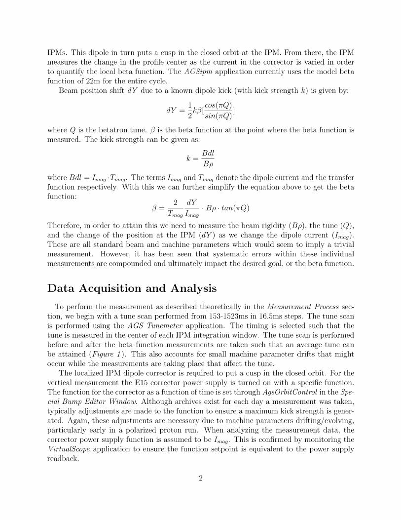
IPMs. This dipole in turn puts a cusp in the closed orbit at the IPM. From there, the IPMmeasures the change in the profile center as the current in the corrector is varied in orderto quantify the local beta function. The AGSipm application currently uses the model betafunction of 22m for the entire cycle.

Beam position shift dY due to a known dipole kick (with kick strength k) is given by:

dY =1

2kβ[

cos(πQ)

sin(πQ)]

where Q is the betatron tune. β is the beta function at the point where the beta function ismeasured. The kick strength can be given as:

k =Bdl

Bρ

where Bdl = Imag ·Tmag. The terms Imag and Tmag denote the dipole current and the transferfunction respectively. With this we can further simplify the equation above to get the betafunction:

β =2

Tmag

dY

Imag

·Bρ · tan(πQ)

Therefore, in order to attain this we need to measure the beam rigidity (Bρ), the tune (Q),and the change of the position at the IPM (dY ) as we change the dipole current (Imag).These are all standard beam and machine parameters which would seem to imply a trivialmeasurement. However, it has been seen that systematic errors within these individualmeasurements are compounded and ultimately impact the desired goal, or the beta function.

Data Acquisition and Analysis

To perform the measurement as described theoretically in the Measurement Process sec-tion, we begin with a tune scan performed from 153-1523ms in 16.5ms steps. The tune scanis performed using the AGS Tunemeter application. The timing is selected such that thetune is measured in the center of each IPM integration window. The tune scan is performedbefore and after the beta function measurements are taken such that an average tune canbe attained (Figure 1 ). This also accounts for small machine parameter drifts that mightoccur while the measurements are taking place that affect the tune.

The localized IPM dipole corrector is required to put a cusp in the closed orbit. For thevertical measurement the E15 corrector power supply is turned on with a specific function.The function for the corrector as a function of time is set through AgsOrbitControl in the Spe-cial Bump Editor Window. Although archives exist for each day a measurement was taken,typically adjustments are made to the function to ensure a maximum kick strength is gener-ated. Again, these adjustments are necessary due to machine parameters drifting/evolving,particularly early in a polarized proton run. When analyzing the measurement data, thecorrector power supply function is assumed to be Imag. This is confirmed by monitoring theVirtualScope application to ensure the function setpoint is equivalent to the power supplyreadback.

2

Figure 1: January 31, 2015 - Two tune scans superimposed (top) with the average andstandard deviation for each time measured (bottom). Average tune is used in final betafunction calculation.

The measurement process starts with the original corrector power supply function whichis the maximum positive kick strength. The AGSipm application triggers and archives everyAGS cycle. From here, the original function is scaled by +1

2and the measurements are

repeated. This is done for several iterations at different corrector functions. The minimumnumber of iterations is five and are as follows: original function, original function scaled by+1

2, original function scaled by −1

2, original function scaled by −1, and the function scaled

by 0 (no dipole kick). The IPM center data can be found in a log file and is saved overmany cycles for each corrector configuration for later analysis (Figure 2 ). The last measuredparameter used in the analysis is the beam momentum which is also saved as a log file.

A Matlab program is used for data analysis. This program loads the required log files,makes calculations based on the files loaded, and plots the relevant information in order tounderstand results as well as potential errors in the measurement. The first step observesthe two tune scans that were taken and finds the average and standard deviation of themeasurements. The average tune is the one used to calculate the betas (Figure 1 ). The nextstep plots the loaded beam centroid for each corrector setting. The beam center is plottedwith respect to the time in the cycle and is averaged over many beam cycles as seen in Figure2. The last part prior to the beta function calculation is the IPM centroid response. Here weplot the slope comparing the shift in the measured centroid motion and the relative dipolekick amplitude (Figure 3 ). The slope is found with these comparisons at each correctorfunction and the deviation of the measurement from the calculated slope is later used in theerror bars for the beta function measurement.

3

Figure 2: January 31, 2015 - Beam center position at IPM for different corrector currentfunctions. Data points are averaged over several AGS beam cycles.

Figure 3: January 31, 2015 - IPM centroid response which plots slope comparing the shiftin the measured centroid motion and the relative dipole kick amplitude. This is plotted forevery measured time in the AGS cycle (left). One example can be seen for the measurementat 285ms (right).

With all of these components, we have everything necessary in order to calculate the betafunction. Thus far we have accounted for the beam rigidity, tune, and the change of theposition at the IPM as we change the dipole current. This leads us to the last step which isto calculate the beta function which is demonstrated in Figure 4. As mentioned prior, thediscrepancy between the measured vs. calculated slope plays a key role in determining theerror bars for the beta function measurement. The following section delves into the analysisin the systematic errors from the data acquisition discussed here.

4

Figure 4: January 31, 2015 - Calculated vertical beta function and beam momentum.

Modifications and Procedure Changes

The primary goal for this run, in addition to measuring the beta function, was to under-stand compounded errors and minimize the negative impact on the beta function measure-ment. This was done by responding to past concerns from prior runs and exploring specificaspects of the measurement process.

Hardware and Software Changes

Since last run there were several concerns which had been addressed and have led tonew implementations for Run15. The first concern was the dipole currents. As part of thebeta function measurement, we need the Imag, the dipole current. It had been assumed tobe a known in that whatever the actual current function being sent was the current beingproduced. It was brought to our attention in Run14 that there was a significant amount ofnoise on the readback function for the dipole current. Over the summer, it was found that thisnoise from the reference and readback of the corrector current was from a common groundof both signals. To alleviate this, filters were added to these signals on all dipole correctorsassociated with the IPMs. Once this was done, we were able to sufficiently determine thatthe functions were properly being followed and the current was known. A comparison of thenoisy readback signal before and after the filters were added can be seen in Figure 5.

Another concern that was discussed over the summer was the channel gains within theIPM. If these are not properly calibrated/understood, it could have a significant impact onany measurement utilized by the IPM. The channel gain calibration was done and thesegains were integrated in the IPM data. It turns out, however, that in spite of this, it seems

5

as though the values initially used were not far from the actual values and thus having littleimpact on the beta function measurements.

Figure 5: Comparison between two E15 corrector current function demonstrating the noisereduction from 2014 and 2015. The left image is from 2014 showing excessive noise betweenthe reference (black) and the readback (red) and the right shows the reduced noise in 2015after filters were added. Both images use a corrector current of ‘0A’.

The final concern mentioned here is the matlab code used to generate the beta functionvalues based upon the measured parameters. Until this run, the centroid motion was takenas an average over the whole cycle. Although it sometimes gave reasonable results, there weretimes where the measurements had undesirable results. Over the summer, there were changesmade to the program such that each measured time in the cycle was analyzed individually.Therefore, special care was taken to understand how the centroid was moving with regardsto its time in the AGS cycle. This was proved to be more accurate and consistent with whatthe model deemed to be correct.

With these improvements, it was found early on that the beta function could be measuredreliably and consistently. Therefore, the majority of the run was dedicated to look forunknown pitfalls and make the measurement more robust to compounded flaws.

Vacuum Pressure Effect

A critical part of the beta function measurement is the usage of the AGS IPM. The AGSIPM measures the ions produced as a result of the circulating beam passing through gasin the vacuum chamber. The number of ions produced from collisions with the circulatingbeam is a function of the beam current and the density of the gas. When using protons,the number of ions generated from collisions with residual gas is too small so to increasethe signal size, a controlled leak of CO2 is used to ‘spoil’ the vacuum. (This does not applyto heavy ions since there are generally enough ions produced to measure a good signal–thispaper only focuses on proton beam).

6

Clearly, the vacuum is paramount in generating a proper signal for our measurement. Inthe past, the vacuum was controlled such that it was at the 4E-7 Torr level. However, therewas not extensive work done recently to see if this was adequate enough for our measurement.Could our signal been distorted enough to change the final outcome?

The first iteration of this measurement was done on January 31st. There were twomeasurements made. The first measurement was done in the same fashion as in prior runs.The second measurement spoiled the vacuum further but kept all other parameters the same.This way all other variables were constant in theory.

Figure 6: Beta function comparison with various vacuum pressures. Green trace indicatesmore ‘spoiled’ vacuum than blue trace. Error bars are generated from the spread of themeasured beta and the fitted data (fit attained from 5 individual measurements at variousdipole corrector currents.)

As seen in Figure 6, the results were not resounding. With the exception of a few points,the final beta function measurement remained essentially the same. This would in theoryconfirm that our typical vacuum settings are sufficient for a nominal setup for the betafunction, therefore very little error can be attributed to the vacuum.

However, this run another parameter was varied–the integration window. Although thevacuum held for the default setting of an 8ms integration window, this is not necessarily truefor all integration window settings. This idea was further explored and will be explainedfurther in this tech note.

Tune Measurements

In normal operation, the two kicks of the horizontal and vertical planes in the AGS tuneme-ter are separated by 300 turns. Depending on what plane is the focus, the trigger timingof the tunemeter is varied accordingly. Early in the run there was an instance where the

7

tunemeter was setup to trigger on a time more relevant for the opposite plane of interestfor the beta function measurement. In this instance the measurement took place 300 turnsafter the desired trigger time, which amounts to approximately a 0.8ms delay. This broughtabout a relevant question: how sensitive is the tune measurement and its impact on thebeta function results? This is particularly pertinent when the tunes are driven close to theinteger.

Last year, Leif had given a presentation which further simulated the dependence on thetune with relation to the betatron fractional error. He found that in order to satisfy ourquality ‘benchmark’ of 5% we need a tune error of less than 0.005 for tunes between 8.6 and8.9. This is easily achievable. However, as the tunes approach 9, we need to be an order ofmagnitude better (0.0005) in tune error to still achieve our goal of 5%. This still is possiblebut this becomes increasingly difficult to achieve and one must start to become concernedabout stability. Therefore, with all of this in mind, a .8ms shift in time could potentially bedisastrous for our measurement, due to a significant part of the AGS cycle having a verticaltune above 8.95.

Figure 7: Tune comparison with tunemeter delay (top) and resulting beta function(bottom).

8

The first step was to try and recreate the original findings and compare to see whathappens to the measurement. On January 31st, a beta function measurement was taken.However, there were two different tune scans taken that day–one with the correct tunemetersettings and another with the .8ms delay. All other parameters were kept constant. Theresults are shown in Figure 7.

As indicated in Figure 7, the results are seemingly subtle, but are relevant. When thetunes are high or quickly changing, it seems as though our measurement is more susceptibleto incorrect tunes and thus an incorrect beta function measurement. A seemingly small errorpropagates to become a larger one at the final result.

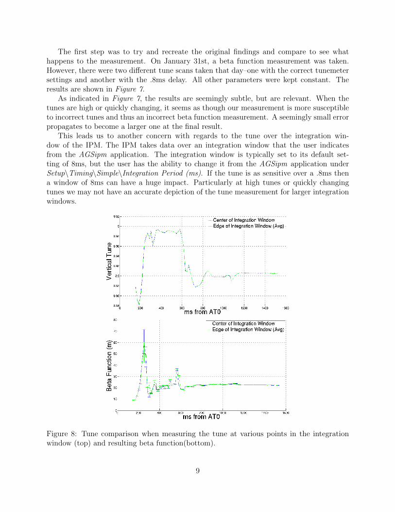
This leads us to another concern with regards to the tune over the integration win-dow of the IPM. The IPM takes data over an integration window that the user indicatesfrom the AGSipm application. The integration window is typically set to its default set-ting of 8ms, but the user has the ability to change it from the AGSipm application underSetup\Timing\Simple\Integration Period (ms). If the tune is as sensitive over a .8ms thena window of 8ms can have a huge impact. Particularly at high tunes or quickly changingtunes we may not have an accurate depiction of the tune measurement for larger integrationwindows.

Figure 8: Tune comparison when measuring the tune at various points in the integrationwindow (top) and resulting beta function(bottom).

9

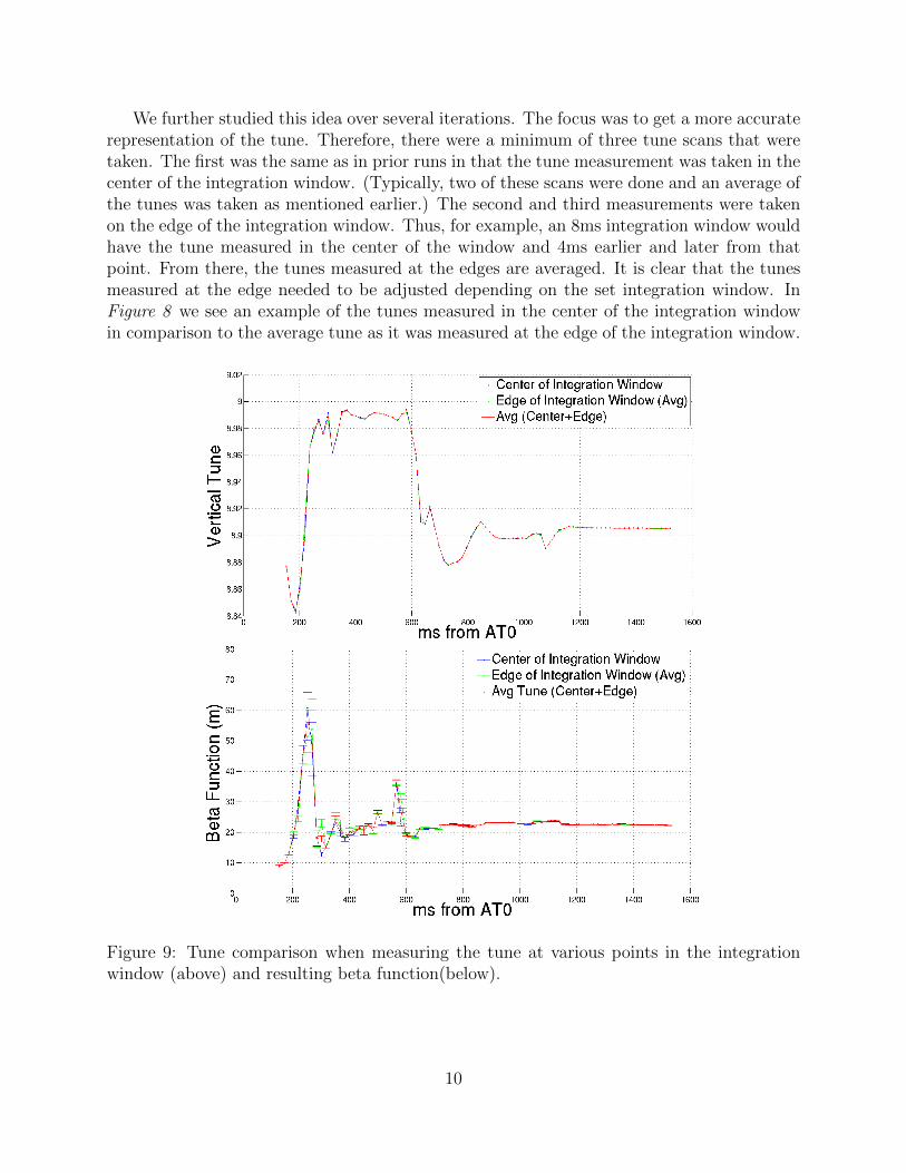
We further studied this idea over several iterations. The focus was to get a more accuraterepresentation of the tune. Therefore, there were a minimum of three tune scans that weretaken. The first was the same as in prior runs in that the tune measurement was taken in thecenter of the integration window. (Typically, two of these scans were done and an average ofthe tunes was taken as mentioned earlier.) The second and third measurements were takenon the edge of the integration window. Thus, for example, an 8ms integration window wouldhave the tune measured in the center of the window and 4ms earlier and later from thatpoint. From there, the tunes measured at the edges are averaged. It is clear that the tunesmeasured at the edge needed to be adjusted depending on the set integration window. InFigure 8 we see an example of the tunes measured in the center of the integration windowin comparison to the average tune as it was measured at the edge of the integration window.

Figure 9: Tune comparison when measuring the tune at various points in the integrationwindow (above) and resulting beta function(below).

10

In the end it was determined that this difference in the timing for the tune measurementwas the most accurate representation of the machine. The tune measured at the centerof the window and the average of the tunes measured at the edge were averaged togetherto generate the tunes used for the beta function measurement. This way, the tunes overthe entire integration window were considered. However, the tune measurements are notweighed the same– by using the central tune and the average of the tunes measured at eachedge, there is more of an emphasis on the tune measured at the center. That is, the tunemeasured at the center is weighted twice as much as each of the edge tunes that contributeto the averaged tune. However, as mentioned before, this is all dependent on the size of theintegration window.

In theory by limiting the size of the window, the tunes should be more accurate andgenerally less fluctuations. In order to truly come to those conclusions we needed to get amore thorough understanding of the integration window in general and the impact it actuallyhas on the beta function measurement.

Integration Window

So up until now we have looked at specific aspects of the beta function measurement.However by looking into these nuances we know that these aspects are further influenced bythe integration window. The integration window, otherwise known as the integration period,is the duration that the analog integrators in the IPM integrate the charge. Therefore, thelonger the integration period, the more fluctuations could take place during the measurement.Thus it is clear that we need to find the optimal setting in order to capitalize on all aspectsof the beta function measurement.

The first instance of this was looking at the impact the window had on the tune mea-surement. As mentioned earlier, we had seen that the tune measurement is impacted at hightunes and areas where the tune changes quickly. This becomes especially true with longerintegration periods. Therefore, as an attempt to combat this, three tune measurements areused for each beta function measurement. The first measurement is in the center of the in-tegration window and the other two are at the edge of the integration window which in turnis averaged. Obviously, depending upon the integration period size, the tune measurementtimes would need to be adjusted. Ideally, the tunes should remain constant regardless ofwhen they were actually measured. The difference in tune measurements can be observed inFigure 10.

In theory, the shorter the integration window, the more accurate the measurement oughtto be. Since the period in which the charge is being integrated is reduced there is less roomfor fluctuation in the measurement to occur. However, it was found during the first iterationof this that as the integration window got smaller, the worse the measurement got at theend. It was not initially clear as to why this would be until a closer look was done for thesignal on the IPM. Using Logview data, we could see the position of the centroid for each ofthe corrector current setpoints. When comparing these centroids for each of the integration

11

Figure 10: Tune comparison with various integration window lengths (top) and resultingbeta function (bottom).

window settings, there seemed to be a ‘jitter’ that got progressively worse the shorter theperiod became. It was perhaps due to the vacuum not being adjusted in accordance withthe change in the integration window. In spite of the prior findings (mentioned in VacuumPressure Effect section), perhaps the vacuum did have an impact on the final measurement,it just was not clear without the shorter integration window.

This led to the final measurement where the vacuum was varied at three independentintegration window timings: 8ms, 4ms, and 2ms. For each integration window timing threedistinct setpoints were used for the CO2 gas leak: 1100, 1200, and 1300. These settings havean average vacuum pressure of 2.5E-7 Torr, 3.5E-7 Torr, and 4.7E-7 Torr respectively. Theresults for select measurements is seen in Figure 11.

12

Figure 11: Beta function comparison with various vacuum pressures and integration windows.Bottom figure has more ‘spoiled’ vacuum than top figure.

The conclusion is that the longer integration window requires less of the CO2 leak whereasthe shorter integration window requires more CO2 leak (ie more spoiled vacuum). This canbe seen when comparing the integration window with various vacuum settings, the betafunctions tend to agree less and less as the leak gets higher for 8ms, yet better with the 2ms.This cannot be said with concrete evidence however, and more measurements would need tobe taken in the future where the vacuum is spoiled further. As of now, it would appear asthough any integration window is valid for this measurement as long as the vacuum pressurewas adequate. At this time, the longer integration window is the most stable due to bettercontrol of the vacuum pressure. In the future, with better control of the CO2 leak, a shorterintegration window should be utilized.

With regards to pursuing information on this–after talking with vacuum group personnel,

13

it seems as though there can be some room as far as the vacuum pressure in concerned. Thevacuum valves will close when the pressure goes higher than 5E-6 Torr or if two of the threeion pumps in the loop trip off. Based on logged data, it appears as though ion pumps wererunning whenever the vacuum leak was increased, so this may be the limiting factor.

Looking Forward

Although a lot of ground was covered over Run15, there is still plenty of room for improve-ment. Everything that has been mentioned thus far has taken place with the vertical ionIPM located at E15. In the future we hope to expand our knowledge of local beta functionmeasurements at other IPMs. In this section we delve into the various other areas whereimprovement can be made.

Horizontal Ion IPM

To date, there has yet to be a successful horizontal beta function measurement using theion IPM at C05 for the entire duration of the AGS cycle. The only section of the cyclethat has been successfully completed is at flattop. It was discovered in Run14 that despitethe deliberate attempt to move the orbit at injection or up the ramp at C05, it seemed asthough the orbit held steady. This is due to the corrector’s close proximity to the RF PUE’sat sections B18 and C12. Since the radial loop is used early on in the AGS cycle, whenevera distortion was made in the orbit between these PUE’s, the average orbit would be movedto compensate for these changes. This unfortunately would distort any measurement thatwas made.

However, while at flattop, the phase loop is used and the distortions made in the orbitby C05 were unperturbed. Therefore adequate measurements were made and thus far haveagreed with the model. However, it would be interesting to get data somewhere other thanat flattop.

There has been some discussion with regards to getting information about the betafunction up the ramp. It would be possible to work with LLRF personnel in order to find aworkaround. It seems unlikely that a whole cycle can be attained like it has for E15. Theidea is that the phase loop could be used for certain parts of the cycle that are not necessarilytypical, however this may not be possible in certain areas (ie transition). This will need tobe further explored in subsequent runs.

eIPMs

There is a horizontal eIPM at D05 and a vertical eIPM at D15. With regards to the betafunction measurements, little work was done with the eIPM’s this run. Although resultswere capable to be generated, there is little agreement between various measurements oreven the model. Predominantly, this is attributed to this being a new system which was stillbeing commissioned–it may not have been configured correctly quite yet.

14

During the shutdown between Run14 and Run15, there was work done on the dipolecorrector power supplies for both D05 and D15. After the upgrades the supplies were capableof ramping from 0A to 12A in 35ms, whereas in Run14, the same thing would require 100ms.In addition, adjustments were made such that the maximum current attainable was 20A.This held true for functions loaded for D15, however, there were several instances where D05dipole corrector would trip due to the current function being too steep, in spite of the factthat it followed the power supply specifications.

The burning question is why the measurements did not agree, neither with each other orwith the model. There are currently some theories which give us some insight. One thoughtis that the transfer function for the power supplies is not correct. Although this would notexplain why the measurements don’t agree, it would explain how nothing thus far agrees withthe model, and the fact that current measurements are approximately a factor of two toolarge. In addition, channel gains had not been calibrated prior to most of the measurements.We are particularly sensitive to this and, again, this does not explain the discrepancy inmeasurements, it is another contributing factor when comparing this to model data. Withregards to the different measurements it appears that all aspects of the measurements areequivalent except for the corrector currents (and thus the orbit). Repeatability should be agoal for subsequent runs to further diagnose this particular issue.

Conclusion

For the duration of Run15 the vertical beta function at E15 IPM was extensively measured.During this time several parameters were scanned. The vacuum leak and integration windowwas varied for the beta function measurement. In the range we changed these parameters,the beta function results did not change much. Nevertheless, a shorter integration windowwith higher gas leak seems to be the natural choice. The effect of the betatron tune duringthe integration window was also studied. It is important, and could have significant effecton the beta function measurement. The average of several tune measurements along theintegration window seems to be the valid one. In Figure 12, we demonstrate the optimizedmeasurement and compared the results with the AGS model. In Table 1, a detailed lookof each individual point is demonstrated. Going forward, there will be dedicated time tounderstand the horizontal beta function (C05) and the use of eIPMs (D05 and D15).

15

Figure 12: Beta function comparison between data taken from April 9th and the model. Topone includes points at 0+, bottom one does not–the model does not include these points asthey do not converge.

16

Table 1: Detailed measurements for each point as gathered from Figure 12.

Time(ms fromAT0)

Beta Error Time(ms fromAT0)

Beta Error

153 9.075 0.508 846 22.442 0.118170 9.752 0.298 863 22.370 0.058186 10.980 0.297 879 22.402 0.045203 16.187 0.488 896 22.502 0.085219 24.176 0.864 912 23.069 0.069236 40.062 4.186 929 23.162 0.037252 51.879 7.931 945 22.884 0.052269 60.346 7.959 962 22.630 0.113285 26.487 1.890 978 23.047 0.228302 21.271 2.018 995 23.001 0.166318 14.524 0.752 1011 23.069 0.130335 20.264 0.313 1028 22.670 0.193351 27.570 0.191 1044 22.893 0.174368 26.309 0.380 1061 23.330 0.123384 19.410 0.367 1077 22.977 0.102401 22.563 0.253 1094 23.395 0.176417 21.742 0.213 1110 23.446 0.225434 22.198 0.144 1127 23.467 0.132450 23.846 0.116 1143 22.792 0.075467 23.862 0.259 1160 22.547 0.069483 23.158 0.114 1176 22.622 0.027500 27.951 0.229 1193 22.819 0.057516 22.428 0.398 1209 22.575 0.134533 22.893 0.197 1226 22.560 0.099549 23.459 0.276 1242 22.634 0.119566 24.522 0.311 1259 22.592 0.113582 19.162 0.134 1275 22.634 0.113599 21.266 0.270 1292 22.524 0.102615 17.800 0.243 1308 22.540 0.084632 19.333 0.177 1325 22.680 0.109648 20.814 0.093 1341 22.663 0.076665 22.221 0.102 1358 22.387 0.115681 23.053 0.181 1374 22.490 0.081698 22.549 0.233 1391 22.519 0.085714 22.821 0.297 1407 22.750 0.087731 23.686 0.180 1424 22.639 0.056747 23.755 0.064 1440 22.484 0.110764 23.893 0.048 1457 22.521 0.062780 23.006 0.071 1473 22.743 0.048797 23.008 0.053 1490 22.546 0.089813 22.374 0.061 1506 22.378 0.074830 22.155 0.093 1523 22.530 0.076

17

References

[1] H. Weisberg et al., Proc. of PAC’83, p.2179.

[2] H. Huang et al., Proc. of IBIC2013, p.492.

[3] R. Connolly, et al., Proc. of IBIC2014, p.39.

18