AIR BEARINGKINEMATIC COUPLING

By

VADIM JACOB TYMIANSKI

A THESIS PRESENTED TO THE GRADUATE SCHOOLOF THE UNIVERSITY OF FLORIDA IN PARTIAL FULFILLMENT

OF THE REQUIREMENTS FOR THE DEGREE OFMASTER OF SCIENCE

UNIVERSITY OF FLORIDA

2006

Copyright 2006

by

Vadim Jacob Tymianski

This work is dedicated to my parents Jacob R. Tymianski and Natalya N.

Viranovskaya.

ACKNOWLEDGMENTS

My advisor, Dr. John Ziegert, is instrumental in guiding this project to a

successful completion. His insight and expertise in the field of precision design and

metrology are invaluable. As well, my gratitude is extended to fellow graduate

students Chi-Hung Cheng, Abhijit Bhattacharyya and Scott Payne for providing

creative input and objective criticism.

iv

TABLE OF CONTENTS

page

ACKNOWLEDGMENTS . . . . . . . . . . . . . . . . . . . . . . . . . . . . . iv

LIST OF FIGURES . . . . . . . . . . . . . . . . . . . . . . . . . . . . . . . . vii

ABSTRACT . . . . . . . . . . . . . . . . . . . . . . . . . . . . . . . . . . . . ix

CHAPTER

1 AIR BEARING KINEMATIC COUPLING . . . . . . . . . . . . . . . . 1

1.1 Introduction . . . . . . . . . . . . . . . . . . . . . . . . . . . . . . . 11.2 Motivating Need for Repeatability . . . . . . . . . . . . . . . . . . . 41.3 Kinematic Coupling Concept . . . . . . . . . . . . . . . . . . . . . . 41.4 Research Goals . . . . . . . . . . . . . . . . . . . . . . . . . . . . . 4

2 CURRENT STATE OF THE ART . . . . . . . . . . . . . . . . . . . . . 6

2.1 Literature Review . . . . . . . . . . . . . . . . . . . . . . . . . . . . 62.2 Commercial Couplings . . . . . . . . . . . . . . . . . . . . . . . . . 8

3 CONCEPTUAL DESIGN OF ABKC . . . . . . . . . . . . . . . . . . . . 9

3.1 Component Layout . . . . . . . . . . . . . . . . . . . . . . . . . . . 93.2 Automated Testing . . . . . . . . . . . . . . . . . . . . . . . . . . . 10

4 KINEMATIC ANALYSIS . . . . . . . . . . . . . . . . . . . . . . . . . . 12

4.1 Spatial Geometry . . . . . . . . . . . . . . . . . . . . . . . . . . . . 124.2 Kinematics . . . . . . . . . . . . . . . . . . . . . . . . . . . . . . . 134.3 Global Stiffness . . . . . . . . . . . . . . . . . . . . . . . . . . . . . 17

5 SYSTEM COMPONENTS . . . . . . . . . . . . . . . . . . . . . . . . . . 23

5.1 Base . . . . . . . . . . . . . . . . . . . . . . . . . . . . . . . . . . . 235.2 Top . . . . . . . . . . . . . . . . . . . . . . . . . . . . . . . . . . . . 245.3 Damper . . . . . . . . . . . . . . . . . . . . . . . . . . . . . . . . . 245.4 Air Bearing . . . . . . . . . . . . . . . . . . . . . . . . . . . . . . . 255.5 Capacitance Probe Holder . . . . . . . . . . . . . . . . . . . . . . . 265.6 Electro-Mechanical System . . . . . . . . . . . . . . . . . . . . . . . 265.7 Data Aquisition System . . . . . . . . . . . . . . . . . . . . . . . . 27

v

6 TEST RESULTS . . . . . . . . . . . . . . . . . . . . . . . . . . . . . . . 30

6.1 Test Configurations . . . . . . . . . . . . . . . . . . . . . . . . . . . 306.2 Drift Test . . . . . . . . . . . . . . . . . . . . . . . . . . . . . . . . 306.3 No Float . . . . . . . . . . . . . . . . . . . . . . . . . . . . . . . . . 33

6.3.1 Repeatability . . . . . . . . . . . . . . . . . . . . . . . . . . 336.3.2 Impact . . . . . . . . . . . . . . . . . . . . . . . . . . . . . . 34

6.4 Half Float . . . . . . . . . . . . . . . . . . . . . . . . . . . . . . . . 356.5 Full Float . . . . . . . . . . . . . . . . . . . . . . . . . . . . . . . . 36

6.5.1 Repeatability . . . . . . . . . . . . . . . . . . . . . . . . . . 366.5.2 Impact . . . . . . . . . . . . . . . . . . . . . . . . . . . . . . 38

6.6 Solid Sphere Contact . . . . . . . . . . . . . . . . . . . . . . . . . . 406.6.1 Repeatability . . . . . . . . . . . . . . . . . . . . . . . . . . 406.6.2 Impact . . . . . . . . . . . . . . . . . . . . . . . . . . . . . . 41

7 CONCLUSIONS . . . . . . . . . . . . . . . . . . . . . . . . . . . . . . . 44

APPENDIX

COMPONENT DRAWINGS . . . . . . . . . . . . . . . . . . . . . . . . 45

REFERENCES . . . . . . . . . . . . . . . . . . . . . . . . . . . . . . . . . . . 51

BIOGRAPHICAL SKETCH . . . . . . . . . . . . . . . . . . . . . . . . . . . . 53

vi

LIST OF FIGURES

Figure page

1–1 Cartesian degrees of freedom . . . . . . . . . . . . . . . . . . . . . . . . . 1

1–2 Conventional kinematic coupling using 3 balls mated into 3 v-grooves . . 2

3–1 Air bearing degrees of freedom . . . . . . . . . . . . . . . . . . . . . . . . 9

4–1 Plucker line in space and its defining vectors . . . . . . . . . . . . . . . . 12

4–2 Air bearing directions . . . . . . . . . . . . . . . . . . . . . . . . . . . . 14

4–3 Coordinate systems . . . . . . . . . . . . . . . . . . . . . . . . . . . . . . 16

4–4 Capacitance probe orientation . . . . . . . . . . . . . . . . . . . . . . . . 17

4–5 Hertzian . . . . . . . . . . . . . . . . . . . . . . . . . . . . . . . . . . . . 18

4–6 Loading envelope of ABKC. X and Y are in meters while Z is nondimensional stiffness. Uniformity of top surface signifies that stiffness ofan ABKC does not significantly inside the loading envilope. . . . . . . . 22

5–1 Bearing stacks on base . . . . . . . . . . . . . . . . . . . . . . . . . . . . 23

5–2 Top . . . . . . . . . . . . . . . . . . . . . . . . . . . . . . . . . . . . . . 24

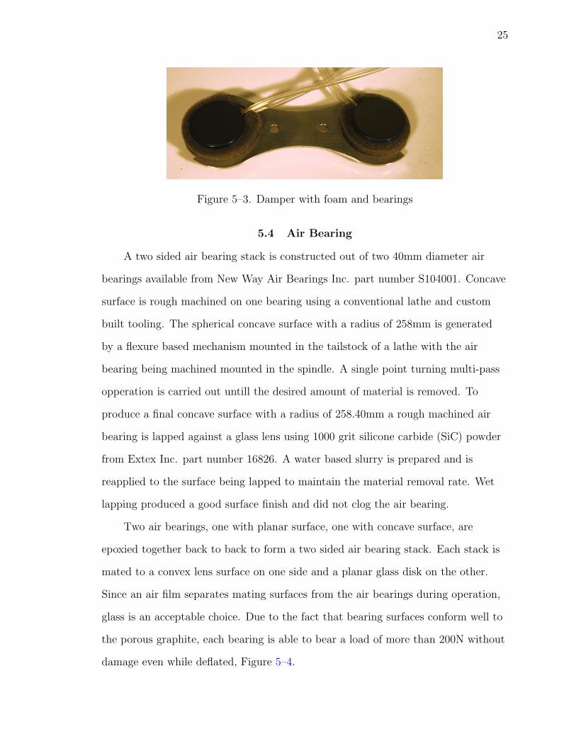
5–3 Damper with foam and bearings . . . . . . . . . . . . . . . . . . . . . . . 25

5–4 Double sided air bearings with manifold . . . . . . . . . . . . . . . . . . 26

5–5 Capacitance probe holder . . . . . . . . . . . . . . . . . . . . . . . . . . 27

5–6 Control board . . . . . . . . . . . . . . . . . . . . . . . . . . . . . . . . . 28

5–7 Experimental setup . . . . . . . . . . . . . . . . . . . . . . . . . . . . . . 29

6–1 Capacitance probe drift test . . . . . . . . . . . . . . . . . . . . . . . . . 31

6–2 Drift test histogram . . . . . . . . . . . . . . . . . . . . . . . . . . . . . 31

6–3 Drift test record and ensemble averages . . . . . . . . . . . . . . . . . . . 32

6–4 Autocorrelation of drift test signal . . . . . . . . . . . . . . . . . . . . . 33

6–5 Direct reading of six cap probes . . . . . . . . . . . . . . . . . . . . . . . 33

vii

6–6 Transformed components of cartesian motion . . . . . . . . . . . . . . . . 34

6–7 No float load curve . . . . . . . . . . . . . . . . . . . . . . . . . . . . . . 34

6–8 No float FRF . . . . . . . . . . . . . . . . . . . . . . . . . . . . . . . . . 35

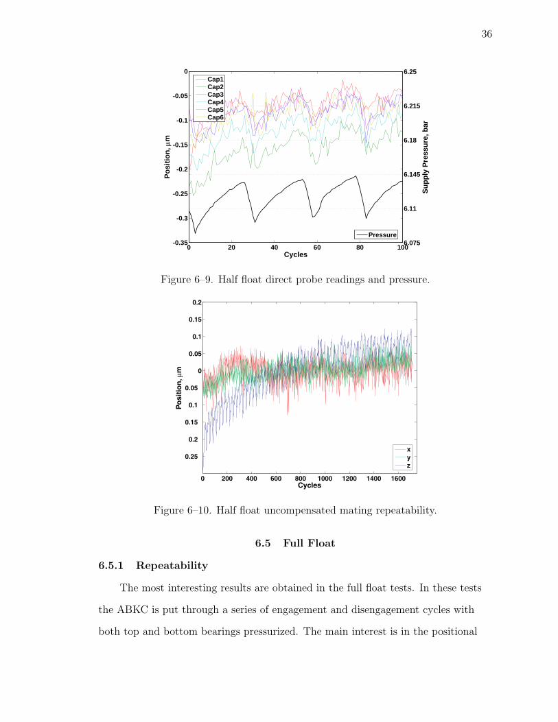
6–9 Half float direct probe readings and pressure. . . . . . . . . . . . . . . . 36

6–10 Half float uncompensated mating repeatability. . . . . . . . . . . . . . . 36

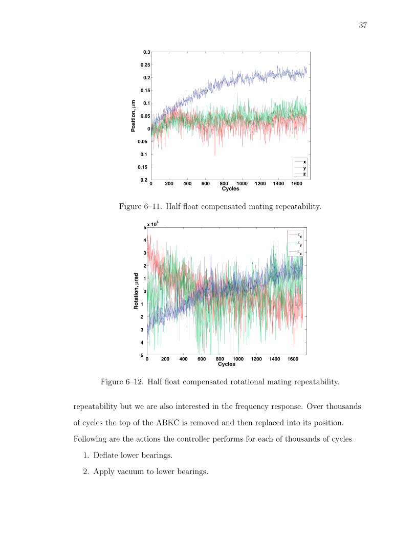
6–11 Half float compensated mating repeatability. . . . . . . . . . . . . . . . . 37

6–12 Half float compensated rotational mating repeatability. . . . . . . . . . . 37

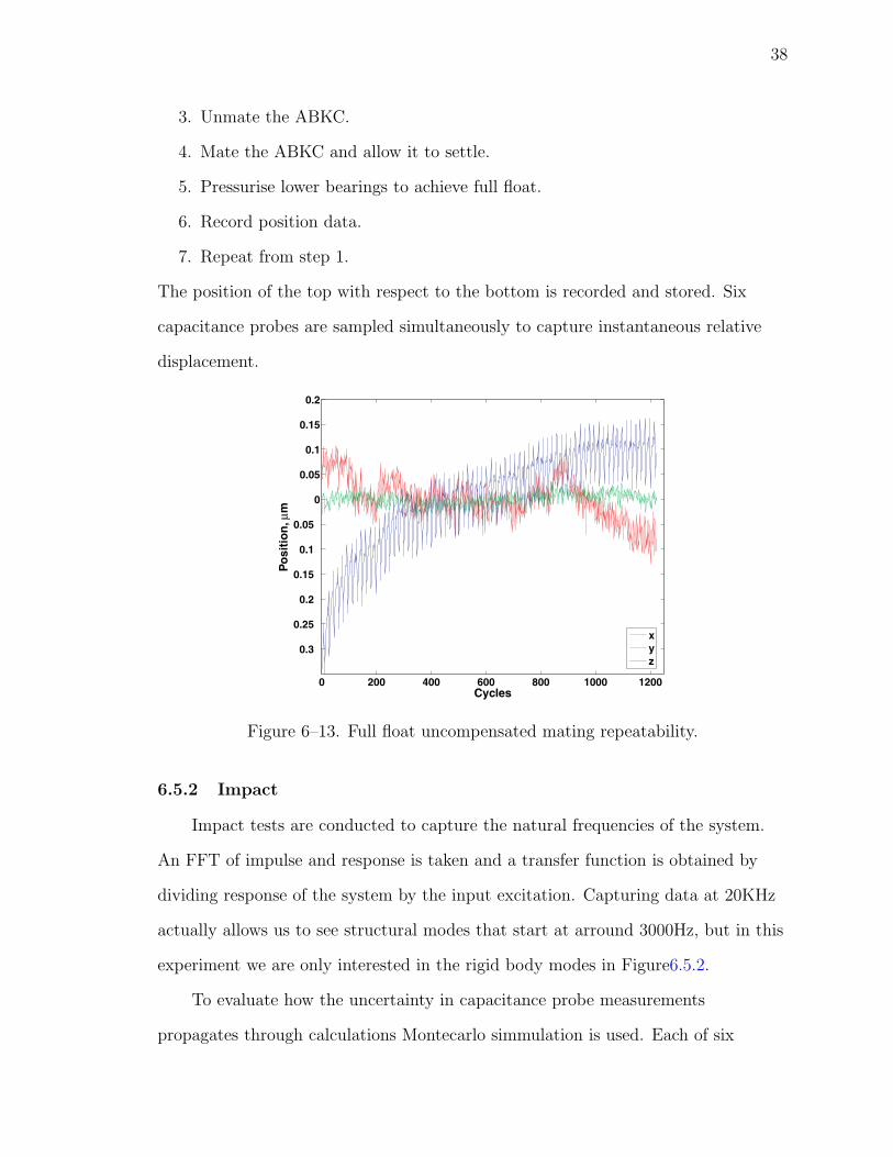
6–13 Full float uncompensated mating repeatability. . . . . . . . . . . . . . . . 38

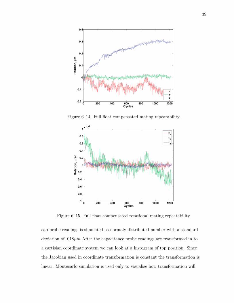
6–14 Full float compensated mating repeatability. . . . . . . . . . . . . . . . . 39

6–15 Full float compensated rotational mating repeatability. . . . . . . . . . . 39

6–16 FRF of a fully floated ABKC . . . . . . . . . . . . . . . . . . . . . . . . 40

6–17 Transformation histograms . . . . . . . . . . . . . . . . . . . . . . . . . . 41

6–18 ABKC converted to ball flat configuration . . . . . . . . . . . . . . . . . 41

6–19 Stiction resulting in inability of conventional coupling to mate. . . . . . . 42

6–20 Ball flat contact FRF. . . . . . . . . . . . . . . . . . . . . . . . . . . . . 42

6–21 Load testing of ABKC . . . . . . . . . . . . . . . . . . . . . . . . . . . . 42

6–22 Load curve . . . . . . . . . . . . . . . . . . . . . . . . . . . . . . . . . . 43

viii

Abstract of Thesis Presented to the Graduate Schoolof the University of Florida in Partial Fulfillment of the

Requirements for the Degree of Master of Science

AIR BEARINGKINEMATIC COUPLING

By

Vadim Jacob Tymianski

August 2006

Chair: John ZiegertMajor Department: Mechanical and Aerospace Engineering

The ”kinematic coupling” is a well known device used to achieve highly

repeatable positioning of one machine or instrument element relative to another.

Normally it consists of 3 precision balls attached to the first mating element in a

triangular pattern. These balls mate with 3 v-grooves in the surface of the second

mating element, creating six ball-on-flat point contacts between bodies. Ideally this

arrangement would result in mating repeatability of the same order as the surface

roughness of balls and v-grooves. In reality, friction forces at the contact points

limit the repeatability and accuracy of the coupling and can result in wear over

time. This paper describes a novel air bearing kinematic coupling (ABKC) design

where ball-on-flat contacts are replaced with intermediate elements consisting of

double-sided porous carbon air bearings. Air bearings are designed with one planar

surface and one concave spherical surface so that an individual air bearing restricts

only a single degree of freedom. Each double sided air bearing stack exhibits

stiffness only in the axial direction when loaded. When six of such air bearing

stack elements are placed at the appropriate locations between mating bodies, they

will fully constrain motion of one body with respect to another. Overconstraint

ix

is eliminated and mating repeatability is improved as compared to solid contact

kinematic couplings due to elimination of friction and wear at the constraints.

x

CHAPTER 1AIR BEARING KINEMATIC COUPLING

1.1 Introduction

This thesis describes the concept, design, manufacturing and testing of a

novel kinematic coupling. Porous carbon air bearings are used as mating elements

between the top and bottom parts of a coupling. This thesis encompasses all issues

as well as their resolutions, encountered in the process of Air Bearing Kinematic

Coupling (ABKC) development.

The kinematic coupling is a well known and widely used device for providing

highly repeatable positioning of one machine or instrument element relative to

another. In general, instrument elements or even whole machines can be thought of

as rigid bodies located in space. Each body has six degrees of freedom that define

its position and orientation in Cartesian space; three translational - X, Y , Z and

three rotational - θx, θy, θz.

Figure 1–1. Cartesian degrees of freedom

In order to locate or constrain one body with respect to the other the above

listed six degrees of freedom need to be constrained. The desired approach is to

1

2

constrain exactly six degree of freedom independently without over constraining

the bodies. This is the area where kinematic couplings offer several benefits. In

the common ball and v-groove coupling, the two bodies make contact at six points.

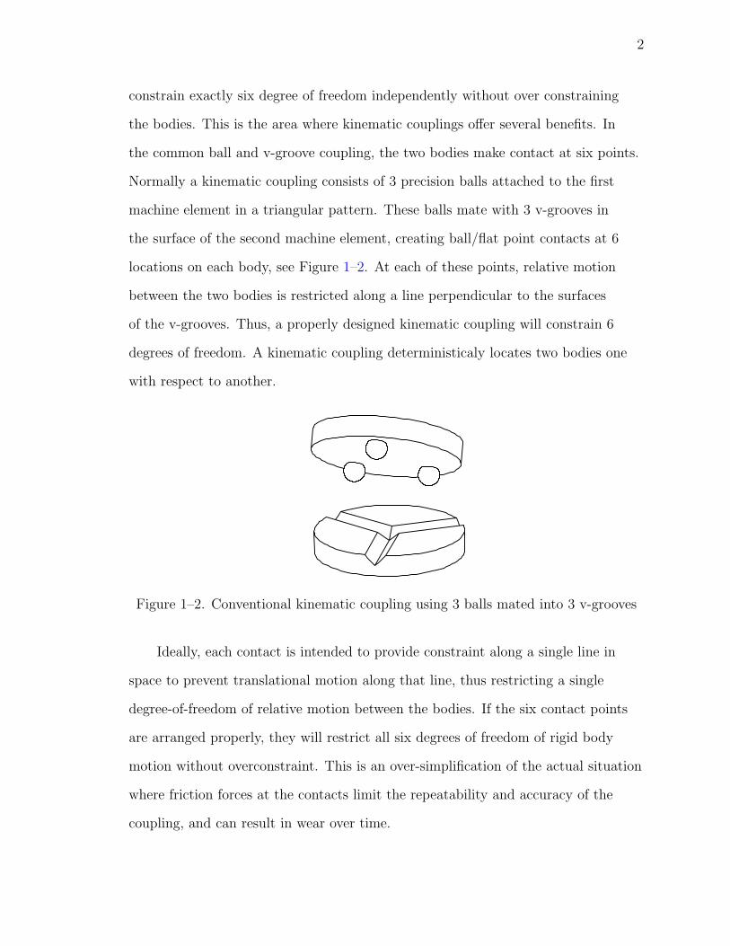
Normally a kinematic coupling consists of 3 precision balls attached to the first

machine element in a triangular pattern. These balls mate with 3 v-grooves in

the surface of the second machine element, creating ball/flat point contacts at 6

locations on each body, see Figure 1–2. At each of these points, relative motion

between the two bodies is restricted along a line perpendicular to the surfaces

of the v-grooves. Thus, a properly designed kinematic coupling will constrain 6

degrees of freedom. A kinematic coupling deterministicaly locates two bodies one

with respect to another.

Figure 1–2. Conventional kinematic coupling using 3 balls mated into 3 v-grooves

Ideally, each contact is intended to provide constraint along a single line in

space to prevent translational motion along that line, thus restricting a single

degree-of-freedom of relative motion between the bodies. If the six contact points

are arranged properly, they will restrict all six degrees of freedom of rigid body

motion without overconstraint. This is an over-simplification of the actual situation

where friction forces at the contacts limit the repeatability and accuracy of the

coupling, and can result in wear over time.

3

Solid contact kinematic couplings are inherently limited in performance

by parasitic frictional forces. In machine and instrument construction the most

common way of interfacing two bodies is through an area contact, which provides

high stiffness and load capacity. When preloaded, these contacts resist relative

motion of the bodies through friction. One of the flaws of the area contact is its

low repeatability in mating. When two bodies are mated they should settle into

a lowest energy state. This would result in a stable equilibrium, and an increase

in mating force should not produce any relative motion between bodies. In area

contact, frictional force arises as soon as there is physical contact and will oppose

relative motion between bodies towards an energetically stable configuration.

Current solid contact kinematic couplings consist of mating elements that

behave as area contacts as the load increases, and the positioning repeatability

performance is reduced by friction.

In this paper a novel kinematic coupling is described where the ball-flat

contacts are replaced by double sided porous carbon air bearings designed to

restrict relative motion along a single line in space while providing virtually zero

friction forces in all other directions. An air bearing stack is constructed in such

a way as to constrain only one degree of freedom. By using six of the air bearing

stacks assembled in a non-singular configuration a kinematic coupling is formed.

At zero relative velocity air bearings provide an almost frictionless contact between

mating bodies. Absence of the frictional force allows a much better repeatability

than solid contact kinematic couplings.

It is known that air bearings operated with gaps on the order of 5− 25µm can

exhibit stiffness on the same order of magnitude as Hertzian contacts in ball-flat

pairs, but are capable of carrying much higher loads, thus giving the ABKC the

potential to carry larger loads than an equivalently sized ball-flat coupling. In the

following sections the design of the ABKC, modeling of its kinematic behavior,

4

and experimental data for coupling repeatability, stiffness, and load capacity

are described. Film thickness dependence on air supply pressure and preload

is investigated, as well as the resulting impact on coupling stiffness. Different

configurations of the coupling are also tested.

1.2 Motivating Need for Repeatability

Technological advances continuously demand higher and higher levels of

mechanical accuracy. While efficient active compensation schemes for improved

precision do exist, mechanical precision is still fundamentally important. Precision

assembly is critical on both ends of the instrument size scale. From MEMS

assembly to large telescope mirror positioning, repeatable mating of machine

components is crucial.

1.3 Kinematic Coupling Concept

Using a kinematic coupling as an interface between two bodies allows

for a certain degree of repeatability to be maintained through many

engagement-disengagement cycles. The concept of kinematic coupling and

kinematic constraint has been known and used for a long time. When two bodies

are connected through a kinematic coupling several benefits are realized. Thermally

induced dimensional changes are accommodated and do not cause internal stresses.

Also, components can be of lower accuracy and lower cost while still maintaining

highly precise positioning. Components interfaced through kinematic couplings can

be moved and later be placed back to the original position with high repeatability

without expensive active position feedback devices.

1.4 Research Goals

One of the main goals of this research is to determine the performance

parameters of an ABKC. The mating repeatability is of primary interest. If the

ABKC is to be successfuly used in the future many other operating parameters

need to be quantified. Static and dynamic stiffnesses are very important

5

parameters when describing a coupling. Static stiffness determines deflection

under load while dynamic stiffness characterizes the response of a coupling to

impact or vibratory disturbances. Individual air bearing stiffness greatly varies

with air film thickness, and in turn is dependent on supply air pressure.

Conventional kinematic couplings have very low damping and do not provide

substantial vibration damping and isolation characteristics. Impact testing is

performed to determine how much damping an ABKC has.

Solid contact kinematic couplings suffer the degradation in performance from

wear associated with repeated mating of tribological surfaces. Experimentaly it is

possible to determine if the problem of surface wear can be mitigated by air film

between an air bearing and surface it rests against.

CHAPTER 2CURRENT STATE OF THE ART

2.1 Literature Review

The mechanics and performance of kinematic couplings have been studied

extensively by many authors [1-13]. In general, a coupling can be analysed using

the vector method outlined in Schmiechen and Slocum [7]. This approach to

the analysis of kinematic systems reduces to matrix analysis. Two characteristic

assumptions are made in this analysis: 1. error motions are small and 2. all

deformation occurs at the contact points. These simplifying assumptions allow

inclusion of friction at point contacts in the model. Summing up friction force

and Hertzian contact force produces a resultant that is not normal to the contact

surface. This requires a change of system matrix and use of modified Hertzian

stress calculations for oblique contacts.

Culpepper et al. [4] report on the design and construction of the prototype

actuated coupling allowing position adjustment in 6-DOF. A kinematic model for

an eccentric ball-shaft actuation is developed and prototype performance matches

this model within 10 %. In the experiment balls and grooves are made from 304L

stainless and are protected by a 3.5µm TiN coating and high-pressure grease. Over

the course of more than 500 engagements stabilized 1σ repeatability of better than

1.9µm and 3.6µrad was reported. However, friction at the contact points did not

allow the couplings to be adjusted while mated and loaded. Authors assume that

short wear in period of 50 cycle is perhaps indicative of grease being displaced from

the contact and not tribological wear of the surfaces.

Earlier investigations by Slocum and Donmez are presented in a two part

article [9] and [10] describe design and testing of a ball-flat coupling with a 45kN

6

7

preload constructed with ceramic balls. During testing 3σ repeatability of 0.3µm

was achieved.

For non-actuated, conventional kinematic couplings repeatability of 0.1µm is

possible [8]. Such high level of repeatability is possible for a period of time after

the wear-in and before the degradation of performance due to burnishing from

further mating and wear at the contacts. The number of engagements possible at

such a high level of repeatability depends on the ball-flat material but will allways

degrade with repeated mating. Polished, ceramic surfaces have particularly good

performance in terms of wear.

One of the advantages of a kinematic coupling is its ability to center itself or

come to the minimal potential energy state. Solid contact couplings are not all

self-centering. For some configurations there exist a critical coefficient of friction

for the ball-flat interface. If it is exceeded, the coupling will not self-center under a

steady preload without intervention and manual adjustment.

In summary, various implementations of the kinematic coupling concept have

been developed over the years. Overall performance of an individual coupling is

determined by several design constraints such as: load bearing capacity, spatial

constraints, contact pair orientation and material. Adjustable kinematic couplings

are subject to the same performance limiting factors. The most significant of

them is friction. Mechanical assembly accuracy is inherently limited by friction

and hysteresis. Wear is an issue with high accuracy surfaces. During mating the

order in which contacting pairs are brought in to contact influences repeatability.

Ideally each contact pair would restrict only one DOF that is normal to contacting

surfaces but it is not the case. Once contacting surfaces are brought in to contact

parasitic frictional forces arise. These forces resist settlement of a coupling into a

lowest energy state and degrade repeatability. Another limitation of traditional

kinematic couplings is their relatively low load carrying capacity. All of the applied

8

load must be carried via Hertzian contacts which results in very high stresses and

the potential for plastic deformation at the contact points, further reducing the

repeatability of the device.

2.2 Commercial Couplings

Most kinematic couplings sold are integrated into the larger mechanism. For

example large mirror segments in the oplical telescopes are held in a structure

called ’wiffle tree’ which is essentially a series of kinematic couplings arranged as

a pyramid. Such an arrangement allows for accomodation of thermal expansion of

individual mirror segments without straining the whole mirror assembly.

Another application is in the support of granite bases of coordinate

measurement machines and granite optical tables. Even large diamond turning

machines are kinematicaly supported.

What is widely available in the marketplace is individual coupling components

such as polished spheres made from hard steel or ceramic and hardened flats. It is

left up to the designer to pick appropritae mating elements and to determine their

arrangement.

CHAPTER 3CONCEPTUAL DESIGN OF ABKC

3.1 Component Layout

The geometric arrangement of air bearing stacks in an ABKC is one of the

most important factors determining its performance. Bearing stack orientation

has direct influence on the stiffness, repeatability and directional range in which a

coupling can be loaded. In the layout chosen ABKC bearing stacks are placed in

pairs on mutually perpendicular faces.

Each air bearing stack allows free rotation about all 3 coordinate axes and free

translation in 2 directions only restricting one DOF, see Figure 3–1. In other words

air bearing stack is only stiff in Z directon. Placing two bearings on one face allows

the constraint of one translational and one rotational DOF. Since pairs of bearings

are located on three mutually perpendicular faces of the base, three translational

and tree rotational DOF are constrained.

Figure 3–1. Air bearing degrees of freedom

9

10

In order to monitor the position of the top with respect to bottom it is needed

to measure six independent linear displacements. The most convenient non-contact

method is capacitive sensing. This method measures the capacitance of an electic

field between the probe and the target. As distance between probe and target

changes so does the capacitance. A resonating RC circuit is used to track changes

in capacitance and a microprocessor is used to convert capacitance changes in to

distance changes.

Reading rotational displacement is more difficult with non-contact methods.

That is why six linear displacements are measured and later converted into three

cartesian motions and three rotations around mutually perpendicular axes. If six

capacitance probes are located on the base with their axies parallel to the axes of

air bearing stacks two benefits are realized. First, direct capacitance probe readings

provide measurement of the air gap variation of individual bearing stacks. Second,

direct readings are transformed to provide cartesian displacements and rotations.

Individual components will be described in more detail in Chapter 5.

3.2 Automated Testing

Forseing a large ammount of testing that ABKC is to undergo it is designed

to be automated. Since reengagement repeatability of thr ABKC is of primary

interest, testing will consist of unmating and mating the top for thousands of

cycles. To minimise the error introduced by a human operator the ABKC is

designed to be fully automated for testing and data aquisition. To obtain data that

is statisticaly meaningful numerous testing scenarios with many engagements of the

ABKC are planned. The actuation system consists of a pneumatic cylinder with a

stroke of 10mm that is computer controlled to provide precise timing and sequence

control during measurements. The position is registered through six channels of

capacitance distance sensors. The performance of air bearings is strongly influenced

11

by air pressure. A pressure transducer is placed close to the air bearings manifold

to record any fluctuations in the supply air pressure.

CHAPTER 4KINEMATIC ANALYSIS

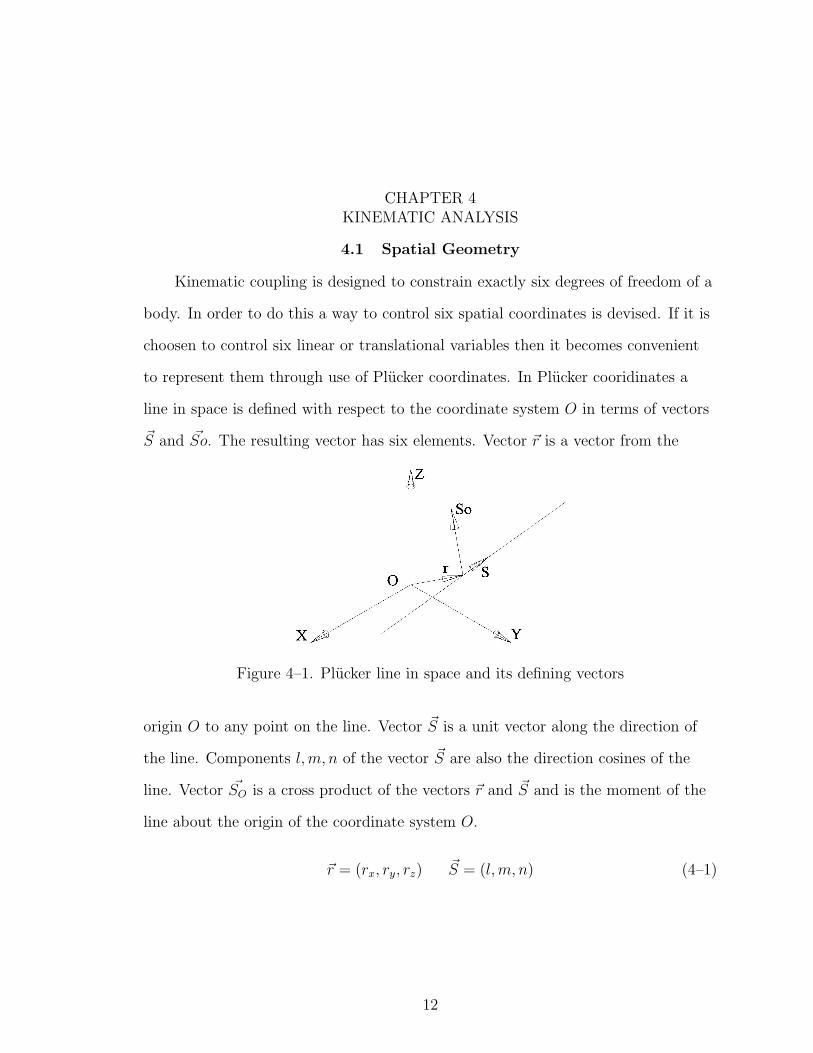
4.1 Spatial Geometry

Kinematic coupling is designed to constrain exactly six degrees of freedom of a

body. In order to do this a way to control six spatial coordinates is devised. If it is

choosen to control six linear or translational variables then it becomes convenient

to represent them through use of Plucker coordinates. In Plucker cooridinates a

line in space is defined with respect to the coordinate system O in terms of vectors

~S and ~So. The resulting vector has six elements. Vector ~r is a vector from the

Figure 4–1. Plucker line in space and its defining vectors

origin O to any point on the line. Vector ~S is a unit vector along the direction of

the line. Components l,m, n of the vector ~S are also the direction cosines of the

line. Vector ~SO is a cross product of the vectors ~r and ~S and is the moment of the

line about the origin of the coordinate system O.

~r = (rx, ry, rz) ~S = (l,m, n) (4–1)

12

13

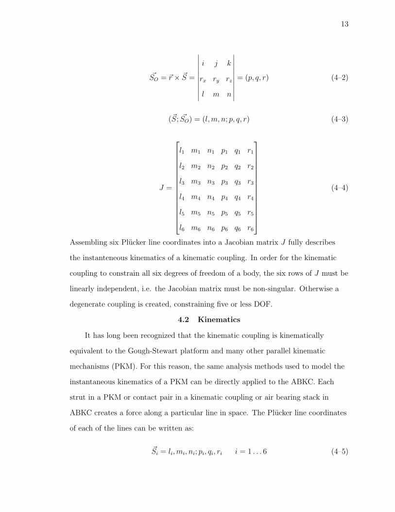
~SO = ~r × ~S =

∣∣∣∣∣∣∣∣∣∣i j k

rx ry rz

l m n

∣∣∣∣∣∣∣∣∣∣= (p, q, r) (4–2)

(~S; ~SO) = (l,m, n; p, q, r) (4–3)

J =

l1 m1 n1 p1 q1 r1

l2 m2 n2 p2 q2 r2

l3 m3 n3 p3 q3 r3

l4 m4 n4 p4 q4 r4

l5 m5 n5 p5 q5 r5

l6 m6 n6 p6 q6 r6

(4–4)

Assembling six Plucker line coordinates into a Jacobian matrix J fully describes

the instanteneous kinematics of a kinematic coupling. In order for the kinematic

coupling to constrain all six degrees of freedom of a body, the six rows of J must be

linearly independent, i.e. the Jacobian matrix must be non-singular. Otherwise a

degenerate coupling is created, constraining five or less DOF.

4.2 Kinematics

It has long been recognized that the kinematic coupling is kinematically

equivalent to the Gough-Stewart platform and many other parallel kinematic

mechanisms (PKM). For this reason, the same analysis methods used to model the

instantaneous kinematics of a PKM can be directly applied to the ABKC. Each

strut in a PKM or contact pair in a kinematic coupling or air bearing stack in

ABKC creates a force along a particular line in space. The Plucker line coordinates

of each of the lines can be written as:

~Si = li, mi, ni; pi, qi, ri i = 1 . . . 6 (4–5)

14

Figure 4–2. Air bearing directions

where: l,m, n are the direction cosines of the line, and p, q, r are the components

of the moment of the line about the origin. The Jacobian matrix of a PKM relates

small motions along the six lines to changes in the position and orientation of the

platform. The rows of the Jacobian matrix are simply the Plucker coordinates of

the six strut axes in a PKM, or the six lines of contact force in ABKC. Therefore,

∆1

∆2

∆3

∆4

∆5

∆6

=

l1 m1 n1 p1 q1 r1

l2 m2 n2 p2 q2 r2

l3 m3 n3 p3 q3 r3

l4 m4 n4 p4 q4 r4

l5 m5 n5 p5 q5 r5

l6 m6 n6 p6 q6 r6

δx

δy

δz

εx

εy

εz

(4–6)

Where: δx, δy, δz are the displacements of a point on the platform which is

instantaneously coincident with the origin of the coordinate system in which

all of the vectors are expressed, εx, εy, εz are rotations of the platform about the

15

coordinate axes, and ∆1 . . . ∆6 are small displacements of the contact point along

the line of force.

The cartesian translations and rotations of the platform relative to the

base, resulting from small changes in displacements along the contact lines, are

obtained using the inverse of the Jacobian. If the device is in a singular position,

the inverse Jacobian does not exist and the systems loses one or more restraints

of degrees of freedom of the platform. For the ABKC described here, there are 2

Jacobian matrices of interest, one for the air bearing stacks (4–7), and one for the

capacitance probes (4–8) that measure relative motions.

Jbearing =

0.7071 0.4082 0.5774 91.3398 −90.6613 −47.7607

0.7071 0.4082 0.5774 32.8451 −124.4333 47.7607

0 −0.8165 0.5774 −124.1849 −33.7719 −47.7607

0 −0.8165 0.5774 −124.1849 33.7719 47.7607

−0.7071 0.4082 0.5774 32.8451 124.4333 −47.7607

−0.7071 0.4082 0.5774 91.3398 90.6613 47.7607

(4–7)

Jcap =

0.7071 0.4082 0.5774 115.4635 −74.5380 −88.7070

0.7071 0.4082 0.5774 5.9043 −147.1041 96.7870

0 −0.8165 0.5774 −122.2835 −62.7253 −88.7070

0 −0.8165 0.5774 −130.3481 68.4387 96.7870

−0.7071 0.4082 0.5774 6.8200 137.2633 −88.7070

−0.7071 0.4082 0.5774 124.4437 78.6654 96.7870

(4–8)

Both Jacobians are expressed relative to a coordinate system O fixed to the

center of the top platform, with the Z-axis perpendicular to the top surface and the

X and Y axes along the top surface, Figure 4.2. Both Jacobians are obtained from

a symbolic tranformation given in (4–9). First coordinate system that is attached

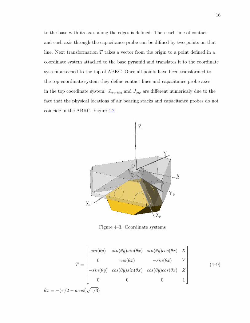
16

to the base with its axes along the edges is defined. Then each line of contact

and each axis through the capacitance probe can be difined by two points on that

line. Next transformation T takes a vector from the origin to a point defined in a

coordinate system attached to the base pyramid and translates it to the coordinate

system attached to the top of ABKC. Once all points have been transformed to

the top coordinate system they define contact lines and capacitance probe axes

in the top coordinate system. Jbearing and Jcap are different numericaly due to the

fact that the physical locations of air bearing stacks and capacitance probes do not

coincide in the ABKC, Figure 4.2.

O

X

Y

Z

P

Xp

Yp

Zp

Figure 4–3. Coordinate systems

T =

sin(θy) sin(θy)sin(θx) sin(θy)cos(θx) X

0 cos(θx) −sin(θx) Y

−sin(θy) cos(θy)sin(θx) cos(θy)cos(θx) Z

0 0 0 1

(4–9)

θx = −(π/2− acos(√

1/3)

17

θy = 3π/4

X = Y = Z = 0.1597m

CenterAxis

CenterAxis

CenterAxis

CenterAxis

CenterAxis

CenterAxis

Figure 4–4. Capacitance probe orientation

4.3 Global Stiffness

Most kinematic couplings are constructed out of six contact pairs. Each

contact pair is usually made up of a ball and flat and sometimes of a cylinder and

cylinder. These arrangements create an interface that most closely resembles a

point contact. Ideally each contact point would be infinitely stiff, but it is not

the case. For solid to solid contact couplings each interface will possess Hertzian

contact stiffness, Eq. 4–10. Each contact pair also transmits forces Fx and Fy as

well as moment Mz.

k =dP

dδ= (6E2PR)

13 where

1

E=

1− ν21

E1

+1− ν22

E2

(4–10)

E is a modulus of elasticity obtained from ball and flat moduli E1 and E2. ν1

and ν2 are Poissons ratios of ball and flat materials. R is ball radius and P is

load. For air bearing stacks used in ABKC the stiffness is obtained experimentally

18

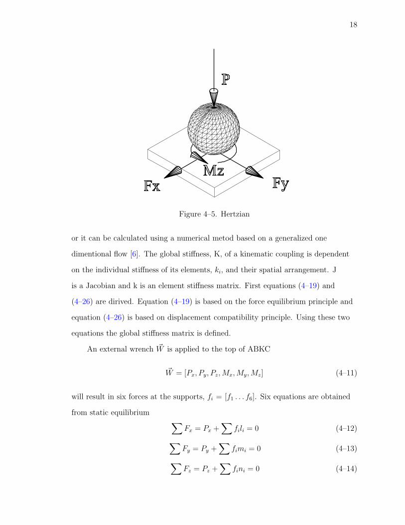
Figure 4–5. Hertzian

or it can be calculated using a numerical metod based on a generalized one

dimentional flow [6]. The global stiffness, K, of a kinematic coupling is dependent

on the individual stiffness of its elements, ki, and their spatial arrangement. J

is a Jacobian and k is an element stiffness matrix. First equations (4–19) and

(4–26) are dirived. Equation (4–19) is based on the force equilibrium principle and

equation (4–26) is based on displacement compatibility principle. Using these two

equations the global stiffness matrix is defined.

An external wrench ~W is applied to the top of ABKC

~W = [Px, Py, Pz, Mx, My, Mz] (4–11)

will result in six forces at the supports, fi = [f1 . . . f6]. Six equations are obtained

from static equilibrium ∑Fx = Px +

∑fili = 0 (4–12)∑

Fy = Py +∑

fimi = 0 (4–13)∑Fz = Pz +

∑fini = 0 (4–14)

19

∑Mx = Mx +

∑fipi = 0 (4–15)∑

My = My +∑

fiqi = 0 (4–16)∑Mz = Mz +

∑firi = 0 (4–17)

Rearranging

Px

Py

Pz

Mx

My

Mz

= −

l1 l2 l3 l4 l5 l6

m1 m2 m3 m4 m5 m6

n1 n2 n3 n4 n5 n6

p1 p2 p3 p4 p5 p6

q1 q2 q3 q4 q5 q6

r1 r2 r3 r4 r5 r6

f1

f2

f3

f4

f5

f6

(4–18)

~W = −[J ]T ~fi (4–19)

Now a look at the displacement compatibility. The platform is given a small

twist displacement, T , consisting of cartesian motion of the coordinate system

center δ and angular motions ε.

T = [δx, δy, δz, εx, εy, εz]T (4–20)

Displacement of a point in a body can be found from:

~δp = ~δ + ~ε× ~rp (4–21)

Once assembled into a matrix the displacement of a single point ~δp in a body

is:

~δp =

δx

δy

δz

+

∣∣∣∣∣∣∣∣∣∣i j k

εx εy εz

x y z

∣∣∣∣∣∣∣∣∣∣(4–22)

Expanding the determinant gives

20

~δp =

δx + εyz − εzy

δy + εzx− εxz

δz + εxy − εyx

At this point an assumption that for small displacements of the top the Jacobian

of ABKC does not change is made. This assumption is valid when the top

displacements are small compared to the overall size of the coupling. In ABKC

each Plucker line is defined by two points, one in the top body and one in the

bottom body. If the relative displacement between two points is small compared

to the distance between points then the Plucker line coordinates will remain

virtually the same. This assumption can be extended to state that if the Plucker

line coordinates are constant and there is motion between top and bottom than

points defining Plucker lines must move along those lines. To find displacements

normal to individual air bearings a projection of ~δp on ~S if found. After factoring

~δp · ~S = lδx + mδy + nδz + (yn− zm)εx + (zl − xn)εy + (xm− yl)εz (4–23)

Recalling that from the definition of the Plucker lines

p

q

r

=

∣∣∣∣∣∣∣∣∣∣i j k

x y z

l m n

∣∣∣∣∣∣∣∣∣∣=

yn− zm

zl − xn

xm− yl

(4–24)

next relationship is obtained

∆i = Si~T (4–25)

In matrix form it becomes

~∆ = [J ]~T (4–26)

W is an externally applied wrench (4–11), fi is a force at each air bearing,

∆i is a normal displacement at each air bearing, ~T is a small displacement of one

21

mated body with respect to the other. Deflection ∆i multiplied by stiffness ki of an

air bearing will result in a force fi through a bearing. In matrix form

~f = [k] ~∆ where k =

k1 0 0 0 0 0

0 k2 0 0 0 0

0 0 k3 0 0 0

0 0 0 k4 0 0

0 0 0 0 k5 0

0 0 0 0 0 k6

(4–27)

Substituting equation (4–26) in to (4–27) and subsequently substituting the result

in to (4–19) we obtain

~W = − [J ]T [k] [J ] ~T (4–28)

The term, − [J ]T [k] [J ], is taken to be the apptoximate global stiffness, K, of

an ABKC defined for small displacements. Global stiffness of the ABKC is used

to visualize the envelope in the coupling can be loaded. Air bearing stacks can

only resist a compressive load. Based on the geometry a surface in Figure 4–6 is

constructed. A force that can be applied to the top af ABKC is directed down and

is bound by the sides of the plot. The top surface of the plot represents relative

stiffness of the coupling loaded in the permissible range. Its smoothness suggests

that due to the symetry of the ABKC its responce to load is uniform throughout

the workvolume.

22

Figure 4–6. Loading envelope of ABKC. X and Y are in meters while Z is nondimensional stiffness. Uniformity of top surface signifies that stiffnessof an ABKC does not significantly inside the loading envilope.

CHAPTER 5SYSTEM COMPONENTS

5.1 Base

The base is machined out of the solid piece of 2024-T6 aluminum. Monolithic

construction assures rigidity while decreasing overall part count. The coupling

design utilizes 3 mutually perpendicular surfaces on the base to locate air bearing

stacks. Convex lenses are epoxied in pairs to each face on the base. To facilitate

locating lenses on faces two pockets are machined on each face. Detailed drawing

is provided in the Appendix A. One air bearing stack ride on each of the lenses,

Figure 5–1, providing restraint forces along a line normal to the face, thus fully

constraining all 6-DOF of relative motion between top and bottom.

Cap probe holders are mounted to the base with one holder per face. Air

cylinder is fixed to the top of base and will provide actuation force. Base is

installed on a granite base with a sheet of rubber as a vibration damper.

Figure 5–1. Bearing stacks on base

23

24

5.2 Top

The top is machined from a single 5in. thick aluminum billet. Aluminum

stock is rough machined on horisontal machinig center and finish machined using

custom-made adjustable fixturing. The final mass of the top is approximately 20

kg. Detailed drawing of the top is in the Appendix A. Planar glass surfaces are

epoxied in pairs to each of three machined faces to provide bearing surfaces for the

air bearing stacks. Figure 5–2 shows the top with glass plates replaced with steel

plates for solid contact repeatability testing. Three mutually perpendicular surfaces

machined in the aluminum are suitable as cap probe targets and are used as such.

Figure 5–2. Top

5.3 Damper

Pairs of bearings on individual faces are connected by removable dampers,

Figure 5–3. At some operating conditions aeroelastic instability is encountered and

foam media is chosen as damping material. Foam spacer 10mm thick around each

bearing stack provids sufficient dampting with negligible constraint in the lateral

and rotational directions. Drawing of the damper is provided in the Appendix A.

25

Figure 5–3. Damper with foam and bearings

5.4 Air Bearing

A two sided air bearing stack is constructed out of two 40mm diameter air

bearings available from New Way Air Bearings Inc. part number S104001. Concave

surface is rough machined on one bearing using a conventional lathe and custom

built tooling. The spherical concave surface with a radius of 258mm is generated

by a flexure based mechanism mounted in the tailstock of a lathe with the air

bearing being machined mounted in the spindle. A single point turning multi-pass

opperation is carried out untill the desired amount of material is removed. To

produce a final concave surface with a radius of 258.40mm a rough machined air

bearing is lapped against a glass lens using 1000 grit silicone carbide (SiC) powder

from Extex Inc. part number 16826. A water based slurry is prepared and is

reapplied to the surface being lapped to maintain the material removal rate. Wet

lapping produced a good surface finish and did not clog the air bearing.

Two air bearings, one with planar surface, one with concave surface, are

epoxied together back to back to form a two sided air bearing stack. Each stack is

mated to a convex lens surface on one side and a planar glass disk on the other.

Since an air film separates mating surfaces from the air bearings during operation,

glass is an acceptable choice. Due to the fact that bearing surfaces conform well to

the porous graphite, each bearing is able to bear a load of more than 200N without

damage even while deflated, Figure 5–4.

26

Figure 5–4. Double sided air bearings with manifold

5.5 Capacitance Probe Holder

Capacitance probe holders are provided for 6 capacitance probes on the base.

These probes read directly against the inner surface of the top and provide direct

measurement of relative motion and positioning repeatability in 6 DOF. Using

Jacobian derived from location and orientation of capacitance probes we transform

capacitance probe readings in to a cartesian coordinate frame. Each of three

holders fixes two capacitance probes at a right angle for easy positioning, Figure

5–5.

5.6 Electro-Mechanical System

ABKC is designed to operate autonomously in a temperature controlled

environment. Figure 5–6 shows how the main board integrates a power supply

and all electro-mechanical components. The influence of an operator on the

experimental results is removed through full automation. Mating repeatability tests

27

Figure 5–5. Capacitance probe holder

are fully automated in terms of data aquisition and mechanical engagement and

disengagement. Mechanical actuation is accomplished by a single acting pneumatic

piston with a stroke of 10mm. During mating tests the piston is pressurised

through a solenoid valve while return action is spring loaded. A one way needle

valve is installed on the exhaust port to provide controlled descent rate for the top.

Delivery of vacuum and compressed air to the air bearings is accomplished through

a solenoid valve bank controlled by a set of optoisolated relays. Relay control is

achieved through LabView 7.1. A vacuum pump is used to supply vaccuum to

the lower set of air bearings. When vacuum is on and the ABKC is unmated air

bearing stacks remain in place. When the vacuum pump is off a solenoid valve is

activated to prevent pressurised back flow through the pump.

5.7 Data Aquisition System

The data aquisition system is fully integrated with the electro-mechanical

actuation system and is implemented in LabView 7.1. Figure 5–7 shows the

complete experimental setup during load testing. Data aquisition system consists

28

Figure 5–6. Control board

of six capacitance probes and pressure transducer. C-1 capacitance probes from

Lion Precision Inc. are driven by DMT20 modules. Each of the six capacitance

probe channels driven by DMT20 module outputs ±5V linearized signal for the

displacement range of 0.254mm. Capacitance probe data is recorded with a 16 bit

National Instruments PCI 6251 DAQ card. Theoreticaly with a 16bit DAQ it is

possible to resolve displacements of 3.876e− 3µm. Coaxial cables from capacitance

probes and pressure transducer are wired to the DAQ card through CB68LPR I/O

block. Solenoid valves are driven by a dedicated 24V power supply. During impact

testing a solid state low-pass filter with a cutoff frequency of 3KHz is used to avoid

aliasing, since in this test we are interested in the higher frequency signal. Impact

testing is done using an instrumented force hammer to excite the system with an

impulse. Capacitance probes are continuously read at 20KHz and the data is held

in a buffer large enough to hold the last 3 seconds of data. When the hammer hit

is detected, data in the buffer is written to a file. Subsequently data is analyzed in

Matlab.

29

Figure 5–7. Experimental setup

CHAPTER 6TEST RESULTS

6.1 Test Configurations

The following sections will describe various modes of operation and testing of

ABKC. It is possible to operate the ABKC in ‘full float’ mode with both upper and

lower bearings pressurized and floating. Another possibility is to deflate lower or

upper set of bearings and opperate in ‘half float’ mode. It is also possible to use

ABKC as a conventional kinematic coupling with both top and bottom bearings

deflated - the ‘no float’ mode. In the ‘solid contact’ tests ABKC is converted in to

a conventional kinematic coupling by replacing air bearings with ball-flat pairs. A

separate LabView application is created for each series of tests. Data is saved in

text files and later processed in Matlab.

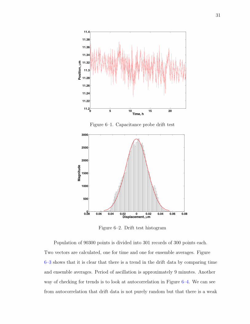
6.2 Drift Test

To establish the performance envelope of the capacitance probe measurements

a drift test is carried out over a period of over 24 hours. For this test a single

capacitance probe is attached to an ”’L’” shaped aluminum bracket. The bracket

both holds the cap probe and also serves as a fixed target. Raw data is presented

in the Figure 6–1 .

Every second 300 samples are taken at 3000Hz and averaged to make a single

data point. Sampling at 3000Hz ensures that harmonic noize from 60Hz building

wiring averages out. This sampling scheme is chosen to match the sampling done

during the actuated tests of ABKC. Standard deviation over the 24 hour period is

0.018µm and range is 0.144µm. A histogram of the data, Figure6–2, shows that the

data is close to normally distributed.

30

31

0 5 10 15 2011.2

11.22

11.24

11.26

11.28

11.3

11.32

11.34

11.36

11.38

11.4

Time, h

Po

siti

on

, µm

Figure 6–1. Capacitance probe drift test

0.08 0.06 0.04 0.02 0 0.02 0.04 0.06 0.080

500

1000

1500

2000

2500

3000

Displacement, µm

Mag

nit

ud

e

Figure 6–2. Drift test histogram

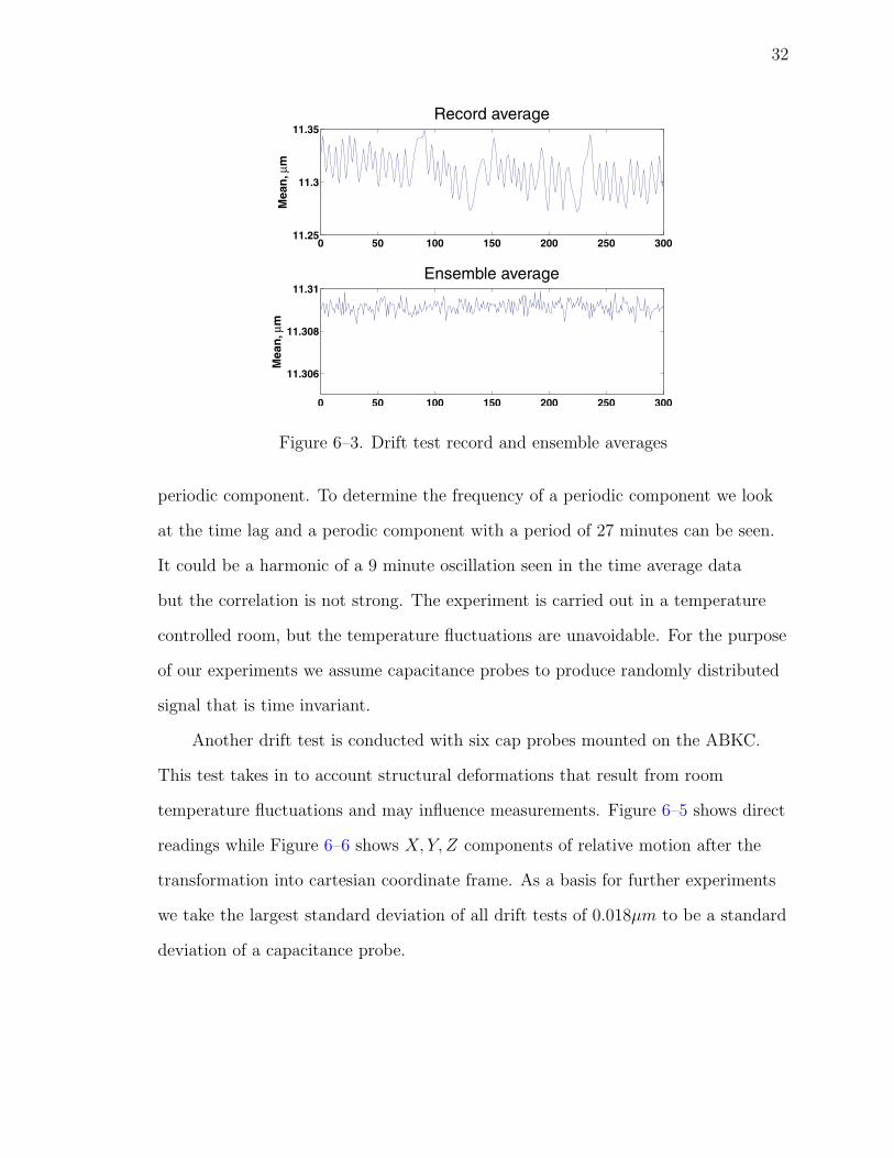
Population of 90300 points is divided into 301 records of 300 points each.

Two vectors are calculated, one for time and one for ensemble averages. Figure

6–3 shows that it is clear that there is a trend in the drift data by comparing time

and ensemble averages. Period of ascillation is approximately 9 minutes. Another

way of checking for trends is to look at autocorrelation in Figure 6–4. We can see

from autocorrelation that drift data is not purely random but that there is a weak

32

0 50 100 150 200 250 30011.25

11.3

11.35

Mea

n, µ

m

Record average

0 50 100 150 200 250 300

11.306

11.308

11.31M

ean

, µm

Ensemble average

Figure 6–3. Drift test record and ensemble averages

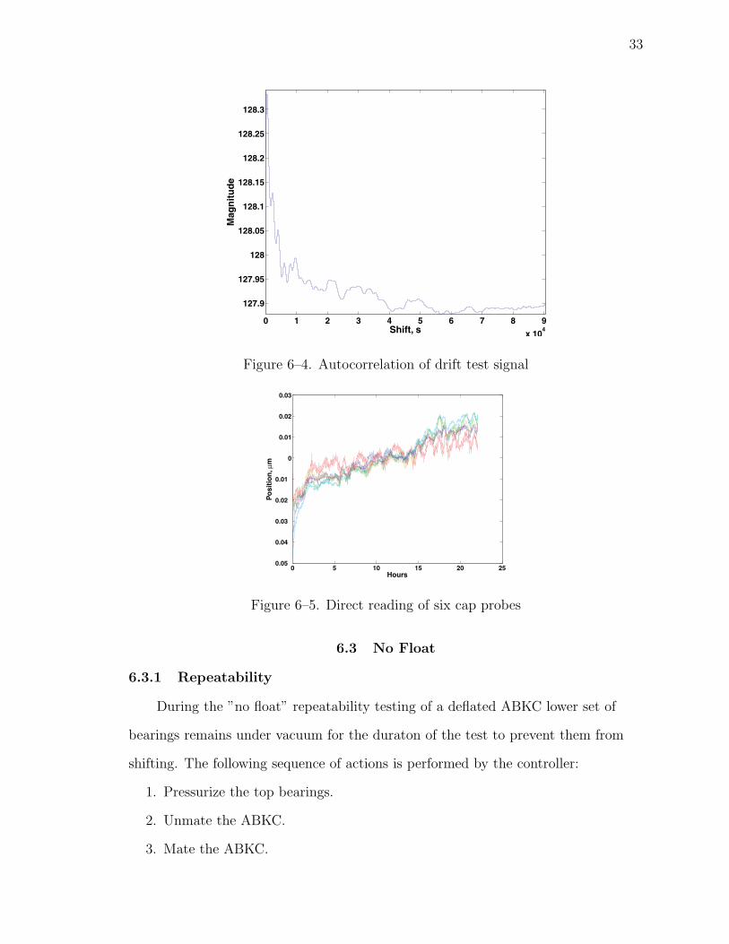
periodic component. To determine the frequency of a periodic component we look

at the time lag and a perodic component with a period of 27 minutes can be seen.

It could be a harmonic of a 9 minute oscillation seen in the time average data

but the correlation is not strong. The experiment is carried out in a temperature

controlled room, but the temperature fluctuations are unavoidable. For the purpose

of our experiments we assume capacitance probes to produce randomly distributed

signal that is time invariant.

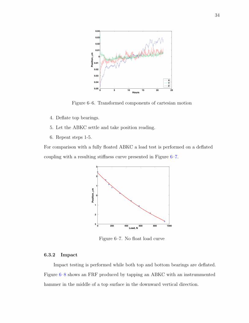
Another drift test is conducted with six cap probes mounted on the ABKC.

This test takes in to account structural deformations that result from room

temperature fluctuations and may influence measurements. Figure 6–5 shows direct

readings while Figure 6–6 shows X, Y, Z components of relative motion after the

transformation into cartesian coordinate frame. As a basis for further experiments

we take the largest standard deviation of all drift tests of 0.018µm to be a standard

deviation of a capacitance probe.

33

0 1 2 3 4 5 6 7 8 9

x 104

127.9

127.95

128

128.05

128.1

128.15

128.2

128.25

128.3

Shift, s

Mag

nit

ud

e

Figure 6–4. Autocorrelation of drift test signal

0 5 10 15 20 250.05

0.04

0.03

0.02

0.01

0

0.01

0.02

0.03

Hours

Po

siti

on

, µm

Figure 6–5. Direct reading of six cap probes

6.3 No Float

6.3.1 Repeatability

During the ”no float” repeatability testing of a deflated ABKC lower set of

bearings remains under vacuum for the duraton of the test to prevent them from

shifting. The following sequence of actions is performed by the controller:

1. Pressurize the top bearings.

2. Unmate the ABKC.

3. Mate the ABKC.

34

0 5 10 15 20 250.05

0.04

0.03

0.02

0.01

0

0.01

0.02

0.03

0.04

HoursP

osi

tio

n, µ

m

XYZ

Figure 6–6. Transformed components of cartesian motion

4. Deflate top bearings.

5. Let the ABKC settle and take position reading.

6. Repeat steps 1-5.

For comparison with a fully floated ABKC a load test is performed on a deflated

coupling with a resulting stiffness curve presented in Figure 6–7.

0 200 400 600 800 10003

2

1

0

1

2

3

Load, N

Po

siti

on

, µm

Figure 6–7. No float load curve

6.3.2 Impact

Impact testing is performed while both top and bottom bearings are deflated.

Figure 6–8 shows an FRF produced by tapping an ABKC with an instrummented

hammer in the middle of a top surface in the downward vertical direction.

35

0 2000 4000 6000 8000 100000

0.005

0.01

0.015

0.02

0.025

0.03

0.035

HzM

agn

itu

de

Figure 6–8. No float FRF

6.4 Half Float

For a ”half float” test the bottom set of bearings is deflated and held under

vacuum to fix them on the base for the duration of the test while top bearings are

held pressurized. Controller carries out the following steps:

1. Unmate the ABKC.

2. Mate the ABKC and allow it to settle.

3. Record position data.

4. Steps 1-3 are repeated.

Figure 6–9 show a portion of data obtained for 100 engagements of ABKC. Strong

dependence of air film thickness on pressure is evident with slope of approximately

1.5µm/bar. Fluctuations in the supply pressure are attributed to the compressor

cycling on and off. It is possible to estimate the repeatability of ABKC if the

pressure were to stay constant. Figures 6–10 and 6–11 show the uncompensated

and compensated repeatability. Standard deviation for uncompensated data is

0.076µm and 0.060µm for compensated data. Due to the geometry of ABKC

angular repeatability is very high, see Figure 6–12.

36

0 20 40 60 80 100-0.35

-0.3

-0.25

-0.2

-0.15

-0.1

-0.05

0

Cycles

Posi

tion,

µm

Cap1Cap2Cap3Cap4Cap5Cap6

6.075

6.11

6.145

6.18

6.215

6.25

Supp

ly P

ress

ure,

bar

Pressure

Figure 6–9. Half float direct probe readings and pressure.

0 200 400 600 800 1000 1200 1400 1600

0.25

0.2

0.15

0.1

0.05

0

0.05

0.1

0.15

0.2

Cycles

Po

siti

on

, µm

xyz

Figure 6–10. Half float uncompensated mating repeatability.

6.5 Full Float

6.5.1 Repeatability

The most interesting results are obtained in the full float tests. In these tests

the ABKC is put through a series of engagement and disengagement cycles with

both top and bottom bearings pressurized. The main interest is in the positional

37

0 200 400 600 800 1000 1200 1400 16000.2

0.15

0.1

0.05

0

0.05

0.1

0.15

0.2

0.25

0.3

Cycles

Po

siti

on

, µm

xyz

Figure 6–11. Half float compensated mating repeatability.

0 200 400 600 800 1000 1200 1400 16005

4

3

2

1

0

1

2

3

4

5x 10

4

Cycles

Ro

tati

on

, µra

d

εx

εy

εz

Figure 6–12. Half float compensated rotational mating repeatability.

repeatability but we are also interested in the frequency response. Over thousands

of cycles the top of the ABKC is removed and then replaced into its position.

Following are the actions the controller performs for each of thousands of cycles.

1. Deflate lower bearings.

2. Apply vacuum to lower bearings.

38

3. Unmate the ABKC.

4. Mate the ABKC and allow it to settle.

5. Pressurise lower bearings to achieve full float.

6. Record position data.

7. Repeat from step 1.

The position of the top with respect to the bottom is recorded and stored. Six

capacitance probes are sampled simultaneously to capture instantaneous relative

displacement.

0 200 400 600 800 1000 1200

0.3

0.25

0.2

0.15

0.1

0.05

0

0.05

0.1

0.15

0.2

Cycles

Po

siti

on

, µm

xyz

Figure 6–13. Full float uncompensated mating repeatability.

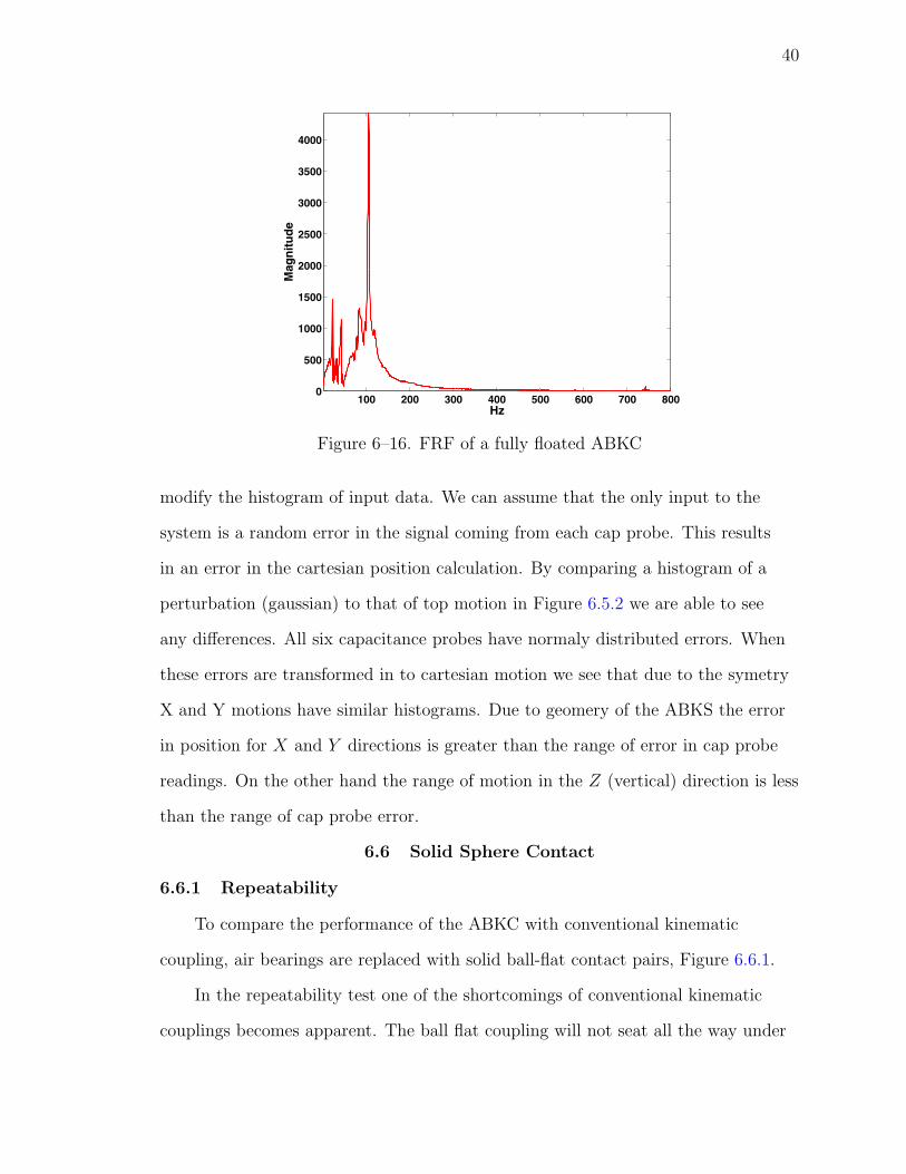
6.5.2 Impact

Impact tests are conducted to capture the natural frequencies of the system.

An FFT of impulse and response is taken and a transfer function is obtained by

dividing response of the system by the input excitation. Capturing data at 20KHz

actually allows us to see structural modes that start at arround 3000Hz, but in this

experiment we are only interested in the rigid body modes in Figure6.5.2.

To evaluate how the uncertainty in capacitance probe measurements

propagates through calculations Montecarlo simmulation is used. Each of six

39

0 200 400 600 800 1000 12000.2

0.1

0

0.1

0.2

0.3

0.4

Cycles

Po

siti

on

, µm

xyz

Figure 6–14. Full float compensated mating repeatability.

0 200 400 600 800 1000 12001

0.8

0.6

0.4

0.2

0

0.2

0.4

0.6

0.8

1x 10

3

Cycles

Ro

tati

on

, µra

d

εx

εy

εz

Figure 6–15. Full float compensated rotational mating repeatability.

cap probe readings is simulated as normaly distributed number with a standard

deviation of .018µm After the capacitance probe readings are transformed in to

a cartisian coordinate system we can look at a histogram of top position. Since

the Jacobian used in coordinate transformation is constant the transformation is

linear. Montecarlo simulation is used only to visualise how transformation will

40

100 200 300 400 500 600 700 8000

500

1000

1500

2000

2500

3000

3500

4000

Hz

Mag

nit

ud

e

Figure 6–16. FRF of a fully floated ABKC

modify the histogram of input data. We can assume that the only input to the

system is a random error in the signal coming from each cap probe. This results

in an error in the cartesian position calculation. By comparing a histogram of a

perturbation (gaussian) to that of top motion in Figure 6.5.2 we are able to see

any differences. All six capacitance probes have normaly distributed errors. When

these errors are transformed in to cartesian motion we see that due to the symetry

X and Y motions have similar histograms. Due to geomery of the ABKS the error

in position for X and Y directions is greater than the range of error in cap probe

readings. On the other hand the range of motion in the Z (vertical) direction is less

than the range of cap probe error.

6.6 Solid Sphere Contact

6.6.1 Repeatability

To compare the performance of the ABKC with conventional kinematic

coupling, air bearings are replaced with solid ball-flat contact pairs, Figure 6.6.1.

In the repeatability test one of the shortcomings of conventional kinematic

couplings becomes apparent. The ball flat coupling will not seat all the way under

41

-0.08 -0.06 -0.04 -0.02 0 0.02 0.04 0.06 0.080

10

20

30

40Input error

Error, µm

-0.08 -0.06 -0.04 -0.02 0 0.02 0.04 0.06 0.080

10

20

30

40X direction error

Error, µm

-0.08 -0.06 -0.04 -0.02 0 0.02 0.04 0.06 0.080

10

20

30

40Z direction error

Error, µm

Figure 6–17. Transformation histograms

Figure 6–18. ABKC converted to ball flat configuration

its own weight due to the frictional forces that arise at the contact points. ABKC

does not have this problem. Figure 6.6.1 illustrates how during automated testing

coupling is unable to come to the equilibrium. Manual setting is required to seat

the coupling.

6.6.2 Impact

Impact testing of solid contact kinematic couping is conducted following the

same procedure as for a fully floated ABKC. Figure 6.6.2 shows an FRF for a

vertical impact.

42

Figure 6–19. Stiction resulting in inability of conventional coupling to mate.

500 1000 1500 2000 2500 3000 3500 4000 4500 50000

10

20

30

40

50

60

Hz

Mag

nit

ud

e

Figure 6–20. Ball flat contact FRF.

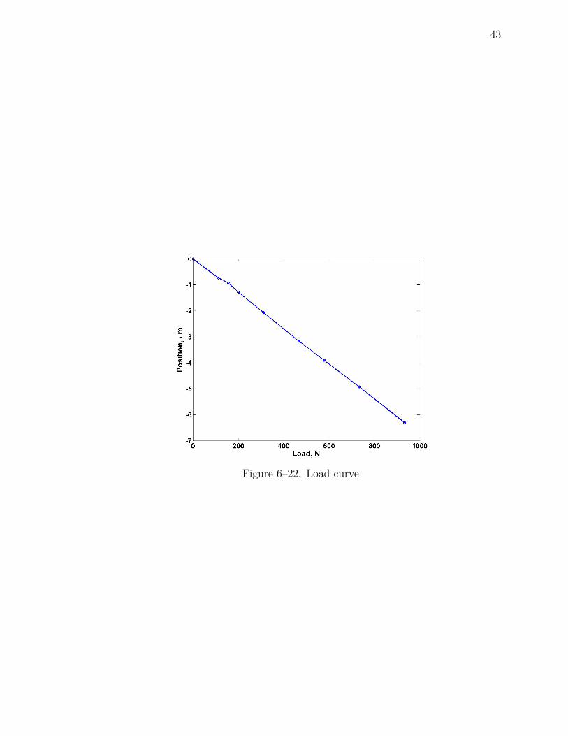
The load capacity of solid contact coupling is tested by placing weights on it

up to a total load of 115 kg as shown in Figure6.6.2. Figure 6.6.2 shows the vertical

displacement of the platform as a function of applied load.

Figure 6–21. Load testing of ABKC

43

Figure 6–22. Load curve

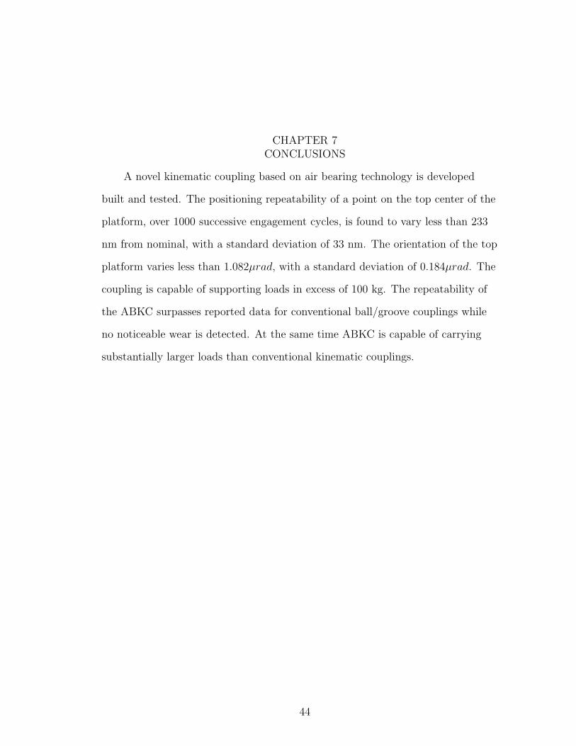
CHAPTER 7CONCLUSIONS

A novel kinematic coupling based on air bearing technology is developed

built and tested. The positioning repeatability of a point on the top center of the

platform, over 1000 successive engagement cycles, is found to vary less than 233

nm from nominal, with a standard deviation of 33 nm. The orientation of the top

platform varies less than 1.082µrad, with a standard deviation of 0.184µrad. The

coupling is capable of supporting loads in excess of 100 kg. The repeatability of

the ABKC surpasses reported data for conventional ball/groove couplings while

no noticeable wear is detected. At the same time ABKC is capable of carrying

substantially larger loads than conventional kinematic couplings.

44

COMPONENT DRAWINGS

Base Drawing

Top Drawing

Damper Drawing

Air Bearing Drawing

Capacitance Probe Holder Drawing

45

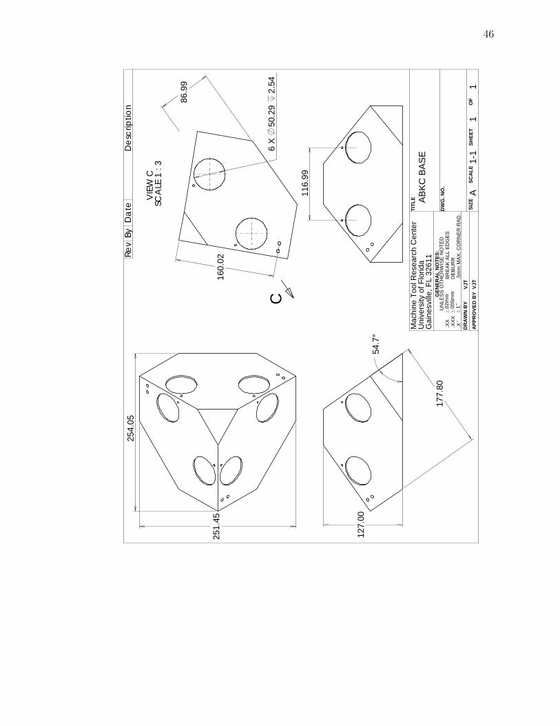
46

54.7

°

127.

00

177.

80

C11

6.99

251.

45

254.

05

6 X

50.2

9 2.

54

160.

02

86.9

9

VIE

W C

SC

ALE

1 :

3

Mac

hine

Too

l Res

earc

h C

ente

rU

nive

rsity

of F

lorid

aG

aine

sville

, FL

3261

1

TITL

E

DW

G. N

O.

SIZE

SCA

LESH

EET

OF

AB

KC

BA

SE

11

1-1

GEN

ERA

L N

OTE

S:U

NLE

SS

OTH

ER

WIS

E N

OTE

D.X

X.X

XX

.X

.02m

m.0

05m

m.1

BRE

AK

ALL

ED

GE

SD

EB

UR

R.5

mm

MA

X. C

OR

NE

R R

AD

.

Rev

ByD

escr

iptio

nD

ate

DR

AW

N B

YA

PPR

OVE

D B

YVJ

TVJ

TA

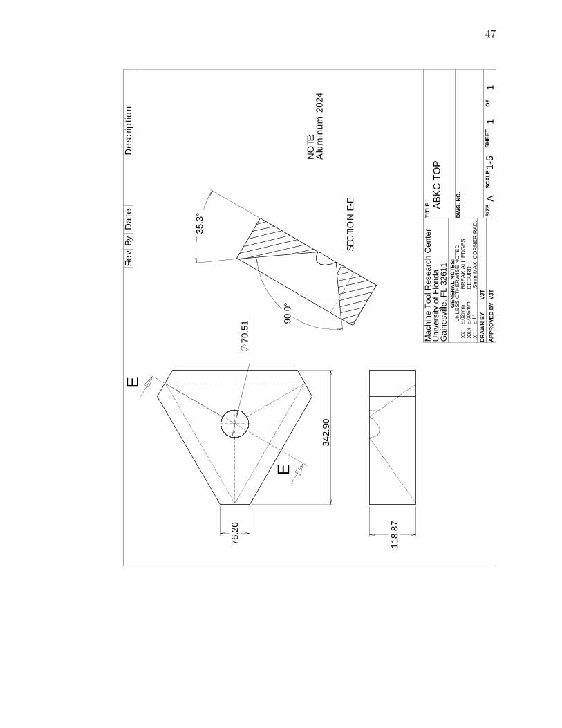
47

70.5

176

.20

342.

90

E

E

118.

87

35.3

°

90.0

°

SEC

TION

E-E

NO

TE:

Alu

min

um 2

024

Mac

hine

Too

l Res

earc

h C

ente

rU

nive

rsity

of F

lorid

aG

aine

sville

, FL

3261

1

TITL

E

DW

G. N

O.

SIZE

SCA

LESH

EET

OF

AB

KC

TO

P

11

1-5

GEN

ERA

L N

OTE

S:U

NLE

SS

OTH

ER

WIS

E N

OTE

D.X

X.X

XX

.X

.02m

m.0

05m

m.1

BR

EA

K A

LL E

DG

ES

DEB

UR

R.5

mm

MAX

. CO

RN

ER R

AD.

Rev

ByD

escr

iptio

nD

ate

DR

AW

N B

YA

PPR

OVE

D B

YVJ

TVJ

TA

48

R25.

15 2

PLA

CES

R32.

77 2

PLA

CES

116.

99

38.1

0

50° 2

PLA

CES

70° 2

PLA

CES

R76.

20 2

PLA

CES

3.18 NO

TE:

2024

alu

min

um

Mac

hine

Too

l Res

earc

h C

ente

rU

nive

rsity

of F

lorid

aG

aine

sville

, FL

3261

1

TITL

E

DW

G. N

O.

SIZE

SCA

LESH

EET

OF

AB

KC

DA

MP

ER

11

1-1

GEN

ERA

L N

OTE

S:U

NLE

SS

OTH

ER

WIS

E N

OTE

D.X

X.X

XX

.X

.02m

m.0

05m

m.1

BRE

AK

ALL

ED

GE

SD

EB

UR

R.5

mm

MA

X. C

OR

NE

R R

AD

.

Rev

ByD

escr

iptio

nD

ate

DR

AW

N B

YA

PPR

OVE

D B

YVJ

TVJ

TA

49

32.9

0

Con

vex

50m

m le

ns

Gla

ss p

late

Con

cave

air

bea

ring

Pla

nar a

ir be

arin

gEp

oxy

Air

film

Air

film

51.3

0

49.9

9M

achi

ne T

ool R

esea

rch

Cen

ter

Uni

vers

ity o

f Flo

rida

Gai

nesv

ille, F

L 32

611

TITL

E

DW

G. N

O.

SIZE

SCA

LESH

EET

OF

AB

KC

AIR

BE

AR

ING

STA

CK

11

1-1

GEN

ERA

L N

OTE

S:U

NLE

SS

OTH

ER

WIS

E N

OTE

D.X

X.X

XX

.X

.02m

m.0

05m

m.1

BR

EA

K A

LL E

DG

ES

DEB

UR

R.5

mm

MAX

. CO

RN

ER R

AD.

Rev

ByD

escr

iptio

nD

ate

DR

AW

N B

YA

PPR

OVE

D B

YVJ

TVJ

TA

50

48.2

6

33.0212.706.99

12.7

030

.48

43.1

8

6.35

6.35

9.53

12.65

6.32

48.2

6

4.04

8.26

4.04

9.53

25.4

0

6.32

Mac

hine

Too

l Res

earc

h C

ente

rU

nive

rsity

of F

lorid

aG

aine

sville

, FL

3261

1

TITL

E

DW

G. N

O.

SIZE

SCA

LESH

EET

OF

AB

KC

CA

P P

RO

BE

HO

LDE

R

11

1-1

GEN

ERA

L N

OTE

S:U

NLE

SS

OTH

ER

WIS

E N

OTE

D.X

X.X

XX

.X

.02m

m.0

05m

m.1

BRE

AK

ALL

ED

GE

SD

EB

UR

R.5

mm

MA

X. C

OR

NE

R R

AD

.

Rev

ByD

escr

iptio

nD

ate

DR

AW

N B

YA

PPR

OVE

D B

YVJ

TVJ

TA

REFERENCES

[1] Schouten, Rosielle, P. Schellekens, “Design of a kinematic coupling forprecision applications” in Precision Engineering 1997;20;46-52.

[2] C. Araque, C. K. Harper, P. Petri, “Low cost kinematic couplings” 2.75-Precision Machine Design Fall 2001 Class Report, Massachusetts Institute ofTechnology, Cambridge, MA, USA

[3] M. L. Culpepper, “Design of quasi-kinematic couplings” in PrecisionEngineering 2004;28;338-357.

[4] M. L. Culpepper, M. Kartik, C. DiBiasio, “Design of integrated eccentricmechanisms and exact constraint fixtures for micron-level repeatability andaccuracy” in Precision Engineering 2005;29;65-80.

[5] L. C. Hale and A. H. Slocum, “Optimal design techniques for kinematiccouplings” in Precision Engineering 2001;25;114-127.

[6] J. -S. Plante, J. Vorgan, T. El-Aguizy, A. H. Slocum, “A design modelfor circular porous air bearings using the 1D generalized flow method” inPrecision Engineering 2005;29;336-346.

[7] P. Schmiechen, A. H. Slocum, “Analysis of kinematic systems: a generalizedapproach.” in Precision Engineering,1996;19;11-18.

[8] A. H. Slocum, “Design of three-groove kinematic couplings” in PrecisionEngineering1992;14;67-73.

[9] A. H. Slocum, A. Donmez, “Kinematic couplings for precision fixturing - Part1: Formulation of design parameters” in Precision Engineering 1988;10;85-91.

[10] A. H. Slocum, A. Donmez, “Kinematic couplings for precision fixturing - Part2: Experimental determination of repeatability and stiffness” in PrecisionEngineering 1988;10;115-122.

[11] R. R. Vallance, C. J. Vogan, A. H. Slocum, “Precisely positioning pallets inmulti-station assembly system” in Precision Engineering 2004;28;218-231.

[12] M. Barraja, R. R. Vallance, “Tolerancing kinematic couplings“ in PrecisionEngineering 2005;29;101-112.

51

52

[13] M.J. Van Doren, “Precision machine design for the semiconductor industry”,Doctoral Thesis, Massachusetts Institute of Technology, Cambridge, MA,USA, May 1995.

BIOGRAPHICAL SKETCH

Vadim Tymianski was born in Russia at the time when it was still a part of

Soviet Union. After accompanying his parents for the move to the United States

in 1992 he attended the University of Florida and graduated in 2001 with BSME.

After working as a design engineer, thirst for knowledge brought him back to UF in

a pursuit of a master’s degree.

Vadim’s future plans include conducting doctoral research at Clemson

University and furthering his consulting practice of Product and Instrument

Design LLC.

53