air force institute of technology - defense ...€œtemple-ism” comments. press-on, sir. second, i...

EVALUATING THE CORRELATION CHARACTERISTICS

OF ARBITRARY AM AND FM RADIO SIGNALS

FOR THE PURPOSE OF NAVIGATION

THESIS

Bryan S. Kim, Second Lieutenant, USAF

AFIT/GE/ENG/06-28

DEPARTMENT OF THE AIR FORCEAIR UNIVERSITY

AIR FORCE INSTITUTE OF TECHNOLOGY

Wright-Patterson Air Force Base, Ohio

APPROVED FOR PUBLIC RELEASE; DISTRIBUTION UNLIMITED.

The views expressed in this thesis are those of the author and do not reflect theofficial policy or position of the United States Air Force, Department of Defense, orU.S. Government.

AFIT/GE/ENG/06-28




THESIS

Presented to the Faculty

Department of Electrical and Computer Engineering

Graduate School of Engineering and Management

Air Force Institute of Technology

Air University

Air Education and Training Command

In Partial Fulfillment of the Requirements for the

Degree of Master of Science in Electrical Engineering

Bryan S. Kim, B.S.E.E.

Second Lieutenant, USAF

March 2006

APPROVED FOR PUBLIC RELEASE; DISTRIBUTION UNLIMITED.

AFIT/GE/ENG/06-28




Bryan S. Kim, B.S.E.E.

Second Lieutenant, USAF

Approved:

/signed/ March 2006

Dr. Michael A. Temple (Chairman) date

/signed/ March 2006

Dr. John F. Raquet (Member) date

/signed/ March 2006

Maj. Todd B. Hale (Member) date

AFIT/GE/ENG/06-28

Abstract

The Global Positioning System (GPS) provides position estimates on Earth at

anytime, anywhere and in any weather. However, GPS requires an unobstructed

path to satellite signals. As such, GPS performance generally degrades or becomes

non-existent in environments such as large urban areas. This research investigates

and analyzes the correlation characteristics of arbitrary AM and FM radio signals for

the purpose of navigation. The primary objective of this research is to determine if

there is any potential for using AM and FM radio signals in a TDOA-type navigation

system. In support of this objective, two correlation receiver methods are considered

with a goal of producing autocorrelation peaks between the received signals of the

reference and target receivers. With successful results, hopefully future work can be

done with these correlation methods and TDOA navigation techniques.

By using a reference signal with known characteristics (i.e., 31-Gold coded wave-

form), the integrity of the designed system model is validated by comparing simulated

and theoretical results. Once the model performs as desired, the AM and FM radio

signals are used as inputs. Simulations are conducted with different combinations of

correlation methods (‘fixed’ or ‘varying’), modulation types (AM or FM), and signal

types (song or voice). Excluding reference signal validation results, there are eight

different variations available for determining whether or not AM and FM radio signals

have correlation characteristics useful for the purpose of navigation.

Out of the eight different variations considered, only two provided promising

results for the purpose of navigation. Both the FM voice and FM song signals exhibit

distinct autocorrelation peaks (i.e., 5.0 dB peak-to-sidelobe ratios) using the ‘fixed’

reference correlation method. However, results for both FM signal types revealed

limited potential for navigation when using the ‘varying’ reference correlation method.

All the AM signals considered yielded relatively limited potential for navigation using

either correlation method.

iv

Acknowledgements

Thank you. I want to extend my thanks to everyone who has supported me

and my efforts during this research. Many of you will go unnamed individually, but

your support has been instrumental in the completion of this thesis and is far from

unappreciated.

First, I would like to thank my thesis advisor, Dr. Temple. His insights, guid-

ance and most importantly, his positive attitude throughout the whole process was

vital for my success. I, as many of his other students, will always remember his many

“Temple-ism” comments. Press-on, sir.

Second, I certainly cannot exclude my fellow students, especially my roommates:

Dex, Matt, and Paul. Your friendships inside and outside the classroom has provided

warm memories throughout our 18 month stay. I am privileged to have met each one

of you and hope that our paths may cross in the future.

Finally, I want to express my love and gratitude for my family back home. They

have always encouraged and believed in me. A part of everything I am is, and will

always be, because of you. Sa rang hae yo.

Bryan S. Kim

v

Table of ContentsPage

Abstract . . . . . . . . . . . . . . . . . . . . . . . . . . . . . . . . . . . . . iv

Acknowledgements . . . . . . . . . . . . . . . . . . . . . . . . . . . . . . . v

List of Figures . . . . . . . . . . . . . . . . . . . . . . . . . . . . . . . . . viii

List of Tables . . . . . . . . . . . . . . . . . . . . . . . . . . . . . . . . . . xi

List of Symbols . . . . . . . . . . . . . . . . . . . . . . . . . . . . . . . . . xii

List of Abbreviations . . . . . . . . . . . . . . . . . . . . . . . . . . . . . . xiii

I. Introduction . . . . . . . . . . . . . . . . . . . . . . . . . . . . . 11.1 Motivation . . . . . . . . . . . . . . . . . . . . . . . . . 1

1.2 Research Objectives . . . . . . . . . . . . . . . . . . . . 3

1.3 Related Research . . . . . . . . . . . . . . . . . . . . . . 5

1.3.1 Radiolocation - Passive Radiodetermination . . 61.3.2 Radionavigation - Active Radiodetermination . 10

1.4 Thesis Outline . . . . . . . . . . . . . . . . . . . . . . . 13

II. Background . . . . . . . . . . . . . . . . . . . . . . . . . . . . . . 15

2.1 Digital Data Modulation . . . . . . . . . . . . . . . . . . 15

2.2 Autocorrelation . . . . . . . . . . . . . . . . . . . . . . . 17

2.3 Gold Coded, Random Binary Waveform . . . . . . . . . 17

2.3.1 Gold Code Family of Sequences . . . . . . . . . 18

2.3.2 Random Binary Waveform . . . . . . . . . . . . 18

2.3.3 Binary Phase Shift Keying . . . . . . . . . . . . 19

2.3.4 31-Gold Code Signal Construction . . . . . . . . 20

2.4 TDOA Positioning . . . . . . . . . . . . . . . . . . . . . 21

2.5 Summary . . . . . . . . . . . . . . . . . . . . . . . . . . 26

III. Methodology . . . . . . . . . . . . . . . . . . . . . . . . . . . . . 27

3.1 Model Development . . . . . . . . . . . . . . . . . . . . 27

3.1.1 Basic Model . . . . . . . . . . . . . . . . . . . . 273.1.2 Receiver Frontend Model . . . . . . . . . . . . . 28

3.2 Signal Types . . . . . . . . . . . . . . . . . . . . . . . . 31

3.2.1 31-Gold Coded Random Binary Waveform . . . 31

3.2.2 AM and FM Radio Waveforms . . . . . . . . . 32

vi

3 Correlator Development . . . . . . . . . . . . . . . . . . 37

3.3.1 Correlation A: “Varying” Reference Correlation 37

3.3.2 Correlation B: “Fixed” Reference Correlation . 40

3.4 Definition of Navigation Potential . . . . . . . . . . . . . 41

3.5 Summary . . . . . . . . . . . . . . . . . . . . . . . . . . 42

IV. Simulation Results and Analysis . . . . . . . . . . . . . . . . . . 43

4.1 Model Verification . . . . . . . . . . . . . . . . . . . . . 43

4.1.1 Frontend Model Results and Analysis . . . . . . 43

4.1.2 Correlation Methods - Varying Sample Delay Nd 46

4.1.3 Correlation Methods - Varying Correlation Win-dow Size Nw . . . . . . . . . . . . . . . . . . . . 52

4.2 AM Radio Signal . . . . . . . . . . . . . . . . . . . . . . 55

4.2.1 AM Song Signal Results and Analysis . . . . . . 56

4.2.2 AM Voice Signal Results and Analysis . . . . . 61

4.3 FM Radio Signal . . . . . . . . . . . . . . . . . . . . . . 66

4.3.1 FM Song Signal Results and Analysis . . . . . . 66

4.3.2 FM Voice Signal Results and Analysis . . . . . 72

4.4 Summary . . . . . . . . . . . . . . . . . . . . . . . . . . 77

V. Conclusions and Recommendations . . . . . . . . . . . . . . . . . 785.1 Summary of Results . . . . . . . . . . . . . . . . . . . . 78

5.1.1 Correlation Receiver Model Results . . . . . . . 785.1.2 Correlation Peak Identifiability of AM Radio . . 80

5.1.3 Correlation Peak Identifiability of FM Radio . . 81

5.2 Future Work . . . . . . . . . . . . . . . . . . . . . . . . 83

Appendix A. MATLAB Code for Correlation Methods . . . . . . . . . 85

Bibliography . . . . . . . . . . . . . . . . . . . . . . . . . . . . . . . . . . 87

vii

List of Figures

Figure Page

1.1. AOA Position Estimate Technique . . . . . . . . . . . . . . . . 7

1.2. Trilateration . . . . . . . . . . . . . . . . . . . . . . . . . . . . 9

1.3. GEE Navigation System . . . . . . . . . . . . . . . . . . . . . . 12

2.1. Fourier Transform of Cosine . . . . . . . . . . . . . . . . . . . . 16

2.2. 31-Gold Code Sequence . . . . . . . . . . . . . . . . . . . . . . 18

2.3. BPSK Transmitter Model . . . . . . . . . . . . . . . . . . . . . 21

2.4. Transmitted Waveform PSD (Continuous) . . . . . . . . . . . . 22

2.5. TDOA Range Estimates . . . . . . . . . . . . . . . . . . . . . . 23

2.6. TDOA System with Three Signal Sources . . . . . . . . . . . . 23

3.1. Basic Transmit-Receive Model . . . . . . . . . . . . . . . . . . 27

3.2. Major Receiver Components . . . . . . . . . . . . . . . . . . . 28

3.3. Receiver Frontend Model . . . . . . . . . . . . . . . . . . . . . 30

3.4. 31-Gold Coded Random Binary Waveform . . . . . . . . . . . . 33

3.5. Baseband Song Signal . . . . . . . . . . . . . . . . . . . . . . . 33

3.6. Baseband Voice Signal . . . . . . . . . . . . . . . . . . . . . . . 34

3.7. AM Song Signal . . . . . . . . . . . . . . . . . . . . . . . . . . 34

3.8. AM Voice Signal . . . . . . . . . . . . . . . . . . . . . . . . . . 35

3.9. FM Song Signal . . . . . . . . . . . . . . . . . . . . . . . . . . 36

3.10. FM Voice Signal . . . . . . . . . . . . . . . . . . . . . . . . . . 37

3.11. Correlation A - “Varying” Reference Correlation . . . . . . . . 38

3.12. Example of Correlation A - “Varying” Reference Correlation . 39

3.13. Correlation B - “Fixed” Reference Correlation . . . . . . . . . 39

3.14. Example of Correlation B - “Fixed” Reference Correlation . . . 40

4.1. Frontend Process - RF Filter Results . . . . . . . . . . . . . . . 44

4.2. Frontend Process - Downconversion and BB Filter Results . . . 44

viii

Figure Page

4.3. Correlation-A output for RBW signal . . . . . . . . . . . . . . 47

4.4. Correlation-A outputs for Nd equal 1 and 500 . . . . . . . . . . 48

4.5. Magnitude of Correlation-A output (dB scale) for RBW signal 48

4.6. Magnitude of Correlation-A outputs (dB scale) for Nd equal 1

and 500 . . . . . . . . . . . . . . . . . . . . . . . . . . . . . . . 49

4.7. Correlation-B output for RBW signal . . . . . . . . . . . . . . 49

4.8. Correlation-B outputs for 100th and 749th reference window . . 50

4.9. Magnitude of Correlation-B output (dB scale) for RBW signal 50

4.10. Magnitude of Correlation-B outputs (dB scale) for 100th and

749th reference window . . . . . . . . . . . . . . . . . . . . . . 51

4.11. Correlation-A output for RBW signal when varying Nw . . . . 53

4.12. Correlation-B output for RBW signal when varying Nw . . . . 54

4.13. Conditioned AM song signal . . . . . . . . . . . . . . . . . . . 56

4.14. Correlation-A output for AM song signal . . . . . . . . . . . . 57

4.15. Magnitude of Correlation-A output (dB scale) for AM song signal 57

4.16. Magnitude of Correlation-A outputs (dB scale) for 1st and 500th

reference window . . . . . . . . . . . . . . . . . . . . . . . . . . 58

4.17. Correlation-B output for AM song signal . . . . . . . . . . . . 59

4.18. Magnitude of Correlation-B output (dB scale) for AM song signal 59

4.19. Magnitude of Correlation-B outputs (dB scale) for 9th and 1635th


4.20. Conditioned AM voice signal . . . . . . . . . . . . . . . . . . . 61

4.21. Correlation-A output for AM voice signal . . . . . . . . . . . . 62

4.22. Magnitude of Correlation-A output (dB scale) for AM voice signal 63



4.24. Correlation-B output for AM voice signal . . . . . . . . . . . . 64

4.25. Magnitude of Correlation-B output (dB scale) for AM voice signal 65

ix

Figure Page



4.27. Conditioned FM song signal . . . . . . . . . . . . . . . . . . . 67

4.28. Correlation-A output for FM song signal . . . . . . . . . . . . . 68

4.29. Magnitude of Correlation-A output (dB scale) for FM song signal 68



4.31. Correlation-B output for FM song signal . . . . . . . . . . . . . 70

4.32. Magnitude of Correlation-B output (dB scale) for FM song signal 70



4.34. Conditioned FM voice signal . . . . . . . . . . . . . . . . . . . 72

4.35. Correlation-A output for FM voice signal . . . . . . . . . . . . 73

4.36. Magnitude of Correlation-A output (dB scale) for FM voice signal 73



4.38. Correlation-B output for FM voice signal . . . . . . . . . . . . 75

4.39. Magnitude of Correlation-B output (dB scale) for FM voice signal 76


1846th reference window . . . . . . . . . . . . . . . . . . . . . 76

x

List of Tables

Table Page

2.1. Autocorrelation Properties for a Real-Valued Signal . . . . . . 17

3.1. Statistics of 31-Gold Spreading Code . . . . . . . . . . . . . . . 32

4.1. Bandwidth for Frontend Process Filters . . . . . . . . . . . . . 45

4.2. Nw and ∆w Values of Correlation-A . . . . . . . . . . . . . . . 54

4.3. Nw and ∆w Values of Correlation-B . . . . . . . . . . . . . . . 55

xi

List of Symbols

Symbol Page

Rx(τ) Autocorrelation function . . . . . . . . . . . . . . . . . . . 17

Rc Chip rate . . . . . . . . . . . . . . . . . . . . . . . . . . . 21

RD Bit/Data rate . . . . . . . . . . . . . . . . . . . . . . . . . 21

st(t) Transmitted signal . . . . . . . . . . . . . . . . . . . . . . 27

sr(t) Signal acquired at receiver’s frontend . . . . . . . . . . . . 27

Cd Channel signal delay . . . . . . . . . . . . . . . . . . . . . 28

n(t) Additive White Gaussian Noise (AWGN) signal . . . . . . 28

HRF 2nd-Order Butterworth RF filter . . . . . . . . . . . . . . 28

sRF Output signal to HRF . . . . . . . . . . . . . . . . . . . . 28

sLO Local Oscillator signal . . . . . . . . . . . . . . . . . . . . 29

xI(t) In-phase mixed signal . . . . . . . . . . . . . . . . . . . . 29

xQ(t) Quadrature mixed signal . . . . . . . . . . . . . . . . . . . 29

HBB 2nd-Order Butterworth BB filter . . . . . . . . . . . . . . 29

C(t) Spreading code waveform . . . . . . . . . . . . . . . . . . 31

d(t) Information data stream . . . . . . . . . . . . . . . . . . . 31

Nd Number of samples to delay signal . . . . . . . . . . . . . 38

Nw Number of samples in a correlation window . . . . . . . . 38

∆w Number of samples shifted between correlation iterations . 38

Ni Total number of signal samples . . . . . . . . . . . . . . . 38

xii

List of Abbreviations

Abbreviation Page

AM Amplitude Modulated . . . . . . . . . . . . . . . . . . . . 1

FM Frequency Modulated . . . . . . . . . . . . . . . . . . . . 1

GPS Global Positioning System . . . . . . . . . . . . . . . . . . 1

SOP Signals of Opportunity . . . . . . . . . . . . . . . . . . . . 1

INS Inertial Navigation System . . . . . . . . . . . . . . . . . . 2

NTSC National Television System Committee . . . . . . . . . . . 2

CDMA Code Division Multiple Access . . . . . . . . . . . . . . . 2

CPI Correlation Peak Identifiability . . . . . . . . . . . . . . . 3

TDOA Time Difference of Arrival . . . . . . . . . . . . . . . . . . 3

SOI Signal of Interest . . . . . . . . . . . . . . . . . . . . . . . 4

AOA Angle of Arrival . . . . . . . . . . . . . . . . . . . . . . . 6

TOA Time of Arrival . . . . . . . . . . . . . . . . . . . . . . . . 6

RDF Radio Direction Finder . . . . . . . . . . . . . . . . . . . . 10

VOR VHF Omnidirectional Range . . . . . . . . . . . . . . . . 11

LORAN Long Range Navigation . . . . . . . . . . . . . . . . . . . 13

RF Radio Frequency . . . . . . . . . . . . . . . . . . . . . . . 15

IF Intermediate Frequency . . . . . . . . . . . . . . . . . . . 15

RBW Random Binary Waveform . . . . . . . . . . . . . . . . . . 18

BPSK Binary Phase Shift Keying . . . . . . . . . . . . . . . . . . 18

PRBW Pseudo Random Binary Waveform . . . . . . . . . . . . . 18

PSK Phase Shift Keying . . . . . . . . . . . . . . . . . . . . . . 19

AWGN Additive White Gaussian Noise . . . . . . . . . . . . . . . 28

LO Local Oscillator . . . . . . . . . . . . . . . . . . . . . . . . 29

I&Q In-phase&Quadrature . . . . . . . . . . . . . . . . . . . . 29

BB Baseband . . . . . . . . . . . . . . . . . . . . . . . . . . . 29

xiii

Abbreviation Page

FIR Finite Impulse Response . . . . . . . . . . . . . . . . . . . 30

IIR Infinite Impulse Response . . . . . . . . . . . . . . . . . . 30

PSD Power Spectral Density . . . . . . . . . . . . . . . . . . . 32

USRP Universal Software Radio Peripheral . . . . . . . . . . . . 83

xiv




I. Introduction

This chapter provides the reason and goals for researching the correlation char-

acteristics of arbitrary Amplitude Modulated (AM) and Frequency Modulated

(FM) radio signals for the purpose of navigation. Section 1.1 explains the motivation

and relevancy of this research. Section 1.2 discusses the two main goals set for this

research model. Section 1.3 gives an overview of previous research done in related

fields. An outline of the thesis is given in Section 1.4.

1.1 Motivation

The Global Positioning System (GPS) provides position estimates on the Earth

at anytime, anywhere and in any weather. However, to provide robust position-

ing performance, GPS requires an unobstructed path to satellite signals. As such,

GPS performance generally degrades or becomes non-existent in environments such

as under dense vegetation, indoors, or in larger urban areas. So the use of non-GPS

waveforms, commonly referred to as “signals of opportunity (SOP)” and including

such signals as television broadcasts, cellular communications, AM radio, and FM

radio, are being considered as alternatives for position estimation. The SOPs were

specifically designed for purposes other than position estimation and are being studied

to characterize navigation potential for non-GPS waveforms in urban areas [21]. This

research investigates the correlation characteristics of arbitrary AM and FM radio

signals for the purpose of navigation.

There is a great need for the military to develop non-GPS precision navigation

technologies in order to be able to operate in environments where GPS is unavailable

1

[13]. Additional systems are needed to assist in the weaknesses of GPS or, in the worse-

case unlikely scenario, backup and assume the responsibilities of GPS. The GPS is

only a single system and a system failure could occur unexpectedly. There are other

systems such as the Inertial Navigation System (INS) that can provide navigation

capabilities, but these capabilities are only short-term and are not absolute position

solutions [5]. So alternative systems need to be developed to backup or compliment

the current GPS.

The aforementioned SOPs which are available as potential navigation signals in-

clude television broadcasts, cellular communications, AM radio, and FM radio. Each

SOP has specific properties and characteristics that could be exploited for navigation

however, AM and FM radio was selected for the following reasons.

The navigation potential of television broadcasting signals, or more specifically

the National Television System Committee (NTSC) television broadcast signal, has

been previously investigated in [5]. Follow-on work on the NTSC television broadcast

could have been selected as the topic of this thesis, but there is interest in determining

navigation potential for different waveforms.

Cellular communication waveforms, such as used for the Code Division Multiple

Access (CDMA) IS-95 Digital Cellular Network, possess particular characteristics that

make them potential candidates for navigation. The IS-95 Digital Cellular Network

uses many signals and channels. One of the channels is called the pilot channel and

this channel has a coded signal that allows the users to synchronize within the system.

For every user or mobile on the system, the CDMA system assigns a specific digital

code. These codes are so specific that multiple users can transmit simultaneously on

the same frequency without interfering with each other [17]. The transmitted signal

is a 32,767 bit pseudo-random “short” code that repeats 37.5 times per second [16].

Since this code is known along with other signal properties, correlation techniques

can be used to estimate the time of signal reception. Position estimation can then be

determined based on the time estimates of 4 or more independent signals. However,

2

the CDMA IS-95 network is an impractical alternative for GPS because it requires

time-synchronization from GPS [5].

There are three reasons why the AM and FM radio signals were selected as the

SOP of interest for this research. First, AM and FM radio signals are transmitted

with more power and at a closer range than GPS signals. Approximately 50 watts

of power are used to transmit signals from GPS satellites [14]. Typical AM and

FM radio stations operate at transmit power levels up to 50 kilowatts [2]. Radio

signals being transmitted at higher power correspond to stronger signals indoors and

in urban areas. GPS signals typically cannot be received in these environments, but

radio signals can be received. Second, the radio transmitters are stationary land-

based locations whereas GPS has up to 32 orbiting satellites [14]. Stationary land-

based locations not only allow for less complex navigation computations but more

importantly, this eliminates some of the errors introduced by space-vehicle position

and atmospheric effects [5]. Finally, radio signals are broadcasted at frequencies

between 530 kHz to 1710 kHz for AM radio and between 87 MHz to 108MHz for FM

radio. The carrier frequencies of GPS signals are 1227.6 MHz and 1575.42 MHz [14].

The number of different frequencies available for AM and FM radio signals improves

system operability by giving the potential to avoid interference at a signal frequency

[5].

1.2 Research Objectives

The main concept for this research is derived from the concepts developed in [5,7]

for the NTSC television signal. The methodology and results between this thesis and

the work done in [5,7] are quite different. The research documented in [5,7] dealt with

the navigation potential of the NTSC broadcast signal, while this research investigates

the Correlation Peak Identifiability (CPI) of arbitrary AM and FM radio signals. The

promising navigation potential of the NTSC broadcast signal has increased curiosity

regarding whether or not AM and/or FM radio signals have navigation potential using

similar time-difference-of-arrival (TDOA) navigation methods. The main difference

3

between this research and [5, 7] is that [5, 7] already assumed the user knew which

correlation peak was being tracked so that ‘navigation potential’ could be defined

as the accuracy with which the user could estimate the time difference between a

reference and target receiver. This research will determine how well the user will be

able to distinguish and locate the correct correlation peak, thus the acronym CPI. In

the real world, both the ability to locate the correct correlation peak and the ability

to get accurate estimates of the time delay between the reference and target receivers

are needed for navigation.

The TDOA navigation system is a range-based method of determining position

by measuring the difference in arrival time of a signal between two receivers [31]. Two

receivers, a reference receiver and a target receiver, are used to eliminate the need for

any time synchronization in the signal of interest (SOI). The stationary location of

the reference receiver is already known while the location of the mobile target receiver

is at the point of interest. Since the location of the transmitter (i.e., signal source)

is also known, once the SOI is received at both receivers and time-tagged, the time

difference of how much more or less time the SOI took to get to the target receiver than

the reference receiver can be determined. This time difference can then be converted

to range using the speed of light. These range measurements tell how much closer

or farther the target receiver was from the transmitter than the reference receiver

was from the transmitter. So ultimately, the actual distance between the target

receiver and transmitter can be calculated using TDOA [31]. Position estimation can

then be determined based on the TDOA measurements from 4 or more independent

signal sources. Three independent signal sources are needed for position while one

independent signal source is needed to account for differential receiver clock error. In

a real world application, the calculated range is actually a “pseudorange” meaning a

measurement including range and clock error. Multi-lateration algorithms are then

used on these pseudoranges to determine position estimation and clock errors [14].

These receiver clock errors while small can cause large error in position estimation

and need to be accounted.

4

The CPI of arbitrary AM and FM radio signals for the purpose of navigation

is investigated and analyzed based on the results of correlation functions. So the

first objective of this research is to develop two separate correlation methods that

will hopefully produce desired autocorrelation peaks using the received SOI of the

reference and target receivers. Two approaches are developed to add diversity to the

research. Ideally, the two correlation methods are developed so that any generic signal

can be analyzed as the input signal and not just AM or FM radio signals. Models

for the two correlation methods are developed, analyzed and verified by using a Gold

coded BPSK waveform as the input signal. This waveform was chosen because it

has known characteristics and correlation structure. With known characteristics, a

comparison between the actual results and the theoretical results can be made to

verify the performance of the models.

The primary objective of this research is to determine if there is any potential

for using AM and FM radio signals in a TDOA-type navigation system by determin-

ing CPI. As a first step for assessing CPI, the results of two correlation models are

analyzed when AM and FM radio signals are used as the input signal. The results

from the correlation models will hopefully show some navigation potential so future

work can be done with these correlation methods and TDOA navigation techniques.

1.3 Related Research

There are many related and similar topics on navigation systems already inves-

tigated and presented to the technical community. There is a study called radiodeter-

mination which is “the determination of position, velocity and/or other characteristics

of an object, or the obtaining of information relating to these parameters, by means

of the propagation properties of radio waves [26].” There are two main types of ra-

diodetermination. The first part of this section discusses the typical passive type

of radiodetermination, radio location, while the second part of this section discusses

the usually active type of radiodetermination, radionavigation. Different navigation

systems within each radiodetermination category are also be presented.

5

1.3.1 Radiolocation - Passive Radiodetermination. The passive type of

radiodetermination is radiolocation which is the process of finding an object using

radio waves [27]. The most well known system that uses radiolocation is the radar.

A radar is considered a passive system because it finds the location of an object

rather than actively finding one’s own position. The location of the object can be

determined from the angle at which the signal returns and/or the time it takes to

return. These two techniques are most commonly seen in estimating the position of a

mobile receiver. The angle-of-arrival (AOA) and time-of-arrival (TOA) measurement

techniques are discussed below.

1.3.1.1 Angle of Arrival (AOA). The AOA technique is the method

of using angles between a receiver and transmitters to determine position. AOA

requires, at least, the known location of two signal sources to determine the user’s

position in two dimensions. The user’s position is located at the intersection point of

the angle lines from each signal source. When the receiver locates each signal source,

the individual signal angles are estimated by comparing either the signal amplitude or

carrier-phase at an interferometer (i.e., multiple calibrated antennas) [1]. The signal

amplitude comparison is less complicated than the carrier-phase method but it is

also less accurate. The accuracy of a two antenna phase-comparison interferometer

produces sub-degree angle estimations [22].

The AOA technique can be best seen with the classic example of how a ship

determines its position using the known location of two landmarks (i.e., lighthouses

or stationary buoys) [4]. With the use of a compass and map, the angle between

the ship and two known landmarks can be drawn to show an intersection point.

This intersection point is the position estimation for the two-dimensional case. This

technique obviously has sources of error that degrade the position estimation accuracy.

But the error can be reduced by using a third landmark. Figure 1.1 shows the AOA

technique. Note that the center of the resulting triangle is the position estimation.

6

2 Source Estimate

Source 1 Source 2

Source 3

3 Source Estimate

Figure 1.1: AOA Position Estimate Technique using 2 or 3Angle Measurements [5]

This estimation was determined by assuming all measurements and plots are equally

accurate [5].

This passive navigation technique is a simple concept. AOA does not require

extremely accurate time synchronization and it can easily incorporate any SOP in

determining a location. The biggest downfall, however, is that AOA’s accuracy is very

range dependent. As the distance between the receiver and signal sources becomes

greater, the errors in the direction measurement becomes greater producing larger

position estimate errors [3].

1.3.1.2 Time of Arrival (TOA). The TOA technique is the method

of using propagation time of a signal between a transmitter and receiver to estimate

range. This method does require precise time synchronization between all transmit-

ters. Synchronizing the receiver clock is unnecessary because with all the transmitters

synchronized, the receiver clock error is constant for all transmitters. This receiver

clock error can be accounted for by doing one more additional measurement, allowing

the error to be eliminated from the measurements [5]. So with the receiver knowing

7

the clock error and the times of transmission and arrival, the propagation time can be

determined. And with the propagation times, position estimation can be calculated

with trilateration. Trilateration is using measurements of TOA to estimate location

using the intersection of hyperboloids [29].

1.3.1.3 TOA Application - Trilateration. The simplest of the basic

principles of radio wave propagation is that waveforms travel at the known speed

of light. Therefore, given this speed constant, the transit time of a signal from a

transmitting station can be measured. Then using this transmit time, the distance

between the transmitter and receiver can also be determined [10]. The receiver can

compute its position unambiguously if given distances to three transmitters at known

locations. The estimation of a position based on measurement of distances is referred

to as trilateration. Another way to understand trilateration is to define it as the

method of determining the relative position of objects using the geometry of circles

[29]. This method of trilateration uses the known locations of two or more reference

points, and the measured distance between the subject and each reference points. In

general, at least three reference points are need to accurately and uniquely determine

the relative location of a point on a two dimensional plane using trilateration. Figure

1.2 is an illustration of trilateration in two dimensions. P1, P2 and P3 are the known

locations. With only one circle, the position estimation can be narrowed to anywhere

on the P1 circle. The possible locations are then minimized to two points with the

addition of the P2 circle. Points A and B are the intersection points to the P1

and P2 circles. Adding a third circle eliminates one of the two remaining points

and identifies the true location B. This is an example of needing at least 3 reference

points to accurately and uniquely determine the relative location of a point on a two

dimensional plane using trilateration.

For generalization, the reason that three points are required lies in the geometry

of circles. If the distance of a subject point from some fixed reference point, then that

point could exist anywhere on a circle of that radius from the reference. If it is

8

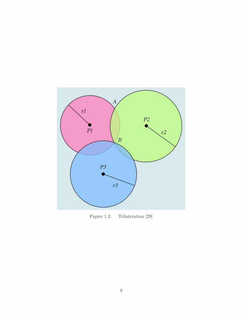
Figure 1.2: Trilateration [29]

9

known that it is also a certain distance from a second reference point, then it also

exists somewhere on a circle of that radius from the second reference point. These

two circles almost always intersect at two points, and the subject could be at either

point. In the case above, these points were A and B. The distance between the

subject and a third reference point introduces a third circle into the diagram, and

all three circles intersect at one point only. The position of the subject is relative to

the three reference points [29]. This basic overview of trilateration assumes that the

subject and the reference points all exist on one plane, implying that there are only

two dimensions involved. For three dimensions, 4 reference points are needed and the

subject point exists on the surface of 3-dimensional spheres instead of 2-dimensional

circles. Two points almost always narrow it down to a circle, and three points to two

points. Apart from those differences, the approach and technique are still the same.

Note that in some real world applications that the minimum number of reference

points may be required to disambiguate the subject’s location. For example, in GPS

if the subject is known to be on the surface of the Earth and the other intersection

point is located in space, the point in space may be disregarded [14]. On the other

hand, the stated number of reference points may not be enough if the geometry is

singular [29].

1.3.2 Radionavigation - Active Radiodetermination. The active type of

radiodetermination is the application of radio frequencies to determine a position

on the Earth [28]. Radionavigation is very similar to radiolocation but rather than

passively finding a distant object, radionavigation actively finds the user’s location.

The earliest radionavigation systems used celestial navigation methods. By using

stars and planets, a person was able to determine his/her location on Earth. However

this method only worked on clear nights. A different navigation method that would

work in all weather and at all time of the day needed to be developed. So the first

radionavigation system was developed, the radio direction finder (RDF). This system

used an directional antenna to tune into a radio station. Since the directional antenna

10

was tuned into broadcasting antenna, the line of reception is also known. A current

location could then be determined by taking two such measurements and plotting

them on a map. Older systems used a hand-rotated loop antenna to find the angle

of the signal. More modern systems use automated motorized directional solenoid to

rapidly take measurements and then calculate the angle using computing software [28].

Not only were commercial AM radio stations used in this technology because of the

long range and high power of AM signals, but strings of low-power radio beacons were

also set up specifically for this system [28].

Other than GPS, there are other radionavigation systems that have been suc-

cessfully implemented in the past, each of which is briefly described below.

1.3.2.1 Lorenz Navigation System. The Lorenz or “Ultrakurzwellen-

Landefunkfeuer” is a radionavigation system that was developed in the 1930s by the

Germans as a night and bad weather landing system [25]. The basic concept of this

system is to place a ‘guiding beam’ near the end of a runway to help navigate and

land aircraft. The guiding beam has two signals broadcasted from highly directional

antennas with each signal beam a few degrees wide. The signals are on the same

frequency and transmitted at slightly different angles so that there is a small overlap

in the middle of the guiding beam. Each signal was selected to emit a dash or

a dot sound. When timed correctly, the dash and dot signals would link together

producing one continuous sound in the overlapped section. Pilots were able to listen

and determine where in the guiding beam they were in and respond accordingly [25].

The pilot’s goal was to find the constant sound and remain on that course until the

runway could be seen visually for safe landing.

1.3.2.2 VHF Omnidirectional Range (VOR). The VHF omnidirec-

tional range (VOR) navigation system is very similar to the Lorenz system but rather

than use sound to navigate, VOR uses two signals that vary in phase to provide more

accurate and reliable measurements. The first ‘master’ signal is transmitted contin-

uously where in comparison, the second ‘highly directional’ signal is transmitted so

11

Figure 1.3: GEE Navigation System [9]

that it varies in phase 3600 times a second faster. These signals are timed so that

the phase varies as the secondary antenna rotates, such that when the antenna is 90

degrees from north, the signal is 90 degrees out of phase from the master [30]. By com-

paring the phase between the two signals, an angle can be determined and displayed

for the pilot. Taking multiple such measurements, the aircraft location estimate can

be made and used for safe landing [30].

1.3.2.3 GEE Navigation System. The GEE or “AMES Type 7000”

navigation system was developed by the British to determine aircraft or ship location

by analyzing the delay times between two sets of signals [9]. Figure 1.3 illustrates

the GEE navigation system. There are three transmitters including one ‘master’ and

two ‘slaves’, ‘A’ and ‘B’. By transmitting precisely timed signals, a user can analyze

12

the signal’s time of arrival from each transmitter to determine relative location. For

example, if signals from two transmitters arrive at the same time, the user must be

equal distances from each signal source. This allows the user to draw a line on the map

for all the positions that are equal distances from the transmitters. Taking similar

measurements with other stations construct other lines, which hopefully lead to an

intersection point [23]. This intersection point is the position estimation.

1.3.2.4 Long Range Navigation (LORAN). The long range naviga-

tion (LORAN) system is a terrestrial navigation system that uses low-frequency ra-

dio transmitters to calculate time intervals between signal sources so that a position

estimate can be determined [24]. LORAN was developed from the basic GEE prin-

ciple and uses a similar master-slave transmitter network. However instead of using

the same one-master/two-slaves arrangement as GEE, LORAN uses one master sta-

tion and four to six slaves stations [24]. The master station broadcasts a series of

short pulses which are received and re-broadcasted by multiple slave stations. The

re-broadcasting by the four to six slave stations creates a chain-effect. Since the

transmitters are synchronized, the time it takes for a radio signal to travel between

transmitter stations and target receiver can be easily measured. With enough mea-

surements, the hyperbolas will intersect providing a final position estimate [24].

1.4 Thesis Outline

Chapter I provided the motivation for researching the navigation potential of

AM and FM radio signals as well as an overview of other related topics. Chapter II

discusses the necessary background needed to understand the major concepts done

in this research including trilateration, TDOA, filtering, autocorrelation, modulation,

random binary waveforms, and the 31-Gold code. Chapter III describes the system

model and parameters used to evaluate the CPI of arbitrary AM and FM radio signals

for the purpose of navigation. Chapter IV presents simulated results and analysis

conducted with the receiver model and two correlation methods developed. Chapter V

13

gives the overall system results and conclusions, followed by recommendations for

further research in using AM and/or FM radio signals in a TDOA algorithm.

14

II. Background

This chapter provides the necessary background for the major topics in this the-

sis. Section 2.1 discusses the basic concepts of digital modulation. Section 2.2

provides the definition and relevant properties of autocorrelation. Section 2.3 explains

the concepts needed to construct the 31-Gold random binary waveform, as used for

a reference signal during code verification and validation. Section 2.4 provides the

overall concept of TDOA.

2.1 Digital Data Modulation

Digital data modulation is a method of converting analog information, such

as song or voice, to binary code for transmission. For baseband modulation, these

waveforms are put onto a carrier wave to enhance transmission efficiency. Without

the carrier modulation, signal transmission would require larger sized antennas. The

antenna’s physical size usually depends on the wavelength λ (λ = speed-of-light c /

frequency f ) and the application. For example, cellular telephone systems typically

have antennas that are λ/4 in size. So without carrier modulation, it would take an

antenna approximately 15 miles long to transmit a f = 3000 Hz baseband signal [18].

But with carrier-wave modulation at a higher frequency, i.e., f = 900 MHz carrier, the

equivalent antenna diameter would be around 8 cm [18]. Therefore, carrier modulation

is an essential step for all radio transmission systems.

Other than transmission efficiency using smaller antennas, carrier modulation

provides additional benefits as well. Modulation is important in this research because

it allows the user to place the SOI in a desired frequency band where designer re-

quirements, such as filtering and amplification, can be easily met. This is the case

where radio-frequency (RF) signals are converted to an intermediate frequency (IF)

in the frontend of a receiver [18]. The following modulation properties are important

for this research.

15

|X(f)|

A/2A/2

f

fo-fo

Figure 2.1: Fourier Transform of Cosine [19]

Equation 2.1 shows the Fourier transform a cosine signal. The Fourier transform

of the left-hand side results in a pair of delta functions located at ±fo and having

one-half the amplitude. Figure 2.1 shows the Fourier transform of (2.1).

A · cos(2πfot) ⇐⇒A

2· {δ(f − fo) + δ(f + fo)} (2.1)

Equation 2.2 shows the Fourier transform relationship for an arbitrary signal

x(t) multiplied by the cosine function (the carrier modulation process). The Fourier

transform of the left-hand side of (2.2) produces in the Fourier Transform of x(t)

repeated at the carrier frequency of ±fo and having one-half the amplitude.

x(t) · cos(2πfot) ⇐⇒1

2· {X(f − fo) + X(f + fo)} (2.2)

Equation 2.3 is the Fourier transform of an arbitrary signal x(t) multiplied by

the sine function. The Fourier transform of the left-hand side results in the Fourier

transform of x(t) repeated at ±fo with 12j

the amplitude. The Fourier transform for

cosine and sine are identical except for the factor of 1j.

x(t) · sin(2πfot) ⇐⇒1

2j· {X(f − fo) − X(f + fo)} (2.3)

16

Table 2.1: Autocorrelation Properties for a Real-Valued Signal [18]Property Definition

Rx(τ) = Rx(−τ) symmetrical in τ about zero|Rx(τ)| ≤ Rx(0) for all τ maximum value occurs at the origin

Rx(0) =∫ ∞

−∞x(t)2dt value at the origin is equal to the energy of the signal

These fundamental modulation properties are important and are used for under-

standing the receiver model described in Chapter III. The frontend model within the

receiver model, filters the incoming signal using bandpass filters centered around the

carrier frequency fo. To understand the frontend processing, one needs to understand

what the modulation process does to the transmitted signal.

2.2 Autocorrelation

The autocorrelation function refers to the matching of a signal with a delayed

version of itself [18]. Equation 2.4 is the autocorrelation function of a real-valued

energy signal x(t).

Rx(τ) =

∫ ∞

−∞

x(t)x(t + τ)dt for −∞ < τ < ∞ (2.4)

Autocorrelation Rx(τ) can be used as an analytic tool to provide a measure

of how closely a signal matches a copy of itself, as the copy is shifted τ units in

time [18]. The variable τ is used as an iterating or scanning parameter. As listed in

Table 2.1, there are autocorrelation properties that are useful for this research. The

second property shows that the maximum autocorrelation value occurs at the origin

(τ = 0). This property is used in the correlation methods to track the signal.

2.3 Gold Coded, Random Binary Waveform

A 31-length Gold coded (31-Gold) random binary waveform (RBW) is used

as the baseband reference signal for code verification and validation. The unique

correlation properties of Gold coded waveforms permits testing of the accuracy and

17

1 -1 -1 1 1 -1 -1 -1 1 1 -1 -1 1 -1 1 -1 1 -1 1 -1 -1 -1 -1 -1 1 -1 -1 -1 -1 1 1

Figure 2.2: 31-Gold Code Sequence [20]

functionality of the designed system model described in Chapter III. There are three

different concepts used to construct the 31-Gold coded RBW. The three concepts

include the actual 31-Gold code sequence, the random binary waveform (RBW), and

the binary phase shift keying (BPSK) modulation technique. The important details

for each concept are given in the following subsections.

2.3.1 Gold Code Family of Sequences. A Gold code family is a set of

binary sequences which are commonly used in telecommunication. The Gold code

used in this research is the 31-Gold code. The 31-Gold code sequence is shown in

Figure 2.2. Note that ±1′s are used here to represent binary 0’s and 1’s, respectively.

This particular 31-Gold code sequence is used to encode a RBW because it was a

familiar sequence within telecommunications. A known sequence was needed for the

verification/validation reference signal. Technically, this known sequence makes the

RBW a pseudo-random binary waveform (PRBW), but is referred to as a RBW rather

than a PRBW in this text.

2.3.2 Random Binary Waveform. The random binary waveform (RBW) is

a random process denoted as X(t, Ak, D). The equation for the RBW is shown in

Equation 2.5 [19].

X(t, Ak, D) =∞

∑

k=−∞

Akp(t − kT − D) (2.5)

where

p(t) = Rect

(

t

T

)

= {1, −T/2<t<T/20, otherwise (2.6)

18

Equation 2.5 is a function of two variables, including the discrete amplitude Ak

of the kth symbol and the continuous delay D which is relative to the time origin.

The t is a continuous time parameter and T is the symbol duration. The discrete

amplitude Ak can be either -A or +A. The probability that Ak equals either ±A is

equally likely at 12.

Equation 2.7 is the autocorrelation of (2.5) and is denoted as RX(τ) [19]. Note

that the autocorrelation function is only a function of the time difference τ . This au-

tocorrelation function makes intuitive sense because the correlation of two rectangles

produces a triangle.

RX(τ) = A2Tri

(

t

T

)

= {A2[1− |τ |

T], |τ |≤T

0, otherwise (2.7)

Equation 2.8 is the Fourier transform of (2.7) and represents its PSD, denoted

as GX(f) [19]. The Fourier transform property used to convert (2.7) to (2.8) is given

in (2.9) [18].

GX(f) = ̥{RX(τ)} = A2Tsinc2(fT ) (2.8)

Tri

(

t

T

)

⇐⇒ Tsinc2(fT ) (2.9)

In summary, the RBW is a random process. The pulses are rectangular shaped

with duration T. The pulses have random amplitude Ak values which are statistically

independent and have equal probability of occurrence. The waveform has a random

delay D which is uniformly distributed (i.e., U[to, to + T]).

2.3.3 Binary Phase Shift Keying. Binary phase shift keying (BPSK) is

perhaps the simplest case of phase shift keying (PSK). PSK was originally developed

for deep-space programming but it is now widely used both within the military and

commercial communication systems [18]. PSK is a method of digital communications

19

where the phase of a transmitted signal is varied to convey information. The general

analytic expression for PSK is shown in (2.10)

si(t) =

√

2E

Tcos(2πfot + 2πı/M) (2.10)

where i = 1, 2, ..., M , fo is the carrier frequency, E is symbol energy, T is symbol time

duration and 0 ≤ t ≤ T . The phase term φi(t) is shown below

φi(t) =2πı

M(2.11)

where i = 1, 2, ..., M . This term has M discrete values.

For BPSK M = 2 and thus the modulating data shifts the phase of the

waveform si(t) to opposite values of 0◦ or 180◦ (zero or π). Substituting M = 2

into (2.11) simplifies the equation to positive multiples of π. So when phase terms in

BPSK flips signs, the digital signal also flips signs. BPSK is sometimes called bi-phase

modulation because there are only two possible phases [18].

2.3.4 31-Gold Code Signal Construction. The concepts and information

needed to construct the 31-Gold coded reference signal used for this research have

now been presented. The following describes how all the concepts are put together to

construct the reference signal used to verify the system model. Figure 2.3 shows the

major parts within the transmitter. The RBW data information or bit stream d(t)

is input to the BPSK modulator at the data rate Rb. The BPSK modulator output

m(t) is then mixed with the RBW coded information waveform c(t). The equation

for m(t) is shown in (2.12).

m(t) = d(t) cos(2πfot) (2.12)

The final transmitted signal is given by

20

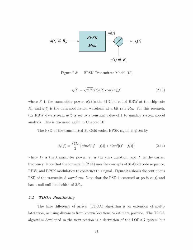
BPSK

Modd(t) @ Rb

c(t) @ Rc

st(t)

m(t)

Figure 2.3: BPSK Transmitter Model [19]

st(t) =√

2Ptc(t)d(t) cos(2πfot) (2.13)

where Pt is the transmitter power, c(t) is the 31-Gold coded RBW at the chip rate

Rc, and d(t) is the data modulation waveform at a bit rate RD. For this research,

the RBW data stream d(t) is set to a constant value of 1 to simplify system model

analysis. This is discussed again in Chapter III.

The PSD of the transmitted 31-Gold coded BPSK signal is given by

St(f) =PtTc

2

{

sinc2[(f + fo)] + sinc2[(f − fo)]}

(2.14)

where Pt is the transmitter power, Tc is the chip duration, and fo is the carrier

frequency. Note that the formula in (2.14) uses the concepts of 31-Gold code sequence,

RBW, and BPSK modulation to construct this signal. Figure 2.4 shows the continuous

PSD of the transmitted waveform. Note that the PSD is centered at positive fo and

has a null-null bandwidth of 2Rc.

2.4 TDOA Positioning

The time difference of arrival (TDOA) algorithm is an extension of multi-

lateration, or using distances from known locations to estimate position. The TDOA

algorithm developed in the next section is a derivation of the LORAN system but

21

Figure 2.4: Transmitted Waveform PSD (Continuous) [19]

differs in that it uses two receivers with one transmitter to estimate the range be-

tween one of the receivers and the transmitter [5]. This range provides a circle in two

dimensions of possible points for the target receiver around the transmitter. There

are two cases of the TDOA concept, TDOA with synchronized receivers and TDOA

with unsynchronized receivers. To better understand the overall picture, this section

concentrates on the less complicated TDOA concept using synchronized receivers.

The two receiver TDOA system requires that the transmitters and one of the

two receivers be static at a known location. The static receiver will be the reference

receiver and it must also have a real-time data link to the second mobile receiver at

the location of interest (target). Given this setup, the time the transmitted signal is

received is recorded at both the mobile and reference receivers. The reference receiver

sends this time of arrival to the target receiver which calculates the time difference

between the signals. This is converted to distance by multiplying by the speed of

light constant. The TDOA measurement is the only measurement needed to estimate

the range between the transmitter and target receiver, as the distance between the

transmitter and reference receiver is known. Since the two receivers are synchronized,

the clock errors will cancel out in the TDOA algorithm.

22

TX

Reference Receiver

Target Receiverttarget

tdifftref TX - Signal Source

- Target Receiver

Propagation Time

- Reference Receiver

Propagation Time

- Time Difference

t

t

t

target

ref

diff

Figure 2.5: Illustration of TDOA Range Estimates [5]

TX 1

TX 2

TX 3

REF

TARGET

REF - Reference ReceiverTARGET - Target ReceiverTX - Signal Sourcedt - Time Difference

dt1

dt2

dt3

Figure 2.6: Illustration of TDOA System with Three SignalSources [5]

23

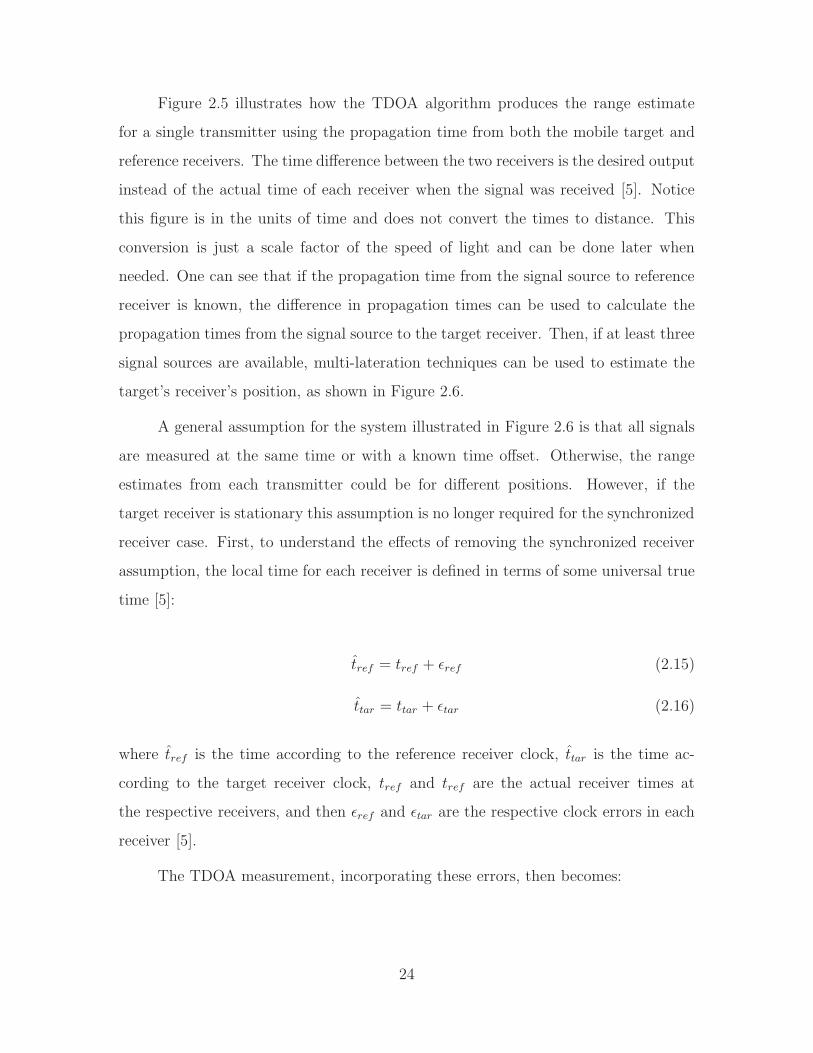
Figure 2.5 illustrates how the TDOA algorithm produces the range estimate

for a single transmitter using the propagation time from both the mobile target and

reference receivers. The time difference between the two receivers is the desired output

instead of the actual time of each receiver when the signal was received [5]. Notice

this figure is in the units of time and does not convert the times to distance. This

conversion is just a scale factor of the speed of light and can be done later when

needed. One can see that if the propagation time from the signal source to reference

receiver is known, the difference in propagation times can be used to calculate the

propagation times from the signal source to the target receiver. Then, if at least three

signal sources are available, multi-lateration techniques can be used to estimate the

target’s receiver’s position, as shown in Figure 2.6.

A general assumption for the system illustrated in Figure 2.6 is that all signals

are measured at the same time or with a known time offset. Otherwise, the range

estimates from each transmitter could be for different positions. However, if the

target receiver is stationary this assumption is no longer required for the synchronized

receiver case. First, to understand the effects of removing the synchronized receiver

assumption, the local time for each receiver is defined in terms of some universal true

time [5]:

t̂ref = tref + ǫref (2.15)

t̂tar = ttar + ǫtar (2.16)

where t̂ref is the time according to the reference receiver clock, t̂tar is the time ac-

cording to the target receiver clock, tref and tref are the actual receiver times at

the respective receivers, and then ǫref and ǫtar are the respective clock errors in each

receiver [5].

The TDOA measurement, incorporating these errors, then becomes:

24

TDOA = t̂tar − t̂ref (2.17)

= (ttar + ǫtar) − (tref + ǫref)

= (ttar − tref) + (ǫtar − ǫref )

=rangeref − rangeref

c+ δt

where t̂tar and t̂ref are the TOAs according to the respective receiver clock, ttar and

tref are the true TOAs, rangetar and rangeref are the actual ranges between the

transmitter and receivers, δt is the difference in clock errors and c is the speed of

light.

Thus, the individual clock errors for each receiver have created an error in the

TDOA measurement. More specifically, the TDOA measurement error is the differ-

ence between the receiver clock errors. If both errors were the same, the measurement

error would be zero. This difference in local clock error is known as the clock bias

and must also be estimated by the TDOA algorithm. The clock bias adds another

unknown causing the required number of range estimates to increase to four for a

three-dimensional position estimate.

Another subtle constraint added by the clock bias is all measurements must be

taken simultaneously. The clock error for each receiver could change over time, and

the TDOA algorithm only estimates a single value for all measurements. Fortunately,

the drift rate statistics of many types of clock are known [5]. If the potential increase

in error caused by this drift over the period in which samples are taken is acceptable,

then the individual measurements can be taken sequentially.

Equation 2.17 defined the TDOA measurement in terms of actual values when

the errors were known. The parameters as known to a physical system can be defined

by rearranging that equation.

25

TDOA =rangetar − rangeref

c+ δt

cTDOA = rangetar − rangeref + cδt

cTDOA + rangeref = rangetar + cδt (2.18)

where cTDOA + rangeref is the “pseudorange-like” measurement, rangetar is the

actual range, and cδt is the clock bias in units of meters.

Note that this is essentially equivalent in form to a GPS pseudorange measure-

ment, which is the combination of true range and clock error [22].

2.5 Summary

This chapter provided the necessary background for the major topics in this

thesis. The basic digital communication concepts needed to construct the 31-Gold

coded BPSK reference signal were presented and discussed. The definition and rel-

evant properties of autocorrelation were also discussed along with the concepts of

TDOA. All the topics discussed in this chapter help with understanding the research

methodology as presented in Chapter III.

26

III. Methodology

This chapter describes the system model and parameters used to evaluate the

correlation characteristics of arbitrary AM and FM radio signals for the purpose

of navigation. Section 3.1 explains the basic model setup and the frontend design of

the receiver model. Section 3.2 discusses the three signal types used in the research

model. Section 3.3 develops two different correlation approaches used for determining

if the signal of interest (SOI) has any correlation characteristics useful for the purpose

of navigation. Section 3.4 clarifies how the term ‘navigation potential of a signal’ is

defined and determined in this research. A summary is given at the end of this

chapter.

3.1 Model Development

Before the Correlation Peak Identifiability (CPI) of a particular SOI can be de-

termined, an accurate model must be developed to analyze and evaluates the acquired

signals. This section discusses the development of the model used for this research.

3.1.1 Basic Model. The basic transmitter and receiver model used in this

research is shown in Figure 3.1. A signal st(t) is transmitted from a known location

through a channel to a target receiver. The transmitted signal st(t) ideally can be

any type of signal. The signal received at the receiver’s antenna sr(t) is the acquired

st(t)

Tx

Transmitter Channel Receiver

AWGN n(t)

Signal Delay

Rx

sr(t)

Figure 3.1: Basic Transmit-Receive Model

27

Correlation

BlockFrontend

Digital

Sampling

Figure 3.2: Major Receiver Components

signal used for potential navigation. A general expression for received signal sr(t) in

terms of transmitted signal st(t) is given by

sr(t) = st(t − Cd) + n(t) (3.1)

where the signal propagation delay Cd and additive-white-gaussian-noise (AWGN)

n(t) factors are included in the received response of (3.1) to make it more realistic.

3.1.2 Receiver Frontend Model. The three major components of the receiver

model are shown in Figure 3.2. The first receiver model component is the frontend.

The purpose to the receiver frontend is to process and convert the high frequency

input signal into a signal that is more suitable for signal processing and analysis. The

receiver frontend model is shown in Figure 3.3. The input signal st(t) is received at

the antenna. The signal is then filtered at a specific radio frequency fRF to extract the

relevant signal energy. The output to HRF is the radio frequency (RF) filtered signal

denoted as sRF . Although a majority of the noise in sRF is filtered out, the signal still

28

exists at the carrier frequency of sr(t). The carrier frequency can be removed using

down conversion. A local oscillator (LO) signal is generated at the carrier frequency

to mix with sRF and down-convert the signal to baseband. The LO signal (sLO) can

be expressed as

sLO = A · cos(2πfct) (3.2)

where A is an arbitrary amplitude, fc is the carrier frequency and t is the time.

Mixing sRF and sLO produces the In-phase (I) signal response xI(t) given by.

xI(t) = sRF · A cos(2πfct) (3.3)

By phase shifting sLO by 90 degrees, the Quadrature-phase (Q) signal response

xQ(t) is generated. Accounting for these changes in Equation 3.2 and Equation 3.3

yields the following:

sLO = A · sin(2πfct) (3.4)

xQ(t) = sRF · A sin(2πfct) (3.5)

Once the In-phase and Quadrature (I&Q) mixed signals are produced, the

signals are filtered through a baseband (BB) filter (HBB) to complete the down-

conversion process. At this point, the received RF signal exists at a baseband fre-

quency. The output signals from the HBB filters are the I&Q experimental data. The

I&Q experimental data is denoted as zI(t) and zQ(t), respectively. This receiver fron-

tend process filters, mixes and filters the input signal down to the baseband frequency

where it is digitally sampled. The frontend process is called ‘conditioning the received

signal’. Note that the digital sampling process is the second of three major receiver

model components shown in Figure 3.2.

29

HRF

sr(t)

HBB

HBB

LO90°

WBB

@ fBB

WRF

@ fRF

sRF

WBB

@ fBB

sLO

zI(t)

zQ(t)

xI(t)

xQ(t)

I&Q

Experimental

Data

Figure 3.3: Receiver Frontend Model

The filters in this model were designed based on the specifications of each SOI.

One type of filter was used in this research, the finite impulse response (FIR) 2nd-

Order Butterworth filter. This selection was made based on ease of implementation in

simulation. There are other advanced filters which exist that have better character-

istics such as sharper transitions between passband and stopband, more attenuation

and less ripple in the stopband, and less phase delay [5]. However, using such an

advanced filter was not necessary for the scope of this research. High fidelity filter

characteristics, such as the precise bandstopping capability at the edges of the pulses,

were not critical to evaluating overall system performance. The filters were designed

to induce general effects of bandlimiting the signal while capturing a majority of the

signal energy within the filter bandwidth. Problems that usually arise from using

FIR filters such as Gibbs phenomenon or ringing at discontinuities did not have an

extreme affect on the process [5]. If the research required, the phenomenon can be

reduced by windowing, but it can never be completely eliminated in FIR filters. There

are other filters that avoid this phenomenon, such as infinite impulse response (IIR)

filters, but with the tradeoff of increased signal processing [15].

30

3.2 Signal Types

There are three different signal types used in this research. The three SOIs

considered include a 31-Gold coded random binary waveform (RBW), the AM radio

waveform and the FM radio waveform. The structure and details for each of the

waveforms are given in the following subsections.

3.2.1 31-Gold Coded Random Binary Waveform. The first step in determin-

ing the accuracy and functionality of a designed system model is to test the process

with a known input and analyze the results of the output. The known input for this

research is a 31-Gold Coded RBW. The statistics for the spreading waveform C(t)

used to construct the RBW are given in Table 3.1. Note that one second of the

spreading waveform contains one symbol, there are 31 chips/symbol, with 50 sam-

ples/chip, and thus a total of 1550 data samples/symbol. The number of symbols in

the waveform used for this simulation was set at 3 symbols. This number is somewhat

arbitrary and was set based on simulation capability.

The equation for a 31-Gold coded RBW is shown in Equation 3.6 [8] which not

only contains the spreading code but also the information data stream d(t) and the

noise

sRBW = C(t)d(t) cos(2πfct) + n(t) (3.6)

where C(t) is the spreading waveform, d(t) is the information data stream, fc is the

carrier frequency, t is the time, and n(t) is the AWGN.

The 31-Gold coded RBW is the initial signal used to test the integrity of the

system model. For analysis purposes, the information data d(t) was set equal to a

constant value of 1. This simplification reduces Equation 3.6 to

sRBW = C(t) cos(2πfct) + n(t) (3.7)

31

Table 3.1: Statistics of 31-Gold Spreading CodeStatistics Value

Number of Chips per Symbol 31Symbol Duration 1.0 secChip Duration 0.0323 secs

Samples per Chip 50Carrier Frequency fc 155 Hz

Time between Samples △t 6.4516e-4 secsSample Frequency fs 1550 Hz

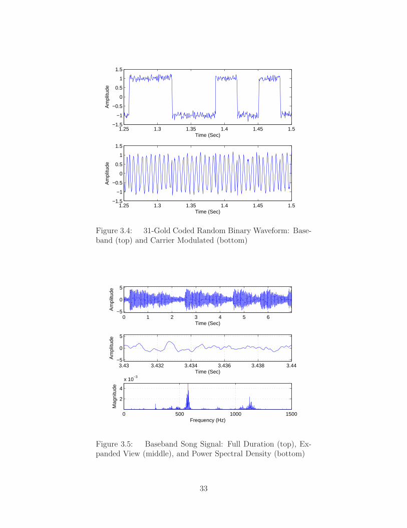
A segment of the signals are shown in Figure 3.4. The top plot shows the C(t)-

plus-noise signal and the bottom plot shows the carrier modulated C(t)-plus-noise

signal. Note the corresponding sign changes between the RBW and the final received

signal. This carrier modulated RBW is used as the initial verification signal because

the structure of the waveform and its correlation characteristics are known, i.e., the

received signal is a periodic waveform with a known spreading code modulated onto it.

The known properties and structures of this input signal allows the user to predict the

model results. If the actual results are consistent with the expected results, then the

user can are confident that the system model is performing as designed (verification).

3.2.2 AM and FM Radio Waveforms. The AM and FM radio signals used

in this research were created by taking real baseband data (voice and song) and then

modulating the data onto a carrier using software to simulate the real-world radio

signals. The baseband data was stored in a *.wav data format. The normalized

baseband song and voice signals are shown in Figure 3.5 and Figure 3.6, respectively.

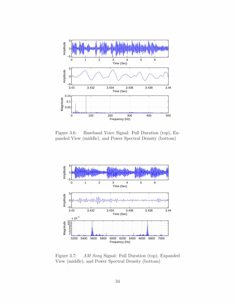
In these figures, the top plot is the full time duration of the signals, the middle plot is

a zoomed-in version and the bottom plot is the power spectral density (PSD). Using

MatlabR©, the data for both the voice and song baseband signals were amplitude and

frequency modulated as described in the following subsections.

32

1.25 1.3 1.35 1.4 1.45 1.5−1.5

−1

−0.5

0

0.5

1

1.5

Time (Sec)

Am

plitu

de

1.25 1.3 1.35 1.4 1.45 1.5−1.5

−1

−0.5

0

0.5

1

1.5

Time (Sec)

Am

plitu

de

Figure 3.4: 31-Gold Coded Random Binary Waveform: Base-band (top) and Carrier Modulated (bottom)

0 1 2 3 4 5 6−5

0

5

Time (Sec)

Am

plitu

de

3.43 3.432 3.434 3.436 3.438 3.44−5

0

5

Time (Sec)

Am

plitu

de

0 500 1000 1500

2

4

x 10−3

Frequency (Hz)

Mag

nitu

de

Figure 3.5: Baseband Song Signal: Full Duration (top), Ex-panded View (middle), and Power Spectral Density (bottom)

33

0 1 2 3 4 5 6−5

0

5

Time (Sec)A

mpl

itude

3.43 3.432 3.434 3.436 3.438 3.44−5

0

5

Time (Sec)

Am

plitu

de

0 100 200 300 400 500

0.05

0.1

0.15

Frequency (Hz)

Mag

nitu

de

Figure 3.6: Baseband Voice Signal: Full Duration (top), Ex-panded View (middle), and Power Spectral Density (bottom)

0 1 2 3 4 5 6−5

0

5

Time (Sec)

Am

plitu

de

3.43 3.432 3.434 3.436 3.438 3.44−5

0

5

Time (Sec)

Am

plitu

de

5200 5400 5600 5800 6000 6200 6400 6600 6800 7000

2468

1012

x 10−4

Frequency (Hz)

Mag

nitu

de

Figure 3.7: AM Song Signal: Full Duration (top), ExpandedView (middle), and Power Spectral Density (bottom)

34

0 1 2 3 4 5 6−5

0

5

Time (Sec)

Am

plitu

de

3.43 3.432 3.434 3.436 3.438 3.44−5

0

5

Time (Sec)

Am

plitu

de

5200 5400 5600 5800 6000 6200 6400 6600 6800 7000

123

x 10−3

Frequency (Hz)

Mag

nitu

de

Figure 3.8: AM Voice Signal: Full Duration (top), ExpandedView (middle), and Power Spectral Density (bottom)

3.2.2.1 AM Radio Waveform. Amplitude modulation (AM) is the

technique of varying the amplitude, or strength, of a radio signal in accordance to the

voice or music being transmitted [11]. The interest in using the AM radio signal as

a SOI is based on the fact that AM radio technology is available world-wide and the

coverage of AM frequencies is broader than FM radio.

AM radio signals are electromagnetic waves with frequencies between 535 kHz

and 1605 kHz [12]. However the obtained baseband data was sampled at a frequency

of 24576 Hz. And the carrier frequency must be at most half the sampling frequency.

So for testing and simulation purposes, the normalized baseband data was modulated

at fourth of the sampling frequency, 6144 Hz.

Figure 3.7 and Figure 3.8 are the AM normalized baseband song and voice

data, respectively. The top plot shows the entire AM song signal while the middle

plot shows the zoomed-in version. The bottom plot shows the PSD.

35

3.43 3.432 3.434 3.436 3.438 3.44−1

−0.5

0

0.5

1

Time (Sec)

Am

plitu

de

0 2000 4000 6000 8000 10000 12000

2

4

6

x 10−5

Frequency (Hz)

Mag

nitu

de

Figure 3.9: FM Song Signal: Full Duration (top), ExpandedView (middle), and Power Spectral Density (bottom)

3.2.2.2 FM Radio Waveform. Frequency modulation (FM) is the

technique of varying the frequency of a radio signal in accordance to the voice or

music being transmitted [11]. The interest in using the FM radio signal as a SOI is

based on the fact that the overall trend of FM radio signals are better quality than

AM radio signals. FM radio signals have less susceptible to static which hopefully

corresponds with higher potential for navigation.

FM radio signals are electromagnetic waves with frequencies between 88 MHz

and 108 MHz [12]. However the obtained baseband data was sampled at a frequency

of 24576 Hz. And the carrier frequency must be at most half the sampling frequency.

So for testing and simulation purposes, the normalized baseband data was modulated

at fourth of the sampling frequency, 6144 Hz.

Figure 3.9 and Figure 3.10 are the FM normalized baseband song and voice

data, respectively. The top plot shows the entire AM song signal while the middle

plot shows the zoomed-in version. The bottom plot shows the PSD.

36

3.43 3.432 3.434 3.436 3.438 3.44−1

−0.5

0

0.5

1

Time (Sec)

Am

plitu

de

0 2000 4000 6000 8000 10000 12000

2

4

6

8x 10

−5

Frequency (Hz)

Mag

nitu

de

Figure 3.10: FM Voice Signal: Full Duration (top), ExpandedView (middle), and Power Spectral Density (bottom)

3.3 Correlator Development

The third and final major component of the receiver shown in Figure 3.2 is the

correlation block. Once the receiver has conditioned the received signal by filtering the

noise and removing the carrier, the data can be stored and correlated with data from

another receiver. Navigation is done by determining the TDOA between two receivers’

data as discussed in Section 2.4. The two different correlation approaches shown in

this section are designed to account for multiple delay values which correspondingly

simulate multiple receivers at different locations.

3.3.1 Correlation A: “Varying” Reference Correlation. The first correlation

approach is referred to as the “varying-reference” method. The varying reference

corresponds to changing correlation window when each correlation iteration is being

done. This correlation method is depicted in the diagram shown in Figure 3.11 where

Nw is the width of the correlation window and ∆w is the number of samples shifted

between correlation calculations. In this case, the input signal z(t) is multiplied by

37

z (t)

Nd

CorrelationA

Window Width: Nw

Shift Value: w

(REFERENCE Rx)

(TARGET Rx)

Figure 3.11: Correlation A - “Varying” Reference Correlation

the delayed version of itself z(t − TD). The undelayed and delayed signals represent

the received signals from the reference and target receivers, respectively. Once the two

signals are multiplied, correlation between the delayed and undelayed signal can be

determined. This method of correlation is intended to represent a real-time (analog)

correlation process.

The best way to explain how the Correlation A process was designed is operate is

via example as shown in Figure 3.12. The undelayed signal is shown by sample indexes.

The delayed signal is delayed by 3 samples (Nd) and shown below the undelayed signal.

The two signals are then multiplied sample-by-sample. After multiplication, the first

correlation value at iteration i = 1 is calculated by summing up the samples within a

correlation window. The correlation window size (Nw) is indicated by the shaded area

which is Nw = 5 samples for this example. The next correlation value for iteration

i = 2 is calculated after shifting the correlation window by ∆w samples. The process

of shifting the correlation window between iterations is why the terminology “varying”

reference is applied to this correlation method. The shift value of the window (∆w) is

set to 1 for this example. So for a total signal length of (Ni), the correlation window

is shifted or “varied” by ∆w between each correlation iteration until all Ni values

have been correlated across. This model is designed to account for multiple delays

(variable ‘Nd’ in Figure 3.11) which simulate multiple locations of the target receivers.

38

1 2 3 4 5 6 7 8 9 10 11 12 …x_undelay

x_delay

Example: Nd = 3, Nw = 5 and w = 1

i = 1

varying reference Nw = 5

t1 t2 t3 t4 t5 t6 t7 t8 t9 … tNi

1 2 3 4 5 6 7 8 9 …

.

.

.

.

.

.

time index

1 2 3 4 5 6 7 8 9 10 11 12 …

i = 2

shift w = 1

1 2 3 4 5 6 7 8 9 …

1 2 3 4 5 6 7 8 9 10 11 12 …

i = 3

shift w = 1

1 2 3 4 5 6 7 8 9 …

Figure 3.12: Example Illustrating Three Iterations of “Vary-ing” Reference Correlation

CorrelationB

Window Width: NW

Shift Value: w

Store

Nw

z (t) Nd(TARGET Rx)

(REFERENCE Rx)

Figure 3.13: Correlation B - “Fixed” Reference Correlation

39

1 2 3 4 5 6 7 8 9 10 11 … Ni

1 2 3 4 5 6 7 8 … Ni

x_undelay

x_delay

Example: Nd = 3, Nw = 5 and w = 1

i = 1

i = 2

i = 3

reference Nw = 5

t1 t2 t3 t4 t5 t6 t7 t8 t9 … tNi

1 2 3 4 5 6 7 8 … Ni

1 2 3 4 5 6 7 8 … Ni

.

.

.

.

.

.

time index

delay Nd =3

shift w = 1

Figure 3.14: Example Illustrating Three Iterations of “Fixed”Reference Correlation

3.3.2 Correlation B: “Fixed” Reference Correlation. The second correlation

approach is referred to as the “fixed-reference” method. The fixed reference corre-

sponds to the fixed correlation reference window when each correlation iteration is

being done. This correlation method is depicted in the diagram shown in Figure 3.13.

In this case, an Nw segment of the undelayed signal is stored (fixed-reference win-

dow) and used as a reference correlation signal across the entire delayed signal. The

undelayed signal represents the signal from the reference receiver. The delayed signal

represents the signal from the target receivers. Once the fixed-reference window is

stored, correlation between the fixed-reference and the delayed signal can be deter-

mined.

The best way to explain how the Correlation B process was designed to operate

is via example. Three iterations of the fixed-reference correlation method is shown in

Figure 3.14. The example shows the fixed-reference being set to the first 5 samples of

the undelayed signal. For the first i = 1 iteration the correlation value is calculated

by multiplying and summing up the samples within a correlation window. The corre-

lation window size (Nw) is indicated by the shaded area which is Nw = 5 samples for

this example. The next correlation value for the i = 2 iteration is calculated by taking

the same fixed-reference window and shifting it to the right along the delayed signal

40

by ∆w. The notion of keeping the same reference window and shifting along the de-

layed signal between iterations is why the “fixed” reference terminology is applied to

this correlation method. The window shift value (∆w) is set to 1 for this example. So

for a total length data signal of Ni samples, the fixed-correlation window is shifted by

∆w between each correlation iteration until all Ni values have been correlated across.

This model is designed to account for multiple delays (variable ‘Nd’ in Figure 3.13)

which simulate multiple target receiver locations.

3.4 Definition of Navigation Potential

The main concept for this research is derived from the concepts developed in [5,7]

however the methodology and results between this thesis and the work done in [5, 7]

are quite different. The main difference between this research and [5,7] is the definition

of ‘navigation potential’. The research in [5,7] already assumes the user knows which

correlation peak is being tracked so that ‘navigation potential’ could be defined as the

accuracy with which the user could estimate the time difference between a reference

and target receiver. Navigation potential in this research is determined by how well the

user will be able to distinguish and locate the correct correlation peak, or Correlation

Peak Identifiability (CPI). In the real world, both the ability to locate the correct

correlation peak and the ability to get accurate estimates of the time delay between

the reference and target receivers are needed for navigation.

The navigation potential of the signals presented in Chapter IV will be based on

one determining factor. The signal will be categorized as ‘promising potential’ if any

arbitrary segment of the signal can be used to produce a distinguishable autocorrela-

tion peak. Otherwise the signal will be categorized as ‘limited potential’. Navigation

potential in this research will interpreted as the ability to distinguishably locate the

correct autocorrelation peak, CPI, regardless of the signal segment selected. Again,

note this is not the same definition used in [5, 7].

41

3.5 Summary

This chapter describes the overall transmit-receiver system model and param-

eters used to evaluate the CPI of the AM and FM radio signals for the purpose of

navigation. The basic model setup and the receiver frontend design were discussed

as well as the three signal types used in the research. Two different correlation ap-

proaches were introduced for determining if the signals of interest have any navigation

potential. The term ‘navigation potential’ and CPI are also defined to help clarify

the conclusions drawn from the Chapter IV.

42

IV. Simulation Results and Analysis

This chapter presents simulated results and analysis conducted with the receiver

model and two correlation methods described in Section 3.1 and Section 3.3,

respectively. Section 4.1 provides model verification by presenting and analyzing

simulation results for the 31-Gold Coded RBW signal. Section 4.2 shows and discusses

the results of the model when AM radio signals are used as the input waveform.

Section 4.3 repeats the analysis but for FM radio signals as the input waveform. Each

radio signal section conducts an analysis with both song and voice type waveforms and

both correlation methods. The correlation results will help determine if navigation is

possible for each case.

4.1 Model Verification

Before the CPI of a particular SOI can be determined for the purpose of nav-

igation, an accurate model must be developed to analyze and evaluate the acquired

signals. This section shows the model results when using the periodic 31-Gold coded

RBW as the input signal. Due to the known characteristics of the signal, the actual

results can be compared to the theoretical results to verify the model’s process. The

validation results are shown in this section and organized into three parts. The parts

are represented as frontend results, correlation method results when varying delay

and correlation method results when varying correlation window size. Correlation

method results are shown in raw and normalized-dB scale forms.

4.1.1 Frontend Model Results and Analysis. The following results are pre-

sented to verify the frontend process. As designed, the frontend model performs well

in conditioning the received signal into a noise-reduced baseband signal. The process

is similar for all of the correlation-waveform type cases so only one set of step-by-

step results and analysis are discussed. For the remainder of the frontend process

results, only the signals before and after the conditioning process will be shown. The

filter bandwidths used in the simulation for each signal are summarized in Table 4.1.

43

Figure 4.1: Frontend Process - RF Filter Results

Figure 4.2: Frontend Process - Downconversion and BB FilterResults

44

Table 4.1: Bandwidth for Frontend Process FiltersSignal Type HRF HBB

31-Gold coded RBW 101 Hz 99 HzAM Song 1057 Hz 1044 HzAM Voice 161 Hz 162 HzFM Song 2114 Hz 2088 HzFM Voice 322 Hz 324 Hz

Note that the center frequency used for the passband HRF filters was 155 Hz for the

31-Gold coded RBW signal and 6144 Hz for the AM and FM radio signals.

The frontend process is validated by using the 31-Gold coded signal as the

input waveform. Figure 4.1 shows the results for the RF filter portion of the frontend

process. The top row of figures are the received signal and PSD of the received signal.

The received signal appears noise-like but the PSD shows a majority of signal energy

centered approximately around 155 Hz. This result makes sense since the carrier wave

frequency was set to 155 Hz in the simulation. The bottom row of figures show the

RF filter response and the PSD of the received signal after the RF filter. The RF

filter used, as mentioned in Section 3.1, is a 2nd-order Butterworth filter. Note the

PSD of the received signal before and after RF filtering. The after-picture reveals

the before-PSD with a majority of the original energy but without some of the noise

spikes. This result indicates that the filter performs as designs and removes unwanted

noise.

Figure 4.2 shows results for the down-conversion and BB filtering portion of

the frontend process. The top row of figures are the received signal PSD after down-

conversion process and the BB filter response. Note that the top-left figure shows that

down conversion is operating correctly in the simulation. The figure correctly shows

that the signal PSD after the RF filter is now centered at baseband with spectral

replicas appearing at ±2 × fc and having one-half the PSD magnitude. The BB

filter, as mentioned in Section 3.1, is a 2nd-order Butterworth filter. The bottom

plots in Figure 4.2 are the received signal PSD after BB filtering and the received

signal after the frontend process. Note the before and after BB filtered PSD of the

45

down-converted signal. The after-picture reveals the filtered down converted signal

without the higher frequency components. The PSD after BB filtering shows only the

PSD centered around 0 Hz. This result indicates that the filter performed as designed

by removing the unwanted components. The lower right-hand plot in Figure 4.2

shows approximately the same 31-Gold coded RBW as constructed (Figure 3.4) before

carrier modulation. This final figure demonstrates that the conditioning process does

perform successfully in removing channel noise and removing the carrier frequency.

4.1.2 Correlation Methods - Varying Sample Delay Nd. The correlation

methods discussed in Section 3.3 have three variables that are under the user’s control

for each signal type. The three variables are the correlation window width Nw, the

signal delay Nd, and the step size between correlation iterations ∆w. For ease of data

presentation and comprehension, two of the three variables are held fixed. So for this

research, Nd is varied while Nw and ∆w are held constant. Note ∆w controls the

resolution of the output data. For best resolution, ∆w is set to the smallest value of

∆w = 1 for this work. For verification with the RBW signal, Nw is set equal to one

full period of the RBW, or 1550 samples. The results for correlation methods A and

B when varying Nd are provided in the following subsections.

4.1.2.1 Correlation-A with 31-Gold Code RBW Signal. Results for

the Correlation-A method using the 31-Gold coded RBW signal when varying Nd

are shown in Figure 4.3. This figure represents the ‘varying’ reference correlation

approach where Nw = 1550 samples and ∆w = 1. By varying Nd (y-axis), correlation

is done as describe in Section 3.3. The correlation window of 1550 samples is shifted

by 1 between iterations and repeated for all the delay values. The correlation output

for various delays values constructs the data matrix shown in Figure 4.3. Recall from

Section 3.2 that the input RBW signal is periodic every 1550 samples. This explains

the characteristic correlation peaks appearing in Figure 4.3 at shift values equaling

integer multiples of 1550 samples (Delay = 0 and Delay = 1550). The max peaks

represent the autocorrelation value. These results are consistent with the model and

46

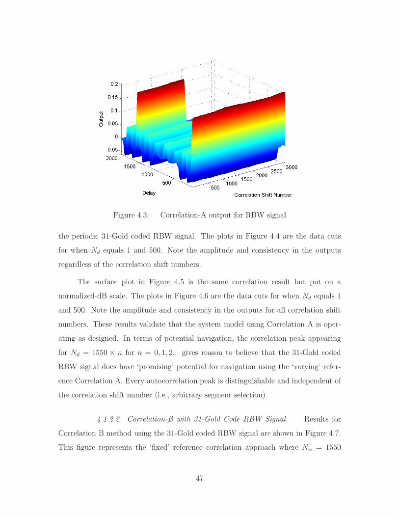
Figure 4.3: Correlation-A output for RBW signal

the periodic 31-Gold coded RBW signal. The plots in Figure 4.4 are the data cuts

for when Nd equals 1 and 500. Note the amplitude and consistency in the outputs

regardless of the correlation shift numbers.

The surface plot in Figure 4.5 is the same correlation result but put on a

normalized-dB scale. The plots in Figure 4.6 are the data cuts for when Nd equals 1

and 500. Note the amplitude and consistency in the outputs for all correlation shift

numbers. These results validate that the system model using Correlation A is oper-

ating as designed. In terms of potential navigation, the correlation peak appearing

for Nd = 1550 × n for n = 0, 1, 2... gives reason to believe that the 31-Gold coded

RBW signal does have ‘promising’ potential for navigation using the ‘varying’ refer-

ence Correlation A. Every autocorrelation peak is distinguishable and independent of

the correlation shift number (i.e., arbitrary segment selection).

4.1.2.2 Correlation-B with 31-Gold Code RBW Signal. Results for

Correlation B method using the 31-Gold coded RBW signal are shown in Figure 4.7.

This figure represents the ‘fixed’ reference correlation approach where Nw = 1550

47

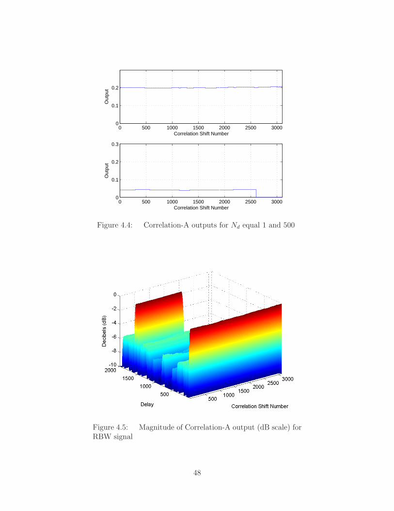
0 500 1000 1500 2000 2500 30000

0.1

0.2

Correlation Shift Number

Out

put

0 500 1000 1500 2000 2500 30000

0.1

0.2

0.3


Out

put

Figure 4.4: Correlation-A outputs for Nd equal 1 and 500

Figure 4.5: Magnitude of Correlation-A output (dB scale) forRBW signal

48

0 500 1000 1500 2000 2500 3000−10

−8

−6

−4

−2

0

2


Dec

ibel

s (d

B)

0 500 1000 1500 2000 2500 3000−10

−8

−6

−4

−2

0

2


Dec

ibel

s (d

B)

Figure 4.6: Magnitude of Correlation-A outputs (dB scale)for Nd equal 1 and 500

Figure 4.7: Correlation-B output for RBW signal

49

0 500 1000 1500 2000 2500 3000−0.1

0

0.1

0.2

0.3


Out

put

0 500 1000 1500 2000 2500 3000−0.1

0

0.1

0.2

0.3


Out

put

Figure 4.8: Correlation-B outputs for 100th and 749th refer-ence window

Figure 4.9: Magnitude of Correlation-B output (dB scale) forRBW signal

50

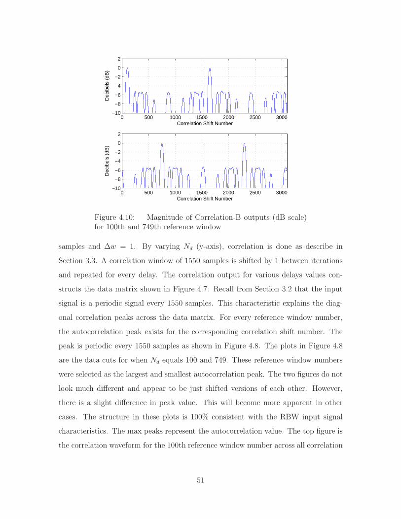
0 500 1000 1500 2000 2500 3000−10

−8

−6

−4

−2

0

2


Dec

ibel

s (d

B)

0 500 1000 1500 2000 2500 3000−10

−8

−6

−4

−2

0

2


Dec

ibel

s (d

B)

Figure 4.10: Magnitude of Correlation-B outputs (dB scale)for 100th and 749th reference window

samples and ∆w = 1. By varying Nd (y-axis), correlation is done as describe in

Section 3.3. A correlation window of 1550 samples is shifted by 1 between iterations

and repeated for every delay. The correlation output for various delays values con-

structs the data matrix shown in Figure 4.7. Recall from Section 3.2 that the input

signal is a periodic signal every 1550 samples. This characteristic explains the diag-

onal correlation peaks across the data matrix. For every reference window number,

the autocorrelation peak exists for the corresponding correlation shift number. The

peak is periodic every 1550 samples as shown in Figure 4.8. The plots in Figure 4.8

are the data cuts for when Nd equals 100 and 749. These reference window numbers

were selected as the largest and smallest autocorrelation peak. The two figures do not

look much different and appear to be just shifted versions of each other. However,

there is a slight difference in peak value. This will become more apparent in other

cases. The structure in these plots is 100% consistent with the RBW input signal

characteristics. The max peaks represent the autocorrelation value. The top figure is

the correlation waveform for the 100th reference window number across all correlation

51

shift iterations. Note the peaks occurring every 1550 samples starting from the 100th

correlation shift number. The bottom figure is the same correlation but using the

749th reference window. Note the peaks occurring every 1550 samples starting from

the 749th correlation shift number. It is also important to note that the non-peak

responses are effectively three-valued, which is consistent with the three-valued cross-

correlation characteristics inherent in RBWs. These results are consistent with the

model and the periodic 31-Gold coded RBW signal.


normalized-dB scale. The plots in Figure 4.10 are the data cuts for when Nd equals

100 and 749. Note the amplitude and consistency in the outputs for all correlation

shift numbers. These results validate that the system model using Correlation B is

operating as designed. In terms of potential navigation, the correlation peak appears

for all values Nd for some correlation shift number, regardless of which reference win-

dow used. The property suggests that the 31-Gold coded RBW signal has ‘promising’

potential for navigation using the ‘fixed’ reference Correlation B. Every autocorrela-

tion peak is distinguishable and independent of the reference correlation number (i.e.,

arbitrary segment selection).

4.1.3 Correlation Methods - Varying Correlation Window Size Nw. For

ease of data presentation and comprehension, two of three controllable variables in

the correlation methods are held fixed. As mentioned before, the value for Nd is

varied while Nw and ∆w are held constant for this research. Note ∆w controls the

resolution of the output data and for best resolution, ∆w is set to the smallest value

which is 1. The Nw is set to one full period which is 1550 samples however for non-

periodic signals, an optimum window size needs to be determined. So the following

results tested what would happen if Nw were varied instead of Nd. The results for

correlation methods A and B when varying Nw are shown below. Notice that only

results for the 31-Gold coded RBW signal when varying correlation window size are

shown. The simulations for all the other signals were performed with a majority of

52

Figure 4.11: Correlation-A output for RBW signal when vary-ing Nw

the results showing the same overall trend. After this section, the remainder of the

research and results presented herein only deal with the correlation methods having

varying delay and not window sizes. For this research, the correlation window sizes

were selected to be large enough to give meaningful results.

4.1.3.1 Correlation-A with 31-Gold Code RBW Signal. Results for

Correlation A using the 31-Gold coded RBW signal when varying Nw is shown in

Figure 4.11. This figure represents the ‘varying’ reference correlation approach where

Nd = 10 samples and ∆w = 1. By varying Nw (y-axis), correlation is done as describe

in Section 3.3. The correlation window size is varied and is shifted by 1 sample

between iterations and repeated for all the correlation window sizes. The correlation

output for various window sizes constructs the data matrix shown in Figure 4.11.

The variable Nd was set to 10 samples because this case showed the overall trend the

best. Figure 4.11 shows that for correlation method A, larger windows correspond to

larger correlation amplitudes. So the selection of Nw = 1550 was a workable value and

provided adequate results. Remember from Section 2.2 that, in general, the larger

53

Table 4.2: Nw and ∆w Values of Correlation-ASignal Type Nw ∆w

31-Gold coded RBW 1550 1AM Song 1000 1000AM Voice 1000 1000FM Song 1000 1000FM Voice 1000 1000

Figure 4.12: Correlation-B output for RBW signal when vary-ing Nw

the correlation window, a better correlation value will be given. This characteristic

explains the increasing correlation output peak value as the correlation window size

increases. There is a direct connection between the size of the correlation window and

the amplitude of the autocorrelation peak. So as long as the results were meaningful,

the user may use any correlation window size. The values for Nw and ∆w used for

correlation method A are summarized in Table 4.2.

4.1.3.2 Correlation-B with 31-Gold Code RBW Signal. The result for

the Correlation-B method using the 31-Gold coded RBW signal when varying Nw is

shown in Figure 4.12. This figure represents the ‘fixed’ reference correlation approach

54

Table 4.3: Nw and ∆w Values of Correlation-BSignal Type Nw ∆w

31-Gold coded RBW 1550 1AM Song 1000 1AM Voice 1000 1FM Song 1000 1FM Voice 1000 1

where Nd = 10 samples and ∆w = 1. By varying Nw (y-axis), correlation is done as

describe in Section 3.3. The correlation window size is varied and is shifted by 1 sample

between iterations and repeated for all the correlation window sizes. The correlation

output for various window sizes constructs the data matrix shown in Figure 4.12.

The variable Nd was set to 10 samples because this case showed the overall trend the

best. Figure 4.12 shows that for correlation method B, larger windows correspond

with larger correlation amplitude. So the selection of Nw = 1550 was a workable

value. This characteristic explains the increasing correlation output peak value as the

correlation window size increase. There is a direct connection between the size of the

correlation window and the amplitude of the autocorrelation peak. So as long as the

results were meaningful, the user may use any correlation window size. The values

for Nw and ∆w used for correlation method B are summarized in Table 4.3.

4.2 AM Radio Signal

The results shown in this section are for the AM radio signal. The results are

organized by frontend results, Correlation-A results with song and voice signals, and

Correlation-B results with song and voice signals. The frontend results are shown to

verify that the signal out of the BB filter is the desired signal. The correlation results

are shown by varying the signal delay. The results for the correlation process are

organized into three plots. The first plot is the raw correlation data. The second plot

is the normalized-dB scaled correlation data. And the last plot takes the cuts from

the largest and smallest autocorrelation peak of the normalized-dB scaled data. The

results are repeated for each correlation method and each signal data type.

55

0 1 2 3 4 5 6 7−5

0

5

Time (Sec)

Am

plitu

de

0 1 2 3 4 5 6 7−5

0

5

Time (Sec)

Am

plitu

de

Figure 4.13: Conditioned AM song signal - Received (top)and Down-Converted (bottom) signal

4.2.1 AM Song Signal Results and Analysis. There are two types of data

signals used in this research. The two data types are song and voice. The following

results deal with the AM song signal as the input to the system model.

4.2.1.1 Frontend Process Results for AM Song Results. Figure 4.13

verifies that the frontend process is operating correctly. The top plot in Figure 4.13

is the received AM song signal where the bottom plot is the down-converted output

signal from the frontend process. The before and after plots shows what the received

signal looks like without the channel noise and the carrier frequency. The conditioned

signal is the signal used for correlation.

4.2.1.2 Correlation-A with AM Song Signal. The result for the Correlation-

A method using the AM song signal when varying Nd is shown in Figure 4.14. This

figure represents the ‘varying’ reference correlation approach where Nw = 1000 sam-

ples and ∆w = 1000. The ∆w is set to 1000 samples to simulate a real-time process.

By varying Nd (y-axis), correlation is done as describe in Section 3.3. The correlation

56

Figure 4.14: Correlation-A output for AM song signal

Figure 4.15: Magnitude of Correlation-A output (dB scale)for AM song signal

57

0 20 40 60 80 100 120 140 160−10

−8

−6

−4

−2

0

2


Dec

ibel

s (d

B)

0 20 40 60 80 100 120 140 160−10

−8

−6

−4

−2

0

2


Dec

ibel

s (d

B)

Figure 4.16: Magnitude of Correlation-A outputs (dB scale)for 1st and 500th reference window

window of 1000 samples is shifted by 1000 between iterations and repeated for all

the delay values. The correlation output for various delays values constructs the data

matrix shown in Figure 4.14. The max peaks are suppose to represent the autocor-

relation value. This plot does have distinguished max peaks. The max peaks occur

when Nd = 0 which makes sense since this is the definition of autocorrelation.


normalized-dB scale. Putting the data on a dB-scale provides another comparison by

looking at relative power. The plots in Figure 4.16 are the data cuts for when Nd

equals 1 and 500. Note the varying amplitudes within each plot and the difference in

amplitude between the plots. The correlation peak only appears sporadically when

Nd = 0. And when Nd = 0, the magnitude of the autocorrelation peak varies and is

now dependent on the correlation shift number. This inconsistent trend gives reason

to believe that the AM song signal only has ‘limited’ potential for navigation using

the ‘varying’ correlation method A. A distinguishable autocorrelation peak does not

occur for every arbitrary segment selection.

58

Figure 4.17: Correlation-B output for AM song signal

Figure 4.18: Magnitude of Correlation-B output (dB scale)for AM song signal

59

0 500 1000 1500 2000

−4

−2

0

2


Dec

ibel

s (d

B)

0 500 1000 1500 2000

−4

−2

0

2


Dec

ibel

s (d

B)


4.2.1.3 Correlation-B with AM Song Signal. The result for the Correlation-

B method using the AM song signal is shown in Figure 4.17. This figure represents

the ‘fixed’ reference correlation approach where Nw = 1000 samples and ∆w = 1.

By varying Nd (y-axis), correlation is done as describe in Section 3.3. A correlation

window of 1000 samples is shifted by 1 between iterations and repeated for every ref-

erence window number. The correlation output for various delay values constructs the

data matrix shown in Figure 4.17. For every reference window, the autocorrelation

peak exists for the corresponding correlation shift number. The autocorrelation peak

is expected to be seen on the diagonal of the data matrix. However there are other

peaks not on the diagonal that are relatively close in amplitude.




equals 9 and 1635. These reference window numbers were selected as the largest and

smallest autocorrelation peak. Note the varying amplitudes within each plot and the

60

0 1 2 3 4 5 6 7−5

0

5

Time (Sec)

Am

plitu

de

0 1 2 3 4 5 6

−0.5

0

0.5

Time (Sec)

Am

plitu

de

Figure 4.20: Conditioned AM voice signal - Received (top)and Down-Converted (bottom) signal

difference in amplitude between the plots. In terms of potential navigation, the actual

autocorrelation peak is difficult to identify because there are too many peaks within

2dB of each other. This undistinguishable result gives reason to believe that the AM

song signal only has ‘limited’ potential for navigation using the ‘fixed’ correlation

method B. An autocorrelation peak does occur for every arbitrary segment selection

but it is not definitely distinguishable.

4.2.2 AM Voice Signal Results and Analysis. There are two types of data


results deal with the AM voice signal as the input to the system model.

4.2.2.1 Frontend Process Results for AM Voice Results. Figure 4.20


is the received AM voice signal where the bottom plot is the down-converted output


61

Figure 4.21: Correlation-A output for AM voice signal



4.2.2.2 Correlation-A with AM Voice Signal. The result for the

Correlation-A method using the AM voice signal when varying Nd is shown in Fig-

ure 4.21. This figure represents the ‘varying’ reference correlation approach where

Nw = 1000 samples and ∆w = 1000. The ∆w is set to 1000 samples to simulate

a real-time process. By varying Nd (y-axis), correlation is done as describe in Sec-

tion 3.3. The correlation window of 1000 samples is shifted by 1000 between iterations

and repeated for all the delay values. The correlation output for various delays values

constructs the data matrix shown in Figure 4.21. The max peaks are suppose to

represent the autocorrelation value. This plot does have distinguished max peaks.

The max peaks occur when Nd = 0 which makes sense since this is the definition of

autocorrelation.


normalized-dB scale. Putting the data on a dB-scale provides another comparison be

62

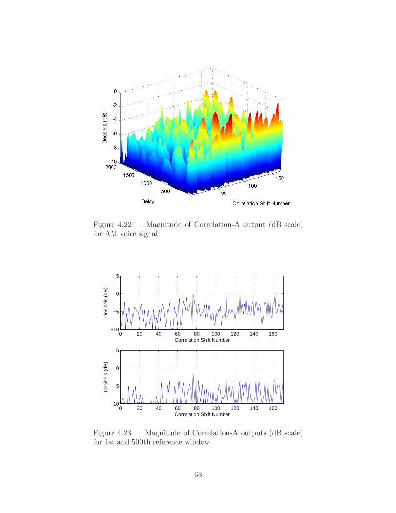
Figure 4.22: Magnitude of Correlation-A output (dB scale)for AM voice signal

0 20 40 60 80 100 120 140 160−10

−5

0

5


Dec

ibel

s (d

B)

0 20 40 60 80 100 120 140 160−10

−5

0

5


Dec

ibel

s (d

B)


63

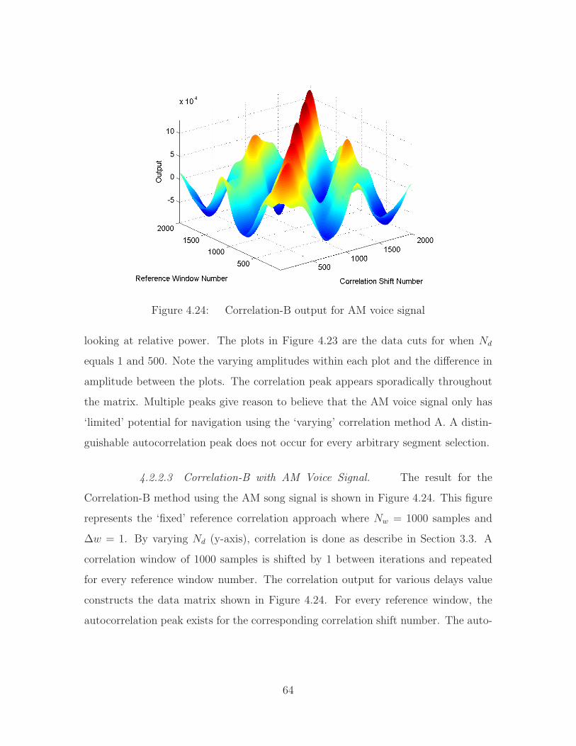
Figure 4.24: Correlation-B output for AM voice signal



amplitude between the plots. The correlation peak appears sporadically throughout

the matrix. Multiple peaks give reason to believe that the AM voice signal only has

‘limited’ potential for navigation using the ‘varying’ correlation method A. A distin-

guishable autocorrelation peak does not occur for every arbitrary segment selection.

4.2.2.3 Correlation-B with AM Voice Signal. The result for the

Correlation-B method using the AM song signal is shown in Figure 4.24. This figure

represents the ‘fixed’ reference correlation approach where Nw = 1000 samples and

∆w = 1. By varying Nd (y-axis), correlation is done as describe in Section 3.3. A

correlation window of 1000 samples is shifted by 1 between iterations and repeated

for every reference window number. The correlation output for various delays value

constructs the data matrix shown in Figure 4.24. For every reference window, the

autocorrelation peak exists for the corresponding correlation shift number. The auto-

64

Figure 4.25: Magnitude of Correlation-B output (dB scale)for AM voice signal

0 500 1000 1500 2000−10

−8

−6

−4

−2

0

2


Dec

ibel

s (d

B)

0 500 1000 1500 2000−10

−8

−6

−4

−2

0

2


Dec

ibel

s (d

B)


65

correlation peak is expected to be seen on the diagonal of the data matrix. However

there are other peaks not on the diagonal that are relatively close in amplitude.




equals 1330 and 249. These reference window numbers were selected as the largest

and smallest autocorrelation peak. Note the varying amplitudes within each plot

and the difference in amplitude between the plots. In terms of potential navigation,

there are too many peaks within 2.0 dB of each other making it difficult to identify

the actual autocorrelation peak. This undistinguishable result gives reason to believe

that the AM voice signal only has ‘limited’ potential for navigation using the ‘fixed’

correlation method B. One distinguishable autocorrelation peak does not occur for

every arbitrary segment selection.

4.3 FM Radio Signal

The results shown in this section are for the FM radio signal. The results are

organized by frontend results, Correlation-A results with song and voice signals, and

Correlation-B results with song and voice signals. The frontend results are shown to

verify that the signal out of the BB filter is the desired signal. The correlation results

are shown by varying the signal delay. The results for the correlation process are

organized into three plots. The first plot is the raw correlation data. The second plot

is the normalized-dB scaled correlation data. And the last plot takes the cuts from

the largest and smallest autocorrelation peak of the normalized-dB scaled data. The

results are repeated for each correlation method and each signal data type.

4.3.1 FM Song Signal Results and Analysis. There are two types of data


results deal with the FM song signal as the input to the system model.

66

2.43 2.432 2.434 2.436 2.438 2.44

−1

0

1

Time (Sec)

Am

plitu

de

2.43 2.432 2.434 2.436 2.438 2.44

−0.5

0

0.5

Time (Sec)

Am

plitu

de

Figure 4.27: Conditioned FM song signal - Received (top) andDown-Converted (bottom) signal

4.3.1.1 Frontend Process Results for FM Song Results. Figure 4.27


is the received FM song signal where the bottom plot is the down-converted output




4.3.1.2 Correlation-A with FM Song Signal. The result for the Correlation-

A method using the FM song signal when varying Nd is shown in Figure 4.28. This

figure represents the ‘varying’ reference correlation approach where Nw = 1000 sam-

ples and ∆w = 1000. The ∆w is set to 1000 samples to simulate a real-time process.

By varying Nd (y-axis), correlation is done as describe in Section 3.3. The correla-

tion window of 1000 samples is shifted by 1000 between iterations and repeated for

all the delay values. The correlation output for various delays values constructs the

data matrix shown in Figure 4.28. The max peaks are suppose to represent the au-

tocorrelation value. This plot does have distinguished max peaks but the results are

67

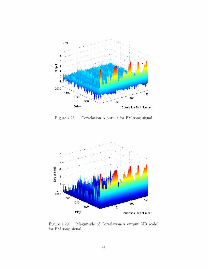
Figure 4.28: Correlation-A output for FM song signal

Figure 4.29: Magnitude of Correlation-A output (dB scale)for FM song signal

68

0 20 40 60 80 100 120 140 160−15

−10

−5

0

5


Dec

ibel

s (d

B)

0 20 40 60 80 100 120 140 160−15

−10

−5

0

5


Dec

ibel

s (d

B)


somewhat inconsistent across the correlation shift number. This results means that

there is not a guarantee of good CPI for any arbitrary segment of the signal.





amplitude between the plots. The correlation peak appearing only when Nd = 0. And

when Nd = 0, the magnitude of the autocorrelation peak varies and is now dependent

on the correlation shift number. This gives reason to believe that the FM song signal

only has ‘limited’ potential for navigation using the ‘varying’ correlation method A.

A distinguishable autocorrelation peak does not occur for every arbitrary segment

selection.

4.3.1.3 Correlation-B with FM Song Signal. The result for the Correlation-

B method using the FM song signal is shown in Figure 4.31. This figure represents

69

Figure 4.31: Correlation-B output for FM song signal

Figure 4.32: Magnitude of Correlation-B output (dB scale)for FM song signal

70

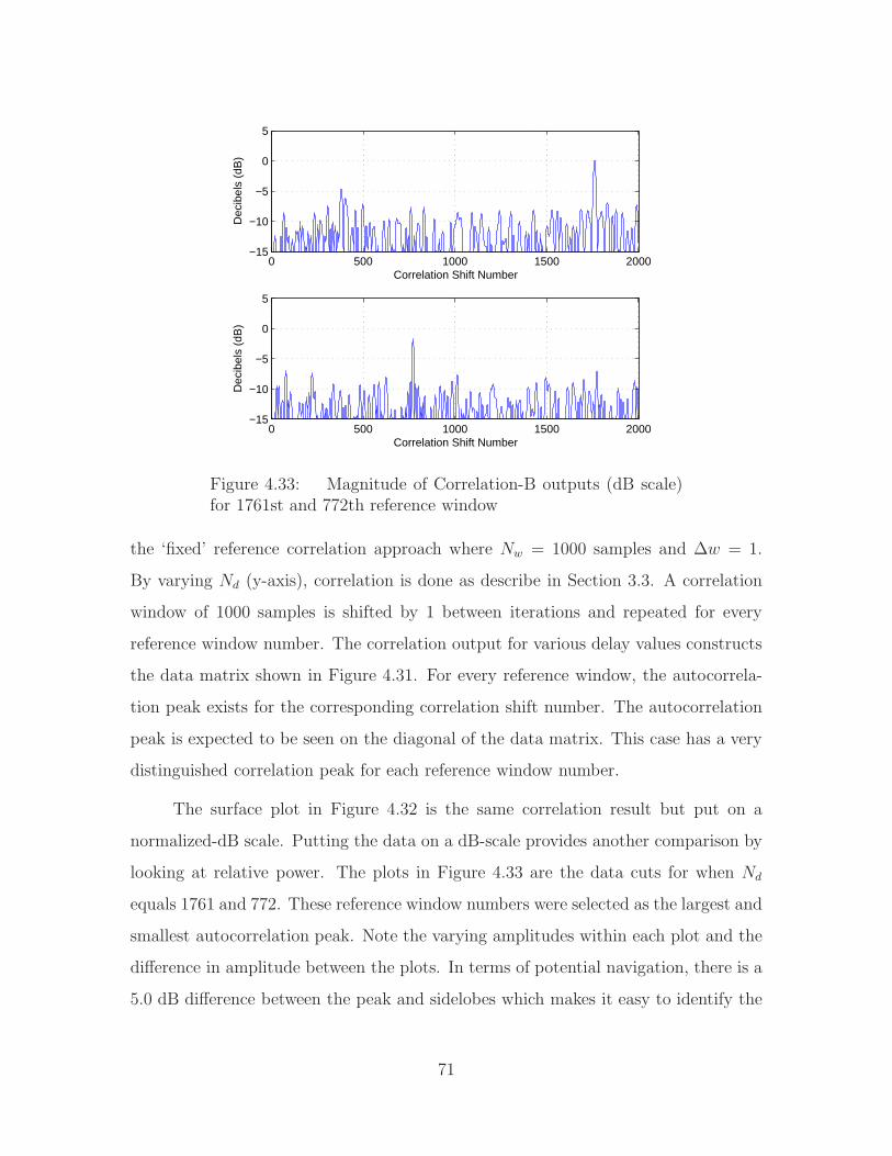
0 500 1000 1500 2000−15

−10

−5

0

5


Dec

ibel

s (d

B)

0 500 1000 1500 2000−15

−10

−5

0

5


Dec

ibel

s (d

B)

Figure 4.33: Magnitude of Correlation-B outputs (dB scale)for 1761st and 772th reference window

the ‘fixed’ reference correlation approach where Nw = 1000 samples and ∆w = 1.

By varying Nd (y-axis), correlation is done as describe in Section 3.3. A correlation

window of 1000 samples is shifted by 1 between iterations and repeated for every

reference window number. The correlation output for various delay values constructs

the data matrix shown in Figure 4.31. For every reference window, the autocorrela-

tion peak exists for the corresponding correlation shift number. The autocorrelation

peak is expected to be seen on the diagonal of the data matrix. This case has a very

distinguished correlation peak for each reference window number.




equals 1761 and 772. These reference window numbers were selected as the largest and

smallest autocorrelation peak. Note the varying amplitudes within each plot and the

difference in amplitude between the plots. In terms of potential navigation, there is a

5.0 dB difference between the peak and sidelobes which makes it easy to identify the

71

2.43 2.432 2.434 2.436 2.438 2.44

−1

0

1

Time (Sec)

Am

plitu

de

2.43 2.432 2.434 2.436 2.438 2.44−0.1

−0.05

0

0.05

0.1

Time (Sec)

Am

plitu

de

Figure 4.34: Conditioned FM voice signal - Received (top)and Down-Converted (bottom) signal

autocorrelation peak. This definite result gives reason to believe that the FM song

signal has ‘promising’ potential for navigation using the ‘fixed’ correlation method

B. Every autocorrelation peak is distinguishable and independent of the reference

window number (i.e., arbitrary segment selection).

4.3.2 FM Voice Signal Results and Analysis. There are two types of data


results deal with the FM voice signal as the input to the system model.

4.3.2.1 Frontend Process Results for FM Voice Results. Figure 4.34


is the received FM voice signal where the bottom plot is the down-converted output




72

Figure 4.35: Correlation-A output for FM voice signal

Figure 4.36: Magnitude of Correlation-A output (dB scale)for FM voice signal

73

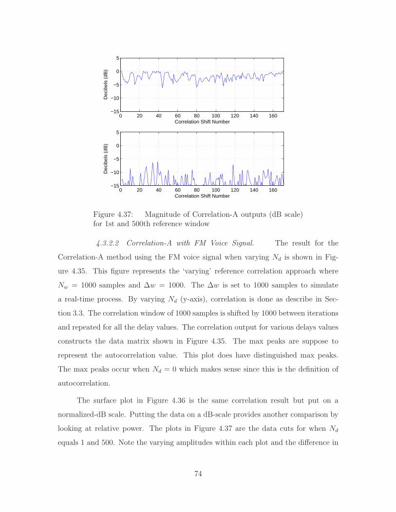
0 20 40 60 80 100 120 140 160−15

−10

−5

0

5


Dec

ibel

s (d

B)

0 20 40 60 80 100 120 140 160−15

−10

−5

0

5


Dec

ibel

s (d

B)


4.3.2.2 Correlation-A with FM Voice Signal. The result for the

Correlation-A method using the FM voice signal when varying Nd is shown in Fig-

ure 4.35. This figure represents the ‘varying’ reference correlation approach where

Nw = 1000 samples and ∆w = 1000. The ∆w is set to 1000 samples to simulate

a real-time process. By varying Nd (y-axis), correlation is done as describe in Sec-

tion 3.3. The correlation window of 1000 samples is shifted by 1000 between iterations

and repeated for all the delay values. The correlation output for various delays values

constructs the data matrix shown in Figure 4.35. The max peaks are suppose to

represent the autocorrelation value. This plot does have distinguished max peaks.

The max peaks occur when Nd = 0 which makes sense since this is the definition of

autocorrelation.





74

Figure 4.38: Correlation-B output for FM voice signal

amplitude between the plots. The correlation peak appearing only when Nd = 0. And

when Nd = 0, the magnitude of the autocorrelation peak varies and is now dependent

on the correlation shift number. This gives reason to believe that the FM voice signal

only has ‘limited’ potential for navigation using the ‘varying’ correlation method A.

A distinguishable autocorrelation peak does not occur for every arbitrary segment

selection.

4.3.2.3 Correlation-B with FM Voice Signal. The result for the

Correlation-B method using the FM song signal is shown in Figure 4.38. This figure

represents the ‘fixed’ reference correlation approach where Nw = 1000 samples and

∆w = 1. By varying Nd (y-axis), correlation is done as describe in Section 3.3. A

correlation window of 1000 samples is shifted by 1 between iterations and repeated

for every reference window number. The correlation output for various delays values

constructs the data matrix shown in Figure 4.38. For every reference window, the

autocorrelation peak exists for the corresponding correlation shift number. The au-

75

Figure 4.39: Magnitude of Correlation-B output (dB scale)for FM voice signal

0 500 1000 1500 2000−15

−10

−5

0

5


Dec

ibel

s (d

B)

0 500 1000 1500 2000−15

−10

−5

0

5


Dec

ibel

s (d

B)

Figure 4.40: Magnitude of Correlation-B outputs (dB scale)for 169st and 1846th reference window

76

tocorrelation peak is expected to be seen on the diagonal of the data matrix. This

case has a very distinguished correlation peak for each reference window number.




equals 169 and 1846. These reference window numbers were selected as the largest

and smallest autocorrelation peak. Note the varying amplitudes within each plot

and the difference in amplitude between the plots. In terms of potential navigation,

there is at least a 5.0 dB difference between the peak and sidelobes which makes it

easy to identify the autocorrelation peak. This positive result gives reason to believe

that the FM song signal has ‘promising’ potential for navigation using the ‘fixed’

correlation method B. Every autocorrelation peak is distinguishable and independent

of the reference window number (i.e., arbitrary segment selection).

4.4 Summary

This chapter presented and analyzed results from simulations conducted with

the receiver model and two correlation methods. The system model was validated by

presenting and analyzing the simulation results for the 31-Gold Code RBW signal.

The AM radio signals were used in the simulations, with all AM radio results showing

‘limited’ potential for navigation. However, the FM radio signals provided ‘promising’

results for both the voice and song data files considered. Only the correlation method

B with both FM radio signals produced distinct autocorrelation peaks for all reference

window numbers. The correlation peaks occur regardless of which window is used as

a reference means that TDOA can be done with FM radio signals using the ‘fixed’

correlation method B. Using one reference receiver and two target receivers, TDOA

can be used on the FM radio signal Correlation-B peaks to navigate. The FM radio

signals showed ‘limited’ potential when using the ‘varying’ correlation method A.

77

V. Conclusions and Recommendations

This chapter summarizes the research results of the correlation receiver model

and CPI/navigation potential of AM and FM radio signals. Recommendations

for future research using AM and FM radio signals, as well as other signals, are also

provided.

5.1 Summary of Results

The primary objective of this research was to determine the CPI of arbitrary

AM and FM radio signals for the purpose of navigation. In support of this objective,

this research investigated two separate correlation receiver methods can hopefully be

used to produce desired autocorrelation peaks between the received signals of the

reference and target receivers. This section summarizes the test results presented in

Chapter IV.

5.1.1 Correlation Receiver Model Results. Two of three components of the

correlation receiver (Figure 3.2) were modelled and performance simulated under this

research. The components considered were the RF-IF frontend and the correlation

processing. The RF-IF frontend process performed as it was designed. It effectively

filters out unwanted noise and brought the input signal down to baseband frequency

as seen in Figure 4.1 and Figure 4.2.

Two correlation methods were designed so that any generic signal can be ana-

lyzed as the input signal and not just the AM and FM radio signals considered here.

Models for the two correlation methods were analyzed and verified by using an input

signal having well-defined and known correlation characteristics. Using a well-known

31-Gold coded signal as the input signal, it was verified/validated that both corre-

lation models performed as designed. For ease of presentation and discussion, one

correlation technique is called Correlation A and produces results which are repre-

sentative of a ‘varying’ reference correlator. The other correlation technique is called

78

Correlation B and produces results which are representative of a ‘fixed’ reference

correlator.

• Correlation Methods - Varying Sample Delay Value (Nd)

Correlation A shows trackable autocorrelation peaks for periodic signals re-

gardless of the correlation shift number. The peaks appear for delay values

corresponding to multiples of the signal period. Figure 4.3 shows this result.

Every autocorrelation peak is distinguishable and independent of the correlation

shift number (i.e., arbitrary segment selection). Therefore, ‘promising’ potential

when periodic signals are used.

Correlation B shows trackable autocorrelation peaks for periodic signals regard-

less of which correlation window is selected. The peaks appear for all correlation

shift numbers corresponding to a respective delay value (i.e., reference window

number). The peaks also occur every signal period. Figure 4.7 shows this result.

Every autocorrelation peak is distinguishable and independent of the reference

window number (i.e., arbitrary segment selection). Therefore, ‘promising’ po-

tential when periodic signals are used.

• Correlation Methods - Varying Correlation Window Size (Nw)

Both Correlation A and Correlation B show that the magnitude of the autocor-

relation peak is directly proportional to correlation window size. As the correla-

tion window increases, so does the magnitude of the autocorrelation peak. The

user may use any correlation window size as long as the results are meaningful.

Figure 4.11 and Figure 4.12 show this result.

The simulations for signals other than the reference signal showed the same overall

trend where a larger correlation window yielded larger autocorrelation peak magni-

tudes. Thus, the correlation window size was fixed for all subsequent analysis and

only the correlation delay was varied. For this research, the correlation window sizes

were selected to be large enough to give meaningful results.

79

5.1.2 Correlation Peak Identifiability of AM Radio. Although not 100%

conclusive, analysis of initial results indicate that the navigation potential of AM

radio signals may be limited. These results are based on CPI and arbitrary segment

selection. The variation of results are shown below. The dB-scale surface plots are

the primary tool for making these conclusions.

• AM Song Signal with Correlation-A

The dB-scale surface plot of the AM song signal using Correlation A is shown in

Figure 4.15. The correlation peak only appears sporadically when Nd = 0. At Nd

= 0, the magnitude of the autocorrelation peak varies and is clearly dependent

on the correlation shift number. This inconsistent trend gives reason to believe

that the AM song signal only has ‘limited’ potential for navigation using the

‘varying’ correlation method A. A distinguishable autocorrelation peak does not

occur for every arbitrary segment selection.

• AM Song Signal with Correlation-B

The dB-scale surface plot of the AM song signal using Correlation B is shown

in Figure 4.18. In terms of navigation potential, the actual autocorrelation

peak is difficult to identify because there are many peaks within 2.0 dB of

each other. These relatively indistinguishable results give reason to believe that

the AM song signal only has ‘limited’ potential for navigation using the ‘fixed’

correlation method B. An autocorrelation peak does occur for every arbitrary

segment selection but it is not definitely distinguishable.

• AM Voice Signal with Correlation-A

The dB-scale surface plot of the AM voice signal using Correlation A is shown

in Figure 4.22. The correlation peak appears sporadically throughout the ma-

trix. Multiple peaks give reason to believe that the AM voice signal only has

‘limited’ potential for navigation using the ‘varying’ correlation method A. A

distinguishable autocorrelation peak does not occur for every arbitrary segment

selection.

80

• AM Voice Signal with Correlation-B

The dB-scale surface plot of the AM voice signal using Correlation B is shown

in Figure 4.25. In terms of navigation potential, there are many peaks within

2.0 dB of each other making it difficult to identify the actual autocorrelation

peak. This undistinguishable result gives reason to believe that the AM voice

signal only has ‘limited’ potential for navigation using the ‘fixed’ correlation

method B. One distinguishable autocorrelation peak does not occur for every

arbitrary segment selection.

The CPI for both song and voice AM radio signals for the purpose of navigation has

been shown to be limited when using either correlation method. In the real-world,

AM stations carry mostly spoken programs while FM stations carry mostly music [2].

It would be interesting to see if real AM radio voice signals would have promising

navigation potential using this correlation receiver model.

5.1.3 Correlation Peak Identifiability of FM Radio. The variation with the

most promising navigation potential of FM radio signals are the results with the

‘fixed’ reference Correlation B. These results are based on CPI and arbitrary segment

selection. The variation of results are shown below. The dB-scale surface plots are

the primary tool for making these conclusions.

• FM Song Signal with Correlation A

The dB-scale surface plot of the FM song signal using Correlation A is shown

in Figure 4.29. The correlation peak appearing only when Nd = 0. And when

Nd = 0, the magnitude of the autocorrelation peak varies and is now dependent

on the correlation shift number. This gives reason to believe that the FM song

signal only has ‘limited’ potential for navigation using the ‘varying’ correlation

method A. A distinguishable autocorrelation peak does not occur for every


81

• FM Song Signal with Correlation B

The dB-scale surface plot of the FM song signal using Correlation B is shown

in Figure 4.32. In terms of navigation potential, there is a 5.0 dB difference

between the peak and sidelobes which makes it easy to identify the autocorre-

lation peak. This definite result gives reason to believe that the FM song signal

has ‘promising’ potential for navigation using the ‘fixed’ correlation method B.



• FM Voice Signal with Correlation A

The dB-scale surface plot of the FM voice signal using Correlation A is shown

in Figure 4.36. The correlation peak appearing only when Nd = 0. And when

Nd = 0, the magnitude of the autocorrelation peak varies and is now dependent

on the correlation shift number. This gives reason to believe that the FM voice

signal only has ‘limited’ potential for navigation using the ‘varying’ correlation

method A. A distinguishable autocorrelation peak does not occur for every


• FM Voice Signal with Correlation B

The dB-scale surface plot of the FM voice signal using Correlation B is shown in

Figure 4.39. In terms of navigation potential, there is at least a 5.0 dB difference

between the peak and sidelobes which makes it easy to identify the autocorrela-

tion peak. This positive result gives reason to believe that the FM song signal

has ‘promising’ potential for navigation using the ‘fixed’ correlation method B.



The CPI for both song and voice FM radio signals for the purpose of navigation

is promising when using the ‘fixed’ reference Correlation B. Correlation A seems to

only provide promising navigation potential when the signal is periodic. Unfortu-

nately, AM and FM radio signals generally do not possess periodic structure. In the

82

real-world, FM stations predominantly carry music programs while AM stations pre-

dominantly carry voice programs [2]. It would be interesting to see how the navigation

potential of real FM radio signals depends on voice or song modulation when using

‘fixed’ reference Correlation B.

5.2 Future Work

This research focused exclusively on simulation and there many different oppor-

tunities to expand the research. A few possible areas for future work are recommended

below.

• TDOA Measurements

Due to time constraints, actual TDOA measurements were never taken in this

research. So the next logical step is to develop TDOA algorithms that determine

the accuracy and usefulness of navigating with AM and FM radio signals. A

simulated model would first need to be designed before real data is used.

• Integration with Universal Software Radio Peripheral (USRP)

The Air Force Institute of Technology now has access to the Universal Software

Radio Peripheral (USRP) receiver. The USRP is designed to allow general

purpose computers to function as high bandwidth software radios [6]. The

basic concept is that the USRP can replace the frontend receiver model of this

research and collect real data. The daughter-boards of the USRP act as the

RF frontend while the mother-board performs at the IF or BB level. The next

challenge is to determine what is actually output from the USRP receiver and

determine how the data can be used in the correlator models in this research.

The USRP will hopefully allow the user to collect real filtered-downconverted

data. With this capability, the simulated results of this thesis could be verified,

as well as additional determinations made on the CPI and navigation potential

of real-world AM and FM radio signals.

83

• Different Signal Types

The real-world has so many different types of information being broadcast via

radio signals. Another possible area of work is determining if there is difference

of CPI and navigation potential for different signal types, e.g., signals generated

for different musical genre: jazz, pop, rap, classical, etc. This research looked

briefly into the difference between song and voice but it would be interesting to

see if there is a difference between different genres of music. Related work on

passive radar seems to suggest that a difference will be revealed.

• Different Environments

Ideally, if the user can successfully integrate the USRP receiver with the correlation-

receiver model(s) considered here, it would be interesting to consider additional

experimental variables. Not only could different signal types be used, as stated

above, but the environments where the data is collected could be varied. The

motivation of this research started with GPS not operating well indoors, in ur-

ban areas and in dense vegetation. It would be interesting to analyze data from

these different environments and determine what impact, if any, it has on overall

results.

Again, there are so many different ways to expand upon this research and further

evaluate the CPI and navigation potential of AM and FM radio signals. It is exciting

to think about what may emerge as the correlation receiver techniques considered

herein are integrated with the USRP receiver hardware.

84

Appendix A. MATLAB Code for Correlation Methods

This appendix contains the MatlabR© code used to simulate the two correlation meth-

ods.

Listing A.1: ‘Varying’ Correlation Method A. (appendix1/correlatorA.m)

% Correlator A - ‘Varying ’ Reference

% ‘x’ is the undelayed signal of interest

% ‘Nd ’ is the number of samples for the delay

% ‘Nw ’ is the number of samples in the correlation window

5 % ‘delta_w ’ is the number of samples in the shift

% ‘delta_t ’ is the time increment between samples

% ‘corr_A ’ is the correlation output

function [ corr_A ] = correlatorA(x,Nd,Nw,delta_w ,delta_t)

10

[x_undelay ,x_delay] = delayA(x, Nd);

N = length(x_delay);

prod = x_undelay.*x_delay;

15 lowDex = 1;

highDex = Nw;

i = 1;

corr_A = [];

20 while highDex <= N

corr_A(i) = sum(prod(lowDex:highDex))*delta_t;

lowDex = lowDex + delta_w;

highDex = highDex + delta_w;

25 i = i+1;

end

end

85

Listing A.2: ‘Fixed’ Correlation Method B. (appendix1/correlatorB.m)% Correlator B - ’Fixed ’ Reference

% ‘x’ is the undelayed signal of interest

% ‘Nd ’ is the number of samples for the delay

% ‘Nw ’ is the number of samples in the correlation window

5 % ‘delta_w ’ is the number of samples in the shift

% ‘delta_t ’ is the time increment between samples

% ‘corr_B ’ is the correlation output

function [ corr_B ] = correlatorB(x, Nd , Nw , delta_w , delta_t)

10

[x_undelay ,x_delay] = delayB(x, Nd);

offset = 0;

reference = x_undelay(1+offset:Nw+offset);

15

lowDex = 1;

highDex = Nw;

i = 1;

20

while highDex <= length(x_delay)

shift = x_delay(lowDex:highDex);

corr_B(i) = sum(reference.*shift)*delta_t;

lowDex = lowDex + delta_w;

25 highDex = highDex + delta_w;

i = i+1;

end

end

86

Bibliography

1. Adamy, D. EW 101: A First Course in Electronic Warfare. Artech House,Norwood, Massachusetts, 2001.

2. Centre, B.C. “FM and AM Radio Station Electromagnetic Field Emissions”.Proceedings of the 41st IEEE Vehicular Technology Conference, 1:1–3, June 2003.

3. Cong, Li and Weihua Zhuang. “Hybrid TDOA/AOA Mobile User Location forWideband CDMA Systems”. IEEE Transactions on Wireless Communications,1:439–447, July 2002.

4. Deng, P. and PZ. Fan. “An AOA Assisted AOA Positioning System”. Proceed-ings of the International Conference on Communication Technology, 2:1501–1504,March 2000.

5. Eggert, Ryan J. Evaluating the Navigation Potential of the National TelevisionSystem Committee Broadcast Signal. Thesis, Air Force Institute of Technology,2950 Hobson Way, March 2004.

6. Ettus, Matt. “USRP User’s and Developer’s Guide”. Ettus Research LLC,Febuary 2005. Available at [email protected].

7. Fisher, Kenneth A. Signals to Navigate and Their Exploitation. Ph.D. the-sis, Graduate School of Engineering, Air Force Institute of Technology (AETC),Wright-Patterson AFB OH, December 2002.

8. Garnder, W.A. “Spectral Correlation of Modulated Signals, Part 1: AnalogModulation”. IEEE Transactions, 584–594, November 1987.

9. Goebel, Greg. “Radio Navigation Systems”. Vector Site, Febuary 2005. Availableat http://www.vectorsite.net/ttwiza.html.

10. Kim, Bryan S. Trilateration and Time Difference of Arrival. Research, Air ForceInstitute of Technology, 2950 Hobson Way, June 2005.

11. Lewis, T.S. Radio and Television Engineers’ Reference Book. George NewnesLimited, London, 1955.

12. Lewis, T.S. Empire of the Air: The Men Who Made Radio. HarperCollins, NewYork, 1991.

13. Miller, Mikel M. Non-GPS Precision In-Door and Out-Door Navigation. Researchdescription, Air Force Institute of Technology, 2950 Hobson Way, December 2004.

14. Misra, P and P Enge. Global Positioning System: Signals, Measurements, andPerformance. Ganga-Jamuna Press, Massachusetts, 2001.

15. Mitra, Sanjit K. Digital Signal Processing, A Computer Based Approach.McGraw-Hill, Massachusetts, 2001.

87

16. Prasad, Ramjee and Tero Ojanpera. “An Overview of CDMA Evolution TowardWideband CDMA”. IEEE Communications Surveys, 1(1):2–29, July 1998.

17. Salmasi, Allen and Klein S. Gilhousen. “On the System Design Aspects of CDMAApplied to Digital Cellular and Personal Communications Networks”. Proceedingsof the 41st IEEE Vehicular Technology Conference, 1:19–22, May 1991.

18. Sklar, Bernard. Digital Communications. Prentice Hall, New Jersey, 2001.

19. Temple, Michael A. EENG 669: Digital Communications I. Course notes, AirForce Institute of Technology, 2950 Hobson Way, January 2005.

20. Temple, Michael A. EENG 673: Spread Spectrum Communications. Course notes,Air Force Institute of Technology, 2950 Hobson Way, June 2005.

21. Temple, Michael A. Position Estimation using Non-GPS Waveforms. Coursedescription, Air Force Institute of Technology, 2950 Hobson Way, March 2005.

22. Thomas, N.J., D.G.M. Cruickshank, and D.I. Lauernson. “Performance of aTDOA-AOA Hybrid Mobile Location System”. Second International Conferenceon 3G Mobile Communication Technologies, 1:216–220, March 2001.

23. Wikipedia. GEE. Wikimedia Foundation Inc., Florida, 2006.

24. Wikipedia. Loran. Wikimedia Foundation Inc., Florida, 2006.

25. Wikipedia. Lorenz. Wikimedia Foundation Inc., Florida, 2006.

26. Wikipedia. Radiodetermination. Wikimedia Foundation Inc., Florida, 2006.

27. Wikipedia. Radiolocation. Wikimedia Foundation Inc., Florida, 2006.

28. Wikipedia. Radionavigation. Wikimedia Foundation Inc., Florida, 2006.

29. Wikipedia. Trilateration. Wikimedia Foundation Inc., Florida, 2006.

30. Wikipedia. VHF Omnidirectional Range. Wikimedia Foundation Inc., Florida,2006.

31. Zhu, Liangxue and Jinkang Zhu. “A New Model and its Performance for TDOAEstimation”. IEEE Communications Surveys, 1:2750–2753, March 2001.

88

REPORT DOCUMENTATION PAGE Form ApprovedOMB No. 0704–0188

The public reporting burden for this collection of information is estimated to average 1 hour per response, including the time for reviewing instructions, searching existing data sources, gathering andmaintaining the data needed, and completing and reviewing the collection of information. Send comments regarding this burden estimate or any other aspect of this collection of information, includingsuggestions for reducing this burden to Department of Defense, Washington Headquarters Services, Directorate for Information Operations and Reports (0704–0188), 1215 Jefferson Davis Highway,Suite 1204, Arlington, VA 22202–4302. Respondents should be aware that notwithstanding any other provision of law, no person shall be subject to any penalty for failing to comply with a collectionof information if it does not display a currently valid OMB control number. PLEASE DO NOT RETURN YOUR FORM TO THE ABOVE ADDRESS.

1. REPORT DATE (DD–MM–YYYY) 2. REPORT TYPE 3. DATES COVERED (From — To)

4. TITLE AND SUBTITLE 5a. CONTRACT NUMBER

5b. GRANT NUMBER

5c. PROGRAM ELEMENT NUMBER

5d. PROJECT NUMBER

5e. TASK NUMBER

5f. WORK UNIT NUMBER

6. AUTHOR(S)

7. PERFORMING ORGANIZATION NAME(S) AND ADDRESS(ES) 8. PERFORMING ORGANIZATION REPORTNUMBER

9. SPONSORING / MONITORING AGENCY NAME(S) AND ADDRESS(ES) 10. SPONSOR/MONITOR’S ACRONYM(S)

11. SPONSOR/MONITOR’S REPORTNUMBER(S)

12. DISTRIBUTION / AVAILABILITY STATEMENT

13. SUPPLEMENTARY NOTES

14. ABSTRACT

15. SUBJECT TERMS

16. SECURITY CLASSIFICATION OF:

a. REPORT b. ABSTRACT c. THIS PAGE

17. LIMITATION OFABSTRACT

18. NUMBEROFPAGES

19a. NAME OF RESPONSIBLE PERSON

19b. TELEPHONE NUMBER (include area code)

Standard Form 298 (Rev. 8–98)Prescribed by ANSI Std. Z39.18

23–03–2006 Master’s Thesis Sept 2004 — Mar 2006

EVALUATING THE CORRELATION CHARACTERISTICSOF ARBITRARY AM AND FM RADIO SIGNALS


Bryan S. Kim, Second Lieutenant, USAF

Air Force Institute of TechnologyGraduate School of Engineering and Management (AFIT/EN)2950 Hobson WayWPAFB OH 45433-7765

AFIT/GE/ENG/06-28

AFRL/SNRPMikel M. Miller, PhDBldg. 620, NE Delivery Dock2241 Avionics CircleWP AFB, OH 45433-7301 (973) 255-6127 [email protected]

Approval for public release; distribution is unlimited.

The Global Positioning System (GPS) provides position estimates on the Earth at anytime, anywhere and in anyweather. However, to provide robust positioning, GPS requires an unobstructed path to satellite signals. As such, GPSperformance generally degrades or becomes non-existent in environments such as large urban areas. This researchinvestigates and analyzes the correlation characteristics of arbitrary AM and FM radio signals for the purpose ofnavigation. Simulations are conducted with different combinations of correlation methods (‘fixed’ or ‘varying’),modulation types (AM or FM), and signal types (song or voice). Out of the eight different variations considered, onlytwo provided promising results for the purpose of navigation. Both the FM voice and FM song signals exhibit distinctautocorrelation peaks (i.e., 5.0 dB peak-to-sidelobe ratios) using the ‘fixed’ reference correlation method. However,results for both FM signal types revealed limited potential for navigation when using the ‘varying’ reference correlationmethod. All the AM signals considered yielded relatively limited potential for navigation using either correlation method.

correlation characteristics, AM radio, FM radio, navigation, correlation methods

U U U UU 104

Dr. Michael A. Temple, AFIT/ENG

(937) 255–3636, ext 4279

air force institute of technology - defense ...€œtemple-ism” comments. press-on, sir. second, i...

Documents