air force institute of technology - dtic.mil · iv afit/gae/eny/06-j02 abstract the air force...

A WIND TUNNEL INVESTIGATION OF JOINED WING SCISSOR MORPHING

THESIS

CHRISTOPHER DIKE, ENSIGN, USN

AFIT/GAE/ENY/06-J02

DEPARTMENT OF THE AIR FORCE

AIR UNIVERSITY

AIR FORCE INSTITUTE OF TECHNOLOGY Wright-Patterson Air Force Base, Ohio

APPROVED FOR PUBLIC RELEASE; DISTRIBUTION UNLIMITED

The views expressed in this thesis are those of the author and do not reflect the official policy or position of the United States Air Force, Department of Defense, or the United

States Government.

AFIT/GAE/ENY/06-J02


THESIS

Presented to the Faculty

Department of Aeronautics and Astronautics

Graduate School of Engineering and Management

Air Force Institute of Technology

Air University

Air Education and Training Command

In Partial Fulfillment of the Requirements for the

Degree of Master of Science in Aeronautical Engineering

Christopher Dike, BSME

Ensign, USN

June 2006

APPROVED FOR PUBLIC RELEASE; DISTRIBUTION UNLIMITED

AFIT/GAE/ENY/06-J02


Christopher Dike, BSME Ensign, USN

Approved:

____________________________________ _________ Dr. Milton Franke (Chairman) Date

____________________________________ _________ Dr. Mark F. Reeder (Member) Date

____________________________________ _________ Lt Col Eric J. Stephen (Member) Date

iv

AFIT/GAE/ENY/06-J02

Abstract

The Air Force Research Laboratory’s Munitions Directorate has been looking to

extend the range of its small smart bomb. Corneille [6] has conducted tests to determine

the aerodynamic characteristics of joined wings on a missile and determine if joined

wings are more beneficial than a single wing configuration. The concept of retrofitting

wings on the bomb introduced an interesting problem: storage before deployment. This

study conducted steady-state low speed wind tunnel testing of a joined wing

configuration that morphed from a compact configuration for storage to a full extension.

These steady-state tests examine differing sweep angles of the same joined wing

configuration. The lift and drag as well as pitching moments and rolling moments were

determined and analyzed for the effects of morphing.

v

AFIT/GAE/ENY/06-J02

To my mother, father and brother for all their love and support throughout my life.

vi

Acknowledgements

I would like to thank Dr. Franke for the encouragement, direction, and experience

he shared with me. I would also like to thank Dr. Reeder for taking time out of his

schedule to consult with me about data analysis. I would like to express my sincere

gratitude to Dwight Gehring, AFIT/ENY, John Hixenbaugh, AFIT/ENY, and Jay

Anderson, AFIT/ENY, for all of their help in this project. Mr. Gehring and Mr.

Hixenbaugh conducted the set-up, calibration, and operation of the wind tunnel. Mr.

Anderson deserves a vast amount of credit for the set-up and operation of the ENY rapid

prototype machine.

vii

Table of Contents

Page

Abstract............................................................................................................................. iv

List of Figures................................................................................................................... ix

List of Tables .................................................................................................................. xiv

List of Symbols................................................................................................................ xv

I. Introduction .................................................................................................................... 1

Background.................................................................................................................... 1

Current Studies .............................................................................................................. 2

Problem Statement ......................................................................................................... 3

II. Literature Review.......................................................................................................... 5

Overview........................................................................................................................ 5

Weight Reduction and Improved Structural Integrity ................................................... 6

Lift ................................................................................................................................. 9

Drag ............................................................................................................................. 10

Stability & Control....................................................................................................... 11

Morphing Technologies............................................................................................... 11

This Study .................................................................................................................... 14

III. Experimental Equipment ........................................................................................... 15

The Missile Model ....................................................................................................... 15

Wind Tunnel ................................................................................................................ 22

Strain Gage Balance..................................................................................................... 25

Dantec Hot-wire Anemometer..................................................................................... 26

IV. Experimental Procedures........................................................................................... 27

Balance Calibration...................................................................................................... 27

Test Plan ...................................................................................................................... 27

viii

Page

Computation of Parameters ......................................................................................... 30

Lift............................................................................................................................ 30

Drag.......................................................................................................................... 31

Pitching Moment...................................................................................................... 32

Rolling Moment ....................................................................................................... 33

Compressibility Analysis ......................................................................................... 33

Tare .......................................................................................................................... 34

Blockage Correction ................................................................................................ 34

V. Results & Analysis...................................................................................................... 37

Wind Tunnel Blockage Correction .............................................................................. 37

Wing Configuration Comparison................................................................................. 38

VI. Summary.................................................................................................................... 58

Appendix A...................................................................................................................... 59

Appendix B ...................................................................................................................... 92

Bibliography .................................................................................................................. 109

ix

List of Figures

Figure Page Figure 1 No. 1737. Waco ASO (N4W c/n X3103). Photographed at Evergreen Airfield, Washington, August 2002 [20]. .......................................................................................... 1 Figure 2 Compact and full positions of retrofit joined wings............................................. 4 Figure 3 Negative stagger configuration using wing connectors [1]. ................................. 5 Figure 4 Positive stagger configuration with wings connected to each other [21]. ............ 6 Figure 5 Single cantilever wing box versus joined wing structural box [23]. .................... 7 Figure 6 Fuel volume comparison [10]............................................................................... 8 Figure 7 Asymmetrical wing box [14]................................................................................ 8 Figure 8 Theoretic span efficiency factor for joined wings with or without symmetrical winglets [15]. .................................................................................................................... 11 Figure 9 Variable sweep on a general aircraft [13]........................................................... 12 Figure 10 Wing sweep mechanism [13]. .......................................................................... 13 Figure 11 Wright Brothers’ 1899 Wright Kite wing warping design [8]. ........................ 14 Figure 12 Bare missile model in the wind tunnel. ............................................................ 15 Figure 13 Five wing configurations of 30o swept wing morphing from 90o, against the body, to 30o full extension. ............................................................................................... 16 Figure 14 Profile for all the swept wings.......................................................................... 18 Figure 15 This diagram shows the difference between the profile and the chord. ........... 18 Figure 16 The 90o swept wing showing the wing gap of 2 inches. .................................. 19 Figure 17 Top profile of the five wing morphing configurations of the 30o swept wing. 20 Figure 18 Different view of the five wing morphing configurations of the 30o swept wing............................................................................................................................................ 21 Figure 19 Wind tunnel convergence dimensions [11]. ..................................................... 23

x

Page

Figure 20 AFIT 3' x 3’ wind tunnel schematic [11]. ........................................................ 24 Figure 21 Test Section of tunnel from Figure 20 with the tunnel axis as defined by the hot-wire traverse grid. [9] ................................................................................................. 24 Figure 22 Comparison between the 60o swept plastic and aluminum wings.................... 28 Figure 23 Wind axis and body axis forces........................................................................ 31 Figure 24 Diagram of lifting forces on the missile. .......................................................... 33 Figure 25 Shows placement of hotwire anemometer [16]. ............................................... 35 Figure 26 Hotwire test pattern [9]..................................................................................... 36 Figure 27 Hotwire vs. transducer velocity measurements. ............................................... 37 Figure 28 Comparison between Corneille [6] and this study’s results for the 30o joined wing made of aluminum. .................................................................................................. 39 Figure 29 Lift and drag relations of the 60o joined wing, not morphed, aluminum. ........ 40 Figure 30 Comparison of 30o joined wing, plastic and aluminum at 60 mph. ................. 42 Figure 31 Comparison of 30o joined wing, plastic and aluminum at 80 mph. ................. 42 Figure 32 Comparison of 30o joined wing, plastic and aluminum at 100 mph. ............... 43 Figure 33 Comparison of 30o joined wing, plastic and aluminum at 130 mph. ............... 43 Figure 34 Comparison of 30o joined wing, plastic and aluminum at 145 mph. ............... 44 Figure 35 Lift comparison of the morphing wing set at 60 mph. ..................................... 45 Figure 36 Lift comparison of the morphing wing set at 80 mph. ..................................... 46 Figure 37 Lift comparison of the morphing wing set at 100 mph. ................................... 46 Figure 38 Lift comparison of the morphing wing set at 130 mph. ................................... 47 Figure 39 Lift comparison of the morphing wing set at 145 mph. ................................... 47 Figure 40 Drag comparison of the morphing wing set at 60 mph. ................................... 48

xi

Page

Figure 41 Drag comparison of the morphing wing set at 80 mph. ................................... 49 Figure 42 Drag comparison of the morphing wing set at 100 mph. ................................. 49 Figure 43 Drag comparison of the morphing wing set at 130 mph. ................................. 50 Figure 44 Drag comparison of the morphing wing set at 145 mph. ................................. 50 Figure 45 Comparison of 60o joined wing plastic morphed and the aluminum at 60 mph............................................................................................................................................ 52 Figure 46 Comparison between two runs on the 60o plastic morphed wing testing for repetition at 145 mph. ....................................................................................................... 53 Figure 47 Pitching moment comparison of the morphing wing set at 60 mph................. 54 Figure 48 Pitching moment comparison of the morphing wing set at 80 mph................. 55 Figure 49 Pitching moment comparison of the morphing wing set at 100 mph............... 55 Figure 50 Pitching moment comparison of the morphing wing set at 130 mph............... 56 Figure 51 Pitching moment comparison of the morphing wing set at 145 mph............... 56 Figure 52 Rolling Moment versus angle of Attack for 30o swept, plastic joined wing.... 57 Figure 53 Lift and drag relations of the bare missile. ....................................................... 60 Figure 54 Drag relations of the bare missile. .................................................................... 61 Figure 55 Lift and drag Relations of 30o swept single wing located forward of CG, wings on bottom, aluminum. ....................................................................................................... 62 Figure 56 Drag and pitch relations of the 30o swept single wing located forward of the CG, wings on bottom, aluminum...................................................................................... 63 Figure 57 Lift and drag relations of the 30o swept single wing located forward of the CG, wings on bottom, plastic. .................................................................................................. 64 Figure 58 Drag and pitch relations of the 30o swept single wing located forward of the CG, wings on bottom, plastic............................................................................................ 65 Figure 59 Lift and drag relations of 30o swept single wing located aft of CG, wings on top, aluminum. .................................................................................................................. 66

xii

Page

Figure 60 Drag and pitch relations of the 30o swept single wing located aft of CG, wings on top, aluminum. ............................................................................................................. 67 Figure 61 Lift and drag relations of the 30o swept single wing located aft of CG, wings on top, plastic. ........................................................................................................................ 68 Figure 62 Drag and pitch relations of the 30o swept single wing located aft of CG, wings on top, plastic. ................................................................................................................... 69 Figure 63 Lift and drag relations of 30o swept joined wing, aluminum. .......................... 70 Figure 64 Drag and pitch relations of the 30o joined wing, aluminum............................. 71 Figure 65 Lift and drag relations of 30o swept joined wing, plastic. ................................ 72 Figure 66 Drag and pitch relations of the 30o joined wing, plastic................................... 73 Figure 67 Lift and drag relations of the 45o single wing swept forward, plastic. ............. 74 Figure 68 Drag and pitch relations of the 45o single wing swept forward, plastic. .......... 75 Figure 69 Lift and drag relations of the 45o joined wing, plastic. .................................... 76 Figure 70 Drag and pitch relations of the 45o joined wing, plastic................................... 77 Figure 71 Lift and drag relations of the 60o joined wing, plastic. .................................... 78 Figure 72 Drag and pitch relations of the 60o joined wing, plastic................................... 79 Figure 73 Lift and drag relations of the 60o joined wing, plastic. Second Run. ............... 80 Figure 74 Drag and pitch relations of the 60o joined wing, plastic. Second Run. ............ 81 Figure 75 Lift and drag relations of the 60o joined wing, not morphed, aluminum. ........ 82 Figure 76 Drag and pitch relations of the 60o joined wing, not morphed, aluminum. ..... 83 Figure 77 Lift and drag relations of the 75o joined wing, plastic. .................................... 84 Figure 78 Drag and pitch relations of the 75o joined wing, plastic................................... 85 Figure 79 Lift and drag relations of the 90o joined wing, plastic. .................................... 86

xiii

Page

Figure 80 Drag and pitch relations of the 90o joined wing, plastic................................... 87 Figure 81 Comparison of 60o joined wing between plastic morphed and the aluminum at 80 mph. ............................................................................................................................. 88 Figure 82 Comparison of 60o joined wing between plastic morphed and the aluminum at 100 mph. ........................................................................................................................... 88 Figure 83 Comparison of 60o joined wing between plastic morphed and the aluminum at 130 mph. ........................................................................................................................... 89 Figure 84 Comparison of 60o joined wing between plastic morphed and the aluminum at 145 mph. ........................................................................................................................... 89 Figure 85 Comparison between two Runs on the 60o plastic morphed wing testing for repetition at 60 mph. ......................................................................................................... 90 Figure 86 Comparison between two Runs on the 60o plastic morphed wing testing for repetition at 80 mph. ......................................................................................................... 90 Figure 87 Comparison between two Runs on the 60o plastic morphed wing testing for repetition at 100 mph. ....................................................................................................... 91 Figure 88 Comparison between two Runs on the 60o plastic morphed wing testing for repetition at 130 mph. ....................................................................................................... 91 Figure 89 Comparison of L/D vs Alpha for the 30o Joined wing and Single wings at 60 mph. .................................................................................................................................. 92 Figure 90 Comparison of L/D vs Alpha for the 30o Joined wing and Single wings at 80 mph. .................................................................................................................................. 92 Figure 91 Comparison of L/D vs Alpha for the 30o Joined wing and Single wings at 100 mph. .................................................................................................................................. 93 Figure 92 Comparison of L/D vs Alpha for the 30o Joined wing and Single wings at 130 mph. .................................................................................................................................. 93 Figure 93 Comparison of L/D vs Alpha for the 30o Joined wing and Single wings at 145 mph. .................................................................................................................................. 94

xiv

List of Tables Table Page Table 1 Various parameters of the model configurations................................................. 17 Table 2 Fan and motor specifications [11]. ...................................................................... 22 Table 3 Maximum loads of AFIT’s 25 lb balance............................................................ 25 Table 4 Model Test Configurations .................................................................................. 29 Table 5 Difference in velocity between the transducer and hotwire. ............................... 37

xv

List of Symbols

a – Distance from the force N1 to the center of gravity

A – Axial force

AR – Aspect ratio

ARF – Aspect ratio of front wing

ARR – Aspect ratio of rear wing

b – Span; Distance from the force N2 to the center of gravity

c – Chord

CD – Drag coefficient

CDi – Induced drag coefficient

CDo – Incompressible drag coefficient

CG – Center of gravity

CL – Lift coefficient

CLmax – Maximum lift coefficient

CLo – Incompressible lift coefficient

CM,0 – Initial pitching moment coefficient

CM – Pitching moment coefficient

D – Drag

e – Span efficiency factor

h – Maximum distance between joined wings

L – Lift

L’ – Rolling moment

M – Pitching moment

xvi

M∞ - Free stream Mach number

N – Total normal force

N1 – Normal force measured at location 1

N2 – Normal force measured at location 2

Re – Reynolds number

S – Reference area

SF – Area of the front wing

SR – Area of the rear wing

UOT – Free stream velocity, Open tunnel

UTr – Free stream velocity, Transducer (Beginning of tunnel)

V∞ - Free stream velocity

α – Angle of attack

tcε – Total blockage

ΛLE – Sweep angle of the leading edge of the wing

ρ∞ – Free stream density

X – Tunnel axis coordinate

Y – Tunnel axis coordinate

Z – Tunnel axis coordinate

1

A WIND TUNNEL INVESTIGATION OF

JOINED WING SCISSOR MORPHING

I. Introduction

Background

Multiple lifting surfaces provide more lift over the single lifting surface concept.

Early biplanes are a perfect example. The multiple wings gave more lifting surfaces and

thus more lift, but the draw back was more profile drag. This profile drag came from the

struts and wires, which can be seen in Figure 1. These struts and wires give the multiple

wings extra support which would void the lifting benefits gained. The concept of multiple

wings lost favor as structural technology advanced [3].

Figure 1 No. 1737. Waco ASO (N4W c/n X3103). Photographed at Evergreen Airfield, Washington, August 2002 [20].

The lift to drag ratio is a very important ratio in considering the aircraft’s

aerodynamic efficiency. The higher the lift to drag ratio, the farther the aircraft can fly or

2

more weight it can carry for the same amount of fuel used. Structural advancements led

to the single wing cantilever wing being dominantly used in aircraft over the last few

decades. Cantilever wings remove more profile drag than the lift that is lost due to less

lifting surfaces which results in a higher lift to drag ratio.

Due to continuing structural advancement, the idea of multiple wings is

resurfacing. The joined wing idea, specifically, is more structurally sound with less

profile drag and induced drag. With the proper design, the joined wing configuration can

weigh less than its single wing counter part if constrained by same lift to drag ratio [3]. In

addition to the aerodynamic improvements, there are more control surfaces which give

more control to the aircraft.

Current Studies

The concept of multiple wings began resurfacing in the early 1980s with the

studies and patents of Wolkovitch [22]. Many studies are being done by companies such

as Boeing and Lockheed Martin, to put the benefits of the joined wing concept to use.

Boeing has a joined wing design that could replace the Navy’s E-2C Hawkeye. Tests

have been conducted in a LaRC 16 foot transonic wind tunnel [6]. Lockheed Martin has

proposed a new joined wing tanker design with two booms. The purpose is to carry more

fuel per tanker and reduce the amount of tankers needed to refuel aircraft [6]. CFD

programs have also been developed to analyze joined wing designs [15].

The Air Force Research Laboratory (AFRL) Munitions Division would like to

extend the range of smart bombs to allow the delivery aircraft to deploy the missile from

a much safer distance from the enemy defenses [6].

3

The Air Force Institute of Technology (AFIT) has conducted an investigation on a

missile model with joined wings to see if the added benefits would be better than adding

cantilever wings to the missile.

Problem Statement

Tests conducted by Corneille [6] showed that joined wing configurations increase

range by 30% or more. The difficulty with wings on missiles is the carriage ability of the

aircraft that delivers the missile. Wings increase the area required for storage. This is

unacceptable. The wings need to be able to morph, or change shape, to take up less space

in storage. When these missiles are dropped from the delivery aircraft, the wings will

then morph from their compact position against the missile body to their extended

position. One concept that this study will look at is the scissors morph. The scissors

morph maintains the connecting points to the missile rather than having moveable

connection points. This should simplify the design because the morphing will be

contained solely in the wings that are attached. There are four axis points. Two of the axis

points where the wings connect to the missile and two moving axis points that are the

wing connectors, shown in Figure 2. As the wings swing out from the missile body, the

wing connectors will move along the centerline to each of the wing’s wingtips. This

study will look at the effects this morphing, or change in configuration, will have on lift,

drag and stability of the missile.

4

Figure 2 Compact and full positions of retrofit joined wings.

Axis Points on Missile

Moving Axis Point, Wing Connector

5

II. Literature Review

This section reviews previous tests and inspections, one of which is Corneille’s

[6] investigation because this is a direct follow-on to her work.

Overview

Wolkovitch stated that, “the joined-wing airplane may be defined as an airplane

that incorporates tandem wings arranged to form diamond shapes in both plan and front

views” [23]. There are many configurations that will achieve this definition. One

configuration is known as negative stagger. It attaches the front wing forward and low on

the fuselage and swept back. The aft wing is attached back and high on the fuselage. The

wings then can be joined together by having wing connectors, structural components for

rigidity, or by having dihedral on both wings such that they attach directly to each other.

Figure 3 shows this negative stagger configuration with wing connectors.

Figure 3 Negative stagger configuration using wing connectors [1].

6

The wing configuration known as positive stagger switches the forward wing

from the bottom of the fuselage to the top of the fuselage and the aft wing from the top to

the bottom of the fuselage. Figure 4 shows the positive stagger configuration with the

dihedral for them to directly connect to each other without wing connectors.

Figure 4 Positive stagger configuration with wings connected to each other [21].

The joined wing has many claimed advantages over the single wing cantilever

that is currently used for almost every aircraft. Some of these advantages include lighter

weight, higher stiffness, higher CL max, lower drag, and good stability and control [23].

Weight Reduction and Improved Structural Integrity

Studies have shown that the joined wing configurations with the same projected

areas, sweep angles, and taper ratios give large weight savings over their single wing

counterpart [23]. The joined wing configuration can be 65% to 78% lighter in comparison

to the single wing [10, 23].

It is important to note that to achieve this weight savings over the single wing, the

geometric parameters must be properly chosen and the internal wing structure must be

optimized [23]. The wing box must occupy the section of the airfoil between 5% and

75% of the chord [23]. Typically the wing box only extends from 15% to 65% of the

7

chord because of the need for larger skin thickness to increase structural integrity [23].

Figure 5 shows the wing box comparison between the cantilever single wing and the

joined wing.

Figure 5 Single cantilever wing box versus joined wing structural box [23].

The larger wing box for the joined wing configuration is possible because of the

increased structural integrity the box shape gives the wings. This allows for less skin

thickness and thus a larger wing box. A larger wing box and multiple wings also means

more fuel capacity as shown in Figure 6.

8

Figure 6 Fuel volume comparison [10].

The box shape of the wings not only adds rigidity to the structure but also resists

longitudinal and vertical loads [18]. Studies show that the most desired arrangement for a

joined wing box is asymmetric, putting more material in the corners that need it to resist

bending [14]. The asymmetric box is shown in Figure 7.

Figure 7 Asymmetrical wing box [14].

9

The joined wing structure is much more complex than its single wing counter

part. Selberg and Cronin [21] have found that the structural complexity of joined wings

leads to an increased number of natural frequencies that produce modes of vibration

containing an unexplainable variety of behaviors.

Tests have also shown that adding cant and twist to the wings can achieve even

higher aerodynamic efficiencies [3]. Again, any improvements that the joined wing

configurations show are dependent on the proper wing properties being chosen, such at

placement, span, and surface area.

Lift

One of the advantages noted earlier is the higher CL max the joined wing

configuration has at trimmed flight [23]. In the joined wing configuration, the front wing

has a tendency to stall, or reaches its CL max at lower angles of attack than the rear wing

[23]. This condition gives the joined wing very good recovery properties, but it is

undesirable because it doesn’t fully utilize the potential lifting capability of the rear wing.

If the rear wing is not reaching its CL max, it is oversized, meaning excess weight that is

not being utilized [23]. It is ideal to have a joined wing design that the front wing stalls

when the rear wing stalls [23]. While this improves efficiency it also decreases the wetted

area while maintaining the same lifting properties [23]. Decreasing the area can also

extend the range since range is a function of lift and drag [2, 4].

Joined wing configurations allow for variation depending on the mission at hand.

They can maintain the same flying weight as a single wing by lengthening the span or

chord, and still have better lifting properties. The joined wing can also carry heavier loads

than the single wing with the same lifting properties [23].

10

Joined wing configurations induce camber. This is caused by the flow being

curved and varies based upon gap and stagger angles [7, 22, 23]. When the single wing is

compared to the joined wing using the same airfoil, the joined wing has shown premature

flow detachment [22]. Specifically for missiles, variable camber has been recommended

for best performance. The camber needs to be reduced to maintain the highest possible

lift to drag, which will maximize the range [22].

Drag

As mentioned in the Introduction, biplanes had a high profile drag issue due to the

extensive structural wiring. Joined wings actually have lower total drag than single wing

configurations. This is due to the lower induced drag than the single wing counterpart at

equal lift, span, and dynamic pressure [2, 14, 18, 22, 23]. This is true for two reasons.

The first reason is that sweeping wings increase induced drag. Although, swept wings

that have the same aspect ratio as straight wings also have the same induced drag

provided the lift distribution is the same [10, 18, 22, 23]. The second reason is the

Prandtl-Munk biplane theory shows that the span efficiency factor can be greater than

one for biplanes [10, 18, 22, 23]. This theory actually predicts efficiency factors for

joined wings to be much lower than wind tunnel tests have shown [22, 23]. For this

reason, Kuhlman and Ku developed a program, summarized by Figure 8, which

accurately predicts the efficiency factor for joined wings [15]. This is important because

the higher the efficiency factor, the lower the induced drag.

11

Figure 8 Theoretic span efficiency factor for joined wings with or without symmetrical winglets [15].

Stability & Control

Joined wings have four controlling surfaces where the single wing configuration

has only two controlling surfaces. More control surfaces mean more control and

stabilizing surfaces. More control leads to better maneuverability [22]. Joined wings have

good spiral stability and no Dutch roll, but do have some pitch down when at high lift

coefficients [22]. Wolkovitch [23] found that adding strakes reduces this pitch down and

increases the maximum lift coefficient.

Morphing Technologies

Traditionally, when wings change sweep they are considered variable sweep. This

definition generally refers to aircraft that have wings at one sweep for flight at low Mach

numbers and another for Mach numbers near and above one. An example is shown in

Figure 9. The F-14, used for decades by the US Navy, uses this technology. It would use

the low sweep for carrier landing and subsonic cruise, and use the high sweep for

12

supersonic flight [13]. According to Raymer [19], variable sweep has a weight penalty in

that the mission might not be acceptable in comparison to the benefits.

An example of a specific variable wing system mechanism for the XF10F-1 is

shown in Figure 10. The wings translate forward at their base and also pivot in when

increasing the wing sweep [13]. This mechanism was considered trouble free by Kress

[13].

Figure 9 Variable sweep on a general aircraft [13].

13

Figure 10 Wing sweep mechanism [13].

According to Guiler and Huebsch [8], wing morphing is defined as camber

control and can be traced back to the Wright Brothers Wright Kite shown in Figure 11.

This glider used a flexible structure and a special weave to warp correctly when actuator

cables were pulled [8]. Camber control is the ability to change the camber of the wing as

needed for the best wing performance [8].

14

Figure 11 Wright Brothers’ 1899 Wright Kite wing warping design [8].

This Study

Morphing for this study will be defined as wing extension. Camber will remain a

constant. The wings will start in the closed position along the fuselage body, a sweep of

90 degrees, and will morph to the full extension after being dropped. This is different

from variable sweep which has multiple wing positions to optimize the flight conditions

as required during flight. The wings in this study cannot. They only change once, from

the position that meets storage restraints to the fully extended position for flight.

15

III. Experimental Equipment

This section describes the equipment and preparation for this study.

The Missile Model The missile model shown in Figure 12, is made of aluminum, is 28.44 in (0.72 m)

long, and has a projected diameter of 2 in (0.0508 m). The missile has four identical tail

fins, two horizontal and two vertical, to give the missile maneuverability and stability in

flight. The airfoil of the tail is symmetric.

Figure 12 Bare missile model in the wind tunnel.

For this study, there are five sweep variations that are all variations of the 30-

degree swept wing with negative stagger. This particular configuration was chosen

because Corneille [6] found that negative stagger was better than positive stagger and the

30 degrees allowed for a wide range of sweep variations. The 30-degree swept wing

starts at 90 degrees, or against the missiles body, and swings out to the 30 degrees swept

16

point. There were 15o intervals used giving wing configurations at 90, 75, 60, 45, and 30

degrees. Figure 13 shows the five wing configurations of the 30-degree wing morphing

from 90 degrees, against the body, to full extension.

Figure 13 Five wing configurations of 30o swept wing morphing from 90o, against the body, to 30o full extension.

These wings are made of plastic. They were designed in SolidWorks, based upon

the specifications of the aluminum 30-degree swept wing and modified to simulate

morphing. The wings were then made in AFIT’s rapid prototype machine. Table 1 gives

the weight, span, reference area, and aspect ratio for the configurations of this study. The

reference area for the bare missile is the projected area and wing planform area for the

30o 45o 60o 75o 90o

17

winged configurations. The aspect ratios and efficiency factors are calculated using

equations that will be discussed later.

Table 1 Various parameters of the model configurations. Weight Span Reference

Area Aspect Ratio

Bare Model 6.85 lbm (3.11 kg)

N/A N/A N/A

30◦ Swept Joined Wing Aluminum

7.62 lbm (3.46 kg)

15.588 in (0.396 m)

0.265 ft2 (0.0246 m2)

7.79

30◦ Swept Joined Wing Plastic

7.2 lbm (3.266 kg)

15.588 in (0.396 m)

0.265 ft2 (0.0246 m2)

7.79


7.2 lbm (3.266 kg)

13.44 in (0.341m)

0.265 ft2 (0.0246 m2)

6.72

60◦ Swept Joined Wing Aluminum

7.67 lbm (3.48 kg)

10.6 in (0.8833 m)

0.265 ft2 (0.0246 m2)

4.50


7.2 lbm (3.266 kg)

10.6 in (0.8833 m)

0.265 ft2 (0.0246 m2)

4.50


7.2 lbm (3.266 kg)

7.10 in (0.5917 m)

0.265 ft2 (0.0246 m2)

3.55


7.2 lbm (3.266 kg)

3.18 in (0.265 m)

0.265 ft2 (0.0246 m2)

1.59

30◦ Swept Single Wing Aluminum

7.12 lbm (3.23 kg)

15.588 in (0.396 m)

0.133 ft2

(0.012 m2) 12.69

30◦ Swept Single Wing Plastic

6.99 lbm (3.17 kg)

15.588 in (0.396 m)

0.133 ft2 (0.012 m2)

12.69

The airfoil profile is shown in Figure 14 where the length is 1 in (0.0254 m) for

all wings. There is no twist or dihedral for any of these wings and there is a wing gap

between the joined wings of 2 in (0.0508 m), the diameter of the missile. The wing gap is

shown in Figure 16. The chord length of all the wings is 1.375 in (0.034925 m). This is

different from the length of the profile because the profile is not parallel to the missile

where the chord length is parallel shown in Figure 15. This airfoil has positive camber,

which consequently causes a negative CM,0 that is not desirable [17]. Because the

18

aerodynamics of a positive camber wing is desirable, a tail is usually required to make

CM,0 positive [17].

Figure 14 Profile for all the swept wings.

Figure 15 This diagram shows the difference between the profile and the chord.

0.5 in.

1 in. 0.25 in.

R0.125 in.

Leading Edge Trailing

Edge

Chord Length

Profile Length

Camber

Leading Edge

Trailing Edge

Leading Edge

Trailing Edge

Forward direction of missile

19

Figure 16 The 90o swept wing showing the wing gap of 2 inches.

The wing connectors are mounted parallel to the missile, i.e. chord length of the

wing. Originally, there were two types of wing connectors tested: curved and straight.

Corneille [6] found no distinct difference between the effects of either. For this study,

only the straight connector was used to reduce the variables. The wing connector is also a

moving body in this study. The wing connector moves towards the wingtips as the wings

morph to their full extension, as seen in Figure 17 and Figure 18. Also notice how the

wing tips are changing between sweeps.

2 in.

20

Figure 17 Top profile of the five wing morphing configurations of the 30o swept wing.

30o 45o

60o 75o

90o

Wing Connectors

Distance Between Roots 9 in. 9 in.

9 in.

9 in. 9 in.

Span

Span

Span

Span

Span


21

Figure 18 Different view of the five wing morphing configurations of the 30o swept wing.

30o 45o

60o 75o

90o

30o 45o

60o 75o

90o


22

Wind Tunnel Experiments were conducted in the AFIT 3’x3’ subsonic wind tunnel, built by the

New York Blower Company. The wind tunnel fan is an ACF/PLR Class IV with a

Toshiba Premium Efficiency (EQP III) fan motor. The fan and the motor are both

controlled by a Siemens (13710) Adjustable Frequency Tunnel Controller. Table 2 shows

the specifications.

Table 2 Fan and motor specifications [11]. Controller Motor

3 phase induction

1785 RPM operating speed

Maximum theoretical speed – 150 mph

Maximum tested speed – 148 mph

250 max HP 200 brake horsepower

460 volts 230/460 volts

315 amps 444/222 amps

60 Hz

4 poles

The tunnel is an open circuit configuration with a closed test section. The fan is

located at the end of the tunnel and pulls the ambient air from the room through a 122”w

x 111”h x 70”l intake plenum. To give the tunnel good laminar streamlines, the plenum

consists of four steel mesh anti-turbulent screens with 1/4" aluminum honeycomb flow-

straightener which has a minimum aspect ratio of 15. The flow travels to the test section

23

through a 95.5” long convergent duct with a contraction ratio of 9:5:1. The height of the

tunnel contracts from the anti-turbulent screen at 111” to the test section of height 31.5”.

Figure 19 displays the wind tunnel convergence dimensions. Figure 20 displays the

schematic of AFIT’s wind tunnel.

Figure 19 Wind tunnel convergence dimensions [11].

The test section volume is 31”h x 44”w x 72”l with an octagonal shape to reduce

corner interference. The test section is shown in Figure 21. The sting mechanism in the

test section is remotely controlled allowing the model to vary the angle of attack from -25

to 25 degrees.

The wind tunnel diverges after the test section and exits the tunnel through a

vertical exhaust pipe. There is a protective fence to protect the fan and motor at the end of

the tunnel from debris, possibly from model failure.

24

Figure 20 AFIT 3' x 3’ wind tunnel schematic [11].

Figure 21 Test Section of tunnel from Figure 20 with the tunnel axis as defined by the hot-wire traverse grid. [9]

CONTROLLER ROOM

+X -X

+Y

-Z

+Z

-Y Wind Exhaust

44 in.

31 in.

Wind Input

72 in.

25

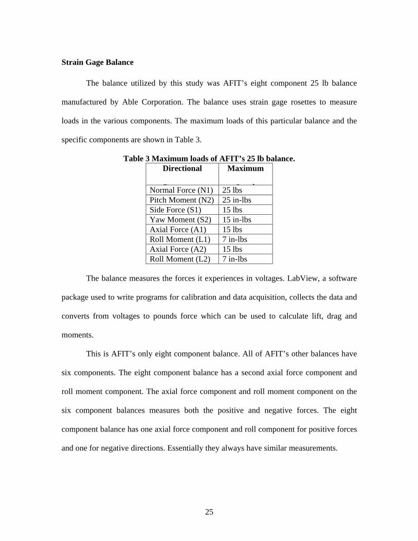
Strain Gage Balance The balance utilized by this study was AFIT’s eight component 25 lb balance

manufactured by Able Corporation. The balance uses strain gage rosettes to measure

loads in the various components. The maximum loads of this particular balance and the

specific components are shown in Table 3.

Table 3 Maximum loads of AFIT’s 25 lb balance. Directional

C t

Maximum

L dNormal Force (N1) 25 lbs Pitch Moment (N2) 25 in-lbs Side Force (S1) 15 lbs Yaw Moment (S2) 15 in-lbs Axial Force (A1) 15 lbs Roll Moment (L1) 7 in-lbs Axial Force (A2) 15 lbs Roll Moment (L2) 7 in-lbs

The balance measures the forces it experiences in voltages. LabView, a software

package used to write programs for calibration and data acquisition, collects the data and

converts from voltages to pounds force which can be used to calculate lift, drag and

moments.

This is AFIT’s only eight component balance. All of AFIT’s other balances have

six components. The eight component balance has a second axial force component and

roll moment component. The axial force component and roll moment component on the

six component balances measures both the positive and negative forces. The eight

component balance has one axial force component and roll component for positive forces

and one for negative directions. Essentially they always have similar measurements.

26

Dantec Hot-wire Anemometer The Streamline 90N10 Constant Temperature Anemometer by Dantec Dynamics

has a tri-axial probe that measures velocities on three coordinate axes. It mounts on a

mechanical arm that extends vertically into the wind tunnel from the top. The mechanical

arm is fully motorized and programmable to transverse in all three axes. A data

acquisition program named Streamware, collects processes and formats the data.

27

IV. Experimental Procedures

This section describes the procedures associated with wind tunnel data collection.

Balance Calibration

The balance was calibrated by applying weights in the six degrees of freedom.

The normal forces were calibrated to 25 lbs (111.2 N), side forces to 15 lbs (66.72 N),

axial forces to 15 lbs (66.72 N), and roll moments to 7.5 in-lbs (0.847 N-m). The weights

being applied to the balance indicated the accuracy of the balance and the interactions, or

forces indicated, in the other degrees of freedom. This information was then used to

correct the balance data read by applying to MatLab data reduction which will be

discussed later.

Test Plan

Low speed wind tunnel tests were conducted on thirteen wing configurations on

the missile model. The different plastic configurations are variations of the original

aluminum 30-degree swept joined wing. The different sweeps are to simulate wing

morphing from compact 90 degrees against the body out to the final extension of 30

degrees. These tests are to show steady state effects of the wings in 15 degree increments.

The test configurations are shown in Table 4. The wing connectors for each wing

simulate moving outboard on each wing configuration as if they are moveable axis

points. This is shown in Figure 17 and Figure 18.

The 60-degree swept aluminum wing and plastic wing were also compared

because of their different configurations. The aluminum configuration has the wing

connectors at the wingtips, where the plastic wing has the wing connectors farther

inboard, closer to the missile. The wingtips are also different in that the plastic wingtip is

28

not parallel to the missile body. This is because it is the 30-degree wing morphed to 60

degrees. The points where the wings are attached to the missiles are also different. These

connection points are closer for the plastic wings. The two wings are compared in Figure

22.

Figure 22 Comparison between the 60o swept plastic and aluminum wings.

Corneille [6] conducted tests at 100 mph (44.7 m/s), 130 mph (58.1 m/s), and 145

mph (64.82 m/s). For comparison purposes, tests in this investigation were run at the

same speeds; however two tests speeds were added, 60 mph (26.82 m/s) and 80 mph

(35.76 m/s). There was an unexplained loss of lift in one of the conducted tests so the

extra speeds were added to show that this was an isolated discrepancy and repeatability

does exist among different speeds.

Aluminum Plastic

29

Each test was conducted at angles of attack of -4 degrees to 15 degrees. The angle

of attack was increased in two degree increments up to 14 degrees then 1 degree for the

final increment. This was also done to compare with Corneille [6].

Table 4 Model Test Configurations Bare Model

30◦ Sweep Aluminum

Single Top Swept forward

Single Bottom Swept aft

Joined Wing

30◦ Sweep Plastic


Single Bottom Swept aft

Joined Wing

45◦ Sweep Plastic (Morphed)


Joined Wing

60◦ Sweep Aluminum

Joined Wing

Plastic (Morphed)

Joined Wing


Joined Wing


Joined Wing

30

Computation of Parameters

The forces measured by the balance are body axis forces. This axis changes with

the orientation of the missile’s body. These forces must be converted to the wind axis, or

the tunnel axis, to calculate the lift and drag forces and the pitching and rolling moments.

The lift, drag, pitching moment and rolling moment coefficients were determined

for each configuration.

Lift

Lift is the component of force normal to the wind axis shown in Figure 23. The

balance reads the normal force and axial force of the missile which must be converted to

the wind axis to get lift, L, using Equation (1), where N is the total normal force, A is the

total axial force, and α is the angle of attack.

L = N cos α – A sin α (1)

Once the lifting force is determined it must be non-dimensionalized, because this

is a scale model. To non-dimensionalize a force, the wing area and dynamic pressure are

divided out of the force. The lift coefficient is the non-dimensional term desired.

Equation (2) calculates the lift coefficient, CL. Reference areas are given in Table 1.

SVLCL 2

21

∞∞

=ρ

(2)

31

Figure 23 Wind axis and body axis forces.

Drag

Drag is the force parallel to the wind axis shown in Figure 23. Again the forces

measured by the balance need to be converted from the body axis to the wind axis.

Equation (3) calculates drag, where N is the total normal force, A is the total axial force

and α is the angle of attack.

D = N sin α + A cos α (3)

Once the drag is calculated from measured values it also was non-dimesionalized

using Equation (4).

SVDCD 2

21

∞∞

=ρ

(4)

This drag coefficient is the sum of profile drag and induced drag. The profile drag

is usually obtained from experimental data. Induced drag is a by-product of lift. Equation

(5) gives the induced drag coefficient, where AR is the aspect ratio, and e is the

efficiency factor. The efficiency factor can be solved for using Figure 8.

eARC

C LID π=, (5)

x

z

Wind Direction

LN

D

A

Angle of Attack, α

Tunnel Axis

32

Normally, the aspect ratio is defined by Equation (6), where b is span and S is

reference area, and this is still true for the single wing configurations. For the joined wing

configurations aspect ratio is redefined by Equation (7), where ART is the total aspect

ratio, ARF is the front wing aspect ratio, SF is the front wing surface area, ARR is the rear

wing aspect ratio, and SR is the rear wing surface area [2]. Equation (7) was used to

calculate the aspect ratio in Table 1.

SbAR

2

= (6)

⎟⎟⎠

⎞⎜⎜⎝

⎛+⎟⎟

⎠

⎞⎜⎜⎝

⎛+

⎟⎟⎠

⎞⎜⎜⎝

⎛+⎟⎟

⎠

⎞⎜⎜⎝

⎛

=11

F

R

R

F

F

RR

R

FF

T

SS

SS

SSAR

SSAR

AR (7)

Pitching Moment

Moments show the stability of an aircraft. The pitching moment is calculated

about the center of gravity of the model by doing a sum of moments. Figure 24 shows the

lifting forces seen by the missile. The balance reads the total lifting forces at the point of

the balance, or N. The pitching moment found by calculating the distance from the center

of gravity to where the balance measures the normal forces as seen in Equation (8), where

a is the distance from center of gravity of the model to the balance strain gage.

M = N a (8)

33

Figure 24 Diagram of lifting forces on the missile.

Then the moment coefficient is determined by applying Equation (9), where c is

the chord length.

ScVMCM 2

21

∞∞

=ρ

(9)

Rolling Moment

The rolling moment shows the tendency for the missile to roll in flight conditions

which would cause control problems. The balance is already on the missile’s rolling axis

and has a component to measure the rolling moment, L’. Equation 10 calculates the

rolling moment coefficient.

ScVLCL 2'

21

'

∞∞

=ρ

(10)

Compressibility Analysis

The maximum speed of the wind tunnel is 145 mph (64.82 m/s), which is well

within the incompressibility regime. This missile is more likely to fly in the

compressibility regime at about Mach 0.7. The Prandtl and Glauert compressibility

Lwing Lwing Ltail

Waircraft=Ltotal=N

X

Z

CG

34

correction Equations (11-12) can give a better idea of the coefficients in the

compressibility region.

2

,

1 ∞−=

M

CC oL

L (11)

2

,

1 ∞−=

M

CC oD

D (12)

These equations are pretty good approximations and can be used up to Mach 0.8

where they can no longer be used due to the anomalies of transonic flow. By simple

analysis of these equations, it should be realized that as Mach increases so will the lift

and drag coefficients.

Tare

When the missile is connected to the balance and there is no flow through the

wind tunnel, the balance still has small readings and needs to be zeroed out like a weight

scale. To do this, the missile is put through a run in the wind tunnel with no wind for each

test configuration. The data measured by the balance for those runs are put into what are

called tare files. Then the model is put through tests at the specified wind speeds, data are

recorded and put into test files. These files are inputted into the MatLab, shown in

Appendix B, which subtracts out the tare data from the test data to give you the actual

force readings of the balance to reduce error.

Blockage Correction

The wind speed at the beginning of the test section, where the pressure transducer

measures the velocity, is different than the point in the tunnel where the model is placed

35

and tested. This is due to friction of the walls of the wind tunnel. This causes the

pressure transducer, which is upstream, to be greater than the point where the model will

be in the test section. The velocity at the model test section is the velocity used for the

aforementioned calculations. Because the transducer is measuring the upstream velocity,

a correction was made to get the velocity at the test section.

The hot-wire anemometer was used to measure the velocity at the point in the test

section where the modes is to be placed. This is an open tunnel measurement. Figure 25

shows how the anemometer was positioned in the tunnel. The hotwire recorded the

velocities at the test location with open tunnel configuration at speeds of 60, 80, 100, 130,

and 145 mph.

Figure 25 Shows placement of hotwire anemometer [16].

14 1/4 “

2”

4 ¾ “

36

The hotwire started measuring the velocity 0.5 mm in the positive Y direction and

was programmed to move in 0.1 mm increments in the pattern shown in Figure 26. The

hotwire measured a 1.0 mm2 plane.

Hot Wire 1mm gridcentered about "sting" CL

-1.2

-1

-0.8

-0.6

-0.4

-0.2

0

0 0.2 0.4 0.6 0.8 1

-y is AWAY from control room

-z is

in U

PWA

RD

S di

rect

io

0

10

20

30

40

50

60

70

80

M/S

sting

Figure 26 Hotwire test pattern [9].

The Dantec Streamware software saves the recorded measurements as voltages.

These measurements are then converted to mph to compare them to the transducer

measurements which are in mph. Equation (13) compares the two velocities, where εtc is

the total blockage, UOT is the freestream velocity at the model or hotwire, and UTr is the

freestream velocity at the beginning of the wind tunnel or transducer.

Tr

OTtc U

U=ε (13)

37

V. Results & Analysis

Using the procedures established in the last chapter, the data were recorded and

analyzed.

Wind Tunnel Blockage Correction

Equation (13) was used to calculate the velocity blockage correction factor

between the hotwire and transducer velocity measurements. Table 5 summarizes the

correction factors for each speed. Figure 27 shows the velocity comparison. These

velocity corrections were then applied to the MatLab code in Appendix B to convert the

recorded velocity of the transducer to the actual velocity the model is experiencing. As

can be seen, the difference between the two ranged from a 4% to 10% difference, which

is normal.

Table 5 Difference in velocity between the transducer and hotwire. 60 mph 80 mph 100 mph 130 mph 145 mph

εtc 0.9111794 0.9002786 0.955283 0.960305 0.954742

0

20

40

60

80

100

120

140

160

60 mph 80 mph 100 mph 130mph 145mph

Win

d Sp

eed

(mph

)

Hotwire

Transducer

Figure 27 Hotwire vs. transducer velocity measurements.

38

Wing Configuration Comparison

All the recorded data were run through the MatLab code in Appendix B, and the

lift, drag, pitch and roll coefficients were calculated. Lift, drag, pitch, and roll curves

were then created to compare the data retrieved.

The first test was conducted to recreate the results from Corneille [6] for the 30-

degree and 60-degree negative stagger, because the tests for this study were conducted in

a different wind tunnel and on a different balance. Figure 28 shows the lift comparison

for the 30-degree swept aluminum joined wings in the new wind tunnel on the 25 lb

balance versus Corneille’s [6] test. To make comparisons, the graph for this study was

transposed on top of Corneille’s [6]. At speeds of 100 mph, 130 mph, and 145 mph the

lift and drag curves are a match to Corneille’s [6] lift coefficient. The same was found for

the 60-degree swept aluminum wings shown in Figure 29, which matches Corneille’s [6]

curve on page 70 of her thesis. This shows that Corneille’s [6] data is consistent and

reproducible, which gives significance to the follow on investigations. Corneille [6]

didn’t test at 60 mph or 80 mph and only tested up to an angle of attack of 13 degrees, so

that data cannot be compared.

It is interesting to note that for all the tests conducted of the 30-degree swept

aluminum joined wing, there are two positions of temporary wing stall. There is one at

about 4 degrees angle of attack and one at about 12 degrees angle of attack. It can also be

noted that for the tests at 60 mph and 80 mph these stall characteristics are seen at lower

angles of attack and more amplified. A similar characteristic is also seen in Hoang and

Soban [10]. It was attributed to a low Reynolds number of 0.4 X 106 and a thin airfoil

selection of 12% of the chord. In this study, the Reynolds number ranged from 0.4 X 106

39

to 1.5 X 106 and the airfoil thickness was 18.25% of the chord. These conditions could be

a possible cause of the wing stall in this study. The wing configuration in Hoang and

Soban [10] was a single wing with 20-degree sweep. Looking at the single wing

configurations with 30-degree sweep from this study in Appendix A, the temporary wing

stall is also seen. It is not solely a condition of just the joined wings in this study. It seems

to be more of a condition of the sweep, specifically the 30-degree sweep in this study.

Wolkovitch [22] also suggests that joined wings have a premature flow detachment

causing wing stall, which could also be a contributor to this study’s wing stall.

-0.5

0

0.5

1

-10 0 10 20

Alpha

C_L

100 mph130 mph145 mph

Figure 28 Comparison between Corneille [6] and this study’s results for the 30o joined wing made of aluminum.

Corneille’s [6] Tests

This Study

Wing Stall

40

-0.5

0

0.5

1

-10 0 10 20

Alpha

C_L

60 mph80 mph100 mph130 mph145 mph

0

0.05

0.1

0.15

0.2

0.25

0.3

0.35

-0.5 0 0.5 1

C_L

C_D


Figure 29 Lift and drag relations of the 60o joined wing, not morphed, aluminum.

41

The next comparison is the plastic versus the aluminum 30-degree swept joined

wing, because it is the main wing of which the morphed wings are derived. The

comparisons at 60, 80, 100, 130, and 145 mph are shown in Figure 30 through Figure 34.

These curve comparisons show that the plastic wings with 30-degree sweep also have the

two losses of lift that the aluminum wings experienced, which was mention earlier. The

major difference is that the plastic wing’s second loss of lift was seen at a lower angle of

attack. This could possibly be due to the difference in stiffness and surface roughness.

The plastic wings are less stiff and rougher than the aluminum configurations.

The 130 mph comparison must be noted because it has the biggest discrepancy at

10 degrees to 13 degrees angle of attack. It was decided to run the tests at 60 mph and 80

mph to see if this discrepancy happened at any other speeds, or if it was a phenomenon of

the 130 mph speed at this specific angle of attack for this particular configuration of

wings. Loss of lift of this magnitude was not seen at any other speeds. The test was then

conducted again with a strobe light to see if the loss of lift is caused by the wing hitting

its resonance frequency. At about 9 degrees angle of attack the wings began to visually

vibrate rapidly until the angle of attack of 13 degrees was reached. The loss of lift can be

attributed to the 30-degree swept plastic joined wings hitting a resonance frequency

causing rapid vibration. Bagwill and Selberg [21] state that the structural complexity of

joined wings increases the number of natural frequencies that produce modes of

vibration. This is the probable cause. The material difference between the plastic and the

aluminum will also add to this effect.

42

-0.5

0

0.5

1

-10 0 10 20

Alpha

C_L 30 deg Plastic

30 deg Aluminum

Figure 30 Comparison of 30o joined wing, plastic and aluminum at 60 mph.

-0.5

0

0.5

1

-10 0 10 20

Alpha

C_L 30 deg Plastic

30 deg Aluminum


43

-0.5

0

0.5

1

-10 0 10 20

Alpha

C_L 30 deg Plastic

30 deg Aluminum


-0.5

0

0.5

1

-10 0 10 20

Alpha

C_L 30 deg Plastic

30 deg Aluminum


44

-0.5

0

0.5

1

-10 0 10 20

Alpha

C_L 30 deg Plastic

30 deg Aluminum


Comparisons were also made between the various degrees of the 30-degree swept

joined wings being morphed/swept back. The results matched expectations given by

Bertin [4], who states that increasing sweep decreases the lift. As the wings are morphed

outward from the missile’s body, the lift coefficient increases until the 45 degree sweep is

reached. Once the wings were morphed to their full extension of 30 degrees, the wings

experienced temporary wing stall at about 2 degrees angle of attack, which brought the

lift coefficient below that of the 45 degree swept wings. This can be seen in Figure 35

through Figure 39. Taking a closer look at these figures, temporary wing stall on the 30-

degree configuration can also be seen on the 45 degree configuration, although it is less

noticeable. This indicates that as the wings open from the 45 degree sweep to the 30-

degree sweep, more wing stall is experienced. This is probably due to the Reynolds

45

number decreasing and becoming too low. The Reynolds number decreases because it is

a function of chord length and as the wings are morphing to their full extension, the chord

length is decreasing. The chord length is the distance from the leading edge of the wing

to the trailing edge and is parallel to the missile’s body. So, as the wing morphs out the

sweep angle and the chord length both decrease.

-0.5

0

0.5

1

1.5

-10 0 10 20

Alpha

C_L

No Wing30 deg45 deg Morphed60 deg Morphed75 deg Morphed90 deg Morphed

Figure 35 Lift comparison of the morphing wing set at 60 mph.

46

-0.5

0

0.5

1

-10 0 10 20

Alpha

C_L



-0.5

0

0.5

1

-10 0 10 20

Alpha

C_L

No Wing30 deg 45 deg Morphed60 deg Morphed75 deg Morphed90 deg Morphed


47

-0.5

0

0.5

1

-10 0 10 20

Alpha

C_L



-0.5

0

0.5

1

-10 0 10 20

Alpha

C_L



48

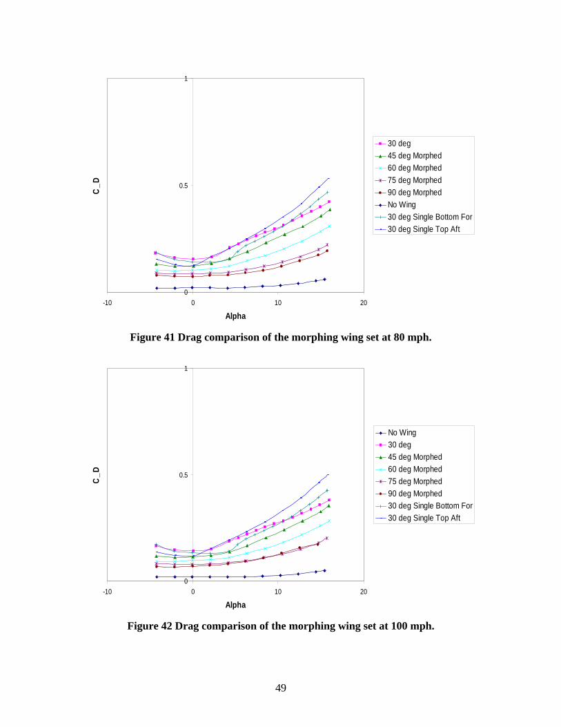
Figure 40 through Figure 44, show that there are drag increases among the wing

configurations as the wings open outward from the body to the fully extended position.

The drag rise is expected because of the increasing frontal area as the wings morph out to

the 30-degree sweep. This is consistent with Bertin [4], who states that increasing sweep

decreases the drag. There is also consistency with the Wolkovitch [22, 23], because both

the 30-degree single wing configurations produce more drag than the 30-degree joined

wing configuration.

0

0.5

1

-10 0 10 20

Alpha

C_D

No Wing30 deg45 deg Morphed60 deg Morphed75 deg Morphed90 deg Morphed30 deg Single Bottom For30 deg Single Top Aft

Figure 40 Drag comparison of the morphing wing set at 60 mph.

49

0

0.5

1

-10 0 10 20

Alpha

C_D

30 deg45 deg Morphed60 deg Morphed75 deg Morphed90 deg MorphedNo Wing30 deg Single Bottom For30 deg Single Top Aft


0

0.5

1

-10 0 10 20

Alpha

C_D

No Wing30 deg 45 deg Morphed60 deg Morphed75 deg Morphed90 deg Morphed30 deg Single Bottom For30 deg Single Top Aft


50

0

0.5

1

-10 0 10 20

Alpha

C_D



0

0.5

1

-10 0 10 20

Alpha

C_D



51

A comparison was made between the morphed 60-degree wing from this study

and the 60-degree aluminum wing from Corneille’s [6] study to see if there are any major

aerodynamic differences. Figure 22 shows the structural differences between the two 60-

degree swept configurations. The major differences are the placement of the wing

connectors, the distance between the wing roots are closer together on the plastic model

than the aluminum configuration, and the wingtips are of different shape. The aluminum

wing’s connectors act as winglets at the wingtips. The plastic configuration has the wing

connectors inboard of the wingtips. Also, the aluminum wing’s wingtips are parallel to

the missile’s body, where the plastic wing’s wingtips are not because they are in a

morphed position from the original 30-degree swept wing. They are parallel when in the

30-degree swept position. A comparison of the aerodynamic properties was done to see

the effects of these differences. The 60 mph comparison is made in Figure 45 which

shows the plastic configuration experiences slightly more lift than the aluminum

configuration. This same result is seen at each of the other test speeds, which can be seen

in Figures 81 to 84 (Appendix A). Winglets have shown to increase the lift-curve slope

and maximum lift coefficient, while decreasing the induced drag [2, 7]. Also tip shape

not parallel to wind flow has shown to decrease lift slope [7]. The results of this test were

inconsistent with all of the literature researched. The wings are too dissimilar, that no

conclusions can be drawn as to what causes the change in lift slope and max lift

coefficient.

52

-0.5

0

0.5

1

-10 0 10 20

Alpha

C_L 60 deg Plastic Morphed

60 deg Aluminum Not Morphed

Figure 45 Comparison of 60o joined wing plastic morphed and the aluminum at 60 mph.

The plastic 60-degree morphed wing configuration was also tested for repetition

to see if the same tests conducted on different days were producing the same results. As

can be seen in Figure 46, the results of the two tests conducted at 145 mph where

identical. This infers that the data taken is reproducible and accurate. Repeatability is also

shown in Appendix A among the runs of different speeds producing similar coefficients

at the same angles of attack.

53

-0.5

0

0.5

1

-10 0 10 20

Alpha

C_L Run 1

Run 2

Figure 46 Comparison between two runs on the 60o plastic morphed wing testing for repetition at 145 mph.

The effects of pitching moment stability were compared among the different wing

configurations at each test speed shown in Figure 47 through Figure 51. As the wings

morph from 90 to 30 degrees, the pitching moment slope becomes less negative, but there

are no major discrepancies to indicate major control issues. It is important to note that

every configuration at every speed, the CM,0 is negative. This is consistent with

Wolkovitch [22, 23], who states that the joined wing configuration induces a positive

camber, which according to Kulhman and Ku [15], causes a negative CM,0. This causes a

stability problem. The missile must either fly with flaps deployed or the horizontal tail

will have to be adjusted to make CM,0 positive for trimmed flight. The tail currently on

the missile is symmetrical in camber which does not affect CM,0 [15]. The same result is

54

also found in the 30-degree swept single wing configurations found in Figures 56, 58, 60,

and 62 (Appendix A), indicating that the joined wings are not solely the cause.

-2.5

-2

-1.5

-1

-0.5

0

0.5

1

-10 0 10 20

Alpha

C_M

30 deg45 deg Morphed60 deg Morphed75 deg Morphed90 deg Morphed

Figure 47 Pitching moment comparison of the morphing wing set at 60 mph.

55

-2.5

-2

-1.5

-1

-0.5

0

0.5

1

-10 0 10 20

Alpha

C_M



-2.5

-2

-1.5

-1

-0.5

0

0.5

1

-10 0 10 20

Alpha

C_M

30 deg 45 deg Morphed60 deg Morphed75 deg Morphed90 deg Morphed


56

-2.5

-2

-1.5

-1

-0.5

0

0.5

1

-10 0 10 20

Alpha

C_M



-2.5

-2

-1.5

-1

-0.5

0

0.5

1

-10 0 10 20

Alpha

C_M



57

The rolling moment for all cases, at all angles of attack, is essentially zero

showing stability on the rolling axis. Figure 52 shows this result for the 30-degree

configuration which is the same result for all of the configurations. This stability is

desired to ensure the missile with wings will not need any adverse control requirements

according to Wolkovitch [22].

-0.05

0

0.05

0.1

-10 -5 0 5 10 15 20

Alpha

C_L

'


Figure 52 Rolling Moment versus angle of Attack for 30o swept, plastic joined wing.

58

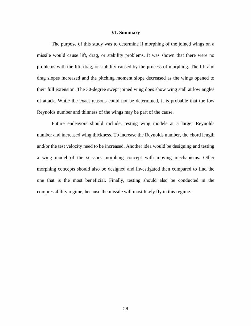
VI. Summary

The purpose of this study was to determine if morphing of the joined wings on a

missile would cause lift, drag, or stability problems. It was shown that there were no

problems with the lift, drag, or stability caused by the process of morphing. The lift and

drag slopes increased and the pitching moment slope decreased as the wings opened to

their full extension. The 30-degree swept joined wing does show wing stall at low angles

of attack. While the exact reasons could not be determined, it is probable that the low

Reynolds number and thinness of the wings may be part of the cause.

Future endeavors should include, testing wing models at a larger Reynolds

number and increased wing thickness. To increase the Reynolds number, the chord length

and/or the test velocity need to be increased. Another idea would be designing and testing

a wing model of the scissors morphing concept with moving mechanisms. Other

morphing concepts should also be designed and investigated then compared to find the

one that is the most beneficial. Finally, testing should also be conducted in the

compressibility regime, because the missile will most likely fly in this regime.

59

Appendix A

The following pages contain the lift and drag coefficient relations as well as pitch

and roll coefficient relations for all of the configurations tested.

60

-0.5

0

0.5

1

-10 0 10 20

Alpha

C_L


0

0.1

0.2

0.3

0.4

0.5

0.6

-0.5 0 0.5 1

C_L

C_D


Figure 53 Lift and drag relations of the bare missile.

61

-1

-0.5

0

0.5

1

-10 -5 0 5 10 15 20

Alpha

C_D


Figure 54 Drag relations of the bare missile.

62

-0.5

0

0.5

1

1.5

-10 0 10 20

Alpha

C_L


0

0.1

0.2

0.3

0.4

0.5

0.6

-0.5 0 0.5 1 1.5

C_L

C_D


Figure 55 Lift and drag Relations of 30o swept single wing located forward of CG, wings on bottom, aluminum.

63

-1

-0.5

0

0.5

1

-10 0 10 20

Alpha

C_D


-2.5

-2

-1.5

-1

-0.5

0

0.5

1

-10 -5 0 5 10 15 20

Alpha

C_m


Figure 56 Drag and pitch relations of the 30o swept single wing located forward of the CG, wings on bottom, aluminum.

64

-0.5

0

0.5

1

1.5

-10 0 10 20

Alpha

C_L


0

0.1

0.2

0.3

0.4

0.5

0.6

-0.5 0 0.5 1 1.5

C_L

C_D


Figure 57 Lift and drag relations of the 30o swept single wing located forward of the CG, wings on bottom, plastic.

65

-1

-0.5

0

0.5

1

-10 0 10 20

Alpha

C_D


-2.5

-2

-1.5

-1

-0.5

0

0.5

-10 0 10 20

Alpha

C_m


Figure 58 Drag and pitch relations of the 30o swept single wing located forward of the CG, wings on bottom, plastic.

66

-0.4

-0.2

0

0.2

0.4

0.6

0.8

1

1.2

1.4

-10 0 10 20

Alpha

C_L


0

0.1

0.2

0.3

0.4

0.5

0.6

-0.5 0 0.5 1 1.5

C_L

C_D


Figure 59 Lift and drag relations of 30o swept single wing located aft of CG, wings on top, aluminum.

67

-1

-0.5

0

0.5

1

-10 0 10 20

Alpha

C_D


-7

-6

-5

-4

-3

-2

-1

0

1

2

-10 -5 0 5 10 15 20

Alpha

C_m


Figure 60 Drag and pitch relations of the 30o swept single wing located aft of CG, wings on top, aluminum.

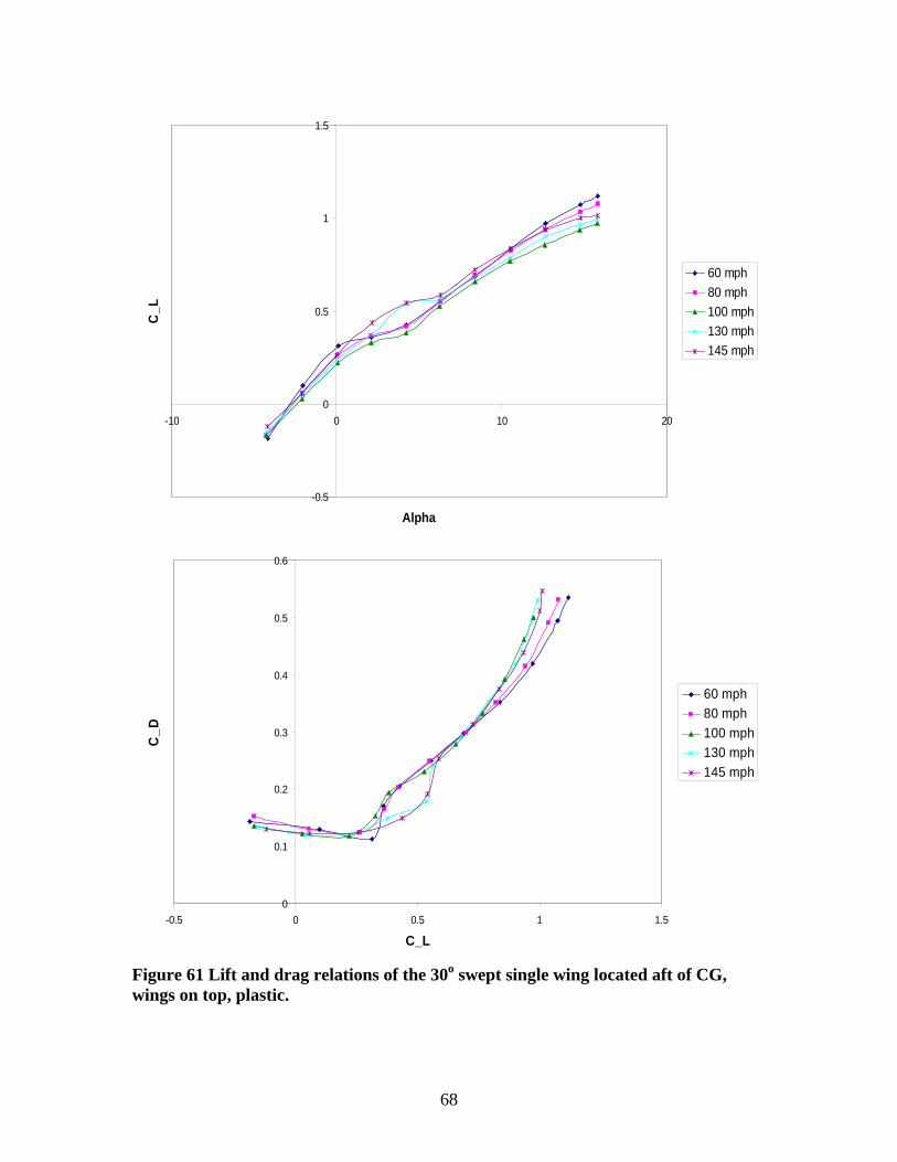
68

-0.5

0

0.5

1

1.5

-10 0 10 20

Alpha

C_L


0

0.1

0.2

0.3

0.4

0.5

0.6

-0.5 0 0.5 1 1.5

C_L

C_D


Figure 61 Lift and drag relations of the 30o swept single wing located aft of CG, wings on top, plastic.

69

-1

-0.5

0

0.5

1

-10 0 10 20

Alpha

C_D


-6

-5

-4

-3

-2

-1

0

1

2

-10 0 10 20

Alpha

C_m


Figure 62 Drag and pitch relations of the 30o swept single wing located aft of CG, wings on top, plastic.

70

-0.5

0

0.5

1

-10 0 10 20

Alpha

C_L


0

0.1

0.2

0.3

0.4

0.5

-0.5 0 0.5 1

C_L

C_D


Figure 63 Lift and drag relations of 30o swept joined wing, aluminum.

71

-1

-0.8

-0.6

-0.4

-0.2

0

0.2

0.4

0.6

0.8

1

-10 0 10 20

Alpha

C_D


-2.5

-2

-1.5

-1

-0.5

0

0.5

-10 0 10 20

Alpha

C_m


Figure 64 Drag and pitch relations of the 30o joined wing, aluminum.

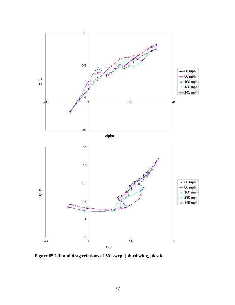
72

-0.5

0

0.5

1

-10 0 10 20

Alpha

C_L


0

0.1

0.2

0.3

0.4

0.5

-0.5 0 0.5 1

C_L

C_D


Figure 65 Lift and drag relations of 30o swept joined wing, plastic.

73

-1

-0.5

0

0.5

1

-10 0 10 20

Alpha

C_D


-2.5

-2

-1.5

-1

-0.5

0

0.5

-10 0 10 20

Alpha

C_m


Figure 66 Drag and pitch relations of the 30o joined wing, plastic.

74

-0.5

0

0.5

1

1.5

-10 0 10 20

Alpha

C_L


0

0.1

0.2

0.3

0.4

0.5

0.6

0.7

-0.5 0 0.5 1 1.5

C_L

C_D


Figure 67 Lift and drag relations of the 45o single wing swept forward, plastic.

75

-1

-0.5

0

0.5

1

-10 0 10 20

Alpha

C_D


-6

-5

-4

-3

-2

-1

0

1

2

-10 0 10 20

Alpha

C_m


Figure 68 Drag and pitch relations of the 45o single wing swept forward, plastic.

76

-0.5

0

0.5

1

1.5

-10 0 10 20

Alpha

C_L


0

0.05

0.1

0.15

0.2

0.25

0.3

0.35

0.4

0.45

-0.5 0 0.5 1 1.5

C_L

C_D


Figure 69 Lift and drag relations of the 45o joined wing, plastic.

77

-1

-0.5

0

0.5

1

-10 0 10 20

Alpha

C_D


-2.5

-2

-1.5

-1

-0.5

0

0.5

-10 0 10 20

Alpha

C_m



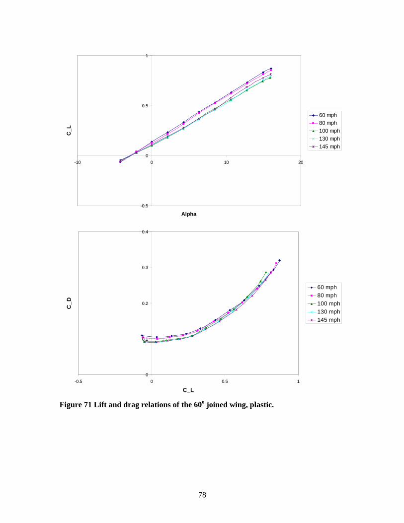
78

-0.5

0

0.5

1

-10 0 10 20

Alpha

C_L


0

0.1

0.2

0.3

0.4

-0.5 0 0.5 1

C_L

C_D



79

-1

-0.5

0

0.5

1

-10 0 10 20

Alpha

C_D


-2.5

-2

-1.5

-1

-0.5

0-10 -5 0 5 10 15 20

Alpha

C_m



80

-0.5

0

0.5

1

-10 0 10 20

Alpha

C_L


0

0.1

0.2

0.3

0.4

-0.5 0 0.5 1

C_L

C_D


Figure 73 Lift and drag relations of the 60o joined wing, plastic. Second Run.

81

-1

-0.5

0

0.5

1

-10 0 10 20

Alpha

C_D


-2.5

-2

-1.5

-1

-0.5

0-10 -5 0 5 10 15 20

Alpha

C_m


Figure 74 Drag and pitch relations of the 60o joined wing, plastic. Second Run.

82

-0.5

0

0.5

1

-10 0 10 20

Alpha

C_L


0

0.05

0.1

0.15

0.2

0.25

0.3

0.35

-0.5 0 0.5 1

C_L

C_D


Figure 75 Lift and drag relations of the 60o joined wing, not morphed, aluminum.

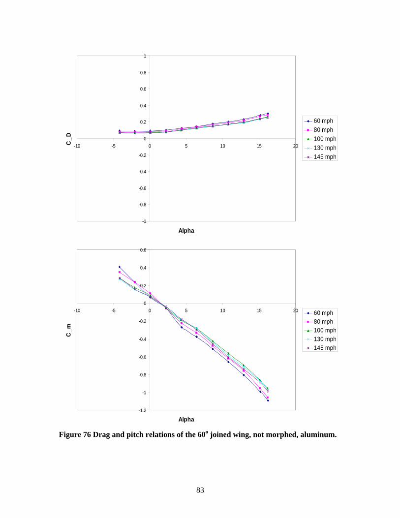
83

-1

-0.8

-0.6

-0.4

-0.2

0

0.2

0.4

0.6

0.8

1

-10 -5 0 5 10 15 20

Alpha

C_D


-1.2

-1

-0.8

-0.6

-0.4

-0.2

0

0.2

0.4

0.6

-10 -5 0 5 10 15 20

Alpha

C_m


Figure 76 Drag and pitch relations of the 60o joined wing, not morphed, aluminum.

84

-0.5

0

0.5

1

-10 0 10 20

Alpha

C_L


0

0.05

0.1

0.15

0.2

0.25

-0.5 0 0.5 1

C_L

C_D



85

-1

-0.5

0

0.5

1

-10 0 10 20

Alpha

C_D


-1.8

-1.6

-1.4

-1.2

-1

-0.8

-0.6

-0.4

-0.2

0

0.2

-10 0 10 20

Alpha

C_m



86

-0.5

0

0.5

1

-10 0 10 20

Alpha

C_L


0

0.05

0.1

0.15

0.2

0.25

-0.5 0 0.5 1

C_L

C_D



87

-1

-0.5

0

0.5

1

-10 0 10 20

Alpha

C_D


-1.8

-1.6

-1.4

-1.2

-1

-0.8

-0.6

-0.4

-0.2

0-10 0 10 20

Alpha

C_m



88

-0.5

0

0.5

1

-10 0 10 20

Alpha



Figure 81 Comparison of 60o joined wing between plastic morphed and the aluminum at 80 mph.

-0.5

0

0.5

1

-10 0 10 20

Alpha




89

-0.5

0

0.5

1

-10 0 10 20

Alpha




-0.5

0

0.5

1

-10 0 10 20

Alpha




90

-0.5

0

0.5

1

-10 0 10 20

Alpha

C_L Run 1

Run 2

Figure 85 Comparison between two Runs on the 60o plastic morphed wing testing for repetition at 60 mph.

-0.5

0

0.5

1

-10 0 10 20

Alpha

C_L Run 1

Run 2


91

-0.5

0

0.5

1

-10 0 10 20

Alpha

C_L Run 1

Run 2


-1

-0.5

0

0.5

1

-10 0 10 20

Alpha

C_L Run 1

Run 2


92

-3

-2

-1

0

1

2

3

4

-10 0 10 20

Alpha

L/D

30 deg JW30 deg Sing Top For30 deg Sing Bot Aft

Figure 89 Comparison of L/D vs Alpha for the 30o Joined wing and Single wings at 60 mph.

-3

-2

-1

0

1

2

3

4

-10 0 10 20

Alpha

L/D



93

-3

-2

-1

0

1

2

3

-10 0 10 20

Alpha

L/D



-3

-2

-1

0

1

2

3

4

-10 0 10 20

Alpha

L/D



94

-3

-2

-1

0

1

2

3

4

-10 0 10 20

Alpha

L/D



95

Appendix B

The following pages contain the MatLab code used to transfer measured forces

and moments on the balance to wind (Earth) centered frame reference by correcting for

tare effects, balance interactions, and wind tunnel irregularities, then outputting the lift,

drag, roll, pitch and yaw coefficients, as well as the angle of attack.

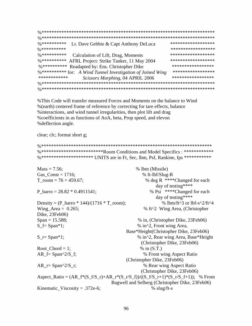
96

%********************************************************************** %********************************************************************** %********** Lt. Dave Gebbie & Capt Anthony DeLuca ****************** %********** ****************** %********** Calculation of Lift, Drag, Moments ****************** %********** AFRL Project: Strike Tanker, 11 May 2004 ****************** %********** Readapted by: Ens. Christopher Dike ***************** %********** for: A Wind Tunnel Investigation of Joined Wing ***************** ************ Scissors Morphing, 04 APRIL 2006 ***************** %********************************************************************** %********************************************************************** %This Code will transfer measured Forces and Moments on the balance to Wind %(earth) centered frame of reference by correcting for tare effects, balance %interactions, and wind tunnel irregularities, then plot lift and drag %coefficients in as functions of AoA, beta, Prop speed, and elevon %deflection angle. clear; clc; format short g; %********************************************************************* %*************************Room Conditions and Model Specifics : ************ %********************* UNITS are in Ft, Sec, lbm, Psf, Rankine, fps *********** Mass = 7.56; % lbm (Missile) Gas_Const = 1716; % ft-lbf/Slug-R T_room = 76 + 459.67; % deg R ****Changed for each day of testing**** P_barro = 28.82 * 0.4911541; % Psi ****Changed for each day of testing**** Density = (P_barro * 144)/(1716 * T_room); % lbm/ft^3 or lbf-s^2/ft^4 Wing_Area = 0.265; % ft^2 Wing Area, (Christopher Dike, 23Feb06) Span = 15.588; % in, (Christopher Dike, 23Feb06) S_f= Span*1; % in^2, Front wing Area, Base*Height(Christopher Dike, 23Feb06) S_r= Span*1; % in^2, Rear wing Area, Base*Height (Christopher Dike, 23Feb06) Root_Chord = 1; % in (S.T.) AR_f= Span^2/S_f; % Front wing Aspect Ratio (Christopher Dike, 23Feb06) AR_r= Span^2/S_r; % Rear wing Aspect Ratio (Christopher Dike, 23Feb06) Aspect_Ratio = (AR_f*(S_f/S_r)+AR_r*(S_r/S_f))/((S_f/S_r+1)*(S_r/S_f+1)); % From Bagwell and Selberg (Christopher Dike, 23Feb06) Kinematic_Viscosity = .372e-6; % slug/ft-s

97

Speed_of_Sound = sqrt(1.4 * T_room * Gas_Const); % fps %Distances between sensors (inches) to calculate moments D1 = (2.10 / 2); D2 = D1; D3 = (1.7 / 2); D4 = D3; %inches %Offset distances from the Mounting Block to the Model C.G. (inches) Y_cg = 0.0; % changed April 5 2006 >> Joined Wing Missile X_cg = 1.5625; % inches (from origin @ balance center w/ + right) Z_cg = 0.0; % inches (from origin @ balance center w/ + down) %********************************************************************** %*************************** Tunnel Correction Data ********************** %************************************************************************** K_1 = 1.08; % From fig. 10.2 assuming 4 digit airfoil K_3 = 0.89; % b/B, where B is 41 inches, the width of the tunnel delta = 0.38; Tau_1 = 0.83; X_Section = (32/12)*(41/12) ; % ft^2 Wing_Volume = Wing_Area * (.2/12) ; % ft^3 Body_Volume = (357.4./(12^3)); % ft^3 Epsilon_tunnel_correction=0.954742458; % Correction factor for velocity differences between Hot-wire and transducer 28 Feb 06 % For 100 > 0.955282636 , For 130 > 0.960305087 , For 145 > 0.954742458 %**** Solid body blockage corrections due to wing and fuselage *** Epsilon_sb_w = (K_1*Tau_1*Wing_Volume) / X_Section^(3/2); Epsilon_sb_b = (K_3*Tau_1*Body_Volume) / X_Section^(3/2); Epsilon_tot = Epsilon_sb_w + Epsilon_sb_b+(Epsilon_tunnel_correction-1); %********************************************************************** %*************************** Tunnel Correction Data ********************** %********************************************************************** %Balance Interactions with off axis elements for the 100 lb balance %Using average of the 8 lb calibration runs for N1 & N2 and the %6 lb calibration for S1, S2 & A then normalizing by the actual %sensor (N1, N2,...) in question. The sensor sequence in each row vector is:

98

% % [N1 N2 S1 S2 A L]N1_I = ([7.806 -.701 .447 .060 -.142 .043] + [7.803 -.702 .442 .057 -.140 .041])/2; % N11 = N1_I(1,1)/100; % % N2_I = ([.183 -7.486 -.05 -.052 .047 0] + [.182 -7.485 -.053 -.056 .044 0])/2; % N22 = N2_I(1,2)/-100; % % S1_I = ([.039 0 7.917 -.408 -.024 -.025] + [.036 0 7.915 -.410 -.026 -.022])/2; % S11 = S1_I(1,3)/50; % % S2_I = ([0 .013 -.124 8.16 -.067 -.017] + [0 .012 -.122 8.158 -.065 -.015])/2; % S22 = S2_I(1,4)/50; % % A_I = ([.012 .008 -.025 .041 6.981 0.09] + [.012 .007 -.025 .033 7.003 .081])/2; % A11 = A_I(1,5)/50; % % L_I = ([-.082 -.061 -.023 .096 .262 8.607] + [-.09 -.072 -.009 .104 .276 8.604])/2; % L11 = L_I(1,6)/40; %***** %*****Updated Calibration for the 8 component 25 lb, Ignoring A1 & L1 because of the similarity to A2 & L2 % and using an average of 10 lb calibration runs for N1, N2, S1, S2 & A2 and 7 lb for L2 then %dividing by its actual measurement to have a matrix of fractions with the diagonal of 1. N1_I = ([1 -.010272 .01244 -.000593 .13758 .014914]);%+ [7.803 -.702 .442 .057 -.140 .041])/2; HERE NUMBERS ARE lb/lb N11 = N1_I(1,1);%/100; N2_I = ([-.023 1 .00079 -.000296 .019354 .14516]); %+ [.182 -7.485 -.053 -.056 .044 0])/2; N22 = N2_I(1,2);%/-100; S1_I = ([.002864 .00593 1 .002963 .089481 .000099]); %+ [.036 0 7.915 -.410 -.026 -.022])/2; S11 = S1_I(1,3);%/50; S2_I = ([-.001576 .003939 -.026194 1 .028065 .007287]); %+ [0 .012 -.122 8.158 -.065 -.015])/2; S22 = S2_I(1,4);%/50; A_I = ([.209628 -.21866 .008038 -.007135 1 -.002077]); %+ [.012 .007 -.025 .033 7.003 .081])/2; A11 = A_I(1,5);%/50;

99

L_I = ([-.253931 -.239861 -.007284 .019533 .025824 1]); %+ [-.09 -.072 -.009 .104 .276 8.604])/2; L11 = L_I(1,6);%/40; N1_normalized = (N1_I) .* [N11 N22 S11 S22 A11 L11].^(-1); %/100) DROPPED FOR 25LB BALANCE N2_normalized = (N2_I) .* [N11 N22 S11 S22 A11 L11].^(-1); %/100) S1_normalized = (S1_I) .* [N11 N22 S11 S22 A11 L11].^(-1); %/50) S2_normalized = (S2_I) .* [N11 N22 S11 S22 A11 L11].^(-1); %/50) A_normalized = (A_I) .* [N11 N22 S11 S22 A11 L11].^(-1); %/50) L_normalized = (L_I) .* [N11 N22 S11 S22 A11 L11].^(-1); %/40) Interactions_Kij = [N1_normalized' N2_normalized' S1_normalized' S2_normalized' A_normalized' L_normalized']; %Load the static tare data for the alpha sweep w/o the wind , separate each %force from the file, and fit a 4th order poly as an x-y plot (AoA vs. %Force) for each of the 6 force sensors. %*************************Code inserted May 11, 2004********************** load Dike_Tare_30jwPl.txt; % Raw data file to be read in. FILE=Dike_Tare_30jwPl(:,:); j=1; k=1; L=length(FILE); for i=1:L %Run for all data points # of rows if i~=L %if current row is not last row, go to next NEXT=i+1; %set next equal to the value of the next row VALUE2=FILE(NEXT,1); %set value2 as next row column 1 else if i==L %unless the it is the last value VALUE2=50; %value2 set to 50 to end the sequence end end A(j,:)=FILE(i,:); %set row j of A equal to row i of FILE VALUE1=FILE(i,1); %set value1 equal to row i column 1 of FILE if VALUE1==VALUE2 %if value1 equals value2, go to next row j=j+1; else if VALUE1~=VALUE2 %if value1 and value2 are different check if length(A(:,1))<5 %if less than 20 values, ignored due to angle change j=1; clear A; else if length(A(:,1))>5 %if more than 20 values

100

C=length(A(:,1)); %find length of A for m=1:9 %Average all rows of the like values in A B(k,m)=mean(A(4:C,m)); %disregarding first 10 for vibrations end j=1; k=k+1; clear A end end end end end if B(k-1,1)<B((k-2),1) B=B(1:(k-2),:) end tare=[B] %******************************End of Inserted Code***************************** [row,col] = size(tare); for k = 1:row theta_tare(k,:,:) = tare(k,1).* (pi/180); N1_tare(k,:,:) = tare(k,4); N2_tare(k,:,:) = tare(k,5); S1_tare(k,:,:) = tare(k,7); S2_tare(k,:,:) = tare(k,8); A_tare(k,:,:) = tare(k,6); %changed 13Jan05 misnamed column L_tare(k,:,:) = tare(k,9); end N1_poly = polyfit(theta_tare,N1_tare,4); N2_poly = polyfit(theta_tare,N2_tare,4); S1_poly = polyfit(theta_tare,S1_tare,4); S2_poly = polyfit(theta_tare,S2_tare,4); A_poly = polyfit(theta_tare,A_tare,4) ; L_poly = polyfit(theta_tare,L_tare,4) ; clear ('B','C','D','L') %Load the specific test run files, subtract the effect of the static %weight with the tare polynominals above, and correct for cross diagonal

101

%sensor interactions. %*************************Code inserted May 11, 2004*************************** %modified January 11, 2005 load Dike_145_30jwPl.txt; % Raw data file to be read in: FILE=Dike_145_30jwPl(:,:); j=1; k=1; L=length(FILE); for i=1:L %Run for all data points # of rows if i~=L %if current row is not last row, go to next NEXT=i+1; %set next equal to the value of the next row VALUE2=FILE(NEXT,1); %set value2 as next row column 1 else if i==L %unless the it is the last value VALUE2=50; %value2 set to 50 to end the sequence end end A(j,:)=FILE(i,:); %set row j of A equal to row i of FILE VALUE1=FILE(i,1); %set value1 equal to row i column 1 of FILE if VALUE1==VALUE2 %if value1 equals value2, go to next row j=j+1; else if VALUE1~=VALUE2 %if value1 and value2 are different check if length(A(:,1))<5 %if less than 20 values, ignored due to angle change j=1; clear A; else if length(A(:,1))>5 %if more than 20 values C=length(A(:,1)); %find length of A for m=1:9 %Average all rows of the like values in A B(k,m)=mean(A(4:C,m)); %disregarding first 10 for vibrations end j=1; k=k+1; clear A end end end end end if B(k-1,1)<B((k-2),1) B=B(1:(k-2),:) end

102

sample_data=[B] %******************************End of Inserted Code***************************** [row2,col2] = size(sample_data); for i = 1:row2 %Angles of the model during test runs (Roll, Pitch {AoA}, Yaw {Beta}): phi = 0; theta(i,:) = sample_data(i,1) .* (pi/180); %radians si(i,:) = sample_data(i,2) .* (pi/180); %radians Wind_Speed(i,:) = sample_data(i,3) .* (5280/3600); %fps %pressure(i,:) = sample_data(i,(12:19)) - tare(i,12:19); %Flight Parameters (Re#, Ma#, Dynamic Pressure): q = (.5 * Density) .* Wind_Speed.^2; %lbf/ft^2 q_Corrected = q .* (1 + Epsilon_tot)^2; %lbf/ft^2 Wind_Speed_Corrected = Wind_Speed .* (1 + Epsilon_tot); %fps Mach_Number = Wind_Speed_Corrected ./ Speed_of_Sound; %NonDimensional Reynolds_Number = ((Density * Root_Chord) .* Wind_Speed_Corrected) ./ Kinematic_Viscosity; %NonDimensional Flight_Parameters = [Mach_Number Reynolds_Number q_Corrected]; %individual forces for each sensor: N1_test(i,:,:) = sample_data(i,4); N2_test(i,:,:) = sample_data(i,5); S1_test(i,:,:) = sample_data(i,7); S2_test(i,:,:) = sample_data(i,8); A_test(i,:,:) = sample_data(i,6); %changed 13Jan05 misnamed column L_test(i,:,:) = sample_data(i,9); %Evaluating the actual test theta angle (AoA) in the tare polynominal to %determine the tare values for the angles tested in each run. N1_eval = polyval(N1_poly,theta); N2_eval = polyval(N2_poly,theta); S1_eval = polyval(S1_poly,theta); S2_eval = polyval(S2_poly,theta); A_eval = polyval(A_poly,theta);

103

L_eval = polyval(L_poly,theta); %The Time-Averaged (raw) forces N1, N2, S1, S2, A, L measurd in the wind %tunnel (body axis) with the tare effect of the weight subtracted off. N1_resolved = N1_test - (N1_eval); N2_resolved = N2_test - (N2_eval); S1_resolved = S1_test - (S1_eval); S2_resolved = S2_test - (S2_eval); A_resolved = A_test - (A_eval); L_resolved = L_test - (L_eval); Forces_minus_tare = [N1_resolved N2_resolved S1_resolved S2_resolved A_resolved L_resolved]'; %Forces N1, N2, S1, S2, A, & L corrected for the balance interactions (body axis) Corrected_Data = (inv(Interactions_Kij) * Forces_minus_tare); %Calculation of the Axial, Side, & Normal Forces from the corrected balance %forces in the Body Axis reference frame Forces_b(:,i) = [Corrected_Data(5,i); Corrected_Data(3,i) + Corrected_Data(4,i); Corrected_Data(1,i) + Corrected_Data(2,i)]; %Calculation of the Drag, Side, & Lift Forces in the Wind Axis reference %frame Forces_w = [Forces_b(1,:).*cos(theta').*cos(si')+Forces_b(2,:).*sin(si')+Forces_b(3,:).*sin(theta').*cos(si'); -Forces_b(1,:).*sin(si').*cos(theta')+Forces_b(2,:).*cos(si')-Forces_b(3,:).*sin(theta').*sin(si'); -Forces_b(1,:).*sin(theta')+Forces_b(3,:).*cos(theta')]; %First entry is the moments calculated by the balance or direct calculation %in the Body Reference Frame. Balance measures Roll (l), Yaw is about the %z-axis (n), and Pitch is about the y-axis (m). Distances from strain %gages to C.G. are in INCHES. Moments are in-lbf m = Corrected_Data(1,i) * D1 - Corrected_Data(2,i) * D2; n = Corrected_Data(3,i) * D3 - Corrected_Data(4,i) * D4; Moments_b(:,i) = [Corrected_Data(6,i); m; n]; %Second entry is the conversion from the "Balance Centeric" moments to the %Wind Reference monments with respect to the Balance Center (bc)

104

Moments_w_bc = [Moments_b(1,:).*cos(theta').*cos(si')-Moments_b(2,:).*sin(si')+Moments_b(3,:).*sin(theta').*cos(si'); Moments_b(1,:).*sin(si').*cos(theta')+Moments_b(2,:).*cos(si')+Moments_b(3,:).*sin(theta').*sin(si'); -Moments_b(1,:).*sin(theta')+Moments_b(3,:).*cos(theta')]; %Finally, the balance centered moments are converted to moments about the %Model's Center of Mass (cm) or Center of Gravity (CG) cgdist=sqrt((X_cg)^2+(Z_cg)^2); %Obtaining the direct distance between the %center of the balance and the center of mass w=atan(-Z_cg/X_cg); %Obtaining the angle between cgdist and the x axes at zero angle of attack X_cm(i,:)= cos(theta(i,:)+w)*cos(si(i,:))*(cgdist); Y_cm(i,:) = Y_cg + X_cm(i,:)*tan(si(i,:)); % appropriate for very small y_cmb and reasonable si Z_cm(i,:)= -sin(theta(i,:)+w)*(cgdist); Moments_w_cg_u = [Moments_w_bc(1,:) + Z_cm(i,:)*Forces_w(2,:) + Forces_w(3,:)* Y_cm(i,:); Moments_w_bc(2,:) - X_cm(i,:)*Forces_w(3,:) + Forces_w(1,:)* Z_cm(i,:); Moments_w_bc(3,:) - Y_cm(i,:)*Forces_w(1,:) - Forces_w(2,:)* X_cm(i,:)]; %Calculation of the actual Lift and Drag non-dimensional Coefficients, uncorrected for tunnel effects, (Cl and Cd) C_L_u = Forces_w(3,:) ./ (q_Corrected' .* Wing_Area); %Keuthe & Chow pg 178 C_D_u = Forces_w(1,:) ./ (q_Corrected' .* Wing_Area); Coefficients = [C_L_u; C_D_u]'; % Ave_Cl = mean(Coefficients(:,1)); % Ave_Cd = mean(Coefficients(:,2)); end %********************************************************************** %*************************** Tunnel Correction Data ********************** %************************************************************************** %****************** Drag Coefficient Correction *************** C_D_o = min(Coefficients(:,2)); C_L_u_sqrd = Coefficients(:,1).^2;

105

Delta_C_D_w = ((delta * Wing_Area) / X_Section) .* C_L_u_sqrd; C_D_Corrected = C_D_u' + Delta_C_D_w; %************* Angle of Attack due to upwash Correction ********* alpha = sample_data(:,1); Delta_alpha_w = ((delta * Wing_Area) / X_Section) .* (57.3 * C_L_u); alpha_Corrected = alpha + Delta_alpha_w'; %************* Pitching Moment Correction *********************** tau2 = .6; % Blockage of horizontal tail from Fig 10.40 of Wind Tunnel book l_t = 12.26/12; % ft = length from tail MAC to aircraft CG Span_t = 5/ 12 ; % ft = Projected horizontal span of V-tail Tail_Area = 4.375/ 144; % ft^2 = Projected horizontal tail area c_bar = 1 / 12; % 1.6875 13 Sept 04 Changed May 11, 2004 ft = Mean Chord of wing *** %Changed again April 4, 2006 V_bar = (Tail_Area * l_t) / (Wing_Area * c_bar); % Horizontal tail volume ratio eta_t = 1.0; epsilon_o = 0; i_t = 0; % radians i_w = 0; Aspect_Ratio_t = Span_t^2 / Tail_Area; D_epslion_D_alpha = ((2 .* C_L_u) ./ (pi* Aspect_Ratio))'; epsilon = epsilon_o + (D_epslion_D_alpha .* alpha_Corrected ); alpha_t = alpha_Corrected - i_w - epsilon + i_t; C_L_alpha_t = ((0.1* Aspect_Ratio_t) / (Aspect_Ratio_t +2)) * 0.8; D_Cm_cg_t_D_alpha_t = -C_L_alpha_t* V_bar * eta_t; Delta_C_m_cg_t = ((D_Cm_cg_t_D_alpha_t) * (delta*tau2) * (Wing_Area / X_Section) .* (C_L_u * 57.3))'; Cl_w_cg = Moments_w_cg_u(1,:) ./ (q_Corrected' .* (Wing_Area * Span*12)); Cm_w_cg_u = Moments_w_cg_u(2,:) ./ (q_Corrected' .* (Wing_Area * c_bar*12)); Cn_w_cg = Moments_w_cg_u(3,:) ./ (q_Corrected' .* (Wing_Area * Span*12)); Cm_w_cg_corrected = Cm_w_cg_u - Delta_C_m_cg_t'; Corrected_Moment_Coefficients = [Cl_w_cg' Cm_w_cg_corrected' Cn_w_cg']; %********************************************************************** %*************************** Tunnel Correction Data ********************** %************************************************************************** alpha = sample_data(:,1);

106

fprintf(' Mach Number Reynolds Number Dynamic Pressure(Psf)\r') Flight_Parameters fprintf(' \r'); fprintf(' Loads are in lbf and arranged [D S L] across the top and increments of alpha down the side \r') Forces_w' fprintf(' \r') fprintf(' Moments are in in-lbf and arranged [L M N] down the side and increments of alpha along the top \r') Moments_w_cg_u fprintf(' \r') fprintf(' Cl_u Cd_u \r'); Coefficients fprintf(' \r') fprintf(' Del_CD_w CD_u CD_Corrected \r'); Compare_CD = [Delta_C_D_w C_D_u' C_D_Corrected] fprintf(' \r') fprintf(' Del_alpha_w alpha_g alpha_Corrected \r'); Compare_alpha = [Delta_alpha_w' alpha alpha_Corrected ] fprintf(' \r') fprintf(' Cl_cg_wind Cm_cg_corrected_w Cn_cg_wind \r'); Corrected_Moment_Coefficients fprintf(' \r') fprintf(' M# Re# q_c Uoo alpha_c C_L C_D_c Cl_cg_w Cm_cg_c_w Cn_cg_w \r'); YY=[Flight_Parameters (Wind_Speed_Corrected .* (3600/5280)) alpha_Corrected C_L_u' C_D_Corrected Corrected_Moment_Coefficients]%pressure] %XX=['M#' 'Re#' 'q_c' 'Uoo' 'alpha_c' 'C_L' 'C_D_c' 'Cl_cg_w' 'Cm_cg_c_w' 'Cn_cg_w \r']; %******UNUSED CODE %ZZ=[XX; YY]; wk1write('output.xls',YY,2,1) % Max_Cl = max(Coefficients(:,1)); % figure(6); % % subplot ('position',[.15 .6 .3 .3]); % plot(alpha_Corrected,Coefficients(:,1),'b-'); grid on % legend('30 mph'); % title('\it Flex Wing MAV: C_L_u vs \alpha '); xlabel('Angle of Attack (\alpha)'); ylabel('Lift Coefficient (C_L_u'); % % subplot ('position',[.65 .6 .3 .3]); % plot(alpha_Corrected,Coefficients(:,2),'b',alpha_Corrected,C_D_Corrected,'r'); grid on

107

% legend('C_D_u', 'C_D_c'); % title('\it Flex Wing MAV: C_D vs \alpha'); xlabel('Angle of Attack (\alpha)'); ylabel('Drag Coefficient (C_D)'); % % subplot('position',[.15 .1 .3 .3]); % plot(Coefficients(:,2),Coefficients(:,1),'b',C_D_Corrected,Coefficients(:,1),'r'); grid on % legend('C_D_u', 'C_D_c'); % title('\it Flex Wing MAV: C_L_u vs C_D'); xlabel('Drag Coefficient (C_D)'); ylabel('Lift Coefficient (C_L_u )'); % % subplot ('position',[.65 .1 .3 .3]) % plot(Coefficients(:,2),Coefficients(:,1).^2,'b',C_D_Corrected,Coefficients(:,1).^2,'r'); grid on % legend('C_D_u', 'C_D_c'); % title('\it Flex Wing MAV: C_L_u ^2 vs C_D'); xlabel('Drag Coefficient (C_D)'); ylabel('Lift Coefficient (C_L_u ^2)'); %************************************************************************** %************************************************************************** % % % % figure(7); % plot(alpha,Coefficients(:,1),'b.-.',... % alpha,Coefficients2(:,1),'r.:',... % alpha,Coefficients3(:,1),'k.-',... % alpha,Coefficients4(:,1),'m.--'); % legend('30 mph (Re_c\approx 130K)','60 mph (Re_c\approx 260K)','90 mph (Re_c\approx 390K)','\beta \approx 10\circ'); grid on; % title('\it C_L vs \alpha','FontWeight','bold','FontSize',11); xlabel('Angle of Attack (\alpha)'); ylabel('Lift Coefficient (C_L)'); % % figure(8); % plot(alpha,Coefficients(:,2),'b.-.',... % alpha,Coefficients2(:,2),'r.:',... % alpha,Coefficients3(:,2),'k.-',... % alpha,Coefficients4(:,2),'m.--'); % legend('30 mph (Re_c\approx 130K)','60 mph (Re_c\approx 260K)','90 mph (Re_c\approx 390K)','\beta \approx 10\circ'); grid on; % title('\it C_D vs \alpha','FontWeight','bold','FontSize',11); xlabel('Angle of Attack (\alpha)'); ylabel('Drag Coefficient (C_D)'); %

108

% figure(9); % plot(Coefficients(:,2),Coefficients(:,1),'b.-.',... % Coefficients2(:,2),Coefficients2(:,1),'r.:',... % Coefficients3(:,2),Coefficients3(:,1),'k.-',... % Coefficients4(:,2),Coefficients4(:,1),'m.--'); % legend('30 mph (Re_c\approx 130K)','60 mph (Re_c\approx 260K)','90 mph (Re_c\approx 390K)','\beta \approx 10\circ'); grid on; % title('\it C_L vs C_D','FontWeight','bold','FontSize',11); xlabel('Drag Coefficient (C_D)'); ylabel('Lift Coefficient (C_L)'); % % figure(10); % plot(Coefficients(:,2),Coefficients(:,1).^2,'b.-.',... % Coefficients2(:,2),Coefficients2(:,1).^2,'r.:',... % Coefficients3(:,2),Coefficients3(:,1).^2,'k.-',... % Coefficients4(:,2),Coefficients4(:,1).^2,'m.--'); % legend('30 mph (Re_c\approx 130K)','60 mph (Re_c\approx 260K)','90 mph (Re_c\approx 390K)','\beta \approx 10\circ'); grid on; % title('\it C_L ^2 vs C_D','FontWeight','bold','FontSize',11); xlabel('Drag Coefficient (C_D)'); ylabel('Lift Coefficient (C_L)^2'); % % figure(11); % plot(REYNOLDS_NUM, MAX_CL,'.-'); grid on % title('\it C_L _(_M_a_x_) vs Reynolds Number (Re_c )', 'FontWeight','bold', 'FontSize', 10); % xlabel('Chord Reynolds Number'); ylabel('Maximum Lift Coefficient (C_L _M_a_x_)'); % % figure(12); % plot(REYNOLDS_NUM, MIN_CD,'.-'); grid on; % title('\it C_D_o _(_M_i_n_) vs Reynolds Number (Re_c )', 'FontWeight','bold', 'FontSize', 10); % xlabel('Chord Reynolds Number'); ylabel('Minimum Drag Coefficient (C_D _M_i_n)'); % % figure(13) % plot(REYNOLDS_NUM, CD_Lam,'.-',REYNOLDS_NUM, CD_Turb,'.--'); grid on; % title('\it C_D_(_S_k_i_n_ _F_r_i_c_t_i_o_n_) vs Reynolds Number (Re_c )', 'FontWeight','bold', 'FontSize', 10); % xlabel('Chord Reynolds Number'); ylabel('Drag Coefficient (C_D )'); % legend('Laminar', 'Turbulent'); % % %figure(14); % %plot(alpha,Actual_Loads(2,:)); % %title('\it Side Force vs \alpha (60 mph & \beta = 10^o )', 'FontWeight','bold', 'FontSize', 10'); % %xlabel('Angle of Attack (\alpha)'); ylabel('Side Force (Lb_f )');

109

Bibliography

1. Aeroelastic Analysis and Optimization on Joined-Wing Configurations. Dir. Dong-Hwan

Lee and P. C. Chen. Slide Program. Zona Technology. 2. Bagwill, Tracy L., and Bruce P. Selberg. "Aerodynamic Investigation of Joined Wing

Configurations for Transport Aircraft." AIAA 96-2373-CP: 30-41. 3. Bagwill, Tracy L., and Bruce P. Selberg. Aerodynamic Investigation of Twist and Cant

Angles for Joined Wing Transport Aircraft. 35th Aerospace Sciences Meeting & Exhibit, 6-10 Jan. 1997. AIAA 97-0037.

4. Bertin, John J. Aerodynamics for Engineers. 4th ed. Upper Saddle, New Jersey: Prentice Hall, 2002. 413-417.

5. Cole, Stanley R. "Divergence Study of a High-Aspect Ratio, Forward Swept Wing." AIAA 86-0009.

6. Corneille, Jennifer. Wind Tunnel Investigation of Joined Wing Configurations. Dept. of the Air Force Air University. Wright-Patterson AFB, Ohio: Air Force Institute of Technology, 1999.

7. Gall, Peter D. "Aerodynamic Characteristics of Biplanes with Winglets." Journal of Aircraft 2nd ser. 24 (1987): 518-522.

8. Guiler, Richard, and Dr. Wade Huebsch. Wind Tunnel Analysis of a Morphing Swept Wing Tailless Aircraft. Applied Aerodynamics Conference, 6-9 June 2005. AIAA 2005-4981.

9. Hixenbaugh, John W. Digital image. [Hotwire Test Pattern]. 2006. Air Force Institute of Technology. 15 Apr. 2006.

10. Hoang, Ty, and Danielle S. Soban. Technology Advancements as Applied to Six Subsonic Transports. Aircraft Design, Systems and Operations Meeting. AIAA 93-3950.

11. Jones, Brent L. Experimental Investigation into the Aerodynamic Ground Effect of a Tailless Chevron-Shaped UCAV. Dept. of the Air Force Air University. Wright-Patterson AFB, Ohio: Air Force Institute of Technology, 2005.

12. Katz, Joseph, Shaun Byrne, and Robert Hahl. "Stall Resistance Features of Lifting-Body Airplane Configurations." Journal of Aircraft 2nd ser. 36 (1999): 471-474.

13. Kress, Robert W. "Variable Sweep Wing Design." AIAA 83-1051: 43-61.

110

14. Kroo, Ilan, John Gallman, and Stephen Smith. "Aerodynamic and Structural Studies of Joined-Wing Aircraft." Journal of Aircraft 28 (1991): 74-81.

15. Kulhman, J M., and T J. Ku. "Numerical Optimization Techniques for Bound Circulation Distribution for Minimum Induced Drag of Non-Planar Wings: Computer Program Documentation." NASA CR-3458 (1982).

16. Mostaccio, Jason. Digital image. [Placement of Hotwire Anemometer]. 2006. Air Force Institute of Technology. 3 Apr. 2006.

17. Nelson, Robert C. Flight Stability and Automatic Control. 2nd ed. WCB/McGraw-Hill, 1998.

18. Perkins, J N., F M. Cheatwood, R J. Vess, and R A. Wahls. The Design and Testing of Several Joined Wing RPV's. AIAA 23rd Aerospace Sciences Meeting, 14-17 Jan. 1985. AIAA 85-0275.

19. Raymer, Daniel P. Aircraft Design: a Conceptual Approach. 3rd ed. AIAA, 1999.

20. Ron Dupas Collection. 29 Aug. 2002. 4 Apr. 2006 <http://1000aircraftphotos.com/Biplanes/1737L.jpg>.

21. Selberg, B P., and D L. Cronin. Aerodynamic - Structural Optimization of Positive/Negative Stagger Joined Wing Configurations. Aircraft Systems, Design, & Technology Meeting. AIAA 86-2626.

22. Wolkovitch, Julian. Application of the Joined Wing to Cruise Missiles: Final Report for Phase 1. Contract N00014-79-C-0953, Rancho Palos Verdes, CA: Aeronautical Consultant Associates, November 1980 (AD-A096450).

23. Wolkovitch, Julian. The Joined Wing: an Overview. AIAA 23rd Aerospace Sciences Meeting, 14-17 Jan. 1985. AIAA 85-0274.

REPORT DOCUMENTATION PAGE Form Approved OMB No. 074-0188

The public reporting burden for this collection of information is estimated to average 1 hour per response, including the time for reviewing instructions, searching existing data sources, gathering and maintaining the data needed, and completing and reviewing the collection of information. Send comments regarding this burden estimate or any other aspect of the collection of information, including suggestions for reducing this burden to Department of Defense, Washington Headquarters Services, Directorate for Information Operations and Reports (0704-0188), 1215 Jefferson Davis Highway, Suite 1204, Arlington, VA 22202-4302. Respondents should be aware that notwithstanding any other provision of law, no person shall be subject to an penalty for failing to comply with a collection of information if it does not display a currently valid OMB control number. PLEASE DO NOT RETURN YOUR FORM TO THE ABOVE ADDRESS. 1. REPORT DATE (DD-MM-YYYY) 13-Jun-2006

2. REPORT TYPE Master’s Thesis

3. DATES COVERED (From – To) Jun 2005 – Jun 2006

5a. CONTRACT NUMBER

5b. GRANT NUMBER

4. TITLE AND SUBTITLE A Wind Tunnel Investigation of Joined Wing Scissors Morphing 5c. PROGRAM ELEMENT NUMBER

5d. PROJECT NUMBER 5e. TASK NUMBER

6. AUTHOR(S) Dike, Christopher C., Ensign, USN 5f. WORK UNIT NUMBER

7. PERFORMING ORGANIZATION NAMES(S) AND ADDRESS(S) Air Force Institute of Technology Graduate School of Engineering and Management (AFIT/EN) 2950 Hobson Way WPAFB OH 45433-7765

8. PERFORMING ORGANIZATION REPORT NUMBER AFIT/GAE/ENY/06-J02

10. SPONSOR/MONITOR’S ACRONYM(S)

9. SPONSORING/MONITORING AGENCY NAME(S) AND ADDRESS(ES) N/A

11. SPONSOR/MONITOR’S REPORT NUMBER(S)

12. DISTRIBUTION/AVAILABILITY STATEMENT APPROVED FOR PUBLIC RELEASE; DISTRIBUTION UNLIMITED.

13. SUPPLEMENTARY NOTES 14. ABSTRACT The Air Force Research Laboratory’s Munitions Directorate has been looking to extend the range of its small smart bomb. Corneille [6] has conducted tests to determine the aerodynamic characteristics of joined wings on a missile and determine if joined wings are more beneficial than a single wing configuration. The concept of retrofitting wings on the bomb introduced an interesting problem: storage before deployment. This study conducted steady-state low speed wind tunnel testing of a joined wing configuration that morphed from a compact configuration for storage to a full extension. These steady-state tests examine differing sweep angles of the same joined wing configuration. The lift and drag as well as pitching moments and rolling moments were determined and analyzed for the effects of morphing.

15. SUBJECT TERMS Morphing; Variable Sweep; Extended Range Missile; Wind Tunnel Testing; Joined Wing;

16. SECURITY CLASSIFICATION OF:

19a. NAME OF RESPONSIBLE PERSON Milton Franke, Dr. (ENY)

REPORT U

ABSTRACT U

c. THIS PAGE U

17. LIMITATION OF ABSTRACT UU

18. NUMBER OF PAGES 128 19b. TELEPHONE NUMBER (Include area code)

(937) 786-3636, ext 4720; e-mail: [email protected]

Standard Form 298 (Rev: 8-98) Prescribed by ANSI Std. Z39-18

air force institute of technology - dtic.mil · iv afit/gae/eny/06-j02 abstract the air force...

Documents