air force institute of technologyvibration interaction in a multiple flywheel system thesis jordan...
TRANSCRIPT
Vibration Interaction in aMultiple Flywheel System
THESIS
Jordan Firth, Captain, USAF
AFIT/GA/ENY/11-M03
DEPARTMENT OF THE AIR FORCEAIR UNIVERSITY
AIR FORCE INSTITUTE OF TECHNOLOGY
Wright-Patterson Air Force Base, Ohio
APPROVED FOR PUBLIC RELEASE; DISTRIBUTION UNLIMITED


The views expressed in this thesis are those of the author and do not reflect the officialpolicy or position of the United States Air Force, the Department of Defense, or theUnited States Government. This material is declared a work of the U.S. Governmentand is not subject to copyright protection in the United States.

AFIT/GA/ENY/11-M03
Vibration Interaction in a
Multiple Flywheel System
THESIS
Presented to the Faculty
Department of Aeronautics and Astronautics
Graduate School of Engineering and Management
Air Force Institute of Technology
Air University
Air Education and Training Command
In Partial Fulfillment of the Requirements for the
Degree of Master of Science in Astronautical Engineering
Jordan Firth, B.S. Engineering Mechanics
Captain, USAF
March 2011
APPROVED FOR PUBLIC RELEASE; DISTRIBUTION UNLIMITED

AFIT/GA/ENY/11-M03
Abstract
This study uses a linear model of an Integrated Power and Attitude Control
System (IPACS) to investigate the vibration interaction between multiple flywheels.
An easily extendable Matlab® script is created for the analysis of flywheel vibra-
tions. This script is used to build a vibration model consisting of two active magnetic
bearing flywheels mounted on a support structure. The flywheels are rotated at vary-
ing speeds, with an imbalance-induced centripetal force in one or both wheels causing
vibrations in both wheels. Flywheel and system responses are examined for low fre-
quency vibrations which would cause undesirable excitation to a satellite using IPACS,
with a specific focus on the beat phenomenon and extra-synchronous vibration. Extra-
synchronous resonant vibration between multiple rotors is shown to exist in an ideal
undamped configuration but even a very small realistic amount of damping is enough
to mitigate the effect enough that it is of less concern than individual rotor vibration
inputs. Extra-synchronous resonant vibration is thus shown to have a minimal effect
on satellite IPACS operation.
iv

I Corinthians 10:31
v

Acknowledgements
Writing this thesis was more difficult than I had anticipated, and I could not
have done it without significant help along the way. Dr. Black, thanks for your con-
tinual encouragement from beginning to end. Dr. Cobb and Dr. Swenson, thank you
for saving future readers from a miry swamp of confusion. To my fellow late night
Astro lab inhabitants, thanks for the energy.
And of course, many many thanks to my loving and incredible wife, who fed
and took care of me during a grueling 5 months.
Jordan Firth
vi

Table of ContentsPage
Abstract . . . . . . . . . . . . . . . . . . . . . . . . . . . . . . . . . . . . . . . . . . . . . . . . . . . . . . . . . . . . . . . . . . . . . . . . . . . . . . . . iv
Acknowledgements . . . . . . . . . . . . . . . . . . . . . . . . . . . . . . . . . . . . . . . . . . . . . . . . . . . . . . . . . . . . . . . . . . . . vi
List of Figures . . . . . . . . . . . . . . . . . . . . . . . . . . . . . . . . . . . . . . . . . . . . . . . . . . . . . . . . . . . . . . . . . . . . . . . . . ix
List of Tables . . . . . . . . . . . . . . . . . . . . . . . . . . . . . . . . . . . . . . . . . . . . . . . . . . . . . . . . . . . . . . . . . . . . . . . . . . xi
List of Acronyms . . . . . . . . . . . . . . . . . . . . . . . . . . . . . . . . . . . . . . . . . . . . . . . . . . . . . . . . . . . . . . . . . . . . . . xii
Nomenclature . . . . . . . . . . . . . . . . . . . . . . . . . . . . . . . . . . . . . . . . . . . . . . . . . . . . . . . . . . . . . . . . . . . . . . . . . . xiii
I. Introduction . . . . . . . . . . . . . . . . . . . . . . . . . . . . . . . . . . . . . . . . . . . . . . . . . . . . . . . . . . . . . . . . . . . . . . 11.1 Definitions . . . . . . . . . . . . . . . . . . . . . . . . . . . . . . . . . . . . . . . . . . . . . . . . . . . . . . . . . . . . . . . . . . . 11.2 Overview . . . . . . . . . . . . . . . . . . . . . . . . . . . . . . . . . . . . . . . . . . . . . . . . . . . . . . . . . . . . . . . . . . . . . 21.3 Objectives. . . . . . . . . . . . . . . . . . . . . . . . . . . . . . . . . . . . . . . . . . . . . . . . . . . . . . . . . . . . . . . . . . . . 5
1.4 Organization . . . . . . . . . . . . . . . . . . . . . . . . . . . . . . . . . . . . . . . . . . . . . . . . . . . . . . . . . . . . . . . . . 6
II. Background . . . . . . . . . . . . . . . . . . . . . . . . . . . . . . . . . . . . . . . . . . . . . . . . . . . . . . . . . . . . . . . . . . . . . . . 7
2.1 Literature Review . . . . . . . . . . . . . . . . . . . . . . . . . . . . . . . . . . . . . . . . . . . . . . . . . . . . . . . . . . . 72.2 Coordinates and Nomenclature . . . . . . . . . . . . . . . . . . . . . . . . . . . . . . . . . . . . . . . . . . . . 132.3 Fundamental Equations . . . . . . . . . . . . . . . . . . . . . . . . . . . . . . . . . . . . . . . . . . . . . . . . . . . . . 14
2.3.1 Equation of Motion for a Gyroscopic Body. . . . . . . . . . . . . . . . . . . . . . . . 14
2.3.2 State-Space Equation of Motion . . . . . . . . . . . . . . . . . . . . . . . . . . . . . . . . . . . . 15
2.3.3 Rotated Equation of Motion . . . . . . . . . . . . . . . . . . . . . . . . . . . . . . . . . . . . . . . . 16
2.3.4 Centripetal Force . . . . . . . . . . . . . . . . . . . . . . . . . . . . . . . . . . . . . . . . . . . . . . . . . . . . 17
2.3.5 Natural Frequencies of a Rotor/Bearing System . . . . . . . . . . . . . . . . . . 17
2.3.6 Beat Frequency . . . . . . . . . . . . . . . . . . . . . . . . . . . . . . . . . . . . . . . . . . . . . . . . . . . . . . 22
2.4 Model . . . . . . . . . . . . . . . . . . . . . . . . . . . . . . . . . . . . . . . . . . . . . . . . . . . . . . . . . . . . . . . . . . . . . . . . 252.5 Scope . . . . . . . . . . . . . . . . . . . . . . . . . . . . . . . . . . . . . . . . . . . . . . . . . . . . . . . . . . . . . . . . . . . . . . . . . 25
III. Methodology . . . . . . . . . . . . . . . . . . . . . . . . . . . . . . . . . . . . . . . . . . . . . . . . . . . . . . . . . . . . . . . . . . . . . . 27
3.1 Overview . . . . . . . . . . . . . . . . . . . . . . . . . . . . . . . . . . . . . . . . . . . . . . . . . . . . . . . . . . . . . . . . . . . . . 273.2 Model Description . . . . . . . . . . . . . . . . . . . . . . . . . . . . . . . . . . . . . . . . . . . . . . . . . . . . . . . . . . . 27
3.2.1 Model Construction . . . . . . . . . . . . . . . . . . . . . . . . . . . . . . . . . . . . . . . . . . . . . . . . . 273.2.2 Model Inputs. . . . . . . . . . . . . . . . . . . . . . . . . . . . . . . . . . . . . . . . . . . . . . . . . . . . . . . . . 29
3.2.3 Model Parameters . . . . . . . . . . . . . . . . . . . . . . . . . . . . . . . . . . . . . . . . . . . . . . . . . . . 313.3 System Equation of Motion . . . . . . . . . . . . . . . . . . . . . . . . . . . . . . . . . . . . . . . . . . . . . . . . 32
3.3.1 System Equation of Motion Components . . . . . . . . . . . . . . . . . . . . . . . . . . 32
vii

Page
3.3.2 System Equation of Motion Assembly . . . . . . . . . . . . . . . . . . . . . . . . . . . . . 37
3.4 Integration . . . . . . . . . . . . . . . . . . . . . . . . . . . . . . . . . . . . . . . . . . . . . . . . . . . . . . . . . . . . . . . . . . . 40
3.5 Additional Components . . . . . . . . . . . . . . . . . . . . . . . . . . . . . . . . . . . . . . . . . . . . . . . . . . . . . 41
3.5.1 Appendage . . . . . . . . . . . . . . . . . . . . . . . . . . . . . . . . . . . . . . . . . . . . . . . . . . . . . . . . . . . 41
3.5.2 Satellite/support spring . . . . . . . . . . . . . . . . . . . . . . . . . . . . . . . . . . . . . . . . . . . . . 42
3.6 Validation . . . . . . . . . . . . . . . . . . . . . . . . . . . . . . . . . . . . . . . . . . . . . . . . . . . . . . . . . . . . . . . . . . . . 423.6.1 Validation Inputs . . . . . . . . . . . . . . . . . . . . . . . . . . . . . . . . . . . . . . . . . . . . . . . . . . . . 42
3.7 Summary. . . . . . . . . . . . . . . . . . . . . . . . . . . . . . . . . . . . . . . . . . . . . . . . . . . . . . . . . . . . . . . . . . . . . 48
IV. Results and Analysis . . . . . . . . . . . . . . . . . . . . . . . . . . . . . . . . . . . . . . . . . . . . . . . . . . . . . . . . . . . . . 50
4.1 Full Envelope Sweep . . . . . . . . . . . . . . . . . . . . . . . . . . . . . . . . . . . . . . . . . . . . . . . . . . . . . . . . 50
4.2 Beat Frequency Analysis. . . . . . . . . . . . . . . . . . . . . . . . . . . . . . . . . . . . . . . . . . . . . . . . . . . . 54
4.3 Extra-Synchronous Whirl Excitation . . . . . . . . . . . . . . . . . . . . . . . . . . . . . . . . . . . . . . 58
4.3.1 Sub-Synchronous Whirl Excitation . . . . . . . . . . . . . . . . . . . . . . . . . . . . . . . . . 58
4.3.2 Super-synchronous Whirl Excitation . . . . . . . . . . . . . . . . . . . . . . . . . . . . . . . 64
4.4 Summary. . . . . . . . . . . . . . . . . . . . . . . . . . . . . . . . . . . . . . . . . . . . . . . . . . . . . . . . . . . . . . . . . . . . . 68
V. Conclusion . . . . . . . . . . . . . . . . . . . . . . . . . . . . . . . . . . . . . . . . . . . . . . . . . . . . . . . . . . . . . . . . . . . . . . . . 705.1 Summary. . . . . . . . . . . . . . . . . . . . . . . . . . . . . . . . . . . . . . . . . . . . . . . . . . . . . . . . . . . . . . . . . . . . . 70
5.2 Findings . . . . . . . . . . . . . . . . . . . . . . . . . . . . . . . . . . . . . . . . . . . . . . . . . . . . . . . . . . . . . . . . . . . . . . 70
5.3 Contributions . . . . . . . . . . . . . . . . . . . . . . . . . . . . . . . . . . . . . . . . . . . . . . . . . . . . . . . . . . . . . . . . 715.4 Recommendations for Future Work . . . . . . . . . . . . . . . . . . . . . . . . . . . . . . . . . . . . . . . . 715.5 Conclusion . . . . . . . . . . . . . . . . . . . . . . . . . . . . . . . . . . . . . . . . . . . . . . . . . . . . . . . . . . . . . . . . . . . 72
Appendix A. One Integration Problem and a Solution . . . . . . . . . . . . . . . . . . . . . . . . 74
Appendix B. Matlab® Code . . . . . . . . . . . . . . . . . . . . . . . . . . . . . . . . . . . . . . . . . . . . . . . . . . 76
Appendix C. Inputs . . . . . . . . . . . . . . . . . . . . . . . . . . . . . . . . . . . . . . . . . . . . . . . . . . . . . . . . . . . . . . 88
Bibliography . . . . . . . . . . . . . . . . . . . . . . . . . . . . . . . . . . . . . . . . . . . . . . . . . . . . . . . . . . . . . . . . . . . . . . . . . . . 91
Vita. . . . . . . . . . . . . . . . . . . . . . . . . . . . . . . . . . . . . . . . . . . . . . . . . . . . . . . . . . . . . . . . . . . . . . . . . . . . . . . . . . . . . 93
viii

List of FiguresFigure Page
1 Early NASA IPACS demonstration . . . . . . . . . . . . . . . . . . . . . . . . . . . . . . . . . . . . . 10
2 NASA’s G2 flywheel module . . . . . . . . . . . . . . . . . . . . . . . . . . . . . . . . . . . . . . . . . . . . . 11
3 Coordinate systems used in this thesis . . . . . . . . . . . . . . . . . . . . . . . . . . . . . . . . . . 13
4 Centripetal input force . . . . . . . . . . . . . . . . . . . . . . . . . . . . . . . . . . . . . . . . . . . . . . . . . . . 17
5 A long rigid rotor constrained by springs in x and y . . . . . . . . . . . . . . . . . . . 19
6 Depiction of forward whirling motion . . . . . . . . . . . . . . . . . . . . . . . . . . . . . . . . . . . 20
7 Whirl Modes . . . . . . . . . . . . . . . . . . . . . . . . . . . . . . . . . . . . . . . . . . . . . . . . . . . . . . . . . . . . . . 21
8 Beat frequency . . . . . . . . . . . . . . . . . . . . . . . . . . . . . . . . . . . . . . . . . . . . . . . . . . . . . . . . . . . . 24
9 PSD plot of a beat frequency . . . . . . . . . . . . . . . . . . . . . . . . . . . . . . . . . . . . . . . . . . . . 24
10 Basic configuration of the model used in this thesis . . . . . . . . . . . . . . . . . . . 27
11 Flywheel housing . . . . . . . . . . . . . . . . . . . . . . . . . . . . . . . . . . . . . . . . . . . . . . . . . . . . . . . . . 28
12 Support/flywheel connection. . . . . . . . . . . . . . . . . . . . . . . . . . . . . . . . . . . . . . . . . . . . . 29
13 System model with satellite . . . . . . . . . . . . . . . . . . . . . . . . . . . . . . . . . . . . . . . . . . . . . . 30
14 Model of appendage . . . . . . . . . . . . . . . . . . . . . . . . . . . . . . . . . . . . . . . . . . . . . . . . . . . . . . 30
15 Two sources of axially-symmetric imbalance-induced vibration . . . . . . . 31
16 Displacements in x. . . . . . . . . . . . . . . . . . . . . . . . . . . . . . . . . . . . . . . . . . . . . . . . . . . . . . . . 34
17 Exponential displacement growth . . . . . . . . . . . . . . . . . . . . . . . . . . . . . . . . . . . . . . . 43
18 System demonstrating forward whirl . . . . . . . . . . . . . . . . . . . . . . . . . . . . . . . . . . . . 44
19 System demonstrating backward whirl . . . . . . . . . . . . . . . . . . . . . . . . . . . . . . . . . . 44
20 Bouncing vibration . . . . . . . . . . . . . . . . . . . . . . . . . . . . . . . . . . . . . . . . . . . . . . . . . . . . . . . 45
21 Whirl modes of the validation system . . . . . . . . . . . . . . . . . . . . . . . . . . . . . . . . . . . 46
22 Forward whirl with zero wheel speed . . . . . . . . . . . . . . . . . . . . . . . . . . . . . . . . . . . 47
23 Forward whirl . . . . . . . . . . . . . . . . . . . . . . . . . . . . . . . . . . . . . . . . . . . . . . . . . . . . . . . . . . . . . 47
24 Backward whirl . . . . . . . . . . . . . . . . . . . . . . . . . . . . . . . . . . . . . . . . . . . . . . . . . . . . . . . . . . . 48
25 Critical coning frequency . . . . . . . . . . . . . . . . . . . . . . . . . . . . . . . . . . . . . . . . . . . . . . . . . 49
26 Frequency sweep with ω = 333/333–1000 RPS . . . . . . . . . . . . . . . . . . . . . . . . . 50
ix
Figure Page
27 Frequency sweep with ω = 1000/333–1000 RPS . . . . . . . . . . . . . . . . . . . . . . . . 51
28 Frequency sweep with ω = 1000–333/333–1000 RPS. . . . . . . . . . . . . . . . . . . 51
29 Support structure vibration from Figure 26 . . . . . . . . . . . . . . . . . . . . . . . . . . . . 53
30 Appendage vibration from Figure 26 . . . . . . . . . . . . . . . . . . . . . . . . . . . . . . . . . . . . 53
31 Beat frequency in support structure. . . . . . . . . . . . . . . . . . . . . . . . . . . . . . . . . . . . . 54
32 Beat frequency in appendage . . . . . . . . . . . . . . . . . . . . . . . . . . . . . . . . . . . . . . . . . . . . 55
33 Appendage vibration without beat frequency . . . . . . . . . . . . . . . . . . . . . . . . . . 55
34 Vibration with only one input source . . . . . . . . . . . . . . . . . . . . . . . . . . . . . . . . . . . 56
35 PSD of support during beat and non-beat cases . . . . . . . . . . . . . . . . . . . . . . . 57
36 Sub-synchronous whirl modes. . . . . . . . . . . . . . . . . . . . . . . . . . . . . . . . . . . . . . . . . . . . 59
37 Spectrogram of undamped exciting wheel . . . . . . . . . . . . . . . . . . . . . . . . . . . . . . 60
38 Sub-synchronous spectrogram of undamped perfect wheel . . . . . . . . . . . . 62
39 Spectrogram of damped exciting wheel . . . . . . . . . . . . . . . . . . . . . . . . . . . . . . . . . 64
40 Spectrogram of damped perfect wheel . . . . . . . . . . . . . . . . . . . . . . . . . . . . . . . . . . 65
41 Super-synchronous whirl modes . . . . . . . . . . . . . . . . . . . . . . . . . . . . . . . . . . . . . . . . . 66
42 Super-synchronous spectrograms of undamped perfect wheel . . . . . . . . . 67
43 Super-synchronous spectrograms of damped perfect wheel . . . . . . . . . . . . 69
44 Response to sinusoidal inputs . . . . . . . . . . . . . . . . . . . . . . . . . . . . . . . . . . . . . . . . . . . . 75
x

List of TablesTable Page
1 Flywheel model parameters . . . . . . . . . . . . . . . . . . . . . . . . . . . . . . . . . . . . . . . . . . . . . . 32
2 Support structure parameters. . . . . . . . . . . . . . . . . . . . . . . . . . . . . . . . . . . . . . . . . . . . 32
3 Appendage mass properties . . . . . . . . . . . . . . . . . . . . . . . . . . . . . . . . . . . . . . . . . . . . . . 41
4 Validation model flywheel properties . . . . . . . . . . . . . . . . . . . . . . . . . . . . . . . . . . . . 42
5 Flywheel parameters for sub-synchronous study . . . . . . . . . . . . . . . . . . . . . . . 59
xi

List of AcronymsAcronym
COM center of mass
DOF degree of freedom
EOM equation of motion
IPACS Integrated Power and Attitude Control System
ISS International Space Station
MOI moment of inertia
NASA National Aeronautics and Space Administration
PSD power spectral density
RPM revolutions/minute
RPS revolutions/second
xii
Nomenclature
0 appropriate size matrix of zeros
A state matrix
B input stiffness matrix
C damping matrix
G gyroscopic stiffness matrix
I appropriate size identity matrix
K spring stiffness matrix
M mass matrix
R rotation matrix
ac centripetal acceleration
e flywheel eccentricity
fc centripetal force
q state vector
r vector of displacement states
θ vector of rotation states
u vector of input forces
c translational damping
C rotational damping
fi frequency of ith vibration mode, in Hz
I moment of inertia
k translational spring stiffness
xiii

m body mass
P rotor configuration (IP/IT )
t time
x x−axis
y y−axis
z z−axis
κ rotational spring stiffness
ρ radial distance between flywheel center of mass and shaft center
θ axial flywheel rotation (short form of θz)
ξ ratio of damping to stiffness
ω wheel spin speed (short form of θz)
Subscripts
1 first flywheel or body
i ith flywheel or body
i, j between ith and jth bodies
n nth flywheel or body
P polar (about θx)
T transverse (about θx and/or θy
xiv

Vibration Interaction in a
Multiple Flywheel System
I. Introduction
Advanced flywheels are an exciting technology with the potential to greatly im-
prove performance for satellite energy storage systems. They have been investigated
for use in space since the early 1960’s, and supporting technologies are finally begin-
ning to mature to the point that they may soon be feasible. Unfortunately, despite
much historic optimism, there are still unsolved and unstudied problems with their
operation and implementation. This thesis investigates two areas of potential concern
to see whether they pose any particular challenges to advanced flywheel operation in
space: the beat phenomenon and extra-synchronous whirl excitation caused by inter-
actions between multiple connected, unbalanced flywheels. This thesis also provides
a flexible dynamics model of vibrations that can be used to study various Integrated
Power and Attitude Control System (IPACS) configurations.
1.1 Definitions
For the purpose of this thesis, a battery will refer to a secondary electrochemical
cell battery. A flywheel is a rotating mass which is used to store kinetic energy. An
advanced flywheel will be a flywheel unit consisting of a high-speed, high-moment of
inertia (MOI), low-mass rotor, frictionless electromagnetic bearings, a brushless elec-
tric motor/generator, and the electronics necessary to control the motor and bear-
ings, as well as the associated support structure. In this thesis, advanced flywheels
are assumed but not explicitly stated each time. Flywheels as studied here are those
primarily intended for energy storage, which excludes similar reaction wheel and con-
trol moment gyro systems. A satellite flywheel energy storage system, usually referred
1

to in the context of an IPACS, contains a minimum of two flywheel units in order
to allow for a net zero angular momentum and prevent uncontrolled spinning of the
satellite. Four flywheel units are required for full, uncoupled, 3-axis attitude control
and energy storage in a non-gimbaled configuration.
Whirl is a natural, resonant, rigid body, gyroscopic vibration mode in the form
of a precession motion that occurs in a rotor/bearing system. It is described in Sec-
tion 2.3.5. Extra-synchronous whirl excitation refers to two whirl modes at other-than-
wheel speeds: sub-synchronous, which is below the speed of the rotor in question, and
super-synchronous, which is above it. A spinning unbalanced rotor causes a vibration
input at its own wheel speed (spin speed), but there are resonant vibration modes
at frequencies other than the spin frequency. In a multiple flywheel system, a second
rotor provides a direct source of vibration at extra-synchronous speeds.
1.2 Overview
All satellites have electronic equipment which requires electrical energy to run.
Since power from solar cells is not available continuously, satellites need an energy
storage subsystem. During periods of excess power generation, extra energy is stored
in a battery. When the satellite needs more power than the solar cells can generate, it
uses the energy stored in the battery. One alternative to chemical batteries for energy
storage is advanced flywheels. Flywheels have not yet been used for energy storage in
any space missions, but the technology is maturing quickly, and someday they may
be a viable alternative for the satellite designer.
One additional benefit of flywheel-based energy storage is its inherent ability to
control the attitude of a satellite. Many satellites use some form of momentum ex-
change device for attitude control. Since a flywheel system has multiple rotating wheels
it can change the satellite’s attitude by exchanging momentum between flywheels and
2

the spacecraft. Thus an IPACS, if well designed, can save weight by combining two
necessary components of the satellite bus.
There are two key performance measures for a satellite energy storage system:
high specific energy and high specific power. In addition, the energy storage system
must meet several requirements in order to be considered for use in space. It must
operate maintenance-free in widely-varying temperature conditions and survive in a
radiation environment. It must perform under these conditions throughout a long
lifetime—often greater than 10 years, with multiple daily charge/discharge cycles
during its entire operational lifetime. It must survive a harsh vibration regime during
launch, without itself creating unwanted vibration in the satellite during operation.
Finally, it must be completely reliable from the beginning of the satellite’s lifetime to
the end.
Batteries, used for energy storage on every satellite, are far from ideal. They can
provide either high specific power or high specific energy, but not both. They have a
limited lifetime, measured not just from the beginning of their service life, but from
the date of manufacture. They also require a carefully controlled thermal environment
to avoid performance loss or even damage. They do excel in a few key areas, however.
They are relatively simple and create zero external disturbances. Most importantly,
the technology is mature and there is a long history of battery usage on satellites.
They have proven to be predictable and reliable when used in a well-designed system.
Flywheel energy storage systems have not yet been used in any space system,
but in some ways their theoretical performance is far better than that of batteries. A
flywheel system is able to satisfy demands for high specific energy and power. It can
theoretically do so without significant degradation for an extremely long life measured
both in time and in charge/discharge cycles—lifetime is a minor design factor, but
some current plans call for flywheels designed to operate for 15 years and 90 thousand
3

cycles. A flywheel system can operate in any thermal environment suitable for the
satellite.
Unfortunately for the satellite designer, however, flywheel technology is far less
mature than battery technology. Flywheel systems have not yet been developed at
scales appropriate for satellites. Current systems exist only as bench-top research
units, and the power supplies and drive electronics have not been scaled to an ap-
propriately small size. Also, flywheel systems have not yet demonstrated the required
reliability. Furthermore, rotating unbalanced rotors inherently create vibration which
must be eliminated or at least mitigated to avoid affecting satellite operations nega-
tively.
For attitude control, no direct comparison between batteries and flywheels can
be made. Instead, flywheels can be compared to the entire battery and momentum
exchange attitude control systems. Batteries are intended as energy storage devices
only, and with no moving parts, they offer no attitude control. On the other hand,
any advanced flywheel system is more than adequate to offer attitude control for a
satellite in at least one dimension. Solving all of the other problems of creating a
space-worthy high performance flywheel will ensure that the system is able to control
the rotor momenta sufficiently to orient the spacecraft. Some minor concerns are a
slight oversizing of the system—to ensure sufficient margin for both energy storage
and attitude control—and appropriate geometry and control laws. The control laws
for flywheel attitude control are non-trivial, but engineers have been developing them
for decades and they currently await hardware implementation.
While there are still hurdles in the way of widespread flywheel system adop-
tion on satellites, an incredible array of challenges have already been solved. High
tensile strength carbon fibers enable the creation of light and strong rotors. Actively
controlled contact-free magnetic bearings waste no energy as heat due to friction,
4
with minor and controllable system losses in other areas. Advanced brushless motor/
generators allow for very efficient energy storage. Good design and robust computer
control of the bearings and motors enables stability throughout the operating regime.
Two problems that remain are scaling the technology to a reasonable size and ensuring
an acceptable level of system vibration.
After solving all technical problems satisfactorily, there are two remaining steps
to be completed before widespread adoption of advanced flywheels is possible. First,
a reasonably sized, operationally representative unit needs to be built and tested. To
date, most work has been performed on either larger systems or component-wise on
smaller parts. A reasonably sized unit would include all necessary components in a
package small enough to fit in a simple technology demonstrator. Finally, a successful
technology demonstration satellite must be flown to give other satellite designers proof
that flywheels are viable in space.
1.3 Objectives
This thesis will examine the problem of flywheel-induced vibrations on satellites,
focusing on the interactions between multiple imperfect flywheels at varying speeds
and the vibration inputs this imbalance creates for a satellite. Even the most precisely
manufactured flywheels have some residual imbalance. At wheel speeds of high tens of
thousands of revolutions/minute (RPM), this vibration creates a potentially harmful
amount of vibration. Bearings and soft mounts reduce this vibration, but they cannot
completely eliminate it.
In addition to the individual flywheels, the entire IPACS consisting of multiple
flywheels must keep vibration within an acceptable limit. The envelope must include
the interaction of multiple wheels operating at different combinations of speeds. Pre-
vious flywheel vibration research has focused primarily in single-rotor vibration rather
5

than vibration interaction. This thesis will develop a linear state-space model to inves-
tigate potential sources of low frequency system excitation caused by beat phenomena
and extra-synchronous whirl excitation as two connected flywheels operate as part of
an IPACS. A linear model is sufficient to prove the existence of gyroscopic vibra-
tion interaction. The model will be used to study a two-flywheel system. However,
the model is flexible enough to be used in future investigations of IPACS with an
arbitrary number of individually oriented flywheels.
This thesis will seek to answer the question of whether the beat frequencies
caused by similar flywheel rotation speeds or the extra-synchronous interactions be-
tween multiple connected flywheels can cause harmful low frequency vibration in an
IPACS. Results will be limited by the model assumptions: fixed-satellite, small an-
gle rotations, linear springs, and limited geometry and input configurations. These
assumptions are described in Section 2.5.
1.4 Organization
This thesis is organized as follows: Chapter I provides a brief overview of the
thesis. Chapter II reviews relevant literature on the subject of flywheels and provides
background information in support of the thesis. The modeling methodology and
validation are covered in Chapter III. Chapter IV details the results of the analysis,
and Chapter V summarizes the conclusions and recommendations.
6

II. Background
2.1 Literature Review
A flywheel is a device that stores rotational kinetic energy for later use in the
form of a rotating mass. Flywheels have countless applications, both realized and the-
oretical, but one as yet unrealized application is the use of flywheels onboard a satellite
for energy storage. A flywheel system—at least two wheels would be necessary—could
supplement or even replace the secondary cell electrochemical batteries on the satel-
lite. In addition, with appropriate control algorithms, the flywheel system could be
used to provide both energy storage and attitude control to the satellite. IPACS offers
potential performance benefits and weight savings (and consequently cost savings) to
the satellite designer. Flywheels have practical potential applications on the ground
as well as in space, but this review will be primarily limited to space applications.
As described by Genta, flywheels have been used for millenia, from the inven-
tion of spindles and potter’s wheels. The high inertia of a rotating flywheel smooths
out changes in the motion of a rotating body. Motors often rely on this smooth-
ing for steady output, and many types of motor would not operate at all without a
flywheel (5:3,16).
Flywheels have a long engineering heritage, but Sputnik was only launched in
1957, so the problem of energy storage in space is just over 50 years old. A fly-
wheel energy storage system for satellites was first proposed by Roes only a few years
later (7:17–18).
No IPACS paper would be complete without a reference to Roes. In 1961, he
proposed a flywheel system for satellite energy storage (7:8). He did not consider
using flywheels for attitude control, only for energy storage. The idea of combining
the attitude control and energy storage functions of a flywheel into an IPACS began to
7

appear in the early 1970’s in several technical papers from the National Aeronautics
and Space Administration (NASA) Langley Resarch Center (7:17–18).
Early flywheel studies were not limited to the investigation of advanced fly-
wheels. In a 1997 report, Hall states that, “several studies in the 1960’s and 1970’s
indicated that the use of steel flywheels on mechanical bearings would be competitive
with the chemical batteries of the time (7:5).”
Since then, flywheels have been continually studied for space applications. NASA
commissioned the enormously detailed Integrated Power/Attitude Control System
(IPACS) Study in 1974 and a similarly thorough Advanced Integrated Power and
Attitude Control System (IPACS) Study in 1985. Contemporary theoretical system
performance has continued to climb, but not at the rate anticipated by some de-
signers. Practical system performance by necessity lags even further behind. In 1976
NASA predicted a system energy density of 300 W-hr/kg by the year 2000. By 1992,
this prediction was lowered to 100 W-hr/kg with a statement that not all failure
modes or safety needs had yet been identified for such systems (7:10).
Progress has been made in a variety of areas since then, however. Among these
advances in theory and application are high efficiency electric motors, magnetic bear-
ings, composite rotors, and advanced attitude control algorithms. In 1985, Genta
published the seminal Kinetic Energy Storage, which was an attempt to summarize
flywheel engineering efforts for all applications and provide an up to date review of
the subject (5:v).
While much advanced flywheel technology has been developed for aerospace ap-
plications, the benefits are beginning to spread to other industries. By 1996 advanced
flywheels were beginning to be considered for use in several terrestrial applications,
including uninterruptible power supplies and hybrid vehicles (20). The U.S. Navy is
currently using flywheels and associated technology in development and fielding of
8

their Electromagnetic Aircraft Launch System to replace steam catapults on aircraft
carriers (3).
Active magnetic bearings are a critical enabling technology for advanced fly-
wheels. In a vacuum they are frictionless, reducing or eliminating many of the prob-
lems otherwise associated with bearings for such high speed devices. The controllable
bearing stiffness can be low, isolating the inherent vibrations caused by an unbal-
anced rotor. In addition, filters and other control algorithms can be used to control
the bearings such that the the vibration isolation is tuned to problem areas (15:2).
At the turn of the century, flight prospects for flywheels looked great. NASA had
been working with with U.S. Flywheel Systems, Inc., TRW, Texas A&M University,
the University of Texas, and Boeing for five years to develop and build advanced
flywheels. These efforts were rewarded in December of 1999 with a successful test run
of their D1 flywheel unit at 60,000 RPM—a then-world record for a magnetic bearing
flywheel. These efforts were intended to lead to a technology demonstration payload
for the International Space Station (ISS).
By 2001, plans were firmly in place for the most promising space-based technol-
ogy demonstration to date. NASA had continued to work on plans for a technology
demonstration, and onboard testing of a Flywheel Energy Storage System for the ISS
was to begin by 2005. A successful test of the system could have led to the eventual
replacement of the station’s batteries (14:2). Unfortunately, funding for this program
was cancelled in 2002 (2), and no further solid plans for a technology demonstration
have been made.
Some residual flywheel development continued, however. In July of 2003, NASA
demonstrated a basic IPACS capability on an air bearing table with two flywheel
modules (19:64). The test setup can be seen in Figure 1. Meanwhile, NASA was
working on the more advanced G2 flywheel module with better performance. This
9

was the first flywheel module designed in-house by NASA’s Glenn Research Center.
It had a higher power rating, lower spin losses, and a more generous thermal envelope
than the previous D1 flywheel.
Figure 1: Photo of NASA’s D1 and HSS flywheels demonstrating integrated powerand attitude control, July 2003 (19:64)
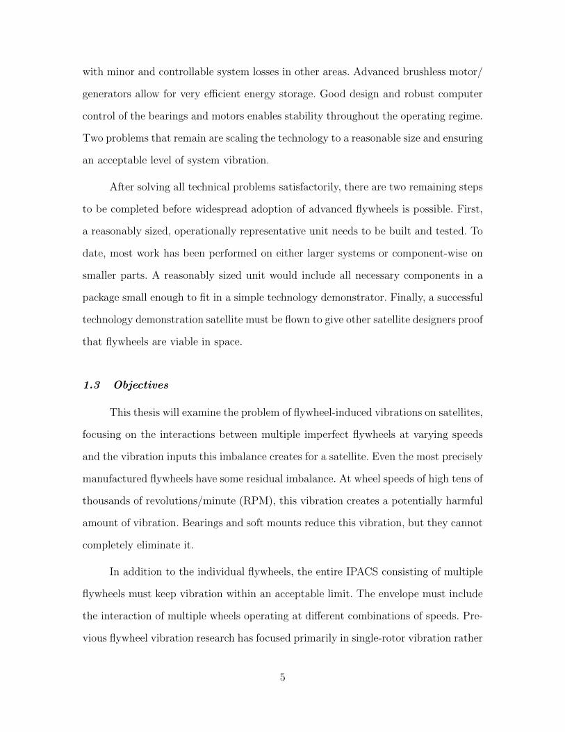
In September of 2004, NASA successfully tested the G2 flywheel module to a
speed of 41,000 RPM. G2 is shown in Figure 2 (9:132). Later that month, the same
team placed two flywheel modules (the older D1 and the newer G2) on an air bear-
ing table to demonstrate a full IPACS capability. They succeeded in demonstrating
controllable torque up to ±0.8 N-m and power transfer from 0–300 W. This was a
first for high-power, high-speed IPACS. Since then, however, active efforts towards a
flight-worthy technology demonstration have remained stalled.
With more recent technology advances, some researchers are beginning to de-
sign small IPACS for small satellites with demanding mission profiles. Lappas et al.
discussed this in an article that appears to be the most recent comprehensive review
of IPACS history and literature (12).
The control algorithms for IPACS have been studied very thoroughly, with many
papers written about both energy/power storage and attitude control. Two types of
10
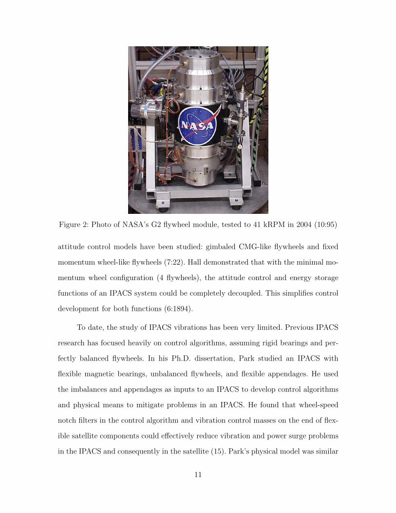
Figure 2: Photo of NASA’s G2 flywheel module, tested to 41 kRPM in 2004 (10:95)
attitude control models have been studied: gimbaled CMG-like flywheels and fixed
momentum wheel-like flywheels (7:22). Hall demonstrated that with the minimal mo-
mentum wheel configuration (4 flywheels), the attitude control and energy storage
functions of an IPACS system could be completely decoupled. This simplifies control
development for both functions (6:1894).
To date, the study of IPACS vibrations has been very limited. Previous IPACS
research has focused heavily on control algorithms, assuming rigid bearings and per-
fectly balanced flywheels. In his Ph.D. dissertation, Park studied an IPACS with
flexible magnetic bearings, unbalanced flywheels, and flexible appendages. He used
the imbalances and appendages as inputs to an IPACS to develop control algorithms
and physical means to mitigate problems in an IPACS. He found that wheel-speed
notch filters in the control algorithm and vibration control masses on the end of flex-
ible satellite components could effectively reduce vibration and power surge problems
in the IPACS and consequently in the satellite (15). Park’s physical model was similar
11

to the one developed in this thesis, but this thesis investigates instead the interactions
of vibrations between multiple flywheels.
The beat frequency has been studied briefly in rotordynamics. Research per-
formed at the Naval Postgraduate School used the beat frequency as a tuning aid to
match filter frequencies to vibration frequencies (13). The equations of motion for a
rigid body gyroscope are linear, however, and since the beat frequency’s effects on
a linear system are small as shown in Section 2.3.6, there has not been much study
of the effects of beat frequency in flywheel systems. One exception is a NASA in-
vestigation on beat frequency effects caused by pulse width modulation of position
sensor signals for a magnetically suspended flywheel rotor, but this model dealt with
non-linear effects rather than linear physical behavior (11).
While IPACS vibration has been largely neglected, the study of a single fly-
wheel’s vibration is completely within the realm of rotordynamics, which is very well
studied and is applicable to a wide variety of modern mechanical systems. Vance’s
Rotordynamics of Turbomachinery is one of the early comprehensive books on the sub-
ject (22:iv). Research in the field of rotordynamics is ongoing, and with the advent of
realizable controlled magnetic bearings, the state of the art continues to advance.
IPACS research has been ongoing for 50 years now, and no immediate demon-
stration is planned. The main obstacle in the way of a successful flight demonstration
is the complexity the problem—using an advanced and dynamic system to perform
two unrelated tasks. While many of these complications have been studied and some
of them have been mitigated, the vibration interactions between multiple flywheels in
one IPACS have been neglected. This thesis seeks to provide a look into the problem
of vibration interaction in order to determine whether it will be a problem for IPACS
in space. To peform this study, a flexible dynamics model is developed that will enable
research into vibrations of multiple gyroscope systems.
12

2.2 Coordinates and Nomenclature
There are two types of coordinates used in this model: wheel-aligned and global.
Both coordinate frames are right-handed in x, y, and z, with corresponding rotations
θx, θy, and θz.
The wheel-aligned coordinates are oriented such that the z axis is along the
flywheel spin axis for the wheel in question. The spin axis always points away from
the support structure, which is the system center of mass (COM). The x and y axes
are arbitrary in this coordinate frame since all inputs and outputs are cyclical in
nature about z. All discussions of individual flywheels refer to these local coordinates,
including all imbalance-induced input forces and wheel speeds.
The global coordinates are arranged with z “up”. This coordinate frame is
arbitrarily aligned. All system level references—including all response plots shown in
this thesis—will use the global coordinate system. Model inputs are applied internally
in the global frame. Coordinate systems are arranged as shown in Figure 3.
θxy
z
θz
θyx
(a) Global Coordinates
θxy
z
θz
θyx
(b) Wheel-aligned Coordinates
Figure 3: Coordinate systems used in this thesis
Nomenclature is defined as it is introduced, as well as appearing in a nomen-
clature section at the beginning of this thesis. A few terms are potentially confusing,
so a preview of them is in order here. Rotation angles θx,y,z are defined as shown in
13

Figure 3. θ is the vector of rotational states
([θx θy θz
]T), which are rotations
about x, y, and z, respectively. In the discussion of flywheels and rotors, wheel rota-
tion and speed are of particular importance, so θ with no letter subscript will refer to
the rotation angle of a rotor. Similarly, ω with no letter subscript will refer to rotor
speed, which would otherwise be referred to as θz.
Furthermore, there are three sets of units in widespread use to describe rota-
tional speed: rad/s, RPM, and Hz or revolutions/second (RPS). Flywheel dynamics
must be calculated in radians, but discussion is more intuitive in units of Hz or
RPS. Finally, system-level discussions of high-speed advanced flywheels commonly
uses units of RPM. The model developed in this thesis uses units of radians and
rad/s internally, but most discussion of wheel speeds in this paper will be in terms of
Hz and RPS.
2.3 Fundamental Equations
Understanding of several basic sets of equations is required for the study of
flywheel motion. A quick overview of some of these concepts is provided here.
2.3.1 Equation of Motion for a Gyroscopic Body. In this model, flywheels are
modeled as gyroscopic rigid bodies. The equation of motion (EOM) for a gyroscopic
rigid body is shown in matrix form in Equation 1 (18:124). Equation 1 also describes
the equation of motion for a non-spinning rigid body since gyroscopic stiffness, G, is
a function of wheel speed, ω, and it is zero for a non-spinning body.
Mq(t) + (C + G (ω(t))) q(t) + Kq(t) = u(t) (1)
14

where the state vector q =
[rT θT
]Tis composed of r = [x y z]
T and θ =
[θx θy θz]T, u is a vector of input forces, M is the mass matrix described in terms
of body mass m and directional MOI Ix,y,z. If the body is represented as a point
mass, M is the diagonal matrix M = diag
([m m m Ix Iy Iz
]). K and C are
the stiffness and damping matrices between the body and external nodes, and, when
described in wheel-aligned coordinates, G is the sparse skew-symmetric gyroscopic
matrix shown below.
G =
. . ....
0 −Izω 0
. . . Izω 0 0
0 0 0
.
In the simple case of a single body connected by springs to a fixed support,
stiffness would be written as K = −diag
([kx ky kz κθx κθy κθz
])with trans-
lational and rotational stiffnesses k and κ, respectively. Likewise, damping of a single
body would be described by C = −diag
([cx cy cz Cθx Cθy Cθz
])with trans-
lational and rotational damping of c and C.
In this model, however, the bodies will be connected not to fixed supports, but
to each other. Proper modeling of this inter-body stiffness requires the use of different
(and more complicated) stiffness and damping terms. These inter-body stiffness and
damping terms are only applicable to a system rather than to individual rigid bodies,
and they will be discussed in Section 3.3.1.
2.3.2 State-Space Equation of Motion. State-space representation is a con-
venient format for writing and solving linear differential equations, and it is the form
that will be used for the model in this thesis. In general, a linear system can be
15

described in state-space according to Equation 2 (17:210). Note that the notational
dependence on time is dropped for convenience.
q = Aq + Bu (2)
where A is the state matrix that describes system behavior and B is an input matrix
linking input forces to states.
Equation 3 below shows Equation 1, the gyroscopic EOM, in state-space form
with the addition of an input matrix, B. Note that the entire matrix EOM is found in
the second half of this equation; the top half is simply a computational convenience.
=
0 I
M−1K M−1(C + G)
+
0
M−1B
u (3)
2.3.3 Rotated Equation of Motion. If the flywheel EOM is known in the
wheel-aligned coordinate frame, but the integration is to be carried out in a different
global coordinate frame, Equation 3 must be rotated accordingly. Recalling that the
entire matrix EOM is found in the second half of the state-space equation, the correct
application of the rotation matrix R is shown below in Equation 4. Proper rotation is
required when a collection of bodies with different local coordinate frames is integrated
into one state-space system.
=
I 0
0 R
0 I
M−1K M−1(C + G)
I 0
0 RT
+
0
RM−1BRT
u (4)
16

2.3.4 Centripetal Force. The primary input in this model will be the vibra-
tion caused by an unbalanced spinning flywheel rotor, which is a centripetal force.
Equations 5 and 6 show the equations for centripetal acceleration, ac, and its associ-
ated force, fc in polar coordinates (1:75–76).
ac = −ρω2 (5)
fc = −eω2 = −mρω2 (6)
where eccentricity e represents rotor mass m and the distance between the flywheel’s
COM and the center of the shaft, ρ. Wheel speed is again represented by ω. The
distance ρ is shown in Figure 4. The vectors e and ρ point from the center of mass
to the flywheel shaft.
ρ
Figure 4: A spinning flywheel of mass m with COM–shaft distance ρ creates a cen-tripetal input force proportional to eccentricity e = mρ
2.3.5 Natural Frequencies of a Rotor/Bearing System. The IPACS model in
this thesis will be used to evaluate vibration interactions. One potentially troublesome
vibration is resonant frequency excitation of the flywheels. Rigid rotors have several
17

vibration modes, and those are briefly explained here. In this brief discussion of natural
frequencies, ω1–ω4 will refer to natural frequencies of the rotor/bearing system, and
ω with no subscripts will refer to wheel speed.
When a rigid rotor is restrained in the x and y directions by springs of stiffness
K as shown in Figure 5, the EOM from Equation 1 can be simplified to the forms
shown below in Equations 7–10.
mx+ 2kx = 0 (7)
my + 2ky = 0 (8)
IT θx + IPωθy +1
2kL2θx = 0 (9)
IT θy − IPωθx +1
2kL2θy = 0 (10)
where m = rotor mass, L = rotor length, and It and Ip are the transverse and polar
MOIs, respectively (22:125).
The natural frequencies, ωn, of the rigid body rotor/bearing system shown in
Figure 5 and described in Equations 7–10 are shown in Equations 11–13. Recall that
ω represents angular rotor speed.
ω1 = ω2 =
√2K
m(11)
ω3(ω) =IP2IT
ω +
√KL2
2IT+
(IP2IT
ω
)2
(12)
ω4(ω) =IP2IT
ω −
√KL2
2IT+
(IP2IT
ω
)2
(13)
Natural frequencies ω1 and ω2 correspond to translational vibration modes in
the x and y directions. Frequencies ω3 and ω4 correspond to the forward and backward
18
θx y
zθz
θyx
k k
kk
L
ω
Figure 5: A long rigid rotor constrained by springs in x and y
whirling modes, respectively. Whirling is a precession-like motion. Forward whirl (ω3)
is rotation in the same direction as wheel spin, as shown in Figure 6. Backward whirl
(ω4) is rotation in the opposite direction.
Modes 1 and 2 are constant and identical. They represent “bouncing” in the
x and y directions. There is no angular motion associated with these modes. The
frequency of these modes is solely a function of bearing stiffness and rotor mass.
Modes 3 and 4 are, respectively, the speed-dependent forward and backward
conical whirling motions. With a wheel speed of zero, ω3(0) = ω4(0) = ωT =√
KL2
2IT,
which is the natural rigid body pitching/yawing frequency. Rigid body vibration at
this frequency will be simple pitching or yawing about θx or θy.
As rotor speed, ω, increases, the pitching and yawing motions become whirling
motions, and the frequencies of the forward and backward whirls diverge from ωT , with
forward whirl speed increasing and backward whirl speed decreaseing. As wheel speed
approaches infinity, ω3 approaches P and ω4 approaches 0. P is the ratio IP/IT (polar
19

ω z
x y
z
Figure 6: Depiction of forward whirling motion
MOI/transverse MOI), which represents rotor configuration. For a short coin-like disc
or hoop, P = 2. For an infinitely long rotor, P = 0 (22:126).
Figure 7 shows the normalized natural frequencies of the forward and backward
whirl modes, respectively. Recall that ωT , the natural rigid body pitching/yawing
frequency is√
KL2
2IT. Backward whirl has a negative frequency value because it is
in the direction opposite wheel spin. These modes are dependent on P , the rotor
configuration (22:127).
Of the whirl modes, ω3 is the mode most easily excited by rotor imbalance.
Figure 7(a) shows that short rotors are not self-exciting for forward whirl, but long
rotors have a critical coning frequency where the wheel frequency is synchronous with
the whirl frequency. The critical coning frequency, ωcon is found by setting ω ≡ ω3 in
Equation 12, resulting in Equation 14.
ωcon =
√ω2T
1 − P(14)
20

0 0.5 1 1.5 2 2.5 3 3.5 4 4.5 50
1
2
3
4
5
6
Wheel Speed (ω / ωT)
Whi
rl S
peed
(ω3 /
ωT)
P = 0.1P = 0.5P = 1P = 2synchronous
(a) Forward Whirl (ω3)
0 0.5 1 1.5 2 2.5 3 3.5 4 4.5 5
−1
−0.9
−0.8
−0.7
−0.6
−0.5
−0.4
−0.3
−0.2
−0.1
0
Wheel Speed (ω / ωT)
Whi
rl S
peed
(ω4 /
ωT)
P = 0.1P = 0.5P = 1P = 2
(b) Backward Whirl (ω4)
Figure 7: Normalized whirl modes for various flywheel rotor configurations. Dottedline for forward whirl shows where whirl speed is synchronous with wheelspeed. Natural rigid-body pitching frequency ωT is used to normalize plotsfor all rotor/bearing configurations (22:128)
21

Operation near the critical coning frequency can be unstable, although momen-
tarily passing through this region is acceptable, allowing operation in supercritical
regions (21:354). For long rotors (P < 1), this critical frequency must be kept low
enough to be out of the operating range of the rotor. Shorter rotors (P > 1) do not
have this problem, but an outside excitation at the coning frequency could be haz-
ardous. Outside excitation at critical coning frequencies is examined in this paper for
both short and long rotors, which are the sub- and super-synchronous rotor frequency
problems.
Natural frequencies ωn as found in Equations 11–13 are described in units of
rad/s. For the remainder of this thesis, natural frequencies will be instead described
in units of Hz as fn, where
fn =ωn2π
(15)
This terminology will eliminate any confusion between wheel speeds (described as ω)
and the natural frequencies.
2.3.6 Beat Frequency. For linear systems, the response of a system to two
inputs can be found by adding the system’s response to the individual inputs. This
superposition can yield a stronger or weaker response than either signal individually,
depending on whether the sum of the responses is positive or negative, creating either
constructive or destructive interference.
When waveforms of two frequencies (ω1, ω2) differ in frequency by a small
amount δ, (ω2 = ω1 + δ), the wave which results from their combination will exhibit
what is known as a beat phenomenon due to alternating constructive and destructive
22

interference. Using the relationship
sinA+ sinB = 2 sinA+B
2cos
A− Y
2,
the sum (y1 + y2) of two displacements
y1 = sinω1t
y2 = sinω2t = sin (ω1 + δ)t
can be written as shown in Equation 16 (16:23).
y = y1 + y2 = 2 sin
(ω1 +
δ
2
)t cos
(δ
2
)t (16)
Figure 8 shows an example of a beat frequency created by the superposition of
two waves with similar frequencies. The resultant waveform is a sine wave of frequency
ω = ω1+ω2
2which is shaped by the envelope described by ±2 cos
(δ2
)t. This envelope
has a much lower frequency than either of the original waves.
When two signals are combined in a linear system they are superimposed addi-
tively. In order to see system excitation at the beat frequency, there would have to be
some non-linear process allowing the input frequencies to be multiplied. Otherwise,
there will be no change in frequency. This lack of excitation at the beat frequency
should manifest itself in a lack of energy at the beat frequency in a power spectral
density (PSD) plot. The signal shown in Figure 8 was analyzed with the Matlab®
pwelch command to create the PSD plot shown in Figure 9.
As expected, Figure 9 shows that the signal in Figure 8 has energy at both input
frequencies, but there is no system energy at the beat frequency of 5 Hz. In linear
23

0 0.1 0.2 0.3 0.4 0.5 0.6 0.7 0.8 0.9 1−2
−1.5
−1
−0.5
0
0.5
1
1.5
2
time (sec)
y = y1+y2
2cos(δ t/2)
Figure 8: Beat phenomenon created by inputs of frequency 30 and 35 Hz
0 10 20 30 40 50 60−80
−70
−60
−50
−40
−30
−20
−10
0
10
Frequency (Hz)
Pow
er/fr
eque
ncy
(dB
/Hz)
Figure 9: Power spectral density plot of the signal shown in Figure 8. Note the lackof energy at the beat frequency of 5 Hz
24

systems there should be no excitation at this beat frequency, even if some connected
structure has a natural frequency close to the beat frequency.
2.4 Model
The model used in this thesis represents two advanced flywheels mounted to
a support structure and nominally spinning in opposite directions. The rotors are
mounted with active magnetic bearings, and their operating speed range is 20,000–
60,000 RPM (333–1000 RPS). They are powered by high-efficiency motor/generators.
The rotors nominally spin at the same speed to store energy, changing speed relative
to each other to control the attitude of the satellite.
2.5 Scope
The model developed in this thesis relies on several assumptions to limit the
scope of the analysis. The only source of vibration studied is rotor imbalance. There
are multiple other real sources of vibration including torque ripple, sensor error, band-
width limitations, and external vibrations. These additional vibration sources are ig-
nored.
Also, this model does not take into consideration any motion of the satellite.
In a satellite with an IPACS, the satellite body will be free to rotate, and can be
controlled by the varying rotation rates of the flywheels. In the model used in this
thesis, the IPACS is subjected mainly to symmetric or periodic disturbing forces from
a static equilibrium state, and it does not experience large rotations. When necessary,
a spring is used to enforce small angles. The spring constraint makes the use of small
angle approximations for IPACS rotation appropriate and allows for a simpler linear
analysis. Similarly, this model does not account for any rotor translation along or
rotation about the axis of the flywheel, except that the gyroscopic stiffness increases
25

with increasing rotor speed. The bearings in this model are assumed to be linear
springs, as opposed to the controllable magnetic bearings of an actual IPACS.
Even the best control model will be unable to completely filter out all dis-
turbances such as rotor imbalance due to limitations such as signal bandwidth and
control saturation. This model assumes a small residual amount of rotor imbalance
that cannot be filtered out and examines the interactions between multiple residual
imbalances. Therefore, the input and output forces are small.
The scope of this analysis is also limited to rigid flywheel rotors. There are
higher bending modes associated with flexible rotors, but the first four vibration
modes discussed in Section 2.3.5 are dominant—bending modes are typically above a
frequency of 1 kHz (15:35).
26

III. Methodology
3.1 Overview
This thesis will use an analytical model to study the vibration interaction of
multiple gyroscopes. Vibrations can come from several sources, but this thesis will
examine only those caused by unbalanced flywheels. The model will be numerically
integrated using the ode45 command in Matlab®.
3.2 Model Description
3.2.1 Model Construction. The model used in this thesis is a system of two
flywheels and a support structure as shown in Figure 10. The flywheels are axially
aligned, with opposite spin directions. The flywheels are arranged such that the system
COM and the support COM are co-located.
ω
ω
x,θx y,θy
z,θz
Figure 10: Basic configuration of the model used in this thesis
The flywheels are each connected to the support structure with two magnetic
bearings, as shown in Figure 11. Flywheels of length l and radius r are located at
distance d from the support COM and supported at each end by a magnetic bearing.
The magnetic bearings have only translational stiffness, but having one of them at
27

each end of the rotor will create an effective rotational stiffness. The stiffnesses in
the transverse (x and y) and axial (z) directions are separate and not necessarily
related. In this thesis, however, axial displacements are ignored, so the axial stiffness
is unimportant. When damping is accounted for in this thesis, all springs shown
represent bearings with both stiffness and damping.
d
r
x,θ y,θ
z,θ
yx
z
l
Figure 11: Flywheel in housing connected to IPACS support structure
The model is simplified by replacing each body with a point mass as shown
in Figure 12. There is one 4 degree of freedom (DOF) spring (and damper) located
at the flywheel’s COM, which is attached to the support structure with a rigid link.
The spring shown has transverse translational (x and y) and rotational (θx and θy)
stiffness.
For a flywheel of length l with individual magnetic bearing stiffness kmag, the
model will have linear stiffness kmodel = 2kmag and transverse rotational stiffness
κT,model = 12kmagl
2 (22:125). Damping is similar: cmodel = 2cmag and CT,model = 12cmagl
2.
28

: wheel
: support
d
i
j
y,θ
z,θ
y
z
Figure 12: Model of support/flywheel connection. Bodies are point masses separatedby distance d
The two flywheels are attached to the support structure as discussed previously
and illustrated again in Figure 13. Also shown is a connection to the satellite, which
represents a soft mount between the support structure and the rest of the satellite.
Since all forces studied are periodic or symmetric about the system and support struc-
ture COM, the support will primarily experience rotations rather than translations.
For this reason, the satellite/support spring is modeled as a 3 DOF spring with only
rotational stiffness. The satellite in this model is assumed to be heavy enough that
it can be considered fixed. For most validation runs, the satellite/support spring was
turned off to allow free rotation of the satellite.
Finally, an appendage can be added to the model. The appendage represents a
flexible spacecraft structure such as a solar array or antenna, and it is used to study
low frequency excitation. The appendage is shown in Figure 14. The appendage and
support structure COMs are co-located, and they are connected by a 2 DOF spring
with only transverse (θx and θy) rotational stiffness.
3.2.2 Model Inputs. The sources of vibration in this model will be rotor
imbalances. Real rotors can have very small imbalances if they are manufactured
29

ω
IPACSsupport
4 DOF
4 DOF
1
ω2
3 DOF
x,θ y,θ
z,θ
yx
z
(x,y,θx,θy)
(x,y,θx,θy)
(θx,θy,θz)
satellite(fixed)
Figure 13: System model with satellite included. The satellite/support spring can beturned off if needed
x,θ y,θ
z,θ
yx
z
Figure 14: Model of appendage, which is connected to the support structure with onlya rotational spring
30

with tight tolerances, but imbalances will always be present after manufacturing. The
rotors in this model will be assumed to be imbalanced in such a way that they cause
a purely two-dimensional vibration: linear (in x, y) or rotational (in θx, θy). These
imbalances are shown conceptually in Figure 15. The axially symmetric imbalances
in a real rigid rotor can be described as a combination of these two imbalances, but
they will be examined individually in this model.
x,θ y,θ
z,θ
yx
z
(a) Linear (b) Rotational
Figure 15: Two sources of axially-symmetric imbalance-induced vibration
The rotating imbalance creates a centripetal force as discussed in Section 2.3.4.
For this model the rotor eccentricities are replaced with an ideal rotor plus periodic
input forces synchronized with wheel position and proportional to eccentricity and
the square of the wheel speed.
3.2.3 Model Parameters. The flywheel for this model is a theoretical flywheel
only, but it is intended to be realistically sized. Flywheel parameters are given in
Table 1.
Magnetic bearing stiffness and damping are similar to those used in some NASA
studies (4). The nominal mass properties are described in Hibbeler’s text (8). They
are defined here in such a way that they describe a short rotor(P = IT
IP> 1)
to study
super-synchronous whirl. When necessary, IT is changed to adjust the rotor parameter
31

Table 1: Flywheel model parameters
mag bearing stiffness kmag 1756 kN/mmag bearing damping cmag 3.512 kN/m/srotor mass m 10 kgrotor length l 20 cmsupport/rotor distance d 15 cmrotor radius r 15 cmrotor shaft/COM distance ρ 0.01 nmmodel translational stiffness kmodel 3512 kN/mmodel rotational stiffness κmodel 35.12 kN-m/radmodel translational damping cmodel 7.024 kN/m/smodel rotational damping Cmodel 70.24 N-m/rad/stransverse MOI IT 0.0896 kg-m2
polar MOI IP 0.1125 kg-m2
rotor MOI ratio P 1.2558 -
P . This adjustment is made to study longer rotors when looking for sub-synchronous
whirl. The COM–shaft offset distance, ρ was chosen to give similar disturbance inputs
to the residual disturbances found by Park (15:87). The mass properties of the support
structure are shown in Table 2.
Table 2: Support structure parameters
mass m 10 kgMOI Ix,y,z 10 kg-m2
3.3 System Equation of Motion
3.3.1 System Equation of Motion Components. When a system of indepen-
dent, unconnected, gyroscopic rigid bodies is described in state-space as shown in
Equation 2, it takes the form of the block diagonal matrix shown in Equation 17.
The stiffness and damping terms here represent each body being connected to a fixed
body.
32

q =
A1 . . . 0
.... . .
...
0 . . . An
q +
B1
...
Bn
u (17)
where the state vector q =
[q1
T . . . qnT
]T, qi =
[ri
T θiT vi
T ωiT
]T, and Ai
and Bi are defined according to Equations 18 and 19, similar to Equation 4. ri and
θi are the position (x, y, z) and rotation (θx, θy, θz) vectors of the bodies, respectively,
and vi and ωi are the corresponding translational and rotational velocities.
Ai =
[Ri
] 0 I
M−1i Ki M−1
i (Ci + Gi)
[RTi
](18)
Bi =
[Ri
] 0
M−1i Bi
[RTi
](19)
A system of connected rigid bodies is described by the same equation of motion
given in Equation 17 plus the addition of non-block diagonal stiffness terms in the
A matrix. In the case of this model, the stiffness between each flywheel and the
support structure is identical in the local axially aligned frame. This common stiffness
matrix can be derived using the spring equation with the help of a diagram of system
displacements. With the support and the wheel modeled as point masses, a simple
diagram of displacements in x is shown in Figure 16, which is a simplification of the
housing support structure. Small angles are assumed.
Figure 16 is used to determine the inter-body spring forces caused by system
displacements according to F = −kx. The bodies are modeled as point masses. Angles
33

xj*=xi +θy,id
xj xi
θy,i
θy,j
z,θ
x,θx
z
: wheelj
: supporti
d
Figure 16: System displacements in x. Bodies i and j are point masses. This diagramis used to determine spring forces between bodies i and j in the x direction.The flywheel (j) is attached to the end of a rigid link length d extendingfrom the support structure (i)
are assumed to be small, so sin θ ≈ θ and cos θ ≈ 1. x∗j describes the displacement of
the rotor support structure in the x direction. The rotor’s position in x is defined as
xj. The x direction resultant spring force on mass i due to the displacements shown
in Figure 16 is given below in Equation 20.
ΣFx = −kx(xi + θy,id− xj) (20)
Simlarly, the resultant torques on mass i about the y axis are described below
in Equation 21.
ΣTy = −κy(θy,i − θy,j) − kd(θy,id+ xi − xj) (21)
34

The remaining resultant forces and torques on mass i can be determined by
analogy or by the construction of a similar diagram. The forces and torques on mass i
in y and θx are shown below in Equation 22. Since this model ignores rotor motion in
z and θz, those equations are not listed.
ΣFy = −ky(yi − θx,id− yj) (22)
ΣTx = −κx(θx,i − θx,j) − kd(θx,id− yi + yj)
Likewise, the forces acting on mass j (the flywheel) are shown below in Equa-
tion 23.
ΣFx = −kx(xj − xi − θy,id) (23)
ΣFy = −ky(yj − yi + θx,id)
ΣTx = −κx(θx,j − θx,i)
ΣTy = −κy(θy,j − θy,i)
Equations 20–23 can be represented in matrix form as shown in Equation 24
where i, j are the bodies being connected. They describe the forces applied to the
bodies by various system displacements.
f if j
=
Ki,i Ki,j
Kj,i Kj,j
qiqj
(24)
35
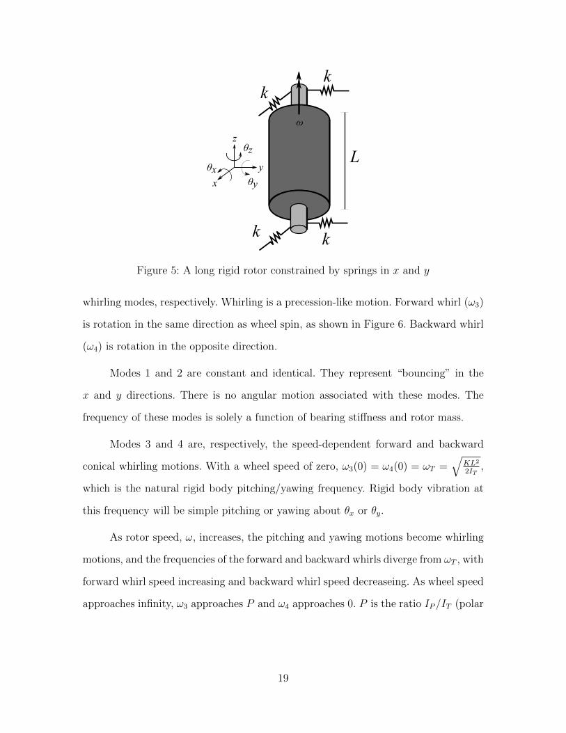
Ki,i =
−kT 0 0 0 −kTd 0
0 −kT 0 kTd 0 0
0 0 0 0 0 0
0 kTd 0 −kTd2 − κT 0 0
−kTd 0 0 0 −kTd2 − κT 0
0 0 0 0 0 0
Ki,j =
kT 0 0 0 0 0
0 kT 0 0 0 0
0 0 0 0 0 0
0 −kTd 0 κT 0 0
kTd 0 0 0 κT 0
0 0 0 0 0 0
Kj,i = KT
m,n
Kj,j =
−kT 0 0 0 0 0
0 −kT 0 0 0 0
0 0 0 0 0 0
0 0 0 −κT 0 0
0 0 0 0 −κT 0
0 0 0 0 0 0
For this model, mass i is always the support structure, so i ≡ 1. This 12 x 12
stiffness matrix is separated into four parts which are placed into the global system
A matrix in the appropriate locations.
36

The damping matrix, C, is treated the same way. This model uses damping
proportional to stiffness to represent the losses in the system. This is represented by
C = ξK, where ξ = 0.002, which is reflected by the values in Table 1.
3.3.2 System Equation of Motion Assembly. Recalling Equations 2 and 17,
a state-space system EOM is written as
q = Aq + Bu
Both A and B are assembled from their component parts, which are described
in Section 3.3.1. This can also be represented as shown in Equations 25 and 26.
A = M−1system (AG + AK + AC) (25)
B = M−1systemBsystem (26)
where
M−1system =
I 0
0 M−11
. . .
I 0
0 M−1n
37

AG =
0 I
0 G1
. . .
0 I
0 Gn
AK =
0 0 0 0 0 0
ΣK1,1 0 K1,2 0 K1,n 0
0 0 0 0 0 0
K2,1 0 ΣK2,2 0 K2,n 0
. . .
0 0 0 0 0 0
Kn,1 0 Kn,2 0 ΣKn,n 0
AC =
0 0 0 0 0 0
0 ΣC1,1 0 C1,2 0 C1,n
0 0 0 0 0 0
0 C2,1 0 ΣC2,2 0 C2,n
. . .
0 0 0 0 0 0
0 Cn,1 0 Cn,2 0 ΣCn,n
38

Subscripts on stiffness and damping terms are the i, j subscripts found in Equa-
tion 24. Placement of each term is determined from Equation 18. AK and AC of
Equation 25 are more general than the model requires. Since the only connections
in the model are between body 1 (the support structure) and other bodies, many of
the terms shown in these general equations are unnecessary, leading to the simplifi-
cation of AK as AK∗ as shown below, where all of the off-diagonal terms not along
the first row or column are zero. AC∗ is similar. The stiffness term for the support
structure, ΣK1,1, also contains the stiffness between the fixed satellite bus and the
support structure.
AK∗ =
0 0 0 0 0 0
ΣK1,1 0 K1,2 0 K1,n 0
0 0 0 0 0 0
K2,1 0 K2,2 0 0 0
. . .
0 0 0 0 0 0
Kn,1 0 0 0 Kn,n 0
The input matrix B is simpler. It links each of the states with an input un. The
column and row of a B term determine which input force is applied to which state,
respectively. Because the EOM is represented in the second half of each body’s state
vector, that is where the inputs are applied.
39
Bsystem =
0
B1
...
0
Bn
(27)
This model incorporates rotating centripetal force inputs synchronized to the
rotation of each flywheel. The input vector describing each of these terms is shown in
Equation 28.
u =
[e1ω
21 sin θ1t e1ω
21 cos θ1t . . . enω
2n sin θnt enω
2n cos θnt 1
]T(28)
As Equation 28 shows, the input vector has two centripetal force terms for each
wheel, and they are 90◦ out of phase from each other. The magnitude of the force is
eiω2i , and the force acts in the direction of the current wheel rotation, θi. In the model
this is divided into x and y (or θx and θy) inputs, which vary periodically with sin θi
and cos θi. The last term, 1, is used to allow for a constant force input for validation
purposes. This vector is used for all model input. Different system input cases are
created by applying forces (imbalances or a constant force) to various states with
changes in the input matrix B.
3.4 Integration
The model created in Matlab® is integrated numerically using ode45. The
differential equation created by the state-space model is kept as small as possible
because it must be integrated over many iterations. Some components of the system
40

EOM, however, are functions of time. Both the gyroscopic matrix G and the force
vector u are time dependent and they must be recomputed for each iteration of the
integration.
In addition, careful attention must be paid to the application of rotating input
forces. A periodic rotating input force is represented in two linear dimensions as a sine
wave in one dimension and a cosine wave in the other dimension. If these forces are
directly applied to an unconstrained mass initially at rest, they can cause a secular
drift in one direction. This phenomenon occurs in the model used for this thesis (but
not the actual system). One solution to minimize the effect of the secular drift is
described in Appendix A.
3.5 Additional Components
3.5.1 Appendage. The addition of a flexible appendage is accommodated by
adding another body to the model. An appendage is used to study the beat phe-
nomenon as it applies to this model. Since the studied effects of this appendage are
limited to θx and θy, the appendage is only connected to the model with torsional
springs. Also, the only relevant mass properties are Ix and Iy. These properties, which
were chosen to give the appendage a natural frequency of 5 Hz, are shown in Table 3.
Table 3: Appendage mass properties
mass Ix,y 10 kg-m2
transverse MOI κT 9869 N-m/rad
In the model, the appendage is added as a new body with mass Mapp =
diag
([1 1 1 10 10 1
])and stiffness Kapp defined according to Equation 24,
with all terms except κT
41

3.5.2 Satellite/support spring. When required, a spring is connected between
a firm fixed satellite and the support structure. Since input forces are cyclical and
cause primarily rotations in the support structure, it is the rotational DOFs that be-
come problematic and require constraints. This additional spring is attached to K1,1,
as discussed in Section 3.3.2, and takes the form Ksupport = −1×10⁶diag
([0 0 0 1 1 0
]).
3.6 Validation
3.6.1 Validation Inputs. A simple IPACS model was created for validation
purposes. The flywheel properties for this model are shown in Table 4. This model
has a long rotor, so it will have a critical coning speed.
Table 4: Validation model flywheel properties
rotor mass m 10 kgrotor length l 0.5 mrotor radius r 0.12 msupport/rotor distance d 1 mmag bearing stiffness kmag 2500 N/mpolar MOI IP 0.0781 kg-m2
transverse MOI IT 0.2474 kg-m2
rotor MOI ratio P 0.3158
For validation, several test inputs were given to the model and the responses
were verified. First, a few constant-direction forces were applied to ensure that signs
were correct and that the model components were assembled correctly. Exponential
rotational growth due to a constant applied torque is shown in Figure 17. Figure 17
and all similar figures show a time history of each system displacement for each wheel.
All responses are shown in global coordinates.
The next set of tests were performed to ensure the model’s consistency in ac-
counting for wheel spin direction. One wheel at a time was given an imbalance input
42

0 0.1 0.2−1
0
1
x(m
)
Support
0 0.1 0.2−5
0
5x 10
−21
y(m
)
0 0.1 0.20
5x 10
−4
θ x(r
ad)
0 0.1 0.2−1
0
1
θ y(r
ad)
time (s)
0 0.1 0.2−1
0
1wheel 1
0 0.1 0.2
−4
−2
0x 10
−4
0 0.1 0.20
5x 10
−4
0 0.1 0.2−1
0
1
time (s)
0 0.1 0.2−1
0
1wheel 2
0 0.1 0.20
5x 10
−4
0 0.1 0.20
5x 10
−4
0 0.1 0.2−1
0
1
time (s)
(a) Wheel speed: 0 (b) Input force: asshown
Figure 17: System demonstrating exponential displacement growth due to a constanttorque input applied to θx
43
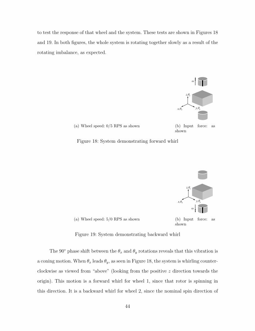
to test the response of that wheel and the system. These tests are shown in Figures 18
and 19. In both figures, the whole system is rotating together slowly as a result of the
rotating imbalance, as expected.
(a) Wheel speed: 0/5 RPS as shown
ω
x,θ y,θ
z,θ
yx
z
(b) Input force: asshown
Figure 18: System demonstrating forward whirl
(a) Wheel speed: 5/0 RPS as shown
ω
x,θ y,θ
z,θ
yx
z
(b) Input force: asshown
Figure 19: System demonstrating backward whirl
The 90◦ phase shift between the θx and θy rotations reveals that this vibration is
a coning motion. When θx leads θy, as seen in Figure 18, the system is whirling counter-
clockwise as viewed from “above” (looking from the positive z direction towards the
origin). This motion is a forward whirl for wheel 1, since that rotor is spinning in
this direction. It is a backward whirl for wheel 2, since the nominal spin direction of
44

rotor 2 is opposite that of wheel 1. When θy leads θx, the system is rotating in the
opposite direction and the whirl orientations are reversed. This response was studied
with the normal system model, not the validation model.
Next the system’s natural frequencies were examined. The first three natural
frequencies of a rotor-bearing system are given in Equations 11–13 and 15. Recall that
f1 = f2 are bouncing modes, and f3 and f4 are forward and backward whirling modes.
The system responses demonstrating f1–f4 are shown in Figures 20–24. Figure 20
demonstrates the bouncing mode f1 = f2.
0 0.5 1−1
0
1
x(m
)
Support
0 0.5 10
0.01
0.02
y(m
)
0 0.5 1−5
0
5x 10
−18
θ x(r
ad)
0 0.5 1−1
0
1
θ y(r
ad)
time (s)
0 0.5 1−1
0
1wheel 1
0 0.5 10
0.005
0.01
0 0.5 1−5
0
5x 10
−18
0 0.5 1−1
0
1
time (s)
0 0.5 1−1
0
1wheel 2
0 0.5 10
0.005
0.01
0 0.5 1−5
0
5x 10
−18
0 0.5 1−1
0
1
time (s)
(a) Wheel speed: zero
y,θy
z,θz
(b) Initial state:as shown
Figure 20: System demonstrating bouncing vibration at f1 ≈ 6.16 Hz
Equation 11 gives the natural frequency of a spring-mass system as f1 =√k/m/2π.
The model’s two flywheels were displaced symmetrically to make the system equiv-
alent to a free two-body system. The equivalent mass of a freely vibrating two-body
system can be found by meq =(∑n
i=1m−1i
)−1. With a 10 kg support structure and
two 10 kg flywheels, the system equivalent mass is 6.66 kg and f1 = f2 ≈ 6.16 Hz.
45

Figure 21 shows the expected forward and backward whirl speeds of the valida-
tion model. By inspection, when wheel speed is zero, f3 = f4 ≈ 5.66 Hz, which agrees
with Equation 12. At a wheel speed of 10 RPS, f3 ≈ 7.36 Hz and f4 ≈ 4.40 Hz.
0 2 4 6 8 10 120
2
4
6
8
10
12
wheel speed (Hz)
whi
rl sp
eed
(Hz)
f3−f4
Figure 21: Whirl modes of the validation system. Dotted line is synchronous withwheel speed
Figure 22 shows that the forward whirl mode behaves as expected with flywheel
speed ω = 0. Backward whirl at this speed is identical except for direction, which
appears as an opposite phase difference in θx and θy.
The whirl modes are dependent on wheel speed and they diverge with increasing
wheel speed. Figures 23 and 24 show the whirl modes when wheel speed is 10 RPS.
f3(10 Hz) ≈ 7.36 Hz and f4(10 Hz) ≈ 4.40 Hz. In both cases the system whirl is in
the same direction (counter-clockwise as viewed from “above”), but the wheel speed
directions were changed as necessary to make these forward or backward whirling
motions.
46

0 0.5 1−0.01
0
0.01
θ x(r
ad)
wheel 1
0 0.5 1−0.5
0
0.5
θ x(r
ad/s
)
0 0.5 1−0.02
0
0.02
θ y(r
ad)
0 0.5 1−0.5
0
0.5
θ y(r
ad/s
)
time (s)
0 0.5 1−0.01
0
0.01wheel 2
0 0.5 1−0.5
0
0.5
0 0.5 1−0.02
0
0.02
0 0.5 1−0.5
0
0.5
time (s)
(a) Wheel speed: 0
x,θx y,θy
z,θz
(b) Initial state: asshown
Figure 22: Forward whirl with zero wheel speed: f3 = f4 ≈ 5.66 Hz. Backward whirlis identical except for direction
0 0.5 1−0.01
0
0.01
θ x(r
ad)
wheel 1
0 0.5 1−0.5
0
0.5
θ x(r
ad/s
)
0 0.5 1−0.01
0
0.01
θ y(r
ad)
0 0.5 1−0.5
0
0.5
θ y(r
ad/s
)
time (s)
0 0.5 1−0.01
0
0.01wheel 2
0 0.5 1−0.5
0
0.5
0 0.5 1−0.01
0
0.01
0 0.5 1−0.5
0
0.5
time (s)
(a) Wheel speed: 10 RPS as shown
ω
ω
x,θx y,θy
z,θz
(b) Initial state: asshown
Figure 23: Forward whirl mode at f3 ≈ 7.36 Hz when wheel speed is 10 RPS
47

0 0.5 1−0.02
0
0.02
θ x(r
ad)
wheel 1
0 0.5 1−0.5
0
0.5
θ x(r
ad/s
)
0 0.5 1−0.02
0
0.02
θ y(r
ad)
0 0.5 1−0.5
0
0.5
θ y(r
ad/s
)
time (s)
0 0.5 1−0.02
0
0.02wheel 2
0 0.5 1−0.5
0
0.5
0 0.5 1−0.02
0
0.02
0 0.5 1−0.5
0
0.5
time (s)
(a) Wheel speed: 10 RPS as shown
ω
ω
x,θx y,θy
z,θz
(b) Initial state: asshown
Figure 24: Backward whirl mode at f4 ≈ 4.40 Hz when wheel speed is 10 RPS
Forward whirl f3 is speed dependent and, for a long rotor, there is a critical con-
ing speed where the whirling frequency is the same as the wheel frequency. Figure 25
demonstrates this phenomenon. Wheel speed is varied from 4–12 RPS, and vibration
is much worse at the critical coning frequency fcon ≈ 6.8 Hz. The difference between
the support structure’s vibration in θx and θy is a modeling artifact.
3.7 Summary
The model developed for this thesis was tested and performed correctly given a
variety of input scenarios, including initial conditions, constant forces, and periodic
forces. Critical coning frequency was demonstrated successfully, as well as forward
and backward whirls.
48

Figure 25: Model demonstrating the critical coning frequency. As the wheel speedpasses through fcon ≈ 6.8 Hz, the vibration amplitude gets much larger.Wheel speed varies linearly from 4 RPS at t=4 to 12 RPS at t=12
49

IV. Results and Analysis
Several tests were conducted using the model described in this thesis, and the results
are presented here. First, a full frequency sweep was performed to see if any imme-
diate problems arose. Other tests examined the existence of beat phenomenon and
extra-synchronous whirl excitation. For this section, flywheel-specific rotation speed
is represented as ωn.
4.1 Full Envelope Sweep
First a variety of full envelope frequency sweep tests were carried out. For these
tests, wheel speed of one or both rotors varied from 333–1000 RPS. A moment-
inducing imbalance in each rotor caused a vibration input synchronized with each
wheel speed.
These tests revealed nothing of interest except that the system’s gyroscopic
stiffness diminishes as the wheel speeds approach equality in opposite directions. This
reduction in gyroscopic stiffness is illustrated nicely in Figures 26–28.
x 10x 10x 10
Figure 26: System rotations as a result of moment-inducing imbalance vibrations.Wheel speeds: ω1 = 333, ω2 = 333–1000 RPS
50
Figure 27: System rotations as a result of moment-inducing imbalance vibrations.Wheel speeds: Wheel speeds: ω1 = 1000, ω2 = 333–1000 RPS
Figure 28: System rotations as a result of moment-inducing imbalance vibrations.Wheel speeds: ω1 = 1000–333, ω2 = 333–1000 RPS
51

The system response clearly changes frequency in each case. The time-varying
long-period wobble in the system is caused by the sudden application of the input
forces, which causes a slight misalignment between the angular momentum vector
and the flywheel rotation axes. The system angular momentum vector gets larger as
the flywheel speeds get further apart, giving the system as a whole more gyroscopic
stiffness. The additional stiffness manifests in an increased oscillatory frequency and
a smaller displacement from the equilibrium state as expected.
In all cases, the vibration-inducing imbalance forces are less significant than the
system’s slow oscillation. The magnitude of the imbalance-induced vibration is evi-
denced by the thickness of the lines seen in Figures 26–28. A closer look at the rotation
of the support structure as shown in Figure 29 reveals that the wheel-synchronous
vibration is small relative to the long-period oscillation. This figure shows the same
data seen in Figure 26.
Adding a flexible appendage (representing a satellite structure such as an an-
tenna or solar array) to the system does not change the response very much. Figure 30
shows the response of the system’s flexible appendage, which has a natural frequency
of 5 Hz. There is some vibration evident at the natural frequency of the appendage,
but the response is dominated by the slow oscillation of the support structure.
The slow, changing oscillation seen in Figures 26–30 accurately reflects the re-
sponse of a system with changing gyroscopic stiffness given an initial whirling type
motion. The initial whirling motion seen in these figures, however, is an artifact of
modeling, caused by the instant application of a disturbing force. Such a motion is
possible and indeed uncontrollable in a two wheel IPACS, but it can only be caused
by an external disturbance force. In an IPACS with full 3-axis control authority, the
control in other dimensions would be used to eliminate the whirling motion.
52

Figure 29: A closer look at the support structure vibration from Figure 26. This viewshows the wheel-synchronous vibration
Figure 30: A closer look at the appendage vibration from Figure 26. This view revealsa small amount of vibration at the appendage’s natural frequency, butbehavior is dominated by long-period oscillation
53

4.2 Beat Frequency Analysis
After studying the effect of near-frequency input vibrations, it is evident that
this model does not reveal any beat frequency problems. This is unsurprising given
the linear nature of the model.
The flexible appendage did experience a small resonant vibration when the
difference of two input frequencies matched the natural frequency of the appendage,
but it experienced the same vibration with other unrelated input frequencies.
First, the two-wheel model was run with slightly different wheel speeds: 333 and
338 RPS. The 5 RPS difference in the wheel speeds creates a beat frequency which
matches the natural frequency of the flexible appendage, which was not yet added.
As Figure 31 shows, the 5 Hz beat frequency is clearly evident.
Figure 31: Beat frequency is clearly visible in the support structure when ω1 =333, ω2 = 338 RPS
Next the model was run at the same wheel speeds with the flexible appendage
added. The appendage represents a flexible satellite body such as a solar panel or
antenna. The rotational state history from this test is shown in Figure 32. The beat
frequency is still clearly visible, and the appendage is experiencing vibration near its
natural frequency.
54

x 10
Figure 32: Beat frequency is still visible in the support structure when ω1 = 333, ω2 =338 RPS, and the appendage experiences excitation at its resonant fre-quency of 5 Hz
Finally, the same model with flexible appendages was run with a new and wider
wheel speed difference: ω1 = 333, ω2 = 400 RPS. This is shown in Figure 33. The
beat frequency is no longer present, but the appendage still exhibits vibration near its
natural frequency. The vibration magnitude of the appendage in this figure is largely
the same as seen in Figure 32.
x 10
Figure 33: Beat frequency is gone, but appendage still vibrates near its resonant fre-quency of 5 Hz when ω1 = 333, ω2 = 400 RPS
From studying the results of the tests performed with both frequency offsets,
it appears that there is no more low frequency excitation at the difference frequency
of two inputs than there is at any other combination of inputs. The beat frequency
55

exists, but its effects are very limited. Recalling Equation 16, the combined output of
two signals that are close in frequency can be written as
y = 2 sin
(ω1 +
δ
2
)t cos
(δ
2
)t
The maximum magnitude of the resultant vibrations shown in Figure 31 should
be twice that of the vibrations evident when only one source of vibration is present.
To check this, a test was run with only one wheel spinning. Figure 34 shows that
the vibration magnitude is indeed approximately half of the peak seen when a beat
frequency is present.
Figure 34: Vibration here, caused by one wheel rotating at 333 RPS, is approximatelyhalf the peak vibration seen in Figure 31
A power spectral density plot of the support structure’s vibrations during beat
frequency and non-beat frequency conditions reveals that there is no power at the
low beat frequency. During the beat case, wheel speeds are: ω1 = 333, ω2 = 338 RPS.
For the non-beat case, the speed of wheel 2 is raised to ω2 = 400 RPS. The peak-
normalized PSD of both responses is shown in Figure 35.
The PSD reveals that there is no energy at the low beat frequency, and the
rotation time histories reveal that there is no extraneous excitation as a result of
the beat frequency. Aside from periodically doubling the magnitude of the resultant
56

Figure 35: Peak-normalized PSD of support structure θx during beat (ω1 = 333, ω2 =338 RPS) and non-beat (ω1 = 333, ω2 = 400 RPS) conditions. Low fre-quency response is nearly identical. Note peaks at the input excitationfrequencies
57

high-frequency vibration, there is no negative effect from the beat phenomenon in a
linear system.
4.3 Extra-Synchronous Whirl Excitation
Long rotors have a critical coning frequency, fcon where the wheel speed is
synchronous with the forward whirl speed. This was illustrated with Figure 25 in Sec-
tion 3.6.1. All rotors, however, have forward and backward whirl modes. With multi-
ple flywheels in one system, the flywheels provide each other with extra-synchronous
vibration sources, and it may be possible for these extra-synchronous frequencies
to excite unexpected resonances. Both sub- and super-synchronous excitations were
studied for this phenomenon.
In this section, ω refers to flywheel-specific wheel speed. Forward and backward
whirl speed are respectively referred to as f3 and f4, which were derived and explained
in Section 2.3.5. Spectrograms are used in this section to illustrate the time-varying
nature of the response frequencies. All spectrograms are derived from θx (the rotation
about x) of the wheel in question. Units are very small and are included only for the
purpose of comparison between different cases. The satellite/support spring was used
for all of the tests in this section.
4.3.1 Sub-Synchronous Whirl Excitation. A long-rotor model was used to
look for sub-synchronous whirl excitation. Sub-synchronous resonance is vibration
of a long rotor at speeds lower than the wheel speed. Sub-synchronous resonance
is at a higher frequency than the critical coning frequency, fcon, where the forward
whirl frequency crosses the wheel frequency. The region of interest using the flywheel
parameters chosen for this study is seen in Figure 36, which shows both the forward
and backward whirl of the long rotor used in this study.
58

0 100 200 300 400 500 600 700−100
0
100
200
300
400
500
600
700
wheel speed (RPS)
whi
rl fr
eque
ncy
(Hz)
f3f4
Figure 36: Forward and backward whirl modes of the sub-synchronous study model
In the sub-synchronous test, the wheels will spin at two different speeds. The
vibration input of the slower wheel should excite a forward whirling mode in the faster
wheel, even if the faster wheel is perfectly balanced.
The flywheel parameters used for this study are shown in Table 5. Other param-
eters remain the same as those shown in Table 1 from Section 3.2.3. This model was
studied both with and without bearing damping included. These values were chosen
not for realism, but to give favorable conditions for excited whirl at a frequency other
than the wheel frequency.
Table 5: Flywheel parameters for sub-synchronous study
mass m 10 kgpolar MOI IP 0.1125 kg-m2
transverse MOI IT 0.2015 kg-m2
rotor MOI ratio P 0.5583
59

In the sub-synchronous test, wheel 2 was perfectly balanced and operated at
700 RPS. This gives it a forward whirl frequency of f3 ≈ 400 Hz and a backward
whirl frequency of f4 ≈ −11 Hz. Wheel 1 was given a moment-inducing imbalance
and operated at speeds intended to excite f3 of the faster balanced wheel, or about
400 RPS. Wheel 1’s own speed, ω1 caused separate whirling frequencies in wheel 1:
f3 ≈ 242 Hz and f4 ≈ −18 Hz. Natural frequencies can be found by inspection from
Figure 36 and analytically with Equations 12 and 13 from Section 3.2.3. In all cases
the speed of wheel 1 (the unbalanced excitation wheel) varies from 350 RPS at t = 0
to 450 RPS at t = 2.
4.3.1.1 Undamped sub-synchronous response. At first, damping was
neglected to see if there would be any response. Wheel 1’s response is shown in
Figure 37. Note the strength of the self-induced, sub-synchronous, forward whirling
mode. This wheel is well past its critical coning speed for forward whirl, but it is
still responding strongly at the whirling frequency. In fact, at lower wheel speeds the
resonant forward whirling response is stronger than the input disturbance.
400
x,θ y,θ
z,θ
yx
z
700
Figure 37: Spectrogram of wheel 1’s response to its own undamped imbalance. ω1
varies from 350–450 RPS. Note the strong forward whirling resonance
60
Wheel 2’s response over the same time period was examined at multiple speeds.
Figure 38 shows the wheel 1 response at a baseline of ω1 = 0 and at ω = ∓700 RPS.
Wheel 2 experienced a significant forward whirling motion when it was rotating in
the same direction as wheel 1. Support response in all cases was similar.
Two spurious vibrations can be found in Figure 38. Most notable is the constant
frequency vibration at approximately 50 Hz which appears in 38(a) and 38(c). The
50 Hz vibration appears to be worse when the excitation is at 400 Hz, but it is actually
worse at approximately 1 sec, and occurs repeatedly if the integration time is longer.
There is also a vibration at approximately 70 Hz visible in 38(a). These vibrations do
not match either of the rotor’s resonant frequencies, and they are system level effects
caused by the bus/support springs and the net gyroscopic stiffness.
Two notable vibrations do appear, however. The first of these vibrations is at
the backward whirl frequency, f4, of wheel 1 (the excitation wheel). This vibration at
approximately 20 Hz is visible in all three scenarios of Figure 38, but is strongest in
the response shown in Figure 38(c), which is the case where the wheels are spinning in
opposite directions. This excitation indicates that wheel 1 is exciting its own backward
whirl mode through interaction with wheel 2, even though wheel 2 is perfectly balanced.
The other vibration apparent in Figure 38 is the vibration that appears near
t = 1 second at approximately 400 Hz in 38(b). This frequency is the forward whirl
speed of wheel 2, and the intended excitation frequency of this test model. This vibra-
tion appears and is most severe about halfway through the test, when the excitation
frequency is 400 Hz. Forward whirl in wheel 2 is expected to be worst at that time
because it is being excited at f3. The persistence of the whirling motion after the
excitation frequency has moved past the resonant frequency shows that whirl tends
to persist after excitation. The same time history appeared when wheel 1’s speed was
61

400
x,θ y,θ
z,θ
yx
z
(a) ω2 = 0
400
x,θ y,θ
z,θ
yx
z
700
(b) ω2 = -700 RPS
400
x,θ y,θ
z,θ
yx
z
700
(c) ω2 = 700 RPS
Figure 38: Spectrogram of wheel 2’s response to sub-synchronous vibration input.ω1 varies from 350–450 RPS. Note the different frequency scale in subfig-ure (b). Vibration at 50 Hz fades in and out repeatedly
62

varied backwards, from 450–350 RPS. In other words, the appearance and decrescendo
of a whirling motion was consistent in time, not in input frequency.
Note that the model configuration represented in 38(b) is not operationally
realistic for a two wheel IPACS, but it demonstrates sub-synchronous excitation. The
problem is that both wheels are spinning in the same direction, which does not allow
for high power storage and transfer with a net zero angular momentum change. In
reality, the wheels will be spinning in opposite directions as they are for the case
shown in Figure 38(c). This situation might occur, however, in a bank of multiple
rotors, such as one being used primarily for energy storage.
4.3.1.2 Damped sub-synchronous response. Since sub-synchronous ex-
citation was found to affect a two flywheel system with no damping, the next step
was to see if it remained when damping was included in the model. The same test
conditions used in the undamped case were used to study a more realistic damped
flywheel configuration.
Figure 39 shows the response of wheel 1, the excitation wheel. Note that the
resonant whirling response has been attenuated below the threshold of visibility in
this spectrogram and all that remains is the synchronous imbalance-induced vibration.
Since the wheel speed is so far from the critical whirling frequency fcon, even the very
small amount of damping present in this model is enough to eliminate this resonance.
Figure 40 shows the damped response of wheel 2 to the same sub-synchronous
imbalance input that induced forward and backward whirl in the undamped case. All
resonances have fallen below the detectable threshold, leaving only the direct input
frequency created by the unbalanced rotation of wheel 1.
From the significant and beneficial effect of even modest damping in this multiple
flywheel IPACS model, it appears that real flywheel systems are safe from the harmful
63

400
x,θ y,θ
z,θ
yx
z
700
Figure 39: Spectrogram of wheel 1’s response to its own damped imbalance. ω1 variesfrom 350–450 RPS. The forward whirling resonance is gone
effects of sub-synchronous flywheel vibration in an axially opposed configuration.
Real flywheels necessarily include damping since it is a real and unavoidable physical
phenomenon.
4.3.2 Super-synchronous Whirl Excitation. A short-rotor model with the
nominal parameters given in Table 1 from Section 3.2.3 was used to look for super-
synchronous whirl excitation. Super-synchronous resonance is vibration of a short
rotor at speeds higher than the wheel speed. Ordinarily this is not a problem for short
rotors, since their forward whirling frequencies always remain higher than the wheel
speed. An external vibration input at the resonant speed could induce vibration in
this mode, however. Figure 41 shows the forward and backward whirling frequencies,
f3 and f4, for this configuration.
This test used the same setup as the test for sub-synchronous whirl, with dif-
ferent rotors and a different excitation speed. In this test wheel 1 was spun from
950–1050 RPS in an attempt to excite vibration modes in wheel 2, which was spin-
ning at ∓700 RPS. A non-spinning wheel was again used as a baseline. Whirl modes
64

400
x,θ y,θ
z,θ
yx
z
700
(a) ω2 = -700 RPS
400
x,θ y,θ
z,θ
yx
z
700
(b) ω2 = 700 RPS
Figure 40: Wheel 2 damped sub-synchronous spectrograms. ω1 varies in time from350–450 RPS. Frequencies other than the input have been attenuated
65

0 100 200 300 400 500 600 700 800 900 1000 1100−200
0
200
400
600
800
1000
1200
1400
wheel speed (RPS)
whi
rl fr
eque
ncy
(Hz)
f3f4
Figure 41: Forward and backward whirl modes of the super-synchronous study model.One dotted line is zero and the other is synchronous with the wheel speed.
for wheel 2 are f3 ≈ 890 Hz and f4 ≈ −12 Hz. For wheel 1, f4 ≈ −7.9 Hz. f3 for
wheel 1 is well above any vibrations present in the system, since the rotors are short.
Damping was again at first neglected to see if there would be a response. The
super-synchronous excitation response was very similar to the sub-synchronous excita-
tion response. Spectrograms in this section show a wheel 1 speed range from 850 RPS
at t = 0 to 950 RPS at t = 2.
Spectrograms of the wheel 1 and support responses did not reveal any reso-
nances. The only place in the model with any visible extra-synchronous frequency
response was wheel 2. The spectrograms for wheel 2 are shown in Figure 42. Simi-
lar to the sub-synchronous case, there is a slight forward whirl response when spin
directions are identical, and there is a slight backward whirl excitation regardless of
relative spin directions.
66

900
x,θ y,θ
z,θ
yx
z
(a) ω2 = 0
900
x,θ y,θ
z,θ
yx
z
700
(b) ω2 = -700 RPS
900
x,θ y,θ
z,θ
yx
z
700
(c) ω2 = 700 RPS
Figure 42: Spectrograms of wheel 2’s undamped response to super-synchronous vi-bration input. ω1 varies in time from 850–950 RPS
67

Figure 42 also reveals a slight response around the backward whirl modes. There
is not enough spectral resolution in the figures to determine which wheel’s response
is causing the vibration. They are very close in frequency, however (approximately 8
and 12 Hz), and perhaps both of them are responding.
As seen in Figure 43, resonant vibrations due to a super-synchronous vibration
excitation disappear when damping is included in the model, similar to the disap-
pearance of resonant vibration in the sub-synchronous test.
4.4 Summary
The model developed in this thesis was used to investigate potential causes of
troublesome low frequency vibration in an IPACS. Beat frequency was found to have
absolutely no impact on low frequency vibrations, and minimal impact at any fre-
quency, with the only impact being the periodic doubling of the input forces. Extra-
synchronous resonance excitation, both sub- and super-synchronous, was found to
have only a small impact on satellite vibrations. Backward whirl was excited regard-
less of spin directions, but extra-synchronous forward whirl was only excited when
spin directions were identical. Extra-synchronous vibration is very small relative to
the inducing imbalance, but it is at a lower frequency. The identical spin direction
configuration is of no concern for a simple IPACS, but could be a factor in a bank
of flywheels intended primarily for energy storage. With a small amount of damping,
however, all extra-synchronous vibration effects disappear.
68

900
x,θ y,θ
z,θ
yx
z
(a) ω2 = 0
900
x,θ y,θ
z,θ
yx
z
700
(b) ω2 = -700 RPS
900
x,θ y,θ
z,θ
yx
z
700
(c) ω2 = 700 RPS
Figure 43: Spectrograms of wheel 2’s damped response to super-synchronous vibrationinput. ω1 varies in time from 850–950 RPS
69

V. Conclusion
5.1 Summary
In this thesis a flexible linear dynamics model was developed to study vibra-
tions in a system of multiple connected gyroscopic flywheels. The model was validated
through several types of test input, and then used to analyze various sources of vibra-
tion interaction between two flywheels a simulated IPACS. System parameters were
intended to be representative of a near-future technology demonstration mission to
validate the use of flywheels for energy storage and attitude control in space.
The source of vibration studied in this model was an assumed eccentricity caused
by manufacturing defect. Furthermore, it was assumed that this defect was attenuated
by active magnetic bearing control methods described in previous literature. The
residual vibrations after attenuation were used as model inputs. The vibration inputs
were applied in the radial and transverse directions to an axially-aligned two-flywheel
IPACS.
The model was then used to study interactions between multiple sources of
vibration in an IPACS. Specifically, the beat frequency and extra-synchronous vibra-
tion excitation phenomena were studied, including both sub- and super-synchronous
vibration excitation scenarios.
5.2 Findings
The beat frequency problem was shown to have almost no impact in a linear
system. The extra-synchronous vibration effects were both found to have a small effect
on a double flywheel system. When mild damping was applied, effects were below the
threshold of observability, but with no damping there was a small but consistent
system response to backward whirl modes. In addition, if there are multiple flywheels
70

with the same spin direction, extra-synchronous forward whirl in one wheel can be
excited by another unbalanced wheel.
Of the vibration sources considered in this thesis, extra-synchronous resonance
excitation, both sub- and super-synchronous, proved to be of some potential concern
in the future development of IPACS. As bearing and flywheel system technology con-
tinues to improve, damping will continue to fall as flywheel designers seek to remove
sources of loss from their systems. At some point the damping may be small enough
to allow the extra-synchronous resonances to affect the system negatively. Vibrations
caused by input interactions are much smaller than the vibrations themselves, but
they are also at a lower frequency.
Park proposed a notch filter centered at the wheel speed to mitigate the effects of
wheel imbalance to an IPACS or satellite. If bearing development produces magnetic
bearings with low enough damping to allow the extra-synchronous resonant vibration
to become a problem, the control system designer could also develop methods for
mitigating extra-synchronous vibration modes.
5.3 Contributions
This thesis proved the existence of inter-flywheel vibration interactions in a
multiple flywheel system. Extra-synchronous resonance excitation between multiple
rotors was found to exist in an ideal undamped configuration, but even a very small
realistic amount of damping was enough to mitigate the effect to the point that it
was less of a concern than individual rotor vibration inputs.
5.4 Recommendations for Future Work
This thesis showed that damping can mitigate and possibly eliminate unde-
sirable extra-synchronous flywheel vibration. Future research should be done to de-
71

termine how low the bearing damping can be before the sub-synchronous resonance
negatively affects system operation.
In addition, the model developed in this thesis was used to investigate some of
the effects of multiple flywheel vibrations in an IPACS, but this thesis was limited
in scope to analyzing two co-axial rotors with simple imbalance-induced vibrations
in and about 2 axes. In an advanced flywheel there is also significant potential for
rotational vibration about the spin axis due to torque ripple. In the co-axial case the
torsional vibrations will remain independent from other system disturbances, but in
a flywheel system with multiple non-co-axial rotors, torsional vibrations will induce
other vibrations that may be deleterious to successful IPACS implementation on a
satellite.
The analysis of those extra factors should be undertaken as a further step along
the path to developing flywheel energy storage systems. With torsional stiffness turned
on and the appropriate input forces applied, the model developed in this thesis is
capable of performing this evaluation.
Furthermore, as flywheel performance continues to improve and bearing de-
velopment produces magnetic bearings with lower losses, the vibration interaction
effects uncovered in this thesis may become significant. If that occurs, flywheel bear-
ing controllers must be able to account for and mitigate the effects of backward whirl
excitation between flywheels.
5.5 Conclusion
Flywheels may someday be a key component for providing the satellite designer
with flexibility and performance benefits. Their successful on-orbit deployment has
to this point been delayed longer than any of the original proponents of the idea
could have envisioned, and many problems in this area remain unstudied. Someday,
72

however, enough problems will be solved to make flywheels in orbit a viable reality.
The engineering community must continue to work diligently in this area until that
day arrives.
73

Appendix A. One Integration Problem and a Solution
Position is the double integration of acceleration, which is proportional to the input
force as shown in Equation 29.
x(t) =
∫v(t) =
∫∫a(t) =
∫∫f(t)
m(29)
Given sinusoidal inputs acting on a 1 kg mass:
f(t) = sin t cos t
a(t) = sin t cos t
v(t) = − cos t+ c1 sin t+ c1
x(t) = − sin t+ c1t+ c2 − cos t+ c1t+ c2
If the mass is initially at rest (x0 = v0 = a0 = 0), the constants are found to be:
f(t) = sin t cos t
c1 = 1 0
c2 = 0 1
When a sine wave force is applied to an unconstrained mass initially at rest,
c1 will cause a positive secular drift. This drift does not occur if the input force is
a cosine wave. The difference between sine and cosine input forces is illustrated in
Figure 44.
The drift illustrated in Figure 44 is a phenomenon observed only in modeling;
it does not occur in real systems. Most models do not reveal the drift because they
model systems constrained by some spring force. For unconstrained systems, a model
can reveal a drift, but it does not exist in reality because the periodic rotating forces
74

0
0
Sine
Acc
eler
atio
n
00
Vel
ocity
00
Pos
ition
Time
0
0
Cosine
0
0
00
Time
Figure 44: Acceleration, velocity, and position due to sinusoidal inputs applied to afree body initially at rest
such as wheel imbalances always grow from an initial magnitude of zero. It is only a
factor when modeling a system that is rotating at t = 0.
Because the rotating force must be represented as a sine wave in one dimension,
the direct application of this force will cause a secular drift. One solution is to delay
the application of this force until the input force has rotated 90◦. This delay will cause
the sine wave to look like a cosine wave (it will begin from 1 rather than from 0),
and it will be shifted correctly in phase. With multiple input forces, each one must
be “turned on” at the appropriate moment. Given the numerical nature of the model
in this thesis, the limits of integration must match these times as well to ensure that
the sine input is applied at exactly the right moment. “Turning on” the forces at the
correct times will eliminate this source of drift.
75

Appendix B. Matlab® Code
Listing B.1: ../models/model.m1 function [output] = model (config)
2 global ss model input output c ii model
3 % Feb 2011
4 % Jordan Firth
5
6 % state = [x y z a b g x’ y’ z’ a’ b’ g’]’
7
8 %% constants
9 % compute/import data from case_maker
10 [model ,input] = case_reader(config );
11
12 %% R Matrices
13 % r3- each page of array is rot mat for one wheel
14 % r12 - blkdiag of 4 r*3’s- rotate all 4 states of the wheel at once
15
16 % R- one giant rotation matrix for the whole massive A matrix -may not need
17
18 % Here are the rz ’s
19 r3 = zeros(3,3,model.nwheels ); % preallocate for speed
20 r12 = zeros (12,12, model.nwheels ); % preallocate for speed
21 R = zeros(model.nwheels *12); % preallocate for speed
22 for i = 1: model.nwheels
23 r3(:,:,i) = Rmaker1(model.zps(:,i)); % r3 is ind. rot. matrix
24 %blkdiagn creates super -duper 4x rot. matrix (x..a..dx..da..)
25 r12(:,:,i) = blkdiagn(r3(:,:,i),4); % stores all r12 ’s in array
26 R(12*i -11:12*i, 12*i -11:12*i) = r12(:,:,i); % giant rotation matrix
27 end
28
29 %% mi’s- mass matrix inverses
30
31 % compute M inverses once and store for speed
32 mbusi6 = model.msupport ^-1;
33
34 mi6 = model.mwheel ^-1;
35 mi12 = blkdiag(eye(6), mi6);
36
37 % mi for dummy mass
38 if model.dummy
39 mdummyi6 = model.mdummy ^-1;
40 end
41
42 %% A Matrix
43 % Create a-matrices and assemble into A
44
45 ss.A_rb = blkdiagn ([zeros (6) eye (6); zeros (6,12)], model.nwheels );
46
47 % % these are useful sometimes when the model breaks
48 % size(rz12 (:,:,1))
49 % size(blkdiag(Mbusi6 ,Mi6))
50 % size(k)
51
52 % K and C terms
53 for i = 2: model.nwheels
54
55 % K
56 K = r12(:,:,i) * blkdiag(mbusi6 ,mi6) * model.k * r12(:,:,i)’;
57 ss.A_rb (7:12 ,1:6) = ss.A_rb (7:12 ,1:6) + K(1:6 ,1:6);
58 ss.A_rb (7:12 ,12*i -11:12*i-6) = ss.A_rb (7:12 ,12*i -11:12*i-6) + K(1:6 ,7:12);
59 ss.A_rb (12*i -5:12*i ,1:6) = ss.A_rb (12*i -5:12*i,1:6) + K(7:12 ,1:6);
60 ss.A_rb (12*i -5:12*i,12*i -11:12*i-6) = ss.A_rb (12*i -5:12*i,12*i -11:12*i-6) + ...
61 K(7:12 ,7:12);
62
63 % C
76

64 C = r12(:,:,i) * blkdiag(mbusi6 ,mi6) * model.c * r12(:,:,i)’;
65 ss.A_rb (7:12 ,7:12) = ss.A_rb (7:12 ,7:12) + C(1:6 ,1:6);
66 ss.A_rb (7:12 ,12*i -5:12*i) = ss.A_rb (7:12 ,12*i -5:12*i) + C(1:6 ,7:12);
67 ss.A_rb (12*i -5:12*i ,7:12) = ss.A_rb (12*i -5:12*i ,7:12) + C(7:12 ,1:6);
68 ss.A_rb (12*i -5:12*i,12*i -5:12*i) = ss.A_rb (12*i -5:12*i,12*i -5:12*i) + ...
69 C(7:12 ,7:12);
70 end
71
72 ss.A_rb (7:12 ,1:6) = ss.A_rb (7:12 ,1:6) + mbusi6 * model.busk;
73
74 % here is my dummy mass for vibe
75 if model.dummy
76 x=model.nwheels *12+1;
77 a = [zeros (6) eye(6) ; mdummyi6*model.kdummy (7:12 ,7:12) zeros (6)];
78 ss.A_rb = blkdiag(ss.A_rb ,a);
79
80 ss.A_rb (7:12 ,1:6) = ss.A_rb (7:12 ,1:6) + mbusi6*model.kdummy (1:6 ,1:6);
81 ss.A_rb (7:12,x:x+5) = ss.A_rb (7:12 ,x:x+5) + mbusi6*model.kdummy (1:6 ,7:12);
82 ss.A_rb(x+6:x+11 ,1:6) =ss.A_rb(x+6:x+11 ,1:6) + mdummyi6*model.kdummy (7:12 ,1:6);
83 clear a
84
85 input.q0 = [input.q0; zeros (12 ,1)];
86 end
87
88 %% B Matrix
89
90 ss.B = zeros (12* model.nwheels ,model.nwheels ); % preallocate for speed
91 clear a
92 for ii = 2:model.nwheels;
93 a = zeros (12 ,2);
94 a([7 10] ,1) = input.b([7 10],ii);
95 a([8 11] ,2) = input.b([8 11],ii);
96
97 ss.B(12*ii -11:12*ii ,2*ii -1:2*ii) = r12(:,:,ii) * mi12 * a;
98 end
99 clear a
100
101 % input.b1 creates constant direction input forces (just for testing)
102 input.b1 = mi12*input.b1;
103 input.b1 = input.b1(:);
104 ss.B = [ss.B input.b1];
105
106 %% W matrices
107 % these will actually be created in the solver , but I do as much work here
108 % as possible to save integration time
109
110 % W
111 % stretch vector: mathworks.com/matlabcentral/newsreader/view_thread /129069
112
113 input.w_(1,:) = input.w(1 ,:);
114 input.w_(2,:) = (input.w(2,:)-input.w(1 ,:))/( input.time);
115
116 a = repmat(input.w_(1,:),12,1);
117 b = repmat(input.w_(2,:),12,1);
118
119 % input.w_ = input.w_ ’;
120
121 input.W(:,:,1) = diag(a(:));
122 input.W(:,:,2) = diag(b(:));
123 clear a b
124
125 %% G matrices
126 % these will actually be created in the solver , but I do as much work here
127 % as possible to save integration time
128 Ip = model.mwheel (6,6);
129 ss.G = zeros (12* model.nwheels );
77

130 for i = 2: model.nwheels
131 j = 12*i;
132 ss.G(j-2:j,j-2:j) = Ip * r3(:,:,i) * mi6 (4:6 ,4:6) * ...
133 [[0 -1 0];[1 0 0];[0 0 0]] * r3(:,:,i)’;
134 end
135
136 %% find integration times
137 % Each wheel must be integrated to and from the time when it crosses
138 % theta = pi/2. Here I find those times and create a time vector which
139 % contains the appropriate integration limits.
140
141 clear a b
142 a = [input.w_(2 ,:)/2; input.w_(1,:); -pi/2* ones(1,model.nwheels )]’;
143 b=[];
144 for ii = 1:model.nwheels
145 b = [b roots(a(ii ,:)) ’]; % only need the max time
146 end
147
148 % remove solutions outside of my time window (0-tf)
149 b=b(b>0);
150 b=b(b<input.time);
151
152 t = unique ([0 b input.time ]); % [0, intermediate times , tf]
153
154 clear a b
155
156 %% fix matrices for dummy mass
157 if model.dummy
158 ss.B = [ss.B; zeros(12,size(ss.B ,2))];
159 ss.G = blkdiag(ss.G,zeros (12));
160 x = model.nwheels *12;
161 input.W = cat(2,input.W,zeros(x,12 ,2));
162 input.W = cat(1,input.W,zeros(12,x+12 ,2));
163 clear x
164 end
165
166 %% solve equation
167 % run with state_space_model (no need to run the entire model 10000 times)
168
169 options = model.options;
170 output.t = [];
171 output.q = [];
172 for ii = 1: length(t) - 1
173 time = [t(ii) t(ii+1)-1E -80];
174 [output_t ,output_q] = ode45(@state_space_model ,time ,input.q0,options ,input ,ss);
175 output.t = [output.t; output_t ];
176 output.q = [output.q; output_q ];
177
178 input.q0 = output.q(size(output.q,1) ,:);
179 end;
180
181 end
182
183 function dq = state_space_model(t,q,input ,ss )
184 % global A q B u
185 % global peanut teakettle
186 % W(t) varies from w0 to wf - used to get correct gyro stiffness in A
187 W = input.W(:,:,1) + input.W(:,:,2) * t;
188
189
190 % vibe input has to look like a cosine (start from 1). If it looks like a
191 % sine , the position drifts. Since the circular force of the imbalance
192 % needs both sines and cosines , I have to include sines , but I accomplish
193 % it by not starting them until theta = pi/2
194
195 % this is where i determine theta
78
196 theta = (input.w_(1,:)*t + input.w_(2 ,:)/2*t^2);
197
198 % here is wheel speed at t=time
199 w = (input.w_(1,:) + input.w_(2,:)*t);
200 % peanut = [peanut w(2)]; see w while testing
201 % teakettle = [teakettle t]; see t while testing - to match up with w
202
203 % this is the magnitude of the centripetal force input
204 u_mag = input.e * w.^2;
205
206 % and here I test and only include the sine if theta >=pi/2
207 % sin/cos(theta) is direction; u_mag is magnitude
208 u = [cos(theta ).* u_mag; sin(theta ).* u_mag .*(abs(theta)>=pi/2)];
209
210 u = [u(:); 1];
211
212 B = ss.B;
213
214 A = ss.A_rb + W*ss.G;
215
216 dq = A*q + B*u;
217 end
Listing B.2: ../models/case reader.m1 function varargout = case_reader(file_num)
2 % clc;
3 % [model ,input] = case_reader(file_num)
4 % show = case_reader(file_num)
5 %
6 % when called with 2 output arguments , returns model and input , which are
7 % structures that contain everything model.m needs
8 % when called with 1 output argument , returns show (wheels and axes)
9
10 % check for correct number of arguments (1 or 2)
11 if nargout ~=1 && nargout ~=2; error(’something is horribly wrong’); end;
12
13 filename = [’cases/’ num2str(file_num) ’.txt’];
14
15 check = struct(’wheels ’,0,’axes’ ,0);
16 local.L = 0;
17
18 %% reads file only to find show - which wheels and axes to display
19 % show contains show.wheels and show.axes
20 if nargout == 1
21 fid = fopen(filename );
22 while ~feof(fid)
23 key = textscan(fid ,’%s’,1,’delimiter ’,’ ’);
24 value = textscan(fid ,’%s’,1,’delimiter ’,’\n’);
25 % char(key{1,1}) % for testing
26 switch char(key{1,1})
27 case ’wheels:’
28 if check.wheels; disp(’wheels multiply defined ’); end
29 show.wheels = str2num(cell2mat(value {:}));
30 check.wheels = 1;
31 case ’axes:’
32 if check.axes; disp(’axes multiply defined ’); end
33 show.axes = str2num(cell2mat(value {:}));
34 check.axes = 1;
35 otherwise
36 % do nothing
37 end
38 end
39 fclose(fid);
40 varargout (1) = {show};
41 return
79

42 end
43
44 %% nargout must be 2-> read file for model configuration
45 %% set up geometry of wheels (#, orientation)
46 % orientation of spin axis (wheel z) in global coords
47 model.zps = [[0 0 1]’ [0 0 1]’ [0 0 -1]’];
48
49 % # wheels derived from zps
50 model.nwheels = size(model.zps ,2);
51 %% set variables to defaults
52 model.busk = zeros (6); % no bus/support spring
53 model.dummy = 0; % no dummy mass (appendage)
54 % define dummy mass terms anyways , we ’ll just ignore them if dummy=0
55 model.mdummy = diag ([1 1 1 10 10 1]);
56 kdummy = 1000*pi^2* diag ([0 0 0 1 1 0]);%*1.23456;
57 model.kdummy = [-kdummy kdummy; kdummy -kdummy ];
58
59 input.w = zeros(2,model.nwheels ); % w = 0 for all wheels
60
61 % default is no initial input or state
62 qbuilder = zeros (12,( model.nwheels+model.dummy ));
63 input.b = qbuilder;
64 input.b1 = qbuilder;
65
66 % default integration time
67 input.time = 1;
68
69 % empty ode45 options
70 model.options = [];
71
72 %% read the case file and set up the model
73 fid = fopen(filename );
74 while ~feof(fid)
75 key = textscan(fid ,’%s’,1,’delimiter ’,’ \n’);
76 % char(key {:})
77 value = textscan(fid ,’%s’,1,’delimiter ’,’\n’);
78 value = cell2mat(value {: ,:});
79 switch char(key{1,1})
80 case ’config:’ % complete
81 % value {1,1} for testing
82 % config = value;
83 switch value
84 case ’validation ’
85 [k,c,mwheel ,msupport ,L] = validation_model;
86 case ’super’
87 [k,c,mwheel ,msupport ,L] = super_model;
88 case ’thesis ’
89 [k,c,mwheel ,msupport ,L] = super_model;
90 case ’sub’
91 [k,c,mwheel ,msupport ,L] = sub_model;
92 otherwise; error(’uh-oh’)
93 end
94 model.k=k; model.c=c; model.mwheel=mwheel; ...
95 model.msupport=msupport;
96 % local =setfield(local ,’L’,L);
97 local.L = L;
98 local.config = value;
99 case ’busk’ % complete
100 model.busk = -1e6*diag([0 0 0 1 1 0]);
101 case ’appendage ’ % complete
102 model.dummy = 1;
103 case ’time:’ % complete
104 input.time = str2num(value);
105 case ’whz:’ % complete
106 input.w = ones (2,3) .* str2num(value) * 2*pi;
107 case ’wrpm:’ % complete
80

108 input.w = str2num(value) * 2*pi /60;
109 case ’damping:’ % complete
110 % if str2num(cell2mat(value {:}))==0
111 % str2num(value)
112 if str2num(value )==0
113 local.c = 0;
114 disp(’damping is off’)
115 else disp(’i do not understand ’)
116 end
117 case ’input:’ % complete
118 % this takes care of ’input.b’ and ’input.b1’
119 eval([’input.’ value ’;’]);
120 case ’state:’ % complete
121 eval(value);
122 case ’options:’ % complete
123 eval([’model.options.’ value ’;’]);
124
125 otherwise % return an error if something unexpected happens
126 test = char(key {1 ,1});
127 if isempty(test)
128 elseif strfind(’wheels: axes: %’,test)
129 else
130 char(key{1,1})
131 error(’typo in input file’);
132 end
133 end
134 end
135 fclose(fid);
136 try; cexist=local.c; end
137 % a = local.c
138 % c=c
139 % b = model.c
140 % adjust damping (usually to turn it off)
141 if exist(’cexist ’,’var’); model.c = model.c * local.c; end
142
143 % build q0
144 input.q0 = qbuilder (:);
145
146 fxy = 1; % this is unneccessary - all scaling is in e, so this is just 1
147 fab = fxy * local.L / 4;
148
149 local.config
150 if strfind(’thesis super sub ’,local.config)
151 input.b(10:11 ,:) = input.b(10:11 ,:)* fab;
152 input.e = 1e-11 * model.mwheel (1 ,1); %
153 elseif strfind(’validation ’,local.config)
154 input.e = 1;
155 end
156
157 varargout (1) = {model};
158 varargout (2) = {input};
159
160 return
161
162 % imbalance scaling terms - may be used to create e later
163 % F_centripetal = mrw^2; e = mr; m = m_wheel; e = eccentricity
164 % this imbalance causes x/y vibe
165
166 % this imbalance causes a/B vibe
167 % the model can ’t tell the difference , only scaling is in input.b
168 % from page 93 of notes
169 %
170
171 % a/B imbalance input should just be 1, and i will here multiply it by
172 % fab
173 end
81

174
175 %% functions to set up common wheel properties for the 3 model types
176 function [k,c,mwheel ,msupport ,L] = validation_model
177 [k,msupport ,L] = validation_model_params;
178 c = k/1000;
179 mwheel = validation_mass;
180 end
181 function [k,c,mwheel ,msupport ,L] = super_model
182 [k,msupport ,L] = thesis_model_params;
183 c = k/500;
184 mwheel = super_mass;
185 end
186 function [k,c,mwheel ,msupport ,L] = sub_model
187 [k,msupport ,L] = thesis_model_params;
188 c = k/500;
189 mwheel = sub_mass;
190 end
191 %% functions to create stiffness matrices
192 function [k,msupport ,L] = validation_model_params
193 % distance from CG_support to CG_flywheel
194 d = 1;
195 L = 0.5;
196
197 k_mag = 2500; % (stiffness of each mag bearing)
198 kt = 2*k_mag; % linear transverse stiffness
199 kz = 0; % linear axial stiffness
200 Kt = k_mag*L^2/2; % angular - derived from k_mag
201 Kg = 0; % about flywheel rotation axis - zero
202 k_vector = [kt, kt, kz , Kt , Kt, Kg]’ ;
203
204 k1 = -diag(k_vector)-diag ([0 0 0 d^2*kt d^2*kt 0]); % upper left
205 a = [0 -d*kt; d*kt 0];
206 k1(1:2 ,4:5) = a;
207 k1(4:5 ,1:2) = a’;
208 k2 = diag(k_vector );
209 k2(4:5 ,1:2) = a;
210 k3 = k2 ’; % lower left
211 k4 = -diag(k_vector ); % lower right
212
213 k = [k1 k2; k3 k4];
214
215 % mass properties of support structure
216 mbus = 10;
217 I1 = 10;
218 I2 = 10;
219 I3 = 10;
220 msupport = diag([mbus ,mbus ,mbus ,I1 ,I2,I3]);
221 end
222 function [k,msupport ,L] = thesis_model_params
223 % distance from CG_support to CG_flywheel
224 d = .2;
225 L = .2;
226
227 % magnetic bearing stiffness
228 k_mag = 1756e3; % N/m (transverse stiffness of each mag bearing)
229 kz = 0; % linear axial stiffness - not modelled here
230 Kg = 0; % about flywheel rotation axis - zero
231
232 % model stiffnesses - derived from mag bearing stiffness
233 kt = 2*k_mag; % N/m (effective model stiffness - 2 bearings/flywheel)
234 Kt = k_mag*L^2/2; % N-m/rad (model angular stiffness - from k_mag)
235
236 % stiffness vector
237 k_vector = [kt, kt, kz , Kt , Kt, Kg]’ ;
238
239 % turn my bearing stiffnesses into a stiffness matrix
82

240 k1 = -diag(k_vector)-diag ([0 0 0 d^2*kt d^2*kt 0]); % upper left
241 a = [0 -d*kt; d*kt 0];
242 k1(1:2 ,4:5) = a;
243 k1(4:5 ,1:2) = a’;
244 k2 = diag(k_vector );
245 k2(4:5 ,1:2) = a;
246 k3 = k2 ’; % lower left
247 k4 = -diag(k_vector ); % lower right
248
249 k = [k1 k2; k3 k4];
250
251 % mass properties of support structure
252 mbus = 10; % kg
253 I1 = 10; % kg-m^2 (MOI about X)
254 I2 = 10; % (MOI about Y)
255 I3 = 10; % (MOI about Z)
256
257 msupport = diag([mbus ,mbus ,mbus ,I1 ,I2,I3]);
258 end
259 %% functions to create mass matrices
260 function mwheel = validation_mass
261 m = 10;
262 L = 0.5;
263 r = 1/8;
264 It = m/12 * (3*r^2 + L^2);
265 Ip = m/2 * r^2;
266
267 mwheel = diag([m,m,m,It ,It,Ip]);
268 end
269 function mwheel = super_mass
270 m = 10; % kg (mass of flywheel)
271 L = .2; % m (length of flywheel)
272 r = .15; % m (radius of flywheel)
273 It = m/12 * (3*r^2 + L^2); % kg-m^2 (transverse MOI)
274 Ip = m/2 * r^2; % (polar MOI)
275
276 % this is the number that is defined above
277 % It = 0.0896;
278
279 mwheel = diag([m,m,m,It ,It,Ip]);
280 end
281 function mwheel = sub_mass
282 m = 10; % kg (mass of flywheel)
283 L = .2; % m (length of flywheel)
284 r = .15; % m (radius of flywheel)
285 It = m/12 * (3*r^2 + L^2); % kg-m^2 (transverse MOI)
286 Ip = m/2 * r^2; % (polar MOI)
287
288 % for demonstration of sub -sync whirl , redefine It - cases 72xx
289 It = 0.2015;
290
291 mwheel = diag([m,m,m,It ,It,Ip]);
292 end
293
294
295
296
297 % model.options.MaxStep = 2e-4;
Listing B.3: ../models/crunch.m1 function crunch(config ,varargin)
2 global output
3
4 if nargin == 0; config = ’validate ’; end;
5
83

6 if ~isnumeric(config)
7 fid = fopen(’case_maker.m’);
8 cases ={};
9 while ~feof(fid)
10 garbage = textscan(fid ,’%s’,1,’delimiter ’,’\n’);
11 cases = [cases; textscan(fid ,’case %u’ ,1)];
12 end
13 fclose(fid);
14 cases = cell2mat(cases );
15 % config = unique(b)’;
16 switch config
17 case ’validate ’
18 config = cases(find(cases <1000));
19 case ’test’
20 config = cases(find(cases >=1000));
21 case ’all’
22 config = cases;
23 end
24
25 end
26
27 % return % for testing
28
29 % if length(config )>1; matlabpool open local; end;
30
31 % This code creates data for me if create_data by calling the model funct
32
33 parfor jj=1: length(config)
34 ii = config(jj)
35 [output] = model(ii);
36 filename = strcat(’data/’, num2str(ii),’.mat’);
37 iSave(filename ,output );
38 end
39
40 % if length(config )>1; matlabpool close; end;
41
42 fprintf(’crunched !!!\r’)
43
44
45 function iSave(filename ,output)
46 filename
47 save(filename ,’output ’)
Listing B.4: ../models/graph.m1 function h = graph(config ,show_plots ,varargin)
2 h=[]; global output;
3
4 if nargin == 0; config=’validate ’; show_plots =0; end;
5
6 %% determine which cases to graph
7 if isnumeric(config)
8 % if I only request 1 (or a few) plots - display them on screen
9 if nargin ==1|| isempty(show_plots ); show_plots = 1; end
10 else % read case_maker to see which plots to graph
11 fid = fopen(’case_maker.m’);
12 cases ={};
13 while ~feof(fid)
14 garbage = textscan(fid ,’%s’,1,’delimiter ’,’\n’);
15 cases = [cases; textscan(fid ,’case %u’ ,1)];
16 end
17 fclose(fid);
18 cases = cell2mat(cases );
19 % config = unique(b)’;
20 switch config
21 case ’validate ’ % graph only my validation cases
84
22 config = cases(find(cases <1000));
23 case ’test’ % graph only my test cases
24 config = cases(find(cases >=1000));
25 case ’all’ % graph all cases found in case_maker
26 config = cases;
27 end
28 end
29
30 save_plots = 1;
31
32 %% crunch if necessary
33 crunch_this = [];
34 for ii = config
35 filename = [’data/’, num2str(ii), ’.mat’];
36 if ~exist(filename );
37 crunch_this = [crunch_this ii];
38 end;
39 end
40
41 if ~isempty(crunch_this ); crunch(crunch_this ); end
42
43 %% create graphs
44 for ii = config
45 % load show.wheels and show.axes
46 show = case_reader(ii);
47
48 filename = [’data/’, num2str(ii), ’.mat’];
49 load(filename)
50
51 % Create graphs
52
53 ncols = length(show.wheels );
54 naxes = length(show.axes);
55
56 label = {’$x ~\ textrm {(m)}$’,’$y ~\ textrm {(m)}$’,’$z ~\ textrm {(m)}$’ ,...
57 ’$\theta_x ~\ textrm {(rad)}$’,’$\theta_y ~\ textrm {(rad)}$’ ,...
58 ’$\theta_z ~\ textrm {(rad)}$’ ,...
59 ’$\dot{x } ~\ textrm {(m/s)}$’,’$\dot{y } ~\ textrm {(m/s)}$’ ,...
60 ’$\dot{z } ~\ textrm {(m/s)}$’ ,...
61 ’$\dot{\ theta_x } ~\ textrm {(rad/s)}$’ ,...
62 ’$\dot{\ theta_y } ~\ textrm {(rad/s)}$’ ,...
63 ’$\dot{\ theta_z }~\ textrm {(rad/s)}$’};
64
65 figure(ii);
66 set(gcf ,’units’,’inches ’, ’position ’ ,[0 0 2.4* ncols 1.4* naxes ],...
67 ’paperpositionmode ’ ,...
68 ’auto’,’papersize ’ ,[2.4*ncols -.5 1.4* naxes ]);
69 % this is pretty obfuscated to me- need some comments
70 for c = 1:ncols % this cycles and creates naxes plots for each wheel
71 wheel = show.wheels(c);
72
73 for k = 1:naxes % this loop actually creates each plot
74 axis = show.axes(k);
75 h(k,c) = subplot(naxes ,ncols ,ncols *(k-1)+c);
76 plot(output.t,output.q(:,axis +12*( wheel -1)));
77 tf = output.t(length(output.t));
78 set(gca ,’xlim’ ,[0 tf]);
79 if c==1; ylabel(label{axis},’interpreter ’,’latex’); end;
80 if k==naxes; xlabel(’time (s)’); end;
81
82 % put correct wheel # label on only top subplot
83 if k==1;
84 % code ’s wheel #’s = reality + 1; (1 is bus)
85 if wheel == 4
86 title(’Appendage ’);
87 elseif wheel ~=1;
85
88 title([’wheel ’,num2str(wheel )-1]);
89 else; title(’Support ’);
90 end
91 end
92
93 end
94
95 end
96
97 % save and/or show plots
98 % create files of each plot
99 if save_plots;
100 % MATLAB fig file
101 saveas(gcf ,[ fullpath(’.\pics\figs’),’\case’, ...
102 num2str(ii)],’fig’);
103 % pdf file for inclusion in thesis
104 saveas(gcf ,[ fullpath(’./pics/pdfs’),’/case’, ...
105 num2str(ii)],’pdf’);
106 % png file for quick viewing of all cases - this one has case label
107 % suplabel([’Case ’, num2str(ii)],’t’);
108 saveas(gcf ,[ fullpath(’./pics/pngs’),’/case’, ...
109 num2str(ii)],’png’);
110 end;
111 % show_plots
112 if ~show_plots; close; end;
113
114 end
115
116 fprintf(’graphed !!!\r’)
Listing B.5: ../models/spect me.m1 function spect_me(config ,fmax ,wheel ,varargin)
2 % this will make spectrograms
3 global S F T P
4
5 if nargin < 3 ; wheel = 3; end
6
7 % done = [7210:7212 7222 ];%7310:7312]7221;
8 % if intersect(config ,done);
9 % error(’already completed ’)
10 % end
11
12 %% create graphs
13 for jj = 1: length(config)
14 ii = config(jj);
15
16 filename = [’data/’, num2str(ii), ’.mat’];
17 load(filename)
18
19 %%
20 % wheel = 1; % for testing
21 % ii = 1; % for testing
22 % fmax = 450; % for testing
23 qnum = 12*( wheel -1)+4;
24
25 x=output.q(:,qnum); % alpha of specified wheel (default 2)
26
27 samples = length(output.t);
28 time = output.t(samples );
29 Fs = samples/time;
30
31 segments = 30;
32 poverlap = .95;
33 window = floor(samples/segments );
34 % nfft = max(2^ nextpow2(window ) ,2^12);
86

35 nfft = 2^15;
36 noverlap = floor(window * poverlap) ;
37
38 % figure (1) % for testing
39 figure(ii +10000); clf;
40 set(gcf ,’units’,’inches ’, ’position ’ ,[0 0 8 4] ,...
41 ’paperpositionmode ’ ,...
42 ’auto’,’papersize ’ ,[8 4]);
43 % S=spectrogram(x,window ,noverlap ,nfft ,fs)
44 [S,F,T,P]= spectrogram(x,window ,noverlap ,nfft ,Fs);
45
46 if nargin == 1;
47 fmax = 1000;
48 end;
49
50 Fmax = floor(fmax * 1000/F(1000));
51
52 % colorbar is messed up for signals <1e-20: so I multiply by 1e10
53 pcolor(T,F(1: Fmax),1e10*P(1:Fmax ,:))
54 % pcolor(T,F(1: Fmax),P(1:Fmax ,:))
55 shading flat
56 colorbar
57 xlabel ’Time (s)’
58 ylabel ’Frequency (Hz)’
59
60 warning(’Remember to manually edit the colorbar scale (it"s 1e10 too high)’)
61
62 %%
63
64 % save and/or show plots
65 % create files of each plot
66 % MATLAB fig file
67 saveas(gcf ,[ fullpath(’.\pics\figs’),’\spec’, num2str(ii)],’fig’);
68 % % pdf file for inclusion in thesis
69 % saveas(gcf ,[ fullpath (’./pics/pdfs ’),’/spec ’, num2str(ii)],’pdf ’);
70 % png file for quick viewing of all cases - this one has case label
71 % suplabel([’Case ’, num2str(ii)],’t’);
72 saveas(gcf ,[ fullpath(’./pics/pngs’),’/spec’, num2str(ii)],’png’);
73
74
75 end
76
77 fprintf(’spec’’ed!!!\r’)
78
79 end
87

Appendix C. Inputs
Listing C.1: ../models/cases/sample.txt1 % sample configuration file
2 % case = 730- this number is just a visual reference
3 % all comments must be behind %’s
4 % do not leave any blank rows
5 config: validation
6 busk
7 appendage
8 stiffness: 0
9 damping: 0
10 time: 10
11 whz: [[0;0] [4;12] [4;12]]
12 % or wrpm:
13 input: b(10:11 ,2:3) = 1e-3
14 wheels: 1 2 3
15 axes: 4 5
Listing C.2: ../models/cases/105.txt1 config: validation
2 wheels: 1 2 3
3 axes: 1 2 4 5
4 time: 1
5 whz: 0
6 state: qbuilder (2 ,2:3) = 0.01
Listing C.3: ../models/cases/120.txt1 config: validation
2 wheels: 2 3
3 axes: 4 10 5 11
4 time: 1
5 whz: 0
6 state: qbuilder (4 ,2:3) = 0.01*[1 -1]
7 state: qbuilder (11 ,2:3) = 0.4*[1 -1]
Listing C.4: ../models/cases/125.txt1 config: validation
2 wheels: 2 3
3 axes: 4 10 5 11
4 busk
5 time: 1
6 whz: [[0;0] [10;10] -[10;10]]
7 state: qbuilder (4 ,2:3) = 0.01*[1 -1]
8 state: qbuilder (11 ,2:3) = 0.4*[1 -1]
Listing C.5: ../models/cases/126.txt1 config: validation
2 wheels: 2 3
3 axes: 4 10 5 11
4 busk
5 time: 1
6 whz: [[0;0] -[10;10] [10;10]]
7 state: qbuilder (4 ,2:3) = 0.01*[1 -1]
8 state: qbuilder (11 ,2:3) = 0.4*[1 -1]
Listing C.6: ../models/cases/159.txt1 config: validation
88

2 wheels: 1 2 3
3 axes: 1 2 4 5
4 whz: 0
5 time: 0.25
6 input: b1(10,1) = 0.01
7 options: MaxStep =2e-4
Listing C.7: ../models/cases/700.txt1 config: thesis
2 wheels: 1 2 3
3 axes: 4 5
4 whz: [[0;0] [0;0] [5;5]]
5 input: b(10:11 ,3) = 100
6 time: 0.5
7 options: MaxStep =2e-4
Listing C.8: ../models/cases/701.txt1 config: thesis
2 wheels: 1 2 3
3 axes: 4 5
4 whz: [[0;0] [5;5] [0;0]]
5 input: b(10:11 ,2) = 100
6 time: 0.5
7 options: MaxStep =2e-4
Listing C.9: ../models/cases/730.txt1 % case = 730
2 % looking for critical coning speed at f_con ~~ 6.8 Hz
3 % use the validation model
4 % use the support spring
5 % input.e = 1;
6 config: validation
7 busk
8 wheels: 1 2 3
9 axes: 4 5
10 time: 10
11 whz: [[0;0] [4;12] [4;12]]
12 input: b(10:11 ,2:3) = 1e-3
Listing C.10: ../models/cases/4001.txt1 config: thesis
2 wheels: 1 2 3
3 axes: 4 5
4 wrpm: [[0;0] [20;20] [20;60]]*1000
5 time: 10
6 input: b(7:8 ,3) = 1
7 options: MaxStep =2e-4
Listing C.11: ../models/cases/4002.txt1 config: thesis
2 wheels: 1 2 3
3 axes: 4 5
4 wrpm: [[0;0] [60;60] [20;60]]*1000
5 time: 10
6 input: b(7:8 ,3) = 1
7 options: MaxStep =2e-4
89
Listing C.12: ../models/cases/4003.txt1 config: thesis
2 wheels: 1 2 3
3 axes: 4 5
4 wrpm: [[0;0] [60;20] [20;60]]*1000
5 time: 10
6 input: b(7:8 ,3) = 1
7 options: MaxStep =2e-4
Listing C.13: ../models/cases/6012.txt1 config: thesis
2 wheels: 1 2 3
3 busk
4 axes: 4 5
5 whz: [[0;0] 3000/9*[1;1] (3000/9+5)*[1;1]]
6 time: 1
7 input: b(10:11 ,2:3) = 1
8 options: MaxStep =2e-4
Listing C.14: ../models/cases/6013.txt1 config: thesis
2 wheels: 1 2 3
3 axes: 4 5
4 busk
5 whz: [[0;0] 3000/9*[1;1] 0*[1;1]]
6 time: 1
7 input: b(10:11 ,2:3) = 1
8 options: MaxStep =2e-4
Listing C.15: ../models/cases/6017.txt1 config: thesis
2 appendage
3 busk
4 wheels: 1 2 3 4
5 axes: 4 5
6 whz: [[0;0] 3000/9*[1;1] (3000/9+5)*[1;1]]
7 time: 1
8 input: b(10:11 ,2:3) = 1
9 options: MaxStep =2e-4
Listing C.16: ../models/cases/6018.txt1 config: thesis
2 appendage
3 busk
4 wheels: 1 2 3 4
5 axes: 4 5
6 whz: [[0;0] 3000/9*[1;1] 400*[1;1]]
7 time: 1
8 input: b(10:11 ,2:3) = 1
9 options: MaxStep =2e-4
90

Bibliography
1. Bedford, Anthony and Wallace Fowler. Engineering Mechanics: Dynamics. Pren-tice Hall, 2002.
2. Delventhal, Rex A. “Flywheel Energy Storage System Designed for the Inter-national Space Station”. Research and Technology 2001, 204–205. NASA GlennResearch Center, 2002. URL www.grc.nasa.gov/WWW/RT/RT2001/index.html.NASA/TM–2002-211333.
3. Doyle, Michael R., Douglas J. Samuel, Thomas Conway, and Robert R.Klimowski. “Electromagnetic Aircraft Launch System - EMALS”. URL www.
navair.navy.mil/lakehurst/nlweb/ieeerevc.pdf. Retrieved 22 Jan 11.
4. Duffy, Kirsten P. “RE: flywheels”, Feb 2011. E-mail.
5. Genta, Giancarlo. Kinetic energy storage: theory and practice of advanced flywheelsystems. Butterworths, 1985.
6. Hall, Christopher D. “High Speed Flywheels for Integrated Energy Storage andAttitude Control”. Proceedings of the American Control Conference. Jun 1997.
7. Hall, Christopher D. Integrated Spacecraft Power and Attitude Control SystemsUsing Flywheels. Technical Report AFIT/ENY/TR-000, AFIT, Oct 2001. URLhttp://www.aoe.vt.edu/~cdhall/courses/aoe4065/litrev.pdf.
8. Hibbeler, R. C. Engineering Mechanics: Statics. Pearson Prentice Hall, eleventhedition, 2007.
9. Jansen, Ralph H. “G2 Flywheel Module Operated at 41,000 rpm”. Research &Technology 2004, 132–133. NASA Glenn Research Center, 2005. URL www.grc.
nasa.gov/WWW/RT/2004/RS/RS10S-jansen.html. NASA/TM–2005-213419.
10. Jansen, Ralph H. “Integrated Power and Attitude Control System Demon-strated With Flywheels G2 and D1”. Research & Technology 2004, 95–96.NASA Glenn Research Center, 2005. URL www.grc.nasa.gov/WWW/RT/2004/
RS/RS10S-jansen.html. NASA/TM–2005-213419.
11. Jansen, Ralph H., Ramon Lebron, Timothy P. Dever, and Arthur G Birchenough.“PWM SWITCHING FREQUENCY EFFECTS ON EDDY CURRENT SEN-SORS FOR MAGNETICALLY SUSPENDED FLYWHEEL SYSTEMS”. Pro-ceedings of the 1st International Envergy Conversion Engineering Conference.American Institute of Aeronautics and Astronautics, Inc., Aug 2003.
12. Lappas, V., D. Richie, C. Hall, J. Fausz, and B. Wilson. “Survey of Technol-ogy Developments in Flywheel Attitude Control and Energy Storage Systems”.Journal of Guidance, Control, and Dynamics, 32(2), Mar–Apr 2009.
13. Lau, Jimmy, Sanjay S. Joshi, Brij N. Agrawal, and Jong-Woo Kim. “Investigationof Periodic-Disturbance Identification and Rejection in Spacecraft”. Journal ofGuidance, Control, and Dynamics, 29(4):792–798, Jul–Aug 2006.
91

14. McLallin, Kerry L., Ralph H. Jansen, Jerry Fausz, and Robert D. Bauer.“Aerospace Flywheel Technology Development for IPACS Applications”. 36thIntersociety Energy Conversion Engineering Conference. 2001.
15. Park, Junyoung. MIMO Active Vibration Control of Magnetically Suspended Fly-wheels for Satellite IPAC Service. Ph.D. thesis, Texas A&M University, May2008.
16. Rao, Singiresu S. Vibration of Continuous Systems. John Wiley & Sons, 2007.
17. Reid, J. Gary. Linear System Fundamentals. McGraw-Hill, Inc., New York, 1983.
18. Slater, Joseph C. “Vibration Testing, With Modal Analysis and Health Monitor-ing”, 2002. Unpublished text.
19. Soeder, James F. “Flywheel Single-Axis Integrated Momentum and Power Con-trol System Demonstrated”. Research & Technology 2003, 64–65. NASA GlennResearch Center, 2004. URL http://www.grc.nasa.gov/WWW/RT/2003/5000/
5450soeder.html. NASA/TM–2004-212729.
20. Stanton, Bill, Joe Saliba, Craig Driscoll, and Dave Eisenhaure. “Aerospace tech-nology making its way into terrestrial applications”. AIAA 34th Aerospace Sci-ences Meeting and Exhibit. Jan 1996.
21. Vance, John, Fouad Zeidan, and Brian Murphy. Machinery Vibration and Rotor-dynamics. John Wiley & Sons, 2010.
22. Vance, John M. Rotordynamics of Turbomachinery. John Wiley & Sons, Inc.,New York, 1988.
92

Vita
Jordan Firth graduated from the U.S. Air Force Academy in 2006 with a Bach-
elor’s degree in Engineering Mechanics. After an assignment to Holloman AFB, New
Mexico, where he worked as a test engineer at both the 586 Flight Test Squadron
(meep meep) and the 846 Test Squadron (Holloman High Speed Test Track), he was
sent to Wright-Patterson AFB, Ohio to get a Master’s degree in Astronautical En-
gineering from AFIT. After graduation, he will be assigned to Los Angeles AFB,
California to work on SBIRS.
93

������������� ������ �� ������������� ��������������
�������������������������� ����������������
������������������� �������������������
������������
�������������������������������������������
�������������!����������������������������������
"����������������������������������������
�#���������!�������$�����������
�%��������������������
���������������!&�����������������
� ��������
�������'���������
�"���������������������������
� �����������������������������
������������ (�������� )����������
����������������������������
�*�+,�-,��.-/�� "����������������������� � ���������
������������������������������������������� ������ ����������� ����� !�� ������������������" ���������������������!��#���������������"�� �������$������� � �������"� ������� ��� ��� ��������� � ������" ������������ ����!��#������������������������ ����� �������������� �������������������� ���� ������ ����������������������� ������ ����" ��������� ����������� ��� �������� ��� ������" �� %�� ������ �� %������" & �������� '� �(� ����� ��!����" %������� �� ��� ������ ���� )��� ����� �� *������+,-,./,���0"�1�23��������% !��'���# " �����1,."���������"4�111,1/.�,1�*������������������ # ���� ����#����� ����� ���������!�������� #"���������� �������5����� ���� ������ ������������#��� ������������������ �������������������� ��������! ���)67��������������
���������������������������������������&���������
%���������&���������������
�(��������������
�)������������������������
�,������'����������
�0�����1�������
�2���3��1������������
�����������!�������$������������������������
����������������������������4
� (���������������������������������
���������� ��� ������ ������������ �����
��� ��������� ��������������������� !�����" ��#
�� ��$�%� &���'$�(��$�)"��
Air Force Institute of TechnologyGraduate School of Engineering Management (AFIT/EN)2950 Hobson WayWPAFB OH 45433-7765
����,.�,18:,������
National Aeronautics and Space Administration Glenn Research CenterRay Beach, [email protected], (216) 433-53203Mail Stop 301-521000 Brookpark RdCleveland OH 44135
NASA GRC
�>>?D�1J��D?�>)KL�(�?1L1�"1Q�J�"�?�K)��D8�)8L����1J
����#�� �����&��� �&��!� U��V�����)'"'�.�X� �#�����&���������Y��������� ������ ����������������)����&�"���
This study uses a linear model of an Integrated Power and Attitude Control System (IPACS) to investigate the vibration interactionbetween multiple flywheels. An easily extendable Matlab® script is created for the analysis of flywheel vibrations. This script is usedto build a vibration model consisting of two active magnetic bearing flywheels mounted on a support structure. The flywheels arerotated at varying speeds, with an imbalance-induced centripetal force in one or both wheels causing vibrations in both wheels.Flywheel and system responses are examined for low frequency vibrations which would cause undesirable excitation to a satelliteusing IPACS, with a specific focus on the beat phenomenon and extra-synchronous vibration. Extra-synchronous resonant vibrationbetween multiple rotors is shown to exist in an ideal undamped configuration but even a very small realistic amount of damping isenough to mitigate the effect enough that it is of less concern than individual rotor vibration inputs. Extra-synchronous resonantvibration is thus shown to have a minimal effect on satellite IPACS operation.
flywheel, IPACS, gyroscope, satellite vibration
) ) ) ))110
%�������'�K��U�Z18:[
Z��\[��]]��^�^�_`����Y�����'���UjV��'�&�